Embed Size (px)
Citation preview
Astrophys Space Sci (2012) 339:283–294DOI 10.1007/s10509-012-0991-z
O R I G I NA L A RT I C L E
Robe’s problem: its extension to 2 + 2 bodies
Bhavneet Kaur · Rajiv Aggarwal
Received: 2 October 2011 / Accepted: 10 January 2012 / Published online: 27 January 2012© Springer Science+Business Media B.V. 2012
Abstract In the problem of 2 + 2 bodies in the Robe’ssetup, one of the primaries of mass m∗
1 is a rigid sphericalshell filled with a homogeneous incompressible fluid of den-sity ρ1. The second primary is a mass point m2 outside theshell. The third and the fourth bodies (of mass m3 and m4
respectively) are small solid spheres of density ρ3 and ρ4 re-spectively inside the shell, with the assumption that the massand the radius of third and fourth body are infinitesimal. Weassume m2 is describing a circle around m∗
1. The masses m3
and m4 mutually attract each other, do not influence the mo-tion of m∗
1 and m2 but are influenced by them. We also as-sume masses m3 and m4 are moving in the plane of motionof mass m2. In the paper, the equations of motion, equilib-rium solutions, linear stability of m3 and m4 are analyzed.There are four collinear equilibrium solutions for the givensystem. The collinear equilibrium solutions are unstable forall values of the mass parameters μ,μ3,μ4. There exist aninfinite number of non collinear equilibrium solutions eachfor m3 and m4, lying on circles of radii λ,λ′ respectively(if the densities of m3 and m4 are different) and the centreat the second primary. These solutions are also unstable forall values of the parameters μ,μ3,μ4, ϕ, ϕ′. Such a modelmay be useful to study the motion of submarines due to theattraction of earth and moon.
Keywords Robe’s restricted problem · Equilibriumsolution · Stability · Buoyancy force
B. Kaur (�)Lady Shri Ram College for Women, University of Delhi, Delhi,Indiae-mail: [email protected]
R. AggarwalSri Aurobindo College, University of Delhi, Delhi, India
1 Introduction
Robe (1977) has considered a new kind of restricted three-body problem in which one of the primaries of mass m∗
1 is arigid spherical shell filled with a homogeneous incompress-ible fluid of density ρ1. The second primary is a mass pointm2 outside the shell. The third body of mass m3 is a smallsolid sphere of density ρ3 supposed moving inside the shell,subjected to the attraction of m2 and the buoyancy force dueto the fluid ρ1. He assume that the mass and radius of thethird body are infinitesimal. He has shown the existence ofan equilibrium solution with mass m3 at the centre of theshell while the mass m2 describes a Keplerian orbit aroundmass m∗
1. Further, he has discussed the linear stability of thisequilibrium solution. He has explicitly discussed two cases.In the first case, the orbit of m2 around m∗
1 is circular and inthe second case, the orbit is elliptic, but the shell is empty(i.e. no fluid inside it) or the densities of m∗
1 and m3 areequal. In each case, the domain of stability has been inves-tigated for the whole range of parameters occurring in theproblem.
In the above problem, the existence of only one equi-librium solution namely, centre of the first primary is dis-cussed. Hallan and Rana (2001a) studied the existence andthe linear stability of all the equilibrium solutions in theRobe’s restricted three-body problem. They (2001b) stud-ied the location and stability of the equilibrium points in theRobe’s circular restricted three body problem when smallperturbations are given to the coriolis and centrifugal forces.They further (2003) generalised the above problem with thedensity parameter having arbitrary value. Again they (2004)studied the effect of oblateness on the location and stabilityof equilibrium points in Robe’s circular problem.
Hallan and Mangang (2007) studied the existence andlinear stability of equilibrium points in the Robe’s restricted
284 Astrophys Space Sci (2012) 339:283–294
three body problem when the first primary is an oblatespheroid. They (2008) studied the effect of perturbations incoriolis and centrifugal forces on the nonlinear stability ofequilibrium point in Robe’s restricted circular three bodyproblem.
Whipple and Szebehely (1984) generalized the originalform of circular restricted three body problem to n ≥ 2 pri-mary bodies. The number of bodies v of small mass not per-turbing the primaries was increased from v = 1 to v ≥ 1.The minor bodies did not affect the motion of the primaries.They discussed the regions of motion and applications ofthis problem.
Whipple (1984) studied equilibrium solutions of the re-stricted problem of 2 + 2 bodies. He further studied the lin-ear stability of all the equilibrium solutions.
Srivastava and Garain (1991) studied the effect of smallperturbation in the coriolis and centrifugal forces on the lo-cation of the equilibrium point in the Robe’s problem bytaking the orbit of m2 around m1 as a circle and assumingdensities of m1 and m3 to be equal.
Plastino and Platino (1995) considered the Robe’s prob-lem by taking the shape of the fluid body as Roche’s ellip-soid (Chandrashekhar 1987). They discussed the linear sta-bility of the equilibrium solution, which is the centre of theellipsoid.
Giordano et al. (1997) discussed the effect of drag forceon the stability of the equilibrium point, both in the Robe’sproblem (1977) and the problem studied by Plastino andPlatino (1995). They discussed that in the first case, fourregions of stability out of five are changed to instability,whereas in the second case regions of stability remained un-changed.
In this paper, we shall study the case of the restrictedproblem of 2 + 2 bodies in the Robe’s setup. Such a modelmay be useful to study the motion of submarines due to theattraction of earth and moon.
2 Statement of the problem and equations of motion
In the problem of 2 + 2 bodies in the Robe’s setup, one ofthe primaries of mass m∗
1 is a rigid spherical shell filled withhomogeneous incompressible fluid of density ρ1. The sec-ond primary is a mass point m2 outside the shell. The thirdand the fourth bodies (of mass m3 and m4 respectively) aresmall solid spheres of density ρ3 and ρ4 respectively insidethe shell, with the assumption that the mass and the radiusof the third and the fourth body are infinitesimal. We assumem2 is describing a circle around m∗
1 with constant angularvelocity ω (say). The masses m3 and m4 mutually attracteach other, do not influence the motion of m∗
1 and m2 butare influenced by them. We also assume masses m3 and m4
are moving in the plane of motion of mass m2.
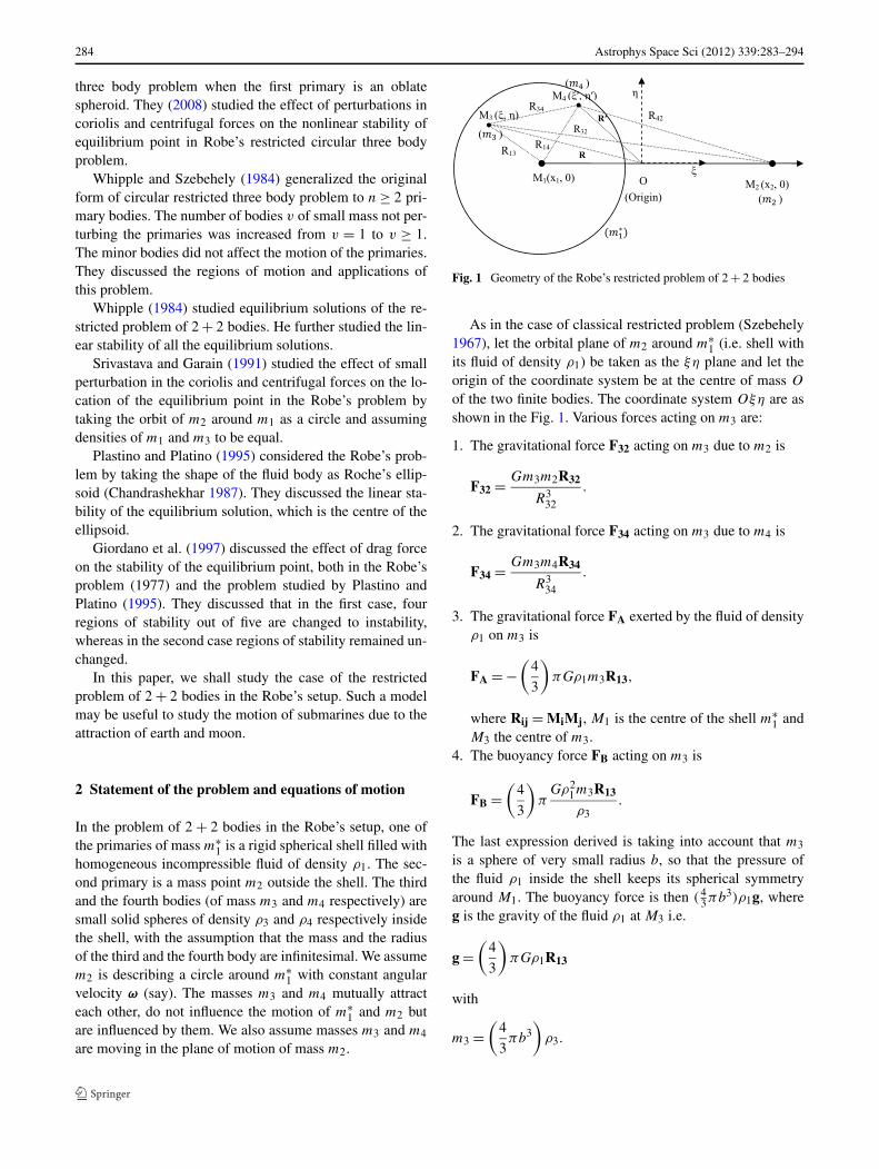
Fig. 1 Geometry of the Robe’s restricted problem of 2 + 2 bodies
As in the case of classical restricted problem (Szebehely1967), let the orbital plane of m2 around m∗
1 (i.e. shell withits fluid of density ρ1) be taken as the ξη plane and let theorigin of the coordinate system be at the centre of mass O
of the two finite bodies. The coordinate system Oξη are asshown in the Fig. 1. Various forces acting on m3 are:
1. The gravitational force F32 acting on m3 due to m2 is
F32 = Gm3m2R32
R332
.
2. The gravitational force F34 acting on m3 due to m4 is
F34 = Gm3m4R34
R334
.
3. The gravitational force FA exerted by the fluid of densityρ1 on m3 is
FA = −(
4
3
)πGρ1m3R13,
where Rij = MiMj, M1 is the centre of the shell m∗1 and
M3 the centre of m3.4. The buoyancy force FB acting on m3 is
FB =(
4
3
)π
Gρ21m3R13
ρ3.
The last expression derived is taking into account that m3
is a sphere of very small radius b, so that the pressure ofthe fluid ρ1 inside the shell keeps its spherical symmetryaround M1. The buoyancy force is then ( 4
3πb3)ρ1g, whereg is the gravity of the fluid ρ1 at M3 i.e.
g =(
4
3
)πGρ1R13
with
m3 =(
4
3πb3
)ρ3.
Astrophys Space Sci (2012) 339:283–294 285
The equation of motion of m3 in the inertial system is
R̈ = Gm2R32
R332
+ Gm4R34
R334
− 4
3πGρ1
(1 − ρ1
ρ3
)R13,
where R = OM3 and Rij = MiMj.Now, we determine the equation of motion of m3 in the
synodic system. Let us suppose that the coordinate sys-tem Oξη rotates with angular velocity ω. This is the sameas the angular velocity of m2 which is describing a circlearound m∗
1.In the rotating (synodic) system, the equation of motion
of m3 is
∂2r∂t2
+ 2ω × ∂r∂t
+ ω × (ω × r)
= Gm2R32
R332
+ Gm4R34
R334
− 4
3πGρ1
(1 − ρ1
ρ3
)R13 (1)
where r = OM3 and ω = ωk̂ = (constant).Let the coordinates of m3 and m4 be (ξ, η) and (ξ ′, η′)
respectively.The equations of motion of m3 in cartesian coordinates
are
ξ̈ − 2ωη̇ = − Gm2(ξ − x2)
[(ξ − x2)2 + η2] 32
− Gm4(ξ − ξ ′)[(ξ − ξ ′)2 + (η − η′)2] 3
2
− 4
3πGρ1
(1 − ρ1
ρ3
)(ξ − x1) + ω2ξ, (2)
η̈ + 2ωξ̇ = − Gm2η
[(ξ − x2)2 + η2] 32
− Gm4(η − η′)[(ξ − ξ ′)2 + (η − η′)2] 3
2
− 4
3πGρ1(1 − ρ1
ρ3)η + ω2η. (3)
Now, as m2 is moving around m∗1 in a circle of radius ‘a’
with angular velocity ω, we have
ω =√
G(m∗1 + m2)
a3.
We, now, fix the units such that m∗1 + m2 = 1, a = 1. We
choose t in such a way that G = 1.We further take
μ1 = m∗1
m∗1 + m2
, μ2 = m2
m∗1 + m2
so that μ1 + μ2 = 1.
Let μ2 = μ, (say), then μ1 = 1 − μ. Coordinates of m∗1
and m2 are (−μ,0), (1 − μ,0).In the new units ω = 1.The equations of motion of m3 in the dimensionless
cartesian coordinates are
ξ̈ − 2η̇ = Vξ , (4)
and
η̈ + 2ξ̇ = Vη, (5)
where
V = 1
2
(ξ2 + η2
)+ μ
R32+ μ4
R34− K
2
[(ξ + μ)2 + η2
](6)
and
μ4 = m4
m∗1 + m2
� 1, K = 4
3πρ1
(1 − ρ1
ρ3
). (7)
Similarly, in the rotating (synodic) system, the equations ofmotion of m4 in dimensionless cartesian coordinates are
ξ̈ ′ − 2η̇′ = V ′ξ ′ , (8)
η̈′ + 2ξ̇ ′ = V ′η′ , (9)
where
V ′ = 1
2
(ξ ′2 + η′2) + μ
R42+ μ3
R43− K ′
2
[(ξ ′ + μ
)2 + η′2]
(10)
and
μ3 = m3
m∗1 + m2
� 1, K ′ = 4
3πρ1
(1 − ρ1
ρ4
). (11)
3 Equilibrium solutions
The equilibrium solutions of m3 and m4 are given by
Vξ = 0 = Vη; V ′ξ ′ = 0 = V ′
η′
i.e.,
ξ − μ{ξ − (1 − μ)}
R332
− μ4(ξ − ξ ′)
R334
− K(ξ + μ) = 0, (12)
η − μη
R332
− μ4(η − η′)
R334
− Kη = 0 (13)
and
ξ ′ − μ{ξ ′ − (1 − μ)}
R342
− μ3(ξ ′ − ξ)
R343
− K ′(ξ ′ + μ) = 0,
(14)
286 Astrophys Space Sci (2012) 339:283–294
η′ − μη′
R342
− μ3(η′ − η)
R343
− K ′η′ = 0 (15)
Case I: Collinear Equilibrium Solutions
By inspection, we see that (13) and (15) are satisfied withη = η′ = 0.
It remains to determine ξ and ξ ′ such that the followingsimplified forms of (12) and (14) are satisfied, i.e.
ξ − μ{ξ − (1 − μ)}|ξ − (1 − μ)|3 − μ4
(ξ − ξ ′)|ξ − ξ ′|3 − K(ξ + μ) = 0, (16)
ξ ′ − μ{ξ ′ − (1 − μ)}|ξ ′ − (1 − μ)|3 − μ3
(ξ ′ − ξ)
|ξ ′ − ξ |3 − K ′(ξ ′ + μ) = 0.
(17)
When μ4 = 0, there exists only one equilibrium solution ofthe system, viz (−μ,0), (Hallan and Rana 2001a). Again,when μ3 = 0, (−μ,0) is the only equilibrium solution ofthe system. We now apply the perturbation theory when nei-ther μ3 nor μ4 is zero. We further define
(x,y) = 1
2(x2 + y2) + μ
[{x − (1 − μ)}2 + y2] 12
− K
2[(x + μ)2 + y2]
and
′(x, y) = 1
2(x2 + y2) + μ
[{x − (1 − μ)}2 + y2] 12
− K ′
2[(x + μ)2 + y2].
The solutions ξ and ξ ′ of (16) and (17) may be expressed aspower series in small parameters
εi = μi
(�μ3 + μ4)23
� 1, (i = 3,4) (18)
where
� = (3)xx
′(4)xx
.
The upper suffix (3) and (4) denote the evaluation of thederivatives at the equilibrium solution (−μ,0) for m3 andm4 respectively. We take
ξ = −μ +∞∑
j=1
a1j εj
4 , (19)
ξ ′ = −μ +∞∑
j=1
a2j εj
3 (Whipple and Szebehely 1984).
(20)
The equations (12), (13), (14), and (15) can be written as
x(ξ, η) − μ4(ξ − ξ ′)
R334
= 0, (21)
y(ξ, η) − μ4(η − η′)
R334
= 0, (22)
′x(ξ
′, η′) − μ3(ξ ′ − ξ)
R343
= 0, (23)
′y(ξ
′, η′) − μ3(η′ − η)
R343
= 0. (24)
To o(ε), where ε = max(ε3, ε4), by Taylor’s series, we have
x(ξ,0) = a11ε4(3)xx ,
′x(ξ
′,0) = a21ε3′(4)xx .
The equations (21) and (23) when η = η′ = 0 become
a11ε4(3)xx − μ4
(ξ − ξ ′)|ξ − ξ ′|3 = 0, (25)
a21ε3′(4)xx − μ3
(ξ ′ − ξ)
|ξ ′ − ξ |3 = 0. (26)
The equations (25) and (26) may be combined to yield
μ3a11ε4(3)xx + μ4a21ε3
′(4)xx = 0.
Since μ3ε4 = μ4ε3, we have
a11(3)xx + a21
′(4)xx = 0 or
a21 = −�a11.
(27)
To o(ε), using (19), (20), and (27) in (25), we have
|a11|3 = μ4
ε4(3)xx (ε4 + �ε3)2
.
Now, we have from (18)
ε4 + �ε3 = (μ4 + �μ3)13 .
Therefore,
a11 = ± 1
((3)xx )
13
.
Also,
a21 = −�a11 = ± 1
((3)xx )
13
(3)xx
′(4)xx
.
Astrophys Space Sci (2012) 339:283–294 287
Therefore, to o(ε), from (19), we have
ξ = −μ + a11ε4
= −μ ± μ4
[(μ4 + �μ3)2(3)xx ] 1
3
.
and from (20), we have
ξ ′ = −μ + a21ε3
= −μ ± 1
((3)xx )
13
(3)xx
′(4)xx
μ3
(μ4 + �μ3)23
.
Also,
(3)xx = 1 − K + 2μ,
′(4)xx = 1 − K ′ + 2μ.
Therefore,
ξ = −μ ± μ4
[(μ4 + �μ3)2(1 − K + 2μ)] 13
(28)
and
ξ ′ = −μ ± (1 − K + 2μ)23
(1 − K ′ + 2μ)
μ3
(μ4 + �μ3)23
. (29)
In the case when ρ3 = ρ4, we have
I. K = K ′II. (x,y) = ′(x, y)
III. (3)xx = 1 − K + 2μ = 1 − K ′ + 2μ =
′(4)xx
IV. � = 1
Therefore, ξ and ξ ′ become
ξ = −μ ± μ4
[(μ3 + μ4)2(1 − K + 2μ)] 13
, (30)
and
ξ ′ = −μ ± μ3
[(μ3 + μ4)2(1 − K + 2μ)] 13
. (31)
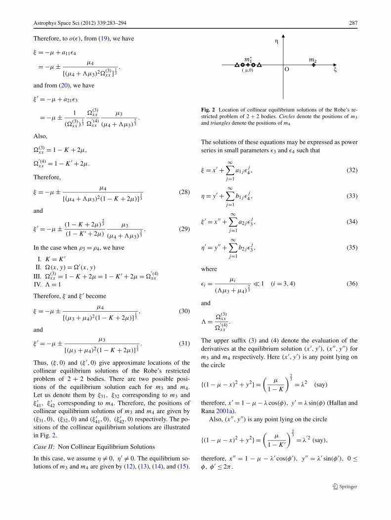
Thus, (ξ,0) and (ξ ′,0) give approximate locations of thecollinear equilibrium solutions of the Robe’s restrictedproblem of 2 + 2 bodies. There are two possible posi-tions of the equilibrium solution each for m3 and m4.Let us denote them by ξ31, ξ32 corresponding to m3 andξ ′
41, ξ ′42 corresponding to m4. Therefore, the positions of
collinear equilibrium solutions of m3 and m4 are given by(ξ31,0), (ξ32,0) and (ξ ′
41,0), (ξ ′42,0) respectively. The po-
sitions of the collinear equilibrium solutions are illustratedin Fig. 2.
Case II: Non Collinear Equilibrium Solutions
In this case, we assume η �= 0, η′ �= 0. The equilibrium so-lutions of m3 and m4 are given by (12), (13), (14), and (15).
Fig. 2 Location of collinear equilibrium solutions of the Robe’s re-stricted problem of 2 + 2 bodies. Circles denote the positions of m3and triangles denote the positions of m4
The solutions of these equations may be expressed as powerseries in small parameters ε3 and ε4 such that
ξ = x′ +∞∑
j=1
a1j εj
4 , (32)
η = y′ +∞∑
j=1
b1j εj
4 , (33)
ξ ′ = x′′ +∞∑
j=1
a2j εj
3 , (34)
η′ = y′′ +∞∑
j=1
b2j εj
3 , (35)
where
εi = μi
(�μ3 + μ4)23
� 1 (i = 3,4) (36)
and
� = (3)xx
′(4)xx
.
The upper suffix (3) and (4) denote the evaluation of thederivatives at the equilibrium solution (x′, y′), (x′′, y′′) form3 and m4 respectively. Here (x′, y′) is any point lying onthe circle
{(1 − μ − x)2 + y2} =(
μ
1 − K
) 23 = λ2 (say)
therefore, x′ = 1 − μ − λ cos(φ), y′ = λ sin(φ) (Hallan andRana 2001a).
Also, (x′′, y′′) is any point lying on the circle
{(1 − μ − x)2 + y2} =(
μ
1 − K ′
) 23 = λ
′2 (say),
therefore, x′′ = 1 − μ − λ′ cos(φ′), y′′ = λ′ sin(φ′), 0 ≤φ, φ′ ≤ 2π .
288 Astrophys Space Sci (2012) 339:283–294
The equations (12), (13), (14), and (15) can be written as(21), (22), (23), and (24).
To o(ε), where ε = max(ε3, ε4) and using the values ofξ, η, ξ ′, η′ from (32), (33), (34) and (35) and applyingTaylor’s series, the first term of (21) is
x(ξ, η) = a11ε4(3)xx + b11ε4
(3)xy . (37)
Similarly, we can determine y(ξ, η), ′x(ξ
′, η′), and′
y(ξ′, η′).
Since μ3,μ4, ε3, ε4 are very small, ignoring the higherorder terms and using (32), (33), (34) and (35), the secondterm of (21) is
μ4(ξ − ξ ′)
R334
= μ4(x′ − x′′)
[(x′ − x′′)2 + (y′ − y′′)2] 32
. (38)
Similarly
μ4(η − η′)
R334
= μ4(y′ − y′′)
[(x′ − x′′)2 + (y′ − y′′)2] 32
. (39)
Using (37), (38), (39), the equations (21), (22), (23), (24)become(a11
(3)xx + b11
(3)xy
)ε4 + μ4t1 = 0, (40)
(a11
(3)xy + b11
(3)yy
)ε4 + μ4t2 = 0, (41)
(a21
′(4)xx + b21
′(4)xy
)ε3 − μ3t1 = 0, (42)
(a21
′(4)xy + b21
′(4)yy
)ε3 − μ3t2 = 0, (43)
where
t1 = − (x′ − x′′)[(x′ − x′′)2 + (y′ − y′′)2] 3
2
, (44)
t2 = − (y′ − y′′)[(x′ − x′′)2 + (y′ − y′′)2] 3
2
. (45)
From (40) and (41), we have
a11 = μ4((3)xy t2 −
(3)yy t1)
ε4((3)xx
(3)yy − (
(3)xy )2)
,
b11 = μ4((3)xy t1 −
(3)xx t2)
ε4((3)xx
(3)yy − (
(3)xy )2)
.
From (42) and (43), we have
a21 = μ3(′(4)yy t1 −
′(4)xy t2)
ε3(′(4)xx
′(4)yy − (
′(4)xy )2)
,
b21 = μ3(′(4)xx t2 −
′(4)xy t1)
ε3(′(4)xx
′(4)yy − (
′(4)xy )2)
.
To o(ε), we get
ξ = x′ + a11ε4
= x′ + μ4((3)xy t2 −
(3)yy t1)
((3)xx
(3)yy − (
(3)xy )2)
= X1 (say), (46)
η = y′ + b11ε4
= y′ + μ4((3)xy t1 −
(3)xx t2)
((3)xx
(3)yy − (
(3)xy )2)
= Y1 (say). (47)
Also,
ξ ′ = x′′ + a21ε3
= x′′ + μ3(′(4)yy t1 −
′(4)xy t2)
(′(4)xx
′(4)yy − (
′(4)xy )2)
= X2 (say), (48)
η′ = y′′ + b21ε3
= y′′ + μ3(′(4)xx t2 −
′(4)xy t1)
(′(4)xx
′(4)yy − (
′(4)xy )2)
= Y2 (say), (49)
where
(3)xx = 3μ(Cos(φ))2
λ3,
(3)xy = −3μCos(φ)Sin(φ)
λ3,
(3)yy = 1 − μ
λ3+ 3μ(Sin(φ))2
λ3,
′(4)xx = 3μ(Cos(φ′))2
λ′3 ,
′(4)xy = −3μCos(φ′)Sin(φ′)
λ′3 ,
′(4)yy = 1 − μ
λ′3 + 3μ(Sin(φ′))2
λ′3
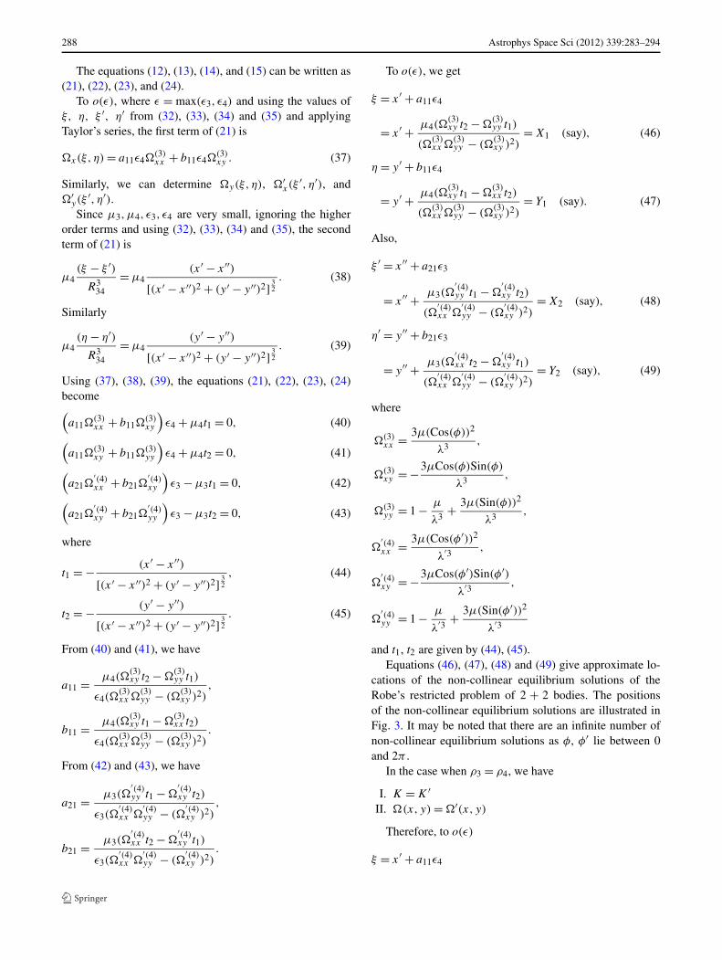
and t1, t2 are given by (44), (45).Equations (46), (47), (48) and (49) give approximate lo-
cations of the non-collinear equilibrium solutions of theRobe’s restricted problem of 2 + 2 bodies. The positionsof the non-collinear equilibrium solutions are illustrated inFig. 3. It may be noted that there are an infinite number ofnon-collinear equilibrium solutions as φ, φ′ lie between 0and 2π .
In the case when ρ3 = ρ4, we have
I. K = K ′II. (x,y) = ′(x, y)
Therefore, to o(ε)
ξ = x′ + a11ε4
Astrophys Space Sci (2012) 339:283–294 289
Fig. 3 Location of non collinear equilibrium solutions (ρ3 �= ρ4) ofthe Robe’s restricted problem of 2 + 2 bodies
= x′ + μ4((3)xy t2 −
(3)yy t1)
((3)xx
(3)yy − (
(3)xy )2)
. (50)
η = y′ + b11ε4
= y′ + μ4((3)xy t1 −
(3)xx t2)
((3)xx
(3)yy − (
(3)xy )2)
. (51)
Also,
ξ ′ = x′′ + a21ε3
= x′′ + μ3((4)yy t1 −
(4)xy t2)
((4)xx
(4)yy − (
(4)xy )2)
, (52)
η′ = y′′ + b21ε3
= y′′ + μ3((4)xx t2 −
(4)xy t1)
((4)xx
(4)yy − (
(4)xy )2)
. (53)
where
(3)xx = 3μ(Cos(φ))2
λ3,
(3)xy = −3μCos(φ)Sin(φ)
λ3,
(3)yy = 1 − μ
λ3+ 3μ(Sin(φ))2
λ3,
(4)xx = 3μ(Cos(φ′))2
λ3,
(4)xy = −3μCos(φ′)Sin(φ′)
λ3,
(4)yy = 1 − μ
λ3+ 3μ(Sin(φ′))2
λ3
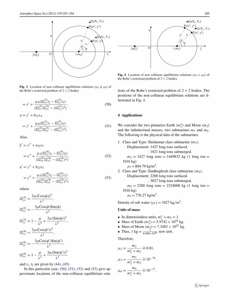
and t1, t2 are given by (44), (45).In this particular case, (50), (51), (52) and (53) give ap-
proximate locations of the non-collinear equilibrium solu-
Fig. 4 Location of non collinear equilibrium solutions (ρ3 = ρ4) ofthe Robe’s restricted problem of 2 + 2 bodies
tions of the Robe’s restricted problem of 2 + 2 bodies. Thepositions of the non-collinear equilibrium solutions are il-lustrated in Fig. 4.
4 Applications
We consider the two primaries Earth (m∗1) and Moon (m2)
and the infinitesimal masses, two submarines m3 and m4.The following is the physical data of the submarines.
1. Class and Type: Shishumar class submarine (m3).Displacement: 1427 long tons surfaced.
: 1821 long tons submerged.m3 = 1427 long tons = 1449832 kg (1 long ton =
1016 kg)ρ3 = 804.79 kg/m3.
2. Class and Type: Sindhughosh class submarine (m4).Displacement: 2288 long tons surfaced.
: 3027 long tons submerged.m4 = 2288 long tons = 2324608 kg (1 long ton =
1016 kg)ρ4 = 776.27 kg/m3.
Density of salt water (ρ1) = 1027 kg/m3.
Units of mass:
• In dimensionless units, m∗1 + m2 = 1.
• Mass of Earth (m∗1) = 5.9742 × 1024 kg.
• Mass of Moon (m2) = 7.3483 × 10²² kg.• Thus, 1 kg = 1
6.048×1024 new unit.
Therefore,
μ2 = m2
m∗1 + m2
∼= 0.01,
μ3 = m3
m∗1 + m2
∼= 10−18,
μ4 = m4
m∗1 + m2
∼= 10−17.
290 Astrophys Space Sci (2012) 339:283–294
Table 1 Collinear equilibrium solutions for m3 and m4 (ρ3 �= ρ4)
μ ξ31 ξ32 ξ ′41 ξ ′
42
0.0100 −0.00999992 −0.01000008 −0.009999990 −0.01000010
Units of distance:
Distance between Earth and Moon = 384400 km = 1 newunit.
Thus, 1 metre = 1384400000 new unit.
Hence,
ρ1 = 9317.7 new units,
ρ3 = 7301.65 new units,
ρ4 = 7040.45 new units,
K = 4
3πρ1
(1 − ρ1
ρ3
)= −10780.8,
K ′ = 4
3πρ1
(1 − ρ1
ρ4
)= −12629.4.
Table 1 gives the collinear equilibrium solutions for m3 andm4 using the above data. The numerical solutions are correctin all digits printed.
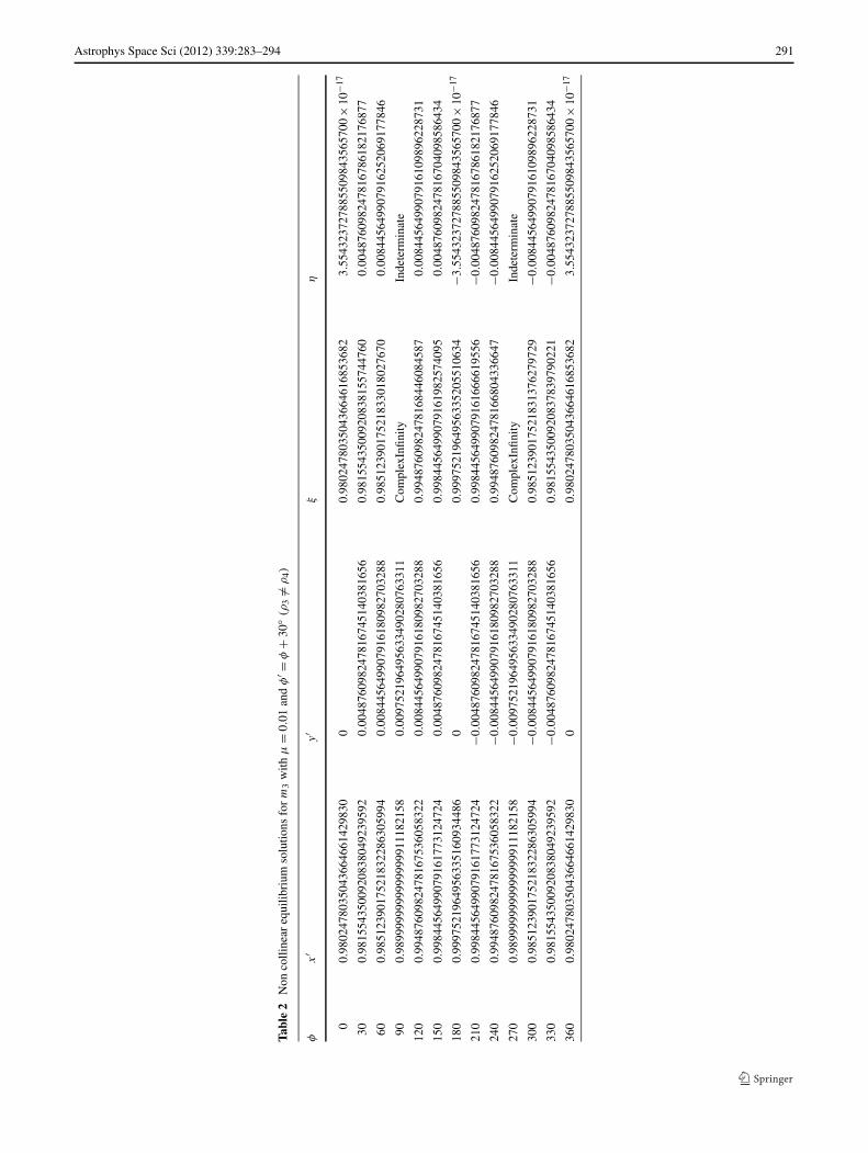
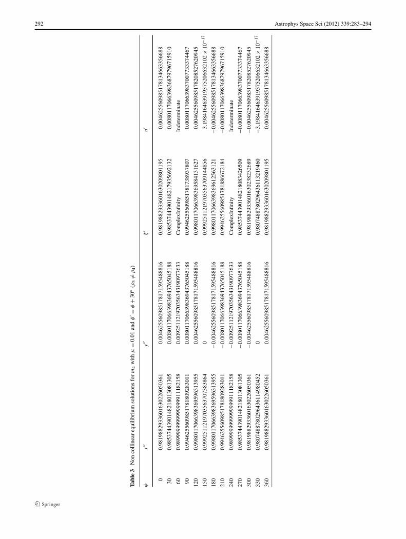
Tables 2 and 3 give non-collinear equilibrium solutionsfor m3 and m4 respectively with μ = 0.01 and φ′ = φ + 30◦(supposed) using the above data. The numerical solutionsare correct in all digits printed.
5 Stability of the equilibrium solutions
Let (X,Y ) be one of the equilibrium solution. Let it bedisplaced to (X + α,Y + β) where α,β � 1. Then ξ =X + α,η = Y + β .
The equations of motion (4) and (5) become
α̈ − 2β̇ = Vξ (X + α,Y + β) ,
β̈ + 2α̇ = Vη (X + α,Y + β) .
It maybe noted that for m3 it is V and for m4 it is V ′.Therefore, by Taylor’s series, we have,
α̈ − 2β̇ = αV(0)ξξ + βV
(0)ξη , (54)
β̈ + 2α̇ = αV(0)ξη + βV (0)
ηη (55)
where the upper suffix (0) denotes the evaluation of thederivatives at the equilibrium solution (X,Y ).
The characteristic equations of m3 and m4 are given by
λ41 − λ2
1
(V
(3)ξξ + V (3)
ηη − 4)
+(
V(3)ξξ V (3)
ηη −(V
(3)ξη
)2)
= 0. (56)
λ42 − λ2
2
(V
′(4)
ξ ′ξ ′ + V′(4)
η′η′ − 4)
+(
V′(4)
ξ ′ξ ′ V′(4)
η′η′ −(V
′(4)
ξ ′η′)2
)
= 0. (57)
Here the upper suffix (3) and (4) denote the evaluation ofthe derivatives at the equilibrium solutions.
The equation (56) has two roots in λ21. Let us denote them
by �11 and �12. Similarly the two roots of (57) in λ22 are
denoted by �21 and �22. The four roots of (56) in λ1 willbe ±√
�11,±√�12. Similarly the four roots of (57) in λ2
will be ±√�21,±√
�22.We have
λ21 = (V
(3)ξξ + V
(3)ηη − 4) ± √
d
2(58)
where
d =(V
(3)ξξ + V (3)
ηη − 4)2 − 4
(V
(3)ξξ V (3)
ηη −(V
(3)ξη
)2)
and
λ22 = (V
′(4)
ξ ′ξ ′ + V′(4)
η′η′ − 4) ± √d1
2(59)
where
d1 =(V
′(4)
ξ ′ξ ′ + V′(4)
η′η′ − 4)2 − 4
(V
′(4)
ξ ′ξ ′ V′(4)
η′η′ −(V
′(4)
ξ ′η′)2
).
In the case when ρ3 = ρ4 we have K = K ′. The eigenvaluescan be deduced from (58) and (59) by replacing K ′ by K .
If any of the roots of the characteristic equations (56) and(57) is positive and real, the corresponding equilibrium so-lution will be unstable.
Stability of collinear equilibrium solutions The positionsof collinear equilibrium solutions of m3 and m4 are givenby (ξ31,0), (ξ32,0) and (ξ ′
41,0), (ξ ′42,0) respectively. Four
cases arise.
Case I. The equilibrium solutions for m3 and m4 are at(ξ31,0), (ξ ′
41,0). Equation (56) has four roots in λ1. Letus denote them by ±λ11,±λ12. Similarly the roots of (57)in λ2 be denoted by ±λ21,±λ22.
Astrophys Space Sci (2012) 339:283–294 291
Tabl
e2
Non
colli
near
equi
libri
umso
lutio
nsfo
rm
3w
ithμ
=0.
01an
dφ
′ =φ
+30
◦(ρ
3�=
ρ4)
φx
′y
′ξ
η
00.
9802
4780
3504
3664
6614
2983
00
0.98
0247
8035
0436
6461
6853
682
3.55
4323
7278
8550
9843
5657
00×
10−1
7
300.
9815
5435
0092
0838
0492
3959
20.
0048
7609
8247
8167
4514
0381
656
0.98
1554
3500
9208
3815
5744
760
0.00
4876
0982
4781
6786
1821
7687
7
600.
9851
2390
1752
1832
2863
0599
40.
0084
4564
9907
9161
8098
2703
288
0.98
5123
9017
5218
3301
8027
670
0.00
8445
6499
0791
6252
0691
7784
6
900.
9899
9999
9999
9999
9111
8215
80.
0097
5219
6495
6334
9028
0763
311
Com
plex
Infin
ityIn
dete
rmin
ate
120
0.99
4876
0982
4781
6753
6058
322
0.00
8445
6499
0791
6180
9827
0328
80.
9948
7609
8247
8168
4460
8458
70.
0084
4564
9907
9161
0989
6228
731
150
0.99
8445
6499
0791
6177
3124
724
0.00
4876
0982
4781
6745
1403
8165
60.
9984
4564
9907
9161
9825
7409
50.
0048
7609
8247
8167
0409
8586
434
180
0.99
9752
1964
9563
3516
0934
486
00.
9997
5219
6495
6335
2055
1063
4−3
.554
3237
2788
5509
8435
6570
0×
10−1
7
210
0.99
8445
6499
0791
6177
3124
724
−0.0
0487
6098
2478
1674
5140
3816
560.
9984
4564
9907
9161
6666
1955
6−0
.004
8760
9824
7816
7861
8217
6877
240
0.99
4876
0982
4781
6753
6058
322
−0.0
0844
5649
9079
1618
0982
7032
880.
9948
7609
8247
8166
8043
3664
7−0
.008
4456
4990
7916
2520
6917
7846
270
0.98
9999
9999
9999
9991
1182
158
−0.0
0975
2196
4956
3349
0280
7633
11C
ompl
exIn
finity
Inde
term
inat
e
300
0.98
5123
9017
5218
3228
6305
994
−0.0
0844
5649
9079
1618
0982
7032
880.
9851
2390
1752
1831
3762
7972
9−0
.008
4456
4990
7916
1098
9622
8731
330
0.98
1554
3500
9208
3804
9239
592
−0.0
0487
6098
2478
1674
5140
3816
560.
9815
5435
0092
0837
8397
9022
1−0
.004
8760
9824
7816
7040
9858
6434
360
0.98
0247
8035
0436
6466
1429
830
00.
9802
4780
3504
3664
6168
5368
23.
5543
2372
7885
5098
4356
5700
×10
−17
292 Astrophys Space Sci (2012) 339:283–294
Tabl
e3
Non
colli
near
equi
libri
umso
lutio
nsfo
rm
4w
ithμ
=0.
01an
dφ
′ =φ
+30
◦(ρ
3�=
ρ4)
φx
′′y
′′ξ
′η
′
00.
9819
8829
3360
1630
2260
5036
10.
0046
2556
0985
1781
7159
5488
816
0.98
1988
2933
6016
3020
9801
195
0.00
4625
5609
8517
8134
6633
5668
8
300.
9853
7443
9014
8218
0130
8130
50.
0080
1170
6639
8369
4376
5045
188
0.98
5374
4390
1482
1793
5692
132
0.00
8011
7066
3983
6879
7967
1591
0
600.
9899
9999
9999
9999
9111
8215
80.
0092
5112
1970
3563
4319
0977
633
Com
plex
Infin
ityIn
dete
rmin
ate
900.
9946
2556
0985
1781
8092
8301
10.
0080
1170
6639
8369
4376
5045
188
0.99
4625
5609
8517
8173
8937
807
0.00
8011
7066
3983
7007
7333
7446
7
120
0.99
8011
7066
3983
6959
6313
955
0.00
4625
5609
8517
8171
5954
8881
60.
9980
1170
6639
8369
5841
3162
70.
0046
2556
0985
1782
0852
7620
945
150
0.99
9251
1219
7035
6370
7383
864
00.
9992
5112
1970
3563
7091
4485
63.
1984
1646
3919
3752
0663
2102
×10
−17
180
0.99
8011
7066
3983
6959
6313
955
−0.0
0462
5560
9851
7817
1595
4888
160.
9980
1170
6639
8369
6125
6312
1−0
.004
6255
6098
5178
1346
6335
6688
210
0.99
4625
5609
8517
8180
9283
011
−0.0
0801
1706
6398
3694
3765
0451
880.
9946
2556
0985
1781
8866
7218
4−0
.008
0117
0663
9836
8797
9671
5910
240
0.98
9999
9999
9999
9991
1182
158
−0.0
0925
1121
9703
5634
3190
9776
33C
ompl
exIn
finity
Inde
term
inat
e
270
0.98
5374
4390
1482
1801
3081
305
−0.0
0801
1706
6398
3694
3765
0451
880.
9853
7443
9014
8218
0834
2650
9−0
.008
0117
0663
9837
0077
3337
4467
300
0.98
1988
2933
6016
3022
6050
361
−0.0
0462
5560
9851
7817
1595
4888
160.
9819
8829
3360
1630
2382
3268
9−0
.004
6255
6098
5178
2085
2762
0945
330
0.98
0748
8780
2964
3611
4980
452
00.
9807
4887
8029
6436
1132
1946
0−3
.198
4164
6391
9375
2066
3210
2×
10−1
7
360
0.98
1988
2933
6016
3022
6050
361
0.00
4625
5609
8517
8171
5954
8881
60.
9819
8829
3360
1630
2098
0119
50.
0046
2556
0985
1781
3466
3356
688
Astrophys Space Sci (2012) 339:283–294 293
Table 4 Stability of collinear equilibrium solutions for m3 (ρ3 �= ρ4)
μ ±λ11 ±λ12 ±λ13 ±λ14
0.01 ±209.7086117726478780465229 ±76.27799490163028638359341i ±175.0584407696850689792168 ±29.12181592076459177443333
μ ±λ15 ±λ16 ±λ17 ±λ18
0.01 ±175.0584407696534164331535 ±29.12181592085973434748463 ±209.7086117726214566887602 ±76.27799490159396574617318i
Table 5 Stability of non-collinear equilibrium solutions for m3 with μ = 0.01 and φ′ = φ + 30◦(ρ3 �= ρ4)
φ (degree) ±√�11 ±√
�12
0 ±179.8374382023723853403734 ±0.00001608049389644347143414969
30 ±179.8374382023725398901880 ±0.00001513658262928219503520821
60 ±Indeterminate ±Indeterminate
90 ±Indeterminate ±Indeterminate
120 ±179.8374382023729966183127 ±0.00001229815020923473960583077
150 ±179.8374382023733063735463 ±9.574681259814230138424997 × 10⁻⁶
180 ±179.8374382023723853403734 ±0.00001608049389644347143414969
210 ±179.8374382023725398901880 ±0.00001513658262928219503520821
240 ±Indeterminate ±Indeterminate
270 ±Indeterminate ±Indeterminate
300 ±179.8374382023729966183127 ±0.00001229815020923473960583077
330 ±179.8374382023733063735463 ±9.574681259814230138424997 × 10⁻⁶
360 ±179.8374382023723853403734 ±0.00001608049389644347143414969
Case II. The equilibrium solutions for m3 and m4 are at(ξ31,0), (ξ ′
42,0).
Equation (56) has four roots in λ1. Let us denote them by±λ13,±λ14. Similarly the roots of (57) in λ2 be denoted by±λ23,±λ24.
Case III. The equilibrium solutions for m3 and m4 are at(ξ32,0), (ξ ′
41,0). Equation (56) has four roots in λ1. Let usdenote them by ±λ15,±λ16. Similarly the roots of (57) inλ2 be denoted by ±λ25,±λ26.
Case IV. The equilibrium solutions for m3 and m4 are at(ξ32,0), (ξ ′
42,0). Equation (56) has four roots in λ1. Let usdenote them by ±λ17,±λ18. Similarly the roots of (57) inλ2 be denoted by ±λ27,±λ28.
If any of the four roots described above in each case arepositive and real, the equilibrium solution is unstable other-wise stable.
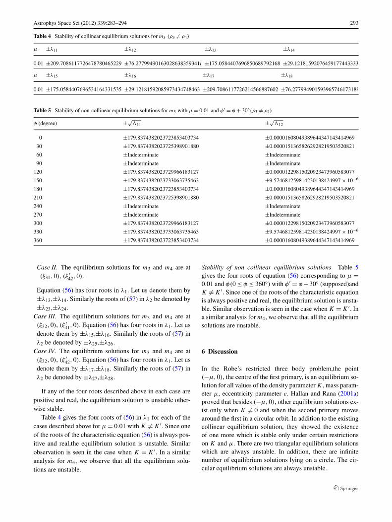
Table 4 gives the four roots of (56) in λ1 for each of thecases described above for μ = 0.01 with K �= K ′. Since oneof the roots of the characteristic equation (56) is always pos-itive and real,the equilibrium solution is unstable. Similarobservation is seen in the case when K = K ′. In a similaranalysis for m4, we observe that all the equilibrium solu-tions are unstable.
Stability of non collinear equilibrium solutions Table 5gives the four roots of equation (56) corresponding to μ =0.01 and φ(0 ≤ φ ≤ 360◦) with φ′ = φ +30◦ (supposed)andK �= K ′. Since one of the roots of the characteristic equationis always positive and real, the equilibrium solution is unsta-ble. Similar observation is seen in the case when K = K ′. Ina similar analysis for m4, we observe that all the equilibriumsolutions are unstable.
6 Discussion
In the Robe’s restricted three body problem,the point(−μ,0), the centre of the first primary, is an equilibrium so-lution for all values of the density parameter K , mass param-eter μ, eccentricity parameter e. Hallan and Rana (2001a)proved that besides (−μ,0), other equilibrium solutions ex-ist only when K �= 0 and when the second primary movesaround the first in a circular orbit. In addition to the existingcollinear equilibrium solution, they showed the existenceof one more which is stable only under certain restrictionson K and μ. There are two triangular equilibrium solutionswhich are always unstable. In addition, there are infinitenumber of equilibrium solutions lying on a circle. The cir-cular equilibrium solutions are always unstable.
294 Astrophys Space Sci (2012) 339:283–294
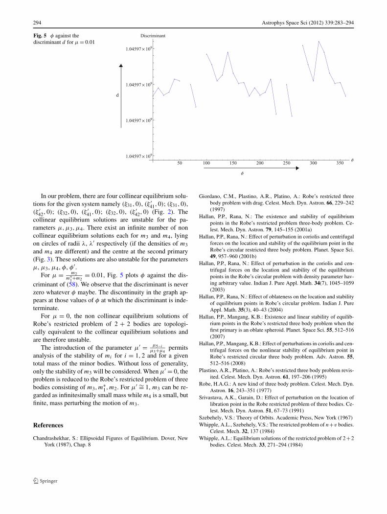
Fig. 5 φ against thediscriminant d for μ = 0.01
In our problem, there are four collinear equilibrium solu-tions for the given system namely (ξ31,0), (ξ ′
41,0); (ξ31,0),(ξ ′
42,0); (ξ32,0), (ξ ′41,0); (ξ32,0), (ξ ′
42,0) (Fig. 2). Thecollinear equilibrium solutions are unstable for the pa-rameters μ,μ3,μ4. There exist an infinite number of noncollinear equilibrium solutions each for m3 and m4, lyingon circles of radii λ, λ′ respectively (if the densities of m3
and m4 are different) and the centre at the second primary(Fig. 3). These solutions are also unstable for the parametersμ, μ3, μ4, φ, φ′.
For μ = m2m∗
1+m2= 0.01, Fig. 5 plots φ against the dis-
criminant of (58). We observe that the discriminant is neverzero whatever φ maybe. The discontinuity in the graph ap-pears at those values of φ at which the discriminant is inde-terminate.
For μ = 0, the non collinear equilibrium solutions ofRobe’s restricted problem of 2 + 2 bodies are topologi-cally equivalent to the collinear equilibrium solutions andare therefore unstable.
The introduction of the parameter μ′ = μ5−i
μ3+μ4permits
analysis of the stability of mi for i = 1,2 and for a giventotal mass of the minor bodies. Without loss of generality,only the stability of m3 will be considered. When μ′ = 0, theproblem is reduced to the Robe’s restricted problem of threebodies consisting of m3,m
∗1,m2. For μ′ ∼= 1, m3 can be re-
garded as infinitesimally small mass while m4 is a small, butfinite, mass perturbing the motion of m3.
References
Chandrashekhar, S.: Ellipsoidal Figures of Equilibrium. Dover, NewYork (1987), Chap. 8
Giordano, C.M., Plastino, A.R., Platino, A.: Robe’s restricted threebody problem with drag. Celest. Mech. Dyn. Astron. 66, 229–242(1997)
Hallan, P.P., Rana, N.: The existence and stability of equilibriumpoints in the Robe’s restricted problem three-body problem. Ce-lest. Mech. Dyn. Astron. 79, 145–155 (2001a)
Hallan, P.P., Rana, N.: Effect of perturbation in coriolis and centrifugalforces on the location and stability of the equilibrium point in theRobe’s circular restricted three body problem. Planet. Space Sci.49, 957–960 (2001b)
Hallan, P.P., Rana, N.: Effect of perturbation in the coriolis and cen-trifugal forces on the location and stability of the equilibriumpoints in the Robe’s circular problem with density parameter hav-ing arbitrary value. Indian J. Pure Appl. Math. 34(7), 1045–1059(2003)
Hallan, P.P., Rana, N.: Effect of oblateness on the location and stabilityof equilibrium points in Robe’s circular problem. Indian J. PureAppl. Math. 35(3), 40–43 (2004)
Hallan, P.P., Mangang, K.B.: Existence and linear stability of equilib-rium points in the Robe’s restricted three body problem when thefirst primary is an oblate spheroid. Planet. Space Sci. 55, 512–516(2007)
Hallan, P.P., Mangang, K.B.: Effect of perturbations in coriolis and cen-trifugal forces on the nonlinear stability of equilibrium point inRobe’s restricted circular three body problem. Adv. Astron. 55,512–516 (2008)
Plastino, A.R., Platino, A.: Robe’s restricted three body problem revis-ited. Celest. Mech. Dyn. Astron. 61, 197–206 (1995)
Robe, H.A.G.: A new kind of three body problem. Celest. Mech. Dyn.Astron. 16, 243–351 (1977)
Srivastava, A.K., Garain, D.: Effect of perturbation on the location oflibration point in the Robe restricted problem of three bodies. Ce-lest. Mech. Dyn. Astron. 51, 67–73 (1991)
Szebehely, V.S.: Theory of Orbits. Academic Press, New York (1967)Whipple, A.L., Szebehely, V.S.: The restricted problem of n+v bodies.
Celest. Mech. 32, 137 (1984)Whipple, A.L.: Equilibrium solutions of the restricted problem of 2+2
bodies. Celest. Mech. 33, 271–294 (1984)


![Solving the Latin square completion problem by memetic ...hao/papers/JinHaoIEEE2019.pdfparticular graph coloring problem (i.e., precoloring extension [5], then list coloring [12],](https://img.pdfslide.net/doc/110x75/5f1bd3fdfab8ed17bc38532a/solving-the-latin-square-completion-problem-by-memetic-haopapersjinhaoieee2019pdf.jpg)


![Blasius Problem and Falkner-Skan model: Töpfer’s Algorithm ... · Blasius Problem and Falkner-Skan model: Töpfer’s Algorithm and its Extension Riccardo Fazio ... man [12] reformulate](https://img.pdfslide.net/doc/110x75/5d4140d188c9938c3f8dce76/blasius-problem-and-falkner-skan-model-toepfers-algorithm-blasius-problem.jpg)