HAL Id: lirmm-01310817https://hal-lirmm.ccsd.cnrs.fr/lirmm-01310817

Submitted on 3 May 2016

HAL is a multi-disciplinary open accessarchive for the deposit and dissemination of sci-entific research documents, whether they are pub-lished or not. The documents may come fromteaching and research institutions in France orabroad, or from public or private research centers.

L’archive ouverte pluridisciplinaire HAL, estdestinée au dépôt et à la diffusion de documentsscientifiques de niveau recherche, publiés ou non,émanant des établissements d’enseignement et derecherche français ou étrangers, des laboratoirespublics ou privés.

Robotic Test Bench for CubeSat Ground Testing:Concept and Satellite Dynamic Parameter Identification

Irina Gavrilovich, Sébastien Krut, Marc Gouttefarde, François Pierrot,Laurent Dusseau

To cite this version:Irina Gavrilovich, Sébastien Krut, Marc Gouttefarde, François Pierrot, Laurent Dusseau. RoboticTest Bench for CubeSat Ground Testing: Concept and Satellite Dynamic Parameter Identifica-tion. IROS: Intelligent RObots and Systems, Sep 2015, Hamburg, Germany. pp.5447-5453,�10.1109/IROS.2015.7354148�. �lirmm-01310817�

Abstract— This paper introduces a novel concept of an air bearing test bench for CubeSat ground testing together with the corresponding dynamic parameter identification method. Contrary to existing air bearing test benches, the proposed concept allows three degree-of-freedom unlimited rotations and minimizes the influence of the test bench on the tested CubeSat. These advantages are made possible by the use of a robotic wrist which rotates air bearings in order to make them follow the CubeSat motion. Another keystone of the test bench is an accurate balancing of the tested CubeSat. Indeed, disturbing factors acting on the satellite shall be minimized, the most significant one being the gravity torque. An efficient balancing requires the CubeSat center of mass position to be accurately known. Usual techniques of dynamic parameter identification cannot be directly applied because of the frictionless suspension of the CubeSat in the test bench and, accordingly, due to the lack of external actuation. In this paper, a new identification method is proposed. This method does not require any external actuation and is based on the sampling of free oscillating motions of the CubeSat mounted on the test bench.

I. INTRODUCTION One of the widespread and demanded branches of space

technologies is CubeSat-class satellites. CubeSats are miniaturized satellites with standardized sizes of one-unit (1U, 10x10x10 mm), or a multiple of one unit (e.g. 3U). The development of such satellites is common in schools and universities due to the relatively short development time, the wide range of components available off-the-shelf, and compatibility with standardized launch ejectors. In addition to educational purposes, nowadays, CubeSats are employed in full scale scientific and technological missions, and every year the number of professional CubeSat programs increases [1]. This tendency leads to the necessity of complete CubeSat ground testing. One of the main issues of the pre-launch examination is the inspection of the Attitude Determination and Control System (ADCS) once it is assembled and integrated in the satellite. ADCS testing, unlike tests of other subsystems, requires the satellite to move. Each constraint impairing the satellite free rotation yields cases where the ADCS cannot be checked and might thus cause problems during its on-orbit operation. Results obtained for the available range of angles are often extrapolated to other

* Research supported by Van Allen Foundation and FEDER. 1 I. Garilovich, S. Krut, M. Gouttefarde, and F. Pierrot are with

the Montpellier Laboratory of Informatics, Robotics and Microelectronics (LIRMM), University of Montpellier and CNRS, 34090 Montpellier, France (e-mails: irina.gavrilovich/sebastien.krut/ marc.gouttefarde/francois.pierrot@lirmm.fr).

2 L. Dusseau is with the Centre Spatial Universitaire (CSU), University of Montpellier, 34090 Montpellier, France (e-mails: laurent.dusseau@ies.univ-montp2.fr)

attitudes in order to confirm ADCS operability, which decreases the probability of faultless operation.

The development of an ADCS test bench is a challenging task, but some examples can be found in the literature. Most of the developed test benches are designed for satellites with a mass greater than 50 kg [2]-[9]. They cannot be used for CubeSat ADCS tests, because inertia parameters of the test bench are critical for a reliable checkout and shall be comparable with those of the tested satellite. Some test benches have been designed specifically for CubeSats [10]-[12], but their maximum rotation angle is approximately 90° or less.

In this paper, a novel approach to the design of 1..3U CubeSat test benches is proposed. The corresponding design eliminates the limitations on the satellite attitude (orientation) during the testing since it allows full three degree-of-freedom (DoF) satellite rotations. The test bench consists of two frames, which have spherical mating surfaces conventionally called Spheres, and of a 4 DoF redundant robotic wrist. Moreover, four air bearings are employed to allow frictionless motion of the satellite mounted on the test bench.

Reliable and trustworthy results of ADCS testing can be obtained only if the effects of all disturbing torques caused by gravity, aerodynamic drag, and friction, are minimized. The total disturbing torque shall be one order of magnitude smaller than the total expected external torque on the orbit [8]. While other sources of disturbances can be reduced up to negligible values by optimizing environmental conditions at the test facility, the torque due to gravity always influences the satellite when there is an offset between the satellite center of mass (CM) and the test bench center of rotation (CR). A balancing procedure, aiming at eliminating this offset, requires an accurate identification of the satellite CM position together with its inertial parameters. In the sequel, the inertial parameters and the CM position are referred to as the dynamic parameters.

The identification of dynamic parameters is a well-known technique in robotics and related fields. Several approaches have been proposed in the literature to solve the dynamic parameter identification problem [2], [13]-[18]. Some common features of these approaches can be found in [15], [18], namely:

• The use of inverse dynamic or energy model to form the identification equations;

• The use of an optimal exciting trajectory for efficient model sampling;

• The use of an over-determinate linear system of equations resulting from the model sampling;

• Solving the linear system by the Least Squares method to estimate the parameters.

In all the aforementioned approaches, the identification is done for systems subjected to external actuation (usually,

Robotic Test Bench for CubeSat Ground Testing: Concept and Satellite Dynamic Parameter Identification*

Irina Gavrilovich1, Sébastien Krut1, Marc Gouttefarde1, François Pierrot1, and Laurent Dusseau2

2015 IEEE/RSJ International Conference on Intelligent Robots and Systems (IROS)Congress Center HamburgSept 28 - Oct 2, 2015. Hamburg, Germany

978-1-4799-9994-1/15/$31.00 ©2015 IEEE 5447

Figure 2. The test bench.

Figure 1. An air-levitated sphere and a spherical structure of the same

diameter formed by several air bearings.

joint forces/torques). For example in [2], where the identification and balancing of an 800 kg satellite is done, the test bench uses reaction wheels for actuation. The identification equations can be written in the following general form

( ) =y Γ W x (1)

where Γ is an external torque, W is an observation matrix, and x is the vector of the dynamic parameters to be identified. In the case of a passive system (with no actuation), the right-hand side of (1) is always equal to zero. The latter case is the one dealt with in this paper where the identification problem concerns the payload of the test bench which is passive, i.e., it is not subjected to external influences apart from the torque due to gravity. A method of dynamic parameter identification suitable to this passive case and based on the sampling of free oscillating rotations is presented in this paper.

In summary, the first contribution of this paper is a novel design of an air bearing test bench for CubeSat ADCS testing, which includes a 4-DoF redundant robotic wrist. The second contribution is a dynamic parameter identification technique for a passive system. This technique is based on the observation of its oscillating rotational motions.

The paper is organized as follows: Section 2 introduces the details of the test bench design, Sections 3 and 4 are devoted to the identification method. Section 5 presents simulation results while section 6 concludes the paper.

II. THE TEST BENCH The most popular and advanced technique to obtain

frictionless 3-DoF rotational motions of a satellite on a test bench is the use of air bearings. Different types of air bearing test benches are discussed in [19], but all of these designs have limitations on the available pitch and roll rotations of the mounted payload, the maximum rotation amplitudes being around ±45°. These limitations could be eliminated if the payload is placed at the center of a hollow sphere gliding on an air bearing puck. Such an approach was tried for satellite disassembled hardware, the system provided rotations of ±180° but the reported tests included single-axis rotations only [20]. In [9], an air-levitated sphere with a 1U CubeSat placed inside is described, but it was not realized because of technological issues. A hollow sphere able to hold 3U CubeSats would be bulky and heavy, which are undesirable characteristics for a CubeSat test bench. Another disadvantage is technological complexity: The hollow sphere shall be built in several sections to be able to place a payload inside the sphere, while the surface shall be accurately machined to provide the roughness required by the air bearings. The design proposed in this paper has the advantage of the air-levitated sphere (satellite unconstrained rotations) without its aforementioned weaknesses.

A. Concept The key advantage of the hollow sphere is the continuous

surface that allows friction-free contact with the bearing puck at every possible angular position. The idea proposed here is that the same property can be achieved by means of

several small air bearings rotating around a common CR placed at the spherical surface center (Fig. 1). The inner part of the structure, which consists of small hemispheres (spherical segments) as shown in the right part of Fig. 1, becomes much smaller and lighter than the air-levitated spheres suggested before. It is relevant to minimize the size and mass of this part of the test bench because of its unwanted moment of inertia. The frame on which the bearing pucks are attached, called the “External Sphere”, needs to follow the motion of the fictitious “Inner Sphere” wherein the satellite is mounted. The External Sphere is independent from the CubeSat mounted on the test bench and, therefore, has no influence on results of the tests.

B. Design overview The proposed CubeSat test bench mainly consists of

three parts: (i) the Inner Sphere composed of the sliding hemispheres attached to the CubeSat; (ii) the External Sphere built of the air bearing pucks; and (iii) a 4 DoF redundant robotic wrist, able to rotate the External Sphere around the CR (Figure 2). The External Sphere shall be rotated around the CR in order to follow the motion of the Inner Sphere so that each hemisphere remains aligned with its air bearing puck. The CR is thus common to both the

5448

Figure 3. The frames involved in the identification process.

Inner and External Spheres and is coincident with the common intersection point of the four robotic wrist revolute joint axes. While the whole system needs only 3 rotational DoF, the additional DoF of the wrist aims at eliminating kinematic singularities which would limit the possible rotations.

The CubeSat is fixed to the Inner Sphere by means of an adjusting mechanism, which allows limited modifications of the satellite position with respect to the CR. This feature is needed for sampling the payload motion with different initial offsets between the CR and the CM and for the final balancing of the CubeSat. The maximum displacements of the satellite inside the Inner Sphere are ±20 mm along the X and Y directions and ±35 mm in the Z direction. These values have been chosen according to CubeSat Design Specification [21] that defines allowable CM locations for 1...3U CubeSats.

The motion of the satellite is a key point of ADCS tests and shall not be predicted but only observed. Moreover, the positioning of the External Sphere has to be corrected rapidly based on the current position of the satellite. For these purposes, a tracking system is required. Two possible means to observe the Inner Sphere motion are: 3D motion capture cameras or distance sensors. The sensors measure a relative position of the hemispheres and pucks. In order to obtain an absolute estimation of the Inner Sphere attitude, the encoders of the robotic wrist joints are then required.

III. THE DYNAMICS OF THE TEST BENCH PAYLOAD

The payload of the test bench is the CubeSat together with the Inner Sphere and the adjusting mechanism, which are rigidly connected and move as one body. Before dynamic parameter identification, the dynamics of the payload shall be described. In the sequel, “body” refers to the payload.

A. Frames The inertial fixed frame IR is defined by the basis IB ,

denoted ( ), ,I I Ix y z , and its origin centered at the point CR . Vector Iz is aligned with the local vertical (Fig. 3). Let the basis bfB , denoted ( ), ,x y z , be attached to the body, and let the body-fixed reference frame bfR consist of bfB centered at a given point O of the body. The choice of O will be discussed in Section 4.

The frame BFR shown in Fig. 3 has the same orientation as bfB but its origin is CR . As shown in the sequel, the

frame BFR is introduced to simplify the writing of the equations of motion, suitable for identification. The position of the point CM in BFR is defined by the column vector ρ . As shown in Fig. 3, it can be written as the sum of the vectors

Oρ and r expressed in bfB

= + Oρ r ρ (2)

It should be noted that the vector r is related to the position of the body in BFR and the vector Oρ is constant for the given body (Fig. 3).

B. Kinematics The orientation of BFR with respect to IR is given by

the rotation matrix IBFA . In IB , the angular velocity vector

of the body Iω can be found as follows

[ ] T× =I I I

BF BFω A A& (3)

where [ ] ×Iω is the skew-symmetric matrix associated to the

vector Iω . The following operation can be used to express the angular velocity vector ω in bfB

= BF IIω A ω (4)

In the sequel, all vectors without a left superscript are expressed in bfB .

C. Dynamics The Euler’s equations of motion traditionally describes

the rotational dynamics of a body with respect to a coordinate frame whose origin is the body’s CM. The test bench payload is subjected to the action of a gravity torque (when the points CR and CM are not perfectly coincident) and to the reaction forces at the air bearings. The reaction forces are pointing towards CR . They can be represented by a resulting force passing through CR . The magnitude and direction of this force are unknown.

However, the equations of motion does not include this unknown resulting force if the Euler’s equations of motion are expressed in BFR

+ × =CR CR CRI ω ω I ω T& (5)

where CRI is the inertia matrix of the body at CR , CRT is the torque induced at CR by the weight mg of the body

[ ] [ ]m m m× ×= × = − = −CR BF IIT ρ g g ρ A g ρ (6)

Substituting (6) into (5) results in

[ ]m ×+ × + =CR CR BF III ω ω I ω A g ρ 0& (7)

Equation (7) describes the dynamics of the test bench payload in bfB . As detailed in Section 4, this equation can

5449

be used to obtain the identification equations in the following form

Φx = b (8)

where vector x contains the body dynamic parameters to be identified.

IV. IDENTIFICATION OF THE DYNAMIC PARAMETERS The goal of the identification process is to find the

dynamic parameters of the body. The dynamic model (7) in the current formulation is a function of these parameters taken with respect to CR ( CRI and ρ ) so that the vector bin (8) is always equal to zero. Moreover, CRI and ρ are related to the position of the body in BFR , hence the result of the identification depends on the initial position of the body with respect to CR . Such an objectionable situation can be avoided if the dynamic parameters are taken at a point attached to the body. The points CM and O (Fig. 3) are two candidate points. Choosing CM yields nonlinearities in the dynamic parameters. On the contrary, choosing O leads to a linear system. CRI and ρ shall thus be expressed with respect to O and substituted into (7).

A. The Inertia Matrix The inertia matrix CMI taken at CM and expressed in

bfB is:

CM CM CMxx xy xzCM CM CMxy yy yzCM CM CMxz yz zz

I I II I II I I

=

CMI (9)

Then, CRI can be found by applying the Huygens-Steiner theorem:

( )T Tm= + −CR CMI I ρ ρ 1 ρ ρ (10)

where 1 is the 3 3× identity matrix. Substituting (2) into (10) gives

( ) ( ) ( )( )( )( )( )( ) 2

T T

T T T

mm

= + + + − + += + + − +

CR CM O O O O

O O O O

I I ρ r ρ r 1 ρ r ρ rI C r ρ r1 ρ r rρ

(11)

where ( )T Tm= + −O CM O O O OI I ρ ρ 1 ρ ρ (12)

is the inertia matrix of the body taken at O and expressed in bfB and

( ) ( )T Tm= −C r r r1 r r (13)

is a value depending only on the position of the body in BFR and on the body’s mass m. The decomposition of the

inertia matrix presented in (11) is convenient for further simplification and transformation of (7).

B. The Identification Equations Taking into account the relations obtained in the previous

section, (7) can be rewritten as a linear equation in the

dynamic parameters. The product of the inertia matrix and the angular velocity becomes

( )( ) ,m= + +CR O OI ω I ω C r ω B ω r ρ (14)

where matrix ( ),B ω r is defined as

( )2 2 3 3 2 1 1 2 3 1 1 3

1 2 2 1 1 1 3 3 3 2 2 3

1 3 3 1 2 3 3 2 1 1 2 2

ω ω 2 ω ω 2 ω ω, 2 ω ω ω ω 2 ω ω

2 ω ω 2 ω ω ω ω

r r r r r rr r r r r rr r r r r r

− − − − = − − − −

− − − − B ω r (15)

Equation (14) can be modified to highlight the fact that it is linear in the unknown values OI and Oρ . The first term on the right-hand side can be written

( )O OI ω = Ω ω j (16)

where Oj is a 6 1× vector composed of the elements of the inertia matrix OI and ( )Ω ω is a 3 6× matrix composed of the elements of the vector ω

[ ]TO O O O O Oxx yy zz xy xz yzI I I I I I=Oj (17)

( )1 2 3

2 1 3

3 1 2

ω 0 0 ω ω 00 ω 0 ω 0 ω0 0 ω ω ω 0

=

Ω ω (18)

Accordingly, the expression of CRI ω& can be written as

( ) ( ) ( ),m= + +CR O OI ω Ω ω j B ω r ρ C r ω& & & & (19)

Collecting all dynamic parameters on the left-hand side, (7) is finally written in matrix form as

( ) [ ] ( ) [ ] [ ]( )[ ] [ ]

( ()

))

,(

)(

,mm

× × ×

× ×

+ + + = − − −

O

OjΩ ω ω Ω ω B ω B g ρ

g r ω C r ωω ωω

rC

rr&&&

(20)

C. The Least Squares Solution In this work, the identification of the components of the

inertia matrix and of the position of CM is based on the knowledge of the angular position of the body-fixed frame with respect to IR . A Least Squares (LS) solution requires data obtained from p experiments each having a duration of

iN sec or in time steps. iN and p as well as the initial conditions of the experiments should be optimized in order to obtain the best results. During the experiments, the body is moving freely under the influence of the gravity torque created by the body weight when CM is not coincident with CR . In each experiment, the initial conditions, i.e. the offset between CR and O , described by the vector ir , the initial orientation of the body in IR and its initial angular velocity could be different.

For the thj measurement of the thi experiment, (20) is

( ) [ ] ( ) [ ] [ ]( )[ ] [ ]

, )( ((

, ))()

ij iij ij ijij ij

ij i ij i

i i

ij

j

i ij

mm

× × ×

× ×

+ + + =− − −

O

OjΩω ω Ωω B ω B g ρ

g r ω C ω Cω r ω r

r r ω&&& (21)

5450

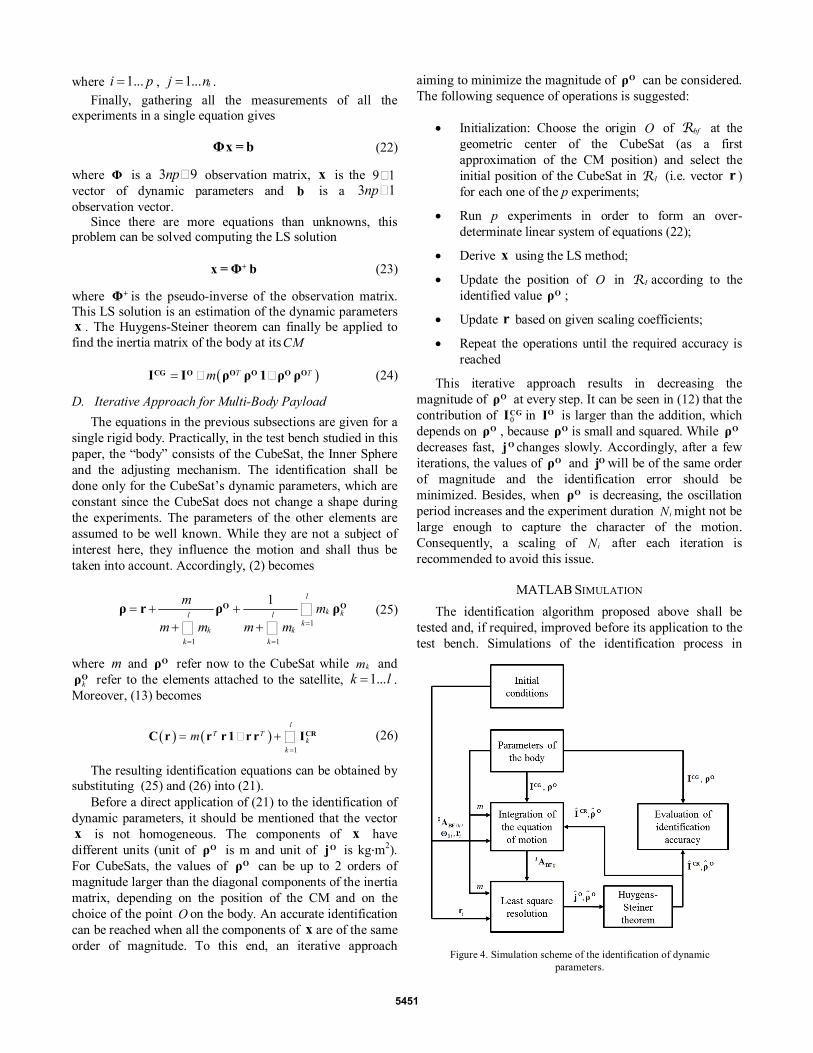
Figure 4. Simulation scheme of the identification of dynamic parameters.

where 1...i p= , 1... ij n= . Finally, gathering all the measurements of all the

experiments in a single equation gives

Φx = b (22)

where Φ is a 3 9np× observation matrix, x is the 9 1× vector of dynamic parameters and b is a 3 1np×observation vector.

Since there are more equations than unknowns, this problem can be solved computing the LS solution

+x =Φ b (23)

where +Φ is the pseudo-inverse of the observation matrix. This LS solution is an estimation of the dynamic parametersx . The Huygens-Steiner theorem can finally be applied to find the inertia matrix of the body at itsCM

( )T Tm= − −CG O O O O OI I ρ ρ 1 ρ ρ (24)

D. Iterative Approach for Multi-Body Payload The equations in the previous subsections are given for a

single rigid body. Practically, in the test bench studied in this paper, the “body” consists of the CubeSat, the Inner Sphere and the adjusting mechanism. The identification shall be done only for the CubeSat’s dynamic parameters, which are constant since the CubeSat does not change a shape during the experiments. The parameters of the other elements are assumed to be well known. While they are not a subject of interest here, they influence the motion and shall thus be taken into account. Accordingly, (2) becomes

1

1 1

1 l

k kl lk

k kk k

m mm m m m =

= =

= + ++ +

∑∑ ∑

O Oρ r ρ ρ (25)

where m and Oρ refer now to the CubeSat while km and kOρ refer to the elements attached to the satellite, 1...k l= .

Moreover, (13) becomes

( ) ( )1

lT T

kk

m=

= − + ∑ CRC r r r 1 r r I (26)

The resulting identification equations can be obtained by substituting (25) and (26) into (21).

Before a direct application of (21) to the identification of dynamic parameters, it should be mentioned that the vector x is not homogeneous. The components of x have different units (unit of Oρ is m and unit of Oj is kg·m2). For CubeSats, the values of Oρ can be up to 2 orders of magnitude larger than the diagonal components of the inertia matrix, depending on the position of the CM and on the choice of the point O on the body. An accurate identification can be reached when all the components of x are of the same order of magnitude. To this end, an iterative approach

aiming to minimize the magnitude of Oρ can be considered. The following sequence of operations is suggested:

• Initialization: Choose the origin O of bfR at the geometric center of the CubeSat (as a first approximation of the CM position) and select the initial position of the CubeSat in IR (i.e. vector r ) for each one of the p experiments;

• Run p experiments in order to form an over-determinate linear system of equations (22);

• Derive x using the LS method;

• Update the position of O in IR according to the identified value Oρ ;

• Update r based on given scaling coefficients;

• Repeat the operations until the required accuracy is reached

This iterative approach results in decreasing the magnitude of Oρ at every step. It can be seen in (12) that the contribution of 0

CGI in OI is larger than the addition, which depends on Oρ , because Oρ is small and squared. While Oρdecreases fast, Oj changes slowly. Accordingly, after a few iterations, the values of Oρ and Oj will be of the same order of magnitude and the identification error should be minimized. Besides, when Oρ is decreasing, the oscillation period increases and the experiment duration iN might not be large enough to capture the character of the motion. Consequently, a scaling of iN after each iteration is recommended to avoid this issue.

MATLAB SIMULATION The identification algorithm proposed above shall be

tested and, if required, improved before its application to the test bench. Simulations of the identification process in

5451

MATLAB are thus used to verify the algorithm efficiency. The MATLAB model consists of two parts: The simulation of the body dynamics and the identification of the dynamic parameters (Fig. 4).

The rotating body dynamics is described by (7). The simulation of the body motion requires to solve this equation to determine the angular position of the body, described by the rotation matrix I

BFA . Finding IBFA emulates data that

will be obtained from the sensors of the test bench during the real experiments.

The part of the MATLAB model, dedicated to the identification of the inertial parameters, is similar to the one that will be used during the real experiments. The accuracy of the identification process can be estimated by comparing the “real” values CRI and Oρ , chosen by the user for the current model run, and the values CRI$ and $ Oρ obtained by the identification process.

E. Simulation of the body motion Equation (7) shall be written in the following form to be

solved by the MATLAB Ordinary Differential Equation (ODE) solver

( )f=y y& , (27)

where y is the vector of unknowns. Equation (7) contains first and second order derivatives of the angular position of the body. Moreover, the angular velocity is not linearly dependent on the sought-for rotation matrix I

BFA . The following solution is proposed to deal with this issue.

Let y to be the vector composed of the components of I

BFA and Iω

[ ]11 21 31 12 22 32 31 32 33 1 2 3TA A A A A A A A A= ω ω ωy (28)

Using (3), the first 9 components of y& can be found from the equation

[ ]×=I I IBF BFA ω A& (29)

Equation (7) can be solved for Iω& , which are the last 3 components of y&

( ) [ ]( )( )1 m−

×= − × −I I CR BF I CR BF I BF IBF I I Iω A I ωA I A ω A g ρ& (30)

Thereby, the equations of motion can be expressed in the form (27) which is required by the ODE solver.

F. Results MATLAB simulations were run for CAD models of 1U

and 3U CubeSats with different dynamic characteristics and initial conditions, represented in Table I and Table III. At the beginning of each experiment, the CubeSat is at rest and the axes of bfR and IR are perfectly aligned.

The scaling coefficients for r and the duration of each experiment, which depends on the magnitude of Oρ derived during the previous iteration, were found empirically and are given in Table II. The sampling time for all iterations is 0.1 sec.

TABLE I. INITIAL CONDITIONS

Experiment number, p 1 2 3 4

Initial offset, r (m)

0.020.020.02

0.020.02

0.02

− −

0.020.020.02

−

0.020.020.02

− −

−

The results of the identification and the corresponding

number of iterations, required to obtain Oρ with an accuracy of 1µm (that is needed to meet disturbing torque requirements) are given in Table 3.

These simulations provide good results in the identification of the CM location (largest error <0.1%) and of the moments of inertia (largest error <1%), but for the accurate identification of the products of inertia some additional measures might be needed. The latter can be explained by the small magnitudes of the products of inertia with respect to other identified values. However, the products of inertia should always be small due to the parallelepiped shape of the satellite. Furthermore, they are not important to the CubeSat balancing.

Based on the conducted simulations of the identification process, better results are obtained when at least 4 experiments are made such that, in each experiment, the geometric center of the CubeSat is located in a different octant of IR . However, further research on the optimization of the identification process shall be done to improve its efficiency.

TABLE II. SCALING COEFFICIENTS

Oρ at the previous iteration (m)

Scaling coefficient for r

Duration of each experiment, Ni (sec)

≥ 0.01 1 5

≥ 0.001 0.5 10

≥ 0.0001 0.1 20

< 0.0001 0.05 25

TABLE III. RESULTS OF SIMULATIONS

1U CubeSat 3U CubeSat

CAD values

Identified values

CAD values

Identified values

O 31ρ (m 10 )−⋅ -0.2560 -0.2558 -1.6393 -1.6398 O 32ρ (m 10 )−⋅ -0.9320 -0.9317 -1.2807 -1.2814 O 33ρ (m 10 )−⋅ -9.9570 -9.9572 17.1741 17.1749 CM 2 3xxI (kgm 10 )−⋅ 1.5460 1.5325 30.6915 30.4716 CM 2 3yyI (kgm 10 )−⋅ 1.5910 1.5797 29.6998 29.4381 CM 2 3zzI (kgm 10 )−⋅ 1.3840 1.3817 4.5775 4.5399 CM 2 3xyI (kgm 10 )−⋅ 0.0090 -0.0087 0.0250 -0.2039 CM 2 3xzI (kgm 10 )−⋅ -0.0070 0.0030 -0.1459 -0.0052 CM 2 3yzI (kgm 10 )−⋅ 0.0060 0.0082 0.0030 0.0021

Number of iterations (Section IV-D)

4 4

5452

V. CONCLUSION A novel concept of an air bearing test bench for CubeSat

ground testing was proposed in this paper. In contrast to existing air-bearing test benches, it allows unlimited 3 DoF rotations of the tested CubeSat while reducing the undesired influences caused by the other mobile elements attached to the CubeSat. Moreover, a dynamic parameter identification method, adapted to the proposed test bench, was presented. This method is mainly based on the sampling of free oscillating motions. Simulation results of dynamic parameter identification for CAD models were presented. Future work will aim at validating the identification method on the assembled test bench with a CubeSat prototype.

REFERENCES [1] M. Swartwout, "The first one hundred CubeSats: a statistical look,"

Journal of Small Satellites, vol. 2, no. 2, pp. 213-233, 2013. [2] J. Kim and B. Agrawal, "Automatic mass balancing of air-bearing-

based three-axis rotational spacecraft simulator," Journal of Guidance, Control, and Dynamics, vol. 32, no. 3, pp. 1005-1017, May-June 2009.

[3] M. A. Peck and A. R. Cavender, "An airbearing-based testbed for momentum-control systems and spacecraft line of sight," Advances in the Astronautical Sciences (American Astronautical Society), pp. 427-446, 2003.

[4] B. N. Agrawal and R. E. Rasmussen, "Air bearing based satellite attitude dynamics simulator for control software research and development," Proc.SPIE, Technologies for Synthetic Environments: Hardware-in-the-Loop Testing, vol. 4366, pp. 204-214, 2001.

[5] C. W. Crowell, Development and analysis of a small satellite attitude determination and control system testbed, Massachusetts, 2011.

[6] R. Fullmer, G. Peterson, W. Holmans, J. Smith, J. Nottingham, S. Anderson, T. Olsen and F. Redd, The development of a small satellite attitude control simulator, Utah State University, Loagan UT.

[7] G. Bisiacchi, J. Prado, L. Reyes, E. Vicente, F. Contreras, M. Mesinas and A. Juarez, "Three-axis air-bearing based platform for small satellite attitude determination and control simulation," Journal of Applied Research and Technology, vol. 3, no. 3, pp. 222-237, 2005.

[8] B. Kim, E. Velenis, P. Kriengsiri and P. Tsiotras, "Designing a low- cost spacecraft simulator," IEEE Control Systems Magazine, pp. 26-37, August 2003.

[9] D. M. Meissner, "A three degrees of freedom test bed for nanosatellite and CubeSat attitude dynamics, determination, and control, " Monterey, California, 2009.

[10] D. Gallardo and R. Bevilacqua, "Six degrees of freedom experimental platform for testing autonomous satellites operations," in 8th International ESA Conference on Guidance, Navigation and Control Systems, Karlovy Vary, 2011.

[11] T. Ustrzycki, R. Lee and H. Chesser, "Spherical air bearing attitude control simulator for nanosatellites," in AIAA Modeling and Simulation Technologies Conference, Portland, Oregon, 2011.

[12] J. L. Schwartz, The distributed spacecraft attitude control system simulator: from design concept to decentralized control, Blacksburg, Virginia, 2004.

[13] W. Khalil and E. Dombre, Modeling, Identification and Control of Robots, CRC Press, 2002.

[14] B. Siciliano, L. Sciavicco, L. Villani and G. Oriolo, Robotics. Modelling, Planning and Control, Springer, 2010.

[15] M. Gautier and S. Briot, "New method for global identification of the joint driven gains of robots using a known payload mass," in IEEE/RSJ International Conference on Intelegent Robots and Systems, San-Francisco, CA, 2011.

[16] C. H. An, C. G. Atkeson and J. M. Hollerbach, "Estimation of inertial parameters of rigid body links of manipulators," Massachusetts Institute of Technology, Artificial Intelligence Laboratory, Massachusetts, 1986.

[17] E. Wilson, C. Lages and R. Mah, "On-line, gyro-based, mass-property identification for thruster-controlled spacecraft using recursive least squares," Proceedings of the 45th IEEE International Midwest Symposium on Curcuits and Systems, August 2002.

[18] M. Gautier and S. Briot, "Dynamic parameter identification of a 6 DOF industrial robot using power model," in IEEE International Conference on Robotics and Automation (ICRA), Karlsruhe, 2013.

[19]

J. L. Schwartz, M. A. Peck and C. D. Hall, "Historical review of air-bearing spacecraft simulators," Journal of Guidance, Control, and Dynamics, vol. 26, no. 14, pp. 513-522, 2003.

[20] P. Wang, J. Yee et F. Hadaegh, "Synchronised rotation of multiple autonomous spacesrafts with rule-based control: experimental study," Journal of Guidance, Control, and Dynamics, vol. 24, n° 12, pp. 352-359, 2001.

[21] The CubeSat Program, CubeSat Design Specification Rev.13, Cal Poly SLO, 2014.

5453