Embed Size (px)
Citation preview
Chair of Software Engineering
Robotics Programming Laboratory
Bertrand MeyerJiwon Shin
Lecture 7: Path Planning
2
Getting to Zurich HB from WEH D4
Tram 6, 7 to Bahnhofstrasse/HB
Tram 10 to Bahnhofplatz/HB
Walk down on Weinbergstrasse to Central then to HB
Walk down on Leonhard-Treppe to Walcheplatz to Walchebrücke to HB
Bike down on Weinbergstrasse to Central, then to HB
...
Each path offers different cost in terms of
Time
Convenience
Crowdedness
Ease
...
Path planning
3
Path planning
Path planning: a collection of discrete motions between a start and a goal
Strategies
Graph search
Covert free space to a connectivity graph
Apply a graph search algorithm to find a path to the goal
Potential field planning
Impose a mathematical function directly on the free space
Follow the gradient of the function to get to the goal
4
Configuration space
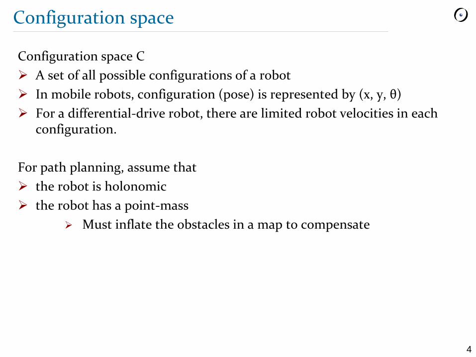
Configuration space C
A set of all possible configurations of a robot
In mobile robots, configuration (pose) is represented by (x, y, θ)
For a differential-drive robot, there are limited robot velocities in each configuration.
For path planning, assume that
the robot is holonomic
the robot has a point-mass
Must inflate the obstacles in a map to compensate
5
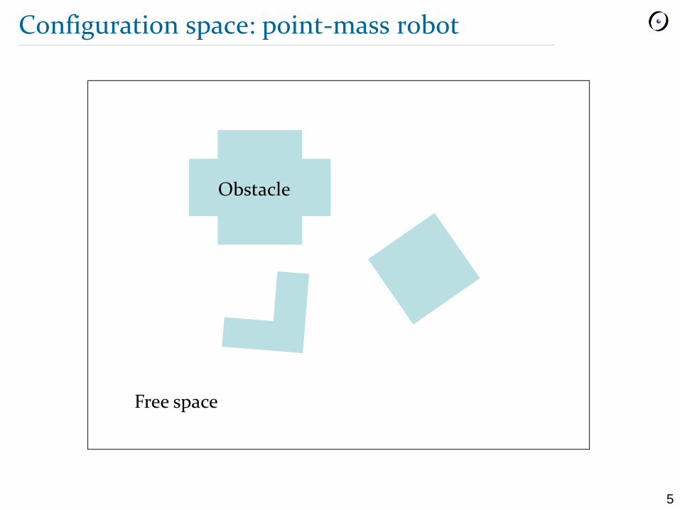
Configuration space: point-mass robot
Free space
Obstacle

6
Configuration space: circular robot
Free space
Obstacle
7
Path planning: graph search
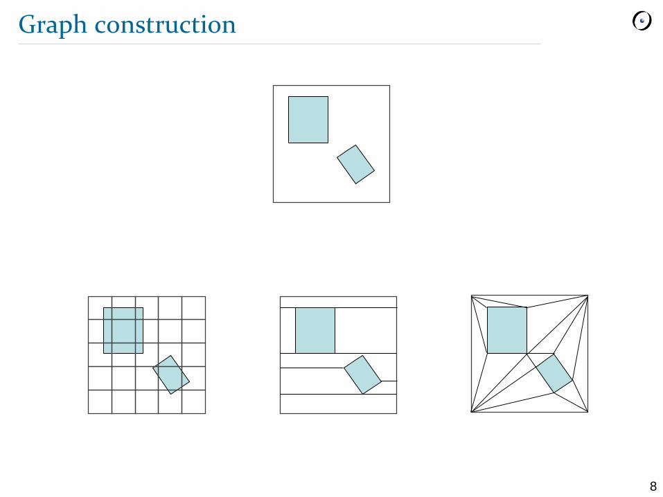
Graph construction
Visibility graph
Voronoi diagram
Exact cell decomposition
Approximate cell decomposition
Graph search
Deterministic graph search
Randomized graph search
8
Graph construction
9
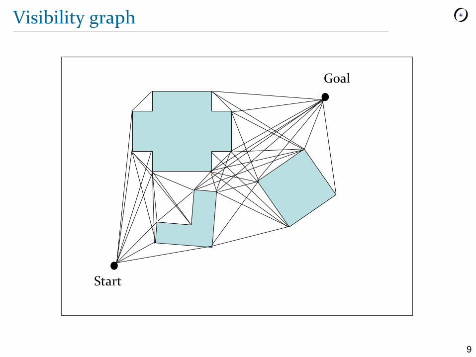
Visibility graph
Goal
Start
10
Visibility graph
Advantages
Optimal path in terms of path length
Simple to implement
Issues
Number of edges and nodes increase with the number of obstacle polygons
Fast in sparse environments, but slow and inefficient in densely populated environments
Resulting path takes the robot as close as possible to obstacles
A modification to the optimal solution is necessary to ensure safety
• Grow obstacles by radius much larger than robot’s radius
• Modify the solution path to be away from obstacles
11
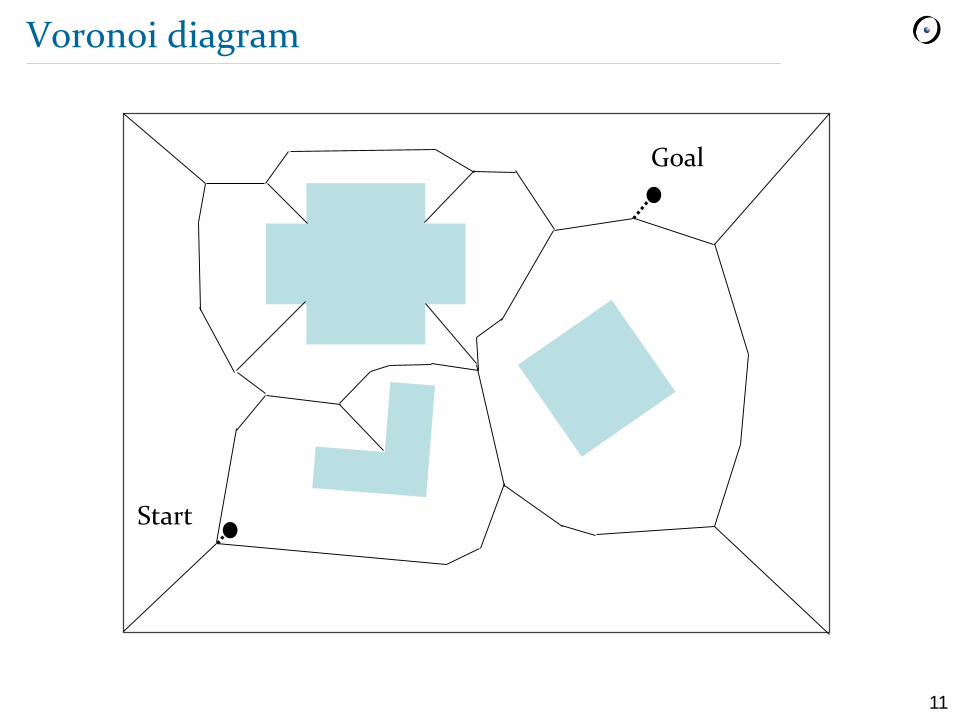
Voronoi diagram
Goal
Start
12
Voronoi diagram
For each point in free space, compute its distance to the nearest obstacle.
At points that are equidistant to two or more obstacles, create ridge points.
Connect the ridge points to create the Voronoi diagram
13
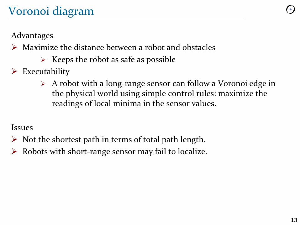
Voronoi diagram
Advantages
Maximize the distance between a robot and obstacles
Keeps the robot as safe as possible
Executability
A robot with a long-range sensor can follow a Voronoi edge in the physical world using simple control rules: maximize the readings of local minima in the sensor values.
Issues
Not the shortest path in terms of total path length.
Robots with short-range sensor may fail to localize.
14
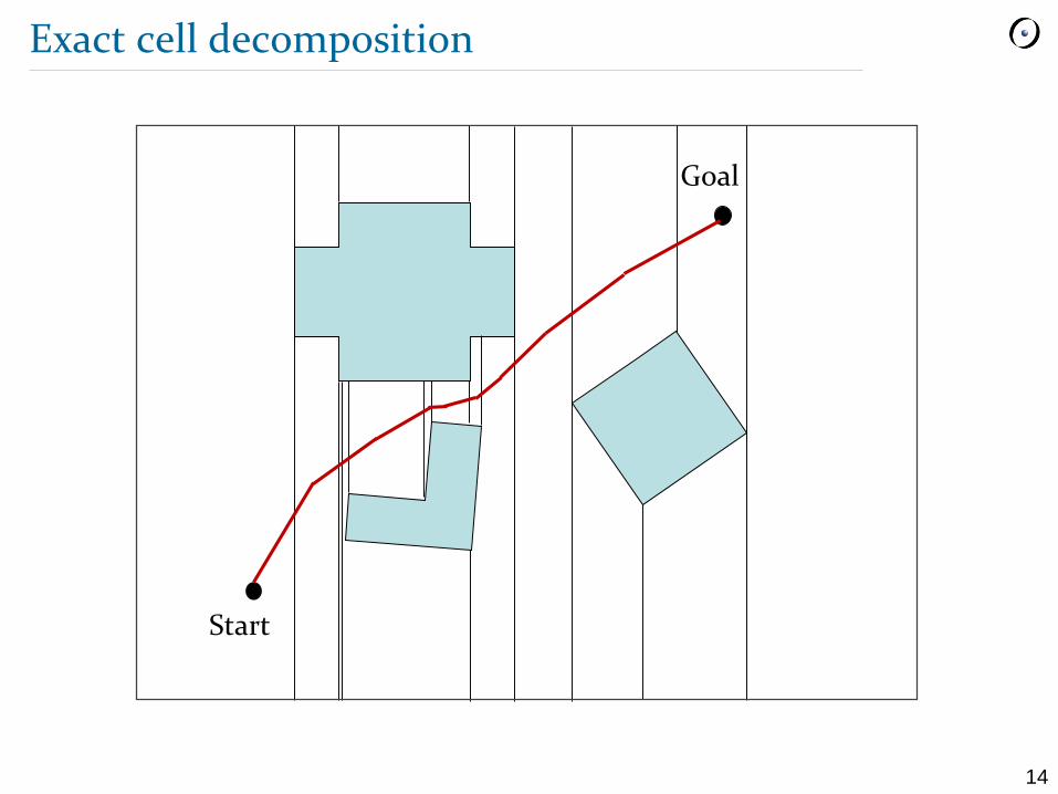
Exact cell decomposition
Goal
Start
15
Exact cell decomposition
Advantages
In a sparse environment, the number of cells is small regardless of actual environment size.
Robots can move around freely within a free cell.
Issues
The number of cells depends on the destiny and complexity of obstacles in the environment
16
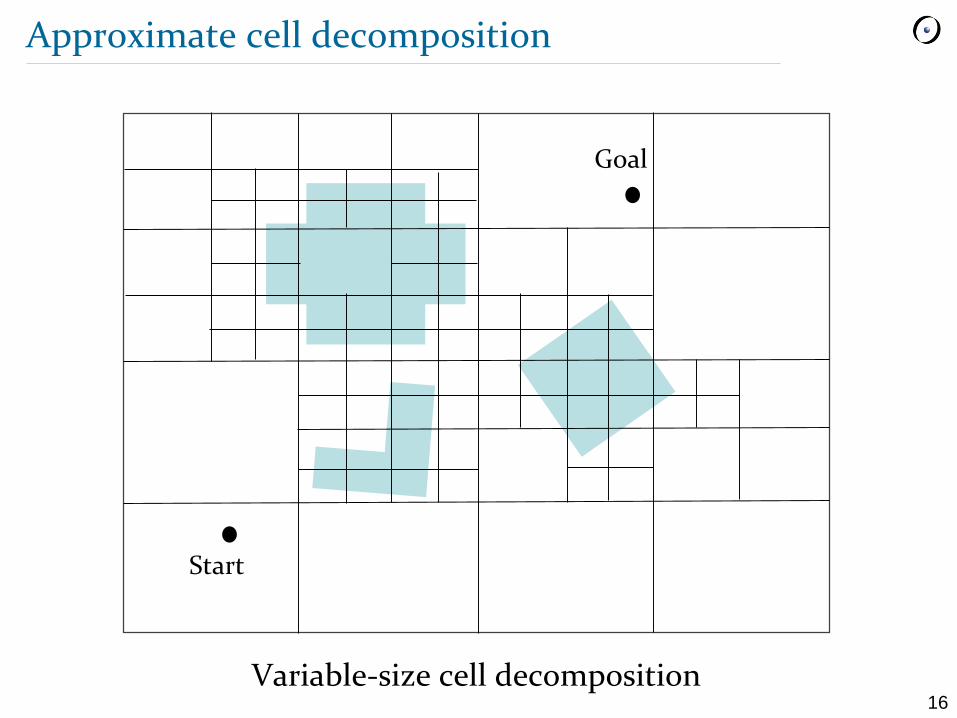
Approximate cell decomposition
Variable-size cell decomposition
Goal
Start
17
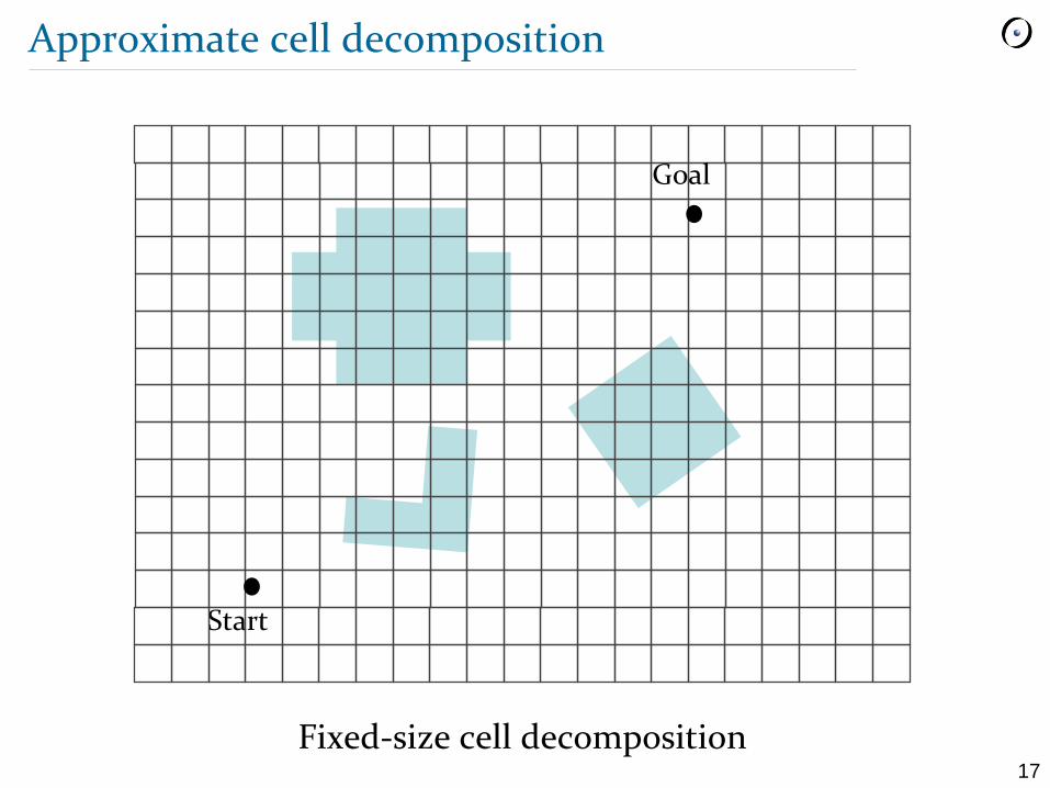
Approximate cell decomposition
Fixed-size cell decomposition
Start
Goal
18
Approximate cell decomposition
Variable-size
Recursively divide the space into rectangles unless
A rectangle is completely occupied or completely free
Stop the recursion when
A path planner can compute a solution, or
A limit on resolution is attained
Fixed-size
Divide the space evenly
The cell size is often independent of obstacles
19
Approximate cell decomposition
Advantages
Low computational complexity
Issues
Narrow passage ways can be lost
20
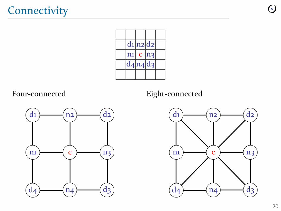
Connectivity
Four-connected Eight-connected
d4 n4
n1
d1
c
n2
d3
n3
d2
n1
n2
c
n4
n3
d1 d2
d4 d3
n1
n2
c
n4
n3
d1 d2
d4 d3
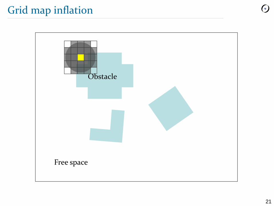
21
Grid map inflation
Free space
Obstacle
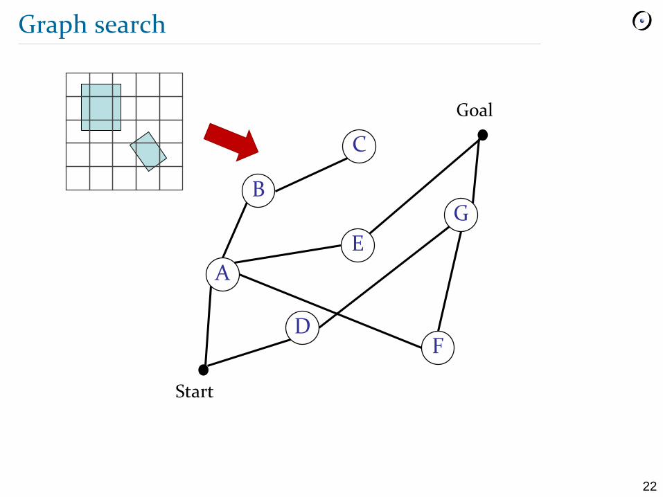
22
Graph search
Goal
Start
A
B
C
D
E
F
G
23
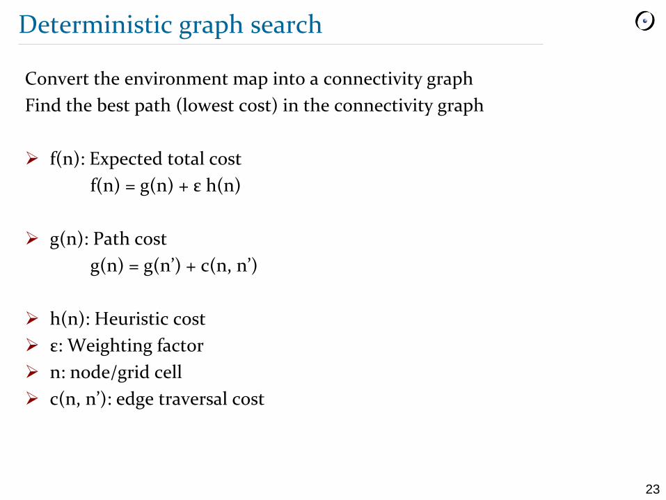
Deterministic graph search
Convert the environment map into a connectivity graph
Find the best path (lowest cost) in the connectivity graph
f(n): Expected total cost
f(n) = g(n) + ε h(n)
g(n): Path cost
g(n) = g(n’) + c(n, n’)
h(n): Heuristic cost
ε: Weighting factor
n: node/grid cell
c(n, n’): edge traversal cost
24
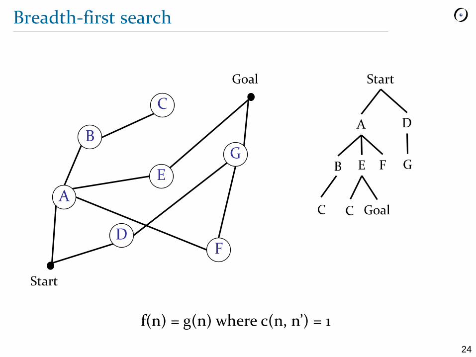
Breadth-first search
Goal
Start
A
B
C
D
E
F
G
Start
A D
B FE G
C C Goal
f(n) = g(n) where c(n, n’) = 1
25
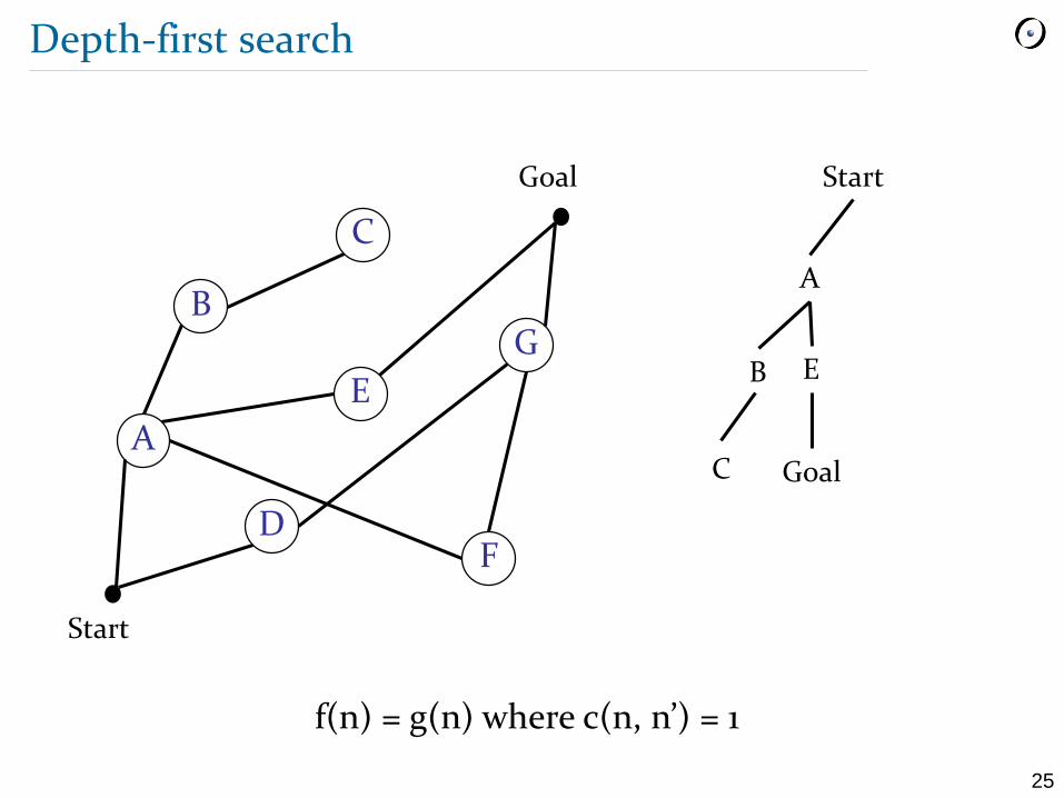
Depth-first search
Goal
Start
A
B
C
D
E
F
G
Start
A
B E
C Goal
f(n) = g(n) where c(n, n’) = 1
26
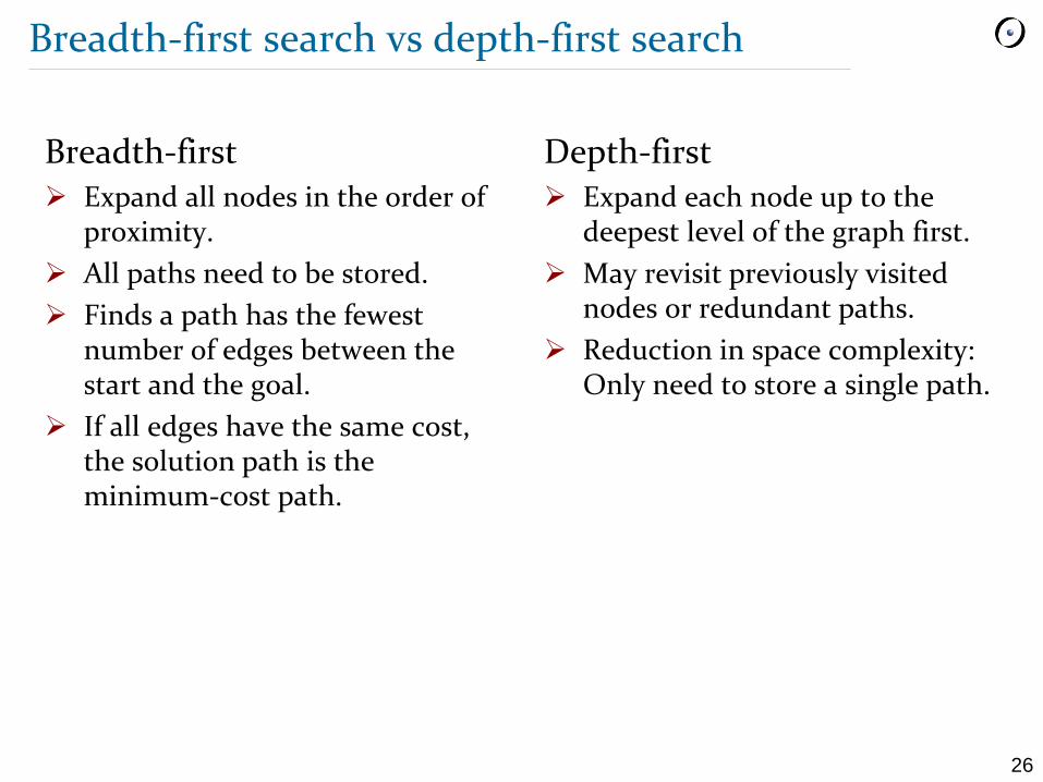
Breadth-first search vs depth-first search
Breadth-first Expand all nodes in the order of
proximity.
All paths need to be stored.
Finds a path has the fewest number of edges between the start and the goal.
If all edges have the same cost, the solution path is the minimum-cost path.
Depth-first Expand each node up to the
deepest level of the graph first.
May revisit previously visited nodes or redundant paths.
Reduction in space complexity: Only need to store a single path.

27
Dijkstra’s algorithm
Goal
Start
A
B
C
D
E
F
G
f(n) = g(n) + 0 * h(n)
Start
A D
B FE G
C Goal
28
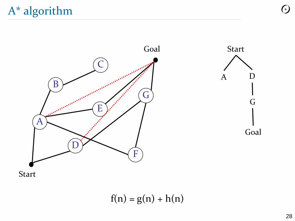
A* algorithm
Goal
Start
A
B
C
D
E
F
G
Start
A D
G
Goal
f(n) = g(n) + h(n)
29
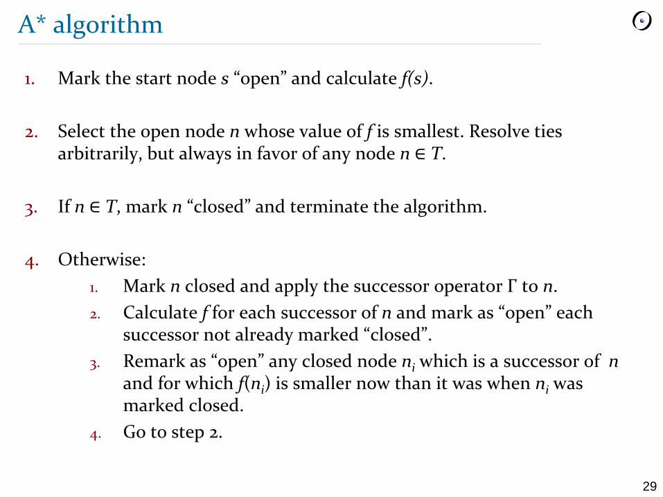
A* algorithm
1. Mark the start node s “open” and calculate f(s).
2. Select the open node n whose value of f is smallest. Resolve ties arbitrarily, but always in favor of any node n ∈ T.
3. If n ∈ T, mark n “closed” and terminate the algorithm.
4. Otherwise:
1. Mark n closed and apply the successor operator Γ to n.
2. Calculate f for each successor of n and mark as “open” each successor not already marked “closed”.
3. Remark as “open” any closed node ni which is a successor of nand for which f(ni) is smaller now than it was when ni was marked closed.
4. Go to step 2.
30
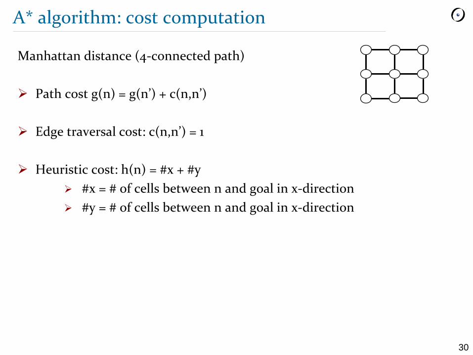
A* algorithm: cost computation
Manhattan distance (4-connected path)
Path cost g(n) = g(n’) + c(n,n’)
Edge traversal cost: c(n,n’) = 1
Heuristic cost: h(n) = #x + #y
#x = # of cells between n and goal in x-direction
#y = # of cells between n and goal in x-direction
31
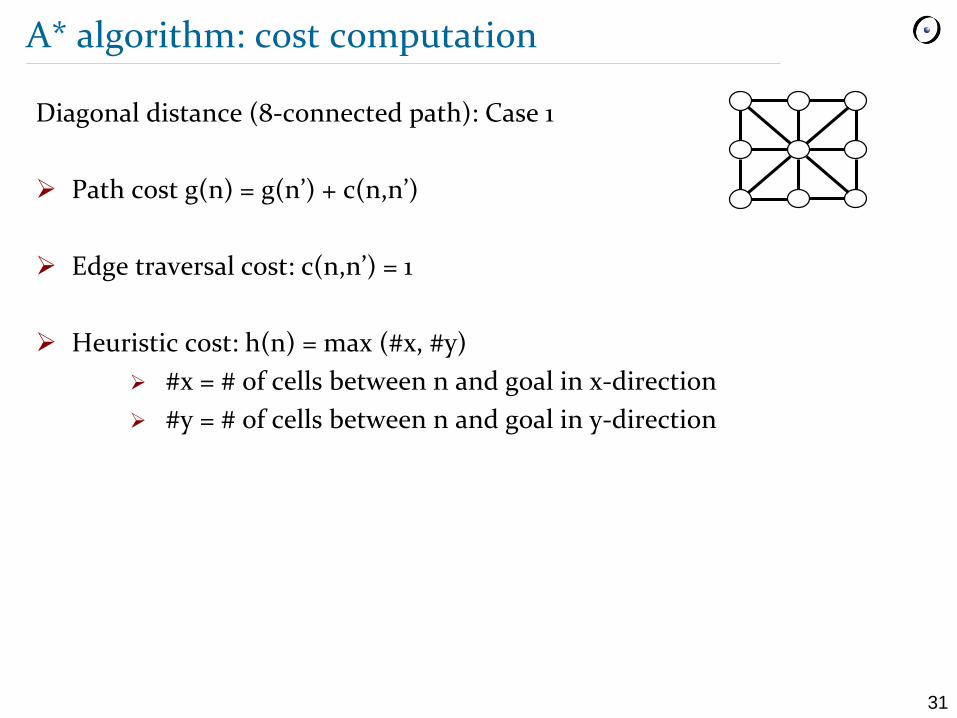
A* algorithm: cost computation
Diagonal distance (8-connected path): Case 1
Path cost g(n) = g(n’) + c(n,n’)
Edge traversal cost: c(n,n’) = 1
Heuristic cost: h(n) = max (#x, #y)
#x = # of cells between n and goal in x-direction
#y = # of cells between n and goal in y-direction
32
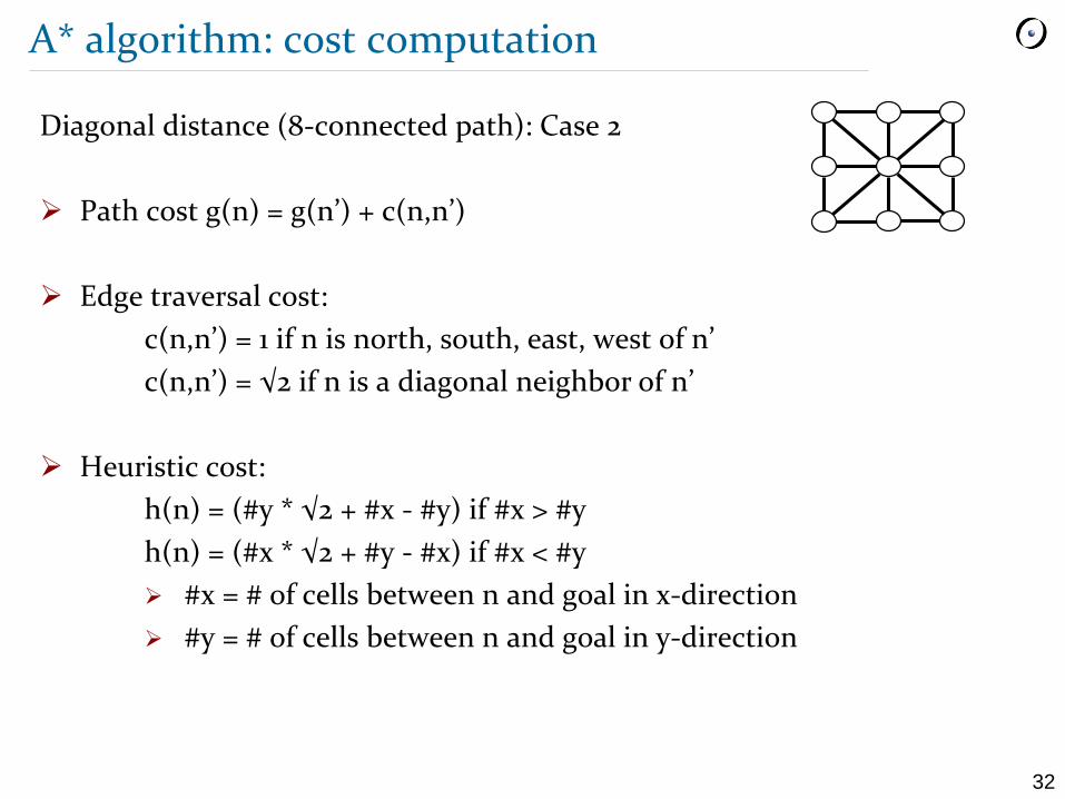
A* algorithm: cost computation
Diagonal distance (8-connected path): Case 2
Path cost g(n) = g(n’) + c(n,n’)
Edge traversal cost:
c(n,n’) = 1 if n is north, south, east, west of n’
c(n,n’) = √2 if n is a diagonal neighbor of n’
Heuristic cost:
h(n) = (#y * √2 + #x - #y) if #x > #y
h(n) = (#x * √2 + #y - #x) if #x < #y
#x = # of cells between n and goal in x-direction
#y = # of cells between n and goal in y-direction
33
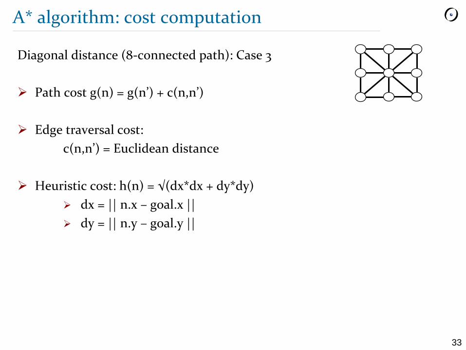
A* algorithm: cost computation
Diagonal distance (8-connected path): Case 3
Path cost g(n) = g(n’) + c(n,n’)
Edge traversal cost:
c(n,n’) = Euclidean distance
Heuristic cost: h(n) = √(dx*dx + dy*dy)
dx = || n.x – goal.x ||
dy = || n.y – goal.y ||
34
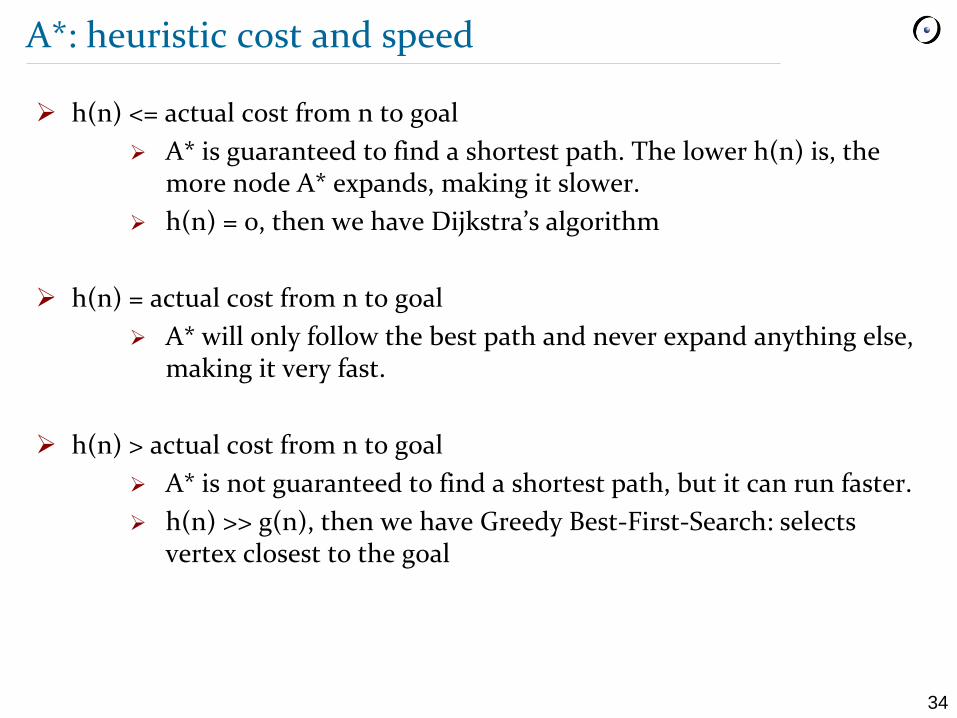
A*: heuristic cost and speed
h(n) <= actual cost from n to goal
A* is guaranteed to find a shortest path. The lower h(n) is, the more node A* expands, making it slower.
h(n) = 0, then we have Dijkstra’s algorithm
h(n) = actual cost from n to goal
A* will only follow the best path and never expand anything else, making it very fast.
h(n) > actual cost from n to goal
A* is not guaranteed to find a shortest path, but it can run faster.
h(n) >> g(n), then we have Greedy Best-First-Search: selects vertex closest to the goal

35
Dijkstra’s algorithm
http://theory.stanford.edu/~amitp/GameProgramming/AStarComparison.html
36
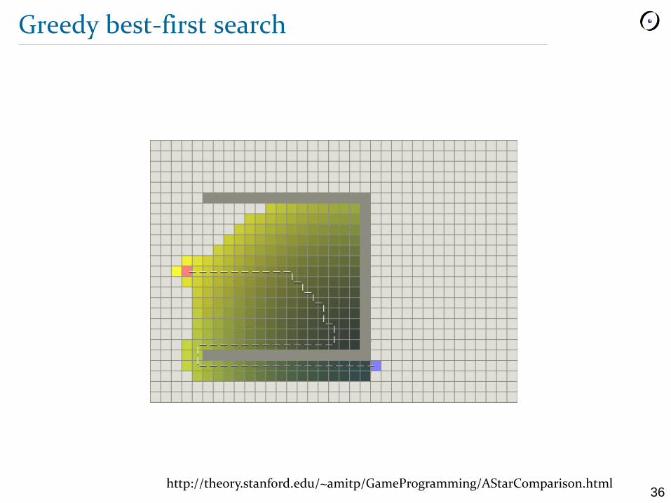
Greedy best-first search
http://theory.stanford.edu/~amitp/GameProgramming/AStarComparison.html
37
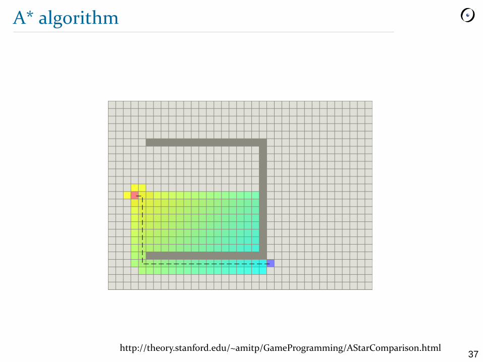
A* algorithm
http://theory.stanford.edu/~amitp/GameProgramming/AStarComparison.html
38
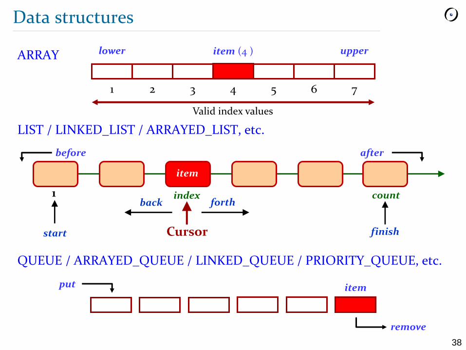
Data structures
ARRAY
LIST / LINKED_LIST / ARRAYED_LIST, etc.
QUEUE / ARRAYED_QUEUE / LINKED_QUEUE / PRIORITY_QUEUE, etc.
Valid index values
lower upper
1
item (4 )
2 3 4 5 6 7
put
remove
item
item
Cursor
forthbackindex count1
finishstart
afterbefore
39
Data structures
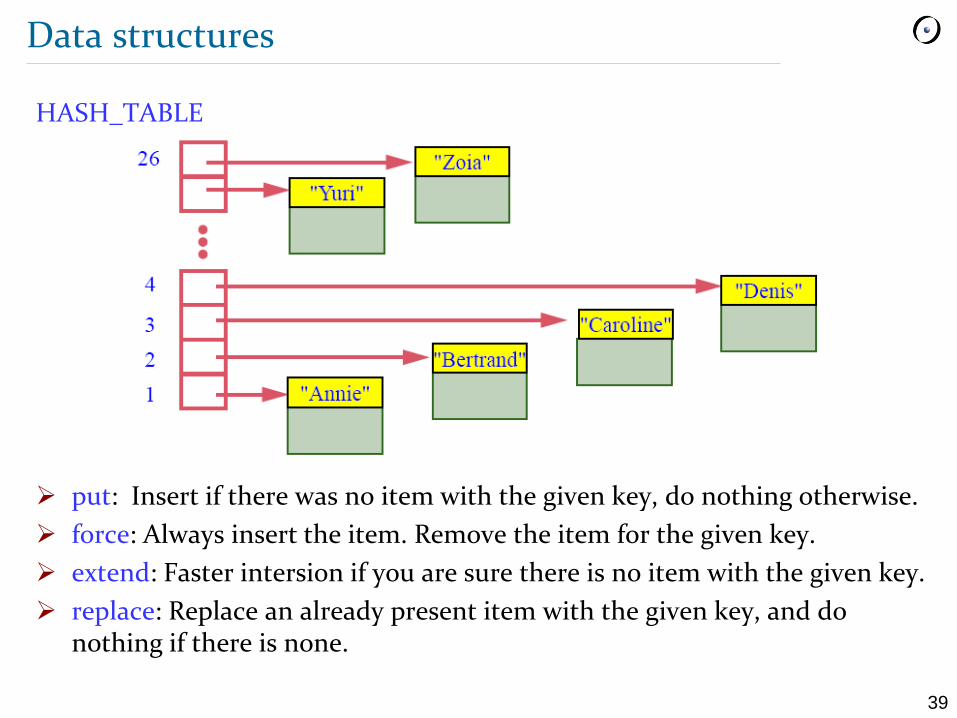
HASH_TABLE
put: Insert if there was no item with the given key, do nothing otherwise.
force: Always insert the item. Remove the item for the given key.
extend: Faster intersion if you are sure there is no item with the given key.
replace: Replace an already present item with the given key, and do nothing if there is none.
40
Randomized graph search
http://msl.cs.uiuc.edu/rrt/gallery_2drrt.html
41
Randomized graph search
1. Initialize a tree.
2. Add nodes to the tree until a termination condition is triggered.
3. During each step:
1. Pick a random configuration qrand in the free space.
2. Compute the tree node qnear closest to qrand
3. Grow an edge (with a fixed length) from qnear to qrand
4. Add the end qnew of the edge if it is collision free
42
Randomized graph search
Advantages
Can address situations in which exhaustive search is not an option.
Issues
Cannot guarantee solution optimality.
Cannot guarantee deterministic completeness.
If there is a solution, the algorithm will eventually find it as the number of nodes added to the tree grows to infinity.
43
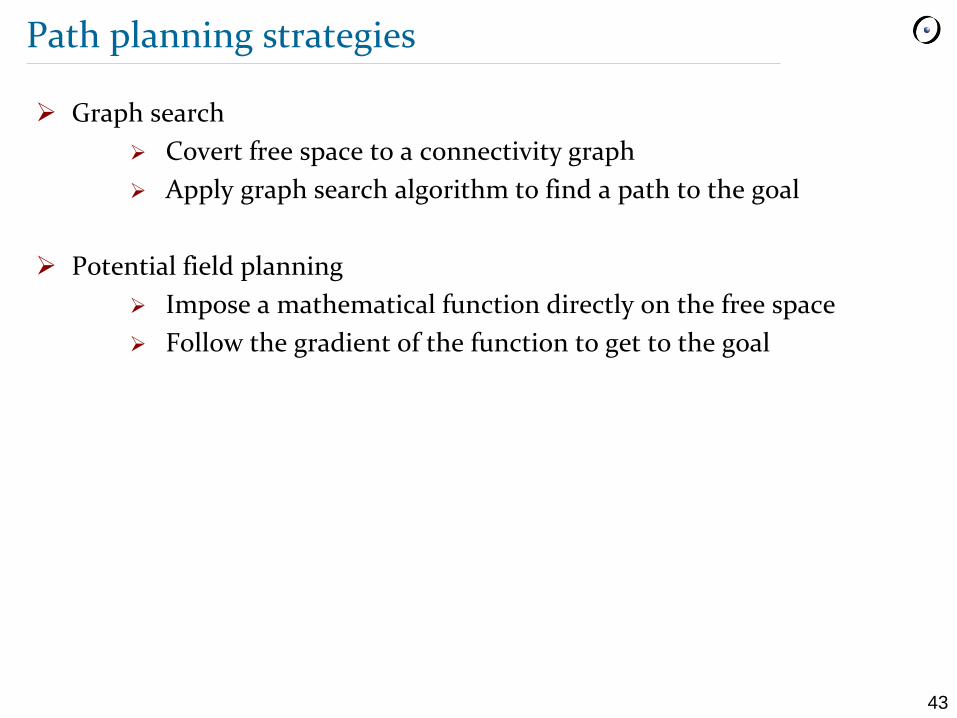
Path planning strategies
Graph search
Covert free space to a connectivity graph
Apply graph search algorithm to find a path to the goal
Potential field planning
Impose a mathematical function directly on the free space
Follow the gradient of the function to get to the goal

44
Potential field
Create a gradient to direct the robot to the goal position
Main idea
Robots are attracted toward the goal.
Robots are repulsed by obstacles.
F(q) = - 𝛻U(q)
F(q): artificial force acting on the robot at the position q = (x, y)
U(q): potential field function
𝛻U(q): gradient vector of U at position q
U(q) = Uattractive(q) + Urepulsive(q)
F(q) = Fattractive(q) + Frepulsive(q) = - 𝛻Uattractive(q) - 𝛻Urepulsive(q)
45
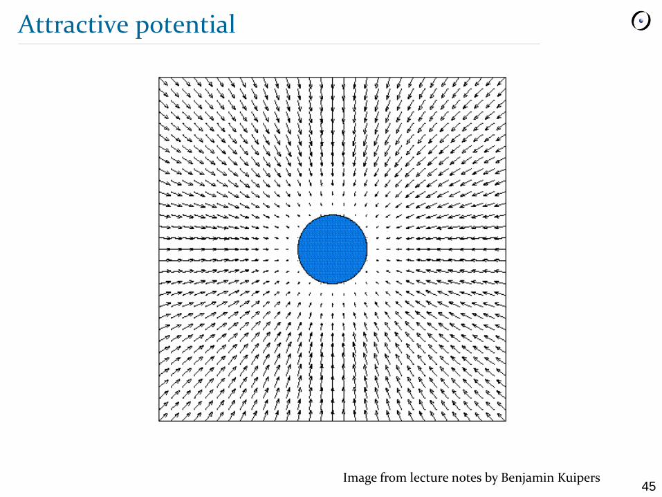
Attractive potential
Image from lecture notes by Benjamin Kuipers

46
Repulsive potential
Image from lecture notes by Benjamin Kuipers
47
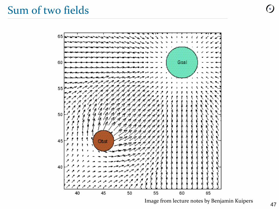
Sum of two fields
Image from lecture notes by Benjamin Kuipers
48
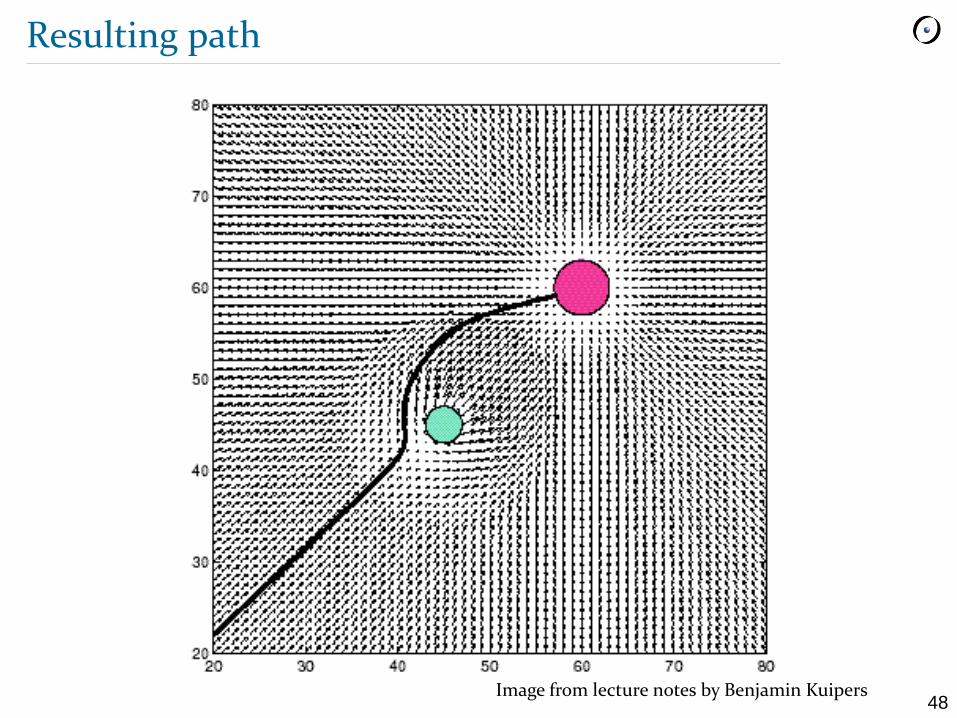
Resulting path
Image from lecture notes by Benjamin Kuipers
49
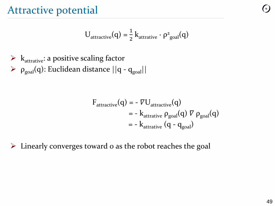
Attractive potential
Uattractive(q) = 1
2kattrative ∙ ρ2
goal(q)
kattrative: a positive scaling factor
ρgoal(q): Euclidean distance ||q - qgoal||
Fattractive(q) = - 𝛻Uattractive(q)
= - kattrative ρgoal(q) 𝛻 ρgoal(q)
= - kattrative (q - qgoal)
Linearly converges toward 0 as the robot reaches the goal
50
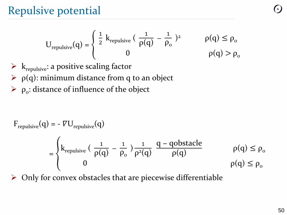
Repulsive potential
Urepulsive(q) =
1
2krepulsive (
1
ρ(q)−
1
ρ0)2 ρ(q) ≤ ρ0
0 ρ(q) > ρ0
krepulsive: a positive scaling factor
ρ(q): minimum distance from q to an object
ρ0: distance of influence of the object
Frepulsive(q) = - 𝛻Urepulsive(q)
= krepulsive (
1
ρ(q)−
1
ρ0)
1
ρ2(q)q − qobstacle
ρ(q)ρ(q) ≤ ρ0
0 ρ(q) ≤ ρ0
Only for convex obstacles that are piecewise differentiable
51
Potential field
Advantages
Both plans the path and determines the control for the robot.
Smoothly guides the robot towards the goal.
Issues
Local minima are dependent on the obstacle shape and size.
Concave objects may lead to several minimal distances, which can cause oscillation