Robotics: Tutorial 3 - MNRLab · Inverse Position Kinematics ... Omar Mahmoud, Eng. Lobna Tarek and Eng. Abdelrahman Ezz Robotics: Tutorial 3 4 / 33. Then get the slope F_(x 0),

Robotics: Tutorial 3Mechatronics Engineering

Dr. Islam Khalil, MSc. Omar Mahmoud, Eng. Lobna Tarekand Eng. Abdelrahman Ezz

German University in CairoFaculty of Engineering and Material Science

October 4, 2016

Dr. Islam Khalil, MSc. Omar Mahmoud, Eng. Lobna Tarek and Eng. Abdelrahman Ezz Robotics: Tutorial 3 1 / 33

Inverse Position Kinematics

Introducing one of the methods available to solve inverseposition kinematics level.

Using one of the most important numerical methods, NewtonRaphson.

It depends on finding a numerical solution of a non-linearequation(s) instead of evaluating the closed form solution.


Newton Raphson - Graphical Approach

Now, For the shown non-linear function:


Starting from Any initial guess,we evaluate the function F (x0) atx0.


Then get the slope F (x0), which when intersect the x-axis, produce(in most cases) a point closer to the rest of the function.


This is done in several iteration.


until it converge to the acceptable error value.


Problems of Newton Raphson

Function diverge away from the root by choosing the wronginitial solution.

Slope = zero at initial solution chosen.


Newton Raphson - Mathematical Approach

Let’s take a look at the mathematics behind this: at the initialguess point (x0)), the first derivative equation, which is the slopeas well:

slope =∆y

∆x=

F (x0)− 0

x0 − x1(1)

F (x0)[x0 − x1] = F (x0) (2)

x0 − x1 =F (x0)

F (x0)(3)

which can be written as:(this is for a single iteration, starting aninitial guess).

x1 = x0 − [F (x0)]−1F (x0)] (4)

In General Form:

xn+1 = xn − [F (xn)]−1F (xn)] (5)

where, n is number of current iteration.Dr. Islam Khalil, MSc. Omar Mahmoud, Eng. Lobna Tarek and Eng. Abdelrahman Ezz Robotics: Tutorial 3 9 / 33

Application of Newton Raphson in Robotics

We will expand this same formula for our application, inrobotics,by changing equation from scalar into matrix and mainlyto be used in the inverse position kinematics problem, where wesearch for the values of (q) joint angles that will make end effectorreach desired goal. Thus,

qn+1 = qn − [∂F

∂q]−1|q=qnF (qn) (6)


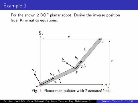
Example 1

For the shown 2 DOF planar robot, Derive the inverse positionlevel Kinematics equations:


Solution

From the forward kinematics (previous tutorial):

x = l1cos(q1) + l2cos(q2) (7)

l1cos(q1) + l2cos(q2)− x = 0→ (f1) (8)

y = l1sin(q1) + l2sin(q2) (9)

l1sin(q1) + l2sin(q2)− y = 0→ (f2) (10)

Relation between joints (q) and position (x) is nonlinear.Therefore, for the inverse kinematics solution, Newton Raphsontechnique is used:We’ll be searching for the values of q1,q2 that satisfy thesefunction, and accordingly end-effector reach its destination:[

q1q2

]1︸︷︷︸

values afterone iteration

=

[q1q2

]0︸︷︷︸

initial values

−

[∂F1∂q1

∂F1∂q2

∂F2∂q1

∂F2∂q2

]−1 [f1(q1, q2)0f2(q1, q2)0

](11)


Evaluation of different elements of equation (11) and Substitution:[q1

q2

]1

=

[q1

q2

]0

−[−l1sin(q1) −l2sin(q2)

l1cos(q1) l2cos(q2)

] ∣∣∣∣−1

q1=q10,q2=q20

[l1cos(q10)+l2cos(q20)−x

l1sin(q10)+l2sin(q20)−y

](12)

This produce values of q1, q2 after 1 iteration, and then thisprocess is repeated for several iterations, in which their valuesconverge to the acceptable values to satisfy the equations f1, f2and these values become the solution of the inverse position levelkinematics.


Inverse Velocity Kinematics

Relation between end effector velocities vector and Joints velocitiesvector is linear, and we can get q1 and q2 from position kinematics.The solution is:

q = J−1(q)X (13)

q → Joints velocities vector.

J−1(q) → Inverse of Jacobian Matrix.can be calculated using MATLAB.

x → end effector velocities vector.


Inverse Acceleration Kinematics

Relation between end effector acceleration vector and Jointsacceleration vector is Affine (Linear relation with a shift) and wecan get q1 and q2 from velocity kinematics.

q = J−1(q)[X − J(q)q] (14)

q → Joints acceleration vector.

J−1(q) → Inverse of Jacobian Matrix.can be calculated using MATLAB.

X → end effector acceleration vector.

J(q) → rate of change of Jacobian matrix.

q → joints velocities vector.


Example 2

For the shown 3 DOF non-planar robot, Derive the equations forposition, velocity and acceleration level Kinematics equations(Forward and inverse):


The Forward Position Level Kinematic

First Step: Assign the frames: Newtonian Frame and local framesat each joint.


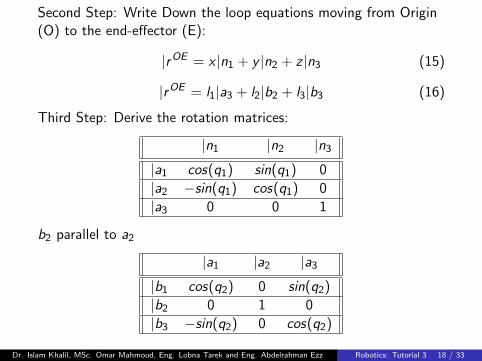
Second Step: Write Down the loop equations moving from Origin(O) to the end-effector (E):

|rOE = x |n1 + y |n2 + z |n3 (15)

|rOE = l1|a3 + l2|b2 + l3|b3 (16)

Third Step: Derive the rotation matrices:

|n1 |n2 |n3|a1 cos(q1) sin(q1) 0

|a2 −sin(q1) cos(q1) 0

|a3 0 0 1

b2 parallel to a2

|a1 |a2 |a3|b1 cos(q2) 0 sin(q2)

|b2 0 1 0

|b3 −sin(q2) 0 cos(q2)


where,|a1 = cos(q1)|n1 + sin(q1)|n2 (17)

|a2 = −sin(q1)|n1 + cos(q1)|n2 (18)

|a3 = |n3 (19)

For second frame, (with respect to first frame)

|b1 = cos(q2)|a1 + sin(q2)|a3 (20)

|b2 = |a2 (21)

|b3 = −sin(q2)|a1 + cos(q2)|a3 (22)

(with respect to Newtonian frame),From equation (18) and (21):

|b2 = −sin(q1)|n1 + cos(q1)|n2 (23)

From equation (17),(19) and (22):

|b3 = −sin(q2)cos(q1)|n1 − sin(q2)sin(q1)|n2 + cos(q2)|n3 (24)


Substituting equations (19),(23) and (24) in (15), and equatingboth sides of the equation (15) and (16):

|rOE = l1|n3 − l2sin(q1)|n1 + l2cos(q1)|n2− l3sin(q2)cos(q1)|n1 − l3sin(q2)sin(q1)|n2 + l3cos(q2)|n3 (25)

x |n1 + y |n2 + z |n3 = l1|n3 − l2sin(q1)|n1 + l2cos(q1)|n2− l3sin(q2)cos(q1)|n1 − l3sin(q2)sin(q1)|n2 + l3cos(q2)|n3 (26)

Taking common factors for the right side of the equation:

x |n1 + y |n2 + z |n3 = (−l2sin(q1)− l3sin(q2)cos(q1))|n1+

(l2cos(q1)− l3sin(q2)sin(q1))|n2 + (l1 + l3cos(q2))|n3 (27)


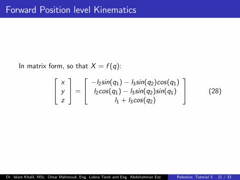
Forward Position level Kinematics

In matrix form, so that X = f (q): xyz

=

−l2sin(q1)− l3sin(q2)cos(q1)l2cos(q1)− l3sin(q2)sin(q1)

l1 + l3cos(q2)

(28)


Inverse Position Level Kinematic

Using the Newton Raphson technique:

q1q2l3

n+1

=

q1q2l3

n

−

∂F1∂q1

∂F1∂q2

∂F1∂l3

∂F2∂q1

∂F2∂q2

∂F2∂l3

∂F3∂q1

∂F3∂q2

∂F3∂l3

−1

q1=q1nq2=q2nL3=L3n

f1(q1, q2, l3)nf2(q1, q2, l3)nf3(q1, q2, l3)n

(29)and the functions are (from forward kinematics):−l2sin(q1)− l3sin(q2)cos(q1)− x = 0→ (f1)l2cos(q1)− l3sin(q2)sin(q1)− y = 0→ (f2)l1 + l3cos(q2)− z = 0→ (f3)


By Substitution/ Evaluation of different elements of this equation: q1q2l3

1

=

q1q2l3

0

−

[−l2cos(q1) + l3sin(q2)sin(q1) −l3cos(q2)cos(q1) −sin(q2)cos(q1)−l2sin(q1)− l3sin(q2)cos(q1) −l3cos(q2)sin(q1) −sin(q2)sin(q1)

0 −l3sin(q2) cos(q2)

] ∣∣∣∣∣−1

q1 = q10q2 = q20l3 = l30 −l2sin(q1)− l3sin(q2)cos(q1)− x

l2cos(q1)− l3sin(q2)sin(q1)− yl1 + l3cos(q2)− z

(30)

This produce values of q1, q2 and L3 after 1 iteration, and thenthis process is repeated for several iterations, in which their valuesconverge to the acceptable values to satisfy the equations f1, f2and f3 and these values become the solution of the inverse positionlevel kinematics.


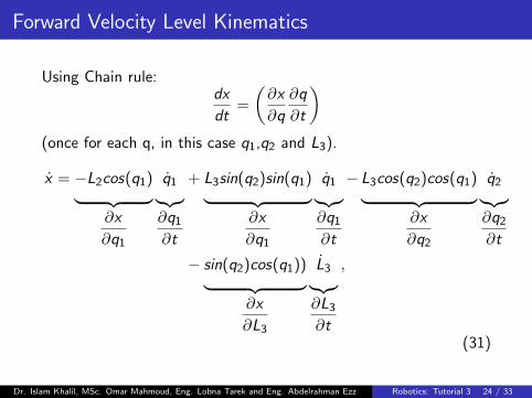
Forward Velocity Level Kinematics

Using Chain rule:dx

dt=

(∂x

∂q

∂q

∂t

)(once for each q, in this case q1,q2 and L3).

x = −L2cos(q1)︸︷︷︸∂x

∂q1

q1︸︷︷︸∂q1∂t

+ L3sin(q2)sin(q1)︸︷︷︸∂x

∂q1

q1︸︷︷︸∂q1∂t

− L3cos(q2)cos(q1)︸︷︷︸∂x

∂q2

q2︸︷︷︸∂q2∂t

− sin(q2)cos(q1))︸︷︷︸∂x

∂L3

L3︸︷︷︸∂L3∂t

,

(31)


Similarly for y ,

y = −L2sin(q1)︸︷︷︸∂y

∂q1

q1︸︷︷︸∂q1∂t

− L3sin(q2)cos(q1)︸︷︷︸∂y

∂q1

q1︸︷︷︸∂q1∂t

− L3cos(q2)sin(q1)︸︷︷︸∂y

∂q2

q2︸︷︷︸∂q2∂t

+ sin(q2)sin(q1)︸︷︷︸∂y

∂L3

L3︸︷︷︸∂L3∂t

,

(32)Similarly for z ,

z = −L3sin(q2)︸︷︷︸∂z

∂q2

q2︸︷︷︸∂q2∂t

+ cos(q2)︸︷︷︸∂x

∂L3

L3︸︷︷︸∂L3∂t

, (33)


Place forward velocity level kinematics equation (31),(32) and (33)in a matrix form so that X = J(q)q: x

yz

=

−L2cq1 + L3sq2sq1 −L3cq2cq1 −sq2cq1−L2sq1 − L3sq2cq1 −L3cq2sq1 −sq2sq1

0 −L3sq2 cq2

q1q2L3

(34)


Inverse Velocity Level Kinematics

Place in q = J−1(q)X :

q1q2L3

=

−L2cq1 + L3sq2sq1 −L3cq2cq1 −sq2cq1−L2sq1 − L3sq2cq1 −L3cq2sq1 −sq2sq1

0 −L3sq2 cq2

−1 xyz

(35)

The inverse of Jacobian Matrix can be calculated using MATLAB.


Forward Acceleration Level Kinematics

Using the chain rule: dxdt =

(∂x∂q

∂q∂t + ∂x

∂q∂q∂t

)x = L2sin(q1)q1

︸︷︷︸∂x

∂q1

q1

︸︷︷︸∂q1

∂t

− L2cos(q1)

︸︷︷︸∂x

∂q1

q1

︸︷︷︸∂q1

∂t

+ L3cos(q2)sin(q1)q1

︸︷︷︸∂x

∂q2

q2

︸︷︷︸∂q2

∂t

+ L3sin(q2)cos(q1)q1

︸︷︷︸∂x

∂q1

q1

︸︷︷︸∂q1

∂t

+ L3sin(q2)sin(q1)

︸︷︷︸∂x

∂q1

q1

︸︷︷︸∂q1

∂t

+ sin(q2)sin(q1)q1

︸︷︷︸∂x

∂l3

L3

︸︷︷︸∂l3

∂t

+ L3cos(q2)sin(q1)q2

︸︷︷︸∂x

∂q1

q1

︸︷︷︸∂q1

∂t

+ L3sin(q2)cos(q1)q2

︸︷︷︸∂x

∂q2

q2

︸︷︷︸∂q2

∂t

− L3cos(q2)cos(q1)

︸︷︷︸∂x

∂q2

q2

︸︷︷︸∂q2

∂t

− cos(q2)cos(q1)q2

︸︷︷︸∂x

∂l3

L3

︸︷︷︸∂l3

∂t

+ L3sin(q2)sin(q1)

︸︷︷︸∂x

∂q1

q1

︸︷︷︸∂q1

∂t

− L3cos(q2)cos(q1)

︸︷︷︸∂x

∂q2

q2

︸︷︷︸∂q2

∂t

− sin(q2)cos(q1)

︸︷︷︸∂x

∂ l3

L3

︸︷︷︸∂ l3

∂t

,

(36)


y =−L2cos(q1)q1

︸︷︷︸∂y

∂q1

q1

︸︷︷︸∂q1

∂t

− L2sin(q1)

︸︷︷︸∂y

∂q1

q1

︸︷︷︸∂q1

∂t

+ L3sin(q2)sin(q1)q1

︸︷︷︸∂y

∂q1

q1

︸︷︷︸∂q1

∂t

− L3cos(q2)cos(q1)q1

︸︷︷︸∂y

∂q2

q2

︸︷︷︸∂q2

∂t

− L3sin(q2)cos(q1)

︸︷︷︸∂y

∂q1

q1

︸︷︷︸∂q1

∂t

− sin(q2)cos(q1)q1

︸︷︷︸∂y

∂l3

L3

︸︷︷︸∂l3

∂t

− L3cos(q2)cos(q1)q2

︸︷︷︸∂y

∂q1

q1

︸︷︷︸∂q1

∂t

+ L3sin(q2)sin(q1)q2

︸︷︷︸∂y

∂q2

q2

︸︷︷︸∂q2

∂t

− L3cos(q2)sin(q1)

︸︷︷︸∂y

∂q2

q2

︸︷︷︸∂q2

∂t

− cos(q2)sin(q1)q2

︸︷︷︸∂y

∂l3

L3

︸︷︷︸∂l3

∂t

− L3sin(q2)cos(q1)

︸︷︷︸∂y

∂q1

q1

︸︷︷︸∂q1

∂t

− L3cos(q2)sin(q1)

︸︷︷︸∂y

∂q2

q2

︸︷︷︸∂q2

∂t

− sin(q2)sin(q1)

︸︷︷︸∂y

∂ l3

L3

︸︷︷︸∂ l3

∂t

,

(37)


z = −L3cos(q2)q2

︸︷︷︸∂z

∂q2

q2

︸︷︷︸∂q2

∂t

− L3sin(q2)

︸︷︷︸∂z

∂q2

q2

︸︷︷︸∂q2

∂t

− sin(q2)q2

︸︷︷︸∂z

∂l3

L3

︸︷︷︸∂l3

∂t

− L3sin(q2)

︸︷︷︸∂z

∂q2

q2

︸︷︷︸∂q2

∂t

+ cos(q2)

︸︷︷︸∂z

∂ l3

L3

︸︷︷︸∂ l3

∂t

,

(38)


Forward Acceleration Kinematics Solution: Place equation(36),(37) and (38) in a matrix form so that X = J(q)q + J(q)q. x

y

z

=

−L2c(q1)+L3s(q2)s(q1) −L3c(q2)c(q1) −s(q2)c(q1)

−L2s(q1)−L3s(q2)c(q1) −L3c(q2)s(q1) −s(q2)s(q1)

0 −L3s(q2) c(q2)

q1

q2

L3

+

L2sq1 q1+L3sq2cq1 q1+L3cq2sq1 q2+L3sq2sq1 L3cq2sq1 q1+L3sq2cq1 q2−L3cq2cq1 sq2sq1 q1−cq2cq1 q2

−L2cq1 q1+L3sq2sq1 q1−L3cq2cq1 q2−L3sq2cq1 −L3cq2cq1 q1+L3sq2cq2 q2−L3cq2sq1 −sq2cq1 q1−cq2sq1 q2

0 −L3cq2 q2−L3sq2 −sq2 q2

q1

q2

L3

(39)


Inverse Acceleration Level Kinematics

The inverse acceleration kinematics solution is:

q = J−1(q)[X − J(q)q]

where, J−1(q) Inverse of Jacobian Matrix can be calculated usingMATLAB.


Any Questions ?Thank you


Documents

Robotics: Tutorial 3 - MNRLab · Inverse Position Kinematics ... Omar Mahmoud, Eng. Lobna Tarek and Eng. Abdelrahman Ezz Robotics: Tutorial 3 4 / 33. Then get the slope F_(x 0),