Embed Size (px)
Citation preview
Springer Handbook of Robotics
Siciliano, Khatib (Eds.) · ©Springer 2008 1
287
Robots with F13. Robots with Flexible Elements
Alessandro De Luca, Wayne Book
Design issues, dynamic modeling, trajectory plan-ning, and feedback control problems are presentedfor robot manipulators having components withmechanical flexibility, either concentrated at thejoints or distributed along the links. The chapter isdivided accordingly in two main parts. Similaritiesor differences between the two types of flexibilityare pointed out wherever appropriate.
For robots with flexible joints, the dynamicmodel is derived in detail by following a Lagrangianapproach and possible simplified versions arediscussed. The problem of computing the nominaltorques that produce a desired robot motion is thensolved. Regulation and trajectory tracking tasksare addressed by means of linear and nonlinearfeedback control designs.
For robots with flexible links, relevant fac-tors that lead to the consideration of distributedflexibility are analyzed. Dynamic models are pre-sented, based on the treatment of flexibilitythrough lumped elements, transfer matrices, orassumed modes. Several specific issues are thenhighlighted, including the selection of sensors,
13.1 Robots with Flexible Joints .................... 28813.1.1 Dynamic Modeling ....................... 28913.1.2 Inverse Dynamics ......................... 29313.1.3 Regulation Control ....................... 29613.1.4 Trajectory Tracking ....................... 30113.1.5 Further Reading ........................... 305
13.2 Robots with Flexible Links ..................... 30613.2.1 Design Issues ............................... 30613.2.2 Modeling of Flexible Link Arms ...... 30813.2.3 Control........................................ 31213.2.4 Further Reading ........................... 316
References .................................................. 317
the model order used for control design, and thegeneration of effective commands that reduceor eliminate residual vibrations in rest-to-restmaneuvers. Feedback control alternatives arefinally discussed.
In each of the two parts of this chapter,a section is devoted to the illustration of theoriginal references and to further readings on thesubject.
The standard assumption underlying robot kinematics,dynamics, and control design is that manipulators con-sist only of rigid bodies (links and motion transmissioncomponents). This is, however, an ideal situation thatmay be considered valid only for slow motion and smallinteracting forces. In practice, mechanical flexibility inrobot manipulators is present for two main reasons: theuse of compliant transmission elements and the reduc-tion of the mass of the moving links through the useof lightweight material and slender design. These twokinds of flexibility introduce static and dynamic deflec-tions between the position of the driving actuators andthe position of the manipulator end-effector. If flexi-bility is not taken into account when considering robot
design and control, a degradation of the overall expectedperformance of the robot typically occurs.
From a modeling point of view, flexibility can be as-sumed as concentrated at the robot joints or distributed(in different ways) along the robot links. The dynamicmodeling steps are similar, with the need to introduceadditional generalized coordinates besides those usedto describe the rigid motion of the robot arm. How-ever, the properties of the resulting models are quitedifferent from a control point of view. Therefore, thecase of robots with flexible joints and of robots withflexible links are presented in this chapter mostly asseparate items, pointing out similarities or structuraldifferences wherever appropriate. For both classes of
PartB
13
Springer Handbook of Robotics
Siciliano, Khatib (Eds.) · ©Springer 20081
288 Part B Robot Structures
flexible robots, the relevant design issues, dynamic mod-eling, inverse dynamics algorithms, and control laws forset-point regulation and trajectory tracking will be dis-cussed. Indeed, joint and link flexibilities may be present(and dynamically interact) at the same time. Many of
the presented results can be extended to this case aswell.
In the following, it is assumed that the reader isalready familiar with basic issues on kinematics, dy-namics, and control of rigid robots (Chaps. 1, 2, 6).
13.1 Robots with Flexible Joints
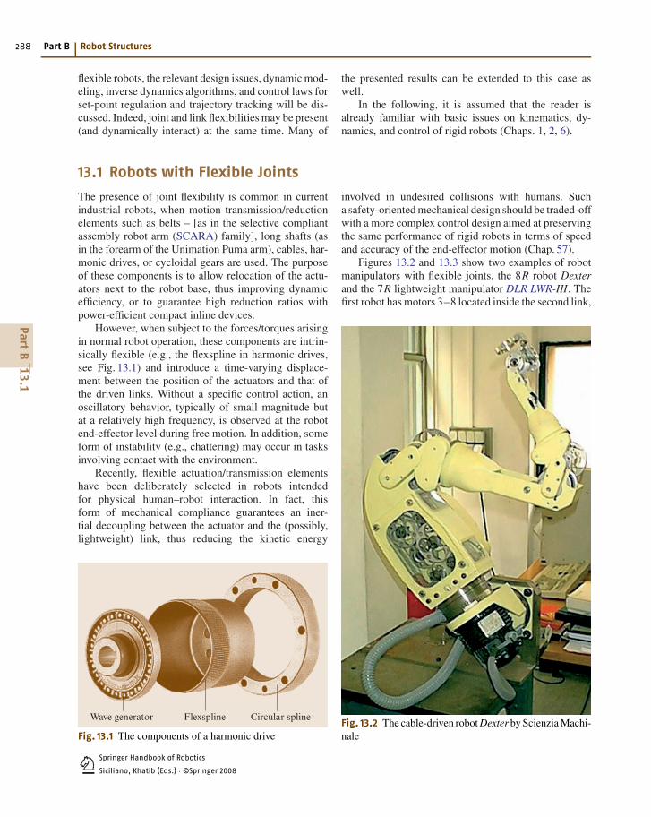
The presence of joint flexibility is common in currentindustrial robots, when motion transmission/reductionelements such as belts – [as in the selective compliantassembly robot arm (SCARA) family], long shafts (asin the forearm of the Unimation Puma arm), cables, har-monic drives, or cycloidal gears are used. The purposeof these components is to allow relocation of the actu-ators next to the robot base, thus improving dynamicefficiency, or to guarantee high reduction ratios withpower-efficient compact inline devices.
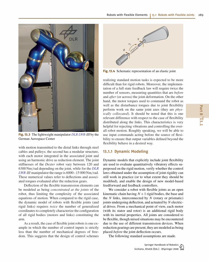
However, when subject to the forces/torques arisingin normal robot operation, these components are intrin-sically flexible (e.g., the flexspline in harmonic drives,see Fig. 13.1) and introduce a time-varying displace-ment between the position of the actuators and that ofthe driven links. Without a specific control action, anoscillatory behavior, typically of small magnitude butat a relatively high frequency, is observed at the robotend-effector level during free motion. In addition, someform of instability (e.g., chattering) may occur in tasksinvolving contact with the environment.
Recently, flexible actuation/transmission elementshave been deliberately selected in robots intendedfor physical human–robot interaction. In fact, thisform of mechanical compliance guarantees an iner-tial decoupling between the actuator and the (possibly,lightweight) link, thus reducing the kinetic energy
Wave generator Flexspline Circular spline
Fig. 13.1 The components of a harmonic drive
involved in undesired collisions with humans. Sucha safety-oriented mechanical design should be traded-offwith a more complex control design aimed at preservingthe same performance of rigid robots in terms of speedand accuracy of the end-effector motion (Chap. 57).
Figures 13.2 and 13.3 show two examples of robotmanipulators with flexible joints, the 8R robot Dexterand the 7R lightweight manipulator DLR LWR-III. Thefirst robot has motors 3–8 located inside the second link,
Fig. 13.2 The cable-driven robot Dexter by Scienzia Machi-nale
PartB
13.1
Springer Handbook of Robotics
Siciliano, Khatib (Eds.) · ©Springer 2008 1
Robots with Flexible Elements 13.1 Robots with Flexible Joints 289
Fig. 13.3 The lightweight manipulator DLR LWR-III by theGerman Aerospace Center
with motion transmitted to the distal links through steelcables and pulleys; the second has a modular structure,with each motor integrated in the associated joint andusing an harmonic drive as reduction element. The jointstiffnesses of the Dexter robot vary between 120 and6300 Nm/rad depending on the joint, while for the DLRLWR-III manipulator the range is 6000–15 000 Nm/rad.These numerical values refer to deflections and associ-ated torques evaluated after the reduction gears.
Deflection of the flexible transmission elements canbe modeled as being concentrated at the joints of therobot, thus limiting the complexity of the associatedequations of motion. When compared to the rigid case,the dynamic model of robots with flexible joints (andrigid links) requires twice the number of generalizedcoordinates to completely characterize the configurationof all rigid bodies (motors and links) constituting thearm.
As a result, the case of flexible joint robots is one ex-ample in which the number of control inputs is strictlyless than the number of mechanical degrees of free-dom. This suggests that the design of control schemes
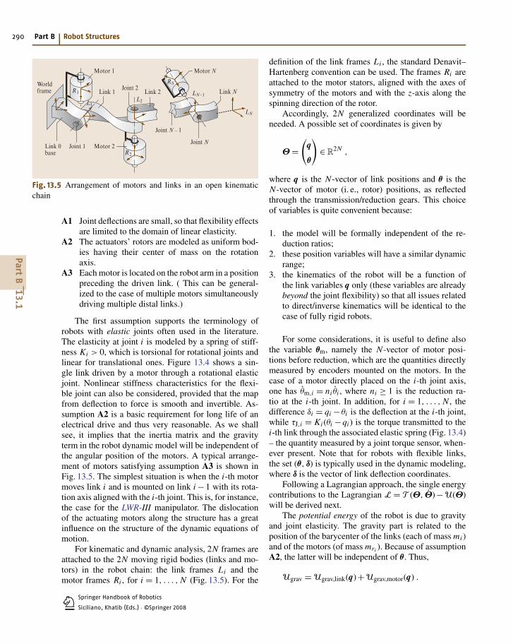
q
θ
τJ
Fig. 13.4 Schematic representation of an elastic joint
realizing standard motion tasks is expected to be moredifficult than for rigid robots. Moreover, the implemen-tation of a full state feedback law will require twice thenumber of sensors, measuring quantities that are beforeand after (or across) the joint deformation. On the otherhand, the motor torques used to command the robot aswell as the disturbance torques due to joint flexibilityperform work on the same joint axes (they are phys-ically collocated). It should be noted that this is onerelevant difference with respect to the case of flexibilitydistributed along the links. This characteristics is veryhelpful for rejecting vibrations and controlling the over-all robot motion. Roughly speaking, we will be able touse input commands acting before the source of flexi-bility to ensure that output variables defined beyond theflexibility behave in a desired way.
13.1.1 Dynamic Modeling
Dynamic models that explicitly include joint flexibilityare used to evaluate quantitatively vibratory effects su-perposed on the rigid motion, verify whether the controllaws obtained under the assumption of joint rigidity canstill work in practice (or to what extent they should bemodified), and enable the design of new model-basedfeedforward and feedback controllers.
We consider a robot with flexible joints as an openkinematic chain having N +1 rigid bodies, the base andthe N links, interconnected by N (rotary or prismatic)joints undergoing deflection, and actuated by N electric-al drives. From a mechanical point of view, each motor(with its stator and rotor) is an additional rigid bodywith its inertial properties. All joints are considered tobe flexible, though mixed situations may be encountereddue to the use of different transmission devices. Whenreduction gearings are present, they are modeled as beingplaced before the joint deflection occurs.
The following standard assumptions are made.
PartB
13.1
Springer Handbook of Robotics
Siciliano, Khatib (Eds.) · ©Springer 20081
290 Part B Robot Structures
Worldframe
Link 0base
Link 2Link 1
Joint 1
Joint 2
Motor 2
Motor 1 Motor N
Link N
Joint N
Joint N – 1
L2L1
R1
R2
LN–1
LN
RN
Fig. 13.5 Arrangement of motors and links in an open kinematicchain
A1 Joint deflections are small, so that flexibility effectsare limited to the domain of linear elasticity.
A2 The actuators’ rotors are modeled as uniform bod-ies having their center of mass on the rotationaxis.
A3 Each motor is located on the robot arm in a positionpreceding the driven link. ( This can be general-ized to the case of multiple motors simultaneouslydriving multiple distal links.)
The first assumption supports the terminology ofrobots with elastic joints often used in the literature.The elasticity at joint i is modeled by a spring of stiff-ness Ki > 0, which is torsional for rotational joints andlinear for translational ones. Figure 13.4 shows a sin-gle link driven by a motor through a rotational elasticjoint. Nonlinear stiffness characteristics for the flexi-ble joint can also be considered, provided that the mapfrom deflection to force is smooth and invertible. As-sumption A2 is a basic requirement for long life of anelectrical drive and thus very reasonable. As we shallsee, it implies that the inertia matrix and the gravityterm in the robot dynamic model will be independent ofthe angular position of the motors. A typical arrange-ment of motors satisfying assumption A3 is shown inFig. 13.5. The simplest situation is when the i-th motormoves link i and is mounted on link i −1 with its rota-tion axis aligned with the i-th joint. This is, for instance,the case for the LWR-III manipulator. The dislocationof the actuating motors along the structure has a greatinfluence on the structure of the dynamic equations ofmotion.
For kinematic and dynamic analysis, 2N frames areattached to the 2N moving rigid bodies (links and mo-tors) in the robot chain: the link frames Li and themotor frames Ri , for i = 1, . . . , N (Fig. 13.5). For the
definition of the link frames Li , the standard Denavit–Hartenberg convention can be used. The frames Ri areattached to the motor stators, aligned with the axes ofsymmetry of the motors and with the z-axis along thespinning direction of the rotor.
Accordingly, 2N generalized coordinates will beneeded. A possible set of coordinates is given by
Θ =(
q
θ
)∈ R
2N ,
where q is the N-vector of link positions and θ is theN-vector of motor (i. e., rotor) positions, as reflectedthrough the transmission/reduction gears. This choiceof variables is quite convenient because:
1. the model will be formally independent of the re-duction ratios;
2. these position variables will have a similar dynamicrange;
3. the kinematics of the robot will be a function ofthe link variables q only (these variables are alreadybeyond the joint flexibility) so that all issues relatedto direct/inverse kinematics will be identical to thecase of fully rigid robots.
For some considerations, it is useful to define alsothe variable θm, namely the N-vector of motor posi-tions before reduction, which are the quantities directlymeasured by encoders mounted on the motors. In thecase of a motor directly placed on the i-th joint axis,one has θm,i = ni θi , where ni ≥ 1 is the reduction ra-tio at the i-th joint. In addition, for i = 1, . . . , N , thedifference δi = qi − θi is the deflection at the i-th joint,while τJ,i = Ki (θi −qi ) is the torque transmitted to thei-th link through the associated elastic spring (Fig. 13.4)– the quantity measured by a joint torque sensor, when-ever present. Note that for robots with flexible links,the set (θ, δ) is typically used in the dynamic modeling,where δ is the vector of link deflection coordinates.
Following a Lagrangian approach, the single energycontributions to the Lagrangian L = T (Θ, Θ)−U(Θ)will be derived next.
The potential energy of the robot is due to gravityand joint elasticity. The gravity part is related to theposition of the barycenter of the links (each of mass mi )and of the motors (of mass mri ). Because of assumptionA2, the latter will be independent of θ. Thus,
Ugrav = Ugrav,link(q)+Ugrav,motor(q) .
PartB
13.1
Springer Handbook of Robotics
Siciliano, Khatib (Eds.) · ©Springer 2008 1
Robots with Flexible Elements 13.1 Robots with Flexible Joints 291
For the elastic part of the potential, because of assump-tion A1, we have
Uelas = 1
2(q − θ)�K (q − θ) ,
K = diag(K1, . . . , KN ) .
As a result, U(Θ) = Ugrav(q)+Uelas(q − θ).The kinetic energy of the robot is the sum of the
link and rotor contributions. For the links, there is nodifference with respect to the standard rigid robot caseand it will be sufficient to write in general
Tlink = 1
2q�ML(q)q , (13.1)
with the positive-definite symmetric link inertia matrixML(q). For the rotors, some more detail is needed:
Trotor =N∑
i=1
Trotori
=N∑
i=1
(1
2mri v
�ri
vri +1
2Ri ω�
riRi Iri
Ri ωri
),
(13.2)
where vri is the linear velocity of the center of mass ofthe i-th rotor and ωri is the angular velocity of the i-throtor body. All quantities in the angular contributionsin (13.2) are conveniently expressed in the local frameRi . According to assumption A2, the rotor inertia matrixis then diagonal
Ri Iri = diag(Iri xx , Iri yy , Iri zz ) ,
with Iri xx = Iri yy , while vri can be expressed as a func-tion of q and q only. Moreover, due to assumption A3,the angular velocity of the i-th rotor has the generalexpression
Ri ωri =i−1∑j=1
Jri , j (q)q j +⎛⎜⎝ 0
0
θm,i
⎞⎟⎠ , (13.3)
where Jri , j (q) is the j-th column of the Jacobian relatingthe link velocities q to the angular velocity of the i-throtor in the robot chain. By substituting (13.3) into (13.2)and expressing θm in terms of θ, it can be shown that
Trotor = 1
2q� [
MR(q)+ S(q)B−1S�(q)]
q
+ q�S(q)θ + 1
2θ� B θ , (13.4)
where B is the constant diagonal inertia matrix collectingthe rotors inertial components Iri zz around their spinningaxes, MR(q) contains the rotor masses (and, possibly,
the rotor inertial components along the other principalaxes), and the square matrix S(q) expresses the inertialcouplings between the rotors and the previous links inthe robot chain.
A simple example illustrates the derivation and theactual expressions of the terms in (13.4). We also in-clude the reduction elements to show how the rotorinertial component around the spinning axis will ap-pear in the kinetic energy, weighted by different powersof the reduction ratios. Consider a planar robot with tworotational elastic joints, a first link of length �1, andmotors mounted directly on the joint axes. The kineticenergies of the two rotors are
Trotor1 = 1
2Ir1zz θ
2m,1 = 1
2Ir1zz n2
1θ21
Trotor2 = 1
2mr2�
21q2
1 + 1
2Ir2zz (q1 + θm,2)2
= 1
2mr2�
21q2
1 + 1
2Ir2zz (q2
1 +2n2q1θ2 +n22θ
22 ) ,
leading to
B =(
Ir1zz n21 0
0 Ir2zz n22
), S =
(0 Ir2zz n2
0 0
),
MR =(
mr2�21 0
0 0
), SB−1S� =
(Ir2zz 0
0 0
).
In this case, the matrix S (as well as MR) is constant.Note that for large reduction ratios ni , the dominantinertial effect due to the rotors is given by the matrixB. Also, if the second motor were mounted remotelyon the first joint (as it is often the case in the class ofSCARA arms), or still close to the second joint but withthe spinning axis orthogonal to the axis of this joint, thenthe matrix S would be zero.
In general, as a consequence of assumption A3,the matrix S(q) always has a strictly upper-triangularstructure with a cascaded dependence of its nonzeroelements:
S(q) =⎛⎜⎜⎜⎜⎜⎜⎜⎜⎜⎜⎝
0S12S13(q2)S14(q2, q3). . . . . . S1N (q2, ... , qN−1)
0 0 S23 S24(q3) . . . . . . S2N (q3, ... , qN−1)
0 0 0 S34 . . . . . . S3N (q4, ... , qN−1)...
......
. . .. . .
......
0 0 0 . . . 0 SN−2,N−1SN−2,N (qN−1)0 0 0 . . . 0 0 SN−1,N
0 0 0 . . . 0 0 0
⎞⎟⎟⎟⎟⎟⎟⎟⎟⎟⎟⎠
.
(13.5)
PartB
13.1
Springer Handbook of Robotics
Siciliano, Khatib (Eds.) · ©Springer 20081
292 Part B Robot Structures
Summing up, the total kinetic energy of the robot is
T = 1
2Θ�M(Θ)Θ
= 1
2
(q� θ�
) (M(q) S(q)
S�(q) B
)(qθ
),
with
M(q) = ML(q)+ MR(q)+ S(q)B−1S�(q) . (13.6)
As anticipated, the total inertia matrix M of the robotdepends only on q.
Using the Lagrange equations finally yields the com-plete dynamic model(
M(q)S(q)
S�(q) B
)(qθ
)+
(c(q, q)+ c1(q, q, θ)
c2(q, q)
)
+(
g(q)+ K (q − θ)
K (θ −q)
)=
(0τ
),
(13.7)
where the inertial terms (related to the total inertiamatrix M(q)), the Coriolis and centrifugal terms (col-lectively denoted by ctot(Θ, Θ)), and the potential terms(∂U(Θ)/∂Θ)� have been written separately. In particu-lar, g(q) = (∂Ugrav(q)/∂q)� while τJ = K (θ −q) is theelastic torque transmitted through the joints.
The first N and the last N equations of the dynamicmodel (13.7) are referred to as the link and the motorequations, respectively.
On the right-hand side of (13.7), all nonconserva-tive generalized forces should appear. When dissipativeeffects are not considered, only the motor torque τ prod-ucing work on the θ variable is present (i. e., the torqueson the motor output shafts, amplified by the square of thereduction ratios) in the motor equations. If the robot end-effector is in contact with the environment, the zero in theright-hand side of the link equations should be replacedby τext = J�(q)F, where J(q) is the robot Jacobian andF the forces/torques acting from the environment on therobot.
In the presence of energy-dissipating effects, addi-tional terms appear in the right-hand side of (13.7). Forinstance, viscous friction at both sides of the transmis-sions and spring damping of the (visco)elastic joints giverise to the vector term(
−Fqq − D(q − θ)
−Fθ θ − D(θ − q)
), (13.8)
where the diagonal, positive-definite matrices Fq , Fθ ,and D contain, respectively, the viscous coefficients on
the link side and on the motor side, and the dampingof the elastic springs at the joints. More general formsof nonlinear friction τF can be considered. Note that, inprinciple, friction acting on the motor side can be fullycompensated by a suitable choice of the control torqueτ, while this is not true for friction acting on the linkside, due to the noncollocation.
Model PropertiesAll elements in the 2N-vector ctot(Θ, Θ) of velocity-dependent terms in (13.7) are independent of the motorposition θ. The specific dependence of the N-vectors c,c1, and c2 follows from the general expression of thecomponents of ctot based on Christoffel symbols:
ctot,i (Θ, Θ) = 1
2Θ�
[∂Mi
∂Θ+
(∂Mi
∂Θ
)�− ∂M
∂Θi
]Θ ,
for i = 1, . . . , 2N , where Mi is the i-th column of thetotal inertia matrix M(Θ). In particular, the velocityvectors c1 and c2 contain terms arising from the presenceof the S(q) matrix. Performing calculations, it can beshown that:
1. the vector c1 does not contain quadratic velocityterms in q or θ, but only in θi q j ;
2. when the matrix S is constant, both c1 and c2 vanish.
The dynamic model (13.7) also shares some proper-ties of the rigid case, such as:
• the model equations admit a linear parametrizationin terms of a suitable set of dynamic coefficients, in-cluding joint stiffnesses and motor inertias, whichis useful for model identification and adaptive con-trol;• the Coriolis and centrifugal terms can always befactorized as ctot(Θ, Θ) = C(Θ, Θ)Θ, in such a waythat matrix M−2C is skew-symmetric – a propertyused in control analysis;• for robots having only rotational joints, the gradientof the gravity vector g(q) is globally bounded innorm by a constant.
Finally, when the joint stiffness is extremely large(K → ∞), then θ → q while τJ → τ. It is easy to checkthat the dynamic model (13.7) collapses in this limit tothe standard model of fully rigid robots (including linksand motors).
Reduced ModelIn general, the link and motor equations in (13.7) are notonly dynamically coupled through the elastic torque τJ
PartB
13.1
Springer Handbook of Robotics
Siciliano, Khatib (Eds.) · ©Springer 2008 1
Robots with Flexible Elements 13.1 Robots with Flexible Joints 293
at the joints, but also (at the acceleration level) via theinertial components of matrix S(q) – usually a path oflow energy transfer. The presence and actual relevanceof these inertial couplings depend on the kinematic ar-rangement of the manipulator arm and, in particular, onthe specific location of the motors and transmission de-vices. There are cases in which the matrix S is constant(e.g., the planar case, as in the previous example, withany number of links) or zero (e.g., for a single link withelastic joint or for a robot with N = 2 links having thetwo joint axes orthogonal and the motors mounted at thejoints). As a result, the dynamic equations will simplifyconsiderably.
For a generic robot with elastic joints, one can takeadvantage of the presence of large reduction ratios (withthe ni of the order 100–150) and simply neglect en-ergy contributions due to the inertial couplings betweenthe motors and the links (see again the 2R planar ex-ample). This is equivalent to considering the followingsimplifying assumption:
A4 The angular velocity of the rotors is due only totheir own spinning, i. e.,
Ri ωri =(
0 0 θm,i
)�, i = 1, . . . , N ,
instead of the complete (13.3).
As a result, the total angular kinetic energy of the rotorsis just 1
2 θ� B θ (or S ≡ 0), and the dynamic model (13.7)reduces to
M(q)q + c(q, q)+ g(q)+ K (q − θ) = 0
Bθ + K (θ −q) = τ , (13.9)
with M(q) = ML(q)+ MR(q). The main feature of thismodel is that the link and motor equations are dynam-ically coupled only through the elastic torque τJ . Inaddition, the motor equations are now fully linear.
We note that the complete model (13.7) and the re-duced model (13.9) display different characteristics withrespect to certain control problems. In fact, the reducedmodel is always feedback linearizable by static statefeedback, whereas this is never the case for the completemodel as soon as a coupling S �= 0 is present.
Singular Perturbation ModelIt is interesting to show the two-time-scale dynamic be-havior that it is induced in robots with elastic joints whenthe joint stiffness K is relatively large, but still finite.This behavior can be made explicit by a simple linearchange of coordinates, namely replacing θ with the joint
torque τJ . For the sake of simplicity, this is illustratedon the reduced model only (without dissipation).
Since the diagonal joint stiffness matrix is assumedto have large but similar elements, a common scalarfactor 1/ε2 1 can be extracted as
K = 1
ε2K = 1
ε2diag(K1, . . . , KN ) .
The slow subsystem is then given by the link equations,once they are rewritten as
M(q)q + c(q, q)+ g(q) = τJ . (13.10)
To obtain the dynamics of the fast subsystem, the jointtorque is differentiated twice, the motor and link acceler-ations are replaced from (13.9), and the above definitionof K is used. This leads to
ε2τJ = K{
B−1τ − [B−1 + M−1(q)
]τJ
+ M−1(q)[c(q, q)+ g(q)]} . (13.11)
For small ε, (13.10,13.11) represent a singularly per-turbed system. The two separate time scales governingthe slow and fast dynamics are t and σ = t/ε, since
ε2 τJ = ε2 d2τJ
dt2= d2τJ
dσ2.
This model serves as a basis for composite controlschemes, where the control torque has the general form
τ = τs(q, q, t)+ ετf(q, q, τJ, τJ) . (13.12)
This includes a slow action τs, designed when neglectingjoint elasticity, and an additional action τf for locallystabilizing the fast flexible dynamics around a suitablemanifold in the state space. It can be verified that, whensetting ε = 0 in (13.10, 11, 12), the equivalent rigid robotmodel is recovered as
[M(q)+ B] q + c(q, q)+ g(q) = τs .
A similar singular perturbation model (and control de-sign) can also be derived for robot manipulators withflexible links.
13.1.2 Inverse Dynamics
Given a desired motion of a robot, we wish to computethe nominal torque needed to reproduce this motion ex-actly in ideal conditions (the inverse dynamics problem).Such nominal torque can be used as the feedforward termin a trajectory-tracking control law.
For rigid robots, the inverse dynamics is a straight-forward algebraic computation obtained by replacing
PartB
13.1

Springer Handbook of Robotics
Siciliano, Khatib (Eds.) · ©Springer 20081
294 Part B Robot Structures
the desired motion of the generalized coordinates in thedynamic model. The minimum requirement for exact re-production is that the planned motion has a continuouslydifferentiable desired velocity. For robots with elasticjoints, a motion task can be conveniently expressed interms of a desired link trajectory q = qd(t) (possibly ob-tained from the kinematic inversion of a desired motionin Cartesian space). The additional complexity lies inthe fact that not all robot coordinates are directly as-signed in this way, so that additional derivations shouldbe performed. This will require some higher degreeof smoothness of the desired trajectory qd(t) ∈ [0, T ],where the final time T may or may not be finite.
Reduced ModelConsider first the case of the reduced model (13.7)and set n(q, q) = c(q, q)+ g(q) for compactness. Byevaluating the link equations on the desired link motion
M(qd)qd +n(qd, qd)+ Kqd = Kθd , (13.13)
the nominal position θd of the motors associated withthe desired link motion is readily obtained. The nominalelastic torque at the joints is τJ,d = K (θd −qd); note that,from (13.13), this quantity can be expressed as a functionof qd, qd, and qd, which is independent of K . Differen-tiating (13.13) leads to the expression for the nominalmotor velocity θd,
M(qd)q[3]d + M(qd)qd + n(qd, qd)+ Kqd = K θd ,
(13.14)
where the notation y[i] = di y/dti is used. Differentiat-ing once more, we obtain
M(qd)q[4]d +2M(qd)q[3]
d + n(qd, qd)
+[M(qd)+ K
]qd = K θd ,
(13.15)
to be used in the motor equations evaluated along the de-sired motion. After simplifications, the nominal torqueis obtained as
τd =[M(qd)+ B
]qd +n(qd, qd)
+ BK−1{
M(qd)q[4]d +2M(qd)q[3]
d
+n(qd, qd)+ M(qd)+ Kqd
},
(13.16)
where the extra contributions to the nominal torque ofthe rigid case due to joint elasticity can be clearly recog-nized. The evaluation of τd involves the computation of
first- and second-order partial derivatives of the dynamicmodel terms. For instance, one needs to compute
M[qd(t)] =N∑
i=1
∂Mi (q)
∂q
∣∣∣q=qd(t)
qd(t)e�i ,
where ei is the i-th unit vector. This and other similarexpressions can be obtained by symbolic manipulationsoftware. From (13.16) it follows that the minimum re-quirement for the exact reproducibility of the desiredmotion is that qd(t) admits a continuously differen-tiable jerk (i. e., that q[4]
d (t) exists in the time interval[0, T ]). Such a smoother requirement should not comeunexpected, in view of the flexible nature of the system.
Complete ModelSome more analysis is needed for the model (13.9).For ease of exposition, and without loss of generality,the case of a constant matrix S is considered. Whenevaluating the link equations on the desired link motion
M(qd)qd + Sθd +n(qd, qd)+ Kqd = Kθd , (13.17)
the additional presence of the motor acceleration in theleft-hand side does not allow the motor position θd tobe expressed directly as a function of (qd, qd, qd) only.However, the strictly upper-triangular structure (13.5)of S allows one to define θd componentwise, usingthe scalar equations in (13.17) recursively. The N-thequation is in fact independent of θd,
M�N (qd)qd+0�θd+nN (qd, qd)+KN qd,N =KNθd,N ,
so that this equation can be used to define
θd,N = fN (qd, qd, qd)
and, after double differentiation, its second time deriva-tive
θd,N = f ′′N (qd, qd, . . . , q[4]
d ) .
In the (N −1)-th equation,
M�N−1(qd)qd + SN−1,N θd,N
+nN−1(qd, qd)+ KN−1qd,N−1 = KN−1θd,N−1 ,
the acceleration θd,N has already been determined inthe previous step. Therefore, this equation can be usedsimilarly to define
θd,N−1 = fN−1(qd, qd, . . . , q[4]d )
and, after two time differentiations, also
θd,N−1 = f ′′N−1(qd, qd, . . . , q[6]
d ) .
PartB
13.1
Springer Handbook of Robotics
Siciliano, Khatib (Eds.) · ©Springer 2008 1
Robots with Flexible Elements 13.1 Robots with Flexible Joints 295
Note that whenever SN−1,N = 0, there will be no in-crease in the degree of the highest-order derivatives ofqd within the functional dependence of θd,N−1. This ar-gument also applies recursively to the following steps.Proceeding backward through the link equations, thescalar computations end up with the definition of
θd,1 = f1(qd, qd, . . . , q[2N]d )
and
θd,1 = f ′′1 (qd, qd, . . . , q[2(N+1)]
d ) ,
where the dependence on the highest possible differ-ential degree of qd is shown. With θd = f ′′(·) madeavailable in this way, the nominal torque is finallycomputed from the motor equations, again evaluatedalong the desired motion. Using (13.17) to substitute forK (θd −qd) yields:
τd =[
M(qd)+ S�]qd +n(qd, qd)
+ (B+ S
)θd(qd, qd, . . . , q[2(N+1)]
d ) . (13.18)
As a result, the presence of inertial motor–link couplingsconsiderably increases the complexity of the solutionto the inverse dynamics problem. The exact reproduc-tion of a desired link trajectory by the nominal torquein (13.18) requires that qd(t) has a continuously differen-tiable (2N +1)-th time derivative (i. e., that q[2(N+1)]
d (t)exists in the time interval [0, T ]). For rest-to-rest mo-tions, this implies a trajectory plan that imposes a veryslow start and ending phases.
We finally remark that the possibility of expressingthe evolution of the state and input of a system alge-braically in terms of the evolution of an output variable(in our case q) and a finite number of its derivatives issometimes referred to as the flatness property. The aboveinverse dynamics analysis shows that q is a flat outputfor robots with elastic joints modeled either by (13.7) orby (13.9).
Note also that, when a constant qd is considered,these computations all provide the same condition forthe associated motor position
θd = qd + K−1g(qd) (13.19)
and nominal static torque
τd = g(qd) . (13.20)
Presence of Dissipative TermsInclusion of dissipative terms in the inverse dynam-ics deserves some additional comments. Any model offrictional effects acting on the motor side of the transmis-sions can be included in the computation without extra
requirements. Friction at the link side should instead bedescribed by a smooth model, because of the need todifferentiate the link equations. Thus, some functionalapproximations may be needed (e.g., replacing discon-tinuous sign functions with hyperbolic tangents) beforeincluding this term in (13.13) or (13.17).
On the other hand, the presence of a nonnegligi-ble spring damping D (13.8) changes the structure ofthe computations. While this reduces the order of thederivatives of qd involved, the problem itself will becomenonalgebraic; in fact, the inverse system will require theuse of the solution of a dynamical system, albeit a simpleone.
Consider for instance the model (13.9), includingnow all the dissipative terms given in (13.8). Whenevaluating the link equations,
M(qd)qd +n(qd, qd)+ (D+Fq
)qd + Kqd
= Dθd + Kθd , (13.21)
the motor velocity θd additionally appears on the right-hand side. Differentiating (13.21) leads to
Dθd + K θd = wd , (13.22)
with
wd =M(qd)q[3]d + [
M(qd)+D+Fq]
qd
+ n(qd, qd)+ Kqd .
Equation (13.22) represents a first-order linear asymp-totically stable dynamical system (internal dynamics),with state θd and forcing signal wd(t). For a given θd(0),its solution θd(t) and the associated solution derivativeθd(t) are needed to evaluate the nominal torque in themotor equations. This yields
τd = M(qd)qd +n(qd, qd)+ Fqqd + Bθd + Fθ θd ,
where (13.21) has been used to replace the term D(θd −qd)+ K (θd −qd). In this case, the desired link trajectoryqd(t) should have a continuously differentiable acceler-ation (q[3]
d should exist, since it is used in the definitionof wd). Note that any initialization θd(0) of the internaldynamics (13.22) is feasible (i. e., it produces a spe-cific torque profile τd(t) yielding the same link motionqd(t)), with the associated motor position θd(0) initial-ized from (13.21). However, we should match the actualinitial state of the robot arm. For instance, starting froman equilibrium state implies the unique choice θd(0) = 0.
A similar procedure can also be applied to the com-plete model (13.7) in the presence of spring damping.Again a dynamical inverse system will be needed, while
PartB
13.1
Springer Handbook of Robotics
Siciliano, Khatib (Eds.) · ©Springer 20081
296 Part B Robot Structures
the smoothness requirement on qd(t) would be evenmore dramatically reduced in that case.
We finally remark that, for robots with flexible links,the inverse dynamics problem gives also rise to an inter-nal dynamics, independently of the presence of modaldamping. When specifying a desired motion for the tipof the flexible arm, the associated internal dynamics willbe unstable and this critical issue has to be tackled todetermine a feasible solution.
13.1.3 Regulation Control
We consider next the problem of controlling the motionof a robot with joint elasticity to a constant configura-tion. In this problem, no trajectory planning is involvedand a feedback law should be found that achieves asymp-totic stabilization of a desired closed-loop equilibrium.Global solutions (i. e., those valid when starting fromany initial state) are indeed preferred.
From the analysis in the previous section, it should beclear that one needs to define only a constant reference qd(with qd(t) ≡ 0) for the link coordinates. From (13.19),a unique reference θd for the motor variables is in factassociated with the desired qd (which, in turn, may resultfrom a desired pose of the robot end-effector). Further-more, (13.20) provides the needed static torque to beapplied at steady state by any feasible controller.
101 102
Motor velocity output
Phase (deg)
Frequency (rad/s)
100
50
0
–50
–100
101 102
Magnitude (dB)
Frequency (rad/s)
80
60
40
20
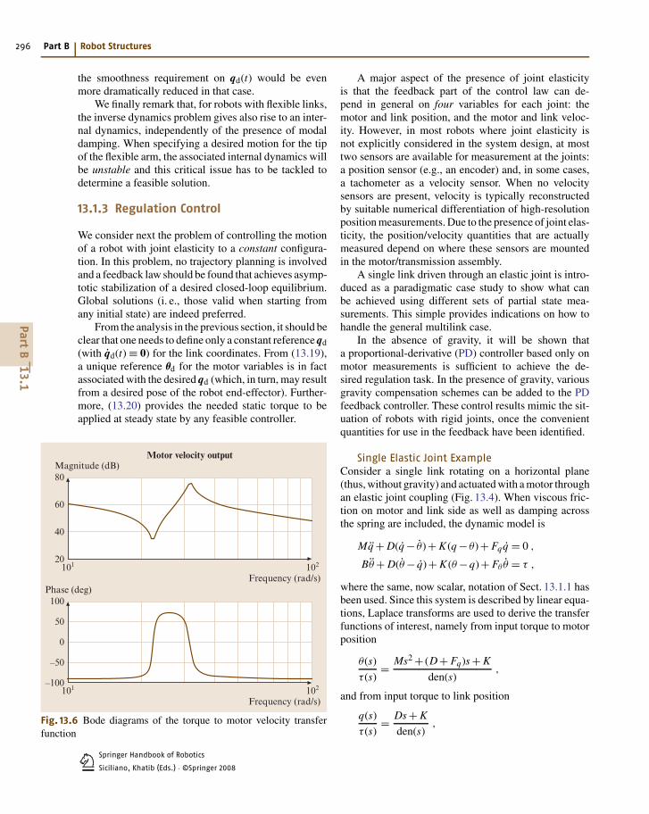
Fig. 13.6 Bode diagrams of the torque to motor velocity transferfunction
A major aspect of the presence of joint elasticityis that the feedback part of the control law can de-pend in general on four variables for each joint: themotor and link position, and the motor and link veloc-ity. However, in most robots where joint elasticity isnot explicitly considered in the system design, at mosttwo sensors are available for measurement at the joints:a position sensor (e.g., an encoder) and, in some cases,a tachometer as a velocity sensor. When no velocitysensors are present, velocity is typically reconstructedby suitable numerical differentiation of high-resolutionposition measurements. Due to the presence of joint elas-ticity, the position/velocity quantities that are actuallymeasured depend on where these sensors are mountedin the motor/transmission assembly.
A single link driven through an elastic joint is intro-duced as a paradigmatic case study to show what canbe achieved using different sets of partial state mea-surements. This simple provides indications on how tohandle the general multilink case.
In the absence of gravity, it will be shown thata proportional-derivative (PD) controller based only onmotor measurements is sufficient to achieve the de-sired regulation task. In the presence of gravity, variousgravity compensation schemes can be added to the PDfeedback controller. These control results mimic the sit-uation of robots with rigid joints, once the convenientquantities for use in the feedback have been identified.
Single Elastic Joint ExampleConsider a single link rotating on a horizontal plane(thus, without gravity) and actuated with a motor throughan elastic joint coupling (Fig. 13.4). When viscous fric-tion on motor and link side as well as damping acrossthe spring are included, the dynamic model is
Mq + D(q − θ)+ K (q − θ)+ Fqq = 0 ,
Bθ + D(θ − q)+ K (θ −q)+ Fθ θ = τ ,
where the same, now scalar, notation of Sect. 13.1.1 hasbeen used. Since this system is described by linear equa-tions, Laplace transforms are used to derive the transferfunctions of interest, namely from input torque to motorposition
θ(s)
τ(s)= Ms2 + (D + Fq)s + K
den(s),
and from input torque to link position
q(s)
τ(s)= Ds + K
den(s),
PartB
13.1
Springer Handbook of Robotics
Siciliano, Khatib (Eds.) · ©Springer 2008 1
Robots with Flexible Elements 13.1 Robots with Flexible Joints 297
with the common denominator den(s) given by
den(s) ={
MB s3 + [M(D + Fθ )+ B(D + Fq)
]s2
+ [(M + B)K + (Fq + Fθ )D + Fq Fθ
]s
+(Fq + Fθ )K}
s .
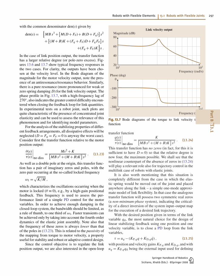
In the case of link position output, the transfer functionhas a larger relative degree (or pole-zero excess). Fig-ures 13.6 and 13.7 show typical frequency responses inthe two cases. For clarity, the outputs have been cho-sen at the velocity level. In the Bode diagram of themagnitude for the motor velocity output, note the pres-ence of an antiresonance/resonance behavior. Similarly,there is a pure resonance (more pronounced for weak orzero spring damping D) for the link velocity output. Thephase profile in Fig. 13.7, with a high-frequency lag of270◦, also indicates the greater control difficulty encoun-tered when closing the feedback loop for link quantities.In experimental tests on a robot joint, such plots arequite characteristic of the presence of concentrated jointelasticity and can be used to assess the relevance of thisphenomenon and for identifying model parameters.
For the analysis of the stabilizing properties of differ-ent feedback arrangements, all dissipative effects will beneglected (D = Fq = Fθ = 0 is anyway the worst case).Consider first the transfer function relative to the motorposition output:
θ(s)
τ(s)
∣∣∣∣no diss
= Ms2 + K[MB s2 + (M + B)K
]s2
. (13.23)
As well as a double pole at the origin, this transfer func-tion has a pair of imaginary zeros and poles, with thezero pair occurring at the so-called locked frequency
ω1 = √K/M ,
which characterizes the oscillations occurring when themotor is locked (θ ≡ 0), e.g., by a high-gain positionalfeedback. This frequency is used to assess the per-formance limit of a simple PD control for the motorvariables. In order to achieve enough damping in theclosed-loop system, the bandwidth should be limited, asa rule of thumb, to one third of ω1. Faster transients canbe achieved only by taking into account the fourth-orderdynamics of the elastic joint assembly. Note also thatthe frequency of these zeros is always lower than thatof the poles in (13.23). This is related to the passivity ofthe mapping from torque to motor velocity, a propertyuseful for stability and robust or adaptive control design.
Since the control objective is to regulate the linkposition output, we are also interested in the open-loop
101 102
Link velocity output
Phase (deg)
Frequency (rad/s)
0
–100
–200
–300
101 102
Magnitude (dB)
Frequency (rad/s)
80
60
40
20
Fig. 13.7 Bode diagrams of the torque to link velocity transferfunction
transfer functionq(s)
τ(s)
∣∣∣∣no diss
= K[MB s2 + (M + B)K
]s2
. (13.24)
This transfer function has no zeros (in fact, for this it issufficient to have D = 0) so that the relative degree isnow four, the maximum possible. We shall see that thenonlinear counterpart of the absence of zeros in (13.24)will play a relevant role also for trajectory control in themultilink case of robots with elastic joints.
It is also worth mentioning that this situation iscompletely different from the case in which the elas-tic spring would be moved out of the joint and placedanywhere along the link – a simple one-mode approxi-mate model of link flexibility. In that case the analogoustransfer function will possess two symmetric real zeros(a non-minimum-phase system), indicating the critical-ity of a direct inversion of the system input–output mapfor the execution of a desired link trajectory.
With the desired position given in terms of the linkvariable qd, the most natural choice for the design oflinear stabilizing feedback using one position and onevelocity variable, is to close a PD loop from the linkvariables,
τ = uq − (KP,qq + KD,qq) , (13.25)
with position and velocity gains KP,q and KD,q , and withuq = KP,qqd being the external input used for defining
PartB
13.1
Springer Handbook of Robotics
Siciliano, Khatib (Eds.) · ©Springer 20081
298 Part B Robot Structures
the set point. It is easy to verify that the closed-loop poleswill be unstable no matter how the gains are chosen, sothat error feedback from link variables alone should beavoided. In a similar way, also the combination of motorposition and link velocity feedback is always unstable.
Another mixed feedback strategy is to use link posi-tion and motor velocity:
τ = uq − (KP,qq + KD,mθ) . (13.26)
This combination corresponds, e.g., to the case ofa tachometer integrated in a direct-current (DC) mo-tor and of an optical encoder placed on the load shaft forsensing its position (without any knowledge about therelevance of joint elasticity). Use of (13.26) leads to theclosed-loop characteristic equation
BMs4 + MKD,ms3 + (B + M)Ks2
+KKD,ms + KKP,q = 0 .
Using Routh’s criterion, asymptotic stability occurs ifand only if the motor velocity gain KD,m > 0 and the linkposition gain satisfies 0 < KP,q < K , i. e., the propor-tional feedback should not override the spring stiffness.The existence of such an upper bound limits the useful-ness of this scheme.
Finally, performing feedback from the motor vari-ables
τ = uθ − (KP,mθ + KD,mθ) , (13.27)
the closed-loop system will be asymptotically stableprovided that both KP,m and KD,m are strictly positive(and otherwise arbitrarily large). This favorable situa-tion lends itself to a convenient generalization in themultilink case.
Note that other partial state feedback combinationswould be possible, depending on the available sensingdevices. For instance, mounting a strain gauge on thetransmission shaft provides a direct measure of the elas-tic torque τJ = K (θ −q) for control use. Strain gaugesare also useful sensors for flexible links. Indeed, full-state feedback may be designed so as to guaranteeasymptotic stability and improve the transient behav-ior considerably; however, this would be obtained at thecost of additional sensors and requires proper tuning ofthe four gains.
PD Control Using only Motor VariablesFor the general multilink case in the absence of gravity,consider the PD control law based on motor position andvelocity feedback
τ = K P(θd − θ)− K Dθ , (13.28)
with symmetric (typically, diagonal) positive-definitegain matrices K P and K D. Since g(q) ≡ 0, it followsfrom (13.19) that the reference value for the motor posi-tion is θd = qd (no joint deflection is present nor an inputtorque is needed at steady state).
The control law (13.28) globally asymptoticallystabilizes the desired equilibrium state q = θ = qd,q = θ = 0. This can be shown through a Lyapunovargument, completed by the application of La Salle’stheorem. In fact, a candidate Lyapunov function is givenby the sum of the total energy of the system (kineticplus elastic potential) and of the control energy due tothe proportional term (a virtual elastic potential energy):
V =1
2Θ�M(Θ)Θ+ 1
2(q − θ)�K (q − θ)
+ 1
2(θd − θ)�K P(θd − θ) ≥ 0 . (13.29)
Computing the time derivative of V along the trajectoriesof the closed-loop system given by (13.7) (or (13.9))and (13.28), and taking into account the skew-symmetryof M −2C, leads to
V = −θ�K Dθ ≤ 0 .
The inclusion of dissipative terms (viscous friction andspring damping) would render V even more negative-semidefinite. The analysis is completed by verifying thatthe maximum invariant set contained in the set of statessuch that V = 0 (i. e., those with θ = 0) collapses intothe desired unique equilibrium state.
We point out that an identical control law is able toglobally regulate, in the absence of gravity, robots withflexible links to a desired joint configuration. In thatcase, θ in (13.28) would be the rigid coordinates at thebase of the flexible links of the robot.
PD with Constant Gravity CompensationThe presence of gravity requires the addition of someform of gravity compensation to the PD action (13.28).Moreover, this will need an additional structural assump-tion and may demand some caution in the selection ofthe control gains.
Before proceeding, we recall a basic property of thegravity vector g(q) (under assumption A2, the gravityvector in (13.7) is the same as that appearing in thedynamics of the equivalent rigid robot): for robots withrotational joints, elastic or not, a positive constant α
exists such that∥∥∥∥∂g(q)
∂q
∥∥∥∥ ≤ α, ∀q ∈ RN . (13.30)
PartB
13.1
Springer Handbook of Robotics
Siciliano, Khatib (Eds.) · ©Springer 2008 1
Robots with Flexible Elements 13.1 Robots with Flexible Joints 299
The norm of a matrix A(q) is that induced by the Eu-
clidean norm for vectors, i. e., ‖A‖ =√
λmax(
A� A).
Inequality (13.30) implies that
‖g(q1)− g(q2)‖ ≤ α‖q1 −q2‖, ∀q1, q2 ∈ RN .
(13.31)
In common practice, robot joints are never unrealis-tically soft. More precisely, they are stiff enough to have,under the load of the robot’s own weight, a unique equi-librium link position qe associated with any assignedfixed motor position θe – the reverse of the relation-ship expressed by (13.19). This situation is by no meansrestrictive, but will be stated for clarity as a furthermodeling assumption:
A5 The lowest joint stiffness is larger than the upperbound on gravity forces acting on the robot, or
mini=1,...N Ki > α .
The simplest modification for handling the presenceof gravity is to consider the addition of a constant termthat compensates exactly the gravity load at the de-sired steady state. According to (13.19) and (13.20),the control law (13.28) is then modified to
τ = K P(θd − θ)− K Dθ + g(qd) , (13.32)
with symmetric, typically diagonal, K P > 0 (as a mini-mum) and K D > 0, and with the motor reference givenby θd = qd + K−1g(qd).
A sufficient condition guaranteeing that q = qd,θ = θd, q = θ = 0 will be a globally asymptotically sta-ble equilibrium for the system (13.7) under the controllaw (13.32) is that
λmin
[(K −K
−K K + K P
)]> α , (13.33)
with α defined in (13.30). Taking into account the diag-onal structure of K and K P , and thanks to assumptionA5, it is always possible to fulfill this condition by in-creasing the smallest proportional gain in the controller(or, the smallest eigenvalue of K P if this matrix has notbeen chosen diagonal).
In the following, we sketch the motivation for thiscondition and the associated proof of asymptotic stabil-ity. The equilibrium positions of the closed-loop systemare the solutions of
K (q − θ)+ g(q) = 0 ,
K (θ −q)− K P(θd − θ)− g(qd) = 0 .
Indeed, the pair (qd, θd) satisfies these equations. How-ever, in order to obtain a global result one should
guarantee that this pair is the unique solution. There-fore, recalling (13.19), the null term K (θd −qd)− g(qd)can be added/subtracted to both equations to obtain
K (q −qd)− K (θ − θd) = g(qd)− g(q)
−K (q −qd)+ (K + K P)(θ − θd) = 0 ,
where the matrix in condition (13.33) can be clearlyrecognized. Taking the norms of terms on both sidesand bounding gravity terms using (13.31), the introducedcondition (13.33) implies that the pair (qd, θd) is in factthe unique equilibrium. To show asymptotic stability,a candidate Lyapunov function is built based on thatused in the absence of gravity (13.29):
Vg1 = V +Ugrav(q)−Ugrav(qd)− (q −qd)�g(qd)
− 1
2g�(qd)K−1g(qd) ≥ 0 . (13.34)
The last constant term is used to set the minimumvalue of Vg1 to zero at the desired equilibrium. Thepositive-definiteness of Vg1 and the fact that its uniqueminimum is at the desired state are again implied by con-dition (13.33). By the usual computations, it follows thatVg1 = −θ�K Dθ ≤ 0 and the result is obtained applyingLa Salle’s theorem.
The control law (13.32) is based only on the know-ledge of the gravity term g(qd) and of the joint stiffnessK . The latter appears in fact in the definition of the motorposition reference θd. Uncertainties in the gravitationalterm g(qd) and on the joint stiffness K affect the perfor-mance of the controller. Still, the existence of a uniqueclosed-loop equilibrium and its asymptotic stability arepreserved when the gravity bound by α is still correctand condition (13.33) holds for the true stiffness values.Indeed, the robot will converge to an equilibrium that isdifferent from the desired one – the better the estimatesK and g(qd) used, the closer the actual equilibrium willbe to the desired one.
PD with Online Gravity CompensationSimilarly to the rigid robot case, a better transient be-havior is to be expected if gravity compensation (or,more precisely, its perfect cancellation) is performed atall configurations during motion. However, the gravityvector in (13.7) depends on the link variables q, whichare assumed not to be measurable at this stage. It is easyto see that using g(θ), with the measured motor posi-tions in place of the link positions, leads in general toan incorrect closed-loop equilibrium. Moreover, evenif q were available, adding g(q) to a motor PD errorfeedback has no guarantee of success because this com-pensation, which appears in the motor equation, does
PartB
13.1
Springer Handbook of Robotics
Siciliano, Khatib (Eds.) · ©Springer 20081
300 Part B Robot Structures
not instantaneously cancel the gravity load acting on thelinks.
With this in mind, a PD control with online gravitycompensation can be introduced as follows. Define thevariable
θ = θ − K−1g(qd) , (13.35)
which is a gravity-biased modification of the measuredmotor position θ, and let
τ = K P (θd − θ)− K Dθ + g(θ) , (13.36)
where K P > 0 and K D > 0 are both symmetric (andtypically diagonal) matrices. The control law (13.36)can still be implemented using only motor variables. Theterm g(θ) only provides an approximate cancellation(though of a large part) of gravity during motion, butleads to the correct gravity compensation in the steadystate. In fact, by using (13.19) and (13.35), it followsthat
θd := θd − K−1g(qd) = qd ,
so that g(θd) = g(qd).Global asymptotic stability of the desired equilib-
rium can be guaranteed under the same condition (13.33)used for the constant gravity compensation case.A slightly different Lyapunov candidate is defined, start-ing again from the one in (13.29), as
Vg2 = V +Ugrav(q)−Ugrav(θ)
−1
2g�(qd)K−1g(qd) ≥ 0 ,
to be compared with (13.34).The use of an online gravity compensation scheme
typically provides a smoother time course and a notice-able reduction of the positional transient errors, withno additional control effort in terms of peak and averagetorques. We note that choices of low position gains, evenwhen largely violating the sufficient condition (13.33)for stability, may still work, contrary to the case of con-stant gravity compensation. However also for increasingvalues of joint stiffness, in the limit for K → ∞, therange of feasible values of K P that guarantee exactregulation does not extend down to zero.
A possibility to refine the online gravity compen-sation scheme, again based only on motor positionmeasurement, is offered by the use of a fast iterativealgorithm that elaborates the measure θ in order togenerate a quasistatic estimate q(θ) of the current (un-measured) q. In fact, in any steady-state configuration(qs, θs), a direct mapping is defined from qs to θs:
θs = hg(qs) := qs + K−1g(qs) .
Assumption A5 is sufficient to guarantee the exis-tence and uniqueness also of the inverse mappingqs = h−1
g (θs). For a measured θ, the function
q = T(q) := θ − K−1g(q)
is then a contraction mapping and the iteration
qi+1 = T(qi ), i = 0, 1, 2, . . .
will converge to the unique fixed point of this mapping,which is exactly the value q(θ) = h−1
g (θ). A suitable ini-tialization for q0 is either the measured θ or the value qcomputed at the previous sampling instant. In this way,just two or three iterations are needed to obtain suffi-cient accuracy and this is fast enough to be implementedwithin a sensing/control sampling interval of a digitalrobot controller.
With this iterative scheme running in the back-ground, the regulation control law becomes
τ = K P (θd − θ)− K Dθ + g[q(θ)
], (13.37)
with symmetric (diagonal) K P > 0 and K D > 0. A proofof the global asymptotic stability of this control schemecan be given by further modifying the previous Lya-punov candidates. The advantage of (13.37) is that anypositive value of the feedback gain K P is allowed, thusrecovering in full the operative working conditions ofthe rigid case with exact gravity cancellation.
Both online gravity compensation schemes (13.36)and (13.37) realize a compliance control in the jointspace with only motor measurements. The same ideacan also be extended to the case of Cartesian compliancecontrol by evaluating the direct kinematics and the Jaco-bian (transpose) of the robot arm with θ or, respectively,q(θ) in place of q.
Full-State FeedbackWhen the feedback law is based on a full set of meas-urements of the robot state, the transient performanceof regulation control laws can be improved. Taking ad-vantage of the availability of a joint torque sensor, wepresent a convenient design for the reduced model (13.9)of robots with elastic joints, including spring dampingas a dissipation effect. Full-state feedback can be ob-tained in two phases, by combining a preliminary torquefeedback with the motor feedback law in (13.28).
Using τJ = K (θ −q), the motor equation can berewritten as
Bθ +τJ + DK−1τJ = τ .
PartB
13.1
Springer Handbook of Robotics
Siciliano, Khatib (Eds.) · ©Springer 2008 1
Robots with Flexible Elements 13.1 Robots with Flexible Joints 301
The joint torque feedback
τ = BB−1θ u+ (
I − BB−1θ
)(τJ + DK−1τJ
), (13.38)
where u is an auxiliary input to be designed, transformsthe motor equations into
Bθ θ +τJ + DK−1τJ = u .
In this way, the apparent motor inertia can be reduced toa desired, arbitrary small value Bθ , with clear benefitsin terms of vibration damping. For instance in the linearand scalar case, a very small B shifts the pair of complexpoles in (13.23) to a very high frequency, with the jointbehaving almost as a rigid one.
Setting
u = K P,θ (θd − θ)− K D,θ θ + g(qd)
in (13.38) leads to the state feedback controller
τ = K P(θd − θ)− K Dθ + KT [g(qd)−τJ]− KSτJ + g(qd) , (13.39)
with gains
K P = BB−1θ K P,θ ,
K D = BB−1θ K D,θ ,
KT = BB−1θ − I
and
KS =(
BB−1θ − I
)DK−1 .
Indeed, the law (13.39) can also be rewritten in terms of(θ, q, θ, q), if the torque sensor is not available. How-ever, keeping this structure of the gains preserves theinteresting physical interpretation of what the full-statefeedback controller is achieving.
13.1.4 Trajectory Tracking
As for rigid robot arms, the problem of tracking desiredtime-varying trajectories is harder for robots with elas-tic joints than achieving constant regulation. In general,solving this problem requires the use of full-state feed-back and knowledge of all the terms in the dynamicmodel.
Under these conditions, we shall focus on the feed-back linearization approach, namely a a nonlinear statefeedback law that leads to a closed-loop system with de-coupled and exactly linear behavior for all the N degreesof freedom of the robot (in fact, the link variables q). Thetracking errors along the reference trajectory are forcedto be globally exponentially stable, with a decaying ratethat can be directly specified through the choice of the
scalar feedback gains in the controller. This fundamentalresult is the direct extension of the well-known computedtorque method for rigid robots. Because of its relevantproperties, the feedback linearization approach can beused as a reference to assess the performance of anyother trajectory tracking control law, which may possiblybe designed using less/approximate model informationand/or only partial-state feedback.
However, in the presence of joint elasticity, thedesign of a feedback linearization law is not straight-forward. Furthermore, as soon as S �= 0, the dynamicmodel (13.7) will not satisfy the existing necessary con-ditions for exact linearization (nor those for input–outputdecoupling) when only a static (or, instantaneous) feed-back law from the full state is allowed. Therefore, wewill restrict our attention to the more tractable case of thereduced dynamic model (13.9) and sketch only brieflythe more general picture.
As a second much simpler approach to trajectorytracking problems, we also present a linear controldesign that makes use of a model-based feedforwardcommand and a precomputed state reference trajectory,as obtained from the inverse dynamics computationsof Sect. 13.1.2, with the addition of a linear feedbackfrom the full state. In this case, convergence to thedesired trajectory is only locally guaranteed, i. e., thetracking errors should be small enough, but the con-trol implementation is straightforward and the real-timecomputational burden is considerably reduced.
Feedback LinearizationConsider the reduced model (13.9) and let the refer-ence trajectory be specified by a desired smooth linkmotion qd(t). The control design will proceed by sys-tem inversion, in a similar way to the inverse dynamicscomputations of Sect. 13.1.2 but using now the currentmeasures of the state variables (q, θ, q, θ) instead ofthe reference state evolution (qd, θd, qd, θd). Notably,there is no need to transform the robot equations intotheir state-space description, which is the standard formused in control design for general nonlinear systems;we will use the robot model directly in its second-orderdifferential form (typical of mechanical systems).
The outcome of the inversion procedure will be thedefinition of a torque τ, in the form of a static statefeedback control law, which cancels the original robotdynamics and replaces it with a desired linear and de-coupled one of suitable differential order. In this sense,the control law stiffens the dynamics of the robot withelastic joints. The feasibility of inverting the system fromthe chosen output q without causing instability prob-
PartB
13.1
Springer Handbook of Robotics
Siciliano, Khatib (Eds.) · ©Springer 20081
302 Part B Robot Structures
lems (related to the presence of unobservable dynamicsin the closed-loop system, after cancellation) is a rele-vant property of robots with elastic joints. In fact, this isthe direct generalization to the nonlinear multiple-inputmultiple-output (MIMO) case of the possibility of in-verting a scalar transfer function in the absence of zeros(see also the considerations made on (13.24)).
Rewrite the link equation in the compact form
M(q)q +n(q, q)+ K (q − θ) = 0 , (13.40)
where again we set n(q, q) = c(q, q)+ g(q). None of theabove quantities depends instantaneously on the inputtorque τ. Therefore, we can differentiate once and obtain
M(q)q[3] + M(q)q + n(q, q)+ K (q − θ) = 0 .
(13.41)
Proceeding one step further leads to
M(q)q[4] +2M(q)q[3] + M(q)q
+n(q, q)+ K (q − θ) = 0 , (13.42)
where θ now appears. The motor acceleration is at thesame differential level of τ in the motor equation
Bθ + K (θ −q) = τ , (13.43)
and thus, replacing θ from (13.43), we get
M(q)q[4] +2M(q)q[3] + M(q)q + n(q, q)+ Kq
= K B−1 [τ − K (θ −q)] . (13.44)
We note that, using (13.40), the last term K (θ −q)in (13.44) may also be replaced by M(q)q +n(q, q).
Since the matrix A(q) = M−1(q)K B−1 is alwaysnonsingular, an arbitrary value v can be assigned to thefourth derivative of q by a suitable choice of the inputtorque τ. The matrix A(q) is the so-called decouplingmatrix of the system and its nonsingularity is a neces-sary and sufficient condition for imposing a decoupledinput-output behavior by nonlinear static state feedback.Moreover, (13.44) indicates that each component qi of qneeds to be differentiated ri = 4 times in order to be al-gebraically related to the input torque τ (ri is the relativedegree of qi , when this is chosen as a system output).Since there are N link variables, the total sum of the rela-tive degrees is 4N , equal to the dimension of the state ofa robot with elastic joints. All these facts taken togetherlead to the conclusion that, when inverting (13.44) to de-termine the input τ that imposes q[4] = v, there will beno other dynamics left other than the one appearing inthe closed-loop input–output map.
Therefore, choose
τ = BK−1[
M(q)v+α(q, q, q, q[3])]
+ [M(q)+ B
]q +n(q, q) , (13.45)
with
α(q, q, q, q[3]) = M(q)q +2M(q)q[3] + n(q, q) ,
where the terms in α have been ordered according to thedependence on increasing orders of derivatives of q. Thecontrol law (13.45) leads to a closed-loop system fullydescribed by
q[4] = v , (13.46)
i. e., chains of four input–output integrators from eachauxiliary input vi to each link position output qi , fori = 1, . . . , N . The robot system thus has been exactlylinearized and decoupled by the nonlinear feedbacklaw (13.45).
The complete control law (13.45) is expressedas a function of the so-called linearizing coordinates(q, q, q, q[3]) only. This has led to some misunder-standings in the past, as it seemed that the feedbacklinearization approach for robots with elastic jointswould need direct measures of the link acceleration q andjerk q[3], which are impossible to obtain with currentlyavailable sensors (or would require multiple numericaldifferentiations of position measures in real time, withcritical noise problems).
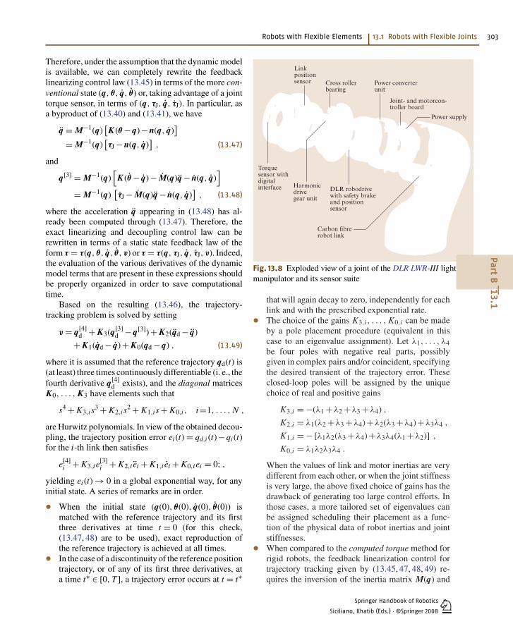
When considering the latest technology in the field,it is now feasible to have a set of sensors for elasticjoints measuring in a reliable and accurate way the motorposition θ (and, possibly, also its velocity θ), the jointtorque τJ = K (θ −q), as well as the link position q. Forinstance, this is the arrangement of sensors availableat each joint of the LWR-III lightweight manipulator,where Hall sensors are used for the motor position, jointtorque sensing is based on strain gauges, and a high-endcapacitive sensor is used for the link position (Fig. 13.8).Therefore, only one numerical differentiation is neededin order to obtain a good estimate of q and/or τJ as well.Note that, depending on the specific sensor resolution, itmay also be convenient to evaluate q using the measuresof θ and τ J as θ − K−1τJ.
With this in mind, it is easy to see that the followingthree sets of 4N variables
(q, q, q, q[3]) , (q, θ, q, θ) , (q, τJ, q, τJ)
are all equivalent state variables for a robot with elas-tic joints, related by globally invertible transformations.
PartB
13.1
Springer Handbook of Robotics
Siciliano, Khatib (Eds.) · ©Springer 2008 1
Robots with Flexible Elements 13.1 Robots with Flexible Joints 303
Therefore, under the assumption that the dynamic modelis available, we can completely rewrite the feedbacklinearizing control law (13.45) in terms of the more con-ventional state (q, θ, q, θ) or, taking advantage of a jointtorque sensor, in terms of (q, τJ, q, τJ). In particular, asa byproduct of (13.40) and (13.41), we have
q = M−1(q)[K (θ −q)−n(q, q)
]= M−1(q)
[τJ −n(q, q)
], (13.47)
and
q[3] = M−1(q)[
K (θ − q)− M(q)q − n(q, q)]
= M−1(q)[τJ − M(q)q − n(q, q)
], (13.48)
where the acceleration q appearing in (13.48) has al-ready been computed through (13.47). Therefore, theexact linearizing and decoupling control law can berewritten in terms of a static state feedback law of theform τ = τ(q, θ, q, θ, v) or τ = τ(q, τJ, q, τJ, v). Indeed,the evaluation of the various derivatives of the dynamicmodel terms that are present in these expressions shouldbe properly organized in order to save computationaltime.
Based on the resulting (13.46), the trajectory-tracking problem is solved by setting
v = q[4]d + K3(q[3]
d −q[3])+ K2(qd − q)
+ K1(qd − q)+ K0(qd −q) , (13.49)
where it is assumed that the reference trajectory qd(t) is(at least) three times continuously differentiable (i. e., thefourth derivative q[4]
d exists), and the diagonal matricesK0, . . . , K3 have elements such that
s4 + K3,i s3 + K2,i s
2 + K1,i s + K0,i , i=1, . . . , N ,
are Hurwitz polynomials. In view of the obtained decou-pling, the trajectory position error ei (t) = qd,i (t)−qi (t)for the i-th link then satisfies
e[4]i + K3,i e
[3]i + K2,i ei + K1,i ei + K0,i ei = 0; ,
yielding ei (t) → 0 in a global exponential way, for anyinitial state. A series of remarks are in order.
• When the initial state (q(0), θ(0), q(0), θ(0)) ismatched with the reference trajectory and its firstthree derivatives at time t = 0 (for this check,(13.47, 48) are to be used), exact reproduction ofthe reference trajectory is achieved at all times.• In the case of a discontinuity of the reference positiontrajectory, or of any of its first three derivatives, ata time t∗ ∈ [0, T ], a trajectory error occurs at t = t∗
Linkposition sensor
Torquesensor withdigitalinterface Harmonic
drive gear unit
DLR robodrive with safety brakeand positionsensor
Carbon fibrerobot link
Cross rollerbearing
Power converterunit
Joint- and motorcon-troller board
Power supply
Fig. 13.8 Exploded view of a joint of the DLR LWR-III lightweightmanipulator and its sensor suite
that will again decay to zero, independently for eachlink and with the prescribed exponential rate.• The choice of the gains K3,i , . . . , K0,i can be madeby a pole placement procedure (equivalent in thiscase to an eigenvalue assignment). Let λ1, . . . , λ4be four poles with negative real parts, possiblygiven in complex pairs and/or coincident, specifyingthe desired transient of the trajectory error. Theseclosed-loop poles will be assigned by the uniquechoice of real and positive gains
K3,i = −(λ1 +λ2 +λ3 +λ4) ,
K2,i = λ1(λ2 +λ3 +λ4)+λ2(λ3 +λ4)+λ3λ4 ,
K1,i = − [λ1λ2(λ3 +λ4)+λ3λ4(λ1 +λ2)] ,
K0,i = λ1λ2λ3λ4 .
When the values of link and motor inertias are verydifferent from each other, or when the joint stiffnessis very large, the above fixed choice of gains has thedrawback of generating too large control efforts. Inthose cases, a more tailored set of eigenvalues canbe assigned scheduling their placement as a func-tion of the physical data of robot inertias and jointstiffnesses.• When compared to the computed torque method forrigid robots, the feedback linearization control fortrajectory tracking given by (13.45, 47, 48, 49) re-quires the inversion of the inertia matrix M(q) and
PartB
13.1
Springer Handbook of Robotics
Siciliano, Khatib (Eds.) · ©Springer 20081
304 Part B Robot Structures
the additional evaluation of derivatives of the inertiamatrix and of other terms in the dynamic model.• The feedback linearization approach can also beapplied without any changes in the presence of vis-cous (or otherwise smooth) friction at the motor andlink side. The inclusion of spring damping leads in-stead to a third-order decoupled differential relationbetween the auxiliary input v and q, leaving thus a N-dimensional unobservable but asymptotically stabledynamics in the closed-loop system. In this case,only input–output (and not full-state) linearizationand decoupling is achieved.
We conclude with some considerations on exactlinearization/decoupling for the general model (13.7)of robots with elastic joints. Unfortunately, due to thepresence of the inertial coupling matrix S(q) betweenlinks and rotors, the above control design can no longerbe applied. Consider as an illustration the case ofa constant S in (13.7), with the associated model sim-plifications. Solving for θ from the motor equations,θ = B−1
(τ −τJ − S�q
), and substituting into the link
equations leads to[M(q)− SB−1S�]
q +n(q, q)−(
I + SB−1)
τJ
= −SB−1τ .
In this case, the input torque τ appears already in theexpression for the link acceleration q. Using (13.6), theexpression of the decoupling matrix is then
A(q) = − [ML(q)+ MR(q)]−1 SB−1 ,
which is never full rank in view of the structure (13.5) ofS. As a consequence, the necessary condition for obtain-ing (at least) input–output linearization and decouplingby static state feedback fails to hold.
However, by resorting to the use of a larger classof control laws, it is still possible to obtain an exactlinearization and decoupling result. For this purpose,consider a dynamic state feedback controller of the form
τ = α(q, q, θ, θ, ξ)+β(q, q, θ, θ, ξ)v ,
ξ = γ (q, q, θ, θ, ξ)+ δ(q, q, θ, θ, ξ)v , (13.50)
where ξ ∈ Rν is the state of the dynamic compensator,
α, β, γ , and δ are suitable nonlinear vector functions,and v ∈ R
N is (as before) an external input used fortrajectory-tracking purposes. It is possible to show ingeneral that a dynamic compensator (13.50) of orderat most ν = 2N(N −1) can be designed so as to yield
a closed-loop system that is globally described by
q[2(N+1)] = v ,
in place of (13.46). Note the coincidence of this differ-ential order with the one found for exact reproducibilityof a desired trajectory qd(t) in Sect. 13.1.2. The trackingproblem is then solved by a direct generalization of thelinear stabilization design of (13.49).
It is interesting to give a physical interpretation forthis control result. The structural obstruction to input–output decoupling of the model (13.7) is that the motionof a link attached to an elastic joint is affected too soon(at the second differential level) by torques originating atother elastic joints. This is due to the inertial couplingspresent between the motors and links. The addition ofdynamics (i. e., of integrators) in the controller slowsdown these low-energy paths and allows for the high-energy effects of the elastic torque at the local joint(a fourth-order differential path) to come into play. Thisdynamic balancing allows both input–output decouplingand exact linearization of the extended system (havingthe robot and the controller states).
Linear Control DesignThe feedback linearization approach to trajectory track-ing gives rise to a rather complex nonlinear control law.Its main advantage of globally enforcing a linear and de-coupled behavior on the trajectory error dynamics can betraded off with a control design that achieves only localstability around the reference trajectory, but is muchsimpler to implement (and may run at higher samplingrates).
For this, the inverse dynamics results of Sect. 13.1.2can be used, assuming either the reduced or the completerobot model and with or without dissipative terms. Givena sufficiently smooth desired link trajectory qd(t), wehave seen that it is always possible to associate:
1. the nominal torque τd(t) needed for its exact repro-duction, and
2. the reference evolution of all other state variables(e.g., θd(t), as given by (13.13), or τJ,d(t)).
These signals define a sort of steady-state operationfor the system.
A simpler tracking controller combines a model-based feedforward term with a linear feedback termusing the trajectory error: the linear feedback locallystabilizes the system around the reference state trajec-tory, whereas the feedforward torque is responsible formaintaining the robot along the desired motion when theerror has vanished.
PartB
13.1
Springer Handbook of Robotics
Siciliano, Khatib (Eds.) · ©Springer 2008 1
Robots with Flexible Elements 13.1 Robots with Flexible Joints 305
Using full-state feedback, two possible controllersof this kind are
τ = τd + K P,θ (θd − θ)+ K D,θ (θd − θ)
+ K P,q(qd −q)+ K D,q(qd − q) (13.51)
and
τ = τd + K P,θ (θd − θ)+ K D,θ (θd − θ)
+ K P,J (τJ,d −τJ)+ K D,J (τJ,d − τJ) . (13.52)
These trajectory tracking schemes are the most commonin the control practice for robots with elastic joints. Inthe absence of full-state measurements, they can be com-bined with an observer of the unmeasurable quantities.An even simpler realization is
τ = τd + K P(θd − θ)+ K D(θd − θ) , (13.53)
which uses only motor measurements and relies on theresults obtained for the regulation case.
The different gain matrices used in (13.51, 52, 53)have to be tuned using a linear approximation of therobot system. This approximation may be obtained ata fixed equilibrium point or around the actual referencetrajectory, leading respectively to a linear time-invariantor to a linear time-varying system. While the existenceof (possibly time-varying) stabilizing feedback matricesis guaranteed by the controllability of these linear ap-proximations, the validity of the approach is only localin nature and the region of convergence will dependboth on the given trajectory and on the robustness of thedesigned linear feedback.
It should be mentioned that such a control approachto trajectory tracking problems can also be used forrobots with flexible links. Once the inverse dynamicsproblem has been solved (for the case of link flexibility,this typically results in a noncausal solution), a controllerof the form (13.53) (or (13.51), with link deflection δ anddeflection rate δ replacing, respectively, q and q), can bedirectly applied.
13.1.5 Further Reading
This section contains the main references for the part ofthis chapter on robots with joint flexibility. In addition,we indicate to a larger bibliography for topics that havenot been included here.
Early interest in problems arising from the presenceof flexible transmissions in robot manipulators datesback to [13.1, 2], with first experimental findings on theGE P-50 arm. Relevant mechanical considerations in-volved in the design of robot arms and in the evaluationof their compliant elements can be found in [13.3].
One of the first studies on the inclusion of joint elas-ticity in the dynamic modeling of robot arms is dueto [13.4]. The detailed analysis of the model structurepresented in Sect. 13.1.1 comes from [13.5], with someupdates from [13.6]. The simplifying assumption lead-ing to the reduced model was introduced in [13.7]. Thespecial case of motors mounted on the driven links isconsidered in [13.8]. The observation that joints withlimited elasticity lead to a singularly perturbed dynamicmodel was first recognized in [13.9]. Symbolic manipu-lation programs for the automatic generation of dynamicmodels of robots with elastic joints were also developedvery early [13.10].
The inverse dynamics computations in Sect. 13.1.2can be traced back to [13.11]. The use of programssuch as Modelica for the numerical evaluation of inversedynamics is highlighted in [13.6].
The first specific control designs were basedon decentralized linear controllers, see, e.g., [13.12]and [13.13], where a fourth-order dynamics local to eachelastic joint was used. However, schemes with provedglobal convergence characteristics appeared only later.
In Sect. 13.1.3, the PD controller with constant grav-ity compensation is a contribution of [13.14]. Thiswas also extended to the case of robots with flexiblelinks in [13.15]. The two versions of regulation controlwith online gravity compensation are due, respectively,to [13.16] and [13.17]. Both these control laws wereextended to Cartesian compliance schemes in [13.18]and [13.19]. A general regulation framework based onenergy shaping has been proposed in [13.20]. In the ab-sence of any information on gravity, a PID regulatorwith semiglobal stability properties has been presentedin [13.21], while a global learning scheme was proposedin [13.22].
The presentation of a full-state feedback designfor regulation (and tracking) follows the idea usedin [13.23]. Special interest has been devoted over theyears to joint torque feedback, from the placement oftorque sensors on transmission shafts [13.24] or withinharmonic drives [13.25] to their use for achieving robustcontrol performance [13.26].
The fact that the reduced model of robots with elas-tic joints can always be feedback linearized via staticstate feedback was shown for the first time in [13.7].A previous similar result for a specific robot kinematicshad been found in [13.27]. The discrete-time implemen-tation of the feedback linearization approach has beenstudied in [13.28], while its robustness properties wereanalyzed in [13.29]. Feedback linearization and input–output decoupling were also considered for the case of
PartB
13.1
Springer Handbook of Robotics
Siciliano, Khatib (Eds.) · ©Springer 20081
306 Part B Robot Structures
viscoelastic joints in [13.30], and for robots with joints ofmixed type, some rigid and some elastic, in [13.31]. Thesame idea of inversion control, leading to input–outputdecoupling and linearization, has also been successfullyapplied to the tracking problem of joint-level trajectoriesin robots with flexible links [13.32].
For the general model of robots with elastic joints,the use of dynamic state feedback was first proposedin [13.33]. A comparative study of the errors inducedby neglecting the motor–link inertia couplings (thus,for robots that are not linearizable by static state feed-back) was carried out in [13.34]. The general algorithmfor constructing the dynamic linearizing feedback ispresented in [13.35].
Other control design methodologies availablefor trajectory tracking, which were not discussedin Sect. 13.1.4, are based on singular perturbation, back-stepping, or passivity. Nonlinear controllers based onthe two-time scale separation property were proposedby [13.36] and [13.37]. These corrective controllersare an outcome of the singular perturbation modelform and should be preferred in the case of verystiff joints, as they do not generate high-gain laws inthe limit. Backstepping is based on the idea of con-sidering the joint elastic torque [13.38] or the motorposition [13.39] as an intermediate fictitious input to
be used to control the link equations, and then to de-sign the actual torque input in the motor equationsso as to follow the reference behavior for the pre-vious intermediate input. The main advantage is thatthis design may be easier to be transformed into anadaptive version. Adaptive control results for robotswith elastic joints include the high-gain (approximate)scheme [13.40] and the global (but very complex) so-lution obtained in [13.41], both analyzed using onlythe reduced dynamic model. Moreover, robust controlschemes have been proposed in [13.42], based on slidingmode techniques, and in [13.43], using iterative learningon repetitive tasks.
Different state observers have been presented, start-ing from an approximate one in [13.44] up to the exactones in [13.45] and [13.5], in which a tracking controllerbased on the estimated state was also tested. In all cases,link position or link position and velocity measurementsare assumed. More recently, the use of motor positionand link acceleration has been shown to be a feasiblealternative for robust state reconstruction [13.46].
Finally, the force control problem in constrainedtasks for robots with elastic joints has been tackledfollowing a singular perturbation technique [13.47, 48],an inverse dynamics approach [13.49], or an adaptivestrategy [13.50].
13.2 Robots with Flexible Links
Arm flexibility is a dynamic behavior in which kineticenergy interacts with elastic potential energy. Kineticenergy is stored in moving inertia, and potential energyis stored in compliant members. Flexible links provideboth the inertia and compliance distributed throughoutthe member. Flexibility manifests itself as mechanicaloscillations and static deflections, greatly complicatingthe motion control of a mechanical arm. If the time tosettle the oscillations is significant relative to the cy-cle time of the overall task, flexibility will be a majorconsideration in the arm design.
13.2.1 Design Issues
We will deal with these issues in a modular way, sepa-rating link flexibility and joint flexibility. The first topicof link flexibility deals with the inherent spatial distribu-tion of compliance and inertia, perhaps with both effectsexisting in the same element of material. The links ofa manipulator arm can usually be stiffened by addingstructural mass or by improving the material properties
or distribution over the links. At some points the linksmay be treated as rigid. The designer must realize thatan arm with heavy rigid links and flexible joints may bemore flexible dynamically than a lighter arm with morelink flexibility and less inertia. The consequences arepredicted by the natural frequency of the first flexiblemode of motion, with the joint actuators locked, whichcan be approximated by
ω1 =√
keff
Ieff(13.54)
where keff is the effective spring constant and Ieff is theeffective inertia. For the elastic joint case keff and Ieff aredirectly available from the elastic joint parameters andmass properties of the arm. The effective values appli-cable to a simple beam in bending, for example, wouldresult from boundary conditions that are clamped at oneend and free at the other and would be selected to yielda good approximation to the natural frequency. This nat-ural frequency is readily available from handbooks on
PartB
13.2
Springer Handbook of Robotics
Siciliano, Khatib (Eds.) · ©Springer 2008 1
Robots with Flexible Elements 13.2 Robots with Flexible Links 307
vibration in this case as ω1 = 3.52√
EI/ml4. (The vari-ables are used in (13.55) and (13.56) and defined below.)More-complex geometries can be evaluated by variousmeans, including the transfer matrix method discussedin Sect. 13.2.2 on modeling. The arm should be con-sidered flexible when this frequency is low enough tointerfere with the design of controllers based on rigidassumptions. The common proportional-derivative (PD)control of a single joint on a flexible link can only achieveadequate damping of a closed-loop design when themagnitude of the closed loop poles is less than about13 of ω1 [13.51].
A distillation of the key aspects of the mechanicsof materials is now in order. In some cases static com-pliance effects represent a member sufficiently, whereasin other cases the true distributed nature of complianceand mass and its dynamics must be modeled. A longstructural member with forces f and moments M per-pendicular to its long axis is subject to bending. Staticbending relates the moment at the axial location x to thedisplacement w
M(x) = EI (x)∂2w
∂x2, (13.55)
where E is the elastic modulus of the material, and I (x)is the area moment of inertia about the neutral axis ofthe cross section. The deflection at any point is obtainedby integrating this equation from a reference point toa desired point, such as the end of the link.
This is a description of compliance that can be usedwhen mass is isolated from elasticity. If mass is dis-tributed throughout the beam with material mass densityper unit volume ρ, the time t must be incorporated sothat
m(x)∂2w(x, t)
∂t2+ ∂2
∂x
(EI (x)
∂2w(x, t)
∂x2
)= 0 .
(13.56)
Here m(x) is the mass density per unit length, incorporat-ing the material properties and the cross-sectional area atx. Assumptions implicit in this equation, which is calledthe Bernoulli–Euler equation, include the minimal im-pact of shear distortion and rotational inertia of the crosssection of the beam, which is valid for long beams. TheTimoshenko beam model relaxes these assumptions butis not included here.
Torsional deflection of an angle θ results if a twistingmoment T about the long beam axis occurs, such that,in the static case
θ = Tl
JG= αθT T , (13.57)
where G is the the shear modulus of the material, andJ is the polar area moment of inertia about the neutralaxis of the beam. Again, the addition of a distributedmass and considering the dynamics produces a partialdifferential equation with independent variables in spaceand time:
μ∂2θ
∂t2= G J
∂2θ
∂x2, (13.58)
where μ(x) is the rotary mass moment of inertia perunit length of the shaft. While (13.58) is potentially ap-propriate for links, the smaller rotational mass momentof inertia of a long slender shaft relative to the links itdrives results in the static compliance effects of torsiongiven by (13.57) being of most importance.
Tension and compression effects should also beacknowledged, although they tend to be the least signif-icant. Here, with deflection in the x-direction, the longaxis of the member results in a compliance of
δ = FaL
AE= αX F Fa (13.59)
and a dynamic flexibility of
ρ∂2ξ
∂t2= E
∂2ξ
∂x2. (13.60)
Note that these effects are special cases of the more gen-eral elastic behavior of a member subject to accelerationand external loading, specialized to the member with onelong axis. The same general phenomena apply to jointstructures (e.g., bearings and couplings) and drive-traincomponents (e.g., gears and cables). The functional con-straints on the structural design of these members maybe more severe and limit the designer’s ability to makethem more rigid by adding more material. Under thisconstraint the combined compliance of the fixed jointdesign and the rigidized link design results in inferiorperformance of the combination. A less rigid link withless inertia will raise the lowest natural frequency. Thusthe design of the link and the joint must be coordinated.
Flexibility is only one of several link design con-straints. Static compliance is obviously another basedon the above discussion. Buckling and strength are twomore considerations that constrain some of the samedesign parameters. While it has been shown that flex-ibility is a dominant constraint for typical arm designregimes [13.52], a simple optimization of bending stiff-ness of a beam with a tubular geometry illustrates thefallacy of ignoring buckling. If the radius of the tube isvaried to maximize bending stiffness with constrainedtotal mass, the radius increases without bound, produc-ing a thin shell of infinitesimal thickness and infinite
PartB
13.2
Springer Handbook of Robotics
Siciliano, Khatib (Eds.) · ©Springer 20081
308 Part B Robot Structures
radius that lacks robustness. The true constraint becomeslocal buckling of the tube under slight perturbationsof the applied load. A thin metal can illustrates thisbehavior as it crushes. Strength is another applicableconstraint. Various materials differ in their strength, typi-cally represented by their elastic limit or endurance limiton the stress at a point in the member. A sufficiently stiffmember may fail due to stress, particularly at points ofstress concentration.
In this presentation of options to overcome flexibil-ity, and link flexibility in particular, radically differentoperational and design strategies should be recognizedeven though they are not the core of the treatment. Theelastic modulus relates stress to strain, but physicallythe strain rate is sometimes a relevant term, providingstructural damping to augment the joint or control-baseddamping. Composite materials have substantially moredamping inherent in their behavior. Damping can beenhanced with passive damping treatments, with con-strained layer damping having particularly pronouncedeffects [13.53]. Smart materials can also be configuredto enhance damping [13.54]. An operational strategyknown as bracing can be combined with redundantactuation to achieve a large workspace for a flexiblearm that provides gross motion and a smaller precisionworkspace after docking the large arm with a stationarystructure, as described in [13.55].
The implication above is that flexibility was alwaysdue to the moving parts of the arm. However, the armbase itself may be a source of significant flexibility. If thebase is stationary, the analysis may be almost identicalto that of the flexible links of an arm. However, if thearm is mounted on a vehicle, tires or tracks may be thesource of flexibility and empirical evaluation of thesenew elements might be the best solution. The vehiclecould be a boat, aircraft or space vehicle. Here there isno elastic connection to an inertial reference frame andsome fundamental changes in approach will be needed.These changes are not unexplored and in some cases aresimple extensions of the following approaches.
13.2.2 Modeling of Flexible Link Arms
Mathematical models of link flexibility trade accuracyfor ease of use. It is therefore key to determine the effectsthat are important to represent accurately. The tech-niques presented here will assume linear elasticity withlight damping. Rotational motions must be of modest an-gular rate so that centrifugal stiffening can be ignored.Small deflections will generally be assumed. These arereasonable assumptions for most robotic devices, but can
be violated in more exotic applications, requiring reeval-uation of the assumptions and more tortuous modelingapproaches.
Four model types will be examined:
1. lumped-element models having compliance or iner-tia but not both in a given member
2. finite-element models, which will be only brieflyaddressed
3. assumed mode models which readily include non-linear dynamic behavior
4. transfer matrix models that incorporate the true dis-tributed intermingling of compliance and inertia andconsequently the infinite-dimensional nature of flex-ible link arms
With the limited space available here, the discus-sion will be preliminary but should enable the reader topursue one or more alternatives knowledgably.
For lumped elements one may build on the rigidkinematics presented in the section on fundamentals ofkinematics (Chap. 1) that establishes rigid transforma-tion matrices Ai . The 4 × 4 homogenous transformationsthat describe position can be used to describe deflectionas well. Assuming small motions and static behavior (ornegligible member mass), the transformation producedby elastic bending, torsion, and compression is
Ei =
⎛⎜⎜⎜⎝
1 −αθFi FiYi −αθMi Mi
Zi
αθFi FiYi +αθMi Mi
Zi 1
αθFi FiZi −αθMi Mi
Yi αTi MiXi
0 0
−αθFi FiZi +αθMi Mi
Yi αCi FiXi
−αTi MXii αX Fi FiYi +αX Mi Mi
Zi
1 αX Fi FiZi +αX Mi Mi
Yi
0 1
⎞⎟⎟⎟⎠ ,
(13.61)
where
αCi = coefficient in compression,displacement/force,
αTi = coefficient in torsion, angle/moment,
αθFi = coefficient in bending, angle/force,
αθMi = coefficient in bending, angle/moment,
αX Fi = coefficient in bending, displacement/force,
αX Mi = coefficient in bending,displacement/movement,
PartB
13.2
Springer Handbook of Robotics
Siciliano, Khatib (Eds.) · ©Springer 2008 1
Robots with Flexible Elements 13.2 Robots with Flexible Links 309
F jXi = the force at the end of link i in the
X direction of coordinate frame j,
F jYi = the force at the end of link i in the
Y direction of coordinate frame j,
F jZi = the force at the end of link i in the
Z direction of coordinate frame j,
M jXi = the moment at the end of link i in the
X direction of coordinate frame j,
M jYi = the moment at the end of link i in the
Y direction of coordinate frame j,
M jZi = the moment at the end of link i in the
Z direction of coordinate frame j.
The listed coefficients depend on the constructionof the element and are readily found for a slender beamfrom simple strength of materials. In other cases a finite-element model or empirical measurements may be morereadily used.
Alternating transformations for the undeformed anddeformed aspects of N members (links or joints) prod-uces the position vector of the end of arm (EOA):
p0 = (A1 E1 A2 E2 · · · Ai Ei Ai+1 Ei+1 · · · AN EN )
⎛⎜⎜⎜⎝
0
0
0
1
⎞⎟⎟⎟⎠ .
(13.62)
If the massless elements connect rigid lumped massesa linear spatial model is readily obtained, as describedin [13.56]. Servo-controlled joints can also be insertedinto this model. This analysis proceeds by examiningthe deflection of the elastic members produced by jointmotion and the resulting forces and moments on the rigidinertias at the ends of the chain of links. The referenceconcentrates on the special case of only two inertias ateach end of the chain but the technique is easily extendedto inertias in the middle of the chain as well. The resultsare six linear second-order equations for each inertia andone first-order equation for each joint.
If the compliance and inertia properties are both tobe treated as distributed throughout the same element,the partial differential equations (PDE) introduced in theprevious section for bending, torsion, and compressionmust be employed. Still insisting on a linear treatment,the general solution of these equations can be foundin terms of each element with adjoining elements, i. e.the boundary conditions on the PDE. The convenientapproach of Laplace transformation of these linear equa-
Station 0
y x
MW
VΨz
Station 1
Fig. 13.9 State vector for the bending transfer matrix
tions into the frequency domain, followed by factoringout the boundary conditions into a matrix–vector prod-uct, results in a technique known as the transfer matrixmethod (TMM) [13.57]. This method has been appliedproductively to general elastomechanics problems aswell as specifically to flexible arms [13.58].
The transfer matrix relates variables at two stationsalong the arm with the number of variables depending onthe model complexity. For the planar bending deflectionof the beam shown in Fig. 13.9
z1 =
⎛⎜⎜⎜⎝
−W
Ψ
M
V
⎞⎟⎟⎟⎠
1
=
⎛⎜⎜⎜⎝
−displacement
angle
moment
shear force
⎞⎟⎟⎟⎠
at station 1
,
z0 = Tz1 (13.63)
where T is the appropriate element transfer matrix.If the element is a simple rotary spring with constant
k and a damper with constant b then the angle of rotationθ is related to the moment by a differential equation withthe following Laplace-domain representation:
M = −L(kθ +bθ) = kΘ(s)+bsΘ(s) = M0 = M1 ,
W0 = W1 ,
V0 = V1 ,
Ψ0 = Ψ1 −Θ(s) = Ψ1 − 1
k +bsM1 .
Note that the only variable changed across the element isthe angle related to the moment. The transfer matrix rep-resentation conventionally uses zero initial conditionsand converts to the Fourier representation with s = iω.This leads to the transfer function
T = C(iω) =
⎛⎜⎜⎜⎝
1 0 0 0
0 1 1k+b(iω) 0
0 0 1 0
0 0 0 1
⎞⎟⎟⎟⎠ ,
which has the same form of the joint controller shownin equation (13.64).
PartB
13.2
Springer Handbook of Robotics
Siciliano, Khatib (Eds.) · ©Springer 20081
310 Part B Robot Structures
The beam model is much more complex, and theEuler–Bernoulli model gives
B =
⎛⎜⎜⎜⎝
c0 lc1 ac2 alc3
β4c3/l c0 ac1/l ac2
β4c2/a β4lc3/a c0 lc1
β4c1/al β4c2/a β4c3/l c0
⎞⎟⎟⎟⎠ , (13.64)
where
β4 = ω2l4μ/(EI ) ; a = l2/(EI ) ,
c0 = (cosh β + cos β)/2 ,
c1 = (sinh β + sin β)/(2β) ,
c2 = (cosh β − cos β)/(2β2) ,
c3 = (sinh β − sin β)/(2β3) ,
μ = density/unit length ,
ω = circular frequency of vibration ,
E = elastic modulus ,
I = cross-sectional area moment of inertia .
The spatial variable has been transformed to the spatialLaplace variable but no longer appears explicitly. TheLaplace time variable remains and is designated by s orby the frequency variable ω = −is, where i = √−1. Theother transfer matrices needed for a simple planar modelare as follows.
For a rotation in the plane of angle φ
A =
⎛⎜⎜⎜⎝
1/ cos ϕ 0 0 0
0 1 0 0
0 0 0 0
msω2 sin ϕ tan ϕ 0 0 cos ϕ
⎞⎟⎟⎟⎠ , (13.65)
where ms is the sum of all outboard masses from theangle to the end of the arm. This is an approximationresulting from ignoring compression elasticity. These
Station 7
Station 0
R1
R3
A4,C5
R7
B2
B6
Fig. 13.10 Transfer matrix representation of an arm
elements appear as an additional mass to the extent theyare translated with beam compression.
For a rigid mass, simply applying Newton’s laws andcollecting term yields
R =
⎛⎜⎜⎜⎝
1 l 0 0
0 1 0 0
−mω2l/2 −Iω2 +mω2l/2 1 l
mω2 −mω2l/2 0 1
⎞⎟⎟⎟⎠ , (13.66)
where m is the mass of the body, I is the mass momentof inertia about an axis through the center of mass andperpendicular to the plane of the arm, l is the length ofthe mass (the distance between the points of attachmentat stations i and i +1), and l/2 is the distance to thecenter of mass from station i.
For a controlled joint with the controller transferfunction (joint torque/joint angle) = k(iω)
C =
⎛⎜⎜⎜⎝
1 0 0 0
0 1 1/k(iω) 0
0 0 1 0
0 0 0 1
⎞⎟⎟⎟⎠ . (13.67)
When combined to represent the planar arm with twojoints shown in Fig. 13.10 this analysis yields a compos-ite transfer matrix that relates the four state variables atthe two ends of the arm. Further analysis results fromimposing the known boundary conditions at these ends.
The transfer matrix representation of an arm pre-sented in [13.59] and pictured in Fig. 13.10 is shown in(13.68).⎛
⎜⎜⎜⎝−W
Ψ
M
V
⎞⎟⎟⎟⎠
0
= R1 B2 R3 A4C5 B6 R7
⎛⎜⎜⎜⎝
−W
Ψ
M
V
⎞⎟⎟⎟⎠
7
.
(13.68)
In the example the left end is pinned and the right end isfree, yielding
z0 =
⎛⎜⎜⎜⎝
−W
Ψ
M
V
⎞⎟⎟⎟⎠
0
=
⎛⎜⎜⎜⎝
u11 u12 u13 u14
u21 u22 u23 u24
u31 u32 u33 u34
u41 u42 u43 u44
⎞⎟⎟⎟⎠
⎛⎜⎜⎜⎝
−W
Ψ
M
V
⎞⎟⎟⎟⎠
7
,
(u11 u12
u31 u32
) (−W
Ψ
)7
=(
0
0
). (13.69)
The determinant of the 2 × 2 matrix must be zero whenω is a natural frequency, or a system eigenvalue if it is
PartB
13.2
Springer Handbook of Robotics
Siciliano, Khatib (Eds.) · ©Springer 2008 1
Robots with Flexible Elements 13.2 Robots with Flexible Links 311
complex. This can be found by a numerical search. Eval-uating variables (position, angle, shear, and moment)along the length of the arm with the eigenvalues usedfor the values of ω yields the eigenfunctions. If boundaryconditions are not zero but known for given frequencies,the frequency response of the system can be obtained.Hence Bode plots are readily obtained for boundary con-dition forcing. Interior forcing can be handled usingan extended state vector as described in [13.57], whichwas applied to arms in [13.51] and most recently up-dated with modern programming techniques in [13.58].Inverse fast Fourier transform (FFT) will produce a time-domain response from the frequency response.
The creation of a state-space model in the time do-main is attractive because it enables the use of powerfulstate-space design techniques and is compatible withthe nonlinear behavior of arms undergoing large mo-tion and experiencing centrifugal and Coriolis forces.The assumed modes method allows such a model tobe constructed efficiently. The presentation here followsthe early introduction of a recursive manner to calculatethese equations introduced in [13.60]. The flexible kine-matics of the links must be expressed as a sum of basisfunctions also known as assumed modes (shapes) φi (x)with time-variable amplitudes δi (t).
w(x, t) =∞∑
i=1
δi (t)φi (x) . (13.70)
The amplitudes and their derivatives become the statesof the model. Compatible joint angle variables and theirderivatives are also included as the rigid state variables.Joint angles tangent to the ends of the flexible linksare compatible with mode shapes based on the clampedboundary conditions at one end and free boundary con-ditions at the other. This choice is generally chosenfor simulation and the rigid coordinates are directlymeasured by standard joint angle transducers. If rigid co-ordinates are angles measured between lines connectingsuccessive joint axes, the end of arm is known in termsof rigid coordinates alone and pinned–pinned boundaryconditions are consistent. This produces advantages forinverse dynamics calculations as seen shortly.
The flexible and rigid kinematics combined de-scribes the position and velocity of every point on thearm and can be used to express the kinetic energy T andthe potential energy V. These expressions are used inthe conservative form of Lagrange’s equation:
d
dt
∂T
∂qi− ∂T
∂qi+ ∂V
∂qi= Fi , (13.71)
where Fi is the force that does work as qi is varied.
The kinematics of the deflection are again describedby 4 × 4 transformation matrices, but this time the as-sumed mode shapes j are summed to give the positionof link i.
hii(η) =
⎛⎜⎜⎜⎝
η
0
0
1
⎞⎟⎟⎟⎠+
mi∑j=i
δij
⎛⎜⎜⎜⎝
xij (η)
yij (η)
zij (η)
0
⎞⎟⎟⎟⎠ , (13.72)
where xij , yij , and zij are the xi , yi , and zi displacementcomponents of mode j of link i’s deflection, respectively,δij is the time-varying amplitude of mode j of link i, andmi is the number of modes used to describe the deflectionof link i.
Ei =⎛⎝Hi +
mi∑j=i
δij Mij
⎞⎠ , (13.73)
where
Hi =
⎛⎜⎜⎜⎝
1 0 0 li0 1 0 0
0 0 1 0
0 0 0 1
⎞⎟⎟⎟⎠ (13.74)
and
Mij =
⎛⎜⎜⎜⎝
0 −θzij θyij xij
θzij 0 −θxij yij
−θyij θxij 0 zij
0 0 0 0
⎞⎟⎟⎟⎠ . (13.75)
This description is used in the formation of the po-tential and kinetic energy contributions of each elementof mass. The integral over the link accumulates the totalenergy for that link and the sum over all links givesthe energy of the arm system. Interchanging the orderof integration and summation allows key invariant par-ameters to be identified, such as the modal mass thatmultiplies the second derivative of modal amplitude andthe modal stiffness that multiplies the amplitude itself.The intermediate steps are aimed at the evaluation ofLagrange’s equations, which separate into derivativesrelated to the rigid variables and the flexible variables. Ifthe rigid variables θ are the joint variables, two groupsof equations result:
1.d
dt
(∂K
∂θ j
)− ∂K
∂θ j+ ∂Ve
∂θ j+ ∂Vg
∂θ j= Fj (13.76)
2.d
dt
(∂K
∂δ j f
)− ∂K
∂δ j f+ ∂Ve
∂δ j f+ ∂Vg
∂δ j f= 0 ,
(13.77)
PartB
13.2
Springer Handbook of Robotics
Siciliano, Khatib (Eds.) · ©Springer 20081
312 Part B Robot Structures
where the subscript ‘e’ indicates elasticity, ‘g’ indicatesgravity, and δ indicates the amplitude of a mode shape.
The simulation form of the equations is achieved bygrouping all second derivatives of the rigid and flexiblecoordinates, which yields(
Mrr (q) Mr f (q)
M fr (q) M f f
)(θ
δ
)
= −(
0 0
0 Ks
)(θ
δ
)+ N(q, q)+ G(q)
= R(q, q, Q) , (13.78)
where θ is a vector of rigid coordinates, usually the jointvariables, δ are the flexible coordinates, q = [θ� δ�]�,Mij is the mass matrix for rigid and flexible coordinatescorresponding to the rigid (i, j = r) or flexible (i, j = f )coordinates and equations, N(q, q) contains the nonlin-ear Coriolis and centrifugal terms, G(q) captures gravityeffects, Q represents the externally applied forces, andR captures the effect of external forces and all othernonconservative forces including friction.
On the other hand, the inverse dynamics form of theequations is
Q =(
Mrr (q) Mr f (q)
M fr (q) M f f
)(θ
δ
)+
(0 0
0 Ks
) (θ
δ
)
− N(q, q)− G(q) . (13.79)
In general Q is dependent on the vector T of motortorques or forces at the joints, and the distribution ofthese effects is such that
Q =(
Br
B f
)T , (13.80)
where T has the same dimensionality as qr . By rearrang-ing the inverse dynamics equation we obtain(
Br −Mr f
B f −M f f
) (Tδ
)=
(Mrr
Mr f
)θ + N(q, q)+ G(q)
(13.81)
which is arranged with a vector of unknowns on theleft-hand side of the equation and the prespecified rigidand solvable flexible coordinates on the right. This is atleast approximately true, with the caveat that the non-linear and gravity terms have a weak influence on theimmediate flexible coordinates, which are not simulta-neously known but which can be estimated for the nexttime step.
One consequence of the distributed flexibility is non-minimum-phase behavior. This can occur for other cases
where the excitation is separated from the output pointby mass and flexibility, a condition known as noncol-location. These systems are characterized by a stepresponse in which the initial movement is opposite insign from the final movement. This is simply character-ized for linear systems as a transfer function zero in theright half-plane.
13.2.3 Control
Sensors for Flexibility ControlAppropriate reaction to flexible dynamics requiresappropriate sensors. While a Kalman filter can the-oretically observe flexible link states from jointmeasurements, it is based on back driving the jointfrom the various modes of flexible dynamics. More-reliable indications of flexibility include strain gauges,accelerometers, and optical sensors.
The strain of a beam element is a direct indication ofcurvature, which is the second spatial derivative of beamdeflection, as indicated in (13.55). Modern semicon-ductor strain gauges have high gauge factors producinga good signal-to-noise ratio. The second spatial deriva-tive relationship means that a slight change in locationcan result in a large change in the reading, but once af-fixed to the arm this is not a problem. More of a problemis the relatively short lifetime of a strain gauge subjectto wear and tear if not carefully protected. By suitablyplacing strain gauges, good measurements of multipleassumed modes are possible.
Optical measurement of deflection can be very ver-satile but is subject to interference between a targetmeasurement point and the sensor, particularly if thesensor is stationary. If the sensor is mounted on the linkthis difficulty is reduced but optical measurements arethen usually a complex combination of the rotation ofthe optical axis of the sensor and the deflection of thetarget. Machine vision senses a wide field of view buttypically with less precision. Multiple points can be de-tected, which is attractive in measuring multiple modes.Machine vision requires considerable processing and,even for enhanced targets or retroreflective fiducials,sample rates can be slow relative to some modes ofcontrol interest.
Accelerometers are attractive transducers in that theydo not require explicit grounding to a fixed frame. Mi-croelectromechanical systems (MEMS) accelerometersprovide the required low-frequency sensitivity and arevery inexpensive. However, they are subject to orien-tation in a gravity field, which must be compensatedfor by knowing the orientation of the sensor. If one is
PartB
13.2
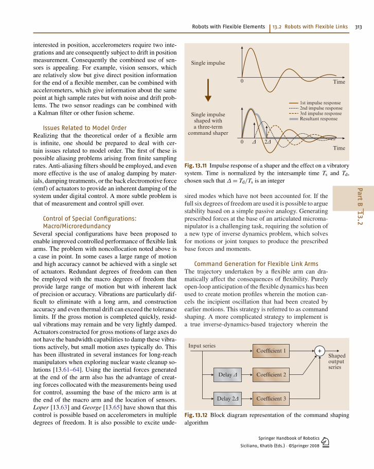
Springer Handbook of Robotics
Siciliano, Khatib (Eds.) · ©Springer 2008 1
Robots with Flexible Elements 13.2 Robots with Flexible Links 313
interested in position, accelerometers require two inte-grations and are consequently subject to drift in positionmeasurement. Consequently the combined use of sen-sors is appealing. For example, vision sensors, whichare relatively slow but give direct position informationfor the end of a flexible member, can be combined withaccelerometers, which give information about the samepoint at high sample rates but with noise and drift prob-lems. The two sensor readings can be combined witha Kalman filter or other fusion scheme.
Issues Related to Model OrderRealizing that the theoretical order of a flexible armis infinite, one should be prepared to deal with cer-tain issues related to model order. The first of these ispossible aliasing problems arising from finite samplingrates. Anti-aliasing filters should be employed, and evenmore effective is the use of analog damping by mater-ials, damping treatments, or the back electromotive force(emf) of actuators to provide an inherent damping of thesystem under digital control. A more subtle problem isthat of measurement and control spill over.
Control of Special Configurations:Macro/Microredundancy
Several special configurations have been proposed toenable improved controlled performance of flexible linkarms. The problem with noncollocation noted above isa case in point. In some cases a large range of motionand high accuracy cannot be achieved with a single setof actuators. Redundant degrees of freedom can thenbe employed with the macro degrees of freedom thatprovide large range of motion but with inherent lackof precision or accuracy. Vibrations are particularly dif-ficult to eliminate with a long arm, and constructionaccuracy and even thermal drift can exceed the tolerancelimits. If the gross motion is completed quickly, resid-ual vibrations may remain and be very lightly damped.Actuators constructed for gross motions of large axes donot have the bandwidth capabilities to damp these vibra-tions actively, but small motion axes typically do. Thishas been illustrated in several instances for long-reachmanipulators when exploring nuclear waste cleanup so-lutions [13.61–64]. Using the inertial forces generatedat the end of the arm also has the advantage of creat-ing forces collocated with the measurements being usedfor control, assuming the base of the micro arm is atthe end of the macro arm and the location of sensors.Loper [13.63] and George [13.65] have shown that thiscontrol is possible based on accelerometers in multipledegrees of freedom. It is also possible to excite unde-
0
Single impulse
Single impulseshaped witha three-term
command shaper
Δ 2ΔTime
0 Time
1st impulse response2nd impulse response3rd impulse responseResultant response
Fig. 13.11 Impulse response of a shaper and the effect on a vibratorysystem. Time is normalized by the intersample time Ts and Td,chosen such that Δ = Td/Ts is an integer
sired modes which have not been accounted for. If thefull six degrees of freedom are used it is possible to arguestability based on a simple passive analogy. Generatingprescribed forces at the base of an articulated microma-nipulator is a challenging task, requiring the solution ofa new type of inverse dynamics problem, which solvesfor motions or joint torques to produce the prescribedbase forces and moments.
Command Generation for Flexible Link ArmsThe trajectory undertaken by a flexible arm can dra-matically affect the consequences of flexibility. Purelyopen-loop anticipation of the flexible dynamics has beenused to create motion profiles wherein the motion can-cels the incipient oscillation that had been created byearlier motions. This strategy is referred to as commandshaping. A more complicated strategy to implement isa true inverse-dynamics-based trajectory wherein the
Coefficient 1Input series
Shapedoutputseries
Coefficient 2
Coefficient 3
Delay Δ
Delay 2Δ
Fig. 13.12 Block diagram representation of the command shapingalgorithm
PartB
13.2
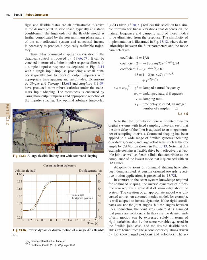
Springer Handbook of Robotics
Siciliano, Khatib (Eds.) · ©Springer 20081
314 Part B Robot Structures
rigid and flexible states are all orchestrated to arriveat the desired point in state space, typically at a staticequilibrium. The high order of the flexible model isfurther complicated by the non-minimum-phase natureof the non-collocated system and noncausal inverseis necessary to produce a physically realizable trajec-tory.
Time delay command shaping is a variation of thedeadbeat control introduced by [13.66, 67]. It can becouched in terms of a finite impulse response filter witha simple impulse response as depicted in Fig. 13.11with a single input impulse producing a small num-ber (typically two to four) of output impulses withappropriate time spacing and amplitudes. Extensionsby Singer and Seering [13.68] and Singhose [13.69]have produced more-robust varieties under the trade-mark Input Shaping. The robustness is enhanced byusing more output impulses and appropriate selection ofthe impulse spacing. The optimal arbitrary time-delay
Fig. 13.13 A large flexible linking arm with command shaping
Joint angleEnd point position
0 0.2 0.4 0.6 0.8 1 1.2 1.4 1.6 1.8 2 2.2
Joint angle (rad) Displacement (in)
Time (s)
Generated joint trajectory
1.06
0.85
0.64
0.43
0.21
0
–0.21
50
40
30
20
10
0
–10
Fig. 13.14 Inverse dynamics driven motion of a single-link flexiblearm
(OAT) filter [13.70, 71] reduces this selection to a sim-ple formula for linear vibrations that depends on thenatural frequency and damping ratio of those modesto be eliminated from the response. The simplicity ofimplementation is illustrated in Fig. 13.12, where the re-lationships between the filter parameters and the modeparameters are
coefficient 1 = 1/M
coefficient 2 = −(2 cos ωdTd e−ζωnTd )/M
coefficient 3 = (e−2ζωnTd )/M
M = 1−2 cos ωdTd e−ζωnTd
+ e−2ζωnTd
ωd = ωn
√1− ζ2 = damped natural frequency
ωn = undamped natural frequency
ζ = damping ratio
Td = time delay selected, an integernumber of samples = Δ
(13.82)
Note that the formulation here is oriented towardsdigital systems with fixed sampling intervals such thatthe time delay of the filter is adjusted to an integer num-ber of sampling intervals. Command shaping has beenapplied to a wide range of flexible systems includingdisk drives, cranes, and large robot arms, such as the ex-ample by CAMotion shown in Fig. 13.13. Note that thisexample contains a flexible drive belt, effectively a flex-ible joint, as well as flexible links that contribute to thecompliance of the lowest mode that is quenched with anOAT filter.
Adaptive versions of command shaping have alsobeen demonstrated. A version oriented towards repeti-tive motion applications is presented in [13.72].
In contrast to the scant system knowledge requiredfor command shaping, the inverse dynamics of a flex-ible arm requires a great deal of knowledge about thesystem. The creation of an appropriate model was dis-cussed above. An assumed modes model, for example,is well adapted to inverse dynamics if the rigid coordi-nates are not the joint angles, but the angles betweenlines connecting the joint axes (where it is assumedthat joints are rotational). In this case the desired end-of-arm motion can be expressed solely in terms ofrigid variables, that is, the same variables qd used inthe flexible joint case, and the desired flexible vari-ables are found from the second-order equations drivenby the known rigid positions and velocities. The re-
PartB
13.2
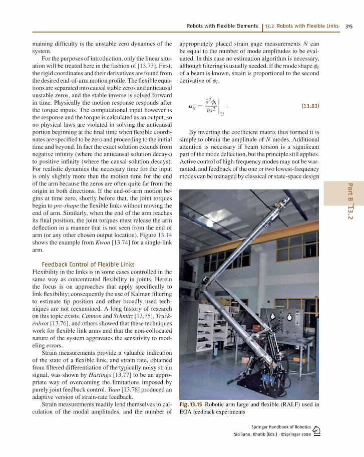
Springer Handbook of Robotics
Siciliano, Khatib (Eds.) · ©Springer 2008 1
Robots with Flexible Elements 13.2 Robots with Flexible Links 315
maining difficulty is the unstable zero dynamics of thesystem.
For the purposes of introduction, only the linear situ-ation will be treated here in the fashion of [13.73]. First,the rigid coordinates and their derivatives are found fromthe desired end-of-arm motion profile. The flexible equa-tions are separated into causal stable zeros and anticausalunstable zeros, and the stable inverse is solved forwardin time. Physically the motion response responds afterthe torque inputs. The computational input however isthe response and the torque is calculated as an output, sono physical laws are violated in solving the anticausalportion beginning at the final time when flexible coordi-nates are specified to be zero and proceeding to the initialtime and beyond. In fact the exact solution extends fromnegative infinity (where the anticausal solution decays)to positive infinity (where the causal solution decays).For realistic dynamics the necessary time for the inputis only slightly more than the motion time for the endof the arm because the zeros are often quite far from theorigin in both directions. If the end-of-arm motion be-gins at time zero, shortly before that, the joint torquesbegin to pre-shape the flexible links without moving theend of arm. Similarly, when the end of the arm reachesits final position, the joint torques must release the armdeflection in a manner that is not seen from the end ofarm (or any other chosen output location). Figure 13.14shows the example from Kwon [13.74] for a single-linkarm.
Feedback Control of Flexible LinksFlexibility in the links is in some cases controlled in thesame way as concentrated flexibility in joints. Hereinthe focus is on approaches that apply specifically tolink flexibility; consequently the use of Kalman filteringto estimate tip position and other broadly used tech-niques are not reexamined. A long history of researchon this topic exists. Cannon and Schmitz [13.75], Truck-enbrot [13.76], and others showed that these techniqueswork for flexible link arms and that the non-collocatednature of the system aggravates the sensitivity to mod-eling errors.
Strain measurements provide a valuable indicationof the state of a flexible link, and strain rate, obtainedfrom filtered differentiation of the typically noisy strainsignal, was shown by Hastings [13.77] to be an appro-priate way of overcoming the limitations imposed bypurely joint feedback control. Yuan [13.78] produced anadaptive version of strain-rate feedback.
Strain measurements readily lend themselves to cal-culation of the modal amplitudes, and the number of
appropriately placed strain gage measurements N canbe equal to the number of mode amplitudes to be eval-uated. In this case no estimation algorithm is necessary,although filtering is usually needed. If the mode shape φiof a beam is known, strain is proportional to the secondderivative of φi ,
αij = ∂2φi
∂x2
∣∣∣∣x j
. (13.83)
By inverting the coefficient matrix thus formed it issimple to obtain the amplitude of N modes. Additionalattention is necessary if beam torsion is a significantpart of the mode deflection, but the principle still applies.Active control of high-frequency modes may not be war-ranted, and feedback of the one or two lowest-frequencymodes can be managed by classical or state-space design
Fig. 13.15 Robotic arm large and flexible (RALF) used inEOA feedback experiments
PartB
13.2
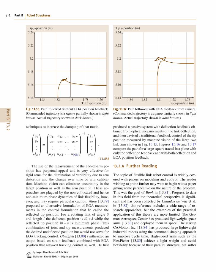
Springer Handbook of Robotics
Siciliano, Khatib (Eds.) · ©Springer 20081
316 Part B Robot Structures
–1.84 –1.82 –1.8 –1.78 –1.76
Tip y-position (m)
Tip x-position (m)
5.24
5.22
5.2
5.18
5.16
5.14
Fig. 13.16 Path followed without EOA position feedback.(Commanded trajectory is a square partially shown in lightbrown. Actual trajectory shown in dark brown.)
techniques to increase the damping of that mode
⎛⎜⎜⎜⎜⎝
δ1
δ2...
δN
⎞⎟⎟⎟⎟⎠ =
⎛⎜⎜⎜⎜⎝
α11 α12 . . . α1N
α21 α22 . . . α2N...
.... . .
...
αN1 αN2 . . . αNN
⎞⎟⎟⎟⎟⎠
−1 ⎛⎜⎜⎜⎜⎝
ε1
ε2...
εN
⎞⎟⎟⎟⎟⎠ .
(13.84)
The use of the measurement of the end-of-arm po-sition has perpetual appeal and is very effective forrigid arms for the elimination of variability due to armdistortion and the change over time of arm calibra-tion. Machine vision can eliminate uncertainty in thetarget position as well as the arm position. These ap-proaches are plagued by the non-collocated and hencenon-minimum-phase dynamics of link flexibility, how-ever, and may require particular caution. Wang [13.79]proposed an alternative formulation of EOA measure-ments in the control formulation that he called thereflected tip position. For a rotating link of angle θ
and length l the deflected position is lθ + δ while thereflected tip position lθ − δ is minimum phase. Thiscombination of joint and tip measurements producedthe desired undeflected position but would not serve forEOA tracking control. Obergfell [13.80] synthesized anoutput based on strain feedback combined with EOAposition that allowed tracking control as well. He first
–1.84 –1.82 –1.8 –1.78 –1.76
Tip y-position (m)
Tip x-position (m)
5.24
5.22
5.2
5.18
5.16
5.14
Fig. 13.17 Path followed with EOA feedback from camera.(Commanded trajectory is a square partially shown in lightbrown. Actual trajectory shown in dark brown.)
produced a passive system with deflection feedback ob-tained from optical measurements of the link deflection,and then devised a traditional feedback control of the tipposition measured by machine vision of the large twolink arm shown in Fig. 13.15. Figures 13.16 and 13.17compare the path for a large square traced in a plane withonly the deflection feedback and with both deflection andEOA position feedback.
13.2.4 Further Reading
The topic of flexible link robot control is widely cov-ered with papers on modeling and control. The readerwishing to probe further may want to begin with a papergiving some perspective on the nature of the problem.This was the goal of Book in [13.81]. Progress to datein this field from the theoretical perspective is signifi-cant and has been collected by Canudas de Witt et al.in [13.82]; this reference includes a wide range of re-search approaches, but the examples of the practicalapplication of this theory are more limited. The Ger-man Aerospace Center has produced lightweight spacearms [13.83] and deployed them in space. The startupCAMotion Inc. [13.84] has produced large lightweightindustrial robots using the command-shaping approachto improve cycle time. High-speed arms such as theFlexPicker [13.85] achieve a light weight and avoidflexibility because of their parallel structure, but suffer
PartB
13.2
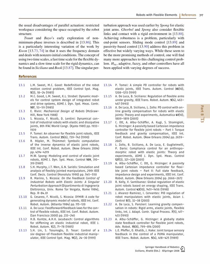
Springer Handbook of Robotics
Siciliano, Khatib (Eds.) · ©Springer 2008 1
Robots with Flexible Elements References 317
the usual disadvantages of parallel actuation: restrictedworkspace considering the space occupied by the robotstructure.
Trautt and Bayo’s early exploration of non-minimum-phase inverses is described in [13.86]. Thisis a particularly interesting variation of the work byKwon [13.73, 74] in that it uses the frequency domainand deals with nonzero initial conditions. The concept ofusing two time scales, a fast time scale for the flexible dy-namics and a slow time scale for the rigid dynamics, canbe found in Siciliano and Book [13.87]. The singular per-
turbation approach was used earlier by Spong for elasticjoint arms. Ghorbel and Spong also consider flexiblelinks and contact with a rigid environment in [13.88].Achieving robustness is a problem, particularly withend-point sensors. Sliding mode control [13.89] andpassivity-based control [13.90] address this problem ineffective but widely varying ways. While these seem tobe the more promising methods of control, one will findmany more approaches to this challenging control prob-lem. H∞, adaptive, fuzzy, and other controllers have allbeen applied with varying degrees of success.
References
13.1 L.M. Sweet, M.C. Good: Redefinition of the robotmotion control problem, IEEE Control Syst. Mag.5(3), 18–24 (1985)
13.2 M.C. Good, L.M. Sweet, K.L. Strobel: Dynamic mod-els for control system design of integrated robotand drive systems, ASME J. Dyn. Syst. Meas. Contr.107, 53–59 (1985)
13.3 E. Rivin: Mechanical Design of Robots (McGraw-Hill, New York 1988)
13.4 S. Nicosia, F. Nicolò, D. Lentini: Dynamical con-trol of industrial robots with elastic and dissipativejoints, 8th IFAC World Congr. (Kyoto 1981) pp. 1933–1939
13.5 P. Tomei: An observer for flexible joint robots, IEEETrans. Autom. Control 35(6), 739–743 (1990)
13.6 R. Höpler, M. Thümmel: Symbolic computationof the inverse dynamics of elastic joint robots,IEEE Int. Conf. Robot. Autom. (New Orleans 2004)pp. 4314–4319
13.7 M.W. Spong: Modeling and control of elastic jointrobots, ASME J. Dyn. Syst. Meas. Control 109, 310–319 (1987)
13.8 S.H. Murphy, J.T. Wen, G.N. Saridis: Simulation andanalysis of flexibly jointed manipulators, 29th IEEEConf. Decis. Control (Honolulu 1990) pp. 545–550
13.9 R. Marino, S. Nicosia: On the Feedback Control ofIndustrial Robots with Elastic Joints: A SingularPerturbation Approach (Dipartimento di IngegneriaElettronica, Univ. Rome Tor Vergata, Rome 1984),Rep. R-84.01
13.10 G. Cesareo, F. Nicolò, S. Nicosia: DYMIR: A code forgenerating dynamic model of robots, IEEE Int. Conf.Robot. Autom. (Atlanta 1984) pp. 115–120
13.11 A. De Luca: Feedforward/feedback laws for the con-trol of flexible robots, IEEE Int. Conf. Robot. Autom.(San Francisco 2000) pp. 233–240
13.12 H.B. Kuntze, A.H.K. Jacubasch: Control algorithmsfor stiffening an elastic industrial robot, IEEE J.Robot. Autom. 1(2), 71–78 (1985)
13.13 S.H. Lin, S. Tosunoglu, D. Tesar: Control of asix-degree-of-freedom flexible industrial manip-ulator, IEEE Control Syst. Mag. 11(2), 24–30 (1991)
13.14 P. Tomei: A simple PD controller for robots withelastic joints, IEEE Trans. Autom. Control 36(10),1208–1213 (1991)
13.15 A. De Luca, B. Siciliano: Regulation of flexible armsunder gravity, IEEE Trans. Robot. Autom. 9(4), 463–467 (1993)
13.16 A. De Luca, B. Siciliano, L. Zollo: PD control with on-line gravity compensation for robots with elasticjoints: Theory and experiments, Automatica 41(10),1809–1819 (2005)
13.17 C. Ott, A. Albu-Schäffer, A. Kugi, S. Stramigioli,G. Hirzinger: A passivity based Cartesian impedancecontroller for flexible joint robots – Part I: Torquefeedback and gravity compensation, IEEE Int.Conf. Robot. Autom. (New Orleans 2004) pp. 2659–2665
13.18 L. Zollo, B. Siciliano, A. De Luca, E. Guglielmelli,P. Dario: Compliance control for an anthropo-morphic robot with elastic joints: Theory andexperiments, ASME J. Dyn. Syst. Meas. Control127(3), 321–328 (2005)
13.19 A. Albu-Schäffer, C. Ott, G. Hirzinger: A passivitybased Cartesian impedance controller for flexi-ble joint robots – Part II: Full state feedback,impedance design and experiments, IEEE Int. Conf.Robot. Autom. (New Orleans 2004) pp. 2666–2672
13.20 R. Kelly, V. Santibanez: Global regulation of elasticjoint robots based on energy shaping, IEEE Trans.Autom. Control 43(10), 1451–1456 (1998)
13.21 J. Alvarez-Ramirez, I. Cervantes: PID regulation ofrobot manipulators with elastic joints, Asian J.Control 5(1), 32–38 (2003)
13.22 A. De Luca, S. Panzieri: Learning gravity compen-sation in robots: Rigid arms, elastic joints, flexiblelinks, Int. J. Adapt. Contr. Signal Process. 7(5), 417–433 (1993)
13.23 A. Albu-Schäffer, G. Hirzinger: A globally stablestate feedback controller for flexible joint robots,Adv. Robot. 15(8), 799–814 (2001)
13.24 L.E. Pfeffer, O. Khatib, J. Hake: Joint torque sensoryfeedback in the control of a PUMA manipulator,IEEE Trans. Robot. Autom. 5(4), 418–425 (1989)
PartB
13
Springer Handbook of Robotics
Siciliano, Khatib (Eds.) · ©Springer 20081
318 Part B Robot Structures
13.25 M. Hashimoto, Y. Kiyosawa, R.P. Paul: A torquesensing technique for robots with harmonic drives,IEEE Trans. Robot. Autom. 9(1), 108–116 (1993)
13.26 T. Lin, A.A. Goldenberg: Robust adaptive controlof flexible joint robots with joint torque feed-back, IEEE Int. Conf. Robot. Autom. (Nagoya 1995)pp. 1229–1234
13.27 M.G. Forrest-Barlach, S.M. Babcock: Inverse dy-namics position control of a compliant manipu-lator, IEEE J. Robot. Autom. 3(1), 75–83 (1987)
13.28 K.P. Jankowski, H. Van Brussel: An approach todiscrete inverse dynamics control of flexible-jointrobots, IEEE Trans. Robot. Autom. 8(5), 651–658(1992)
13.29 W.M. Grimm: Robustness analysis of nonlinear de-coupling for elastic-joint robots, IEEE Trans. Robot.Autom. 6(3), 373–377 (1990)
13.30 A. De Luca, R. Farina, P. Lucibello: On the controlof robots with visco-elastic joints, IEEE Int. Conf.Robot. Autom. (Barcelona 2005) pp. 4297–4302
13.31 A. De Luca: Decoupling and feedback lineariza-tion of robots with mixed rigid/elastic joints, Int.J. Robust Nonlin. Contr. 8(11), 965–977 (1998)
13.32 A. De Luca, B. Siciliano: Inversion-based nonlinearcontrol of robot arms with flexible links, AIAA J.Guid. Control Dyn. 16(6), 1169–1176 (1993)
13.33 A. De Luca: Dynamic control of robots with jointelasticity, IEEE Int. Conf. Robot. Autom. (Philadel-phia 1988) pp. 152–158
13.34 S. Nicosia, P. Tomei: On the feedback linearizationof robots with elastic joints, 27th IEEE Conf. Decis.Control (Austin 1988) pp. 180–185
13.35 A. De Luca, P. Lucibello: A general algorithm for dy-namic feedback linearization of robots with elasticjoints, IEEE Int. Conf. Robot. Autom. (Leuven 1998)pp. 504–510
13.36 K. Khorasani, P.V. Kokotovic: Feedback lineariza-tion of a flexible manipulator near its rigid bodymanifold, Syst. Control Lett. 6, 187–192 (1985)
13.37 M.W. Spong, K. Khorasani, P.V. Kokotovic: An in-tegral manifold approach to the feedback controlof flexible joint robots, IEEE J. Robot. Autom. 3(4),291–300 (1987)
13.38 S. Nicosia, P. Tomei: Design of global tracking con-trollers for flexible-joint robots, J. Robot. Syst.10(6), 835–846 (1993)
13.39 B. Brogliato, R. Ortega, R. Lozano: Global trackingcontrollers for flexible-joint manipulators: A com-parative study, Automatica 31(7), 941–956 (1995)
13.40 M.W. Spong: Adaptive control of flexible joint ma-nipulators, Syst. Control Lett. 13(1), 15–21 (1989)
13.41 R. Lozano, B. Brogliato: Adaptive control of robotmanipulators with flexible joints, IEEE Trans. Au-tom. Control 37(2), 174–181 (1992)
13.42 H. Sira-Ramirez, M.W. Spong: Variable structurecontrol of flexible joint manipulators, Int. Robot.Autom. 3(2), 57–64 (1988)
13.43 A. De Luca, G. Ulivi: Iterative learning control ofrobots with elastic joints, IEEE Int. Conf. Robot.Autom. (Nice 1992) pp. 1920–1926
13.44 S. Nicosia, P. Tomei, A. Tornambè: A nonlinear ob-server for elastic robots, IEEE J. Robot. Autom. 4(1),45–52 (1988)
13.45 S. Nicosia, P. Tomei: A method for the state es-timation of elastic joint robots by global positionmeasurements, Int. J. Adapt. Contr. Signal Process.4(6), 475–486 (1990)
13.46 A. De Luca, D. Schröder, M. Thümmel: Anacceleration-based state observer for robot ma-nipulators with elastic joints, IEEE Int. Conf. Robot.Autom. (Rome 2007) pp. 3817–3823
13.47 M.W. Spong: On the force control problem for flex-ible joint manipulators, IEEE Trans. Autom. Control34(1), 107–111 (1989)
13.48 J.K. Mills: Stability and control of elastic-jointrobotic manipulators during constrained-motiontasks, IEEE Trans. Robot. Autom. 8(1), 119–126 (1992)
13.49 K.P. Jankowski, H.A. El Maraghy: Dynamic de-coupling for hybrid control of rigid-/flexible-jointrobots interacting with the environment, IEEETrans. Robot. Autom. 8(5), 519–534 (1992)
13.50 T. Lin, A.A. Goldenberg: A unified approach tomotion and force control of flexible joint robots,IEEE Int. Conf. Robot. Autom. (Minneapolis 1996)pp. 1115–1120
13.51 W. Book, O. Maizza-Neto, D.E. Whitney: FeedbackControl of Two Beam, Two Joint Systems with Dis-tributed Flexibility, ASME J. Dyn. Syst. Meas. Control97(4), 424–431 (1975)
13.52 W. Book: Characterization of Strength and Stiff-ness Constraints on Manipulator Control, In: Theoryand Practice of Robots and Manipulators (Elsevier,Amsterdam 1977) pp. 37–45
13.53 T.E. Alberts, W. Book, S. Dickerson: Experimentsin Augmenting Active Control of a Flexible Struc-ture with Passive Damping, AIAA 24th AerospaceSciences Meeting (Reno 1986)
13.54 T. Bailey, J.E. Hubbard Jr.: Distributed piezoelectric-polymer active vibration control of a cantileverbeam, J. Guid. Control Dyn. 8(5), 605–611 (1985)
13.55 W. Book, V. Sangveraphunsiri, S. Le: The BracingStrategy for Robot Operation, Joint IFToMM-CISMSymposium on the Theory of Robots and Manip-ulators (RoManSy) (Udine 1984)
13.56 W. Book: Analysis of Massless Elastic Chains withServo Controlled Joints, ASME J. Dyn. Syst. Meas.Control 101(3), 187–192 (1979)
13.57 E.C. Pestel, F.A. Leckie: Matrix Methods in Elas-tomechanics (McGraw Hill, New York 1963)
13.58 R. Krauss: Transfer Matrix Modeling. Ph.D. Thesis(School of Mechanical Engineering, Georgia Insti-tute of Technology 2006)
13.59 W.J. Book: Modeling, Design and Control of Flexi-ble Manipulator Arms. Ph.D. Thesis (Department of
PartB
13
Springer Handbook of Robotics
Siciliano, Khatib (Eds.) · ©Springer 2008 1
Robots with Flexible Elements References 319
Mechanical Engineering, Massachusetts Institute ofTechnology 1974)
13.60 W. Book: Recursive Lagrangian Dynamics of Flex-ible Manipulators, Int. J. Robot. Res. 3(3), 87–106(1984)
13.61 W.J. Book, S.H. Lee: Vibration Control of a LargeFlexible Manipulator by a Small Robotic Arm, Proc.Am. Contr. Conf. (Pittsburgh 1989) pp. 1377–1380
13.62 J. Lew, S.-M. Moon: A Simple Active Damping Con-trol for Compliant Base Manipulators, IEEE/ASMETrans. Mechatronics 2, 707–714 (1995)
13.63 W.J. Book, J.C. Loper: Inverse Dynamics for Com-manding Micromanipulator Inertial Forces to DampMacromanipulator Vibration, IEEE, Robot Societyof Japan International Conference on IntelligentRobots and Systems (Kyongju 1999)
13.64 I. Sharf: Active Damping of a Large Flexible Ma-nipulator with a Short-Reach Robot, Proc. Ofthe American Control Conference (Seattle 1995)pp. 3329–3333
13.65 L. George, W.J. Book: Inertial Vibration DampingControl of a Flexible Base Manipulator, IEEE/ASMETransactions on Mechatronics (2003)
13.66 J.F. Calvert, D.J. Gimpel: Method and Apparatus forControl of System Output in Response to SystemInput, Patent 2801351 (1957)
13.67 O.J.M. Smith: Feedback Control Systems (McGrawHill, New York 1958)
13.68 N. Singer, W.P. Seering: Preshaping Command In-puts to Reduce System Vibration, ASME J. Dyn. Syst.Meas. Contr. 112(1), 76–82 (1990)
13.69 W. Singhose, W. Seering, N. Singer: Residual Vibra-tion Reduction Using Vector Diagrams to GenerateShaped Inputs, J. Mech. Des. 2, 654–659 (1994)
13.70 D.P. Magee, W.J. Book: The Application of InputShaping to a System with Varying Parameters, Pro-ceedings of the 1992 Japan-U.S.A. Symposium onFlexible Automation (San Francisco 1992) pp. 519–526
13.71 D.P. Magee, W.J. Book: Optimal Arbitrary Time-delay (OAT) Filter and Method to MinimizeUnwanted System Dynamics, Patent 6078844(2000)
13.72 S. Rhim, W.J. Book: Noise Effect on Time-domainAdaptive Command Shaping Methods for FlexibleManipulator Control, IEEE Trans. Control Syst. Tech-nol. 9(1), 84–92 (2001)
13.73 D.-S. Kwon,, W.J. Book: A Time-Domain InverseDynamic Tracking Control of a Single-Link FlexibleManipulator, J. Dyn. Syst. Meas. Control 116, 193–200 (1994)
13.74 D.S. Kwon: An Inverse Dynamic Tracking Control fora Bracing Flexible Manipulator. Ph.D. Thesis (School
of Mechanical Engineering, Georgia Institute ofTechnology 1991)
13.75 R.H. Cannon, E. Schmitz: Initial Experiments on theEnd-Point Control of a Flexible One-Link Robot, Int.J. Robot. Res. 3(3), 62–75 (1984)
13.76 A. Truckenbrot: Modeling and Control of Flexi-ble Manipulator Structures, Proc. 4th CISM-IFToMMRo.Man.Sy. (Zaborow 1981) pp. 90–101
13.77 G.G. Hastings, W.J. Book: Reconstruction andRobust Reduced-Order Observation of FlexibleVariables, ASME Winter Annual Meeting (Anaheim1986)
13.78 B.S. Yuan, J.D. Huggins, W.J. Book: Small MotionExperiments with a Large Flexible Arm with StrainFeedback, Proceedings of the 1989 American Con-trol Conference (Pittsburgh 1989) pp. 2091–2095
13.79 D. Wang, M. Vidyasagar: Passive Control of a StiffFlexible Link, Int. J. Robot. Res. 11, 572–578 (1992)
13.80 K. Obergfell, W.J. Book: Control of Flexible Ma-nipulators Using Vision and Modal Feedback,Proceedings of the ICRAM (Istanbul 1995)
13.81 W.J. Book: Controlled Motion in an Elastic World,ASME J. Dyn. Syst. Meas. Control 2B, 252–261 (1993),50th Anniversary Issue
13.82 C. Canudas-de-Wit, B. Siciliano, G. Bastin (eds.):Theory of Robot Control (Springer, Berlin, Heidel-berg 1996)
13.83 G. Hirzinger, N. Sporer, J. Butterfass, M. Greben-stein: Torque-Controlled Lightweight Arms andArticulated Hands: Do We Reach Technological Lim-its Now?, Int. J. Robot. Res. 23(4,5), 331–340 (2004)
13.84 Camotion Inc.: http://www.camotion.com (Camo-tion Inc., Atlanta 2007)
13.85 B. Rooks: High Speed Delivery and Low Cost fromNew ABB Packaging Robot, Ind. Robot. Int. J. 26(4),267–275 (1999)
13.86 T. Trautt, E. Bayo: Inverse Dynamics of Non-Minimum Phase Systems with Non-Zero InitialConditions, Dyn. Control 7(1), 49–71 (1997)
13.87 B. Siciliano, W. Book: A Singular PerturbationApproach to Control of Lightweight Flexible Ma-nipulators, Int. J. Robot. Res. 7(4), 79–90 (1988)
13.88 F. Ghorbel, M.W. Spong: Singular PerturbationModel of Robots with Elastic Joints and ElasticLinks Constrained by a Rigid Environment, J. Intell.Robot. Syst. 22(2), 143–152 (1998)
13.89 J. Guldner, J. Shi, V. Utkin: Sliding Mode Control inElectromechanical Systems (Taylor Francis, London,Philadelphia 1999)
13.90 J.-H. Ryu, D.-S. Kwon, B. Hannaford: Control ofa Flexible Manipulator with Noncollocated Feed-back: Time-domain Passivity Approach, IEEE Trans.Robot. 20(4), 776–780 (2004 )
PartB
13