Embed Size (px)
Citation preview
1 Copyright © 2015 by ASME
Proceedings of ASME 2015 DSCC ASME Dynamic Systems and Control Conference
October 28-30, 2015, Columbus, Ohio, USA
ROBUST ADAPTIVE IMPEDANCE CONTROL OF A PROSTHETIC LEG
Vahid Azimi Department of Electrical and
Computer Engineering, Cleveland State University,
Cleveland, OH, USA Email: [email protected]
Dan Simon Department of Electrical and
Computer Engineering, Cleveland State University,
Cleveland, OH, USA Email: [email protected]
Hanz Richter Department of Mechanical
Engineering, Cleveland State University,
Cleveland, OH, USA Email: [email protected]
ABSTRACT
We propose a regressor-based nonlinear robust model
reference adaptive impedance controller for an active prosthetic
leg for a transfemoral amputee. We use an adaptive control term
to estimate the uncertain parameters of the system, and a robust
control term so the system trajectories converge to a sliding
manifold and exhibit robustness to variations of ground reaction
force (GRF). The sliding mode boundary layer not only
compromises between control chattering and tracking
performance, but also bounds the parameter adaptations to
prevent unfavorable parameter drift. We prove the stability of the
closed-loop system with Lyapunov stability theory and the
Barbalat lemma. We use particle swarm optimization (PSO) to
optimize the design parameters of the controller and the
adaptation law. The PSO cost function is comprised of control
signal magnitudes and tracking errors. PSO achieves a 22%
improvement in the objective function. The acceleration-free
regressor form of the system removes the need to measure the
joint accelerations, which would otherwise introduce noise in the
system. Finally, we present simulation results to validate the
effectiveness of the controller. We achieve accurate tracking of
joint displacements and velocities for both nominal and
perturbed values of the system parameters. Variations of ±30%
on the system parameters results in an increase of the cost
function by only 10%whichconfirms the robustness of the
proposed controller.
KEYWORDS Robust control, model reference adaptive control, impedance
control, sliding mode control, prosthetics, particle swarm
optimization
INTRODUCTION
The number of people with limb loss in the United States is
estimated at about two million. Amputation has several main
causes, including accident, cancer, vascular disease, other
disease, birth defect, and paralysis [1]-[2]. Different types of
amputation include transtibial (below the knee), transfemoral
(above the knee), foot amputations, and hip and knee
disarticulations (amputation through the joint). Transfemoral
amputees can use prosthetic legs in an attempt to restore a normal
walking gait.
There are three types of prosthetic legs: passive (no
electronic control), active (motor control), and semi-active
(control without motors). Technology has provided advanced
prosthetic legs for amputees so that they can remain active and
so that they can emulate able-bodied gait. Compared to passive
and semi-active prostheses, active prostheses enable more
natural walking.
The Power Knee was the first commercially available active
transfemoral prosthesis. A combination knee / ankle prosthesis,
both joints of which are active, was recently developed at
Vanderbilt University and is in the process of commercialization.
Many researchers have recently concentrated on the design and
control of these and other active prostheses [3-7]. Recent years
have witnessed numerous advancements in the development of
control and modeling approaches for prosthetic legs [8-10].
A prosthesis can be viewed as a robotic system. A robot’s
environment and the robot itself can be viewed as a mechanical
admittance and impedance respectively. This motivates the
development of impedance control [11]. However, modeling
inaccuracies are unavoidable. Robust controllers can be used to
reduce these effects on the performance and stability of the
system [12-13]. Robust controllers try to achieve a certain level
of performance in the presence of modeling uncertainties,
whereas adaptive controllers try to achieve performance with
learning and adaptation. Adaptive controllers may be preferable
to non-adaptive robust controllers because adaptive controllers
can handle system uncertainties that change with time. Non-
adaptive robust controllers require a priori knowledge of the
bounds of the parameter perturbations, whereas adaptive
approaches do not.
The aforementioned advantages of adaptive control, along
with the availability of able-bodied human impedance properties
and uncertain model parameters, has given rise to impedance
model reference adaptive control for robotics [14-16]. Pure
adaptive control approaches may become unstable when
2 Copyright © 2015 by ASME
disturbances, unmodeled dynamics, or external forces affect the
system. Robust control can alleviate instabilities in these cases
[17-19]. Several adaptive control schemes and sliding surface
theories have also been proposed for robotics [20-23].
The contribution of this research is the design of a nonlinear
robust model reference adaptive impedance controller for a
prosthetic leg for transfemoral amputees. We use robust adaptive
control to deal with parameter uncertainties and GRF variations
so that the closed-loop system converges to a target impedance
model. Among related research [14-16], our work has the most
similarity to the controller presented in [15]. New contributions
in this paper include blending adaptive and robust control not
only to reduce the effects of unknown parameters on system
performance and stability, but also to obtain good robustness
against GRF variations (environment interaction). We define a
first-order sliding surface so the system trajectories reach the
sliding manifold 𝑠 = 0 in finite time, given a relevant reaching
condition. We design a control law comprising an adaptive
control term to account for uncertain parameters, and a robust
control term to account for the aforementioned reaching
condition and GRF variations. We extend previous work [15] by
defining a trajectory 𝑠∆ to balance control chattering and tracking
accuracy, and to bound the parameter adaptation. We define a
boundary layer to stop parameter adaptation when tracking
errors reach a satisfactory level. We then prove the stability of
the closed-loop system via Barbalat’s lemma by defining a
suitable Lyapunov function, which leads to a stable adaptation
law. Furthermore, we use PSO to optimize the control design
parameters. The PSO cost function includes control signal
magnitudes and tracking errors, and PSO reduces the cost
function by 22%. Numerical results show that the proposed
system has good robustness to system uncertainties. When we
change the system parameters by −30% and +30%, the total cost
increases by only 7.7% and 10% respectively, and the tracking
performance component of the cost increases by 10.7% and 39%
respectively.
The following section describes the dynamic model of the
prosthetic leg. In the next section we design the controller and
prove its stability. The next section presents simulation results
and robustness results. The final section includes discussion and
concluding remarks.
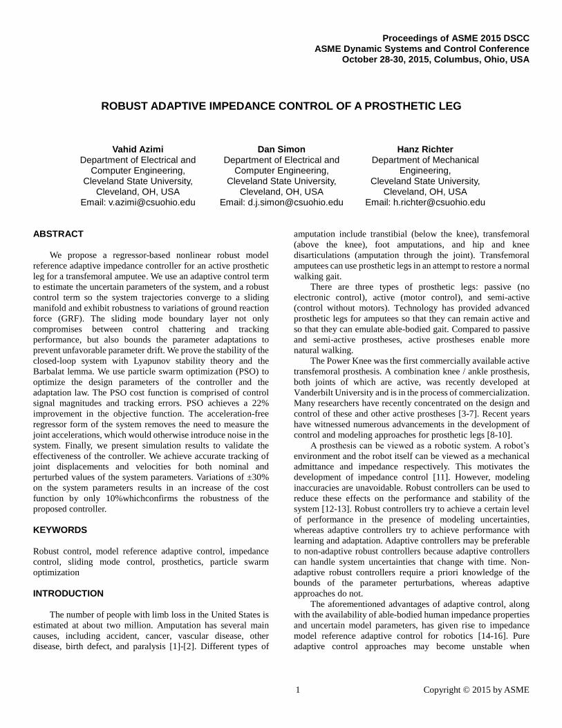
PROSTHETIC LEG MODEL
We present a model for the prosthetic leg with three rigid
links and three degrees of freedom. The prosthetic component is
modeled as an active transfemoral (above-knee) prosthesis. This
proposed model has a prismatic-revolute-revolute (PRR) joint
structure as illustrated in Fig. 1. The vertical degree of freedom
represents human hip motion, the first rotational axis represents
human angular thigh motion, and the second rotational axis
represents the prosthetic knee angular motion. Human hip and
thigh motion are emulated by a prosthesis test robot [9], [10],
[24].
Fig. 1. Prosthetic leg model with rigid ankle
The three degree-of-freedom model can be written as
follows [9]:
𝑀�̈� + 𝐶�̇� + 𝑔 + 𝑅 = 𝑢 − 𝑇𝑒 (1)
where 𝑞𝑇 = [𝑞1 𝑞2 𝑞3] is the vector of generalized joint
displacements (𝑞1is the vertical displacement, 𝑞2 is the thigh
angle, and 𝑞3 is the knee angle); 𝑀(𝑞), 𝐶(𝑞, �̇�), 𝑔(𝑞),
and𝑅(𝑞, �̇�) are the inertia matrix, Coriolis matrix, gravity vector,
and nonlinear damping vector respectively; 𝑇𝑒 is the effect of the
combined horizontal (𝐹𝑥) and vertical (𝐹𝑧) components of the
GRF; u is the control signal that comprises the active control
force at the hip and the active control torques at the thigh and
knee.
We use a treadmill as the walking surface of the prosthesis
test robot. We model the treadmill belt as a mechanical stiffness
so the reaction forces from the treadmill are a function of belt
deflection [10]. The effect 𝑇𝑒 of the GRF is given as follows [24]:
𝐿𝑧 = 𝑞1 + 𝑙2 sin(𝑞2) + 𝑙3 sin(𝑞2 + 𝑞3)
(2)
𝐹𝑧 = {0 , 𝐿𝑧 < 𝑠𝑧
𝑘𝑏(𝐿𝑧 − 𝑠𝑧) , 𝐿𝑧 > 𝑠𝑧
(3)
𝐹𝑥 = 𝛽𝐹𝑧 (4)
𝑇𝑒 = [
𝐹𝑧
𝐹𝑧(𝑙2 cos(𝑞2) + 𝑙3 cos(𝑞2 + 𝑞3)) − 𝐹𝑥(𝑙2 sin(𝑞2) + 𝑙3 sin(𝑞2 + 𝑞3))
𝐹𝑧(𝑙3 cos(𝑞2 + 𝑞3)) − 𝐹𝑥(𝑙3 sin(𝑞2 + 𝑞3)]
(5)
3 Copyright © 2015 by ASME
where 𝑙2 and 𝑙3 are the length of the thigh and shank respectively;
𝐿𝑧 is the vertical position of bottom of the foot in the world frame
(x0, y0, z0); 𝑠𝑧 is the treadmill standoff (vertical distance between
the origin of the world frame and the belt); 𝑘𝑏 is the belt stiffness;
and 𝛽 is a friction coefficient. See Fig. 1 for details. The states
and control inputs are defined as
𝑥𝑇 = [𝑞1 𝑞2 𝑞3 �̇�1 �̇�2 �̇�3]
𝑢𝑇 = [𝑓ℎ𝑖𝑝 𝜏𝑡ℎ𝑖𝑔ℎ 𝜏𝑘𝑛𝑒𝑒] (6)
We convert the left hand side of Eq. (1) into the following
parameterized form [25]-[26]:
𝑀�̈� + 𝐶�̇� + 𝑔 + 𝑅 = 𝑌ʹ(𝑞, �̇�, �̈�)𝑝ʹ (7)
where 𝑌ʹ(𝑞, �̇�, �̈�) ∈ 𝑅𝑛⤫𝑟 is a regressor matrix that is a function
of the joint displacements, velocities, and accelerations; n is the
number of rigid link and 2n is the dimension of the state-space
system (n is equal to 3 in our case; see Eq. (6)); and pʹ ∈ 𝑅𝑟is a
parameter vector.
ROBUST ADAPTIVE IMPEDANCE CONTROL
The main contribution of this research is the design of a
nonlinear robust adaptive impedance controller using a boundary
layer and a sliding surface to track hip displacement, knee and
thigh angles, and their velocities, in the presence of parameter
uncertainties. We desire the closed-loop system to imitate the
biomechanical propertiesof able-bodied walking and thus
provide near-normal gait for amputees. Therefore, we definea
target impedance model with characteristics that are similar to
those of able-bodied walking [26]:
𝑀𝑟(�̈�𝑟 − �̈�𝑑) + 𝐵𝑟(�̇�𝑟 − �̇�𝑑) + 𝐾𝑟(𝑞𝑟 − 𝑞𝑑) = −𝑇𝑒 (8)
where the desired mass 𝑀𝑟, the damping coefficient 𝐵𝑟 , and the
spring stiffness 𝐾𝑟 are the positive definite matrices of the target
model. For the sake of simplicity, we suppose these matrices are
diagonal:
𝑀𝑟 ∈ 𝑅𝑛⤫𝑛 = diag (𝑀11 𝑀22 … 𝑀𝑛𝑛)
𝐵𝑟 ∈ 𝑅𝑛⤫𝑛 = diag (𝐵11 𝐵22 … 𝐵𝑛𝑛)
𝐾𝑟 ∈ 𝑅𝑛⤫𝑛 = diag(𝐾11 𝐾22 … 𝐾𝑛𝑛)
where 𝑞𝑟 ∈ 𝑅𝑛 and 𝑞𝑑 ∈ 𝑅𝑛 are the state vectors of the reference
model and the desired trajectory respectively.
In the model presented in Eq. (7), the regressor matrix
depends on the joint position, velocity, and acceleration. In
practice the joint acceleration measurements can be very noisy,
so 𝑌ʹ(𝑞, �̇�, �̈�) might not be convenient for real time
implementation. Consequently, to avoid measuring the joint
accelerations, we define error and signal vectors 𝑠 and 𝑣
respectively, based on Slotine and Li’s approach [22], [23], [25],
[26]:
𝑠 = �̇� + 𝜆𝑒 (9)
𝑣 = �̇�𝑟 − 𝜆𝑒 (10)
𝑒 = 𝑞 − 𝑞𝑟 (11)
𝜆 = diag(𝜆1, 𝜆2, … , 𝜆𝑛) , 𝜆𝑖 > 0 (12)
In place of the regressor model of Eq. (7), we define an
acceleration-free regressor model as follows:
𝑀�̈� + 𝐶�̇� + 𝑔 + 𝑅 = 𝑌(𝑞, �̇�, 𝑣, �̇�)𝑝 (13)
𝑌(𝑞, �̇�, 𝑣, �̇�) is a linear combination of 𝑞, �̇�, 𝑣, and �̇�. One
realization of the regressor matrix 𝑌(𝑞, �̇�, 𝑣, �̇�) and the
associated parameter vector 𝑝 is given as follows:
𝑝 =
[
𝑚1 + 𝑚2 + 𝑚3
𝑚3𝑙2 + 𝑚2𝑙2 + 𝑚2𝑐2𝑚3𝑐3
𝐼2𝑧 + 𝐼3𝑧 + 𝑚2𝑐22 + 𝑚3𝑐3
2 + 𝑚2𝑙22 + 𝑚3𝑙2
2 + 2𝑚2𝑐2𝑙2𝑚3𝑐3𝑙2
𝑚3𝑐32 + 𝐼3𝑧
𝑏𝑓 ]
(14)
𝑌(𝑞, �̇�, 𝑣, �̇�) = [�̇�1 − 𝑔 𝑌12 𝑌13 0 0 0 0 sign(�̇�1)
0 𝑌22 𝑌23 �̇�2 𝑌25 �̇�3 �̇�2 00 0 𝑌33 0 𝑌35 �̇�2+�̇�3 0 0
]
𝑌12 = �̇�2cos (𝑞2)−𝑣2�̇�2sin (𝑞2)
𝑌13 = (�̇�2 + �̇�3)cos (𝑞3 + 𝑞2)
−(𝑣2�̇�3+𝑣2�̇�2+𝑣3�̇�2+𝑣3�̇�3)sin (𝑞3 + 𝑞2) 𝑌22 = (�̇�1 − g)cos (𝑞2)
𝑌23 = 𝑌33 = (�̇�1 − 𝑔) cos(𝑞3 + 𝑞2) 𝑌25 = (2�̇�2 + �̇�3)cos (𝑞3)−(𝑣2�̇�3+𝑣3�̇�3+𝑣3�̇�2)sin (𝑞3) 𝑌35 = �̇�2 cos(𝑞3) + sin(𝑞3) 𝑣2�̇�2 (15)
By substituting Eqs. (9), (10), (11) and (12) in Eq. (1), we rewrite
the model in the following form:
𝑀�̇� + 𝐶𝑠 + 𝑔 + 𝑅 + 𝑀�̇� + 𝐶𝑣 = 𝑢 − 𝑇𝑒 (16)
Since the system of Eq. (1) is a second-order dynamic system,
the error vector of Eq. (9) is derived from the following first-
order sliding surface:
𝑠 = (𝑑
𝑑𝑡+ 𝜆) 𝑒
(17)
where 𝑠 is n-element vector. Perfect tracking 𝑞 = 𝑞𝑟 (𝑒 = 0) is
equivalent to 𝑠 = 0. In order to reach the sliding manifold 𝑠 = 0
in finite time, the following reaching condition must be attained
[20]:
sgn(𝑠)�̇� ≤ −𝛾 (18)
𝛾 > 0
4 Copyright © 2015 by ASME
where the inequality is interpreted element-wise. From Eq. (18)
we see that in the worst case,sgn(𝑠)�̇� = −𝛾, so we can calculate
the worst-case reaching time to 𝑠 = 0 of the tracking error
trajectories as follows:
∫ sgn(𝑠)𝑑𝑠 = −𝛾0
𝑠(0)
∫ 𝑑𝑡𝑇
0
→ |𝑠(0)|sgn(𝑠) = 𝛾 𝑇
𝑇 =𝑠(0)
𝛾
(19)
where this component has n different reaching time and 𝑠(0) is
the initial error. It is seen from Eq. (19) that increasing 𝛾 results
in a smaller reaching time T.
Since the parameters of system are unknown, we use a
control law [19] to not only consider parameter uncertainties but
also to satisfy the reaching condition of Eq. (18):
𝑢 = �̂��̇� + �̂�𝑣 + �̂� + �̂� + �̂�𝑒 − 𝐾𝑑sgn(𝑠) (20)
where �̂�, �̂�, �̂�, �̂� and �̂�𝑒 are estimates of 𝑀,𝐶, 𝑔, 𝑅, and 𝑇𝑒
respectively; 𝐾𝑑 is a robust control design coefficient with 𝐾𝑑 =
diag(𝐾𝑑1, 𝐾𝑑2
, … , 𝐾𝑑𝑛) , and𝐾𝑑𝑖
> 0. Since the function sgn(𝑠)
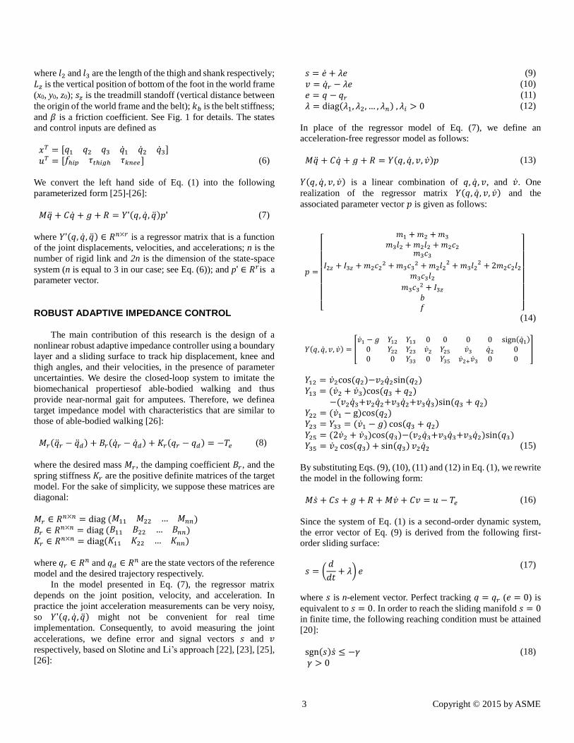
is discontinuous and causes control chattering, the saturation
function sat(𝑠/𝜑) (see Fig.2) promises to provide better
performance than the sign function. So we modify the control
law of Eq. (20) as follows:
𝑢 = �̂��̇� + �̂�𝑣 + �̂� + �̂� + �̂�𝑒 − 𝐾𝑑 sat(𝑠/𝜑) (21)
where 𝜑 is the width of the saturation function.
The control law of Eq. (21) comprises two different parts.
The first part, �̂��̇� + �̂�𝑣 + �̂� + �̂�, is an adaptive control term that
is responsible for handling the uncertain parameters. The second
part,�̂�𝑒 − 𝐾𝑑sat(𝑠/𝜑), is a robust control term that is responsible
for dealing with the condition of Eq. (18) and the variations of
the external inputs 𝑇𝑒. Substituting Eq. (21) into Eq. (16) and
defining �̃� = 𝑀 − �̂�, �̃� = 𝐶 − �̂� , �̃� = 𝑔 − �̂� , �̃� = 𝑅 − �̂�,
and 𝑝 = 𝑝 − �̂�, we derive the closed-loop system as follows:
𝑀�̇� + 𝐶𝑠 + 𝐾𝑑sat(𝑠/𝜑) + ( 𝑇𝑒 − �̂�𝑒) = −(�̃��̇� + �̃�𝑣 + �̃� + �̃�)
(22)
We can separate the right side of Eq. (22) into two different parts:
the regressor matrix 𝑌(𝑞, �̇�, 𝑣, �̇�) and the parameter estimation
error vector𝑝. Therefore, we can present Eq. (22) in the
following regressor (linear parametric) form:
𝑀�̇� + 𝐶𝑠 + 𝐾𝑑sat(𝑠/𝜑) + ( 𝑇𝑒 − �̂�𝑒) = −𝑌(𝑞, �̇�, 𝑣, �̇�)�̃� (23)
Next, to trade off control chattering and tracking accuracy, and
to create an adaptation dead zone to prevent unfavorable
parameter drift, we define a trajectory 𝑠∆ as follows [20]-[25]:
𝑠∆ = {0 , |𝑠| ≤ 𝜑
𝑠 − 𝜑 sat(𝑠/𝜑) , |𝑠| > 𝜑
(24)
where the region |𝑠| ≤ 𝜑 is the boundary layer; and 𝜑 is the
boundary layer thickness and the width of the saturation
function. We depict the trajectory 𝑠∆ and the function sat(𝑠/𝜑)
in Fig. 2.
Fig. 2. Saturation function and trajectory 𝒔∆
To drive a stable adaptation law based on the trajectory 𝑠∆,
we present a continuously differentiable scalar positive definite
Lyapunov function as follows [25]:
𝑉(𝑠∆, 𝑝) =1
2(𝑠∆
𝑇𝑀 𝑠∆) +1
2(𝑝𝑇𝜇 𝑝)
(25)
where 𝜇 is a design parameter such that 𝜇 =diag(𝜇1, 𝜇2, … , 𝜇𝑟) , with 𝜇𝑖 > 0. We find the derivative of the
Lyapunov function as follows:
�̇�(𝑠∆, 𝑝) =1
2(�̇�∆
𝑇𝑀 𝑠∆ + 𝑠∆𝑇𝑀 �̇�∆) +
1
2(𝑠∆
𝑇�̇�𝑠∆) +
1
2(�̇�𝑇𝜇 𝑝 + 𝑝𝑇𝜇 �̇�)
= 𝑠∆𝑇𝑀 �̇�∆ +
1
2(𝑠∆
𝑇�̇�𝑠∆) + �̇�𝑇𝜇 𝑝
Inside the boundary layer �̇�∆ = 0, and outside of it �̇�∆ = �̇�, so
�̇�(𝑠∆, 𝑝) = 𝑠∆𝑇(−𝐶𝑠 − 𝐾𝑑𝑠𝑎𝑡 (
𝑠
𝜑) + (�̂�𝑒 − 𝑇𝑒) −
𝑌(𝑞, �̇�, 𝑣, �̇�)𝑝) +1
2(𝑠∆
𝑇�̇�𝑠∆) + �̇�𝑇𝜇 𝑝
=1
2𝑠∆
𝑇(�̇� − 2𝐶)𝑠∆ − 𝑠∆𝑇 𝑌(𝑞, �̇�, 𝑣, �̇�)𝑝 −
𝑠∆𝑇𝐾𝑑sat(𝑠/𝜑) + 𝑠∆
𝑇(�̂�𝑒 − 𝑇𝑒) + �̇�𝑇𝜇 𝑝
Matrix �̇� − 2𝐶 is skew-symmetric, so 𝑠∆𝑇(�̇� − 2𝐶)𝑠∆ = 0.
Also, 𝑠∆𝑇sat(𝑠/𝜑) is equal to |𝑠∆
𝑇|, so we can simplify the
derivative as follows:
�̇�(𝑠∆, 𝑝) = −𝐾𝑑|𝑠∆| + 𝑠∆𝑇(�̂�𝑒 − 𝑇𝑒) +
�̇�𝑇𝜇 𝑝 − 𝑠∆𝑇𝑌(𝑞, �̇�, 𝑣, �̇�)𝑝
(26)
5 Copyright © 2015 by ASME
In order to ensure semi-negative definiteness for�̇�(𝑠∆, 𝑝),
we constrain the term �̇�𝑇𝜇 𝑝 − 𝑠∆𝑇𝑌(𝑞, �̇�, 𝑣, �̇�)𝑝 to zero in
Eq. (26), which allows us to derive a stable update law as
follows:
�̇̂� = −𝜇−1𝑌𝑇(𝑞, �̇�, 𝑣, �̇�)𝑠∆ (27)
By defining 𝐾𝑑𝑖= 𝐹 + 𝛾 for some n-element vectors F and 𝛾,
which comes from the inequality |�̂�𝑒 − 𝑇𝑒| ≤ 𝐹 (that is, the
difference between �̂�𝑒 and 𝑇𝑒 is bounded element-wise) and
from the inequality sgn(𝑠)�̇� ≤ −𝛾, we obtain the final form of
�̇�(𝑠∆, 𝑝) as follows:
�̇�(𝑠∆, 𝑝) ≤ −𝛾|𝑠∆| ≤ 0 (28)
It is seen that the derivative of the proposed Lyapunov
function is negative semi-definite, so we utilize Barbalat’s
lemma [25] to prove the asymptotic stability of the closed-loop
system.
Barbalat’s lemma: If a candidate Lyapunov function 𝑽 =𝑽(𝒕, 𝒙) satisfies the following conditions:
I. 𝑽(𝒕, 𝒙) is lower-bounded.
II. �̇�(𝒕, 𝒙) is negative semi-definite.
III. �̈�(𝒕, 𝒙) is bounded (�̇�(𝒕, 𝒙)is uniformly
continuous)
then �̇�(𝑡, 𝑥) → 0 as 𝑡 → ∞, which means that the closed-loop
system is asymptotically stable.
Theorem1: The tracking errors defined in Eq. (11)
asymptotically converge to zero, which in turn results in
asymptotically perfect tracking (𝑞 → 𝑞𝑟).
Proof: Items I and II in Barbalat’s lemma can easily be
shown from Eqs. (25) and (26) respectively. We thus conclude
that V is bounded; therefore, all terms in V in Eq. (25), namely,
𝑠∆ and 𝑝, are bounded. Since𝑝 is constant, �̂� is bounded, and
since𝑠∆ is bounded, 𝑠 is bounded. �̈�(𝑠∆, 𝑝) ≤ −𝛾�̇� and in the
worst case we have
�̈�(𝑠∆, 𝑝) = −𝛾�̇�
= −𝛾𝑀−1(−𝐶𝑠 − 𝐾𝑑sat(𝑠/𝜑) +
(�̂�𝑒 − 𝑇𝑒) − 𝑌(𝑞, �̇�, 𝑣, �̇�)𝑝)
(29)
Since the model and controller parameters (𝑀,𝐶, 𝑌, 𝛾, and
𝐾𝑑) are bounded, |�̂�𝑒 − 𝑇𝑒| ≤ 𝐹 and 𝑝 and 𝑠 are bounded, we
conclude that �̈� is bounded. Consequently, since we confirm
premises I, II, and III in Barbalat’s lemma, we conclude that
�̇�(𝑠∆, 𝑝) → 0 as 𝑡 → ∞. This implies that −𝛾|𝑠∆| in Eq. (28)
converges to 0, and we easily conclude that the inequality of
Eq. (28) can be written as �̇�(𝑠∆, 𝑝) = −𝛾|𝑠∆|. �̇�(𝑠∆, 𝑝) →0⟾𝛾|𝑠∆| → 0⟾ 𝑠 → 0 ⟾𝑒 and �̇� → 0 and eventually 𝑞
converges to 𝑞𝑟 to attain perfect tracking. ■
By using the Lyapunov function of Eq. (25), and the
adaptation law of Eq. (27), and by considering 𝐾𝑑𝑖> 𝐹, the
proposed system is asymptotically stable and the controller is
robust to the effects of GRF. The robust model reference adaptive
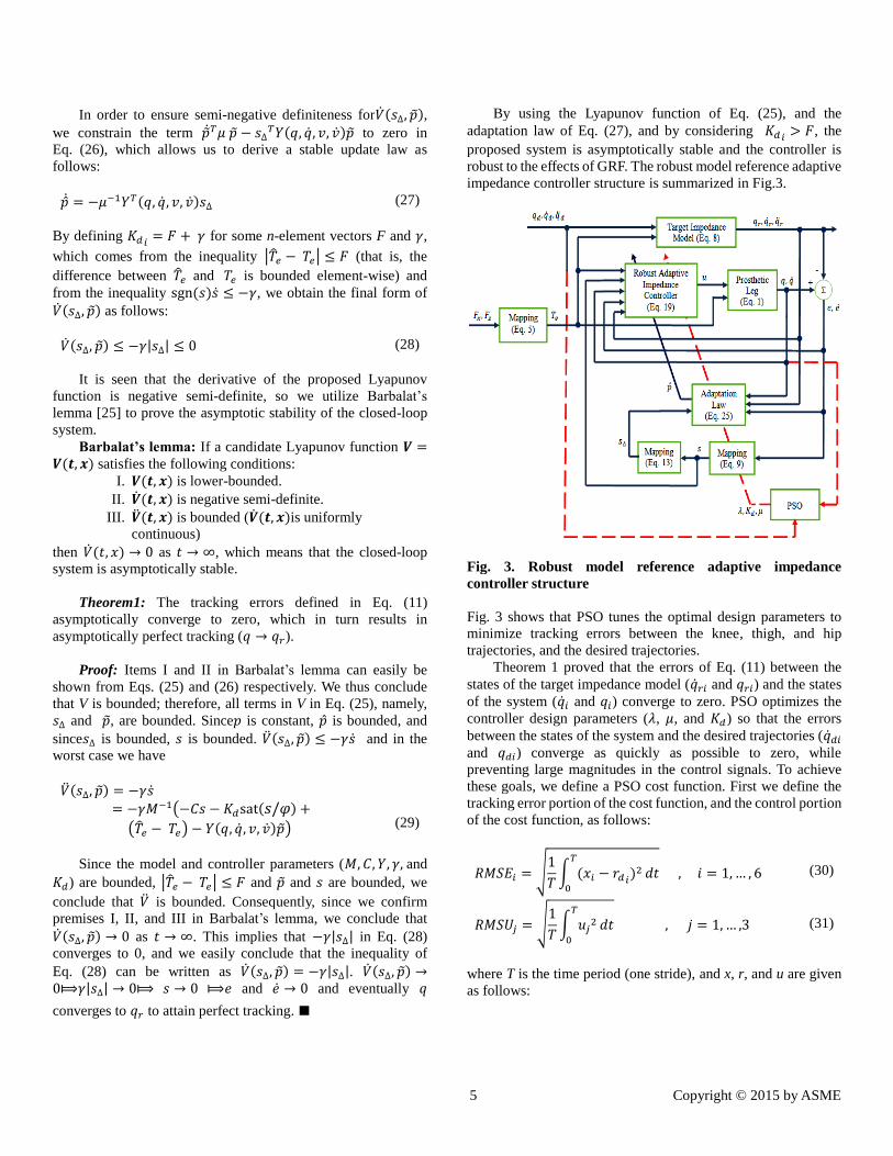
impedance controller structure is summarized in Fig.3.
Fig. 3. Robust model reference adaptive impedance
controller structure
Fig. 3 shows that PSO tunes the optimal design parameters to
minimize tracking errors between the knee, thigh, and hip
trajectories, and the desired trajectories.
Theorem 1 proved that the errors of Eq. (11) between the
states of the target impedance model (�̇�𝑟𝑖 and 𝑞𝑟𝑖) and the states
of the system (�̇�𝑖 and 𝑞𝑖) converge to zero. PSO optimizes the
controller design parameters (𝜆, 𝜇, and 𝐾𝑑) so that the errors
between the states of the system and the desired trajectories (�̇�𝑑𝑖
and 𝑞𝑑𝑖) converge as quickly as possible to zero, while
preventing large magnitudes in the control signals. To achieve
these goals, we define a PSO cost function. First we define the
tracking error portion of the cost function, and the control portion
of the cost function, as follows:
𝑅𝑀𝑆𝐸𝑖 = √1
𝑇∫ (𝑥𝑖 − 𝑟𝑑𝑖
)2 𝑑𝑡𝑇
0
, 𝑖 = 1, … , 6
(30)
𝑅𝑀𝑆𝑈𝑗 = √1
𝑇∫ 𝑢𝑗
2 𝑑𝑡𝑇
0
, 𝑗 = 1, … ,3
(31)
where T is the time period (one stride), and x, r, and u are given
as follows:
6 Copyright © 2015 by ASME
𝑥𝑇 = [𝑞1 𝑞2 𝑞3 �̇�1 �̇�2 �̇�3] 𝑟𝑇 = [𝑟𝑑1
𝑟𝑑2𝑟𝑑3
𝑟𝑑4𝑟𝑑5
𝑟𝑑6] = [𝑞𝑑1
𝑞𝑑2𝑞𝑑3
�̇�𝑑1�̇�𝑑2
�̇�𝑑3] 𝑢𝑇 = [𝑓ℎ𝑖𝑝 𝜏𝑡ℎ𝑖𝑔ℎ 𝜏𝑘𝑛𝑒𝑒]
(32)
We then define the normalized cost components as follows:
𝐶𝑜𝑠𝑡𝐸𝑖 =𝑅𝑀𝑆𝐸𝑖
maxt∈[0,T]
|𝑥𝑖 − 𝑟𝑑𝑖| 𝐶𝑜𝑠𝑡𝑈𝑗 =
𝑅𝑀𝑆𝑈𝑗
maxt∈[0,T]
|𝑢𝑗|
(33)
The total tracking cost, total control cost, and total combined cost
are finally given as follows.
𝐶𝑜𝑠𝑡𝐸 = ∑𝐶𝑜𝑠𝑡𝐸𝑖 ,
6
𝑖=1
𝐶𝑜𝑠𝑡𝑈 = ∑𝐶𝑜𝑠𝑡𝑈𝑖
3
𝑗=1
𝐶𝑜𝑠𝑡 = 𝐶𝑜𝑠𝑡𝐸 + 𝐶𝑜𝑠𝑡𝑈
(34)
The Cost variable in the previous equation is the objective
function of the PSO algorithm.
SIMULATION RESULTS
The desired trajectory in this paper is walking data obtained
by the Motion Studies Laboratory (MSL) of the Cleveland
Department of Veterans Affairs Medical Center (VAMC). In this
section we show the effectiveness of the proposed controller of
Fig. 3 by performing simulation studies on the prosthesis robot
model.
In the system model considered here, we have 𝑞 ∈ 𝑅3,
so𝑀𝑟 = diag(𝑀11 𝑀22 𝑀33), 𝐵𝑟 = diag(𝐵11 𝐵22 𝐵33),
and 𝐾𝑟 = diag(𝐾11 𝐾22 𝐾33). To have two equal real roots
for each of joint displacements (critically damped responses for
the hip vertical displacement 𝑞1, and the thigh and knee angles
𝑞2and 𝑞3) in the target impedance model of Eq. (8), 𝐵𝑖𝑖must be
equal to 2√𝐾𝑖𝑖𝑀𝑖𝑖 and the two roots can be calculated
as−√𝐾𝑖𝑖/𝑀𝑖𝑖. To have two different real roots, 𝐵𝑖𝑖must be
greater than 2√𝐾𝑖𝑖𝑀𝑖𝑖. We define the target impedance model
with two real roots at−27and −72 for both the knee and thigh,
and two real roots at −52 and −947 for the hip displacement. We
choose these values heuristically so that the target impedance
model is stable, behaves similarly to an able-bodied leg, and
gives near-perfect tracking. This approach results in the
following impedance model matrices:
𝑀𝑟 = diag (10 10 10)
𝐾𝑟 = diag (500000 20000 20000)
𝐵𝑟 = diag (10000 1000 1000)
Particle Swarm Optimization
We use PSO to tune the controller and estimator parameters [27].
We use the following parameters for PSO: optimization problem
dimension=14, number of iterations=20, population size=72,
maximum rates for cognition and social learning=2.05, damping
ratio for inertia rate=0.9, and scale factor=0.1.
We consider the following values for the minimum and
maximum values of the search domain of 𝜇, 𝐾𝑑, and 𝜆:
𝜇𝑖 ∈ [0.001, 0.01] , 𝑖 = 1, … , 8
𝐾𝑑𝑖∈ [50, 150] , 𝑖 = 1, … , 3
𝜆𝑖 ∈ [50, 150] , 𝑖 = 1, … ,3
where we use 𝜇 in Eqs. (9) and (10) to build the signal and error
vectors, 𝐾𝑑 in Eq. (20) to design the controller, and 𝜆in Eq. (27)
to design the update law. After some trial and error, we find good
performance with a boundary layer thicknesses for the
trajectories 𝑠∆(shown in Fig.2) for all joint displacements as𝜑1 =𝜑2 = 𝜑3 = 0.5. The initial state of the system is given as
follows:
𝑥0𝑇 = [0.019 1.13 0.09 0.09 0 1.6].
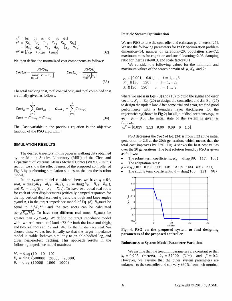
PSO decreases the 𝐶𝑜𝑠𝑡 of Eq. (34) is from 3.33 at the initial
generation to 2.6 at the 20th generation, which means that the
total cost improves by 22%. Fig. 4 shows the best cost values
over the 20 generations. The best solution found by PSO is given
as follows:
The robust term coefficients: 𝐾𝑑 = diag(89, 117, 103)
The adaptation rates: 𝜇 = diag(0.013 0.010 0.011 0.015 0.015 0.014 0.019 0.01)
The sliding term coefficients: 𝜆 = diag(105, 121, 98)
Fig. 4. PSO on the proposed system to find designing
parameters of the proposed controller
Robustness to System Model Parameter Variations
We assume that the treadmill parameters are constant so that
𝑠𝑧 = 0.905 (meters), 𝑘𝑏 = 37000 (N/m), and 𝛽 = 0.2.
However, we assume that the other system parameters are
unknown to the controller and can vary ±30% from their nominal
0 5 10 15 202.55
2.7
2.85
3
3.15
3.3
3.45
3.6
Iteration
Best C
ost
7 Copyright © 2015 by ASME
values. We list the nominal values of the system parameters in
Table I.
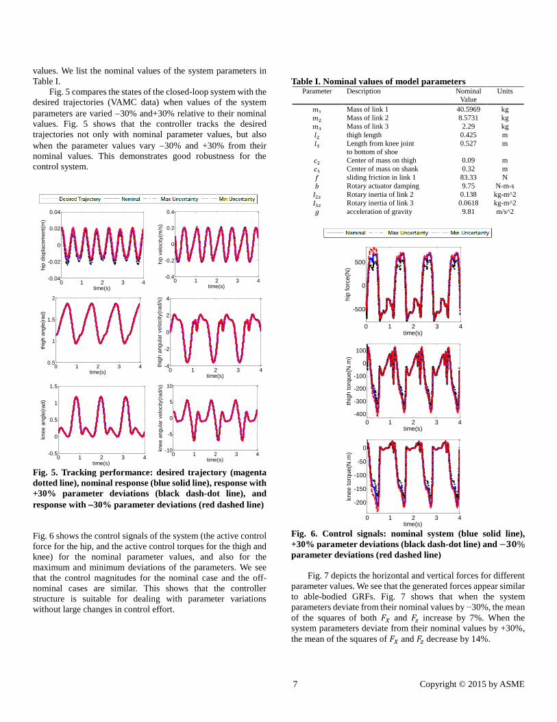
Fig. 5 compares the states of the closed-loop system with the
desired trajectories (VAMC data) when values of the system
parameters are varied 30% and+30% relative to their nominal
values. Fig. 5 shows that the controller tracks the desired
trajectories not only with nominal parameter values, but also
when the parameter values vary 30% and +30% from their
nominal values. This demonstrates good robustness for the
control system.
Fig. 5. Tracking performance: desired trajectory (magenta
dotted line), nominal response (blue solid line), response with
+30% parameter deviations (black dash-dot line), and
response with 30% parameter deviations (red dashed line)
Fig. 6 shows the control signals of the system (the active control
force for the hip, and the active control torques for the thigh and
knee) for the nominal parameter values, and also for the
maximum and minimum deviations of the parameters. We see
that the control magnitudes for the nominal case and the off-
nominal cases are similar. This shows that the controller
structure is suitable for dealing with parameter variations
without large changes in control effort.
Table I. Nominal values of model parameters Parameter Description Nominal
Value Units
𝑚1 Mass of link 1 40.5969 kg
𝑚2 Mass of link 2 8.5731 kg
𝑚3 Mass of link 3 2.29 kg
𝑙2 thigh length 0.425 m
𝑙3 Length from knee joint
to bottom of shoe
0.527 m
𝑐2 Center of mass on thigh 0.09 m
𝑐3 Center of mass on shank 0.32 m
𝑓 sliding friction in link 1 83.33 N
𝑏 Rotary actuator damping 9.75 N-m-s
𝐼2𝑧 Rotary inertia of link 2 0.138 kg-m^2
𝐼3𝑧 Rotary inertia of link 3 0.0618 kg-m^2
𝑔 acceleration of gravity 9.81 m/s^2
Fig. 6. Control signals: nominal system (blue solid line),
+30% parameter deviations (black dash-dot line) and −𝟑𝟎%
parameter deviations (red dashed line)
Fig. 7 depicts the horizontal and vertical forces for different
parameter values. We see that the generated forces appear similar
to able-bodied GRFs. Fig. 7 shows that when the system
parameters deviate from their nominal values by −30%, the mean
of the squares of both 𝐹𝑋 and 𝐹𝑧 increase by 7%. When the
system parameters deviate from their nominal values by +30%,
the mean of the squares of 𝐹𝑋 and 𝐹𝑧 decrease by 14%.
0 1 2 3 4-0.04
-0.02
0
0.02
0.04
time(s)
hip
dis
pla
cem
ent(
m)
0 1 2 3 4-0.4
-0.2
0
0.2
0.4
time(s)
hip
velo
city(m
/s)
0 1 2 3 40.5
1
1.5
2
time(s)
thig
h a
ngle
(ra
d)
0 1 2 3 4-4
-2
0
2
4
time(s)
thig
h a
ngula
r velo
city(r
ad/s
)
0 1 2 3 4-0.5
0
0.5
1
1.5
time(s)
knee a
ngle
(rad)
0 1 2 3 4-10
-5
0
5
10
time(s)
knee a
ngula
r ve
locity(r
ad
/s)
0 1 2 3 4
-500
0
500
time(s)
hip
fo
rce
(N)
0 1 2 3 4
-400
-300
-200
-100
0
100
time(s)
thig
h t
orq
ue(N
.m)
0 1 2 3 4
-200
-150
-100
-50
0
time(s)
knee t
orq
ue(N
.m)
8 Copyright © 2015 by ASME
Fig. 7. The horizontal and vertical forces (GRFs) for nominal
parameter values (blue solid line), +30% parameter
deviations (black dash-dot line) and 30% parameter
deviations (red dashed line). The heel strikes are shown in the
right subplot with circles on the x-axis
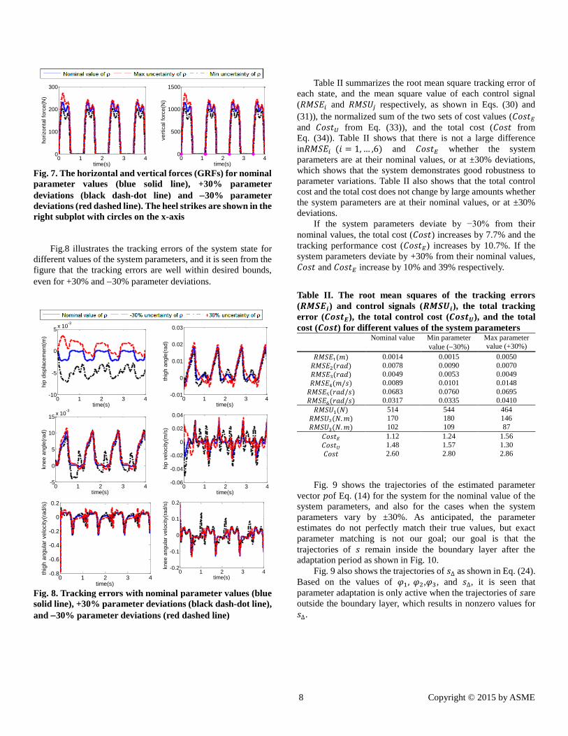
Fig.8 illustrates the tracking errors of the system state for
different values of the system parameters, and it is seen from the
figure that the tracking errors are well within desired bounds,
even for +30% and 30% parameter deviations.
Fig. 8. Tracking errors with nominal parameter values (blue
solid line), +30% parameter deviations (black dash-dot line),
and 30% parameter deviations (red dashed line)
Table II summarizes the root mean square tracking error of
each state, and the mean square value of each control signal
(𝑅𝑀𝑆𝐸𝑖 and 𝑅𝑀𝑆𝑈𝑗 respectively, as shown in Eqs. (30) and
(31)), the normalized sum of the two sets of cost values (𝐶𝑜𝑠𝑡𝐸
and 𝐶𝑜𝑠𝑡𝑈 from Eq. (33)), and the total cost (𝐶𝑜𝑠𝑡 from
Eq. (34)). Table II shows that there is not a large difference
in𝑅𝑀𝑆𝐸𝑖 (𝑖 = 1,… ,6) and 𝐶𝑜𝑠𝑡𝐸 whether the system
parameters are at their nominal values, or at ±30% deviations,
which shows that the system demonstrates good robustness to
parameter variations. Table II also shows that the total control
cost and the total cost does not change by large amounts whether
the system parameters are at their nominal values, or at ±30%
deviations.
If the system parameters deviate by −30% from their
nominal values, the total cost (𝐶𝑜𝑠𝑡) increases by 7.7% and the
tracking performance cost (𝐶𝑜𝑠𝑡𝐸) increases by 10.7%. If the
system parameters deviate by +30% from their nominal values,
𝐶𝑜𝑠𝑡 and 𝐶𝑜𝑠𝑡𝐸 increase by 10% and 39% respectively.
Table II. The root mean squares of the tracking errors
(𝑹𝑴𝑺𝑬𝒊) and control signals (𝑹𝑴𝑺𝑼𝒊), the total tracking
error (𝑪𝒐𝒔𝒕𝑬), the total control cost (𝑪𝒐𝒔𝒕𝑼), and the total
cost (𝑪𝒐𝒔𝒕) for different values of the system parameters Nominal value Min parameter
value (30%)
Max parameter
value (+30%)
𝑅𝑀𝑆𝐸1(𝑚) 0.0014 0.0015 0.0050
𝑅𝑀𝑆𝐸2(𝑟𝑎𝑑) 0.0078 0.0090 0.0070
𝑅𝑀𝑆𝐸3(𝑟𝑎𝑑) 0.0049 0.0053 0.0049
𝑅𝑀𝑆𝐸4(𝑚/𝑠) 0.0089 0.0101 0.0148
𝑅𝑀𝑆𝐸5(𝑟𝑎𝑑/𝑠) 0.0683 0.0760 0.0695
𝑅𝑀𝑆𝐸6(𝑟𝑎𝑑/𝑠) 0.0317 0.0335 0.0410
𝑅𝑀𝑆𝑈1(𝑁) 514 544 464
𝑅𝑀𝑆𝑈2(𝑁.𝑚) 170 180 146
𝑅𝑀𝑆𝑈3(𝑁.𝑚) 102 109 87
𝐶𝑜𝑠𝑡𝐸 1.12 1.24 1.56
𝐶𝑜𝑠𝑡𝑈 1.48 1.57 1.30
𝐶𝑜𝑠𝑡 2.60 2.80 2.86
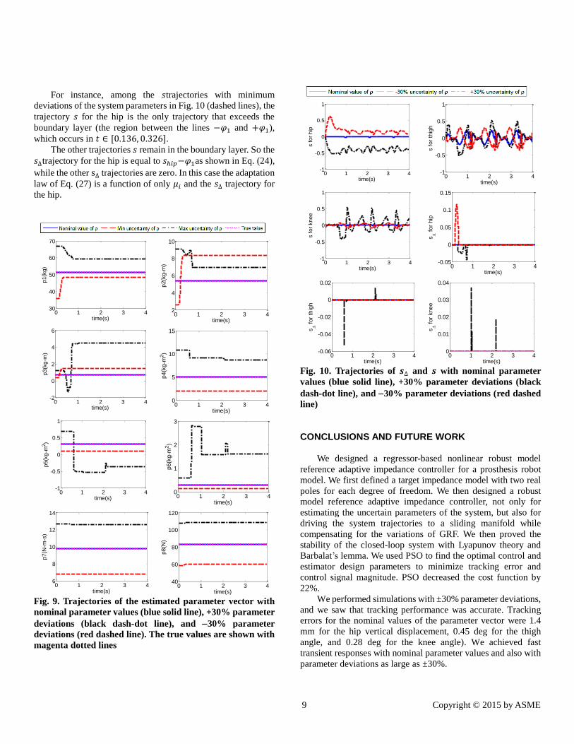
Fig. 9 shows the trajectories of the estimated parameter
vector 𝑝of Eq. (14) for the system for the nominal value of the
system parameters, and also for the cases when the system
parameters vary by ±30%. As anticipated, the parameter
estimates do not perfectly match their true values, but exact
parameter matching is not our goal; our goal is that the
trajectories of 𝑠 remain inside the boundary layer after the
adaptation period as shown in Fig. 10.
Fig. 9 also shows the trajectories of 𝑠∆ as shown in Eq. (24).
Based on the values of 𝜑1, 𝜑2,𝜑3, and 𝑠∆, it is seen that
parameter adaptation is only active when the trajectories of 𝑠are
outside the boundary layer, which results in nonzero values for
𝑠∆.
0 1 2 3 40
100
200
300
time(s)
horizonta
l fo
rce(N
)
0 1 2 3 40
500
1000
1500
time(s)ve
rtic
al fo
rce
(N)
0 1 2 3 4-10
-5
0
5x 10
-3
time(s)
hip
dis
pla
ce
me
nt(
m)
0 1 2 3 4-0.01
0
0.01
0.02
0.03
time(s)
thig
h a
ngle
(rad)
0 1 2 3 4-5
0
5
10
15x 10
-3
time(s)
knee a
ngle
(rad)
0 1 2 3 4-0.06
-0.04
-0.02
0
0.02
0.04
time(s)
hip
ve
locity(m
/s)
0 1 2 3 4-0.8
-0.6
-0.4
-0.2
0
0.2
time(s)
thig
h a
ngu
lar
ve
locity(r
ad
/s)
0 1 2 3 4-0.2
-0.1
0
0.1
0.2
time(s)
knee a
ngula
r velo
city(r
ad/s
)
9 Copyright © 2015 by ASME
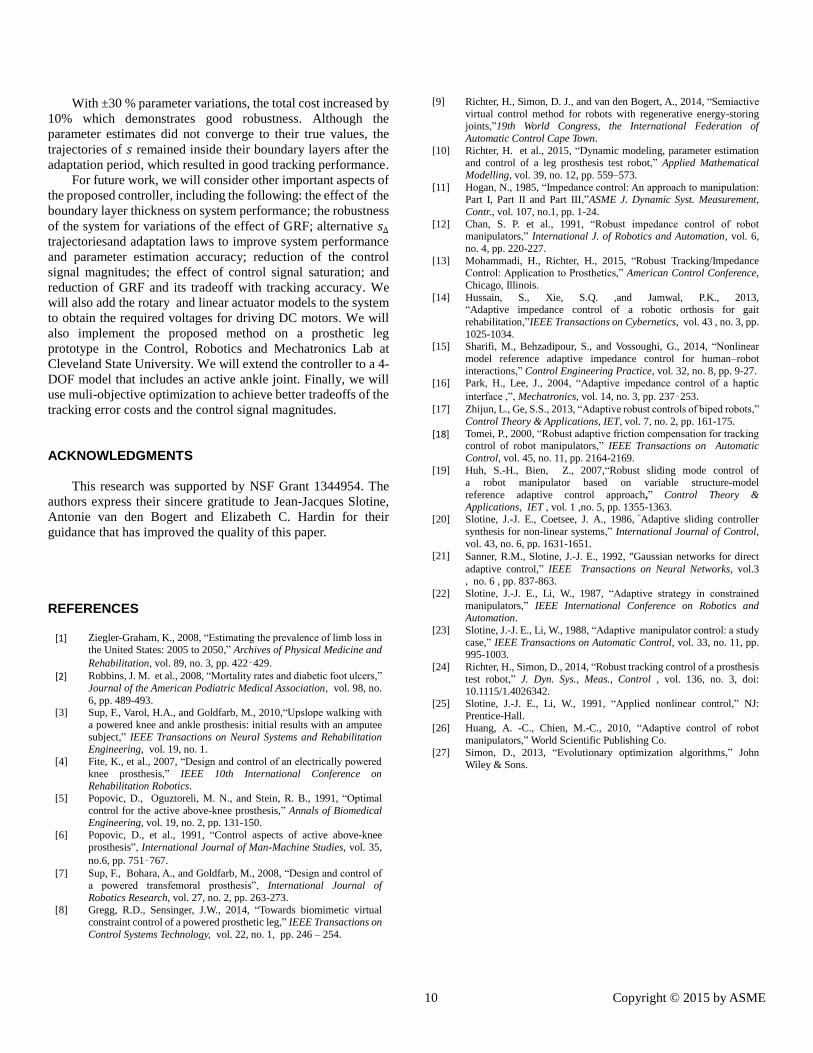
For instance, among the 𝑠trajectories with minimum
deviations of the system parameters in Fig. 10 (dashed lines), the
trajectory 𝑠 for the hip is the only trajectory that exceeds the
boundary layer (the region between the lines −𝜑1 and +𝜑1),
which occurs in 𝑡 ∈ [0.136, 0.326]. The other trajectories 𝑠 remain in the boundary layer. So the
𝑠∆trajectory for the hip is equal to 𝑠ℎ𝑖𝑝−𝜑1as shown in Eq. (24),
while the other s∆ trajectories are zero. In this case the adaptation
law of Eq. (27) is a function of only 𝜇𝑖 and the 𝑠∆ trajectory for
the hip.
Fig. 9. Trajectories of the estimated parameter vector with
nominal parameter values (blue solid line), +30% parameter
deviations (black dash-dot line), and 30% parameter
deviations (red dashed line). The true values are shown with
magenta dotted lines
Fig. 10. Trajectories of 𝒔∆ and 𝒔 with nominal parameter
values (blue solid line), +30% parameter deviations (black
dash-dot line), and 30% parameter deviations (red dashed
line)
CONCLUSIONS AND FUTURE WORK
We designed a regressor-based nonlinear robust model
reference adaptive impedance controller for a prosthesis robot
model. We first defined a target impedance model with two real
poles for each degree of freedom. We then designed a robust
model reference adaptive impedance controller, not only for
estimating the uncertain parameters of the system, but also for
driving the system trajectories to a sliding manifold while
compensating for the variations of GRF. We then proved the
stability of the closed-loop system with Lyapunov theory and
Barbalat’s lemma. We used PSO to find the optimal control and
estimator design parameters to minimize tracking error and
control signal magnitude. PSO decreased the cost function by
22%.
We performed simulations with ±30% parameter deviations,
and we saw that tracking performance was accurate. Tracking
errors for the nominal values of the parameter vector were 1.4
mm for the hip vertical displacement, 0.45 deg for the thigh
angle, and 0.28 deg for the knee angle). We achieved fast
transient responses with nominal parameter values and also with
parameter deviations as large as ±30%.
0 1 2 3 430
40
50
60
70
p1(k
g)
time(s)0 1 2 3 4
2
4
6
8
10
p2
(kg
-m)
time(s)
0 1 2 3 4-2
0
2
4
6
p3(k
g-m
)
time(s)0 1 2 3 4
0
5
10
15
p4(k
g-m
2)
time(s)
0 1 2 3 4-1
-0.5
0
0.5
1
p5(k
g-m
2)
time(s) 0 1 2 3 40
1
2
3
p6(k
g-m
2)
time(s)
0 1 2 3 46
8
10
12
14
p7
(N-m
-s)
time(s)0 1 2 3 4
40
60
80
100
120
p8(N
)
time(s)
0 1 2 3 4-1
-0.5
0
0.5
1
time(s)
s f
or
hip
0 1 2 3 4-1
-0.5
0
0.5
1
time(s)
s f
or
thig
h
0 1 2 3 4-1
-0.5
0
0.5
1
time(s)
s f
or
kn
ee
0 1 2 3 4-0.05
0
0.05
0.1
0.15
time(s)
s f
or
hip
0 1 2 3 4-0.06
-0.04
-0.02
0
0.02
time(s)
s f
or
thig
h
0 1 2 3 40
0.01
0.02
0.03
0.04
time(s)
s f
or
kn
ee
10 Copyright © 2015 by ASME
With ±30 % parameter variations, the total cost increased by
10% which demonstrates good robustness. Although the
parameter estimates did not converge to their true values, the
trajectories of 𝑠 remained inside their boundary layers after the
adaptation period, which resulted in good tracking performance.
For future work, we will consider other important aspects of
the proposed controller, including the following: the effect of the
boundary layer thickness on system performance; the robustness
of the system for variations of the effect of GRF; alternative 𝑠∆
trajectoriesand adaptation laws to improve system performance
and parameter estimation accuracy; reduction of the control
signal magnitudes; the effect of control signal saturation; and
reduction of GRF and its tradeoff with tracking accuracy. We
will also add the rotary and linear actuator models to the system
to obtain the required voltages for driving DC motors. We will
also implement the proposed method on a prosthetic leg
prototype in the Control, Robotics and Mechatronics Lab at
Cleveland State University. We will extend the controller to a 4-
DOF model that includes an active ankle joint. Finally, we will
use muli-objective optimization to achieve better tradeoffs of the
tracking error costs and the control signal magnitudes.
ACKNOWLEDGMENTS
This research was supported by NSF Grant 1344954. The
authors express their sincere gratitude to Jean-Jacques Slotine,
Antonie van den Bogert and Elizabeth C. Hardin for their
guidance that has improved the quality of this paper.
REFERENCES
[1] Ziegler-Graham, K., 2008, “Estimating the prevalence of limb loss in the United States: 2005 to 2050,” Archives of Physical Medicine and
Rehabilitation, vol. 89, no. 3, pp. 422–429.
[2] Robbins, J. M. et al., 2008, “Mortality rates and diabetic foot ulcers,”
Journal of the American Podiatric Medical Association, vol. 98, no.
6, pp. 489-493. [3] Sup, F., Varol, H.A., and Goldfarb, M., 2010,“Upslope walking with
a powered knee and ankle prosthesis: initial results with an amputee
subject,” IEEE Transactions on Neural Systems and Rehabilitation Engineering, vol. 19, no. 1.
[4] Fite, K., et al., 2007, “Design and control of an electrically powered
knee prosthesis,” IEEE 10th International Conference on
Rehabilitation Robotics.
[5] Popovic, D., Oguztoreli, M. N., and Stein, R. B., 1991, “Optimal
control for the active above-knee prosthesis,” Annals of Biomedical Engineering, vol. 19, no. 2, pp. 131-150.
[6] Popovic, D., et al., 1991, “Control aspects of active above-knee
prosthesis”, International Journal of Man-Machine Studies, vol. 35,
no.6, pp. 751–767.
[7] Sup, F., Bohara, A., and Goldfarb, M., 2008, “Design and control of a powered transfemoral prosthesis”, International Journal of
Robotics Research, vol. 27, no. 2, pp. 263-273.
[8] Gregg, R.D., Sensinger, J.W., 2014, “Towards biomimetic virtual constraint control of a powered prosthetic leg,” IEEE Transactions on
Control Systems Technology, vol. 22, no. 1, pp. 246 – 254.
[9] Richter, H., Simon, D. J., and van den Bogert, A., 2014, “Semiactive
virtual control method for robots with regenerative energy-storing joints,”19th World Congress, the International Federation of
Automatic Control Cape Town.
[10] Richter, H. et al., 2015, “Dynamic modeling, parameter estimation and control of a leg prosthesis test robot,” Applied Mathematical
Modelling, vol. 39, no. 12, pp. 559–573.
[11] Hogan, N., 1985, “Impedance control: An approach to manipulation: Part I, Part II and Part III,”ASME J. Dynamic Syst. Measurement,
Contr., vol. 107, no.1, pp. 1-24.
[12] Chan, S. P. et al., 1991, “Robust impedance control of robot manipulators,” International J. of Robotics and Automation, vol. 6,
no. 4, pp. 220-227.
[13] Mohammadi, H., Richter, H., 2015, “Robust Tracking/Impedance Control: Application to Prosthetics,” American Control Conference,
Chicago, Illinois.
[14] Hussain, S., Xie, S.Q. ,and Jamwal, P.K., 2013, “Adaptive impedance control of a robotic orthosis for gait
rehabilitation,”IEEE Transactions on Cybernetics, vol. 43 , no. 3, pp.
1025-1034. [15] Sharifi, M., Behzadipour, S., and Vossoughi, G., 2014, “Nonlinear
model reference adaptive impedance control for human–robot
interactions,” Control Engineering Practice, vol. 32, no. 8, pp. 9-27. [16] Park, H., Lee, J., 2004, “Adaptive impedance control of a haptic
interface ,”, Mechatronics, vol. 14, no. 3, pp. 237–253.
[17] Zhijun, L., Ge, S.S., 2013, “Adaptive robust controls of biped robots,”
Control Theory & Applications, IET, vol. 7, no. 2, pp. 161-175.
[18] Tomei, P., 2000, “Robust adaptive friction compensation for tracking control of robot manipulators,” IEEE Transactions on Automatic
Control, vol. 45, no. 11, pp. 2164-2169.
[19] Huh, S.-H., Bien, Z., 2007,“Robust sliding mode control of a robot manipulator based on variable structure-model
reference adaptive control approach,” Control Theory &
Applications, IET , vol. 1 ,no. 5, pp. 1355-1363. [20] Slotine, J.-J. E., Coetsee, J. A., 1986, “Adaptive sliding controller
synthesis for non-linear systems,” International Journal of Control,
vol. 43, no. 6, pp. 1631-1651.
[21] Sanner, R.M., Slotine, J.-J. E., 1992, “Gaussian networks for direct
adaptive control,” IEEE Transactions on Neural Networks, vol.3 , no. 6 , pp. 837-863.
[22] Slotine, J.-J. E., Li, W., 1987, “Adaptive strategy in constrained
manipulators,” IEEE International Conference on Robotics and Automation.
[23] Slotine, J.-J. E., Li, W., 1988, “Adaptive manipulator control: a study
case,” IEEE Transactions on Automatic Control, vol. 33, no. 11, pp. 995-1003.
[24] Richter, H., Simon, D., 2014, “Robust tracking control of a prosthesis
test robot,” J. Dyn. Sys., Meas., Control , vol. 136, no. 3, doi: 10.1115/1.4026342.
[25] Slotine, J.-J. E., Li, W., 1991, “Applied nonlinear control,” NJ:
Prentice-Hall. [26] Huang, A. -C., Chien, M.-C., 2010, “Adaptive control of robot
manipulators,” World Scientific Publishing Co.
[27] Simon, D., 2013, “Evolutionary optimization algorithms,” John Wiley & Sons.


![ROBUST ADAPTIVE BEAMFORMER WITH · PDF filebust adaptive beamforming, ... strained adaptive beamformer is studied in [5, 6] and widely used thereafter. Recently some interesting robust](https://img.pdfslide.net/doc/110x75/5ab383fc7f8b9ad9788e2684/robust-adaptive-beamformer-with-adaptive-beamforming-strained-adaptive.jpg)