Embed Size (px)
Citation preview
CORONADO SYSTEMS, BENOIT BOULET REV. 0 , JULY 2000WITH N. AOUF
5REXVW�,QGXVWULDO�&RQWURO
Course Notes
Part 2: Robust and Optimal Control
ROBUST INDUSTRIAL CONTROL
NORMS - 2/117
1 NORMS OF SIGNALS AND SYSTEMS 4
1.1 Vector and matrix norms 4
1.2 L2-norm for finite-energy signals 5
1.3 Power "norm" for finite-power signals 6
1.4 L2 norm of LTI systems and the space H2 of stable causal systems 71.4.1 How to compute the 2$ -norm of stable systems 9
1.5 L∞ norm of LTI systems and the space H∞ of stable systems 91.5.1 How to compute the ∞$ -norm of stable systems 10
1.6 Relationships between input and output signal norms and system norms 10
2 H2 OPTIMAL CONTROL 11
2.1 Algebraic Riccati Equations 11
2.2 Problem setup 13
2.3 IMC H2-optimal LTI controller 192.3.1 Minimum-phase plants 242.3.2 Non-minimum-phase plants 25
3 H∞ OPTIMAL CONTROL 29
3.1 Problem setup 29
3.2 Solution to simplified suboptimal ∞ problem 31
4 UNCERTAINTY MODELING FOR ROBUST CONTROL 36
4.1 Unstructured uncertainty 364.1.1 Additive uncertainty model 364.1.2 Output multiplicative uncertainty 374.1.3 Input multiplicative uncertainty 394.1.4 Input inverse multiplicative uncertainty 404.1.5 Output inverse multiplicative uncertainty 404.1.6 Feedback uncertainty 414.1.7 Linear fractional uncertainty 414.1.8 Representing uncertainty in the frequency domain 43
4.2 Theorems for robust closed-loop stability with unstructured uncertainty 454.2.1 Robust stability with additive uncertainty 484.2.2 Robust stability with multiplicative uncertainty 504.2.3 Robust stability with inverse multiplicative uncertainty 524.2.4 Robust stability with feedback uncertainty 53

ROBUST INDUSTRIAL CONTROL
NORMS - 3/117
4.2.5 Robust stability with linear fractional uncertainty 54
4.3 Structured uncertainty 60
4.4 Robust closed-loop stability with structured uncertainty: µ -Analysis 644.4.1 The structured singular value 644.4.2 Well-posedness and the main loop theorem 694.4.3 Robust stability with structured uncertainty 714.4.4 Robust performance with structured uncertainty 74
5 ROBUST H∞ CONTROL DESIGN 80
5.1 Objective 80
5.2 Mixed-sensitivity robust H∞ controller design 84
6 CONTROLLER DESIGN VIA MU-SYNTHESIS 86
7 ACRONYMS 95
8 REFERENCES 96
9 APPENDIX: MATLAB M-FILES 97

ROBUST INDUSTRIAL CONTROL
NORMS - 4/117
� 1RUPV RI VLJQDOV DQG V\VWHPV
Norms of signals and systems are used to quantify the performance and robustness of a controlsystem. They are used in robust optimal control theory.
��� 9HFWRU DQGPDWUL[ QRUPV
In finite-dimensional vector spaces, it is convenient to define norms to measure the length of vectors,and matrix norms to measure the maximum "gain" of the matrix.
The 2-norm (or Euclidean norm) of an n -dimensional complex vector nx∈� is defined as:
( )
( )
1
22
12 2 2 2
1 2 n
x x x
x x x
∗=
= + + +"(0.1)
where x∗ denotes the conjugate transpose of x . The spectral norm of an n m× complex matrixn mQ ×∈� is defined as its maximum singular value maxσ :
( ) ( )1
2max maxQ Q Q Qσ λ ∗ = = , (0.2)
where maxλ denotes the maximum eigenvalue. This matrix norm represents the maximum input-output
gain in terms of 2-norms of input and output vectors. One can show that, with mx∈� :
2 2
2
2 20 1 12
max max maxx x x
QxQ Qx Qx
x≠ ≤ == = = (0.3)
Example
Consider the complex linear matrix equation y Qx= where
1 31
2 21 2
jQ
+ − =
. (0.4)
The spectral norm of the matrix is given by:

ROBUST INDUSTRIAL CONTROL
NORMS - 5/117
( ) ( )1
2max max
1
2
max
1
2
max
1 3 1 31 1
2 2 2 21 2 1 2
3 32
2 2 5.79 2.413 3
52 2
Q Q Q Q
j j
j
j
σ λ
λ
λ
∗ = =
− + − = −
+
= = = −
(0.5)
Thus the maximum amplification from the 2-norm of the input vector to the 2-norm of the output vector
will be a gain of 2.41. If we randomly select an input vector, say 1
3
jx
+ =
for which
[ ]1
2
2
11 3 2 9 3.317
3
jx j
+ = − = + =
, then the output vector is
1 3 5 3 1 3112 2 2 2
31 2 7
jj jy
j
+ ++ + − − + = = +
(0.6)
and its 2-norm is computed to be 2
7.712y = . The gain produced by the matrix is thus
2
2
7.7122.325
3.317
y
x= = which is smaller than its norm 2.41Q = as expected.
��� /��QRUP IRU ILQLWH�HQHUJ\ VLJQDOV
The 2$ -norm (or 2-norm) of a signal ( )x t is the square root of its total energy over -∞ < t < ∞ and is
defined as:
( )1
22
2| ( ) |x x t dt
∞
−∞= ∫ (0.7)
The set of all finite-energy signals is called the space 2$ :
{ }2 2: :x x= < +∞$ (0.8)

ROBUST INDUSTRIAL CONTROL
NORMS - 6/117
A "large" signal would have a large 2$ -norm, hence it is a measure of the size of a signal. In a servo
system, the objective is to minimize the tracking error signal ( ) ( ) ( )de t y t y t= − . It makes sense to
try to minimize its 2$ -norm 2
e if the reference signal ( )dy t belongs to 2$ .
The following result allows us to compute the 2$ -norm in the frequency domain using the Fourier
transform ˆ( )x jω of the signal.
Parseval's Theorem
2 2 2
2
1ˆ( ) ( )
2x x t dt x j dω ω
π∞ ∞
−∞ −∞= =∫ ∫ . (0.9)
��� 3RZHU �QRUP� IRU ILQLWH�SRZHU VLJQDOV
The power "norm" of a signal ( )x t is the square root of its total average power over -∞ < t < ∞ and is
defined as:
1
221( ) : lim | ( ) |
2
T
TTpow x x t dt
T −→+∞
= ∫ . (0.10)
Note that for periodic signals, it is sufficient to compute the average power over one period only:
1
22
0
1( ) : | ( ) | , periodic of period
Tpow x x t dt x T
T = ∫ . (0.11)
Strictly speaking, the function ( )pow x is not a norm because it can be equal to 0 for nonzero signals,
e.g., for signals in 2$ . Apart from that, it behaves like a regular norm. For instance, the triangle
inequality holds:
( ) ( ) ( )pow x y pow x pow y+ ≤ + . (0.12)
The set ( of all finite-power signals is defined as follows:
{ }: : ( )x pow x= < +∞( (0.13)
Examples: ( ) 4x t = has infinite energy but a power norm of 4 (and a power of 16):
112 2221 4
( ) lim 4 lim 2 42 2
T
TT Tpow x dt T
T T−→∞ →∞
= = = ∫ . (0.14)
ROBUST INDUSTRIAL CONTROL
NORMS - 7/117
For a periodic complex exponential x t Cej t( ) = ω of period 2
Tπ
ω= :
112 222
0 0
1 | |( ) | | | |
T Tj t C
pow x Ce dt dt CT T
ω = = = ∫ ∫ (0.15)
Note that ej tω 0 has total average power and power norm equal to 1.
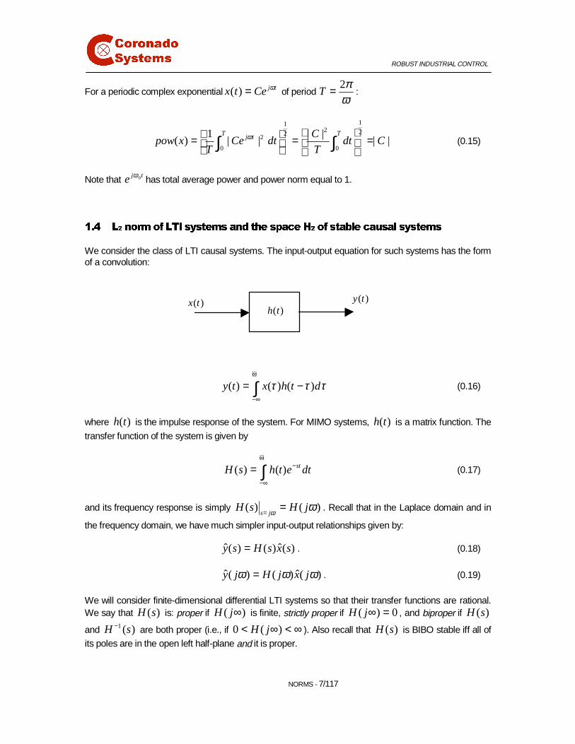
��� /�QRUPRI /7, V\VWHPVDQG WKH VSDFH+�RI VWDEOH FDXVDO V\VWHPV
We consider the class of LTI causal systems. The input-output equation for such systems has the formof a convolution:
( ) ( ) ( )y t x h t dτ τ τ+∞
−∞
= −∫ (0.16)
where ( )h t is the impulse response of the system. For MIMO systems, ( )h t is a matrix function. The
transfer function of the system is given by
( ) ( ) stH s h t e dt+∞
−
−∞
= ∫ (0.17)
and its frequency response is simply ( ) ( )s j
H s H jω
ω=
= . Recall that in the Laplace domain and in
the frequency domain, we have much simpler input-output relationships given by:
ˆ ˆ( ) ( ) ( )y s H s x s= . (0.18)
ˆ ˆ( ) ( ) ( )y j H j x jω ω ω= . (0.19)
We will consider finite-dimensional differential LTI systems so that their transfer functions are rational.We say that ( )H s is: proper if ( )H j∞ is finite, strictly proper if ( ) 0H j∞ = , and biproper if ( )H s
and 1( )H s− are both proper (i.e., if 0 ( )H j< ∞ < ∞ ). Also recall that ( )H s is BIBO stable iff all of
its poles are in the open left half-plane and it is proper.
( )x t ( )y t( )h t

ROBUST INDUSTRIAL CONTROL
NORMS - 8/117
The 2$ -norm (or 2-norm) of a system is defined as:
{ }1
2
2
1( ) ( )
2H trace H j H j dω ω ω
π∞ ∗
−∞
= ∫ (0.20)
The set of all systems with finite 2$ -norm is called 2$ : mathematically it is the same space as defined
by (0.8). Parseval's theorem gives us a way to compute the 2$ -norm in the time domain from the
impulse response matrix:
{ } { }( )1 12 2
2
1( ) ( ) ( ) ( )
2H trace H j H j d trace h t h t dtω ω ω
π∞ ∞∗ ∗
−∞ −∞
= = ∫ ∫ . (0.21)
If ( )H s causal, then
{ } { }( )1 12 2
2 0
1( ) ( ) ( ) ( )
2H trace H j H j d trace h t h t dtω ω ω
π∞ ∞∗ ∗
−∞
= = ∫ ∫ . (0.22)
The space 2 is the space of all stable, causal systems with finite 2$ -norm:
{ }2 2: causal, stable :H H= < +∞ . (0.23)
Another way to define 2 is to say that it is the subspace of systems in 2$ that are analytic in the
closed RHP. The orthogonal complement of 2 is denoted as 2⊥
. It consists of systems in 2$ that
are analytic in the closed LHP, so that 2 2 2⊥= ⊕$ . The systems in 2
⊥ are actually anticausal
( ( ) 0, 0h t t= < ), stable systems with finite 2$ -norm.
Orthogonality of the system spaces 2 and 2⊥
means that any system ( )H s in 2$ can be
decomposed as a sum of its 2 component and its 2⊥
component as follows:
{ } { }( ) ( ) ( )H s H s H s ⊥= +� �
, (0.24)
where { }( )H s�
means taking the stable terms (with LHP poles) in the partial fraction expansion
of ( )H s , and { }( )H s ⊥�
means taking the unstable terms (with RHP poles) in the partial fraction
expansion.

ROBUST INDUSTRIAL CONTROL
NORMS - 9/117
The most important consequence of orthogonality is the following:
{ } { }2 22
2 2 2H H H⊥= +
� �
. (0.25)
This comes from the definition of the inner product in 2$ , and orthogonality of 2 and 2⊥
which
comes from the fact that the product of the corresponding impulse response components
corresponding to { }( )H s ⊥�
0( ) 0, 0h t t= < , and { }( )H s�
( ) 0, 0h t t⊥ = ≥ is 0.
����� +RZ WR FRPSXWH WKH 2$ �QRUP RI VWDEOH V\VWHPV
Suppose that ( )H s is stable and strictly proper (so that it has a finite 2$ -norm). Further assume that
we have a state-space realization ( , , ,0)A B C of ( )H s . Define the controllability grammian matrix:
0
:TAt T A tL e BB e dt
+∞= ∫ . (0.26)
It can be shown that L satisfies the Lyapunov equation:
0T TAL LA BB+ + = (0.27)
Then a formula to compute the 2$ -norm of the system (also called 2 -norm since the system is
stable and hence belongs to 2 ) is given by:
( )1
22
TH trace CLC = . (0.28)
Thus, the procedure consists of computing the controllability grammian matrix L by solving the
Lyapunov equation (0.27) (lyap command in Matlab) and then to compute 2
H using (0.28). The
Matlab Mu-Analysis and Synthesis toolbox has the command h2norm that does all this.
��� /∞ QRUPRI /7, V\VWHPVDQG WKH VSDFH+∞ RI VWDEOH V\VWHPV
The ∞$ -norm (or ∞ -norm) of a system is defined as:
sup | ( ) |H H jω
ω∞
∈=
�
(0.29)
It is the maximum gain of the frequency response of the system. The set of all systems with finite ∞$ -
norms is called ∞$ and is defined by
{ }: :H H∞ ∞= < +∞$ . (0.30)

ROBUST INDUSTRIAL CONTROL
NORMS - 10/117
The space ∞ is the space of all causal, stable systems with finite ∞$ -norm:
{ }: causal, stable :H H∞ ∞= < +∞ . (0.31)
����� +RZ WR FRPSXWH WKH ∞$ �QRUP RI VWDEOH V\VWHPV
Suppose that ( )H s is stable and proper. Further assume that we have a state-space realization
( , , , )A B C D of ( )H s . Define the 2 2n n× Hamiltonian matrix:
:T
T T
A BBJ
C C A
= − −
. (0.32)
We have the following result telling us whether the ∞$ -norm of the system (also called ∞ -norm since
the system is stable and hence belongs to ∞ ) is less than 1.
Theorem:
1H∞ < if and only if J has no eigenvalues on the jω -axis.
This result suggests a bisection search to find the ∞ -norm of the transfer matrix: Try a large positive
value 0γ first to see if 0H γ∞ < which is equivalent to 10 1Hγ −
∞< . That is, check if
20
0( ) :T
T T
A BBJ
C C A
γγ−
= − − (0.33)
has no eigenvalues on the jω -axis. If it doesn't, then select a new 1 0
1
2γ γ= and check again if
1( )J γ has no eigenvalues on the jω -axis. If it doesn't, then reduce gamma by half again. if it does
have eigenvalues on the jω -axis, then select the middle value ( )2 0 1
1
2γ γ γ= + , and continue the
iteration until two consecutive values of gamma representing lower and upper bounds on H∞
are
found to be close enough. The Matlab command hinfnorm uses this algorithm to compute H∞
.
��� 5HODWLRQVKLSVEHWZHHQ LQSXW DQGRXWSXW VLJQDO QRUPVDQG V\VWHPQRUPV
We discussed the fact that the spectral norm of a matrix can be interpreted as its maximum gain fromthe norm of the input vector to the norm of the output vector. System norms can also be interpreted thisway. Namely, the maximum gain of a system from the 2$ -norm of its input signal ( )x t to the 2$ -norm
of its output signal ( )y t is given by the ∞ -norm of its transfer matrix:

ROBUST INDUSTRIAL CONTROL
NORMS - 11/117
2 2
2
2 21 102
ˆ ˆsup max ( ) ( ) max ( ) ( )x xx
yH H j x j H j x j
xω ω ω ω
∞ ≤ =≠= = = (0.34)
It turns out that the ∞ -norm is also the maximum power gain of the system:
( ) 1 ( ) 1( ) 0
( )ˆ ˆsup max [ ( ) ( )] max [ ( ) ( )]
( ) pow x pow xpow x
pow yH pow H j x j pow H j x j
pow xω ω ω ω∞ ≤ =≠
= = = (0.35)
For SISO systems, this means that the ∞ -norm, seen as the peak value of the magnitude of the
Bode plot at some frequency 0ω , is the maximum amplification of a sinusoidal input (a power signal) at
frequency 0ω .
The 2 -norm of a system equals the 2$ -norm of the output 2
y for an impulse ( )tδ at its input (or
( )t Uδ where U is an arbitrary complex unitary matrix, in the MIMO case).
� +�2SWLPDO &RQWURO
2 optimal control is a theory to design finite-dimensional LTI controllers that minimize the 2 -norm
of the closed-loop system. But first we will study the algebraic Riccati equation which is ubiquitous inoptimal control theory.
��� $OJHEUDLF5LFFDWL (TXDWLRQV
Let , ,A Q R be real n n× matrices with ,Q R symmetric. Then an algebraic Riccati equation (ARE)
is the following matrix equation:
0A X XA XRX Q∗ + + + = (0.36)
Associated with this ARE is the 2 2n n× Hamiltonian matrix:
:A R
HQ A∗
= − −
(0.37)
This matrix will be used to solve the ARE for the matrix X . Note that the ARE can be written as:
[ ] [ ] 0I A R I
X I H X IX Q A X∗
− = − = − −
. (0.38)
The Ric function is now defined. Assume that Hamiltonian matrix H has no eigenvalue on theimaginary axis. Then, it must have n eigenvalues in the open right half-plane and n eigenvalues in

ROBUST INDUSTRIAL CONTROL
H2 - 12/117
the open left half-plane. Consider the n -dimensional invariant spectral subspace ( )H−0
corresponding to the n eigenvalues of H in the open left half-plane. By finding a basis for ( )H−0 ,i.e., by putting the n eigenvectors corresponding to the eigenvalues in the open LHP into a matrix andpartitioning, we get:
11 2
2
( ) , , n nXH Ra X X
X×
−
= ∈
0 � (0.39)
If 1X is nonsingular, then we can define 12 1:X X X−= and the Hamiltonian matrix H uniquely
defines X . Thus the relationship H X6 is a function, and this function is called Ric:
2 2Ric: dom{Ric} n n n n× ×⊂ →� � (0.40)
The domain dom{Ric} of the function Ric is taken to be Hamiltonian matrices that
(i) have no eigenvalues on the imaginary axis, and
(ii) have a nonsingular 1X .
The following result states that 12 1:X X X−= is a solution to the algebraic Riccati equation:
Theorem: ARE
Suppose that dom{Ric}H ∈ , and =Ric( )X H . Then:
(i) X is real symmetric,
(ii) X satisfies the ARE,
(iii) A RX+ is stable (all of its eigenvalues are in the open LHP).
We prove only (ii) as follows. From (0.38), the left-hand side of the ARE can be written as:
ROBUST INDUSTRIAL CONTROL
H2 - 13/117
[ ] [ ]
12 1 1
2 1
1 112 1 1
2
1
21 112 1 1
2
0 0
0
0
0 0
0n
I IX I H X I H
X X
IX X I H
X X
XX X I H X
X
XX X I X
X
λλ
λ
−−
− −
− −
− = −
= −
= −
= −
=
"
#
# %
"
(0.41)
Suppose that the Hamiltonian matrix has the form:
A BBH
C C A
∗
∗ ∗
−= − −
(0.42)
Then it can be shown that dom{Ric}H ∈ if the pair ( , )A B is controllable and the pair ( , )A C is
observable.
��� 3UREOHPVHWXS
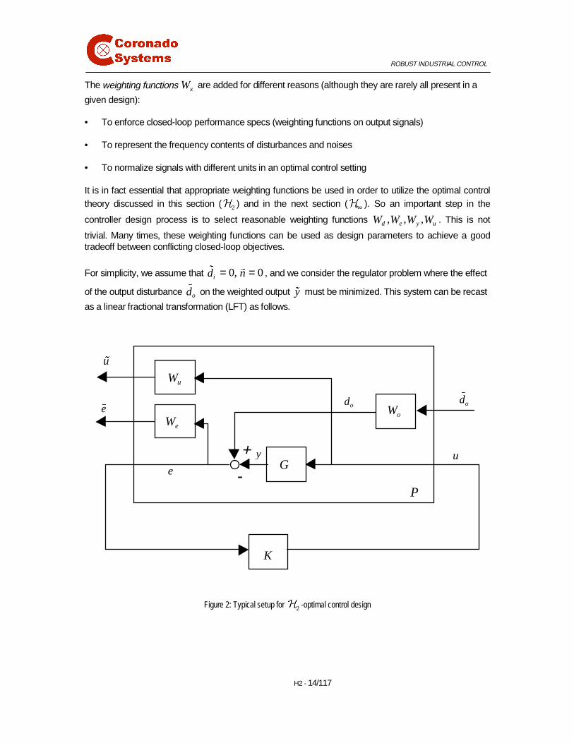
Consider the general block diagram of a feedback control system shown below.
Figure 1: Typical feedback control system
+
-
+ +
+ +
+
+
dy
GKme
uW
odid
y
n
cu u
Py
ny
iWoW
id�cu� od�
yW
eW
nW
y�
ROBUST INDUSTRIAL CONTROL
H2 - 14/117
The weighting functions xW are added for different reasons (although they are rarely all present in a
given design):
• To enforce closed-loop performance specs (weighting functions on output signals)
• To represent the frequency contents of disturbances and noises
• To normalize signals with different units in an optimal control setting
It is in fact essential that appropriate weighting functions be used in order to utilize the optimal controltheory discussed in this section ( 2 ) and in the next section ( ∞ ). So an important step in the
controller design process is to select reasonable weighting functions , , ,d e y uW W W W. This is not
trivial. Many times, these weighting functions can be used as design parameters to achieve a goodtradeoff between conflicting closed-loop objectives.
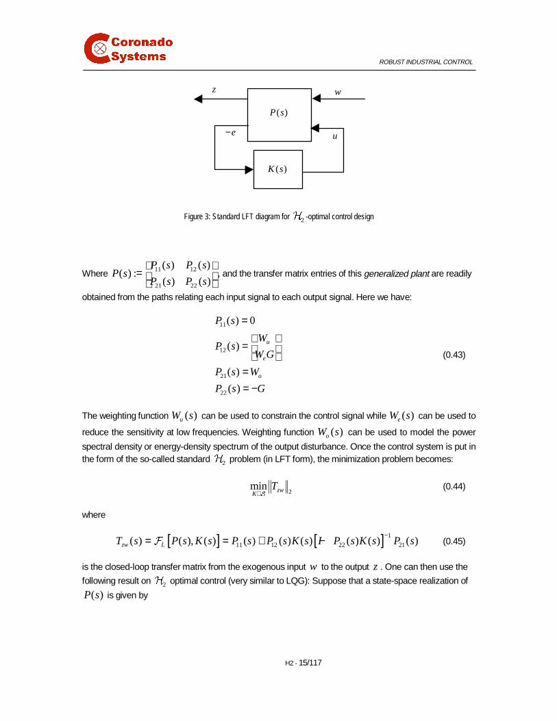
For simplicity, we assume that 0, 0id n= =�
� , and we consider the regulator problem where the effect
of the output disturbance od� on the weighted output y� must be minimized. This system can be recast
as a linear fractional transformation (LFT) as follows.
Figure 2: Typical setup for 2 -optimal control design
+
- G
K
e
uW
od
y u
oW
u�
od�
eWe�
P
ROBUST INDUSTRIAL CONTROL
H2 - 15/117
Figure 3: Standard LFT diagram for 2 -optimal control design
Where 11 12
21 22
( ) ( )( ) :
( ) ( )
P s P sP s
P s P s
=
, and the transfer matrix entries of this generalized plant are readily
obtained from the paths relating each input signal to each output signal. Here we have:
11
12
21
22
( ) 0
( )
( )
( )
u
e
o
P s
WP s
W G
P s W
P s G
=
=
== −
(0.43)
The weighting function ( )uW s can be used to constrain the control signal while ( )eW s can be used to
reduce the sensitivity at low frequencies. Weighting function ( )oW s can be used to model the power
spectral density or energy-density spectrum of the output disturbance. Once the control system is put inthe form of the so-called standard 2 problem (in LFT form), the minimization problem becomes:
2
min zwK
T∈+
(0.44)
where
[ ] [ ] 1
11 12 22 21( ) ( ), ( ) ( ) ( ) ( ) ( ) ( ) ( )zw LT s P s K s P s P s K s I P s K s P s−= = + −� (0.45)
is the closed-loop transfer matrix from the exogenous input w to the output z . One can then use the
following result on 2 optimal control (very similar to LQG): Suppose that a state-space realization of
( )P s is given by
P s( )
wz
−e u
K s( )
ROBUST INDUSTRIAL CONTROL
H2 - 16/117
1 2
1 12
2 21
( ) 0
0
A B B
P s C D
C D
=
(0.46)
Notice the special off-diagonal structure of D : 22D is assumed to be 0 so that 22( )P s is strictly
proper, and 11D is assumed to be 0 so that 11( )P s is also strictly proper (which is a necessary
condition for 11( )P s to be in 2 .)
First define 1 12 12R D D∗= and 2 21 21R D D∗= , and the two Hamiltonian matrices:
( ) ( )1 1
2 1 12 1 2 1 2
2 1 11 12 1 12 1 2 1 12 1
:A B R D C B R B
HC I D R D C A B R D C
− ∗ − ∗
∗∗ − ∗ − ∗
− − = − − − −
(0.47)
( )( ) ( )
1 11 21 2 2 2 2 2
21 1
1 21 2 21 1 1 21 2 2
:A B D R C C R C
JB I D R D B A B D R C
∗∗ − ∗ −
∗ − ∗ ∗ −
− − = − − − −
(0.48)
Note that 2 2, dom(Ric)H J ∈ and 2 2 2 2: Ric( ) 0, : Ric( ) 0X H Y J= ≥ = ≥ . Let us introduce the
concepts of stabilizability and detectability. These are weaker versions of controllability andobservability: they only require that the unstable modes be controllable and observable.
Definition: The pair ( , )A B is said to be stabilizable if there exists a state feedback gain matrix K such
that A BK+ is stable (all eigenvalues have a negative real part).
Definition: The pair ( , )A C is said to be detectable if there exists an observer gain matrix L such that
A LC+ is stable.
Theorem: 2 -Optimal Controller
If the following assumptions hold:
1. The pair 2( , )A B is stabilizable and the pair 2( , )A C is detectable
2. 1 12 12 0R D D∗= > (meaning that all of its eigenvalues are positive) and 2 21 21 0R D D∗= >
3. 2
1 12
A j I B
C D
ω−
has full column rank for all ω
4. 1
2 21
A j I B
C D
ω−
has full row rank for all ω
ROBUST INDUSTRIAL CONTROL
H2 - 17/117
Then, the unique 2 -optimal controller minimizing 2zwT is given by
2 2
2
ˆ( )
0opt
A LK s
F
−=
, (0.49)
where matrix 2L is given by ( ) 12 2 2 1 21 2:L Y C B D R∗ ∗ −= − + , matrix 2F is given by
( )12 1 2 2 12 1:F R B X D C− ∗ ∗= − + , and 2 2 2 2 2
ˆ :A A B F L C= + + .
Remarks:
• Solutions 2 2 2 2: Ric( ), : Ric( )X H Y J= = of the Riccati equations can be obtained using the
Matlab command "lqr".
• The Matlab command "h2syn" directly computes an 2 -optimal controller given the generalized
plant model ( )P s
• Assumptions 3 and 4 ensure that 2 2, dom(Ric)H J ∈
• The assumptions usually hold when the problem is well posed. For example, there should alwaysbe biproper weighting functions on the control signals, otherwise the optimal controller wouldproduce infinite control signals. This corresponds to matrix 12D having full column rank. Likewise,
there should be an output disturbance or a measurement noise defined that couples right into themeasured signal used by the controller. This corresponds to matrix 21D having full column rank.
Example: 2 design for the mixing tank process
The LTI state-space equations for the mixing tank are
[ ]N
7
0
0 0 1 0( )( ) ( )
0.0298 0.001 30 2.388 10
( ) 0 1 ( ) ( )A B
C
d x tx t u t
dt
y t x t d t
−
∆ = ∆ + ∆ − − ×
∆ = ∆ +
������� ������� (0.50)
Recall that the states and inputs are 31 [ ]x V m∆ = ∆ and 2 [ ]x T K∆ = ∆ , and 3
1 [ ]inu q m s∆ = ∆and 2 [ ]u Q W∆ = ∆ . We have already checked that ( , )A B is controllable and ( , )A C is observable.
The plant transfer matrix is given by

ROBUST INDUSTRIAL CONTROL
H2 - 18/117
[ ]
[ ]
[ ]
1
1
7
7
7
ˆ ( )ˆ( ) ( )
ˆ 0( )
0 1 00 1
0.0298 0.001 30 2.388 10
0.001 0 1 010 1
0.0298 30 2.388 10( 0.001)
30 0.0298 2.388 10
( 0.001) ( 0.001)
in A Bq sG s T s
CQ s
C sI A B
s
s
s
ss s
s
s s s
−
−
−
−
−
∆ = ∆ =
∆
= −
= − + − ×
+ = − ×+
− + ×= + +
6
429.8( 1007 1) 2.388 10
(1000 1) (1000 1)s
s s s
−
− + ×= + +
. (0.51)
Assume that the energy-density spectrum (frequency contents) of the output disturbance is mostlyconcentrated below 0.001 radians/s, and is modeled by the biproper weighting function
0.01 10( )
2000 1o
sW s
s
+=+
. (0.52)
The biproper weighting function 10 0
( )0 0.0001uW s
=
is used to constrain the valve and heater
responses, while 10
( )2000 1eW s
s=
+ is used to further reduce the sensitivity at low frequencies.
The generalized plant transfer matrix 11 12
21 22
( ) ( )( ) :
( ) ( )
P s P sP s
P s P s
=
, is obtained from (0.43):

ROBUST INDUSTRIAL CONTROL
H2 - 19/117
11
12 4
3
( ) 0
10 0
0 0.0001( )
10 29.8( 1007 1) 2.388 10
(2000 1) (1000 1) (1000 1)
10 0
0 0.0001
298( 1007 1) 2.388 10
(2000 1)(1000 1) (2000 1)(1000 1)
u
e
P s
WP s
W G s
s s s s
s
s s s s s
−
−
=
= = − + × + + +
=
− + × + + + +
21
4
22
10( )
2000 1
29.8( 1007 1) 2.388 10( )
(1000 1) (1000 1)
oP s Ws
sP s G
s s s
−
= =+
− − + − ×= − = + +
(0.53)
Using the Matlab m-file H2mixing.m, we obtain the fourth-order, proper 2 -optimal controller that
yields 2
1.097zwT = .
��� ,0&+��RSWLPDO /7,FRQWUROOHU
The internal model control (IMC) approach of Morari is well-suited for 2 -optimization. Recall that an
IMC structure uses a nominal internal model of the process and the IMC filter (controller) acts onmeasured output errors between the process and its model. A block diagram of an IMC structure isshown below.
This is the so-called internal model control (IMC) configuration of Morari and Zafiriou (1989) shownbelow. The key assumption here is that the plant, the actuators and the sensors are stable, so that allthe poles of ( ), ( ), ( )a mG s G s G s are in the open left half-plane. Note that the controller is the
feedback interconnection of the extended plant model and the stable IMC controller ( )Q s . Recall that
internal stability of the feedback system is obtained if and only if ( )Q s is stable.
ROBUST INDUSTRIAL CONTROL
H2 - 20/117
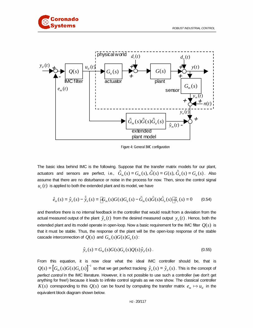
Figure 4: General IMC configuration
The basic idea behind IMC is the following. Suppose that the transfer matrix models for our plant,
actuators and sensors are perfect, i.e., ( ) ( ), ( ) ( ), ( ) ( )m m a aG s G s G s G s G s G s= = =� � � . Also
assume that there are no disturbance or noise in the process for now. Then, since the control signal( )cu t is applied to both the extended plant and its model, we have
ˆˆ ˆ ˆ( ) ( ) ( ) ( ) ( ) ( ) ( ) ( ) ( ) ( ) 0m n n m a m a ce s y s y s G s G s G s G s G s G s u s = − = − = � � �
� (0.54)
and therefore there is no internal feedback in the controller that would result from a deviation from theactual measured output of the plant ( )ny t� from the desired measured output ( )ny t . Hence, both the
extended plant and its model operate in open-loop. Now a basic requirement for the IMC filter ( )Q s is
that it must be stable. Thus, the response of the plant will be the open-loop response of the stablecascade interconnection of ( )Q s and ( ) ( ) ( )m aG s G s G s:
ˆ ˆ( ) ( ) ( ) ( ) ( ) ( )n m a dy s G s G s G s Q s y s= . (0.55)
From this equation, it is now clear what the ideal IMC controller should be, that is
[ ] 1( ) ( ) ( ) ( )m aQ s G s G s G s
−= so that we get perfect tracking ˆ ˆ( ) ( )n dy s y s= . This is the concept of
perfect control in the IMC literature. However, it is not possible to use such a controller (we don't getanything for free!) because it leads to infinite control signals as we now show. The classical controller
( )K s corresponding to this ( )Q s can be found by computing the transfer matrix m de u6 in the
equivalent block diagram shown below.
+
-
+ +
+ +
physical world
sensor
IMC filter actuator plant
+
+
+
- extended plant model
( )dy t
( )my t
( )G s( )Q s
( )me t
( )aG s
( )od t( )id t
y t( )( )du t
( )n t
( )ny t
( ) ( ) ( )m aG s G s G s� � �
( )mG s
( )my t�
ROBUST INDUSTRIAL CONTROL
H2 - 21/117
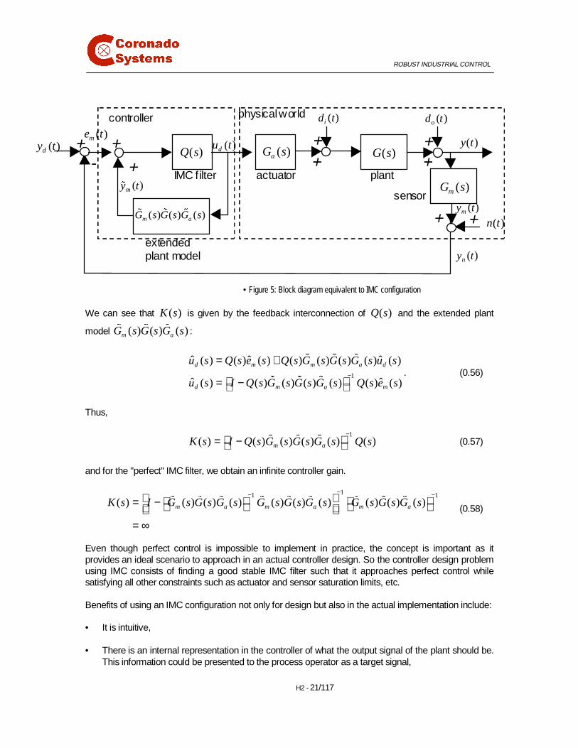
• Figure 5: Block diagram equivalent to IMC configuration
We can see that ( )K s is given by the feedback interconnection of ( )Q s and the extended plant
model ( ) ( ) ( )m aG s G s G s� � � :
1
ˆ ˆ ˆ( ) ( ) ( ) ( ) ( ) ( ) ( ) ( )
ˆ ˆ( ) ( ) ( ) ( ) ( ) ( ) ( )
d m m a d
d m a m
u s Q s e s Q s G s G s G s u s
u s I Q s G s G s G s Q s e s−
= +
= −
� � �
� � �
. (0.56)
Thus,
1( ) ( ) ( ) ( ) ( ) ( )m aK s I Q s G s G s G s Q s
− = −
� � � (0.57)
and for the "perfect" IMC filter, we obtain an infinite controller gain.
11 1( ) ( ) ( ) ( ) ( ) ( ) ( ) ( ) ( ) ( )m a m a m aK s I G s G s G s G s G s G s G s G s G s
−− − = − = ∞
� � � � � � � � �
(0.58)
Even though perfect control is impossible to implement in practice, the concept is important as itprovides an ideal scenario to approach in an actual controller design. So the controller design problemusing IMC consists of finding a good stable IMC filter such that it approaches perfect control whilesatisfying all other constraints such as actuator and sensor saturation limits, etc.
Benefits of using an IMC configuration not only for design but also in the actual implementation include:
• It is intuitive,
• There is an internal representation in the controller of what the output signal of the plant should be.This information could be presented to the process operator as a target signal,
+
-
+ +
+ +
physical world
sensor
IMC filter actuator plant
+
+
+
+
extended plant model
controller
( )dy t
( )my t
( )Q s
( )me t
( )aG s
( )od t( )id t
y t( )( )du t
( )n t
( )ny t
( ) ( ) ( )m aG s G s G s� � �
( )mG s( )my t�
( )G s
ROBUST INDUSTRIAL CONTROL
H2 - 22/117
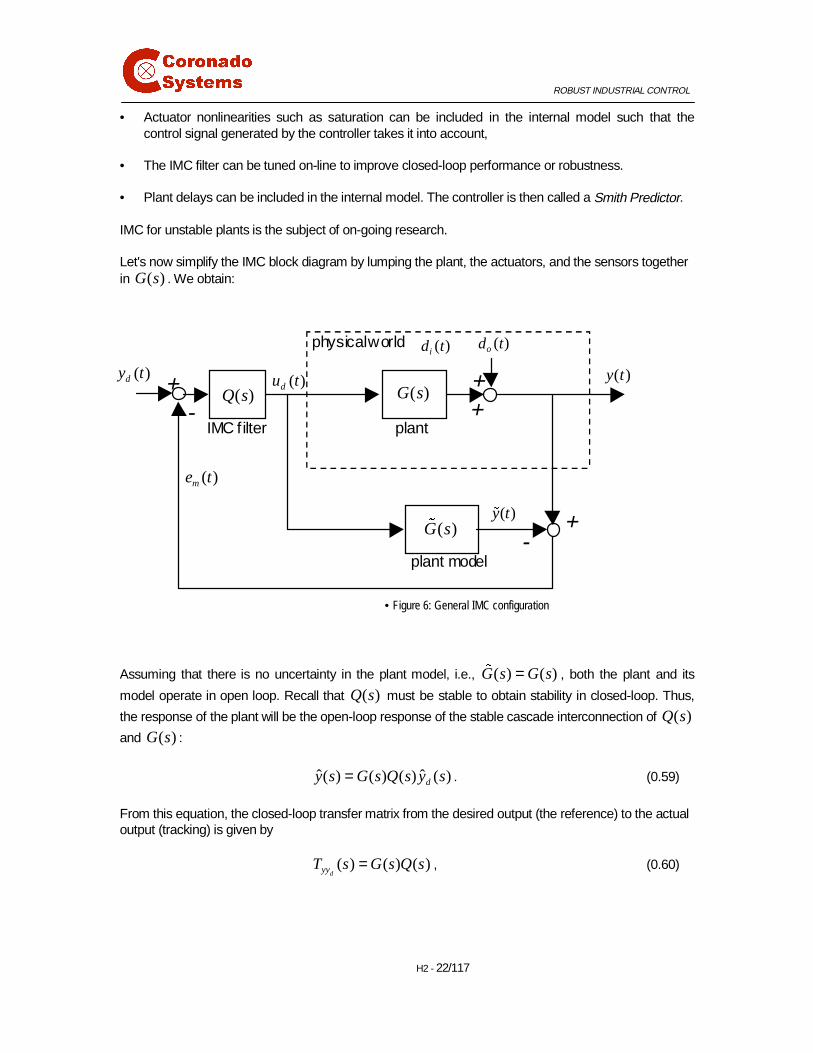
• Actuator nonlinearities such as saturation can be included in the internal model such that thecontrol signal generated by the controller takes it into account,
• The IMC filter can be tuned on-line to improve closed-loop performance or robustness.
• Plant delays can be included in the internal model. The controller is then called a Smith Predictor.
IMC for unstable plants is the subject of on-going research.
Let's now simplify the IMC block diagram by lumping the plant, the actuators, and the sensors togetherin ( )G s . We obtain:
• Figure 6: General IMC configuration
Assuming that there is no uncertainty in the plant model, i.e., ( ) ( )G s G s=� , both the plant and its
model operate in open loop. Recall that ( )Q s must be stable to obtain stability in closed-loop. Thus,
the response of the plant will be the open-loop response of the stable cascade interconnection of ( )Q sand ( )G s :
ˆ ˆ( ) ( ) ( ) ( )dy s G s Q s y s= . (0.59)
From this equation, the closed-loop transfer matrix from the desired output (the reference) to the actualoutput (tracking) is given by
( ) ( ) ( )dyyT s G s Q s= , (0.60)
+
-
+ +
physical world
IMC filter plant
+ -
plant model
( )dy t( )G s( )Q s
( )me t
( )od t( )id t
y t( )( )du t
( )G s�
( )y t�

ROBUST INDUSTRIAL CONTROL
H2 - 23/117
We want to minimize the 2 -norm of the output sensitivity, i.e., the transfer matrix from the output
disturbance to the process output: ˆ ˆ( )oyd oT s d y= 6 . Let's assume for now that ( ) ( )G s G s≠� . The
loop equations are solved by solving for du first:
( ) ( )1 1
ˆ ˆ ˆ ˆ
ˆ ˆ ˆ
d d d
d d
u QGu Qy Qy
u I QG Qy I QG Qy− −
= − +
= − − −
�
� �. (0.61)
The output signal is given by:
ˆˆ ˆd oy Gu d= + . (0.62)
Substituting this expression in (0.61), we obtain:
( ) ( )( ) ( )
( ) ( ) ( )
1 1
1 1
1 11 1 1
ˆˆ ˆ ˆ
ˆˆ ˆ
ˆˆ ˆ
d o
d o
d o
y G I QG Qy G I QG Qy d
I G I QG Q y G I QG Qy d
y I G I QG Q G I QG Qy I G I QG Q d
− −
− −
− −− − −
= − − − +
+ − = − + ⇒
= + − − + + −
� �
� �
� � �
. (0.63)
Therefore,
( )11
oydT I G I QG Q−− = + −
� . (0.64)
Finally, assuming perfect modeling ( ) ( )G s G s=� , we get
( )
( ) ( ) ( )
( )
1 1
11
11
11
(by the "passing through principle": )
( )
oyd
I GQ G G I QG
T I G I QG Q
I I GQ GQ
I GQ I GQ GQ
I GQ
− −
−−
−−
−−
− = −
= + −
= + −
= − − + = −
(0.65)
Note that o dyd yyT T I+ = , which is just the sum of the sensitivity function and the complementary
sensitivity function that we denoted as S T I+ = in the introductory course.
We wish to find ( )Q s ∞∈* such that the 2 -norm 2oydT is minimized, and the minimization
problem can be formulated as:

ROBUST INDUSTRIAL CONTROL
H2 - 24/117
( )2
minQ
I GQ W∞∈
−*
. (0.66)
where ( )W s is a biproper, minimum-phase, stable weighting function that emphasizes frequency
bands (usually low frequencies) where the output sensitivity should be small.
����� 0LQLPXP�SKDVH SODQWV
Suppose that the stable ( )G s is real-rational and minimum-phase, i.e., all of its zeros lie in the open
left half-plane. Then, it is awfully tempting to set 1Q G−= since this IMC filter would be stable and
would reduce the 2 -norm to zero, irrespective of the weighting function. This is the concept of perfect
control again. However, it is not possible to use such a controller because, as shown earlier, it leads toinfinite control signals. Moreover, if ( )G s rolls off at high frequencies, like most processes do, then
1( ) ( )Q j G jω ω−= would tend to infinity as the frequency tends to infinity, which is undesirable
because the closed-loop transfer matrix from the output disturbance to the control signal is given by:
( )( ) ( )1 1
ˆˆ ˆ ˆ ˆ
ˆˆ ˆ
d d d o d
d d o
u QGu Q Gu d Qy
u I QG QG Qy I QG QG Qd− −
= − + +
= − + − − +
�
� �
(0.67)
which for ( ) ( )G s G s=� simplifies to:
d ou dT Q= − . (0.68)
The optimization of (0.66) is not well-posed. One would have to add the norm of the closed-loop matrixfrom the output disturbance to the control signal in (0.66) to make it well-posed. Nevertheless, Morariand Zafiriou proposed the concept of an IMC filter that is split up between a part that inverts theprocess, and another part that rolls off at high frequencies (the tuning filter) to make sure that theactuators won't respond violently to high-frequency disturbances or measurement noise. Assuming that
( )G s is real-rational and minimum-phase, the IMC controller is proposed as
1fQ G Q−= . (0.69)
This controller isn't optimal in the sense that it doesn't minimize (0.66) (in fact, it can make the norminfinite!), but fQ can be chosen such that it is close to the identity at low frequencies where a low
sensitivity is important, and that rolls off faster than the process so that 1fQ G Q−= is strictly proper
and thus rolls off at high frequencies.
Example (IMC design simple first-order SISO minimum-phase plant)
Consider the process described by its transfer function 2
( )1
G ss
=+
and assume that the model is
perfect. An IMC controller for this process could be chosen as
ROBUST INDUSTRIAL CONTROL
H2 - 25/117
12
1 1 1 1
2 2 ( 1) 2( 1)f f
s sQ G Q Q
s s− + += = = =
+ +. (0.70)
Which would yield the output sensitivity
2 2
1 ( 2)1 1
( 1) ( 1)oyd
s sT GQ
s s
+= − = − =+ +
(0.71)
and the complementary sensitivity
2
1
( 1)dyy fT GQ Qs
= = =+
. (0.72)
We see that the tuning filter fQ directly specifies the complementary sensitivity function from the
reference to the output: dyy fT Q= . Hence tracking performance is specified by fQ .
����� 1RQ�PLQLPXP�SKDVH SODQWV
For non-minimum-phase plants (including plants with delays), we can't invert ( )G s with ( )Q s as this
would result in an unstable ( )Q s , and hence an unstable control system. What we can do is to invert
the invertible (minimum-phase) part of ( )G s . The minimization problem was formulated as:
( )2
2
min
min
Q
Q
I GQ W
W GQ
∞
∞
∈
∈
−
≡ −
*
*
. (0.73)
Write ( )G s as a product of two transfer matrices, one that's all-pass and one that's minimum-phase:
( ) ( ) ( )ap mpG s G s G s= . (0.74)
The all-pass factor ( )apG s has all the RHP zeros of ( )G s and satisfies ( ) ( )ap apG j G j Iω ω∗ = . Let
~ ( ) : ( )Tap apG s G s= − . It is easy to show that if 2( )apG s ∈ , then ~
2( )apG s ⊥∈ . The latter is also all-
pass. Then ( )apG s is such that ~ ( ) ( )ap apG s G s I= , hence ~ 1( ) ( )ap apG s G s−= . We have
2 2ap mpW GQ W G G Q− = − . (0.75)
It can be shown that the 2 -norm of a transfer matrix is invariant under multiplication by an all-pass
function, thus

ROBUST INDUSTRIAL CONTROL
H2 - 26/117
N N
{ } { }
{ } { }
2
22
2 2
~ 22
~ ~ 22
2 2~ ~
2 2
|| ||
|| ||
ap mp
ap mp
ap ap mp
ap ap mp
W GQ W G G Q
G W G Q
G W G W G Q
G W G W G Q
⊥
⊥
⊥
⊥
∈ ⊕ ∈
∈ ∈
− = −
= −
= + −
= + −
� �
� �
� �
� �
��� �������
. (0.76)
where { }~apG W
�
means taking the stable terms (with LHP poles) in the partial fraction expansion of
~apG W , and { }~
apG W ⊥�
means taking the unstable terms (with RHP poles) in the partial fraction
expansion of ~apG W
Clearly from (0.76), the optimal normalized IMC controller is given by { }1 ~mp apQ G G W−=
�
, and the
actual IMC controller is { }1 ~ 1mp apQ G G W W− −=
�
. Then the sensitivity and complementary sensitivity
functions are:
{ } { }{ } { }
1 ~ 1 ~ 1
1 ~ 1 ~ 1
o
d
yd mp ap ap ap
yy mp ap ap ap
T I GQ I GG G W W I G G W W
T GQ GG G W W G G W W
− − −
− − −
= − = − = −
= = =
H H
H H
� �
� �
. (0.77)
Example: SISO 2 -optimal IMC design
Consider the nonminimum-phase process model
29.8( 1007 1)( )
(500 1)(1000 1)s
G ss s
− +=+ +
. (0.78)
We wish to design an 2 -optimal IMC controller for this process. The transfer function is factorized as
a product of an allpass transfer function and a minimum-phase transfer function:
( ) ( )
( 1007 1) 29.8(1007 1)( )
(1007 1) (500 1)(1000 1)
ap mpG s G s
s sG s
s s s
− + +=+ + +
������������
(0.79)
with the weighting function representing the spectral contents of the output disturbance
100( )
2000 1W s
s=
+. (0.80)

ROBUST INDUSTRIAL CONTROL
H2 - 27/117
The optimal IMC controller is given by { }1 ~ 1mp apQ G G W W− −=
�
. We need to compute { }~apG W
H�
first
using a partial fraction expansion:
~ 100(1007 1)( ) ( )
( 1007 1)(2000 1)
0.0665 0.0165
1 1007 1 2000
ap
sG s W s
s s
s s
+=− + +−= +− +
(0.81)
Thus, { }~ 0.0165
1 2000apG Ws
=+�
, the stable part. Finally, the optimal IMC controller is computed to be
{ }1 ~ 1
(500 1)(1000 1) 0.0165 2000 1
29.8(1007 1) 1 2000 100
(500 1)(1000 1)0.0111
(1007 1)
mp apQ G G W W
s s s
s s
s s
s
− −=
+ + + = + + + +=
+
H�
(0.82)
Notice that this optimal IMC controller isn’t proper, so it is appropriate to add a high-frequency pole1
( ) :0.001 1fQ s
s=
+ which will not disturb ( )Q s at frequencies of interest:
(500 1)(1000 1)
0.0111(1007 1)(0.001 1)
s sQ
s s
+ +=+ +
(0.83)
The sensitivity and complementary sensitivity functions are then given by:
{ }{ }
1 ~ 1
~ 1
2
1 1
1
( 1007 1) 0.0165 2000 11
(1007 1) 1 2000 100(0.001 1)
( 1007 1) 1.007 1339.3 0.671 0.33
(1007 1)(0.001 1) (1007 1)(0.001 1)
1
o
d
yd mp ap f
ap ap f
yy
T GQ GG G W W Q
G G W W Q
s s
s s s
s s s
s s s s
T GQ
− −
−
= − = −
= −
− + += − + + + − + + += − =
+ + + +
= =
�
�
( 1007 1)0.33
(1007 1)(0.001 1)oyd
sT
s s
− +− =+ +
. (0.84)
A Bode plot of the sensitivity if shown below.
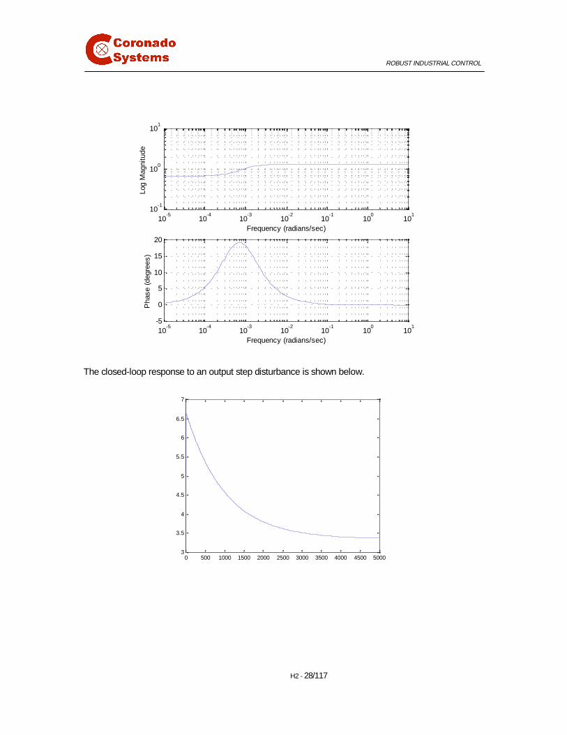
ROBUST INDUSTRIAL CONTROL
H2 - 28/117
The closed-loop response to an output step disturbance is shown below.
10-5
10-4
10-3
10-2
10-1
100
101
10-1
100
101
Log
Mag
nitu
de
Frequency (radians/sec)
10-5
10-4
10-3
10-2
10-1
100
101
-5
0
5
10
15
20
Pha
se (
degr
ees)
Frequency (radians/sec)
0 500 1000 1500 2000 2500 3000 3500 4000 4500 50003
3.5
4
4.5
5
5.5
6
6.5
7
ROBUST INDUSTRIAL CONTROL
H2 - 29/117
� +∞ 2SWLPDO &RQWURO
∞ optimal control is a theory to design finite-dimensional stabilizing LTI controllers that minimize the
∞ -norm of the closed-loop system.
��� 3UREOHPVHWXS
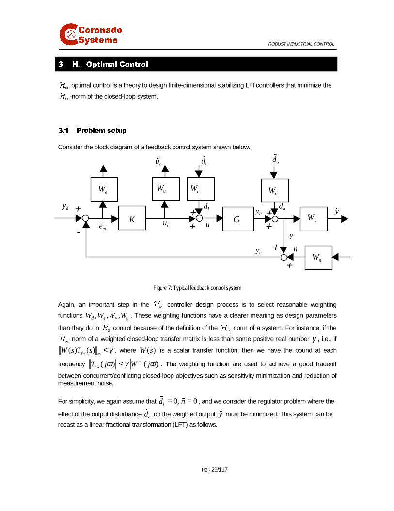
Consider the block diagram of a feedback control system shown below.
Figure 7: Typical feedback control system
Again, an important step in the ∞ controller design process is to select reasonable weighting
functions , , ,d e y uW W W W. These weighting functions have a clearer meaning as design parameters
than they do in 2 control because of the definition of the ∞ norm of a system. For instance, if the
∞ norm of a weighted closed-loop transfer matrix is less than some positive real number γ , i.e., if
( ) ( )zwW s T s γ∞
< , where ( )W s is a scalar transfer function, then we have the bound at each
frequency 1( ) ( )zwT j W jω γ ω−< . The weighting function are used to achieve a good tradeoff
between concurrent/conflicting closed-loop objectives such as sensitivity minimization and reduction ofmeasurement noise.
For simplicity, we again assume that 0, 0id n= =�
� , and we consider the regulator problem where the
effect of the output disturbance od� on the weighted output y� must be minimized. This system can be
recast as a linear fractional transformation (LFT) as follows.
+
-
+ +
+ +
+
+
dy
GKme
uW
odid
y
n
cu u
Py
ny
iWoW
id�cu� od�
yW
eW
nW
y�
ROBUST INDUSTRIAL CONTROL
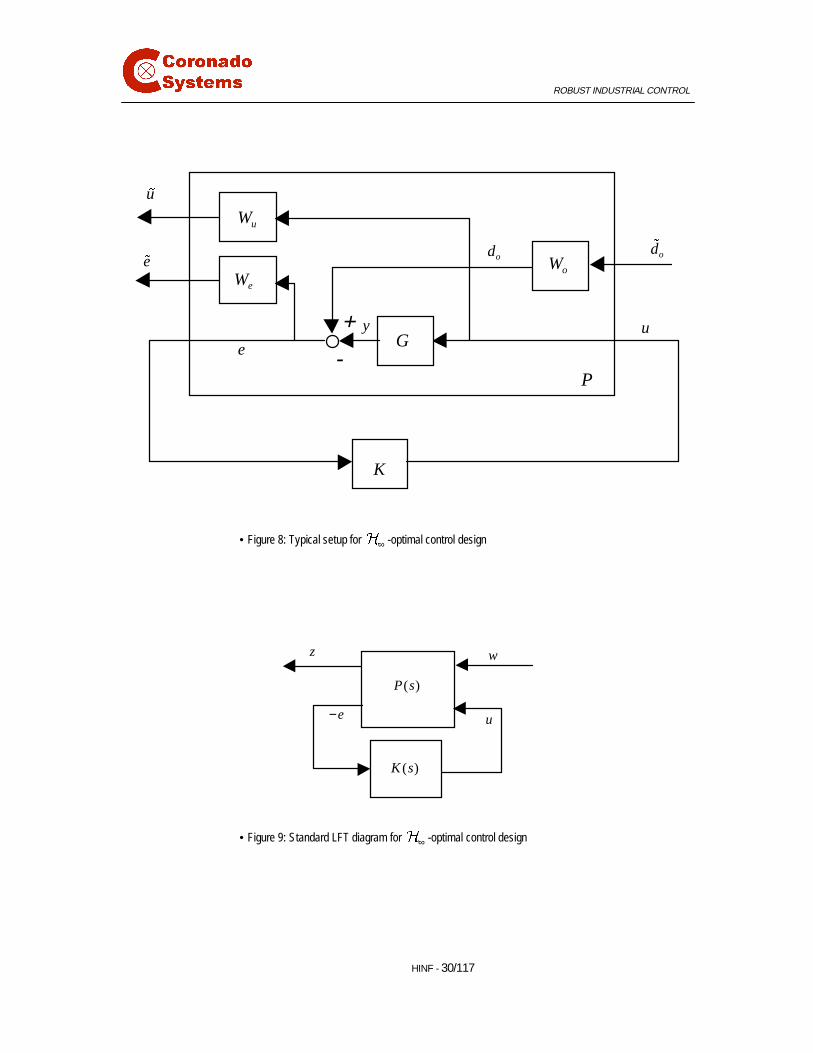
HINF - 30/117
• Figure 8: Typical setup for ∞ -optimal control design
• Figure 9: Standard LFT diagram for ∞ -optimal control design
+
- G
K
e
uW
od
y u
oW
u�
od�
eWe�
P
P s( )
wz
−e u
K s( )
ROBUST INDUSTRIAL CONTROL
HINF - 31/117
Where 11 12
21 22
( ) ( )( ) :
( ) ( )
P s P sP s
P s P s
=
, and the transfer matrix entries of this generalized plant were given
in (0.43) and are repeated here for convenience:
11
12
21
22
( ) 0
( )
( )
( )
u
e
o
P s
WP s
W G
P s W
P s G
=
=
== −
(0.85)
The weighting function ( )uW s can be used to constrain the control signal at each frequency, while
( )eW s can be used to reduce the sensitivity, typically at low frequencies. Weighting function ( )oW scan be used to model the power spectral density or energy-density spectrum of the output disturbance.Once the control system is put in the form of the so-called standard ∞ problem (in LFT form), the
minimization problem becomes:
min zwK
T∞∈+
(0.86)
where [ ]( ) ( ), ( )zw LT s P s K s= � is the closed-loop transfer matrix from the exogenous input w to
the output z . The optimization of (0.86) is very difficult theoretically and numerically. Virtuallyeverybody uses the solution to the suboptimal ∞ problem stated as
Given 0γ > , find an admissible controller (if there exists any) such that zwT γ∞
< .
We will present the solution to this problem, and it should be clear that an iterative bisection procedurefor reducing γ while checking that a suboptimal controller exists will lead to a controller as close to the
optimal controller as desired.
��� 6ROXWLRQ WR VLPSOLILHG VXERSWLPDO ∞ SUREOHP
The solution to the simplified suboptimal ∞ problem is obtained from the solutions of a pair of Riccati
equations. However, the difference with the 2 problem is that these Riccati equations cannot be
solved independently from one another, making the ∞ problem more difficult.
But first, let's discuss the simplifying assumptions that we will use here. The general problem is moreinvolved mathematically, and doesn't provide much more insight. Therefore we will stick with thesimplified problem.
Suppose that a state-space realization of the generalized plant ( )P s is given by

ROBUST INDUSTRIAL CONTROL
HINF - 32/117
1 2
1 12
2 21
( ) 0
0
A B B
P s C D
C D
=
. (0.87)
Notice the special off-diagonal structure assumed for D (just like the 2 case). Given 0γ > , define
the two Hamiltonian matrices:
21 1 2 2
1 1
:A B B B B
HC C A
γ − ∗ ∗
∞ ∗ ∗
−=
− − , (0.88)
21 1 2 2
1 1
:A C C C C
JB B A
γ∗ − ∗ ∗
∞ ∗
−=
− − . (0.89)
Assume that:
1. The pair 1( , )A B is stabilizable and the pair 1( , )A C is detectable,
2. The pair 2( , )A B is stabilizable and the pair 2( , )A C is detectable,
3. [ ]12 1 12 0TD C D I = (meaning that the columns of 12D are orthonormal, and orthogonal to
the columns of 1C )
4. 121
21
0TBD
D I
=
(meaning that the rows of 21D are orthonormal, and orthogonal to the rows of
1B )
Remarks:
• Assumption 2 is required if we want to stabilize the plant with the controller
• Assumption 1 simplifies the theoretical developments and usually holds in practice
• Assumptions 3 and 4 are also made for technical reasons and practical problems can be set up sothat these assumptions hold.
Theorem: ∞ Controller
There exists an admissible controller such that zwT γ∞
< if and only if the following three conditions
hold:
ROBUST INDUSTRIAL CONTROL
HINF - 33/117
1. dom(Ric)H∞ ∈ and : Ric( ) 0X H∞ ∞= ≥ ;
2. dom(Ric)J∞ ∈ and : Ric( ) 0Y J∞ ∞= ≥ ;
3. ( ) 2X Yρ γ∞ ∞ < (the spectral radius of the product X Y∞ ∞ )
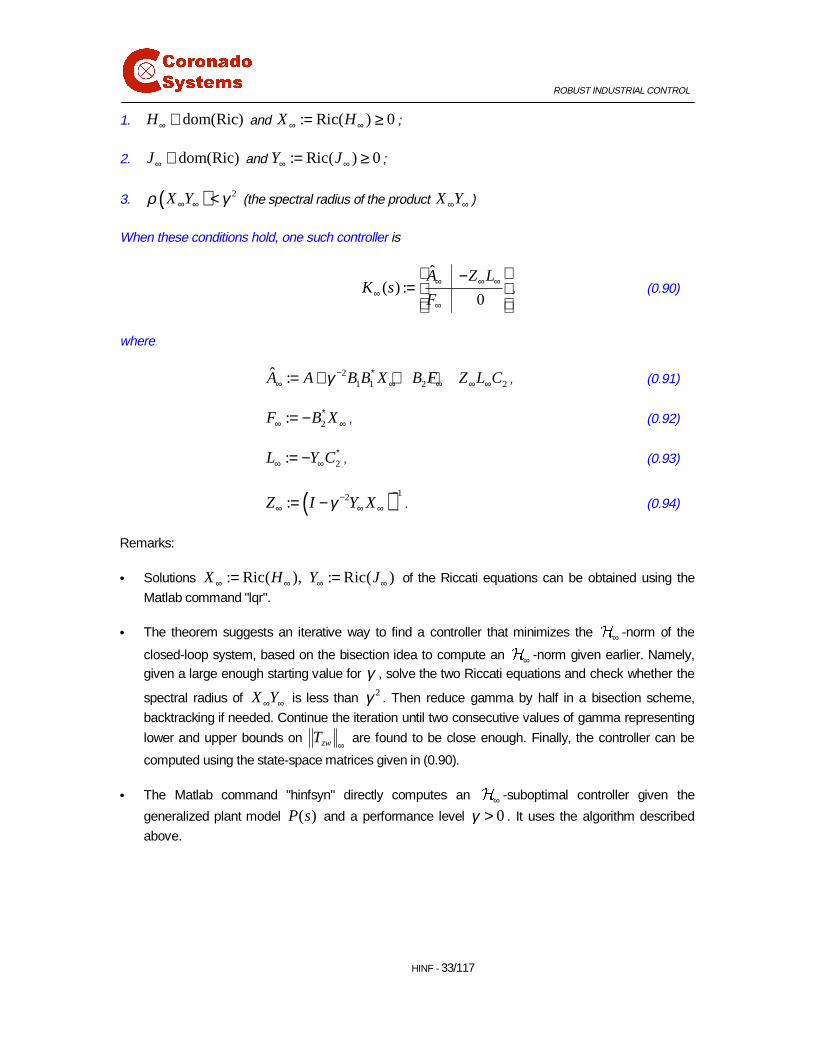
When these conditions hold, one such controller is
ˆ( ) :
0
A Z LK s
F∞ ∞ ∞
∞∞
−=
, (0.90)
where
21 1 2 2
ˆ :A A B B X B F Z L Cγ − ∗∞ ∞ ∞ ∞ ∞= + + + , (0.91)
2:F B X∗∞ ∞= − , (0.92)
2:L Y C∗∞ ∞= − , (0.93)
( ) 12:Z I Y Xγ−−
∞ ∞ ∞= − . (0.94)
Remarks:
• Solutions : Ric( ), : Ric( )X H Y J∞ ∞ ∞ ∞= = of the Riccati equations can be obtained using the
Matlab command "lqr".
• The theorem suggests an iterative way to find a controller that minimizes the ∞ -norm of the
closed-loop system, based on the bisection idea to compute an ∞ -norm given earlier. Namely,given a large enough starting value for γ , solve the two Riccati equations and check whether the
spectral radius of X Y∞ ∞ is less than 2γ . Then reduce gamma by half in a bisection scheme,
backtracking if needed. Continue the iteration until two consecutive values of gamma representing
lower and upper bounds on zwT∞
are found to be close enough. Finally, the controller can be
computed using the state-space matrices given in (0.90).
• The Matlab command "hinfsyn" directly computes an ∞ -suboptimal controller given the
generalized plant model ( )P s and a performance level 0γ > . It uses the algorithm described
above.

ROBUST INDUSTRIAL CONTROL
HINF - 34/117
Example: ∞ design for the mixing tank process
The plant transfer matrix is given by
4ˆ ( ) 29.8( 1007 1) 2.388 10ˆ( ) ( )ˆ (1000 1) (1000 1)( )
inq s sG s T s
s s sQ s
−∆ − + ×= ∆ = + +∆ 6 . (0.95)
Assume that the energy-density spectrum (frequency contents) of the output disturbance is mostlyconcentrated below 0.001 radians/s, and is modeled by the biproper weighting function
0.01 10( )
2000 1o
sW s
s
+=+
. (0.96)
The biproper weighting function 10 0
( )0 0.0001uW s
=
is used to constrain the valve and heater
responses, while 10
( )2000 1eW s
s=
+ is used to further reduce the sensitivity at low frequencies. We
also use an input weighting ( ) 0.001iW s = to satisfy Assumption 1 ( 1( , )A B must be stabilizable.)
The generalized plant transfer matrix 11 12
21 22
( ) ( )( ) :
( ) ( )
P s P sP s
P s P s
=
, was obtained in (0.43).
Using the Matlab m-file Hinfmixing.m, we obtain the following output from hinfsyn (bisection):
Test bounds: 0.0000 < gamma <= 1000.0000
gamma hamx_eig xinf_eig hamy_eig yinf_eig nrho_xy p/f
1.000e+003 5.0e-004 2.2e-013 4.0e-004 -4.3e-018 0.0006 p
500.000 5.0e-004 2.2e-013 4.0e-004 -4.5e-017 0.0023 p
250.000 5.0e-004 2.2e-013 4.0e-004 -6.8e-018 0.0094 p
125.000 5.0e-004 2.2e-013 4.0e-004 -1.5e-017 0.0376 p
62.500 5.0e-004 2.2e-013 4.0e-004 -3.3e-018 0.1505 p
31.250 5.0e-004 2.2e-013 4.0e-004 -1.9e-017 0.6054 p
15.625 5.0e-004 2.2e-013 4.0e-004 -2.3e-018 2.4768# f
27.057 5.0e-004 2.2e-013 4.0e-004 -8.0e-017 0.8096 p
24.771 5.0e-004 2.2e-013 4.0e-004 -1.3e-017 0.9678 p
22.941 5.0e-004 2.2e-013 4.0e-004 -3.8e-017 1.1305# f
24.270 5.0e-004 2.2e-013 4.0e-004 7.1e-018 1.0086# f
Gamma value achieved: 24.7705
norm between 24.7674 and 24.7921
achieved near 0

ROBUST INDUSTRIAL CONTROL
HINF - 35/117
This indicates that the achieved ∞ -norm is 24.77zwT ∞ = . The fourth-order ∞ controller in the
form ( )A B
K sC D
=
displayed below:
-8.3e+001 3.2e-017 0.0e+000 -1.2e+003 | -3.1e+005
-8.7e-019 -4.0e-004 0.0e+000 0.0e+000 | -1.7e+001
-1.4e+001 -1.5e-002 -2.1e+001 -2.0e+002 | -5.3e+004
-4.2e+002 4.5e-001 6.2e+002 -6.0e+003 | -1.6e+006
------------------------------------------------------------|----------
-2.4e-004 -5.7e-005 -7.8e-002 -2.6e-003 | 0.0e+000
-8.6e+001 -2.8e+001 -2.7e+004 -9.1e+002 | 0.0e+000
ROBUST INDUSTRIAL CONTROL
UNC - 36/117
� 8QFHUWDLQW\ 0RGHOLQJ IRU 5REXVW &RQWURO
Any mathematical representation (model) of a physical process needs approximations, which lead tomodel uncertainties. Different forms of models exist to represent these uncertainties according to whatinformation we want to include in the model. These representations reflect at the same time theknowledge of the physical phenomena that cause these uncertainties and our capacity to representthem in a form that's easy to manipulate.
Consider an aircraft as a physical example, whose parameters vary with the flight conditions (altitude,velocity). Certainly, we can obtain a linear mathematical model for a such system by linearizing theequations of the aircraft at different flight conditions within the flight envelope. This will lead to aninterval of variation for each parameter of the model obtained. These intervals of parameter uncertaintymay represent structurally and accurately the uncertainties in the model but are not easy to deal withmathematically. On the other hand, we can use a more global representation of the uncertainties as adynamical perturbation of a nominal transfer matrix.
��� 8QVWUXFWXUHGXQFHUWDLQW\
����� $GGLWLYH XQFHUWDLQW\ PRGHO
Suppose that the unknown transfer matrix ( )pG s of a process differs from a nominal transfer matrix
model ( )G s that we have of it. We say that ( )pG s is the perturbed model and ( )G s is the nominal
model. The difference between these two models comes from an unknown dynamical perturbation( )s∆ representing the unmodeled dynamics of the process. Suppose that this perturbation is additive,
call it ( )a s∆ , and that we know a function ( ) 0aδ ω ≥ that bounds its norm (maximum singular value)
for each frequency:
( ) ( ) ( )p aG s G s s= + ∆ (0.97)
with ( ) ( ),a ajω δ ω ω∆ < ∀ . (0.98)
Note that the upper bound ( )aδ ω represent the "size" of the uncertainty of the model at each
frequency. It is often taken to be the magnitude of a scalar transfer function. This form of representationis called additive uncertainty because the perturbation's transfer matrix is added to the nominal model.This type of uncertainty is also called unstructured because the only information we use is just theupper bound of the norm of the uncertainty, and not its structure. That is, ( )a s∆ can be any transfer
matrix that satisfies (0.98).
The figure below shows a closed loop system with such an additive uncertainty model. Again, it isimportant to emphasize that we don't know what ( )a s∆ is, we only know that it is bounded by
( ) ( ),a ajω δ ω ω∆ < ∀ .
We can define a family of perturbed plant models as the set
ROBUST INDUSTRIAL CONTROL
UNC - 37/117
{ }: ( ) : ( ) ( )p a aG s jω δ ω= ∆ <( . (0.99)
Then, robust control theory assumes that the unknown, "true" plant model belongs to ( . Thus, robustcontrol design consists of designing a controller that can maintain a desired performance level for allplants in ( (robust performance) or just stabilize all plants in ( (robust stability).
Returning to the aircraft example, we might choose the nominal model ( )G s as the transfer matrix
corresponding to an average flight condition. We can obtain ( )aδ ω by calculating a large, but finite
number of perturbed transfer matrices { }1
( )N
pi iG s
= corresponding to various possible flight conditions
(altitudes and Mach numbers). It is then reasonable to expect that the corresponding additiveperturbation ( )a s∆ would be bounded by:
1, ,max ( ) ( )pi
i NG j G jω ω
=−
!
(0.100)
at each frequency. We would then try to find an uncertainty bound ( )aδ ω such that
1, ,max ( ) ( ) ( )pi a
i NG j G jω ω δ ω
=− <
!
. (0.101)
To avoid getting too much uncertainty in the model, the upper bound ( )aδ ω should be "tight", i.e., it
should be close to the left-hand side of (0.101). This would prevent a subsequent robust controllerdesign to be too conservative, i.e., robust to more uncertainty than warranted by our knowledge of theprocess, but with poor performance. In other words, putting too much uncertainty in the model may bedetrimental to the achievable closed-loop performance level. This is an expression of the well-knownrobustness/performance tradeoff of feedback control.
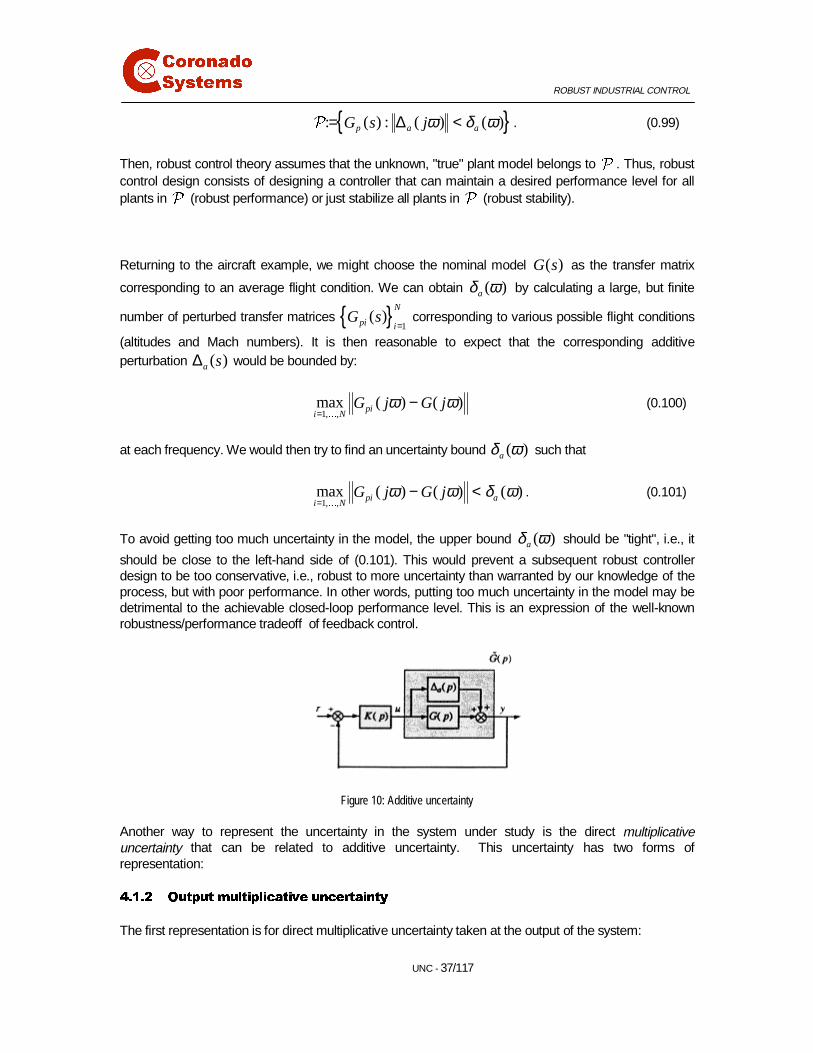
Figure 10: Additive uncertainty
Another way to represent the uncertainty in the system under study is the direct multiplicativeuncertainty that can be related to additive uncertainty. This uncertainty has two forms ofrepresentation:
����� 2XWSXWPXOWLSOLFDWLYH XQFHUWDLQW\
The first representation is for direct multiplicative uncertainty taken at the output of the system:
ROBUST INDUSTRIAL CONTROL
UNC - 38/117
( ) ( ( )) ( )p p mG j I j G jω ω ω= + ∆ (0.102)
with ( ) ( )m mjω δ ω∆ < ω∀ . (0.103)
Figure 11: Output multiplicative uncertainty
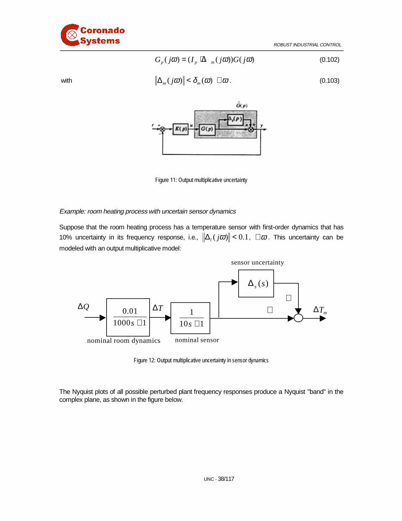
Example: room heating process with uncertain sensor dynamics
Suppose that the room heating process has a temperature sensor with first-order dynamics that has
10% uncertainty in its frequency response, i.e., ( ) 0.1l jω∆ < , ω∀ . This uncertainty can be
modeled with an output multiplicative model:
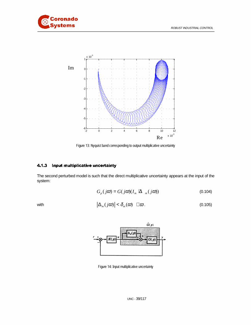
Figure 12: Output multiplicative uncertainty in sensor dynamics
The Nyquist plots of all possible perturbed plant frequency responses produce a Nyquist "band" in thecomplex plane, as shown in the figure below.
0.01
1000 1s +
( )s s∆
1
10 1s +
++
nominal sensornominal room dynamics
sensor uncertainty
Q∆ T∆mT∆
ROBUST INDUSTRIAL CONTROL
UNC - 39/117
Figure 13: Nyquist band corresponding to output multiplicative uncertainty
����� ,QSXWPXOWLSOLFDWLYH XQFHUWDLQW\
The second perturbed model is such that the direct multiplicative uncertainty appears at the input of thesystem:
( ) ( )( ( ))p m mG j G j I jω ω ω= + ∆ (0.104)
with ( ) ( )m mjω δ ω∆ < ω∀ . (0.105)
Figure 14: Input multiplicative uncertainty
-2 0 2 4 6 8 10 12
x 10-3
-6
-5
-4
-3
-2
-1
0
1x 10
-3
Im
Re
ROBUST INDUSTRIAL CONTROL
UNC - 40/117
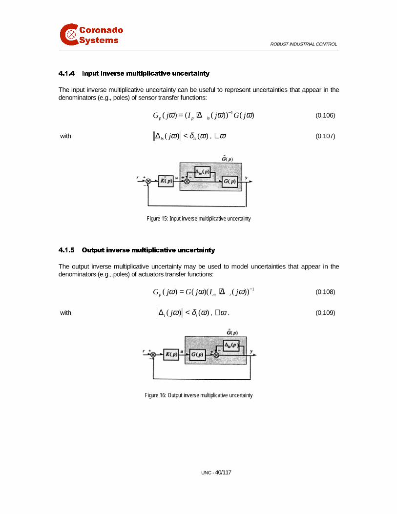
����� ,QSXW LQYHUVHPXOWLSOLFDWLYH XQFHUWDLQW\
The input inverse multiplicative uncertainty can be useful to represent uncertainties that appear in thedenominators (e.g., poles) of sensor transfer functions:
1( ) ( ( )) ( )p p isG j I j G jω ω ω−= + ∆ (0.106)
with ( ) ( )is isjω δ ω∆ < , ω∀ (0.107)
Figure 15: Input inverse multiplicative uncertainty
����� 2XWSXW LQYHUVHPXOWLSOLFDWLYH XQFHUWDLQW\
The output inverse multiplicative uncertainty may be used to model uncertainties that appear in thedenominators (e.g., poles) of actuators transfer functions:
1( ) ( )( ( ))p m iG j G j I jω ω ω −= + ∆ (0.108)
with ( ) ( )i ijω δ ω∆ < , ω∀ . (0.109)
Figure 16: Output inverse multiplicative uncertainty
ROBUST INDUSTRIAL CONTROL
UNC - 41/117
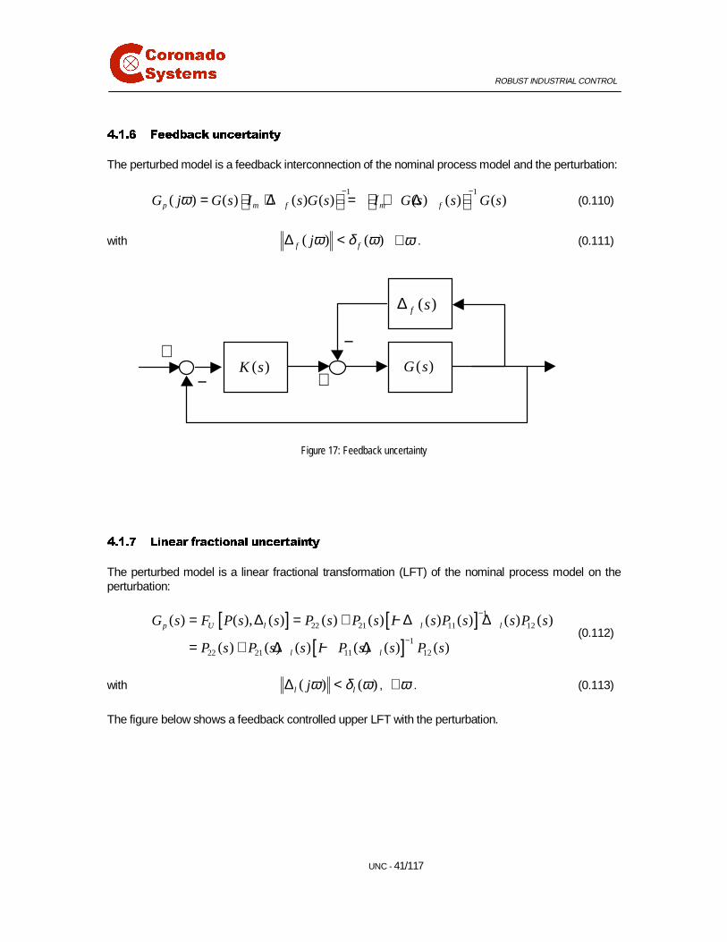
����� )HHGEDFN XQFHUWDLQW\
The perturbed model is a feedback interconnection of the nominal process model and the perturbation:
1 1( ) ( ) ( ) ( ) ( ) ( ) ( )p m f m fG j G s I s G s I G s s G sω
− − = + ∆ = + ∆ (0.110)
with ( ) ( )f fjω δ ω∆ < ω∀ . (0.111)
Figure 17: Feedback uncertainty
����� /LQHDU IUDFWLRQDO XQFHUWDLQW\
The perturbed model is a linear fractional transformation (LFT) of the nominal process model on theperturbation:
[ ] [ ][ ]
1
22 21 11 12
1
22 21 11 12
( ) ( ), ( ) ( ) ( ) ( ) ( ) ( ) ( )
( ) ( ) ( ) ( ) ( ) ( )
p U l l l
l l
G s F P s s P s P s I s P s s P s
P s P s s I P s s P s
−
−
= ∆ = + − ∆ ∆
= + ∆ − ∆(0.112)
with ( ) ( )l ljω δ ω∆ < , ω∀ . (0.113)
The figure below shows a feedback controlled upper LFT with the perturbation.
( )G s
( )f s∆
−
+( )K s
−
+
ROBUST INDUSTRIAL CONTROL
UNC - 42/117
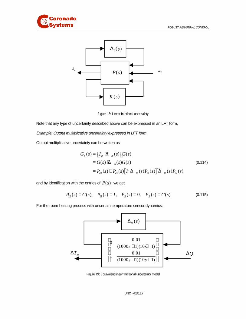
Figure 18: Linear fractional uncertainty
Note that any type of uncertainty described above can be expressed in an LFT form.
Example: Output multiplicative uncertainty expressed in LFT form
Output multiplicative uncertainty can be written as
[ ] 1
22 21 11 12
( ) ( ) ( )
( ) ( ) ( )
( ) ( ) ( ) ( ) ( ) ( )
p p m
m
m m
G s I s G s
G s s G s
P s P s I s P s s P s−
= + ∆ = + ∆
= + − ∆ ∆
(0.114)
and by identification with the entries of ( )P s , we get
22 21 11 12( ) ( ), ( ) , ( ) 0, ( ) ( )P s G s P s I P s P s G s= = = = (0.115)
For the room heating process with uncertain temperature sensor dynamics:
Figure 19: Equivalent linear fractional uncertainty model
P s( )
( )l s∆
2z2w
( )K s
0.010
(1000 1)(10 1)
0.011
(1000 1)(10 1)
s s
s s
+ + + +
( )m s∆
Q∆mT∆
ROBUST INDUSTRIAL CONTROL
UNC - 43/117
Certainly, with such unstructured uncertainty models, we can be conservative and even lose someinformation about the uncertainty in the physical system, but these kinds of models are general and canrepresent, lumped into the same model, different uncertainties of different natures. Consider differenttypes on uncertainties and see what perturbation models can represent these uncertainties:
Unmodeled process dynamics at high frequencies: Uncertainty in the roll-off rate of the process modelcan be represented by multiplicative uncertainty models, or the additive uncertainty model.
Parametric uncertainty: Variation in the model parameters can be represented by the additiveuncertainty model, the direct multiplicative model and also the inverse model if the system is square by
comparing 1( )G jω − and 1( )pG jω − .
Actuator uncertainty: This type of uncertainty essentially comes from the fact that the dynamics of theprocess actuators may not be well known, or may have been neglected. These uncertainties can betake into account by using the two forms of direct and inverse multiplicative uncertainty at the input.
Sensor uncertainty: Sensors are often sensitive devices that can be partially damaged and deliverslightly erroneous measures. Sensor uncertainty can be represented by the direct and the reversemultiplicative uncertainties at the output.
Nonlinearity and reduction of the model:: Non-linearities can be taken into account if their effect can bebounded in the frequency domain (this is not always the case!). Model reduction is often used tosimplify the control design. When model reduction techniques are used, we can take into account theneglected dynamics as uncertainty that can be represented by any type of model uncertainty.
����� 5HSUHVHQWLQJ XQFHUWDLQW\ LQ WKH IUHTXHQF\ GRPDLQ
The frequency domain approach, and more specifically the ∞ theory, gives the necessary tools to
quantify the uncertainties modeled for the physical system under study. Through the example below,we give more details on how the uncertainty regions could be represented by a complex norm-boundedperturbation around a nominal plant.
Suppose we have the perturbed SISO system:
( ) ( ) ( ) ( )p a aG s G s W s s= + ∆� , (0.116)
( ) 1a jω∆ < , ω∀ (0.117)
where ( )a s∆� is any stable transfer function which, at each frequency, is no larger than one in
magnitude (the tilde indicates normalization), and ( )aW s is a weighting function bounding the
uncertainty. This means that at each frequency, and by considering all ( )a s∆� , ( )a jω∆� generates a
disc in the complex plane with radius 1 centered at 0, which implies that ( )pG jω generates at each
frequency a disk of radius ( )aW jω centered at ( )G jω .
For the multiplicative uncertainty case, where the perturbed SISO plant model is

ROBUST INDUSTRIAL CONTROL
UNC - 44/117
( ) ( )( ( ) ( ))p m mG s G s I W s s= + ∆� , (0.118)
we can give an analogous description of ( )pG jω as given above for which the radius of the disk is
( ) ( )mG j W jω ω rather than ( )aW jω .
The weighting functions used in the perturbed plant can be seen as a normalization of the blockuncertainty in order to bound its ∞ -norm by one. In fact these weighting functions gives the amount
of uncertainty that the closed-loop system has to tolerate. The weighting function, for the additiveuncertainty, can be obtained by finding the radius:
( ) : max ( ) ( )p
a pG
r G j G jω ω ω∈
= −(
, (0.119)
and then the rational transfer function ( )aW s is found so that:
( ) ( )a aW j rω ω≥ , ω∀ . (0.120)
For the multiplicative case, the radius to find is given by:
( ) ( )
( )( ) : max p
p
G j G j
m G jG
rω ω
ωω −
∈=
(
. (0.121)
For parametric uncertainty we can also derive a complex multiplicative uncertainty block, that allows usto "cover" variations in the process parameters. In order to explain this further, we consider theperturbed system:
( )1
sp
kG s e
sθ
τ−=
+(0.122)
where 2 , , 3k θ τ≤ ≤ .
The objective is to represent this set of models using a multiplicative uncertainty. This facilitates thecontroller design procedure. In order to reach our objective, we have to use a central model that weconsidered as a nominal model. One of the methods to do that is to use the mean parameters valuesand also we can use a low-order model.
In the case of the example we gave before, the nominal model will be a delay-free model:
2.5( )
1 2.5 1sk
G s es s
θ
τ−= =
+ +. To find the multiplicative radius
( ) ( )
( )( ) max p
p
G j G j
m G jG
rω ω
ωω −= we use
the frequency plots ( )pG jω for different parameters variation and especially the extreme variations.
The rational weight ( )mW jω must cover all different plots of mr such that ( ) ( )m mW j rω ω≥ .
ROBUST INDUSTRIAL CONTROL
UNC - 45/117
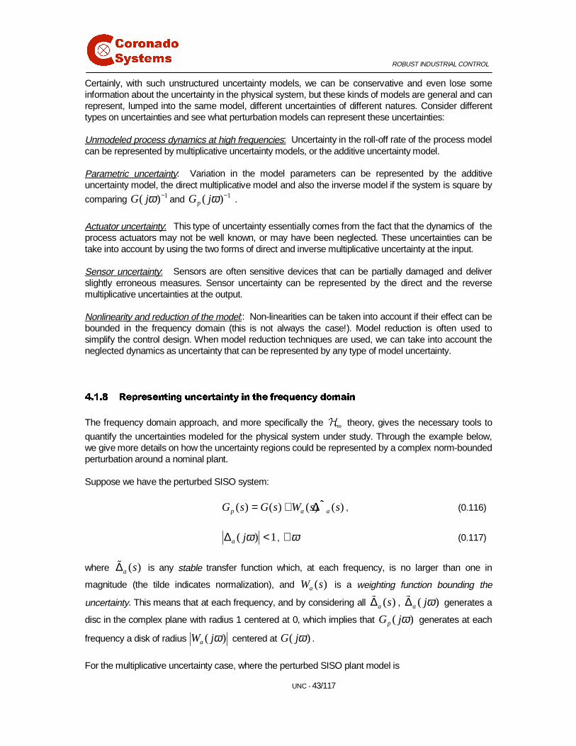
Figure 20: Covering multiplicative uncertainty with a weighting function
The dotted lines are the ( )mr ω . The first weighting function (first try of fitting) is:
0.2
, 4( / 2.5) 1
TsT
T s
+ =+
(0.123)
It doesn't fit very well. After a gain correction, we got a better weighting function: (The dashed line):
2
2
0.2 1.6 1
( / 2.5) 1 1.4 1Ts s s
T s s s
+ + +×+ + +
(0.124)
��� 7KHRUHPV IRU UREXVWFORVHG�ORRS VWDELOLW\ZLWK XQVWUXFWXUHGXQFHUWDLQW\
We will now discuss the stability of closed-loop systems subject to uncertainties. For each of thedifferent type of the uncertainty described above we will obtain a condition of robust stability that can beexploited.
Two approaches are used to deduce the conditions of the robust stability problem. The first is based onthe Nyquist criterion and the second one uses the “small-gain theorem”. Both of the theorems lead tothe same robust stability conditions but the required assumptions are not the same.
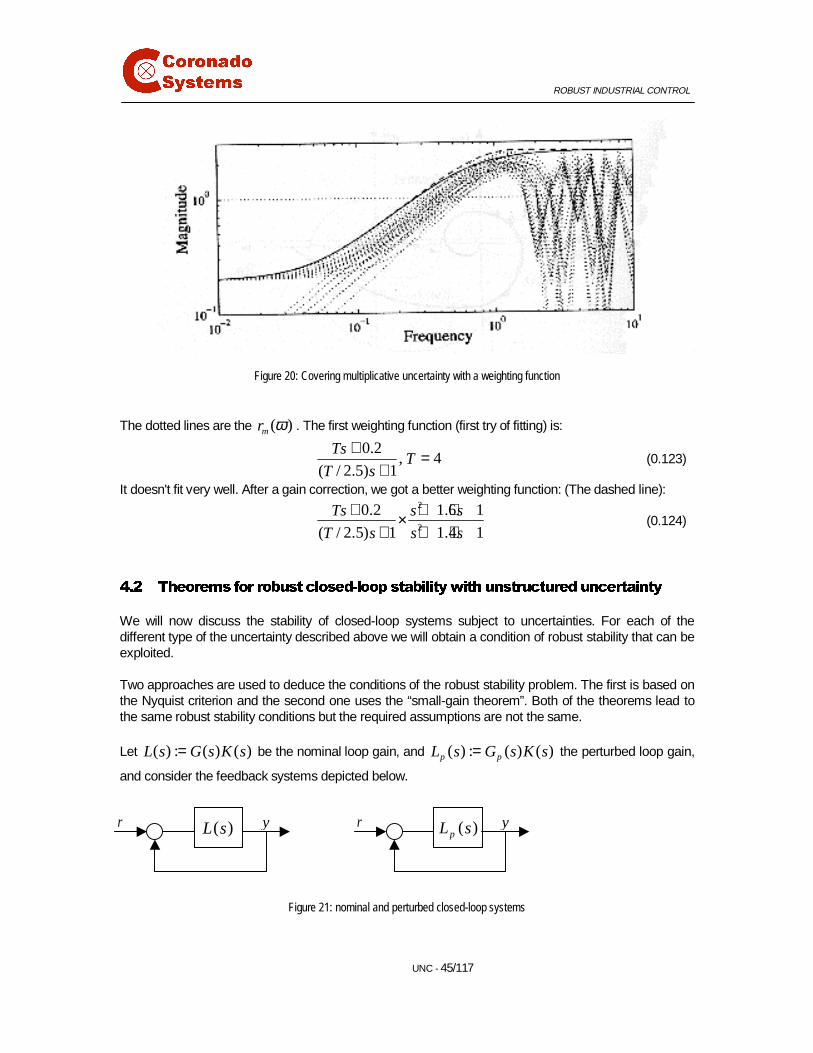
Let ( ) : ( ) ( )L s G s K s= be the nominal loop gain, and ( ) : ( ) ( )p pL s G s K s= the perturbed loop gain,
and consider the feedback systems depicted below.
Figure 21: nominal and perturbed closed-loop systems
r y r y( )L s ( )pL s

ROBUST INDUSTRIAL CONTROL
ROBSTAB - 46/117
The following theorem gives a sufficient condition for the stability of the closed-loop perturbed system.
Theorem:
Assume that the following conditions hold:
(A1)- ( )L s and ( )pL s have the same number of unstable poles (Re(s)>0).
(A2)- If ( )pL s has poles on the imaginary axis, they are also poles of ( )L s .
(A3)-The nominal closed-loop system is stable.
Then, the perturbed closed-loop system is stable if for each s belonging to the Nyquist contour and
every [0,1]ε ∈ : det[ (1 ) ( ) ( )] 0pI L s L sε ε+ − + ≠ .
Remarks
• The proof uses the Nyquist band produced by all possible perturbed loop gains.
• This theorem doesn't apply directly to practical robustness problems. Rather, it is used to provemore specific robustness conditions that can be computed using given data (nominal transfermatrices and size of uncertainty)
Another formulation for this theorem can be stated in the following way:
Under the assumptions A1, A2, A3 of the previous theorem, The perturbed system is stable if one ofthe two following conditions hold:
(C1) ω∀ ∈\ , [ ]{ }1 1( ) ( ) ( ) 1 ( ) ( ) 1p pI L j L j L j I L L Lσ ω ω ω− −
∞ + − < ⇔ + − < . (0.125)
(C2) ω∀ ∈\ , [ ]{ }1 1( ) ( ) ( ) 1 ( )( ) 1p pL j L j I L j L L I Lσ ω ω ω − −
∞ − + < ⇔ − + < . (0.126)
For the SISO case these two conditions reduce to a single condition written as:
ω∀ ∈\ , ( ) ( ) ( ) ( ) 1 ( ) ( )pG j K j G j K j G j K jω ω ω ω ω ω− < + (0.127)
This inequality, in fact, from the figure (), says that the robust stability condition is satisfied if, for eachpoint of the nominal Nyquist plot of ( ) ( )G j K jω ω , the circle of center ( ) ( )G j K jω ω and radius
( ) ( ) ( ) ( )pG j K j G j K jω ω ω ω− doesn’t contain the critical point (-1). This condition is shown in
the figure below.
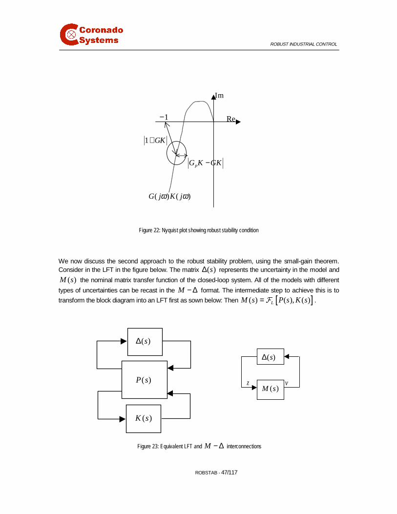
ROBUST INDUSTRIAL CONTROL
ROBSTAB - 47/117
Figure 22: Nyquist plot showing robust stability condition
We now discuss the second approach to the robust stability problem, using the small-gain theorem.Consider in the LFT in the figure below. The matrix ( )s∆ represents the uncertainty in the model and
( )M s the nominal matrix transfer function of the closed-loop system. All of the models with different
types of uncertainties can be recast in the M − ∆ format. The intermediate step to achieve this is to
transform the block diagram into an LFT first as sown below: Then [ ]( ) ( ), ( )LM s P s K s= � .
Figure 23: Equivalent LFT and M − ∆ interconnections
Im
Re
( ) ( )G j K jω ω
1 GK+
pG K GK−
( )s∆
( )M svz
1−
P s( )
( )s∆
( )K s
ROBUST INDUSTRIAL CONTROL
ROBSTAB - 48/117
Small-Gain Theorem:
Under the assumption (A4) that ( )M s and ( )s∆ are stable, i.e., ( ) , ( )M s s∞ ∞∈ ∆ ∈* * ,
the M − ∆ interconnection shown above is stable for every perturbation ( )s∆ such that 1∞∆ < iff
1M ∞ ≤ .
This theorem gives a necessary and sufficient condition for robust stability under the assumptions thatthe nominal closed-loop system ( )M s is stable, and that the uncertainty ( )s∆ is also stable and
normalized to have an ∞ -norm less than 1. The assumption that ( )s∆ be stable is not too restrictive
since such perturbations can generate unstable perturbed plant models with appropriate uncertaintymodels, such as inverse multiplicative or feedback uncertainty models.
We apply in the following subsections the robust stability theorems presented above to the varioustypes of uncertainties. For each case we’ll deduce a robust stability condition that guarantees thestability of the perturbed closed-loop system.
����� 5REXVW VWDELOLW\ZLWK DGGLWLYH XQFHUWDLQW\
Theorem
Under assumptions (A1), (A2), (A3), the closed-loop system in is stable if:
ω∀ ∈\ ,1
( ) ( ) ( ) ( ) 1a pj K j I G j K jω ω ω ω−
∆ + < . (0.128)
Under assumptions (A4), the closed-loop system in figure() is stable if and only if:
ω∀ ∈\ ,1 1( ) ( ) ( ) ( )p aK j I G j K jω ω ω δ ω
− − + ≤ (0.129)
Figure 24: Equivalent M − ∆ interconnection for additive uncertainty

ROBUST INDUSTRIAL CONTROL
ROBSTAB - 49/117
Sketch of Proof: Using the approach based on the Nyquist contour, and under assumptions (A1), (A2),(A3), the nominal and perturbed open loop matrices are given as follows:
( ) ( ) ( )L s G s K s= , (0.130)
( ) ( ) ( ) ( ( ) ( )) ( )p p aL s G s K s G s s K s= = + ∆ . (0.131)
Hence ( ) ( ) ( ) ( )p aL s L s s K s− = ∆ such that condition (C2) is equivalent to (recall that
( )Q Qσ= ):
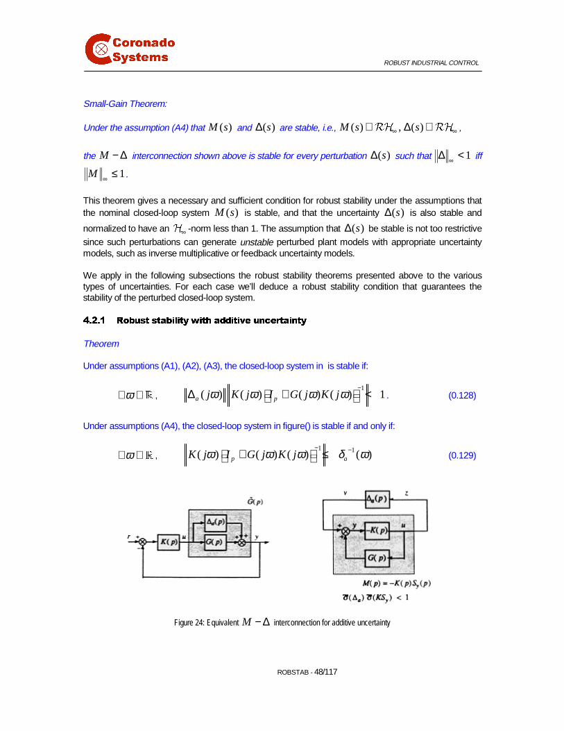
1( ( )) ( ( )( ( ) ( )) ) 1a pj K j I G j K jσ ω σ ω ω ω −∆ + < . (0.132)
Using the second approach (small-gain theorem), and under the assumption (A4), we have to put theclosed loop system in the M − ∆ form. For this we have to isolate the matrix ( )s∆ and calculate the
nominal matrix ( )M s . We obtain ( )M s by calculating the transfer matrix between the input z and
the output v of ( )s∆ . Specifically for the additive case, and in the absence of the reference signal:
1( ) ( )pz u Ky K Gz v z K I GK v−= − = − + ⇔ = − + . (0.133)
This equation correspond in fact to Figure 24. Using
[ ]( ) ( ), ( ) ( )( ( ) ( ))L pM s P s K s K s I G s K s= = − +� (0.134)
and by applying the small-gain theorem, we derive the robust stability condition given above.
Note that both approaches lead to the same robust stability condition, but the assumptions of the firstapproach are less conservative than in the second approach where ( )s∆ has to be stable.
In fact the robust stability condition for additive uncertainty can be written as :
( ( )) ( ( ) ( )) 1a yj K j S jσ ω σ ω ω∆ < where yS is the output sensitivity. In robust control design, we
have to decrease the term ( ) ( )yK j S jω ω so that the system can tolerate more additive uncertainty.

ROBUST INDUSTRIAL CONTROL
ROBSTAB - 50/117
����� 5REXVW VWDELOLW\ZLWK PXOWLSOLFDWLYH XQFHUWDLQW\
Input multiplicative uncertainty
Theorem
Under assumptions (A1), (A2), (A3), the closed-loop system in the figure below is stable if:
ω∀ ∈\ , [ ] 1( ) ( ) ( ) ( ) ( ) 1s mj K j G j I K j G jω ω ω ω ω −∆ + < , (0.135)
or, equivalently, [ ] 1 1( ) ( ) ( ) ( ) ( )m mK j G j I K j G jω ω ω ω δ ω− −+ < . (0.136)
Under assumption (A4), the closed-loop system in the figure below is stable if and only if:
ω∀ ∈\ , [ ] 1 1( ) ( ) ( ) ( ) ( )m mK j G j I K j G jω ω ω ω δ ω− −+ < . (0.137)
Figure 25: Equivalent M − ∆ interconnection for input multiplicative uncertainty
This last condition can be written as: 1( ) ( )u mT jω δ ω−< , where
[ ] 1( ) : ( ) ( ) ( ) ( )u mT s K s G s I K s G s
−= + (0.138)
is the input complementary sensitivity matrix. We can see from the robust stability condition for an inputmultiplicative uncertainty, that uT reflects the capacity of the system to tolerate uncertainty in the
actuators.


![Robust Model Predictive Control - Carnegie Mellon …cepac.cheme.cmu.edu/.../Ronust_Control_Classnotes.pdf1 Robust Model Predictive Control Formulations of robust control [1] The robust](https://img.pdfslide.net/doc/110x75/5aab45707f8b9a2b4c8bd345/robust-model-predictive-control-carnegie-mellon-cepacchemecmueduronustcontrol.jpg)