METHODSpublished: 14 August 2018

doi: 10.3389/fninf.2018.00053

Frontiers in Neuroinformatics | www.frontiersin.org 1 August 2018 | Volume 12 | Article 53

Edited by:

Isabella Castiglioni,

Istituto di Bioimmagini e Fisiologia

Molecolare (IBFM), Italy

Reviewed by:

Stavros I. Dimitriadis,

Institute of Psychological Medicine

and Clinical Neurosciences, Cardiff

University School of Medicine,

United Kingdom

Alessia Sarica,

Centro di Ricerca Neuroscientifica,

Dipartimento di Scienze Mediche e

Chirurgiche, Università degli

Studi Magna Graecia, Italy

*Correspondence:

Diego Castillo-Barnes

diegoc@ugr.es

Received: 30 April 2018

Accepted: 25 July 2018

Published: 14 August 2018

Citation:

Castillo-Barnes D, Ramírez J,

Segovia F, Martínez-Murcia FJ,

Salas-Gonzalez D and Górriz JM

(2018) Robust Ensemble Classification

Methodology for I123-Ioflupane

SPECT Images and Multiple

Heterogeneous Biomarkers in the

Diagnosis of Parkinson’s Disease.

Front. Neuroinform. 12:53.

doi: 10.3389/fninf.2018.00053

Robust Ensemble ClassificationMethodology for I123-IoflupaneSPECT Images and MultipleHeterogeneous Biomarkers in theDiagnosis of Parkinson’s DiseaseDiego Castillo-Barnes*, Javier Ramírez, Fermín Segovia, Francisco J. Martínez-Murcia,

Diego Salas-Gonzalez and Juan M. Górriz

Signal Processing and Biomedical Applications (SiPBA), Department of Signal Processing, Networking and Communications,

University of Granada, Granada, Spain

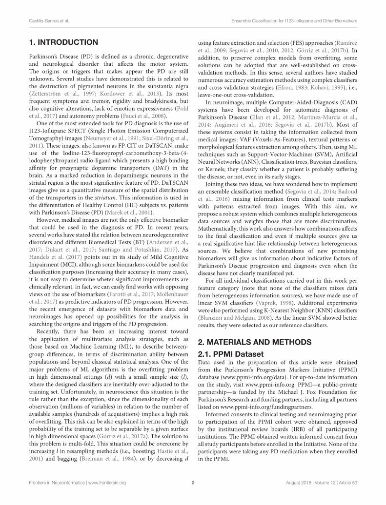
In last years, several approaches to develop an effective Computer-Aided-Diagnosis

(CAD) system for Parkinson’s Disease (PD) have been proposed. Most of these methods

have focused almost exclusively on brain images through the use of Machine-Learning

algorithms suitable to characterize structural or functional patterns. Those patterns

provide enough information about the status and/or the progression at intermediate

and advanced stages of Parkinson’s Disease. Nevertheless this information could be

insufficient at early stages of the pathology. The Parkinson’s ProgressionMarkers Initiative

(PPMI) database includes neurological images along with multiple biomedical tests.

This information opens up the possibility of comparing different biomarker classification

results. As data come from heterogeneous sources, it is expected that we could include

some of these biomarkers in order to obtain new information about the pathology. Based

on that idea, this work presents an Ensemble Classification model with Performance

Weighting. This proposal has been tested comparing Healthy Control subjects (HC)

vs. patients with PD (considering both PD and SWEDD labeled subjects as the same

class). This model combines several Support-Vector-Machine (SVM) with linear kernel

classifiers for different biomedical group of tests—including CerebroSpinal Fluid (CSF),

RNA, and Serum tests—and pre-processed neuroimages features (Voxels-As-Features

and a list of definedMorphological Features) fromPPMI database subjects. The proposed

methodology makes use of all data sources and selects the most discriminant features

(mainly from neuroimages). Using this performance-weighted ensemble classification

model, classification results up to 96% were obtained.

Keywords: Machine Learning, ensemble, SVM (Support-Vector-Machine), Parkinson’s Disease, SPECT (Single

Photon Emission Computerized Tomography), biomarkers, PPMI (Parkinson’s Progression Markers Initiative)

Castillo-Barnes et al. Ensemble Classification for I123-Ioflupane and Other Biomarkers

1. INTRODUCTION

Parkinson’s Disease (PD) is defined as a chronic, degenerativeand neurological disorder that affects the motor system.The origins or triggers that makes appear the PD are stillunknown. Several studies have demonstrated this is related tothe destruction of pigmented neurons in the substantia nigra(Zetterström et al., 1997; Kordower et al., 2013). Its mostfrequent symptoms are: tremor, rigidity and bradykinesia, butalso cognitive alterations, lack of emotion expressiveness (Pohlet al., 2017) and autonomy problems (Fauci et al., 2008).

One of the most extended tools for PD diagnosis is the use ofI123-Ioflupane SPECT (Single Photon Emission ComputerizedTomography) images (Neumeyer et al., 1991; Sixel-Döring et al.,2011). These images, also known as FP-CIT or DaTSCAN, makeuse of the Iodine-123-fluoropropyl-carbomethoxy-3-beta-(4-iodophenyltropane) radio-ligand which presents a high bindingaffinity for presynaptic dopamine transporters (DAT) in thebrain. As a marked reduction in dopaminergic neurons in thestriatal region is the most significative feature of PD, DaTSCANimages give us a quantitative measure of the spatial distributionof the transporters in the striatum. This information is used inthe differentiation of Healthy Control (HC) subjects vs. patientswith Parkinson’s Disease (PD) (Marek et al., 2001).

However, medical images are not the only effective biomarkerthat could be used in the diagnosis of PD. In recent years,several works have stated the relation between neurodegenerativedisorders and different Biomedical Tests (BT) (Andersen et al.,2017; Dukart et al., 2017; Santiago and Potashkin, 2017). AsHandels et al. (2017) points out in its study of Mild CognitiveImpairment (MCI), although some biomarkers could be used forclassification purposes (increasing their accuracy in many cases),it is not easy to determine wheter significant improvements areclinically relevant. In fact, we can easily find works with opposingviews on the use of biomarkers (Farotti et al., 2017; Mollenhaueret al., 2017) as predictive indicators of PD progression. However,the recent emergence of datasets with biomarkers data andneuroimages has opened up possibilities for the analysis insearching the origins and triggers of the PD progression.

Recently, there has been an increasing interest toward

the application of multivariate analysis strategies, such asthose based on Machine Learning (ML), to describe between-

group differences, in terms of discrimination ability betweenpopulations and beyond classical statistical analysis. One of the

major problems of ML algorithms is the overfitting problemin high dimensional settings (d) with a small sample size (l),where the designed classifiers are inevitably over-adjusted to thetraining set. Unfortunately, in neuroscience this situation is therule rather than the exception, since the dimensionality of eachobservation (millions of variables) in relation to the number ofavailable samples (hundreds of acquisitions) implies a high riskof overfitting. This risk can be also explained in terms of the highprobability of the training set to be separable by a given surfacein high dimensional spaces (Górriz et al., 2017a). The solution tothis problem is multi-fold. This situation could be overcome byincreasing l in resampling methods (i.e., boosting; Hastie et al.,2001) and bagging (Breiman et al., 1984), or by decreasing d

using feature extraction and selection (FES) approaches (Ramírezet al., 2009; Segovia et al., 2010, 2012; Górriz et al., 2017b). Inaddition, to preserve complex models from overfitting, somesolutions can be adopted that are well-established on cross-validation methods. In this sense, several authors have studiednumerous accuracy estimationmethods using complex classifiersand cross-validation strategies (Efron, 1983; Kohavi, 1995), i.e.,leave-one-out cross-validation.

In neuroimage, multiple Computer-Aided-Diagnosis (CAD)systems have been developed for automatic diagnosis ofParkinson’s Disease (Illan et al., 2012; Martinez-Murcia et al.,2014; Augimeri et al., 2016; Segovia et al., 2017b). Most ofthese systems consist in taking the information collected frommedical images: VAF (Voxels-As-Features), textural patterns ormorphological features extraction among others. Then, usingMLtechniques such as Support-Vector-Machines (SVM), ArtificialNeural Networks (ANN), Classification trees, Bayesian classifiers,or Kernels; they classify whether a patient is probably sufferingthe disease, or not, even in its early stages.

Joining these two ideas, we have wondered how to implementan ensemble classification method (Segovia et al., 2014; Badoudet al., 2016) mixing information from clinical tests markerswith patterns extracted from images. With this aim, wepropose a robust system which combines multiple heterogeneousdata sources and weights those that are more discriminative.Mathematically, this work also answers how combinations affectsto the final classification and even if multiple sources give usa real significative hint like relationship between heterogeneoussources. We believe that combinations of new promisingbiomarkers will give us information about indicative factors ofParkinson’s Disease progression and diagnosis even when thedisease have not clearly manifested yet.

For all individual classifications carried out in this work perfeature category (note that none of the classifiers mixes datafrom heterogeneous information sources), we have made use oflinear SVM classifiers (Vapnik, 1998). Additional experimentswere also performed using K-Nearest Neighbor (KNN) classifiers(Blanzieri and Melgani, 2008). As the linear SVM showed betterresults, they were selected as our reference classifiers.

2. MATERIALS AND METHODS

2.1. PPMI DatasetData used in the preparation of this article were obtainedfrom the Parkinson’s Progression Markers Initiative (PPMI)database (www.ppmi-info.org/data). For up-to-date informationon the study, visit www.ppmi-info.org. PPMI—a public-privatepartnership—is funded by the Michael J. Fox Foundation forParkinson’s Research and funding partners, including all partnerslisted on www.ppmi-info.org/fundingpartners.

Informed consents to clinical testing and neuroimaging priorto participation of the PPMI cohort were obtained, approvedby the institutional review boards (IRB) of all participatinginstitutions. The PPMI obtained written informed consent fromall study participants before enrolled in the Initiative. None of theparticipants were taking any PD medication when they enrolledin the PPMI.

Frontiers in Neuroinformatics | www.frontiersin.org 2 August 2018 | Volume 12 | Article 53

Castillo-Barnes et al. Ensemble Classification for I123-Ioflupane and Other Biomarkers

TABLE 1 | Demographics.

Subjects Number Sex [Male—Female] Age [Mean (Std)]

HC 194 129—65 53.04 (2.27)

PD 168 103—65 53.14 (2.37)

SWEDD 26 17—9 53.21 (2.30)

The inclusion criteria adopted in the PPMI cohort studyare available in http://www.ppmi-info.org/wp-content/uploads/2014/06/PPMI-Amendment-8-Protocol.pdf. This diagnosticalprocedure also includes a confirmation step based on imaging butthis is not the only test to label a subject. To avoid the possiblecircularity in results, we have decided not to compare only HCvs. PD patients in our study but HC vs. non-HC subjects instead.

2.2. Demographics and DescriptiveStatistics of ParticipantsFor this work, we have retrospectively selected the baseline(BL) data available of 388 participants in the PPMI cohortstudy including Healthy Control subjects (HC), patients withParkinson’s Disease (PD) and those with PD whose scans haveno evidence of dopaminergic deficit (SWEDD) (Wyman-Chicket al., 2016). As SWEDD and PD subjects are both considered aspatients with Parkinson’s Disease, we have included both of themin the same group (PD+SWEDD).

Demographics of all participants have been included inTable 1.

2.3. Image Preprocessing2.3.1. Spatial NormalizationAll DaTSCAN images have been spatially registered usingthe SPM (Statistical Parametric Mapping) tool. Specifically,for this work, we have used the SPM12 software packageavailable from: www.fil.ion.ucl.ac.uk/spm/software/spm12/. Itsdocumentation and manuals are also available from this website.Once registration was performed, it was checked that matchingbetween voxels and anatomical structures was unaltered. Afterbeing co-registered and averaged, each cerebral image wasreoriented into a standard image grid. Obtained images had adimension of 79× 95× 78 voxels and a voxel size of 2.0× 2.0×2.0 mm.

2.3.2. Intensity NormalizationFull dataset from the PPMI was used to normalize intensity ofeach image. An intensity normalization method based on the α-Stable distributions as described in Salas-Gonzalez et al. (2009),Castillo-Barnes et al. (2017) was used for that. This approach hasshown itself to be more effective for homogenizing informationfrom SPECT images than other approaches, like the currentlywidely used intensity normalization based on Binding Ratio orthe equivalent Gaussian model, as was demonstrated in Salas-Gonzalez et al. (2013).

Mathematically, intensity normalization based on α-Stabledistributions uses a linear transformation as presented inexpression (1) with a and b as follows in (2):

Y = aX + b (1)

a =γ ∗

γb = µ∗ −

γ ∗

γµ (2)

where γ ∗ and µ∗ represent the mean of γ (dispersion) and µ

(location) parameters, respectively, that are computed for thewhole database.

In short, steps to perform intensity normalization using theα-Stable distribution schema can be summarized as follows:

• Step 1: A mask is applied to source images in order to consideronly voxels in the brain outside the striatum (Brahim et al.,2015). This will reduce the computational load without losingtoo much accuracy.

• Step 2: For each image, we compute the histogram of selectedvoxels in the previous step and fit an α-Stable distribution. Weobtain α, β , γ , and δ parameters of each image.

• Step 3: Once having all the α-Stable distributions, calculate theγ ∗ and δ∗ parameters as mean of all γ and δ parameters.

• Step 4: Get a and b values following expression (2).• Step 5: Apply the linear transformation presented in (1).

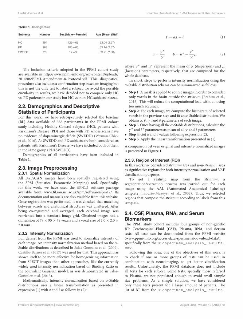
A comparison between original and intensity-normalized imagesis presented in Figure 1.

2.3.3. Region of Interest (ROI)In this work, we considered striatum area and non-striatum areaas significative regions for both intensity normalization and VAFclassification purposes.

To get a realistic map from the striatum, asegmentation/extraction process was carried out for eachimage using the AAL (Automated Anatomical Labeling)template (Tzourio-Mazoyer et al., 2002). Thus, we selectedregions that compose the striatum according to labels from thistemplate.

2.4. CSF, Plasma, RNA, and SerumBiomarkersThe PPMI study cohort includes four groups of non-geneticBT: Cerebrospinal-Fluid (CSF), Plasma, RNA, and Serum

tests. All tests can be downloaded from the PPMI website(www.ppmi-info.org/access-data-specimens/download-data/),specifically from the Biospecimen_Analysis_Results.csv.

Following this idea, one of the objectives of this work isto check if one or more groups of tests can be used, incombination with neuroimaging, to get better classificationresults. Unfortunately, the PPMI database does not includeall tests for each subject. Some tests, specially those referredto Plasma, are not populated enough to avoid small samplesize problems. As a simple solution, we have consideredonly these tests present for a large amount of patients. Thelist of BT from the Biospecimen_Analysis_Results.

Frontiers in Neuroinformatics | www.frontiersin.org 3 August 2018 | Volume 12 | Article 53

Castillo-Barnes et al. Ensemble Classification for I123-Ioflupane and Other Biomarkers

FIGURE 1 | Comparison between intensity normalizated images using the α-Stable normalization procedure (Up) and their respective original versions (Down).

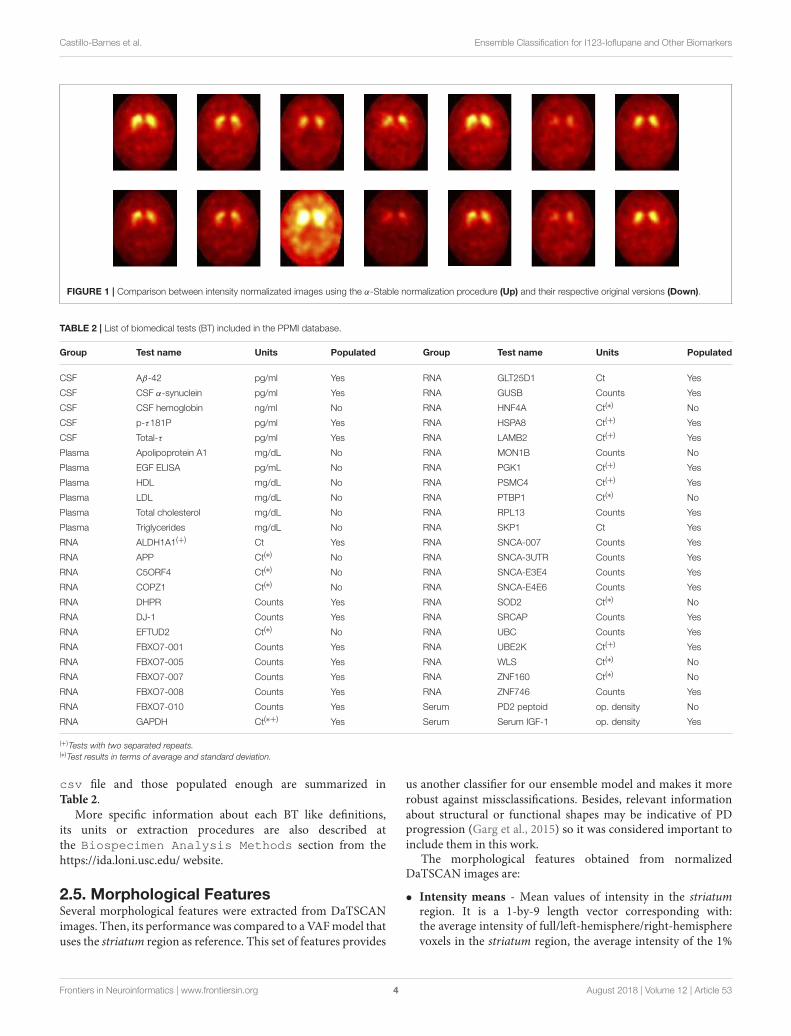
TABLE 2 | List of biomedical tests (BT) included in the PPMI database.

Group Test name Units Populated Group Test name Units Populated

CSF Aβ-42 pg/ml Yes RNA GLT25D1 Ct Yes

CSF CSF α-synuclein pg/ml Yes RNA GUSB Counts Yes

CSF CSF hemoglobin ng/ml No RNA HNF4A Ct(∗) No

CSF p-τ181P pg/ml Yes RNA HSPA8 Ct(+) Yes

CSF Total-τ pg/ml Yes RNA LAMB2 Ct(+) Yes

Plasma Apolipoprotein A1 mg/dL No RNA MON1B Counts No

Plasma EGF ELISA pg/mL No RNA PGK1 Ct(+) Yes

Plasma HDL mg/dL No RNA PSMC4 Ct(+) Yes

Plasma LDL mg/dL No RNA PTBP1 Ct(∗) No

Plasma Total cholesterol mg/dL No RNA RPL13 Counts Yes

Plasma Triglycerides mg/dL No RNA SKP1 Ct Yes

RNA ALDH1A1(+) Ct Yes RNA SNCA-007 Counts Yes

RNA APP Ct(∗) No RNA SNCA-3UTR Counts Yes

RNA C5ORF4 Ct(∗) No RNA SNCA-E3E4 Counts Yes

RNA COPZ1 Ct(∗) No RNA SNCA-E4E6 Counts Yes

RNA DHPR Counts Yes RNA SOD2 Ct(∗) No

RNA DJ-1 Counts Yes RNA SRCAP Counts Yes

RNA EFTUD2 Ct(∗) No RNA UBC Counts Yes

RNA FBXO7-001 Counts Yes RNA UBE2K Ct(+) Yes

RNA FBXO7-005 Counts Yes RNA WLS Ct(∗) No

RNA FBXO7-007 Counts Yes RNA ZNF160 Ct(∗) No

RNA FBXO7-008 Counts Yes RNA ZNF746 Counts Yes

RNA FBXO7-010 Counts Yes Serum PD2 peptoid op. density No

RNA GAPDH Ct(∗+) Yes Serum Serum IGF-1 op. density Yes

(+)Tests with two separated repeats.(∗)Test results in terms of average and standard deviation.

csv file and those populated enough are summarized inTable 2.

More specific information about each BT like definitions,its units or extraction procedures are also described atthe Biospecimen Analysis Methods section from thehttps://ida.loni.usc.edu/ website.

2.5. Morphological FeaturesSeveral morphological features were extracted from DaTSCANimages. Then, its performance was compared to a VAFmodel thatuses the striatum region as reference. This set of features provides

us another classifier for our ensemble model and makes it morerobust against missclassifications. Besides, relevant informationabout structural or functional shapes may be indicative of PDprogression (Garg et al., 2015) so it was considered important toinclude them in this work.

The morphological features obtained from normalizedDaTSCAN images are:

• Intensity means - Mean values of intensity in the striatumregion. It is a 1-by-9 length vector corresponding with:the average intensity of full/left-hemisphere/right-hemispherevoxels in the striatum region, the average intensity of the 1%

Frontiers in Neuroinformatics | www.frontiersin.org 4 August 2018 | Volume 12 | Article 53

Castillo-Barnes et al. Ensemble Classification for I123-Ioflupane and Other Biomarkers

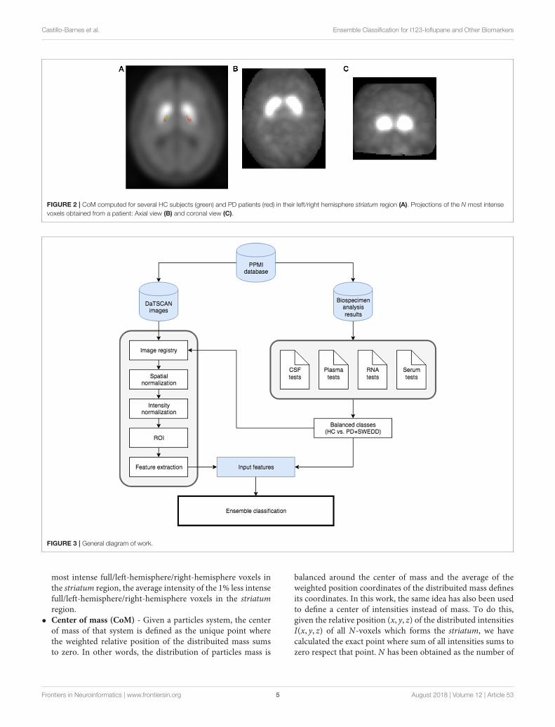
FIGURE 2 | CoM computed for several HC subjects (green) and PD patients (red) in their left/right hemisphere striatum region (A). Projections of the N most intense

voxels obtained from a patient: Axial view (B) and coronal view (C).

FIGURE 3 | General diagram of work.

most intense full/left-hemisphere/right-hemisphere voxels inthe striatum region, the average intensity of the 1% less intensefull/left-hemisphere/right-hemisphere voxels in the striatumregion.

• Center of mass (CoM) - Given a particles system, the centerof mass of that system is defined as the unique point wherethe weighted relative position of the distribuited mass sumsto zero. In other words, the distribution of particles mass is

balanced around the center of mass and the average of theweighted position coordinates of the distribuited mass definesits coordinates. In this work, the same idea has also been usedto define a center of intensities instead of mass. To do this,given the relative position (x, y, z) of the distributed intensitiesI(x, y, z) of all N-voxels which forms the striatum, we havecalculated the exact point where sum of all intensities sums tozero respect that point. N has been obtained as the number of

Frontiers in Neuroinformatics | www.frontiersin.org 5 August 2018 | Volume 12 | Article 53

Castillo-Barnes et al. Ensemble Classification for I123-Ioflupane and Other Biomarkers

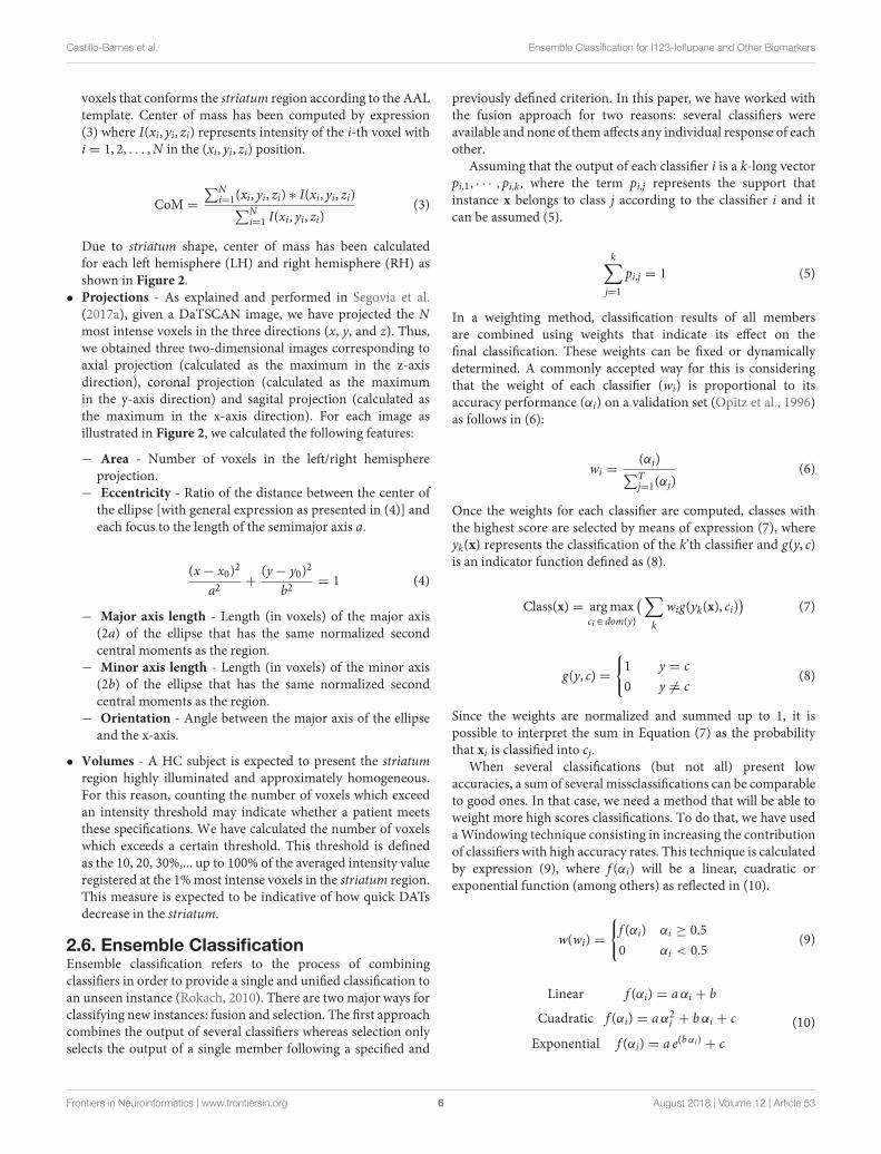
voxels that conforms the striatum region according to the AALtemplate. Center of mass has been computed by expression(3) where I(xi, yi, zi) represents intensity of the i-th voxel withi = 1, 2, . . . ,N in the (xi, yi, zi) position.

CoM =

∑Ni=1(xi, yi, zi) ∗ I(xi, yi, zi)

∑Ni=1 I(xi, yi, zi)

(3)

Due to striatum shape, center of mass has been calculatedfor each left hemisphere (LH) and right hemisphere (RH) asshown in Figure 2.

• Projections - As explained and performed in Segovia et al.(2017a), given a DaTSCAN image, we have projected the Nmost intense voxels in the three directions (x, y, and z). Thus,we obtained three two-dimensional images corresponding toaxial projection (calculated as the maximum in the z-axisdirection), coronal projection (calculated as the maximumin the y-axis direction) and sagital projection (calculated asthe maximum in the x-axis direction). For each image asillustrated in Figure 2, we calculated the following features:

− Area - Number of voxels in the left/right hemisphereprojection.

− Eccentricity - Ratio of the distance between the center ofthe ellipse [with general expression as presented in (4)] andeach focus to the length of the semimajor axis a.

(x− x0)2

a2+

(y− y0)2

b2= 1 (4)

− Major axis length - Length (in voxels) of the major axis(2a) of the ellipse that has the same normalized secondcentral moments as the region.

− Minor axis length - Length (in voxels) of the minor axis(2b) of the ellipse that has the same normalized secondcentral moments as the region.

− Orientation - Angle between the major axis of the ellipseand the x-axis.

• Volumes - A HC subject is expected to present the striatumregion highly illuminated and approximately homogeneous.For this reason, counting the number of voxels which exceedan intensity threshold may indicate whether a patient meetsthese specifications. We have calculated the number of voxelswhich exceeds a certain threshold. This threshold is definedas the 10, 20, 30%,... up to 100% of the averaged intensity valueregistered at the 1%most intense voxels in the striatum region.This measure is expected to be indicative of how quick DATsdecrease in the striatum.

2.6. Ensemble ClassificationEnsemble classification refers to the process of combiningclassifiers in order to provide a single and unified classification toan unseen instance (Rokach, 2010). There are two major ways forclassifying new instances: fusion and selection. The first approachcombines the output of several classifiers whereas selection onlyselects the output of a single member following a specified and

previously defined criterion. In this paper, we have worked withthe fusion approach for two reasons: several classifiers wereavailable and none of them affects any individual response of eachother.

Assuming that the output of each classifier i is a k-long vectorpi,1, · · · , pi,k, where the term pi,j represents the support thatinstance x belongs to class j according to the classifier i and itcan be assumed (5).

k∑

j=1

pi,j = 1 (5)

In a weighting method, classification results of all membersare combined using weights that indicate its effect on thefinal classification. These weights can be fixed or dynamicallydetermined. A commonly accepted way for this is consideringthat the weight of each classifier (wi) is proportional to itsaccuracy performance (αi) on a validation set (Opitz et al., 1996)as follows in (6):

wi =(αi)

∑Tj=1(αj)

(6)

Once the weights for each classifier are computed, classes withthe highest score are selected by means of expression (7), whereyk(x) represents the classification of the k’th classifier and g(y, c)is an indicator function defined as (8).

Class(x) = argmaxci ∈ dom(y)

(

∑

k

wig(yk(x), ci))

(7)

g(y, c) =

{

1 y = c

0 y 6= c(8)

Since the weights are normalized and summed up to 1, it ispossible to interpret the sum in Equation (7) as the probabilitythat xi is classified into cj.

When several classifications (but not all) present lowaccuracies, a sum of several missclassifications can be comparableto good ones. In that case, we need a method that will be able toweight more high scores classifications. To do that, we have usedaWindowing technique consisting in increasing the contributionof classifiers with high accuracy rates. This technique is calculatedby expression (9), where f (αi) will be a linear, cuadratic orexponential function (among others) as reflected in (10).

w(wi) =

{

f (αi) αi ≥ 0.5

0 αi < 0.5(9)

Linear f (αi) = aαi + b

Cuadratic f (αi) = aα2i + bαi + c

Exponential f (αi) = a e(bαi) + c

(10)

Frontiers in Neuroinformatics | www.frontiersin.org 6 August 2018 | Volume 12 | Article 53

Castillo-Barnes et al. Ensemble Classification for I123-Ioflupane and Other Biomarkers

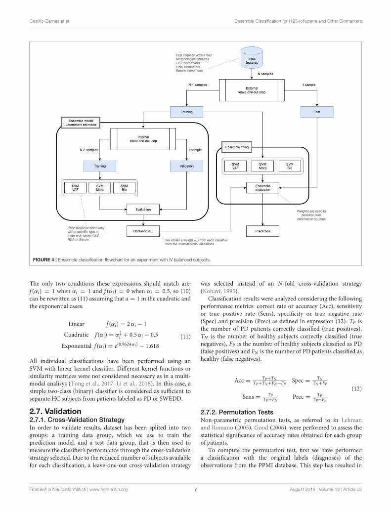
FIGURE 4 | Ensemble classification flowchart for an experiment with N balanced subjects.

The only two conditions these expressions should match are:f (αi) = 1 when αi = 1 and f (αi) = 0 when αi = 0.5, so (10)can be rewritten as (11) assuming that a = 1 in the cuadratic andthe exponential cases.

Linear f (αi) = 2αi − 1

Cuadratic f (αi) = α2i + 0.5αi − 0.5

Exponential f (αi) = e(0.9624αi) − 1.618

(11)

All individual classifications have been performed using anSVM with linear kernel classifier. Different kernel functions orsimilarity matrices were not considered necessary as in a multi-modal analisys (Tong et al., 2017; Li et al., 2018). In this case, asimple two-class (binary) classifier is considered as sufficient toseparate HC subjects from patients labeled as PD or SWEDD.

2.7. Validation2.7.1. Cross-Validation StrategyIn order to validate results, dataset has been splited into twogroups: a training data group, which we use to train theprediction model, and a test data group, that is then used tomeasure the classifier’s performance through the cross-validationstrategy selected. Due to the reduced number of subjects availablefor each classification, a leave-one-out cross-validation strategy

was selected instead of an N-fold cross-validation strategy(Kohavi, 1995).

Classification results were analyzed considering the followingperformance metrics: correct rate or accuracy (Acc), sensitivityor true positive rate (Sens), specificity or true negative rate(Spec) and precision (Prec) as defined in expression (12). TP isthe number of PD patients correctly classified (true positives),TN is the number of healthy subjects correctly classified (truenegatives), FP is the number of healthy subjects classified as PD(false positives) and FN is the number of PD patients classified ashealthy (false negatives).

Acc = TP+TNTP+TN+FN+FP

Spec = TNTN+FP

Sens = TPTP+FN

Prec = TPTP+FP

(12)

2.7.2. Permutation TestsNon-parametric permutation tests, as referred to in Lehmanand Romano (2005), Good (2006), were performed to assess thestatistical significance of accuracy rates obtained for each groupof patients.

To compute the permutation test, first we have performeda classification with the original labels (diagnoses) of theobservations from the PPMI database. This step has resulted in

Frontiers in Neuroinformatics | www.frontiersin.org 7 August 2018 | Volume 12 | Article 53

Castillo-Barnes et al. Ensemble Classification for I123-Ioflupane and Other Biomarkers

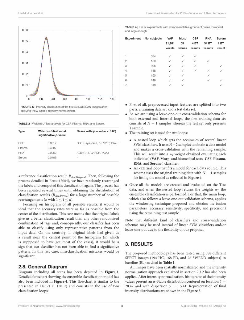
FIGURE 5 | Intensity distribution of the first 50 DaTSCAN images after

applying the α-Stable intensity normalization.

TABLE 3 | Welch’s U-Test analysis for CSF, Plasma, RNA, and Serum.

Type Welch’s U-Test most

significative p-value

Cases with (p− value < 0.05)

CSF 0.0017 CSF α-synuclein, p-τ181P, Total-τ

Plasma 0.4887 -

RNA 0.0052 ALDH1A1, GAPDH, PGK1

Serum 0.0756 -

a reference classification result: RAcc,Original. Then, following theprocess detailed in Ernst (2004), we have randomly rearrangedthe labels and computed this classification again. The process hasbeen repeated several times until obtaining the distribution ofclassification results (RAcc,Permi ) for a large number of possiblerearrangements (n with 1 ≤ i ≤ n).

Focusing on histogram of all possible results, it would beideal that the accuracy rates were as far as possible from thecenter of the distribution. This case means that the original labelsgive us a better classification result than any other randomizedcombination of tags and, consequently, our classifier has beenable to classify using only representative patterns from theinput data. On the contrary, if original labels had given usa result near the central point of the histogram (in whichis suppposed to have got most of the cases), it would be asign that our classifier has not been able to find a significativepattern. In this last case, missclassification mistakes would besignificant.

2.8. General DiagramDiagram including all steps has been depicted in Figure 3.Detailed flowchart showing the ensemble classificationmodel hasalso been included in Figure 4. This flowchart is similar to thepresented in Dai et al. (2012) and consists in the use of twoclassification loops:

TABLE 4 | List of experiments with all representative groups of cases, balanced,

and large enough.

Experiment No. subjects VAF Morp CSF RNA Serum

21,981 55 4 BT 34 BT 1 BT

voxels values results results result

1 334 X X X

2 150 X X X X

3 306 X X X X

4 148 X X X X X

5 150 X X X

6 148 X X X X

7 310 X X X

• First of all, preprocessed input features are splitted into twoparts: a training data set and a test data set.

• As we are using a leave-one-out cross-validation schema forboth external and internal loops, the first training data setconsists of N − 1 samples whereas the test set only presents1 sample.

• The training set is used for two loops:

• A nested loop which gets the accuracies of several linearSVM classifiers. It usesN−2 samples to obtain a data modeland makes a cross-validation with the remaining sample.This will result into a wi weight obtained evaluating eachindividual (VAF,Morp, and biomedical tests -CSF, Plasma,RNA, and Serum-) classifier.

• An external loop that fits a model for each data source. Thisschema uses the original training data with N − 1 samplesfor fitting the model as reflected in Figure 4.

• Once all the models are created and evaluated on the Testdata, and when the nested loop returns the weights wi, theensemble classification is performed. For that, the main loop,which also follows a leave-one-out validation schema, appliesthe windowing technique proposed and obtains the fusionparameters (accuracy, sensitivity, specificity, and precision)using the remaining test sample.

Note that different kind of classifiers and cross-validationschemas may be used instead of linear SVM classifiers and/orleave-one-out due to the flexibility of our proposal.

3. RESULTS

The proposed methodology has been tested using 388 differentSPECT images (194 HC, 168 PD, and 26 SWEDD subjects) inbaseline (BL) as cited in Table 1.

All images have been spatially normalizated and the intensitynormalization approach explained in section 2.3.2 has also beenapplied. After intensity normalization, histograms of the intensityvalues present an α-Stable distribution centered on location δ =

28.42 and with dispersion γ = 5.41. Representation of finalintensity distributions are shown in the Figure 5.

Frontiers in Neuroinformatics | www.frontiersin.org 8 August 2018 | Volume 12 | Article 53

Castillo-Barnes et al. Ensemble Classification for I123-Ioflupane and Other Biomarkers

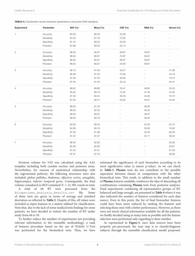
TABLE 5 | Classification results (individual classifications using linear SVM classifiers).

Experiment Parameter VAF (%) Morp (%) CSF (%) RNA (%) Serum (%)

1 Accuracy 82.93 88.32 52.99 - -

Sensitivity 84.43 87.43 73.05 - -

Specificity 81.44 89.22 32.93 - -

Precision 81.98 89.02 52.14 - -

2 Accuracy 96.00 90.67 56.67 58.67 -

Sensitivity 96.00 90.67 74.67 58.67 -

Specificity 96.00 90.67 38.67 58.67 -

Precision 96.00 90.67 54.90 58.67 -

3 Accuracy 96.73 91.50 53.27 - 51.96

Sensitivity 96.08 91.50 70.59 - 24.18

Specificity 97.39 91.50 35.95 - 79.74

Precision 97.35 91.50 52.43 - 54.41

4 Accuracy 96.62 89.86 55.41 48.65 52.03

Sensitivity 95.95 89.19 74.32 47.30 24.32

Specificity 97.30 90.54 36.49 50.00 79.73

Precision 97.26 90.41 53.92 48.61 54.55

5 Accuracy 96.00 91.33 - 48.00 -

Sensitivity 96.00 92.00 - 49.33 -

Specificity 96.00 90.67 - 46.67 -

Precision 96.00 90.79 - 48.05 -

6 Accuracy 95.95 90.54 - 52.03 52.70

Sensitivity 94.59 89.19 - 50.00 18.92

Specificity 97.30 91.89 - 54.05 86.49

Precision 97.22 91.67 - 52.11 58.33

7 Accuracy 96.45 92.26 - - 52.58

Sensitivity 95.48 92.90 - - 23.87

Specificity 97.42 91.61 - - 81.29

Precision 97.37 91.72 - - 56.06

Striatum volume for VAF was calculated using the AALtemplate including both caudate nucleus and putamen areas.Nevertheless, for reasons of anatomical relationship withthe nigrostriatal pathway, the following structures were alsoincluded: globus pallidus, thalamus, olfactory cortex, amygdala,hippocampus, inferior temporal gyrus. Consequently, the finalvolume considered as ROI contained N = 21, 981 voxels in total.

A total of 68 BT were processed from theBiospecimen_Analysis_Results.csv file. Someof these tests are given in terms of average and standarddesviation as reflected in Table 2. Despite of this, all values wereincluded as input features in a matrix utilized for classification.Note that, due to the lack of some medical tests findings for somepatients, we have decided to restrict the number of BT understudy from 68 to 39.

To further reduce the number of experiments not providingrelevant information to the ensemble methodology, a rankof features procedure based on the use of Welch’s U-Testwas performed for the biomedical tests. Thus, we have

estimated the significance of each biomarker according to itsmost significative value (a minor p-value). As we can checkin Table 3, Plasma tests do not contribute to the possibleseparation between classes in comparisson with the otherbiomedical tests. This result, in addition to the small numberof Plasma features available, reinforces the idea of discarding allcombinations containing Plasma tests from posterior analyses.Final experiments combining all representative groups of BT,balanced and large enough, are presented in Table 4 where it wasalso indicated the number of features considered for each datasource. Even in this point, the list of final biomarker featurescould have been more reduced by ranking the features andselecting those ones with a better performance. However, as therewere not much clinical information available for all the patients,we finally decided using as many tests as possible and the featureselection were performed only regarding to their number.

As represented in Figure 3, once data sources have beenproperly pre-processed, the next step is to classify/diagnosesubjects through the ensemble classification model proposed.

Frontiers in Neuroinformatics | www.frontiersin.org 9 August 2018 | Volume 12 | Article 53

Castillo-Barnes et al. Ensemble Classification for I123-Ioflupane and Other Biomarkers

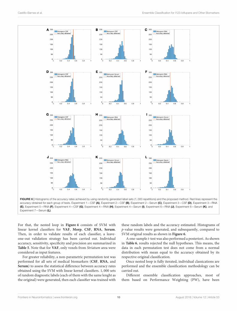
FIGURE 6 | Histograms of the accuracy rates achieved by using randomly generated label sets (1, 000 repetitions) and the proposed method. Red lines represent the

accuracy obtained for each group of tests. Experiment 1—CSF (A), Experiment 2—CSF (B), Experiment 2—Serum (C), Experiment 3—CSF (D), Experiment 3—RNA

(E), Experiment 5—RNA (F), Experiment 4—CSF (G), Experiment 4—RNA (H), Experiment 4—Serum (I), Experiment 6—RNA (J), Experiment 6—Serum (K), and

Experiment 7—Serum (L).

For that, the nested loop in Figure 4 consists of SVM withlinear kernel classifiers for VAF, Morp, CSF, RNA, Serum.Then, in order to validate results of each classifier, a leave-one-out validation strategy has been carried out. Individualaccuracy, sensitivity, specificity and precision are summarized inTable 5. Note that for VAF, only voxels from Striatum area wereconsidered as input features.

For greater reliability, a non-parametric permutation test wasperformed for all sets of medical biomarkers (CSF, RNA, andSerum) to assess the statistical difference between accuracy ratesobtained using the SVM with linear kernel classifiers. 1, 000 setsof random diagnostic labels (each of themwith the same lenght asthe original) were generated, then each classifier was trained with

these random labels and the accuracy estimated. Histograms ofp-value results were generated, and subsequently, compared toSVM original results as shown in Figure 6.

A one-sample t-test was also performed a posteriori. As shownin Table 6, results rejected the null hypotheses. This means, thedata in each permutation test does not come from a normaldistribution with mean equal to the accuracy obtained by itsrespective original classification.

Once nested loop is fully iterated, individual classications areperformed and the ensemble classification methodology can becarried out.

Different ensemble classification approaches, most ofthem based on Performance Weighting (PW), have been

Frontiers in Neuroinformatics | www.frontiersin.org 10 August 2018 | Volume 12 | Article 53

Castillo-Barnes et al. Ensemble Classification for I123-Ioflupane and Other Biomarkers

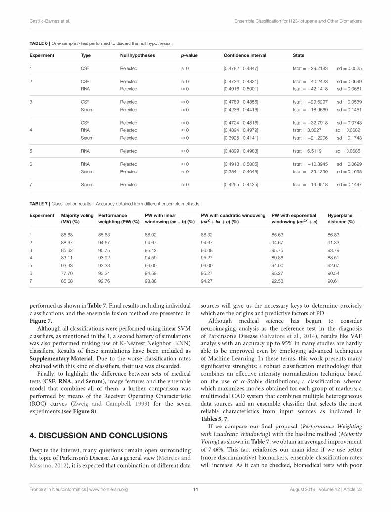
TABLE 6 | One-sample t-Test performed to discard the null hypotheses.

Experiment Type Null hypotheses p-value Confidence interval Stats

1 CSF Rejected ≈ 0 [0.4782 , 0.4847] tstat = −29.2183 sd = 0.0525

2 CSF Rejected ≈ 0 [0.4734 , 0.4821] tstat = −40.2423 sd = 0.0699

RNA Rejected ≈ 0 [0.4916 , 0.5001] tstat = −42.1418 sd = 0.0681

3 CSF Rejected ≈ 0 [0.4789 , 0.4855] tstat = −29.6297 sd = 0.0539

Serum Rejected ≈ 0 [0.4236 , 0.4416] tstat = −18.9669 sd = 0.1451

4

CSF Rejected ≈ 0 [0.4724 , 0.4816] tstat = −32.7918 sd = 0.0743

RNA Rejected ≈ 0 [0.4894 , 0.4979] tstat = 3.3227 sd = 0.0682

Serum Rejected ≈ 0 [0.3925 , 0.4141] tstat = −21.2206 sd = 0.1743

5 RNA Rejected ≈ 0 [0.4899 , 0.4983] tstat = 6.5119 sd = 0.0685

6 RNA Rejected ≈ 0 [0.4918 , 0.5005] tstat = −10.8945 sd = 0.0699

Serum Rejected ≈ 0 [0.3841 , 0.4048] tstat = −25.1350 sd = 0.1668

7 Serum Rejected ≈ 0 [0.4255 , 0.4435] tstat = −19.9518 sd = 0.1447

TABLE 7 | Classification results—Accuracy obtained from different ensemble methods.

Experiment Majority voting

(MV) (%)

Performance

weighting (PW) (%)

PW with linear

windowing (ax + b) (%)

PW with cuadratic windowing

(ax2 + bx + c) (%)

PW with exponential

windowing (aebx + c)

Hyperplane

distance (%)

1 85.63 85.63 88.02 88.32 85.63 86.83

2 88.67 94.67 94.67 94.67 94.67 91.33

3 85.62 95.75 95.42 96.08 95.75 93.79

4 83.11 93.92 94.59 95.27 89.86 88.51

5 93.33 93.33 96.00 96.00 94.00 92.67

6 77.70 93.24 94.59 95.27 95.27 90.54

7 85.68 92.76 93.88 94.27 92.53 90.61

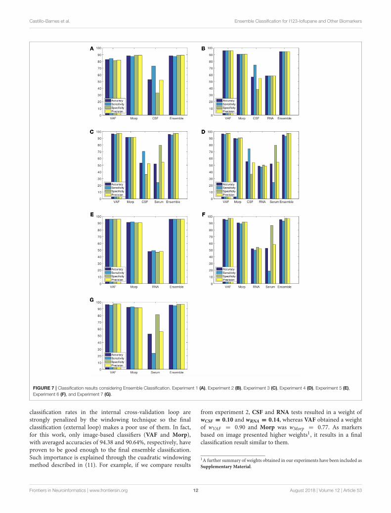
performed as shown in Table 7. Final results including individualclassifications and the ensemble fusion method are presented inFigure 7.

Although all classifications were performed using linear SVMclassifiers, as mentioned in the 1, a second battery of simulationswas also performed making use of K-Nearest Neighbor (KNN)classifiers. Results of these simulations have been included asSupplementary Material. Due to the worse classification ratesobtained with this kind of classifiers, their use was discarded.

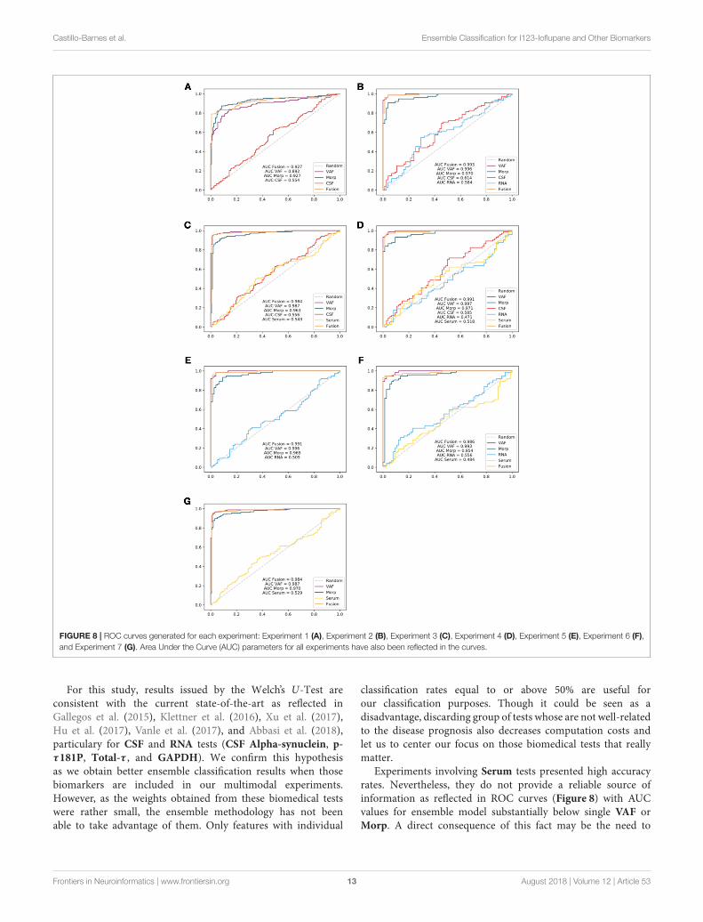
Finally, to highlight the difference between sets of medicaltests (CSF, RNA, and Serum), image features and the ensemblemodel that combines all of them; a further comparison wasperformed by means of the Receiver Operating Characteristic(ROC) curves (Zweig and Campbell, 1993) for the sevenexperiments (see Figure 8).

4. DISCUSSION AND CONCLUSIONS

Despite the interest, many questions remain open surroundingthe topic of Parkinson’s Disease. As a general view (Meireles andMassano, 2012), it is expected that combination of different data

sources will give us the necessary keys to determine preciselywhich are the origins and predictive factors of PD.

Although medical science has begun to considerneuroimaging analysis as the reference test in the diagnosisof Parkinson’s Disease (Salvatore et al., 2014), results like VAFanalysis with an accuracy up to 95% in many studies are hardlyable to be improved even by employing advanced techniquesof Machine Learning. In these terms, this work presents manysignificative strenghts: a robust classification methodology thatcombines an effective intensity normalization technique basedon the use of α-Stable distributions; a classification schemawhich maximizes models obtained for each group of markers; amultimodal CAD system that combines multiple heterogeneousdata sources and an ensemble classifier that selects the mostreliable characteristics from input sources as indicated inTables 5, 7.

If we compare our final proposal (Performance Weighting

with Cuadratic Windowing) with the baseline method (MajorityVoting) as shown inTable 7, we obtain an averaged improvement

of 7.46%. This fact reinforces our main idea: if we use better

(more discriminative) biomarkers, ensemble classification rateswill increase. As it can be checked, biomedical tests with poor

Frontiers in Neuroinformatics | www.frontiersin.org 11 August 2018 | Volume 12 | Article 53

Castillo-Barnes et al. Ensemble Classification for I123-Ioflupane and Other Biomarkers

FIGURE 7 | Classification results considering Ensemble Classification. Experiment 1 (A), Experiment 2 (B), Experiment 3 (C), Experiment 4 (D), Experiment 5 (E),

Experiment 6 (F), and Experiment 7 (G).

classification rates in the internal cross-validation loop arestrongly penalized by the windowing technique so the finalclassification (external loop) makes a poor use of them. In fact,for this work, only image-based classifiers (VAF and Morp),with averaged accuracies of 94.38 and 90.64%, respectively, haveproven to be good enough to the final ensemble classification.Such importance is explained through the cuadratic windowingmethod described in (11). For example, if we compare results

from experiment 2, CSF and RNA tests resulted in a weight ofwCSF = 0.10 and wRNA = 0.14, whereas VAF obtained a weightof wVAF = 0.90 and Morp was wMorp = 0.77. As markersbased on image presented higher weights1, it results in a finalclassification result similar to them.

1A further summary of weights obtained in our experiments have been included as

Supplementary Material.

Frontiers in Neuroinformatics | www.frontiersin.org 12 August 2018 | Volume 12 | Article 53

Castillo-Barnes et al. Ensemble Classification for I123-Ioflupane and Other Biomarkers

FIGURE 8 | ROC curves generated for each experiment: Experiment 1 (A), Experiment 2 (B), Experiment 3 (C), Experiment 4 (D), Experiment 5 (E), Experiment 6 (F),

and Experiment 7 (G). Area Under the Curve (AUC) parameters for all experiments have also been reflected in the curves.

For this study, results issued by the Welch’s U-Test areconsistent with the current state-of-the-art as reflected inGallegos et al. (2015), Klettner et al. (2016), Xu et al. (2017),Hu et al. (2017), Vanle et al. (2017), and Abbasi et al. (2018),particulary for CSF and RNA tests (CSF Alpha-synuclein, p-τ181P, Total-τ , and GAPDH). We confirm this hypothesisas we obtain better ensemble classification results when thosebiomarkers are included in our multimodal experiments.However, as the weights obtained from these biomedical testswere rather small, the ensemble methodology has not beenable to take advantage of them. Only features with individual

classification rates equal to or above 50% are useful forour classification purposes. Though it could be seen as adisadvantage, discarding group of tests whose are not well-relatedto the disease prognosis also decreases computation costs andlet us to center our focus on those biomedical tests that reallymatter.

Experiments involving Serum tests presented high accuracyrates. Nevertheless, they do not provide a reliable source ofinformation as reflected in ROC curves (Figure 8) with AUCvalues for ensemble model substantially below single VAF orMorp. A direct consequence of this fact may be the need to

Frontiers in Neuroinformatics | www.frontiersin.org 13 August 2018 | Volume 12 | Article 53

Castillo-Barnes et al. Ensemble Classification for I123-Ioflupane and Other Biomarkers

discard this type of tests defined by the PPMI in a previous phasefor future works.

In view of the obtained results, and as we can see in Figure 6

in relation to biomedical tests, no general conclusions can bedrawn for experiments that have presented p-values above 5%significance level (none of the experiments presented a p-valueunder 0.05 and only experiment 2, and experiment 4 with p-values between 0.05 and 0.1). In comparison with Welch’s U-Test in Table 3, RNA and CSF features with p-values below0.05 should be enough to discern between PD and HC subjects.However, this idea is not reflected in the permutation tests.The main reason could be the small sample size of groups:if distribution variance of accuracies increases, p-value is alsoincreased.

This CAD system can be used to determine an early diagnosisor evolution of Parkinson’s Disease. Subjects information forthe last 5, 10, 15, or 20 years may be used to determine howdisease has progressed. In this sense, if we could work usinglongitudinal information, we will face up to Parkinson’s Diseasefrom a different perspective: not only confirming if a subjectshows signs of suffering the neurological disorder but also if thatperson may develop this pathology in the future.

Though there are not many works related to the useof ensemble classification methodologies for the study ofneurodegenerative diseases, the use of Neural Networks or Tree-Based Models with different kind of classifiers as ensembleapproaches are quite prominent. Works like presented inKhan et al. (2016) and Li and Wang (2017) which made useof datasets based on speech recordings were able to reachaccuracies up to 90%. Other works like (Challa et al., 2016)also combine different imaging biomarkers with biomedicaltests to make a model of the disease. In this sense, wecould also cite the work presented in Latourelle et al. (2017)which performs a longitudinal study of Parkinsonism based onthe use of different clinical, molecular and genetic data. Thesmall size of the dataset used in some of these studies andthe computation costs in several cases may be some of thestrongest disadvantages with respect to our proposal. Only theproposal presented in Ramírez et al. (2018), for Alzheimer’sDisease diagnosis, makes use of a multi-level robust ensembleclassification model.

One last point to close this section 4 has a close relation tothe most important problem we have had to face up: the lack ofall medical tests results for all patients. Although our study wasdesigned to work with the entire PPMI database, due to the lack

of all medical tests our experiments have not been able to count

on all subjects. In this sense, threemain ideas have been suggestedfor future works:

• The inclusion of Missing Data (MD) techniques which arealready being implemented in fields like wireless networks ordata mining (Magán-Carrión et al., 2015).

• Add new promising biomarkers as referred on Saikiet al. (2017) and Delgado-Alvarado et al. (2017) or studyrelations between existing ones (Constantinides et al., 2017;Fereshtehnejad et al., 2017).

• Include new image markers as stated in Saeed et al. (2017)or make use of different image sources combined as done bySegovia et al. (2017b).

• The design of a dynamic feature selection procedure for theinternal loop which may be also used by the external ensembleloop.

In regarding to its easy adaptation, the proposed methodologypresented in this work can also be used for many otherdatabases such as ADNI (http://adni.loni.usc.edu/) or DIAN(https://dian.wustl.edu/). Moreover, the extension of thisproposal with the inclusion of procedures for semi-supervisedlearning or the use of data imputation techniques will face upwith the lack of complete tests.

AUTHOR CONTRIBUTIONS

DC-B, JR, and DS-G: conception or design of the work. DC-B, FS, and FM-M: data collection. DC-B, JR, and DS-G: dataanalysis and interpretation. DC-B, JR, JG, and DS-G: drafting ofthe article. JR, FS, FM-M, DS-G, and JG: critical revision of thearticle. DC-B, JR, DS-G, and JG: major revision of the article.

FUNDING

This work was supported by the MINECO/FEDER underthe TEC2015-64718-R project and the Ministry of Economy,Innovation, Science and Employment of the Junta de Andalucíaunder the Excellence Project P11-TIC-7103.

SUPPLEMENTARY MATERIAL

The Supplementary Material for this article can be foundonline at: https://www.frontiersin.org/articles/10.3389/fninf.2018.00053/full#supplementary-material

REFERENCES

Abbasi, N., Mohajer, B., Abbasi, S., Hasanabadi, P., Abdolalizadeh, A., and

Rajimehr, R. (2018). Relationship between cerebrospinal fluid biomarkers and

structural brain network properties in Parkinson’s disease. Mov. Disord. 33,

431–439. doi: 10.1002/mds.27284

Andersen, A. D., Binzer, M., Stenager, E., and Gramsbergen, J. B.

(2017). Cerebrospinal fluid biomarkers for Parkinson’s disease–A

systematic review. Acta Neurol. Scand. 135, 34–56. doi: 10.1111/ane.

12590

Augimeri, A., Cherubini, A., Cascini, G. L., Galea, D., Caligiuri, M. E., Barbagallo,

G., et al. (2016). CADA–computer-aided daTSCAN analysis. EJNMMI Phys.

3:4. doi: 10.1186/s40658-016-0140-9

Badoud, S., Ville, D. V. D., Nicastro, N., Garibotto, V., Burkhard, P. R.,

and Haller, S. (2016). Discriminating among degenerative Parkinsonisms

using advanced 123i-ioflupane spect analyses. Neuroimage Clin. 12(Suppl. C),

234–240. doi: 10.1016/j.nicl.2016.07.004

Blanzieri, E. and Melgani, F. (2008). Nearest neighbor classification of remote

sensing images with the maximal margin principle. IEEE Trans. Geosci. Remote

Sens. 46, 1804–1811. doi: 10.1109/TGRS.2008.916090

Frontiers in Neuroinformatics | www.frontiersin.org 14 August 2018 | Volume 12 | Article 53

Castillo-Barnes et al. Ensemble Classification for I123-Ioflupane and Other Biomarkers

Brahim, A., Górriz, J. M., Ramírez, J., and Khedher, L. (2015).

Intensity normalization of datscan spect imaging using a model-

based clustering approach. Appl. Soft Comput. 37(Suppl. C), 234–244.

doi: 10.1016/j.asoc.2015.08.030

Breiman, L., Friedman, J. H., Olshen, R. A., and Stone, C. J. (1984). Classification

and Regression Trees. Wadsworth, OH: Belmont.

Castillo-Barnes, D., Arenas, C., Segovia, F., Martinez-Murcia, F. J., Illan, I. A.,

Górriz, J. M., et al. (2017). “On a heavy-tailed intensity normalization

of the Parkinson’s progression markers initiative brain database,” in

Natural and Artificial Computation for Biomedicine and Neuroscience:

International Work-Conference on the Interplay Between Natural and

Artificial Computation, IWINAC 2017, Proceedings, Part I (Corunna: Springer

International Publishing), 298–304.

Challa, K. N. R., Pagolu, V. S., Panda, G., and Majhi, B. (2016). “An

improved approach for prediction of Parkinson’s disease using machine

learning techniques,” in 2016 International Conference on Signal Processing,

Communication, Power and Embedded System (SCOPES) (Paralakhemundi),

1446–1451.

Constantinides, V. C., Paraskevas, G. P., Emmanouilidou, E., Petropoulou,

O., Bougea, A., Vekrellis, K., et al. (2017). CSF biomarkers beta-amyloid,

tau proteins and a-synuclein in the differential diagnosis of Parkinson-plus

syndromes. J. Neurol. Sci. 382(Suppl. C), 91–95. doi: 10.1016/j.jns.2017.09.039

Dai, Z., Yan, C., Wang, Z., Wang, J., Xia, M., Li, K., et al. (2012). Discriminative

analysis of early Alzheimer’s disease using multi-modal imaging and multi-

level characterization with multi-classifier (m3). Neuroimage 59, 2187–2195.

doi: 10.1016/j.neuroimage.2011.10.003

Delgado-Alvarado, M., Gago, B., Gorostidi, A., Jiménez-Urbieta, H., Dacosta-

Aguayo, R., Navalpotro-Gómez, I., et al. (2017). Tau/alpha-synuclein ratio

and inflammatory proteins in Parkinson’s disease: an exploratory study. Mov.

Disord. 32, 1066–1073. doi: 10.1002/mds.27001

Dukart, J., Sambataro, F., and Bertolino, A. (2017). Distinct role of striatal

functional connectivity and dopaminergic loss in Parkinson’s symptoms. Front.

Aging Neurosci. 9:151. doi: 10.3389/fnagi.2017.00151

Efron, B. (1983). Estimating the error rate of a prediction rule: improvement on

cross-validation. J. Am. Stat. Assoc. 78, 316–331.

Ernst, M. D. (2004). Permutation methods: a basis for exact inference. Stat. Sci. 19,

676–685. doi: 10.1214/088342304000000396

Farotti, L., Paciotti, S., Tasegian, A., Eusebi, P., and Parnetti, L. (2017).

Discovery, validation and optimization of cerebrospinal fluid biomarkers

for use in Parkinson’s disease. Expert Rev. Mol. Diagnost. 17, 771–780.

doi: 10.1080/14737159.2017.1341312

Fauci, A. S., Braunwald, E., Kasper, D. L., Hauser, S. L., Longo, D. L., Jameson, J. L.,

et al. (2008). Harrison’s Principles of Internal Medicine (Spanish Edition), 17th

Edn., Vol. 2. McGraw-Hill.

Fereshtehnejad, S.-M., Zeighami, Y., Dagher, A., and Postuma, R. B. (2017).

Clinical criteria for subtyping Parkinson’s disease: biomarkers and longitudinal

progression. Brain 140, 1959–1976. doi: 10.1093/brain/awx118

Gallegos, S., Pacheco, C., Peters, C., Opazo, C. M., and Aguayo, L. G.

(2015). Features of alpha-synuclein that could explain the progression

and irreversibility of Parkinson’s disease. Front. Neurosci. 9:59.

doi: 10.3389/fnins.2015.00059

Garg, A., Appel-Cresswell, S., Popuri, K., McKeown, M. J., and Beg, M. F. (2015).

Morphological alterations in the caudate, putamen, pallidum, and thalamus in

Parkinson’s disease. Front. Neurosci. 9:101. doi: 10.3389/fnins.2015.00101

Good, P. I. (2006). Resampling Methods, A Practical Guide to Data Analysis, 3rd

Edn. Boston, MA: Birkhäuser.

Górriz, J. M., Ramírez, J., Suckling, J., Illan, I. A., Ortiz, A., Martinez-Murcia, F. J.,

et al. (2017a). Case-based statistical learning: a non-parametric implementation

with a conditional-error rate SVM. IEEE Access 5, 11468–11478. doi: 10.1109/

ACCESS.2017.2714579

Górriz, J. M., Ramírez, J., Suckling, J., Martinez-Murcia, F., Illan, I. A.,

Segovia, F., et al. (2017b). A semi-supervised learning approach for model

selection based on class-hypothesis testing. Expert Syst. Appl. 90, 40 – 49.

doi: 10.1016/j.eswa.2017.08.006

Handels, R. L., Vos, S. J., Kramberger, M. G., Jelic, V., Blennow, K., van Buchem,

M., et al. (2017). Predicting progression to dementia in persons with mild

cognitive impairment using cerebrospinal fluid markers. Alzheimers Dement.

13, 903–912. doi: 10.1016/j.jalz.2016.12.015

Hastie, T., Tibshirani, R., and Friedman, J. (2001). The Elements of Statistical

Learning. New York, NY: Springer.

Hu, X., Yang, Y., and Gong, D. (2017). Changes of cerebrospinal fluid aβ42, t-tau,

and p-tau in Parkinson’s disease patients with cognitive impairment relative

to those with normal cognition: a meta-analysis. Neurol. Sci. 38, 1953–1961.

doi: 10.1007/s10072-017-3088-1

Illan, I. A., Górriz, J. M., Ramírez, J., Segovia, F., Jiménez-Hoyuela, J. M.,

and Ortega Lozano, S. J. (2012). Automatic assistance to Parkinson’s

disease diagnosis in datscan spect imaging. Med. Phys. 39, 5971–5980.

doi: 10.1118/1.4742055

Khan, M. M., Chalup, S. K., and Mendes, A. (2016). “Parkinson’s disease data

classification using evolvable wavelet neural networks,” in Artificial Life and

Computational Intelligence, ACALCI 2016, eds T. Ray, R. Sarker, and X. Li

(Melbourne, VIC: Springer International Publishing), 113–124.

Klettner, A., Tholey, A., Wiegandt, A., Richert, E., Nölle, B., Deuschl, G., et al.

(2016). Reduction of gapdh in lenses of Parkinson’s disease patients: a possible

new biomarker.Mov. Disord. 32, 459–462. doi: 10.1002/mds.26863

Kohavi, R. (1995). “A study of cross-validation and bootstrap for accuracy

estimation and model selection,” in IJCAI’95 Proceedings of the 14th

International Joint Conference on Artificial Intelligence, IJCAI’95 (Québec),

1137–1145.

Kordower, J. H., Olanow, C. W., Dodiya, H. B., Chu, Y., Beach, T. G., Adler, C. H.,

et al. (2013). Disease duration and the integrity of the nigrostriatal system in

Parkinson’s disease. Brain 136, 2419–2431. doi: 10.1093/brain/awt192

Latourelle, J. C., Beste, M. T., Hadzi, T. C., Miller, R. E., Oppenheim, J. N.,

Valko, M. P., et al. (2017). Large-scale identification of clinical and genetic

predictors of motor progression in patients with newly diagnosed Parkinson’s

disease: a longitudinal cohort study and validation. Lancet Neurol. 16, 908–916.

doi: 10.1016/S1474-4422(17)30328-9

Lehman, E. L., and Romano, J. P. (2005). Testing Statistical Hypotheses, 3rd Edn.

New York, NY: Springer-Verlag.

Li, Q., Wu, X., Xu, L., Chen, K., Yao, L., and Alzheimer’s Disease Neuroimaging

Initiative. (2018). Classification of Alzheimer’s disease, mild cognitive

impairment, and cognitively unimpaired individuals using multi-feature

kernel discriminant dictionary learning. Front. Comput. Neurosci. 11:117.

doi: 10.3389/fncom.2017.00117

Li, Y., and Wang, P. (2017). Classification of Parkinson’s disease by decision tree

based instance selection and ensemble learning algorithms. J. Med. Imaging

Health Inform. 7, 444–452. doi: 10.1166/jmihi.2017.2033

Magán-Carrión, R., Camacho, J., and García-Teodoro, P. (2015). Multivariate

statistical approach for anomaly detection and lost data recovery in wireless

sensor networks. Int. J. Distrib. Sensor Netw. 11:672124. doi: 10.1155/2015/

672124

Marek, K. L., Innis, R. B., Van Dyck, C. H., Fussell, B., Early, M. Y., Eberly, S. W.,

et al. (2001). [123i] b-cit spect imaging assessment of the rate of Parkinson’s

disease progression. Neurology 57, 2089–2094. doi: 10.1212/WNL.57.11.2089

Martinez-Murcia, F., Górriz, J., Ramírez, J., Illan, I. A., and Ortiz, A. (2014).

Automatic detection of Parkinsonism using significance measures and

component analysis in datscan imaging.Neurocomputing 126(Suppl. C), 58–70.

doi: 10.1016/j.neucom.2013.01.054

Meireles, J., and Massano, J. (2012). Cognitive impairment and dementia in

Parkinson’s disease: Clinical features, diagnosis, and management. Front.

Neurol. 3:88. doi: 10.3389/fneur.2012.00088

Mollenhauer, B., Caspell-Garcia, C. J., Coffey, C. S., Taylor, P., Shaw, L. M.,

Trojanowski, J. Q., et al. (2017). Longitudinal csf biomarkers in patients

with early Parkinson disease and healthy controls. Neurology 89, 1959–1969.

doi: 10.1212/WNL.0000000000004609

Neumeyer, J. L., Wang, S., Milius, R. A., Baldwin, R. M., Zea-Ponce, Y., Hoffer,

P. B., et al. (1991). [123i]-2.beta.-carbomethoxy-3.beta.-(4-iodophenyl)tropane:

high-affinity spect (single photon emission computed tomography) radiotracer

of monoamine reuptake sites in brain. J. Med. Chem. 34, 3144–3146.

doi: 10.1021/jm00114a027

Opitz, D. W., and Shavlik, J. W. (1996). Actively searching for an effective neural

network ensemble. Connect. Sci. 8, 337–354. doi: 10.1080/095400996116802

Pohl, A., Anders, S., Chen, H., Patel, H. J., Heller, J., Reetz, K., et al. (2017).

Impaired emotional mirroring in Parkinson’s disease–A study on brain

activation during processing of facial expressions. Front. Neurol. 8:682.

doi: 10.3389/fneur.2017.00682

Frontiers in Neuroinformatics | www.frontiersin.org 15 August 2018 | Volume 12 | Article 53

Castillo-Barnes et al. Ensemble Classification for I123-Ioflupane and Other Biomarkers

Ramírez, J., Górriz, J., Ortiz, A., Martinez-Murcia, F., Segovia, F., Salas-

Gonzalez, D., et al. (2018). Ensemble of random forests one vs. rest

classifiers for MCI and AD prediction using ANOVA cortical and subcortical

feature selection and partial least squares. J. Neurosci. Methods 302, 47–57.

doi: 10.1016/j.jneumeth.2017.12.005

Ramírez, J., Górriz, J. M., Chaves, R., Lopez, M., Salas-Gonzalez, D., Alvarez, I.,

et al. (2009). Spect image classification using random forests. Electron. Lett. 45,

604–605. doi: 10.1049/el.2009.1111

Rokach, L. (2010). Pattern Classification Using Ensemble Methods, Vol 75.

Singapore: World Scientific Publishing Co. Pte. Ltd.

Saeed, U., Compagnone, J., Aviv, R. I., Strafella, A. P., Black, S. E., Lang,

A. E., et al. (2017). Imaging biomarkers in Parkinson’s disease and

Parkinsonian syndromes: current and emerging concepts. Trans. Neurodegen.

6:8. doi: 10.1186/s40035-017-0076-6

Saiki, S., Hatano, T., Fujimaki, M., Ishikawa, K.-I., Mori, A., Oji, Y., et al.

(2017). Decreased long-chain acylcarnitines from insufficient beta-oxidation

as potential early diagnostic markers for Parkinson’s disease. Sci. Rep. 7:7328.

doi: 10.1038/s41598-017-06767-y

Salas-Gonzalez, D., Górriz, J. M., Ramírez, J., Illan, I. A., and Lang, E. W.

(2013). Linear intensity normalization of FP-CIT spect brain images

using the alpha-stable distribution. Neuroimage 65(Suppl. C), 449–455.

doi: 10.1016/j.neuroimage.2012.10.005

Salas-Gonzalez, D., Kuruoglu, E. E., and Ruiz, D. P. (2009). Finite mixture

of alpha-stable distributions. Digital Signal Process. 19, 250–264.

doi: 10.1016/j.dsp.2007.11.004

Salvatore, C., Cerasa, A., Castiglioni, I., Gallivanone, F., Augimeri, A., Lopez, M.,

et al. (2014). Machine learning on brain MRI data for differential diagnosis of

Parkinson’s disease and progressive supranuclear palsy. J. Neurosci. Methods

222, 230–237. doi: 10.1016/j.jneumeth.2013.11.016

Santiago, J. A., and Potashkin, J. A. (2017). Evaluation of RNA blood biomarkers

in individuals at risk of Parkinson’s disease. J. Parkinsons Dis. 7, 653–660.

doi: 10.3233/JPD-171155

Segovia, F., Bastin, C., Salmon, E., Górriz, J. M., Ramírez, J., and Phillips,

C. (2014). Combining pet images and neuropsychological test data

for automatic diagnosis of Alzheimer’s disease. PLoS ONE 9:e88687.

doi: 10.1371/journal.pone.0088687

Segovia, F., Górriz, J., Ramírez, J., Salas-Gonzalez, D., Illan, I. A., Lopez, M., et al.

(2010). Classification of functional brain images using a GMM-based multi-

variate approach. Neurosci. Lett. 474, 58–62. doi: 10.1016/j.neulet.2010.03.010

Segovia, F., Górriz, J. M., Ramírez, J., Illan, I. A., Jimenez-Hoyuela, J. M., and

Ortega, S. J. (2012). Improved Parkinsonism diagnosis using a partial least

squares based approach.Med. Phys. 39, 4395–4403. doi: 10.1118/1.4730289

Segovia, F., Górriz, J. M., Ramírez, J., Martinez-Murcia, F. J., Castillo-Barnes, D.,

Illan, I. A., et al. (2017a). “Automatic separation of Parkinsonian patients and

control subjects based on the striatal morphology,” in Natural and Artificial

Computation for Biomedicine and Neuroscience: InternationalWork-Conference

on the Interplay Between Natural and Artificial Computation, IWINAC 2017,

Proceedings, Part I (Corunna: Springer International Publishing), 345–352.

Segovia, F., Górriz, J. M., Ramírez, J., Martinez-Murcia, F. J., Levin, J.,

Schuberth, M., et al. (2017b). Multivariate analysis of 18F-DMFP pet

data to assist the diagnosis of Parkinsonism. Front. Neuroinform. 11:23.

doi: 10.3389/fninf.2017.00023

Sixel-Döring, F., Liepe, K., Mollenhauer, B., Trautmann, E., and Trenkwalder, C.

(2011). The role of 123I-FP-CIT-spect in the differential diagnosis of Parkinson

and tremor syndromes: a critical assessment of 125 cases. J. Neurol. 258,

2147–2154. doi: 10.1007/s00415-011-6076-z

Tong, T., Gray, K., Gao, Q., Chen, L., and Rueckert, D. (2017). Multi-modal

classification of Alzheimer’s disease using nonlinear graph fusion. Patt. Recogn.

63, 171–181. doi: 10.1016/j.patcog.2016.10.009

Tzourio-Mazoyer, N., Landeau, B., Papathanassiou, D., Crivello, F., Etard, O.,

Delcroix, N., et al. (2002). Automated anatomical labeling of activations

in SPM using a macroscopic anatomical parcellation of the MNI MRI

single-subject brain. Neuroimage 15, 273–289. doi: 10.1006/nimg.2001.

0978

Vanle, B. C., Florang, V. R., Murry, D. J., Aguirre, A. L., and Doorn, J. A.

(2017). Inactivation of glyceraldehyde-3-phosphate dehydrogenase by the

dopamine metabolite, 3,4-dihydroxyphenylacetaldehyde. Biochem. Biophys.

Res. Commun. 492, 275–281. doi: 10.1016/j.bbrc.2017.08.067

Vapnik, V. N. (1998). Statistical Learning Theory, Edn. 1. New York, NY: John

Wiley & Sons.

Wyman-Chick, K., Martin, P., Minár, M., and Schroeder, R. (2016). Cognition

in patients with a clinical diagnosis of Parkinson disease and scans without

evidence of dopaminergic deficit (SWEDD): 2-year follow-up. Cogn. Behav.

Neurol. 29, 190–196. doi: 10.1097/WNN.0000000000000107

Xu, C.-Y., Kang, W.-Y., Chen, Y.-M., Jiang, T.-F., Zhang, J., Zhang,

L.-N., et al. (2017). DJ-1 inhibits alpha-synuclein aggregation by

regulating chaperone-mediated autophagy. Front. Aging Neurosci. 9:308.

doi: 10.3389/fnagi.2017.00308

Zetterström, R. H., Solomin, L., Jansson, L., Hoffer, B. J., Olson, L., and Perlmann,

T. (1997). Dopamine neuron agenesis in Nurr1-deficient mice. Science 276,

248–250. doi: 10.1126/science.276.5310.248

Zweig, M. H., and Campbell, G. (1993). Receiver-operating characteristic (ROC)

plots: a fundamental evaluation tool in clinical medicine. Clin. Chem. 39,

561–577.

Conflict of Interest Statement: The authors declare that the research was

conducted in the absence of any commercial or financial relationships that could

be construed as a potential conflict of interest.

Copyright © 2018 Castillo-Barnes, Ramírez, Segovia, Martínez-Murcia, Salas-

Gonzalez and Górriz. This is an open-access article distributed under the terms

of the Creative Commons Attribution License (CC BY). The use, distribution or

reproduction in other forums is permitted, provided the original author(s) and the

copyright owner(s) are credited and that the original publication in this journal

is cited, in accordance with accepted academic practice. No use, distribution or

reproduction is permitted which does not comply with these terms.

Frontiers in Neuroinformatics | www.frontiersin.org 16 August 2018 | Volume 12 | Article 53