Embed Size (px)
Citation preview
1
Robust estimation of historical volatility and correlations in risk management
Alexander Tchernitser and Dmitri H. Rubisov1
This version: March 19, 20052
Abstract Financial time series have two features which, in many cases, prevent the use of conventional estimators of volatilities and correlations: leptokurtotic tails of data distributions, and contamination of data with outliers. Robust estimators are required to achieve stable and accurate results. In this paper, we review robust estimators for volatilities and correlations and identify those best suited for use in risk management. The selection criteria were that the estimator should be stable to both fractionally small departures for all data points (fat tails), or fractionally large departures for a small number of data points (outliers). Since risk management typically deals with thousands of time series at once, another major requirement was the independence of the approach of any manual correction or data pre-processing. We recommend using volatility t-estimators, for which we derived the estimation error formula for the case when the exact shape of the data distribution is unknown. The most convenient robust estimator for correlations is Kendall’s tau, whose major drawback is that it does not guarantee the positivity of the correlation matrix. We propose an algorithm that overcomes this problem by finding the closest correlation matrix to a given matrix.
Keywords Robust estimation, historical volatility, correlation, outliers, estimation accuracy, positive definite.
1 Market Risk, Enterprise Risk and Portfolio Management, BMO Financial Group, 100 King Street West, 3rd floor FCP,
Toronto, Ontario, M5X 1A1. [email protected] or [email protected]. This article expresses
the views of the authors and not necessarily the view of the Bank of Montreal. 2 First version was presented at the Department of Statistics, University of Toronto, on January 29, 2004.
2
1 Introduction Most financial models used to quantify dependent risks are based on the assumption of multivariate normality, and sample standard deviation and linear correlation are used as measures of volatility and dependence. However, observed financial data distributions are rarely normal. Quite opposite, they tend to have leptokurtotic marginal distributions with heavier tails. It is also typical to see them contaminated with outliers. Consequently, the standard estimators, such as sample variance/volatility and Pearson’s product-moment correlation coefficient, which are optimal for uncontaminated multivariate normal distributions, have very little chance to correctly estimate statistical parameters due to unconstrained dependency on the behaviour of tails. In order to achieve stable estimates of volatilities and correlations, a different type of the estimation technique is deemed necessary. This technique is usually termed parametric robust estimation. The term “robust estimator” does not have a unified definition. In general, the term refers to a statistical parameter estimator that is insensitive to small departures from the idealized assumptions for which the estimator was optimized (Huber, 1981, Press et al., 1992). This definition requires further elaboration though, as the term “small departures” may be interpreted in two different ways. Small departures can either be fractionally small departures for all data points, or fractionally large departures for a small number of data points. Both interpretations are relevant in finance and consequently an ideal estimator should be stable to both. The former is associated with the distribution non-normality such as heavier tails and sharper peak, whereas the latter leads to the notion of outliers. It is the presence of outliers that is very often responsible for significant miscalculation of statistical parameters. In this paper we review robust estimators for volatilities and correlations and identify those best suited for the use in risk management. Risk management typically deals with thousands of time series, and one of our major requirements was that the technique can “run unattended”. For volatilities, we recommend using t-estimators, described in Section 2, where we also derive a formula for the estimation error for the case when the exact shape of the data distribution is unknown. A very stable and convenient robust estimator for correlations is Kendall’s tau, discussed in Section 3. In that section, we also propose an algorithm that finds the closest correlation matrix to a given matrix. This is necessary because pair-wise robust correlation estimators do not guarantee the positivity of the correlation matrix. Examples are also provided in both sections.
2 Robust Estimation of Volatilities
2.1 Review
The idea of using robust estimations in data modelling first appeared in the early fifties. One of the first robust estimators of linear regression, based on the combination of sample variance close to the centre of the distribution and sum of absolute values in the tales, was
3
introduced by Huber (1981). Although this estimator does not satisfy one of the robustness criteria of the previous section since it is still very sensitive to outliers, its historical merit cannot be overstated. The sensitivity of the estimator to unbounded outliers is usually quantified using the notion of “breaking point”, defined as the fraction of points in a sample whose unbounded errors do not send the total variance of the parameter estimate to infinity3. In terms of the breaking point, the most robust estimators are median absolute deviation (MAD) and inter-quartile distance (IQD). The first one is defined as:
MAD = Median (|xi – µ|) (2.1)
where µ is the median of the time series xi, i = 1…n. The second is the distance between the 25% and 75% quantiles of the sample. Both estimators have maximum breaking point of 50%, same as their more advanced counterparts, termed S and Q-estimators (Croux and Rousseeuw, 1992). The major problem preventing their wide use in financial applications is that all those estimators completely ignore information from the distribution tails; specifically, 50% of the sample is ignored. The consequences can be illustrated with the following example. Many financial time series have extended periods of so-called sticky prices, over which the value of the random variable does not change and hence the returns are zero all this time. For example, if a stock price changes twice a week (that may correspond to the frequency of trades of that particular stock), 60% of all daily returns on this stock are zero, and MAD and IQD would produce zero estimates of the stock volatility4. Another very robust group of scale estimators are based on a certain way of data censoring (trimming). Data trimming algorithms heavily depend on the number (or fraction) of points trimmed, which effectively becomes the major parameter of the estimator and stipulates its breaking point. It does not seem possible to select this parameter without a priori knowledge of the degree of contamination of the distribution. Since this information is usually unavailable, especially if data from different markets and different sources are analysed, it is desirable to avoid forced and predetermined trimming of data. A large group of estimation techniques, usually termed M-estimates, follow from maximum-likelihood arguments very much as regular sample variance follows from minimizing Gaussian deviates. The estimators have a general form:
( ) ( )∑ =
−−−=
n
i ixfn1
12 1 µσ (2.2)
where the data transform function f depends on the selection of the distribution function. If f(x) = x
2, formula (2.2) becomes the familiar sample variance formula. M-estimates form the most relevant class for estimation of parameters, when the type of the distribution is known
3 More often instead of the total variance, breaking point is defined in terms of the estimation efficiency, which is the
reciprocal of the total variance of the parameter estimate. 4 Sticky prices may require a special treatment before applying other types of estimators. Discussion of these treatments
is out of the scope of this paper.
4
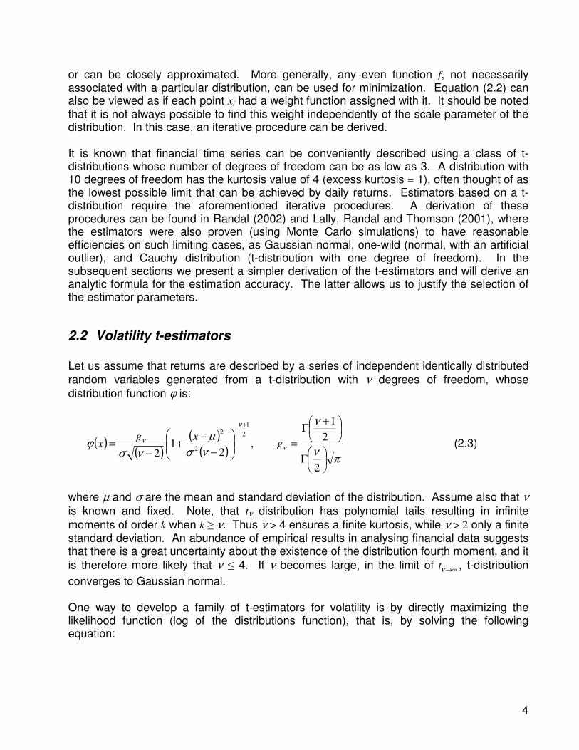
or can be closely approximated. More generally, any even function f, not necessarily associated with a particular distribution, can be used for minimization. Equation (2.2) can also be viewed as if each point xi had a weight function assigned with it. It should be noted that it is not always possible to find this weight independently of the scale parameter of the distribution. In this case, an iterative procedure can be derived. It is known that financial time series can be conveniently described using a class of t-distributions whose number of degrees of freedom can be as low as 3. A distribution with 10 degrees of freedom has the kurtosis value of 4 (excess kurtosis = 1), often thought of as the lowest possible limit that can be achieved by daily returns. Estimators based on a t-distribution require the aforementioned iterative procedures. A derivation of these procedures can be found in Randal (2002) and Lally, Randal and Thomson (2001), where the estimators were also proven (using Monte Carlo simulations) to have reasonable efficiencies on such limiting cases, as Gaussian normal, one-wild (normal, with an artificial outlier), and Cauchy distribution (t-distribution with one degree of freedom). In the subsequent sections we present a simpler derivation of the t-estimators and will derive an analytic formula for the estimation accuracy. The latter allows us to justify the selection of the estimator parameters.
2.2 Volatility t-estimators
Let us assume that returns are described by a series of independent identically distributed
random variables generated from a t-distribution with ν degrees of freedom, whose
distribution function ϕ is:
( )( )
( )( )
πν
ν
νσ
µ
νσϕ ν
ν
ν
Γ
+Γ
=
−
−+
−=
+−
2
2
1
,2
12
2
1
2
2
gxg
x (2.3)
where µ and σ are the mean and standard deviation of the distribution. Assume also that ν
is known and fixed. Note, that tν distribution has polynomial tails resulting in infinite
moments of order k when k ≥ ν. Thus ν > 4 ensures a finite kurtosis, while ν > 2 only a finite standard deviation. An abundance of empirical results in analysing financial data suggests that there is a great uncertainty about the existence of the distribution fourth moment, and it
is therefore more likely that ν ≤ 4. If ν becomes large, in the limit of ∞→νt , t-distribution
converges to Gaussian normal. One way to develop a family of t-estimators for volatility is by directly maximizing the likelihood function (log of the distributions function), that is, by solving the following equation:
5
( )( )0
,ln1 1 =∂
∂ ∏ =
σ
σϕn
i ix
n (2.4)
Substituting ϕ in (2.4) with (2.3), the following formulae can be obtained.
( )∑ −=n
t
tt Xwn
2
0
2 ˆ1
ˆ µσ (2.5)
∑
∑=
n
t
t
n
t
tt
w
Xw
µ̂ (2.6)
{ } ( )( )
1
2
0
2
00
ˆ2
ˆ1
2
1−
−
−+
−
+==
σν
µ
ν
ν ttt
XXSw E (2.7)
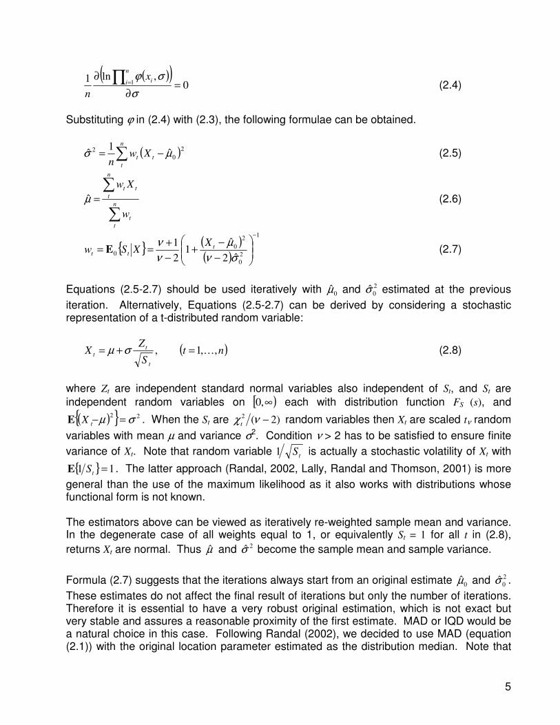
Equations (2.5-2.7) should be used iteratively with 0µ̂ and 2
0σ̂ estimated at the previous
iteration. Alternatively, Equations (2.5-2.7) can be derived by considering a stochastic representation of a t-distributed random variable:
( )ntS
ZX
t
tt ,,1, K=+= σµ (2.8)
where Zt are independent standard normal variables also independent of St, and St are
independent random variables on [ )∞,0 each with distribution function FS (s), and
( ){ } 22σµ =−tXE . When the St are )2(2 −νχι random variables then Xt are scaled tν random
variables with mean µ and variance σ2. Condition ν > 2 has to be satisfied to ensure finite
variance of Xt. Note that random variable tS1 is actually a stochastic volatility of Xt with
{ } 11 =tSE . The latter approach (Randal, 2002, Lally, Randal and Thomson, 2001) is more
general than the use of the maximum likelihood as it also works with distributions whose functional form is not known. The estimators above can be viewed as iteratively re-weighted sample mean and variance. In the degenerate case of all weights equal to 1, or equivalently St = 1 for all t in (2.8),
returns Xt are normal. Thus µ̂ and 2σ̂ become the sample mean and sample variance.
Formula (2.7) suggests that the iterations always start from an original estimate 0µ̂ and 2
0σ̂ .
These estimates do not affect the final result of iterations but only the number of iterations. Therefore it is essential to have a very robust original estimation, which is not exact but very stable and assures a reasonable proximity of the first estimate. MAD or IQD would be a natural choice in this case. Following Randal (2002), we decided to use MAD (equation (2.1)) with the original location parameter estimated as the distribution median. Note that
6
MAD involves two sortings of time series, which is an (n ln n) process. If the data series becomes excessively long (say 10 years of daily data, i.e. 2500 points), the use of MAD can be too computation extensive. In this case, it can be replaced by a less robust but faster estimator, such as the sum of absolute values or a data trimming procedure. In most financial applications, where relative or log returns are analysed, it can be safely
assumed that the distribution mean is zero, i.e. µ = 0. Then, the t-estimator for variance/volatility takes the following simplified form:
( )( )∑∑
==
=−+
−
+=
n
t
t
n
t t
t XfnX
X
n 1
2
12
0
2
22 1
ˆ212
11ˆ
σνν
νσ (2.9)
which makes the non-linear nature of the estimator more transparent.
2.3 Estimator accuracy
The only parameter of the iterative procedure (2.5-2.7) is the number of degrees of freedom
of the t-distribution, ν. Randal (2002) and Lally, Randal and Thomson (2001) used ν = 5 to construct a volatility estimator for very short time series of 20 points, to analyse moving volatilities of stocks. They did not present a detailed explanation of such selection, except that it presents an acceptable compromise between efficiencies on various distribution types. We will attempt to approach the selection of the estimator parameter from a more elaborated position. Assume our a priori knowledge of the distribution type (t-distribution) as well as of the range
for the distribution parameter ν0 (number of degrees of freedom) being from ν1 to ν2. Since
the estimator parameter ν is not necessarily the same as the parameter of the real
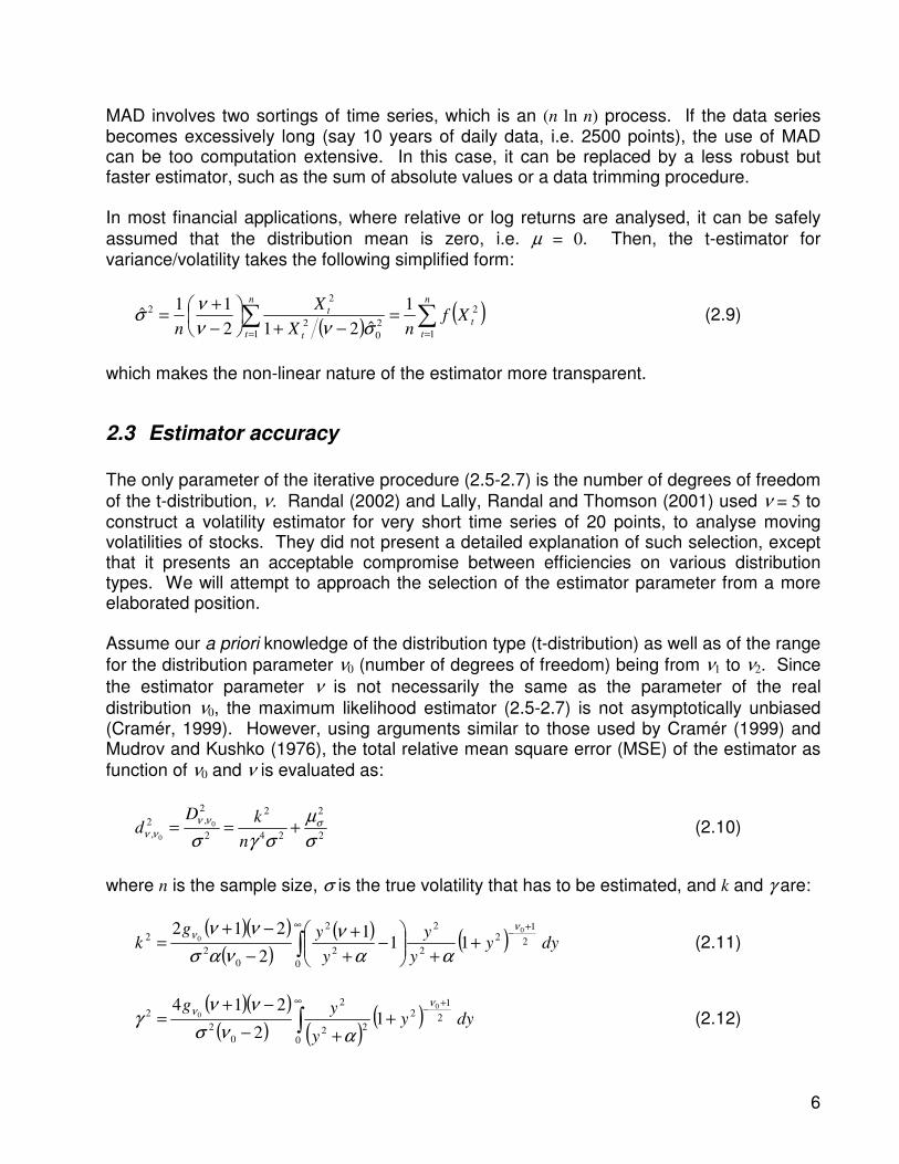
distribution ν0, the maximum likelihood estimator (2.5-2.7) is not asymptotically unbiased (Cramér, 1999). However, using arguments similar to those used by Cramér (1999) and Mudrov and Kushko (1976), the total relative mean square error (MSE) of the estimator as
function of ν0 and ν is evaluated as:
2
2
24
2
2
2
,2
,0
0 σ
µ
σγσσνν
νν +==n
kDd (2.10)
where n is the sample size, σ is the true volatility that has to be estimated, and k and γ are:
( )( )( )
( ) ( )∫∞ +
−+
+
−
+
+
−
−+=
0
2
12
2
2
2
2
0
2
20
0 111
2
212dyy
y
y
y
ygk
νν
αα
ν
νασ
νν (2.11)
( )( )( ) ( )
( )∫∞ +
−+
+−
−+=
0
2
12
22
2
0
2
20
0 12
214dyy
y
yg νν
ανσ
ννγ (2.12)
7
and finally α, defined as ( )2
21
0
2
−
−+=
ν
νσµα σ , is found from:
( ) ( ) 0111
0
2
12
2
20
=+
−
+
+∫∞ +
−dyy
y
y ν
α
ν (2.13)
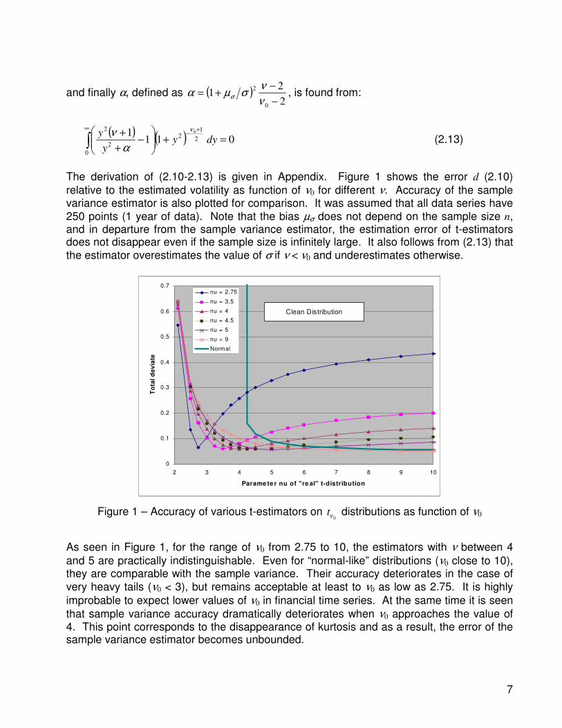
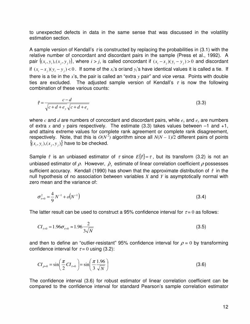
The derivation of (2.10-2.13) is given in Appendix. Figure 1 shows the error d (2.10)
relative to the estimated volatility as function of ν0 for different ν. Accuracy of the sample variance estimator is also plotted for comparison. It was assumed that all data series have
250 points (1 year of data). Note that the bias µσ does not depend on the sample size n, and in departure from the sample variance estimator, the estimation error of t-estimators does not disappear even if the sample size is infinitely large. It also follows from (2.13) that
the estimator overestimates the value of σ if ν < ν0 and underestimates otherwise.
0
0.1
0.2
0.3
0.4
0.5
0.6
0.7
2 3 4 5 6 7 8 9 10
Parame te r nu of "re al" t-distribution
To
tal
de
via
te
nu = 2.75
nu = 3.5
nu = 4
nu = 4.5
nu = 5
nu = 9
Normal
Clean Distribution
Figure 1 – Accuracy of various t-estimators on 0νt distributions as function of ν0
As seen in Figure 1, for the range of ν0 from 2.75 to 10, the estimators with ν between 4
and 5 are practically indistinguishable. Even for “normal-like” distributions (ν0 close to 10), they are comparable with the sample variance. Their accuracy deteriorates in the case of
very heavy tails (ν0 < 3), but remains acceptable at least to ν0 as low as 2.75. It is highly
improbable to expect lower values of ν0 in financial time series. At the same time it is seen
that sample variance accuracy dramatically deteriorates when ν0 approaches the value of 4. This point corresponds to the disappearance of kurtosis and as a result, the error of the sample variance estimator becomes unbounded.
8
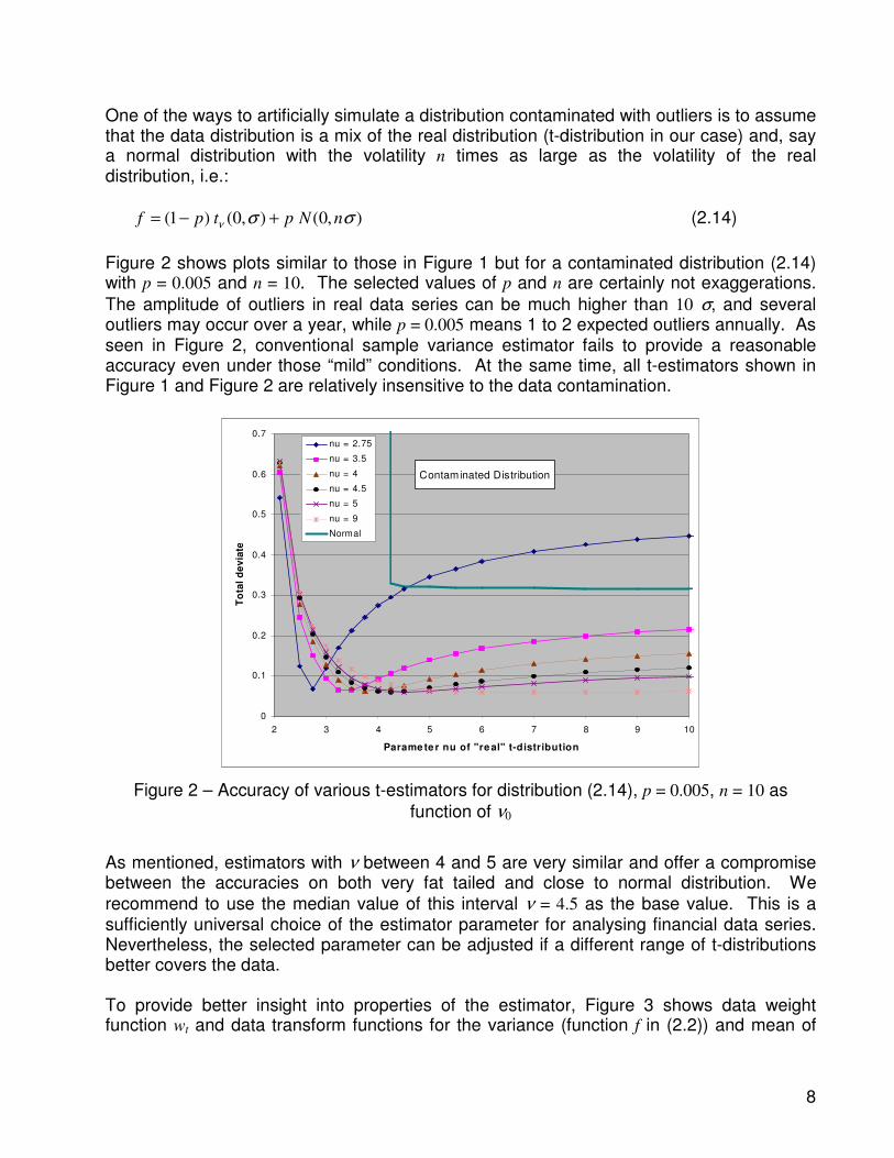
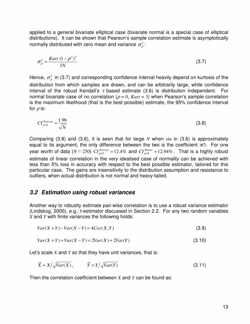
One of the ways to artificially simulate a distribution contaminated with outliers is to assume that the data distribution is a mix of the real distribution (t-distribution in our case) and, say a normal distribution with the volatility n times as large as the volatility of the real distribution, i.e.:
),0(),0()1( σσν nNptpf +−= (2.14)
Figure 2 shows plots similar to those in Figure 1 but for a contaminated distribution (2.14) with p = 0.005 and n = 10. The selected values of p and n are certainly not exaggerations.
The amplitude of outliers in real data series can be much higher than 10 σ, and several outliers may occur over a year, while p = 0.005 means 1 to 2 expected outliers annually. As seen in Figure 2, conventional sample variance estimator fails to provide a reasonable accuracy even under those “mild” conditions. At the same time, all t-estimators shown in Figure 1 and Figure 2 are relatively insensitive to the data contamination.
0
0.1
0.2
0.3
0.4
0.5
0.6
0.7
2 3 4 5 6 7 8 9 10
Parame te r nu of "re al" t-distribution
To
tal
de
via
te
nu = 2.75
nu = 3.5
nu = 4
nu = 4.5
nu = 5
nu = 9
Normal
Contaminated Distribution
Figure 2 – Accuracy of various t-estimators for distribution (2.14), p = 0.005, n = 10 as
function of ν0
As mentioned, estimators with ν between 4 and 5 are very similar and offer a compromise between the accuracies on both very fat tailed and close to normal distribution. We
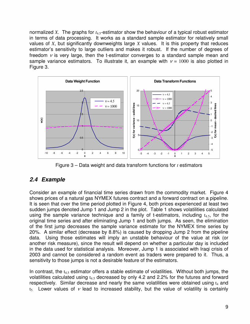
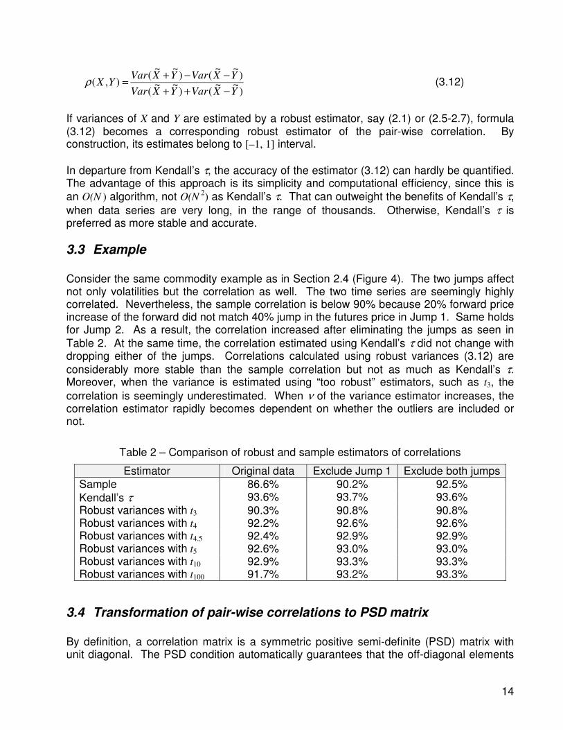
recommend to use the median value of this interval ν = 4.5 as the base value. This is a sufficiently universal choice of the estimator parameter for analysing financial data series. Nevertheless, the selected parameter can be adjusted if a different range of t-distributions better covers the data. To provide better insight into properties of the estimator, Figure 3 shows data weight function wt and data transform functions for the variance (function f in (2.2)) and mean of
9
normalized X. The graphs for t4.5-estimator show the behaviour of a typical robust estimator in terms of data processing. It works as a standard sample estimator for relatively small values of X, but significantly downweights large X values. It is this property that reduces estimator’s sensitivity to large outliers and makes it robust. If the number of degrees of
freedom ν is very large, then the t-estimator converges to a standard sample mean and
sample variance estimators. To illustrate it, an example with ν = 1000 is also plotted in Figure 3.
Data Weight Function
0
0.5
1
1.5
2
2.5
-10 -8 -6 -4 -2 0 2 4 6 8 10x
w(x
)
ν = 4.5
ν = 1000
Data Transform Functions
0
5
10
15
20
-5 -4 -3 -2 -1 0 1 2 3 4 5x
f(x
) fo
r v
ari
an
ce
- s
olid
lin
es
-5
-4
-3
-2
-1
0
1
2
3
4
5
f(x
) fo
r m
ea
n -
da
sh
ed
lin
es
ν = 4.5
ν = 1000
ν = 4.5
ν = 1000
Figure 3 – Data weight and data transform functions for t estimators
2.4 Example
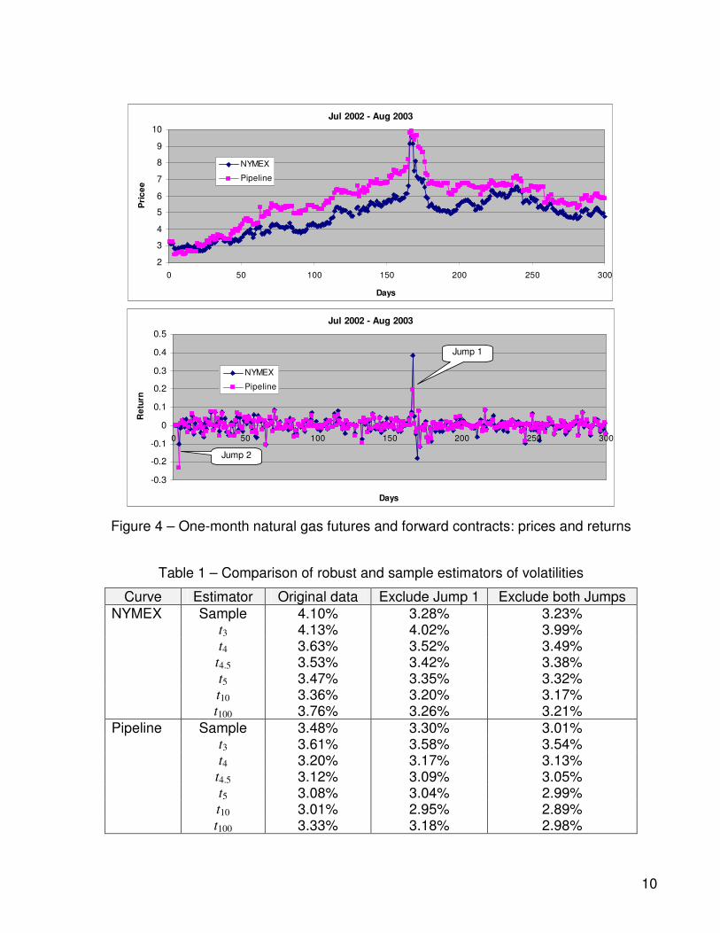
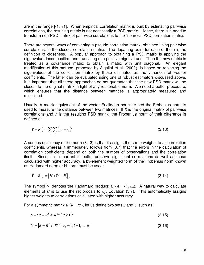
Consider an example of financial time series drawn from the commodity market. Figure 4 shows prices of a natural gas NYMEX futures contract and a forward contract on a pipeline. It is seen that over the time period plotted in Figure 4, both prices experienced at least two sudden jumps denoted Jump 1 and Jump 2 in the plot. Table 1 shows volatilities calculated using the sample variance technique and a family of t-estimators, including t4.5, for the original time series and after eliminating Jump 1 and both jumps. As seen, the elimination of the first jump decreases the sample variance estimate for the NYMEX time series by 20%. A similar effect (decrease by 8.8%) is caused by dropping Jump 2 from the pipeline data. Using those estimates will imply an unstable behaviour of the value at risk (or another risk measure), since the result will depend on whether a particular day is included in the data used for statistical analysis. Moreover, Jump 1 is associated with Iraqi crisis of 2003 and cannot be considered a random event as traders were prepared to it. Thus, a sensitivity to those jumps is not a desirable feature of the estimators. In contrast, the t4.5 estimator offers a stable estimate of volatilities. Without both jumps, the volatilities calculated using t4.5 decreased by only 4.2 and 2.2% for the futures and forward respectively. Similar decrease and nearly the same volatilities were obtained using t4 and
t5. Lower values of ν lead to increased stability, but the value of volatility is certainly
10
Jul 2002 - Aug 2003
2
3
4
5
6
7
8
9
10
0 50 100 150 200 250 300
Days
Pri
ce
e
NYMEX
Pipeline
Jul 2002 - Aug 2003
-0.3
-0.2
-0.1
0
0.1
0.2
0.3
0.4
0.5
0 50 100 150 200 250 300
Days
Re
turn
NYMEX
Pipeline
Jump 1
Jump 2
Figure 4 – One-month natural gas futures and forward contracts: prices and returns
Table 1 – Comparison of robust and sample estimators of volatilities
Curve Estimator Original data Exclude Jump 1 Exclude both Jumps NYMEX Sample 4.10% 3.28% 3.23% t3 4.13% 4.02% 3.99% t4 3.63% 3.52% 3.49% t4.5 3.53% 3.42% 3.38% t5 3.47% 3.35% 3.32% t10 3.36% 3.20% 3.17% t100 3.76% 3.26% 3.21% Pipeline Sample 3.48% 3.30% 3.01% t3 3.61% 3.58% 3.54% t4 3.20% 3.17% 3.13% t4.5 3.12% 3.09% 3.05% t5 3.08% 3.04% 2.99% t10 3.01% 2.95% 2.89% t100 3.33% 3.18% 2.98%
11
overestimated. As ν increases the estimator starts loosing the robustness property, but
even at ν = 100, it does not give the same result as the sample estimator.
3 Robust Estimation of Correlations
3.1 Estimation using Kendall’s tau
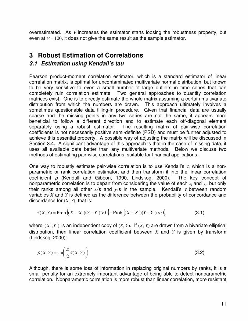
Pearson product-moment correlation estimator, which is a standard estimator of linear correlation matrix, is optimal for uncontaminated multivariate normal distribution, but known to be very sensitive to even a small number of large outliers in time series that can completely ruin correlation estimate. Two general approaches to quantify correlation matrices exist. One is to directly estimate the whole matrix assuming a certain multivariate distribution from which the numbers are drawn. This approach ultimately involves a sometimes questionable data filling-in procedure. Given that financial data are usually sparse and the missing points in any two series are not the same, it appears more beneficial to follow a different direction and to estimate each off-diagonal element separately using a robust estimator. The resulting matrix of pair-wise correlation coefficients is not necessarily positive semi-definite (PSD) and must be further adjusted to achieve this essential property. A possible way of adjusting the matrix will be discussed in Section 3.4. A significant advantage of this approach is that in the case of missing data, it uses all available data better than any multivariate methods. Below we discuss two methods of estimating pair-wise correlations, suitable for financial applications.
One way to robustly estimate pair-wise correlation is to use Kendall’s τ, which is a non-parametric or rank correlation estimator, and then transform it into the linear correlation
coefficient ρ (Kendall and Gibbon, 1990, Lindskog, 2000). The key concept of nonparametric correlation is to depart from considering the value of each xi and yi, but only
their ranks among all other xi’s and yi’s in the sample. Kendall’s τ between random variables X and Y is defined as the difference between the probability of concordance and discordance for (X, Y), that is:
{ } { }0))(( Prob0))(( Prob),( '''' <−−−>−−= YYXXYYXXYXτ (3.1)
where ),( '' YX is an independent copy of (X, Y). If (X, Y) are drawn from a bivariate elliptical
distribution, then linear correlation coefficient between X and Y is given by transform (Lindskog, 2000):
= ),(
2sin),( YXYX τ
πρ (3.2)
Although, there is some loss of information in replacing original numbers by ranks, it is a small penalty for an extremely important advantage of being able to detect nonparametric correlation. Nonparametric correlation is more robust than linear correlation, more resistant
12
to unexpected defects in data in the same sense that was discussed in the volatility estimation section.
A sample version of Kendall’s τ is constructed by replacing the probabilities in (3.1) with the relative number of concordant and discordant pairs in the sample (Press et al., 1992). A
pair ( )),(),,( jjii yxyx , where i > j, is called concordant if 0))(( >−− jiji yyxx and discordant
if 0))(( <−− jiji yyxx . If some of the xi’s or/and yi’s have identical values it is called a tie. If
there is a tie in the x’s, the pair is called an “extra y pair” and vice versa. Points with double
ties are excluded. The adjusted sample version of Kendall’s τ is now the following combination of these various counts:
xy edcedc
dc
++++
−=τ̂ (3.3)
where c and d are numbers of concordant and discordant pairs, while ex and ey are numbers of extra x and y pairs respectively. The estimate (3.3) takes values between –1 and +1, and attains extreme values for complete rank agreement or complete rank disagreement, respectively. Note, that this is O(N
2) algorithm since all N(N – 1)/2 different pairs of points
{ }),(),,( jjii yxyx have to be checked.
Sample τ̂ is an unbiased estimator of τ since { } ττ =ˆE , but its transform (3.2) is not an
unbiased estimator of ρ. However, τρ̂ estimate of linear correlation coefficient ρ possesses
sufficient accuracy. Kendall (1990) has shown that the approximate distribution of τ̂ in the null hypothesis of no association between variables X and Y is asymptotically normal with zero mean and the variance of:
( )112
09
4 −−= += NoNτσ (3.4)
The latter result can be used to construct a 95% confidence interval for τ = 0 as follows:
NCI
3
296.196.1 00 ≈= == ττ σ (3.5)
and then to define an “outlier-resistant” 95% confidence interval for ρ = 0 by transforming
confidence interval for τ = 0 using (3.2):
=
= ==
NCICI
96.1
3sin
2sin 00
ππτρ (3.6)
The confidence interval (3.6) for robust estimator of linear correlation coefficient can be compared to the confidence interval for standard Pearson’s sample correlation estimator
13
applied to a general bivariate elliptical case (bivariate normal is a special case of elliptical distributions). It can be shown that Pearson’s sample correlation estimate is asymptotically
normally distributed with zero mean and variance 2
ρσ :
N
Kurt
3
)1( 222 ρ
σ ρ
−= (3.7)
Hence, 2
ρσ in (3.7) and corresponding confidence interval heavily depend on kurtosis of the
distribution from which samples are drawn, and can be arbitrarily large, while confidence
interval of the robust Kendall’s τ based estimate (3.6) is distribution independent. For
normal bivariate case of no correlation (ρ = 0, Kurt = 3) when Pearson’s sample correlation is the maximum likelihood (that is the best possible) estimate, the 95% confidence interval
for ρ is:
NCI Pearson 96.1
0 ==ρ (3.8)
Comparing (3.8) and (3.6), it is seen that for large N when sin in (3.6) is approximately
equal to its argument, the only difference between the two is the coefficient π/3. For one
year worth of data (N ≈ 250) %4.120 ==Pearson
CI ρ and %94.120 ==Robust
CI ρ . That is a highly robust
estimate of linear correlation in the very idealised case of normality can be achieved with less than 5% loss in accuracy with respect to the best possible estimator, tailored for this particular case. The gains are insensitivity to the distribution assumption and resistance to outliers, when actual distribution is not normal and heavy-tailed.
3.2 Estimation using robust variances
Another way to robustly estimate pair-wise correlation is to use a robust variance estimator (Lindskog, 2000), e.g., t-estimator discussed in Section 2.2. For any two random variables X and Y with finite variances the following holds:
),(4)()( YXCovYXVarYXVar =−−+ (3.9)
)(2)(2)()( YVarXVarYXVarYXVar +=−++ (3.10)
Let’s scale X and Y so that they have unit variances, that is:
)(~
,)(~
YVarYYXVarXX == (3.11)
Then the correlation coefficient between X and Y can be found as:
14
)~~
()~~
(
)~~
()~~
(),(
YXVarYXVar
YXVarYXVarYX
−++
−−+=ρ (3.12)
If variances of X and Y are estimated by a robust estimator, say (2.1) or (2.5-2.7), formula (3.12) becomes a corresponding robust estimator of the pair-wise correlation. By construction, its estimates belong to [–1, 1] interval.
In departure from Kendall’s τ, the accuracy of the estimator (3.12) can hardly be quantified. The advantage of this approach is its simplicity and computational efficiency, since this is
an O(N ) algorithm, not O(N
2) as Kendall’s τ. That can outweight the benefits of Kendall’s τ,
when data series are very long, in the range of thousands. Otherwise, Kendall’s τ is preferred as more stable and accurate.
3.3 Example
Consider the same commodity example as in Section 2.4 (Figure 4). The two jumps affect not only volatilities but the correlation as well. The two time series are seemingly highly correlated. Nevertheless, the sample correlation is below 90% because 20% forward price increase of the forward did not match 40% jump in the futures price in Jump 1. Same holds for Jump 2. As a result, the correlation increased after eliminating the jumps as seen in
Table 2. At the same time, the correlation estimated using Kendall’s τ did not change with dropping either of the jumps. Correlations calculated using robust variances (3.12) are
considerably more stable than the sample correlation but not as much as Kendall’s τ. Moreover, when the variance is estimated using “too robust” estimators, such as t3, the
correlation is seemingly underestimated. When ν of the variance estimator increases, the correlation estimator rapidly becomes dependent on whether the outliers are included or not.
Table 2 – Comparison of robust and sample estimators of correlations
Estimator Original data Exclude Jump 1 Exclude both jumps
Sample 86.6% 90.2% 92.5%
Kendall’s τ 93.6% 93.7% 93.6%
Robust variances with t3 90.3% 90.8% 90.8% Robust variances with t4 92.2% 92.6% 92.6% Robust variances with t4.5 92.4% 92.9% 92.9% Robust variances with t5 92.6% 93.0% 93.0% Robust variances with t10 92.9% 93.3% 93.3% Robust variances with t100 91.7% 93.2% 93.3%
3.4 Transformation of pair-wise correlations to PSD matrix
By definition, a correlation matrix is a symmetric positive semi-definite (PSD) matrix with unit diagonal. The PSD condition automatically guarantees that the off-diagonal elements
15
are in the range [-1, +1]. When empirical correlation matrix is built by estimating pair-wise correlations, the resulting matrix is not necessarily a PSD matrix. Hence, there is a need to transform non-PSD matrix of pair-wise correlations to the “nearest” PSD correlation matrix. There are several ways of converting a pseudo-correlation matrix, obtained using pair-wise correlations, to the closest correlation matrix. The departing point for each of them is the definition of closeness. A popular approach to obtaining a PSD matrix is applying the eigenvalue decomposition and truncating non-positive eigenvalues. Then the new matrix is treated as a covariance matrix to obtain a matrix with unit diagonal. An elegant modification of this method, proposed by Alqallaf et al. (2002), is based on replacing the eigenvalues of the correlation matrix by those estimated as the variances of Fourier coefficients. The latter can be evaluated using one of robust estimators discussed above. It is important that all those approaches do not guarantee that the new PSD matrix will be closest to the original matrix in light of any reasonable norm. We need a better procedure, which ensures that the distance between matrices is appropriately measured and minimized. Usually, a matrix equivalent of the vector Euclidean norm termed the Frobenius norm is used to measure the distance between two matrices. If R is the original matrix of pair-wise correlations and Y is the resulting PSD matrix, the Frobenius norm of their difference is defined as:
( )∑∑ −=−i j
ijijFryRY
22 (3.13)
A serious deficiency of the norm (3.13) is that it assigns the same weights to all correlation coefficients, whereas it immediately follows from (3.7) that the errors in the calculation of correlation coefficients depend on both the number of observations and the correlation itself. Since it is important to better preserve significant correlations as well as those calculated with higher accuracy, a by-element weighted form of the Frobenius norm known as Hadamard norm or H-norm must be used:
( )FH
RYHRY −=− o (3.14)
The symbol “º” denotes the Hadamard product: H º A = (hij aij). A natural way to calculate
elements of H is to use the reciprocals to σρ, Equation (3.7). This automatically assigns higher weights to correlations calculated with higher accuracy. For a symmetric matrix R (R = R
T), let us define two sets S and U such as:
{ }0≥∈== RRRRS nxnTM (3.15)
{ }nirRRRU ii
nxnT ,,1,1 KM ==∈== (3.16)
16
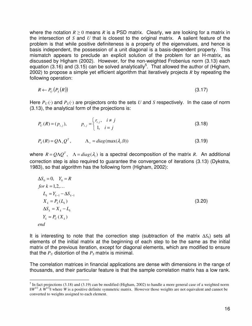
where the notation R ≥ 0 means R is a PSD matrix. Clearly, we are looking for a matrix in the intersection of S and U that is closest to the original matrix. A salient feature of the problem is that while positive definiteness is a property of the eigenvalues, and hence is basis independent, the possession of a unit diagonal is a basis-dependent property. This mismatch appears to preclude an explicit solution of the problem for an H-matrix, as discussed by Higham (2002). However, for the non-weighted Frobenius norm (3.13) each equation (3.16) and (3.15) can be solved analytically5. That allowed the author of (Higham, 2002) to propose a simple yet efficient algorithm that iteratively projects R by repeating the following operation:
( )( )RPPR SU← (3.17)
Here PU (·) and PS (·) are projectors onto the sets U and S respectively. In the case of norm (3.13), the analytical form of the projections is:
=
≠==
ji
jirppRP
ji
jijiU,1
,),()(
,
,, (3.18)
))0,(max(,)( i
T
S diagQQRP λ=ΛΛ= ++ (3.19)
where )(, i
TdiagQQR λ=ΛΛ= is a spectral decomposition of the matrix R. An additional
correction step is also required to guarantee the convergence of iterations (3.13) (Dykstra, 1983), so that algorithm has the following form (Higham, 2002):
end
XPY
LXS
LPX
SYL
kfor
RYS
kUk
kkk
kSk
kkk
)(
)(
,2,1
,0
11
00
=
−=∆
=
∆−=
=
==∆
−−
K
(3.20)
It is interesting to note that the correction step (subtraction of the matrix ∆Sk) sets all elements of the initial matrix at the beginning of each step to be the same as the initial matrix of the previous iteration, except for diagonal elements, which are modified to ensure that the PU distortion of the PS matrix is minimal. The correlation matrices in financial applications are dense with dimensions in the range of thousands, and their particular feature is that the sample correlation matrix has a low rank.
5 In fact projections (3.18) and (3.19) can be modified (Higham, 2002) to handle a more general case of a weighted norm
||W1/2
A W1/2
|| where W is a positive definite symmetric matrix. However those weights are not equivalent and cannot be
converted to weights assigned to each element.
17
This allows to compute PS (Lk) at a much lower cost than that of computing the complete
eigensystem of Lk for each iteration. It is sufficient to compute only positive eigenvalues λj and corresponding orthonormal eigenvectors qj and then take the truncated sum:
∑>
=0
)(i
T
iiikS qqLPλ
λ
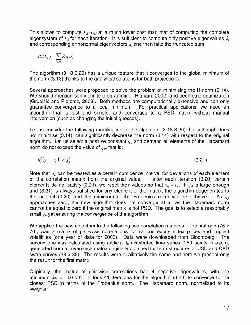
The algorithm (3.18-3.20) has a unique feature that it converges to the global minimum of the norm (3.13) thanks to the analytical solutions for both projections. Several approaches were proposed to solve the problem of minimising the H-norm (3.14). We should mention semidefinite programming (Higham, 2002) and geometric optimization (Grubišić and Pietersz, 2003). Both methods are computationally extensive and can only guarantee convergence to a local minimum. For practical applications, we need an algorithm that is fast and simple, and converges to a PSD matrix without manual intervention (such as changing the initial guesses). Let us consider the following modification to the algorithm (3.18-3.20) that although does not minimise (3.14), can significantly decrease the norm (3.14) with respect to the original
algorithm. Let us select a positive constant qρ and demand all elements of the Hadamard
norm do not exceed the value of qρ, that is:
( ) 222
ρqryh ijijij <− (3.21)
Note that qρ can be treated as a certain confidence interval for deviations of each element of the correlation matrix from the original value. If after each iteration (3.20) certain
elements do not satisfy (3.21), we reset their values so that yij = rij. If qρ is large enough and (3.21) is always satisfied for any element of the matrix, the algorithm degenerates to
the original (3.20) and the minimum of the Frobenius norm will be achieved. As qρ approaches zero, the new algorithm does not converge at all as the Hadamard norm cannot be equal to zero if the original matrix is not PSD. The goal is to select a reasonably
small qρ yet ensuring the convergence of the algorithm.
We applied the new algorithm to the following two correlation matrices. The first one (76 × 76), was a matrix of pair-wise correlations for various equity index prices and implied volatilities (one year of data for 2003). Data were downloaded from Bloomberg. The second one was calculated using artificial t3 distributed time series (250 points in each), generated from a covariance matrix originally obtained for term structures of USD and CAD
swap curves (38 × 38). The results were qualitatively the same and here we present only the result for the first matrix. Originally, the matrix of pair-wise correlations had 4 negative eigenvalues, with the
minimum λ76 = –0.01733. It took 41 iterations for the algorithm (3.20) to converge to the closest PSD in terms of the Frobenius norm. The Hadamard norm, normalized to its weights:
18
∑∑
∑∑=
i j
ij
i j
ijij
normH h
ah
A 2
22
2
,||||
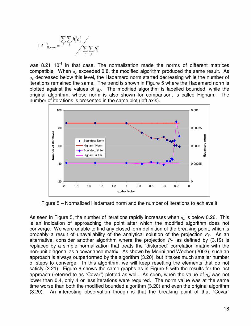
was 8.21 10-4 in that case. The normalization made the norms of different matrices
compatible. When qρ exceeded 0.8, the modified algorithm produced the same result. As
qρ decreased below this level, the Hadamard norm started decreasing while the number of iterations remained the same. The trend is shown in Figure 5 where the Hadamard norm is
plotted against the values of qρ. The modified algorithm is labelled bounded, while the original algorithm, whose norm is also shown for comparison, is called Higham. The number of iterations is presented in the same plot (left axis).
0
0.00025
0.0005
0.00075
0.001
00.20.40.60.811.21.41.61.82
q_rho factor
Had
am
ard
no
rm
20
40
60
80
100
Nu
mb
er
of
itera
tio
ns
Bounded: Norm
Higham: Norm
Bounded: # Iter.
Higham: # Iter.
Figure 5 – Normalized Hadamard norm and the number of iterations to achieve it
As seen in Figure 5, the number of iterations rapidly increases when qρ is below 0.26. This is an indication of approaching the point after which the modified algorithm does not converge. We were unable to find any closed form definition of the breaking point, which is probably a result of unavailability of the analytical solution of the projection PS. As an alternative, consider another algorithm where the projection PS as defined by (3.19) is replaced by a simple normalization that treats the “disturbed” correlation matrix with the non-unit diagonal as a covariance matrix. As shown by Morini and Webber (2003), such an approach is always outperformed by the algorithm (3.20), but it takes much smaller number of steps to converge. In this algorithm, we will keep resetting the elements that do not satisfy (3.21). Figure 6 shows the same graphs as in Figure 5 with the results for the last
approach (referred to as “Covar”) plotted as well. As seen, when the value of qρ was not lower than 0.4, only 4 or less iterations were required. The norm value was at the same time worse than both the modified bounded algorithm (3.20) and even the original algorithm (3.20). An interesting observation though is that the breaking point of that “Covar”
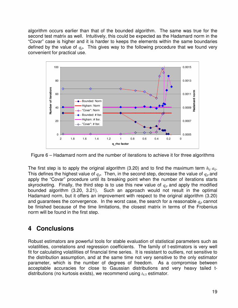
19
algorithm occurs earlier than that of the bounded algorithm. The same was true for the second test matrix as well. Intuitively, this could be expected as the Hadamard norm in the “Covar” case is higher and it is harder to keeps the elements within the same boundaries
defined by the value of qρ. This gives way to the following procedure that we found very convenient for practical use.
0.0005
0.0007
0.0009
0.0011
0.0013
0.0015
00.20.40.60.811.21.41.61.82
q_rho factor
Had
am
ard
no
rm
0
20
40
60
80
100
Nu
mb
er
of
itera
tio
ns
Bounded: Norm
Higham: Norm
"Covar": Norm
Bounded: # Iter.
Higham: # Iter.
"Covar": # Iter.
Figure 6 – Hadamard norm and the number of iterations to achieve it for three algorithms
The first step is to apply the original algorithm (3.20) and to find the maximum term hij aij.
This defines the highest value of qρ. Then, in the second step, decrease the value of qρ and apply the “Covar” procedure until its breaking point when the number of iterations starts
skyrocketing. Finally, the third step is to use this new value of qρ and apply the modified bounded algorithm (3.20, 3.21). Such an approach would not result in the optimal Hadamard norm, but it offers an improvement with respect to the original algorithm (3.20)
and guarantees the convergence. In the worst case, the search for a reasonable qρ cannot be finished because of the time limitations, the closest matrix in terms of the Frobenius norm will be found in the first step.
4 Conclusions Robust estimators are powerful tools for stable evaluation of statistical parameters such as volatilities, correlations and regression coefficients. The family of t-estimators is very well fit for calculating volatilities of financial time series. It is resistant to outliers, not sensitive to the distribution assumption, and at the same time not very sensitive to the only estimator parameter, which is the number of degrees of freedom. As a compromise between acceptable accuracies for close to Gaussian distributions and very heavy tailed t-distributions (no kurtosis exists), we recommend using t4.5 estimator.
20
The most stable and accurate estimates of a pair-wise correlation can be obtained using Kendall’s tau. Pair-wise correlations do not guarantee a positive definite matrix. The correlation matrix can be “improved” using an iterative procedure, which involves only eigenvalue decomposition if all correlations are given equal weights, or non-linear optimization in each step if the accuracy of each pair-wise correlation is incorporated.
5 References Huber, P.J. (1981), “Robust Statistics,” New York: Wiley. Press, W.H., Teukolsky, S.A. Vetterling, W.T. and Flannery, B.P. (1992), “Numerical
Recipes in C: The Art of Scientific Computing,” 2nd edition, Cambridge University Press.
Croux, C. and Rousseeuw, P.J. (1992), “Time-efficient algorithms for two highly robust estimators of scale,” in Computational Statistics, vol. 1, eds. Y. Dodge and J. Whittaker, Heidelberg: Physika-Verlag, 411-428.
Randal, J.A. (2002), “Robust volatility estimation and analysis of the leverage effect,” PhD Thesis, Victoria University of Wellington, New Zeeland.
Lally, M.T., Randal, J.A. and Thomson, P.J. (2001), “Non–parametric volatility estimation,” Proceedings of the 2nd International Symposium on Business and Industrial Statistics, Yokohama, Japan, 201–210.
Cramér, H. (1999), “Mathematical Methods of Statistics,” Princeton: Princeton University Press.
Mudrov, V.I and Kushko, V.L (1976), “Methods of Data Processing” (in Russuan: “Metody Obrabotki Rezul’tatov Izmerenij”), Moscow: Soviet Radio.
Kendall, M.G. and Gibbons, J.D. (1990), “Rank Correlation Methods,” 5th edition, London: Oxford University Press.
Lindskog, F. (2000), “Linear correlation estimation,” Research report, RiskLab Switzerland. Alqallaf, F.A., Konis, K.P., Martin, R.D. and Zamar, R.H. (2002), "Scalable robust
covariance and correlation estimates for data mining," Proceedings of the 7th ACM SIGKDD International Conference on Knowledge Discovery and Data Mining, Edmonton, Alberta, 14-23.
Higham, N.J. (2002), “Computing the nearest correlation matrix – a problem from finance,” IMA Journal of Numerical Analysis, 22, 329-343.
Dykstra, R.L. (1983), “An algorithm for restricted least squares regression,” J. Amer. Stat. Assoc., 78, 837-842.
Grubišić, I. and Pietersz, R. (2003), “Efficient Rank Reduction of Correlation Matrices,” working paper.
Morini, M and Webber, N. (2003), “A fast and accurate iterative algorithm to reduce the rank of a correlation matrix in financial modelling,” working paper, presented at V Workshop di Finanza Quantitativa, Siena, January 29-30, 2004.
21
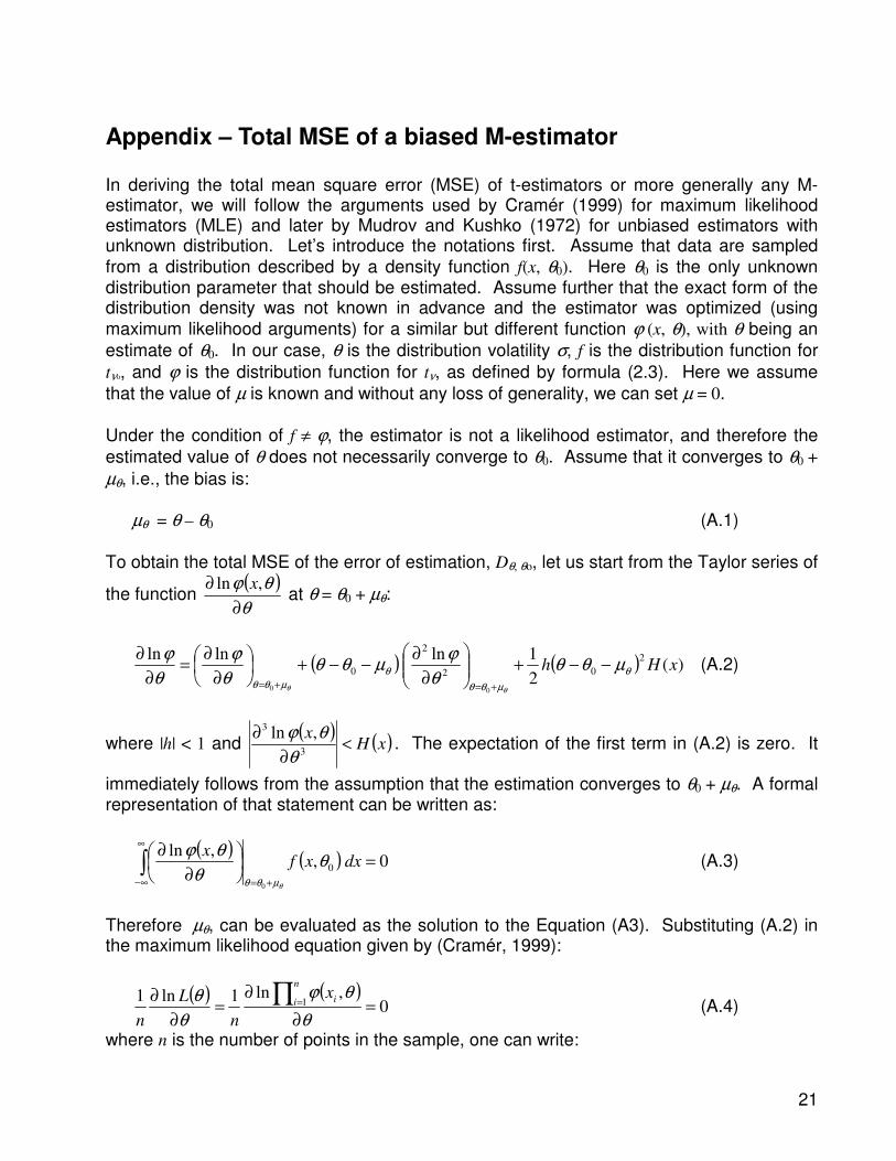
Appendix – Total MSE of a biased M-estimator In deriving the total mean square error (MSE) of t-estimators or more generally any M-estimator, we will follow the arguments used by Cramér (1999) for maximum likelihood estimators (MLE) and later by Mudrov and Kushko (1972) for unbiased estimators with unknown distribution. Let’s introduce the notations first. Assume that data are sampled
from a distribution described by a density function f(x, θ0). Here θ0 is the only unknown distribution parameter that should be estimated. Assume further that the exact form of the distribution density was not known in advance and the estimator was optimized (using
maximum likelihood arguments) for a similar but different function ϕ (x, θ), with θ being an
estimate of θ0. In our case, θ is the distribution volatility σ, f is the distribution function for
tνo, and ϕ is the distribution function for tν, as defined by formula (2.3). Here we assume
that the value of µ is known and without any loss of generality, we can set µ = 0.
Under the condition of f ≠ ϕ, the estimator is not a likelihood estimator, and therefore the
estimated value of θ does not necessarily converge to θ0. Assume that it converges to θ0 +
µθ, i.e., the bias is:
µθ = θ – θ0 (A.1)
To obtain the total MSE of the error of estimation, Dθ, θo, let us start from the Taylor series of
the function ( )θ
θϕ
∂
∂ ,ln x at θ = θ0 + µθ:
( ) ( ) )(2
1lnlnln 2
02
2
0
00
xHh θ
µθθ
θ
µθθ
µθθθ
ϕµθθ
θ
ϕ
θ
ϕ
θθ
−−+
∂
∂−−+
∂
∂=
∂
∂
+=+=
(A.2)
where |h| < 1 and ( ) ( )xHx
<∂
∂3
3 ,ln
θ
θϕ. The expectation of the first term in (A.2) is zero. It
immediately follows from the assumption that the estimation converges to θ0 + µθ. A formal representation of that statement can be written as:
( ) ( ) 0,,ln
0
0
=
∂
∂∫∞
∞− +=
dxxfx
θθ
θϕ
θµθθ
(A.3)
Therefore µθ, can be evaluated as the solution to the Equation (A3). Substituting (A.2) in the maximum likelihood equation given by (Cramér, 1999):
( ) ( )0
,ln1ln1 1 =∂
∂=
∂
∂ ∏ =
θ
θϕ
θ
θn
i ix
n
L
n (A.4)
where n is the number of points in the sample, one can write:
22
( ) ( ) ( ) ( )∑∑∑
== +== +=
−−+
∂
∂−−+
∂
∂ n
i
i
n
i
in
i
i xHn
hx
n
x
n 1
2
0
12
2
0
1
)(2
,ln,ln1
00
θ
µθθ
θ
µθθ
µθθ
θ
θϕµθθ
θ
θϕ
θθ
( ) ( )0
22
2
0100 =
−−+−−+= B
hBB θ
θ
µθθµθθ (A.5)
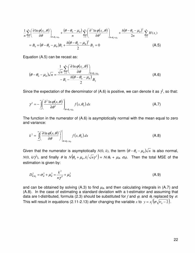
Equation (A.5) can be recast as:
( )
( )
( )2
01
1
0
2
,ln1
0
Bh
B
x
nn
n
i
i
θ
µθθ
θ µθθ
θ
θϕ
µθθ θ
−−−−
∂
∂
=−−
∑= +=
(A.6)
Since the expectation of the denominator of (A.6) is positive, we can denote it as γ2, so that:
( ) ( )∫∞
∞− +=
∂
∂−= dxxf
x02
22 ,
,ln
0
θθ
θϕγ
θµθθ
(A.7)
The function in the numerator of (A.6) is asymptotically normal with the mean equal to zero and variance:
( ) ( )∫∞
∞− +=
∂
∂= dxxf
xk 0
2
2 ,,ln
0
θθ
θϕ
θµθθ
(A.8)
Given that the numerator is asymptotically N(0, k), the term ( ) nθµθθ −− 0 is also normal,
N(0, k/γ2), and finally θ is ( )2
0 , γµθ θ nkN + = N(θ0 + µθ, σθ). Then the total MSE of the
estimation is given by:
2
4
2222
, 0 θθθθθ µγ
µσ +=+=n
kD (A.9)
and can be obtained by solving (A.3) to find µθ, and then calculating integrals in (A.7) and (A.8). In the case of estimating a standard deviation with a t-estimator and assuming that
data are t-distributed, formula (2.3) should be substituted for f and ϕ, and θ0 replaced by σ.
This will result in equations (2.11-2.13) after changing the variable x to ( )20 −= νσxy .