Robust Investment Management with Uncertainty in Fund

Managers’ Asset Allocation

Yang Dong∗ Aurelie Thiele †

April 2014, revised December 2014

Abstract

We consider a problem where an investment manager must allocate an available budget among a

set of fund managers, whose asset class allocations are not precisely known to the investment manager.

In this paper, we propose a robust framework that takes into account the uncertainty stemming from

the fund managers’ allocation, as well as the more traditional uncertainty due to uncertain asset class

returns, in the context of manager selection and portfolio management. We assume that only bounds on

the fund managers’ holdings (expressed as fractions of the portfolio) are available, and fractions must

sum to 1 for each fund manager. We define worst-case risk as the largest variance attainable by the

investment manager’s portfolio over that uncertainty set. We propose two exact approaches (of different

complexity) and a heuristic one to solve the problem efficiently. Numerical experiments suggest that our

robust model provides better protection against risk than the nominal model when the fund managers’

allocations are not known precisely.

1 Motivation and Literature Review

Institutional investors, such as pension funds, university endowments and insurance companies, actively

manage their portfolio by investing money in outside fund managers with the expectation of generating

superior returns while keeping risk at an acceptable level. Fund managers might have quite different risk

and return profiles regarding their strategy and investment process, and the investment manager (institutional

investor) must decide how to allocate his budget among them given a high-level idea of each fund’s strategy,∗Senior Quantitative Analyst, JP Morgan, New York, NY yad210@lehigh.edu This research was done while the first author was

a doctoral student at Lehigh University.†Visiting Associate Professor, M.I.T. Sloan School of Management, Cambridge, MA, USA and Associate Professor, Lehigh

University, Department of Industrial and Systems Engineering, Bethlehem, PA, USA aut204@lehigh.edu

1

as expressed in its prospectus, but without knowing the fund managers’ allocation exactly. While a rich

body of literature exists on portfolio management, starting with the pioneering work of Markowitz [27]

on mean-variance allocation and while the issue of uncertainty in stocks’ expected returns and covariances

has received significant attention in the operations research community, the double uncertainty – from an

institutional investor’s perspective – stemming from both asset returns and managers’ allocation, has to the

best of our knowledge received no attention at all in terms of quantitative decision-making models. The

purpose of this paper is to address such a gap.

1.1 Literature review

Performance attribution

The reader is referred to Maginn et al. [25] and Swensen [34] for introductions to the management of invest-

ment portfolios. Methods developed in finance to explain fund managers’ performance versus a benchmark

index such as the return of the S&P 500 are called fund performance attribution analysis. Previous research

has focused on evaluating fund managers’ skills by decomposing observed fund returns into several com-

ponents. Brinson et al. [9] suggest a method to decompose the manager’s added value into three parts: (1)

asset allocation, (2) stock selection and (3) intersection between the two. This method has the following

drawbacks: it does not incorporate the fact that over-weighting a portfolio in a negative market that has

outperformed the overall benchmark should still have a positive effect, and it fails to distinguish between

the static manager and the dynamic manager, who is trying to capture opportunity when the market is up

in one sector and thus over-weighs his portfolio in that sector. Lo [24] and Hsu and Myers [20] both pro-

pose approaches to capture the static and dynamic contributions of a fund manager’s performance. In their

models, weights are considered to be a stochastic process as opposed to fixed parameters. The dynamic

component is measured by the sum of the covariances between returns and portfolio weights. The fund

return is split into an active management component (reflecting the fund manager’s skill) and a passive man-

agement component (reflecting stock performance). Reed et al. [29] investigate downside risk management

from institutional investors’ perspectives and present a decomposition that separate the risk contributions of

individual securities from that of investment decisions.

Fund returns can also be decomposed into systematic and unsystematic components. Such a decom-

position was first presented in the Capital Asset Pricing Model, where the unsystematic component can be

considered as the value added by the manager’s performance. It was further developed in Treynor [36],

Sharpe [31], Jensen [21] and Jensen [22], who also provide risk-adjusted performance measures such as

the Sharpe Ratio, Treynor Ratio and Information Ratio to evaluate the fund manager’s performance. These

2

measures are all static measures, based on the characteristics of returns in a single time period. Treynor and

Mazuy [38] propose a method to measure the fund managers’s ability to capture the up market by introduc-

ing the quadratic term in the excess return (Rmt − Rf )2. Arnott et al. [1] and Treynor [37] also consider

the covariance between portfolio weights and returns but this is only discussed in the context of providing

capitalization-indifferent equity market indexes that deliver superior mean-variance performance. Grinblatt

and Titman [19] point out that the positive covariance between portfolio weights and returns should bring

benefit to investors, and propose a measure that exhibits this property.

Decentralized investment management

A research area related to the present paper is decentralized investment management, pioneered by Sharpe

[32]. Barry and Starks [2] focus on risk-sharing as a reason for the investor’s decision to employ multi-

ple managers and provide conditions under which a multi-manager allocation is optimal when managers’

specialization and diversification are not motives for the use of multiple managers. Elton and Gruber [16]

investigate how to set up a structure that would lead, in a decentralized investment situation, to the opti-

mal portfolio for the centralized decision-maker. Specifically, the authors list the following four tasks for

a centralized decision-maker and explain that their paper focuses on the first two: “(1) decide how much

to invest in each portfolio, (2) give the outside managers instructions that will result in their making opti-

mum security allocations from the point of view of the overall plan, (3) design incentive systems so that

the managers will behave optimally, and (4) evaluate and select the portfolio managers.” The authors derive

conditions under which a centralized decision-maker can form an optimal overall portfolio by employing

outside portfolio managers. Two key factors are whether the centralized manager assigns informative value

to negative alphas when there are multiple active managers and whether short sales are allowed.

Van Binsbergen et al. [40] also study a problem where a centralized decision-maker employs multiple

asset managers. In their setting, the decision-maker is uncertain about the portfolio managers’ risk appetites.

The authors show how a well-chosen unconditional linear performance benchmark can better align the in-

centive between the centralized decision-maker and the portfolio managers, when considering two asset

classes (bonds and stocks) and three assets per class (for bonds: government-rated bonds, Baa-rated corpo-

rate bonds and Aaa-rated corporate bonds, and for stocks: growth stocks, intermediate and value stocks).

Blake et al. [8] provide an empirical study in the pension fund industry, for which they document two im-

portant trends: the switch from generalist balanced managers to more specialized ones and, within asset

classes, the switch from a single-manager situation to settings with multiple competing managers.

These approaches offer investors valuable ways to evaluate fund managers, but do not address the prob-

lem of creating a portfolio in presence of uncertainty on the fund managers’ allocation.

3

Parameter uncertainty

Parameter uncertainty in classical mean-variance portfolio management has been studied extensively (al-

though not specifically in a decentralized investment management context) since Chopra and Ziemba [11]

documented the impact of mean and covariance estimation errors on mean-variance portfolios. Techniques

suggested to mitigate the impact of such errors include stochastic optimization (Pflug and Wozabal [28]), ro-

bust statistic models (DeMiguel and Nogales [13], Garlappi et al. [17]), shrinkage (a method that transforms

the sample covariance matrix by pulling the more extreme coefficients toward central values, see DeMiguel

et al. [14] and Ledoit and Wolf [23]) and robust optimization, which models uncertain parameters using

range forecasts and optimizes the worst-case objective, here, minimizes the worst-case variance, with the

worst case being computed over that uncertainty set (Ben-Tal et al. [3], Ben-Tal et al. [4], Bertsimas et al.

[6]). Applications of robust optimization to classical portfolio management with uncertain parameters have

been presented in Ben-Tal et al. [3] and Goldfarb and Iyengar [18], among others. In particular, Goldfarb

and Iyengar [18] investigate robust mean-variance portfolio selection problems under a specific uncertainty

structure that leads to second-order cone problems and thus can be solved efficiently. Portfolio optimization

with uncertainty over a set of distributions has also been studied, for instance in El-Ghaoui et al. [15], which

assumes that only bounds on the mean and covariance matrix are available in the context of worst-case

value-at-risk optimization, and in Delage and Ye [12], which incorporates ambiguity in both the distribution

and its moments in a tractable formulation applied to portfolio selection.

A key technique we will use is delayed constraint generation to address the issue of scale in our robust

formulations. Delayed constraint generation was first introduced in Benders [5]. The use of this technique

in the context of tractable robust formulations is for instance presented in Thiele et al. [35] and Zeng [41].

Important variations on Benders’ decomposition, still for robust optimization but in the context of inventory

management with basestock levels, are described in Bienstock and Ozbay [7]. Further, Zhang [42] presents

delayed constraint generation for multi-period pricing of perishable products under uncertainty.

1.2 Contributions

In this paper, our goal is to provide an optimization approach to construct a portfolio of funds for the

investment manager while taking into account that the funds’ tactical allocation is not precisely known. The

methodology we will use to achieve that goal is robust optimization. We will investigate this methodology

in the context of the well-known mean-variance framework, or Markowitz framework, where we seek to

minimize worst-case variance of the investment manager’s portfolio (with the worst case computed over the

parameters’ uncertainty set) subject to a constraint on the expected return. Short sales are not allowed in

4

our model; they are usually prohibited in university endowment funds. Further, this allows the investment

manager further insights into the fund managers he selects, as defined by non-negative fund investments.

(In the presence of short sales, all fund managers are always selected but the allocation into their fund may

be negative.) Uncertainty in finance has been well studied in the context of stock returns, but not regarding

the asset allocation of fund managers. Our paper presents a new framework that extends the traditional

mean-variance model to the problem faced by the investment (or fund of funds) manager. We also propose

an efficient algorithm to solve the problem and provide insights into the fund managers who are chosen by

the investment manager. Our numerical results indicate that uncertainty in managers’ asset allocation does

affect the investment manager’s optimal strategy, and suggest that our robust model protects the investment

manager against (fund managers’) allocation risk.

Structure of the Paper

We present the general framework of the robust manager selection model in Section 2. In Section 3, we

propose two algorithms for solving this problem. In Section 4, we apply the two proposed approaches to the

robust model in numerical experiments and compare results with the nominal model. A heuristic method

is also presented in order to solve the problem efficiently. Finally, Section 5 contains some concluding

remarks.

2 Robust Fund Manager Selection

2.1 Problem Setup

We seek to minimize the worst-case portfolio risk (variance) of the investment manager, while guaranteeing

that expected return achieves or beats a certain benchmark. Investment managers typically express their

portfolio holdings in terms of broad asset classes rather than specific assets; this is therefore the practice that

we will follow throughout this paper. From a mathematical standpoint, it has also the advantage of keeping

the problem size smaller, since assets are grouped into a smaller number of asset classes. Each manager’s

allocation in each asset class is subject to ambiguity but is known to fall within a certain range. Non-negative

allocation weights model that short sales are not allowed. The fund managers selected by the model will be

those for whom the investment manager’s allocation has strictly positive weights.

We will use the following notation:

Decision Variables

xi: allocation in fund manager i

5

Parameters related to fund managers’ allocationswij : (uncertain) allocation of manager i in asset class j

w+ij : upper bound of allocation of manager i in asset class j

w−ij : lower bound of allocation of manager i to asset class j

wij : nominal allocation of manager i to asset class j

Other parametersn: number of fund managers

m: number of asset classes

rj : expected return from asset class j

cov(rj , rl) : covariance between the returns of asset class j and asset class l

τ : portfolio return benchmark.

2.2 Formulation

The problem without uncertainty on the fund managers’ allocation, in the classical Markowitz framework,

can be formulated as:

minxn∑

i=1

m∑j=1

n∑k=1

m∑l=1

wijwkl cov(rj , rl)xixk (1)

s.t.n∑

i=1

xi = 1

n∑i=1

m∑j=1

wijrj xi ≥ τ

xi ≥ 0,∀i

When there is uncertainty on the fund managers’ allocation, Problem (1) becomes:

6

minx maxωn∑

i=1

m∑j=1

n∑k=1

m∑l=1

wijwkl cov(rj , rl)xixk (2)

s.t.m∑j=1

wij = 1,∀i

w−ij ≤ wij ≤ w+ij ,∀i, j

s.t.n∑

i=1

xi = 1

n∑i=1

m∑j=1

wijrj xi ≥ τ

xi ≥ 0, ∀i

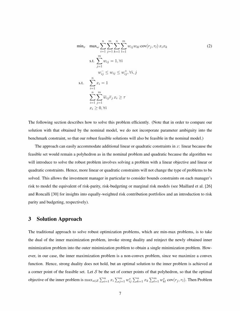
The following section describes how to solve this problem efficiently. (Note that in order to compare our

solution with that obtained by the nominal model, we do not incorporate parameter ambiguity into the

benchmark constraint, so that our robust feasible solutions will also be feasible in the nominal model.)

The approach can easily accommodate additional linear or quadratic constraints in x: linear because the

feasible set would remain a polyhedron as in the nominal problem and quadratic because the algorithm we

will introduce to solve the robust problem involves solving a problem with a linear objective and linear or

quadratic constraints. Hence, more linear or quadratic constraints will not change the type of problems to be

solved. This allows the investment manager in particular to consider bounds constraints on each manager’s

risk to model the equivalent of risk-parity, risk-budgeting or marginal risk models (see Maillard et al. [26]

and Roncalli [30] for insights into equally-weighted risk contribution portfolios and an introduction to risk

parity and budgeting, respectively).

3 Solution Approach

The traditional approach to solve robust optimization problems, which are min-max problems, is to take

the dual of the inner maximization problem, invoke strong duality and reinject the newly obtained inner

minimization problem into the outer minimization problem to obtain a single minimization problem. How-

ever, in our case, the inner maximization problem is a non-convex problem, since we maximize a convex

function. Hence, strong duality does not hold, but an optimal solution to the inner problem is achieved at

a corner point of the feasible set. Let S be the set of corner points of that polyhedron, so that the optimal

objective of the inner problem is maxs∈S∑n

i=1 xi∑m

j=1wsij

∑nk=1 xk

∑ml=1w

skl cov(rj , rl). Then Problem

7

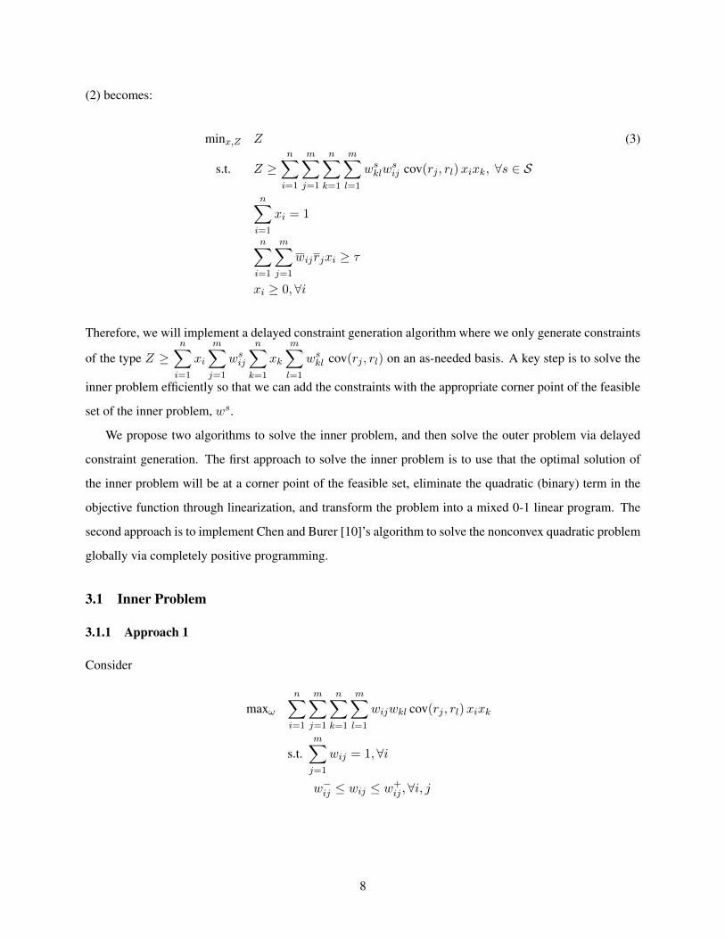
(2) becomes:

minx,Z Z (3)

s.t. Z ≥n∑

i=1

m∑j=1

n∑k=1

m∑l=1

wsklw

sij cov(rj , rl)xixk, ∀s ∈ S

n∑i=1

xi = 1

n∑i=1

m∑j=1

wijrjxi ≥ τ

xi ≥ 0, ∀i

Therefore, we will implement a delayed constraint generation algorithm where we only generate constraints

of the type Z ≥n∑

i=1

xi

m∑j=1

wsij

n∑k=1

xk

m∑l=1

wskl cov(rj , rl) on an as-needed basis. A key step is to solve the

inner problem efficiently so that we can add the constraints with the appropriate corner point of the feasible

set of the inner problem, ws.

We propose two algorithms to solve the inner problem, and then solve the outer problem via delayed

constraint generation. The first approach to solve the inner problem is to use that the optimal solution of

the inner problem will be at a corner point of the feasible set, eliminate the quadratic (binary) term in the

objective function through linearization, and transform the problem into a mixed 0-1 linear program. The

second approach is to implement Chen and Burer [10]’s algorithm to solve the nonconvex quadratic problem

globally via completely positive programming.

3.1 Inner Problem

3.1.1 Approach 1

Consider

maxωn∑

i=1

m∑j=1

n∑k=1

m∑l=1

wijwkl cov(rj , rl)xixk

s.t.m∑j=1

wij = 1, ∀i

w−ij ≤ wij ≤ w+ij ,∀i, j

8

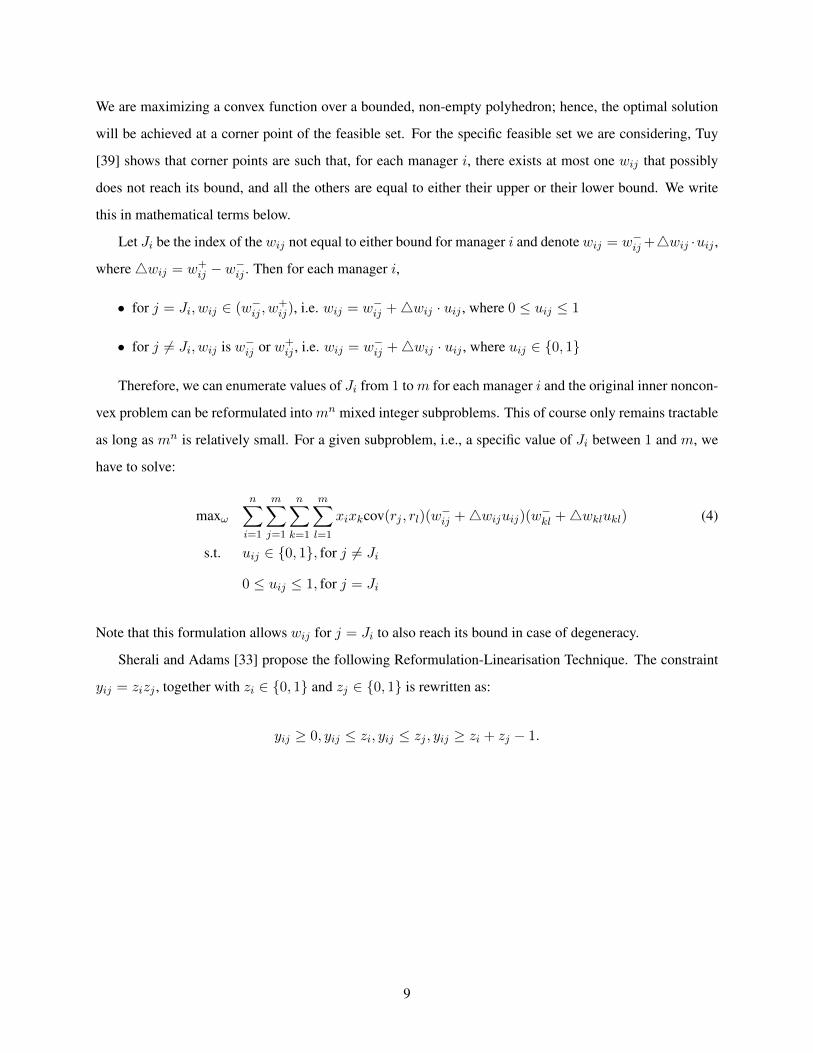
We are maximizing a convex function over a bounded, non-empty polyhedron; hence, the optimal solution

will be achieved at a corner point of the feasible set. For the specific feasible set we are considering, Tuy

[39] shows that corner points are such that, for each manager i, there exists at most one wij that possibly

does not reach its bound, and all the others are equal to either their upper or their lower bound. We write

this in mathematical terms below.

Let Ji be the index of the wij not equal to either bound for manager i and denote wij = w−ij +4wij ·uij ,

where4wij = w+ij − w

−ij . Then for each manager i,

• for j = Ji, wij ∈ (w−ij , w+ij), i.e. wij = w−ij +4wij · uij , where 0 ≤ uij ≤ 1

• for j 6= Ji, wij is w−ij or w+ij , i.e. wij = w−ij +4wij · uij , where uij ∈ {0, 1}

Therefore, we can enumerate values of Ji from 1 tom for each manager i and the original inner noncon-

vex problem can be reformulated into mn mixed integer subproblems. This of course only remains tractable

as long as mn is relatively small. For a given subproblem, i.e., a specific value of Ji between 1 and m, we

have to solve:

maxωn∑

i=1

m∑j=1

n∑k=1

m∑l=1

xixkcov(rj , rl)(w−ij +4wijuij)(w

−kl +4wklukl) (4)

s.t. uij ∈ {0, 1}, for j 6= Ji

0 ≤ uij ≤ 1, for j = Ji

Note that this formulation allows wij for j = Ji to also reach its bound in case of degeneracy.

Sherali and Adams [33] propose the following Reformulation-Linearisation Technique. The constraint

yij = zizj , together with zi ∈ {0, 1} and zj ∈ {0, 1} is rewritten as:

yij ≥ 0, yij ≤ zi, yij ≤ zj , yij ≥ zi + zj − 1.

9

Substituting uijukl by vijkl, Problem (4) can therefore be reformulated as:

maxωn∑

i=1

m∑j=1

n∑k=1

m∑l=1

xixkcov(rj , rl)(w−ijw

−kl + 2w−kl 4 wij · uij +4wij 4 wkl · vijkl

)(5)

s.t. vijkl ≤ uij , ∀i, j

vijkl ≤ ukl,∀k, l

vijkl ≥ uij + ukl − 1, ∀i, j, k, l

uij ∈ {0, 1}, for j 6= Ji, ∀i

0 ≤ uij ≤ 1, for j = Ji, ∀i.

3.1.2 Approach 2

Chen and Burer [10] propose a method to solve nonconvex quadratic programming problems to global op-

timality via completely positive programming. Their approach consists in employing a finite branch-and

bound (B&B) scheme, in which branching is based on the first-order KKT conditions and polyhedral-

semidominant relaxation are solved at each node of the (B&B) tree. The relaxations are derived from

completely positive and doubly nonnegative programming problems. The original quadratic programming

problem is reformulated as a quadratic programming problem with linear equality, nonnegativity and com-

plementarity constraints. Such a problem can be further reformulated as a completely positive programming

problem and relaxed to a doubly nonnegative programming problem.

3.2 Algorithm

As explained above, we solve the outer problem using delayed constraint generation. For the Sth iteration,

the outer problem can be formulated as:

minx,Z Z

s.t. Z ≥n∑

i=1

m∑j=1

n∑k=1

m∑l=1

wsijw

skl cov(rj , rl) xixk, ∀s = 1, 2, ...S (6)

n∑i=1

m∑j=1

xiwijrj ≥ τ,

n∑i=1

xi = 1

xi ≥ 0,∀i.

10

Therefore, we suggest the following algorithm to solve the investment manager’s problem, which converges

in a finite number of steps by definition of the master problem (3):

Algorithm 3.1 (Delayed constraint generation algorithm).

Step 1 Start with a feasible solution x ∈ X and set iteration number s := 0.

Step 2 Solve the inner problem (in w) with candidate solution xs as parameter using either Approach 1 or

Approach 2 and obtain optimal solution w, denoted ws+1.

Step 3 Solve the outer problem (6) (in x) with candidate weight ws+1 as parameter and obtain optimal

solution x, denoted xs+1. Set s := s+ 1.

Step 4 Repeat Steps 2 and 3 until there is no new delayed constraint to generate, i.e., the optimal w solution

outputted in Step 2 in step s has already been found in a previous step s′ < s and thus already appears

in the constraints of Problem (6).

4 Numerical Results

In this section, we present three experiments to illustrate our robust approach to the manager selection

problem with uncertainty in the asset allocations. The first set of experiment is to compare the performance

of the two approaches proposed in Section 3 to solve the inner problem and obtain corner points used in

the delayed constraint generation algorithm. The second experiment is to compare our robust approach with

the nominal approach from a risk standpoint. In the third experiment, we propose a heuristic algorithm

that improves solution time by pre-selecting a subset of the fund managers from the large candidate pool

into the robust manager selection model, and we compare the results of this heuristic method with the two

approaches we proposed in Section 3. The data was provided by the Lehigh University’s Investment Office,

including bounds on real funds’ allocations.

4.1 Comparison of the two approaches to solve the robust inner problem

In this set of experiments, we test the efficiency of the two approaches to solve the robust inner problem,

which are used to generate constraints in the delayed algorithm for the master problem: the MIP approach

and the Chen and Burer [10] approach. We test three instances: four managers with four asset classes,

six managers with six asset classes, and twelve managers with six asset classes. We observe that the first

approach (MIP approach) is more efficient than the second one when the problem size is small. However, as

11

the problem size increases, the computational advantage of the second approach becomes more significant.

When we consider the problem with twelve managers and six asset classes, the first approach needs to solve

612 independent mixed integer problems and the computations exceed the allowed time limit, while the

second approach can solve the problem in a reasonable time for this size. Tables 1-3 present the results as a

function of the expected-return benchmark τ , increasing from 0.15 onwards. Running times are expressed

in CPU seconds throughout. The worst variance of manager i is defined as the worst-case variance of his

portfolio’s return when his weights wij sum to 1 over all assets j and fall within the bounds [w−ij , w+ij ].

4.1.1 Four Managers with Four Asset Classes

Table 1: Four Managers with Four Asset Classes

worst variance nominal return 0.15 0.2 0.25 0.3 0.35 0.4 0.45

Manager 1 13.2566 0.0259 0 0 0 0 0 0 0

Manager 2 10.161 0.0227 0 0 0 0 0 0 0

Manager 3 11.2965 0.0457 0 0 0 0.17 0.4368 0.7 0.9632

Manager 4 7.645 0.0267 1 1 1 0.83 0.5632 0.3 0.0368

Variance (objective) 7.645 7.645 7.645 7.93 8.6456 9.6935 11.0762

Excess return 0.0117 0.0067 0.0017 0 0 0 0

Running Time Approach 1 (CPU sec.) 8.092 7.222 7.294 9.96 16.394 13.791 15.745

Running Time Approach 2 (CPU sec.) 13.274 12.95 15.055 25.6 27.134 26.487 44.493

We see from Table 1 that it is optimal for the investment manager to invest solely in the fund of Manager

4 for small values of τ (specifically, as long as the benchmark constraint is not tight). Once τ reaches 0.3,

the investment manager begins to diversify into the fund of Manager 3, and increases his allocation into that

fund until his allocation consists almost solely of Fund 3 for τ = 0.45. The MIP approach (Approach 1) is

initially about 39% faster than Approach 2, and for the largest value of τ considered, solves in about a third

of the time it takes for Approach 2 to terminate.

12

4.1.2 Six Managers with Six Asset Classes

Table 2: Six Managers with Six Asset Classes

worst var. nominal return 0.15 0.25 0.3 0.35 0.4 0.45 0.5 0.55

Manager 1 7.1842 0.0461 0.4303 0.4303 0.4303 0.4303 0.4937 0.3524 0.1778 0.0158

Manager 2 6.4727 0.0341 0.5697 0.5697 0.5697 0.5697 0.5063 0.3593 0.2284 0.0915

Manager 3 7.5552 0.0432 0 0 0 0 0 0 0 0

Manager 4 9.6658 0.0506 0 0 0 0 0 0 0 0

Manager 5 7.8224 0.0573 0 0 0 0 0 0.2883 0.5937 0.8927

Manager 6 10.3974 0.0525 0 0 0 0 0 0 0 0

Variance (obj) 6.2028 6.2028 6.2028 6.2028 6.2145 6.4857 6.9147 7.4998

Excess return 0.0242 0.0142 0.0092 0.0042 0 0 0 0

Running time Approach 1 (CPU sec.) 25768 26218 26423 26487 26407 26672 15859 28566

Running time Approach 2 (CPU sec.) 6848 7152 7242 7258 6870 9594 13233 16236

Table 2 shows increased diversification as τ increases, from investing in the funds of Managers 1 and 2 only

while the expected-return benchmark constraint is not tight, to investing in the funds of Managers 1, 2 and

5 with growing weight into Fund 5. We also observe that Approach 2 now takes less time to solve. For

small values of τ , Approach 1 takes about four times longer to terminate. For large values of τ , it takes

approximately 76% longer.

4.1.3 Twelve Managers with Six Asset Classes

The case with twelve managers and six asset classes is only solved using Approach 2, since Approach 1

runs into time limits. The investment manager initially allocates his budget between Managers 5, 10 and

12. As τ increases, Fund 4 is also chosen, and Fund 12 is taken out of the selection. Fund 6 is chosen for

some values of τ as well. The fact that some managers are never chosen will motivate the design of the

pre-selection heuristic we present in Section 4.3.

13

Table 3: Twelve Managers with Six Assets

worst

var.

nominal

return

0.15 0.2 0.25 0.3 0.35 0.4 0.45 0.5 0.55 0.6

Manager 1 8.921 0.0526 0 0 0 0 0 0 0 0 0 0

Manager 2 9.1132 0.0415 0 0 0 0 0 0 0 0 0 0

Manager 3 11.306 0.0461 0 0 0 0 0 0 0 0 0 0

Manager 4 8.9833 0.059 0 0 0 0 0 0.2253 0.431 0.622 0.8118 0.4923

Manager 5 7.6327 0.0316 0.6421 0.6421 0.6421 0.6421 0.6212 0.4865 0.3427 0.1858 0.0274 0

Manager 6 10.2603 0.0667 0 0 0 0 0 0 0.0005 0 0 0.4042

Manager 7 10.3677 0.029 0 0 0 0 0 0 0 0 0 0

Manager 8 8.8524 0.0201 0 0 0 0 0 0 0 0 0 0

Manager 9 9.9881 0.0145 0 0 0 0 0 0 0 0 0 0

Manager 10 10.031 0.0386 0.3468 0.3469 0.3468 0.3468 0.3051 0.2664 0.2258 0.1922 0.1608 0.1035

Manager 11 7.9499 0.031 0 0 0 0 0 0 0 0 0 0

Manager 12 8.885 0.0494 0.0111 0.011 0.0111 0.0111 0.0736 0.0218 0 0 0 0

Variance (obj) 6.8357 6.8357 6.8357 6.8357 6.8387 6.975 7.2184 7.6183 8.1685 8.9515

Excess return 0.0192 0.0142 0.0092 0.0042 0 0 0 0 0 0

Running time (CPU sec.) 30719 30599 29864 30553 31039 54754 55120 57464 48503 27397

4.2 Comparison between the nominal and the robust models

In this set of experiments, we compare our robust model with the nominal model where fund managers’

allocations are assumed equal to their nominal value. We then test the performance of the two models under

the nominal asset allocation scenario and the worst case asset allocation scenario. We also compare the

difference in the manager selection policy under the two models. The cases of six managers with six asset

classes and twelve managers with six asset classes are presented for illustration purposes.

4.2.1 Six managers with six asset classes

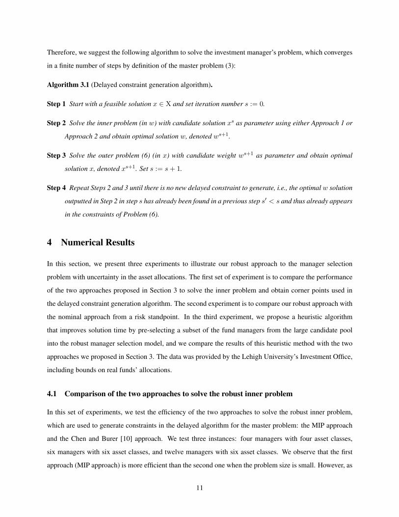
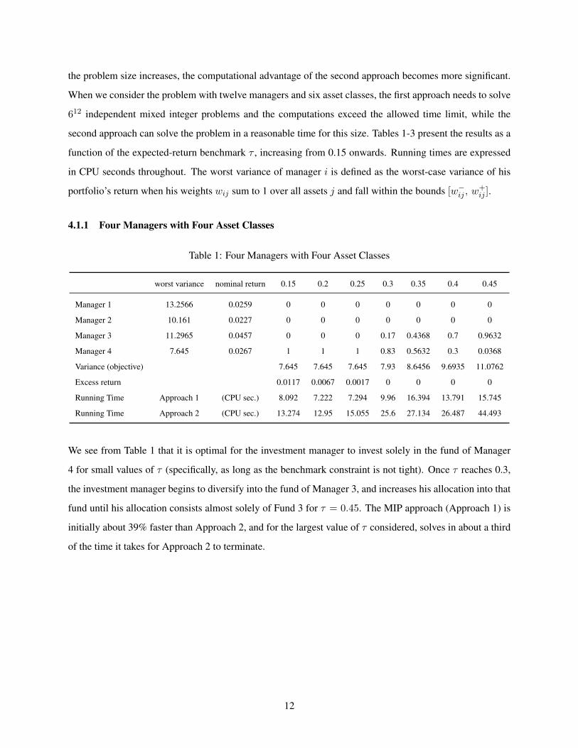
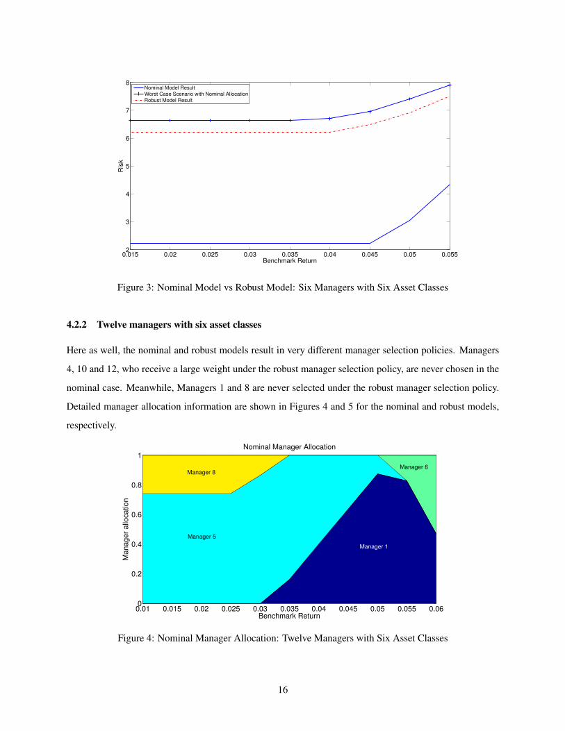
Figures 1 and 2 compare the optimal manager selection policy under the nominal and robust models, re-

spectively. In the nominal model, Manager 1 is always chosen for all values of the benchmark requirement

(parameter τ ), but with a decreasing weight as the benchmark return increases and Manager 5 is selected

with an increasing weight in the investment manager’s portfolio as the benchmark return exceed 0.045; how-

ever, in the robust model, Manager 1 has much less weight in the portfolio compared to his weight in the

nominal model. Manager 2, who is never selected in the nominal model, has an initially large weight in the

robust manager selection model, which decreases as τ increases.

14

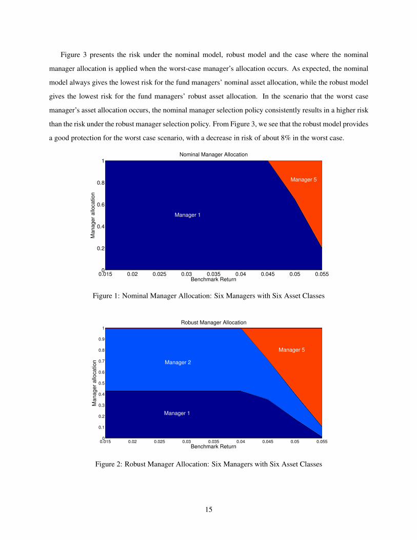
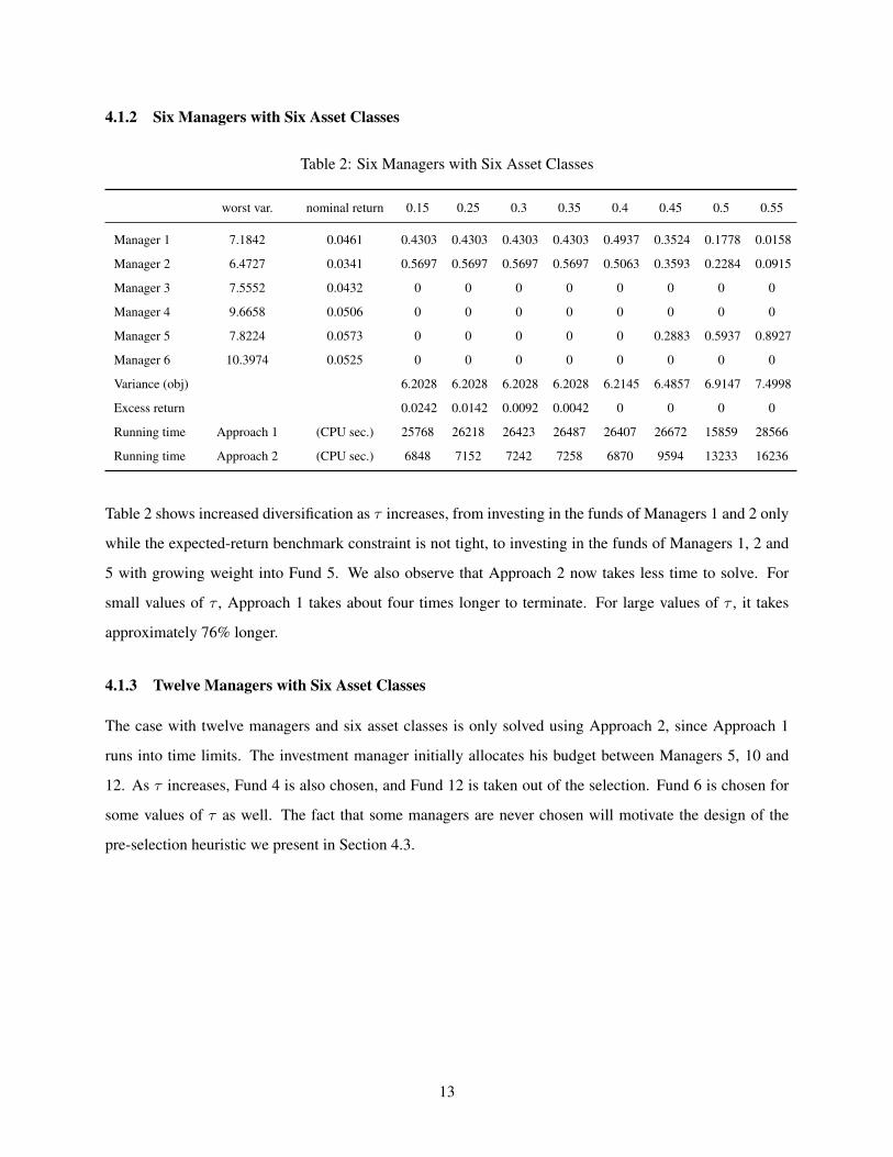
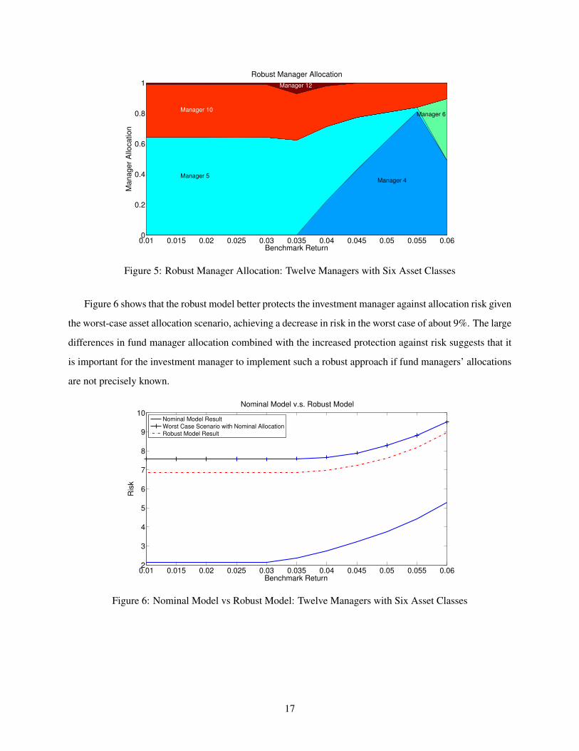
Figure 3 presents the risk under the nominal model, robust model and the case where the nominal

manager allocation is applied when the worst-case manager’s allocation occurs. As expected, the nominal

model always gives the lowest risk for the fund managers’ nominal asset allocation, while the robust model

gives the lowest risk for the fund managers’ robust asset allocation. In the scenario that the worst case

manager’s asset allocation occurs, the nominal manager selection policy consistently results in a higher risk

than the risk under the robust manager selection policy. From Figure 3, we see that the robust model provides

a good protection for the worst case scenario, with a decrease in risk of about 8% in the worst case.

0.015 0.02 0.025 0.03 0.035 0.04 0.045 0.05 0.0550

0.2

0.4

0.6

0.8

1Nominal Manager Allocation

Benchmark Return

Manager

allo

cation

Manager 5

Manager 1

Figure 1: Nominal Manager Allocation: Six Managers with Six Asset Classes

0.015 0.02 0.025 0.03 0.035 0.04 0.045 0.05 0.0550

0.1

0.2

0.3

0.4

0.5

0.6

0.7

0.8

0.9

1

Robust Manager Allocation

Benchmark Return

Manager

allo

cation

Manager 1

Manager 5

Manager 2

Figure 2: Robust Manager Allocation: Six Managers with Six Asset Classes

15

0.015 0.02 0.025 0.03 0.035 0.04 0.045 0.05 0.0552

3

4

5

6

7

8

Benchmark Return

Ris

k

Nominal Model Result

Worst Case Scenario with Nominal Allocation

Robust Model Result

Figure 3: Nominal Model vs Robust Model: Six Managers with Six Asset Classes

4.2.2 Twelve managers with six asset classes

Here as well, the nominal and robust models result in very different manager selection policies. Managers

4, 10 and 12, who receive a large weight under the robust manager selection policy, are never chosen in the

nominal case. Meanwhile, Managers 1 and 8 are never selected under the robust manager selection policy.

Detailed manager allocation information are shown in Figures 4 and 5 for the nominal and robust models,

respectively.

0.01 0.015 0.02 0.025 0.03 0.035 0.04 0.045 0.05 0.055 0.060

0.2

0.4

0.6

0.8

1Nominal Manager Allocation

Benchmark Return

Manager

allo

cation

Manager 5

Manager 8Manager 6

Manager 1

Figure 4: Nominal Manager Allocation: Twelve Managers with Six Asset Classes

16

0.01 0.015 0.02 0.025 0.03 0.035 0.04 0.045 0.05 0.055 0.060

0.2

0.4

0.6

0.8

1Robust Manager Allocation

Benchmark Return

Manager

Allo

cation

Manager 4Manager 5

Manager 10

Manager 12

Manager 6

Figure 5: Robust Manager Allocation: Twelve Managers with Six Asset Classes

Figure 6 shows that the robust model better protects the investment manager against allocation risk given

the worst-case asset allocation scenario, achieving a decrease in risk in the worst case of about 9%. The large

differences in fund manager allocation combined with the increased protection against risk suggests that it

is important for the investment manager to implement such a robust approach if fund managers’ allocations

are not precisely known.

0.01 0.015 0.02 0.025 0.03 0.035 0.04 0.045 0.05 0.055 0.062

3

4

5

6

7

8

9

10

Nominal Model v.s. Robust Model

Benchmark Return

Ris

k

Nominal Model Result

Worst Case Scenario with Nominal Allocation

Robust Model Result

Figure 6: Nominal Model vs Robust Model: Twelve Managers with Six Asset Classes

17

4.3 A Heuristic

In this section, we are interested in studying a heuristic to pre-select fund managers, thus decreasing com-

putational time (perhaps enough to make the MIP approach – Approach 1 – a viable alternative to Approach

2). We define “the worst-case efficient managers” as the managers whose worst-case risk and nominal return

pairs lie on the boundary of the convex hull of all the managers’ worst-case risk vs nominal return pairs and

are non-dominated. (A worst-case risk and nominal return pair for a given manager is said to be dominated

when one can find another manager with a smaller-or-equal worst-case risk and a higher-or-equal nominal

return. On the graphs, dominated pairs correspond to managers’ markers for which there exists another

manager’s marker above and to the left.) These worst-case efficient managers will be the only managers

selected in the heuristic, which we then test in the numerical experiments presented above.

The investment manager can also consider further pre-selecting managers if the set of worst-case ef-

ficient managers is too large. Possible pre-selection schemes include selecting three worst-case efficient

managers, one with the lowest worst-case risk, one with the largest worst-case risk (because he will also

have the largest expected return, since he is efficient by definition), and one “in the middle”, following a

criterion to be specified by the investment manager (e.g., the fund manager with the smallest worst-case

standard deviation that is above half the worst-case standard deviation of the other two managers who have

just been identified), and proceeding iteratively to either change one manager, keeping the other two con-

stant, or adding a fourth manager. The proper procedure must be analyzed with care, not only in the details

of its definition but also in a comparison with the nominal benchmark, and is therefore outside the scope of

this paper.

In the case of four managers with four asset classes, Managers 3 and 4 dominate the other managers from

the viewpoint of worst case risk vs nominal return, as shown in Figure 7. Because it was in fact optimal to

only select Managers 3 and 4, we thus recover the optimal solution. In the case of six managers with six

asset classes, Managers 1, 2 and 5 are on the boundary of the convex hull of worst case risk vs. nominal

return pairs and it was also optimal to select those managers (and only them) in the exact algorithm. In the

case of twelve managers with six asset classes, Managers 4, 5 and 6 are “the worst-case efficient managers”

according to our definition above. Manager 10 (marked as a circle) and Manager 12 (marked as a cross)

were selected in the optimal robust allocation but are not ”worst case efficient managers” (their risk-return

pairs do not lie on the boundary of the convex hull) and thus are not selected in the heuristic method.

For the cases of four managers with four assets, and six managers with six assets, respectively, Tables

4 and 5 compare the result of the optimal manager selection policy and the running time from the heuristic

18

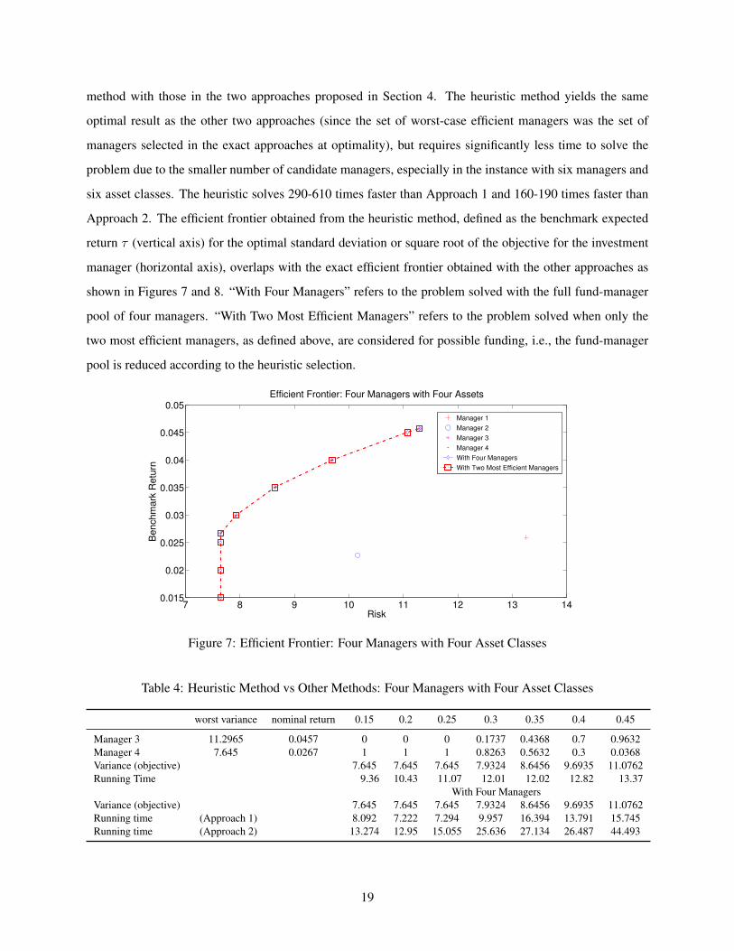
method with those in the two approaches proposed in Section 4. The heuristic method yields the same

optimal result as the other two approaches (since the set of worst-case efficient managers was the set of

managers selected in the exact approaches at optimality), but requires significantly less time to solve the

problem due to the smaller number of candidate managers, especially in the instance with six managers and

six asset classes. The heuristic solves 290-610 times faster than Approach 1 and 160-190 times faster than

Approach 2. The efficient frontier obtained from the heuristic method, defined as the benchmark expected

return τ (vertical axis) for the optimal standard deviation or square root of the objective for the investment

manager (horizontal axis), overlaps with the exact efficient frontier obtained with the other approaches as

shown in Figures 7 and 8. “With Four Managers” refers to the problem solved with the full fund-manager

pool of four managers. “With Two Most Efficient Managers” refers to the problem solved when only the

two most efficient managers, as defined above, are considered for possible funding, i.e., the fund-manager

pool is reduced according to the heuristic selection.

7 8 9 10 11 12 13 140.015

0.02

0.025

0.03

0.035

0.04

0.045

0.05

Risk

Be

nchm

ark

Retu

rn

Efficient Frontier: Four Managers with Four Assets

Manager 1

Manager 2

Manager 3

Manager 4

With Four Managers

With Two Most Efficient Managers

Figure 7: Efficient Frontier: Four Managers with Four Asset Classes

Table 4: Heuristic Method vs Other Methods: Four Managers with Four Asset Classes

worst variance nominal return 0.15 0.2 0.25 0.3 0.35 0.4 0.45

Manager 3 11.2965 0.0457 0 0 0 0.1737 0.4368 0.7 0.9632Manager 4 7.645 0.0267 1 1 1 0.8263 0.5632 0.3 0.0368Variance (objective) 7.645 7.645 7.645 7.9324 8.6456 9.6935 11.0762Running Time 9.36 10.43 11.07 12.01 12.02 12.82 13.37

With Four ManagersVariance (objective) 7.645 7.645 7.645 7.9324 8.6456 9.6935 11.0762Running time (Approach 1) 8.092 7.222 7.294 9.957 16.394 13.791 15.745Running time (Approach 2) 13.274 12.95 15.055 25.636 27.134 26.487 44.493

19

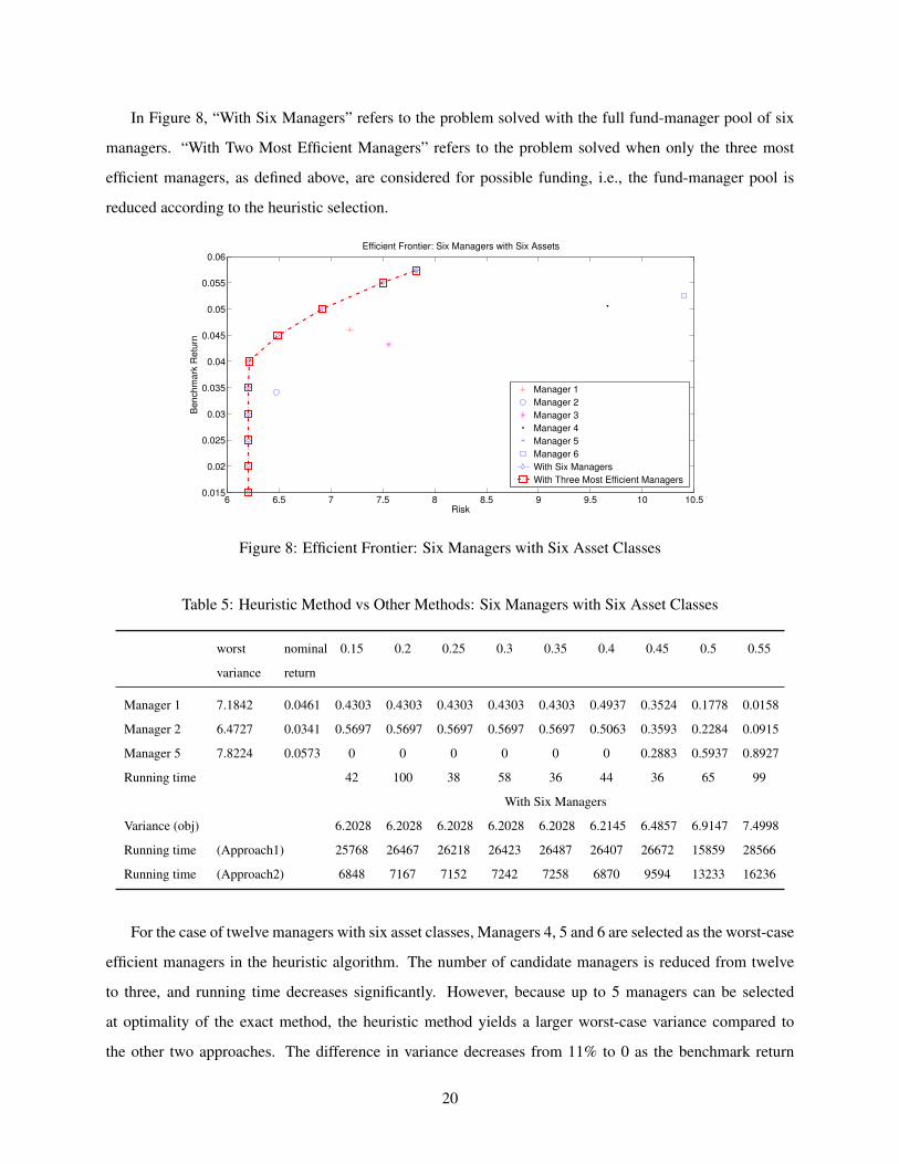
In Figure 8, “With Six Managers” refers to the problem solved with the full fund-manager pool of six

managers. “With Two Most Efficient Managers” refers to the problem solved when only the three most

efficient managers, as defined above, are considered for possible funding, i.e., the fund-manager pool is

reduced according to the heuristic selection.

6 6.5 7 7.5 8 8.5 9 9.5 10 10.50.015

0.02

0.025

0.03

0.035

0.04

0.045

0.05

0.055

0.06

Risk

Be

nch

ma

rk R

etu

rn

Efficient Frontier: Six Managers with Six Assets

Manager 1

Manager 2

Manager 3

Manager 4

Manager 5

Manager 6

With Six Managers

With Three Most Efficient Managers

Figure 8: Efficient Frontier: Six Managers with Six Asset Classes

Table 5: Heuristic Method vs Other Methods: Six Managers with Six Asset Classes

worst

variance

nominal

return

0.15 0.2 0.25 0.3 0.35 0.4 0.45 0.5 0.55

Manager 1 7.1842 0.0461 0.4303 0.4303 0.4303 0.4303 0.4303 0.4937 0.3524 0.1778 0.0158

Manager 2 6.4727 0.0341 0.5697 0.5697 0.5697 0.5697 0.5697 0.5063 0.3593 0.2284 0.0915

Manager 5 7.8224 0.0573 0 0 0 0 0 0 0.2883 0.5937 0.8927

Running time 42 100 38 58 36 44 36 65 99

With Six Managers

Variance (obj) 6.2028 6.2028 6.2028 6.2028 6.2028 6.2145 6.4857 6.9147 7.4998

Running time (Approach1) 25768 26467 26218 26423 26487 26407 26672 15859 28566

Running time (Approach2) 6848 7167 7152 7242 7258 6870 9594 13233 16236

For the case of twelve managers with six asset classes, Managers 4, 5 and 6 are selected as the worst-case

efficient managers in the heuristic algorithm. The number of candidate managers is reduced from twelve

to three, and running time decreases significantly. However, because up to 5 managers can be selected

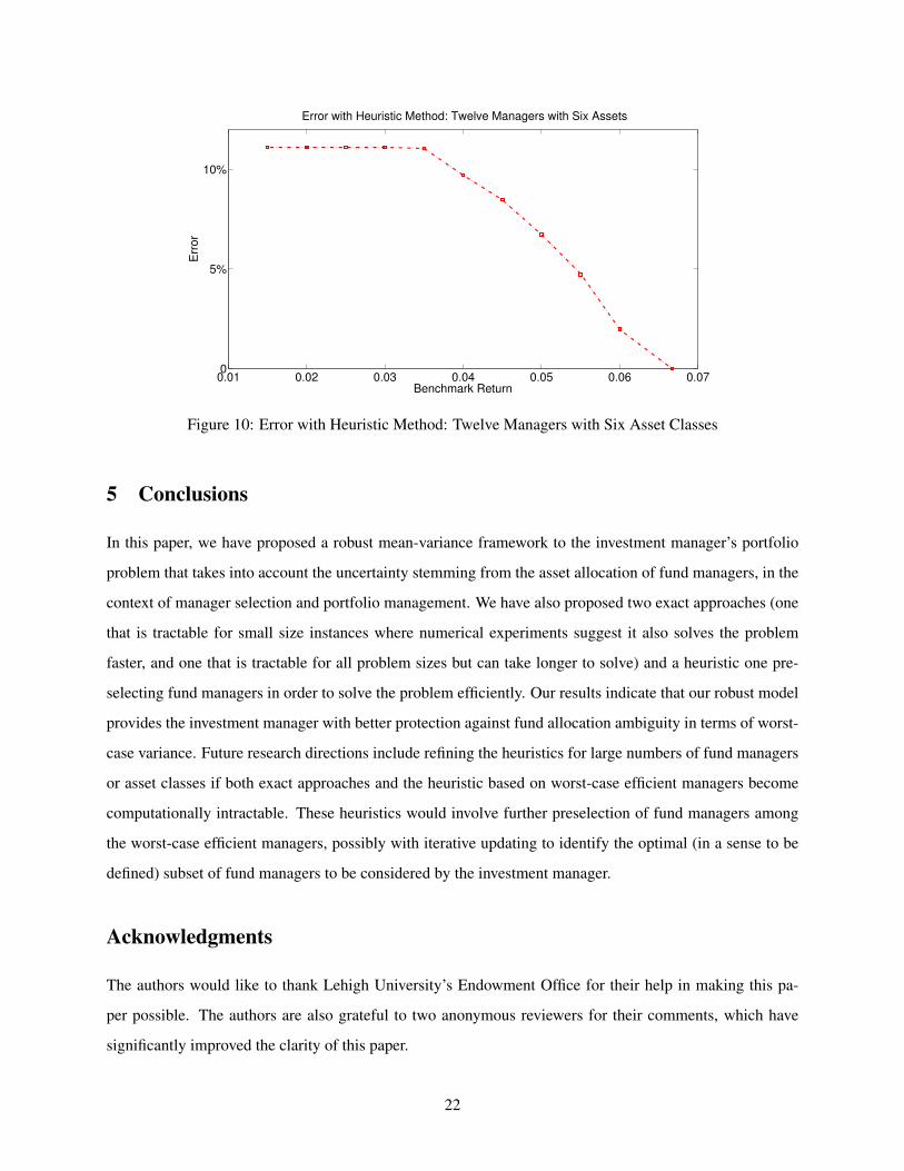
at optimality of the exact method, the heuristic method yields a larger worst-case variance compared to

the other two approaches. The difference in variance decreases from 11% to 0 as the benchmark return

20

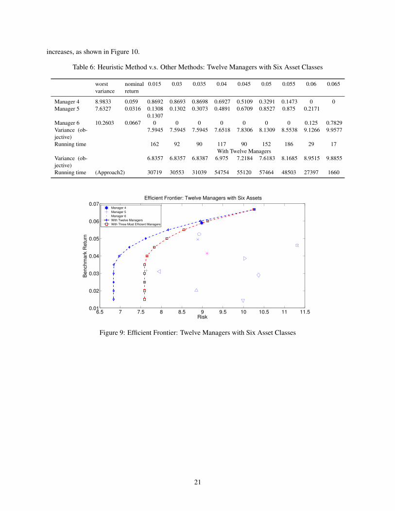
increases, as shown in Figure 10.

Table 6: Heuristic Method v.s. Other Methods: Twelve Managers with Six Asset Classes

worstvariance

nominalreturn

0.015 0.03 0.035 0.04 0.045 0.05 0.055 0.06 0.065

Manager 4 8.9833 0.059 0.8692 0.8693 0.8698 0.6927 0.5109 0.3291 0.1473 0 0Manager 5 7.6327 0.0316 0.1308

0.13070.1302 0.3073 0.4891 0.6709 0.8527 0.875 0.2171

Manager 6 10.2603 0.0667 0 0 0 0 0 0 0 0.125 0.7829Variance (ob-jective)

7.5945 7.5945 7.5945 7.6518 7.8306 8.1309 8.5538 9.1266 9.9577

Running time 162 92 90 117 90 152 186 29 17With Twelve Managers

Variance (ob-jective)

6.8357 6.8357 6.8387 6.975 7.2184 7.6183 8.1685 8.9515 9.8855

Running time (Approach2) 30719 30553 31039 54754 55120 57464 48503 27397 1660

6.5 7 7.5 8 8.5 9 9.5 10 10.5 11 11.50.01

0.02

0.03

0.04

0.05

0.06

0.07

Risk

Benchm

ark

Retu

rn

Efficient Frontier: Twelve Managers with Six Assets

Manager 4

Manager 5

Manager 6

With Twelve Managers

With Three Most Efficient Managers

Figure 9: Efficient Frontier: Twelve Managers with Six Asset Classes

21

0.01 0.02 0.03 0.04 0.05 0.06 0.070

5%

10%

Error with Heuristic Method: Twelve Managers with Six Assets

Benchmark Return

Err

or

Figure 10: Error with Heuristic Method: Twelve Managers with Six Asset Classes

5 Conclusions

In this paper, we have proposed a robust mean-variance framework to the investment manager’s portfolio

problem that takes into account the uncertainty stemming from the asset allocation of fund managers, in the

context of manager selection and portfolio management. We have also proposed two exact approaches (one

that is tractable for small size instances where numerical experiments suggest it also solves the problem

faster, and one that is tractable for all problem sizes but can take longer to solve) and a heuristic one pre-

selecting fund managers in order to solve the problem efficiently. Our results indicate that our robust model

provides the investment manager with better protection against fund allocation ambiguity in terms of worst-

case variance. Future research directions include refining the heuristics for large numbers of fund managers

or asset classes if both exact approaches and the heuristic based on worst-case efficient managers become

computationally intractable. These heuristics would involve further preselection of fund managers among

the worst-case efficient managers, possibly with iterative updating to identify the optimal (in a sense to be

defined) subset of fund managers to be considered by the investment manager.

Acknowledgments

The authors would like to thank Lehigh University’s Endowment Office for their help in making this pa-

per possible. The authors are also grateful to two anonymous reviewers for their comments, which have

significantly improved the clarity of this paper.

22

References

[1] R. Arnott, J. Jsu, and P. Moore. Fundamental indexation. Financial Analysts Journal, 61:83–99, 2005.

[2] C. Barry and L. Starks. Investment management and risk-sharing with multiple managers. Journal of

Finance, 39(2):477–491, 1984.

[3] A. Ben-Tal, T. Margalit, and A. Nemirovski. Robust modeling of multi-stage portfolio problems. High

Performance Optimization, Kluwer Academic Publishers:125–158, 2000.

[4] A. Ben-Tal, L. El-Ghaoui, and A. Nemirovski. Robust optimization. Princeton University Press, 2009.

Princeton, NJ.

[5] J. Benders. Partitioning procedures for solving mixed-variables programming problems. Numer. Math.,

pages 238–252, 1962.

[6] D. Bertsimas, D.B. Brown, and C. Caramanis. Theory and applications of robust optimization. SIAM

Review, 53:464–501, 2011.

[7] D. Bienstock and N. Ozbay. Computing robust basestock levels. Discrete Optimization, 5, 2008.

[8] D. Blake, A. Rossi, A. Timmermann, I. Tonks, and R. Wermers. Decentralized investment manage-

ment: Evidence from the pension fund industry. Journal of Finance, 68(3):1133–1178, 2013.

[9] G. Brinson, R. Hood, and G. Beebower. Determinants of portfolio performance. The Financial Ana-

lysts Journal, pages 39–44, 1986.

[10] J. Chen and S. Burer. Globally solving nonconvex quadratic programming problems via completely

positive programming. Mathematical Programming Computations, 4:33–52, 2012.

[11] V. Chopra and W. Ziemba. The effect of errors in means, variances and covariances on optimal portfolio

choice. In W. Ziemba and J. Mulvey, editors, Worldwide asset and liability modeling. Cambridge

University Press, 1998.

[12] E. Delage and Y. Ye. Distributionally robust optimization under moment uncertainty with application

to data-driven problems. Operations Research, 58(3):595–612, 2010.

[13] V. DeMiguel and F. Nogales. Portfolio selection with robust estimation. Operations Research, 57(3):

560–577, 2009.

23

[14] V. DeMiguel, A. Martin-Utrera, and F. Nogales. Size matters: Optimal calibration of shrinkage esti-

mators for portfolio selection. Journal of Banking and Finance, 37(8):3018–3034, 2013.

[15] L. El-Ghaoui, M. Oks, and F Oustry. Worst-case value-at-risk and robust portfolio optimization: a

conic programming approach. Operations Research, 51(4):543–556, 2003.

[16] E. Elton and M. Gruber. Optimum centralized portfolio construction with decentralized portfolio

management. Financial and Quantitative Analysis, 39(3):481–494, 2004.

[17] L. Garlappi, R. Uppal, and T. Wang. Portfolio selection with parameter and model uncertainty: A

multi-prior approach. Review of Financial Studies, 20(1):41–81, 2007.

[18] D. Goldfarb and G.N. Iyengar. Robust portfolio selection problems. Mathematics of Operations

Research, 28:1–38, 2003.

[19] M. Grinblatt and S. Titman. Performance measurement without benchmarks: An examination of

mutual fund returns. Journal of Business, 66:47–68, 1993.

[20] C. Hsu and W. Myers. Performance attribution: Measuring dynamic allocation skill. Financial Analysts

Journal, 66(6), 2010.

[21] M. Jensen. The performance of mutual funds in the period 1945-1964. Journal of Finance, 23:389–

416, 1968.

[22] M. Jensen. Risk, the pricing of capital assets, and the evaluation of investment performance. Journal

of Business, 42:167–247, 1969.

[23] O. Ledoit and M. Wolf. Honey, I shrunk the sample covariance matrix. Journal of Portfolio Manage-

ment, 30(4):110–119, 2004.

[24] W. Lo. Where do alphas come from?: A measure of the value of active investment management.

Journal of Investment Management, 6(22), 2008.

[25] J. Maginn, D. Tuttle, D. McLeavey, and J. Pinto, editors. Managing Investment Portfolios: A Dynamic

Process. Wiley, 2007.

[26] S. Maillard, T. Roncalli, and J. Teiletche. The properties of equally weighted risk contribution portfo-

lios. Journal of Portfolio Management, 36(4):60–70, 2010.

[27] H. Markowitz. Portfolio selection. The Journal of Finance, 7(1):77–91, 1952.

24

[28] G. Pflug and D. Wozabal. Ambiguity in portfolio selection. Quantitative Finance, 7(4):435–442, 2007.

[29] A. Reed, C. Tiu, and U. Yoeli. Decentralized downside risk management. Journal of Investment

Management, 9(1):72–98, 2011.

[30] T. Roncalli. Introduction to Risk Parity and Budgeting. Chapman&Hall/CRC Financial Mathematics

Series, 2013.

[31] W. Sharpe. Mutual fund performance. Journal of Business, 39:119–138, 1966.

[32] W. Sharpe. Decentralized investment management. Journal of Finance, 36(2):217–234, 1981.

[33] H.D. Sherali and W.P. Adams. A Reformulation-Linearization Technique for Solving Discrete and

Continuous Nonconvex Problems. Kluwer, Dordrecht, 1998.

[34] D. Swensen. Pioneering portfolio management: an unconventional approach to institutional invest-

ment, fully revised and updated. Free Press, 2009.

[35] A. Thiele, T. Terry, and M. Epelman. Robust linear optimization with recourse. Technical report,

Lehigh University, 2010.

[36] J. Treynor. How to rate management of investment funds. Harvard Business Review, 43:63–75, 1965.

[37] J. Treynor. Why market-valuation-indifferent indexing works. Financial Analysts Journal, 61:65–69,

2005.

[38] J. Treynor and K. Mazuy. Can mutual funds outguess the market? Harvard Business Review, 44:

131–163, 1966.

[39] H. Tuy. Concave Minimization under Linear Constraints with Special Structure. Hanoi:Hanoi Inst.

Math, 1983.

[40] J. Van Binsbergen, M. Brandt, and R. Koijen. Optimal decentralized investment management. Journal

of Finance, 63(4):1849–1894, 2008.

[41] B. Zeng. Solving two-stage robust optimization problems by a constraint-and-column generation

method. Technical report, University of South Florida, 2011.

[42] L. Zhang. Multi-period pricing for perishable products: Uncertainty and competition. Master’s thesis,

M.I.T., 2006.

25