Embed Size (px)
Citation preview
Robust Model PredictiveControl
Colloquium on Predictive Control
University of Sheffield, April 4, 2005
David Mayne
(with Maria Seron and Sasa Rakovic)
Imperial College London
IC – p.1/25
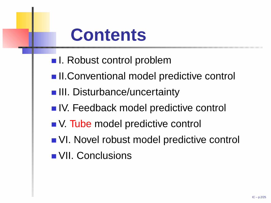
ContentsI. Robust control problem
II.Conventional model predictive control
III. Disturbance/uncertainty
IV. Feedback model predictive control
V. Tube model predictive control
VI. Novel robust model predictive control
VII. Conclusions
IC – p.2/25
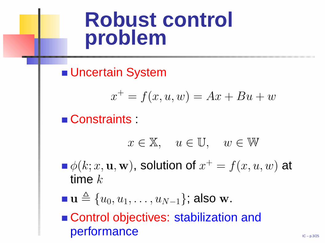
Robust controlproblem
Uncertain System
x+ = f(x, u, w) = Ax + Bu + w
Constraints :
x ∈ X, u ∈ U, w ∈ W
φ(k; x,u,w), solution of x+ = f(x, u, w) attime k
u , {u0, u1, . . . , uN−1}; also w.
Control objectives: stabilization andperformance IC – p.3/25
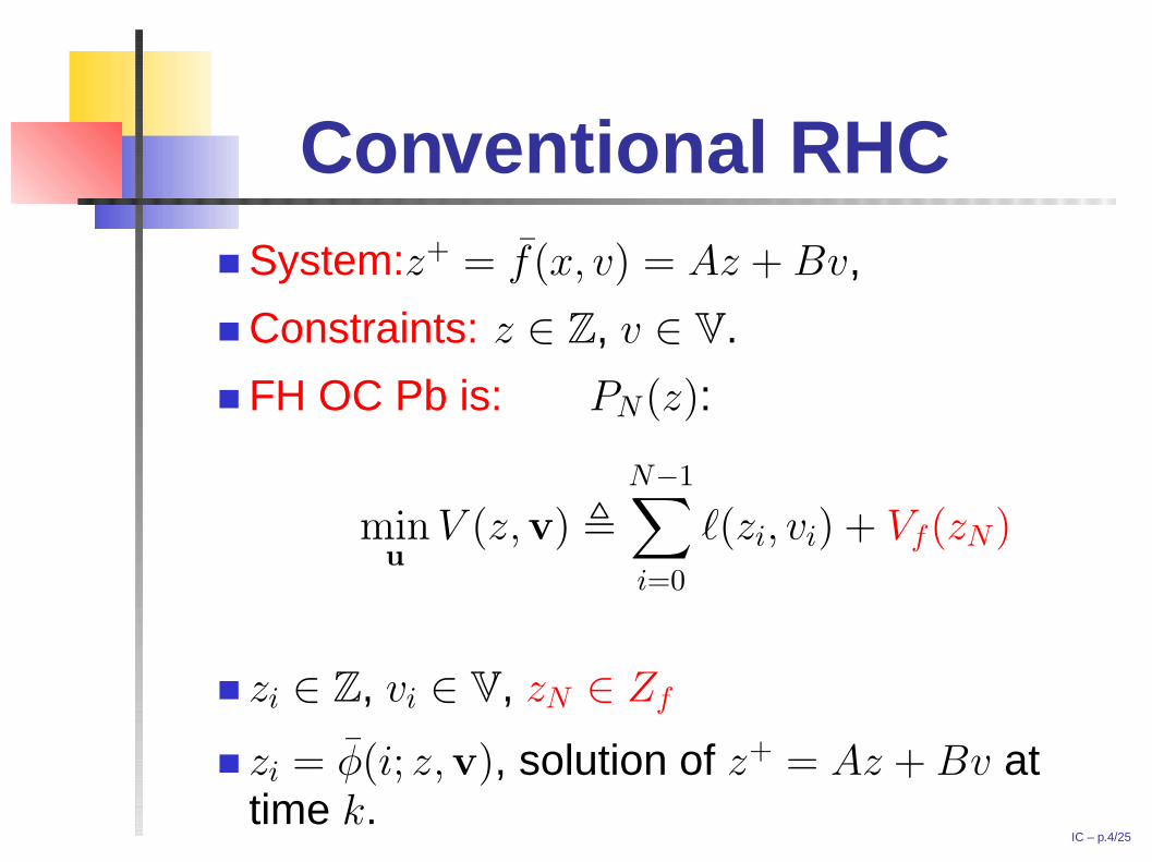
Conventional RHCSystem:z+ = f(x, v) = Az + Bv,
Constraints: z ∈ Z, v ∈ V.
FH OC Pb is: PN (z):
minu
V (z,v) ,
N−1∑
i=0
`(zi, vi) + Vf(zN)
zi ∈ Z, vi ∈ V, zN ∈ Zf
zi = φ(i; z,v), solution of z+ = Az + Bv attime k.
IC – p.4/25
Conventional RHCSolution: v
0(z) = {v00(z), v0
1(z), . . . , v0N−1
(z)}.
Value f’n: V 0N(z) = VN(z,v0(z)), domain ZN .
RH control law: κN(z) , v0(0; z).
IF A: Vf(·) is local CLF in sense:
minv∈V{Vf(f(z, u)) + `(z, u) | f(z, u) ∈Zf} ≤ Vf(z) for all z ∈ Zf ,THEN:
V 0N(f(z, κN (z)) + `(z, κN (z)) ≤ V 0
N(z) ∀z ∈ ZN
and V 0N(z) ≤ Vf(z) ∀z ∈ Zf =⇒ V 0
N(·) is aLyapunov fn for controlled system.
IC – p.5/25
Value function V 0N(·)
Proposition 1 Assume that `(·) and Vf(·) arequadratic and pos. def. and that (stabilizing)assumption A is satisfied. Then
V 0
N(z) ≥ c1|z|2, ∀z ∈ ZN
V 0
N(f(z, κN (z)) ≤ V 0
N(z) − c1|z|2, ∀z ∈ ZN
V 0
N(z) ≤ c2|z|2, ∀z ∈ Zf
Theorem 1 The origin is exp.stable for nominalsystem with MPC law κN(·) (if ZN is bounded).Solution same as that obtained with DP. IC – p.6/25
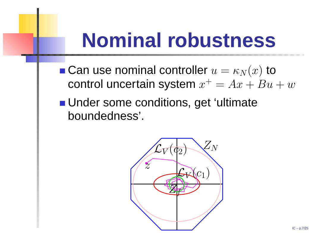
Nominal robustnessCan use nominal controller u = κN(x) tocontrol uncertain system x+ = Ax + Bu + w
Under some conditions, get ‘ultimateboundedness’.
PSfrag replacements
Zf
z
ZNLV (c2)
LV (c1)
IC – p.7/25
‘Feedback’ RHCConservative. State constraints may renderx+ = f(x, κN (x)) non-robust (Teel)
better to design controller to be robust.
predicting effect of uncertainty
hence, use feedback RHC (in which decisionvariable is policy π = {µ0(·), µ1(·), . . . , µN−1(·)}(sequence of control laws).
rather than u = {u0, u1, . . . , uN−1} (sequenceof control actions ).
IC – p.8/25
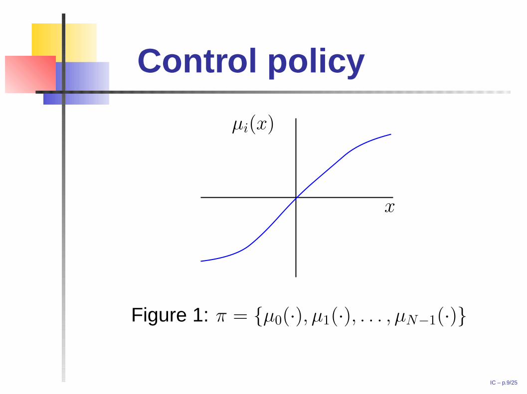
Control policy
PSfrag replacements
µi(x)
x
Figure 1: π = {µ0(·), µ1(·), . . . , µN−1(·)}
IC – p.9/25
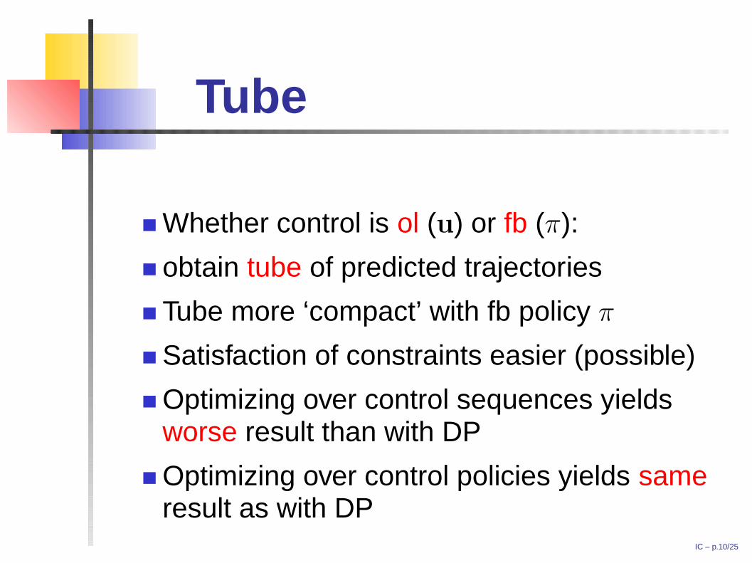
Tube
Whether control is ol (u) or fb (π):
obtain tube of predicted trajectories
Tube more ‘compact’ with fb policy π
Satisfaction of constraints easier (possible)
Optimizing over control sequences yieldsworse result than with DP
Optimizing over control policies yields sameresult as with DP
IC – p.10/25
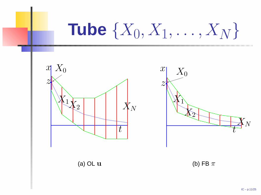
Tube {X0, X1, . . . , XN}
PSfrag replacements
z
x
t
X0
X1X2 XN
(a) OL u
PSfrag replacements
z
x
t
X0
X1
X2
XN
(b) FB π
IC – p.11/25
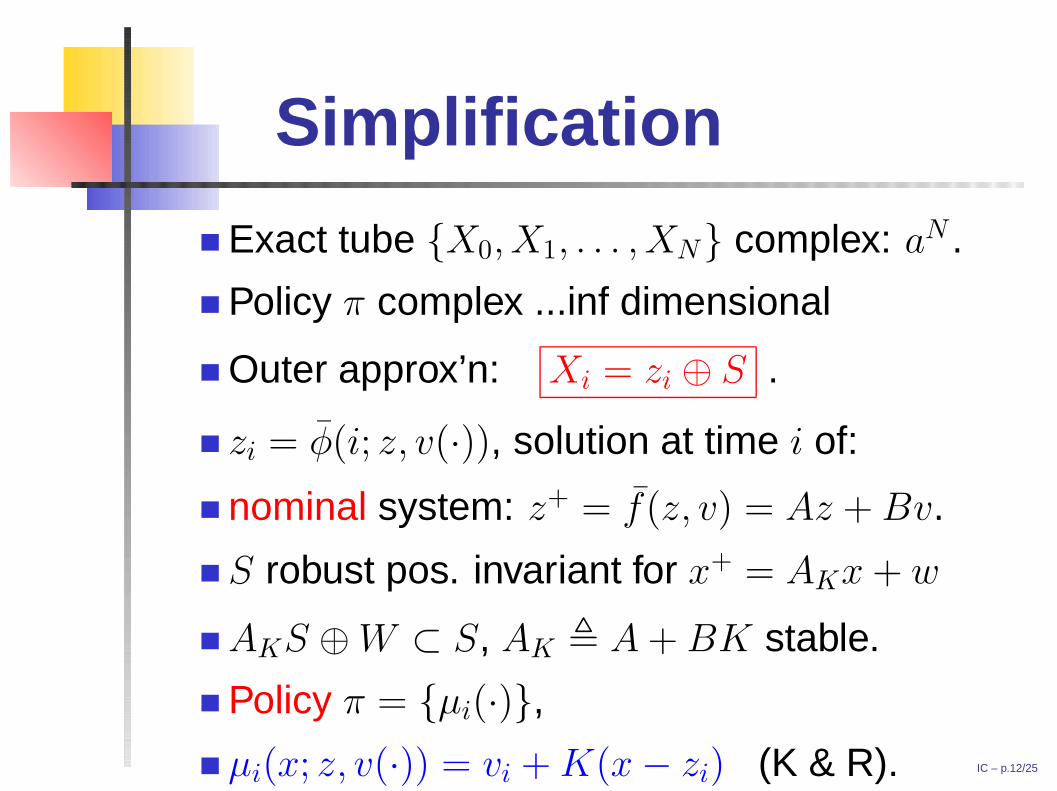
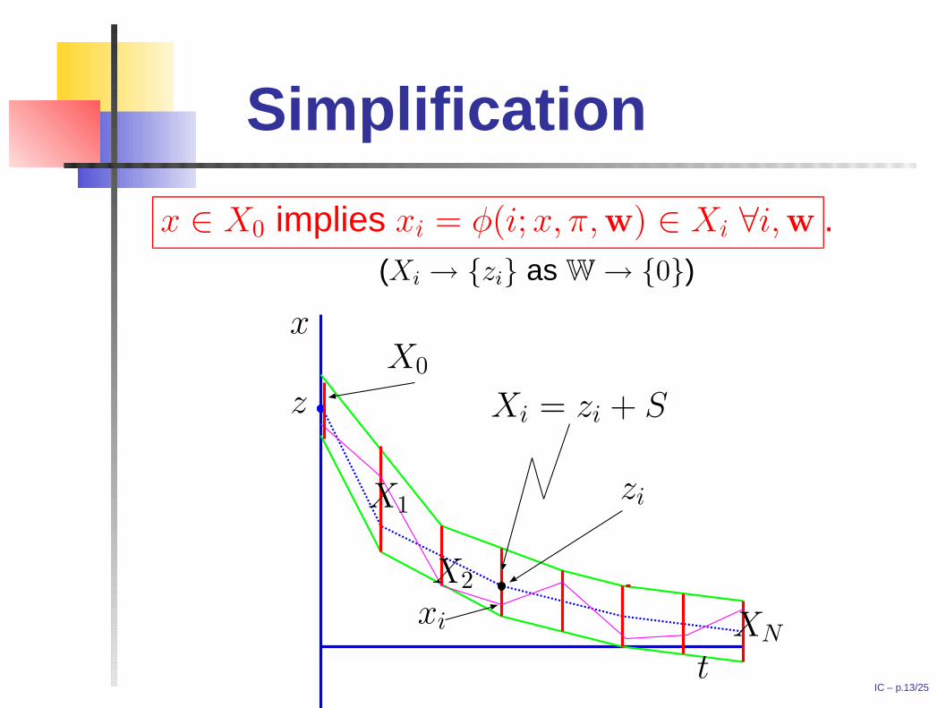
Simplification
Exact tube {X0, X1, . . . , XN} complex: aN .
Policy π complex ...inf dimensional
Outer approx’n: Xi = zi ⊕ S .
zi = φ(i; z, v(·)), solution at time i of:
nominal system: z+ = f(z, v) = Az + Bv.
S robust pos. invariant for x+ = AKx + w
AKS ⊕ W ⊂ S, AK , A + BK stable.
Policy π = {µi(·)},
µi(x; z, v(·)) = vi + K(x − zi) (K & R). IC – p.12/25
Simplification
x ∈ X0 implies xi = φ(i; x, π,w) ∈ Xi ∀i,w .(Xi → {zi} as W → {0})
PSfrag replacements
z
x
t
X0
X1
X2
XNxi
zi
Xi = zi + S
Figure 2: Tube
IC – p.13/25
Nominal OC PbNominal system is z+ = Az + Bv.
φ(i; z,v) is sol’n at i of nominal system.
Nominal OC Pb: same as before with tighterconstraints:
vi ∈ V , U KS (W small enough)
zi ∈ Z , X S (W small enough)
zN ∈ Zf ⊂ X S, where
UN(z) = {v satisfying all constraints , z(0) = z}
(C&R&Z, M&L)
IC – p.14/25
Control policy
Consider policy π0 = π0(z) constructed fromsolution to modified nominal OC Pb:
π0(z) , {µ0(·; z), µ1(·; z), . . . , µN−1(·; z)}
µi(x; z) , v0i (z) + K(x − z0
i (z))
Proposition 2 Policy π0(z) steers any any initialstate of x+ = Ax + Bu + w lying in X0(x) = z ⊕ Sto Xf = Zf ⊕ S ⊆ X in N steps satisfying allconstraints for all admissible disturbancesequences. (C&R&Z, M&L)
IC – p.15/25
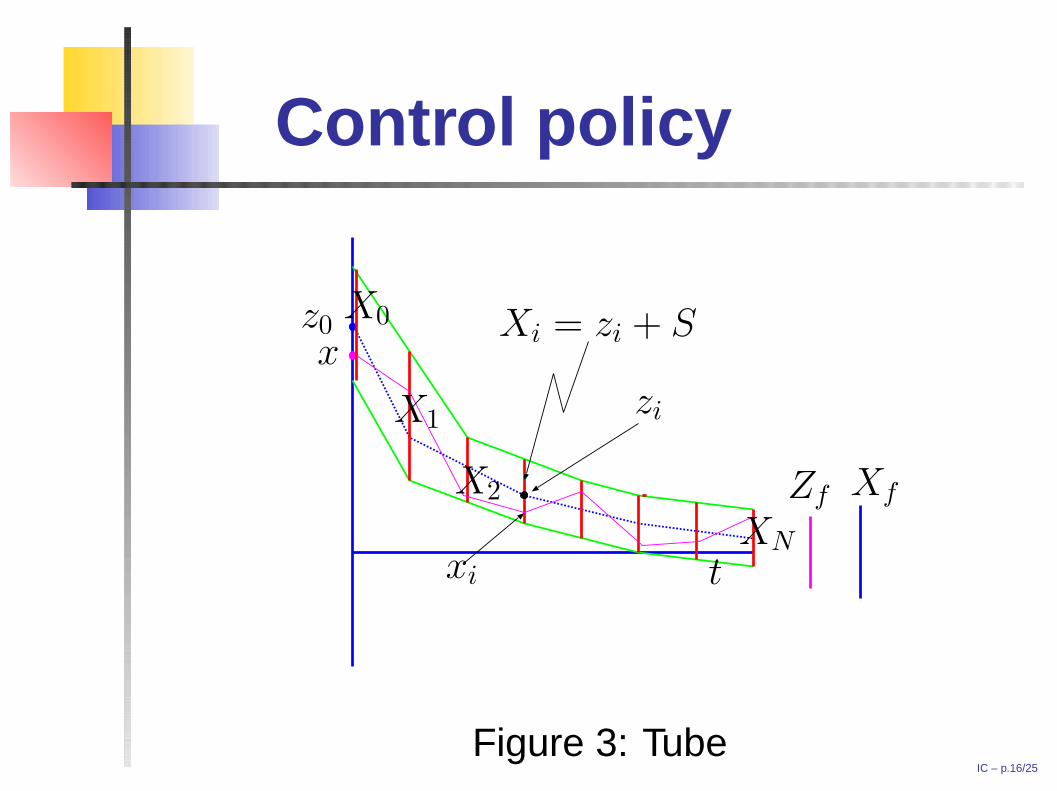
Control policyPSfrag replacements
xz0
t
X0
X1
X2
XNxi
zi
Xi = zi + S
Zf Xf
Figure 3: TubeIC – p.16/25
Receding horizon
Above ... single shot
Receding horizon ... two factors:
Controlling tube ...not a trajectory
Control to set S (not origin) ... S is robust‘origin’
Prob. 1: Assumption equivalent to A for casewhen terminal ‘state’ is a set X rather than apoint x?
Prob. 2: Value function that is zero in S (theorigin)?
IC – p.17/25
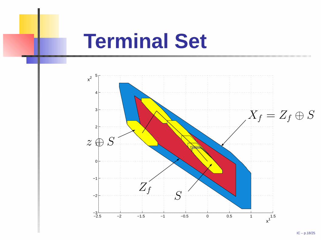
Terminal Set
−2.5 −2 −1.5 −1 −0.5 0 0.5 1 1.5−3
−2
−1
0
1
2
3
4
5
x1
x2
PSfrag replacements
Xf = Zf ⊕ S
Zf
z ⊕ S
S
IC – p.18/25
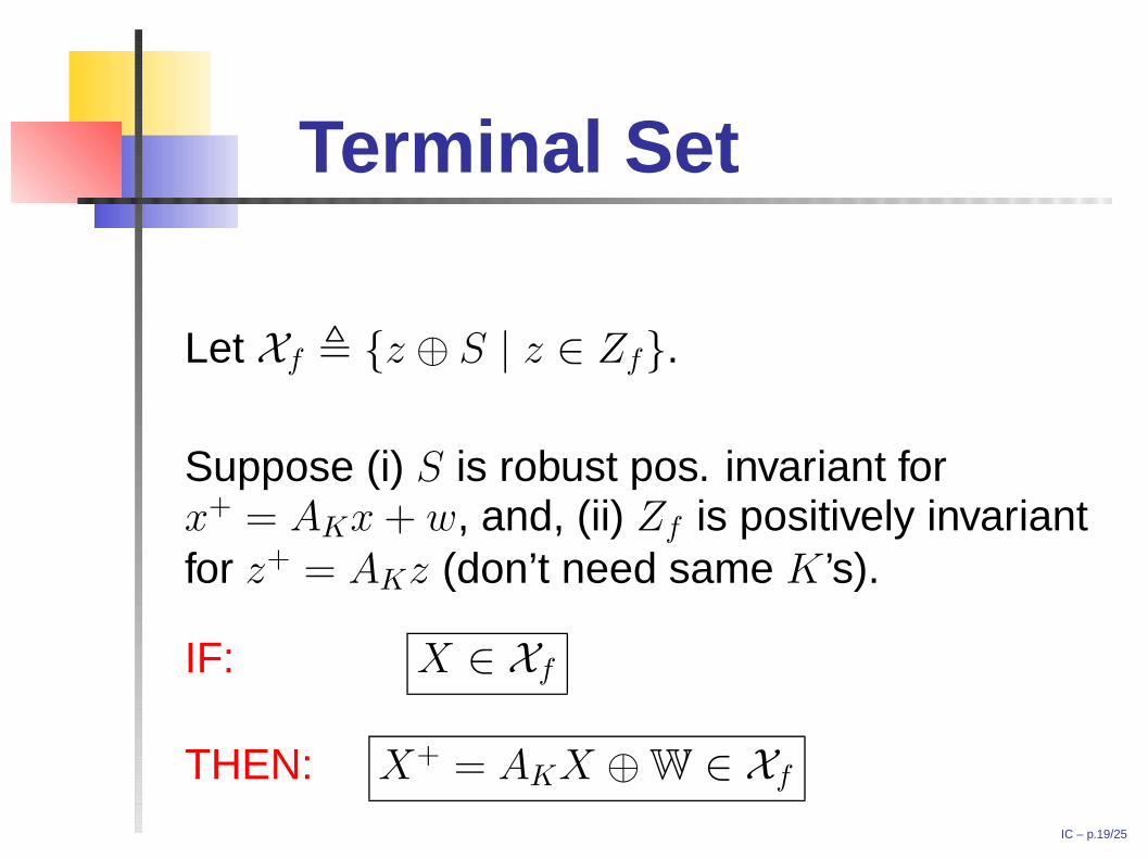
Terminal Set
Let Xf , {z ⊕ S | z ∈ Zf}.
Suppose (i) S is robust pos. invariant forx+ = AKx + w, and, (ii) Zf is positively invariantfor z+ = AKz (don’t need same K ’s).
IF: X ∈ Xf
THEN: X+ = AKX ⊕ W ∈ Xf
IC – p.19/25
New Optimal ControlProblem
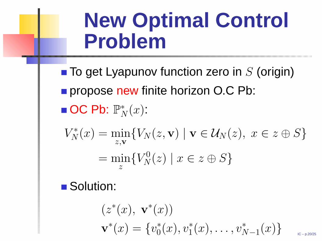
To get Lyapunov function zero in S (origin)
propose new finite horizon O.C Pb:
OC Pb: P∗N(x):
V ∗N(x) = min
z,v{VN(z,v) | v ∈ UN(z), x ∈ z ⊕ S}
= minz{V 0
N(z) | x ∈ z ⊕ S}
Solution:
(z∗(x), v∗(x))
v∗(x) = {v∗0(x), v∗1(x), . . . , v∗N−1(x)}
IC – p.20/25

Model predictivecontrol law
Implicit model predictive control law:
κ∗N(x) = v∗0(x) + K(x − z∗(x))
PSfrag replacementsz∗(x)
x ⊕ S
x
IC – p.21/25
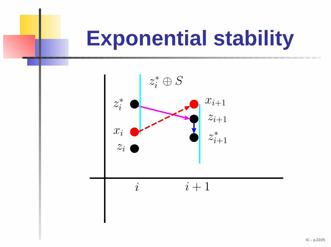
Exponential stability
PSfrag replacementsz∗i
zi+1
z∗i+1
xi
xi+1
z∗i ⊕ S
zi
i i + 1
IC – p.22/25
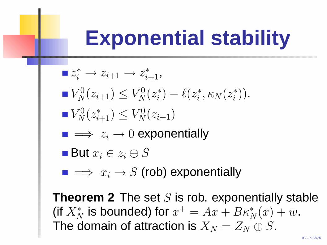
Exponential stabilityz∗i → zi+1 → z∗i+1,
V 0N(zi+1) ≤ V 0
N(z∗i ) − `(z∗i , κN(z∗i )).
V 0N(z∗i+1) ≤ V 0
N(zi+1)
=⇒ zi → 0 exponentially
But xi ∈ zi ⊕ S
=⇒ xi → S (rob) exponentially
Theorem 2 The set S is rob. exponentially stable(if X∗
N is bounded) for x+ = Ax + Bκ∗N(x) + w.
The domain of attraction is XN = ZN ⊕ S.IC – p.23/25
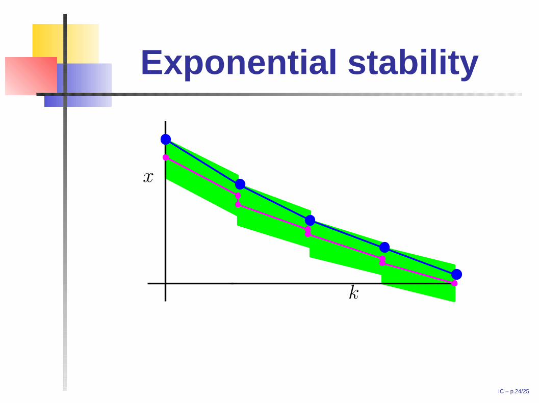
Exponential stability
PSfrag replacements
x
k
IC – p.24/25
ConclusionsHave presented novel version of modelpredictive control
Uses feedback mpc and bounding tube
And initial state as a decision variable
Simple online optimization problem (QP)
V ∗N(·) zero in set S (origin)
Set S is exponentially stable
Moral : control tube, not individualtrajectories.
IC – p.25/25


![Yasir K. Al-Nadawi, Hothaifa Al-Qassab, Daniel Kent, Su ...control methodologies such as linear model predictive control (MPC) [4,5], nonlinear robust model predictive control (NRMPC)](https://img.pdfslide.net/doc/110x75/603cfecc7ab1ef60065e6de3/yasir-k-al-nadawi-hothaifa-al-qassab-daniel-kent-su-control-methodologies.jpg)


![Robust Model Predictive Control - Carnegie Mellon …cepac.cheme.cmu.edu/.../Ronust_Control_Classnotes.pdf1 Robust Model Predictive Control Formulations of robust control [1] The robust](https://img.pdfslide.net/doc/110x75/5aab45707f8b9a2b4c8bd345/robust-model-predictive-control-carnegie-mellon-cepacchemecmueduronustcontrol.jpg)