Robust Network Compressive Sensing

Yi-Chao ChenThe University of Texas at Austin

Joint work withLili Qiu*, Yin Zhang*, Guangtao Xue+, Zhenxian

Hu+

The University of Texas at Austin*

Shanghai Jiao Tong University+

ACM MobiCom 2014September 10, 2014

Network Matrices and Applications

• Network matrices– Traffic matrix– Loss matrix– Delay matrix– Channel State Information (CSI) matrix– RSS matrix

2

3

Q: How to fill in missing values in a matrix?

1

3

2router

flow 1

flow 3

flow 2

link 2link 1

link 3

flow 1

flow 2

flow 3

time 1 time 2 …

• Applications need complete network matrices– Traffic engineering– Spectrum sensing– Channel estimation– Localization– Multi-access channel design– Network coding, wireless video coding– Anomaly detection– Data aggregation– …

Missing Values: Why Bother?4

subcarrier 1

subcarrier 2

subcarrier 3

time 1 time 2 …

Vacant

freq 1

freq 2

freq 3

time 1 time 2 …

5

The Problem

6,3

6,2

6,1

5,3

5,2

5,1

4,13,32,3

4,13,22,2

4,13,12,1

1,3

1,2

1,1

x

x

x

x

x

x

xxx

xxx

xxx

x

x

x

X

Interpolation: fill in missing values from incomplete, erroneous, and/or indirect measurements

Anomaly FutureMissing

x1,3

6

State of the Art• Exploit low-rank nature of network

matrices– matrices are low-rank [LPCD+04, LCD04,

SIGCOMM09]:

Xnxm Lnxr * RmxrT (r « n,m)

• Exploit spatio-temporal properties– matrix rows or columns close to each other

are often close in value [SIGCOMM09]

• Exploit local structures in network matrices– matrices have both global & local structures– Apply K-Nearest Neighbor (KNN) for local

interpolation [SIGCOMM09]

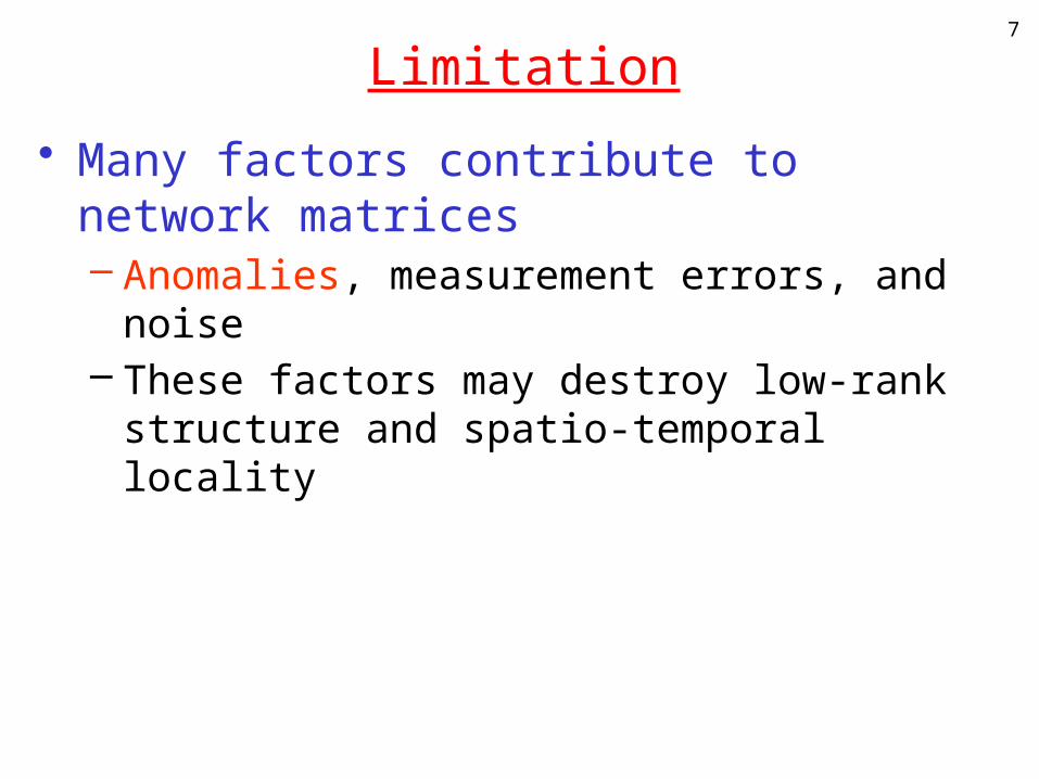
Limitation

• Many factors contribute to network matrices– Anomalies, measurement errors, and noise– These factors may destroy low-rank

structure and spatio-temporal locality

7

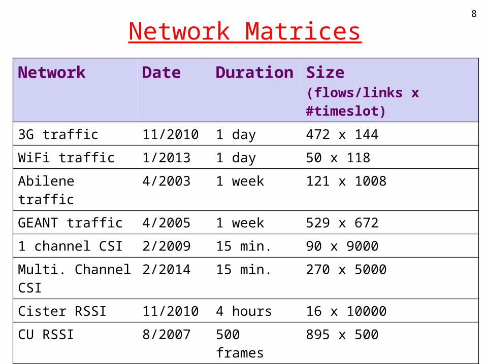
Network Matrices

Network Date Duration Size (flows/links x #timeslot)

3G traffic 11/2010 1 day 472 x 144

WiFi traffic 1/2013 1 day 50 x 118

Abilene traffic 4/2003 1 week 121 x 1008

GEANT traffic 4/2005 1 week 529 x 672

1 channel CSI 2/2009 15 min. 90 x 9000

Multi. Channel CSI

2/2014 15 min. 270 x 5000

Cister RSSI 11/2010 4 hours 16 x 10000

CU RSSI 8/2007 500 frames 895 x 500

Umich RSS 4/2006 30 min. 182 x 3127

UCSB Meshnet 4/2006 3 days 425 x 1527

8

Rank Analysis9

GÉANT: 81%UMich RSS: 74%

3G: 32%Cister RSSI: 20%

Not all matrices are low rank.

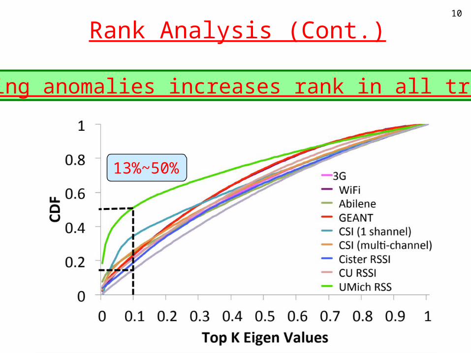
Rank Analysis (Cont.)10

Adding anomalies increases rank in all traces

13%~50%

Temporal Stability11

Temporal stability varies across traces.

3G: 10%Cister RSSI: 6%

UCSB Meshnet: 0.3%UMich RSS: 0.8%

CD

F

Summary of the Analyses

• Our analyses reveal– Real network matrices may not be low rank– Adding anomalies increases the rank– Temporal stability varies across traces

12

Challenges

• How to explicitly account for anomalies, errors, and noise ?

• How to support matrices with different temporal stability?

13

Robust Compressive Sensing

• A new matrix decomposition that is general and robust against error/anomalies– Low rank matrix, anomaly matrix, noise

matrix

• A self-learning algorithm to automatically tune the parameters – Account for varying temporal stability

• An efficient optimization algorithm– Search for the best parameters– Work for large network matrices

14

LENS Decomposition: Basic Formulation

15

= +

y1,30…

…

…y3,n

0 0 0000 00000 0

000 0 0

+

[Input] D:Original matrix

[Output] X:A low rank matrix (r «

m,n)

[Output] Y:A sparse anomaly

matrix

[Output] Z:A small noise

matrix

d1,3d1,2

…

…

…

d2,n

dm,n

d3,n

d1,4 d1,n

d2,1 d2,2 d2,3

d3,1 d3,2 d3,4

dm,2 dm,3 dm,4

…

xm,r

xr,n

…

x1,1

x2,1

x3,1

xm,1

x3,r

x2,r

x1,r

x1,1

xr,1 xr,2

x1,2

xr,3

x1,3 x1,n… …

…

…

…

LENS Decomposition: Basic Formulation

• Formulate it as a convex opt. problem:

16

min:

subject to:

= + +d1,3

d1,2 d1,4

[Input] D:Original matrix

x1,2 x1,4

[Output] X:A low rank

matrix

0 0 y1,3 0

0 0 0 0

0 0 0 0

[Output] Y:A sparse anomaly matrix

[Output] Z:A small noise

matrix

α βσ

LENS Decomposition: Support Indirect Measurement

• The matrix of interest may not be directly observable (e.g., traffic matrices)– AX + BY + CZ + W = D

• A: routing matrix• B: an over-complete anomaly profile matrix• C: noise profile matrix

17

,t,t,t xxy 321 1

3

2router

flow 1

flow 3

flow 2

link 2link 1

link 3

LENS Decomposition: Account for Domain Knowledge

• Domain Knowledge– Temporal stability– Spatial locality– Initial solution

18

min:

subject to:

Optimization Algorithm

• One of many challenges in optimization:– X and Y appear in multiple places in the objective

and constraints– Coupling makes optimization hard

• Reformulation for optimization by introducing auxiliary variables

•

19

min:

subject to:

Optimization Algorithm• Alternating Direction Method (ADM)

– For each iteration, alternate among the optimization of the augmented Lagrangian function by varying each one of X, Xk, Y, Y0, Z, W, M, Mk, N while fixing the other variables

– Improve efficiency through approximate SVD

20

Setting Parameters

• • •

where (mX,nX) is the size of X, (mY,nY) is the size of Y, η(D) is the fraction of entriesneither missing or erroneous, θ is a control parameter that limitscontamination of dense measurement noise

21

min:α βσ σ

Setting Parameters (Cont.)

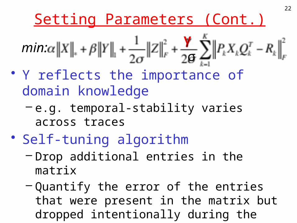
• ϒ reflects the importance of domain knowledge– e.g. temporal-stability varies across traces

• Self-tuning algorithm– Drop additional entries in the matrix– Quantify the error of the entries that were

present in the matrix but dropped intentionally during the search

– Pick ϒ that gives lowest error

22

min:σ

γ

Evaluation Methodology

• Metric– Normalized Mean Absolute Error for missing values

• Report the average of 10 random runs• Anomaly generation

– Inject anomalies to a varying fraction of entries with varying sizes

• Different dropping models

23

24

Algorithms Compared

Algorithm Description

Baseline Baseline estimate via rank-2 approximation

SVD-base SRSVD with baseline removal

SVD-base +KNN Apply KNN after SVD-base

SRMF [SIGCOMM09] Sparsity Regularized Matrix Factorization

SRMF+KNN [SIGCOMM09]

Hybrid of SRMF and KNN

LENS Robust network compressive sensing

Self Learned ϒ25

Best ϒ = 0 Best ϒ = 1 Best ϒ = 10

No single ϒ works for all traces.Self tuning allows us to automatically select the best ϒ.

Interpolation under anomalies26

CU RSSI

LENS performs the best under anomalies.

Interpolation without anomalies27

CU RSSI

LENS performs the best even without anomalies.

Computation Time28

LENS is efficient due to local optimization in ADM.

Summary of Other Results

• The improvement of LENS increases with anomaly sizes and # anomalies.

• LENS consistently performs the best under different dropping modes.

• LENS yields the lowest prediction error.

• LENS achieves higher anomaly detection accuracy.

29

Conclusion

• Main contributions– Important impact of anomalies in matrix

interpolation– Decompose a matrix into

• a low-rank matrix, • a sparse anomaly matrix, • a dense but small noise matrix

– An efficient optimization algorithm– A self-learning algorithm to automatically tune the

parameters• Future work

– Applying it to spectrum sensing, channel estimation, localization, etc.

30

31

Thank you!

BACKUP SLIDES

32

y1,t = x1,t + x2,t

33

Missing Values: Why Bother?

• Missing values are common in network matrices– Measurement and data collection are unreliable– Anomalies/outliers hide non-anomaly-related traffic– Future entries has not yet appeared– Direct measurement is infeasible/expensive

xf,t : traffic of flow f at time t

Missing

x2,4

Anomaly Future

? ? ?

?

?

3

2

1flow 1

flow 2flow 3

Anomaly Generation

• Anomalies in real-world network matrices– The ground truth is hard to get– Injecting the same size of anomalies for all

network matrices is not practical

• Generating anomalies based on the nature of the network matrix [SIGCOMM04, INFOCOM07, PETS11]

– Apply Exponential Weighted Moving Average (EWMA) to predict the matrix

– Calculate the difference between the real matrix and the predicted matrix• The difference is due to prediction error or anomalies

– Sort the difference and select the largest one as the size of anomalies

34

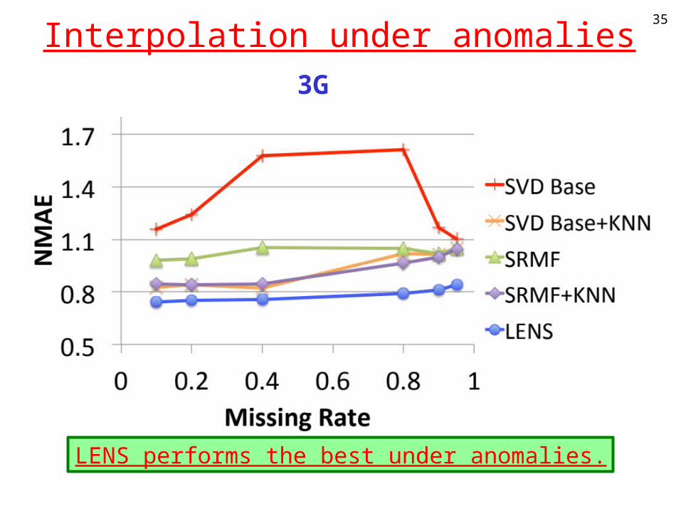
Interpolation under anomalies35

3G

LENS performs the best under anomalies.

Interpolation without anomalies36

3G

LENS performs the best even without anomalies.

Non-monotonicity of Performance

• SVD base method is more sensitive the anomalies

• performance is affected by both the missing rate and the number of anomalies.– As the missing rate increases, the number

of anomalies reduces.• When the missing rate increase, error increases• When the anomalies reduces, error reduces

37

Dropping Models

• Pure Random Loss– Elements are dropped independently with a

random loss rate

38

d1,2

…

… …

d2,n

dm,n

d1,4 d1,n

d2,1 d2,2 d2,3

d3,1 d3,2 d3,4

dm,2 dm,3 dm,4

d1,1 d1,3

d2,4

d3,3 d3,n

dm,1

Dropping Models

• Time Rand Loss– Columns are dropped – To emulate random losses during certain

times• e.g. disk becomes full

39

d1,2

…

… …

d2,n

dm,n

d1,4 d1,n

d2,1 d2,2 d2,3

d3,1 d3,2 d3,4

dm,2 dm,3 dm,4

d1,1 d1,3

d2,4

d3,3 d3,n

dm,1

Dropping Models

• Element Rand Loss– Rows are dropped– To emulate certain nodes lose data

• e.g., due to battery drain

40

d1,2

…

… …

d2,n

dm,n

d1,4 d1,n

d2,1 d2,2 d2,3

d3,1 d3,2 d3,4

dm,2 dm,3 dm,4

d1,1 d1,3

d2,4

d3,3 d3,n

dm,1

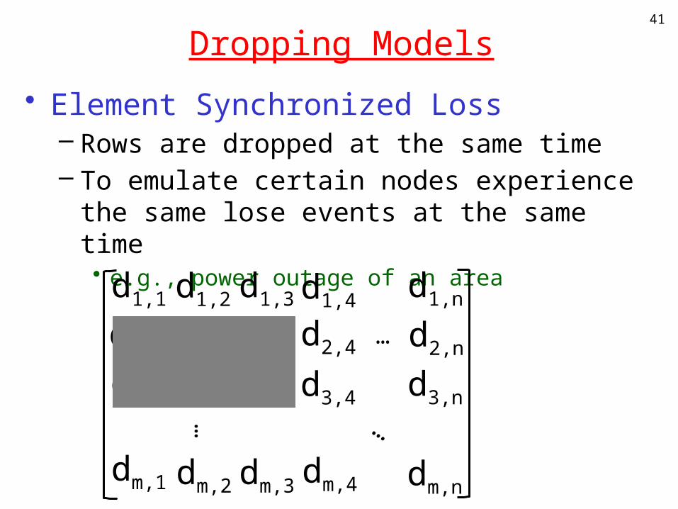
Dropping Models

• Element Synchronized Loss– Rows are dropped at the same time– To emulate certain nodes experience the

same lose events at the same time • e.g., power outage of an area

41

d1,2

…

… …

d2,n

dm,n

d1,4 d1,n

d2,1 d2,2 d2,3

d3,1 d3,2 d3,4

dm,2 dm,3 dm,4

d1,1 d1,3

d2,4

d3,3 d3,n

dm,1

Impact of Dropping models42

LENS consistently performs the best under different dropping modes.

TimeRandLoss

ElemSyncLoss

ElemRandLoss

RowRandLoss

Impact of Anomaly Sizes43

3G

The improvement of LENS increases with anomaly sizes.

Impact of Number of Anomalies44

3G

The improvement of LENS increases with # anomalies.

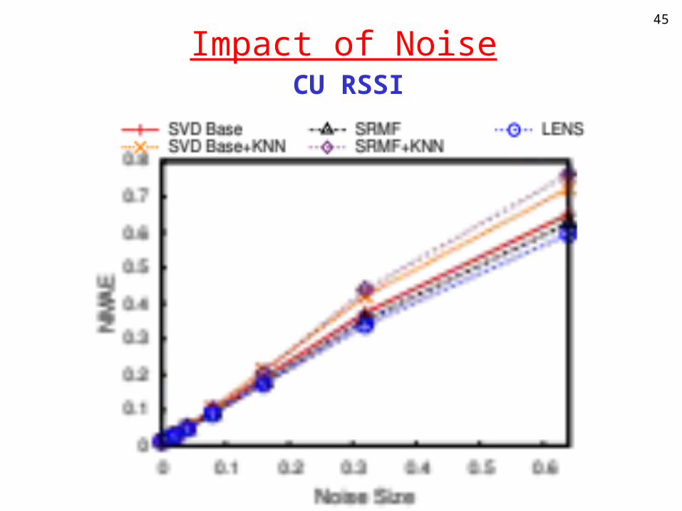
Impact of Noise45

CU RSSI

Prediction46

3G

LENS yields the lowest prediction error.

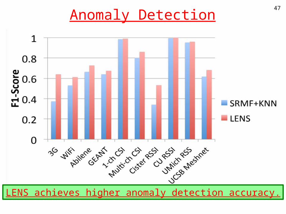
Anomaly Detection47

LENS achieves higher anomaly detection accuracy.

Computation Time48

Optimization Algorithm49

• Alternating Direction Method (ADM)– Augmented Lagrangian function

Original Objective

Lagrange multiplier

Penalty

Convergency50