lable at ScienceDirect

Progress in Nuclear Energy 54 (2012) 177e185

Contents lists avai

Progress in Nuclear Energy

journal homepage: www.elsevier .com/locate/pnucene

Robust nonlinear model predictive control for a PWR nuclear power plant

H. Eliasi a,*, M.B. Menhaj b,1, H. Davilu a

aDepartment of Nuclear Engineering, Amirkabir University of Technology, Hafez Ave., Hafez Street, PO Box: 15875-4413, Tehran, IranbDepartment of Electrical Engineering, Amirkabir University of Technology, Hafez Ave., Hafez Street, PO Box: 15875-4413, Tehran, Iran

a r t i c l e i n f o

Article history:Received 11 January 2011Received in revised form4 June 2011Accepted 8 June 2011

Keywords:PWR nuclear power plantsModel predictive controlConstrained nonlinear systemsRobust control

* Corresponding author.E-mail addresses: h_eliasi@aut.ac.ir, h_eliasi@yah

aut.ac.ir (M.B. Menhaj), davilu@aut.ac.ir (H. Davilu).1 Fax: þ98 21 66490581.

0149-1970/$ e see front matter � 2011 Elsevier Ltd.doi:10.1016/j.pnucene.2011.06.004

a b s t r a c t

One of the important operations in nuclear power plants is power control during load following in whichmany robust constraints on both input and measured variables must be satisfied. This paper proposesa robust nonlinear model predictive control for the load-following operation problem by consideringsome robust constraints on both input and output variables. The controller imposes restricted stateconstraints on the predicted trajectory during optimization which guarantees robust satisfaction of stateconstraints without restoring to a min-max optimization problem. Simulation results show that theproposed controller for the load-following operation is quite effective while the constraints are robustlykept satisfied.

� 2011 Elsevier Ltd. All rights reserved.

1. Introduction

Nuclear power plants are highly complex, nonlinear, time-varying and constrained systems and their characteristics varywith operating power levels. Changes in nuclear core reactivitywith fuel burn up generally degrade systems performance.Furthermore, if load following operating is desired, daily load cyclescan significantly change plant performance.

During the load following, input and states of nuclear reactormust be kept bounded within acceptable limits. Monitoring bothinput and states within acceptable limits is a constraint for the loadfollowing operation. Therefore, load following control for nuclearreactor is indeed a constrained control problem.

One of the most powerful tools for controlling the constrainedsystems is model predictive control (MPC) which refers to directuse of an explicit and separately identifiable model to controla constrained process. All MPC algorithms are based on themoving horizon approach known as the open-loop optimal feed-back control approach. In this method, an identified processmodel at first predicts the future response; then the currentcontrol action is determined so as to obtain the desired perfor-mance over a finite time horizon. This method has many advan-tages over the conventional infinite horizon control, because it

oo.com (H. Eliasi), menhaj@

All rights reserved.

easily handles the input, output and states constrains ina systematic manner during the design and implementation of thecontroller. Therefore, the model predictive control methodologyhas received much attention as a powerful tool for the control ofindustrial process systems (Kwon and Pearson, 1977; Richaletet al., 1978; Garcia et al., 1989; Clarke and Scattolini, 1991;Kothare et al., 1996; Lee et al., 1997; Lee et al., 1998; Khanikiet al., 2008). The MPC method has been applied to a nuclearengineering field by Kothare et al. (2000), Eliasi et al. (2007), Na(2001), and Na et al., (2003), (2004a), (2004b). Kothare et al.(2000), Eliasi et al. (2007) and Na (2001) applied the MPCmethod to control the water level of nuclear steam generators. Naet al. (2005) has also designed a model predictive controller forload-following operation of PWR reactors.

Since nuclear reactor is a nonlinear system with model uncer-tainties, which is caused by modeling, the linear MPC or nonlinearMPC may not result in a satisfactory robust dynamic performanceand closed-loop stability (Grimm et al., 2004). The need to guar-antee closed-loop stability in presence of uncertainties motivatesthe conception of Robust Nonlinear MPC which perturbations areexplicitly taken into account at controllers design. When the natureof uncertainties is known, and it is assumed to be bounded in somecompact set, the robust nonlinear MPC can be determined bysolving a min-max optimal control problem where the perfor-mance objective is optimized for the worst-case scenario (Scokaertand Mayne, 1998; Mayne et al., 2000; Mayne, 2001; Fontes andMagni, 2003). However, the use of minemax techniques islimited by the high computational burden required to solve theoptimization problem and can be applied to small-sized problems

H. Eliasi et al. / Progress in Nuclear Energy 54 (2012) 177e185178

or to processes with very slow dynamics (Lee and Yu, 1997;Bemporad et al., 2003; Magni et al., 2003). In the case of con-strained system, such as a nuclear reactor, a possibility to ensurerobust constraint satisfaction and closed-loop stability withoutresorting to min-max optimization consists in imposing restrictedstate constraints on the predicted trajectories during optimizationin order to guarantee that original constraints are fulfilled by theperturbed system for any possible realization of the uncertainties.This idea was first introduced by Chisci et al. (2001) for linearsystems and applied to nonlinear systems by Limón et al. (2002)and Raimondo and Magni (2006) and was improved by Pin et al.(2009) for discrete nonlinear systems.

The goal of this paper is to present a restricted algorithm forcontinuous systems, in order to design a robust nonlinear MPCfor load following operations of nuclear reactors such that inputand states are bounded within acceptable limits. In order toanalyze the stability properties of the closed-loop system in thepresence of bounded persistent disturbances and state-dependent uncertainties, the characterization of input-to-statestability (ISS) in terms of Lyapunov functions is used (Khalil,2002).

The outline of the paper is as follows: Section 2 describesnuclear reactor modeling with one delayed neutron group andtemperature feedback from lumped fuel and coolant temperatures.Section 3 presents the proposed robust nonlinear MPC. In Section 4,the proposed controller is applied to the nuclear reactor loadfollowing problem. Section 5 concludes the paper.

2. Nuclear reactor model

In this paper, the pressurized water reactor (PWR) modelassumes point kinetics equations with one delayed neutron groupand xenon feedback which is summarized as follows (Ben-Abdennour et al., 1992; Edwards et al., 1990; Edwards et al., 1992;Schultz, 1961):

dnr

dt¼ r� b

Lnr þ b

Lcr þwnr

dcrdt

¼ lnr � lcr þwcr

dIdt

¼ �lIIþ gIfþwI

dXdt

¼ lIIþ ðgX � sXXtÞf� lXXþwX

ddrdt

¼ GrZrr ¼ drr � sXðX� X0Þ

(2-1)

where nr denotes the neutron density relative to initial equilibriumdensity at rated condition, cr denotes the precursor density relativeto initial equilibrium density at rated condition. I and X denoteiodine and xenon concentrations respectively, f denotes fluxneutron and drr denotes reactivity due to the control rod move-ment. b and l denote one group delayed neutron yield and decayconstant, respectively, L denotes prompt neutron life time, sx

denotes microscopic thermal neutron absorption cross section ofxenon, gx and gI denote xenon and iodine yield per fission and lxand lI denote xenon and iodine decay constants, respectively. Grand Zr represent total reactivity worth of control rod and controlrod speed in units of fraction of core length per second (controlinput), respectively.

Vector w ¼ [wnr, wcr, wI, wX, 0]T is vector of bounded uncer-tainties and bounded disturbancewith jwnr j � 0:03, jwcr j � 0:03jwI j� 10�4jwX j � 10�4.

In order to convert the load following problem of nuclear reactorto the stabilization problem, we define

dnr ¼ nr � nr0dcr ¼ cr � cr0dI ¼ I� I0dX ¼ X� X0df ¼ n n0 dnr

(2-3)

where the symbol D indicates the deviation of a variable from anequilibrium value, and nr0, cr0, I0 and X0 correspond respectively tothe values of nr, cr, I and X at an equilibrium condition. n and n0denote thermal neutrons speed (cm/s) and initial equilibrium(steady-state) neutron density (1/cm3), respectively.

Consider the state vector as

x ¼ ½dnr dcr dI dX drr�T (2-4)

and u¼ Zr, then the nonlinear state-spacemodel of nuclear reactors(2-1) can be written as follows:

_x ¼ fðx;uÞ þw (2-5)

where w is bounded uncertainty and bounded disturbance vectorand f(x) is as follows:

fðxÞ ¼

2666666664

drr�sxdX�bL

dnrþ bLdcrþðnr0Þ

Ldrr�

ðnr0ÞsX

LdX

ldnr�ldcr�lIdIþgIdf

lIdIþgXdf�sXX0df�ðsXf0þlXÞdXGrZr

3777777775

(2-6)

The system output is chosen as:

y ¼ CTx; C ¼ ½1 0 0 0 0 �T (2-7)

3. Robust nonlinear MPC

In the following, main notations and basic definitions which areused in this section will be given.

3.1. Notation and basic definitions

Let R and R�0 denote the real and non-negative real numbers,respectively. The Euclidean norm is denoted as j$j. The set ofsequences w, whose values belong to a compact set W4Rm isdenoted by Mw, while wsup ¼D supw˛Wfjwjg.

Given two sets A˛Rn and B˛Rn, then the pontryagin differenceset C is defined as follows:

C ¼ AwB ¼D �x˛Rn : xþ x˛A; cx˛B

�and

A=B¼D �x˛Rn : x˛A; x;B�

Given a vector x˛Rn, dðx;AÞ¼D inffjx� xj; x˛Ag is the point toset distance from x˛Rn to A. distðA;BÞ¼D inffdðx;AÞ; x˛Bg is theminimal set-to-set distance. Given a vector h˛Rn and a positiver˛R>0, the closed ball centered in h and of radius r, is denoted asBðh; rÞ¼D fx˛Rn : jx� hj � rg. The shorthand B(r) is used when theball is centered in the origin.

Definition 1 (K-function) A function g:R�0/R�0 is of class K (ora "K-function") if it is continuous, positive definite, strictlyincreasing and g(0) ¼ 0.

Definition 2 (KN - function) A function g:R�0/R�0 is of class KN

(or a "KN-function") if it is a K-function and g(s)/N ass/N.

H. Eliasi et al. / Progress in Nuclear Energy 54 (2012) 177e185 179

Definition 3 (KL - function) A function b:R�0 � R�0/R�0 is ofclass KL, if for each fixed t � 0, bð$; tÞ is of class K and for each fixeds � 0, bðs; $Þ is decreasing and b(s,t)/0 as t/N.

Definition 4 (Positively Invariant -PI- set) The set 43Rn is saidpositively invariant for the system _x ¼ fðxðtÞÞ, if for all xð0Þ˛4, thesolution is such that xðtÞ˛4 for t > 0 (Blanchini, 1999).

Definition 5 (Controlled Invariant set) The set 43Rn is saidcontrolled invariant for the system _x ¼ fðxðtÞ;uðtÞÞ, if there existsa continuous feedback control law, u(t) ¼ F(x(t)), which assures theexistence anduniqueness of the solution onRn and it is such that4 ispositively invariant set for the closed loop system (Blanchini, 1999).

The map f:Rn � Rm/Rn is Lipschitz in x in the domain X � U, ifthere exists a positive constant Lf such that jfða;uÞ � fðb;uÞj �Lf ja� bj, for all a;b˛X, and all u˛U.

The nonlinear state-space model of nuclear reactor (2-5) can beconsidered as an uncertain nonlinear system of the following form:

_x ¼ fðxðtÞ;uðtÞ;wðtÞÞ (3-1)

where xðtÞ˛Rn is the state vector of the system and uðtÞ˛Rm is thecontrol vector. The wðtÞ˛Rw represents the bounded and statedepended uncertainties and disturbance. Control, state anduncertainty vectors are subject to the hard constraints, u˛U, x˛X,andw˛W,where U andWare convex and compact polytopes and Xis a convex and closed polyhedron. For the given system in eq. 3-1,assume that f ðxðtÞ;uðtÞÞ with fð0;0Þ ¼ 0 denote the nominalmodel used for control design purposes, such that

_x ¼ f ðxðtÞ;uðtÞÞ þ dðtÞ (3-2)

where dðtÞ¼D fðxðtÞ;uðtÞ;wðtÞÞ � fðxðtÞ;uðtÞÞ˛Rn denotes thecontinuous-time transition uncertainty. The following assumptionswill be used through the note.

Assumption 1 f is Lipschitz with respect to x for all x˛X, withconstant Lfx˛R>0.

Assumption 2 The additive transition uncertainty d(t) is limitedin time varying compact ball D, that is dðxðtÞ;uðtÞ;wðtÞÞ ˛ D ¼D BðdðjxðtÞjÞ þ mðWsupÞÞcxðtÞ˛X, }uðtÞ˛U, cwðtÞ˛ W .d and m are two K-functions. The K-function d is such thatLd ¼D minfL˛R>0 : dðjxðtÞjÞ � LjxðtÞj; cx˛Xg exists finite. It followsthat d(t) is bounded by sum of contributions: a state-dependedcomponent and a non-state-depended one. The control objectiveconsists in designing a state-feedback control law for load followingsuch that closed-loop Input-to-State Stability (ISS) is achieved andstate and control constraints are satisfy in presence of state-depended uncertainties and persistent disturbances.

3.2. Nominal NMPC

In NMPC, the input applied to the system (2-5) is usually given bythe solution of the following finite horizon open-loop optimalcontrol problem (FHOCP),which is solved at every sampling instant:

minuð$Þ

JðxðtÞ; uð$ÞÞ

subject to: _xðsÞ ¼ fðxðsÞ; uðsÞÞ; xðtÞ ¼ xðtÞuðsÞ˛U; cs˛½t; tþ Tc�uðsÞ ¼ kf ðxðsÞÞ; cs˛

�tþ Tc; tþ Tp

�xðsÞ˛X; cs˛

�t; tþ Tp

� (3-3)

with the cost function:

JðxðsÞ;uð$ÞÞ ¼Z tþTc

thðxðsÞ; uðsÞÞdsþ

Z tþTp

tþTc

h�xðsÞ; kf ðxðsÞÞ

�ds

þVf�x�tþTp

Here Tp and Tc are the prediction and the control horizon withTc � Tp. In the following, Np and Nc are number of sampling timeinstants over prediction horizon and control horizon respectivelyand defined as follows:

Np ¼ Tps

(3-4)

Nc ¼ Tcs

(3-5)

where s is sampling period.The bar denotes predicted variables, i.e. xð$Þ is the solution of (3-

3) driven by the input uð$Þ˛U with initial condition x (t). kf is anauxiliary control law. The distinction between the real system statex(t) of (3-1) and the predicted state, x�, in the controller is necessarysince due the moving horizon nature, even in the nominal case, thepredicted state will differ from the real states at least after onesampling instant.

Assumption 3 The cost function J is such that h ðjxjÞ � hðx;uÞ;cx ˛ X, cu ˛ U where h�is KN� function. Moreover, h is Lipschitzwith respect to x and u in X � U, with Lipschitz constants Lhx ˛ R�0andLhu ˛ R�0, respectively.

According to the receding horizon approach, the state-feedbackMPC control low is derived by solving FHOCP at every samplingtime instant tk and applying the control signaluðtÞ ¼ uotk;tkþ1

,t˛ðtk; tkþ1Þ where uo

tk;tkþ1is the first part of the optimal sig-

nalu+tk;tkþNp. In so doing, one implicitly defines the sampled state

feedback control lowuðtÞ ¼ kMPCðt; xtÞ; t˛ðtk; tkþ1Þ. In thefollowing, XMPC will denote the set containing all the state vectorsfor which a feasible control sequence exists, i.e. a control sequenceuotk;tkþNp

, satisfying all the constraints of the FHOCP.

3.3. Robust NMPC strategy

The constraints (3-3) involve only the nominal prediction.Therefore, they do not provide any guarantee that the true systemstate and input will satisfy the constraints due to the presence ofthe state-depended uncertainties and disturbance. Hence nominalNMPC, as well as many standard prediction control algorithms, canlose feasibility and hence its guarantee of stability.

In order to formulate the robust MPC algorithm, let introducethe following further assumptions:

Assumption 4. Given an auxiliary control law,kf, and a set Xf, thedesign parameters Vf is such that

1. Xf 4 X, Xf closed, 0 ˛ Xf2. kf(x) ˛ U, for all x ˛ Xf; kf(x) is Lipschitz in Xf, with constant

Lkf ˛ R>03. the closed loop map f ðx; kf ðxÞÞ, is Lipschitz in Xf with constant

Lfc ˛ R>04. Xf is a controlled invariant set for _x ¼ f ðx; kf ðxÞÞ with control

law u(t) ¼ kf(x(t))5. Vf(x) is Lipschitz in Xf, with constant LVf ˛ R>0.6. ðVVf ÞT f ðx; kf ðxÞÞ � �hðx; kf ðxÞÞ; for all x ˛ Xf and T > 07. ~u½t;tþTp� ¼D ½kf ðxðsÞÞ�; s˛½t; t þ Tp�; with xðtÞ ¼ xðtÞ is a feasible

control sequence for FHOCP, for all x(t) ˛ Xf.

Assumption 5 The robust terminal constraint set of the FHOCP,XTc, is chosen such that:

a) for all x˛XTc, the state can be steered to Xf in Tp�Tc secondunder the nominal dynamics in closed-loop with auxiliarycontrol law kf ;

Table 1Parameters of the nuclear reactor at the middle of fuel cycle in 100% nominal power.

Parameter Value

Thermal Power 2500 MWInitial equilibrium relative neutron density (nr0) 1Mean velocity of thermal neutron (y) 2.2 � 105 cm/sMicroscopic absorption cross section of Xe (sx) 2.36 � 10�18 cm2

Fractional fission yield of Xe (gX) 0.00228Fractional fission yield of I (gI) 0.0639Decay constant of Xe (lx) 2.08 � 10�5 s�1

Decay constant of I (lI) 2.88 � 10�5 s�1

Mean velocity of thermal neutron (y) 2.2 � 105 cm/sMicroscopic absorption cross section of Xe (sx) 2.36 � 10�18 cm2

Total delayed neutron fraction (b) 6.019 � 10�3

Effective prompt neutron life time (L) 2 � 10�5 sRadioactive decay constant of one group neutron

precursor (l)0.150 s�1

Total reactivity worth of control rod (G) 14.5 � 10�3 Dk/k

H. Eliasi et al. / Progress in Nuclear Energy 54 (2012) 177e185180

b) for each Dt > 0, there exists a positive scalar e˛R> 0 such thatR tþDtt fðxðsÞ; kf ðxðsÞÞÞds˛ XNcwBðeÞ;cxt˛XTc,

For implementing robust NMPC, the original constraints (3-3)must be replaced with more stringent ones which preserve feasi-bility despite the presence of uncertainties and disturbances.Therefore, under assumption 2, for given x(t), a norm-bound on thestate prediction error will be derived. Subsequently, it is shown thatthe satisfaction of the original state constraints is ensured, for anyadmissible uncertainties and disturbances sequence, by imposingrestraints to the predicted open-loop trajectories.

Lemma 1: Under assumptions 1 and 2, for the given state vectorx(t) at the time t, let a control sequence, ut;tþTc

be feasible withrespect to the restricted state constraints of the FHOCP, XðsÞjtcomputed as follows:

XðsÞjt ¼D XwBðrðsÞjtÞ (3-6)

Wherer ðtÞ ¼D 0 _rðsÞjt ¼

�Ld þ Lfx

�rðsÞjt þ mþ Ld

��xðsÞjt��; s˛½t; tþ Tc�

(3-7)With m ¼ mðwsupÞThen, the sequence ut;tþNc

, applied to the perturbed system (3-1),guarantees x(s)˛X, s˛[t,tþTc], cx(t)˛XMPC,cw˛W.

Proof: For given x(t), the prediction error over control horizon isintroducedby e ðsÞ ¼D xðsÞ � xðsÞjt ; thenderivative of prediction erroris _e ðsÞ¼D _xðsÞ � _xðsÞjt; an upper bound for this derivative is as below:

j _eðsÞjt j ¼ f�xðsÞ;uðsÞjt

þdðsÞ� f�xðsÞjt ;uðsÞjt

�Lfx

��eðsÞjt��þjdðsÞj �Lfx��eðsÞjt��þmþLdjxðsÞj

��LfxþLd

���eðsÞjt��þmþLd��xðsÞjt�� (3-8)

Finally, comparing 3-8 with 3-7, it follows that j _eðsÞjt j � _rðsÞjt .Since eðsÞ and rðsÞ are zero for s¼ t, jeðsÞjt j � rðsÞjt is resulted,which in turn proves the statement.

Thus, the proposed robust NMPC based on restricted constraintsis derived from the following optimization problem:

minuð,Þ

JðxðsÞ;uð$ÞÞ ¼Z tþTc

thðxðsÞ;uðsÞÞds

þZ tþTp

tþTc

h�xðsÞ; kf ðxðsÞÞ

�ds

þ Vf�x�tþ Tp

(3-9)

subject to: _xðsÞ ¼ fðxðsÞ;uðsÞÞ; xðtÞ ¼ xðtÞ

uðsÞ˛U;cs˛½t; tþTc�uðsÞ ¼ kf ðxðsÞÞ; cs˛

�tþTc; tþTp

�;

xðtþTcjtÞ˛XTc

r�t�¼ 0 _rðsÞjt ¼

�LdþLfx

�rðsÞjtþmþLd

��xðsÞjt��; s˛½t;tþTc�;xðsÞjt ¼ XwBðrðsÞjtÞ;xðsÞjt˛xðsÞjt; cs˛½t; tþTc�;

3.4. Regional input to state stability properties

In the following, for the analysis of the robust stability ofproposed NMPC, we use of the regional Input-to-State practicalstability (ISpS) property.

Consider that system (3-1) is controlled by certain control lawu(t)¼kMPC (x(t)), then the closed-loop system can be expressed asfollows:

_xðtÞ ¼ fMPCðxðtÞ;wðtÞÞ; t � 0 (3-10)

Definition 6. (RPI set): A set E3Rn is a Robust Positively Invariant(RPI) for system (3-10), if for all x(t0)˛E and all w(t)˛W, the solu-tion is such that x(t)˛E for t > t0.

Definition 7. (predecessor set): Given the set P3X, the prede-cessor set for _x ¼ f ðx;uÞ from P in time Dt,U(P), is the set of allvectors x(t) in Rn for which there exists an admissible control inputwhich will guarantee that the system will be driven to P in Dt,namely, x(tþDt)˛P.

Definition 8. (Regional ISpS and ISS)e Given a compact set E3Rn,if E is RPI for (3-10) and if there exists a KLe function b, a K-functiong and a positive number c˛R>0 such that:

jxðtÞ;xðt0Þ;wj � max�bðjxðt0Þj; tÞ þ gð����wðtÞ��jNÞ�þ c (3-11)

for t > 0 and c x(t0)˛E, then the system (3-10), with w˛W, issaid to be Input-to-State practical Stable (ISpS) in E. In the case thatc ¼ 0, the system (3-8) is said to be Input-to-State Stable (ISS) in E.

Definition 9. (ISS and ISpS Lyapunov functions (Magni et al.,2006)):

Consider that E is an RPI set containing the origin in its interior.A function V: Rn/R�0 is called an ISpS-Lyapunov function in E forsystem (3-10), if there exists a compact set U4E, including theorigin as an interior point, suitable KN -functions a1, a2, a3, a4 andtwo positive constants c1, c2 such that:

VðxÞ � a1ðjxjÞ; cx˛E (3-12)

VðxÞ � a2ðjxjÞ þ c1; cx˛U (3-13)

And for all x ˛ X, w˛W;

_VðxðtÞÞ � �a3ðjxjÞ þ a4ðjwjÞ þ c2; cx˛E (3-14)

Whenever inequalities (3-12), (3-13) and (3-14) are satisfied withc1 ¼ c2 ¼ 0, the function V is an ISS-Lyapunov function in E.

Then, the following important results can be proven.

Theorem 1 If system (3-10) admits an ISpS-Lyapunov function inE, that is regional ISpS in E, (Limon et al., 2009).

Robust stability of proposed robust NMPC can now be estab-lished by the following theorem.

Theorem 2 (Robust ISpS stability of proposed robust NMPC) e

System (3-1) controlled by the nominal model predictive controller

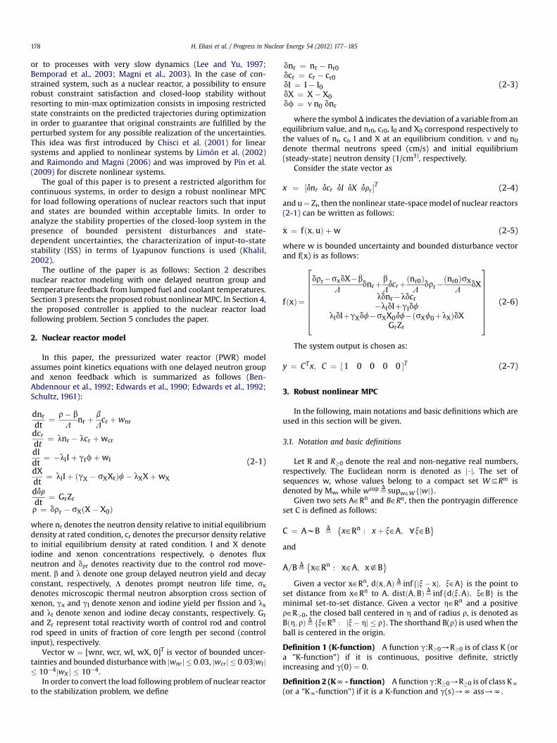
Fig. 1. Case A1: Full power operation for 100%e80% power change. (a) Relative nuclear power. (b) Control rod speed.

H. Eliasi et al. / Progress in Nuclear Energy 54 (2012) 177e185 181

u(t)¼kMPC(x(t)) will be regional ISpS in E ¼ XMPC with respect tow˛W and the following assumption [Appendix A]:

a1ðsÞ ¼ h ðsÞ (3-15)

a2ðsÞ ¼ LVf ðsÞ (3-16)

c1 ¼ 0 (3-17)

a3ðsÞ¼hðsÞ�"Lhx

eTcLfx�1

Lfx

!þ�LhxþLhuLkf

� eðTp�TcÞLfc�1Lfc

!

eTcLfx þLVfeðTp�TcÞLfceTcLfx

#dðsÞ ð3�18Þ

a4ðsÞ ¼"Lhx

eTcLfx � 1

Lfx

!þ�Lhx þ LhuLkf

� eðTp�TcÞLfc � 1Lfc

!eTcLfx

þLVfeðTp�TcÞLfceTcLfx

imðsÞ (3-19)

C2 ¼"�

Lhx þ LhuLkf� eðTp�TcÞLfc � 1

Lfc

!þ LVf

eðTp�TcÞLfc#

�max���x� x

��; ðx; xÞ˛XTc � XTc4BnðdÞ�þ Lhu �maxfju�wj; ðu;wÞ˛U� Ug (3-20)

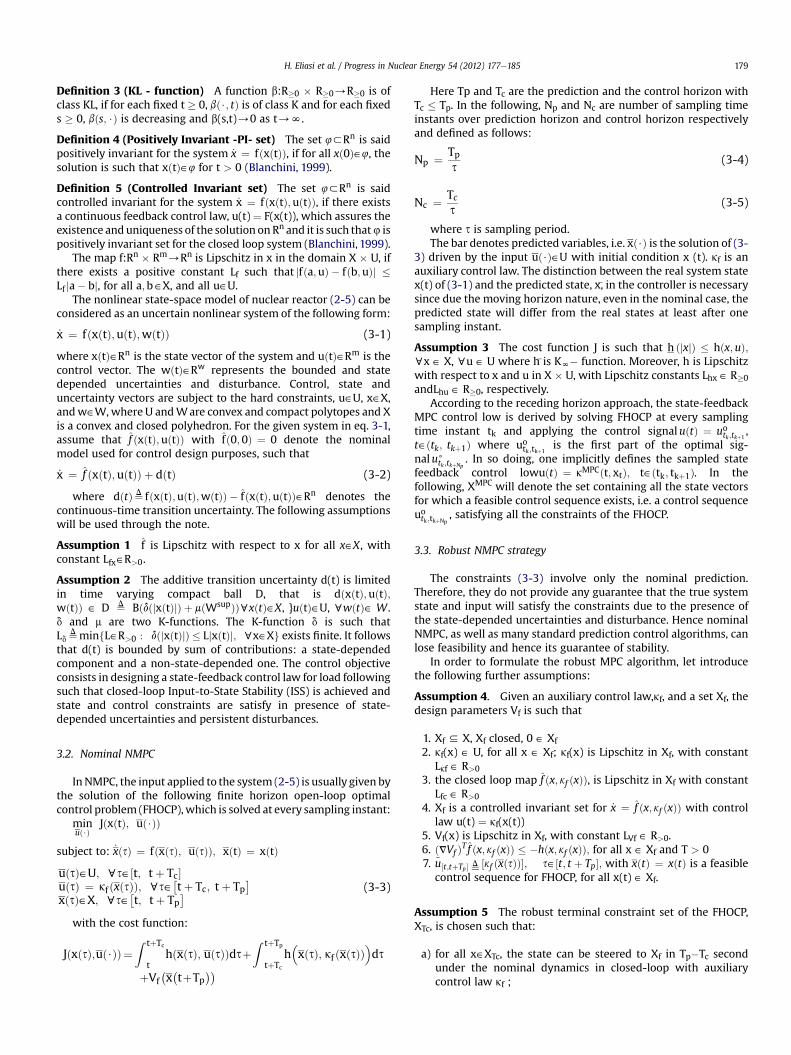
Fig. 2. Case A2: Full power operation for 80%e100% power ch

The ISpS-Lyapunov function is the optimal value of costfunction,VðxðtÞÞ ¼ JðxðtÞ;uo

t;tþTpÞ.

4. Application to the nuclear reactor load following

In this section, the proposed algorithm is applied to the loadfollowing operation problem. It was assumed that initially thecontrolled plant was at an equilibrium condition. The samplingperiod is 5s. In this paper assumed that maximum speed of controlrod (u ¼ Zr) is 2.5 � 10�1 fraction of core length per second.Therefore, the control constraint set, U, is considered asU ¼D fu˛R : juj � 2:5� 10�1g. The Lipschitz constant of the systemis Lfx ¼ 2.175 � 10�1. The parameters of the nuclear reactor at themiddle of fuel cycle in 100% nominal power are given in Table 1.

Three case studies are considered to show the performance ofthe proposed controller:

Case A Full power operation

1. 100%e80% power level change.2. 80%e100% power level change.

Case B Low power operation

1. 40%e20% power level change.2. 20%e 40% power level change.

Case C Emergency operation

1. 100%e20% power level change (Load Rejection).2. 20%e100% power level change (Load Lift)

ange. (a) Relative nuclear power. (b) Control rod speed.

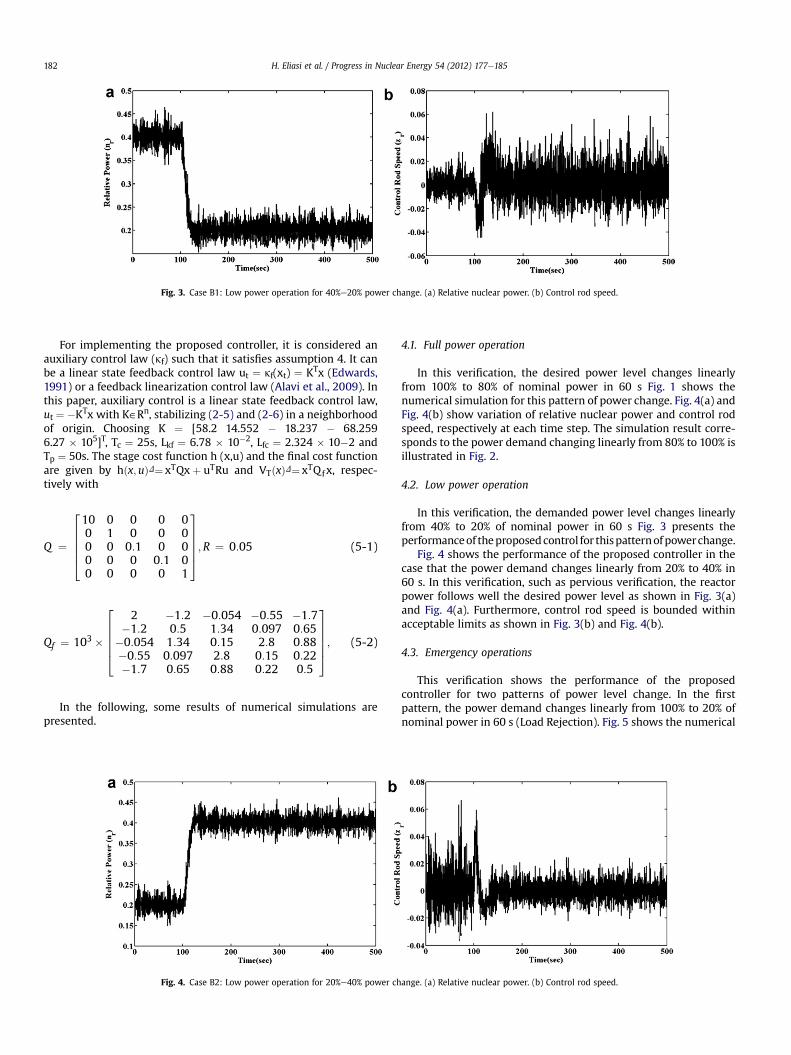
Fig. 3. Case B1: Low power operation for 40%e20% power change. (a) Relative nuclear power. (b) Control rod speed.

H. Eliasi et al. / Progress in Nuclear Energy 54 (2012) 177e185182

For implementing the proposed controller, it is considered anauxiliary control law (kf) such that it satisfies assumption 4. It canbe a linear state feedback control law ut ¼ kf(xt) ¼ KTx (Edwards,1991) or a feedback linearization control law (Alavi et al., 2009). Inthis paper, auxiliary control is a linear state feedback control law,ut ¼ �KTx with K˛Rn, stabilizing (2-5) and (2-6) in a neighborhoodof origin. Choosing K ¼ [58.2 14.552 � 18.237 � 68.2596.27 � 105]T, Tc ¼ 25s, Lkf ¼ 6.78 � 10�2, Lfc ¼ 2.324 � 10�2 andTp ¼ 50s. The stage cost function h (x,u) and the final cost functionare given by hðx;uÞD¼ xTQxþ uTRu and VTðxÞD¼ xTQfx, respec-tively with

Q ¼

26666410 0 0 0 00 1 0 0 00 0 0:1 0 00 0 0 0:1 00 0 0 0 1

377775;R ¼ 0:05 (5-1)

Qf ¼ 103 �

266664

2 �1:2 �0:054 �0:55 �1:7�1:2 0:5 1:34 0:097 0:65

�0:054 1:34 0:15 2:8 0:88�0:55 0:097 2:8 0:15 0:22�1:7 0:65 0:88 0:22 0:5

377775; (5-2)

In the following, some results of numerical simulations arepresented.

Fig. 4. Case B2: Low power operation for 20%e40% power ch

4.1. Full power operation

In this verification, the desired power level changes linearlyfrom 100% to 80% of nominal power in 60 s Fig. 1 shows thenumerical simulation for this pattern of power change. Fig. 4(a) andFig. 4(b) show variation of relative nuclear power and control rodspeed, respectively at each time step. The simulation result corre-sponds to the power demand changing linearly from 80% to 100% isillustrated in Fig. 2.

4.2. Low power operation

In this verification, the demanded power level changes linearlyfrom 40% to 20% of nominal power in 60 s Fig. 3 presents theperformanceof theproposedcontrol for thispatternofpowerchange.

Fig. 4 shows the performance of the proposed controller in thecase that the power demand changes linearly from 20% to 40% in60 s. In this verification, such as pervious verification, the reactorpower follows well the desired power level as shown in Fig. 3(a)and Fig. 4(a). Furthermore, control rod speed is bounded withinacceptable limits as shown in Fig. 3(b) and Fig. 4(b).

4.3. Emergency operations

This verification shows the performance of the proposedcontroller for two patterns of power level change. In the firstpattern, the power demand changes linearly from 100% to 20% ofnominal power in 60 s (Load Rejection). Fig. 5 shows the numerical

ange. (a) Relative nuclear power. (b) Control rod speed.

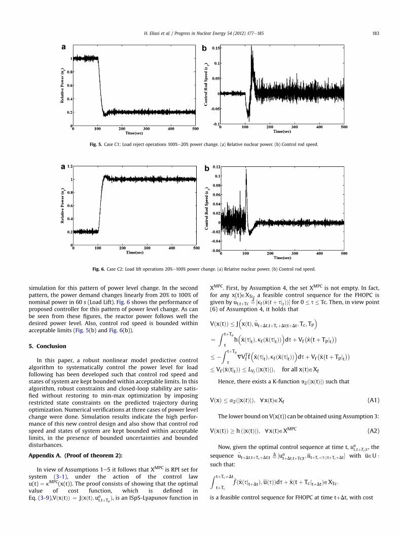
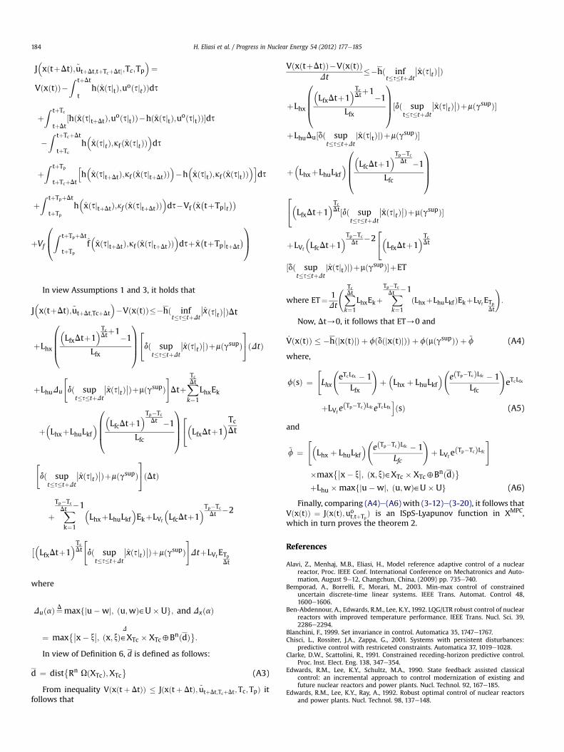
Fig. 5. Case C1: Load reject operations 100%e20% power change. (a) Relative nuclear power. (b) Control rod speed.

Fig. 6. Case C2: Load lift operations 20%e100% power change. (a) Relative nuclear power. (b) Control rod speed.

H. Eliasi et al. / Progress in Nuclear Energy 54 (2012) 177e185 183

simulation for this pattern of power level change. In the secondpattern, the power demand changes linearly from 20% to 100% ofnominal power in 60 s (Load Lift). Fig. 6 shows the performance ofproposed controller for this pattern of power level change. As canbe seen from these figures, the reactor power follows well thedesired power level. Also, control rod speed is bounded withinacceptable limits (Fig. 5(b) and Fig. 6(b)).

5. Conclusion

In this paper, a robust nonlinear model predictive controlalgorithm to systematically control the power level for loadfollowing has been developed such that control rod speed andstates of system are kept bounded within acceptable limits. In thisalgorithm, robust constraints and closed-loop stability are satis-fied without restoring to min-max optimization by imposingrestricted state constraints on the predicted trajectory duringoptimization. Numerical verifications at three cases of power levelchange were done. Simulation results indicate the high perfor-mance of this new control design and also show that control rodspeed and states of system are kept bounded within acceptablelimits, in the presence of bounded uncertainties and boundeddisturbances.

Appendix A. (Proof of theorem 2):

In view of Assumptions 1e5 it follows that XMPC is RPI set forsystem (3-1), under the action of the control lawu(t) ¼ kMPC(x(t)). The proof consists of showing that the optimalvalue of cost function, which is defined inEq. (3-9),VðxðtÞÞ ¼ JðxðtÞ;uot;tþTp

Þ, is an ISpS-Lyapunov function in

XMPC. First, by Assumption 4, the set XMPC is not empty. In fact,for any x(t)˛XTc, a feasible control sequence for the FHOPC isgiven by ~ut;tþTc ¼D ½kf ðxðt þ sjtÞÞ� for 0 � s � Tc. Then, in view point(6) of Assumption 4, it holds that

VðxðtÞÞ � J�xðtÞ; ~utþDt;tþTcþDtjtþDt;Tc; TP

�

¼Z tþTp

th�xðsjtÞ; kf ðxðsjtÞÞ

�dsþ Vf

�x�tþ Tpjt

� �Z tþTp

tVVT

f f�xðsjtÞ; kf ðxðsjtÞÞ

�dsþ Vf

�x�tþ Tpjt

� Vf ðxðtjtÞÞ � LVf

ðjxðtÞjÞ; for all xðtÞ˛Xf

Hence, there exists a K-function a2ðjxðtÞjÞ such that

VðxÞ � a2ðjxðtÞjÞ; cxðtÞ˛Xf (A1)

The lower bound on V(x(t)) can be obtained using Assumption 3:

VðxðtÞÞ � h ðjxðtÞjÞ; cxðtÞ˛XMPC (A2)

Now, given the optimal control sequence at time t, uot;tþTcjt , thesequence ~utþDt;tþTcþDtjt ¼D ½uotþDt;tþTcjt;utþTc<s�tþTcþDt� with u˛U :

such that:

Z tþTcþDt

tþTc

f ðxðsjtþDtÞ;uðsÞÞdsþ xðtþ TcjtþDtÞ˛XTc:

is a feasible control sequence for FHOPC at time tþDt, with cost

H. Eliasi et al. / Progress in Nuclear Energy 54 (2012) 177e185184

J�xðtþDtÞ;~utþDt;tþTcþDtj;Tc;Tp

�¼

VðxðtÞÞ�Z tþDt

thðxðsjtÞ;uoðsjtÞÞds

þZ tþTc

½hðxðsjtþDtÞ;uoðsjtÞÞ�hðxðsjtÞ;uoðsjtÞÞ�ds

tþDt

�Z tþTcþDt

tþTc

h�xðsjtÞ;kf ðxðsjtÞÞ

�ds

þZ tþTp h

h�xðsjtþDtÞ;kf ðxðsjtþDtÞÞ

��h�xðsjtÞ;kf ðxðsjtÞÞ

�ids

tþTcþDt

þZ tþTpþDt

h�xðsjtþDtÞ;kf ðxðsjtþDtÞÞ

�ds�Vf

�x�tþTpjt

tþTp0BZ tþTpþDt � � � 1C þVf@

tþTp

f xðsjtþDtÞ;kf ðxðsjtþDtÞÞ dsþ x tþTpjtþDt A

In view Assumptions 1 and 3, it holds that

J�xðtþDtÞ;~utþDt;TcþDt

��VðxðtÞÞ��hð inf

t�s�tþDt

��xðsjtÞ��ÞDt

þLhx

0BBB@�LfxDtþ1

�TcDtþ1�1

Lfx

1CCCA24dð sup

t�s�tþDt

��xðsjtÞ��ÞþmðgsupÞ35ðDtÞ

þLhuDu

"dð sup

t�s�tþDt

��xðsjtÞ��ÞþmðgsupÞ#Dtþ

XTcDt

k¼1

LhxEk

þ�LhxþLhuLkf

�0BBB@�LfcDtþ1

�Tp�Tc

Dt �1

Lfc

1CCCA24�LfxDtþ1

�TcDt

"dð sup

t�s�tþDt

��xðsjtÞ��ÞþmðgsupÞ35ðDtÞ

þXTp�Tc

Dt �1

k¼1

�LhxþLhuLkf

�EkþLVf

�LfcDtþ1

�Tp�Tc

Dt �2

��LfxDtþ1

�TcDt

"dð sup

t�s�tþDt

��xðsjtÞ��ÞþmðgsupÞ#DtþLVf

ETp

Dt

where

DuðaÞ¼D maxfju�wj; ðu;wÞ˛U� Ug; and DxðaÞ

¼ max���x� x

��; ðx; xÞ˛XTc � XTc4BnðdÞ�:D

In view of Definition 6, d is defined as follows:

d ¼ dist�Rn UðXTcÞ;XTc

�(A3)

From inequality Vðxðtþ DtÞÞ � Jðxðtþ DtÞ; ~utþDt;TcþDt;Tc; TpÞ itfollows that

VðxðtþDtÞÞ�VðxðtÞÞ��hð inf��xðsjtÞ��Þ

Dt t�s�tþDt

þLhx

0BBB@�LfxDtþ1

�TcDtþ1�1

Lfx

1CCCA½dð sup

t�s�tþDt

��xðsjtÞ��ÞþmðgsupÞ�

þLhuDu½dð supt�s�tþDt

jxðsjtÞjÞþmðgsupÞ�

þ�LhxþLhuLkf

�0BBB@�LfcDtþ1

�Tp�Tc

Dt �1

Lfc

1CCCA

24�LfxDtþ1

�TcDt½dð sup

t�s�tþDt

��xðsjtÞ��ÞþmðgsupÞ�

þLVf

�LfcDtþ1

�Tp�Tc

Dt �224�LfxDtþ1

�TcDt

½dð supt�s�tþDt

jxðsjtÞjÞþmðgsupÞ�þET

where ET¼ 1Dt

XTcDt

k¼1

LhxEkþXTp�Tc

Dt �1

k¼1

ðLhxþLhuLkf ÞEkþLVfETp

Dt

!:

Now, Dt/0, it follows that ET/0 and

_VðxðtÞÞ � �hðjxðtÞjÞ þ fðdðjxðtÞjÞÞ þ fðmðgsupÞÞ þ ~f (A4)

where,

fðsÞ ¼"Lhx

eTcLfx � 1

Lfx

!þ�Lhx þ LhuLkf

� eðTp�TcÞLfc � 1Lfc

!eTcLfx

þLVfeðTp�TcÞLfceTcLfx

iðsÞ (A5)

and

~f ¼"�

Lhx þ LhuLkf� eðTp�TcÞLfc � 1

Lfc

!þ LVf

eðTp�TcÞLfc#

�max���x� x

��; ðx; xÞ˛XTc � XTc4BnðdÞ�þLhu �maxfju�wj; ðu;wÞ˛U� Ug (A6)

Finally, comparing (A4)e(A6) with (3-12)e(3-20), it follows thatVðxðtÞÞ ¼ JðxðtÞ;uo

t;tþTpÞ is an ISpS-Lyapunov function in XMPC,

which in turn proves the theorem 2.

References

Alavi, Z., Menhaj, M.B., Eliasi, H., Model reference adaptive control of a nuclearreactor, Proc. IEEE Conf. International Conference on Mechatronics and Auto-mation, August 9e12, Changchun, China, (2009) pp. 735e740.

Bemporad, A., Borrelli, F., Morari, M., 2003. Min-max control of constraineduncertain discrete-time linear systems. IEEE Trans. Automat. Control 48,1600e1606.

Ben-Abdennour, A., Edwards, R.M., Lee, K.Y., 1992. LQG/LTR robust control of nuclearreactors with improved temperature performance. IEEE Trans. Nucl. Sci. 39,2286e2294.

Blanchini, F., 1999. Set invariance in control. Automatica 35, 1747e1767.Chisci, L., Rossiter, J.A., Zappa, G., 2001. Systems with persistent disturbances:

predictive control with restriceted constraints. Automatica 37, 1019e1028.Clarke, D.W., Scattolini, R., 1991. Constrained receding-horizon predictive control.

Proc. Inst. Elect. Eng. 138, 347e354.Edwards, R.M., Lee, K.Y., Schultz, M.A., 1990. State feedback assisted classical

control: an incremental approach to control modernization of existing andfuture nuclear reactors and power plants. Nucl. Technol. 92, 167e185.

Edwards, R.M., Lee, K.Y., Ray, A., 1992. Robust optimal control of nuclear reactorsand power plants. Nucl. Technol. 98, 137e148.

H. Eliasi et al. / Progress in Nuclear Energy 54 (2012) 177e185 185

Edwards, R.M., Robust Optimal Control of Nuclear Reactors. PhD Thesis in NuclearEngineering, The Pennsylvania State University, University Park, 1991.

Eliasi, H., Davilu, H., Menhaj, M.B., 2007. Adaptive fuzzy model based predictivecontrol of nuclear steam generators. Nucl. Eng. Des. 237, 668e676.

Fontes, F.A.C.C., Magni, L., 2003. Min-max model predictive control of nonlinearsystems using discontinuous feedbacks. IEEE Trans. Auto. Control 48, 1750e1755.

Garcia, C.E., Prett, D.M., Morari, M., 1989. Model predictive control: theory andpracticeda survey. Automatica 25, 335e348.

Grimm, G., Messina, M.J., Tuna, S.E., Teel, A.R., 2004. Examples when nonlinearmodel predictive control is nonrobust. Automatica 40, 1729e1738.

Khalil, H.K., 2002. Nonlinear Systems, third ed. Prentice-Hall, Englewood Cliffs.Khaniki, R.M., Menhaj, M.B., Eliasi, H., 2008. Generalized predictive control of batch

polymerization reactor. World Acad. Sci. Eng. Technol. 1, 51e56.Kothare, M.V., Balakrishnan, V., Morari, M., 1996. Robust constrained model

predictive control using linear matrix inequality. Automatica 32, 1361e1379.Kothare, M., Mettler, V.B., Morari, M., Bendotti, P., Falinower, C.M., 2000. Level

control in the steam generator of a nuclear power plant. IEEE Trans. ControlSyst. Technol., 55e69.

Kwon, W.H., Pearson, A.E., 1977. A modified quadratic cost problem and feedbackstabilization of a linear system. IEEE Trans. Automat. Control, 838e842.

Lee, J., Yu, Z., 1997. Worst-case formulations of model predictive control for systemswith bounded parameters. Automatica 33, 763e781.

Lee, J.W., Kwon, W.H., Lee, J.H., 1997. Receding horizon H tracking control for time-varying discrete linear systems. Int. J. Control 68, 385e399.

Lee, J.W., Kwon, W.H., Choi, J., 1998. On stability of constrained receding horizoncontrol with finite terminal weighting matrix. Automatica 34, 1607e1612.

Limón, D., Alamo, T., Camacho, E.F., 2002. Input-to-state stable MPC for constraineddiscrete-time nonlinear systems with bounded additive uncertainties. Proc.IEEE Conf. Decis. Control, 4619e4624.

Limon, D., Alamo, T., Raimondo, D.M., Munoz de la Pena, D., Bravo, J.M.,Ferramosca, A., Camacho, E.F., 2009. Input-to-state stability: a unifying frame-work for robust model predictive control. In: Magni, L., Raimondo, D.M.,Allgöwer, F. (Eds.), Nonlinear Model Predictive Control-Towards New Chal-lenging Applications. Springer-Verlag, Berlin, Heidelberg, pp. 1e26.

Magni, L., De Nicolao, G., Scattolini, R., Allgöwer, F., 2003. Robust model predictivecontrol of nonlinear discrete-time systems. Int. J. Robust Nonlin. Control 13,229e246.

Magni, L., Raimondo, D.M., Scattolini, R., 2006. Regional input-to-state stability fornonlinear model predictive control. IEEE Trans. Automat. Control 51,1548e1553.

Mayne, D.Q., Rawlings, J.B., Rao, C.V., Scokaert, P.O.M., 2000. Constrained modelpredictive control: stability and optimality. Automatica 36, 789e814.

Mayne, D.Q., 2001. Control of constrained dynamic systems. Eur. J. Control 7, 87e99.Na, M.G., Shin, S.H., Kim, W.C., 2003. A model predictive controller for nuclear

reactor power. J. Kor. Nucl. Soc. 35, 399e411.Na, M.G., Jung, D.W., Lee, S.M., 2004a. A receding horizon controller with

a parameter estimator for nuclear reactor power distribution. Nucl. Sci. Eng.148, 153e161.

Na, M.G., Jung, D.W., Shin, S.H., Lee, S.M., Lee, Y.J., Jang, J.W., Lee, K.B., 2004b. Designof a nuclear reactor controller using a model predictive control method. KSMEInt. J. 18, 2080e2094.

Na, M.G., Jung, D.W., Shin, S.H., Jang, J.W., Lee, K.B., Lee, Y.J., 2005. A modelpredictive controller for load-following operation of PWR reactors. IEEE Trans.Nucl. Sci. 52, 1009e1020.

Na, M.G., 2001. A model predictive controller for the water level of nuclear steamgenerators. J. Kor. Nucl. Soc. 33, 102e110.

Pin, G., Raimondo, D.M., Magni, L., Parisini, T., 2009. Robust model predictive controlof nonlinear systems with bounded and state-dependent uncertainties. IEEETrans. Automat. Control 54, 1681e1687.

Raimondo, D.M., Magni, L., 2006. A Robust Model Predictive Control Algorithm forNonlinear Systems with Low Computational Burden. IFAC Workshop onNonlinear Model Predictive Control for Fast Systems, Grenoble, France.

Richalet, J., Rault, A., Testud, J.L., Papon, J., 1978. Model predictive heuristic control:applications to industrial processes. Automatica 14, 413e428.

Schultz, M.A., 1961. Control of Nuclear Reactors and Power Plants, second ed.McGraw-Hill, New York.

Scokaert, P.O.M., Mayne, D.Q., 1998. Min-max feedback model predictive control forconstrained linear systems. IEEE Trans. Automat. Control 43, 1136e1142.