Robust On-Manifold Optimization for Uncooperative Space

Relative Navigation with a Single Camera

Duarte Rondao†

Cranfield University, Defence Academy of the United Kingdom, SN6 8LA Shrivenham, United Kingdom

Nabil Aouf‡

City University of London, ECV1 0HB London, United Kingdom

Mark A. Richardson§

Cranfield University, Defence Academy of the United Kingdom, SN6 8LA Shrivenham, United Kingdom

Vincent Dubanchet¶

Thales Alenia Space, 06150 Cannes, France

Optical cameras are gaining popularity as the suitable sensor for relative navigation in space

due to their attractive sizing, power and cost properties when compared to conventional flight

hardware or costly laser-based systems. However, a camera cannot infer depth information on

its own, which is often solved by introducing complementary sensors or a second camera. In this

paper, an innovative model-based approach is demonstrated to estimate the six-dimensional

pose of a target relative to the chaser spacecraft using solely a monocular setup. The observed

facet of the target is tackled as a classification problem, where the three-dimensional shape

is learned offline using Gaussian mixture modeling. The estimate is refined by minimizing

two different robust loss functions based on local feature correspondences. The resulting

pseudo-measurements are processed and fused with an extended Kalman filter. The entire

optimization framework is designed to operate directly on the SE(3) manifold, uncoupling the

process and measurement models from the global attitude state representation. It is validated

on realistic synthetic and laboratory datasets of a rendezvous trajectory with the complex

spacecraft Envisat, demonstrating estimation of the relative pose with high accuracy over full

tumbling motion. Further evaluation is performed on the open-source SPEED dataset.

Presented as paper 2018-2100 at the AIAA Guidance, Navigation, and Control Conference, Kissimmee, FL, 8–12 January 2018; submitted to

AIAA Journal of Guidance, Control, and Dynamics 1 September 2019; first revision received 31 July 2020; second revision received 19 December

2020; accepted for publication 22 December 2020.†PhD Candidate, Centre for Electronic Warfare, Information and Cyber.‡Professor of Robotics and Autonomous Systems, Department of Electrical and Electronic Engineering.§Professor of Electronic Warfare, Centre for Electronic Warfare, Information and Cyber.¶R&D Engineer in AOCS and Robotics, CCPIF/AP-R&T.

I. Introduction

The concept of using optical sensors for spacecraft navigation has originated concurrently to the need for developing

autonomous operations. The main rationale behind is twofold: the acquisition and processing of images is relatively

simple enough to be self-contained on-board the spacecraft, avoiding the requirement of ground processing the data; and

the same sensor feeds used for imaging detection and recognition can be used for navigation and mapping, alleviating

additional sensors size and cost constraints. The maiden voyage of autonomous navigation was the Deep Space 1

(DS1) mission [1], which culminated in a fly-by with comet 19P/Borrelly in 2001. More recently, in 2014 the Rosetta

mission [2] used optical navigation to rendezvous with the comet 67P/Churyumov–Gerasimenko. Historically, passive

camera-based navigation has been reserved for orbit determination, cruise, and fly-by sequences. For proximity

operations to small bodies, such as rendezvous, docking, or landing, the full relative pose is typically required. The

difficulty of these scenarios is amplified when the target is uncooperative, meaning it does not relay direct information

about its state. This is often overcome by resorting to more precise active sensors, such as Lidar, which have the

advantage of supplying range information and being invariant to illumination changes [3, 4]. In addition to asteroids,

Lidar has also been successfully used for relative navigation with artificial satellites [5] and developments in the field

continue being made [6], but it remains challenging to integrate in on-board systems due to size and power constraints.

The motivation is therefore set to increase the technology readiness level of passive optical navigation through the

development of supporting image processing (IP) techniques, in order to make it a viable, lower-costing alternative to

active systems for the close range relative navigation problem. This is of paramount importance for proximity operations

missions involving artificial satellites, especially in today’s paradigm shift towards the democratization of space, where

the number of spacecraft launches for the current decade is projected to reach a constant value of nearly 1000 per year

and, by extension, the risk of collisions and overall orbital debris environment is only expected to intensify [7]. The

European Space Agency’s (ESA) e.Deorbit project, part of the CleanSpace initiative, is a proponent of this strategy to

jump-start the adoption of active debris removal (ADR) techniques: an initial, smaller scale mission, e.Inspector, is

envisaged to perform an in-orbit demonstration of IP algorithms aboard CubeSats to visually inspect the non-functioning

Envisat spacecraft and infer its dynamical properties; the acquired data would then be used for validation purposes to

ultimately capture and de-orbit the target [8, 9].

The most adopted approach to retrieve depth information in camera-based navigation systems involves the addition

of a second camera forming a stereo setup: knowing the baseline between both, common landmarks detected in each

image can be triangulated to obtain their relative distances to the camera frame [10]; still, adding a second camera

increases not only the physical size of the system, but also the IP requirements. An alternative method is to measure the

depth of the landmarks with a different sensor, or to initialize them based on a conjecture, such as information from the

previous rendezvous stage (e.g. another sensor or inertial data) [11]; these are suitable when the distance to the target is

large when compared to its dimensions, but the convergence of each landmark’s depth to their true values becomes the

2

responsibility of the algorithm. A different technique, and the one adopted in this paper, consists in a model-based

approach, which assumes that information about the three-dimensional structure of the target is known a priori. This

structure can be decomposed into elementary landmarks (“features”, as they are commonly called in the computer

vision literature) that are annotated with 3D information. IP algorithms are then developed to solve the model-to-image

registration problem, i.e. the coupled pose and correspondence problems, the latter which consists in establishing

matches between the target’s 3D structural information and the 2D features obtained by the camera and often overlooked

in pure guidance, navigation and control (GNC) literature. In the circumstances where the target is artificial, such as in

ADR, on-orbit servicing, or docking, it is justifiable to assume that its structure, or at least part of it, is known.

In this paper, a complete and innovative relative navigation framework using a monocular setup on the visible

wavelength is proposed. The presented work follows a coarse-to-fine approach where a collection of training keyframes

representing different facets of the target object are rendered offline using a 3D model of it. The method first determines

the keyframe in the database closest to what the camera is imaging, producing a coarse estimate of the relative pose,

which is then refined using local feature matching. This reduces the problem into a 2D-2D matching process, and shifts

most of the computational burden to an offline training stage. Different hypotheses generated by the matching of features

are fused with an extended Kalman filter (EKF), where the error state is defined to lie on the tangent space of the special

Euclidean group SE(3), providing a concise and elegant way to update the attitude using the exponential map. The

prediction stage of the EKF is taken advantage of to help predict the locations of the features in the next frame, greatly

improving the matching performance under adverse imaging conditions.

The contributions of the present paper are as follows: i) the tackling of the spacecraft pose estimation for relative

navigation as a connected, funneled coarse classification to fine regression task; ii) the development of a spacecraft

pose initialization method by modeling each viewpoint as a mixture of Gaussians to account for ambiguous shapes;

iii) the introduction of a predictive feature matching technique to reduce the search space in estimation by detection,

adding robustness to scenarios with tumbling and reflective targets where it would otherwise fail; iv) the synergistic

integration of geometric pose estimation methods with a navigation filter via the proposed on-manifold optimization

framework, where the measurement noise input of the latter is automatically computed as a byproduct of the former,

with a consistent representation of the error-states. The spacecraft considered for simulations and also for experimental

validations is Envisat, one of the few European Space Agency (ESA)-owned debris in low Earth orbit and a possible

target of the e.Deorbit mission. Numerical simulations show that the coarse pose estimator achieves an accuracy of

90% for 20 deg bounds in azimuth and 92% for 20 deg in elevation, whereas the fine pose estimation algorithm yields

an average error of 2.5% of range for the position and 1 deg for the attitude where the spacecraft undergoes complex

tumbling motion. Additionally, the framework is benchmarked on the open-source Spacecraft PosE Estimation Dataset

(SPEED), where the performance of the fine pose estimate on laboratory-acquired images is shown to be comparable to

the winners of the 2019 Satellite Pose Estimation Challenge (SPEC).

3

Section II surveys the state-of-the-art for monocular camera-based relative navigation systems. Section III provides a

review of the background theory used as the basis of this paper. Section IV presents a top-view outline of the developed

framework. Section V illustrates the classifier designed to retrieve a coarse estimate of the relative pose. Section VI

explains the motion estimation pipeline that runs nominally to generate fine estimates of the pose based on local feature

matching. The EKF used for measurement fusion is presented in Section VII. Lastly, Section VIII showcases the results

of the designed synthetic simulations and laboratory experiments, and Section IX presents the gathered conclusions.

II. Related Work

Most relative navigation methods using monocular cameras are based on sparse feature extraction: the input images

are searched for two-dimensional features, typically interest points robust to transformations such as scale, perspective,

and illumination changes, which are then tracked or matched with others to infer the relative camera pose (Section III).

Such point features can be effectively obtained using detector-descriptor mechanisms such as SIFT [12], or the more

recent ORB [13]; the current authors have recently benchmarked several of these state-of-the-art IP algorithms in the

context of spacecraft relative navigation [14]. Nonetheless, the estimation of the relative pose is not limited to keypoints

only: for instance, edges have notably been recognized early on as apt descriptors for the task [15, 16].

Regardless of the chosen feature type, approaches to pose estimation can be categorized into two main classes:

model-free and model-based. Model-free methods do not require previous knowledge of the scene or target at hand,

working by jointly estimating the camera’s motion through the unknown environment and a mapping of it, in a process

termed visual simultaneous localization and mapping (VSLAM) [17]. Recent work has shown VSLAM to be executable

in real-time with good performance using keypoint detectors and tracking features from frame to frame [18] or even the

raw image pixel intensities themselves [19]; it also been demonstrated to be applicable to relative navigation with an

artificial target [20, 21]. However, a considerable disadvantage is that the scale of the estimated trajectory cannot be

recovered.

Conversely, model-based approaches assume that information about the three-dimensional structure of the target is

known a priori. In this case, IP algorithms are employed to solve the model-to-image registration problem, i.e. the

coupled pose and correspondence problems, the latter which consists in establishing matches between the target’s 3D

structural information and the 2D features obtained by the camera and which is often overlooked in pure GNC literature.

In the circumstances where the target is artificial, such as in ADR, on-orbit servicing, or docking, it is justifiable to

assume that its structure, or at least part of it, is known. Within this approach, two paths can be followed [22]: tracking

or detection. For the former, the system is initialised with a pose estimate and propagated by tracking features from

frame to frame. A prominent technique in this category is virtual visual servoing (VVS) [23], which typically employs

edge features of industrial computer aided design (CAD) models. It is assumed that the camera motion between frames

is limited such that sampled 3D control points from this model are reprojected onto the image plane using an expected

4

pose accompanied by a one-dimensional scan to locate the corresponding edge on the feature space. Additional control

points can be rendered as the found edge is subsequently tracked to the next frame. VVS has been successfully applied

to spacecraft pose estimation first by Kelsey et al. [24]. Later on, Petit et al. [25] upgraded the VVS pipeline to include

information from point and color features for tracking. A significant drawback of this design is that it relies on a

graphics processing unit (GPU) for real-time rendering of the target model’s depth map, making an implementation

on current flight-ready hardware unlikely. Nevertheless, advances in model-based methods for the past decade have

continued to focus on feature tracking either by disregarding the initialization stage [26] or by assuming that the chaser

images the scene from a constant viewpoint [27–29], limiting their use for rendezvous with tumbling targets. On

the other hand, model-based pose estimation by detection consists in matching 2D image features to a database of

training features pre-computed offline. In the case of three-dimensional targets, this database is often obtained from

a set of rendered viewpoints of the object, i.e. keyframes [30]. Despite the popularity of tracking methods for space

applications, there have been proposals to apply detection methods to the problem: to the authors’ best knowledge, it

can be originally traced back to Cropp’s doctoral thesis from 2001 [31] where, based on Dhome’s [16] and Lowe’s [32]

work, pre-generated 3D edge features of a model of the target were matched to detected 2D image edges to retrieve

the pose. Textureless features such as edges [33] or ellipses [34] gained popularity due to their robustness, but the

matching process is often complex and relies on multiple hypotheses and long convergence times. This has recently

shifted the focus towards point features, which can be efficiently matched using descriptors. The challenge in this

case is in achieving robustness between test and train images [35], as these are often dissimilar in terms of baseline

and illumination conditions; this has been tackled by in situ keypoint triangulation to shift the problem towards 3D

descriptors [36, 37], or alternatively by combining keypoints with additional features for stability [38].

Regardless of the chosen model-based strategy, both benefit from initialization strategies for the incorporation of 3D

information, either to propagate it the case of tracking, or to reduce the search space in the case of detection. In the

computer vision literature, this has been treated as a coarse, or viewpoint-aware, object pose estimation. Traditional

solutions worked by discretizing the object’s 3D appearance according to a viewsphere and characterizing each bin

according to its projected shape using moment invariants [39–41]. More recent methods follow a classification approach

by clustering local features from each bin into a global representation combined with supervised techniques such as

Bayesian classification [42] or support vector machines (SVMs) [43], or with unsupervised ones such as kernel density

estimation (KDE) [44], to recover the viewpoint. Except for singular cases [45], initializers for spacecraft relative

pose estimation have generally not taken advantage of such formulations, resorting instead to local features and either

brute-force matching [46] or iterative methods [47]; despite simplifications to the search space [48, 49], these methods

still rely on testing multiple hypothesis and discarding outliers, resulting in potentially long computation times due to

the volume of features involved in the process.

Recently, deep learning methods, in particular convolutional neural networks (CNNs), have shown significant

5

/

/

/

Fig. 1 Geometric relationships between frames of reference and landmark imaging.

improvements of the state-of-the-art for viewpoint classification [50, 51]. In particular, and concurrently to the initial

drafting of this paper, CNN-based methods have begun to be adopted for the problem of spacecraft pose estimation

[52, 53], fueled mainly by the ESA Advanced Concept Team’s Satellite Pose Estimation Challenge (SPEC) [54]. These

approaches are attractive as they allow for an end-to-end estimation of the relative pose by shifting the focus away from

the feature modeling task. Interestingly, though, the winner of the competition trained a CNN for the sole detection of

supervised keypoints on images of the target, relying then on geometrical techniques to solve for the relative pose [55],

suggesting that pure deep-learning-based methods are still susceptible to be outperformed in this field. In addition,

these bear some disadvantages such as large amounts of required training data and lower robustness to data outside the

training regime. Pipelines relying on deep CNN backbones can also be characterized by large memory footprints and

computational effort; the latter is typically tackled by deployment of the models to GPUs.

III. Mathematical Preliminaries

A. Camera Geometry

The relative pose estimation problem can be defined in terms of determining the rigid body transformation

Z = Z�/) that links the frame of reference centered on the target object, FT , to the chaser spacecraft’s body frame,

FB. It is assumed that the chaser carries an on-board digital camera, which defines an additional frame of reference

FC = {c1, c2, c3}, and that Z�/� is known. Figure 1 illustrates the different frames of reference used.

6

Let the origin of FC define the camera center of projection, or optical center, and let c3 be aligned with the sensor’s

boresight. To model the relationship between the three-dimensional scene and the two-dimensional image, a pinhole

camera model is adopted, which assumes the projection of all rays through the common optical center [56]. Then,

the scene is said to be projected on a plane Π perpendicular to c3 at a distance 5 to the optical center, i.e. the image

plane, represented by the coordinate system FP . Thus, a point z% = z = (I1, I2)⊤ ∈ Π is obtained from a point in space

p) = (?1, ?2, ?3)⊤)∈ R3 in coordinates of frame FT (cf. Fig. 1) via perspective projection:

z = 0 (QZ ⊗ p) ) , with Q ≔

5G 0 31

0 5H 32

0 0 1

, (1)

where 5G , 5H are the scalings of 5 by the sensor’s dimensions and resolution in pixels, and d = (31, 32)⊤ are the

coordinates of the principal point. The operator ⊗ is used to denote pose-point composition and general pose-pose

composition. The matrix Q represents the intrinsic parameters of the camera (in contrast to the extrinsic parameters,

which are contained in Z), and can be obtained a priori through appropriate camera calibration. 0( z) ≔ I−13( I1, I2)

⊤ is a

projective function that applies the mapping from the 2D projective space P2 to R2 on a point expressed in homogeneous

coordinates. Note that the equivalence z = _ z exists for any _ ∈ R \ {0}. For simplicity, the tilde (·) notation for

homogeneous points is dropped whenever the involved dimensions are unambiguous. Equation (1) shows that the depth

of a 3D point is lost after projection.

B. Lie Groups

The rigid body transformation matrix Z is the homogeneous representation of an element of the 3-dimensional

special Euclidean group [57]:

(�(3) ≔

{Z =

[X t

01×3 1

] ��� X ∈ ($(3), t ∈ R3

}⊂ R

4×4. (2)

(�(3) is a 6-dimensional smooth manifold (concretely, a Lie group, G) with matrix multiplication as the group operation.

Note that (�(3) (or, analogously, ($(3)) is not a vector space. This means that the sum of two transformation (resp.

rotation) matrices is not a valid transformation (resp. rotation) matrix. Since optimization frameworks are usually

designed for corrective steps that consist in the addition of Euclidean spaces, incorporating a pose (resp. a rotation) is

not a direct task.

However, one can exploit the local Euclidean structure of a manifold M, i.e. the tangent space at each point G ∈M,

)GM. The tangent space of a Lie group G at the identity, )�G, is the Lie algebra, which is a vector space [58]. The Lie

algebra therefore linearizes the Lie group near the identity element while conserving its structure [58, 59].

The retraction mapping )�G → G is the exponential map, and for matrix Lie groups it corresponds to matrix

exponentiation:

7

exp (^) =

∞∑:=0

1

:!^: , ^ ∈ R=×=. (3)

The (·)∧ operator∗ is used to map a vector 5 ∈ R3 to the Lie algebra of ($(3):

(·)∧so(3) : R3 → so(3), 5∧ ≔

©­«q1

q2

q3

ª®¬∧

↦→

0 −q3 q2

q3 0 −q1

−q2 q1 0

. (4)

This is frequently found in the literature with the analogous representation (·)× since the mapping yields a 3 × 3

skew-symmetric matrix such that a × b = a×b. The inverse mapping so(3)→ R3 is performed with the (·)∨ operator.

These two operators are overloaded to achieve a mapping between R6 and the Lie algebra of (�(3):

(·)∧se(3) : R6 → se(3), /∧ ≔

(1

5

)∧↦→

[5∧ 1

01×3 0

]with 1, 5 ∈ R3. (5)

For ($(3) and (�(3), Eq. (3) has a known closed form expression [57]:

exp(�(3) : se(3)→ (�(3), /∧ ↦→

[exp($(3)

(5∧

)T(5)1

01×3 1

], (6)

with exp($(3) (·) given by the Rodrigues rotation formula and T(5) ≔ O3 + (1 − cos ‖5‖)5∧/‖5‖2 + (‖5‖ −

sin ‖5‖)5∧2/‖5‖3.

It is occasionally convenient to use the adjoint action of a Lie group on its Lie algebra [60]. For (�(3):

Ad(�(3) : (�(3)→ R6×6, Z ↦→

[X t∧X

03×3 X

]. (7)

Let 6 ∈ G. If Z = Z (6) is the homogeneous representation of the group element 6, then / ′∧ = Z/∧Z−1 also yields an

element of se(3) and the relation can be written linearly in R6 as / ′ = Ad(Z)/. Furthermore, the adjoint action of the

Lie algebra on itself is

adse(3) : se(3)→ R6×6, /∧ ↦→

[5∧ 1∧

03×3 5∧

], (8)

such that the expression for the Lie bracket of se(3) can be written as [/0, /1] ≔ /0/1 − /1/0 = (ad(/∧0 )/1)∧.

C. Optimization Framework for Manifolds

The manifold optimization framework developed for this work revolves around the importance of the tangent space

as a local vector space approximation for the pose manifold. It is well-known that, for manifolds endowed with a

Riemannian metric, retractions (approximations of the exponential map accurate up to first order) are gradient-preserving

∗Not to be confused with · ≠ ( ·)∧.

8

[61]. This means that optimization problems based on Euclidean spaces relying on the computation of gradients (or

some approximation thereof) can be generalized to (nonlinear) manifolds via retraction mappings. By extension, since a

Lie group is a smooth manifold, any G such as (�(3) can be endowed with a Riemannian metric [62]. As such, the

exponential map can be used as the bridge to locally convert an optimization problem stated in terms of Z to the more

tractable vector space of the corresponding Lie algebra element /∧ (or simply its compact representation / ∈ R6), where

methods of Euclidean analysis can be used. Formally, for an incremental correction /, a solution in the manifold can be

propagated as

Z ′= exp

(/∧

)Z, with Z ′,Z ∈ (�(3) and /∧ ∈ se(3), (9)

where the left-product convention has been adopted. It is also useful to see (�(3) as a semi-direct product of manifolds

($(3) ⋊ R3, as one might be interested in working with isomorphic representations of ($(3), such as the special unitary

group (*(2) of unit quaternions, with the well-known isomorphism [63]:

X(q) =(@2 − ‖e‖2

)O3 − 2@e∧ + 2ee⊤, with q ∈ (*(2) and X ∈ ($(3), (10)

where e and @ are the vector and scalar parts of the quaternion, respectively, which is written as

q ≔

(e

@

)(11)

As it is familiar in the space domain, the composition of two attitude quaternions is taken in the form of Shuster’s

product [64], meaning that rotations are composed in the same order as for rotation matrices:

q0 ⊗ q1 =

[@0O3 − e∧

0e0

−e⊤0

@0

]q1. (12)

If a Lie group G is a manifold obtained through the semi-direct product of some isomorphism of ($(3) and R3, then G is

isomorphic to (�(3) as a manifold, but not as a group [59]. The operator ⊕ : G × R6 → G is thus defined to generalize

a composition of a group element 6 ∈ G representing a pose and an element / which is the compact representation in

R6 of /∧ ∈ se(3):

6′ = 6 ⊕ /, with 6, 6′ ∈ G, and G � (�(3). (13)

Likewise, one defines the inverse operation ⊖ : G × G → R6 that yields the compact representation of an element of the

Lie algebra.

9

3D Model

Render

Keyframes

Render

Depth Maps

2D

Descriptors

3D

Points

Offline

2D Camera

Image

Point

detection

3D

Edges

Edge

detection

Online

2D-3D Detection

Matching

2D Global

Feature Detection

2D Local

Feature Detection

Zernike

Moments

Bayesian

Classifier

Initialize?Zernike

Moments

yesCoarse Pose

Classification

Keyframe

Selection

no

Point

DescriptionFine Pose

Estimation

determined?

2D-3D Tracking

Matching

Filtering

yes

no

Point

Matches

Edge

Matches

M-Estimation

M-Estimation

Next

Image

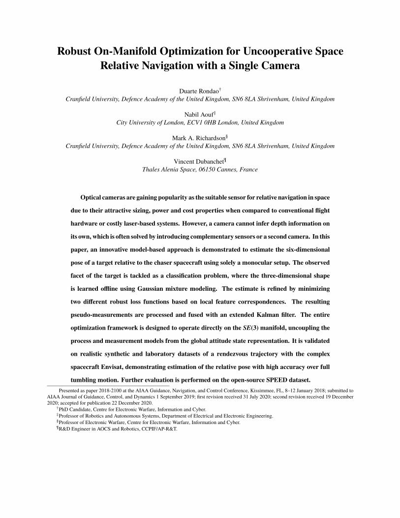
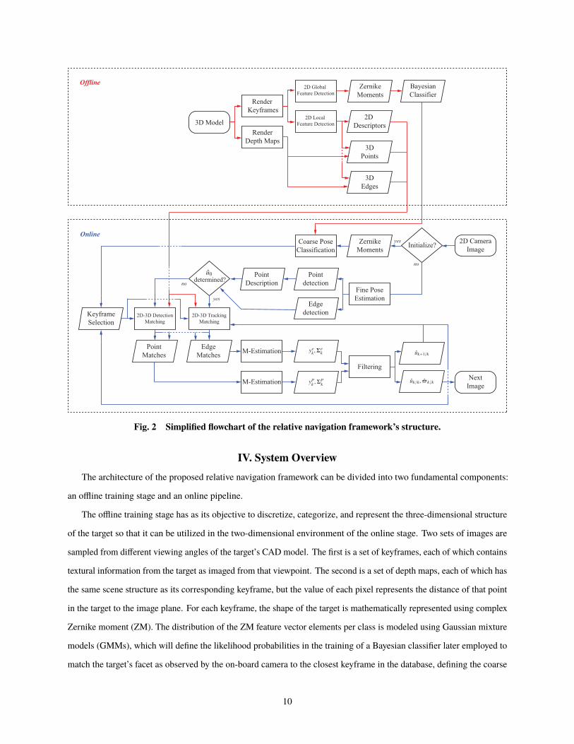
Fig. 2 Simplified flowchart of the relative navigation framework’s structure.

IV. System Overview

The architecture of the proposed relative navigation framework can be divided into two fundamental components:

an offline training stage and an online pipeline.

The offline training stage has as its objective to discretize, categorize, and represent the three-dimensional structure

of the target so that it can be utilized in the two-dimensional environment of the online stage. Two sets of images are

sampled from different viewing angles of the target’s CAD model. The first is a set of keyframes, each of which contains

textural information from the target as imaged from that viewpoint. The second is a set of depth maps, each of which has

the same scene structure as its corresponding keyframe, but the value of each pixel represents the distance of that point

in the target to the image plane. For each keyframe, the shape of the target is mathematically represented using complex

Zernike moment (ZM). The distribution of the ZM feature vector elements per class is modeled using Gaussian mixture

models (GMMs), which will define the likelihood probabilities in the training of a Bayesian classifier later employed to

match the target’s facet as observed by the on-board camera to the closest keyframe in the database, defining the coarse

10

pose classification module (Section V).

The keyframes are also processed with a feature point detector. The aim is to identify keypoints distinguishable

enough to be matched to the same keypoint in the context of the online pipeline. Each keypoint is subjected to a

feature descriptor, which generates a signature vector used to search and match in the descriptor space. Using the depth

map corresponding to its keyframe, each keypoint is annotated with its position on the target’s structure, generating

a 3D-to-2D keypoint catalog to be used with IP algorithms compatible with camera-based navigation. Additionally,

the target’s limb (or contour) in each keyframe is locally sampled into control points using edge detection. The edge

points are converted to 3D using the depth map and grouped into 3D straight keylines. It was found that existing keyline

descriptors were not mature enough for the present application, so alternative strategies were instead designed (Section

VI). The offline training stage is illustrated in red in Fig. 2.

The online stage has the purpose of providing a fine pose estimate based on local feature matching after the closest

keyframe has been found using coarse pose classification. If no estimate of the pose, D ∈ U � (�(3), has been

determined, local features are matched by detection: keypoints from the database pertaining to the current keyframe

are matched by brute-force to the ones detected in the camera image, whereas the edges are matched by aligning the

keyframe contour to the camera image contour in the least squares sense. Otherwise, the features are matched by

tracking. This is not meant in the typical sense that the features are propagated from one camera image to the next, but

instead the search space is reduced by reprojecting them from 3D into 2D based on D (Section VI.B).

The feature matches are processed separately and used to generate direct pseudo-measurements of the 6 degrees of

freedom (DOF) relative pose. This is achieved by minimizing the reprojection error using Levenberg-Marquardt (LM)

(Section VI.A) in an M-estimation framework (Section VI.D), which implements the rejection of outlying matches.

The measurements are fused with an EKF to produce an estimate of the relative pose and velocity (Section VII). Both

the M-estimator and the filter are accordant in representing the pose error as an element of se(3), meaning that the

measurement covariance determined from the former is used directly as the measurement noise in the latter, avoiding

the need for tuning. The pose predicted by the filter for the following time-step is used to select the next keyframe and in

the matching by tracking, providing temporal consistency. The online stage is summarized in blue in Fig. 2.

V. Coarse Pose Classification

A. Viewsphere Sampling

The concept of this module is to recover the viewpoint of the three-dimensional target object imaged in a two-

dimensional scene using its pre-computed and known CAD model. The objective is to provide an initial, coarse, estimate

of the appearance of the object based on its view classification so that then more precise pose estimation algorithms can

be used to refine its pose.

11

-r

rr

0

0 0

r

-r-r

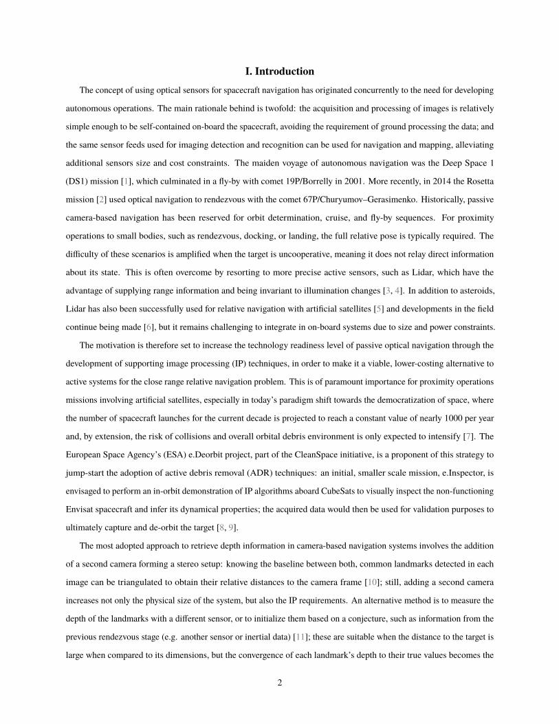
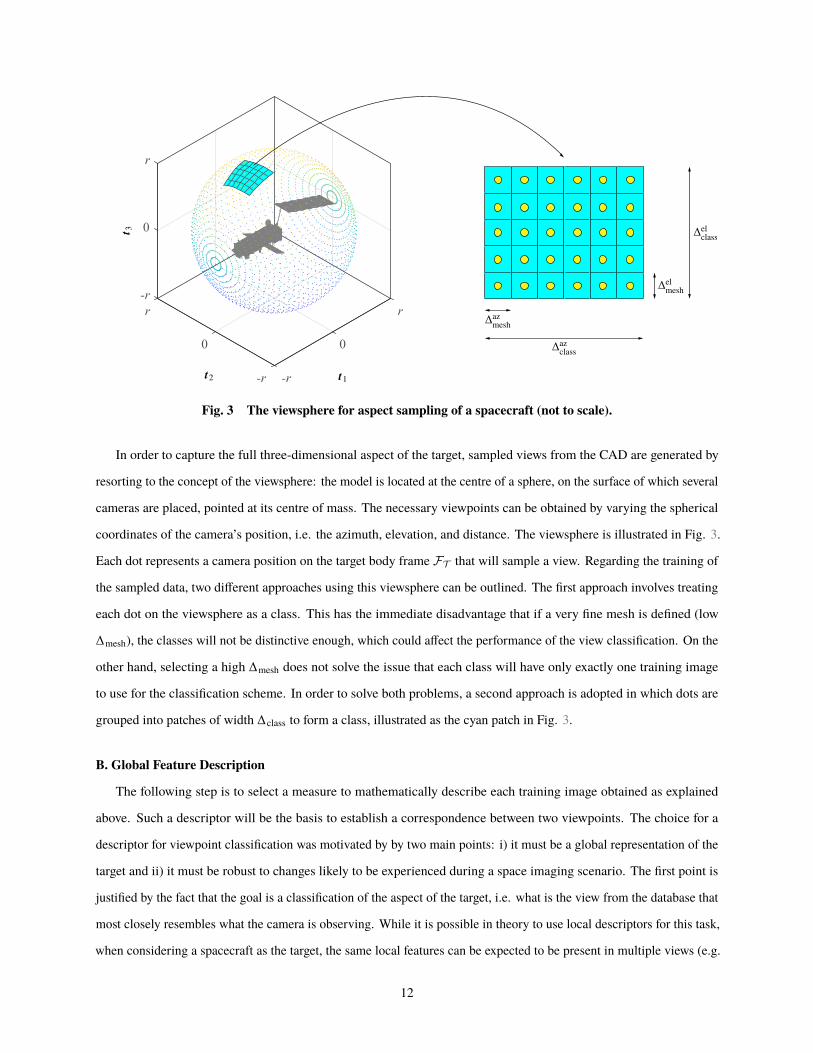
Fig. 3 The viewsphere for aspect sampling of a spacecraft (not to scale).

In order to capture the full three-dimensional aspect of the target, sampled views from the CAD are generated by

resorting to the concept of the viewsphere: the model is located at the centre of a sphere, on the surface of which several

cameras are placed, pointed at its centre of mass. The necessary viewpoints can be obtained by varying the spherical

coordinates of the camera’s position, i.e. the azimuth, elevation, and distance. The viewsphere is illustrated in Fig. 3.

Each dot represents a camera position on the target body frame FT that will sample a view. Regarding the training of

the sampled data, two different approaches using this viewsphere can be outlined. The first approach involves treating

each dot on the viewsphere as a class. This has the immediate disadvantage that if a very fine mesh is defined (low

Δmesh), the classes will not be distinctive enough, which could affect the performance of the view classification. On the

other hand, selecting a high Δmesh does not solve the issue that each class will have only exactly one training image

to use for the classification scheme. In order to solve both problems, a second approach is adopted in which dots are

grouped into patches of width Δclass to form a class, illustrated as the cyan patch in Fig. 3.

B. Global Feature Description

The following step is to select a measure to mathematically describe each training image obtained as explained

above. Such a descriptor will be the basis to establish a correspondence between two viewpoints. The choice for a

descriptor for viewpoint classification was motivated by by two main points: i) it must be a global representation of the

target and ii) it must be robust to changes likely to be experienced during a space imaging scenario. The first point is

justified by the fact that the goal is a classification of the aspect of the target, i.e. what is the view from the database that

most closely resembles what the camera is observing. While it is possible in theory to use local descriptors for this task,

when considering a spacecraft as the target, the same local features can be expected to be present in multiple views (e.g.

12

those sampled from multi-layer insulation (MLI) or solar panels), which would make the view classification harder. The

second point refers to robustness against the model and what is actually observed during the mission; since modeling all

the expected cases would be intractable, the descriptors should be resilient towards these, namely: translation, rotation,

and scale changes (i.e. the expected 6-DOF in space), off-center perspective distortions, and illumination changes.

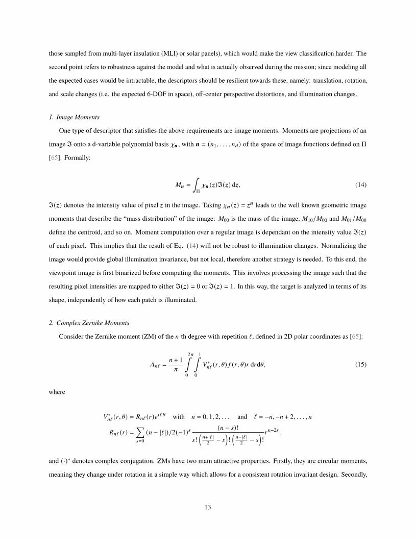
1. Image Moments

One type of descriptor that satisfies the above requirements are image moments. Moments are projections of an

image ℑ onto a d-variable polynomial basis jn, with n = (=1, . . . , =3) of the space of image functions defined on Π

[65]. Formally:

"n =

∫Π

jn (z)ℑ(z) dz, (14)

ℑ(z) denotes the intensity value of pixel z in the image. Taking jn (z) = zn leads to the well known geometric image

moments that describe the “mass distribution” of the image: "00 is the mass of the image, "10/"00 and "01/"00

define the centroid, and so on. Moment computation over a regular image is dependant on the intensity value ℑ(z)

of each pixel. This implies that the result of Eq. (14) will not be robust to illumination changes. Normalizing the

image would provide global illumination invariance, but not local, therefore another strategy is needed. To this end, the

viewpoint image is first binarized before computing the moments. This involves processing the image such that the

resulting pixel intensities are mapped to either ℑ(z) = 0 or ℑ(z) = 1. In this way, the target is analyzed in terms of its

shape, independently of how each patch is illuminated.

2. Complex Zernike Moments

Consider the Zernike moment (ZM) of the =-th degree with repetition ℓ, defined in 2D polar coordinates as [65]:

�=ℓ == + 1

c

2c∫0

1∫0

+∗=ℓ (A, \) 5 (A, \)A dAd\, (15)

where

+∗=ℓ (A, \) = '=ℓ (A)48ℓ \ with = = 0, 1, 2, . . . and ℓ = −=,−= + 2, . . . , =

'=ℓ (A) =∑B=0

(= − |ℓ |)/2(−1)B(= − B)!

B!(=+|ℓ |

2− B

)!(=−|ℓ |

2− B

)!A=−2B .

and (·)∗ denotes complex conjugation. ZMs have two main attractive properties. Firstly, they are circular moments,

meaning they change under rotation in a simple way which allows for a consistent rotation invariant design. Secondly,

13

they are orthogonal moments, which means that they present significant computational advantages with respect to

standard moments, such as low noise and uncorrelation. Additionally, orthogonal moments can be evaluated using

recurrent relations.

Since they carry these two traits, ZMs are said to be orthogonal on a disk. Hence, in order to compute the moments,

the image must be appropriately pre-processed so that it is fully contained in one. By taking this disk to be the unit disk,

scale invariance is achieved. Scale invariance is obtained when the image is mapped to the unit disk before calculation

of the moments. Translation invariance is obtained by changing the coordinate system to be centered on the centroid.

Regarding rotation invariance, one option occasionally seen is to take the ZM as the magnitude |�=ℓ |. This is not a

recommended approach, as essentially the descriptor is cut in half, leading to a likely loss in recognition power. Instead,

this work will deal explicitly with both real and complex parts of each ZM, in which case rotation invariance can be

achieved by normalizing with an appropriate, non-zero moment �<′ℓ′ (typically �31).

A fast computation of the Zernike polynomials up to a desired order can be obtained recursively since any set of

orthogonal polynomials obeys a recurrent relation for three terms; in the case of ZMs the following formula has been

developed by Kintner [66]:

:1'=+2,ℓ (A) = (:2A2 + :3)'=ℓ (A) + :4'=−2,ℓ (A), (16)

where :8 , 8 = 1, . . . , 4 are constants dependant on = and ℓ.

C. Training the Data

Given the process of generating the data and its descriptors, the final step is defining the classification method.

The classifier algorithm shall recognize the aspect of the target given a database of ZM descriptor representation

of viewpoints. Given the large volume of data involved, a Bayesian classifier is considered for this task, where the

probability density function of each class is approximated using Gaussian mixture models (GMMs).

1. Bayesian Classification

Given a specific class C<, < = 1, . . . , : , and a 3-dimensional feature vector y = (H1, . . . , H3)⊤, a Bayesian classifier

works by considering y as the realization of a random variable _ and maximizing the posterior probability % (C< |y), i.e.

the probability that the feature vector y belongs to C<. This probability can be estimated using Bayes’ formula [67]:

% (C< |y) =? (y |C<) % (C<)

:∑8=1

?(y |C8)%(C8)

. (17)

The denominator is independent from C< and hence can be simply interpreted as a scaling factor ensuring

% (C< |y) ∈ [0, 1]. Therefore, maximizing the posterior is equivalent to maximizing the numerator in Eq. (17).

14

The prior probability, % (C<), expresses the relative frequency with which C< will appear during the mission

scenario; for a general case where one has no prior knowledge of the relative motion, an equiprobable guess can be

made and the term can be set to 1/# for any <. The challenge is therefore to estimate the likelihood ?(y |C<) of class

C<, which is given by the respective probability density.

2. Gaussian Mixture Modeling

The Gaussian distribution is frequently used to model the probability density of some dataset. In the scope of the

present work, it may prove overly optimistic to assume that all elements of the ZM descriptor vectors for each class are

clustered into a single group. On the other hand, it can be too restrictive to model their distribution using hard-clustering

techniques in case boundaries are not well defined. A more controllable approach to approximate a probability density

function, while keeping the tractability of a normal distribution, is to assume the data can be modelled by a mixture of

Gaussians:

?(y |)) =

=∑8=1

U8N(y; -8 ,�8

), with N (y; -,�) =

1√(2c)3 |� |

exp

(−

1

2(y − -)) �

−1 (y − -)

), (18)

where U8 are scalar weighing factors, = is the number of mixture components, - denotes the mean vector, and � the

covariance matrix, and ) = {-1,�1, U1, . . . , -=,�=, U=} is the full set of parameters required to define the GMM.

When the number of mixture components = is known, the “optimal” mixture for each class, in the maximum

likelihood (ML) estimation sense, can be determined using the classical expectation-maximization (EM) algorithm.

EM works on the interpretation that the set of known points Y = {y1, . . . , y<} is part of a broader, complete, data set

X = Y ∪ Y that includes unknown features [67]. In the case of GMMs, or finite mixtures in general, Y = { y1, . . . , y<}

can be defined as the set of < labels denoting which component generated each sample in X . Each y8 = ( H8,1, . . . , H8,=)⊤

is a binary vector such that H8, ? = 1, H8,@ = 0 for all ? ≠ @ if sample y8 has been produced by component ?.

However, the number of components is usually not known a priori. There are several methods to iteratively estimate

the =; for this work the method of Figueiredo and Jain [68] is adopted. The algorithm provides an alternative to the

generation of several candidate models, with different numbers of mixture components, and subsequent selection of the

best fit, as this approach would still suffer from the drawbacks of EM; namely, the fact that it is highly dependant on

initialization, and the possibility of one of the mixtures’ weight U8 approaching zero (i.e. the boundary of the parameter

space) and the corresponding covariance becoming close to singular. Instead, Figueiredo and Jain’s method aims to

find the best overall model directly. This is achieved by applying the minimum message length criterion to derive the

following cost function for finite mixtures:

! () ,Y) =#

2

=∑8=1

ln(<U8

12

)+=

2ln

<

12+= (# + 1)

2− ln ? (Y; )) , (19)

15

0 10 20 30 40 50 60 70 80 90 100

Feature dimensionality

0

500

1000

1500

2000

2500

3000

3500

4000

4500

5000

No. of

GM

M p

aram

eter

s to

est

imat

eDiag. cov.

Free. cov.

(a) Necessary mixture parameters vs. 3 for = = 1

1 2

4 3

(b) Artificial transformations on training data

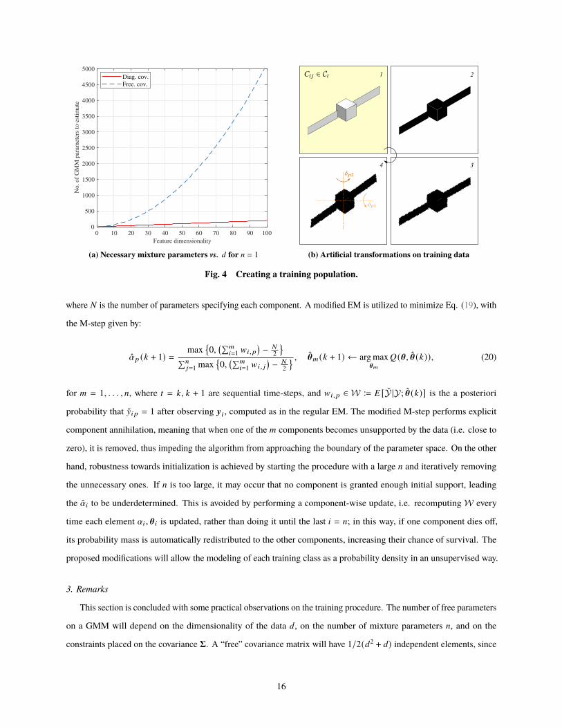
Fig. 4 Creating a training population.

where # is the number of parameters specifying each component. A modified EM is utilized to minimize Eq. (19), with

the M-step given by:

U? (: + 1) =max

{0,

(∑<8=1 F8, ?

)− #

2

}∑=

9=1 max{0,

(∑<8=1 F8, 9

)− #

2

} , )< (: + 1) ← arg max)<

&() , ) (:)), (20)

for < = 1, . . . , =, where C = :, : + 1 are sequential time-steps, and F8, ? ∈ W ≔ � [Y |Y; ) (:)] is the a posteriori

probability that H8 ? = 1 after observing y8 , computed as in the regular EM. The modified M-step performs explicit

component annihilation, meaning that when one of the < components becomes unsupported by the data (i.e. close to

zero), it is removed, thus impeding the algorithm from approaching the boundary of the parameter space. On the other

hand, robustness towards initialization is achieved by starting the procedure with a large = and iteratively removing

the unnecessary ones. If = is too large, it may occur that no component is granted enough initial support, leading

the U8 to be underdetermined. This is avoided by performing a component-wise update, i.e. recomputing W every

time each element U8 , ) 8 is updated, rather than doing it until the last 8 = =; in this way, if one component dies off,

its probability mass is automatically redistributed to the other components, increasing their chance of survival. The

proposed modifications will allow the modeling of each training class as a probability density in an unsupervised way.

3. Remarks

This section is concluded with some practical observations on the training procedure. The number of free parameters

on a GMM will depend on the dimensionality of the data 3, on the number of mixture parameters =, and on the

constraints placed on the covariance �. A “free” covariance matrix will have 1/2(32 + 3) independent elements, since

16

it is symmetric, and hence the total number of mixture parameters will be (1/232 + 3/23 + 1)= − 1. On the other hand,

the covariance can be assumed as diagonal, in which case the total number of parameters to estimate becomes 2=3 − 1.

Figure 4a plots the evolution of the number of parameters to estimate for a free covariance matrix and for a diagonal one

in terms of the dimensionality of the features for = = 1. It can be considered as a lower bound for the number of samples

< to be used in the training. The quadratic term in the free covariance case quickly diminishes the tractability of the

problem when 3 is increased, which can pose a problem when training data is limited.

In [69], it was shown that the recognition power of complex ZMs for image retrieval begins to plateau beyond

moments of the tenth order, which corresponds to approximately 3 = 60. This corresponds to 1890 parameters to

be estimated for the free covariance case, while only 120 are necessary if a diagonal covariance is assumed. Since

the ZMs are orthogonal, the correlation between moments is minimized and a diagonal covariance is an acceptable

approximation. However, even if adjacent keyframes are grouped to form classes, the generated data might not be

enough in terms of training. To this end, each keyframe �8 9 imaged for class C8 is subjected to an image augmentation

pipeline before the ZMs are computed and added to the training pool (Fig. 4b). This involves adding perturbations

to the close contour (limb) of the binarized target shape and adding small perspective distortions to the image. Data

augmentation is further explored in Section VIII.

VI. Motion Estimation

A. Problem Statement

The problem of solving the 2D-3D point correspondences for the 6-DOF pose of a calibrated camera is termed

Perspective-=-Problem (P=P) and has a well-known closed form solution for = = 3 points (P3P). It relies on the fact that

the angle between any image plane points z8 , z 9 must be the same as the angle defined between their corresponding

world points p8 , p 9 [56]. Additional methods have been developed for = ≥ 4, such as EP=P [70], which expresses the =

3D points as a weighted sum of four virtual control points and then estimates the coordinates of these control points in

the camera frame FC . While relatively fast to compute, these methods are notwithstanding less robust to noise and

fail in the presence of erroneous correspondences. On the other hand, iterative approaches that take these aspects into

account, giving the best possible estimate of the pose under certain assumptions are often called the “gold standard”

algorithm [71]. In this section, given an initial, coarse evaluation of the relative pose, an iterative refinement of its

estimate based on nonlinear manifold parameterization is proposed.

Let D represent the object to be determined. Its domain is a manifold U ⊂ R< which defines the parameter space.

Let a be the vector of measurements in R=. Suppose a is observed in the presence of noise with a covariance matrix �a,

and let a be its true value, i.e. a = a + Δa. Let h : R< → R= be a mapping such that, in the absence of noise, h(D) = a.

Varying the value of D traces out a manifold A ⊂ R= defining the set of allowable measurements, i.e. the measurement

17

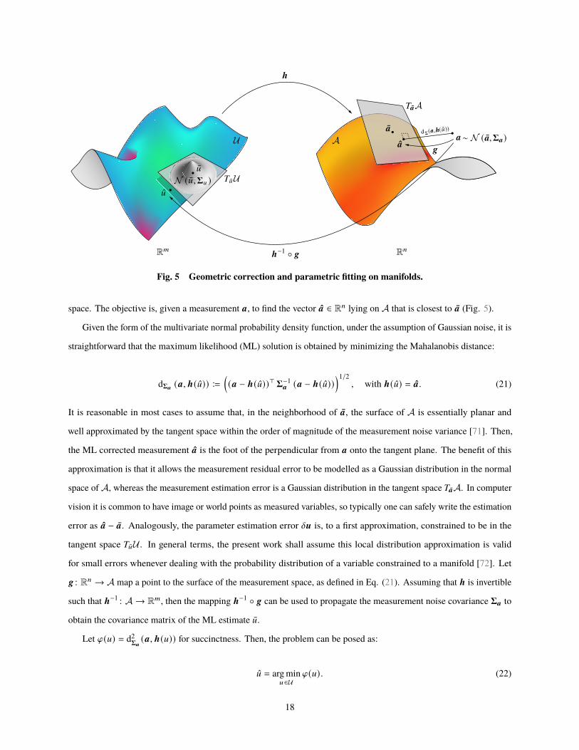
Fig. 5 Geometric correction and parametric fitting on manifolds.

space. The objective is, given a measurement a, to find the vector a ∈ R= lying on A that is closest to a (Fig. 5).

Given the form of the multivariate normal probability density function, under the assumption of Gaussian noise, it is

straightforward that the maximum likelihood (ML) solution is obtained by minimizing the Mahalanobis distance:

d�a(a, h(D)) ≔

((a − h(D))⊤ �−1

a (a − h(D)))1/2

, with h(D) = a. (21)

It is reasonable in most cases to assume that, in the neighborhood of a, the surface of A is essentially planar and

well approximated by the tangent space within the order of magnitude of the measurement noise variance [71]. Then,

the ML corrected measurement a is the foot of the perpendicular from a onto the tangent plane. The benefit of this

approximation is that it allows the measurement residual error to be modelled as a Gaussian distribution in the normal

space of A, whereas the measurement estimation error is a Gaussian distribution in the tangent space )aA. In computer

vision it is common to have image or world points as measured variables, so typically one can safely write the estimation

error as a − a. Analogously, the parameter estimation error Xu is, to a first approximation, constrained to be in the

tangent space )DU . In general terms, the present work shall assume this local distribution approximation is valid

for small errors whenever dealing with the probability distribution of a variable constrained to a manifold [72]. Let

g : R= → A map a point to the surface of the measurement space, as defined in Eq. (21). Assuming that h is invertible

such that h−1 : A→ R<, then the mapping h−1 ◦ g can be used to propagate the measurement noise covariance �a to

obtain the covariance matrix of the ML estimate D.

Let i(D) = d2�a

(a, h(D)) for succinctness. Then, the problem can be posed as:

D = arg minD∈U

i(D). (22)

18

When the function h is nonlinear, Eq. (22) may be solved iteratively by linearizing it around a reference parameter

i(D0). In the case where the parameter space U can be identified with Euclidean space, linearizing and differentiating

i(u) at u0, u ∈ R<, leads to the well-known normal equations yielding a correction Δu at iteration C = : such that

u:+1 = u: + Δu. If not, this update is not valid: as noted in Section III, u:+1 is not guaranteed to be an element of U .

One possible solution is to nevertheless apply the correction via standard addition and then project the result back to

the parameter manifold U , which could introduce additional noise in the system and drive the result away from the ML

estimate D . A more elegant alternative solution is to exploit the local Euclidean structure of U around D0 to generate a

new set of normal equations. Taking U � (�(3) and using the composition operator from Eq. (13), linearizing i(D)

yields:

i(D) ≈ i(D0) + (D ⊖ D0)⊤∇i

��D⊖D0=0

. (23)

Equation (23) thus motivates working with the pose estimation error Xu = D ⊖ D0 explicitly, which is an element of

se(3). This can be shown to lead to the normal equations of the form:

P⊤�aPXu = −P⊤�a r, (24)

where r = h(D0) − a is the residual vector. The other advantage of Eq. (24) is that the Jacobian matrix P ≔mℎ (D0⊕Xu)

m(Xu)|Xu=0

is computed with respect to the basis of se(3). At the end of each iteration, the updated parameter is obtained via the

exponential map by following Eq. (13), thus ensuring it naturally remains an element of U .

B. Structural Model Constraints

1. From Visual Point Feature Correspondences

This subsection explains how to find a relationship between some pre-existing knowledge of the target’s structure

and measurements taken of it with a digital camera that allows for the relative pose to be estimated in accordance with

the theory developed above. Note that Eq. (1) describes such a relationship, as z is the reprojection in the image plane

of a 3D point p defined in FT . Therefore, given a number of < correspondences z8 ↔ p8 between 2D image points

and 3D structural points, the task is to find Z such that z8 = 0(QZ ⊗ p8), for all 8 = 1, . . . , <. Of course, the relative

pose does not have to be represented in the homogeneous form Z; the problem is simply posited as such because of the

significance of Eq. (1) in the computer literature and, as shall be seen, because it leads to a simple form of the Jacobian.

The obvious difficulty in this formulation lies in solving the feature correspondence problem due to the topological

difference between z8 and p8 . The proposed work solves this difference by attributing to each structural point a

representation on the image plane in an offline training stage. This is achieved as follows: in each model keyframe,

point features (keypoints) are selected by a detector algorithm as centers of regions of interest (blobs) in the image.

19

These regions are typically deemed “interesting” when they have a defining property (e.g. brightness) that differs from

their surroundings. Once detected, a keypoint can then be extracted by applying a descriptor algorithm which will

encode its characterizing traits into a vector. This descriptor vector normally incorporates information about the blob

as well, allowing keypoints to be matched in different images of the same object in a robust manner with respect to

changes in scale, orientation, and brightness, among others. Since the relative pose is known for each keyframe, Eq. (1)

is inverted to generate a ray passing through each keypoint. The depth of the ray is the image of the keypoint in the

depth map corresponding to that keyframe, thus determining the equivalent 3D structural point. In this way, each p8 is

annotated offline with a 2D descriptor computed from the reprojection z′8 in the current keyframe. Then, computing

a descriptor vector for the keypoints detected online z8 grants the equivalence {z8 ↔ p8} ⇔ {z8 ↔ z′8}, reducing a

3D-2D correspondence problem to a 2D-2D one.

Since the structural points p8 are obtained via ground truth depth maps for keyframes with perfectly known Z, they

are considered to be measured with maximum accuracy, and the error is thus concentrated in the measured image points

z8 . In other words, the measurement space A is a manifold embedded in R2< (i.e. a is construed by stacking the G and

H components of all z8) and the parameter space U is 6-dimensional (i.e. the dimensions of se(3)). Furthermore, as

each measured image point is obtained algorithmically with the same feature detector, each z8 is modelled as a random

variable sampled from an isotropic (Gaussian) distribution. The ML estimate of the pose is in this manner obtained by

minimizing the geometric error (cf. Eq. (21)) which is reduced to the standard squared Euclidean distance:

Z = arg minZ ∈(�(3)

<∑8=1

d(z8 , 0

(QZ ⊗ p8

) )2. (25a)

The solution to Eq. (25a) is found iteratively via LM with the Jacobian matrix given by:

PB? =m0(Q (Z ⊕ 9) ⊗ p)

m9

����9=0

=m0′( p′)

m p′

����0′ (p′)≔0 (Qp′)p′=Z ⊗p

mZ ′ ⊗ p

mZ ′

����Z ′=Z ⊕9=Z

m exp(9)Z

m9

����9=0

=

5G?′

30 − 5G

?′1

?′23

− 5G?′

1?′

2

?′23

5G

(1 +

?′21

?′23

)− 5G

?′2

?′3

05H?′

3− 5H

?′2

?′23

− 5H

(1 +

?′22

?′23

)5H

?′1?′

2

?′23

5H?′

1

?′3

, (25b)

where 5G , 5H is the focal length and 9 ∈ se(3) is a small perturbation of the pose.

Note that the minimization scheme is built on the assumption that the structural points are known far more accurately

than the image points detected online [71]. This is a valid assumption for the context of the present study: since the CAD

model of the target is given, accurate depth maps are produced to register 3D information on the training keyframes

with virtually no error (Section IV). The actual source of error contaminating the minimization of the geometric error

consists of possible outlying matches during the online stage, which are mitigated by the M-estimation module (Section

20

VI.D). This is also the case for structural edgs (see next subsection).

2. From Visual Edge Feature Correspondences

The structural model constraints may also be formulated in terms of different types of features, such as straight line

segments. This is likewise an important element to consider in space relative navigation, as spacecraft often resemble

cuboid shapes or are composed of elements shaped as such; therefore it is expected to have detectable line features

(keylines) when imaging this kind of targets. It has been shown in this context that, while keypoints are more distinctive

in the context of minimizing Eq. (25a), keylines are actually more robust in terms of preventing the solution from

diverging [38].

In two dimensions, a point z lies on a line l = (;1, ;2, ;3)⊤ if z⊤ l = 0. Assume there exist < correspondences l 8 ↔ ℓ8

between the 2D lines and 3D lines. Therefore, one can formulate a geometric distance for 2D-3D line correspondences

in terms of the reprojection of a point p8 9 ∈ ℓ8 onto the image plane:

Z = arg minZ ∈(�(3)

<∑8=1

:∑9=0

l⊤8 QZ ⊗ p8 9 , (26)

The Jacobian matrix PB;

corresponding to the minimization of Eq. (26) can be derived in a similar manner to Eq. (25b).

In practice, matching keylines is not as straightforward as matching keypoints, as the former are typically less

distinctive than the latter. For the scope of this work, only the contour of the target is considered, which is discretized

into a finite number of edge points that are assumed to belong to a (straight) keyline. Additionally, edge points can be

registered in the same way as structural keypoints through the use of depth maps.

C. Local Feature Processing

1. Detection

Distinct point features are identified in an image of the target using the Oriented FAST and Rotated BRIEF (ORB)

detector [13]. The basis of ORB is the Features from Accelerated Segment Test (FAST) algorithm [73], developed

with the purpose of creating a high-speed keypoint finder for real-time applications†. It first selects a pixel z8 in the

image as candidate. A circle of 16 pixels around z8 and a threshold U are defined. If there exists a set of = contiguous

pixels in the circle which are all brighter than � (z8) + U or all darker than � (z8) − U, then z8 is classified as a keypoint.

The algorithm is made robust with an offline machine learning stage, training it to ignore regions in an image where it

typically lacks interest points, thus improving detection speed. As the original method is not robust to changes in size or

rotation, ORB applies a pyramidal representation of FAST for multi-scale feature detection and assigns an orientation

to each one by defining a vector from its origin to the intensity baricenter of its support region. The choice for the

†Although ORB has also been developed for feature description, using a modification of the Binary Robust Invariant Scalable Keypoints (BRIEF)

algorithm, it is applied herein for detection only.

21

keypoint algorithms (see also Section VI.C.2) is the product of the authors’ previous survey on IP techniques for relative

navigation in space [74].

The Canny algorithm is the basis for edge detection [75]. First, the image is filtered with a Gaussian kernel in order

to remove noise. Secondly, the intensity gradients at each pixel are computed. Then, non-maximal suppression and a

double thresholding are applied to discard spurious responses and identify edge candidates. The method from Ref. [76]

is used to efficiently extract keylines from the edge image by incrementally connecting edge pixels in straight lines and

merging those with small enough differences in overlap and orientation.

2. Description

For each detected keypoint, a binary string is generated encoding information about its support region using the Fast

Retina Keypoint (FREAK) descriptor [77], which takes inspiration in the design of the human retina. The method adopts

the retinal sampling grid as the sampling pattern for pixel intensity comparisons, i.e. a circular design with decreasing

density from the center outwards, achieved using different kernel sizes for the Gaussian smoothing of every sample

point in each receptive field; these overlap for added redundancy leading to increased discriminating power. Each bit in

the descriptor thus represents the result of each comparison test, which only has two possible outcomes: either the

first pixel is brighter than the second, or vice-versa. A coarse-to-fine pair selection is employed to maximize variance

and uncorrelation between pairs. In this way, the first 16 bytes of the descriptor represent coarse information, which is

applied as a triage in the matching process, and a cascade of comparisons is performed to accelerate the procedure even

further.

3. Brute-Force Detection Matching

In an initial stage, the features are matched using brute force, since no estimate of the pose is yet available. In the

case of the point features, this implies that all those detected in the initial frame are compared against those in the train

keyframe. This is achieved by computing the Hamming distance dHam (·, ·) between their corresponding descriptors, i.e.

the minimum number of substitutions required to convert one into the other. It can be swiftly computed by applying

the exclusive-OR (XOR) operator followed by a bit count, which provides an advantage in terms of computational

performance with respect to the Euclidean distance test used with more traditional floating point descriptors. For each

query, the two closest train descriptor matches are selected and subjected to a nearest-neighbour distance ratio (NNDR)

test: the matching of the descriptors s8 and s 9 is accepted if

dHam (s8 , s 9 )

dHam (s8 , s: )< `NNDR, (27)

where s 9 , s: are the 1st and 2nd nearest neighbours to s8 and `NNDR is a ratio from 0 to 1.

22

As descriptors for edge features are not employed, an alternative strategy was devised to match them. The full

contours D@ ,DC ⊂ R2 of the target in the query image and the train keyframe, respectively, are considered. Each

contour is a set of = discretized edge points of the same size, i.e. D@ = {z@,1, . . . , z@,=} and DC = {zC ,1, . . . , zC ,=}. Even

though the query image and train keyframe represent the same aspect of the target, there will be differences that are

reflected on the contours. In particular, D@ and DC will be different by a 2D affine transformation Λ(V, \, t) : DC → D@ ,

where V > 0 is a scaling factor, \ ∈ [−c, c[ rad is an angle of rotation and t = (C1, C2)⊤ is a translation vector. The

contour alignment problem is posed in the least squares sense as

arg mint ,V, \

dFro

(D@ ,Λ (DC )

), (28)

where dFro (·, ·) is the Frobenius distance. Because of the multiplicative trigonometric terms of Λ, Eq. (28) is nonlinear.

However, the problem can be converted into an equivalent linear one by a change of variables [78]:

arg min(C1 ,C2 ,11 ,12) ∈R4

d

©­­­­­­«

©­­­­­­«

I@,1,1I@,1,2...

I@,=,1I@,=,2

ª®®®®®®¬,

1 0 IC ,1,1 −IC ,1,20 1 IC ,1,2 IC ,1,1...

......

...

1 0 IC ,=,1 −IC ,=,20 1 IC ,=,2 IC ,=,1

©­­­«

C1C211

12

ª®®®¬

ª®®®®®®¬with

(11

12

)= V

(cos \

sin \

)⇔

(\

V

)=

©­­«arcsin

(12/

√12

1+ 12

2

)√12

1+ 12

2

ª®®¬,

(29)

where zD,E = (ID,E,1, ID,E,2)⊤. In this way, a global solution of the minimum can be calculated using standard linear

algebra. However, Eq. (29) depends on the correspondences between the query and train edge points, which are

not known a priori. To simultaneously solve for the edge point correspondence problem and contour alignment, the

algorithm is modified by solving = linear least squares problems, each time shifting the order of the edge points in DC by

one, and selecting the minimum of the = residual norms. Thus, the only necessary inputs are two sets of sequential but

not necessarily correspondent edge points.

4. Predictive Tracking Matching

Once the algorithm is initialized, knowledge of the current solution can be used to improve the performance of the

feature matching processes. In particular, the predicted estimate of the pose output by the filtering module is used to

help anticipate where the features will be located in the next frame in time, in this way introducing a temporal tracking

constraint that improves the pose estimation accuracy.

In the case of point features, tracking matching is achieved by fitting a grid of ? × @ cells on the boundary of the

target in the query camera image. The detected keypoins are binned into the resulting cells. Then, the 3D structural

points of the currently selected database keyframe are reprojected onto the query image according to the predicted pose

(cf. Eq. (1)) and equally binned according to the grid. Lastly, descriptor-based matching is applied on a per-cell basis,

23

(a) 0% outliers (b) 25% outliers (c) 50% outliers

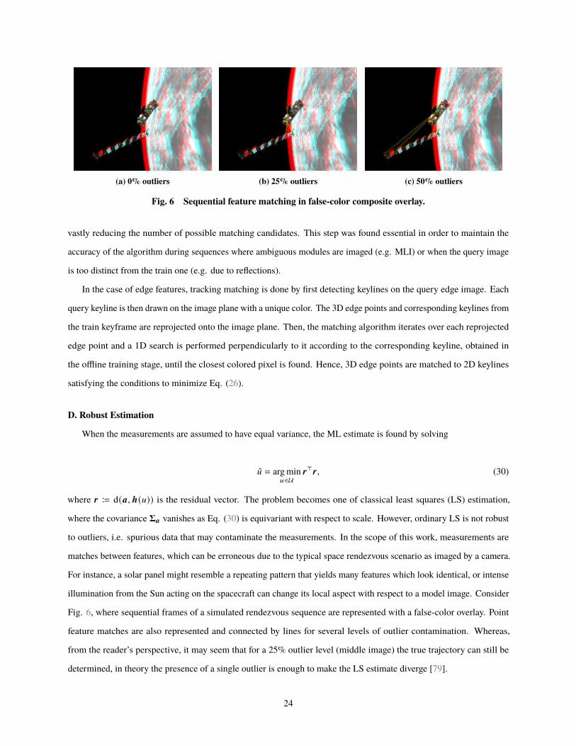
Fig. 6 Sequential feature matching in false-color composite overlay.

vastly reducing the number of possible matching candidates. This step was found essential in order to maintain the

accuracy of the algorithm during sequences where ambiguous modules are imaged (e.g. MLI) or when the query image

is too distinct from the train one (e.g. due to reflections).

In the case of edge features, tracking matching is done by first detecting keylines on the query edge image. Each

query keyline is then drawn on the image plane with a unique color. The 3D edge points and corresponding keylines from

the train keyframe are reprojected onto the image plane. Then, the matching algorithm iterates over each reprojected

edge point and a 1D search is performed perpendicularly to it according to the corresponding keyline, obtained in

the offline training stage, until the closest colored pixel is found. Hence, 3D edge points are matched to 2D keylines

satisfying the conditions to minimize Eq. (26).

D. Robust Estimation

When the measurements are assumed to have equal variance, the ML estimate is found by solving

D = arg minD∈U

r⊤r, (30)

where r ≔ d(a, h(D)) is the residual vector. The problem becomes one of classical least squares (LS) estimation,

where the covariance �a vanishes as Eq. (30) is equivariant with respect to scale. However, ordinary LS is not robust

to outliers, i.e. spurious data that may contaminate the measurements. In the scope of this work, measurements are

matches between features, which can be erroneous due to the typical space rendezvous scenario as imaged by a camera.

For instance, a solar panel might resemble a repeating pattern that yields many features which look identical, or intense

illumination from the Sun acting on the spacecraft can change its local aspect with respect to a model image. Consider

Fig. 6, where sequential frames of a simulated rendezvous sequence are represented with a false-color overlay. Point

feature matches are also represented and connected by lines for several levels of outlier contamination. Whereas,

from the reader’s perspective, it may seem that for a 25% outlier level (middle image) the true trajectory can still be

determined, in theory the presence of a single outlier is enough to make the LS estimate diverge [79].

24

Robustness with respect to outliers can be achieved by generalizing Eq. (30) into an M-estimator:

D = arg minD∈U

#∑8=1

d( A8f

), (31)

where d is a symmetric, positive-definite function with subquadratic growth, and f2 is an estimate of the variance, or

scale, of r. Solving Eq. (31) implies#∑8=1

k( A8f

) dA8

dD

1

f= 0, (32)

where k(G) ≔ dd(G)/dG is defined as the influence function of the M-estimator. This function measures the influence

that a data point has on the estimation of the parameter D. A robust M-estimator d(G) should meet two constraints:

convexity in G, and a bounded influence function [80]. By acknowledging the latter point, it becomes clear why the

general LS is not robust, since d(G) = G2/2 and therefore k(G) = G.

There are two possible approaches to define the normal equations for M-estimation that avoid the computation of the

Hessian [81]:

P⊤PXu = −P⊤7( rf

)f, (33a)

P⊤]PXu = −P⊤]r, (33b)

where ] = diag(F(A1/f), . . . , F(A=/f)) and F(G) ≔ k(G)/G. The first method was developed by Huber [82] and

generalizes the normal equations through the modification of the residuals via k and f. Huber proposed a specific loss

function, the Huber M-estimator dHub (G). Huber’s algorithm provides a way to jointly estimate the scale f alongside

the parameter D with proven convergence properties. The minimization algorithm (e.g. LM) is simply appended with

the procedure:

f2:+1 =

1

(= − ?)V

=∑8

(A8

f:

)2

f2: , (34)

where V is a bias-correcting factor. The second method was developed by Beaton and Tukey [83] and is commonly

known as iteratively reweighed least squares (IRLS), due to the inclusion of the weights matrix ] that assumes the role

of �a (cf. Eq. (24)). Tukey proposed an alternative robust loss function, dTuk (G).

Each robust loss function, dHub (G) and dTuk(G), can be compared regardless of the formulation. The Huber

M-estimator is considered to be adequate for almost all situations, but does not eliminate completely the influence of

large errors [80]. On the other hand, the Tukey M-estimator is non-convex, but is a “hard redescender”, meaning that its

influence function tends to zero quickly so as to aggressively reject outliers, explaining its frequent use in computer

vision applications, where the outliers typically have small residual magnitudes [84].

25

0 3 6 9 12 15

Iteration number

0

0.2

0.4

0.6

0.8

1

1.2

Norm

ali

zed t

ransl

ati

on e

rror

(-)

0 3 6 9 12 15

Iteration number

0

0.2

0.4

0.6

Norm

ali

zed a

ttit

ude e

rror

(-)

(a) 10% outliers

0 3 6 9 12 15

Iteration number

0

5

10

15

20

25

Sca

le (

px)

0 3 6 9 12 15

Iteration number

0

0.2

0.4

0.6

0.8

1

1.2

Norm

ali

zed t

ransl

ati

on e

rror

(-)

0 3 6 9 12 15

Iteration number

0

0.2

0.4

0.6

Norm

ali

zed a

ttit

ude e

rror

(-)

(b) 20% outliers

0 3 6 9 12 15

Iteration number

0

5

10

15

20

25

Sca

le (

px)

0 3 6 9 12 15

Iteration number

0

0.2

0.4

0.6

0.8

1

1.2

Norm

ali

zed t

ransl

ati

on e

rror

(-)

0 3 6 9 12 15

Iteration number

0

0.2

0.4

0.6

Norm

ali

zed a

ttit

ude e

rror

(-)

(c) 30% outliers

0 3 6 9 12 15

Iteration number

0

5

10

15

20

25

Sca

le (

px)

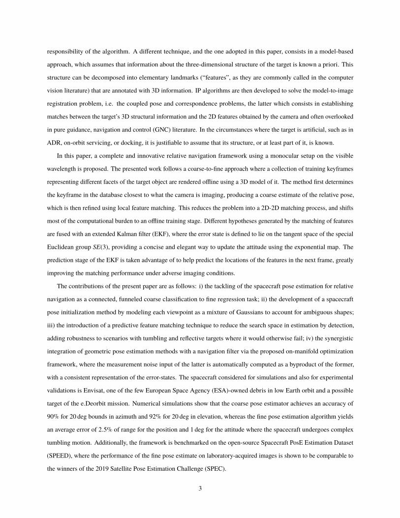
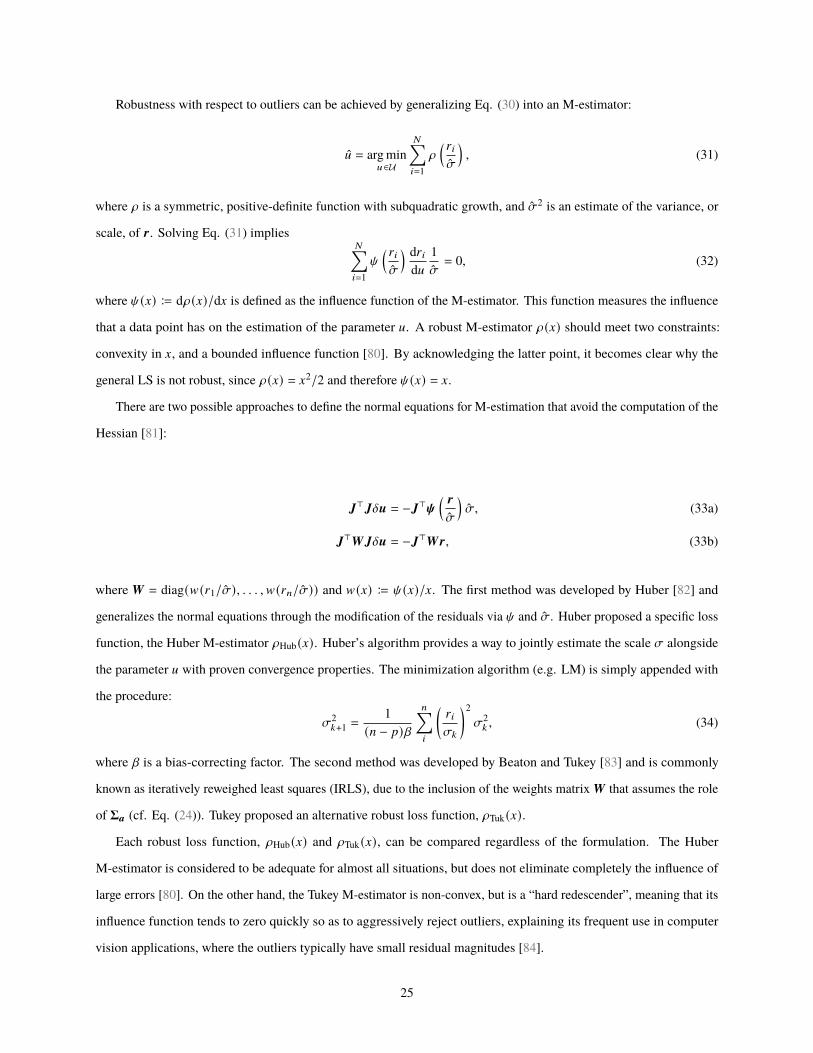
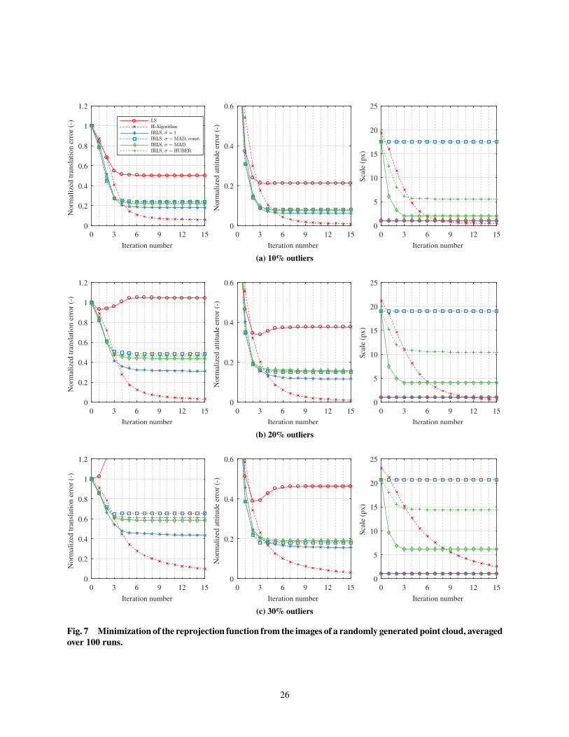
Fig. 7 Minimization of the reprojection function from the images of a randomly generated point cloud, averaged

over 100 runs.

26

The scale estimation step warrants special attention. In several applications, it can be found that f is often ignored

and set to 1. This is erroneous since Eq. (31) is non-equivariant with respect to scale [79]. Whereas the Huber algorithm

(Eq. (33a)) grants a procedure to jointly estimate the parameter and scale, convergence is not guaranteed when applying

the scale estimation step to IRLS (Eq. (33b)) [85]. Instead, a common method when resorting to IRLS is to recursively

estimate f using the median absolute deviation (MAD) for the first few iterations, and then allowing the minimization

to converge on D with fixed f [80, 84].

In order to study the effect of scale estimation on the parameter estimation and to compare the different possible

approaches, an experiment has been devised. First, a number of 3D world points is randomly sampled from the volume

of a cube. They are subsequently projected onto the image plane according to a random pose. Points that fall outside the

image plane are culled. Matches between 3D world points and 2D camera points are contaminated artificially with

outliers. Then, the pose is M-estimated with dHub (G) according to the cost function of Eq. (25a), where the initial

guess is defined by contaminating the true pose with zero-mean, white, Gaussian noise. Five distinct methods are

benchmarked: i) LS, ii) Huber’s algorithm, iii) IRLS with f = 1, iv) IRLS with f estimated by one iteration of MAD,

v) IRLS with f estimated by three iterations of MAD, vi) IRLS with f estimated by Huber’s algorithm. The experiment

is repeated for several trials.

The results are shown in Fig. 7. The pose estimation error is decomposed into translation and rotation normalized

according to the initial guess. The evolution of the scale estimation is also shown. The percentage of outliers present in

the data ranges from 10% to 30%. It can be seen that Huber’s algorithm yields the best estimate for every case. The

regular LS is able to somewhat reduce the attitude error in the presence of outliers, but diverges in the case of translation.

Interestingly, all the IRLS methods that estimate the scale perform worse than the case where the scale is ignored. These

results show the impact on the solution of proper scale estimation and the preference of Huber’s algorithm over others.

This suggests that robust estimation should be initiated with Huber’s algorithm until convergence; to ensure that the

rejection of outliers is maximized, some additional iterations can be performed with IRLS and a hard redescender, such

as Tukey’s function, using the (fixed) previously obtained estimate of f, as suggested in Ref. [80].

VII. Filtering

A. Rigid Body Kinematics

The kinematics equation for (�(3) in matrix form is [57]:

¤Z�/) = ;�∧�/)Z�/) , with ;�

�/) ≔

(.��/)

8��/)

), (35)

where Z�/) is the rigid body pose mapping FT to FB, and ;��/)

is the rigid body velocity of FT with respect to FB

expressed in FB. It is the concatenation of two terms: 8, the instantaneous angular velocity of the target as seen from

27

the chaser; and ., the velocity of the point in FT that corresponds instantaneously to the origin of FB. Dropping the

subscripts and superscripts for succinctness, Eq. (35) is a first-order ordinary differential equation, and hence admits a

closed-form solution of the form:

Z (C) = exp((C − C0);∧)Z (C0). (36)

Equation (36) has the same form as Eq. (9), implying that ; is an element of se(3). In agreement with the previous

sections, this fact suggests that uncertainty can be introduced in the pose kinematics by modeling it as a local distribution

in se(3). As such, it is of interest to develop perturbation equations in terms of the kinematics in se(3) so that these can

be included as additive noise in a filtering scheme.

Following the approach of Ref. [86], the first two terms of Eq. (3) are used to linearize Eq. (9) as Z ′ ≈ (O + X/∧)Z,

where Z is the nominal pose, X/ is a small perturbation in se(3), and hence Z ′ is the resulting perturbed pose. Since

; ∈ se(3), this generalized velocity can be written directly as the sum of a nominal term with a small perturbation

;′ = ; + X;. Substituting in Eq. (35), one has:

d

dC

( (O + X/∧

)Z)≈ (; + X;)∧

(O + X/∧

)Z. (37)

Expanding, ignoring the product of small terms and applying the Lie bracket of se(3) yields the perturbation kinematics

equation for (�(3):

X ¤/ = ad(;)X/ + X;, (38)

which is linear in both X/ and X;.

B. Extended Kalman Filter Formulation

1. Motion Model

Equation (38) describes effectively the linearization of the rigid body kinematics around a nominal pose. Since it is

defined with respect to elements of se(3), perturbations in the motion can be modelled stochastically in terms of a local

distribution (Section VI). The mean of this distribution may be injected into the nominal values via the exponential

map. Under the assumption of Gaussian noise, this equation can therefore be regarded as the first step in defining an

error-state to model how the motion evolves in time in the framework of an extended Kalman filter.

The kinematics of the target’s motion with respect to the chaser spacecraft are correctly modelled by Eqs. (35)

and (38). Modelling the relative dynamics, however, is not a clear-cut task. In the case of an asteroid mission, for

example, the chaser could be considered to be inside the sphere of influence of the target and then Newton’s second law

of motion and Euler’s rotation equation could be applied. However, in the case where both chaser and target are under

28

the influence of the same primary, the relative dynamics cannot be shaped as such.

In order to design a filter exclusively with relative states, and inspired by the method of Ref. [87], a broader constant

generalized velocity motion model is adopted:

¤;(C) = (; (C), (; (C) ∼ N (0,W(C)X(C − g)), (39)

where it is assumed that the spectral density matrix W(C) is diagonal. Note that, as stated in Ref. [87], this model

does not assume that the chaser moves at a constant velocity over the entire sequence, but instead that undetermined

accelerations with a Gaussian profile are expected to occur on average. In other words, one assumes that sizeable

(relative) accelerations are unlikely to be experienced, which is a valid expectation for a space rendezvous.

Integrating Eq. (39) yields ;(C) = ;(C0) +∫ C

C0(; (g) dg. The relation ;′ = ; + X; was assumed earlier, meaning

that one can admit

X;(C) =

C∫C0

(; (g) dg. (40)

Defining the error state Xx ≔ (X/, X;)⊤, the continuous-time error kinematics are written directly:

d

dCXx(C) = L(C)Xx(C) + M (C)w(C) =

[ad(;) O6

06×6 06×6

] (X/

X;

)+

[06×6

O6

] (03×1

(;

), (41)

which shows that process noise is introduced in the system through the error generalized velocity vector. Equation (41)

has the familiar solution [88]:

Xx(C) = exp©­«

C∫C0

L(g)dgª®¬Xx(C0) +

C∫C0

exp©­«

C∫B

L(g)dgª®¬M (B)w(B)dB (42)

The error-state transition matrix has a known closed form [86]:

�(C, B) ≔ exp©­«

C∫B

L(g)dgª®¬=

[Ad(exp((C − B);∧)) (C − B)H((C − B);))

03×3 O3

], with H(/) ≔

[S (5) T(/)

03×3 S (5)

],

(43)

where, defining q ≔ ‖5‖,

S (/) ≔1

21∧ +

(q − sin q

q3

) (5∧1∧ + 1∧5∧ + 5∧1∧5∧

)+

(q2 + 2 cos q − 2

2q4

) (5∧5∧1∧ + 1∧5∧5∧ − 35∧1∧5∧

)+

(2q − 3 sin q + q cos q

2q5

) (5∧1∧5∧5∧ + 5∧5∧1∧5∧

).

(44)

29

A closed-form of the discrete-time error process noise covariance matrix is found by directly solving the integral:

�(C, B) ≔

C∫C0

�(C, B)M (B)W(B)M⊤ (B)�⊤ (C, B) dB, (45)

The derivation is monotonous but a matter of integrating each matrix element. To simplify it, the small angle

approximation is applied and terms of O((C − B)4) are discarded; the final result is not presented here.

2. Measurement Model

The correction stage of the EKF admits pseudo-measurements of the relative pose H8 ∈ Y � (�(3) as obtained

through the refinement scheme of visual features correspondence from Section VI. These pseudo-measurements are

acquired at each sampling time and modelled as being corrupted by a zero-mean white Gaussian noise term. One can

thus write directly in discrete-time and matrix form:

_ = exp((∧H )Z, (H ∼ N (0, X), (46)

where _ ∈ (�(3) is the matrix form of H. To linearize Eq. (46), similarly to the motion model, the elements of (�(3)

are rewritten as a small perturbation around a nominal term, i.e. _ ′ = exp(Xy∧)_ , Z ′ = exp(X/∧)Z, and the exponential

map is approximated by its first-order expression. Replacing in Eq. (46), expanding and neglecting the product of small

terms, the following linearized relationship is obtained:

_ ′= Z ′, Xy = X/ + (H . (47)

The full linearized measurement model is therefore:

Xy8 = NXx + (H8=

[O6 06×6

] (X/

X;

)+ (H8

, (H8∼ N (0, X8) (48)

The covariance matrices of each pseudo-measurement are obtained as a product of the minimization scheme. In the

case of the structural model constraints, the Jacobians PB are of rank 6, so the covariance of the solution is given by

backpropagation of the visual feature correspondences’ own covariance [71]:

XB = �B =(P⊤B �z,s PB

)−1, (49a)

with �z,s = f2z,s O and fz,s is obtained via M-estimation (cf. Subsection VI.D). The EKF innovation term at C = : is:

4B,: = HB,: ⊖ D−: ∈ se(3), (49b)

30

where D−:

is the predicted pose at C = : .

3. Measurement Gating

An additional step is employed prior to the correction to ensure the accurate functioning of the filter. This involves

subjecting the incoming measurements to a validation gate, thus discarding potential spurious data. The validation gate

is a threshold on the root mean square error (RMSE) of the residuals r as obtained by the M-estimation:

RMSE(r) ≔

√∑=8=1 A

28

=. (50)

The RMSE provides an objective and clear interpretation of how close, in pixels, does the feature matching agree with

the estimate of the pose.

C. Manifold State Prediction and Correction

The nominal state is construed as x⊤ = (D⊤,;⊤), with D ∈ U � (�(3) representing the relative pose mapping

FT → FB and ; ∈ R6 is the generalized velocity satisfying the kinematics equation for (�(3), Eq. (35). The nominal

state estimate is updated with a linearized error state estimate Xx⊤ = (X/⊤, X;⊤) ∈ se(3) × R6 via pose composition

(cf. Eq. (13)), ensuring that D remains an element of U � (�(3). The algorithm’s equations are valid for any chosen

representation of D provided the appropriate composition ⊕ is used. State prediction is performed as:

D−: = D:−1 ⊕ ΔC;:−1, ;−: = ;:−1. (51)

The state correction is given by:

D+: = D−: ⊕ X/+

: , ;+: = ;−: + X;+: , (52)

where Xx−⊤:

= (D−⊤:

, ;−⊤: ), Xx+⊤:

= (D+⊤:, ;+⊤: ) are the a priori and a posteriori error states, respectively. The covariance

is calculated using the standard EKF equations.

In terms of the parameterization of D, a possible choice would be taking D → Z directly, in which case the composition

operation is given by Eq. (9). Alternatively, the unit quaternion is a popular choice for attitude parameterization

due to its compact and singularity-free representation, particularly in aerospace applications. The exponential map

so(3)→ (*(2) has a simple closed form given by exp@ = (5⊤ sin(q/2)/q, cos q/2)⊤, with q = ‖5‖. [89]. In this case,

the state vector becomes, with some abuse of notation, x⊤ = (D⊤,;⊤) = ( t⊤, q⊤,;⊤), which has dimension 13 × 1.

31

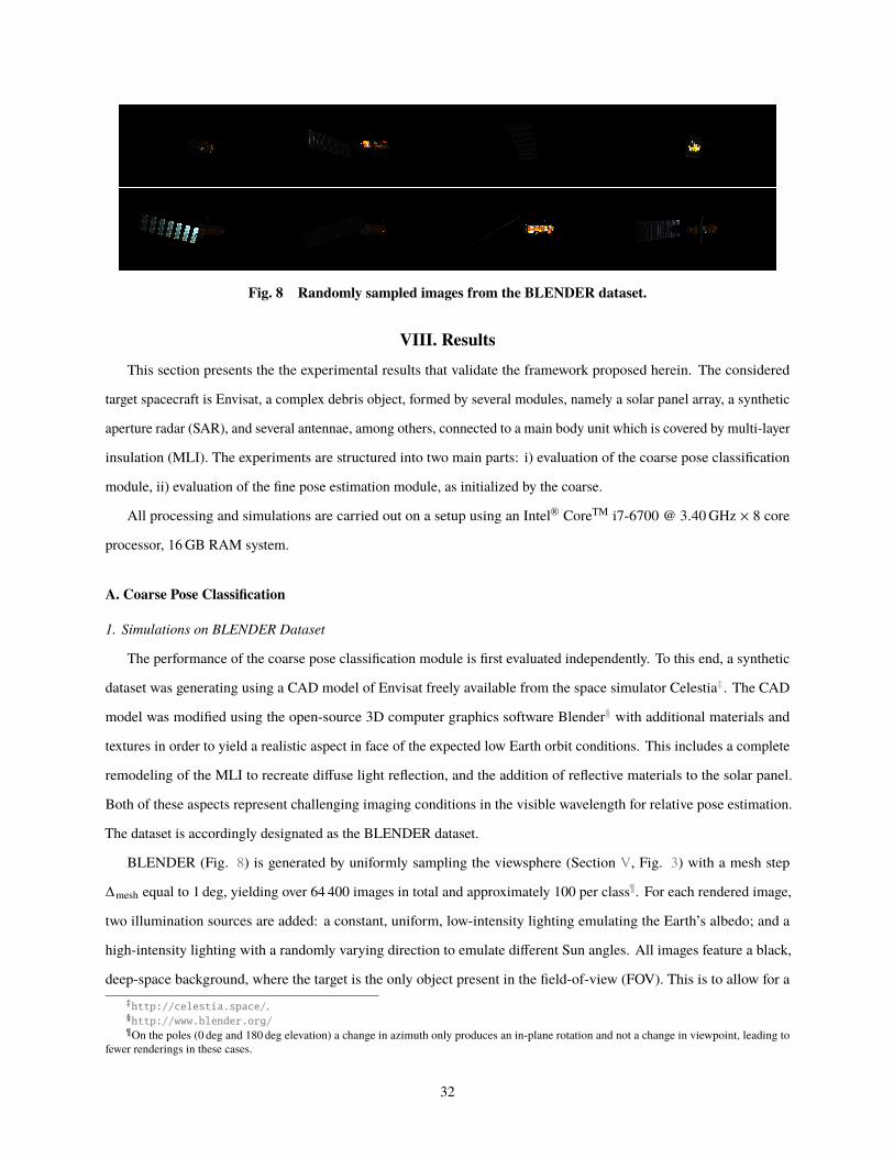
Fig. 8 Randomly sampled images from the BLENDER dataset.

VIII. Results

This section presents the the experimental results that validate the framework proposed herein. The considered

target spacecraft is Envisat, a complex debris object, formed by several modules, namely a solar panel array, a synthetic

aperture radar (SAR), and several antennae, among others, connected to a main body unit which is covered by multi-layer

insulation (MLI). The experiments are structured into two main parts: i) evaluation of the coarse pose classification

module, ii) evaluation of the fine pose estimation module, as initialized by the coarse.

All processing and simulations are carried out on a setup using an Intel® CoreTM i7-6700 @ 3.40 GHz × 8 core

processor, 16 GB RAM system.

A. Coarse Pose Classification

1. Simulations on BLENDER Dataset

The performance of the coarse pose classification module is first evaluated independently. To this end, a synthetic

dataset was generating using a CAD model of Envisat freely available from the space simulator Celestia‡. The CAD

model was modified using the open-source 3D computer graphics software Blender§ with additional materials and

textures in order to yield a realistic aspect in face of the expected low Earth orbit conditions. This includes a complete

remodeling of the MLI to recreate diffuse light reflection, and the addition of reflective materials to the solar panel.

Both of these aspects represent challenging imaging conditions in the visible wavelength for relative pose estimation.

The dataset is accordingly designated as the BLENDER dataset.

BLENDER (Fig. 8) is generated by uniformly sampling the viewsphere (Section V, Fig. 3) with a mesh step

Δmesh equal to 1 deg, yielding over 64 400 images in total and approximately 100 per class¶. For each rendered image,

two illumination sources are added: a constant, uniform, low-intensity lighting emulating the Earth’s albedo; and a

high-intensity lighting with a randomly varying direction to emulate different Sun angles. All images feature a black,

deep-space background, where the target is the only object present in the field-of-view (FOV). This is to allow for a

‡http://celestia.space/.§http://www.blender.org/¶On the poles (0 deg and 180 deg elevation) a change in azimuth only produces an in-plane rotation and not a change in viewpoint, leading to

fewer renderings in these cases.

32

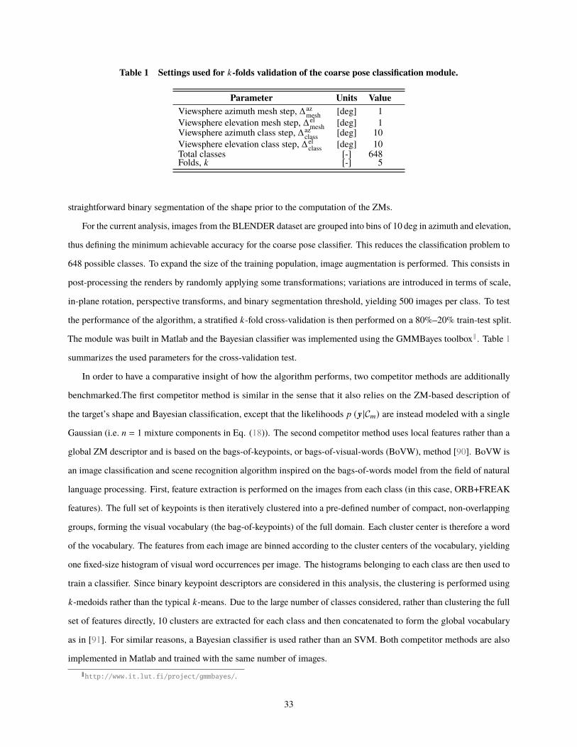
Table 1 Settings used for :-folds validation of the coarse pose classification module.

Parameter Units Value

Viewsphere azimuth mesh step, Δazmesh

[deg] 1

Viewsphere elevation mesh step, Δelmesh

[deg] 1Viewsphere azimuth class step, Δaz

class[deg] 10

Viewsphere elevation class step, Δelclass

[deg] 10Total classes [-] 648Folds, : [-] 5

straightforward binary segmentation of the shape prior to the computation of the ZMs.

For the current analysis, images from the BLENDER dataset are grouped into bins of 10 deg in azimuth and elevation,

thus defining the minimum achievable accuracy for the coarse pose classifier. This reduces the classification problem to

648 possible classes. To expand the size of the training population, image augmentation is performed. This consists in

post-processing the renders by randomly applying some transformations; variations are introduced in terms of scale,

in-plane rotation, perspective transforms, and binary segmentation threshold, yielding 500 images per class. To test

the performance of the algorithm, a stratified :-fold cross-validation is then performed on a 80%–20% train-test split.

The module was built in Matlab and the Bayesian classifier was implemented using the GMMBayes toolbox‖. Table 1

summarizes the used parameters for the cross-validation test.

In order to have a comparative insight of how the algorithm performs, two competitor methods are additionally

benchmarked.The first competitor method is similar in the sense that it also relies on the ZM-based description of

the target’s shape and Bayesian classification, except that the likelihoods ? (y |C<) are instead modeled with a single

Gaussian (i.e. = = 1 mixture components in Eq. (18)). The second competitor method uses local features rather than a

global ZM descriptor and is based on the bags-of-keypoints, or bags-of-visual-words (BoVW), method [90]. BoVW is

an image classification and scene recognition algorithm inspired on the bags-of-words model from the field of natural

language processing. First, feature extraction is performed on the images from each class (in this case, ORB+FREAK

features). The full set of keypoints is then iteratively clustered into a pre-defined number of compact, non-overlapping

groups, forming the visual vocabulary (the bag-of-keypoints) of the full domain. Each cluster center is therefore a word

of the vocabulary. The features from each image are binned according to the cluster centers of the vocabulary, yielding

one fixed-size histogram of visual word occurrences per image. The histograms belonging to each class are then used to

train a classifier. Since binary keypoint descriptors are considered in this analysis, the clustering is performed using

:-medoids rather than the typical :-means. Due to the large number of classes considered, rather than clustering the full

set of features directly, 10 clusters are extracted for each class and then concatenated to form the global vocabulary

as in [91]. For similar reasons, a Bayesian classifier is used rather than an SVM. Both competitor methods are also

implemented in Matlab and trained with the same number of images.

‖http://www.it.lut.fi/project/gmmbayes/.

33

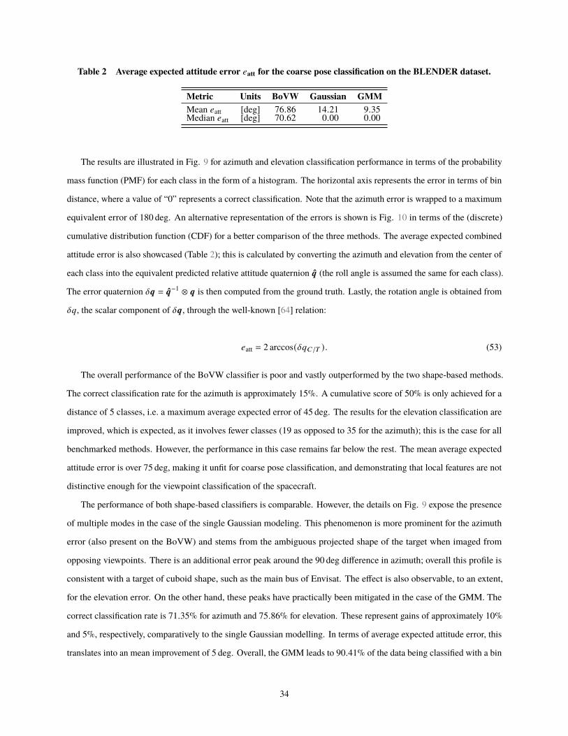
Table 2 Average expected attitude error 4att for the coarse pose classification on the BLENDER dataset.

Metric Units BoVW Gaussian GMM

Mean 4att [deg] 76.86 14.21 9.35Median 4att [deg] 70.62 0.00 0.00

The results are illustrated in Fig. 9 for azimuth and elevation classification performance in terms of the probability

mass function (PMF) for each class in the form of a histogram. The horizontal axis represents the error in terms of bin

distance, where a value of “0” represents a correct classification. Note that the azimuth error is wrapped to a maximum

equivalent error of 180 deg. An alternative representation of the errors is shown is Fig. 10 in terms of the (discrete)

cumulative distribution function (CDF) for a better comparison of the three methods. The average expected combined

attitude error is also showcased (Table 2); this is calculated by converting the azimuth and elevation from the center of

each class into the equivalent predicted relative attitude quaternion q (the roll angle is assumed the same for each class).

The error quaternion Xq = q−1 ⊗ q is then computed from the ground truth. Lastly, the rotation angle is obtained from

X@, the scalar component of Xq, through the well-known [64] relation:

4att = 2 arccos(X@�/) ). (53)

The overall performance of the BoVW classifier is poor and vastly outperformed by the two shape-based methods.

The correct classification rate for the azimuth is approximately 15%. A cumulative score of 50% is only achieved for a

distance of 5 classes, i.e. a maximum average expected error of 45 deg. The results for the elevation classification are

improved, which is expected, as it involves fewer classes (19 as opposed to 35 for the azimuth); this is the case for all

benchmarked methods. However, the performance in this case remains far below the rest. The mean average expected

attitude error is over 75 deg, making it unfit for coarse pose classification, and demonstrating that local features are not

distinctive enough for the viewpoint classification of the spacecraft.

The performance of both shape-based classifiers is comparable. However, the details on Fig. 9 expose the presence

of multiple modes in the case of the single Gaussian modeling. This phenomenon is more prominent for the azimuth

error (also present on the BoVW) and stems from the ambiguous projected shape of the target when imaged from

opposing viewpoints. There is an additional error peak around the 90 deg difference in azimuth; overall this profile is

consistent with a target of cuboid shape, such as the main bus of Envisat. The effect is also observable, to an extent,

for the elevation error. On the other hand, these peaks have practically been mitigated in the case of the GMM. The

correct classification rate is 71.35% for azimuth and 75.86% for elevation. These represent gains of approximately 10%

and 5%, respectively, comparatively to the single Gaussian modelling. In terms of average expected attitude error, this

translates into an mean improvement of 5 deg. Overall, the GMM leads to 90.41% of the data being classified with a bin

34

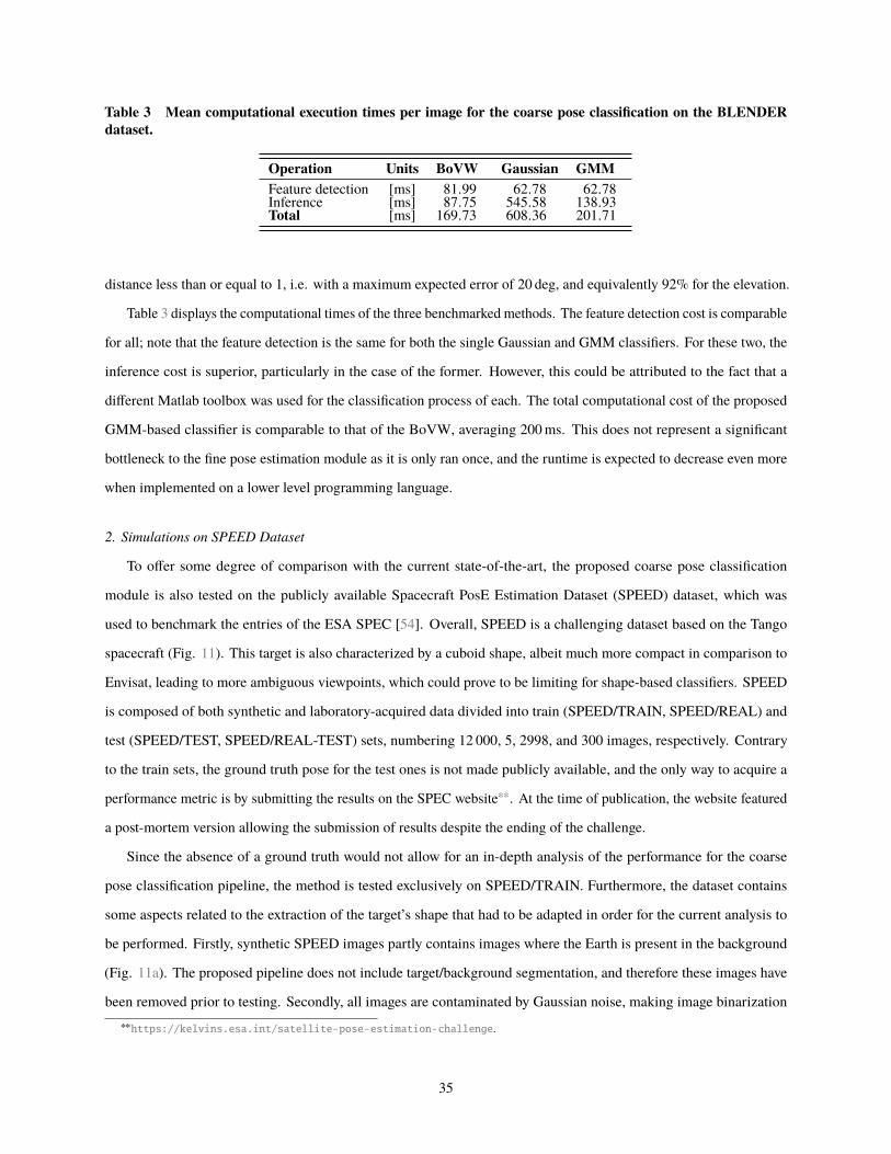
Table 3 Mean computational execution times per image for the coarse pose classification on the BLENDER

dataset.

Operation Units BoVW Gaussian GMM

Feature detection [ms] 81.99 62.78 62.78Inference [ms] 87.75 545.58 138.93Total [ms] 169.73 608.36 201.71

distance less than or equal to 1, i.e. with a maximum expected error of 20 deg, and equivalently 92% for the elevation.

Table 3 displays the computational times of the three benchmarked methods. The feature detection cost is comparable

for all; note that the feature detection is the same for both the single Gaussian and GMM classifiers. For these two, the

inference cost is superior, particularly in the case of the former. However, this could be attributed to the fact that a

different Matlab toolbox was used for the classification process of each. The total computational cost of the proposed

GMM-based classifier is comparable to that of the BoVW, averaging 200 ms. This does not represent a significant

bottleneck to the fine pose estimation module as it is only ran once, and the runtime is expected to decrease even more

when implemented on a lower level programming language.

2. Simulations on SPEED Dataset

To offer some degree of comparison with the current state-of-the-art, the proposed coarse pose classification

module is also tested on the publicly available Spacecraft PosE Estimation Dataset (SPEED) dataset, which was

used to benchmark the entries of the ESA SPEC [54]. Overall, SPEED is a challenging dataset based on the Tango

spacecraft (Fig. 11). This target is also characterized by a cuboid shape, albeit much more compact in comparison to

Envisat, leading to more ambiguous viewpoints, which could prove to be limiting for shape-based classifiers. SPEED

is composed of both synthetic and laboratory-acquired data divided into train (SPEED/TRAIN, SPEED/REAL) and

test (SPEED/TEST, SPEED/REAL-TEST) sets, numbering 12 000, 5, 2998, and 300 images, respectively. Contrary

to the train sets, the ground truth pose for the test ones is not made publicly available, and the only way to acquire a

performance metric is by submitting the results on the SPEC website∗∗. At the time of publication, the website featured

a post-mortem version allowing the submission of results despite the ending of the challenge.

Since the absence of a ground truth would not allow for an in-depth analysis of the performance for the coarse

pose classification pipeline, the method is tested exclusively on SPEED/TRAIN. Furthermore, the dataset contains

some aspects related to the extraction of the target’s shape that had to be adapted in order for the current analysis to

be performed. Firstly, synthetic SPEED images partly contains images where the Earth is present in the background

(Fig. 11a). The proposed pipeline does not include target/background segmentation, and therefore these images have

been removed prior to testing. Secondly, all images are contaminated by Gaussian noise, making image binarization

∗∗https://kelvins.esa.int/satellite-pose-estimation-challenge.

35

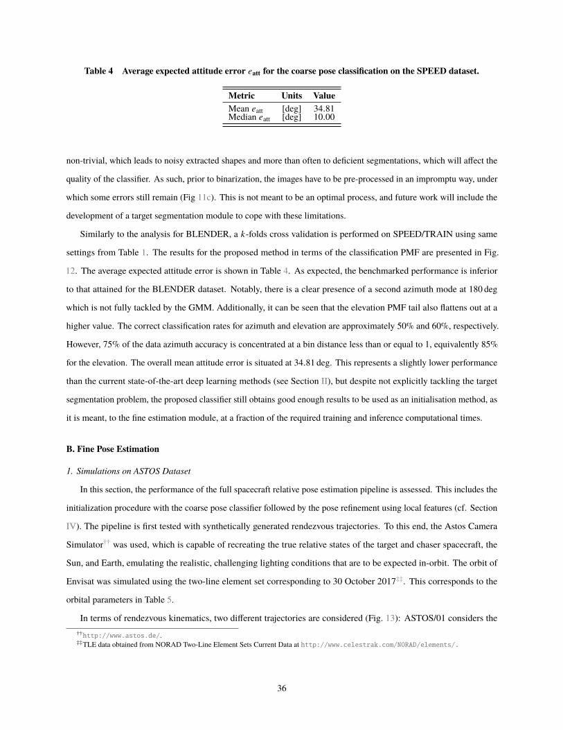
Table 4 Average expected attitude error 4att for the coarse pose classification on the SPEED dataset.

Metric Units Value

Mean 4att [deg] 34.81Median 4att [deg] 10.00

non-trivial, which leads to noisy extracted shapes and more than often to deficient segmentations, which will affect the

quality of the classifier. As such, prior to binarization, the images have to be pre-processed in an impromptu way, under

which some errors still remain (Fig 11c). This is not meant to be an optimal process, and future work will include the

development of a target segmentation module to cope with these limitations.

Similarly to the analysis for BLENDER, a :-folds cross validation is performed on SPEED/TRAIN using same

settings from Table 1. The results for the proposed method in terms of the classification PMF are presented in Fig.

12. The average expected attitude error is shown in Table 4. As expected, the benchmarked performance is inferior

to that attained for the BLENDER dataset. Notably, there is a clear presence of a second azimuth mode at 180 deg

which is not fully tackled by the GMM. Additionally, it can be seen that the elevation PMF tail also flattens out at a

higher value. The correct classification rates for azimuth and elevation are approximately 50% and 60%, respectively.

However, 75% of the data azimuth accuracy is concentrated at a bin distance less than or equal to 1, equivalently 85%

for the elevation. The overall mean attitude error is situated at 34.81 deg. This represents a slightly lower performance

than the current state-of-the-art deep learning methods (see Section II), but despite not explicitly tackling the target

segmentation problem, the proposed classifier still obtains good enough results to be used as an initialisation method, as

it is meant, to the fine estimation module, at a fraction of the required training and inference computational times.

B. Fine Pose Estimation

1. Simulations on ASTOS Dataset

In this section, the performance of the full spacecraft relative pose estimation pipeline is assessed. This includes the

initialization procedure with the coarse pose classifier followed by the pose refinement using local features (cf. Section

IV). The pipeline is first tested with synthetically generated rendezvous trajectories. To this end, the Astos Camera

Simulator†† was used, which is capable of recreating the true relative states of the target and chaser spacecraft, the

Sun, and Earth, emulating the realistic, challenging lighting conditions that are to be expected in-orbit. The orbit of

Envisat was simulated using the two-line element set corresponding to 30 October 2017‡‡. This corresponds to the

orbital parameters in Table 5.

In terms of rendezvous kinematics, two different trajectories are considered (Fig. 13): ASTOS/01 considers the

††http://www.astos.de/.‡‡TLE data obtained from NORAD Two-Line Element Sets Current Data at http://www.celestrak.com/NORAD/elements/.

36

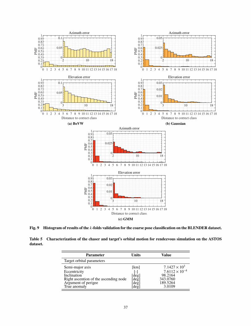
Azimuth error

0 1 2 3 4 5 6 7 8 9 10 11 12 13 14 15 16 17 180

0.1

0.2

0.3

0.4

0.5

0.6

0.7

0.8

0.9

1P

MF

2 10 180

0.05

0.1

Elevation error

0 1 2 3 4 5 6 7 8 9 10 11 12 13 14 15 16 17 18

Distance to correct class

0

0.1

0.2

0.3

0.4

0.5

0.6

0.7

0.8

0.9

1

PM

F

3 10 180

0.05

0.1

(a) BoVW

Azimuth error

0 1 2 3 4 5 6 7 8 9 10 11 12 13 14 15 16 17 180

0.1

0.2

0.3

0.4

0.5

0.6

0.7

0.8

0.9

1

PM

F

2 10 180

0.025

0.05

Elevation error

0 1 2 3 4 5 6 7 8 9 10 11 12 13 14 15 16 17 18

Distance to correct class

0

0.1

0.2

0.3

0.4

0.5

0.6

0.7

0.8

0.9

1

PM

F

3 10 180

0.01

0.02

0.03

(b) Gaussian

Azimuth error

0 1 2 3 4 5 6 7 8 9 10 11 12 13 14 15 16 17 180

0.1

0.2

0.3

0.4

0.5

0.6

0.7

0.8

0.9

1

PM

F

2 10 180

0.025

0.05

Elevation error

0 1 2 3 4 5 6 7 8 9 10 11 12 13 14 15 16 17 18

Distance to correct class

0

0.1

0.2

0.3

0.4

0.5

0.6

0.7

0.8

0.9

1

PM

F

3 10 180

0.01

0.02

0.03

(c) GMM

Fig. 9 Histogram of results of the :-folds validation for the coarse pose classification on the BLENDER dataset.

Table 5 Characterization of the chaser and target’s orbital motion for rendezvous simulation on the ASTOS

dataset.

Parameter Units Value

Target orbital parameters

Semi-major axis [km] 7.1427 × 103

Eccentricity [-] 7.6112 × 10−4

Inclination [deg] 98.2164Right ascention of the ascending node [deg] 343.0760Argument of perigee [deg] 189.5264True anomaly [deg] 3.0109

37

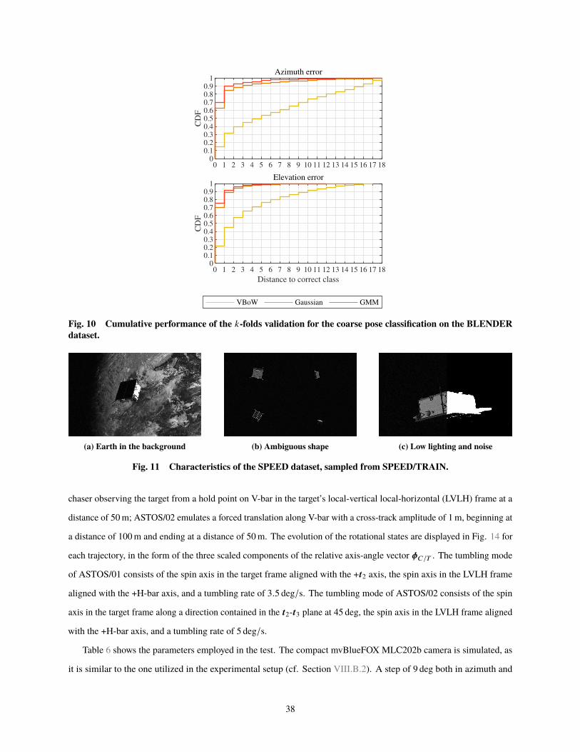
0 1 2 3 4 5 6 7 8 9 10 11 12 13 14 15 16 17 180

0.1

0.2

0.3

0.4

0.5

0.6

0.7

0.8

0.9

1

CD

F

Azimuth error

0 1 2 3 4 5 6 7 8 9 10 11 12 13 14 15 16 17 18

Distance to correct class

0

0.1

0.2

0.3

0.4

0.5

0.6

0.7

0.8

0.9

1

CD

F

Elevation error

VBoW Gaussian GMM

Fig. 10 Cumulative performance of the :-folds validation for the coarse pose classification on the BLENDER

dataset.

(a) Earth in the background (b) Ambiguous shape (c) Low lighting and noise

Fig. 11 Characteristics of the SPEED dataset, sampled from SPEED/TRAIN.

chaser observing the target from a hold point on V-bar in the target’s local-vertical local-horizontal (LVLH) frame at a

distance of 50 m; ASTOS/02 emulates a forced translation along V-bar with a cross-track amplitude of 1 m, beginning at

a distance of 100 m and ending at a distance of 50 m. The evolution of the rotational states are displayed in Fig. 14 for

each trajectory, in the form of the three scaled components of the relative axis-angle vector 5�/) . The tumbling mode

of ASTOS/01 consists of the spin axis in the target frame aligned with the +t2 axis, the spin axis in the LVLH frame

aligned with the +H-bar axis, and a tumbling rate of 3.5 deg/s. The tumbling mode of ASTOS/02 consists of the spin

axis in the target frame along a direction contained in the t2-t3 plane at 45 deg, the spin axis in the LVLH frame aligned

with the +H-bar axis, and a tumbling rate of 5 deg/s.

Table 6 shows the parameters employed in the test. The compact mvBlueFOX MLC202b camera is simulated, as

it is similar to the one utilized in the experimental setup (cf. Section VIII.B.2). A step of 9 deg both in azimuth and

38

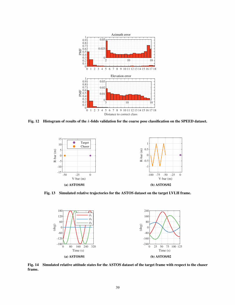
Azimuth error

0 1 2 3 4 5 6 7 8 9 10 11 12 13 14 15 16 17 180

0.1

0.2

0.3

0.4

0.5

0.6

0.7

0.8

0.9

1

PM

F

2 10 180

0.025

0.05

Elevation error

0 1 2 3 4 5 6 7 8 9 10 11 12 13 14 15 16 17 18

Distance to correct class

0

0.1

0.2

0.3

0.4

0.5

0.6

0.7

0.8

0.9

1P

MF

3 10 180

0.01

0.02

0.03

Fig. 12 Histogram of results of the :-folds validation for the coarse pose classification on the SPEED dataset.

-50 -25 0

V-bar (m)

-15

-10

-5

0

5

10

15

R-b

ar (

m)

Target

Chaser

(a) ASTOS/01

-100 -75 -50 -25 0

V-bar (m)

-1

-0.5

0

0.5

1R

-bar

(m)

(b) ASTOS/02

Fig. 13 Simulated relative trajectories for the ASTOS dataset on the target LVLH frame.

0 80 160 240 320

Time (s)

-180

-120

-60

0

60

120

180

(deg

)

(a) ASTOS/01

0 25 50 75 100 125

Time (s)

-240

-160

-80

0

80

160

240

(deg

)

(b) ASTOS/02

Fig. 14 Simulated relative attitude states for the ASTOS dataset of the target frame with respect to the chaser

frame.

39

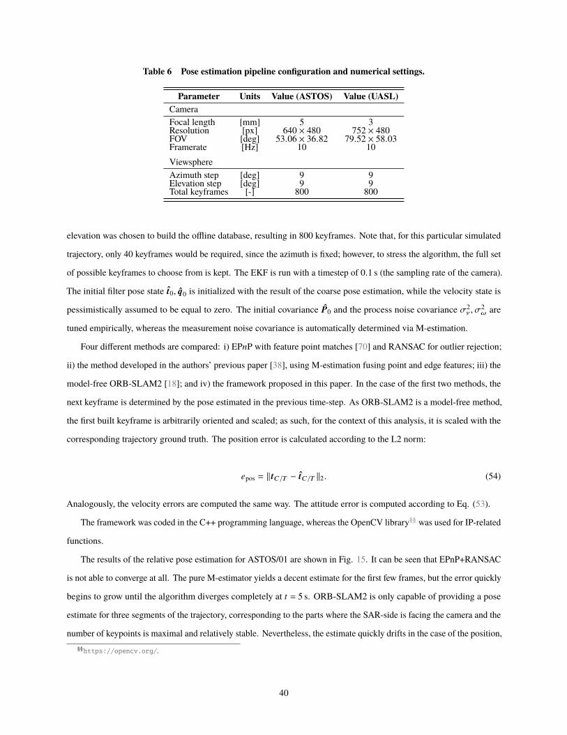
Table 6 Pose estimation pipeline configuration and numerical settings.

Parameter Units Value (ASTOS) Value (UASL)

Camera

Focal length [mm] 5 3Resolution [px] 640 × 480 752 × 480FOV [deg] 53.06 × 36.82 79.52 × 58.03Framerate [Hz] 10 10

Viewsphere

Azimuth step [deg] 9 9Elevation step [deg] 9 9Total keyframes [-] 800 800

elevation was chosen to build the offline database, resulting in 800 keyframes. Note that, for this particular simulated

trajectory, only 40 keyframes would be required, since the azimuth is fixed; however, to stress the algorithm, the full set

of possible keyframes to choose from is kept. The EKF is run with a timestep of 0.1 s (the sampling rate of the camera).

The initial filter pose state t0, q0 is initialized with the result of the coarse pose estimation, while the velocity state is

pessimistically assumed to be equal to zero. The initial covariance V0 and the process noise covariance f2a , f

2l are

tuned empirically, whereas the measurement noise covariance is automatically determined via M-estimation.

Four different methods are compared: i) EP=P with feature point matches [70] and RANSAC for outlier rejection;

ii) the method developed in the authors’ previous paper [38], using M-estimation fusing point and edge features; iii) the

model-free ORB-SLAM2 [18]; and iv) the framework proposed in this paper. In the case of the first two methods, the

next keyframe is determined by the pose estimated in the previous time-step. As ORB-SLAM2 is a model-free method,

the first built keyframe is arbitrarily oriented and scaled; as such, for the context of this analysis, it is scaled with the

corresponding trajectory ground truth. The position error is calculated according to the L2 norm:

4pos = ‖ t�/) − t�/) ‖2. (54)

Analogously, the velocity errors are computed the same way. The attitude error is computed according to Eq. (53).

The framework was coded in the C++ programming language, whereas the OpenCV library§§ was used for IP-related

functions.

The results of the relative pose estimation for ASTOS/01 are shown in Fig. 15. It can be seen that EPnP+RANSAC

is not able to converge at all. The pure M-estimator yields a decent estimate for the first few frames, but the error quickly

begins to grow until the algorithm diverges completely at C = 5 s. ORB-SLAM2 is only capable of providing a pose

estimate for three segments of the trajectory, corresponding to the parts where the SAR-side is facing the camera and the

number of keypoints is maximal and relatively stable. Nevertheless, the estimate quickly drifts in the case of the position,

§§https://opencv.org/.

40

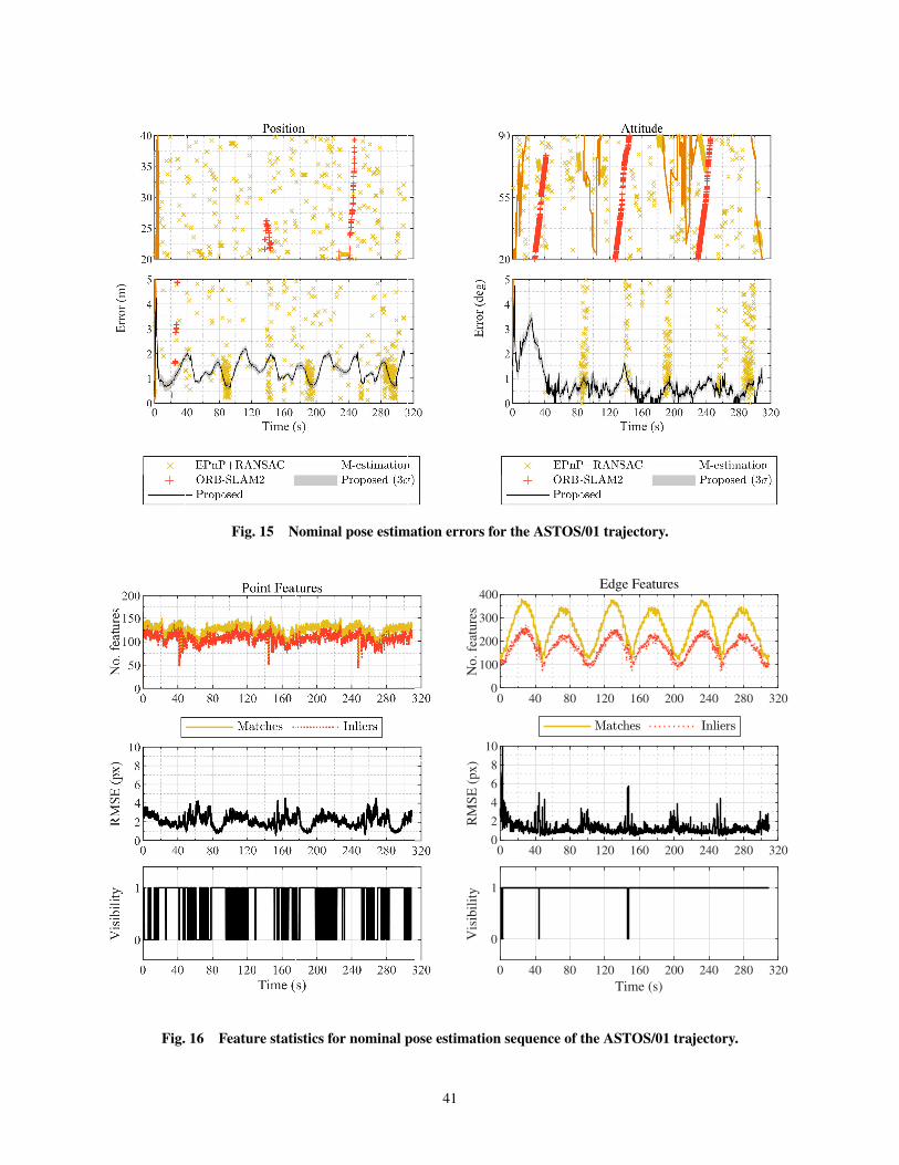
Fig. 15 Nominal pose estimation errors for the ASTOS/01 trajectory.

0 40 80 120 160 200 240 280 3200

100

200

300

400Edge Features

No. fe

ature

s

0 40 80 120 160 200 240 280 3200

2

4

6

8

10

RM

SE

(px)

0 40 80 120 160 200 240 280 320

Time (s)

0

1

Vis

ibil

ity

Fig. 16 Feature statistics for nominal pose estimation sequence of the ASTOS/01 trajectory.

41

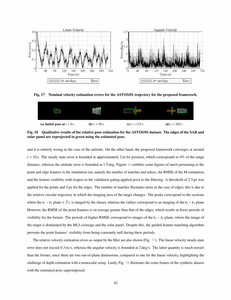
Fig. 17 Nominal velocity estimation errors for the ASTOS/01 trajectory for the proposed framework.

(a) Initial pose at C = 0 s (b) C = 50 s (c) C = 115 s (d) C = 285 s

Fig. 18 Qualitative results of the relative pose estimation for the ASTOS/01 dataset. The edges of the SAR and

solar panel are reprojected in green using the estimated pose.

and it is entirely wrong in the case of the attitude. On the other hand, the proposed framework converges at around

C = 10 s. The steady state error is bounded at approximately 2 m for position, which corresponds to 4% of the range

distance, whereas the attitude error is bounded at 1.5 deg. Figure 16 exhibits some figures of merit pertaining to the

point and edge features in the simulation run, namely the number of matches and inliers, the RMSE of the M-estimation,

and the feature visibility with respect to the validation gating applied prior to the filtering. A threshold of 2.5 px was

applied for the points and 5 px for the edges. The number of matches fluctuates more in the case of edges; this is due to

the relative circular trajectory in which the imaging area of the target changes. The peaks correspond to the sections

where the t1 − t2 plane ∈ FT is imaged by the chaser, whereas the valleys correspond to an imaging of the t2 − t3 plane.

However, the RMSE of the point features is on average greater than that of the edges, which results in fewer periods of

visibility for the former. The periods of higher RMSE correspond to images of the t1 − t2 plane, where the image of

the target is dominated by the MLI coverage and the solar panel. Despite this, the guided feature matching algorithm

prevents the point features’ visibility from being constantly null during these periods.

The relative velocity estimation errors as output by the filter are also shown (Fig. 17). The linear velocity steady-state

error does not exceed 0.3 m/s, whereas the angular velocity is bounded at 2 deg/s. The latter quantity is much noisier

than the former, since there are two out-of-plane dimensions, compared to one for the linear velocity, highlighting the

challenge of depth estimation with a monocular setup. Lastly, Fig. 18 illustrates the some frames of the synthetic dataset

with the estimated pose superimposed.

42

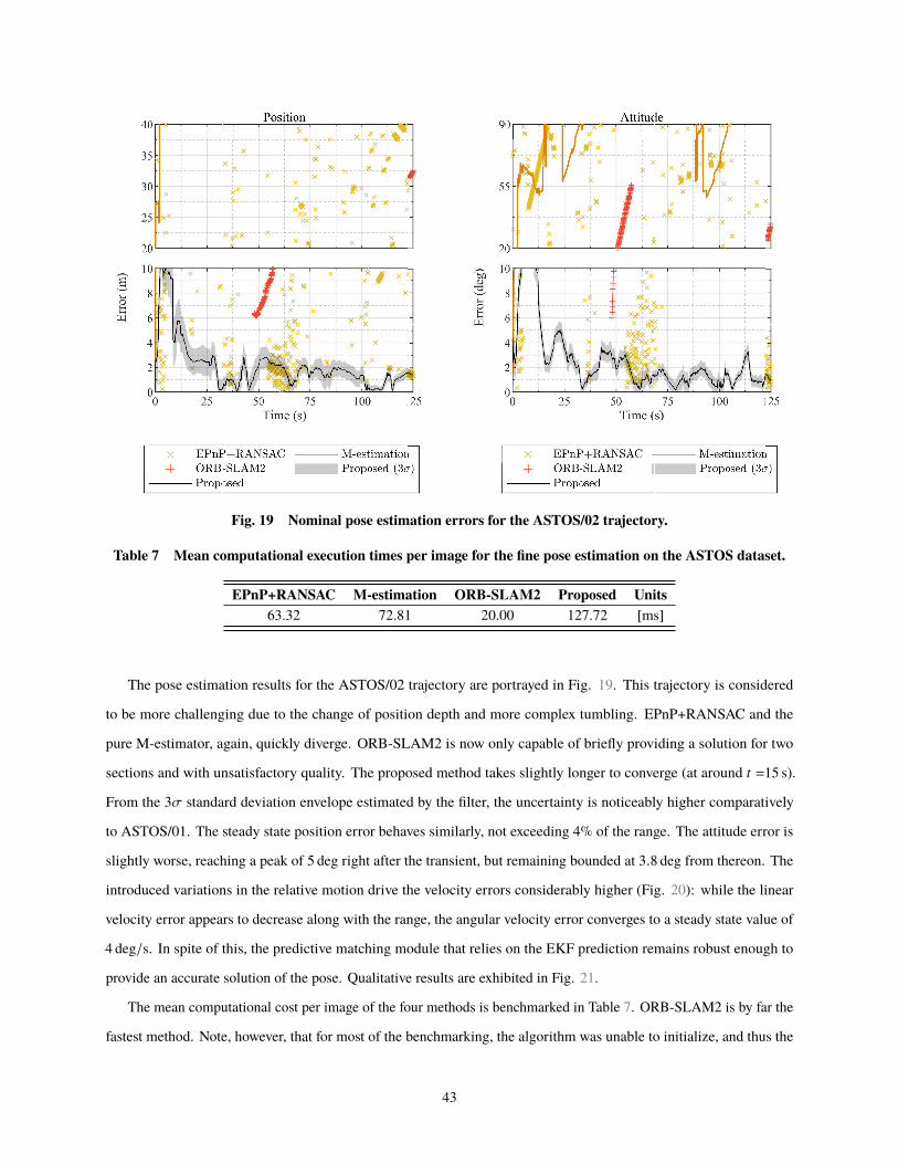
Fig. 19 Nominal pose estimation errors for the ASTOS/02 trajectory.

Table 7 Mean computational execution times per image for the fine pose estimation on the ASTOS dataset.

EPnP+RANSAC M-estimation ORB-SLAM2 Proposed Units

63.32 72.81 20.00 127.72 [ms]

The pose estimation results for the ASTOS/02 trajectory are portrayed in Fig. 19. This trajectory is considered

to be more challenging due to the change of position depth and more complex tumbling. EPnP+RANSAC and the

pure M-estimator, again, quickly diverge. ORB-SLAM2 is now only capable of briefly providing a solution for two

sections and with unsatisfactory quality. The proposed method takes slightly longer to converge (at around C =15 s).

From the 3f standard deviation envelope estimated by the filter, the uncertainty is noticeably higher comparatively

to ASTOS/01. The steady state position error behaves similarly, not exceeding 4% of the range. The attitude error is

slightly worse, reaching a peak of 5 deg right after the transient, but remaining bounded at 3.8 deg from thereon. The

introduced variations in the relative motion drive the velocity errors considerably higher (Fig. 20): while the linear

velocity error appears to decrease along with the range, the angular velocity error converges to a steady state value of

4 deg/s. In spite of this, the predictive matching module that relies on the EKF prediction remains robust enough to

provide an accurate solution of the pose. Qualitative results are exhibited in Fig. 21.

The mean computational cost per image of the four methods is benchmarked in Table 7. ORB-SLAM2 is by far the

fastest method. Note, however, that for most of the benchmarking, the algorithm was unable to initialize, and thus the

43

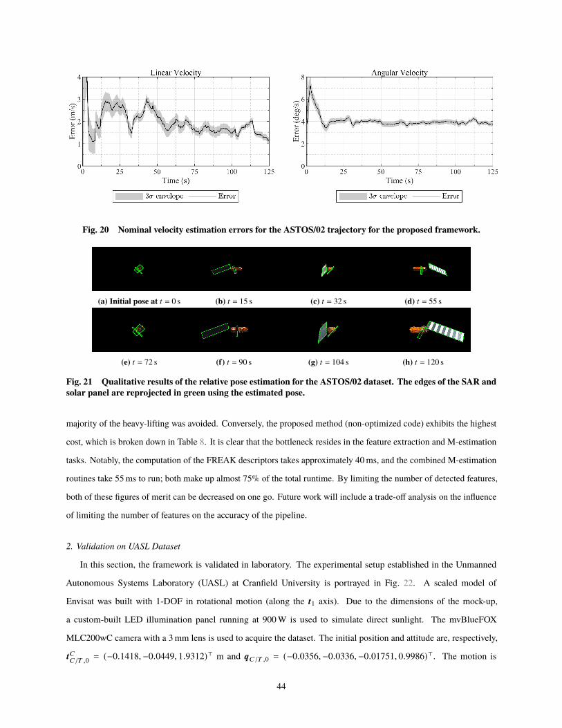
Fig. 20 Nominal velocity estimation errors for the ASTOS/02 trajectory for the proposed framework.

(a) Initial pose at C = 0 s (b) C = 15 s (c) C = 32 s (d) C = 55 s

(e) C = 72 s (f) C = 90 s (g) C = 104 s (h) C = 120 s

Fig. 21 Qualitative results of the relative pose estimation for the ASTOS/02 dataset. The edges of the SAR and

solar panel are reprojected in green using the estimated pose.

majority of the heavy-lifting was avoided. Conversely, the proposed method (non-optimized code) exhibits the highest

cost, which is broken down in Table 8. It is clear that the bottleneck resides in the feature extraction and M-estimation

tasks. Notably, the computation of the FREAK descriptors takes approximately 40 ms, and the combined M-estimation

routines take 55 ms to run; both make up almost 75% of the total runtime. By limiting the number of detected features,

both of these figures of merit can be decreased on one go. Future work will include a trade-off analysis on the influence

of limiting the number of features on the accuracy of the pipeline.

2. Validation on UASL Dataset

In this section, the framework is validated in laboratory. The experimental setup established in the Unmanned

Autonomous Systems Laboratory (UASL) at Cranfield University is portrayed in Fig. 22. A scaled model of

Envisat was built with 1-DOF in rotational motion (along the t1 axis). Due to the dimensions of the mock-up,

a custom-built LED illumination panel running at 900 W is used to simulate direct sunlight. The mvBlueFOX

MLC200wC camera with a 3 mm lens is used to acquire the dataset. The initial position and attitude are, respectively,

t��/) ,0

= (−0.1418,−0.0449, 1.9312)⊤ m and q�/) ,0 = (−0.0356,−0.0336,−0.01751, 0.9986)⊤. The motion is

44

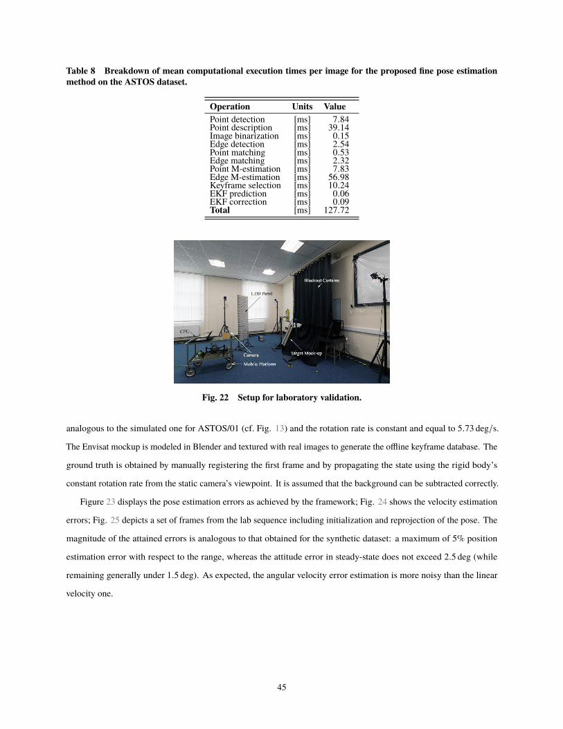
Table 8 Breakdown of mean computational execution times per image for the proposed fine pose estimation

method on the ASTOS dataset.

Operation Units Value

Point detection [ms] 7.84Point description [ms] 39.14Image binarization [ms] 0.15Edge detection [ms] 2.54Point matching [ms] 0.53Edge matching [ms] 2.32Point M-estimation [ms] 7.83Edge M-estimation [ms] 56.98Keyframe selection [ms] 10.24EKF prediction [ms] 0.06EKF correction [ms] 0.09Total [ms] 127.72

Fig. 22 Setup for laboratory validation.

analogous to the simulated one for ASTOS/01 (cf. Fig. 13) and the rotation rate is constant and equal to 5.73 deg/s.

The Envisat mockup is modeled in Blender and textured with real images to generate the offline keyframe database. The

ground truth is obtained by manually registering the first frame and by propagating the state using the rigid body’s

constant rotation rate from the static camera’s viewpoint. It is assumed that the background can be subtracted correctly.

Figure 23 displays the pose estimation errors as achieved by the framework; Fig. 24 shows the velocity estimation

errors; Fig. 25 depicts a set of frames from the lab sequence including initialization and reprojection of the pose. The

magnitude of the attained errors is analogous to that obtained for the synthetic dataset: a maximum of 5% position

estimation error with respect to the range, whereas the attitude error in steady-state does not exceed 2.5 deg (while

remaining generally under 1.5 deg). As expected, the angular velocity error estimation is more noisy than the linear

velocity one.

45

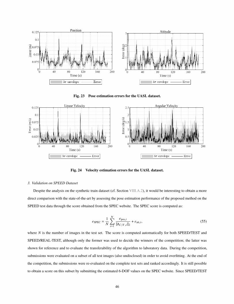
Fig. 23 Pose estimation errors for the UASL dataset.

Fig. 24 Velocity estimation errors for the UASL dataset.

3. Validation on SPEED Dataset

Despite the analysis on the synthetic train dataset (cf. Section VIII.A.2), it would be interesting to obtain a more

direct comparison with the state-of-the-art by assessing the pose estimation performance of the proposed method on the

SPEED test data through the score obtained from the SPEC website. The SPEC score is computed as:

4SPEC =1

#

#∑8=1

4pos,8

‖ t�/) ,8 ‖2+ 4att,8 , (55)

where # is the number of images in the test set. The score is computed automatically for both SPEED/TEST and

SPEED/REAL-TEST, although only the former was used to decide the winners of the competition; the latter was

shown for reference and to evaluate the transferability of the algorithm to laboratory data. During the competition,

submissions were evaluated on a subset of all test images (also undisclosed) in order to avoid overfitting. At the end of

the competition, the submissions were re-evaluated on the complete test sets and ranked accordingly. It is still possible

to obtain a score on this subset by submitting the estimated 6-DOF values on the SPEC website. Since SPEED/TEST

46

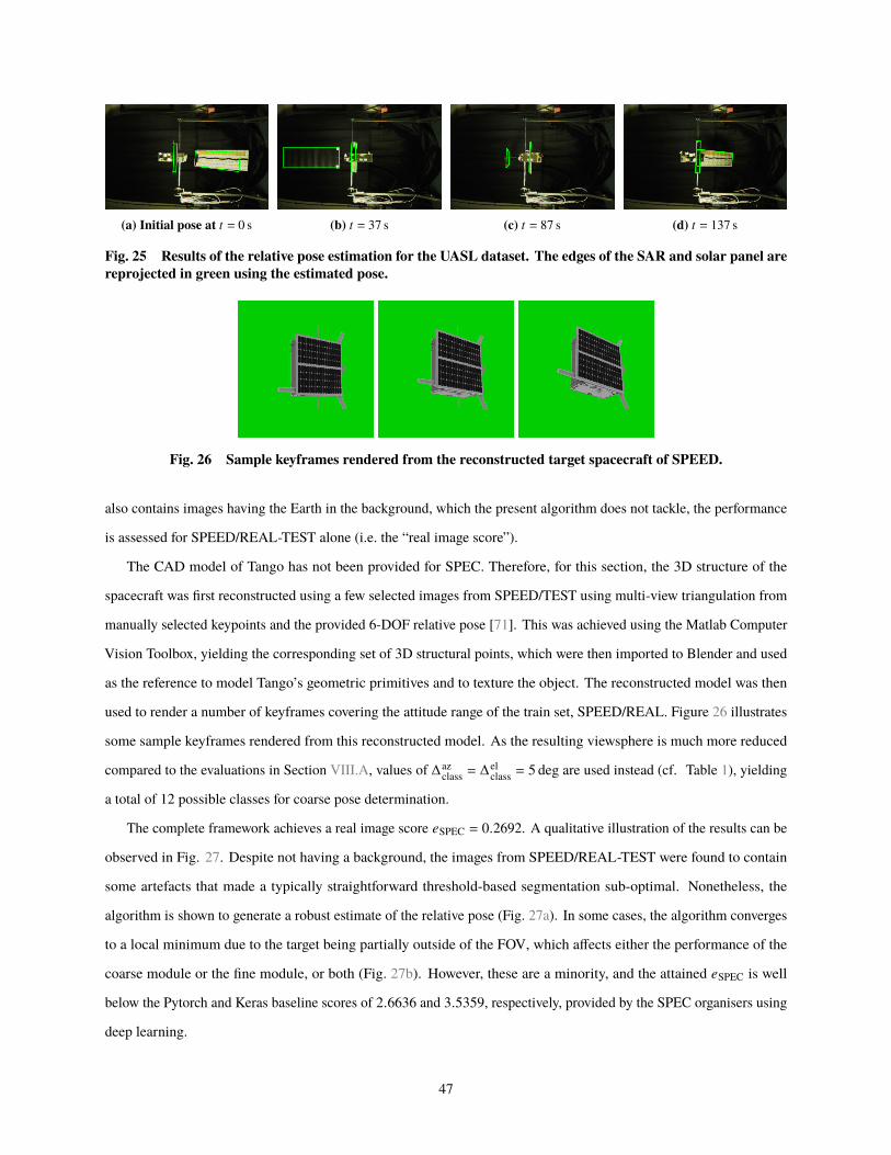
(a) Initial pose at C = 0 s (b) C = 37 s (c) C = 87 s (d) C = 137 s

Fig. 25 Results of the relative pose estimation for the UASL dataset. The edges of the SAR and solar panel are

reprojected in green using the estimated pose.

Fig. 26 Sample keyframes rendered from the reconstructed target spacecraft of SPEED.

also contains images having the Earth in the background, which the present algorithm does not tackle, the performance

is assessed for SPEED/REAL-TEST alone (i.e. the “real image score”).

The CAD model of Tango has not been provided for SPEC. Therefore, for this section, the 3D structure of the

spacecraft was first reconstructed using a few selected images from SPEED/TEST using multi-view triangulation from

manually selected keypoints and the provided 6-DOF relative pose [71]. This was achieved using the Matlab Computer

Vision Toolbox, yielding the corresponding set of 3D structural points, which were then imported to Blender and used

as the reference to model Tango’s geometric primitives and to texture the object. The reconstructed model was then

used to render a number of keyframes covering the attitude range of the train set, SPEED/REAL. Figure 26 illustrates

some sample keyframes rendered from this reconstructed model. As the resulting viewsphere is much more reduced

compared to the evaluations in Section VIII.A, values of Δazclass

= Δelclass

= 5 deg are used instead (cf. Table 1), yielding

a total of 12 possible classes for coarse pose determination.

The complete framework achieves a real image score 4SPEC = 0.2692. A qualitative illustration of the results can be

observed in Fig. 27. Despite not having a background, the images from SPEED/REAL-TEST were found to contain

some artefacts that made a typically straightforward threshold-based segmentation sub-optimal. Nonetheless, the

algorithm is shown to generate a robust estimate of the relative pose (Fig. 27a). In some cases, the algorithm converges

to a local minimum due to the target being partially outside of the FOV, which affects either the performance of the

coarse module or the fine module, or both (Fig. 27b). However, these are a minority, and the attained 4SPEC is well

below the Pytorch and Keras baseline scores of 2.6636 and 3.5359, respectively, provided by the SPEC organisers using

deep learning.

47

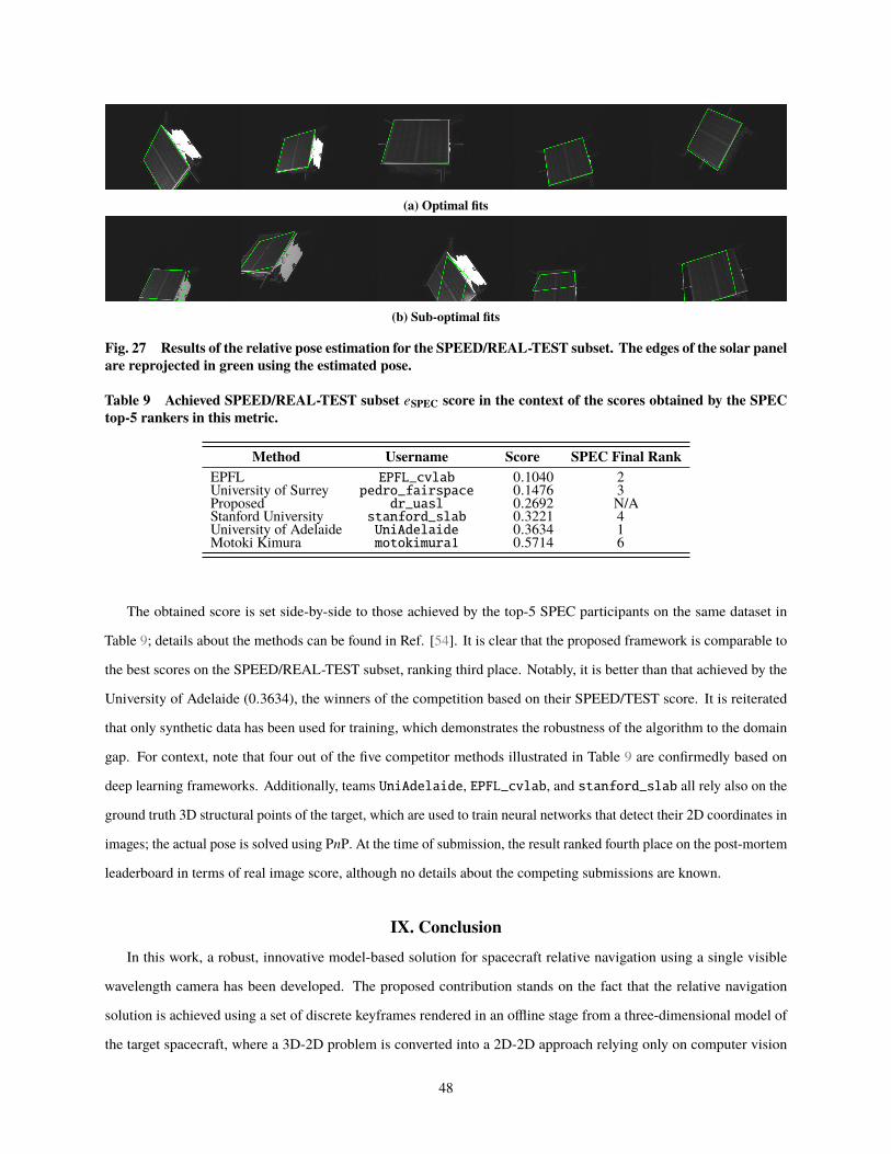
(a) Optimal fits

(b) Sub-optimal fits

Fig. 27 Results of the relative pose estimation for the SPEED/REAL-TEST subset. The edges of the solar panel

are reprojected in green using the estimated pose.

Table 9 Achieved SPEED/REAL-TEST subset 4SPEC score in the context of the scores obtained by the SPEC

top-5 rankers in this metric.

Method Username Score SPEC Final Rank

EPFL EPFL_cvlab 0.1040 2University of Surrey pedro_fairspace 0.1476 3Proposed dr_uasl 0.2692 N/AStanford University stanford_slab 0.3221 4University of Adelaide UniAdelaide 0.3634 1Motoki Kimura motokimura1 0.5714 6

The obtained score is set side-by-side to those achieved by the top-5 SPEC participants on the same dataset in

Table 9; details about the methods can be found in Ref. [54]. It is clear that the proposed framework is comparable to

the best scores on the SPEED/REAL-TEST subset, ranking third place. Notably, it is better than that achieved by the

University of Adelaide (0.3634), the winners of the competition based on their SPEED/TEST score. It is reiterated

that only synthetic data has been used for training, which demonstrates the robustness of the algorithm to the domain

gap. For context, note that four out of the five competitor methods illustrated in Table 9 are confirmedly based on

deep learning frameworks. Additionally, teams UniAdelaide, EPFL_cvlab, and stanford_slab all rely also on the

ground truth 3D structural points of the target, which are used to train neural networks that detect their 2D coordinates in

images; the actual pose is solved using P=P. At the time of submission, the result ranked fourth place on the post-mortem

leaderboard in terms of real image score, although no details about the competing submissions are known.

IX. Conclusion

In this work, a robust, innovative model-based solution for spacecraft relative navigation using a single visible

wavelength camera has been developed. The proposed contribution stands on the fact that the relative navigation

solution is achieved using a set of discrete keyframes rendered in an offline stage from a three-dimensional model of

the target spacecraft, where a 3D-2D problem is converted into a 2D-2D approach relying only on computer vision

48

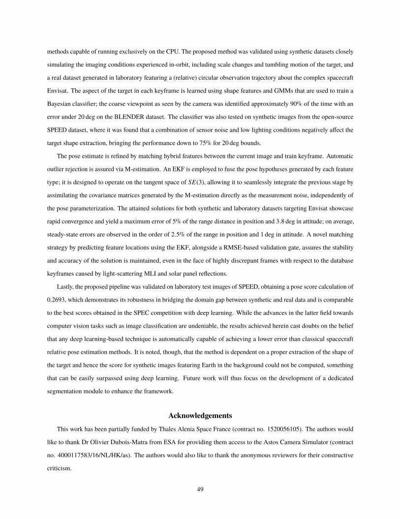
methods capable of running exclusively on the CPU. The proposed method was validated using synthetic datasets closely

simulating the imaging conditions experienced in-orbit, including scale changes and tumbling motion of the target, and

a real dataset generated in laboratory featuring a (relative) circular observation trajectory about the complex spacecraft

Envisat. The aspect of the target in each keyframe is learned using shape features and GMMs that are used to train a

Bayesian classifier; the coarse viewpoint as seen by the camera was identified approximately 90% of the time with an

error under 20 deg on the BLENDER dataset. The classifier was also tested on synthetic images from the open-source

SPEED dataset, where it was found that a combination of sensor noise and low lighting conditions negatively affect the

target shape extraction, bringing the performance down to 75% for 20 deg bounds.

The pose estimate is refined by matching hybrid features between the current image and train keyframe. Automatic

outlier rejection is assured via M-estimation. An EKF is employed to fuse the pose hypotheses generated by each feature

type; it is designed to operate on the tangent space of (�(3), allowing it to seamlessly integrate the previous stage by

assimilating the covariance matrices generated by the M-estimation directly as the measurement noise, independently of

the pose parameterization. The attained solutions for both synthetic and laboratory datasets targeting Envisat showcase

rapid convergence and yield a maximum error of 5% of the range distance in position and 3.8 deg in attitude; on average,

steady-state errors are observed in the order of 2.5% of the range in position and 1 deg in attitude. A novel matching

strategy by predicting feature locations using the EKF, alongside a RMSE-based validation gate, assures the stability

and accuracy of the solution is maintained, even in the face of highly discrepant frames with respect to the database

keyframes caused by light-scattering MLI and solar panel reflections.

Lastly, the proposed pipeline was validated on laboratory test images of SPEED, obtaining a pose score calculation of

0.2693, which demonstrates its robustness in bridging the domain gap between synthetic and real data and is comparable

to the best scores obtained in the SPEC competition with deep learning. While the advances in the latter field towards

computer vision tasks such as image classification are undeniable, the results achieved herein cast doubts on the belief

that any deep learning-based technique is automatically capable of achieving a lower error than classical spacecraft

relative pose estimation methods. It is noted, though, that the method is dependent on a proper extraction of the shape of

the target and hence the score for synthetic images featuring Earth in the background could not be computed, something

that can be easily surpassed using deep learning. Future work will thus focus on the development of a dedicated

segmentation module to enhance the framework.

Acknowledgements

This work has been partially funded by Thales Alenia Space France (contract no. 1520056105). The authors would

like to thank Dr Olivier Dubois-Matra from ESA for providing them access to the Astos Camera Simulator (contract

no. 4000117583/16/NL/HK/as). The authors would also like to thank the anonymous reviewers for their constructive

criticism.

49

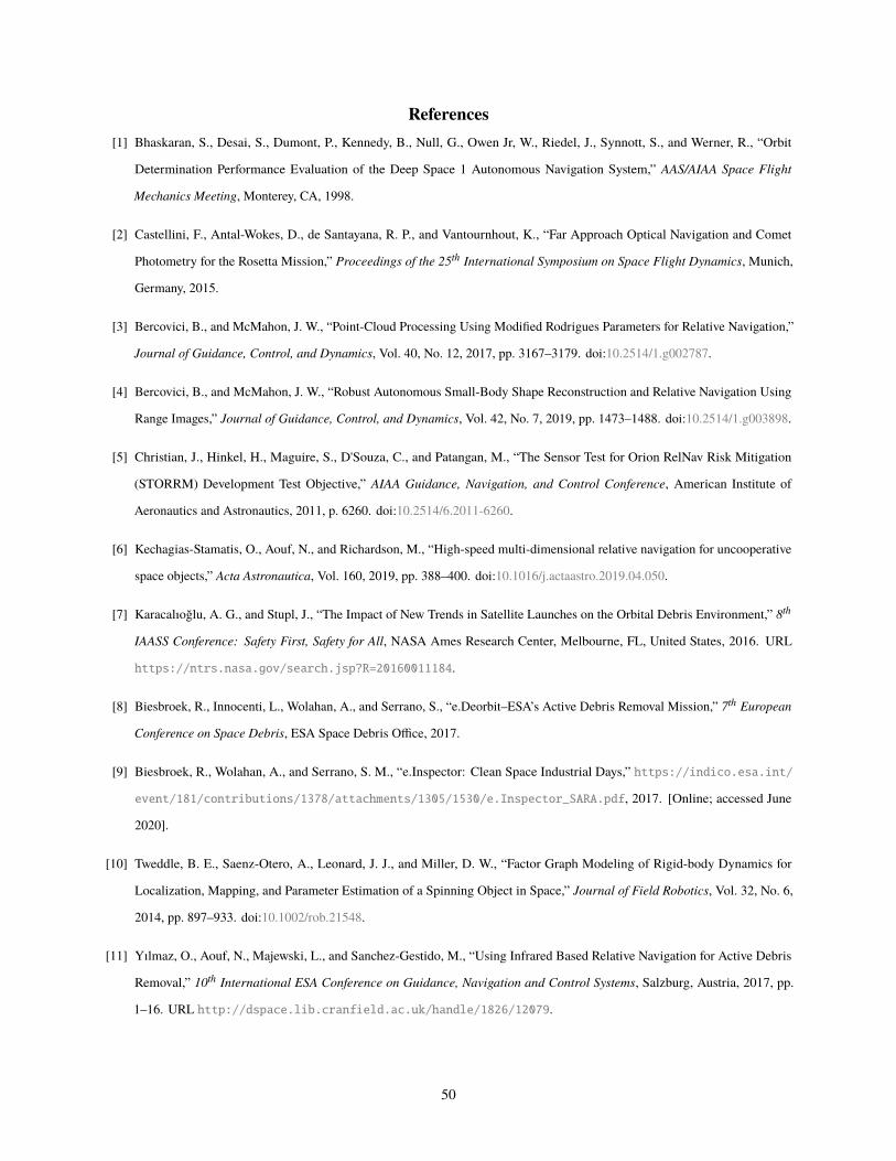
References

[1] Bhaskaran, S., Desai, S., Dumont, P., Kennedy, B., Null, G., Owen Jr, W., Riedel, J., Synnott, S., and Werner, R., “Orbit

Determination Performance Evaluation of the Deep Space 1 Autonomous Navigation System,” AAS/AIAA Space Flight

Mechanics Meeting, Monterey, CA, 1998.

[2] Castellini, F., Antal-Wokes, D., de Santayana, R. P., and Vantournhout, K., “Far Approach Optical Navigation and Comet

Photometry for the Rosetta Mission,” Proceedings of the 25th International Symposium on Space Flight Dynamics, Munich,

Germany, 2015.

[3] Bercovici, B., and McMahon, J. W., “Point-Cloud Processing Using Modified Rodrigues Parameters for Relative Navigation,”

Journal of Guidance, Control, and Dynamics, Vol. 40, No. 12, 2017, pp. 3167–3179. doi:10.2514/1.g002787.

[4] Bercovici, B., and McMahon, J. W., “Robust Autonomous Small-Body Shape Reconstruction and Relative Navigation Using

Range Images,” Journal of Guidance, Control, and Dynamics, Vol. 42, No. 7, 2019, pp. 1473–1488. doi:10.2514/1.g003898.

[5] Christian, J., Hinkel, H., Maguire, S., D'Souza, C., and Patangan, M., “The Sensor Test for Orion RelNav Risk Mitigation

(STORRM) Development Test Objective,” AIAA Guidance, Navigation, and Control Conference, American Institute of

Aeronautics and Astronautics, 2011, p. 6260. doi:10.2514/6.2011-6260.

[6] Kechagias-Stamatis, O., Aouf, N., and Richardson, M., “High-speed multi-dimensional relative navigation for uncooperative

space objects,” Acta Astronautica, Vol. 160, 2019, pp. 388–400. doi:10.1016/j.actaastro.2019.04.050.

[7] Karacalıoğlu, A. G., and Stupl, J., “The Impact of New Trends in Satellite Launches on the Orbital Debris Environment,” 8th

IAASS Conference: Safety First, Safety for All, NASA Ames Research Center, Melbourne, FL, United States, 2016. URL

https://ntrs.nasa.gov/search.jsp?R=20160011184.

[8] Biesbroek, R., Innocenti, L., Wolahan, A., and Serrano, S., “e.Deorbit–ESA’s Active Debris Removal Mission,” 7th European

Conference on Space Debris, ESA Space Debris Office, 2017.

[9] Biesbroek, R., Wolahan, A., and Serrano, S. M., “e.Inspector: Clean Space Industrial Days,” https://indico.esa.int/

event/181/contributions/1378/attachments/1305/1530/e.Inspector_SARA.pdf, 2017. [Online; accessed June

2020].

[10] Tweddle, B. E., Saenz-Otero, A., Leonard, J. J., and Miller, D. W., “Factor Graph Modeling of Rigid-body Dynamics for

Localization, Mapping, and Parameter Estimation of a Spinning Object in Space,” Journal of Field Robotics, Vol. 32, No. 6,

2014, pp. 897–933. doi:10.1002/rob.21548.

[11] Yılmaz, O., Aouf, N., Majewski, L., and Sanchez-Gestido, M., “Using Infrared Based Relative Navigation for Active Debris

Removal,” 10th International ESA Conference on Guidance, Navigation and Control Systems, Salzburg, Austria, 2017, pp.

1–16. URL http://dspace.lib.cranfield.ac.uk/handle/1826/12079.

50

[12] Lowe, D. G., “Distinctive Image Features from Scale-Invariant Keypoints,” International Journal of Computer Vision, Vol. 60,

No. 2, 2004, pp. 91–110. doi:10.1023/b:visi.0000029664.99615.94.

[13] Rublee, E., Rabaud, V., Konolige, K., and Bradski, G., “ORB: An Efficient Alternative to SIFT or SURF,” 2011 International

Conference on Computer Vision, IEEE, 2011, pp. 2564–2571. doi:10.1109/iccv.2011.6126544.

[14] Rondao, D., Aouf, N., Richardson, M. A., and Dubois-Matra, O., “Benchmarking of local feature detectors and descriptors for

multispectral relative navigation in space,” Acta Astronautica, Vol. 172, 2020, pp. 100–122. doi:10.1016/j.actaastro.2020.03.049.

[15] Lowe, D. G., “Three-Dimensional Object Recognition from Single Two-Dimensional Images,” Artificial Intelligence, Vol. 31,

No. 3, 1987, pp. 355–395. doi:10.1016/0004-3702(87)90070-1.

[16] Dhome, M., Richetin, M., Lapreste, J.-T., and Rives, G., “Determination of the Attitude of 3D Objects from a Single

Perspective View,” IEEE Transactions on Pattern Analysis and Machine Intelligence, Vol. 11, No. 12, 1989, pp. 1265–1278.

doi:10.1109/34.41365.

[17] “The vSLAM Algorithm for Robust Localization and Mapping,” Proceedings of the 2005 IEEE International Conference on

Robotics and Automation (ICRA), IEEE, 2005, pp. 24–29. doi:10.1109/robot.2005.1570091.

[18] Mur-Artal, R., Montiel, J. M. M., and Tardos, J. D., “ORB-SLAM: A Versatile and Accurate Monocular SLAM System,” IEEE

Transactions on Robotics, Vol. 31, No. 5, 2015, pp. 1147–1163. doi:10.1109/tro.2015.2463671.

[19] Engel, J., Schöps, T., and Cremers, D., “LSD-SLAM: Large-Scale Direct Monocular SLAM,” Computer Vision – ECCV 2014,

Springer International Publishing, 2014, pp. 834–849. doi:10.1007/978-3-319-10605-2_54.

[20] Augenstein, S., and Rock, S., “Simultaneous Estimation of Target Pose and 3-D Shape Using the FastSLAM Algorithm,” AIAA

Guidance, Navigation, and Control Conference, American Institute of Aeronautics and Astronautics, 2009. doi:10.2514/6.2009-

5782.

[21] Dor, M., and Tsiotras, P., “ORB-SLAM Applied to Spacecraft Non-Cooperative Rendezvous,” 2018 Space Flight Mechanics

Meeting, American Institute of Aeronautics and Astronautics, 2018. doi:10.2514/6.2018-1963.

[22] Lepetit, V., and Fua, P., “Monocular Model-Based 3D Tracking of Rigid Objects: A Survey,” Foundations and Trends in

Computer Graphics and Vision, Vol. 1, No. 1, 2005, pp. 1–89. doi:10.1561/0600000001.

[23] Comport, A., Marchand, E., Pressigout, M., and Chaumette, F., “Real-Time Markerless Tracking for Augmented Reality: the

Virtual Visual Servoing Framework,” IEEE Transactions on Visualization and Computer Graphics, Vol. 12, No. 4, 2006, pp.

615–628. doi:10.1109/tvcg.2006.78.

[24] Kelsey, J., Byrne, J., Cosgrove, M., Seereeram, S., and Mehra, R., “Vision-Based Relative Pose Estimation for Autonomous

Rendezvous And Docking,” 2006 IEEE Aerospace Conference, IEEE, 2006. doi:10.1109/aero.2006.1655916.

[25] Petit, A., Marchand, E., and Kanani, K., “A Robust Model-Based Tracker Combining Geometrical and Color Edge Information,”

2013 IEEE/RSJ International Conference on Intelligent Robots and Systems, IEEE, 2013. doi:10.1109/iros.2013.6696887.

51

[26] Zou, Y., Wang, X., Zhang, T., and Song, J., “Combining Point and Edge for Satellite Pose Tracking Under Illumination Varying,”

2016 12th World Congress on Intelligent Control and Automation (WCICA), IEEE, 2016. doi:10.1109/wcica.2016.7578814.

[27] Oumer, N. W., “Monocular 3D Pose Tracking of a Specular Object,” Proceedings of the 9th International Confer-

ence on Computer Vision Theory and Applications, SCITEPRESS - Science and and Technology Publications, 2014.

doi:10.5220/0004667304580465.

[28] Cai, J., Huang, P., Zhang, B., and Wang, D., “A TSR Visual Servoing System Based on a Novel Dynamic Template Matching

Method,” Sensors, Vol. 15, No. 12, 2015, pp. 32152–32167. doi:10.3390/s151229884.

[29] Gansmann, M., Mongrard, O., and Ankersen, F., “3D Model-Based Relative Pose Estimation for Rendezvous and Docking

Using Edge Features,” 10th International ESA Conference on Guidance, Navigation and Control Systems, 2017.

[30] Vacchetti, L., Lepetit, V., and Fua, P., “Fusing Online and Offline Information for Stable 3D Tracking in Real-Time,” Computer

Society Conference on Computer Vision and Pattern Recognition Proceedings, Vol. 2, IEEE, 2003, pp. II–241.

[31] Cropp, A., “Pose Estimation and Relative Orbit Determination of a Nearby Target Microsatellite using Passive Imagery,” Ph.D.

thesis, University of Surrey, United Kingdom, 2001. URL http://epubs.surrey.ac.uk/843875/.

[32] Lowe, D., “Fitting Parameterized Three-Dimensional Models to Images,” IEEE Transactions on Pattern Analysis and Machine

Intelligence, Vol. 13, No. 5, 1991, pp. 441–450. doi:10.1109/34.134043.

[33] Abdenrahim, M., Diaz, J., Rossi, C., and Salichs, M., “Experimental Simulation of Satellite Relative Navigation Using

Computer Vision,” Proceedings of 2nd International Conference on Recent Advances in Space Technologies (RAST), IEEE,

2005. doi:10.1109/rast.2005.1512596.

[34] Liu, C., and Hu, W., “Relative Pose Estimation for Cylinder-Shaped Spacecrafts using Single Image,” IEEE Transactions on

Aerospace and Electronic Systems, Vol. 50, No. 4, 2014, pp. 3036–3056. doi:10.1109/taes.2014.120757.

[35] Shi, J., Ulrich, S., and Ruel, S., “Spacecraft Pose Estimation Using a Monocular Camera,” 67th International Astronautical

Congress, Guadalajara, Mexico, 2016.

[36] Post, M., and Li, J., “Visual Monocular 3D Reconstruction and Component Identification for Small Spacecraft,” 2018.

doi:10.20944/preprints201801.0195.v1, Multidisciplinary Digital Publishing Institute (preprint).

[37] Kechagias-Stamatis, O., and Aouf, N., “Histogram of Distances for Local Surface Description,” 2016 IEEE International

Conference on Robotics and Automation (ICRA), IEEE, 2016. doi:10.1109/icra.2016.7487402.

[38] Rondao, D., and Aouf, N., “Multi-View Monocular Pose Estimation for Spacecraft Relative Navigation,” 2018 AIAA Guidance,

Navigation, and Control Conference, American Institute of Aeronautics and Astronautics, 2018. doi:10.2514/6.2018-2100.

[39] Dudani, S. A., Breeding, K. J., and McGhee, R. B., “Aircraft Identification by Moment Invariants,” IEEE Transactions on

Computers, Vol. C-26, No. 1, 1977, pp. 39–46. doi:10.1109/tc.1977.5009272.

52

[40] Reeves, A., Prokop, R., Andrews, S., and Kuhl, F., “Three-Dimensional Shape Analysis Using Moments and Fourier Descriptors,”

IEEE Transactions on Pattern Analysis and Machine Intelligence, Vol. 10, No. 6, 1988, pp. 937–943. doi:10.1109/34.9115.

[41] Breuers, M. G. J., “Image-based Aircraft Pose Estimation using Moment Invariants,” Automatic Target Recognition IX, edited

by F. A. Sadjadi, SPIE, 1999. doi:10.1117/12.359963.

[42] Ozuysal, M., Lepetit, V., and Fua, P., “Pose Estimation for Category Specific Multiview Object Localization,” 2009 IEEE

Conference on Computer Vision and Pattern Recognition, IEEE, 2009. doi:10.1109/cvpr.2009.5206633.

[43] Glasner, D., Galun, M., Alpert, S., Basri, R., and Shakhnarovich, G., “Viewpoint-Aware Object Detection and Pose Estimation,”

2011 International Conference on Computer Vision, IEEE, 2011. doi:10.1109/iccv.2011.6126379.

[44] Mei, L., Sun, M., Carter, K. M., III, A. O. H., and Savarese, S., “Unsupervised Object Pose Classification from Short

Video Sequences,” Procedings of the British Machine Vision Conference 2009, British Machine Vision Association, 2009.

doi:10.5244/c.23.89.

[45] Kanani, K., Petit, A., Marchand, E., Chabot, T., and Gerber, B., “Vision Based Navigation for Debris Removal Missions,” 63rd

International Astronautical Congress, Naples,Italy, 2012.

[46] Zhang, Y., Liu, H., and Shang, Y., “3D Model-based Detection and Tracking for Space Autonomous and Uncooperative

Rendezvous,” AOPC 2015: Optical Design and Manufacturing Technologies, edited by L. Li, L. Zheng, and K. P. Thompson,

SPIE, 2015. doi:10.1117/12.2224964.

[47] Shi, J.-F., and Ulrich, S., “SoftPOSIT Enhancements for Monocular Camera Spacecraft Pose Estimation,” 2016 21st International

Conference on Methods and Models in Automation and Robotics (MMAR), IEEE, 2016. doi:10.1109/mmar.2016.7575083.

[48] Shi, J.-F., Ulrich, S., and Ruel, S., “Spacecraft Pose Estimation using Principal Component Analysis and a Monocular

Camera,” AIAA Guidance, Navigation, and Control Conference, American Institute of Aeronautics and Astronautics, 2017.

doi:10.2514/6.2017-1034.

[49] Sharma, S., Ventura, J., and D’Amico, S., “Robust Model-Based Monocular Pose Initialization for Noncooperative Spacecraft

Rendezvous,” Journal of Spacecraft and Rockets, Vol. 55, No. 6, 2018, pp. 1414–1429. doi:10.2514/1.a34124.

[50] Su, H., Qi, C. R., Li, Y., and Guibas, L. J., “Render for CNN: Viewpoint Estimation in Images Using CNNs Trained with Rendered

3D Model Views,” 2015 IEEE International Conference on Computer Vision (ICCV), IEEE, 2015. doi:10.1109/iccv.2015.308.

[51] Tulsiani, S., and Malik, J., “Viewpoints and Keypoints,” 2015 IEEE Conference on Computer Vision and Pattern Recognition

(CVPR), IEEE, 2015. doi:10.1109/cvpr.2015.7298758.

[52] Sharma, S., and D’Amico, S., “Pose Estimation for Non-Cooperative Rendezvous Using Neural Networks,” , 2019.

ArXiv:1906.09868.

[53] Proenca, P. F., and Gao, Y., “Deep Learning for Spacecraft Pose Estimation from Photorealistic Rendering,” , 2019.

ArXiv:1907.04298.

53

[54] Kisantal, M., Sharma, S., Park, T. H., Izzo, D., Martens, M., and Amico, S. D., “Satellite Pose Estimation Challenge:

Dataset, Competition Design and Results,” IEEE Transactions on Aerospace and Electronic Systems, 2020, pp. 1–1.

doi:10.1109/taes.2020.2989063.

[55] Chen, B., Cao, J., Parra, A., and Chin, T.-J., “Satellite Pose Estimation with Deep Landmark Regression and Nonlin-

ear Pose Refinement,” 2019 IEEE/CVF International Conference on Computer Vision Workshop (ICCVW), IEEE, 2019.

doi:10.1109/iccvw.2019.00343.

[56] Szeliski, R., Computer Vision: Algorithms and Applications, 1st ed., Springer-Verlag, London, UK, 2011, pp. 45–47, 284–286.

doi:10.1007/978-1-84882-935-0.

[57] Murray, R. M., Sastry, S. S., and Zexiang, L., A Mathematical Introduction to Robotic Manipulation, 1st ed., CRC Press, Inc.,

Boca Raton, FL, USA, 1994, pp. 34–39, 41–42, 53–54. doi:10.1201/9781315136370.

[58] Stillwell, J., Naive Lie Theory, Springer, New York, NY, 2008, pp. 82, 98. doi:10.1007/978-0-387-78214-0.

[59] Gallier, J., Geometric Methods and Applications: For Computer Science and Engineering, 2nd ed., Springer, New York, NY,

2011, pp. 468, 504–505. doi:10.1007/978-1-4419-9961-0.

[60] Selig, J. M., “Lie Groups and Lie Algebras in Robotics,” Computational Noncommutative Algebra and Applications, edited by

J. Byrnes, Springer, Dordrecht, Netherlands, 2004, pp. 101–125. doi:10.1007/1-4020-2307-3_5.

[61] Absil, P.-A., Mahony, R., and Sepulchre, R., Optimization Algorithms on Matrix Manifolds, Princeton University Press,

Princeton, NJ, 2008, pp. 54–56. doi:10.1515/9781400830244.

[62] Gallier, J., and Quaintance, J., “Differential Geometry and Lie Groups I: A Computational Perspective,” University of

Pennsylvania (book in progress), August 2019. URL http://www.cis.upenn.edu/~jean/gbooks/manif.html, p. 591.

[63] Markley, F. L., and Crassidis, J. L., Fundamentals of Spacecraft Attitude Determination and Control, Space Technology Library,

Springer, New York, NY, 2014, p. 45. doi:10.1007/978-1-4939-0802-8.

[64] Shuster, M. D., “A Survey of Attitude Representations,” Journal of the Astronautical Sciences, Vol. 41, No. 4, 1993, pp.

439–517.

[65] Flusser, J., Suk, T., and Zitová, B., 2D and 3D Image Analysis by Moments, 1st ed., John Wiley & Sons, Ltd, 2016, pp. 47–48,

352–356. doi:10.1002/9781119039402.

[66] Kintner, E. C., “On the Mathematical Properties of the Zernike Polynomials,” Optica Acta: International Journal of Optics,

Vol. 23, No. 8, 1976, pp. 679–680.

[67] Duda, R. O., Hart, P. E., and Stork, D. G., Pattern Classification, 2nd ed., John Wiley & Sons, New York, NY, 2012, pp. 21,

124–125.

54

[68] Figueiredo, M., and Jain, A., “Unsupervised Learning of Finite Mixture Models,” IEEE Transactions on Pattern Analysis and

Machine Intelligence, Vol. 24, No. 3, 2002, pp. 381–396. doi:10.1109/34.990138.

[69] Li, S., Lee, M.-C., and Pun, C.-M., “Complex Zernike Moments Features for Shape-Based Image Retrieval,” IEEE

Transactions on Systems, Man, and Cybernetics - Part A: Systems and Humans, Vol. 39, No. 1, 2009, pp. 227–237.

doi:10.1109/tsmca.2008.2007988.

[70] Lepetit, V., Moreno-Noguer, F., and Fua, P., “EPnP: An Accurate O(n) Solution to the PnP Problem,” International Journal of

Computer Vision, Vol. 81, No. 2, 2008, pp. 155–166. doi:10.1007/s11263-008-0152-6.

[71] Hartley, R., and Zisserman, A., Multiple View Geometry in Computer Vision, 2nd ed., Cambridge University Press, Cambridge,

UK, 2004, pp. 181, 135, 141–142, 434–435. doi:10.1017/cbo9780511811685.

[72] Kanatani, K., Statistical Optimization for Geometric Computation: Theory and Practice, Elsevier Science Inc., New York, NY,

1996, p. 67. doi:10.1016/s0923-0459(96)x8019-4.

[73] Rosten, E., and Drummond, T., “Machine Learning for High-Speed Corner Detection,” Computer Vision – ECCV 2006, Springer

Berlin Heidelberg, 2006, pp. 430–443. doi:10.1007/11744023_34.

[74] Rondao, D., Aouf, N., and Dubois-Matra, O., “Multispectral Image Processing for Navigation Using Low Performance

Computing,” 69th International Astronautical Congress (IAC) 2018, IAF, Bremen, Germany, 2018. URL https://dspace.

lib.cranfield.ac.uk/handle/1826/13558.

[75] Canny, J., “A Computational Approach to Edge Detection,” Readings in Computer Vision, Elsevier, 1987, pp. 184–203.

doi:10.1016/b978-0-08-051581-6.50024-6.

[76] Lee, J. H., Lee, S., Zhang, G., Lim, J., Chung, W. K., and Suh, I. H., “Outdoor Place Recognition in Urban Envi-

ronments using Straight Lines,” 2014 IEEE International Conference on Robotics and Automation (ICRA), IEEE, 2014.

doi:10.1109/icra.2014.6907675.

[77] Alahi, A., Ortiz, R., and Vandergheynst, P., “FREAK: Fast Retina Keypoint,” 2012 IEEE Conference on Computer Vision and

Pattern Recognition, IEEE, 2012, pp. 510–517. doi:10.1109/cvpr.2012.6247715.

[78] Markovsky, I., and Mahmoodi, S., “Least-Squares Contour Alignment,” IEEE Signal Processing Letters, Vol. 16, No. 1, 2009,

pp. 41–44. doi:10.1109/lsp.2008.2008588.

[79] Rousseeuw, P. J., and Leroy, A. M., Robust Regression and Outlier Detection, John Wiley & Sons, Inc., New York, NY, 1987,

pp. 1–4, 12. doi:10.1002/0471725382.

[80] Zhang, Z., “Parameter Estimation Techniques: A Tutorial with Application to Conic Fitting,” Image and Vision Computing,

Vol. 15, No. 1, 1997, pp. 59–76. doi:10.1016/s0262-8856(96)01112-2.

[81] Holland, P. W., and Welsch, R. E., “Robust Regression Using Iteratively Reweighted Least-Squares,” Communications in

Statistics - Theory and Methods, Vol. 6, No. 9, 1977, pp. 813–827. doi:10.1080/03610927708827533.

55

[82] Huber, P., “Robust Methods of Estimation of Regression Coefficients,” Series Statistics, Vol. 8, No. 1, 1977, pp. 41–53.

doi:10.1080/02331887708801356.

[83] Beaton, A. E., and Tukey, J. W., “The Fitting of Power Series, Meaning Polynomials, Illustrated on Band-Spectroscopic Data,”

Technometrics, Vol. 16, No. 2, 1974, pp. 147–185. doi:10.1080/00401706.1974.10489171.

[84] Stewart, C. V., “Robust Parameter Estimation in Computer Vision,” SIAM Review, Vol. 41, No. 3, 1999, pp. 513–537.

doi:10.1137/s0036144598345802.

[85] Huber, P. J., Robust Statistics, 2nd ed., John Wiley & Sons, Inc., 2009, pp. 175–186. doi:10.1002/0471725250.

[86] Barfoot, T. D., State Estimation for Robotics, 1st ed., Cambridge University Press, New York, NY, 2017, pp. 265, 359.

doi:10.1017/9781316671528.

[87] Davison, A. J., Reid, I. D., Molton, N. D., and Stasse, O., “MonoSLAM: Real-Time Single Camera SLAM,” IEEE Transactions

on Pattern Analysis and Machine Intelligence, Vol. 29, No. 6, 2007, pp. 1052–1067. doi:10.1109/tpami.2007.1049.

[88] Grewal, M., and Andrews, A., Kalman Filtering: Theory and Practice Using MATLAB, 4th ed., Wiley, Hoboken, NJ, 2015, p.

136.

[89] Blanco, José-Luis, “A Tutorial on SE(3) Transformation Parameterizations and On-Manifold Optimization,” Tech. rep.,

University of Málaga, Oct. 2018. URL https://w3.ual.es/~jlblanco/publications/#publications.

[90] Csurka, G., Dance, C., Fan, L., Willamowski, J., and Bray, C., “Visual Categorization with Bags of Keypoints,” 8th European

Conference on Computer Vision (ECCV), Vol. 1, Prague, Czech Republic, 2004, pp. 1–2.

[91] Zhang, J., Marszalek, M., Lazebnik, S., and Schmid, C., “Local Features and Kernels for Classification of Texture and Object

Categories: A Comprehensive Study,” 2006 Conference on Computer Vision and Pattern Recognition Workshop (CVPRW'06),

IEEE, 2006. doi:10.1109/cvprw.2006.121.

56