Embed Size (px)
Citation preview

Robust PCA: Optimization of the RobustReconstruction Error over the Stiefel Manifold
Anastasia Podosinnikova1, Simon Setzer2, and Matthias Hein2
1INRIA – Sierra Project-Team, Ecole Normale Superieure, Paris, France2Computer Science Department, Saarland University, Saarbrucken, Germany
Abstract. It is well known that Principal Component Analysis (PCA)is strongly affected by outliers and a lot of effort has been put intorobustification of PCA. In this paper we present a new algorithm forrobust PCA minimizing the trimmed reconstruction error. By directlyminimizing over the Stiefel manifold, we avoid deflation as often used byprojection pursuit methods. In distinction to other methods for robustPCA, our method has no free parameter and is computationally veryefficient. We illustrate the performance on various datasets includingan application to background modeling and subtraction. Our methodperforms better or similar to current state-of-the-art methods while beingfaster.
1 Introduction
PCA is probably the most common tool for exploratory data analysis, dimension-ality reduction and clustering, e.g., [11]. It can either be seen as finding the bestlow-dimensional subspace approximating the data or as finding the subspace ofhighest variance. However, due to the fact that the variance is not robust, PCAcan be strongly influenced by outliers. Indeed, even one outlier can change theprincipal components (PCs) drastically. This phenomenon motivates the devel-opment of robust PCA methods which recover the PCs of the uncontaminateddata. This problem received a lot of attention in the statistical community andrecently became a problem of high interest in machine learning.
In the statistical community, two main approaches to robust PCA have beenproposed. The first one is based on the robust estimation of the covariance ma-trix, e.g., [5], [10]. Indeed, having found a robust covariance matrix one can de-termine robust PCs by performing the eigenvalue decomposition of this matrix.However, it has been shown that robust covariance matrix estimators with de-sirable properties, such as positive semidefiniteness and affine equivariance, havea breakdown point1 upper bounded by the inverse of the dimensionality [5]. Thesecond approach is the so called projection-pursuit [9], [13], where one maximizesa robust scale measure, instead of the standard deviation, over all possible direc-tions. Although, these methods have the best possible breakdown point of 0.5,
1 The breakdown point [10] of a statistical estimator is informally speaking the fractionof points which can be arbitrarily changed and the estimator is still well defined.

2 A. Podosinnikova, S. Setzer, and M. Hein
they lead to non-convex, typically, non-smooth problems and current state-of-the-art are greedy search algorithms [4], which show poor performance in highdimensions. Another disadvantage is that robust PCs are computed one by oneusing deflation techniques [14], which often leads to poor results for higher PCs.
In the machine learning and computer vision communities, matrix factor-ization approaches to robust PCA were mostly considered, where one looksfor a decomposition of a data matrix into a low-rank part and a sparse part,e.g., [3], [15], [16], [22]. The sparse part is either assumed to be scattered uni-formly [3] or it is assumed to be row-wise sparse corresponding to the modelwhere an entire observation is corrupted and discarded. While some of thesemethods have strong theoretical guarantees, in practice, they depend on a regu-larization parameter which is non-trivial to choose as robust PCA is an unsuper-vised problem and default choices, e.g., [3], [16], often do not perform well as wediscuss in Section 4. Furthermore, most of these methods are slow as they haveto compute the SVD of a matrix of the size of the data matrix at each iteration.
As we discuss in Section 2, our formulation of robust PCA is based on theminimization of a robust version of the reconstruction error over the Stiefel man-ifold, which induces orthogonality of robust PCs. This formulation has multipleadvantages. First, it has the maximal possible breakdown point of 0.5 and theinterpretation of the objective is very simple and requires no parameter tuningin the default setting. In Section 3, we propose a new fast TRPCA algorithm forthis optimization problem. Our algorithm computes both orthogonal PCs anda robust center, hence, avoiding the deflation procedure and preliminary robustcentering of data. While our motivation is similar to the one of [15], our opti-mization scheme is completely different. In particular, our formulation requiresno additional parameter.
2 Robust PCA
Notation. All vectors are column vectors and Ip ∈ Rp×p denotes the identitymatrix. We are given data X ∈ Rn×p with n observations in Rp (rows correspondto data points). We assume that the data contains t true observations T ∈ Rt×pand n − t outliers O ∈ Rn−t×p such that X = T ∪ O and T ∩ O 6= ∅. To beable to distinguish true data from outliers, we require the standard in robuststatistics assumption, that is t ≥
⌈n2
⌉. The Stiefel manifold is denoted as Sk ={
U ∈ Rp×k | U>U = I}
(the set of orthonormal k-frames in Rp).PCA. Standard PCA [11] has two main interpretations. One can either see it
as finding the k-dimensional subspace of maximum variance in the data or the k-dimensional affine subspace with minimal reconstruction error. In this paper weare focusing on the second interpretation. Given data X ∈ Rn×p, the goal is tofind the offset m ∈ Rp and k principal components (u1, . . . , uk) = U ∈ Sk, which
describe A(m,U) ={z ∈ Rp
∣∣ z = m+∑kj=1 sjuj , sj ∈ R
}, the k-dimensional
Robust PCA: Optimization of the Robust Reconstruction Error 3
affine subspace, so that they minimize the reconstruction error{m, U
}= arg minm∈Rp, U∈Sk, zi∈A(m,U)
1
n
n∑i=1
‖zi − xi‖22 . (1)
It is well known that m = 1n
∑ni=1 xi, and the optimal matrix U ∈ Sk is generated
by the top k eigenvectors of the empirical covariance matrix. As U ∈ Sk is anorthogonal projection, an equivalent formulation of (1) is given by{
m, U}
= arg minm∈Rp, U∈Sk
1
n
n∑i=1
∥∥(UU> − I) (xi −m)∥∥22. (2)
Robust PCA. When the data X does not contain outliers (X = T ), we referto the outcome of standard PCA, e.g., (2), computed for the true data T as{mT , UT }. When there are some outliers in the data X, i.e. X = T ∪ O, theresult {m, U} of PCA can be significantly different from {mT , UT } computedfor the true data T . The reason is the non-robust squared `2-norm involved inthe formulation, e.g., [5], [10]. It is well known that PCA has a breakdown pointof zero, that is a single outlier can already distort the components arbitrarily. Asoutliers are frequently present in applications, robust versions of PCA are crucialfor data analysis with the goal of recovering the true PCA solution {mT , UT }from the contaminated data X.
As opposed to standard PCA, robust formulations of PCA based on the max-imization of the variance (the projection-pursuit approach as extension of (1)),eigenvectors of the empirical covariance matrix (construction of a robust co-variance matrix), or the minimization of the reconstruction error (as extensionof (2)) are not equivalent. Hence, there is no universal approach to robust PCAand the choice can depend on applications and assumptions on outliers. More-over, due to the inherited non-convexity of standard PCA, they lead to NP-hardproblems. The known approaches for robust PCA either follow to some extentgreedy/locally optimal optimization techniques, e.g., [4], [13], [19], [21], or com-pute convex relaxations, e.g., [3], [15], [16], [22].
In this paper we aim at a method for robust PCA based on the minimiza-tion of a robust version of the reconstruction error and adopt the classical out-lier model where entire observations (corresponding to rows in the data ma-trix X) correspond to outliers. In order to introduce the trimmed reconstruc-tion error estimator for robust PCA, we employ the analogy with the leasttrimmed squares estimator [17] for robust regression. We denote by ri(m,U) =∥∥(UU> − I) (xi −m)
∥∥22
the reconstruction error of observation xi for the givenaffine subspace parameterized by (m,U). Then the trimmed reconstruction erroris defined to be the sum of the t-smallest reconstruction errors ri(m,U),
R(m,U) =1
t
t∑i=1
r(i)(m,U), (3)
where r(1)(m,U) ≤ · · · ≤ r(n)(m,U) are in nondecreasing order and t, with⌈n2
⌉≤ t ≤ n, should be a lower bound on the number of true examples T . If
4 A. Podosinnikova, S. Setzer, and M. Hein
such an estimate is not available as it is common in unsupervised learning, onecan set by default t =
⌈n2
⌉. With the latter choice it is straightforward to see
that the corresponding PCA estimator has the maximum possible breakdownpoint of 0.5, that is up to 50% of the data points can be arbitrarily corrupted.With the default choice our method has no free parameter except the rank k.
The minimization of the trimmed reconstruction error (3) leads then to asimple and intuitive formulation of robust PCA
{m∗, U∗} = arg minm∈Rp, U∈Sk
R(m,U) = arg minm∈Rp, U∈Sk
1
t
t∑i=1
r(i)(m,U). (4)
Note that the estimation of the subspace U and the center m is done jointly. Thisis in contrast to [3], [4], [13], [16], [21], [22], where the data has to be centered bya separate robust method which can lead to quite large errors in the estimationof the true PCA components. The same criterion (4) has been proposed by [15],see also [23] for a slightly different version. While both papers state that thedirect minimization of (4) would be desirable, [15] solve a relaxation of (4)into a convex problem while [23] smooth the problem and employ deterministicannealing. Both approaches introduce an additional regularization parametercontrolling the number of outliers. It is non-trivial to choose this parameter.
3 TRPCA: Minimizing Trimmed Reconstruction Erroron the Stiefel Manifold
In this section, we introduce TRPCA, our algorithm for the minimization of thetrimmed reconstruction error (4). We first reformulate the objective of (4) as it isneither convex, nor concave, nor smooth, even if m is fixed. While the resultingoptimization problem is still non-convex, we propose an efficient optimizationscheme on the Stiefel manifold with monotonically decreasing objective. Notethat all proofs of this section can be found in the supplementary material [18].
3.1 Reformulation and First Properties
The reformulation of (4) is based on the following simple identity. Let xi = xi−mand U ∈ Sk, then
ri(m,U) =∥∥(UU> − I) (xi −m)
∥∥22
= −∥∥U>xi∥∥22 + ‖xi‖22 := ri(m,U). (5)
The equality holds only on the Stiefel manifold. Let r(1)(m,U) ≤ . . . ≤ r(n)(m,U),then we get the alternative formulation of (4),
{m∗, U∗} = arg minm∈Rp, U∈S
R(m,U) =1
t
t∑i=1
ri(m,U). (6)
While (6) is still non-convex, we show in the next proposition that for fixed m
the function R(m,U) is concave on Rp×k. This will allow us to employ a simpleoptimization technique based on linearization of this concave function.
Robust PCA: Optimization of the Robust Reconstruction Error 5
Proposition 1. For fixed m ∈ Rp the function R(m,U) : Rp×k → R definedin (6) is concave in U .
Proof. We have ri(m,U) = −∥∥U>xi∥∥22+‖xi‖22. As
∥∥U>xi∥∥2 is convex, we deducethat ri(m,U) is concave in U . The sum of the t smallest concave functions out ofn ≥ t concave functions is concave, as it can be seen as the pointwise minimumof all possible
(nt
)sums of t of the concave functions, e.g., [2].
The iterative scheme uses a linearization of R(m,U) in U . For that we need
to characterize the superdifferential of the concave function R(m,U).
Proposition 2. Let m be fixed. The superdifferential ∂R(m,U) of R(m,U) :Rp×k → R is given as
∂R(m,U) ={∑i∈I
αi(xi −m)(xi −m)>U∣∣∣ n∑i=1
αi = t, 0 ≤ αi ≤ 1}, (7)
where I = {i | ri(m,U) ≤ r(t)(m,U)} with r(1)(m,U) ≤ . . . ≤ r(n)(m,U).
Proof. We reduce it to a well known case. We can write R(m,U) as
R(m,U) = min0≤αi≤1, i=1,...,n,
n∑i=1
αi=t
n∑i=1
αiri(m,U), (8)
that is a minimum of a parameterized set of concave functions. As the parameterset is compact and continuous (see Theorem 4.4.2 in [7]), we have
∂R(m,U) = conv( ⋃αj∈I(U)
∂( n∑i=1
αji ri(m,U)))
= conv( ⋃αj∈I(U)
n∑i=1
αji∂ri(m,U)),
(9)
where I(U) = {α |∑ni=1 αiri(m,U) = R(m,U),
∑ni=1 αi = t, 0 ≤ αi ≤ 1, i =
1, . . . , n} and conv(S) denotes the convex hull of S. Finally, using that ri(m,U)is differentiable with ∂ri(m,U) = {(xi −m)(xi −m)>U} yields the result.
3.2 Minimization Algorithm
Algorithm 1 for the minimization of (6) is based on block-coordinate descent in
m and U . For the minimization in U we use that R(m,U) is concave for fixed
m. Let G ∈ ∂R(m,Uk), then by definition of the supergradient of a concavefunction,
R(m,Uk+1
)≤ R
(m,Uk
)+⟨G,Uk+1 − Uk
⟩. (10)
The minimization of the linear upper bound on the Stiefel manifold can be donein closed form, see Lemma 1 below. For that we use a modified version of aresult of [12]. Before giving the proof, we introduce the polar decomposition of a
6 A. Podosinnikova, S. Setzer, and M. Hein
matrix G ∈ Rp×k which is defined to be G = QP , where Q ∈ S is an orthonormalmatrix of size p × k and P is a symmetric positive semidefinite matrix of sizek× k. We denote the factor Q of G by Polar(G). The polar can be computed inO(pk2) for p ≥ k [12] as Polar(G) = UV > (see Theorem 7.3.2. in [8]) using theSVD of G, G = UΣV >. However, faster methods have been proposed, see [6],which do not even require the computation of the SVD.
Lemma 1. Let G ∈ Rp×k, with k ≤ p, and denote by σi(G), i = 1, . . . , k, the
singular values of G. Then minU∈Sk 〈G,U〉 = −∑ki=1 σi(G), with minimizer
U∗ = −Polar(G). If G is of full rank, then Polar(G) = G(G>G)−1/2.
Proof. Let G = UΣV > be the SVD of G, that is U ∈ O(p), V ∈ O(k), whereO(m) denotes the set of orthogonal matrices in Rm,
minO∈Sk
〈G,O〉 = minO∈Sk
⟨Σ,U>OV
⟩= minW∈Sk
k∑i=1
σi(G)Wii ≥ −k∑i=1
σi(G). (11)
The lower bound is realized by −UV > ∈ Sk which is equal to −Polar(G).
We have, −⟨UΣV >, UV >
⟩= −trace(Σ) = −
∑ki=1 σ(G)i. The final statement
follows from the proof of Theorem 7.3.2. in [8].
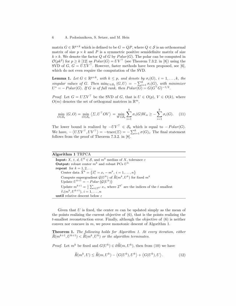
Algorithm 1 TRPCA
Input: X, t, d, U0 ∈ S, and m0 median of X, tolerance εOutput: robust center mk and robust PCs Uk
repeat for k = 1, 2, . . .Center data Xk =
{xki = xi −mk, i = 1, . . . , n
}Compute supergradient G(Uk) of R(mk, Uk) for fixed mk
Update Uk+1 = −Polar(G(Uk)
)Update mk+1 = 1
t
∑i∈Ik′ xi, where Ik
′are the indices of the t smallest
ri(mk, Uk+1), i = 1, . . . , n
until relative descent below ε
Given that U is fixed, the center m can be updated simply as the mean ofthe points realizing the current objective of (6), that is the points realizing thet-smallest reconstruction error. Finally, although the objective of (6) is neitherconvex nor concave in m, we prove monotonic descent of Algorithm 1.
Theorem 1. The following holds for Algorithm 1. At every iteration, eitherR(mk+1, Uk+1) < R(mk, Uk) or the algorithm terminates.
Proof. Let mk be fixed and G(Uk) ∈ ∂R(m,Uk), then from (10) we have
R(mk, U) ≤ R(m,Uk)−⟨G(Uk), Uk
⟩+⟨G(Uk), U
⟩. (12)

Robust PCA: Optimization of the Robust Reconstruction Error 7
The minimizer Uk+1 = arg minU∈Sk
⟨G(Uk), U
⟩, over the Stiefel manifold can be
computed via Lemma 1 as Uk+1 = −Polar(G(Uk)). Thus we get immediately,
R(mk, Uk+1) ≤ R(mk, Uk).
After the update of Uk+1 we compute Ik′ which are the indices of the t smallestri(m
k, Uk+1), i = 1, . . . , n. If there are ties, then they are broken randomly. Forfixed Uk+1 and fixed Ik′ the minimizer of the objective∑
i∈Ik′
−∥∥(Uk+1)>(xi −m)
∥∥22
+ ‖xi −m‖22 , (13)
is given bymk+1 = 1t
∑i∈Ik′
xi, which yields,∑i∈Ik′
ri(mk+1, Uk+1) ≤ R(mk, Uk+1).
After the computation of mk+1, Ik′ need no longer correspond to the t smallestreconstruction errors ri(m
k+1, Uk+1). However, taking the t smallest ones only
further reduces the objective, R(mk+1, Uk+1) ≤∑i∈Ik′ ri(m
k+1, Uk+1). This
yields finally the result, R(mk+1, Uk+1) ≤ R(mk, Uk).
The objective is non-smooth and neither convex nor concave. The Stiefelmanifold is a non-convex constraint set. These facts make the formulation ofcritical points conditions challenging. Thus, while potentially stronger conver-gence results like convergence to a critical point are appealing, they are currentlyout of reach. However, as we will see in Section 4, Algorithm 1 yields good empir-ical results, even beating state-of-the-art methods based on convex relaxationsor other non-convex formulations.
3.3 Complexity and Discussion
The computational cost of each iteration of Algorithm 1 is dominated by O(pk2)
for computing the polar and O(pkn) for a supergradient of R(m,U) and, thus,has total cost O(pk(k+n)). We compare this to the cost of the proximal methodin [3], [20] for minimizing minX=A+E ‖A‖∗+λ ‖E‖1. In each iteration, the dom-inating cost is O(min{pn2, np2}) for the SVD of a matrix of size p × n. If thenatural condition k � min{p, n} holds, we observe that the computational costof TRPCA is significantly better. Thus even though we do 10 random restartswith different starting vectors, our TRPCA is still faster than all competingmethods, which can also be seen from the runtimes in Table 1.
In [15], a relaxed version of the trimmed reconstruction error is minimized:
minm∈Rp, U∈Sk ,s∈Rk
∥∥X − 1nm> − Us−O
∥∥2F
+ λ ‖O‖2,1 , (14)
where ‖O‖2,1 is added in order to enforce row-wise sparsity of O. The opti-mization is done via an alternating scheme. However, the disadvantage of thisformulation is that it is difficult to adjust the number of outliers via the choiceof λ and thus requires multiple runs of the algorithm to find a suitable range,whereas in our formulation the number of outliers n−t can be directly controlledby the user or t can be set to the default value
⌈n2
⌉.
8 A. Podosinnikova, S. Setzer, and M. Hein
4 Experiments
We compare our TRPCA (the code is available for download at [18]) algorithmwith the following robust PCA methods: ORPCA [15], LLD2 [16], HRPCA [21],standard PCA, and true PCA on the true data T (ground truth). For backgroundsubtraction, we also compare our algorithm with PCP [3] and RPCA [19], al-though the latter two algorithms are developed for a different outlier model.
To get the best performance of LLD and ORPCA, we run both algorithmswith different values of the regularization parameters to set the number of zerorows (observations) in the outlier matrix equal to t (which increases runtimesignificantly). The HRPCA algorithm has the same parameter t as our method.
We write (0.5) in front of an algorithm name if the default value t =⌈n2
⌉is
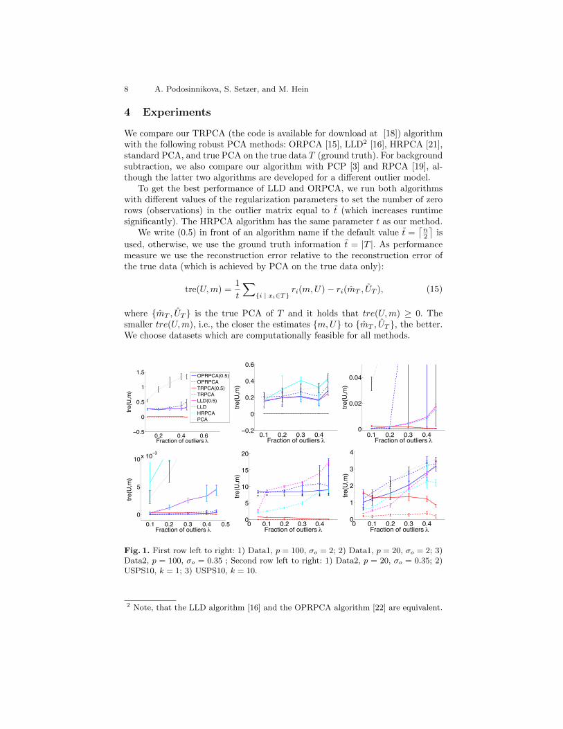
used, otherwise, we use the ground truth information t = |T |. As performancemeasure we use the reconstruction error relative to the reconstruction error ofthe true data (which is achieved by PCA on the true data only):
tre(U,m) =1
t
∑{i | xi∈T}
ri(m,U)− ri(mT , UT ), (15)
where {mT , UT } is the true PCA of T and it holds that tre(U,m) ≥ 0. Thesmaller tre(U,m), i.e., the closer the estimates {m,U} to {mT , UT }, the better.We choose datasets which are computationally feasible for all methods.
0.2 0.4 0.60.5
0
0.5
1
1.5
Fraction of outliers
tre(U
,m)
OPRPCA(0.5)OPRPCATRPCA(0.5)TRPCALLD(0.5)LLDHRPCAPCA
0.1 0.2 0.3 0.40.2
0
0.2
0.4
0.6
Fraction of outliers
tre(U
,m)
0.1 0.2 0.3 0.40
0.02
0.04
Fraction of outliers
tre(U
,m)
0.1 0.2 0.3 0.4 0.50
5
10x 10 3
Fraction of outliers
tre(U
,m)
0 0.1 0.2 0.3 0.40
5
10
15
20
Fraction of outliers
tre(U
,m)
0 0.1 0.2 0.3 0.40
1
2
3
4
Fraction of outliers
tre(U
,m)
Fig. 1. First row left to right: 1) Data1, p = 100, σo = 2; 2) Data1, p = 20, σo = 2; 3)Data2, p = 100, σo = 0.35 ; Second row left to right: 1) Data2, p = 20, σo = 0.35; 2)USPS10, k = 1; 3) USPS10, k = 10.
2 Note, that the LLD algorithm [16] and the OPRPCA algorithm [22] are equivalent.

Robust PCA: Optimization of the Robust Reconstruction Error 9
4.1 Synthetic Data Sets
We sample uniformly at random a subspace of dimension k spanned by U ∈ Skand generate the true data T ∈ Rt×p as T = AU> + E where the entries ofA ∈ Rt×k are sampled uniformly on [−1, 1] and the noise E ∈ Rt×p has Gaussianentries distributed as N (0, σT ). We consider two types of outliers: (Data1) theoutliers O ∈ Ro×p are uniform samples from [0, σo]
p, (Data2) the outliers aresamples from a random half-space, let w be sampled uniformly at random fromthe unit sphere and let x ∼ N (0, σ01) then an outlier oi ∈ Rp is generated asoi = x−max{〈x,w〉 , 0}w. For Data2, we also downscale true data by 0.5 factor.We always set n = t + o = 200, k = 5, and σT = 0.05 and construct data setsfor different fractions of outliers λ = o
t+o ∈ {0.1, 0.2, 0.3, 0.4, 0.45}. For every λwe sample 5 data sets and report mean and standard deviation of the relativetrue reconstruction error tre(U,m).
4.2 Partially Synthetic Data Set
We use USPS, a dataset of 16× 16 images of handwritten digits. We use digits1 as true observations T and digits 0 as outliers O and mix them in differentproportions. We refer to this data set as USPS10 and the results can be found inFig. 1. Another similar experiment is on the MNIST data set of 28× 28 imagesof handwritten digits. We use digits 1 (or 7) as true observations T and allother digits 0, 2, 3, . . . , 9 as outliers O (each taken in equal proportion). We mixtrue data and outliers in different proportions and the results can be found inFig. 2 (or Fig. 3), where we excluded LLD due to its low computational time,see Tab. 1. We notice that TRPCA algorithm with the parameter value t = t(ground truth information) performs almost perfectly and outperforms all othermethods, while the default version of TRPCA with parameter t =
⌈n2
⌉shows
slightly worse performance. The fact that TRPCA estimates simultaneously therobust center m influences positively the overall performance of the algorithm,see, e.g., the experiments for background subtraction and modeling in Section 4.3and additional ones in the supplementary material. That is Fig. 6-17.
4.3 Background Modeling and Subtraction
In [19] and [3] robust PCA has been proposed as a method for backgroundmodeling and subtraction. While we are not claiming that robust PCA is thebest method to do this, it is an interesting test for robust PCA. The data Xare the image frames of a video sequence. The idea is that slight change in thebackground leads to a low-rank variation of the data whereas the foregroundchanges cannot be modeled by this and can be considered as outliers. Thuswith the estimates m∗ and U∗ of the robust PCA methods, the solution of thebackground subtraction and modeling problem is given as
xbi = m∗ + U∗(U∗)>(xi −m∗) (16)
where xbi is the background of frame i and its foreground is simply xfi = xi−xbi .

10 A. Podosinnikova, S. Setzer, and M. Hein
0.2 0.4 0.60
2
4
6x 10
5
Fraction of outliers λ
tre
(U,m
)
PCA
OPRPCA(0.5)
OPRPCA
TRPCA(0.5)
TRPCA
HRPCA(0.5)
HRPCA
0.2 0.4 0.60
5
10
15x 10
5
Fraction of outliers λ
tre
(U,m
)
PCA
OPRPCA(0.5)
OPRPCA
TRPCA(0.5)
TRPCA
HRPCA(0.5)
HRPCA
Fig. 2. Experiment on the MNIST data set with digits 1 as true observations T andall other digits 0, 2, 3, . . . , 9 as outliers. Number of recovered PCs is k = 1 (left) andk = 5 (right).
0.2 0.4 0.60
5
10x 10
5
Fraction of outliers λ
tre
(U,m
)
PCA
OPRPCA(0.5)
OPRPCA
TRPCA(0.5)
TRPCA
HRPCA(0.5)
HRPCA
0.2 0.4 0.60
5
10
15x 10
5
Fraction of outliers λ
tre
(U,m
)
PCA
OPRPCA(0.5)
OPRPCA
TRPCA(0.5)
TRPCA
HRPCA(0.5)
HRPCA
Fig. 3. Experiment on the MNIST data set with digits 7 as true observations T andall other digits 0, 2, 3, . . . , 9 as outliers. Number of recovered PCs is k = 1 (left) andk = 5 (right).
0 200 400 6000
1
2x 10⁷
Observation/Frame i
Rec
. erro
r
True PCA
0 200 400 6000
1
2x 10⁷
Observation/Frame i
Rec
. erro
r
TRPCA
0 200 400 6000
1
2x 10⁷
Observation/Frame i
Rec
. erro
r
ORPCA
0 200 400 6000
1
2x 10⁷
Observation/Frame i
Rec
. erro
r
LLD
0 200 400 6000
1
2x 10⁷
Observation/Frame i
Rec
. erro
r
PCP =0.001
0 200 400 6000
1
2x 10⁷
Observation/Frame i
Rec
. erro
r
PCA
0 200 400 6000
1
2x 10⁷
Observation/Frame i
Rec
. erro
r
TRPCA(0.5)
0 200 400 6000
1
2x 10⁷
Observation/Frame i
Rec
. erro
r
HRPCA
0 200 400 6000
1
2x 10⁷
Observation/Frame i
Rec
. erro
r
RPCA
0 200 400 6000
1
2x 10⁷
Observation/Frame i
Rec
. erro
r
PCP =0.009
Fig. 4. Reconstruction errors, i.e., ||(xi −m∗)− U∗ (U∗)> (xi −m∗)||22, on the y-axis,for each frame on the x-axes for k = 10. Note that the person is visible in the scenefrom frame 481 until the end. We consider the background images as true data and,thus, the reconstruction error should be high after frame 481 (when the person enters).
Robust PCA: Optimization of the Robust Reconstruction Error 11
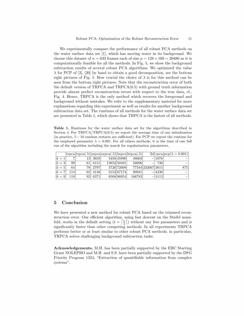
We experimentally compare the performance of all robust PCA methods onthe water surface data set [1], which has moving water in its background. Wechoose this dataset of n = 633 frames each of size p = 128× 160 = 20480 as it iscomputationally feasible for all the methods. In Fig. 5, we show the backgroundsubtraction results of several robust PCA algorithms. We optimized the valueλ for PCP of [3], [20] by hand to obtain a good decomposition, see the bottomright pictures of Fig. 5. How crucial the choice of λ is for this method can beseen from the bottom right pictures. Note that the reconstruction error of boththe default version of TRPCA and TRPCA(0.5) with ground truth informationprovide almost perfect reconstruction errors with respect to the true data, cf.,Fig. 4. Hence, TRPCA is the only method which recovers the foreground andbackground without mistakes. We refer to the supplementary material for moreexplanations regarding this experiment as well as results for another backgroundsubtraction data set. The runtimes of all methods for the water surface data setare presented in Table 1, which shows that TRPCA is the fastest of all methods.
Table 1. Runtimes for the water surface data set for the algorithms described inSection 4. For TRPCA/TRPCA(0.5) we report the average time of one initialization(in practice, 5− 10 random restarts are sufficient). For PCP we report the runtime forthe employed parameter λ = 0.001. For all others methods, it is the time of one fullrun of the algorithm including the search for regularization parameters.
trpca trpca(.5) orpca orpca(.5) hrpca hrpca(.5) lld rpca pcp(λ = 0.001)
k = 1 7 13 3659 3450 45990 48603 − 1078 −k = 3 99 61 8151 13852 50491 56090 − 730 −k = 5 64 78 2797 3726 72009 77344 232667 3615 875
k = 7 114 62 4138 3153 67174 90931 − 4230 −k = 9 119 92 6371 8508 96954 106782 − 4113 −
5 Conclusion
We have presented a new method for robust PCA based on the trimmed recon-struction error. Our efficient algorithm, using fast descent on the Stiefel mani-fold, works in the default setting (t =
⌈n2
⌉) without any free parameters and is
significantly faster than other competing methods. In all experiments TRPCAperforms better or at least similar to other robust PCA methods, in particular,TRPCA solves challenging background subtraction tasks.
Acknowledgements. M.H. has been partially supported by the ERC StartingGrant NOLEPRO and M.H. and S.S. have been partially supported by the DFGPriority Program 1324, “Extraction of quantifiable information from complexsystems”.

12 A. Podosinnikova, S. Setzer, and M. Hein
0 100 2000
50
100
150Background i = 560, PCA
50
100
150
200
0 100 2000
50
100
150Foreground i = 560, PCA
−50
0
50
100
0 100 2000
50
100
150Background i = 560, true PCA
50
100
150
0 100 2000
50
100
150Foreground i = 560, true PCA
−100
−50
0
50
0 100 2000
50
100
150Background i = 560, TRPCA
50
100
150
0 100 2000
50
100
150Foreground i = 560, TRPCA
−100
−50
0
50
0 100 2000
50
100
150Background i = 560, TRPCA(0.5)
50
100
150
0 100 2000
50
100
150Foreground i = 560, TRPCA(0.5)
−100
−50
0
0 100 2000
50
100
150Background i = 560, ORPCA
50
100
150
200
0 100 2000
50
100
150Foreground i = 560, ORPCA
−50
0
50
100
0 100 2000
50
100
150Background i = 560, HRPCA
50
100
150
0 100 2000
50
100
150Foreground i = 560, HRPCA
−100
−50
0
50
100
0 100 2000
50
100
150Background i = 560, LLD
50
100
150
0 100 2000
50
100
150Foreground i = 560, LLD
−100
−50
0
50
100
0 100 2000
50
100
150Background i = 560, RPCA
−100
0
100
200
0 100 2000
50
100
150Foreground i = 560, RPCA
−100
0
100
200
0 100 2000
50
100
150Background, λ = 0.009, i = 560
50
100
150
0 100 2000
50
100
150Foreground, λ = 0.009, i = 560
−100
−50
0
50
100
0 100 2000
50
100
150Background, λ = 0.001, i = 560
50
100
150
0 100 2000
50
100
150Foreground, λ = 0.001, i = 560
−100
−50
0
Fig. 5. Backgrounds and foreground for frame i = 560 of the water surface data set.The last row corresponds to the PCP algorithm with values of λ set by hand
Robust PCA: Optimization of the Robust Reconstruction Error 13
References
1. Bouwmans, T.: Recent advanced statistical background modeling for foregrounddetection: A systematic survey. Recent Patents on Computer Science 4(3), 147–176(2011)
2. Boyd, S., Vandenberghe, L.: Convex Optimization. Cambridge University Press,Cambridge (2004)
3. Candes, E., Li, X., Ma, Y., Wright, J.: Robust principal component analysis? Jour-nal of the ACM 58(3) (2011)
4. Croux, C., Pilzmoser, P., Oliveira, M.R.: Algorithms for projection–pursuit robustprincipal component analysis. Chemometrics and Intelligent Laboratory Systems87, 218–225 (2007)
5. Hampel, F.R., Ronchetti, E.M., Rousseeuw, P.J., Stahel, W.A.: Robust Statistics.The Approach Based on Influence Functions. John Wiley and Sons, New York(1986)
6. Higham, N.J., Schreiber, R.S.: Fast polar decomposition of an arbitrary matrix.SIAM Journal on Scientific Computing 11(4), 648–655 (1990)
7. Hiriart-Urruty, J.B., Lemarechal: Fundamentals of Convex Analysis. Springer,Berlin (2001)
8. Horn, R., Johnson, C.: Matrix Analysis. Cambridge University Press, Cambridge(1990)
9. Huber, P.J.: Projection pursuit. Annals of Statistics 13(2), 435–475 (1985)
10. Huber, P., Ronchetti, E.: Robust Statistics. John Wiley and Sons, New York, 2ndedn. (2009)
11. Jolliffe, I.: Principal Component Analysis. Springer, New York, 2nd edn. (2002)
12. Journee, M., Nesterov, Y., Richtarik, P., Sepulchre, R.: Generalized power methodfor sparse principal component analysis. Journal of Machine Learning Research1(1), 517–553 (2010)
13. Li, G., Chen, Z.: Projection–pursuit approach to robust dispersion matrices andprincipal components: Primary theory and Monte Carlo. Journal of the AmericanStatistical Association 80(391), 759–766 (1985)
14. Mackey, L.: Deflation methods for sparse PCA. In: 24th Conference on NeuralInformation Processing Systems. pp. 1017–1024 (2009)
15. Mateos, G., Giannakis, G.: Robust PCA as bilinear decomposition with outlier-sparsity regularization. IEEE Transactions on Signal Processing 60(10), 5176–5190(2012)
16. McCoy, M., Tropp, J.A.: Two proposals for robust PCA using semidefinite pro-gramming. Electronic Journal of Statistics 5, 1123–1160 (2011)
17. Rousseeuw, P.J.: Least median of squares regression. Journal of the AmericanStatistical Association 79(388), 871–880 (1984)
18. Supplementary material. http://www.ml.uni-saarland.de/code/trpca/trpca.html
19. De la Torre, F., Black, M.: Robust principal component analysis for computervision. In: 8th IEEE International Conference on Computer Vision. pp. 362–369(2001)
20. Wright, J., Peng, Y., Ma, Y., Ganesh, A., Rao, S.: Robust principal componentanalysis: Exact recovery of corrupted low-rank matrices by convex optimization. In:24th Conference on Neural Information Processing Systems. pp. 2080–2088 (2009)
21. Xu, H., Caramanis, C., Mannor, S.: Outlier-robust PCA: the high dimensionalcase. IEEE Transactions on Information Theory 59(1), 546–572 (2013)
14 A. Podosinnikova, S. Setzer, and M. Hein
22. Xu, H., Caramanis, C., Sanghavi, S.: Robust PCA via outlier pursuit. IEEE Trans-actions on Information Theory 58(5), 3047–3064 (2012)
23. Xu, L., Yuille, A.L.: Robust principal component analysis by self-organizing rulesbased on statistical physics approach. IEEE Transactions on Neural Networks 6,131–143 (1995)
Robust PCA: Optimization of the Robust Reconstruction Error 15
6 Supplementary material: Experiments
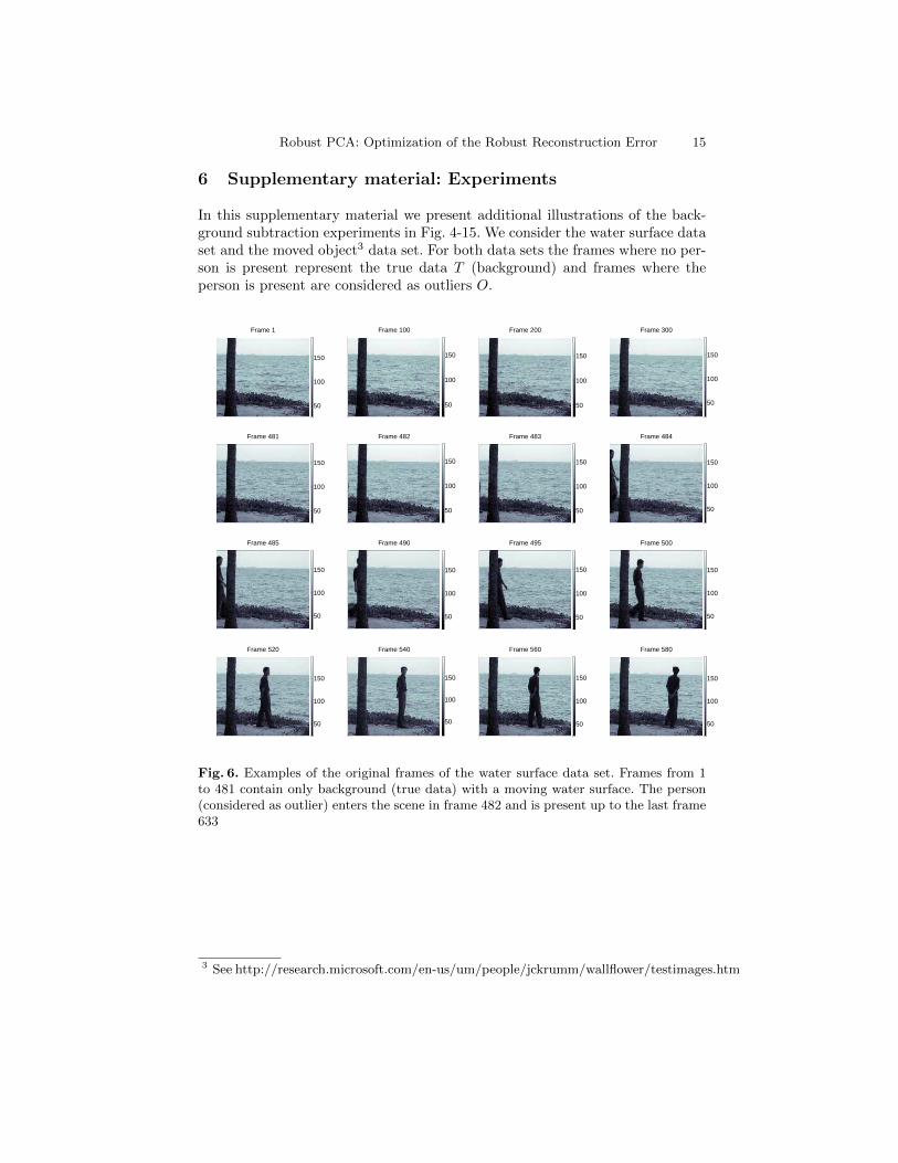
In this supplementary material we present additional illustrations of the back-ground subtraction experiments in Fig. 4-15. We consider the water surface dataset and the moved object3 data set. For both data sets the frames where no per-son is present represent the true data T (background) and frames where theperson is present are considered as outliers O.
Frame 1
50
100
150
Frame 100
50
100
150
Frame 200
50
100
150
Frame 300
50
100
150
Frame 481
50
100
150
Frame 482
50
100
150
Frame 483
50
100
150
Frame 484
50
100
150
Frame 485
50
100
150
Frame 490
50
100
150
Frame 495
50
100
150
Frame 500
50
100
150
Frame 520
50
100
150
Frame 540
50
100
150
Frame 560
50
100
150
Frame 580
50
100
150
Fig. 6. Examples of the original frames of the water surface data set. Frames from 1to 481 contain only background (true data) with a moving water surface. The person(considered as outlier) enters the scene in frame 482 and is present up to the last frame633
3 See http://research.microsoft.com/en-us/um/people/jckrumm/wallflower/testimages.htm
16 A. Podosinnikova, S. Setzer, and M. Hein
Background, frame 560, PCA (on X)
0
50
100
150Foreground, frame 560, PCA (on X)
−50
0
50Background, frame 560, True PCA (on T)
0
50
100
150Foreground, frame 560, True PCA (on T)
−50
0
50
Background, frame 560, TRPCA(0.5)
0
50
100
150Foreground, frame 560, TRPCA(0.5)
−50
0
50Background, frame 560, TRPCA
0
50
100
150Foreground, frame 560, TRPCA
−50
0
50
Background, frame 560, ORPCA
0
50
100
150Foreground, frame 560, ORPCA
−50
0
50Background, frame 560, HRPCA
0
50
100
150Foreground, frame 560, HRPCA
−50
0
50
Background, frame 560, LLD
0
50
100
150Foreground, frame 560, LLD
−50
0
50Background, frame 560, RPCA
0
50
100
150Foreground, frame 560, RPCA
−50
0
50
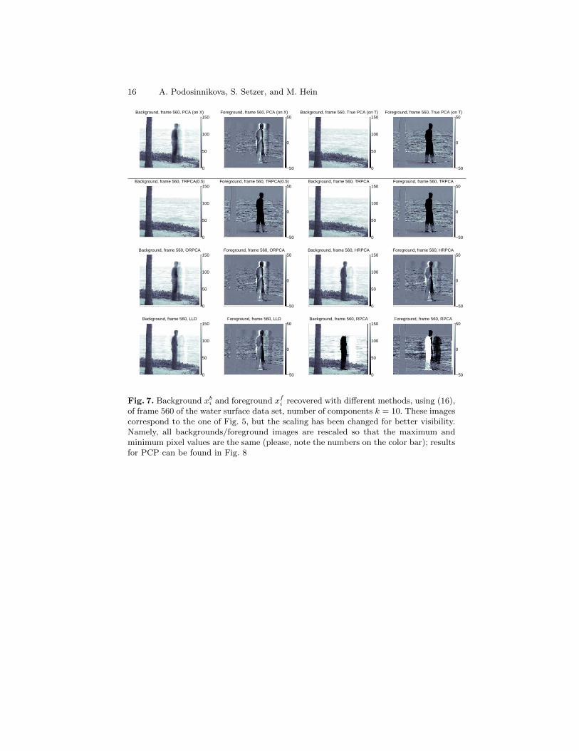
Fig. 7. Background xbi and foreground xfi recovered with different methods, using (16),of frame 560 of the water surface data set, number of components k = 10. These imagescorrespond to the one of Fig. 5, but the scaling has been changed for better visibility.Namely, all backgrounds/foreground images are rescaled so that the maximum andminimum pixel values are the same (please, note the numbers on the color bar); resultsfor PCP can be found in Fig. 8
Robust PCA: Optimization of the Robust Reconstruction Error 17
Background, frame 560, PCP (λ=0.0001)
0
50
100
150Foreground, frame 560, PCP (λ=0.0001)
−50
0
50Background, frame 560, PCP (λ=0.001)
0
50
100
150Foreground, frame 560, PCP (λ=0.001)
−50
0
50
Background, frame 560, PCP (λ=0.005)
0
50
100
150Foreground, frame 560, PCP (λ=0.005)
−50
0
50Background, frame 560, PCP (λ=0.006)
0
50
100
150Foreground, frame 560, PCP (λ=0.006)
−50
0
50
Background, frame 560, PCP (λ=0.007)
0
50
100
150Foreground, frame 560, PCP (λ=0.007)
−50
0
50Background, frame 560, PCP (λ=0.009)
0
50
100
150Foreground, frame 560, PCP (λ=0.009)
−50
0
50
Background, frame 560, PCP (λ=0.05)
0
50
100
150Foreground, frame 560, PCP (λ=0.05)
−50
0
50Background, frame 560, PCP (λ=0.1)
0
50
100
150Foreground, frame 560, PCP (λ=0.1)
−50
0
50
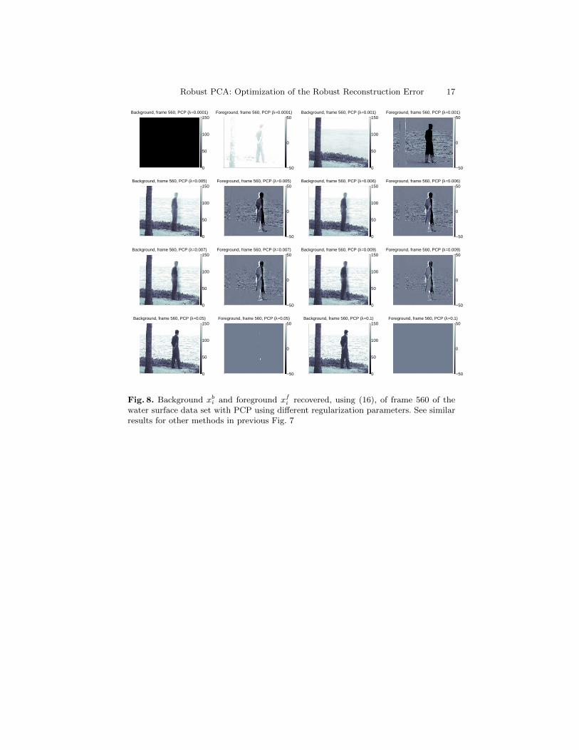
Fig. 8. Background xbi and foreground xfi recovered, using (16), of frame 560 of thewater surface data set with PCP using different regularization parameters. See similarresults for other methods in previous Fig. 7
18 A. Podosinnikova, S. Setzer, and M. Hein
Frame 1
0
100
200
Frame 500
0
100
200
Frame 600
0
100
200
Frame 637
0
100
200
Frame 638
0
100
200
Frame 639
0
100
200
Frame 650
0
100
200
Frame 660
0
100
200
Frame 670
0
100
200
Frame 700
0
100
200
Frame 750
0
100
200
Frame 800
0
100
200
Frame 890
0
100
200
Frame 1000
0
100
200
Frame 1100
0
100
200
Frame 1300
0
100
200
Frame 1389
0
100
200
Frame 1390
0
100
200
Frame 1391
0
100
200
Frame 1400
0
100
200
Frame 1420
0
100
200
Frame 1440
0
100
200
Frame 1460
0
100
200
Frame 1500
0
100
200
Frame 1501
0
100
200
Frame 1502
0
100
200
Frame 1600
0
100
200
Frame 1700
0
100
200
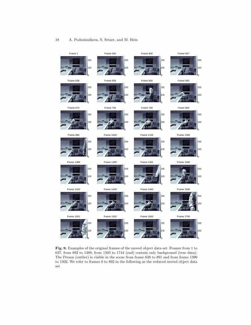
Fig. 9. Examples of the original frames of the moved object data set. Frames from 1 to637, from 892 to 1389, from 1503 to 1744 (end) contain only background (true data).The Person (outlier) is visible in the scene from frame 638 to 891 and from frame 1390to 1502. We refer to frames 0 to 892 in the following as the reduced moved object dataset

Robust PCA: Optimization of the Robust Reconstruction Error 19
0 500 1000 15000
1
2
3x 10⁷
Observation/frame i
Rec
. erro
r
TRPCA(0.5)
0 500 1000 15000
1
2
3x 10⁷
Observation/frame i
Rec
. erro
r
TRPCA
Fig. 10. The reconstruction error of TPRCA/TRPCA(0.5), by analogy with Fig. 4, forthe full moved object data set. The red vertical lines correspond to frames where theperson enters/leaves the scene. We do not perform this experiment on the full datsetfor all other methods given their high runtimes (see Table 1) and instead proceed withthe reduced dataset (see figures below).Please note also that there is a small change in the background between frames from1 to 637 (B1) and frames from 892 to 1389 (B2). Thus the robust PCA componentswill capture this difference. This is not a problem for outlier detection (as we cansee from the reconstruction errors of our method above) as this change is still smallcompared to the variation when the person enters the scene but it disturbs the fore-ground/background detection of all methods. An offline method could detect the sceneswith small reconstruction error and do the background/foreground decomposition foreach segment separately. The other option would be to use an online estimation proce-dure of robust components and center. We do not pursue these directions in this paperas the main purpose of these experiments is an illustration of the differences of thevarious robust PCA methods in the literature
20 A. Podosinnikova, S. Setzer, and M. Hein
Background, frame 651, PCA (on X)
−200
−100
0
100
200Foreground, frame 651, PCA (on X)
−200
−100
0
100
200Background, frame 651, True PCA (on T)
−200
−100
0
100
200Foreground, frame 651, True PCA (on T)
−200
−100
0
100
200
Background, frame 651, TRPCA(0.5)
−200
−100
0
100
200Foreground, frame 651, TRPCA(0.5)
−200
−100
0
100
200Background, frame 651, TRPCA
−200
−100
0
100
200Foreground, frame 651, TRPCA
−200
−100
0
100
200
Background, frame 651, ORPCA
−200
−100
0
100
200Foreground, frame 651, ORPCA
−200
−100
0
100
200Background, frame 651, HRPCA
−200
−100
0
100
200Foreground, frame 651, HRPCA
−200
−100
0
100
200
Background, frame 651, LLD
−200
−100
0
100
200Foreground, frame 651, LLD
−200
−100
0
100
200Background, frame 651, RPCA
−200
−100
0
100
200Foreground, frame 651, RPCA
−200
−100
0
100
200
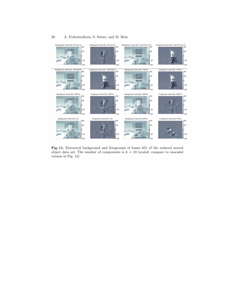
Fig. 11. Extracted background and foreground of frame 651 of the reduced movedobject data set. The number of components is k = 10 (scaled, compare to unscaledversion in Fig. 12)
Robust PCA: Optimization of the Robust Reconstruction Error 21
Background, frame 651, PCA (on X)
50
100
150
200
Foreground, frame 651, PCA (on X)
−150
−100
−50
0
50
100
Background, frame 651, True PCA (on T)
−100
0
100
200
Foreground, frame 651, True PCA (on T)
−100
0
100
200
Background, frame 651, TRPCA(0.5)
0
50
100
150
200
250Foreground, frame 651, TRPCA(0.5)
−100
0
100
200
Background, frame 651, TRPCA
−100
0
100
200
Foreground, frame 651, TRPCA
−100
0
100
200
Background, frame 651, ORPCA
0
50
100
150
200
Foreground, frame 651, ORPCA
−100
−50
0
50
100
150
Background, frame 651, HRPCA
0
50
100
150
200
250
Foreground, frame 651, HRPCA
−100
−50
0
50
100
Background, frame 651, LLD
0
100
200
300
Foreground, frame 651, LLD
−150
−100
−50
0
50
100
Background, frame 651, RPCA
−100
0
100
200
300
Foreground, frame 651, RPCA
−200
−100
0
100
200
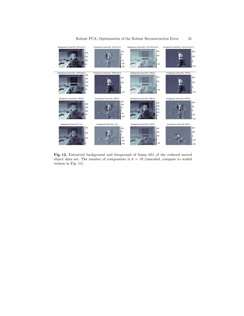
Fig. 12. Extracted background and foreground of frame 651 of the reduced movedobject data set. The number of components is k = 10 (unscaled, compare to scaledversion in Fig. 11)
22 A. Podosinnikova, S. Setzer, and M. Hein
Background, frame 681, PCA (on X)
−200
−100
0
100
200Foreground, frame 681, PCA (on X)
−200
−100
0
100
200Background, frame 681, True PCA (on T)
−200
−100
0
100
200Foreground, frame 681, True PCA (on T)
−200
−100
0
100
200
Background, frame 681, TRPCA(0.5)
−200
−100
0
100
200Foreground, frame 681, TRPCA(0.5)
−200
−100
0
100
200Background, frame 681, TRPCA
−200
−100
0
100
200Foreground, frame 681, TRPCA
−200
−100
0
100
200
Background, frame 681, ORPCA
−200
−100
0
100
200Foreground, frame 681, ORPCA
−200
−100
0
100
200Background, frame 681, HRPCA
−200
−100
0
100
200Foreground, frame 681, HRPCA
−200
−100
0
100
200
Background, frame 681, LLD
−200
−100
0
100
200Foreground, frame 681, LLD
−200
−100
0
100
200Background, frame 681, RPCA
−200
−100
0
100
200Foreground, frame 681, RPCA
−200
−100
0
100
200
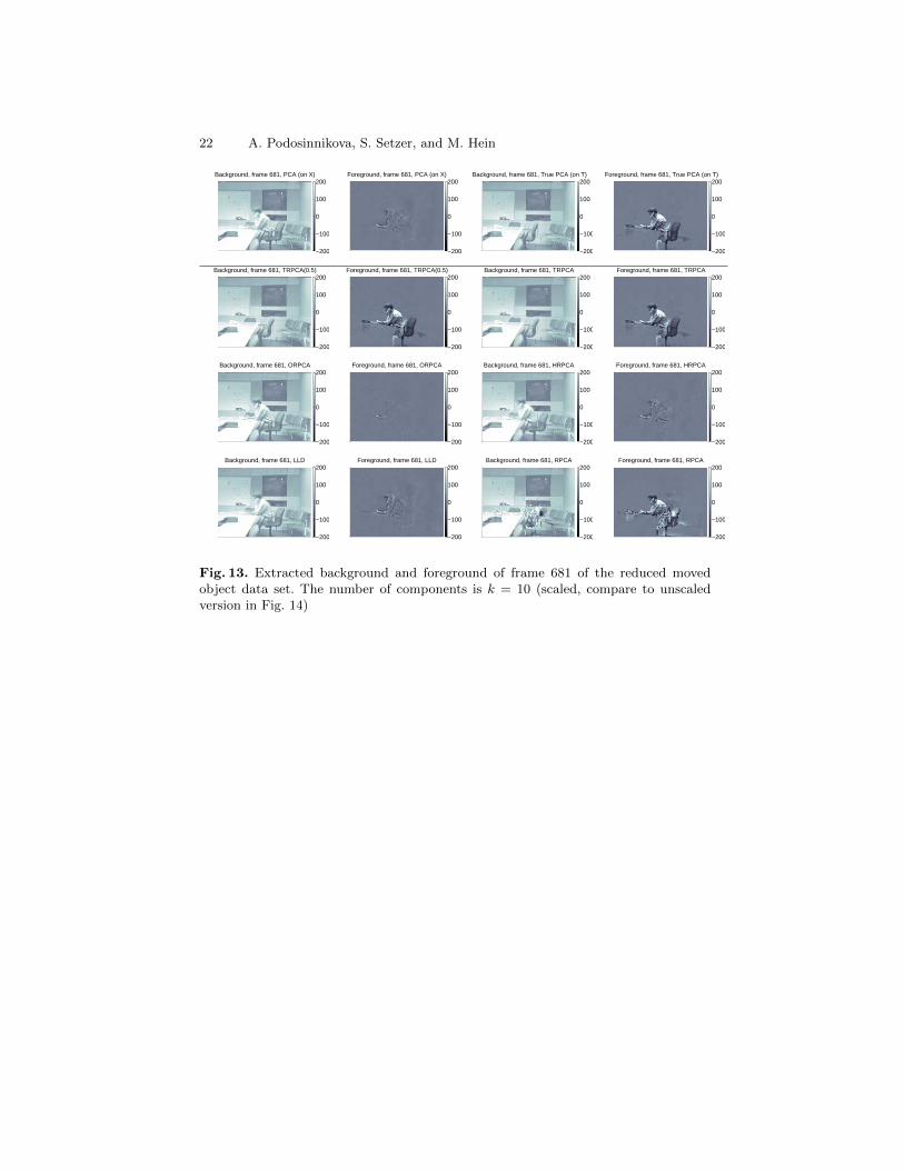
Fig. 13. Extracted background and foreground of frame 681 of the reduced movedobject data set. The number of components is k = 10 (scaled, compare to unscaledversion in Fig. 14)

Robust PCA: Optimization of the Robust Reconstruction Error 23
Background, frame 681, PCA (on X)
0
50
100
150
200
250
Foreground, frame 681, PCA (on X)
−100
−50
0
50
100
Background, frame 681, True PCA (on T)
0
50
100
150
200
250Foreground, frame 681, True PCA (on T)
−100
0
100
200
Background, frame 681, TRPCA(0.5)
0
50
100
150
200
250Foreground, frame 681, TRPCA(0.5)
−100
0
100
200
Background, frame 681, TRPCA
0
50
100
150
200
250Foreground, frame 681, TRPCA
−100
0
100
200
Background, frame 681, ORPCA
0
50
100
150
200
250
Foreground, frame 681, ORPCA
−100
−50
0
50
100
Background, frame 681, HRPCA
0
50
100
150
200
250
Foreground, frame 681, HRPCA
−100
−50
0
50
100
Background, frame 681, LLD
0
50
100
150
200
250
Foreground, frame 681, LLD
−100
−50
0
50
100
Background, frame 681, RPCA
−100
0
100
200
300
Foreground, frame 681, RPCA
−200
−100
0
100
200
Fig. 14. Extracted background and foreground of frame 681 of the reduced movedobject data set. The number of components is k = 10 (unscaled, compare to scaledversion in Fig. 13)

24 A. Podosinnikova, S. Setzer, and M. Hein
Background, frame 651, PCP (λ=0.0005)
0
50
100
150Foreground, frame 651, PCP (λ=0.0005)
−50
0
50Background, frame 651, PCP (λ=0.001)
0
50
100
150Foreground, frame 651, PCP (λ=0.001)
−50
0
50
Background, frame 651, PCP (λ=0.005)
0
50
100
150Foreground, frame 651, PCP (λ=0.005)
−50
0
50Background, frame 681, PCP (λ=0.0005)
0
50
100
150Foreground, frame 681, PCP (λ=0.0005)
−50
0
50
Background, frame 681, PCP (λ=0.001)
0
50
100
150Foreground, frame 681, PCP (λ=0.001)
−50
0
50Background, frame 681, PCP (λ=0.005)
0
50
100
150Foreground, frame 681, PCP (λ=0.005)
−50
0
50
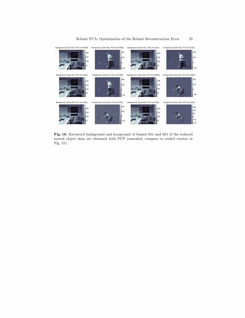
Fig. 15. Extracted background and foreground of frames 651 and 681 of the reducedmoved object data set obtained with PCP (scaled, compare to unscaled version inFig. 16)
Robust PCA: Optimization of the Robust Reconstruction Error 25
Background, frame 651, PCP (λ=0.0005)
50
100
150
200
Foreground, frame 651, PCP (λ=0.0005)
−100
0
100
200
Background, frame 651, PCP (λ=0.001)
50
100
150
200
Foreground, frame 651, PCP (λ=0.001)
−100
0
100
200
Background, frame 651, PCP (λ=0.005)
50
100
150
200
Foreground, frame 651, PCP (λ=0.005)
−100
0
100
200
Background, frame 681, PCP (λ=0.0005)
50
100
150
200
Foreground, frame 681, PCP (λ=0.0005)
−100
0
100
200
Background, frame 681, PCP (λ=0.001)
50
100
150
200
Foreground, frame 681, PCP (λ=0.001)
−100
0
100
200
Background, frame 681, PCP (λ=0.005)
50
100
150
200
Foreground, frame 681, PCP (λ=0.005)
−100
−50
0
50
100
150
Fig. 16. Extracted background and foreground of frames 651 and 681 of the reducedmoved object data set obtained with PCP (unscaled, compare to scaled version inFig. 15)
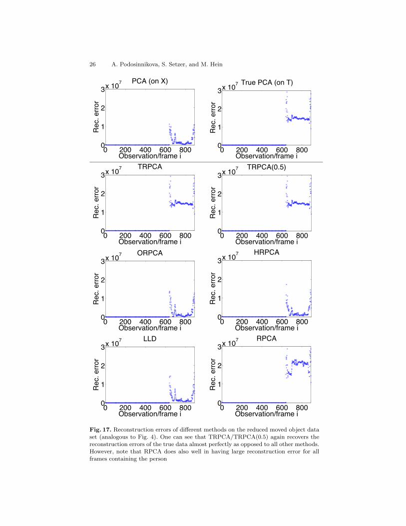
26 A. Podosinnikova, S. Setzer, and M. Hein
0 200 400 600 8000
1
2
3x 10⁷
Rec
. erro
r
Observation/frame i
PCA (on X)
0 200 400 600 8000
1
2
3x 10⁷
Rec
. erro
r
Observation/frame i
True PCA (on T)
0 200 400 600 8000
1
2
3x 10⁷
Rec
. erro
r
Observation/frame i
TRPCA
0 200 400 600 8000
1
2
3x 10⁷
Observation/frame i
Rec
. erro
r
TRPCA(0.5)
0 200 400 600 8000
1
2
3x 10⁷
Rec
. erro
r
Observation/frame i
ORPCA
0 200 400 600 8000
1
2
3x 10⁷
Rec
. erro
r
Observation/frame i
HRPCA
0 200 400 600 8000
1
2
3x 10⁷
Rec
. erro
r
Observation/frame i
LLD
0 200 400 600 8000
1
2
3x 10⁷
Rec
. erro
r
Observation/frame i
RPCA
Fig. 17. Reconstruction errors of different methods on the reduced moved object dataset (analogous to Fig. 4). One can see that TRPCA/TRPCA(0.5) again recovers thereconstruction errors of the true data almost perfectly as opposed to all other methods.However, note that RPCA does also well in having large reconstruction error for allframes containing the person