* Corresponding author: sankaran.mahadevan@vanderbilt.edu

Robustness-based Design Optimization under Data Uncertainty

Kais Zaman, Mark McDonald, Sankaran Mahadevan*

Vanderbilt University, Nashville, TN, USA and Lawrence Green

NASA Langley Research Center, Hampton, Virginia

Abstract

This paper proposes formulations and algorithms for design optimization under both aleatory (i.e., natural or physical variability) and epistemic uncertainty (i.e., imprecise probabilistic information), from the perspective of system robustness. The proposed formulations deal with epistemic uncertainty arising from both sparse and interval data without any assumption about the probability distributions of the random variables. A decoupled approach is proposed in this paper to un-nest the robustness-based design from the analysis of non-design epistemic variables to achieve computational efficiency. The proposed methods are illustrated for the upper stage design problem of a two-stage-to-orbit (TSTO) vehicle, where the information on the random design inputs are only available as sparse point and/or interval data. As collecting more data reduces uncertainty but increases cost, the effect of sample size on the optimality and robustness of the solution is also studied. A method is developed to determine the optimal sample size for sparse point data that leads to the solutions of the design problem that are least sensitive to variations in the input random variables.

1. Introduction

In deterministic design optimization, it is generally assumed that all design variables

and system variables are precisely known; the influence of natural variability and data

uncertainty on the optimality and feasibility of the design is not explicitly considered.

However, real-life engineering problems are non-deterministic, and a deterministic

assumption about inputs may lead to infeasibility or poor performance (Sim, 2006). In

recent years, many methods have been developed for design under uncertainty.

Reliability-based design (e.g., Chiralaksanakul and Mahadevan, 2005; Ramu et al, 2006;

Agarwal et al, 2007and Du and Huang, 2007) and robust design (e.g., Parkinson et al,

https://ntrs.nasa.gov/search.jsp?R=20110016346 2018-08-14T18:49:40+00:00Z

2

1993; Du and Chen, 2000; Doltsinis and Kang, 2004 and Huang and Du, 2007) are two

directions pursued by these methods. While reliability-based design aims to maintain

design feasibility at desired reliability levels, robust design optimization attempts to

minimize variability in the system performance due to variations in the inputs (Lee et al,

2008). In recent years, several methods have also been proposed to integrate these two

paradigms of design under uncertainty (e.g., Du et al, 2004, Lee et al, 2008).

Taguchi proposed robust design methods for selecting design variables in a manner

that makes the product performance insensitive to variations in the manufacturing process

(Taguchi, 1993). Taguchi’s methods have widespread applications in engineering;

however, these methods are implemented through statistical design of experiments and

cannot solve problems with multiple measures of performances and design constraints

(Wei et al, 2009). With the introduction of nonlinear programming to robust design, it has

become possible to achieve robustness in both performance and design constraints (Du

and Chen, 2000).

The essential elements of robust design optimization are: (1) maintaining robustness

in the objective function (objective robustness); (2) maintaining robustness in the

constraints (feasibility robustness); (3) estimating mean and measure of variation

(variance) of the performance function; and (4) multi-objective optimization. The rest of

this section briefly reviews the literature with respect to these four elements and

establishes the motivation for the current study.

Objective robustness

In robust optimization, the robustness of the objective function is usually achieved by

simultaneously optimizing its mean and minimizing its variance. Two major robustness

3

measures are available in the literature: one is the variance, which is extensively

discussed in the literature (Du and Chen, 2000; Lee and Park, 2001 and Doltsinis and

Kang, 2004) and the other is based on the percentile difference (Du et al, 2004). Although

the percentile difference method has the advantage that it contains the information of

probability in the tail regions of the performance distribution, this method is only

applicable to unimodal distributions. Variance as a measure of variation of the

performance function can be applied to any distribution (unimodal or multimodal), but it

only characterizes the dispersion around the mean (Huang and Du, 2007).

Feasibility robustness

Feasibility robustness i.e., robustness in the constraints can be defined as satisfying

the constraints of the design in the presence of uncertainty. Du and Chen (2000)

classified the methods of maintaining feasibility robustness into two categories, methods

that use probabilistic and statistical analysis, and methods that do not require them.

Among the methods that require probabilistic and statistical analysis, a probabilistic

feasibility formulation (Du and Chen, 2000 and Lee et al, 2008), and a moment matching

formulation (Parkinson et al, 1993) have been proposed. Du and Chen (2000) used a most

probable point (MPP)-based importance sampling method to reduce the computational

burden associated with the probabilistic feasibility formulation. The moment matching

formulation is a simplified approach which requires only the constraints on the first and

second moments of the performance function to be satisfied, and assumes that the

performance function is normally distributed. A variation of this approach, the feasible

region reduction method has been described in Park et al (2006), which is more general

and does not require the normality assumption. This is a tolerance design method, where

4

width of the feasible space in each direction is reduced by the amount k , where k is a

user-defined constant and is the standard deviation of the performance function. This

method only requires the mean and variance of the performance function.

Methods that do not require probabilistic and statistical analysis are also available, for

example, worst case analysis (Parkinson et al, 1993), corner space evaluation

(Sundaresan et al, 1995), and manufacturing variation patterns (MVP) (Yu and Ishii,

1998). A comparison study of the different constraint feasibility methods can be found in

Du and Chen (2000).

Estimating mean and variance of the performance function

Various methods have been reported in the literature to estimate the mean and

standard deviation of the performance function. These methods can be divided into three

major classes: (i) Taylor series expansion methods, (ii) sampling-based methods and (iii)

point estimate methods (Huang and Du, 2007).

The Taylor series expansion method (Haldar and Mahadevan, 2000; Du and Chen,

2000; and Lee et al, 2001) is a simple approach. However, for a nonlinear performance

function, if the variances of the random variables are large, this approximation may result

in large errors (Du et al., 2004). Although a second-order Taylor series expansion is

generally more accurate than the first-order approximation, it is also computationally

more expensive.

Sampling-based methods require information on distributions of the random

variables, and are expensive. Efficient sampling techniques such as importance sampling,

Latin hypercube sampling, etc. (Robert and Cesalla, 2004) can be used to reduce the

computational effort, but are still prohibitive in the context of optimization. Surrogate

5

models (Ghanem and Spanos 1991; Bichon et al, 2008; Cheng and Sandu, 2009) may be

used to further reduce computational effort.

In an attempt to overcome the difficulties associated with the computation of

derivatives required in Taylor series expansion, Rosenlblueth (1975) proposed a point

estimate method to compute the first few moments of the performance function. Different

variations of this point estimate method (Hong, 1998; Zhao and Ono, 2000 and Zhao and

Ang, 2003) have been studied. Although point estimate methods are easier to implement,

the accuracy may be low and may generate points that lie outside the domain of the

random variable.

Multi-objective optimization

Robustness-based optimization considers two objectives: optimize the mean of the

objective function and minimize its variation. An extensive survey of the multi-objective

optimization methods can be found in Marler and Arora (2004). Among the available

methods, the weighted sum approach is the most common approach to multi-objective

optimization and has been extensively used in robust design optimization (Lee and Park,

2001; Doltsinis and Kang, 2004; Zou and Mahadevan, 2006). The designer can obtain

alternative design points by varying the weights and can select the one that offers the best

trade-off among multiple objectives. Despite its simplicity, the weighted sum method

may not obtain potentially desirable solutions (Park et al, 2006). Another common

approach is the ε-constraint method in which one of the objective functions is optimized

while the other objective functions are used as constraints. Despite its advantages over

weighted sum method in some cases, the ε-constraint method can be computationally

expensive for more than two objective functions (Mavrotas, 2009).

6

Other methods include goal programming (Zou and Mahadevan, 2006), compromise

decision support problem (Bras and Mistree, 1993, 1995; Chen et al, 1996), compromise

programming (CP) (Zalney, 1973; Zhang, 2003; Chen et al, 1999) and physical

programming (Messac, 1996; Messac et al, 2001; Messac and Ismail-Yahaya, 2002; Chen

et al, 2000). Each of these methods has its own advantages and limitations.

Although there is now an extensive volume of literature for robust optimization

methods and applications, all these methods have only been studied with respect to

physical or natural variability represented by probability distributions. Uncertainty in

system design also arises from other contributing factors. Sources of uncertainty may be

divided into two types: aleatory and epistemic (Oberkampf et. al., 2004). Aleatory

uncertainty is irreducible. Examples include phenomena that exhibit natural variation like

operating conditions, material properties, geometric tolerances, etc. In contrast, epistemic

uncertainty results from a lack of knowledge about the system, or due to approximations

in the system behavior models, or due to limited or subjective (e.g., expert opinion) data;

it can be reduced as more information about the system is obtained.

One type of data uncertainty involves having limited data to properly define the

distribution parameters of the random variables. This type of uncertainty may be reduced

by collecting more data. In some cases of data uncertainty, distribution information of a

random variable may only be available as intervals given by experts. The objective of this

paper is to develop an efficient robust optimization methodology that includes both

aleatory and epistemic uncertainty described through sparse point data and interval data.

A few studies on robust design optimization are reported in the literature to deal with

epistemic uncertainty arising from lack of information. Youn et al (2007) used a

7

possibility-based method, and redefined the performance measure of robust design using

the most likely values of fuzzy random variables. Dai and Mourelatos (2003) proposed

two two-step methods for robust design optimization that can treat aleatory and epistemic

uncertainty separately using a range method and a fuzzy sets approach. Most of the

current methods of robust optimization for epistemic uncertainty need additional non-

probabilistic formulations to incorporate epistemic uncertainty into the robust

optimization framework, which may be computationally expensive. However, if the

epistemic uncertainty can be converted to a probabilistic format, the need for these

additional formulations is avoidable, and well-established probabilistic methods of robust

design optimization can be used. Therefore, there is a need for an efficient robust design

optimization methodology that deals with both aleatory and epistemic uncertainty.

In this paper, we propose robustness-based design optimization formulations that

work under both aleatory and epistemic uncertainty using probabilistic representations of

different types of uncertainty. Our proposed formulations deal with both sparse point and

interval data without any assumption about probability distributions of the random

variables.

The performance of robustness-based design can be defined by the mean and

variation of the performance function. In our proposed formulations, we obtain the

optimum mean value of the objective function (e.g., gross weight) while also minimizing

its variation (e.g., standard deviation). Thus, the design will meet target values in terms of

both design bounds and standard deviations of design objectives and design variables

thereby ensure feasibility robustness.

8

A Taylor series expansion method is used in this paper to estimate the mean and

standard deviation of the performance function, which requires means and standard

deviations of the random variables. However, with sparse point data and interval data, it

is impossible to know the true moments of the data, and there are many possible

probability distributions that can represent these data (Zaman et al, 2009). In this paper,

we propose methods for robustness-based design optimization that account for this

uncertainty in the moments due to sparse point data and interval data and thereby include

epistemic uncertainty into the robust design optimization framework. As collecting more

data reduces uncertainty but increases cost, the effect of sample size on the optimality

and the robustness of the solution is also studied. A method to determine the optimal

sample size for sparse point data that will lead to the minimum scatter on solutions to the

design problem is also presented in this paper.

In some existing methods for robust design under epistemic uncertainty, all the

epistemic variables are considered as design variables (Youn et al, 2007). However, if the

designer does not have any control on an epistemic variable (e.g., Young’s modulus in

beam design), considering that variable as a design variable might lead to a solution that

could underestimate the design objectives. Therefore, in this paper, we propose a general

formulation for robust design that considers some of the epistemic variables as non-

design variables, which leads to a conservative design under epistemic uncertainty.

Note that the proposed robustness-based design optimization method is general

and capable of handling a wide range of application problems under data uncertainty. The

proposed methods are illustrated for the conceptual level design process of a two-stage-

9

to-orbit (TSTO) vehicle, where the distributions of the random inputs are described by

sparse point and/or interval data.

The rest of the paper is organized as follows. Section 2 proposes robustness-based

design optimization framework for sparse point data and interval data. In Section 3, we

illustrate the proposed methods for the conceptual level design process of a TSTO

vehicle. Section 4 provides conclusions and suggestions for future work.

 

2. Proposed methodology

Deterministic design optimization

In a deterministic optimization formulation, all design variables and system

variables are considered deterministic. No random variability or data uncertainty is taken

into account. The deterministic optimization problem is formulated as follows:

ubxlb

iUBxgLBts

xf

i

x

)1( allfor )(..

)(min

where )(xf is the objective function, x is the vector of design variables, xgi is the ith

constraint, LB and UB are the vectors of lower and upper bounds of constraints sgi ' and

lb and ub are the vectors of lower and upper bounds of design variables.

In practice, the input variables might be uncertain and solutions of this

deterministic formulation could be sensitive to the variations in the input variables.

Robustness-based design optimization takes this uncertainty into account. The optimal

design points obtained using the deterministic method could be used as initial guesses in

robustness-based optimization.

10

Robustness-based design optimization

In the proposed methodology, we use variance as a measure of variation of the

performance function in order to achieve objective robustness, the feasible region

reduction method to achieve feasibility robustness, a first-order Taylor series expansion

to estimate the mean and variance of the performance function, and a weighted sum

method for the aggregation of multiple objectives. This combination of methods is only

used for the sake of illustration. Other approaches can be easily substituted in the

proposed methodology. The robustness-based design optimization problem can now be

formulated as follows:

where d is the vector of deterministic design variables as well as the mean values of the

uncertain design variables x; nrdv and nddv are the numbers of the random design

variables and deterministic design variables, respectively; and z is the vector of non-

design input random variables, whose values are kept fixed at their mean values as a part

of the design. The weighting coefficients 0w and 0v represent the relative

importance of the objectives ff σ and in Eq. (2); zdgi , is the ith constraint;

zdgE i , is the mean and )),(( zdgi is the standard deviation of the ith constraint. LB

and UB are the vectors of lower and upper bounds of constraints sgi ' ; lb and ub are the

vectors of lower and upper bounds of the design variables; )(x is the vector of standard

nddviubdlb

nrdvixkubdxklb

izdgkUBzdgEzdgkLBts

vwf

i

iii

iii

ffd

,...,2,1for

,...,2,1for )()(

)2( allfor )),(()),(()),((..

)**(,min

11

deviations of the random variables and k is some constant. The role of the constant k is to

adjust the robustness of the method against the level of conservatism of the solution. It

reduces the feasible region by accounting for the variations in the design variables and is

related to the probability of constraint satisfaction. For example, if a design variable or a

constraint function is normally distributed, k =1 corresponds to the probability 0.8413, k

=2 to the probability 0.9772, etc.

Note that the robust design formulation in Eq. (2) is a standard nonlinear multi-

objective optimization formulation. The optimality conditions of such a formulation have

been extensively described in the literature including Cagan and Williams (1993) and

Marler and Arora (2004).

In the proposed formulation, the performance functions considered are in terms of the

model outputs. The means and standard deviations of the objective and constraints are

estimated by using a first-order Taylor series approximation as follows:

Performance function: ),....,,( 21 nXXXgY (3)

First-order approximate mean of y: ),....,,()'(21 nXXXgYE (4)

First-order variance of y: ji

ji

n

i

n

j jii

n

i i

XXCovX

g

X

gXVar

X

gYVar ,)'(

1 1

2

1

(5)

The implementation of Eq. (2) requires that variances of the random design

variables Xi and the means and variances of the random non-design variables Zi be

precisely known, which is possible only when a large number of data points are available.

In practical situations, only a small number of data points may be available for the input

variables. In other cases, information about random input variables may only be specified

as intervals, as by expert opinion. This is input data uncertainty, causing uncertainty

12

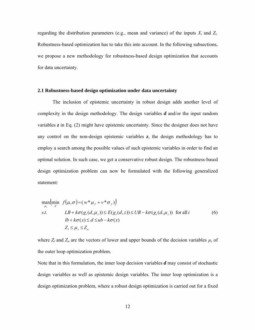
regarding the distribution parameters (e.g., mean and variance) of the inputs Xi and Zi.

Robustness-based optimization has to take this into account. In the following subsections,

we propose a new methodology for robustness-based design optimization that accounts

for data uncertainty.

2.1 Robustness-based design optimization under data uncertainty

The inclusion of epistemic uncertainty in robust design adds another level of

complexity in the design methodology. The design variables d and/or the input random

variables z in Eq. (2) might have epistemic uncertainty. Since the designer does not have

any control on the non-design epistemic variables z, the design methodology has to

employ a search among the possible values of such epistemic variables in order to find an

optimal solution. In such case, we get a conservative robust design. The robustness-based

design optimization problem can now be formulated with the following generalized

statement:

where Zl and Zu are the vectors of lower and upper bounds of the decision variables µz of

the outer loop optimization problem.

Note that in this formulation, the inner loop decision variables d may consist of stochastic

design variables as well as epistemic design variables. The inner loop optimization is a

design optimization problem, where a robust design optimization is carried out for a fixed

uzl

ziizi

ffd

ZZ

xkubdxklb

idgkUBzdgEdgkLBts

vwfz

)()(

)6( allfor )),(()),(()),((..

)**(,minmax

13

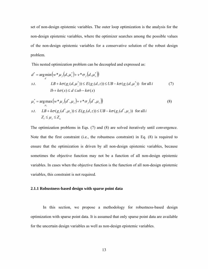
set of non-design epistemic variables. The outer loop optimization is the analysis for the

non-design epistemic variables, where the optimizer searches among the possible values

of the non-design epistemic variables for a conservative solution of the robust design

problem.

This nested optimization problem can be decoupled and expressed as:

)()(

)7( allfor )),(()),(()),((..

,*,*minarg

**

***

xkubdxklb

idgkUBzdgEdgkLBts

dvdwd

zz iii

zfzfd

uzl

ziizi

zfzfz

ZZ

idgkUBzdgEdgkLBts

dvdwz

allfor )),(()),(()),((..

)8(,*,*maxarg

**

***

The optimization problems in Eqs. (7) and (8) are solved iteratively until convergence.

Note that the first constraint (i.e., the robustness constraint) in Eq. (8) is required to

ensure that the optimization is driven by all non-design epistemic variables, because

sometimes the objective function may not be a function of all non-design epistemic

variables. In cases when the objective function is the function of all non-design epistemic

variables, this constraint is not required.

2.1.1 Robustness-based design with sparse point data

In this section, we propose a methodology for robustness-based design

optimization with sparse point data. It is assumed that only sparse point data are available

for the uncertain design variables as well as non-design epistemic variables.

14

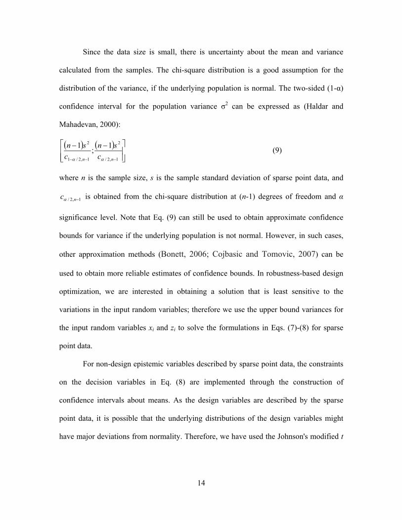
Since the data size is small, there is uncertainty about the mean and variance

calculated from the samples. The chi-square distribution is a good assumption for the

distribution of the variance, if the underlying population is normal. The two-sided (1-α)

confidence interval for the population variance σ2 can be expressed as (Haldar and

Mahadevan, 2000):

1,2/

2

1,2/1

2 1;

1

nn c

sn

c

sn

(9)

where n is the sample size, s is the sample standard deviation of sparse point data, and

1,2/ nc is obtained from the chi-square distribution at (n-1) degrees of freedom and α

significance level. Note that Eq. (9) can still be used to obtain approximate confidence

bounds for variance if the underlying population is not normal. However, in such cases,

other approximation methods (Bonett, 2006; Cojbasic and Tomovic, 2007) can be

used to obtain more reliable estimates of confidence bounds. In robustness-based design

optimization, we are interested in obtaining a solution that is least sensitive to the

variations in the input random variables; therefore we use the upper bound variances for

the input random variables xi and zi to solve the formulations in Eqs. (7)-(8) for sparse

point data.

For non-design epistemic variables described by sparse point data, the constraints

on the decision variables in Eq. (8) are implemented through the construction of

confidence intervals about means. As the design variables are described by the sparse

point data, it is possible that the underlying distributions of the design variables might

have major deviations from normality. Therefore, we have used the Johnson's modified t

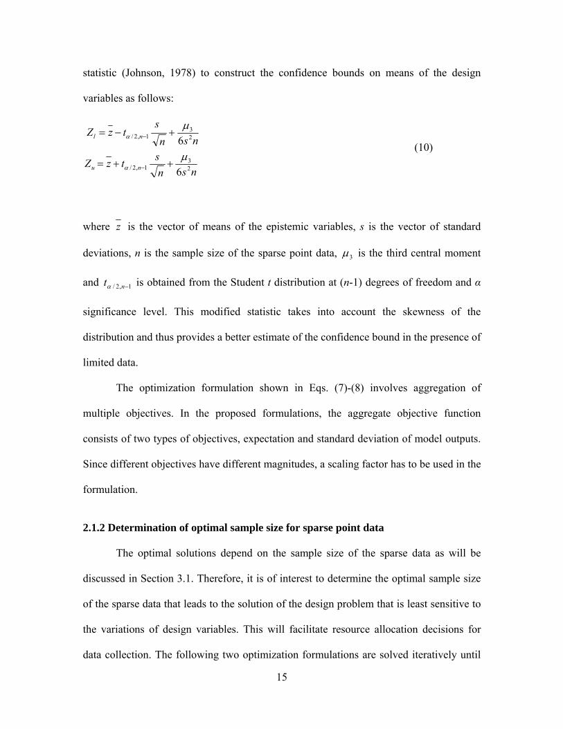
15

statistic (Johnson, 1978) to construct the confidence bounds on means of the design

variables as follows:

nsn

stzZ

nsn

stzZ

nu

nl

23

1,2/

23

1,2/

6

6

(10)

where z is the vector of means of the epistemic variables, s is the vector of standard

deviations, n is the sample size of the sparse point data, 3 is the third central moment

and 1,2/ nt is obtained from the Student t distribution at (n-1) degrees of freedom and α

significance level. This modified statistic takes into account the skewness of the

distribution and thus provides a better estimate of the confidence bound in the presence of

limited data.

The optimization formulation shown in Eqs. (7)-(8) involves aggregation of

multiple objectives. In the proposed formulations, the aggregate objective function

consists of two types of objectives, expectation and standard deviation of model outputs.

Since different objectives have different magnitudes, a scaling factor has to be used in the

formulation.

2.1.2 Determination of optimal sample size for sparse point data

The optimal solutions depend on the sample size of the sparse data as will be

discussed in Section 3.1. Therefore, it is of interest to determine the optimal sample size

of the sparse data that leads to the solution of the design problem that is least sensitive to

the variations of design variables. This will facilitate resource allocation decisions for

data collection. The following two optimization formulations are solved iteratively until

16

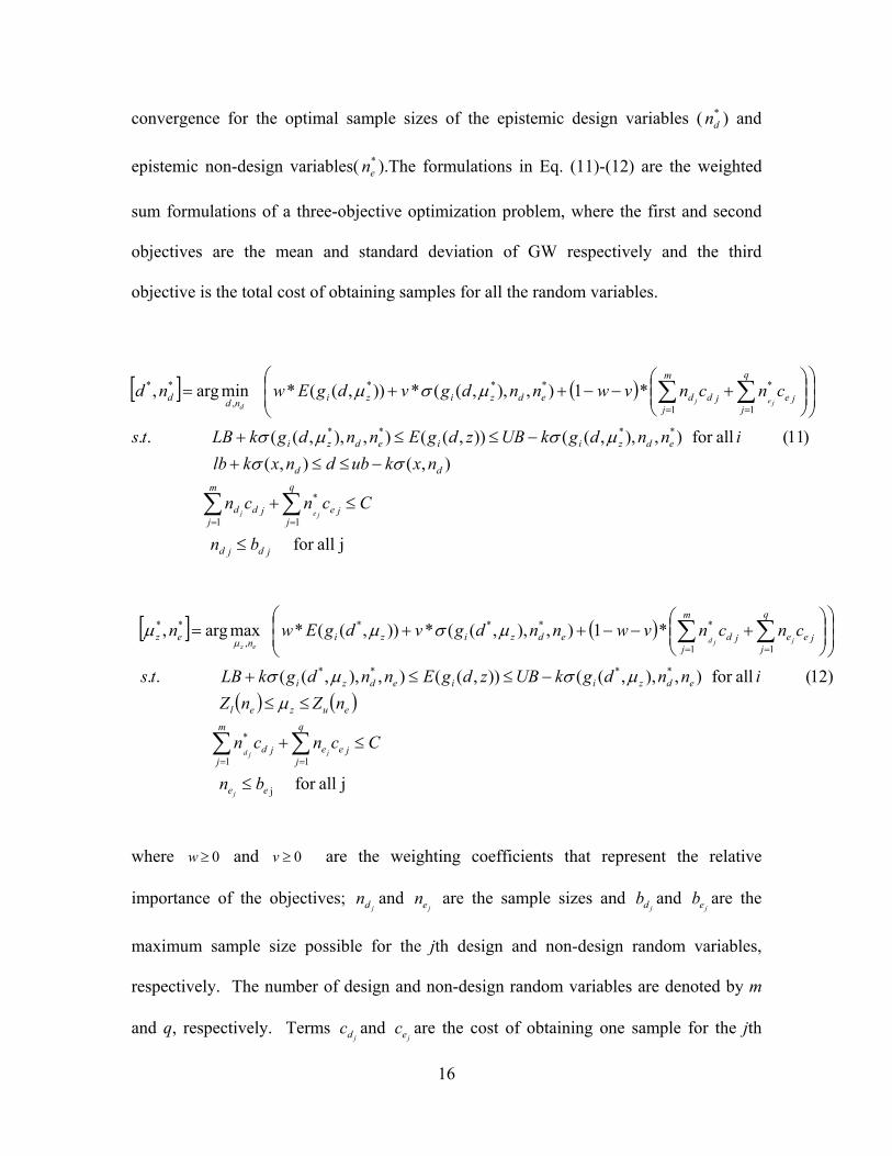
convergence for the optimal sample sizes of the epistemic design variables ( *dn ) and

epistemic non-design variables( *en ).The formulations in Eq. (11)-(12) are the weighted

sum formulations of a three-objective optimization problem, where the first and second

objectives are the mean and standard deviation of GW respectively and the third

objective is the total cost of obtaining samples for all the random variables.

where 0w and 0v are the weighting coefficients that represent the relative

importance of the objectives; jdn and

jen are the sample sizes and jdb and

jeb are the

maximum sample size possible for the jth design and non-design random variables,

respectively. The number of design and non-design random variables are denoted by m

and q, respectively. Terms jdc and

jec are the cost of obtaining one sample for the jth

j allfor

),(),(

)11( allfor ),),,(()),((),),,((..

*1),),,((*)),((*minarg,

1

*

1

****

1

*

1

***

,

**

jdjd

je

q

jjd

m

jd

dd

edziiedzi

je

q

jjd

m

jdedzizi

ndd

bn

Ccncn

nxkubdnxklb

inndgkUBzdgEnndgkLBts

cncnvwnndgvdgEwnd

jej

jejd

j allfor

)12( allfor ),),,(()),((),),,((..

*1),),,((*)),((*maxarg,

j

11

*

****

11

****

,

**

ee

je

q

jejd

m

j

euzel

edziiedzi

je

q

jejd

m

jedzizi

nez

bn

Ccncn

nZnZ

inndgkUBzdgEnndgkLBts

cncnvwnndgvdgEwn

j

jjd

jjdez

17

random design and non-design variables, respectively and C is the total cost allocated for

obtaining samples for all the random variables. Note that as in Eq. (8), the robustness

constraint in Eq. (12) is only required if the objective function is not a function of all non-

design epistemic variables. The optimization formulation presented above is a mixed-

integer nonlinear problem. A relaxed problem is solved in Section 3.

2.1.3 Robustness-based design with interval data

This section proposes a methodology for robustness-based design optimization

with interval data. In this case, the only information available for one or more input

random variables is in the form of single interval or multiple interval data. The following

discussion develops a methodology to solve the formulations in Eq. (7)-(8) for

uncertainty represented through interval data.

For interval data, the moments (e.g., mean and variance) are not a single value,

rather only bounds can be given (Zaman et al, 2009). We have proposed methods to

compute the bounds of moments for both single and multiple interval data in Zaman et al

(2009).The methods for computing bounds of the first two moments for interval data are

given later in this section. Once the bounds on the mean and variance of interval data are

estimated, we use the upper bounds of sample variance to solve the formulations of

robust design under uncertainty represented through single interval or multiple interval

data. Therefore, the resulting solution becomes least sensitive to the variations in the

uncertain variables.

18

For non-design epistemic variables described by interval data, the constraints on

the decision variables in Eqs. (8) and (12) are implemented through estimating the

bounds of the means by the methods as described later in this section.

The following discussions briefly summarize the methods to estimate the bounds

on the first two moments for single interval and multiple interval data, respectively.

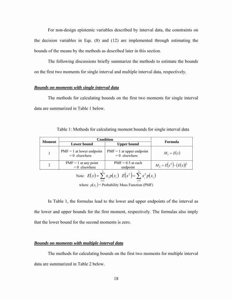
Bounds on moments with single interval data

The methods for calculating bounds on the first two moments for single interval

data are summarized in Table 1 below.

Table 1: Methods for calculating moment bounds for single interval data

Moment Condition

Formula Lower bound Upper bound

1 PMF = 1 at lower endpoint = 0 elsewhere

PMF = 1 at upper endpoint = 0 elsewhere

2 PMF = 1 at any point

= 0 elsewhere PMF = 0.5 at each

endpoint

Note:

where = Probability Mass Function (PMF)

In Table 1, the formulas lead to the lower and upper endpoints of the interval as

the lower and upper bounds for the first moment, respectively. The formulas also imply

that the lower bound for the second moments is zero.

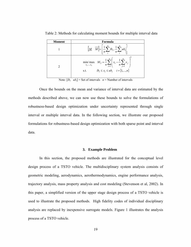
Bounds on moments with multiple interval data

The methods for calculating bounds on the first two moments for multiple interval

data are summarized in Table 2 below.

xEM 1

222 xExEM

ii

i xpxxE

2

1

ii

xpxxEi

2

1

22

ixp

19

Table 2: Methods for calculating moment bounds for multiple interval data

Moment Formula

1

n

i

n

iii ub

nlb

nMM

1,

1

2 niubxlb

xn

xn

M

iii

n

i

n

jji

xx n

,...,1s.t.

11maxmin/

2

1 12

,...,1

Note: [lbi ubi] = Set of intervals n = Number of intervals

Once the bounds on the mean and variance of interval data are estimated by the

methods described above, we can now use these bounds to solve the formulations of

robustness-based design optimization under uncertainty represented through single

interval or multiple interval data. In the following section, we illustrate our proposed

formulations for robustness-based design optimization with both sparse point and interval

data.

3. Example Problem

In this section, the proposed methods are illustrated for the conceptual level

design process of a TSTO vehicle. The multidisciplinary system analysis consists of

geometric modeling, aerodynamics, aerothermodynamics, engine performance analysis,

trajectory analysis, mass property analysis and cost modeling (Stevenson et al, 2002). In

this paper, a simplified version of the upper stage design process of a TSTO vehicle is

used to illustrate the proposed methods. High fidelity codes of individual disciplinary

analysis are replaced by inexpensive surrogate models. Figure 1 illustrates the analysis

process of a TSTO vehicle.

20

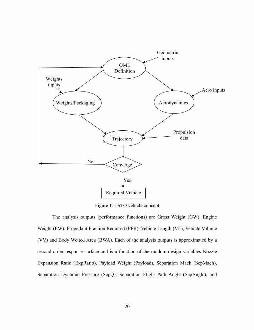
Figure 1: TSTO vehicle concept

The analysis outputs (performance functions) are Gross Weight (GW), Engine

Weight (EW), Propellant Fraction Required (PFR), Vehicle Length (VL), Vehicle Volume

(VV) and Body Wetted Area (BWA). Each of the analysis outputs is approximated by a

second-order response surface and is a function of the random design variables Nozzle

Expansion Ratio (ExpRatio), Payload Weight (Payload), Separation Mach (SepMach),

Separation Dynamic Pressure (SepQ), Separation Flight Path Angle (SepAngle), and

Yes

Required Vehicle

Weights inputs

Propulsion data

Converge No

Aero inputs

Geometric inputs

OML Definition

Aerodynamics Weights/Packaging

Trajectory

21

Body Fineness Ratio (Fineness). Each of the random variables is described by either

sparse point data or interval data.

The objective is to optimize an individual analysis output (e.g., Gross Weight)

while satisfying the constraints imposed by each of the design variables as well as all the

analysis outputs. We note here that we have assumed independence among the uncertain

input variables and thereby ignored the covariance terms in Eq. (5) to estimate the

variance of the performance function in each of the following examples. The numerical

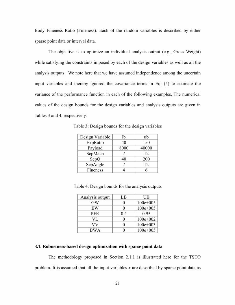
values of the design bounds for the design variables and analysis outputs are given in

Tables 3 and 4, respectively.

Table 3: Design bounds for the design variables

Design Variable lb ub ExpRatio 40 150 Payload 8000 40000

SepMach 7 12 SepQ 40 200

SepAngle 7 12 Fineness 4 6

Table 4: Design bounds for the analysis outputs

Analysis output LB UB GW 0 100e+005EW 0 100e+005PFR 0.4 0.95 VL 0 100e+002VV 0 100e+003

BWA 0 100e+005

3.1. Robustness-based design optimization with sparse point data

The methodology proposed in Section 2.1.1 is illustrated here for the TSTO

problem. It is assumed that all the input variables x are described by sparse point data as

22

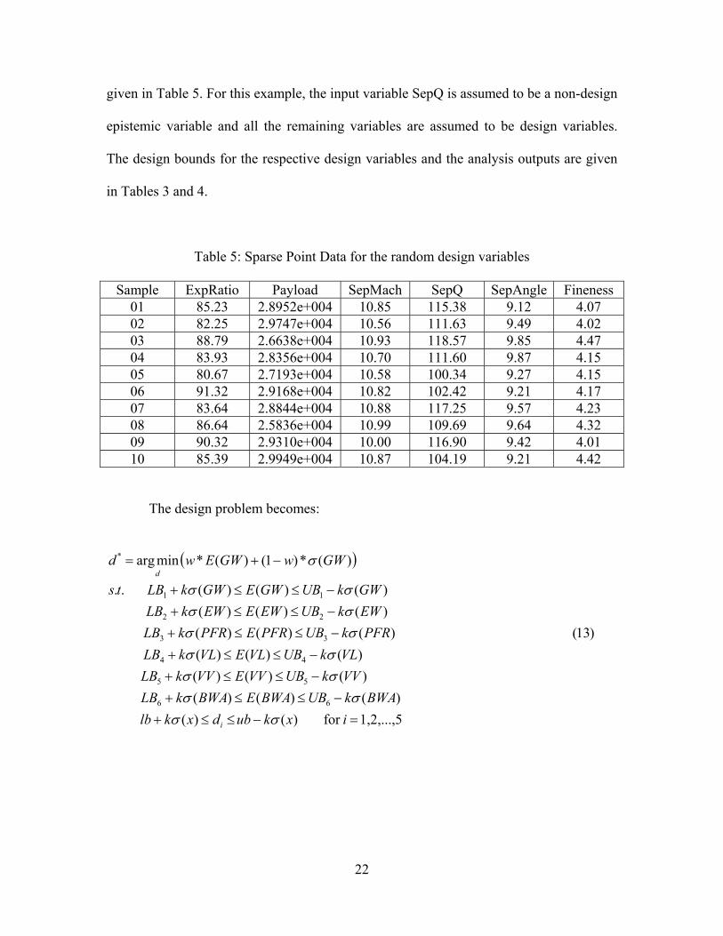
given in Table 5. For this example, the input variable SepQ is assumed to be a non-design

epistemic variable and all the remaining variables are assumed to be design variables.

The design bounds for the respective design variables and the analysis outputs are given

in Tables 3 and 4.

Table 5: Sparse Point Data for the random design variables

Sample ExpRatio Payload SepMach SepQ SepAngle Fineness 01 85.23 2.8952e+004 10.85 115.38 9.12 4.07 02 82.25 2.9747e+004 10.56 111.63 9.49 4.02 03 88.79 2.6638e+004 10.93 118.57 9.85 4.47 04 83.93 2.8356e+004 10.70 111.60 9.87 4.15 05 80.67 2.7193e+004 10.58 100.34 9.27 4.15 06 91.32 2.9168e+004 10.82 102.42 9.21 4.17 07 83.64 2.8844e+004 10.88 117.25 9.57 4.23 08 86.64 2.5836e+004 10.99 109.69 9.64 4.32 09 90.32 2.9310e+004 10.00 116.90 9.42 4.01 10 85.39 2.9949e+004 10.87 104.19 9.21 4.42

The design problem becomes:

1,2,...,5for )()(

)()()(

)()()(

)()()(

)13()()()(

)()()(

)()()(..

)(*)1()(*minarg

66

55

44

33

22

11

*

ixkubdxklb

BWAkUBBWAEBWAkLB

VVkUBVVEVVkLB

VLkUBVLEVLkLB

PFRkUBPFREPFRkLB

EWkUBEWEEWkLB

GWkUBGWEGWkLBts

GWwGWEwd

i

d

23

1for..

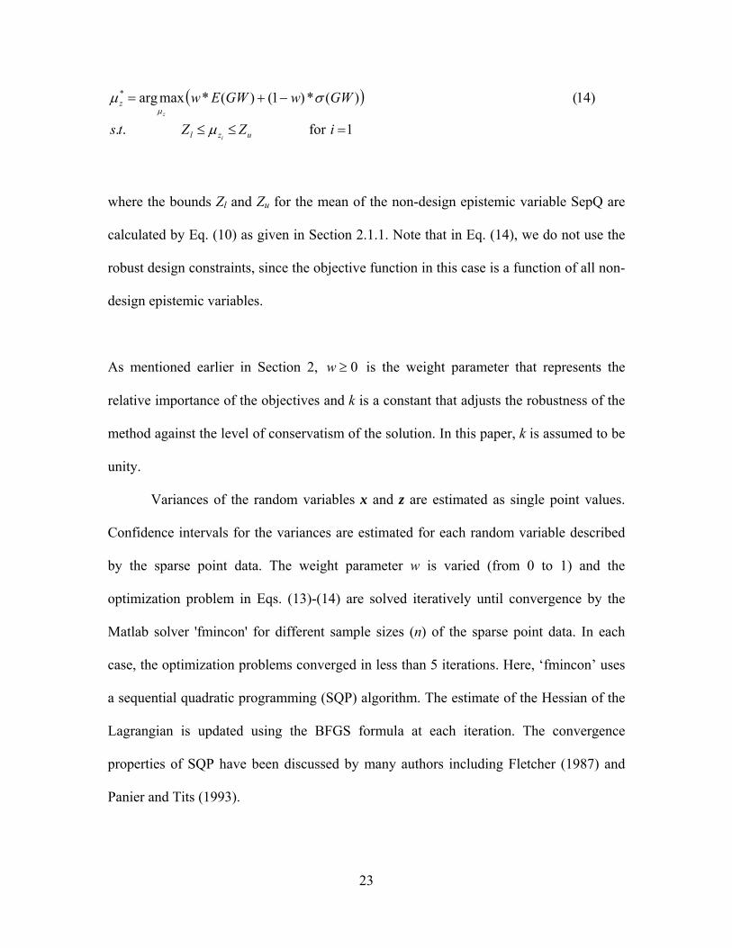
)14()(*)1()(*maxarg*

iZZts

GWwGWEw

uzl

z

i

z

where the bounds Zl and Zu for the mean of the non-design epistemic variable SepQ are

calculated by Eq. (10) as given in Section 2.1.1. Note that in Eq. (14), we do not use the

robust design constraints, since the objective function in this case is a function of all non-

design epistemic variables.

As mentioned earlier in Section 2, 0w is the weight parameter that represents the

relative importance of the objectives and k is a constant that adjusts the robustness of the

method against the level of conservatism of the solution. In this paper, k is assumed to be

unity.

Variances of the random variables x and z are estimated as single point values.

Confidence intervals for the variances are estimated for each random variable described

by the sparse point data. The weight parameter w is varied (from 0 to 1) and the

optimization problem in Eqs. (13)-(14) are solved iteratively until convergence by the

Matlab solver 'fmincon' for different sample sizes (n) of the sparse point data. In each

case, the optimization problems converged in less than 5 iterations. Here, ‘fmincon’ uses

a sequential quadratic programming (SQP) algorithm. The estimate of the Hessian of the

Lagrangian is updated using the BFGS formula at each iteration. The convergence

properties of SQP have been discussed by many authors including Fletcher (1987) and

Panier and Tits (1993).

24

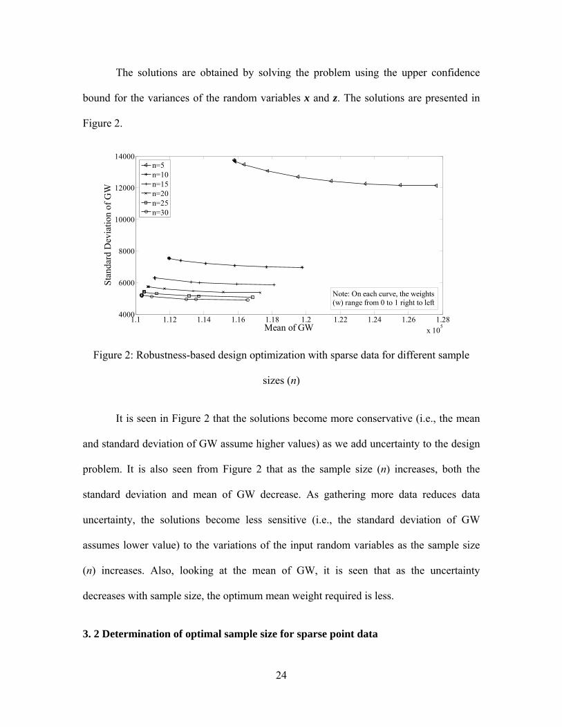
The solutions are obtained by solving the problem using the upper confidence

bound for the variances of the random variables x and z. The solutions are presented in

Figure 2.

Figure 2: Robustness-based design optimization with sparse data for different sample

sizes (n)

It is seen in Figure 2 that the solutions become more conservative (i.e., the mean

and standard deviation of GW assume higher values) as we add uncertainty to the design

problem. It is also seen from Figure 2 that as the sample size (n) increases, both the

standard deviation and mean of GW decrease. As gathering more data reduces data

uncertainty, the solutions become less sensitive (i.e., the standard deviation of GW

assumes lower value) to the variations of the input random variables as the sample size

(n) increases. Also, looking at the mean of GW, it is seen that as the uncertainty

decreases with sample size, the optimum mean weight required is less.

3. 2 Determination of optimal sample size for sparse point data

1.1 1.12 1.14 1.16 1.18 1.2 1.22 1.24 1.26 1.28

x 105

4000

6000

8000

10000

12000

14000

Mean of GW

Sta

ndar

d D

evia

tion

of G

W

n=5n=10n=15n=20n=25n=30

Note: On each curve, the weights(w) range from 0 to 1 right to left

25

The optimal sample size formulations are illustrated here for the TSTO design

problem. The formulations are relaxed by assuming that standard deviations of the data

do not change significantly as sample size changes. To make the problem simpler, we

first relax the integer requirement on the optimal sample size n and then round off the

solution for n to the nearest integer value. The input variable SepQ is assumed to be a

non-design epistemic variable and all the remaining variables are assumed to be design

variables. The design bounds for the respective design variables and the analysis outputs

remain the same as in Tables 3 and 4.

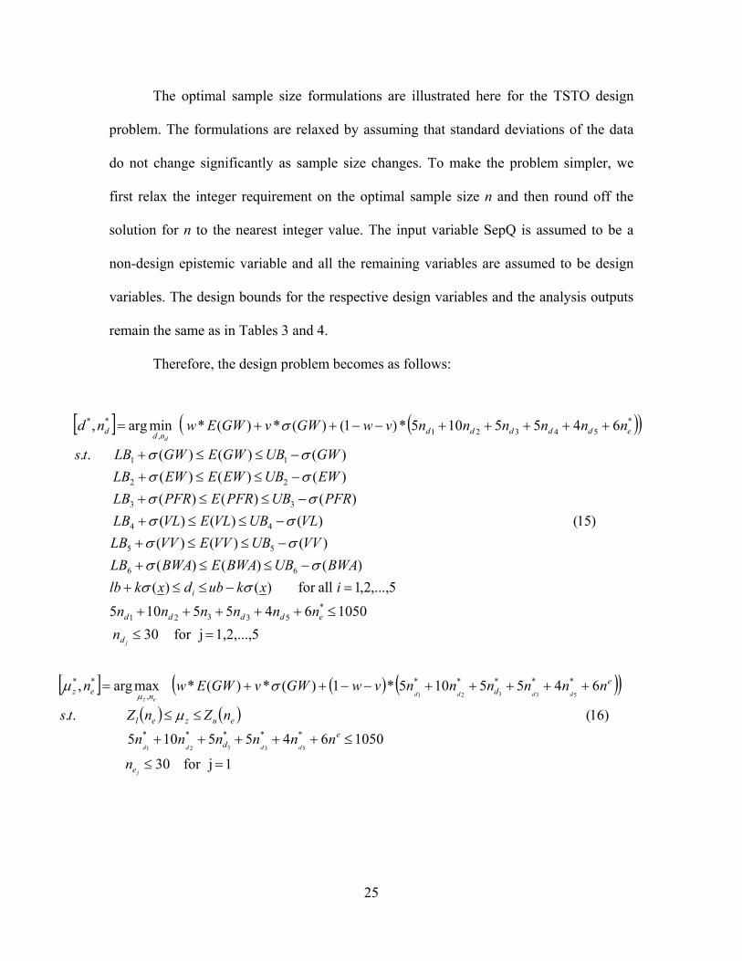
Therefore, the design problem becomes as follows:

1,2,...,5jfor 30

10506455105

5,...,2,1allfor )()(

)()()(

)()()(

)15()()()(

)()()(

)()()(

)()()(..

6455105*)1()(*)(*minarg,

*53321

66

55

44

33

22

11

*54321,

**

j

d

d

edddd

i

edddddnd

d

n

nnnnnn

ixkubdxklb

BWAUBBWAEBWALB

VVUBVVEVVLB

VLUBVLEVLLB

PFRUBPFREPFRLB

EWUBEWEEWLB

GWUBGWEGWLBts

nnnnnnvwGWvGWEwnd

1jfor 30

10506455105

)16(..

6455105*1)(*)(*maxarg,

*****

*****

,

**

53321

53321

j

dddd

ddddez

e

ed

euzel

ed

nez

n

nnnnnn

nZnZts

nnnnnnvwGWvGWEwn

26

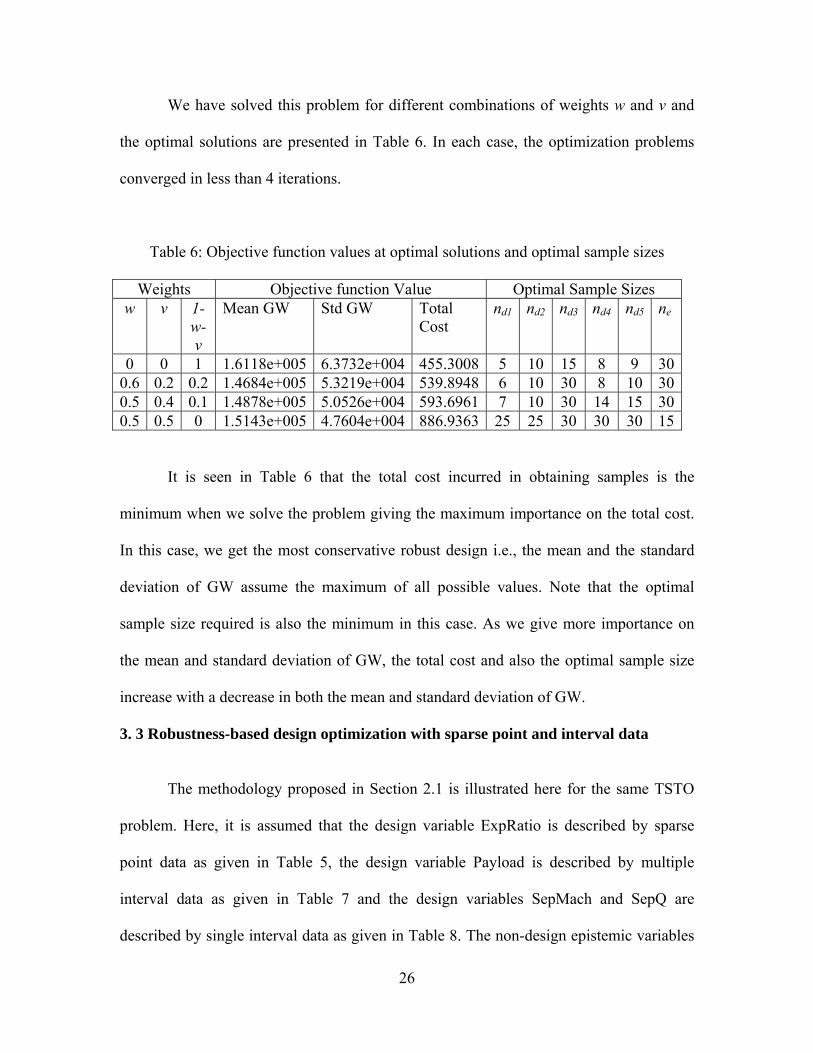
We have solved this problem for different combinations of weights w and v and

the optimal solutions are presented in Table 6. In each case, the optimization problems

converged in less than 4 iterations.

Table 6: Objective function values at optimal solutions and optimal sample sizes

Weights Objective function Value Optimal Sample Sizes w v 1-

w-v

Mean GW Std GW Total Cost

nd1 nd2 nd3 nd4 nd5 ne

0 0 1 1.6118e+005 6.3732e+004 455.3008 5 10 15 8 9 300.6 0.2 0.2 1.4684e+005 5.3219e+004 539.8948 6 10 30 8 10 300.5 0.4 0.1 1.4878e+005 5.0526e+004 593.6961 7 10 30 14 15 300.5 0.5 0 1.5143e+005 4.7604e+004 886.9363 25 25 30 30 30 15

It is seen in Table 6 that the total cost incurred in obtaining samples is the

minimum when we solve the problem giving the maximum importance on the total cost.

In this case, we get the most conservative robust design i.e., the mean and the standard

deviation of GW assume the maximum of all possible values. Note that the optimal

sample size required is also the minimum in this case. As we give more importance on

the mean and standard deviation of GW, the total cost and also the optimal sample size

increase with a decrease in both the mean and standard deviation of GW.

3. 3 Robustness-based design optimization with sparse point and interval data

The methodology proposed in Section 2.1 is illustrated here for the same TSTO

problem. Here, it is assumed that the design variable ExpRatio is described by sparse

point data as given in Table 5, the design variable Payload is described by multiple

interval data as given in Table 7 and the design variables SepMach and SepQ are

described by single interval data as given in Table 8. The non-design epistemic variables

27

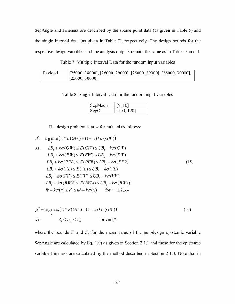
SepAngle and Fineness are described by the sparse point data (as given in Table 5) and

the single interval data (as given in Table 7), respectively. The design bounds for the

respective design variables and the analysis outputs remain the same as in Tables 3 and 4.

Table 7: Multiple Interval Data for the random input variables

Payload [25000, 28000], [26000, 29000], [25000, 29000], [26000, 30000], [25000, 30000]

Table 8: Single Interval Data for the random input variables

SepMach [9, 10] SepQ [100, 120]

The design problem is now formulated as follows:

1,2,3,4for )()(

)()()(

)()()(

)()()(

)15()()()(

)()()(

)()()(..

)(*)1()(*minarg

66

55

44

33

22

11

*

ixkubdxklb

BWAkUBBWAEBWAkLB

VVkUBVVEVVkLB

VLkUBVLEVLkLB

PFRkUBPFREPFRkLB

EWkUBEWEEWkLB

GWkUBGWEGWkLBts

GWwGWEwd

i

d

2,1for..

)16()(*)1()(*maxarg*

iZZts

GWwGWEw

uzl

z

i

z

where the bounds Zl and Zu for the mean value of the non-design epistemic variable

SepAngle are calculated by Eq. (10) as given in Section 2.1.1 and those for the epistemic

variable Fineness are calculated by the method described in Section 2.1.3. Note that in

28

Eq. (16), we do not use the robust design constraints, since the objective function in this

case is a function of all non-design epistemic variables.

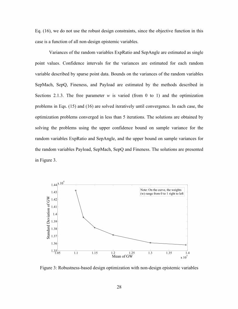
Variances of the random variables ExpRatio and SepAngle are estimated as single

point values. Confidence intervals for the variances are estimated for each random

variable described by sparse point data. Bounds on the variances of the random variables

SepMach, SepQ, Fineness, and Payload are estimated by the methods described in

Sections 2.1.3. The free parameter w is varied (from 0 to 1) and the optimization

problems in Eqs. (15) and (16) are solved iteratively until convergence. In each case, the

optimization problems converged in less than 5 iterations. The solutions are obtained by

solving the problems using the upper confidence bound on sample variance for the

random variables ExpRatio and SepAngle, and the upper bound on sample variances for

the random variables Payload, SepMach, SepQ and Fineness. The solutions are presented

in Figure 3.

Figure 3: Robustness-based design optimization with non-design epistemic variables

1.05 1.1 1.15 1.2 1.25 1.3 1.35 1.4

x 105

1.35

1.36

1.37

1.38

1.39

1.4

1.41

1.42

1.43

1.44 x 104

Mean of GW

Stan

dard

Dev

iatio

n of

GW

Note: On the curve, the weights(w) range from 0 to 1 right to left

29

Figure 3 shows the solutions of the conservative robust design in presence of

uncontrollable epistemic uncertainty described through mixed data i.e., both sparse point

data and interval data, which is seen frequently in many engineering applications.

4. Summary and Conclusion

This paper proposed several formulations for robustness-based design

optimization under data uncertainty. Two types of data uncertainty – sparse point data

and interval data – are considered. The proposed formulations are illustrated for the upper

stage design problem of a TSTO space vehicle. A decoupled approach is proposed in this

paper to un-nest the robustness-based design from the analysis of non-design epistemic

variables to achieve computational efficiency. As gathering more data reduces

uncertainty but increases cost, the effect of sample size on the optimality and the

robustness of the solution is also studied. This is demonstrated by numerical examples,

which suggest that as the uncertainty decreases with sample size, the resulting solutions

become more robust. We have also proposed a formulation to determine the optimal

sample size for sparse point data that leads to the solution of the design problem that is

least sensitive (i.e., robust) to the variations of design variables. In this paper, we have

used the weighted sum approach for the aggregation of multiple objectives and to

examine the trade-offs among multiple objectives. Other multi-objective optimization

techniques can also be explored within the proposed formulations.

The major advantage of the proposed methodology is that unlike existing

methods, it does not use separate representations for aleatory and epistemic uncertainties

and does not require nested analysis. Both types of uncertainty are treated in a unified

30

manner using a probabilistic format, thus reducing the computational effort and

simplifying the optimization problem. The results regarding robustness of the design

versus data size are valuable to the decision maker. The design optimization procedure

also optimizes the sample size, thus facilitating resource allocation for data collection

efforts. Due to the use of a probabilistic format to represent all the uncertain variables,

the proposed robustness-based design optimization methodology facilitates the

implementation of multidisciplinary robustness-based design optimization, which is a

challenging problem in presence of epistemic uncertainty.

Acknowledgement

This study was supported by funds from NASA Langley Research Center under Cooperative Agreement No. NNX08AF56A1 (Technical Monitor: Mr. Lawrence Green). The support is gratefully acknowledged. References: [1] Agarwal, H, Mozumder, C K, Renaud, J E, and Watson, L T, An inverse-measure-based unilevel architecture for reliability-based design optimization, Struct Multidisc Optim (2007) 33: 217–227. [2] Bichon, B J, McFarland, J M and Mahadevan, S, Using Bayesian Inference and Efficient Global Reliability Analysis to Explore Distribution Uncertainty, 49th AIAA/ASME/ASCE/AHS/ASC Structures, Structural Dynamics, and Materials Conference, 7 - 10 April 2008, Schaumburg, IL. [3] Bras, B. A., and Mistree, F., 1993, Robust Design using Compromise Decision Support Problems, Engineering Optimization, Vol. 21, pp. 213-239.

[4] Bras, B. A. and Mistree, F., 1995, A Compromise Decision Support Problem for Robust and Axiomatic Design, ASME Journal of Mechanical Design, Vol. 117, No. 1, pp. 10-19.

[5] Bonett, D G., Approximate confidence interval for standard deviation of nonnormal distributions, Computational Statistics & Data Analysis 50 (2006) 775 – 782.

31

[6] Cagan, J., Williams, B. C., 1993, First-Order Necessary Conditions for Robust Optimality, in ASME Advances in Design Automation, Albuquerque, NM, ASME DE-Vol. 65-1.

[7] Chen, W., Allen, J. K., Mistree, F. and Tsui, K.-L., 1996, A Procedure for Robust Design: Minimizing Variations Caused by Noise Factors and Control Factors, ASME Journal of Mechanical Design, Vol. 118, pp.478-485.

[8] Chen W, Wiecek MM, Zhang J., Quality utility—a compromise programming approach to robust design, Journal of Mechanical Design (ASME) 1999; 121:179–187.

[9] Chen, W., Sahai, A., Messac, A., Sundararaj, G.J., Exploration of the effectiveness of physical programming in robust design, J. Mech. Des. 122, 155–163, 2000.

[10] Cheng, H and Sandu, A, Efficient uncertainty quantification with the polynomial chaos method for stiff systems, Mathematics and Computers in Simulation 79 (2009) 3278–3295.

[11] Chiralaksanakul, A., and Mahadevan, S., First-Order Approximation Methods in Reliability-Based Design Optimization, J. Mech. Des.,Volume 127, Issue 5, 2005. [12] Cojbasic, V., Tomovic, A., Nonparametric confidence intervals for population variance of one sample and the difference of variances of two samples, Computational Statistics & Data Analysis 51 (2007) 5562 – 5578. [13] Dai, Z, and Mourelatos, Z P, Incorporating Epistemic Uncertainty in Robust Design, Proceedings of DETC, 2003 ASME Design Engineering Technical Conferences September 2-6, 2003, Chicago, Illinois, USA. [14] Doltsinis, I, and Kang, Z, Robust design of structures using optimization methods, Comput, Methods Appl. Mech. Engrg. 193 (2004) 2221–2237. [15] Du, X., and Chen, W., Towards a better understanding of Modeling Feasibility Robustness in Engineering, ASME J. Meach. Des., 2000, 122(4). [16] Du. X, Sudjianto, A., Chen. W., An Integrated Framework for Optimization Under Uncertainty Using Inverse Reliability Strategy, ASME, 2004. [17] Du, X, and Beiqing Huang, B, Reliability-based design optimization with equality constraints, Int. J. Numer. Meth. Engng 2007; 72:1314–1331. [18] Fletcher, R, Practical Methods of Optimization, 2nd ed. John Wiley, New York, 1987.

32

[19] Ghanem, R., and Spanos, P., Stochastic Finite Elements: A Spectral Approach, Springer-Verlag, New York, 1991. [20] Haldar A., Mahadevan S., Probability, Reliability and Statistical Methods in Engineering Design, John Wiley & Sons, Inc., 2000. [21] Hong, HP, An efficient point estimate method for probabilistic analysis, Reliability Engineering and System Safety 59 (1998) 261-267.

[22] Huang, B., and Du, X, Analytical robustness assessment for robust design, Struct Multidisc Optim (2007) 34:123–137. [23] Johnson, N J., Modified t Tests and Confidence Intervals for Assymmetrical Populations, Journal of the American Statistical Association, Vol. 73, No. 363, Sep., 1978, pp. 536-544. [24] Lee, K-H, and Park, G-J, Robust optimization considering tolerances of design variables, Computers and Structures 79 (2001) 77-86. [25] Lee. I., Choi. K. K., Du. L., Gorsich. D., Dimension reduction method for reliability-based robust design optimization, Computers and Structures, 2008. [26] Marler, R T, and Arora, J S, Survey of multi-objective optimization methods for engineering, Struct Multidisc Optim 26, 369–395 (2004).

[27] Mavrotas, G, Effective implementation of the e-constraint method in Multi Objective Mathematical Programming problems, Applied Mathematics and Computation 213 (2009) 455–465. [28] Messac, A., Physical Programming Effective Optimization for Computational Design, AIAA Journal, Vol. 34, No. 1, 1996, pp. 149–158.

[29] Messac, A., Melachrinoudis, E., and Sukam, C. P., Mathematical and Pragmatic Perspectives of Physical Programming, AIAA Journal, Vol. 39, No. 5, 2001, pp. 885- 893. [30] Messac, A, and Ismail-Yahaya, A, Multiobjective robust design using physical programming, Struct Multidisc Optim 23, 357–371, 2002.

[31] Oberkampf WL, Helton JC, Joslyn CA, Wojtkiewicz SF, Ferson S, Challenge Problems: uncertainty in system response given uncertain parameters, Reliability Engineering and System Safety, 85 (2004) 11-19. [32] Panier, E R, and Tits, A L, On combining feasibility, descent and superlinear convergence in inequality constrained optimization, Mathematical Programming, 59:261–276, 1993.

33

[33] Park, G-J, Lee, T-H, Lee, KH, and Hwang, K-H, Robust Design: An Overview, AIAA JOURNAL, Vol. 44, No. 1, January 2006. [34] Parkinson, A., Sorensen, C., and Pourhassan, N., 1993, A General Approach for Robust Optimal Design, Transactions of the ASME, Vol. 115, pp.74-80. [35] Ramu, P., Qu, X., Youn, B.D., Haftka, R.T. and Choi, K.K. (2006) Inverse reliability measures and reliability-based design optimisation, Int. J. Reliability and Safety, Vol. 1, Nos. 1/2, pp.187–205.

[36] Robert, C. P. and Casella, G., Monte Carlo Statistical Methods. 2nd ed. Springer-Verlag, New York, 2004. [37] Rosenblueth E (1975), Point estimates for probability moment, Proc Natl Acad Sci U S A 72(10):3812–3814.

[38] Sim M., Robust Optimization, PhD dissertation submitted to the Sloan School of Management, Massachusetts Institute of Technology, June 2004.

[39] Stevenson M D, Hartong A R, Zweber J V, Bhungalia A A, Grandhi R V, Collaborative Design Environment for Space Launch Vehicle Design and Optimization, Paper presented at the RTO AVT Symposium on "Reduction of Military Vehicle Acquisition Time and Cost through Advanced Modeling and Virtual Simulation", held in Paris, France, April 2002. [40] Sundaresan, S., Ishii, K., and Houser, D. R., A Robust Optimization Procedure with Variations on Design Variables and Constraints, Engineering Optimization, Vol. 24, No. 2, 1995, pp. 101–117. [41] Taguchi, G., 1993, Taguchi on Robust Technology Development: Bringing Quality Engineering Upstream, ASME Press, New York. [42] Wei D L, Cui, Z S, and Chen, J, Robust optimization based on a polynomial expansion of chaos constructed with integration point rules, J. Mechanical Engineering Science, Vol. 223 Part C, 2009. [43] Youn, B D, Choi, K K, and Du, L, Integration of Possibility-Based Optimization and Robust Design for Epistemic Uncertainty, ASME Journal of Mechanical Design, Vol. 129, AUGUST 2007. [44] Yu, J-C and Ishii, K., 1998, Design for Robustness Based on Manufacturing Variation Patterns, Transactions of the ASME, Vol.120, pp. 196-202. [45] Zaman, K, Rangavajhala, S, McDonald, PM., and Mahadevan, S, 2009, A probabilistic approach for representation of interval uncertainty, Reliability Engineering and System Safety. (under review)

34

[46] Zeleny, M. 1973, Compromise programming, in: Multiple Criteria Decision Making, eds: J. L. Cochrane and M. Zeleny, University of South Carolina Press, Columbia, SC, pp. 262-301. [47] Zhang, W H, A compromise programming method using multibounds formulation and dual approach for multicriteria structural optimization, Int. J. Numer. Meth. Engng 2003; 58:661–678.

[48] Zhao, Y-G, Ono, T (2000), New point estimates for probability moments,, J Eng Mech 126(4):433–436.

[49] Zhao Y-G, Ang AH-S (2003), System reliability assessment by method of Moments, J Struct Eng 129(10):1341–1349.

[50] Zou, T, and Mahadevan, S, Versatile Formulation for Multiobjective Reliability-Based Design Optimization, J. Mech. Des. 128, 1217 (2006).