Rodrigues, D. J., Champneys, A. R., Friswell, M. I., & Wilson, R. E. (2010).Experimental investigation of a single-plane automatic balancing mechanismfor a rigid rotor.

Early version, also known as pre-print

Link to publication record in Explore Bristol ResearchPDF-document

University of Bristol - Explore Bristol ResearchGeneral rights

This document is made available in accordance with publisher policies. Please cite only the publishedversion using the reference above. Full terms of use are available:http://www.bristol.ac.uk/pure/about/ebr-terms

Experimental investigation of a single-plane automatic balancing

mechanism for a rigid rotor

D.J. Rodriguesa, A.R. Champneysa,∗, M.I. Friswellb and R.E. Wilsona

aDepartment of Engineering Mathematics, University of Bristol, Bristol, BS8 1TR, UKbSchool of Engineering, Swansea University, Swansea, SA2 8PP, UK

Abstract

We present an experimental investigation of a single-plane automatic balancer that is fitted to a rigid rotor.

Two balls, which are free to travel around a circular race, are used to compensate for the mass imbalance in

the plane of the device. The experimental rig possesses both cylindrical and conical rigid body modes and the

performance of the automatic balancer is assessed for a variety of different levels of imbalance. A non-planar

mathematical model that also includes the observed effect of support anisotropy is developed and numerical

simulations are compared with the experimental findings. In the highly supercritical frequency range the balls

act to balance the rotor and a good quantitative match is found between the model and the experimental data.

However, during the rigid body resonances the dynamics of the ball balancer is highly nonlinear and for this

speed range the agreement between theory and experiment is mainly qualitative. Nevertheless, the model is able

to successfully reproduce many of the solution types that are found experimentally.

1 Introduction

An automatic ball balancer (ABB) is a device which reduces vibrations in rotating machinery by compensating

for the mass imbalance of the rotor. The mechanism consists of a series of balls that are free to travel around

a race which is set at a fixed distance from the shaft. During balanced operation the balls find positions such

that the principal axis of inertia is repositioned onto the rotational axis. Because the imbalance does not need to

be determined beforehand, automatic balancers are ideally suited to applications where the amount of imbalance

varies with the operating conditions. For example, automatic balancers are currently used in optical disk drives,

machine tools and washing machines [14, 16, 1]. However, ABBs have not been more widely adopted, not least

because the mechanism is inherently nonlinear and displays extreme sensitivity to both rotation speed and initial

conditions. Therefore, whilst an ABB can successfully eliminate the imbalance for some supercritical speeds, it

can also make the vibration levels significantly worse during the rotor run-up. Nevertheless, recent advances in

the modelling of ABBs have led to improved predictions of their regions of stability [13, 17]. This paper aims to

validate those predictions.

The first study of an ABB was carried out by Thearle in 1932 [24], and the existence of a stable balanced steady

state at rotation speeds above the first critical frequency was demonstrated. More recently, the equations of motion

for a planar Jeffcott rotor with an ABB have been derived using Lagrange’s method [15, 7, 13]. In particular, Green

et al. [13] presented the first nonlinear bifurcation analysis of an ABB and the dynamics of the oscillating ball

states were explored. However, ABB models which are based on a Jeffcott rotor do not include any tilting motions

and so they are unable to explain phenomena that are related to principal axis misalignment. These out-of-plane

motions are considered in the theoretical studies of Chung and Jang [6], Chao et al. [3] and Sperling et al. [22],

however only linear stability analyses were provided.

Rodrigues et al. [17] investigated a two-plane ABB device that can compensate for both mass eccentricity and

principal axis misalignment. Rotating coordinates were used to derive an autonomous set of governing equations

and numerical continuation techniques were employed to compute the stability boundaries of the fully nonlinear

system in various parameter planes. Moreover, regions of bistability were found in which the balanced state coex-

ists with a desynchronized state that has the balls rotating at a different angular frequency to the rotor. Subsequent

theoretical studies by the same authors also considered the effect of unequal ball masses and support anisotropy

∗Corresponding author. E-mail: A.R.Champneys@bristol.ac.uk

1

[19, 18]. There it is shown that, provided the imbalance is small, the balanced state is robust to the considered

asymmetries.

Finally, contemporary experimental autobalancing research has primarily focused on systems that have been tai-

lored towards use in specific applications. For example, the effects of rolling friction between the race and the

balancing balls were observed in optical disk drive systems by Chao et al. [4], van de Wouw et al. [25] and Yang

et al. [27]. An experimental study into the influence of non-planar motions on the performance of the ABB was

also carried out by Chao et al. [5]. There, an optical disk drive equipped with a single-plane balancer was con-

sidered, and the vibration level of the rotor was measured as it passed through multiple resonances. In addition,

an investigation of a multi-ball system with a partitioned race was performed by Green et al. [12]. In that study

the motion of the balls was observed with the aid of a strobe light, however, large vibration amplitudes at the first

critical speed prevented measurements of the ABB dynamics beyond the first resonance.

Although these results are promising, the body of experimental evidence for the effective operation of an ABB

device remains scarce. In particular, data for the performance of an ABB in the highly supercritical frequency

range is still unavailable. In light of the absence of this empirical data, we have set out to design a lightweight,

low bearing support stiffness, table top rig. The set-up has been specifically designed to possess both cylindrical

and conical rigid body modes, and also, to allow the performance of the ball balancer to be safely observed up to

sufficiently high rotational frequencies. After the rig had been built, non-circular mode shapes were found to exist

and this indicated the presence of support anisotropy. Therefore, the mathematical model has also been extended

to include this effect.

The rest of this paper is organised as follows. In Section 2 we describe the overall experimental set-up and the

design of the automatic balancer is also discussed. The mathematical model is introduced in Section 3 and the

rotor parameters are estimated in Section 4. In Section 5 the response of the rotor in the absence of the balancing

balls is investigated, and these measurements are used to estimate the values of the support parameters. Next, in

Section 6 we present results of ABB frequency responses for a range of different imbalances. In Section 7 we

compare these experimental results with numerical simulations that are generated from the mathematical model.

Finally, in Section 8 we draw conclusions and discuss possible directions for future work.

ABB disk

Spring

Accelerometer

Bearing

Housing

Rubber band

Motor

Rigid coupling

Shaft

Support post

Figure 1: Photograph of the experimental rig.

2 Experimental set-up

A photograph of the experimental test rig is shown in Figure 1. The rig comprises of an ABB disk that is posi-

tioned midway along a horizontal silver steel shaft of 10mm diameter. This shaft is mounted at each end onto

nominally identical single-row ball bearings, which are fitted into housings and attached to the supports through

a set of springs. The support structure consists of four posts that are reinforced with lateral beams and fixed to

a wooden base board. Next, a motor that is suspended by rubber bands drives the shaft via a rigid coupling and

2

the speed of this motor is controlled through a dSpace DS1104 digital signal processing board [8]. Finally, the

lateral vibrations are measured with accelerometers that are attached to the bearing housings and the resulting

accelerations are converted into displacements with a simple Matlab routine.

Before we move onto a description of the ABB disk, we shall first explain some of the design choices that led to

this particular realisation of the experimental set-up. The requirement that the rotor should be capable of safely

operating at highly supercritical rotation speeds made it necessary that the rig should be both lightweight and

also have relatively low critical vibration frequencies. Therefore, we envisaged a rotor with a mass of around

1-2 kg and with critical frequencies somewhere in the 1000-3000 rpm range. By using the lower bounds of these

values in the expression for the first critical frequency Ω1 =√

k11/M , we can gain a rough initial estimate ofk11 ≈ 10,000Nm-1 for the desired lateral stiffness. This value is more than an order of magnitude less than

the corresponding stiffness coefficient of k = 3.436×105 Nm-1 for the system studied by Green et al. [12] in

which the bearing housings were bolted to an external frame. In light of this observation, our housings are not

rigidly fixed to ground but are instead supported by springs that give an appropriate stiffness. As a consequence,

the stiffness coefficient of our system will be more comparable to that of the optical disk drive set-ups studied in

[4, 25, 27].

Having established this ‘soft’ bearing support structure, the connection between the motor and shaft was required

to be as rigid as possible in order that we could avoid any undesirable vibrational modes that a flexible coupling

may have induced. With a rigid connection, the motor becomes an integral part of the rotor and therefore it must

also be lightweight. The motor that we have chosen for our rig is an ebm-papst ‘Variodrive’ VD-3-35.06 [9]; this

model is a three phase brushless design that has a mass of 120 g and a nominal top speed of 6200 rpm. The motor

is then suspended from rubber bands so that the lateral load on its spindle is reduced. The bands also allow the

generated torque to react against the frame so that the motor can drive the rotor.

In order to determine the system’s response, the vibrations at the bearing housings are measured with accelerom-

eters. An alternative would be to use a laser Doppler vibrometer, which would have the advantage of being

able to measure the vibration level directly at the ABB disk. However, as the rig operates in the rigid regime,

the vibration level at the disk can be inferred from those at the housings and the accelerometers are suitable for

this purpose. Finally, in order to allow the efficient production of high resolution frequency response curves, a

dSpace ControlDesk system was used to automate the experimental runs and data acquisition procedures.

Aluminium hub

Steel ball race

Screw

Rubber seal

Adjustable mass

Steel balls

Reference sticker

Figure 2: Photograph of the automatic balancer. Note, in this picture the balls are larger than those used in the

actual experiments cf. Figure 9.

The automatic balancer, which is shown in Figure 2, consists of an aluminium hub into which a hardened steel

ball race of 50mm outer radius has been fitted. Steel balls of 4.76mm diameter and 0.44 g mass are used as the

balancing masses. The balls can be viewed through a perspex cover that is attached to the balancer with a circular

array of screws. A light coating of oil, which provides damping for the motion of the balls, is applied to the race

and a rubber seal is used to prevent any oil from escaping. The balance of the disk can be adjusted, either by

adding washers to the screws, or by changing the angular position of adjustable outer masses that can be rotated

around a groove in the hub and fixed in place with grub screws.

At this point, let us highlight some considerations relating to the design of the ABB disk. The steel ball race

comes from the outer part of a single row, deep groove, SKF 16013 ‘explorer’ bearing. According to the company

literature [21], these bearings are made from a high grade steel that is cleaner and more homogeneous than that

3

which is used in their standard bearings. Also, the steel has been hardened through a heat treatment procedure and

the finish on the contact surface has also been improved. It is hoped that these features reduce the rolling friction

between the balls and the race and thereby improve the performance of the ABB [4, 25, 27]. In addition, the deep

groove in the race prevents the balls from rattling between the hub and the perspex cover, as during operation a

centrifugal force acts on the balls so that they are confined to lie in the deepest part of the channel.

3 Mathematical model

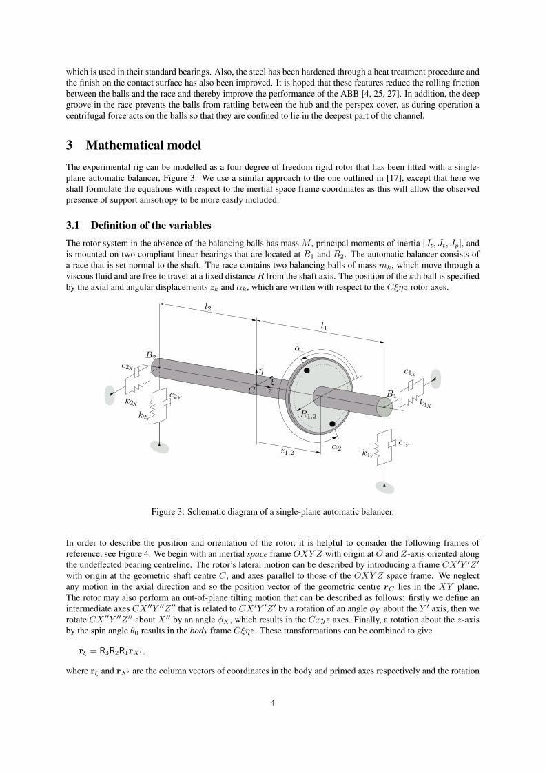
The experimental rig can be modelled as a four degree of freedom rigid rotor that has been fitted with a single-

plane automatic balancer, Figure 3. We use a similar approach to the one outlined in [17], except that here we

shall formulate the equations with respect to the inertial space frame coordinates as this will allow the observed

presence of support anisotropy to be more easily included.

3.1 Definition of the variables

The rotor system in the absence of the balancing balls has massM , principal moments of inertia [Jt, Jt, Jp], andis mounted on two compliant linear bearings that are located at B1 and B2. The automatic balancer consists of

a race that is set normal to the shaft. The race contains two balancing balls of mass mk, which move through a

viscous fluid and are free to travel at a fixed distanceR from the shaft axis. The position of the kth ball is specifiedby the axial and angular displacements zk and αk, which are written with respect to the Cξηz rotor axes.

l2

l1

z1,2

α1

α2

R1,2

Cξ

η

z

k1Y

k2Y

c1Y

c2Y

k1X

k2X

c1X

c2X

B1

B2

Figure 3: Schematic diagram of a single-plane automatic balancer.

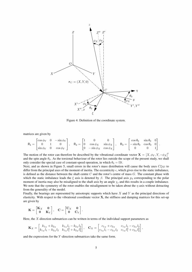
In order to describe the position and orientation of the rotor, it is helpful to consider the following frames of

reference, see Figure 4. We begin with an inertial space frame OXY Z with origin at O and Z-axis oriented alongthe undeflected bearing centreline. The rotor’s lateral motion can be described by introducing a frame CX ′Y ′Z ′

with origin at the geometric shaft centre C, and axes parallel to those of the OXY Z space frame. We neglectany motion in the axial direction and so the position vector of the geometric centre rC lies in the XY plane.The rotor may also perform an out-of-plane tilting motion that can be described as follows: firstly we define an

intermediate axes CX ′′Y ′′Z ′′ that is related to CX ′Y ′Z ′ by a rotation of an angle φY about the Y ′ axis, then we

rotate CX ′′Y ′′Z ′′ about X ′′ by an angle φX , which results in the Cxyz axes. Finally, a rotation about the z-axisby the spin angle θ0 results in the body frame Cξηz. These transformations can be combined to give

rξ = R3R2R1rX′ ,

where rξ and rX′ are the column vectors of coordinates in the body and primed axes respectively and the rotation

4

X Y

Z

ξ

y

η

O

X ′

Y ′, Y ′′

Z ′

X ′′, x

Z ′′

z

θ0

θ0

φX

φXφY

φY

C

rC = (X,Y, 0)

Figure 4: Definition of the coordinate system.

matrices are given by

R1 =

cos φY 0 − sin φY

0 1 0sin φY 0 cos φY

, R2 =

1 0 00 cos φX sin φX

0 − sin φX cos φX

, R3 =

cos θ0 sin θ0 0− sin θ0 cos θ0 0

0 0 1

.

The motion of the rotor can therefore be described by the vibrational coordinate vector X = [X,φY , Y,−φX ]T

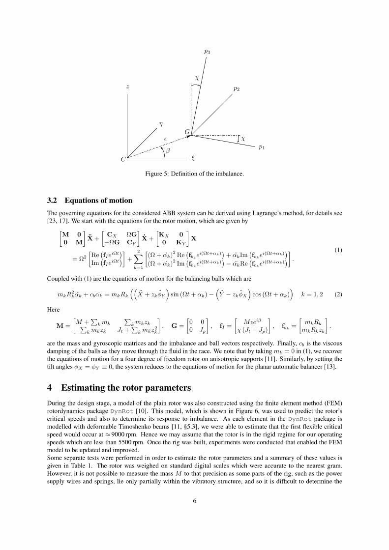
and the spin angle θ0. As the torsional behaviour of the rotor lies outside the scope of the present study, we shall

only consider the special case of constant-speed operation, in which θ0 = Ωt.Next, and as shown in Figure 5, small errors in the rotor’s mass distribution will cause the body axes Cξηz todiffer from the principal axes of the moment of inertia. The eccentricity ǫ, which gives rise to the static imbalance,is defined as the distance between the shaft centre C and the rotor’s centre of mass G. The constant phase withwhich the static imbalance leads the ξ axis is denoted by β. The principal axis p3 corresponding to the polar

moment of inertia may also be misaligned to the shaft axis by an angle χ, and this results in a couple imbalance.We note that the symmetry of the rotor enables the misalignment to be taken about the η axis without detractingfrom the generality of the model.

Finally, the bearings are represented by anisotropic supports which have X and Y as the principal directions ofelasticity. With respect to the vibrational coordinate vector X, the stiffness and damping matrices for this set-up

are given by

K =

[KX 0

0 KY

]

, C =

[CX 0

0 CY

]

.

Here, the X-direction submatrices can be written in terms of the individual support parameters as

KX =

[k1X

+ k2Xk1X

l1 − k2Xl2

k1Xl1 − k2X

l2 k1Xl21 + k2X

l22

]

, CX =

[c1X

+ c2Xc1X

l1 − c2Xl2

c1Xl1 − c2X

l2 c1Xl21 + c2X

l22

]

,

and the expressions for the Y -direction submatrices take the same form.

5

ξ

η

z

ǫ

β

Gχ

χ

p1

p2

p3

C

Figure 5: Definition of the imbalance.

3.2 Equations of motion

The governing equations for the considered ABB system can be derived using Lagrange’s method, for details see

[23, 17]. We start with the equations for the rotor motion, which are given by

[M 0

0 M

]

X +

[CX ΩG

−ΩG CY

]

X +

[KX 0

0 KY

]

X

= Ω2

[Re

(fIe

iΩt)

Im(fIe

iΩt)

]

+

2∑

k=1

[(Ω + αk)

2Re

(fbk

ei(Ωt+αk))

+ αkIm(fbk

ei(Ωt+αk))

(Ω + αk)2Im

(fbk

ei(Ωt+αk))− αkRe

(fbk

ei(Ωt+αk))

]

.

(1)

Coupled with (1) are the equations of motion for the balancing balls which are

mkR2kαk + cbαk = mkRk

((

X + zkφY

)

sin (Ωt + αk) −(

Y − zkφX

)

cos (Ωt + αk))

k = 1, 2 (2)

Here

M =

[M +

∑

k mk

∑

k mkzk∑

k mkzk Jt +∑

k mkz2k

]

, G =

[0 00 Jp

]

, fI =

[Mǫeiβ

χ (Jt − Jp)

]

, fbk=

[mkRk

mkRkzk

]

.

are the mass and gyroscopic matrices and the imbalance and ball vectors respectively. Finally, cb is the viscous

damping of the balls as they move through the fluid in the race. We note that by takingmk = 0 in (1), we recoverthe equations of motion for a four degree of freedom rotor on anisotropic supports [11]. Similarly, by setting the

tilt angles φX = φY ≡ 0, the system reduces to the equations of motion for the planar automatic balancer [13].

4 Estimating the rotor parameters

During the design stage, a model of the plain rotor was also constructed using the finite element method (FEM)

rotordynamics package DynRot [10]. This model, which is shown in Figure 6, was used to predict the rotor’s

critical speeds and also to determine its response to imbalance. As each element in the DynRot package is

modelled with deformable Timoshenko beams [11, §5.3], we were able to estimate that the first flexible critical

speed would occur at ≈ 9000 rpm. Hence we may assume that the rotor is in the rigid regime for our operating

speeds which are less than 5500 rpm. Once the rig was built, experiments were conducted that enabled the FEM

model to be updated and improved.

Some separate tests were performed in order to estimate the rotor parameters and a summary of these values is

given in Table 1. The rotor was weighed on standard digital scales which were accurate to the nearest gram.

However, it is not possible to measure the mass M to that precision as some parts of the rig, such as the power

supply wires and springs, lie only partially within the vibratory structure, and so it is difficult to determine the

6

200150100500−50−100−150−200−100

−50

0

50

100

R

Z (mm)

Y(mm)

RB

Motor

l1l2

B1B2C

z1,2

Disk

Connector Connector

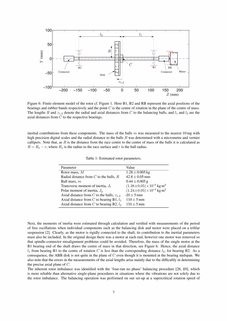
Figure 6: Finite element model of the rotor cf. Figure 1. Here B1, B2 and RB represent the axial positions of the

bearings and rubber bands respectively and the point C is the centre of rotation in the plane of the centre of mass.The lengths R and z1,2 denote the radial and axial distances from C to the balancing balls, and l1 and l2 are theaxial distances from C to the respective bearings.

inertial contributions from these components. The mass of the balls m was measured to the nearest 10mg withhigh precision digital scales and the radial distance to the balls R was determined with a micrometre and verniercallipers. Note that, as R is the distance from the race centre to the centre of mass of the balls it is calculated asR = Rs − r, where Rs is the radius to the race surface and r is the ball radius.

Table 1: Estimated rotor parameters.

Parameter Value

Rotor mass,M 1.28± 0.005 kg

Radial distance from C to the balls, R 42.8± 0.05mm

Ball mass,m 0.44± 0.005 g

Transverse moment of inertia, Jt (1.38±0.05)×10-2 kgm2

Polar moment of inertia, Jp (1.24±0.05)×10-3 kgm2

Axial distance from C to the balls, z1,2 -20± 5mmAxial distance from C to bearing B1, l1 110± 5mm

Axial distance from C to bearing B2, l2 150± 5mm

Next, the moments of inertia were estimated through calculation and verified with measurements of the period

of free oscillations when individual components such as the balancing disk and motor were placed on a trifilar

suspension [2]. Clearly, as the motor is rigidly connected to the shaft, its contribution to the inertial parameters

must also be included. In the original design there was a motor at each end, however one motor was removed so

that spindle-connector misalignment problems could be avoided. Therefore, the mass of the single motor at the

B1 bearing end of the shaft draws the centre of mass in that direction, see Figure 6. Hence, the axial distance

l1 from bearing B1 to the centre of rotation C is less than the corresponding distance l2, for bearing B2. As aconsequence, the ABB disk is not quite in the plane of C even though it is mounted at the bearing midspan. Wealso note that the errors in the measurements of the axial lengths arise mainly due to the difficultly in determining

the precise axial plane of C.The inherent rotor imbalance was identified with the ‘four-run no phase’ balancing procedure [26, §9], which

is more reliable than alternative single-plane procedures in situations where the vibrations are not solely due to

the rotor imbalance. The balancing operation was performed on our set-up at a supercritical rotation speed of

7

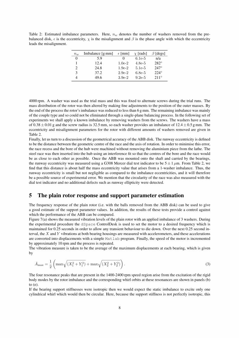
Table 2: Estimated imbalance parameters. Here, nw denotes the number of washers removed from the pre-

balanced disk, ǫ is the eccentricity, χ is the misalignment and β is the phase angle with which the eccentricityleads the misalignment.

nw Imbalance [gmm] ǫ [mm] χ [rads] β [degs]0 5.9 0 6.1e-5 n/a

1 12.4 1.0e-2 4.8e-5 282

2 24.8 1.9e-2 5.1e-5 247

3 37.2 2.9e-2 6.8e-5 224

4 49.6 3.9e-2 9.2e-5 211

4000 rpm. A washer was used as the trial mass and this was fixed to alternate screws during the trial runs. The

mass distribution of the rotor was then altered by making fine adjustments to the position of the outer masses. By

the end of the process the rotor’s imbalance was reduced to less than 6 gmm. The remaining imbalance was mainly

of the couple type and so could not be eliminated through a single-plane balancing process. In the following set of

experiments we shall apply a known imbalance by removing washers from the screws. The washers have a mass

of 0.38± 0.01 g and the screw radius is 32.5mm, so each washer provides an imbalance of 12.4± 0.5 gmm. The

eccentricity and misalignment parameters for the rotor with different amounts of washers removed are given in

Table 2.

Finally, let us turn to a discussion of the geometrical accuracy of the ABB disk. The runway eccentricity is defined

to be the distance between the geometric centre of the race and the axis of rotation. In order to minimise this error,

the race recess and the bore of the hub were machined without removing the aluminium piece from the lathe. The

steel race was then inserted into the hub using an interference fit so that the centres of the bore and the race would

be as close to each other as possible. Once the ABB was mounted onto the shaft and carried by the bearings,

the runway eccentricity was measured using a G308 Mercer dial test indicator to be 5± 1µm. From Table 2, wefind that this distance is about half the mass eccentricity value that arises from a 1-washer imbalance. Thus, the

runway eccentricity is small but not negligible as compared to the imbalance eccentricities, and it will therefore

be a possible source of experimental error. We mention that the circularity of the race was also measured with the

dial test indicator and no additional defects such as runway ellipticity were detected.

5 The plain rotor response and support parameter estimation

The frequency response of the plain rotor (i.e. with the balls removed from the ABB disk) can be used to give

a good estimate of the support parameter values. In addition, the results of these tests provide a control against

which the performance of the ABB can be compared.

Figure 7(a) shows the measured vibration levels of the plain rotor with an applied imbalance of 3 washers. During

the experimental procedure the dSpace ControlDesk is used to set the motor to a desired frequency which is

maintained for 0.25 seconds in order to allow any transient behaviour to die down. Over the next 0.25 second in-

terval, theX and Y vibrations at both bearing housings are measured with accelerometers, and these accelerationsare converted into displacements with a simple Matlab program. Finally, the speed of the motor is incremented

by approximately 10 rpm and the process is repeated.

The vibration measure is taken to be the average of the maximum displacements at each bearing, which is given

by

Amax =1

2

(

max√

(X21 + Y 2

1 ) + max√

(X22 + Y 2

2 )

)

. (3)

The four resonance peaks that are present in the 1400-2400 rpm speed region arise from the excitation of the rigid

body modes by the rotor imbalance and the corresponding whirl orbits at these resonances are shown in panels (b)

to (e).

If the bearing support stiffnesses were isotropic then we would expect the static imbalance to excite only one

cylindrical whirl which would then be circular. Here, because the support stiffness is not perfectly isotropic, this

8

B2D

B1

−0.4

−0.2

0

0.2

−0.4

−0.2

0

0.2

0.4

B2

D

B1

−0.5

0

0.5

−0.5

0

0.5

B2D

B1

−0.5

0

0.5

−0.5

0

0.5

500 1000 1500 2000 2500 3000 3500 4000 4500 50000

0.1

0.2

0.3

0.4

0.5

0.6

B2D

B1

−0.4

−0.2

0

0.2

−0.4

−0.2

0

0.2

0.4

(a)

(b)

(b)

(c)

(c)

(d)

(d) (e)

(e)

X (mm)X (mm)

X (mm)X (mm)

Y(mm)

Y(mm)

Y(mm)

Y(mm)

Am

ax(mm)

Ω (rpm)

Ω = 1415 rpm Ω = 1675 rpm

Ω = 1944 rpm Ω = 2310 rpm

Figure 7: Measured response of the plain rotor with a 3-washer imbalance. Panel (a) shows the lateral vibration

level Amax upon variation of the rotor speed Ω for both the rotor run-up (N) and run-down (). The measuredwhirl orbits at the data points indicated are illustrated in panels (b) to (e). Here B1, B2 and D denote the axial

positions of the bearings and balancing disk respectively. Note that the vibration levels along the length of the

shaft have been inferred from those at the bearings by assuming that the rotor is rigid.

9

B2D

B1

−0.5

0

0.5−0.5

0

0.5

B2D

B1

−0.5

0

0.5−0.5

0

0.5

B2D

B1

−0.2

0

0.2

−0.2

−0.1

0

0.1

0.2

500 1000 1500 2000 2500 3000 3500 4000 4500 5000

0.1

0.2

0.3

0.40.50.6

B2D

B1

−0.2

0

0.2−0.2

−0.1

0

0.1

0.2

(a)

(b)

(b)

(c)

(c)

(d)

(d)

(e)

(e)

X (mm)X (mm)

X (mm)X (mm)

Y(mm)

Y(mm)

Y(mm)

Y(mm)

Am

ax(mm)

Ω (rpm)

Motor resonance

Bearing resonance

Ω = 1455 rpm Ω = 1700 rpm

Ω = 1920 rpm Ω = 2280 rpm

Figure 8: Comparison of the measured response with theory for the plain rotor with a 3-washer imbalance. Panel

(a) shows the log scaled lateral vibration level Amax upon variation of the rotor speed Ω for the rotor run-up (N),run down () and the numerical approximation (- - -). The simulated whirl shapes at the resonance peaks are

illustrated in panels (b) to (e), compare with the experimental results of Figure 7.

10

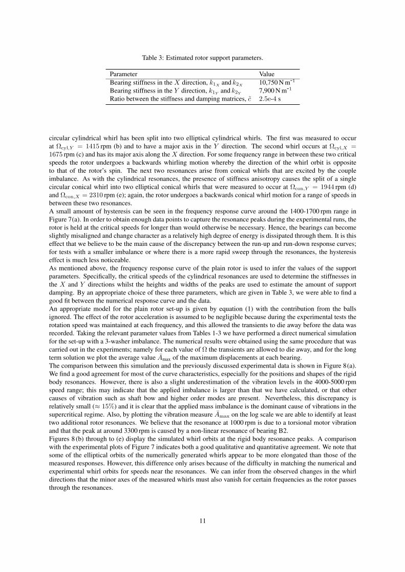
Table 3: Estimated rotor support parameters.

Parameter Value

Bearing stiffness in the X direction, k1Xand k2X

10,750Nm-1

Bearing stiffness in the Y direction, k1Yand k2Y

7,900Nm-1

Ratio between the stiffness and damping matrices, c 2.5e-4 s

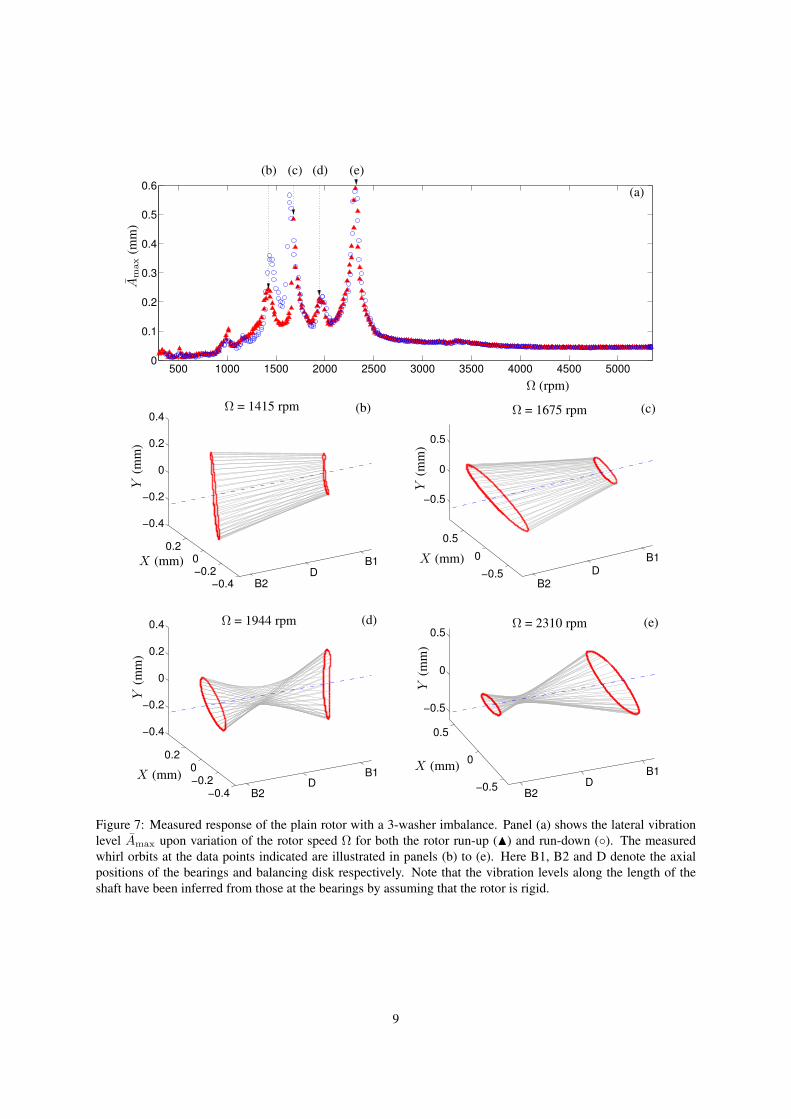
circular cylindrical whirl has been split into two elliptical cylindrical whirls. The first was measured to occur

at Ωcyl,Y = 1415 rpm (b) and to have a major axis in the Y direction. The second whirl occurs at Ωcyl,X =1675 rpm (c) and has its major axis along theX direction. For some frequency range in between these two criticalspeeds the rotor undergoes a backwards whirling motion whereby the direction of the whirl orbit is opposite

to that of the rotor’s spin. The next two resonances arise from conical whirls that are excited by the couple

imbalance. As with the cylindrical resonances, the presence of stiffness anisotropy causes the split of a single

circular conical whirl into two elliptical conical whirls that were measured to occur at Ωcon,Y = 1944 rpm (d)and Ωcon,X = 2310 rpm (e); again, the rotor undergoes a backwards conical whirl motion for a range of speeds inbetween these two resonances.

A small amount of hysteresis can be seen in the frequency response curve around the 1400-1700 rpm range in

Figure 7(a). In order to obtain enough data points to capture the resonance peaks during the experimental runs, the

rotor is held at the critical speeds for longer than would otherwise be necessary. Hence, the bearings can become

slightly misaligned and change character as a relatively high degree of energy is dissipated through them. It is this

effect that we believe to be the main cause of the discrepancy between the run-up and run-down response curves;

for tests with a smaller imbalance or where there is a more rapid sweep through the resonances, the hysteresis

effect is much less noticeable.

As mentioned above, the frequency response curve of the plain rotor is used to infer the values of the support

parameters. Specifically, the critical speeds of the cylindrical resonances are used to determine the stiffnesses in

the X and Y directions whilst the heights and widths of the peaks are used to estimate the amount of supportdamping. By an appropriate choice of these three parameters, which are given in Table 3, we were able to find a

good fit between the numerical response curve and the data.

An appropriate model for the plain rotor set-up is given by equation (1) with the contribution from the balls

ignored. The effect of the rotor acceleration is assumed to be negligible because during the experimental tests the

rotation speed was maintained at each frequency, and this allowed the transients to die away before the data was

recorded. Taking the relevant parameter values from Tables 1-3 we have performed a direct numerical simulation

for the set-up with a 3-washer imbalance. The numerical results were obtained using the same procedure that was

carried out in the experiments; namely for each value of Ω the transients are allowed to die away, and for the longterm solution we plot the average value Amax of the maximum displacements at each bearing.The comparison between this simulation and the previously discussed experimental data is shown in Figure 8(a).

We find a good agreement for most of the curve characteristics, especially for the positions and shapes of the rigid

body resonances. However, there is also a slight underestimation of the vibration levels in the 4000-5000 rpm

speed range; this may indicate that the applied imbalance is larger than that we have calculated, or that other

causes of vibration such as shaft bow and higher order modes are present. Nevertheless, this discrepancy is

relatively small (≈ 15%) and it is clear that the applied mass imbalance is the dominant cause of vibrations in thesupercritical regime. Also, by plotting the vibration measure Amax on the log scale we are able to identify at least

two additional rotor resonances. We believe that the resonance at 1000 rpm is due to a torsional motor vibration

and that the peak at around 3300 rpm is caused by a non-linear resonance of bearing B2.

Figures 8 (b) through to (e) display the simulated whirl orbits at the rigid body resonance peaks. A comparison

with the experimental plots of Figure 7 indicates both a good qualitative and quantitative agreement. We note that

some of the elliptical orbits of the numerically generated whirls appear to be more elongated than those of the

measured responses. However, this difference only arises because of the difficulty in matching the numerical and

experimental whirl orbits for speeds near the resonances. We can infer from the observed changes in the whirl

directions that the minor axes of the measured whirls must also vanish for certain frequencies as the rotor passes

through the resonances.

11

6 The response of the ABB

In this section we build on the results of the plain rotor investigations by considering the response of the two-ball

ABB for a range of different imbalances.

6.1 An applied imbalance of 3 washers

In order for the balls to be added to the rotor, the perspex cover is removed and the balls are placed inside the

disk. At this time we also apply six drops of 10W-40 grade motor oil to the race which provides some damping to

the motion of the balls. The amount of oil is chosen so that the balls are able to overcome gravity and be ‘picked

up’ by the rotation of the race when the disk is spun gently by hand. The cover is then replaced back onto the

disk at the same orientation relative to the hub. During this procedure it is important to minimise any potential

for an unwanted change in the rotor’s imbalance. This is achieved by carefully replacing the screws back into

the holes from where they came and also by tightening them up to the same torque. To aid this operation the

screws and holes are marked with coloured reference stickers, see Figure 2. The estimated change in imbalance

due to the removal and replacement of the cover is estimated to be between 1-2 gmm, which is small compared to

the 12.4± 0.5 gmm imbalance of each applied washer. An alternative to this procedure would be to incorporate

holes in the perspex through which the balls could be placed [27], however this solution was unsuitable for the

considered set-up as oil may have escaped through these openings.

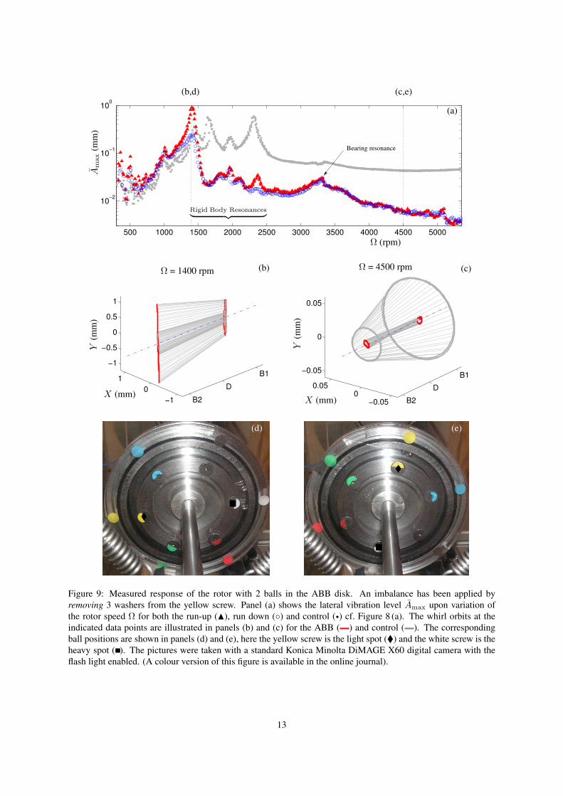
The measured vibration response for the rotor with an applied imbalance of 3 washers and with two balls added

to the ABB disk is illustrated in Figure 9. Panel (a) shows the rotor run-up and run-down compared against the

‘without balls’ control case that was described in the previous section. Here we find that for speeds below the

first resonance the vibration amplitude for the rotor with the balls is increased, whereas, for speeds higher than

this resonance the vibration level is reduced. This automatic balancing effect can be further highlighted through a

comparison of the ball positions and whirl orbits at specific rotation speeds. Panel (b) shows the response during

the rotor run-up at the first rigid body resonance. The whirl shape is the same as that of the control, however, the

amplitude has more than doubled. This occurs because the balancing balls find positions that add to the imbalance,

see panel (d). By contrast, for supercritical speeds the balancing balls move to the opposite side of the race track

(e). Hence, the balls act to reduce the imbalance and the resulting reduction in the vibration amplitude is clearly

evident, see panel (c).

As given in Table 2, the 3-washer imbalance has a magnitude of ≈ 37 gmm. By comparison, each balancing ballhas a mass of 0.44 g and acts at a radius of 42.8mm. Thus, the total imbalance correction capability of the two

balls can be calculated as 2×0.44×42.8 =37.7 gmm. Therefore, to within experimental error, the imbalance ofthe balls matches that of the applied imbalance of the rotor. As a consequence, when the system is in the balanced

state the balls are touching and lie directly in line with the light spot. In fact, a close inspection of Figure 9 (e)

reveals that the balls seem to be forced together with enough pressure that they slide past one another and ride

partway up the groove so that they can occupy close to the same angular position.

A hysteresis effect can be seen in the frequency response curve of Figure 9 (a) around the 1200-1500 rpm and

2200-2500 rpm ranges that contain the first and fourth rigid body resonances respectively. The rotor run-down

has a lower vibration level than the run-up, and for almost all the other test runs the same situation was found.

We believe that this hysteretic behaviour occurs because once the balls have settled at the balanced positions the

subsequent reduction in vibration levels at the critical speeds means that they are less likely to destabilise at the

corresponding resonances on the run-down. In addition, the presence of a small amount of friction between the

balls and the race acts to keep them in the positions that they have found.

As noted during the control study of Section 5, the rotor system possesses a non-linear resonance of the B2 bearing

at around 3300 rpm. We believe that this occurs due to an incorrect installation of the bearing into the housing.

(When installing a bearing it is important to push only on the ring that is being mounted, i.e. on the outer ring

when fitting into a housing and on the inner ring when fitting onto a shaft. Otherwise the rolling elements will be

pushed against the race which could lead to indentations and a damaged bearing). Because the bearing resonance

is not caused by a mass imbalance, the balls are not able to eliminate the vibrations to the same extent that they

have achieved in the higher 4000-5000 rpm operating range. Nevertheless, it is encouraging that the balls aren’t

destabilised by the bearing resonance and that the ABB still effects a reduction in the vibration levels as compared

with the plain rotor control case.

At this point it should be mentioned that the frequency response curves presented in Figure 9 (a) is an example

of a particularly good performance by the ABB. In other test runs there was some variability in the vibration

levels for the ABB in the 1500-3000 rpm range, and these amplitudes were sometimes higher than that of the

12

B2

D

B1

−1

0

1

−1

−0.5

0

0.5

1

B2

D

B1

−0.050

0.05

−0.05

0

0.05

500 1000 1500 2000 2500 3000 3500 4000 4500 5000

10−2

10−1

100

(a)

(b) (c)

(d) (e)

(b,d) (c,e)

Rigid Body Resonances︸ ︷︷ ︸

Bearing resonance

X (mm)X (mm)

Y(mm)

Y(mm)

Am

ax(mm)

Ω (rpm)

Ω = 1400 rpm Ω = 4500 rpm

Figure 9: Measured response of the rotor with 2 balls in the ABB disk. An imbalance has been applied by

removing 3 washers from the yellow screw. Panel (a) shows the lateral vibration level Amax upon variation of

the rotor speed Ω for both the run-up (N), run down () and control (•) cf. Figure 8 (a). The whirl orbits at theindicated data points are illustrated in panels (b) and (c) for the ABB ( ) and control ( ). The corresponding

ball positions are shown in panels (d) and (e), here the yellow screw is the light spot () and the white screw is the

heavy spot ( ). The pictures were taken with a standard Konica Minolta DiMAGE X60 digital camera with the

flash light enabled. (A colour version of this figure is available in the online journal).

13

plain rotor case. Nevertheless, for operating frequencies above 3000 rpm that are supercritical to the rigid body

resonances the vibration levels were consistently reduced and the balls were repeatedly observed in the balanced

state positions. Furthermore, the striking of the base or support structure with a rubber mallet did not move the

balls from those positions, or in other words, the balanced state was found to be robust to external perturbations.

In order to illustrate and support these findings we shall present the results of further tests. However, we shall also

reduce the applied imbalance to 2 washers so that the ABB is not at the limits of its imbalance capability.

6.2 An applied imbalance of 2 washers

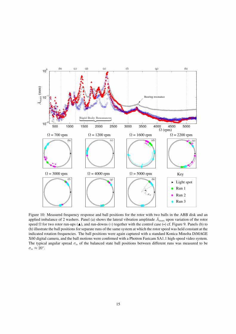
The response of the ABB for an applied imbalance of 2 washers is illustrated in Figure 10. The measured vibration

level for two separate runs are shown in panel (a). During the rotor run-up the vibration level of the ABB is worse

than that of the control case for speeds below the first rigid body resonance. Between the first and last rigid body

resonances the vibration level can either be reduced or increased depending on the specific speed of the rotor.

Nevertheless, at supercritical speeds greater than 3000 rpm the vibration levels of the ABB are consistently less

than that of the plain rotor for both the run-ups and run-downs. As discussed previously, in the 1200-2800 rpm

range the amplitude of vibrations for the rotor run-downs are usually less than that for the corresponding run-

ups. However, in this speed range there can be much variability in the system’s response suggesting that there

is a coexistence between competing states. If we compare the vibration levels of Figures 9 (a) and 10 (a) in the

supercritical range, we find that the vibration levels of the ABB are higher for the reduced imbalance of 2 washers

as compared to the 3-washer case. Again this result was repeatable, however, further discussion as to the possible

reasons for such behaviour will be left until Section 6.3.

First we shall investigate the relationship between the ball positions and the ABB vibration amplitudes. To this

effect, three separate runs were performed where the rotor speed was held constant at certain frequencies of specific

interest. During each run and at each of these speeds three photographs were taken in order to identify the ball

positions. In addition, the ball motions were confirmed with a Photron Fastcam SA1.1 high-speed video system.

Because the bearing housing obscures the field of vision, the photographs could not be taken from an orthogonal

viewpoint, see Figures 9 (d) and (e). Therefore, the photographs are first registered onto an orthogonal base image

by applying a projective transformation using the Matlab ‘Image Processing Toolbox’. The ball angles can

then be determined directly from the transformed photographs, and the estimated error in these measurements is

less than ±2. An alternative procedure would be to apply a protractor, for example via acetate, to the perspexcover. However, the photographs may still need to be registered with an orthogonal base image so as to avoid any

perspective error when reading off the angles.

Figures 10(b) and (c) illustrate that below the first rigid body resonance the balls are positioned on the heavy side

of the rotor and this leads to a greater imbalance and higher vibration levels. At 700 rpm there was some evidence

of periodic motion of the balls but by 1200 rpm they are in a steady state and lie close to the heavy spot.

For speeds between the rigid body resonances there is evidence of a variety of coexisting system behaviours

which causes a variable performance of the ABB in this operating range. Figure 10(d) shows that at 1600 rpm, an

oscillatory touching ball solution coexist with a destabilised solution in which the balls whirl about the race. The

destabilised ball state is accompanied by both a markedly higher vibration amplitude and an audible high pitched

whirring sound that is produced as the balls travel around the race. As the system is rotating in the anti-clockwise

direction we can see that the balls in this state tend to lag behind the rotor when whirling. This is in agreement

with the theory of Ryzhik et al. [20]; there it was found that under certain conditions the balls may stall at a critical

speed and continue to rotate at the eigenfrequency associated with the corresponding mode. Applying those results

to this case we may expect that the balls could stall at Ωcyl,Y ≈ 1450 rpm and remain whirling at this speed evenas the rotor accelerates up to 1600 rpm. However, the determination of the ball speed lies outside the scope of the

present work and we shall leave its study to subsequent investigations. For a higher rotation speed of 2200 rpm,

panel(e), we can see that in two of the runs the balls are split and reside near the balanced state whilst in the other

run there is a motion of the balls within the race. Whether this motion of the balls is periodic, chaotic or transitory

could not be determined. However, it is evident that in the region of the rigid body resonances the behaviour of

the ABB is unpredictable and that the system displays a rich variety of dynamics.

By contrast, for speeds above the rigid body modes the balls consistently find steady state positions that compen-

sate for the imbalance of the rotor, see panels (f), (g) and (h). This leads to a reduced vibration level, and we also

note that the non-linear B2 bearing resonance at 3300 rpm has little effect on the ball positions. Under perfect

conditions, we would expect that the balls would reside in positions such that the angle between them would be

bisected by the light spot. However it was found that the balls were rotated clockwise by between 15-20 fromtheir ideal positions. This discrepancy between the predicted and measured ball positions could arise for a variety

14

500 1000 1500 2000 2500 3000 3500 4000 4500 500010

−2

10−1

100

(b)

(b)

(c)

(c)

(d)

(d)

(e)

(e)

(f)

(f)

(g)

(g)

(h)

(h)

Rigid Body Resonances︸ ︷︷ ︸

Bearing resonance

Am

ax(mm)

Ω (rpm)

Ω = 700 rpm Ω = 1200 rpm Ω = 1600 rpm Ω = 2200 rpm

Ω = 3000 rpm Ω = 4000 rpm Ω = 5000 rpm Key

Light spot

Run 1

Run 2

Run 3

σα

Figure 10: Measured frequency response and ball positions for the rotor with two balls in the ABB disk and an

applied imbalance of 2 washers. Panel (a) shows the lateral vibration amplitude Amax upon variation of the rotor

speed Ω for two rotor run-ups (N), and run-downs () together with the control case (•) cf. Figure 9. Panels (b) to(h) illustrate the ball positions for separate runs of the same system at which the rotor speed was held constant at the

indicated rotation frequencies. The ball positions were again captured with a standard Konica Minolta DiMAGE

X60 digital camera, and the ball motions were confirmed with a Photron Fastcam SA1.1 high-speed video system.

The typical angular spread σα of the balanced state ball positions between different runs was measured to be

σα ≈ 20.

15

of reasons including errors relating to both the runway eccentricity and also to the measurement of the imbalance.

In addition, it can be seen that the balls do not find the exact same positions for the three different runs. We

believe that this behaviour occurs due to the presence of rolling friction between the balls and the race. If the

balls lie within a certain angular range σα then the tangential autobalancing force is not large enough to overcome

the frictional force and the balls remain at the same position. Thus, the effect of friction is to ‘spread out’ the

equilibrium set of the balanced state from two point positions into two intervals on the race. Nevertheless, it is

evident that the ABB reduces the vibration amplitudes for speeds above the rigid body resonances and that this

occurs because the balls consistently find positions at which they act to compensate for the imbalance.

6.3 Further changes to the applied imbalance

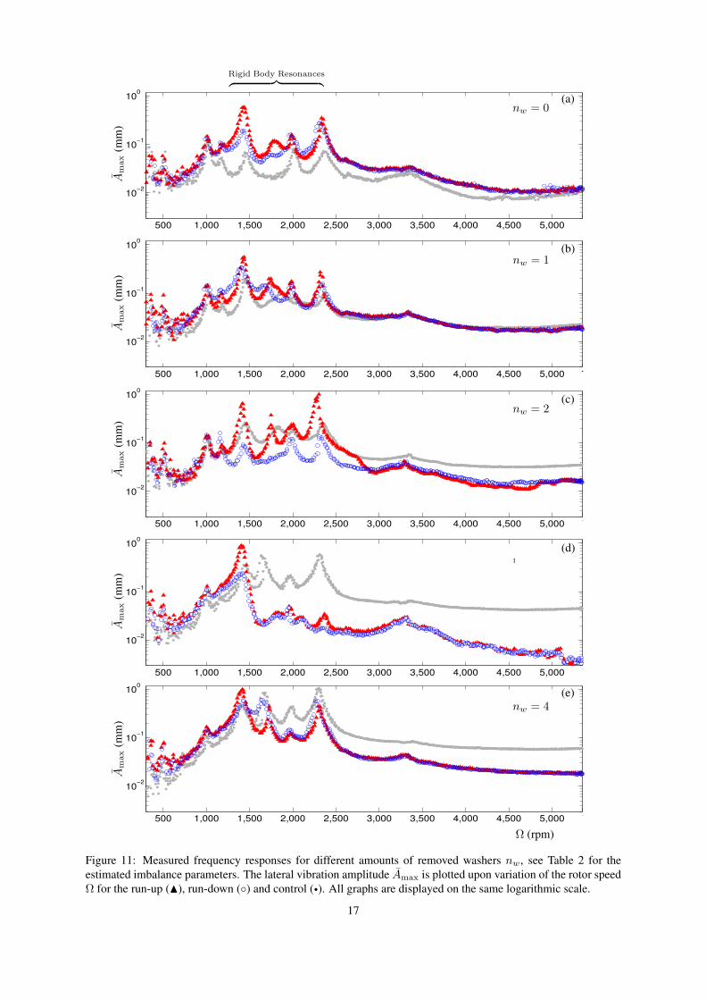
We complete this section by presenting some further frequency response results for different amounts of the ap-

plied imbalance. Figure 11 shows the vibration amplitude as we increase the imbalance from 0 washers (nominally

balanced) up to 4 washers. Most of the common features of the ABB performance have been discussed previously

and we summarise them here as:

1. An increase in the vibration levels for rotation speeds below the first rigid body

resonance.

2. Variable performance in the speed range of the rigid body resonances.

3. Good performance in the frequency range that is supercritical to the rigid body

resonances.

4. Usually the vibration levels are lower on the run down than on the run up.

Figure 12 shows the vibration levels for the different amounts of imbalance during the 4000 to 5000 rpm operating

range. Again, the vibration level for the plain rotor is plotted against the ABB for the rotor run-up and run-down

and the theoretical predictions are shown with the dashed lines. As expected, there is a linear relationship between

the amount of imbalance and the vibration level for the plain rotor. Next, with the balls inside the balancing disk

we find that the ABB does not have much effect on the amplitude of vibration for a 0 or 1 washer imbalance,

however, the vibrations are noticeably reduced for the higher applied imbalances of 2–4 washers. It is also clear

that the ABB performs best with a 3-washer imbalance which is the set-up where the ABB is at the limits of its

balancing capability.

If we were to include the effects of rolling friction into the mathematical model then we would find that the

equilibrium set of the balanced state would ‘spread out’ from point positions, into intervals on the race that are

centred around the desired balanced state [4]. As a consequence, the balls may then have errors in their positions

that are proportional to the amount of rolling friction and it is this effect that we believe is responsible for some

of the discrepancies between the measured and theoretical ABB vibration levels for the cases with 0–2 washer

imbalances.

Applying a similar reasoning, one may assume that the good performance of the ABB for the 3 and 4 washer cases

occurs because the increase in the amount of imbalance helps the balls to overcome the rolling friction force so

that they can reside closer to their desired positions. Also, for these amounts of imbalances the balls are touching,

see Figure 9(e), and they may ride up the race in order to achieve almost exactly the same angular position. More

tests will be needed in order to assess whether the ABB generally performs best when the balancing ball masses

are matched to the rotor imbalance.

7 Comparison with numerical simulations

In this section we compare the results of the experimental ABB investigations with numerical simulations that are

generated from the model that is given by equations (1) and (2). The only parameter that is yet to be considered

is the race damping value cb. This quantity was initially estimated from the decay rate of the motion of a ball as it

was placed on the side of the race and allowed to fall from rest. However, this method leads to a substantial over-

estimation of the value of cb because the oil pools at the bottom of the race and stops the ball almost immediately.

Therefore, as cb is an uncertain quantity we shall produce plots for three different values of the dimensionless race

damping which we define as

cb =cb

mR2Ωcyl,X. (4)

16

500 1,000 1,500 2,000 2,500 3,000 3,500 4,000 4,500 5,000 1

10−2

10−1

100

500 1,000 1,500 2,000 2,500 3,000 3,500 4,000 4,500 5,000 1

10−2

10−1

100

500 1,000 1,500 2,000 2,500 3,000 3,500 4,000 4,500 5,000 1

10−2

10−1

100

500 1,000 1,500 2,000 2,500 3,000 3,500 4,000 4,500 5,000 1

10−2

10−1

100

500 1,000 1,500 2,000 2,500 3,000 3,500 4,000 4,500 5,000 1

10−2

10−1

100

1

(a)

(b)

(c)

(d)

(e)

nw = 0

nw = 1

nw = 2

nw = 4

Rigid Body Resonances︷ ︸︸ ︷

Am

ax(mm)

Am

ax(mm)

Am

ax(mm)

Am

ax(mm)

Am

ax(mm)

Ω (rpm)

Figure 11: Measured frequency responses for different amounts of removed washers nw, see Table 2 for the

estimated imbalance parameters. The lateral vibration amplitude Amax is plotted upon variation of the rotor speed

Ω for the run-up (N), run-down () and control (•). All graphs are displayed on the same logarithmic scale.

17

0 1 2 3 40

0.01

0.02

0.03

0.04

0.05

0.06

0.07

Am

ax(mm)

nw

Figure 12: Vibration amplitudes Amax of the plain rotor (•) and the ABB (N and ) for a different number

of applied washer imbalances nw in the 4000-5000 rpm speed range. The theoretical vibration levels for the

corresponding steady states are shown with the dashed lines.

7.1 An applied imbalance of 3 washers

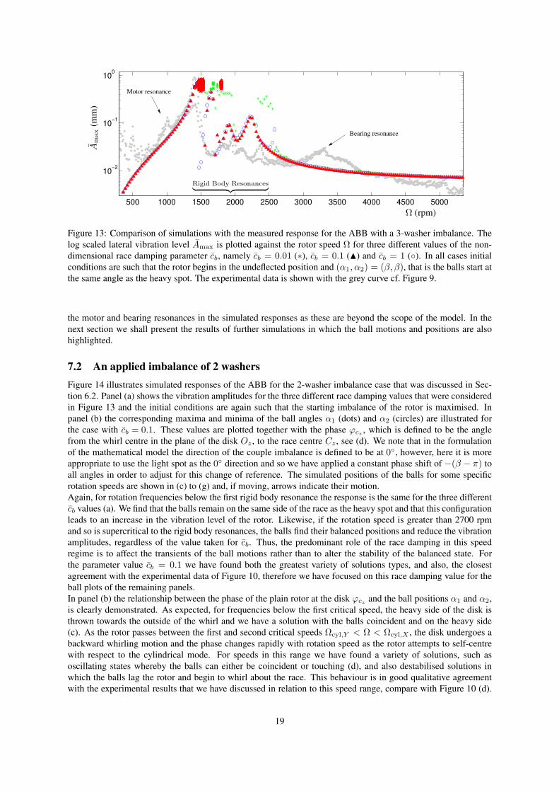
The response of the ABB for the 3-washer imbalance case that was discussed in Section 6.1 is illustrated in

Figure 13. The vibration amplitudes are displayed for three different values of the race damping, namely, cb =0.01,cb = 0.1, and cb = 1. The initial conditions for the system are such that the balls begin at rest with respect to thedisk and in line with the heavy spot, therefore the initial imbalance of the rotor is maximised. For each value of the

rotation speed Ω the system’s response is simulated and after the transients have died away the maximum valuesof the vibration amplitude Amax are plotted.

We find that for speeds below the first rigid body resonance the numerical vibration levels for all values of the race

damping are the same, furthermore these vibration amplitudes agree closely with the experimental results. We

recall that in this subcritical speed range the balls find positions on the heavy side of the rotor and act to maximise

the imbalance.

By contrast, in the frequency range of the rigid body resonances the simulations have different responses that

depend on the amount of race damping. For the low damping value cb = 0.01, we find the highest vibrationlevels. This occurs because in certain speed ranges the balls destabilise and subsequently whirl about the race. For

the other race damping values the vibration amplitudes are again variable, however the qualitative characteristics

of these responses find a better match with the experimental data. It is interesting to note that for this particular

experimental run the ABB has performed better than anticipated. As mentioned in Section 6.1, we believe that this

has occurred because once the balls found their balanced positions after the first resonance, the resulting reduction

in vibration levels meant that they were less likely to destabilise at the subsequent critical speeds. Nevertheless,

other experimental test runs illustrate that the performance of the ABB is highly variable in the 1500-3000 rpm

speed range and so quantitative agreements in this regime should not be expected.

Next, for speeds higher than 3000rpm the simulated steady state responses for all values of the race damping are

the same, and we also find a good quantitative agreement with the experimental results. We recall that in this

frequency regime the balls are positioned on the light side of the rotor and act to minimise the imbalance.

From a design perspective these results are encouraging. We have demonstrated that a good fit to the experimental

data can be achieved with the simple model of (1) and (2). Furthermore, we have found that the determination

of an accurate value for the amount of race damping is not necessary for the prediction of the performance of the

ABB in the supercritical operating frequency regime.

Finally, we note that the rotor run-ups and run-downs have not been included in the considered equations of

motion. This is justified because during the experimental tests the rotation speed was maintained at each frequency,

and so the effect of the torsional acceleration can be assumed to be small. Also, one should not expect to find

18

500 1000 1500 2000 2500 3000 3500 4000 4500 5000

10−2

10−1

100

Am

ax(mm)

Ω (rpm)

Motor resonance

Bearing resonance

Rigid Body Resonances︸ ︷︷ ︸

Figure 13: Comparison of simulations with the measured response for the ABB with a 3-washer imbalance. The

log scaled lateral vibration level Amax is plotted against the rotor speed Ω for three different values of the non-dimensional race damping parameter cb, namely cb = 0.01 (∗), cb = 0.1 (N) and cb = 1 (). In all cases initialconditions are such that the rotor begins in the undeflected position and (α1, α2) = (β, β), that is the balls start atthe same angle as the heavy spot. The experimental data is shown with the grey curve cf. Figure 9.

the motor and bearing resonances in the simulated responses as these are beyond the scope of the model. In the

next section we shall present the results of further simulations in which the ball motions and positions are also

highlighted.

7.2 An applied imbalance of 2 washers

Figure 14 illustrates simulated responses of the ABB for the 2-washer imbalance case that was discussed in Sec-

tion 6.2. Panel (a) shows the vibration amplitudes for the three different race damping values that were considered

in Figure 13 and the initial conditions are again such that the starting imbalance of the rotor is maximised. In

panel (b) the corresponding maxima and minima of the ball angles α1 (dots) and α2 (circles) are illustrated for

the case with cb = 0.1. These values are plotted together with the phase ϕcz, which is defined to be the angle

from the whirl centre in the plane of the disk Oz , to the race centre Cz , see (d). We note that in the formulation

of the mathematical model the direction of the couple imbalance is defined to be at 0, however, here it is moreappropriate to use the light spot as the 0 direction and so we have applied a constant phase shift of −(β − π) toall angles in order to adjust for this change of reference. The simulated positions of the balls for some specific

rotation speeds are shown in (c) to (g) and, if moving, arrows indicate their motion.

Again, for rotation frequencies below the first rigid body resonance the response is the same for the three different

cb values (a). We find that the balls remain on the same side of the race as the heavy spot and that this configuration

leads to an increase in the vibration level of the rotor. Likewise, if the rotation speed is greater than 2700 rpm

and so is supercritical to the rigid body resonances, the balls find their balanced positions and reduce the vibration

amplitudes, regardless of the value taken for cb. Thus, the predominant role of the race damping in this speed

regime is to affect the transients of the ball motions rather than to alter the stability of the balanced state. For

the parameter value cb = 0.1 we have found both the greatest variety of solutions types, and also, the closestagreement with the experimental data of Figure 10, therefore we have focused on this race damping value for the

ball plots of the remaining panels.

In panel (b) the relationship between the phase of the plain rotor at the disk ϕczand the ball positions α1 and α2,

is clearly demonstrated. As expected, for frequencies below the first critical speed, the heavy side of the disk is

thrown towards the outside of the whirl and we have a solution with the balls coincident and on the heavy side

(c). As the rotor passes between the first and second critical speeds Ωcyl,Y < Ω < Ωcyl,X , the disk undergoes a

backward whirling motion and the phase changes rapidly with rotation speed as the rotor attempts to self-centre

with respect to the cylindrical mode. For speeds in this range we have found a variety of solutions, such as

oscillating states whereby the balls can either be coincident or touching (d), and also destabilised solutions in

which the balls lag the rotor and begin to whirl about the race. This behaviour is in good qualitative agreement

with the experimental results that we have discussed in relation to this speed range, compare with Figure 10 (d).

19

500 1000 1500 2000 2500 3000 3500 4000 4500 5000

−100

−50

0

50

100

150

200

500 1000 1500 2000 2500 3000 3500 4000 4500 5000

10−2

10−1

100

Am

ax(mm)

Ω (rpm)

Ω (rpm)

ϕc

z,α

1,α

2

(a)

(b)

(c)

(c)

(d)

(d)

(e)

(e)

(f)

(f)

(g)

(g)

ϕcz

Ω = 1200 rpm Ω ≃ 1600 rpm Ω = 2000 rpm

Ω = 2200 rpm Ω = 4000 rpm Key

Light spot

Whirl centre, O

Race centre, C

O

C

Single ball

Coincident ball

Figure 14: Simulated frequency response and ball positions for the automatic balancer with two balls and an

applied imbalance of 2 washers. Panel (a) shows the lateral vibration amplitude Amax upon variation of the rotor

speed Ω for three different values of the non-dimensional race damping parameter cb, namely cb = 0.01 (∗),cb = 0.1 (N) and cb = 1 (). The control case of the simulated plain rotor is shown by the dashed grey line cf.Figure 10. In panel (b) the ball positions α1 and α2 have been plotted against Ω for the race damping value ofcb = 0.1 and the phase of the disk ϕcz

is also shown for reference. Panels (c) to (g) illustrate the dynamics of

the balls at the specific speeds indicated. Note in panel (d) two distinct observed behaviours are superimposed.

Compare with the experimental results of Figure 10.

20

For frequencies in between 1800 rpm and 2200 rpm, we find that the phase of the rotor approaches near to 0,and so the light side of the disk is brought to the outside of the whirl and the balls find stable positions that are

close to the balanced state (e). We also note that the third resonance at Ωcon,X ≃ 1950 rpm has a relatively smallassociated phase shift, and it is this property of the mode which encourages stable steady state solutions in the

nearby speed range. As the rotor passes through the final rigid body resonance at Ωcon,X ≃ 2310 rpm there isanother change in the phase of the disk as the rotor self-centres with respect to the conical mode. This can lead

to oscillations of the balls about the balanced positions (f) and in some cases they can destabilise completely.

However, for speeds greater than 2300 rpm that are supercritical to the rigid body resonances we find that the light

spot is again brought back to the outside of the whirl and the balls find stable positions that act to balance the disk

(g).

8 Conclusion

The aim of this paper has been to provide a careful experimental validation of the stability properties of automatic

balancers that have recently been analysed theoretically [13, 17]. Such research is clearly vital if automatic

balancers are to become more widely used in practice. At present, the inherent nonlinearity of the ABBmechanism

and its extreme sensitive dependence on frequency and initial conditions have largely precluded their widespread

use in industry. Nevertheless, theory suggests that an ABB will be at its most effective for highly supercritical

rotation speeds, yet this is the region for which the experimental data is the most sparse.

To this effect, we have designed and built an experimental rig that allows the performance of the ball balancer to

be safely observed at rotation frequencies above both the cylindrical and conical rigid body resonances. Once the

rig was built experiments were performed on the plain rotor so that the system parameters could be determined.

It was found that the supports had stiffnesses that were significantly anisotropic, and also that the rotor possessed

an unexpected nonlinear bearing resonance in the supercritical operating range. Nevertheless, a good qualitative

and quantitative description of the plain rotor system was made and these sets of results provided a control against

which the vibration levels of the ABB could be compared.

The performance of the ABB has been assessed for a variety of different applied imbalances for which both the

eccentricity and misalignment of the rotor were taken into account. It was found that for all but the case in

which the rotor was already nominally balanced, the ABB reduced the vibration levels in the speed range that was

supercritical to the rigid body resonances. Some evidence was presented that suggests that the ABB also performs

best when the mass of the balls is matched to to the size of the imbalance. We believe that this behaviour occurs

because the errors in the position of the balls are reduced when they are touching in the balanced state, however,

further tests are needed in order to confirm this hypothesis.

The dynamics of the balancing balls were observed for a specific applied imbalance of 2 washers. As expected, it

was shown that for speeds below the first rigid body resonance the balls cause an increase in the vibration levels by

finding positions on the heavy side of the rotor. By contrast, for speeds supercritical to the rigid body resonances

the balls move to the light side of the rotor and effect a reduction in the vibration levels. In addition, the behaviour

of the ABB for supercritical operating speeds was repeatable and it was found that the balls consistently reside in

positions that were close to the balanced state. Again, the dynamics of the balls during the rigid body resonances

were unpredictable and for this speed range we found a rich variety of system solutions. These included coexist-

ing oscillatory touching ball states, more complex motions where the balls were separated and also destabilised

solutions whereby the balls would whirl about the race and lag behind the speed of the rotor.

In order to accurately describe the behaviour of this ABB system we have used a model that is based on a four

degree of freedom rotor that not only includes the effect of rotor misalignment and eccentricity, but also includes

the effect of support anisotropy. With this model we have established a good agreement between the numerical

simulations and the experimental results. For the supercritical frequency range the model produces an approximate

quantitative match with the measured data and the causes of the discrepancies have been discussed in relation to

both the presence of rolling friction, and also, race eccentricity. During the rigid body resonances the dynamics

of the ABB is highly nonlinear and for this speed range the agreement between theory and experiment is mainly

qualitative. However, the model has been able to successfully reproduce many of the solution types that have been

found experimentally.

The results from this paper have provided both a demonstration of the validity of the mathematical model and

also a ‘proof of concept’ for the feasibility of using an ABB in applications where the rotor is subject to non-

planar tilting vibrations. Future work is needed in order to assess the performance of a corresponding two-plane

automatic balancing mechanism that is capable of fully compensating for both static and couple imbalances.

21

Acknowledgements

DJR gratefully acknowledges the support from a CASE award provided by the EPSRC and Rolls-Royce plc.

References

[1] S. Bae, J. M. Lee, Y. J. Kang, J. S. Kang, and J. R. Yun. Dynamic analysis of an automatic washing machine

with a hydraulic balancer. Journal of Sound and Vibration, 257(1):3–18, 2002.

[2] J. du Bois, N. Lieven, and S. Adhikari. Error analysis in trifilar inertia measurements. Experimental Me-

chanics, 49(4):533–540, 2008.

[3] C.-P. Chao, Y.-D. Huang, and C.-K. Sung. Non-planar dynamic modeling for the optical disk drive spindles

equipped with an automatic balancer. Mechanism and Machine Theory, 38(11):1289–1305, 2003.

[4] C.-P. Chao, C.-K. Sung, and H.-C. Leu. Effects of rolling friction of the balancing balls on the automatic

ball balancer for optical disk drives. Journal of Tribology, 127(4):845–856, 2005.

[5] C.-P. Chao, C.-K. Sung, S.-T. Wu, and J.-S. Huang. Nonplanar modeling and experimental validation of

a spindle–disk system equipped with an automatic balancer system in optical disk drives. Microsystem

Technologies, 13(8-10):1227–1239, 2007.

[6] J. Chung and I. Jang. Dynamic response and stability analysis of an automatic ball balancer for a flexible

rotor. Journal of Sound and Vibration, 259(1):31–43, 2003.

[7] J. Chung and D. S. Ro. Dynamic analysis of an automatic dynamic balancer for rotating mechanisms. Journal

of Sound and Vibration, 228(5):1035–1056, 1999.

[8] dSPACE. http://www.dspaceinc.com, 2010.

[9] ebmpapst. http://www.ebmpapst.com/en/, 2010.

[10] G. Genta. DYNROT: A finite element code for rotordynamic analysis, 2000.

[11] G. Genta. Dynamics of Rotating Systems. Springer, 2005.

[12] K. Green, A. R. Champneys, M. I. Friswell, and A. M. Muñoz. Investigation of a multi-ball, automatic

dynamic balancing mechanism for eccentric rotors. Philosophical Transactions of the Royal Society A:

Mathematical, Physical and Engineering Sciences, 366(1866):705–728, 2008.

[13] K. Green, A. R. Champneys, and N. J. Lieven. Bifurcation analysis of an automatic dynamic balancing

mechanism for eccentric rotors. Journal of Sound and Vibration, 291(3-5):861–881, 2006.

[14] W.-Y. Huang, C.-P. Chao, J.-R. Kang, and C.-K. Sung. The application of ball-type balancers for radial

vibration reduction of high-speed optic disk drives. Journal of Sound and Vibration, 250(3):415–430, 2002.

[15] J. Lee and W. K. Van Moorhem. Analytical and experimental analysis of a self-compensating dynamic

balancer in a rotating mechanism. Journal of Dynamic Systems, Measurement, and Control, 118(3):468–

475, 1996.

[16] C. Rajalingham and S. Rakheja. Whirl suppression in hand-held power tool rotors using guided rolling

balancers. Journal of Sound and Vibration, 217(3):453–466, 1998.

[17] D.J. Rodrigues, A.R. Champneys, M.I. Friswell, and R.E. Wilson. Automatic two-plane balancing for rigid

rotors. International Journal of Non-Linear Mechanics, 43(6):527–541, 2008.

[18] D.J. Rodrigues, A.R. Champneys, M.I. Friswell, and R.E. Wilson. Device asymmetries and the effect of the

rotor run-up in a two-plane automatic ball balancing system. 9th International Conference on Vibrations in

Rotating Machinery, pages 899–907, Exeter, 9-11 September 2008.

22

[19] D.J. Rodrigues, A.R. Champneys, M.I. Friswell, and R.E. Wilson. A consideration of support asymmetry

in an automatic ball balancing system. Sixth EUROMECH Nonlinear Dynamics Conference, ENOC-2008,

Saint Petersburg, Russia, 30 June - 4 July 2008.

[20] B. Ryzhik, L. Sperling, and H. Duckstein. Non-synchronous motions near critical speeds in a single-plane

auto-balancing device. Technische Mechanik, 24:25–36, 2004.

[21] SKF Explorer bearings. http://www.skf.com/files/059281.pdf, 2010.

[22] L. Sperling, B. Ryzhik, and H. Duckstein. Single-plane auto-balancing of rigid rotors. Technische Mechanik,

24:1–24, 2004.

[23] L. Sperling, B. Ryzhik, Ch. Linz, and H. Duckstein. Simulation of two-plane automatic balancing of a rigid

rotor. Math. Comput. Simul., 58(4-6):351–365, 2002.

[24] E. Thearle. A new type of dynamic-balancing machine. Transactions of the ASME, 54(APM-54-12):131–

141, 1932.

[25] N. van de Wouw, M. N. van den Heuvel, H. Nijmeijer, and J. A. van Rooij. Performance of an automatic ball

balancer with dry friction. International Journal of Bifurcation and Chaos, 20(1):65–85, 2005.

[26] V. Wowk. Machinery Vibration: Balancing. McGraw-Hill, 1998.

[27] Q. Yang, E.-H. Ong, J. Sun, G. Guo, and S.-P. Lim. Study on the influence of friction in an automatic ball

balancing system. Journal of Sound and Vibration, 285(1-2):73–99, 2005.

23