Embed Size (px)
Citation preview

Roger Godement
Analysis IIDifferential and Integral Calculus,Fourier Series, Holomorphic Functions
ABC
Roger GodementDépartement de MathématiquesUniversité Paris VII2, place Jussieu75251 Paris Cedex 05FranceE-mail: [email protected]
Translator
Philip SpainMathematics DepartmentUniversity of GlasgowGlasgow G12 8QWScotlandE-mail: [email protected]
Mathematics Subject Classification 2000: 26-01, 26A03, 26A05, 26A09, 26A12, 26A15,26A24, 26A42, 26B05, 28-XX, 30-XX, 30-01, 31-XX, 32-XX, 41-XX, 42-XX, 41-01,43-XX, 44-XX, 54-XX
Library of Congress Control Number: 2003066673
ISBN-10 3-540-20921-2 Springer Berlin Heidelberg New YorkISBN-13 978-3-540-20921-8 Springer Berlin Heidelberg New York
This work is subject to copyright. All rights are reserved, whether the whole or part of the material isconcerned, specifically the rights of translation, reprinting, reuse of illustrations, recitation, broadcasting,reproduction on microfilm or in any other way, and storage in data banks. Duplication of this publicationor parts thereof is permitted only under the provisions of the German Copyright Law of September 9,1965, in its current version, and permission for use must always be obtained from Springer. Violations areliable for prosecution under the German Copyright Law.
Springer is a part of Springer Science+Business Mediaspringeronline.comc© Springer-Verlag Berlin Heidelberg 2005
Printed in The Netherlands
The use of general descriptive names, registered names, trademarks, etc. in this publication does not imply,even in the absence of a specific statement, that such names are exempt from the relevant protective lawsand regulations and therefore free for general use.
Typesetting: by the authors and TechBooks using a Springer LATEX macro package
Cover design: design & production GmbH, Heidelberg
Printed on acid-free paper SPIN: 10866733 41/TechBooks 5 4 3 2 1 0
Contents
V – Differential and Integral Calculus . . . . . . . . . . . . . . . . . . . . . . . . 1§ 1. The Riemann Integral . . . . . . . . . . . . . . . . . . . . . . . . . . . . . . . . . . . 1
1 – Upper and lower integrals of a bounded function . . . . . . . . 12 – Elementary properties of integrals . . . . . . . . . . . . . . . . . . . . . 53 – Riemann sums. The integral notation . . . . . . . . . . . . . . . . . . 144 – Uniform limits of integrable functions . . . . . . . . . . . . . . . . . . 165 – Application to Fourier series and to power series . . . . . . . . 21
§ 2. Integrability Conditions . . . . . . . . . . . . . . . . . . . . . . . . . . . . . . . . . . 266 – The Borel-Lebesgue Theorem . . . . . . . . . . . . . . . . . . . . . . . . . 267 – Integrability of regulated or continuous functions . . . . . . . . 298 – Uniform continuity and its consequences . . . . . . . . . . . . . . . 319 – Differentiation and integration under the
∫sign . . . . . . . . . 36
10 – Semicontinuous functions . . . . . . . . . . . . . . . . . . . . . . . . . . . 4111 – Integration of semicontinuous functions . . . . . . . . . . . . . . . 48
§ 3. The “Fundamental Theorem” (FT) . . . . . . . . . . . . . . . . . . . . . . . . 5212 – The fundamental theorem of the differential and integral
calculus . . . . . . . . . . . . . . . . . . . . . . . . . . . . . . . . . . . . . . . . . 5213 – Extension of the fundamental theorem to regulated func-
tions . . . . . . . . . . . . . . . . . . . . . . . . . . . . . . . . . . . . . . . . . . . . 5914 – Convex functions; Holder and Minkowski inequalities . . . 65
§ 4. Integration by parts . . . . . . . . . . . . . . . . . . . . . . . . . . . . . . . . . . . . . 7415 – Integration by parts . . . . . . . . . . . . . . . . . . . . . . . . . . . . . . . . 7416 – The square wave Fourier series . . . . . . . . . . . . . . . . . . . . . . . 7717 – Wallis’ formula . . . . . . . . . . . . . . . . . . . . . . . . . . . . . . . . . . . . 80
§ 5. Taylor’s Formula . . . . . . . . . . . . . . . . . . . . . . . . . . . . . . . . . . . . . . . . 8218 – Taylor’s Formula . . . . . . . . . . . . . . . . . . . . . . . . . . . . . . . . . . . 82
§ 6. The change of variable formula . . . . . . . . . . . . . . . . . . . . . . . . . . . . 9119 – Change of variable in an integral . . . . . . . . . . . . . . . . . . . . . 9120 – Integration of rational fractions . . . . . . . . . . . . . . . . . . . . . . 95
§ 7. Generalised Riemann integrals . . . . . . . . . . . . . . . . . . . . . . . . . . . . 10221 – Convergent integrals: examples and definitions . . . . . . . . . 10222 – Absolutely convergent integrals . . . . . . . . . . . . . . . . . . . . . . 10423 – Passage to the limit under the
∫sign . . . . . . . . . . . . . . . . . 109
24 – Series and integrals . . . . . . . . . . . . . . . . . . . . . . . . . . . . . . . . . 115
VI Contents
25 – Differentiation under the∫
sign . . . . . . . . . . . . . . . . . . . . . . 11826 – Integration under the
∫sign . . . . . . . . . . . . . . . . . . . . . . . . . 124
§ 8. Approximation Theorems . . . . . . . . . . . . . . . . . . . . . . . . . . . . . . . . 12927 – How to make C∞ a function which is not . . . . . . . . . . . . . 12928 – Approximation by polynomials . . . . . . . . . . . . . . . . . . . . . . . 13529 – Functions having given derivatives at a point . . . . . . . . . . 138
§ 9. Radon measures in R or C . . . . . . . . . . . . . . . . . . . . . . . . . . . . . . . 14130 – Radon measures on a compact set . . . . . . . . . . . . . . . . . . . . 14131 – Measures on a locally compact set . . . . . . . . . . . . . . . . . . . . 15032 – The Stieltjes construction . . . . . . . . . . . . . . . . . . . . . . . . . . . 15733 – Application to double integrals . . . . . . . . . . . . . . . . . . . . . . . 164
§ 10. Schwartz distributions . . . . . . . . . . . . . . . . . . . . . . . . . . . . . . . . . . 16834 – Definition and examples . . . . . . . . . . . . . . . . . . . . . . . . . . . . . 16835 – Derivatives of a distribution . . . . . . . . . . . . . . . . . . . . . . . . . 173
Appendix to Chapter V – Introduction to the Lebesgue Theory179
VI – Asymptotic Analysis . . . . . . . . . . . . . . . . . . . . . . . . . . . . . . . . . . . . 195§ 1. Truncated expansions . . . . . . . . . . . . . . . . . . . . . . . . . . . . . . . . . . . . 195
1 – Comparison relations . . . . . . . . . . . . . . . . . . . . . . . . . . . . . . . . 1952 – Rules of calculation . . . . . . . . . . . . . . . . . . . . . . . . . . . . . . . . . 1973 – Truncated expansions . . . . . . . . . . . . . . . . . . . . . . . . . . . . . . . . 1984 – Truncated expansion of a quotient . . . . . . . . . . . . . . . . . . . . . 2005 – Gauss’ convergence criterion . . . . . . . . . . . . . . . . . . . . . . . . . . 2026 – The hypergeometric series . . . . . . . . . . . . . . . . . . . . . . . . . . . . 2047 – Asymptotic study of the equation xex = t . . . . . . . . . . . . . . 2068 – Asymptotics of the roots of sin x. log x = 1 . . . . . . . . . . . . . 2089 – Kepler’s equation . . . . . . . . . . . . . . . . . . . . . . . . . . . . . . . . . . . 21010 – Asymptotics of the Bessel functions . . . . . . . . . . . . . . . . . . 213
§ 2. Summation formulae . . . . . . . . . . . . . . . . . . . . . . . . . . . . . . . . . . . . 22411 – Cavalieri and the sums 1k + 2k + . . . + nk . . . . . . . . . . . . . 22412 – Jakob Bernoulli . . . . . . . . . . . . . . . . . . . . . . . . . . . . . . . . . . . . 22613 – The power series for cot z . . . . . . . . . . . . . . . . . . . . . . . . . . . 23114 – Euler and the power series for arctanx . . . . . . . . . . . . . . . . 23415 – Euler, Maclaurin and their summation formula . . . . . . . . . 23816 – The Euler-Maclaurin formula with remainder . . . . . . . . . . 23917 – Calculating an integral by the trapezoidal rule . . . . . . . . . 24118 – The sum 1+1/2+ . . .+1/n, the infinite product for the
Γ function, and Stirling’s formula . . . . . . . . . . . . . . . . . . 24219 – Analytic continuation of the zeta function . . . . . . . . . . . . . 247
Contents VII
VII – Harmonic Analysis and Holomorphic Functions . . . . . . . . . 2511 – Cauchy’s integral formula for a circle . . . . . . . . . . . . . . . . . . 251
§ 1. Analysis on the unit circle . . . . . . . . . . . . . . . . . . . . . . . . . . . . . . . . 2552 – Functions and measures on the unit circle . . . . . . . . . . . . . . 2553 – Fourier coefficients . . . . . . . . . . . . . . . . . . . . . . . . . . . . . . . . . . 2614 – Convolution product on T . . . . . . . . . . . . . . . . . . . . . . . . . . . . 2665 – Dirac sequences in T . . . . . . . . . . . . . . . . . . . . . . . . . . . . . . . . 270
§ 2. Elementary theorems on Fourier series . . . . . . . . . . . . . . . . . . . . . 2746 – Absolutely convergent Fourier series . . . . . . . . . . . . . . . . . . . 2747 – Hilbertian calculations . . . . . . . . . . . . . . . . . . . . . . . . . . . . . . . 2758 – The Parseval-Bessel equality . . . . . . . . . . . . . . . . . . . . . . . . . . 2779 – Fourier series of differentiable functions . . . . . . . . . . . . . . . . 28310 – Distributions on T . . . . . . . . . . . . . . . . . . . . . . . . . . . . . . . . . 287
§ 3. Dirichlet’s method. . . . . . . . . . . . . . . . . . . . . . . . . . . . . . . . . . . . . . . 29511 – Dirichlet’s theorem . . . . . . . . . . . . . . . . . . . . . . . . . . . . . . . . . 29512 – Fejer’s theorem . . . . . . . . . . . . . . . . . . . . . . . . . . . . . . . . . . . . 30113 – Uniformly convergent Fourier series . . . . . . . . . . . . . . . . . . . 303
§ 4. Analytic and holomorphic functions . . . . . . . . . . . . . . . . . . . . . . . 30714 – Analyticity of the holomorphic functions . . . . . . . . . . . . . . 30815 – The maximum principle . . . . . . . . . . . . . . . . . . . . . . . . . . . . . 31016 – Functions analytic in an annulus. Singular points. Mero-
morphic functions . . . . . . . . . . . . . . . . . . . . . . . . . . . . . . . . 31317 – Periodic holomorphic functions . . . . . . . . . . . . . . . . . . . . . . 31918 – The theorems of Liouville and of d’Alembert-Gauss . . . . . 32019 – Limits of holomorphic functions . . . . . . . . . . . . . . . . . . . . . . 33020 – Infinite products of holomorphic functions . . . . . . . . . . . . . 332
§ 5. Harmonic functions and Fourier series . . . . . . . . . . . . . . . . . . . . . 34021 – Analytic functions defined by a Cauchy integral . . . . . . . . 34022 – Poisson’s function . . . . . . . . . . . . . . . . . . . . . . . . . . . . . . . . . . 34223 – Applications to Fourier series . . . . . . . . . . . . . . . . . . . . . . . . 34424 – Harmonic functions . . . . . . . . . . . . . . . . . . . . . . . . . . . . . . . . . 34725 – Limits of harmonic functions . . . . . . . . . . . . . . . . . . . . . . . . 35126 – The Dirichlet problem for a disc . . . . . . . . . . . . . . . . . . . . . 354
§ 6. From Fourier series to integrals . . . . . . . . . . . . . . . . . . . . . . . . . . . 35727 – The Poisson summation formula . . . . . . . . . . . . . . . . . . . . . 35728 – Jacobi’s theta function . . . . . . . . . . . . . . . . . . . . . . . . . . . . . . 36129 – Fundamental formulae for the Fourier transform . . . . . . . 36530 – Extensions of the inversion formula . . . . . . . . . . . . . . . . . . . 36931 – The Fourier transform and differentiation . . . . . . . . . . . . . 37432 – Tempered distributions . . . . . . . . . . . . . . . . . . . . . . . . . . . . . 378
Postface. Science, technology, arms . . . . . . . . . . . . . . . . . . . . . . . . . . . 387
Index . . . . . . . . . . . . . . . . . . . . . . . . . . . . . . . . . . . . . . . . . . . . . . . . . . . . . . . . . 436
Table of Contents of Volume I . . . . . . . . . . . . . . . . . . . . . . . . . . . . . . . . 441
V – Differential and Integral Calculus
§ 1. The Riemann integral – § 2. Integrability conditions –§ 3. The “Fundamental Theorem” (FT) – § 4. Integration by parts –§ 5. Taylor’s formula – § 6. The change of variable formula –§ 7.GeneralisedRiemann integrals – § 8.ApproximationTheorems –§ 9. Radon Measures on R or C – § 10. Schwartz distributions
§ 1. The Riemann Integral
The theory of integration expounded in this Chapter dates from the XIXth
century; it was, and remains, of great use in classical mathematics, and itssimplicity has rewarded all who have written for beginners in the subject.For professional mathematicians it has been dethroned by the much morepowerful, and in some respects simpler, theory invented by Henri Lebesguearound 1900, and perfected in the course of the first half of the XXth centuryby dozens of others; we present a small part of it in the Appendix to thisChapter. The “Riemann” theory expounded in this Chapter therefore hasonly a pedagogic interest.
1 – Upper and lower integrals of a bounded function
Let us first recall the definitions of Chap. II, n◦ 11.A scalar (i.e. complex-valued) function ϕ defined on a compact, or more
generally, bounded, interval I is said to be a step function if one can find apartition (Chap. I) of I into a finite number of intervals Ik such that ϕ isconstant on each Ik; no conditions are imposed on the Ik. Such a partitionwill be said to be adapted to ϕ.
When I = (a, b) this is the same as requiring the existence of a finitesequence of points of I satisfying
a = x1 ≤ x2 ≤ . . . ≤ xn+1 = b(1.1)
and such that ϕ is constant on each open interval ]xk, xk+1[, because thevalues it takes at a point xk have no connection with those it takes to the
2 V – Differential and Integral Calculus
right or left of this point, and are irrelevant to the calculation of traditionalintegrals1.
A sequence of points satisfying (1) is called a subdivision of the interval I.A subdivision by the points yh is said to be finer than the subdivision (1)when the xk appear among the yh, in other words when the second subdivi-sion is obtained by subdividing each of the component intervals in (1). Thedefinition is similar for two partitions (Ik) and (Jh) of I: the second is saidto be finer than the first if every Jh is contained in one of the Ik, in otherwords if the second partition of I is obtained by partitioning each of the Ik
themselves into intervals (namely, those Jh contained in Ik).If ϕ(x) = ak for every x ∈ Ik one calls the number
m(ϕ) =∑
akm(Ik) =∑
ϕ(ξk)m(Ik)(1.2)
the integral of ϕ over I, where, for every interval J = (u, v), the numberm(J) = v − u denotes the length or measure of J , and where ξk is any pointof Ik. Since the Ik of zero measure do not matter in (2) one can replace thepartition by a subdivision (1) and write
m(ϕ) =∑
ϕ(ξk)(xk+1 − xk) with xk < ξk < xk+1(1.3)
since ϕ is constant, so equal to ϕ(ξk), on ]xk, xk+1[.Since there are infinitely many ways of choosing the Ik – every finer
partition, for example, will equally be adapted to calculating the integral –,we have to show that the sum (2) does not depend on the choice of the Ik. Solet (Jh) be another partition of I into intervals such that ϕ(x) = bh for everyx ∈ Jh. Since each Ik is the union of the pairwise disjoint intervals Ik ∩ Jh,as is shown by the relation
X = X ∩ I = X ∩⋃
Jh =⋃
X ∩ Jh,
valid for every subset X of I, we have
m(Ik) =∑
h
m(Ik ∩ Jh)
and similarlym(Jh) =
∑k
m(Ik ∩ Jh)
where, by convention, m(∅) = 0. Thus∑akm(Ik) =
∑akm(Ik ∩ Jh),(1.4) ∑
bhm(Jh) =∑
bhm(Ik ∩ Jh),(1.5)
1 This is not the same in generalisations of the classical theory. See n◦ 30.
§ 1. The Riemann Integral 3
where, on the right hand sides, we sum over all the pairs (k, h). We thus haveonly to prove that
m(Ik ∩ Jh) �= 0 implies ak = bh,
which is clear: on Ik ∩ Jh, which is nonempty since its length is not zero, thefunction ϕ is equal simultaneously to ak and to bh.
This argument shows immediately that
m(λϕ + µψ) = λm(ϕ) + µm(ψ)(1.6)
for any step functions ϕ and ψ and constants λ and µ: consider partitions(Ik) and (Jh) of I adapted to ϕ and ψ, write ak for the value of ϕ on Ik andbh for that of ψ on Jh, and calculate the integrals of ϕ, ψ and λϕ+µψ usingthe intervals Ik ∩Jh on which ϕ, ψ and λϕ+µψ are equal respectively to ak,bh and λak +µbh; in effect we are adding the relations (4) and (5), multipliedrespectively by λ and µ, term-by-term.
Since it is clear that the integral of a positive function (i.e. one whosevalues are all positive) is positive, we see that
ϕ ≤ ψ implies m(ϕ) ≤ m(ψ)(1.7)
for real-valued ϕ and ψ, since m(ψ)−m(ϕ) = m(ψ−ϕ) ≥ 0 by (6) and ψ−ϕis positive.
Finally, the triangle inequality applied to (2) shows that
|m(ϕ)| ≤∑
|ϕ(ξk)|m(Ik) = m(|ϕ|) ≤∑
‖ϕ‖Im(Ik)
always, where, as in Chap. III, n◦ 7, we write in a general way that
‖f‖I = supx∈I
|f(x)|.
Since∑
m(Ik) = m(I) we finally obtain the inequality
|m(ϕ)| ≤ m(|ϕ|) ≤ m(I)‖ϕ‖I .(1.8)
This completes the “theory” of integration as it applies to step functions.It rests on two properties of lengths which are the starting point for all latergeneralisations:
(M 1): the measure of an interval is positive;(M 2): measure is additive, i.e. if an interval J is the union of a finite number
of pairwise disjoint intervals Jk then m(J) =∑
m(Jk).
There are many other interval-functions which have these properties. Onecan, for example, choose a continuous function µ(x) which is increasing inthe wide sense on I and put2
2 For an arbitrary increasing function one has to take account of its discontinuitiesand modify the formula to obtain a reasonable theory. See n◦ 32 on Stieltjesmeasures.
4 V – Differential and Integral Calculus
µ(J) = µ(v) − µ(u) if J = (u, v).
One can also take a finite or countable set D ⊂ I and assign to each ξ ∈ Da “mass” c(ξ) > 0, with
∑c(ξ) < +∞, and then put
µ(J) =∑ξ∈J
c(ξ)
for every interval J , so that the measure of a singleton interval can very wellbe > 0; in this example property (M 2) reduces to the associativity formulafor absolutely convergent series. We obtain discrete measures in this way.
For a “measure” µ satisfying (M 1) and (M 2) the integral of a step func-tion is, by definition, the number µ(ϕ) given by the formula (2), replacingthe letter m by the letter µ. For a discrete measure, one clearly finds thatµ(ϕ) =
∑c(ξ)ϕ(ξ), summing over all the ξ ∈ D. These generalisations will
be studied at the end of this chapter, but the reader may be interested to ob-serve, every time we use the traditional integral, those results which dependonly on the properties (M 1) and (M 2) of “Euclidean” or “Archimedean”measure, or, as one now calls it, of “Lebesgue measure” (since it was forthis that Lebesgue constructed his grand integration theory) because theseproperties extend to the general case. Certain results which, on the contrary,use the explicit construction starting from the usual measure, mainly concernthe relations between integrals and derivatives, Fourier series and integrals,partial differential equations, almost all applications to physical sciences, etc.They rest on an obvious though fundamental property of the usual measure:it is invariant under translation; see below, (2.20).
Now let us pass on to arbitrary bounded real functions on a boundedinterval I (in general compact).
Given a bounded real-valued function f on I there exist step functions,even constant functions, ϕ and ψ, such that ϕ ≤ f ≤ ψ, i.e. ϕ(x) ≤ f(x) ≤ψ(x) for every x ∈ I. By (7) we must have m(ϕ) ≤ m(ψ), and every rea-sonable definition of m(f) must satisfy m(ϕ) ≤ m(f) ≤ m(ψ). We thereforeexamine the lower and upper integrals of f over I defined by the formulae
m∗(f) = supϕ≤f
m(ϕ), m∗(f) = infψ≥f
m(ψ)(1.9)
where ϕ and ψ range over the sets of step functions such that ϕ ≤ f ≤ ψ.As we have seen in Chap. II, n◦ 11, we have m∗(f) ≤ m∗(f) since every
number m(ϕ) is less than the m(ψ), so is less than their lower bound m∗(f),which, larger than all the m(ϕ), is also larger than their upper bound m∗(f).Since the constant functions equal to −‖f‖I and +‖f‖I feature among thefunctions ϕ and ψ respectively, we even have
−m(I)‖f‖I ≤ m∗(f) ≤ m∗(f) ≤ m(I)‖f‖I .(1.10)
§ 1. The Riemann Integral 5
Relation (6) does not extend to the lower and upper integrals of arbitraryfunctions; if it did, the theory of integration would finish with n◦ 2 of thischapter. However, we always have the inequalities
m∗(f + g) ≥ m∗(f) + m∗(g), m∗(f + g) ≤ m∗(f) + m∗(g).(1.11)
Among the step functions less than f + g are the sums ϕ+ψ, where ϕ is lessthan f and where ψ is less than g; consequently, m∗(f + g) is greater thanall the numbers of the form m(ϕ + ψ) = m(ϕ) + m(ψ). It remains to notethat if A and B are two sets of real numbers, and if one writes A+B for theset of numbers x + y where x ∈ A and y ∈ B, then
sup(A + B) = sup(A) + sup(B)
with a similar relation for the lower bounds (exercise!), so that every numberlarger than the x+y is larger than sup(A)+sup(B). Whence the first relation(11). The second is proved in the same way, reversing the inequalities.
It is easier to show that
m∗(cf) = cm∗(f), m∗(cf) = cm∗(f) for every c ≥ 0(1.12)
and
m∗(−f) = −m∗(f);(1.13)
it is enough to note that multiplication by −1 transforms the step functionsbelow f into those above −f .
2 – Elementary properties of integrals
The most natural definition of integrable functions with real values is thatthey should satisfy the condition
m∗(f) = m∗(f),
the common value of the two sides then being the value of the integral m(f)of f ; one extends the definition to functions f = g + ih with complex valuesby requiring both g and h to be integrable and putting
m(f) = m(g) + im(h).
This definition, adopted in the First French Edition for reasons of simplicity,has several drawbacks; in particular, it is not obvious — although, of course,true — that the absolute value |f | = [Re(f)2+Im(f)2]
12 of a complex-valued
integrable function is again integrable, as Michel Ollitrault, a reader of theFirst Edition, has justly remarked to me. We shall therefore abandon thisdefinition temporarily, to recover it later, and we shall adopt a method used
6 V – Differential and Integral Calculus
in the modern theory too. We shall develop it for complex-valued functions,but it will also apply to functions with values in a finite dimensional vectorspace, or even a Banach space, which is not the case for the first simplisticdefinition.
We shall say that a function f is integrable if, for any r > 0, there isa step function ϕ (with values in the same space as f if one is integratingvector-valued functions) such that
m∗(|f − ϕ|) < r.(2.1)
If f has real values this means, intuitively, that the numerical (and not al-gebraic) measure of the area in the plane included between the graphs of fand ϕ is < r; there is no point in assuming ϕ “above” or “below” f . It comesto the same to require the existence of a sequence of step functions ϕn suchthat
limm∗(|f − ϕn|) = 0(2.1’)
or, as one says, which converges in mean to f . One says “in mean” becausethe fact that the upper integral of a positive function h(x) is very smalldoes not prevent h from taking very large values on very small intervals:1010010−200 = 10−100.
To define the integral of an integrable function f one uses the relation(1’). By the triangle inequality we have
|ϕp − ϕq| ≤ |ϕp − f | + |f − ϕq|and so
|m(ϕp) − m(ϕq)| = |m(ϕp − ϕq)| ≤ m∗(|ϕp − f |) + m∗(|f − ϕq|),by (1.11). The sequence with general term m(ϕn) therefore satisfies Cauchy’sconvergence criterion (Chap. III, n◦ 10, Theorem 13). Its limit depends onlyon f . For if ψn is another sequence of step functions satisfying (1’) the relation
|ϕn − ψn| ≤ |f − ϕn| + |f − ψn|shows, in a similar way, that m(ϕn) − m(ψn) tends to 0.
It is natural to call the limit of the m(ϕn) (common to all sequences ofstep functions converging to f in mean) the integral of f , and to denote it bym(f). This kind of argument, used in many other places, is similar to the onewe used to define ax for a > 0 and x ∈ R, by approximating x by a sequenceof rational numbers xn and showing that the sequence axn converges to alimit independent of x (Chapter IV, § 1, end of n◦ 2).
If an integrable function f has real (resp. positive) values then its integralis real (resp. positive). If f is real, and if in (1’) one replaces ϕn by Re ϕn
one decreases the function |f − ϕn| and so its upper integral, so that the
§ 1. The Riemann Integral 7
sequence of real functions Re(ϕn) again converges to f in mean, whence thefirst result. If, moreover, f is positive, in which case one may assume the ϕn
real, one argues in the same way, replacing the ϕn(x) by 0 on the intervalswhere ϕn < 0: this can only decrease the value of |f(x) − ϕn(x)|, and so ofthe upper integral.
If f and g are integrable then f + g is integrable and
m(f + g) = m(f) + m(g).
Take step functions ϕn and ψn converging in mean to f and g, write
|(f + g) − (ϕn + ψn)| ≤ |f − ϕn| + |g − ψn|
to show that ϕn + ψn converges to f + g in mean, and use (1.6).If f is integrable then so is αf for any α ∈ C, and m(αf) = αm(f).
Obvious: multiply f and ϕ by α in (1) and apply (1.12).These first results already show, for real integrable f and g, that
f ≤ g implies m(f) ≤ m(g),
since 0 ≤ m(g − f) = m(g) + m(−f) = m(g) − m(f).If f is integrable then so is |f |, and
|m(f)| ≤ m(|f |) ≤ m(I) ‖f‖I(2.2)
where, we recall, ‖f‖I = sup |f(x)| is the norm of uniform convergence on I(Chap. III, n◦ 7). For any complex numbers α and β we have
∣∣|α| − |β|∣∣ ≤|α − β|, whence, in the notation of (1’),∣∣|f(x)| − |ϕn(x)|∣∣ ≤ |f(x) − ϕn(x)| for all x ∈ I
and so m∗(|f | − |ϕn|) ≤ m∗(|f − ϕn|); this proves that |f | is integrable likef , since the |ϕn| are also step functions. Since the integrals of ϕn and |ϕn|converge to those of f and |f |, by definition of the latter, and since (2) appliesto the ϕn, one obtains the first inequality (2) in the limit. The second followsfrom the fact that |f(x)| ≤ ‖f‖I everywhere on I, so that m(|f |) is less thanthe integral of the constant function x → ‖f‖I .
The complex-valued function f is integrable if and only if the functionsRe(f) and Im(f) are. If so,
m(f) = m[Re(f)] + i.m[Im(f)].
Since |Re(f) − Re(ϕn)| ≤ |f − ϕn|, with a similar relation for the imaginaryparts, it is clear that Re(f) and Im(f) are integrable if f is; the relation tobe shown then follows from the linearity properties already obtained; theseshow no less trivially that f is integrable if Re(f) and Im(f) are.
8 V – Differential and Integral Calculus
A real function f is integrable if and only if m∗(f) = m∗(f).Suppose first that m∗(f) = m∗(f). Then, for every r > 0 there are step
functions ϕ and ψ framing f whose integrals are equal to within r. Since|f −ψ| = f −ψ ≤ ϕ−ψ it follows that m∗(|f −ψ|) ≤ m(ϕ−ψ) < r, whencethe integrability of f .
Suppose conversely that f is integrable and consider a step function ϕsuch that
m∗(|f − ϕ|) < r;
one may assume ϕ real as above. Since m∗(|f −ϕ|) is, by definition, the lowerbound of the numbers m(ψ) over all step functions ψ ≥ |f − ϕ|, the strictinequality proves the existence of a step function ψ such that
|f − ϕ| < ψ & m(ψ) < r.
Since ϕ− ψ ≤ f ≤ ϕ + ψ we have thus framed f between two step functionswhose difference has integral ≤ 2r; so m∗(f) = m∗(f). Moreover,
m(ϕ − ψ) ≤ m∗(f) ≤ m(ϕ + ψ);
since f is integrable we already know that this relation is preserved if onereplaces m∗(f) by m(f), whence m(f) = m∗(f), since the extreme terms inthe preceding relation are equal to within 2r.
To sum up:
Theorem 1. Let I be a bounded interval. (i) If the bounded functions f andg are integrable on I, then so likewise is αf + βg for any constants α and β,and
m(αf + βg) = αm(f) + βm(g).(2.3)
(ii) If f is defined, bounded and integrable on I, then the function |f | isintegrable, and
|m(f)| ≤ m(|f |) ≤ m(I)‖f‖I = m(I). sup |f(x)|.(2.4)
(iii) The integral of a positive function is positive.
The standard notation
m(f) =∫
I
f(x)dx
will be explained later (n◦ 3).The definition of integrable functions shows immediately that, on a com-
pact interval, every regulated function is integrable; for every r > 0 thereexists, by the definition (Chap. III, n◦ 12) a step function ϕ such that|f(x) − ϕ(x)| < r for every x; then, by (1.10), m∗(|f − ϕ|) < m(I)r, whence
§ 1. The Riemann Integral 9
the result. We shall prove later (n◦ 7) that, on a compact interval, every con-tinuous function is regulated, so integrable. One hardly needs more subtleresults in elementary analysis.
It is not difficult to construct non-integrable functions: it is enough totake the Dirichlet function f(x) on I, equal to 0 if x ∈ Q and to 1 if x /∈ Q.Now, if a step function ϕ ≤ f is constant on the intervals Ik of a partitionof I, it must be ≤ 0 on every nonsingleton Ik since such an interval containsrational numbers where f(x) = 0; likewise, every step function ψ ≥ f must be“almost” everywhere ≥ 1. Thus m∗(f) = 0 and m∗(f) = m(I). The Lebesguetheory allows one to integrate the function f , with the same result as if onehad f(x) = 1 everywhere, and this because Q is countable. It may appearbizarre to consider such functions – Newton would have said that one doesnot meet them in Nature3 –, but it is one of those which led Cantor towardshis great set theory, not to be confused with the trivialities of Chap. I. Eventhough the function in question is strange, one cannot deny it the merit ofsimplicity; if analysis is incapable of integrating such functions, one mightbegin to suspect that this is the fault of analysis and not of the function . . .
We said above that the integral of a positive function is positive; could itperhaps be zero? This is one of the fundamental questions which the completeLebesgue theory allows one to resolve. For the moment we make just twoelementary remarks.
If the integral of a continuous positive function f is zero, then f = 0. Forif we have f(a) = r > 0 for some a ∈ I, then the continuity of f shows thatf(x) > r/2 on an interval J ⊂ I of length > 0; if ϕ is the step function equalto r/2 on J and to 0 elsewhere then m(f) ≥ m(ϕ) = r m(J)/2 > 0.
This result (which presupposes the integrability of the continuous func-tions and uses the fact that, in the traditional theory, the measure of a non-empty open interval is > 0) does not extend to discontinuous functions. For apositive step function for example, it is clear that the integral vanishes if andonly if the points where the function does not vanish are finite in number. Inthe much more general case of a regulated function, the apposite conditionis that the set defined by the relation f(x) �= 0 should be countable (n◦ 7).
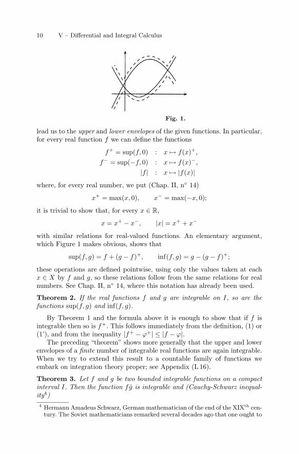
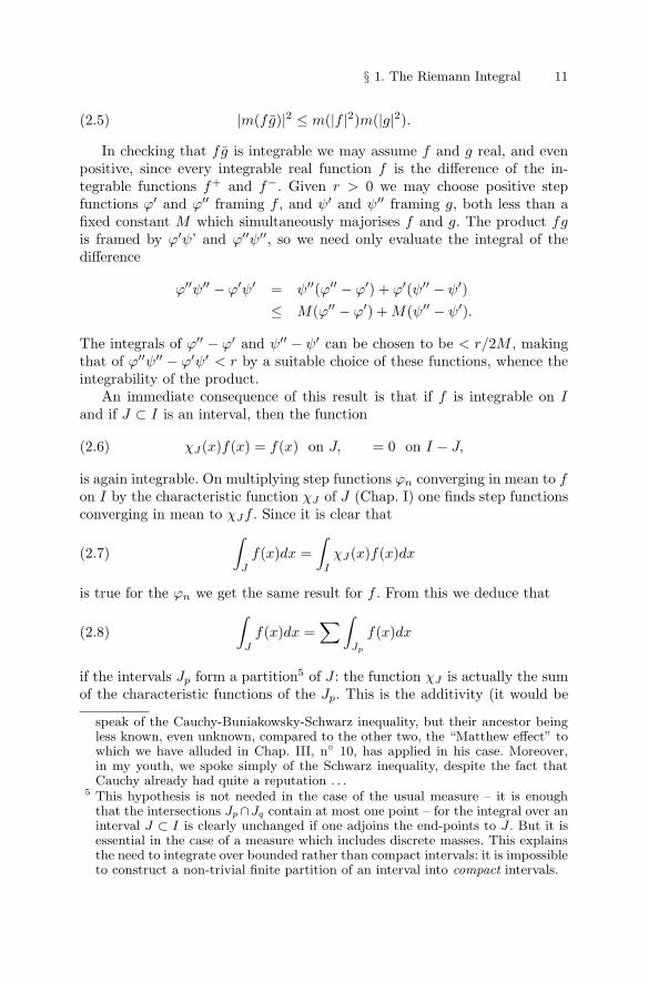
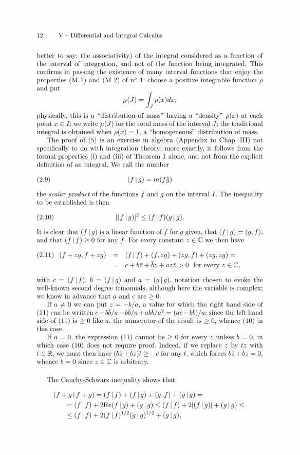
Before stating the next theorem let us note that if we have real functionsf and g defined on any set X we can construct the functions
sup(f, g) : x → max[f(x), g(x)],inf(f, g) : x → min[f(x), g(x)];
these definitions generalise in the obvious way to a finite number of functions(and even to an infinite number on replacing max and min by sup and inf) and
3 We will meet them in computer science when there exist machines capable ofdistinguishing the rational numbers automatically from the others.
10 V – Differential and Integral Calculus
Fig. 1.
lead us to the upper and lower envelopes of the given functions. In particular,for every real function f we can define the functions
f+ = sup(f, 0) : x → f(x)+,
f− = sup(−f, 0) : x → f(x)−,
|f | : x → |f(x)|where, for every real number, we put (Chap. II, n◦ 14)
x+ = max(x, 0), x− = max(−x, 0);
it is trivial to show that, for every x ∈ R,
x = x+ − x−, |x| = x+ + x−
with similar relations for real-valued functions. An elementary argument,which Figure 1 makes obvious, shows that
sup(f, g) = f + (g − f)+, inf(f, g) = g − (g − f)+;
these operations are defined pointwise, using only the values taken at eachx ∈ X by f and g, so these relations follow from the same relations for realnumbers. See Chap. II, n◦ 14, where this notation has already been used.
Theorem 2. If the real functions f and g are integrable on I, so are thefunctions sup(f, g) and inf(f, g).
By Theorem 1 and the formula above it is enough to show that if f isintegrable then so is f+. This follows immediately from the definition, (1) or(1’), and from the inequality |f+ − ϕ+| ≤ |f − ϕ|.
The preceding “theorem” shows more generally that the upper and lowerenvelopes of a finite number of integrable real functions are again integrable.When we try to extend this result to a countable family of functions weembark on integration theory proper; see Appendix (L 16).
Theorem 3. Let f and g be two bounded integrable functions on a compactinterval I. Then the function fg is integrable and (Cauchy-Schwarz inequal-ity4)4 Hermann Amadeus Schwarz, German mathematician of the end of the XIXth cen-
tury. The Soviet mathematicians remarked several decades ago that one ought to
§ 1. The Riemann Integral 11
|m(fg)|2 ≤ m(|f |2)m(|g|2).(2.5)
In checking that fg is integrable we may assume f and g real, and evenpositive, since every integrable real function f is the difference of the in-tegrable functions f+ and f−. Given r > 0 we may choose positive stepfunctions ϕ′ and ϕ′′ framing f , and ψ′ and ψ′′ framing g, both less than afixed constant M which simultaneously majorises f and g. The product fgis framed by ϕ′ψ’ and ϕ′′ψ′′, so we need only evaluate the integral of thedifference
ϕ′′ψ′′ − ϕ′ψ′ = ψ′′(ϕ′′ − ϕ′) + ϕ′(ψ′′ − ψ′)≤ M(ϕ′′ − ϕ′) + M(ψ′′ − ψ′).
The integrals of ϕ′′ − ϕ′ and ψ′′ − ψ′ can be chosen to be < r/2M , makingthat of ϕ′′ψ′′ − ϕ′ψ′ < r by a suitable choice of these functions, whence theintegrability of the product.
An immediate consequence of this result is that if f is integrable on Iand if J ⊂ I is an interval, then the function
χJ(x)f(x) = f(x) on J, = 0 on I − J,(2.6)
is again integrable. On multiplying step functions ϕn converging in mean to fon I by the characteristic function χJ of J (Chap. I) one finds step functionsconverging in mean to χJf . Since it is clear that∫
J
f(x)dx =∫
I
χJ(x)f(x)dx(2.7)
is true for the ϕn we get the same result for f . From this we deduce that∫J
f(x)dx =∑∫
Jp
f(x)dx(2.8)
if the intervals Jp form a partition5 of J : the function χJ is actually the sumof the characteristic functions of the Jp. This is the additivity (it would be
speak of the Cauchy-Buniakowsky-Schwarz inequality, but their ancestor beingless known, even unknown, compared to the other two, the “Matthew effect” towhich we have alluded in Chap. III, n◦ 10, has applied in his case. Moreover,in my youth, we spoke simply of the Schwarz inequality, despite the fact thatCauchy already had quite a reputation . . .
5 This hypothesis is not needed in the case of the usual measure – it is enoughthat the intersections Jp∩Jq contain at most one point – for the integral over aninterval J ⊂ I is clearly unchanged if one adjoins the end-points to J . But it isessential in the case of a measure which includes discrete masses. This explainsthe need to integrate over bounded rather than compact intervals: it is impossibleto construct a non-trivial finite partition of an interval into compact intervals.
12 V – Differential and Integral Calculus
better to say: the associativity) of the integral considered as a function ofthe interval of integration, and not of the function being integrated. Thisconfirms in passing the existence of many interval functions that enjoy theproperties (M 1) and (M 2) of n◦ 1: choose a positive integrable function ρand put
µ(J) =∫
J
ρ(x)dx;
physically, this is a “distribution of mass” having a “density” ρ(x) at eachpoint x ∈ I; we write µ(J) for the total mass of the interval J ; the traditionalintegral is obtained when ρ(x) = 1, a “homogeneous” distribution of mass.
The proof of (5) is an exercise in algebra (Appendix to Chap. III) notspecifically to do with integration theory; more exactly, it follows from theformal properties (i) and (iii) of Theorem 1 alone, and not from the explicitdefinition of an integral. We call the number
(f | g) = m(fg)(2.9)
the scalar product of the functions f and g on the interval I. The inequalityto be established is then
|(f | g)|2 ≤ (f | f)(g | g).(2.10)
It is clear that (f | g) is a linear function of f for g given, that (f | g) = (g, f),and that (f | f) ≥ 0 for any f . For every constant z ∈ C we then have
(f + zg, f + zg) = (f | f) + (f, zg) + (zg, f) + (zg, zg) =(2.11)= c + bz + bz + azz > 0 for every z ∈ C,
with c = (f | f), b = (f | g) and a = (g | g), notation chosen to evoke thewell-known second degree trinomials, although here the variable is complex;we know in advance that a and c are ≥ 0.
If a �= 0 we can put z = −b/a, a value for which the right hand side of(11) can be written c−bb/a−bb/a+abb/a2 = (ac−bb)/a; since the left handside of (11) is ≥ 0 like a, the numerator of the result is ≥ 0, whence (10) inthis case.
If a = 0, the expression (11) cannot be ≥ 0 for every z unless b = 0, inwhich case (10) does not require proof. Indeed, if we replace z by tz witht ∈ R, we must then have (bz + bz)t ≥ −c for any t, which forces bz + bz = 0,whence b = 0 since z ∈ C is arbitrary.
The Cauchy-Schwarz inequality shows that
(f + g | f + g) = (f | f) + (f | g) + (g, f) + (g | g) == (f | f) + 2Re(f | g) + (g | g) ≤ (f | f) + 2|(f | g)| + (g | g) ≤≤ (f | f) + 2(f | f)1/2(g | g)1/2 + (g | g),
§ 1. The Riemann Integral 13
whence, on taking the square roots of the two sides,
(f + g | f + g)1/2 ≤ (f | f)1/2 + (g | g)1/2.(2.12)
The expression
‖f‖2 = (f | f)1/2 = m(|f |2)1/2
=(∫
I
|f(x)|2dx
)1/2
(2.13)
is called the L2 norm of the function f on I; the inequality (12) shows that
‖f + g‖2 ≤ ‖f‖2 + ‖g‖2(2.14)
and clearly ‖λf‖2 = |λ|.‖f‖2 for every constant λ ∈ C. This justifies theword “norm”, apart from the fact that the norm can be zero for functionswhich are not identically zero. The calculation preceding formula (12) alsoshows that
(f | g) = 0 =⇒ ‖f + g‖22 = ‖f‖2
2 + ‖g‖22,(2.15)
the integral version of Pythagoras’ Theorem; one says then that f and g areorthogonal.
We define the L1 norm also, by
‖f‖1 = m(|f |);(2.16)
and we again have (14) in this case, and much more easily, since |f + g| ≤|f | + |g|.
For every real number p > 1, one defines more generally the Lp normby
Np(f) = m (|f |p)1/p = ‖f‖p;(2.17)
n◦ 14 on convex functions will show that again in this case
‖f + g‖p ≤ ‖f‖p + ‖g‖p(2.18)
and that
|(f | g)| ≤ ‖f‖p.‖g‖q if 1/p + 1/q = 1;(2.19)
these are the famous (but, at our level, largely useless) Minkowskiand Holder inequalities.
As for the notation L2, or L1 or Lp, these allude to the “grand” inte-gration theory. These calculations play a fundamental role in the theory ofFourier series, as we shall see a little below.
14 V – Differential and Integral Calculus
On several occasions we have remarked that the explicit construction ofthe integral does not feature in establishing Theorems 2 and 3, nor, as weshall see, in many other cases. It occurs elsewhere because of the translationinvariance of the Euclidean measure of length. To translate this into thelanguage of integration one writes the formula∫ b+c
a+c
f(x)dx =∫ b
a
f(x + c)dx,(2.20)
to be interpreted as follows: if x → f(x) is integrable on [a + c, b + c], thenx → f(x + c) is integrable on [a, b] and (20) holds. In other words, if one hasan integrable function f on an interval I and if one submits both I and thegraph of f to the same horizontal translation, then nothing changes. This isquite clear for step functions, and we leave the epsilontics for the reader tocheck.
This result may appear (and is) trivial. Yet not only is it of constant use,it characterises Euclidean measure up to a constant factor among all thosemeasures which satisfy conditions (M 1) and (M 2) of n◦ 1. This is also thekey to the generalisations of Fourier analysis to group theory, a boom topicfor more than fifty years.
To give an application we shall use in n◦ 5, let us consider a function f(x)of period 1 on R and show that∫ a+1
a
f(x)dx =∫ 1
0
f(x)dx,(2.21)
in other words that the left hand side is independent of a. To do this weconsider the integer n such that a ≤ n < a+1. By the additivity formula (8),the integral over [n, n + 1] is the sum of the integrals over [n, a + 1] and[a+1, n+1]. By (20), the second is also the integral over [a, n] of the functionx → f(x + 1) = f(x). The integral over [n, n + 1], equal for the same reasonof periodicity to the integral over [0, 1], is thus the sum of the integrals of fover [a, n] and [n, a + 1], which is the integral on [a, a + 1], qed.
3 – Riemann sums. The integral notation
The relation (1.2) or (1.3) allows one to show how to calculate the integralof a complex-valued function f approximately from the Riemann sums (orCauchy, not to go back to Fermat or even to Archimedes . . .). Assume fregulated, enough for elementary use, and, given a number r > 0, let (Ik)be a partition of I into intervals on each of which f is constant to withinr. Choose a ξk ∈ Ik at random in each Ik and consider the step function ϕwhich on each Ik takes the value ck = f(ξk); now |f(x) − ϕ(x)| < r for eachx ∈ I, so ‖f − ϕ‖I < r, whence, by (2.4),
§ 1. The Riemann Integral 15
∣∣m(f) −∑
m(Ik)f(ξk)∣∣ ≤ m(I)r.(3.1)
On replacing this partition by a subdivision
a = x1 ≤ x2 ≤ . . . ≤ xn+1 = b(3.2)
of I as in n◦ 1, and choosing a point ξk at random in the open inter-val ]xk, xk+1[, we obtain∣∣m(f) −
∑f(ξk)(xk+1 − xk)
∣∣ < m(I)r;(3.3)
the fact that a singleton interval is of zero measure, which does not featurein deriving (1), justifies (3) in the case of the usual measure. We may notethat this argument applies verbatim to vector-valued functions.
What is more, these inequalities remain valid for every partition finerthan (Ik); for they rely only on the hypothesis that f is constant to withinr on each of these intervals, a hypothesis true also for every partition finerthan (Ik).
Relation (3) explains the notation
m(f) =∫
I
f(x)dx =∫ b
a
f(x)dx
used to denote an integral. In this notation,
(f | g) =∫
I
f(x)g(x)dx, ‖f‖2 =(∫
I
|f(x)|2dx
)1/2
, ‖f‖1 =∫
I
|f(x)|dx.
The analogy with the notation for series would be complete if one wrote∫ x=b
x=a
f(x)dx or∫
a≤x≤b
f(x)dx or∫
x∈I
f(x)dx.
It seems quite curious that the sign∫
, invented by Leibniz in 1675, appearedfully 150 years before the sign
∑of which one finds no trace in Fourier nor
in Cauchy’s Cours d’analyse of 1821. On the other hand, Leibniz and hisXVIIIth century successors never wrote the limits of integration explicitly,which can be rather a nuisance; the modern notation appeared in Fourier’sTheorie analytique de la chaleur of 1822; but in 1807, when he was composinghis fundamental memoir, refused by the Academie des sciences, Fourier stillwrote, for example, S(sin .xϕxdx) for what we now write as∫ 2π
0
ϕ(x) sin x dx.
Leibniz’ notation is explained by his conception of the integral, inheritedfrom certain of his predecessors and notably from the Italian Cavalieri. For
16 V – Differential and Integral Calculus
them it was to calculate the area bounded by the axis Ox, the graph of f ,and the verticals through the end-points of I. They imagined I to be com-posed of “infinitely small” or “indivisible” intervals, which Leibniz denotedby (x, x + dx) and, consequently, that the area to be calculated is composedof infinitely thin vertical slices having these intervals for bases and the num-bers f(x) as their heights. The area of such a slice is “clearly” f(x)dx, sothat the area to be calculated is the “continuous sum” (in contrast to the“discrete sum”, i.e. to the series) of these infinitesimal areas; whence thenotation, in which the sign
∫is an abbreviation of the word “sum” or of
its Latin equivalent. All this is metaphysics. But since, three centuries afterLeibniz, Mankind has not felt the need to change his notation, whether deal-ing with integrals for neophytes or with their most abstract generalisations,it looks as though no one knows how to do better.
Before Leibniz, Cavalieri used the word “omnia”, all, or “omn.”, insteadof the sign
∫; after reading Cavalieri, Leibniz wrote in 1675 in a Latin that
one can understand untaught, “Utile erit scribi∫
pro omn. ut∫
l pro omn.l id est summa ipsorum l” (Cantor, III, p. 166; chez Cavalieri, one adds thelengths, denoted l). Others, like Wallis and Newton, wrote a square beforethe integrand6, as in the formula
�x2 = b3/3 − a3/3,
the square evoking the word “quadrature” which, at the time, meant pre-cisely: to construct a square whose area is equal to the area bounded by acurve, as in the problem of the “quadrature of the circle”. Here again we seeto what extent the choice of good notation can contribute to the advancementand to the comprehension of mathematics.
Further, Leibniz’ notation led directly to the definition of the integralgiven by Cauchy. Instead of considering the infinitesimal expressions f(x)dxCauchy used a subdivision of I as above, and considered the sum∑
f(xk)(xk+1 − xk),
traditionally denoted∑
f(xk)∆xk because the letter ∆ is the initial of theword “difference”. The integral of f is, for him, the limit of these sums asthe subdivision becomes finer – which is indeed the case, as we shall see, forcontinuous functions.
4 – Uniform limits of integrable functions
The relation6 During his controversies with Leibniz at the start of the XVIIIth century, Newton
claimed to be the first to have invented a symbol to denote an integral. Quitepossible, but his was perfectly unusable, principally because of its typographicalclumsiness. Leibniz’ notation is furthermore neatly adapted to the change ofvariable formula, to multiple integrals, etc.
§ 1. The Riemann Integral 17
|m(f)| ≤ m(|f |) ≤ m(I)‖f‖I ,(4.1)
valid for every bounded integrable function f on a compact (or more generallybounded) interval I, is fundamental; it allows one, in many situations, toargue without recourse to the explicit construction of the integral expoundedin n◦ 1 and 2. Here is an immediate consequence:
Theorem 4. Let (fn) be a uniformly convergent sequence of integrable func-tions on a bounded interval I. Then the function f(x) = lim fn(x) is inte-grable and
m(f) =∫
I
f(x)dx = lim∫
I
fn(x)dx = limm(fn).(4.2)
For r > 0 given, and for every n, let us choose a step function ϕn suchthat m(|fn − ϕn|) < r, and let N be an integer such that
n > N =⇒ ‖f − fn‖I < r
from the definition of uniform convergence. For n > N we have
m∗(|f − ϕn|) ≤ m∗(|f − fn|) + m∗(|fn − ϕn|)≤ m(I)r + r,
whence the integrability of f . Now (4.2) follows from the fact that
|m(f) − m(fn)| ≤ m(|f − fn|) ≤ m(I)‖f − fn‖I < m(I)r,
qed.Proper integration theory will allow us to prove a much stronger result
than the preceding: one can replace uniform convergence by simple conver-gence (and even much less) on condition that one assumes that there is anintegrable function g ≥ 0 such that
|fn(x)| ≤ g(x)
for every n and every x (Appendix, L19). The limit function f , though inte-grable in the modern sense of the term, need not be so in the archaic senseexpounded here, even if the fn and g are. Nevertheless this can happen, inwhich case we have a result for Riemann integrals:
(Dominated convergence). Let (fn) be a sequence of functions definedand integrable on an interval I; assume that (i) the fn converge simply to anintegrable function f ; (ii) there exists an integrable function g such that
|fn(x)| ≤ |g(x)| for every n and every x ∈ I.
Thenm(f) = limm(fn).
18 V – Differential and Integral Calculus
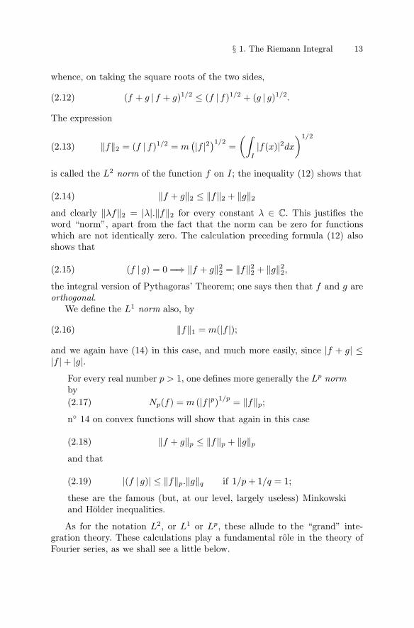
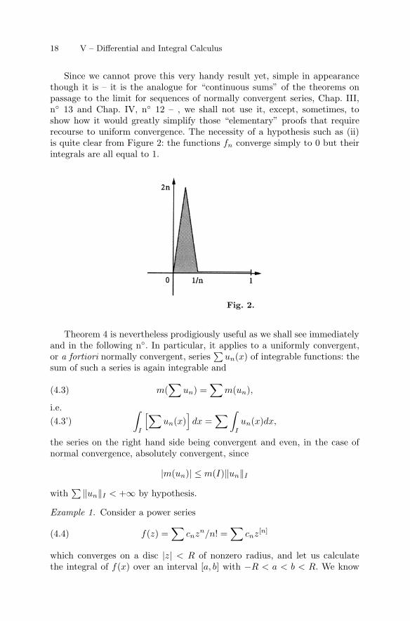
Since we cannot prove this very handy result yet, simple in appearancethough it is – it is the analogue for “continuous sums” of the theorems onpassage to the limit for sequences of normally convergent series, Chap. III,n◦ 13 and Chap. IV, n◦ 12 – , we shall not use it, except, sometimes, toshow how it would greatly simplify those “elementary” proofs that requirerecourse to uniform convergence. The necessity of a hypothesis such as (ii)is quite clear from Figure 2: the functions fn converge simply to 0 but theirintegrals are all equal to 1.
Fig. 2.
Theorem 4 is nevertheless prodigiously useful as we shall see immediatelyand in the following n◦. In particular, it applies to a uniformly convergent,or a fortiori normally convergent, series
∑un(x) of integrable functions: the
sum of such a series is again integrable and
m(∑
un) =∑
m(un),(4.3)
i.e. ∫I
[∑un(x)]dx =∑∫
I
un(x)dx,(4.3’)
the series on the right hand side being convergent and even, in the case ofnormal convergence, absolutely convergent, since
|m(un)| ≤ m(I)‖un‖I
with∑ ‖un‖I < +∞ by hypothesis.
Example 1. Consider a power series
f(z) =∑
cnzn/n! =∑
cnz[n](4.4)
which converges on a disc |z| < R of nonzero radius, and let us calculatethe integral of f(x) over an interval [a, b] with −R < a < b < R. We know
§ 1. The Riemann Integral 19
that the series converges normally on every disc |z| ≤ r < R, so on theinterval considered: we can therefore integrate term-by-term. But we alsoknow (Chap. II, n◦ 11) that∫ b
a
xndx =bn+1
n + 1− an+1
n + 1(4.5)
or, equivalently, that ∫ b
a
x[n]dx = b[n+1] − a[n+1].(4.5’)
Thus we find ∫ b
a
f(x)dx = F (b) − F (a)(4.6)
whereF (z) =
∑cnz[n+1] =
∑cn−1z
[n]
is the primitive power series of f in the sense of Chap. II, n◦ 19. Since wealso know that the function F is differentiable (in the complex sense on Cso a fortiori in the real sense on R) and that f is its derivative, (6) is just aparticular case of the “fundamental theorem” which we will establish later:
F ′ = f =⇒∫ b
a
f(x)dx = F (b) − F (a).
It was this kind of calculation that led Newton and Mercator to the series
log(1 + x) = x − x2/2 + x3/3 − . . .(4.7)
They knew (and we know: Chap. II, n◦ 11) that the left hand side is theintegral of the function t → 1/(1 + t) over the interval [0, x] and they wereaware of (5). The calculation is then obvious, particularly if one does notworry about Theorem 4 any more than they did. Conversely, if one firstknew the formula (7), one might deduce that the integral of the function1/(1 + x) between x = a and x = b is equal to log(1 + b) − log(1 + a), butthis assumes that a and b lie in the interval of convergence of (7): a directcalculation, in Chap. II, n◦ 11, has already provided the result free from thisrestriction. The reader may amuse himself by applying (6) in the same wayto the series representing ex, sin x, cos x, etc., since their primitive series canbe calculated immediately; one obtains the formulae∫ b
a
cos x.dx = sin b − sin a,
∫ b
a
sin x.dx = cos a − cos b,
∫ b
a
etxdx = (etb − eta)/t (t ∈ C, t �= 0),(4.8)
20 V – Differential and Integral Calculus
∫ b
a
dx/(1 + x2) = arctan b − arctan a,
etc., which confirm the “fundamental theorem”.
To conclude these trivialities on uniform limits we remark that the relation
lim fn = f =⇒ limm(fn) = m(f),(4.9)
valid in the framework of the uniform convergence, remains so under muchless restricted hypotheses.
If one replaces g by 1 in the Cauchy-Schwarz inequality one obtains therelation
|m(f)| ≤ m(I)1/2‖f‖2.(4.10)
From this one deduces that
lim ‖fn − f‖2 = 0 =⇒ limm(fn) = m(f);(4.11)
the same result holds for the Lp norms, p > 1, and for the norm ‖f‖1 since
|m(fn) − m(f)| ≤ ‖fn − f‖1
in this case. In other words, to obtain (9) it is enough to assume that thereexists a real number p ≥ 1 such that the integral of the function |fn(x)−f(x)|ptends to 0.
When lim ‖fn − f‖p = 0, one says that fn converges to f in mean oforder p (“in mean” for short if p = 1, “in quadratic mean” if p = 2). This isclearly the case if we have uniform convergence, but the converse is false sincethe value of an integral has no direct connection with that of the functionat a given point or even on the neighbourhood of a point. If for examplewe take on I = [0, 1] the functions fn(x) = n for 0 ≤ x ≤ 1/n2, = 0 ifnot, then we have m(fn) = 1/n and convergence to 0. What is essential toensure convergence in mean is that, for n large, the difference |fn(x)− f(x)|should not be > 10100 except on intervals of total length much smaller than10−100. All electricians know this, particularly in the case p = 2, since, forexample, to calculate the power dissipated by an electric current of variableintensity I(t) passing through a resistance during an interval of time [a, b],one integrates the function I(t)2 over it; “surges of current” have no influenceon the result if they are concentrated on sufficiently small intervals of time.
§ 1. The Riemann Integral 21
5 – Application to Fourier series and to power series
For a long time it was believed, and neophytes sometimes still believe, if theytrust to low level books, that integrals serve to calculate areas, volumes, cen-tres of gravity, magnetic flux, etc. This is not false, it was even positively truein the XVIIth century, but for ages they have served quite another purpose,namely: to do mathematics, in other words, to prove theorems. At the pointwhere we now are in expounding the theory, we still know almost nothing.Yet nevertheless . . .
Consider an absolutely convergent Fourier series of period 1, i.e. of theform
f(x) =∑
ane2πinx with∑
|an| < +∞,(5.1)
where one sums over all n ∈ Z and where the factor 2π has been introducedinto the exponents to simplify the formulae a little. Note in passing thatthe Euler relation eix = cos x + i. sin x allows us to write (1) in the moretraditional form
f(x) = a0 +∞∑
n=1
bn cos 2πnx + cn sin 2πnx
which is less convenient computationally.The first problem of the theory is to calculate the coefficients in (1) from f .
To this purpose we remark that, for any p, q ∈ Z and a ∈ R, we have7
∫ a+1
a
e2πipxe2πiqxdx =∫ a+1
a
e2πi(p−q)xdx ={
1 if p = q0 if p �= q
.(5.2)
If p = q we are integrating the constant function 1. If p �= q, we can putt = 2πi(p − q) and apply (4.8); we find the variation between x = a andx = a + 1 of the function etx/t; since t is a multiple of 2πi this function isof period 1, so takes the same values at a and a + 1 – there is no point incalculating them explicitly, except to increase the chance of error – so thatthe integral in question is zero. If, to simplify the notation, one puts
en(x) = e2πinx = exp(2πinx)(5.3)
and if one uses the notation
(f | g) =∫ a+1
a
f(x)g(x)dx = m(fg)(5.4)
of the end of n◦ 2 to denote the scalar product of two functions f and g ofperiod 1, then the preceding formulae can be written7 The integral over an interval [a, a+1] depends only on the integrand if the latter
is of period 1, as we saw at the end of n◦ 2.
22 V – Differential and Integral Calculus
(ep | eq) ={
1 if p = q.0 if p �= q.
(5.2’)
With this notation the series (1) can be written
f(x) =∑
anen(x).
For p ∈ Z given, let us consider the scalar product
(f | ep) = m(fep) = m(fe−p).
Since∑ |an| < +∞, and since the exponentials are all of modulus 1 because
the exponents are purely imaginary, the series
f(x)ep(x) =∑
anen(x)ep(x)
converges normally, so can be integrated term-by-term; in view of (2’) theonly term which yields a nonzero result in the integration is that for whichn = p, so finally we find the relation
ap = (f | ep) =∫ a+1
a
f(x)e−2πipxdx.(5.5)
This formula is the basis of the theory of Fourier series: one starts from agiven periodic function f(x), uses (5) to define the coefficients an and hopesthat the function f is represented by the series (1). This heavenly vision ofthe theory does not, alas, correspond to reality once one leaves the domain ofperiodic functions of class C1. To begin with, the series
∑an may well not
be absolutely convergent: the case of the square waves of Chap. III, n◦ 2.Let us now consider two absolutely convergent Fourier series
f(x) =∑
anen(x), g(x) =∑
bnen(x)
and calculate their scalar product. The multiplication theorem for absolutelyconvergent series shows that
f(x)g(x) =∑
apbqep(x)eq(x) =∑
apbqep−q(x)
on using the relations
ep(x)eq(x) = ep+q(x), en(x) = e−n(x) = en(−x).
The double series converges unconditionally and normally since by hypothesisthe series
∑an and
∑bn converge absolutely. We can then integrate term-
by-term over [0, 1], whence
(f | g) =∑
apbq (ep | eq);
§ 1. The Riemann Integral 23
the terms for which p �= q disappear and the Parseval-Bessel formula
(f | g) =∫ a+1
a
f(x)g(x)dx =∑
anbn(5.6)
remains. In particular, for any a ∈ R,
‖f‖22 = (f | f) =
∫ a+1
a
|f(x)|2dx =∑
|an|2.(5.7)
These proofs do not apply to the square wave series of Chap. III, n◦ 2and n◦ 11, but one can always examine what the results might mean in thiscase. To reduce to a Fourier series of period 1, one has to replace x by 2πxin the series cos x − cos 3x/3 + cos 5x/5 − . . ., i.e. to consider the series
f(x) = cos 2πx − cos(6πx)/3 + cos(10πx)/5 − . . .
= [e1(x) + e−1(x)] /2 − [e3(x)/3 + e−3(x)/3] /2 + . . .(5.8)
whose sum8, if one believes Fourier, is given by
f(x) = π/4 for |x| < 1/4, = −π/4 for 1/4 < |x| < 3/4,(5.9)
and by periodicity for the other values of x. If one accepts (9), the formula(5) with a = −1/4 here gives, up to a factor π/4 and using (4.8),
ap =∫ 1/4
−1/4
e−2πipxdx −∫ 3/4
1/4
e−2πipxdx =
=e−πip/2 − eπip/2
−2πip− e−3πip/2 − e−πip/2
−2πip=
=(eπip/2 − e−πip/2
)/2πip − e−πip
(eπip/2 − e−πip/2
)/2πip =
= [1 − (−1)p] sin(pπ/2)/πp,
zero if p is even, and equal to 2(−1)(p−1)/2/πp if p is odd; since we omitteda factor π/4, we finally have
ap = 0 (p even) or (−1)(p−1)/2/2p (p odd),
which agrees with (8). Thus here
∑|an|2 =
12(1 + 1/32 + 1/52 + . . .
)8 One might be tempted to write this series in the form
∑(−1)(n−1)/2en(x)/2n
where one sums over all odd n ∈ Z, but this unordered sum is no more convergentthan the harmonic series; only on grouping the symmetric terms do we obtain aconvergent Fourier series.
24 V – Differential and Integral Calculus
since each term is repeated twice. To apply (7), we again have to calculatethe integral, which is immediate since |f(x)|2 = π2/16 for every x. Hence theformula
1 + 1/32 + 1/52 + . . . = π2/8.(5.10)
Since one knows that
π2/6 =∑
1/n2 =∑
1/(2n)2 +∑
1/(2n − 1)2 = π2/24 +∑
1/(2n − 1)2,
it remains to observe that 1/6 − 1/24 = 1/8 to confirm that the result isindeed correct, even if the argument is unsupported for the moment; thisindicates that the hypothesis of absolute convergence in (5), (6) or (7), isprobably too restricting. And this is what the theory of Fourier series willshow.
Now let
f(z) =∑
anzn(5.11)
be a power series which converges on a disc |z| < R and therefore normallyon every disc |z| ≤ r < R. Consider the function f on the circle of radius r;again putting e2πit = e(t) with t real one finds
f [re(t)] =∑
anrnen(t),(5.12)
an absolutely convergent Fourier series having exponentials only of indexn ≥ 0. Therefore, by (5),∫ 1
0
f [re(t)]en(t)dt ={
anrn if n ≥ 0,0 if n < 0.
(5.13)
In particular, for n = 0,∫ 1
0
f(re2πit)dt = a0 = f(0),(5.14)
which means that the “mean value” of f on the circle |z| = r is equal to itsvalue at the centre of the circle, a curious property of the analytic functions.But there is better: since (13) allows us to calculate the coefficients an fromthe values of f on the circle of radius r it must be possible to calculate f(z),and not just f(0), in the same way.
Calculating formally for the moment, i.e. interchanging the∫
and∑
signs, applying (13) for a given r < R and substituting in (11) for a z suchthat |z| < r, we obtain
§ 1. The Riemann Integral 25
f(z) =∞∑0
anzn =∑
(z/r)nanrn =∞∑0
∫ 1
0
f [re(t)][z/re(t)]ndt =
=∫ 1
0
f [re(t)](∑
[z/re(t)]n)
dt =(5.15)
=∫ 1
0
re(t)re(t) − z
f [re(t)]dt for |z| < r,
since z and r do not depend on the variable of integration t. To justifythis calculation, i.e. Cauchy’s integral formula, which we shall write in an-other way below, it suffices to show that we are integrating a normally con-vergent series over [0, 1], see (4.3). The factor f [re(t)], bounded becauseit is a continuous function of t, is not important. The geometric series∑
(z/re(t))n must converge, which forces |z| < r. If this is the case, theformula |[z/re(t)]n| = (|z|/r)n = qn with q = |z|/r < 1 implies the normalconvergence of the series that we are integrating, qed.
Formula (15) shows that, on the disc |z| < r < R, we can calculate ffrom its values on the circumference |z| = r using an explicit formula of thesimplest kind. One normally states it in terms of re(t) = ζ, a function of twhose differential is
dζ = 2πire(t)dt;
then Cauchy’s formula is written, a la Leibniz, in the form
f(z) =1
2πi
∫f(ζ)dζ
ζ − z(5.16)
where one integrates along the circumference |ζ| = r and where |z| < r. Thisis, as we shall see later, a “curvilinear integral” (Chap. VIII, n◦s 2 and 4).
Conversely, any function f that is continuous for |z| ≤ r and satisfies (16)for |z| < r is a power series, i.e. is analytic in |z| < r : compute as in (15), butin the opposite order. This will later be used to prove that a uniform limit ofanalytic functions is analytic (Chap. VII, n◦ 19, where a more precise resultwill be found).
26 V – Differential and Integral Calculus
§ 2. Integrability Conditions
6 – The Borel-Lebesgue Theorem
As we have seen in Chap. II, n◦ 11, a very simple sufficient condition for theintegrability of a real function f is the existence for every r > 0 of a stepfunction ϕ such that
|f(x) − ϕ(x)| ≤ r for every x ∈ I;(6.1)
for then ϕ − r ≤ f ≤ ϕ + r and since the integrals of ϕ − r and ϕ + r areequal to within 2rm(I) the relation m∗(f) = m∗(f) follows.
The preceding property means that f is the uniform limit of step func-tions, so that the integrability of f would also follow from Theorem 4. Thefunctions possessing this property, i.e. the regulated functions of Chap. II,n◦ 11, have (Chap. III, n◦ 12) both left and right limits at every point of I.In this n◦ and the following, we shall show that this property characterisesthem, if I is compact.
The idea of the proof is very simple: the whole problem is to show that, forevery r > 0, one can decompose I into a finite number of subintervals Ik suchthat the given function f is constant to within r on each Ik. This conditionis clearly necessary if the condition (1) is to be satisfied; if, conversely, it issatisfied, and if one assumes, as one may, that the Ik are pairwise disjoint,one obtains (1) on taking ϕ to be equal to f(ξk) on Ik, where ξk is a pointchosen arbitrarily in Ik.
Now, given a function f that has right and left limits at every x ∈ I, it isvery easy to construct such intervals. Since, for every a ∈ I, the limits f(a+)and f(a−) exist, there is an open interval ]a, a + r′[ with left end-point aand an open interval ]a− r′′, a[ with right end-point a on which the functionis constant to within9 r. And of course it is constant to within r on theinterval [a, a]. If one then considers the open interval U(a) = ]a− r′′, a + r′[one obtains the following results: (i) each U(a) is the union of at most threeintervals on each of which f is constant to within r; (ii) U(a) contains a forevery a ∈ I. The theorem at which we aim would therefore be established ifwe could find a finite number of points ak such that
I ⊂⋃
U(ak)
since then I would be the union of its intersections with the U(ak), whichare composed of at most three intervals on which f is constant to within r.
9 If a is the right (resp. left) end-point of I, one may take any number > 0 forr′ (resp. r′′). If the function f is continuous, one can even find an open intervalwith centre a on which f is constant to within r, but this detail does not simplifythe following proof.
§ 2. Integrability Conditions 27
This kind of question certainly set mathematicians a-thinking from about1850 onwards, at least those who were concerned about the foundations ofanalysis and, in particular, about the properties of continuous functions.In their research on the “grand” integration theory, Emile Borel and HenriLebesgue came to isolate the crucial point which their predecessors (see The-orem 8 below) had more or less used, without appreciating the generality ofthe statement; it was later extended, like the Bolzano-Weierstrass theorem,to much more general spaces than R or C where the notion of a compact sethas meaning (see for example Dieudonne, Vol. I, Chap. III, n◦ 16).
Theorem 5 (Borel-Lebesgue). Let K be a compact subset of R (resp. C)and (Ui)i∈I a family of open sets in R (resp. C). Suppose that K is containedin the union of the Ui. Then there is a finite subset F of the set of indicesI such that K is contained in the union of the Ui, i ∈ F . This propertycharacterises the compact subsets of R (resp. C).
First we show that if K is bounded one can, for every r > 0, find a finitenumber of points xk of K such that K is contained in the union of the openballs B(xk, r). Since K is certainly contained in a compact interval or square,it is clear that one can find a finite number of open balls of radius r/2 whichcover K, i.e. whose union contains K. Let us choose an xk ∈ K in each ofthose of these balls Bk which actually intersect K. Since Bk is of radius r/2,so of diameter r, we have Bk ⊂ B(xk, r), so that the B(xk, r) cover K asdesired.
To prove the existence of F , it thus suffices to show that there exists anumber r > 0 possessing the following property:
(∗) for every x ∈ K the open ball B(x, r) is contained in one ofthe Ui.
If this is so, then it is enough to choose a Ui containing B(xk, r) for each kto obtain the first assertion of the theorem.
Suppose (*) is false. For every n ∈ N there then must exist an x(n) ∈ Ksuch that the ball B(x(n), 1/n) is not contained in any of the Ui. By BW,since K is compact, one can extract from the sequence x(n) a subsequencex(pn) which converges to an a ∈ K (Chap. III, n◦ 9). Since one of the Ui
contains a, and is open, it contains a ball B(a, r) of radius r > 0. For n largeone has both |a − x(pn)| < r/2 and 1/pn < r/2. It follows that the ballB(x(pn), 1/pn) is contained in B(a, r) and a fortiori in Ui, a contradiction.
It remains to show that the compact sets are the only ones to have theBL property. In the first place, a set K which has it is bounded; indeed, Kis covered by the family of the open balls B(x, 1), x ∈ K, since any ballcontains its centre; there is then a finite number of xk ∈ K such that theB(xk, 1) cover K, whence this property.
On the other hand, K is closed, i.e. contains every adherent point a. Letus assume the opposite and let a /∈ K be an adherent point of K. For every
28 V – Differential and Integral Calculus
n ∈ N, denote by Un the set of x ∈ R (or C) such that d(x, a) > 1/n, i.e.the exterior of the ball B(a, 1/n). The Un are open and cover K: for everyx ∈ K one has d(x, a) > 0 since a /∈ K, whence, for n large, d(x, a) > 1/n,i.e. x ∈ Un. If then K has the Borel-Lebesgue property one can cover it bya finite number of sets Un; but since these form an increasing sequence thismeans that K ⊂ Un for n large, in other words that the closed ball B(a, 1/n)complementing Un in R (or C) does not meet K. Contradiction, since a isadherent to K, qed.
By a curious coincidence, the essential tool in this proof is the Bolzano-Weierstrass theorem, which, as we know (Chap. III, n◦ 9), characterises thecompact subsets of R or C. We may therefore wonder whether, conversely, itis possible to deduce BW from BL, which would allow the reader to add BLto the list of the statements equivalent to the axiom (IV) of R (Chap. III, endof n◦ 10). For a proof, see Dieudonne, Elements d’analyse, Vol. I, Chap. III,n◦ 16.
Corollary 1. Let (Ki)i∈I be a family of nonempty compact sets in R or C.Suppose that the intersection of the Ki is empty. Then there is a finite subsetF of I such that the intersection of the Ki, i ∈ F , is empty.
We choose any index j and replace each Ki by Ki ∩ Kj . If one of theseintersections is empty, the corollary is proved. So assume they are nonempty.This is equivalent to assuming that all the Ki are contained in the samecompact set K, namely Kj .
Let Ui be the complement of Ki in R (or C). It is open since Ki is closed.The union of the Ui is the complement of the intersection of the Ki. If thisis itself empty then the Ui cover R (or C) and thus K. By BL, there existsa finite set F ⊂ I such that the Ui, i ∈ F , cover K. The complement of theunion of these Ui is the intersection of the Ki, i ∈ F . This cannot intersectK; and since it is contained in K it must be empty, qed.
If we putKF =
⋂i∈F
Ki
for every finite subset F of I we can reformulate the preceding corollaryas follows: the Ki have a point in common if and only if KF is nonemptyirrespective of F . The case where the Ki are intervals in R has already beentreated in Chap. III, n◦ 9.
The reader will perhaps wonder why it is necessary to assume the Ui openin the BL theorem. A trivial counterexample: cover K by the closed sets {x},x ∈ K; if K is infinite it is clearly impossible to cover it by a finite numberof such sets. One might prefer a less crude counterexample. Take K = [−1, 1]and cover it by the intervals ]1/2, 1], ]1/3, 1/2], . . . and [−2, 0]. Every x > 0 inK belongs to one and only one interval ]1/n, 1/(n+1)], and every x < 0 to theinterval [−2, 0]; the obstacle would fall if one had chosen [−2, r] with an r > 0.
§ 2. Integrability Conditions 29
Another important consequence of BL is the local character of uniformconvergence on a compact set:
Corollary 2. Let X be a subset of C and (fn) a sequence of scalar functionsdefined on X, converging simply to a limit f . Assume that, for every a ∈ X,there exists a ball B(a) of centre a such that the fn converge to f uniformlyon B(a) ∩ X. Then the fn converge uniformly on every compact K ⊂ X(“compact convergence” on X).
We may assume the B(a) open. By BL, one can cover K by a finitenumber of balls B(ai). For r > 0 given, the assertion
|fn(x) − f(x)| < r for every x ∈ B(ai) ∩ K(6.2)
is, for each i, true for n large. Since, for r given, these relations are finitein number, they are thus simultaneously true for n large (Chap. II, n◦ 3),and since the union of the B(ai) ∩ K is K, it follows that, for n large, theinequality (2) is true for all the x ∈ K simultaneously, qed.
Corollary 2 is particularly useful in the theory of analytic functions; X isthen an open subset of C and it is often easy to show that, for every a ∈ X,the convergence of the fn is uniform on a sufficiently small disc with centrea, whence compact convergence on X.
7 – Integrability of regulated or continuous functions
The arguments which led us to formulate the BL theorem at the beginningof the preceding n◦ lead to the following result:
Theorem 6. Let f be a scalar function defined on an interval I of R. Thetwo following properties are equivalent: (i) f has left and right limits at everypoint of I; (ii) there is a sequence of step functions on I which converges tof uniformly on every compact subset of I. The function f is then continuouson the complement of a countable subset of I.
The implication (ii) =⇒ (i) was established from Cauchy’s criterion inChap. III, n◦ 12 (Corollary of Theorem 16). The implication (i) =⇒ (ii)is obtained, when I is compact, by observing, as at the beginning of thepreceding n◦, that for every r > 0, there exists for every x ∈ I an openinterval U(x) =]x− r′′, x + r′[ such that f is constant to within r on each ofthe three intervals ]x − r′′, x[, [x, x] and ]x, x + r′[; it remains only to applyBL to the U(x) to obtain a finite number of intervals covering I and on eachof which f is constant to within r; this argument also shows that f is boundedon every compact K ⊂ I.
In the case of a not necessarily compact interval I one clearly has to workon an arbitrary compact interval K contained in I. One sees then that thefollowing two properties are equivalent for a scalar function f defined on I:
30 V – Differential and Integral Calculus
(i) f has right and left limits at every point of I, in other words, by definition,is regulated on I;
(ii) for every compact interval K ⊂ I there exists a sequence of step functionson K which converges to f uniformly on K.
One can then find a sequence (ϕn) of step functions on I (i.e. such that onecan partition I into a finite number of intervals on each of which the functionis constant) which, for every compact K ⊂ I, converges to f uniformly on K:choose an increasing sequence of compact intervals Kn with union I and, foreach n, a step function ϕn on Kn satisfying |f(x) − ϕn(x)| < 1/n for everyx ∈ Kn, and then define ϕn on all of I by agreeing that ϕn(x) = 0 for everyx ∈ I − Kn. Again limϕn(x) = f(x) for every x ∈ I because x ∈ Kp for plarge, whence |f(x) − ϕn(x)| < 1/n for every x ∈ Kp and every n ≥ p sincethen Kp ⊂ Kn.
It remains to prove the continuity of f . For every n, let Dn be the finiteset of the points of I where ϕn is discontinuous. The union D of the Dn iscountable (Chap. I) and the ϕn, as functions defined on I, are all continuousat every x ∈ I − D. Similarly10 for f , qed.
Note that the theorem applies to monotone functions in particular.
Corollary. Every bounded and regulated function f on a bounded intervalI = (a, b) is integrable on I, and∫ b
a
f(x)dx = limu→a+,v→b−
∫ v
u
f(x)dx.(7.1)
Choose an r > 0 and a compact interval K = [u, v] contained in I and suchthat m(I)−m(K) < r. By Theorem 6 the function f is integrable on K. Theremust therefore exist on K a step function ϕ such that mK(|f−ϕ|) < r, wheremK is the integral over K. We define a step function ϕ′ on I by requiring itto be equal to ϕ on K and zero off K. Since |f(x)−ϕ′(x)| ≤ ‖f‖I off K, wesee, separating the contributions over K and I − K, that∫
I
|f(x) − ϕ′(x)| dx ≤ r + [m(I) − m(K)] ‖f‖I ≤ (1 + ‖f‖I) r,
whence f is integrable on I. Relation (1) follows on remarking that the dif-ference between the integrals over I and [u, v] is the sum of the integrals over]a, u] and [v, b[, intervals whose lengths tend to 0, qed.
We will rediscover this in § 7 a propos the integration of not necessarilybounded functions over arbitrary intervals. Up to then integrals over a com-pact interval will almost always be sufficient for our needs, but it is goodto know that in spite of its unorthodox behaviour on a neighbourhood of 0,the function sin(1/x) is integrable over ]0, 1] in the sense of n◦ 2, the mostelementary that there is.10 To avoid all confusion, recall that we are dealing with the continuity of f as a
function on I and not only on I − D. See n◦ 5 of Chap. III again.
§ 2. Integrability Conditions 31
The arguments showing that (i) =⇒ (ii) also serve to establish the fol-lowing result, already mentioned in n◦ 3:
Theorem 7. The integral of a regulated (resp. continuous) positive functionf is zero if and only if the set D = {f(x) �= 0} is countable (resp. empty).
The condition is sufficient. For consider a step function ϕ ≤ f . One canhave ϕ(x) > 0 only if x ∈ D. Since the set of points of a nonsingletoninterval is uncountable (Chap. I), the function ϕ is necessarily negative onall the intervals of nonzero length where it is constant. Thus m(ϕ) ≤ 0 and,since m(f) is the upper bound of these m(ϕ), we also have m(f) ≤ 0, whencem(f) = 0 since f is positive.
To show that it is necessary, we assume first that I is compact and con-struct a sequence (ϕn) of step functions on I such that ‖f − ϕn‖I ≤ 1/n.Replacing ϕn by ϕn − 1/n, we may assume that ‖f − ϕn‖I ≤ (1 + m(I))/nand ϕn ≤ f . Since f ≥ 0 one can even assume ϕn ≥ 0 (replace them bythe ϕ+
n ). Then m(ϕn) = 0 since m(f) = 0. Each ϕn is then zero outsidea finite set Dn. The union D of the Dn is countable (Chap. I) and sincef(x) = limϕn(x) for every x ∈ I it is clear that f(x) = 0 for every x /∈ D.
If now I is not compact it is the union of a sequence of compact Kn. Theintegral of f over each Kn is clearly zero; the D∩Kn are therefore countable,so D =
⋃D ∩ Kn (Ch. I) is too.
If f is continuous then D is open and so, if not empty, must contain aninterval of length > 0, which would have to be countable like D, contrary toCantor’s most famous theorem, qed.
A corollary of Theorem 7 is that if two regulated functions f and g areequal outside a countable set D then m(f) = m(g). For the function |f −g| isagain regulated11 and it is positive; Theorem 7 then shows that m(|f−g|) = 0,whence m(f) = m(g).
One might be tempted to believe that conversely, if one modifies the valuesof a regulated function f on a countable set D of points, one will again findan integrable or even regulated function. False: the constant function equalto 1 is as regulated as it is possible to be, but if you change it to have thevalue 0 at rational points you will obtain the Dirichlet function which isneither regulated nor Riemann integrable.
8 – Uniform continuity and its consequences
The principal interest of Theorem 6 is to show that every regulated functionis integrable. In particular this is the case for continuous functions. The proof11 Obvious. Note, in this circle of ideas, that if f is regulated and if g is continuous
then the composite function g ◦ f is again regulated, since if x tends to c+ orc−, then f(x) tends to f(c+) or f(c−), so that g[f(x)] tends to a limit, namelyg[f(c+)] or g[f(c−)], qed. This result may not follow if g is only regulated.
32 V – Differential and Integral Calculus
of the implication (i) =⇒ (ii) of Theorem 6 allows us to isolate an importantproperty that they have, namely uniform continuity.
Consider, generally, a scalar function f defined and continuous on a subsetX of R or C. For every r > 0 and every x ∈ X there exists a number r′ > 0such that, for y ∈ X,
d(x, y) ≤ r′ =⇒ d[f(x), f(y)] ≤ r.(8.1)
The number r′ depends a priori on the choice of r and of x. One says thatf is uniformly continuous on X if, for every r > 0, you can choose the samer′ > 0 for all x ∈ X, so that
{(x ∈ X) & (y ∈ X) & (d(x, y) ≤ r′)} =⇒ d[f(x), f(y)] ≤ r.(8.2)
Suppose for example that X = R and let us put y = x − h. Then (2) meansthat
|h| ≤ r′ =⇒ |f(x − h) − f(x)| ≤ r for every x ∈ R.(8.3)
Now let us introduce the translated functions
fh(x) = f(x − h)(8.4)
of f whose graphs are derived from the graph of f by horizontal translations.This said, the fact that d[fh(x), f(x)] ≤ r for every x means simply, in thenotation of Chap. III, n◦ 7, that
dR(f, fh) = ‖f − fh‖R ≤ r.(8.5)
The existence, for every r > 0, of an r′ > 0 satisfying (3) thus means that ash tends to 0 the function fh(x) converges to f(x) uniformly on R. One wouldlike to formulate uniform continuity on an arbitrary set X in a similar way,but in this case the function fh(x) is defined only on the set �= X formed fromX by the horizontal translation of amplitude h, and convergence, uniform ornot, no longer has a meaning.
Uniform continuity is very far from being a universal property of contin-uous functions. If you take the function f(x) = ex on R for example, whenfh(x) = e−hf(x), it is clear that, as h tends to 0, fh converges simply to f –this is continuity –, but for a given h the difference |f(x)−fh(x)| = |e−h−1|ex
is not even bounded on R, which rules out uniform convergence: in this case‖f − fh‖R = +∞ for any h �= 0.
We always have:
Theorem 8 (Heine12). Every scalar function defined and continuous on acompact set K ⊂ C is uniformly continuous on K.
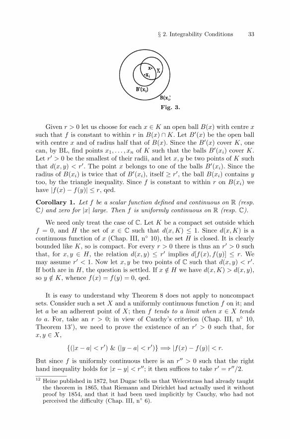
§ 2. Integrability Conditions 33
Fig. 3.
Given r > 0 let us choose for each x ∈ K an open ball B(x) with centre xsuch that f is constant to within r in B(x) ∩ K. Let B′(x) be the open ballwith centre x and of radius half that of B(x). Since the B′(x) cover K, onecan, by BL, find points x1, . . . , xn of K such that the balls B′(xi) cover K.Let r′ > 0 be the smallest of their radii, and let x, y be two points of K suchthat d(x, y) < r′. The point x belongs to one of the balls B′(xi). Since theradius of B(xi) is twice that of B′(xi), itself ≥ r′, the ball B(xi) contains ytoo, by the triangle inequality. Since f is constant to within r on B(xi) wehave |f(x) − f(y)| ≤ r, qed.
Corollary 1. Let f be a scalar function defined and continuous on R (resp.C) and zero for |x| large. Then f is uniformly continuous on R (resp. C).
We need only treat the case of C. Let K be a compact set outside whichf = 0, and H the set of x ∈ C such that d(x,K) ≤ 1. Since d(x,K) is acontinuous function of x (Chap. III, n◦ 10), the set H is closed. It is clearlybounded like K, so is compact. For every r > 0 there is thus an r′ > 0 suchthat, for x, y ∈ H, the relation d(x, y) ≤ r′ implies d[f(x), f(y)] ≤ r. Wemay assume r′ < 1. Now let x, y be two points of C such that d(x, y) < r′.If both are in H, the question is settled. If x /∈ H we have d(x,K) > d(x, y),so y /∈ K, whence f(x) = f(y) = 0, qed.
It is easy to understand why Theorem 8 does not apply to noncompactsets. Consider such a set X and a uniformly continuous function f on it; andlet a be an adherent point of X; then f tends to a limit when x ∈ X tendsto a. For, take an r > 0; in view of Cauchy’s criterion (Chap. III, n◦ 10,Theorem 13’), we need to prove the existence of an r′ > 0 such that, forx, y ∈ X,
{(|x − a| < r′) & (|y − a| < r′)} =⇒ |f(x) − f(y)| < r.
But since f is uniformly continuous there is an r′′ > 0 such that the righthand inequality holds for |x − y| < r′′; it then suffices to take r′ = r′′/2.12 Heine published in 1872, but Dugac tells us that Weierstrass had already taught
the theorem in 1865, that Riemann and Dirichlet had actually used it withoutproof by 1854, and that it had been used implicitly by Cauchy, who had notperceived the difficulty (Chap. III, n◦ 6).
34 V – Differential and Integral Calculus
In these circumstances it is natural to define a function F on the closure13
X of X by puttingF (a) = lim
x→a,x∈Xf(x)
for every a ∈ X; we have F (a) = f(a) if a ∈ X. Let us show that the functionF is continuous on X. For every r > 0 we choose an r′ > 0 such that, forx, y ∈ X,
|x − y| < r′ =⇒ |f(x) − f(y)| < r
and consider two points a, b of X such that |a− b| < r′ (strict inequality). Ifx, y ∈ X are sufficiently close to a and b respectively, we again have |x−y| < r′
and so |f(x)− f(y)| < r; since f(x) and f(y) tend to F (a) and F (b), we findin the limit that |F (a) − F (b)| ≤ r, whence the result.
This shows that the notion of uniform convergence in reality concerns onlycontinuous functions on a closed set, or, equivalently, which can be extendedto a closed set while remaining continuous (and even uniformly continuous).In particular:
Corollary 2. Let f be a function defined and continuous on a bounded setX ⊂ C. The following two properties are equivalent: (i) f is uniformly con-tinuous on X; (ii) f is the restriction to X of a continuous function on thecompact set X.
We have just seen that (i) implies (ii). The converse implication followsfrom Theorem 8 since X is compact.
If, for example, X =]0, 1], the function f(x) = sin(1/x) manifestly has nolimit when x tends to 0; this does not prevent it from being integrable sinceit is continuous and bounded (Corollary to Theorem 6), but does preventit from being uniformly continuous on X. To verify this by a subtle use ofinequalities is a gymnastic exercise in the Weierstrass tradition; Corollary 2makes this quite unnecessary: there are enough serious occasions for dealingwith inequalities that one prefers not to when one can obtain the result free.One might, otherwise, advise the amateurs to examine such functions as
sin(sin(1/x)), sin(exp(sin(1/x))), etc.
“by hand”.Corollary 2 allows us to answer an approximation problem: can one ap-
proximate a given continuous function on X by polynomials uniformly onX? We shall show in n◦ 28 that this is so if X is a compact interval in R (orC so long as one uses polynomials in x and y, and not in z = x + iy). But ifX is bounded without being compact?
Let p be a polynomial satisfying |f(x)− p(x)| ≤ r for every x ∈ X. Sincethe function p is continuous on R and so on the compact closure of X, it13 Recall that this is the set of points that one can approximate by the x ∈ X, or,
again, the smallest closed set containing X.
§ 2. Integrability Conditions 35
is uniformly continuous on X. There is therefore an r′ > 0 such that, forx, y ∈ X, the relation |x− y| < r′ implies |p(x)− p(y)| < r and consequently|f(x) − f(y)| < 3r. In other words, if f is the uniform limit of polynomi-als (or, more generally, of uniformly continuous functions on X), then f isuniformly continuous on X. Conversely, f may then be extended to a con-tinuous function on the compact set X and Weierstrass’ theorem providesthe desired approximation on X, so a fortiori on X. The question thus lacksinterest: when the answer is affirmative it results from Weierstrass’ theoremfor a compact set. On the other hand we have shown in Chap. III, n◦ 5 thatif X is an unbounded interval in R then the only uniform limits of polyno-mials in X are the polynomials themselves. Moral: do not try to “improve”Weierstrass’ theorem . . .
Another consequence of Heine’s theorem is the possibility of defining theintegral of a continuous function f over a compact interval I by means of thestandard Riemann sums.
One can, for example, like Cauchy, consider arbitrary subdivisions of Iand the sums
∑f(xk)(xk+1 − xk) which irresistibly evoke Leibniz’ notation∫
f(x)dx (the evocation, as concerns Cauchy, would rather go in the inversesense . . .) or even the more general sums
∑f(ξk)(xk+1 −xk) with the points
ξk chosen arbitrarily in the closed intervals14 [xk, xk+1]. If, on each of theseintervals, the function is constant to within r, the function f is everywhereequal to within r to the step function equal to f(ξk) on [xk, xk+1[, so that theintegral of f is equal to the sum considered to within m(I)r. But since f isuniformly continuous this condition will be satisfied so long as |xk+1−xk| < r′
for a suitably chosen r′ > 0. In other words:
Corollary 3. Let f be a scalar function defined and continuous on a compactinterval I. For every r > 0 there exists an r′ > 0 such that∣∣∣∣
∫I
f(x)dx −∑
f(ξk)(xk+1 − xk)∣∣∣∣ < r(8.6)
for any points ξk ∈ [xk, xk+1] so long as the subdivision (xk) of I satisfies|xk+1 − xk| < r′ for every k.
For example one can decompose I into n equal intervals I1, . . . , In andchoose a ξk ∈ Ik at random for each k. The corresponding Riemann sum isjust
m(I)f(ξ1) + . . . + f(ξn)
n.
It tends to the integral of f as n increases indefinitely. This remark explainswhy the ratio m(f)/m(I) between the integral of f and the measure of I iscalled the mean value of the function f on I .14 For a general regulated function we have seen above that the ξk must be interior
to the intervals of the subdivision because the function f may be discontinuousat the points xk.
36 V – Differential and Integral Calculus
9 – Differentiation and integration under the∫
sign
We shall continue to explain various important consequences of uniform conti-nuity. We have established them not only in R, but also in C, i.e. for functionsof two real variables.
Consider a function f(x, y) defined and continuous on a rectangle K × Jin C, where K and J are intervals in R, and K is assumed compact as itsname suggests. We can integrate f(x, y) with respect to x for given y, andmore generally consider the function
ϕ(y) =∫
K
f(x, y)µ(x)dx(9.1)
where µ is an arbitrary integrable function on K (if not a Radon measure. . .).
Theorem 9. Let K be a compact interval, J an arbitrary interval of R, andlet f(x, y) be a continuous function on K × J . Then
(i) the function (1) is continuous in J ;(ii) if f has a continuous partial derivative D2f(x, y) on K × J then ϕ is of
class C1 on J and
ϕ′(y) =∫
K
D2f(x, y)µ(x)dx.(9.2)
Continuity and differentiability at a point y being local properties we canreplace J in what follows by a compact interval H ⊂ J containing all pointsof J sufficiently close to y.
Generally, put µ(f) =∫
f(x)µ(x)dx for every function f continuous on K,whence, omitting the K under the
∫sign,
|µ(f)| ≤∫
|f(x)|.|µ(x)|dx ≤ M(µ)‖f‖K
where M(µ) =∫ |µ(x)|dx. Then ϕ(y) = µ(fy) where fy(x) = f(x, y).
Since f is continuous and so uniformly continuous on the compact setK × H, one can associate with every r > 0 an r′ > 0 such that, on K × H,
(|x′ − x′′| < r′) & (|y′ − y′′| < r′) =⇒ |f(x′, y′) − f(x′′, y′′)| < r.(9.3)
For |y′−y′′| < r′ one then has |f(x, y′)−f(x, y′′)| < r, i.e. |fy′(x) − fy′′(x)| < r,for every x ∈ K; consequently,
|y′ − y′′| < r′ =⇒ ‖fy′ − fy′′‖K ≤ r.(9.4)
This means that, as y′′ tends to y′, the function fy′′ converges to fy′ uniformlyon K. The continuity of ϕ follows from this since
§ 2. Integrability Conditions 37
|ϕ(y′) − ϕ(y′′)| = |µ(fy′) − µ(fy′′)| ≤ M(µ)‖fy′ − fy′′‖K ≤ M(µ)r
for |y′ − y′′| < r′.As to differentiability, we put D2f = g, gy(x) = g(x, y) and denote the
right hand side of (2) by ψ(y) = µ(gy), a continuous function of y by (i)applied to g. Then
ϕ(y + h) − ϕ(y)h
− ψ(y) =µ(fy+h) − µ(fy)
h− µ(gy) =(9.5)
= µ [(fy+h − fy)/h − gy]
by the linearity of f → µ(f). To show that the left hand side tends to 0 withh, it suffices to show that, as h tends to 0, the function of x to be integrated(in the third term) tends to 0 uniformly on K for y given.
Now we proved in Chap. III, n◦ 16 (Corollary 4 of the Mean Value The-orem) that for every differentiable function p on a compact interval [a, b], wehave
|p(b) − p(a) − p′(c)(b − a)| ≤ |b − a|. sup |p′(x) − p′(c)|for every c ∈ [a, b], the sup being taken over the x ∈ [a, b]. We apply thisresult to the function y → f(x, y) for x given; we obtain
|f(x, y + h) − f(x, y) − D2f(x, y)h| ≤ |h|. sup |D2f(x, y + k) − D2f(x, y)|,the sup being taken over the k lying between 0 and h. The function D2fbeing continuous and so uniformly continuous on the compact set K × H,there exists for every r > 0 an r′ > 0 such that
|k| ≤ r′ =⇒ |D2f(x, y + k) − D2f(x, y)| ≤ r
for any x ∈ K and y ∈ H. We deduce that
|h| ≤ r′ =⇒ |f(x, y + h) − f(x, y) − D2f(x, y)h| ≤ r|h|,i.e. that
|h| ≤ r′ =⇒ |fy+h(x) − fy(x) − hgy(x)| ≤ r|h|,for any x ∈ K. On taking the sup for x ∈ K and dividing by |h|, we deducethat
|h| ≤ r′ =⇒ ‖(fy+h − fy)/h − gy‖K ≤ r,(9.6)
which proves uniform convergence as announced, or, if one prefers, showsthat the left hand side of (5) is ≤ M(µ)r, qed.
Let now K and H be two compact intervals, µ and ν two integrablefunctions on K and H and f a continuous function in K × H. We can thenconsider the iterated integral which we denote by
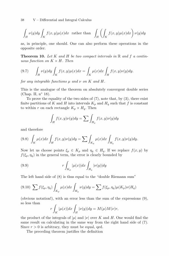
38 V – Differential and Integral Calculus
∫H
ν(y)dy
∫K
f(x, y)µ(x)dx rather than∫
H
(∫K
f(x, y)µ(x)dx
)ν(y)dy
as, in principle, one should. One can also perform these operations in theopposite order.
Theorem 10. Let K and H be two compact intervals in R and f a contin-uous function on K × H. Then∫
H
ν(y)dy
∫K
f(x, y)µ(x)dx =∫
K
µ(x)dx
∫H
f(x, y)ν(y)dy.(9.7)
for any integrable functions µ and ν on K and H.
This is the analogue of the theorem on absolutely convergent double series(Chap. II, n◦ 18).
To prove the equality of the two sides of (7), note that, by (3), there existfinite partitions of K and H into intervals Kp and Hq such that f is constantto within r on each rectangle Kp × Hq. Then∫
H
f(x, y)ν(y)dy =∑∫
Hq
f(x, y)ν(y)dy
and therefore∫K
µ(x)dx
∫H
f(x, y)ν(y)dy =∑∫
Kp
µ(x)dx
∫Hq
f(x, y)ν(y)dy.(9.8)
Now let us choose points ξp ∈ Kp and ηq ∈ Hq. If we replace f(x, y) byf(ξp, ηq) in the general term, the error is clearly bounded by
r
∫Kp
|µ(x)|dx
∫Hq
|ν(y)|dy(9.9)
The left hand side of (8) is thus equal to the “double Riemann sum”
∑f(ξp, ηq)
∫Kp
µ(x)dx
∫Hq
ν(y)dy =∑
f(ξp, ηq)µ(Kp)ν(Hq)(9.10)
(obvious notation!), with an error less than the sum of the expressions (9),so less than
r
∫K
|µ(x)|dx
∫H
|ν(y)|dy = M(µ)M(ν)r,
the product of the integrals of |µ| and |ν| over K and H. One would find thesame result on calculating in the same way from the right hand side of (7).Since r > 0 is arbitrary, they must be equal, qed.
The preceding theorem justifies the definition
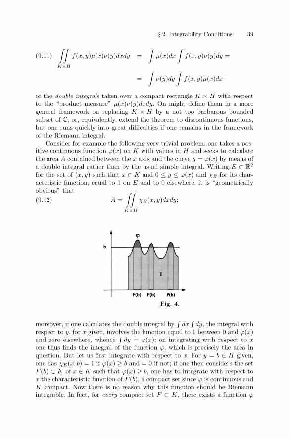
§ 2. Integrability Conditions 39
∫∫K×H
f(x, y)µ(x)ν(y)dxdy =∫
µ(x)dx
∫f(x, y)ν(y)dy =(9.11)
=∫
ν(y)dy
∫f(x, y)µ(x)dx
of the double integrals taken over a compact rectangle K × H with respectto the “product measure” µ(x)ν(y)dxdy. On might define them in a moregeneral framework on replacing K × H by a not too barbarous boundedsubset of C, or, equivalently, extend the theorem to discontinuous functions,but one runs quickly into great difficulties if one remains in the frameworkof the Riemann integral.
Consider for example the following very trivial problem: one takes a pos-itive continuous function ϕ(x) on K with values in H and seeks to calculatethe area A contained between the x axis and the curve y = ϕ(x) by means ofa double integral rather than by the usual simple integral. Writing E ⊂ R2
for the set of (x, y) such that x ∈ K and 0 ≤ y ≤ ϕ(x) and χE for its char-acteristic function, equal to 1 on E and to 0 elsewhere, it is “geometricallyobvious” that
A =∫∫K×H
χE(x, y)dxdy;(9.12)
Fig. 4.
moreover, if one calculates the double integral by∫
dx∫
dy, the integral withrespect to y, for x given, involves the function equal to 1 between 0 and ϕ(x)and zero elsewhere, whence
∫dy = ϕ(x); on integrating with respect to x
one thus finds the integral of the function ϕ, which is precisely the area inquestion. But let us first integrate with respect to x. For y = b ∈ H given,one has χE(x, b) = 1 if ϕ(x) ≥ b and = 0 if not; if one then considers the setF (b) ⊂ K of x ∈ K such that ϕ(x) ≥ b, one has to integrate with respect tox the characteristic function of F (b), a compact set since ϕ is continuous andK compact. Now there is no reason why this function should be Riemannintegrable. In fact, for every compact set F ⊂ K, there exists a function ϕ
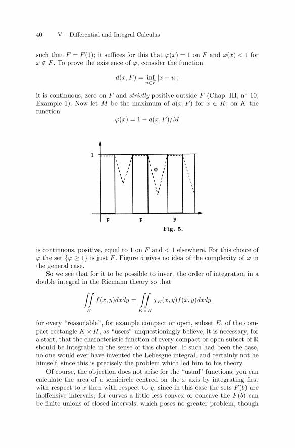
40 V – Differential and Integral Calculus
such that F = F (1); it suffices for this that ϕ(x) = 1 on F and ϕ(x) < 1 forx /∈ F . To prove the existence of ϕ, consider the function
d(x, F ) = infu∈F
|x − u|;
it is continuous, zero on F and strictly positive outside F (Chap. III, n◦ 10,Example 1). Now let M be the maximum of d(x, F ) for x ∈ K; on K thefunction
ϕ(x) = 1 − d(x, F )/M
Fig. 5.
is continuous, positive, equal to 1 on F and < 1 elsewhere. For this choice ofϕ the set {ϕ ≥ 1} is just F . Figure 5 gives no idea of the complexity of ϕ inthe general case.
So we see that for it to be possible to invert the order of integration in adouble integral in the Riemann theory so that∫∫
E
f(x, y)dxdy =∫∫K×H
χE(x, y)f(x, y)dxdy
for every “reasonable”, for example compact or open, subset E, of the com-pact rectangle K ×H, as “users” unquestioningly believe, it is necessary, fora start, that the characteristic function of every compact or open subset of Rshould be integrable in the sense of this chapter. If such had been the case,no one would ever have invented the Lebesgue integral, and certainly not hehimself, since this is precisely the problem which led him to his theory.
Of course, the objection does not arise for the “usual” functions: you cancalculate the area of a semicircle centred on the x axis by integrating firstwith respect to x then with respect to y, since in this case the sets F (b) areinoffensive intervals; for curves a little less convex or concave the F (b) canbe finite unions of closed intervals, which poses no greater problem, though
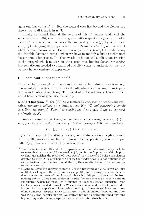
§ 2. Integrability Conditions 41
again one has to justify it. But the general case lies beyond the elementarytheory; we shall treat it in n◦ 33.
Finally we remark that all the results of this n◦ remain valid, with thesame proofs (n◦ 30), when one integrates with respect to a general “Radonmeasure” i.e. when one replaces the integral f → m(f) by a functionf → µ(f) satisfying the properties of linearity and continuity of Theorem 1which, alone, feature in all that we have just done (except for calculatingthe “double Riemann sums”, when we have to modify a little to eliminatediscontinuous functions). In other words, it is not the explicit constructionof the integral which matters in these problems, but its formal properties.Mathematicians needed two hundred and fifty years to understand this, butwe now have a century of experience.
10 – Semicontinuous functions15
To know that the regulated functions are integrable is almost always enoughin elementary practice, but it is not difficult, where we now are, to anticipatethe “grand” integration theory. The essential tool is a famous theorem whichwould have been of great use to Cauchy:
Dini’s Theorem. 16 Let (fn) be a monotone sequence of continuous real-valued functions defined on a compact set K ⊂ C and converging simplyto a limit function f . Then f is continuous if and only if the fn convergeuniformly on K.
We can assume that the given sequence is increasing, whence f(x) =sup fn(x) for every x ∈ K. For every r > 0 and every a ∈ K, we then have
f(a) ≥ fn(a) > f(a) − r for n large.
If f is continuous, this relation is, for n given, again true on a neighbourhoodof a. By BL, we can then find a finite number of points ap ∈ K and openballs B(ap) covering K such that each relation15 The contents of n◦ 10 and 11, preparation for the Lebesgue theory, will be
repeated in a more general framework in § 9, and in the Appendix to this chapter;we shall use neither the results of these two n◦ nor those of § 9 before the chapterdevoted to them. Our aim here is to show the reader that it is not difficult to gorather further than the traditional theory, the essential being to know how fartoo far not to go . . .
16 Having followed the analysis courses of Joseph Bertrand and J.A. Serret at Parisin 1866, as Dugac tells us in his thesis, p. 106, and having conceived seriousdoubts as to the rigour of their ideas, doubts which his youth dissuaded him frommaking public, Ulisse Dini, professor at Pisa (where there is an “Ecole normalesuperieure” which has produced a number of excellent Italian scientists), readthe Germans, educated himself on Weierstrass’ course, and, in 1878, published inItalian the first exposition of analysis according to Weierstrass’ ideas and thoseof his numerous disciples, followed in 1880 by a book on Fourier series. His bookwas widely read because neither Weierstrass nor his disciples published anythingbeyond duplicated manuscript courses of very limited distribution.
42 V – Differential and Integral Calculus
x ∈ K ∩ B(ap) =⇒ f(x) ≥ fn(x) > f(x) − r(10.1)
is separately true for n large. These relations being finite in number, theyare simultaneously true for n large – unnecessary to rely on the Np and theirmaximum . . . – and since the B(ap) cover K, this means that, for n large,we have
f(x) ≥ fn(x) > f(x) − r
for every x ∈ K, therefore ‖f − fn‖K ≤ r, qed.Exercise. Prove the theorem using BW.Consider for example, for x > 0, the sequence fn(x) = n(x1/n − 1) of
Chap. II, n◦ 10; for x ≥ 1, it is decreasing and tends to log x; the convergenceis therefore uniform on [1, b] for any b > 1 (try to prove this “by hand” . . . ).The case of an interval [a, 1] (a > 0) reduces to the preceding on puttingx = 1/y. We therefore have uniform convergence on every compact K ⊂ R∗
+.Same conclusion for the sequence (1 + x/n)n for x ≥ 0.
Dini’s Theorem holds not only for increasing sequences but also for whatwe shall call increasing philtres 17 of continuous functions; this terminology18
denotes any family (fi)i∈I (not necessarily countable) or set Φ of real func-tions defined on an arbitrary set and possessing the following property: forany functions f and g in the family, or the set, there exists in the family,or the set, a function h that majorises f and g simultaneously. The mostfrequent case is that where
(f ∈ Φ) & (g ∈ Φ) =⇒ sup(f, g) ∈ Φ.
The definition applies to functions defined on any set: the values of the func-tion, not of the variable, have to be real. This is trivially the case for anincreasing sequence. This is also the case, on an interval of R (or, more gen-erally, in a metric space), of the set of continuous functions which are lessthan a given function. Similarly one defines decreasing philtres by reversingthe sense of the inequalities.
To extend Dini’s Theorem to this general case, let us consider an increas-ing philtre Φ of continuous real functions on the compact set K ⊂ C andassume that the function
ϕ(x) = supf∈Φ
f(x),
the upper envelope of Φ (i.e., in the case of an increasing sequence, its limit),is everywhere finite and continuous. For every r > 0 and every a ∈ K there17 Translator’s note: shades of Isolde & Brangaene!18 A little less barbarous than N. Bourbaki’s “increasing filtering sets”; I use the
spelling “philtre” because the word “filter” is employed in a different sense ingeneral topology. I have known the Bourbaki milieu well, and myself absorbedbourbachique philtres during the “grande epoque” of filters enough to think thatmy spelling corresponds better to the psychological background of the subject. . .
§ 2. Integrability Conditions 43
exists an f ∈ Φ such that ϕ(a)− r < f(a); since f and ϕ are continuous thisinequality is again valid on a neighbourhood of a in K. By BL, one can thenfind a finite number of ap ∈ K and a finite number of fp ∈ Φ and balls B(ap)covering K, such that
ϕ(x) − r < fp(x) on K ∩ B(ap)
for every p. Since Φ is an increasing philtre and since the fp are finite innumber, there exists a f ∈ Φ which majorises19 the fp. Then a fortioriϕ(x)−r < f(x) in K∩B(ap) for any p, so in all K. Since anyhow f(x) ≤ ϕ(x),one finds finally that ‖ϕ−f‖K ≤ r and, trivially, that ‖ϕ−g‖K ≤ r for everyg ∈ Φ majorising f . This is Dini’s Theorem in this more general framework.
Since the continuous functions are integrable over a compact interval Kof R the result we have just obtained shows that, in this case,
m(ϕ) = supm(f),
where we revert to the notation m(f) =∫
f(x)dx of n◦ 2 for integrationover K. The left hand side is greater than the right hand side since ϕ ma-jorises all the f ∈ Φ; but the existence of an f such that ‖ϕ − f‖K ≤ r,hence such that the integrals of ϕ and f are equal to within m(K)r, showsthat in fact the two sides are equal. This argument calls on no more thanTheorem 1; the explicit construction of the integral features here no morethan in the preceding n◦.
Dini’s Theorem serves, in the Bourbaki version which we shall followapproximately, as the point of departure on the “grand” theory of integrationin view of the following result, in which connection the reader is invited torevise the generalities of Chap. II, n◦ 17 on infinite limits:
Corollary 1. Let K be a compact interval and (fn), (gn) two everywhere in-creasing or two everywhere decreasing sequences of real continuous functionson K. Assume that lim fn(x) = lim gn(x) for every x ∈ K. Then
limm(fn) = limm(gn)
or, in traditional notation,
lim∫
K
fn(x)dx = lim∫
K
gn(x)dx.
Consider for example the case of increasing sequences, put
ϕ(x) = sup fn(x) ≤ +∞19 If for example one has three functions f, g, h in Φ, then there exists a k ∈ Φ
which majorises f and g, then a p ∈ Φ which majorises k and h, so majorisingf , g and h.
44 V – Differential and Integral Calculus
and consider the set Cinf(ϕ) of all real functions h defined and continuous onK such that h(x) ≤ ϕ(x) for every x; we shall show that
supm(fn) = suph∈Cinf(ϕ)
m(h),(10.2)
which will establish the corollary since the result does not involve the par-ticular sequence (fn).
PutM = supm(fn) = limm(fn) ≤ +∞
and hn = inf(h, fn) for every continuous function h ≤ ϕ. The hn are ≤ hand form an increasing sequence of continuous functions like the fn. Forevery x ∈ K and every r > 0, we have h(x) − r < fn(x) for n large sinceh(x) ≤ ϕ(x) = sup fn(x): this is condition (SUP 2’) in the definition of anupper bound (Chap. II, n◦ 9). Therefore h(x) − r ≤ hn(x) for n large, andsince hn(x) ≤ h(x) we conclude that h(x) = suphn(x) for every x.
By Dini’s Theorem the hn ≤ fn converge uniformly to h, whence m(h) =limm(hn) ≤ limm(fn) = M . This inequality holding for every continuous h≤ ϕ we may deduce that the right hand side of (2) is ≤ M . But among theh ∈ Cinf(ϕ) are the fn themselves, so that the right hand side of (2) majorisesm(fn) for every n; it is therefore ≥ M . Whence (2) and the corollary, with,moreover, the more precise result (2), qed.
It is almost obvious that the preceding corollary still holds if one sub-stitutes increasing philtres Φ and Ψ of continuous functions in place of thesequences fn and gn:
supf∈Φ
f(x) = supg∈Ψ
g(x) =⇒ supf∈Φ
m(f) = supg∈Ψ
m(g).
To see this, first consider an h ∈ Cinf(ϕ) and the functions inf(f, h) wheref ∈ Φ; if f ′, f ′′ ∈ Φ and if f ∈ Φ majorises f ′ and f ′′, it is clear (sketch!) thatinf(f, h) majorises inf(f ′, h) and inf(f ′′, h); the functions inf(f, h) thus form,for h given, an increasing philtre of continuous functions whose upper enve-lope is, as above, the function h itself. By Dini’s Theorem for philtres, m(h) isthen the upper bound of the integrals of the inf(f, h), themselves majorised bythe integrals of the f ∈ Φ; we conclude that sup m(h) ≤ supm(f); but sinceΦ ⊂ Cinf(ϕ), the opposite relation is obvious, whence sup m(f) = supm(h)and, likewise, = sup m(g).
The preceding corollary leads to a simple proof of a result which theLebesgue theory allows one to extend to arbitrary series of integrable func-tions, though clearly with more work:
Corollary 2. Let∑
un(x) be a series of continuous functions on a compactinterval K. Assume that the series converges simply to a continuous functions(x) and that
§ 2. Integrability Conditions 45
∑∫K
|un(x)|dx < +∞.(10.3)
Then ∫K
s(x)dx =∑∫
K
un(x)dx.(10.4)
To prove (4), one may assume s = 0 by replacing u1 by u1 − s, whichis again continuous. One may also assume the un real and then use thedecomposition un = u+
n−u−n of n◦ 2. These positive functions again satisfy the
hypothesis (3), since |u+n | ≤ |un|; and since s(x) = 0 we now have
∑u+
n (x) =∑u−
n (x) ≤ +∞ for every x. Since a series with positive terms leads to anincreasing sequence on considering its partial sums, Corollary 1 shows that∑
m(u+n ) =∑
m(u−n ).
Since the two sides are finite by (3) and the inequality m(u+n ) ≤ m(|un|), we
have∑
m(un) = 0 on subtracting, qed.Once again, only the formal properties of Theorem 1 are needed for the
proof.Condition (3) is satisfied if the given series is normally convergent on K,
but the hypothesis (3) is weaker, even though in elementary practice onealmost always verifies (3) by normal convergence.
Corollary 1 for increasing sequences, or its “philtrological” version, and,more precisely, the relation (2), lead us to put
m∗(ϕ) = supf∈Cinf(ϕ)
m(f)(10.5)
for every function ϕ which can be exhibited as the limit of an increasingsequence of continuous functions or, more generally (?), for which
ϕ(x) = supf∈Cinf(ϕ)
f(x)(10.6)
for every x ∈ K; such a function takes its values in ]−∞,+∞]. As we saw inCorollary 1 one might define m∗(ϕ) replacing Cinf(ϕ) by any other increasingphiltre Φ of continuous functions with upper envelope ϕ. If m∗(ϕ) < ∞ weshall say that ϕ is integrable and put m(ϕ) = m∗(ϕ), the integral of ϕ. Aswe shall see in the following n◦ this generalisation20 of the Riemann integralhas even simpler properties than the former, despite the fact that it appliesonly to very particular functions; but all these properties will be extendedlater to general integrable functions.20 Generalisation — since if ϕ is continuous the “new” definition of m(ϕ) reduces
to the old, for then ϕ ∈ Cinf(ϕ).
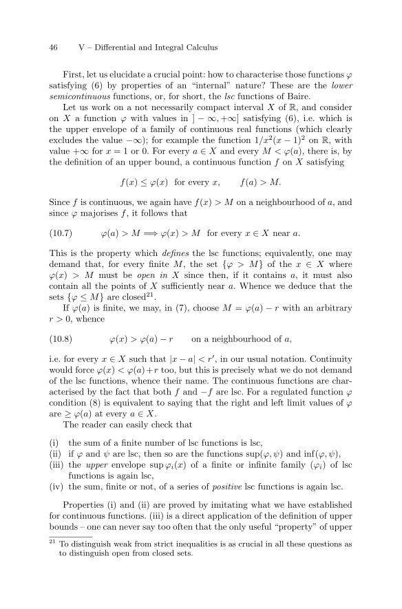
46 V – Differential and Integral Calculus
First, let us elucidate a crucial point: how to characterise those functions ϕsatisfying (6) by properties of an “internal” nature? These are the lowersemicontinuous functions, or, for short, the lsc functions of Baire.
Let us work on a not necessarily compact interval X of R, and consideron X a function ϕ with values in ] − ∞,+∞] satisfying (6), i.e. which isthe upper envelope of a family of continuous real functions (which clearlyexcludes the value −∞); for example the function 1/x2(x − 1)2 on R, withvalue +∞ for x = 1 or 0. For every a ∈ X and every M < ϕ(a), there is, bythe definition of an upper bound, a continuous function f on X satisfying
f(x) ≤ ϕ(x) for every x, f(a) > M.
Since f is continuous, we again have f(x) > M on a neighbourhood of a, andsince ϕ majorises f , it follows that
ϕ(a) > M =⇒ ϕ(x) > M for every x ∈ X near a.(10.7)
This is the property which defines the lsc functions; equivalently, one maydemand that, for every finite M , the set {ϕ > M} of the x ∈ X whereϕ(x) > M must be open in X since then, if it contains a, it must alsocontain all the points of X sufficiently near a. Whence we deduce that thesets {ϕ ≤ M} are closed21.
If ϕ(a) is finite, we may, in (7), choose M = ϕ(a) − r with an arbitraryr > 0, whence
ϕ(x) > ϕ(a) − r on a neighbourhood of a,(10.8)
i.e. for every x ∈ X such that |x − a| < r′, in our usual notation. Continuitywould force ϕ(x) < ϕ(a)+r too, but this is precisely what we do not demandof the lsc functions, whence their name. The continuous functions are char-acterised by the fact that both f and −f are lsc. For a regulated function ϕcondition (8) is equivalent to saying that the right and left limit values of ϕare ≥ ϕ(a) at every a ∈ X.
The reader can easily check that
(i) the sum of a finite number of lsc functions is lsc,(ii) if ϕ and ψ are lsc, then so are the functions sup(ϕ,ψ) and inf(ϕ,ψ),(iii) the upper envelope sup ϕi(x) of a finite or infinite family (ϕi) of lsc
functions is again lsc,(iv) the sum, finite or not, of a series of positive lsc functions is again lsc.
Properties (i) and (ii) are proved by imitating what we have establishedfor continuous functions. (iii) is a direct application of the definition of upperbounds – one can never say too often that the only useful “property” of upper21 To distinguish weak from strict inequalities is as crucial in all these questions as
to distinguish open from closed sets.
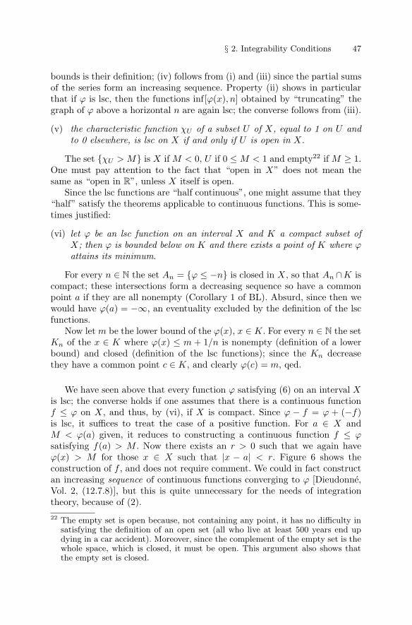
§ 2. Integrability Conditions 47
bounds is their definition; (iv) follows from (i) and (iii) since the partial sumsof the series form an increasing sequence. Property (ii) shows in particularthat if ϕ is lsc, then the functions inf[ϕ(x), n] obtained by “truncating” thegraph of ϕ above a horizontal n are again lsc; the converse follows from (iii).
(v) the characteristic function χU of a subset U of X, equal to 1 on U andto 0 elsewhere, is lsc on X if and only if U is open in X.
The set {χU > M} is X if M < 0, U if 0 ≤ M < 1 and empty22 if M ≥ 1.One must pay attention to the fact that “open in X” does not mean thesame as “open in R”, unless X itself is open.
Since the lsc functions are “half continuous”, one might assume that they“half” satisfy the theorems applicable to continuous functions. This is some-times justified:
(vi) let ϕ be an lsc function on an interval X and K a compact subset ofX; then ϕ is bounded below on K and there exists a point of K where ϕattains its minimum.
For every n ∈ N the set An = {ϕ ≤ −n} is closed in X, so that An ∩K iscompact; these intersections form a decreasing sequence so have a commonpoint a if they are all nonempty (Corollary 1 of BL). Absurd, since then wewould have ϕ(a) = −∞, an eventuality excluded by the definition of the lscfunctions.
Now let m be the lower bound of the ϕ(x), x ∈ K. For every n ∈ N the setKn of the x ∈ K where ϕ(x) ≤ m + 1/n is nonempty (definition of a lowerbound) and closed (definition of the lsc functions); since the Kn decreasethey have a common point c ∈ K, and clearly ϕ(c) = m, qed.
We have seen above that every function ϕ satisfying (6) on an interval Xis lsc; the converse holds if one assumes that there is a continuous functionf ≤ ϕ on X, and thus, by (vi), if X is compact. Since ϕ − f = ϕ + (−f)is lsc, it suffices to treat the case of a positive function. For a ∈ X andM < ϕ(a) given, it reduces to constructing a continuous function f ≤ ϕsatisfying f(a) > M . Now there exists an r > 0 such that we again haveϕ(x) > M for those x ∈ X such that |x − a| < r. Figure 6 shows theconstruction of f , and does not require comment. We could in fact constructan increasing sequence of continuous functions converging to ϕ [Dieudonne,Vol. 2, (12.7.8)], but this is quite unnecessary for the needs of integrationtheory, because of (2).
22 The empty set is open because, not containing any point, it has no difficulty insatisfying the definition of an open set (all who live at least 500 years end updying in a car accident). Moreover, since the complement of the empty set is thewhole space, which is closed, it must be open. This argument also shows thatthe empty set is closed.
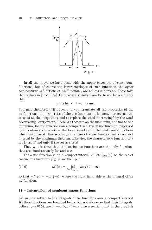
48 V – Differential and Integral Calculus
Fig. 6.
In all the above we have dealt with the upper envelopes of continuousfunctions, but of course the lower envelopes of such functions, the uppersemicontinuous functions or usc functions, are no less important. These taketheir values in [−∞,+∞[. One passes trivially from lsc to usc by remarkingthat
ϕ is lsc ⇐⇒ −ϕ is usc.
You may therefore, if it appeals to you, translate all the properties of thelsc functions into properties of the usc functions: it is enough to reverse thesense of all the inequalities and to replace the word “increasing” by the word“decreasing” everywhere. There is a theorem on the maximum, and not on theminimum, for usc functions on a compact set. Every usc function majorisedby a continuous function is the lower envelope of the continuous functionswhich majorise it; this is always the case of a usc function on a compactinterval by the maximum theorem. Likewise, the characteristic function of aset is usc if and only if the set is closed.
Finally, it is clear that the continuous functions are the only functionsthat are simultaneously lsc and usc.
For a usc function ψ on a compact interval K let Csup(ψ) be the set ofcontinuous functions f ≥ ψ; we then put
m∗(ψ) = inff∈Csup(ψ)
m(f) ≥ −∞,(10.9)
so that m∗(ψ) = −m∗(−ψ) where the right hand side is the integral of anlsc function.
11 – Integration of semicontinuous functions
Let us now return to the integrals of lsc functions over a compact intervalK; these functions are bounded below but not above, so that their integrals,defined by (10.5), are > −∞ but ≤ +∞. The essential point in the proofs is
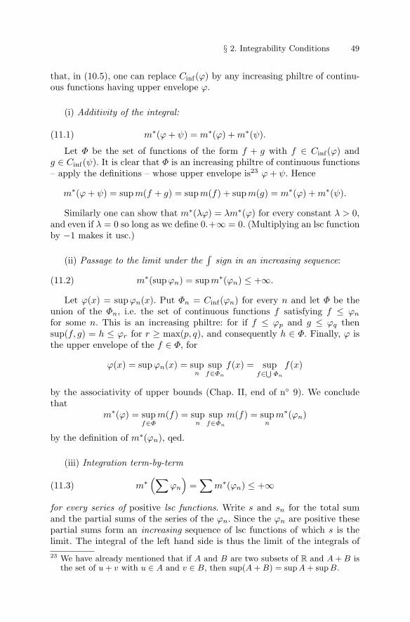
§ 2. Integrability Conditions 49
that, in (10.5), one can replace Cinf(ϕ) by any increasing philtre of continu-ous functions having upper envelope ϕ.
(i) Additivity of the integral:
m∗(ϕ + ψ) = m∗(ϕ) + m∗(ψ).(11.1)
Let Φ be the set of functions of the form f + g with f ∈ Cinf(ϕ) andg ∈ Cinf(ψ). It is clear that Φ is an increasing philtre of continuous functions– apply the definitions – whose upper envelope is23 ϕ + ψ. Hence
m∗(ϕ + ψ) = supm(f + g) = supm(f) + supm(g) = m∗(ϕ) + m∗(ψ).
Similarly one can show that m∗(λϕ) = λm∗(ϕ) for every constant λ > 0,and even if λ = 0 so long as we define 0.+∞ = 0. (Multiplying an lsc functionby −1 makes it usc.)
(ii) Passage to the limit under the∫
sign in an increasing sequence:
m∗(supϕn) = supm∗(ϕn) ≤ +∞.(11.2)
Let ϕ(x) = supϕn(x). Put Φn = Cinf(ϕn) for every n and let Φ be theunion of the Φn, i.e. the set of continuous functions f satisfying f ≤ ϕn
for some n. This is an increasing philtre: for if f ≤ ϕp and g ≤ ϕq thensup(f, g) = h ≤ ϕr for r ≥ max(p, q), and consequently h ∈ Φ. Finally, ϕ isthe upper envelope of the f ∈ Φ, for
ϕ(x) = supϕn(x) = supn
supf∈Φn
f(x) = supf∈⋃ Φn
f(x)
by the associativity of upper bounds (Chap. II, end of n◦ 9). We concludethat
m∗(ϕ) = supf∈Φ
m(f) = supn
supf∈Φn
m(f) = supn
m∗(ϕn)
by the definition of m∗(ϕn), qed.
(iii) Integration term-by-term
m∗(∑
ϕn
)=∑
m∗(ϕn) ≤ +∞(11.3)
for every series of positive lsc functions. Write s and sn for the total sumand the partial sums of the series of the ϕn. Since the ϕn are positive thesepartial sums form an increasing sequence of lsc functions of which s is thelimit. The integral of the left hand side is thus the limit of the integrals of23 We have already mentioned that if A and B are two subsets of R and A + B is
the set of u + v with u ∈ A and v ∈ B, then sup(A + B) = sup A + sup B.
50 V – Differential and Integral Calculus
the sn by (ii), i.e., by (i), of the partial sums of the series of the integrals,qed. Note that if the ϕn are not positive the sum of the series need not evenbe lsc.
If, in particular, the functions ϕn satisfy m∗(ϕn) < +∞, i.e. are m-integrable (by definition), and if
∑m∗(ϕn) < +∞, then the sum of the series
is again integrable and one may integrate it term-by-term. In particular, forpositive lsc functions,
m∗(ϕn) = 0 for every n =⇒ m∗(∑
ϕn
)= 0.(11.4)
Since the characteristic function of an open set U in K is lsc one maydefine the measure of an open set by putting
m(U) = m∗(χU ),(11.5)
a number clearly lying between 0 and m(K); it is clear more generally that
U ⊂ V =⇒ m(U) ≤ m(V )(11.6)
since then χU ≤ χV . It is easy to see that, when U is an interval, m(U) reducesto its usual length; for this obviously majorises m(f) for every continuousfunction f ≤ χU (i.e. ≤ 1 on U and ≤ 0 elsewhere), but on replacing thediscontinuities of the graph of the characteristic function at the end-pointsof U by almost vertical line segments joining 0 to 1, one constructs functionsf whose integral is arbitrarily close to the length of U .
Properties (i), (ii) and (iii) above translate immediately:
(i’) if U and V are open in K then m(U ∪ V ) ≤ m(U) + m(V ) and
m(U ∪ V ) = m(U) + m(V ) if U and V are disjoint.(11.7)
Obvious, since, in the last case, we have χU∪V = χU + χV .
(ii’) if (Un) is an increasing sequence of open sets then
m(⋃
Un) = limm(Un) = supm(Un).(11.8)
Obvious since the characteristic function of the union is the limit of the se-quence, increasing, of those of the Un.
(iii’) if (Un) is any sequence of open sets then
m(∑
Un
)≤∑
m(Un)(11.9)
with equality if the Un are pairwise disjoint.
§ 2. Integrability Conditions 51
Obvious, since the characteristic function of the union is less than the sum ofthe characteristic functions of the Un and is equal to it if the Un are pairwisedisjoint.
This allows us to calculate the measure of any open U ⊂ K explicitly.First, note that for every a ∈ U the union of all the intervals containing aand contained in U is again an interval U(a), clearly open in K like U itself,and of length > 0; U is the union of these U(a). It is immediate that, fora �= b, either U(a) = U(b) or U(a)∩U(b) = ∅. The set (and not the family) ofthe U(a) is countable, for those of these intervals which are of length > 1/pare at most m(K)p in number since they are pairwise disjoint. Thus we seethat every open subset U of K (and, in fact, of any interval, compact or not,and in particular of R) is the union of a finite or countable family of openpairwise disjoint intervals. The measure of U is then, by (iii’), the sum of themeasures of these intervals.
We leave the reader the task of translating all these properties into termsof usc functions and of closed sets. To go further along this path wouldoblige us to develop all the Lebesgue theory. The reader may find theseconsiderations insufficient: for, at this point of the exposition, (i) we are notyet able to integrate the difference of two lsc functions for the reason that itis neither lsc nor usc24, (ii) we have considered integrals only over compactintervals. These limitations will be removed in the Appendix to this Chapter.
Exercise. We say that a set N ⊂ K is of measure zero if, for every r > 0there is an open U ⊂ N such that m(U) < r. (i) Show that the union of afinite or denumerable family of sets of measure zero is of measure zero (usethe fact that r =
∑r/2n). Show that Q∩K is of measure zero. (ii) Let ϕ be a
positive lsc function such that m∗(ϕ) < +∞; show that the set {ϕ(x) = +∞}is of measure zero (use the sets {ϕ(x) > n}.
24 The ingenious reader will observe that if ϕ′, ϕ′′, ψ′ and ψ′′ are lsc functionswith finite values such that ϕ′ − ψ′ = ϕ′′ − ψ′′, then ϕ′ + ψ′′ = ϕ′′ + ψ′, som(ϕ′) + m(ψ′′) = m(ϕ′′) + m(ψ′), so m(ϕ′) − m(ψ′) = m(ϕ′′) − m(ψ′′). Onemay thus define m(θ) = m(ϕ′) − m(ψ′) without ambiguity for every function θwhich can be expressed in the form of a difference of two positive lsc functionswith finite values. These functions form a vector space over R, etc. But this isnot the best method for obtaining the general integrable functions: we still lack“almost everywhere zero” functions.
52 V – Differential and Integral Calculus
§ 3. The “Fundamental Theorem” (FT)
12 – The fundamental theorem of the differential and integral cal-culus
Let us return to much more elementary considerations and introduce thenotion of an oriented integral, analogous to that of a vector on a line. To dothis, first observe that we always have∫ b
a
f(x)dx +∫ c
b
f(x)dx =∫ c
a
f(x)dx(12.1)
if a ≤ b ≤ c. This is geometrically obvious, and has been proved in n◦ 2,additivity formula (2.8).
(1) shows that ∫ c
b
=∫ c
a
−∫ b
a
;
we may then write this relation in the form∫ c
b
=∫ a
b
+∫ c
a
agreeing that ∫ v
u
f(x)dx = −∫ u
v
f(x)dx if u > v.(12.2)
As in the case of the vectors, the relation (1) remains valid with no hypothesison the respective positions of a, b and c.
Having said this, let f be a scalar function defined on an interval I (ofany kind), and assume that f has right and left limits at each point of I, i.e.that f is regulated. We may then, for a given a ∈ I, consider the function
F (x) =∫ x
a
f(t)dt(12.3)
on I, with an oriented integral in the preceding sense, so the opposite ofthe ordinary integral for x < a. We have denoted the phantom variable ofintegration by t so as not to confuse it with the variable x in F ; one canreplace t by y, u, $ or anything one likes, except x, f or d . . .
By the properties of oriented integrals
F (x + h) − F (x) =∫ x+h
x
f(t)dt.
This relation shows first of all that F is continuous: since f is bounded onevery compact interval K ⊂ I, the preceding integral is O(h) when h tendsto 0.
§ 3. The “Fundamental Theorem” (FT) 53
If, on the other hand, h is > 0 and small enough, then the function f is,on ]x, x + h], almost equal to the limit value f(x+), so that its integral isalmost equal to hf(x+) since the value taken by f at the point x, or at anyother individual point, has no influence on that of the integral; the quotient[F (x+h)−F (x)]/h is therefore almost equal to f(x+), so tends to this limitas h > 0 tends to 0.
Weierstrass’s Epsilontik is missing from this argument. To introduce it,first observe that ∫ x+h
x
f(x+)dt = hf(x+)
because f(x+) is not a function of the variable of integration t, in otherwords, behaves like a constant function of t for x given. (Whence, once more,the necessity of not mixing the phantom or bound variables like t and thefree variables like x.) Then
F (x + h) − F (x)h
− f(x+) =1h
∫ x+h
x
[f(t) − f(x+)]dt.(12.4)
Now for every r > 0, there exists an r′ > 0 such that
x < t ≤ x + r′ =⇒ |f(t) − f(x+)| ≤ r.
The right hand side of (4) is then, in modulus, ≤ r. We argue similarly forh < 0, replacing the interval ]x, x + r′[ by an interval ]x − r′′, x[ and f(x+)by f(x−). The left hand side then tends to 0, whence:
Theorem 11. Let f be a regulated function on an interval I in R. Then thefunction F defined by the relation (3) is continuous and has right and leftderivatives equal to f(x+) and f(x−) at each point x ∈ I.
This result, for functions as then understood, is already in Newton in1665–66 with essentially the same proof, phrased in his language of fluentesand fluxions (Chap. III, n◦ 14): if y is the fluent which defines the curve[y = f(x) in the language of today] and if z is the area [i.e. the integral]between a fixed abscissa and the abscissa of the fluent x, then the infinitesi-mal increase zo of z is the product of y by the infinitesimal increase xo of x,which means that z/x = y; if one assumes that x = 1, in other words thatx is the “time” with respect to which one derives one’s fluentes to calculatetheir fluxions, one has z = y, which, even in his conception of derivatives as“speeds of variation in time”, means that the derivative of the area z withrespect to the variable x is the ordinate y of the graph at the point x; inLeibniz’ style, dz/dx = y. For them, calculating the area is the same as cal-culating a fluent z satisfying this relation. Newton justifies nothing, not eventhe fact that the relation z = y determines z up to an additive constant,which is, however, the crucial point; a few lines suffice for him to formulate
54 V – Differential and Integral Calculus
his result25 which he illustrates by examples. Chez Leibniz, everything is sim-ple too: since F (x) is the “continuous sum” of the infinitely small quantitiesf(t)dt where t varies from the left hand end of the area to x, the infini-tesimal increase in F when one passes from x to x + dx is f(x)dx, whencedF = f(x)dx and f(x) = dF/dx. Here again, the justifications awaited theXIXth century, but since the method worked admirably, for 150 years no onebothered to provide the rigorous proofs by “exhaustion” of Chap. II, n◦ 11 . . .
Recall that the set D of discontinuities of a regulated function f is finiteor countable (Theorem 6 or Chap. III, n◦ 12). Outside D the function F istherefore differentiable, with F ′(x) = f(x).
When the function f is continuous, the function F is even differentiableon all the interval considered, and
F ′(x) = f(x) for every x(12.5)
in this case. One says then that F is a primitive of f . These arguments provethe existence of a primitive for every continuous function. This result is notat all clear for a function which, though continuous, may be so savage thatone cannot represent it graphically.
Now, in contrast to Newton, who did not even pose the question since hedid not see (and one still does not see it . . .) how a graph all of whose tangentsare horizontal could be anything other than a line, we know (Chap. III, n◦ 16)that if two everywhere differentiable functions on an interval have the samederivatives everywhere, then their difference is constant. Since the additionof a constant to the function F defined by (3) does not change the differenceF (x) − F (a), we obtain the following result:
Theorem 12 (FT). Let f be a scalar function defined and continuous onan interval I in R and let F be a primitive of f , i.e. a differentiable functionsuch that F ′(x) = f(x) for every x ∈ I. Then
∫ b
a
f(x)dx = F (b) − F (a)(12.6)
for any a, b ∈ I.
In this way we find the results of n◦ 4, Example 1, again, for analyticfunctions, but in a much more general framework.
Example 1. For x > 0 and s ∈ C, the function
xs = exp(s. log x)
25 Tractatus de Methodis Serierum et Fluxionum, pp. 195–197 and 211 of Vol. IIIof the Mathematical Papers.
§ 3. The “Fundamental Theorem” (FT) 55
has derivative sxs−1 [Chap. IV, formula (10.10)]. The function xs+1/(s + 1)is therefore, for s �= −1, a primitive of xs. Whence the formula∫ b
a
xsdx =bs+1 − as+1
s + 1(0 < a, b; s ∈ C, s �= −1)(12.7)
already obtained for s ∈ N by a direct calculation of the integral (Chap. II,n◦ 11), but now valid for any s ∈ C, s �= 1.
Example 2. For x > 0 the function log x has derivative 1/x; hence again theformula ∫ b
a
dx/x = log b − log a (0 < a, b)
of Chap. II, n◦ 11.
Example 3. The derivative of the function arctanx is 1/(1 + x2); whence∫ b
a
dx
1 + x2= arctan b − arctan a;
we must pay attention to the fact that, in this calculation, we take the “prin-cipal determination” of arctanx, that given by the relation
y = arctan x ⇐⇒ {(x = tan y) & (|y| < π/2)}or, equivalently, the inverse function of
tan : ] − π/2, π/2[ −→ R.
Example 4. For c ∈ C, c �= 0, the derivative of ecx/c is ecx; we again find theformula ∫ b
a
ecxdx = (ecb − eca)/c.
In practice, we often use the notation
F (b) − F (a) = F (x)∣∣∣ba;(12.8)
this contradicts all the most elementary rules of mathematical logic with itsx which might be a t, a # or a £ and which, despite its clearly phantomcharacter, is not linked visibly to any of its occurrences. It would be morecorrect to write
F (x)∣∣∣∣ x = b
x = aor even F (�)
∣∣∣∣ � = b� = a
,
especially when F depends on several variables x, y, etc. But as we have saidalready, one does not change society, even mathematical society, by ukase.
56 V – Differential and Integral Calculus
To denote a primitive of f , there is another notation, long universal, andeven more catastrophic, namely
F (x) =∫
f(x)dx,
omitting the limits of integration. Since the letter x on the right hand sidedenotes a bound variable and that on the left hand side a free variable, all thetabus are violated26. The inventors of this system probably knew what theywere doing; Leibniz printed it for the first time in 1686 in his aptly namedGeometria recondita, and for example wrote that∫
xdx = x2/2,
the word “integral” being introduced by Jakob Bernoulli in 1690 (Cantor,pp. 197, 218). But their principal reason is that they were much more con-cerned to calculate primitives rather than integrals between well defined lim-its, and, as we have already said, one had to wait for Fourier for the idea ofdisplaying the integration limits in the integral notation. Imagine the con-fusions that this system must have provoked among less brilliant people, ifnot chez Leibniz, the Bernoullis or Euler – brains of this calibre are not borneveryday. Not to ignore that relations such as∫
cos x.dx = sin x,
∫dx/x = log x,
etc. may induce the same confusions even nowadays. . .
Another way of formulating the preceding theorem starts from a functionf of class C1, i.e. having a continuous derivative. Since f is a primitive of f ′
one finds the relation
f(b) − f(a) =∫ b
a
f ′(x)dx,(12.9)
as fundamental as the FT, for any a and b in the interval I considered, or,in the language of indefinite integrals,
f(x) =∫
f ′(x)dx,(12.10)
26 We shall use this notation frequently, and have already used it, though in quiteanother context, namely to denote an integral extended over an interval men-tioned repeatedly in the calculations, and where no ambiguity is possible. Thisconvention or abbreviation, which often allows us to write the integrals in thebody of the text in clear language instead of using an extra line each time,economises on type and paper.
§ 3. The “Fundamental Theorem” (FT) 57
or even f(x) =∫
df(x). In this form, the reciprocity between derivativeand integral appears clearly. In the version (9) one chooses a subdivisiona = x1 ≤ x2 ≤ . . . ≤ xn+1 = b of [a, b], writes that
f(b) − f(a) =∑
[f(xi+1) − f(xi)](12.11)
and observes that the difference f(xi+1) − f(xi) is “almost” equal tof ′(xi)(xi+1 − xi) and, in fact, exactly equal to f ′(ξi)(xi+1 − xi) for someξi ∈]xi, xi+1[ by the mean value theorem if f is real. Substituting in theabove expression for f(b)− f(a), one finds exactly the Riemann sums whichdefine the integral (9). This type of argument was clearly known to Leibniz;it is linked to “the calculus of finite differences” so popular in the XVIIth
and XVIIIth centuries. Leibniz’ notation makes these results as intuitive asthey must have been almost obvious in the eyes of the contemporaries whodid not worry about arithmetising analysis, whence their popularity.
The formula (9) explains Theorem 19 of Chap. III, n◦ 17 on differentiatinga uniform limit. Suppose we are given a sequence of functions fn of class C1
on an interval I, and assume that the f ′n converge to a limit g uniformly on
every compact K ∈ I. Then, by Theorem 4 of n◦ 4,∫ x
a
g(t)dt = lim∫ x
a
f ′n(t)dt = lim[fn(x) − fn(a)](12.12)
for any a, x ∈ I. If the sequence fn converges at the point a, it must thenconverge everywhere to a function f , which, satisfying
f(x) − f(a) =∫ x
a
g(t)dt(12.13)
by (12), is a primitive of g; in other words, the derivative of the limit is thelimit of the derivatives. An immediate estimate of the integral of g− f ′
n thenshows that the sequence fn converges uniformly on every compact set. ButTheorem 19 of Chap. III only assumes the existence of the f ′
n, and not theircontinuity.
We established a theorem on “differentiation under the∫
sign” for inte-grals of the form
∫f(x, y)dx above. We may combine this with the FT to
obtain the following occasionally useful result:
Theorem 13. Let I and J be two intervals, f a continuous function on I×Jand let ϕ,ψ : I → J be two differentiable functions. Suppose that f has acontinuous derivative D1f on I × J . Then the function
g(x) =∫ ψ(x)
ϕ(x)
f(x, y)dy(12.14)
is differentiable on I, and
g′(x) =∫ ψ(x)
ϕ(x)
D1f(x, y)dy + f [x, ψ(x)]ψ′(x) − f [x, ϕ(x)]ϕ′(x).(12.15)
58 V – Differential and Integral Calculus
By subtracting, one need only prove this in the case where ϕ(x) = b isconstant. Put
F (x, y) =∫ y
b
f(x, t)dt,
whence g(x) = F [x, ψ(x)]. Since f is continuous the FT shows that
D2F (x, y) = f(x, y).(12.16)
Theorem 9 shows on the other hand that
D1F (x, y) =∫ y
b
D1f(x, t)dt.(12.17)
By Theorem 9 (i) D1F is continuous on I × J , and since D2F = f is alsocontinuous we see that F is a function of class C1 on I × J . We may thusapply the chain rule to g(x) = F [x, ψ(x)] (Chap. III, n◦ 21), whence
g′(x) = D1F [x, ψ(x)] + D2F [x, ψ(x)]ψ′(x);
one obtains the desired formula on substituting ψ(x) for y in (16) and (17).
Exercise. By the theorem, the function
g(x) =∫ x3
x2sin(xy)dy
has derivative
g′(x) =∫ x3
x2cos(xy)ydy + 3x2 sin(x4) − 2x sin(x3).
Check this result by calculating the integrals that appear in g and g′ (for thesecond, integrate by parts).
Exercise. Prove (15) directly by writing
g(x + h) − g(x) =∫ ψ(x+h)
b
f(x + h, y)dy −∫ ψ(x)
b
f(x, y)dy.
Since we have just made a new incursion into the functions of two realvariables, let us show how one may exploit the FT to establish one of thefundamental results of Chap. III, n◦ 23:
Theorem 14. Let f(x, y) be a function defined and continuous on I × Jwhere I and J are two intervals in R. Assume that f has continuous secondderivatives D1D2f and D2D1f on I × J . Then they are equal.
§ 3. The “Fundamental Theorem” (FT) 59
Since it is enough to verify the statement on a neighbourhood of an ar-bitrary point of I × J one may reduce to the case where I = [a, b] andJ = [c, d] are compact. The FT applied to the functions y → D2D1f(x, y)and x → D1f(x, y) then shows that∫ u
a
dx
∫ v
c
D2D1f(x, y)dy =(12.18) ∫ u
a
[D1f(x, v) − D1f(x, c)] dx = f(x, v) − f(x, c)∣∣∣∣x=u
x=a
for any u ∈ I and v ∈ J . A similar calculation will show that∫ v
c
dy
∫ u
a
D1D2f(x, y)dx = f(u, y) − f(a, y)∣∣∣∣y=v
y=c
,(12.19)
a result obviously identical to that furnished by (18). But we already knowthat the order of integration is unimportant in these double integrals. Putting
g(x, y) = D2D1f(x, y) − D1D2f(x, y),
we thus obtain a continuous function on I × J such that∫ u
a
dx
∫ v
c
g(x, y)dy = 0(12.20)
for any u ∈ I and v ∈ J . On differentiating with respect to u one finds thatthe integral of g(x, y) between c and v is zero for any v. On differentiatingwith respect to v, one obtains g(x, y) = 0, qed. [Note that Chap. III, n◦ 23,only requires D1f and D2f to be differentiable at the point (x, y) considered].
13 – Extension of the fundamental theorem to regulated functions
Let us return to the usual integral and to the “fundamental theorem”. Thehypothesis that f is of class C1 is not indispensable in justifying formula(12.9); it still holds if, for example, f ′(x) is a regulated function. For this, andas N. Bourbaki and also Dieudonne (Elements d’analyse, Vol. 1, Chap. VIII,n◦ 7) do, let us say that for a regulated function f defined on an arbitraryinterval I any continuous function F which has a derivative equal to f(x)outside a countable subset D of I is a primitive of this regulated function.
Theorem 12 bis. Let f be a regulated function on an interval I ⊂ R. Then(i) f has a primitive F in I; (ii) any two primitives of f are equal up to anadditive constant; (iii) we have∫ b
a
f(x)dx = F (b) − F (a)
for any a, b ∈ I; (iv) every primitive F of f has right and left derivativesF ′
d(x) = f(x+), F ′g(x) = f(x−) at every point.
60 V – Differential and Integral Calculus
Point (i) follows from Theorem 11: the continuous function F of Theo-rem 11 satisfies (iv) and since f is continuous outside a countable set D, Fhas a derivative F ′(x) = f(x) for x /∈ D.
Since (iii) is valid for a particular primitive, (iii) will be established if weprove (ii), in other words that a continuous function having a zero derivativeoutside a countable set D is constant. For this it is enough to show that ifthe derivative is ≥ 0 outside D, then the function is increasing, for a functionwhich is simultaneously increasing and decreasing has no choice.
We shall give two rather different and extremely ingenious proofs of thistheorem27.
It is enough to establish this result when f ′(x) is strictly positive every-where on I−D, since if f(x)+εx, which satisfies this hypothesis, is increasingfor every ε > 0, then so clearly is f in the limit. One may also restrict oneselfto examining the case where I is compact, since, to show that a ≤ b impliesf(a) ≤ f(b), it is enough to argue on the interval [a, b].
The basic idea is that the ratio [f(x+h)−f(x)]/h is > 0 for h small enoughsince it tends to f ′(x) > 0; then f(x) < f(x+h) for every small enough h > 0;it remains to pass from “locally” increasing to “globally”increasing, which theFounding Fathers considered obvious.
First proof. Assume that f ′(x) > 0 for x ∈ I − D. If f is not increasing,there exist points c, d of I such that c < d, f(c) > f(d). For every numberξ ∈ ]f(d), f(c)[, the equation f(x) = ξ has at least one solution between cand d (intermediate value theorem). The set E(ξ) of these solutions is closedsince f is continuous, and it is bounded since ⊂ [c, d]; it therefore containsthe number supE(ξ) = dξ, and we have dξ < d since f(dξ) = ξ > f(d).
Let us show that if h > 0 is small enough that dξ +h < d then f(dξ +h) <f(dξ) = ξ. If in fact f(dξ + h) ≥ ξ, a number > f(d), then the equationf(x) = ξ would have a solution between dξ+h and d; absurd since sup E(ξ) =dξ < dξ + h.
It follows from this that, for every ξ ∈ ]f(d), f(c)[ and every sufficientlysmall h > 0,
[f(dξ + h) − f(dξ)]/h < 0.
This is impossible if the derivative f ′(dξ) (or even only the right derivative)exists, since by hypothesis it is > 0; the function f is thus not differentiableat any of the points dξ, which proves that dξ ∈ D.
Now the map ξ → dξ of ]f(d), f(c)[ in D is injective because
27 I find the first in Walter, Analysis I, pp. 354–359, who attributes it to L. Scheef-fer, 1885, the date when arguments a la Cantor began to be fashionable. Forthe second I have simplified the method of Dieudonne, Elements . . ., Vol. 1,Chap. VIIII, n◦ 6, which treats the case of functions with values in Banachspaces, and could in fact be deduced from the result for real-valued functionswith the help of the Hahn-Banach theorem. Both authors prove the mean valuetheorem, below, directly.
§ 3. The “Fundamental Theorem” (FT) 61
ξ �= η =⇒ f(dξ) = ξ �= η = f(dη) =⇒ dξ �= dη.
If the theorem were false we would have constructed an injective map of aninterval ]f(d), f(c)[ of R into a countable set, absurd if one believes Cantor . . .
As we have seen in passing, it would suffice, to obtain (2), to assume thatf has a positive right derivative outside D. The same remark applies to theproof that follows.
Second proof. Here again we reduce to showing that f(a) ≤ f(b) iff ′(x) > 0 on I = [a, b].
Let us first explain the method in the simplest case (already explainedin another way in Chap. III, n◦ 16) where f is differentiable for every x ∈ Iwithout exception. The set E of the x ∈ [a, b] such that f(a) ≤ f(x) containsa and is closed since f is continuous. Let c = sup(E) ≤ b, whence c ∈ E;assume that c < b. For all x > c near enough to c, one has f(x) > f(c) ≥ f(a)since f ′(c) > 0, whence x ∈ E if x ∈ I. If c < b then E contains pointsx > c = sup(E), absurd. Whence c = b, qed.
Now let us pass to the general case, where the derivative exists onlyoutside D. First notice that if f(u) ≥ f(a) at a point u ∈ [a, b], then againf(x) > f(u) [and so > f(a)] for every x > u close enough to u if f ′(u) exists;in the contrary case, one may only guarantee, for every ε > 0, that one hasf(x) > f(u)− ε [and so > f(a)− ε] for every x > u near enough to u since fis continuous. This indicates that if one moves from a to b, one is forced, inseeking to prove the inequality f(x) ≥ f(a), to subtract an error term fromf(a) each time that one meets a point of D. If one can contrive that the sumof these errors will be ≤ r when one arrives at the point b, one obtains theinequality f(b) ≥ f(a) − r, which, valid for every r > 0, proves the theorem.
One must therefore, for each ξ ∈ D, allow an error r(ξ) chosen so that∑r(ξ) ≤ r. Since D is finite or countable, one need only write the points of
D in the form of a sequence (ξn) and choose, for example, r(ξn) = r/2n. Wewill find this technique again in the Lebesgue theory.
Let us now pass on to the formal proof. We denote by E the set of x ∈ [a, b]satisfying the relation
f(x) ≥ f(a) −∑ξ<x
r(ξ) = g(x);(13.1)
the series converges since it is a subseries of a convergent series of positiveterms. All we have to prove is that b ∈ E.
The first claim to make is that the function g defined by the right handside of (1) is decreasing: for y < x, the ξ < y are themselves < x; consequently,g(x) is obtained by subtracting from g(y) the numbers r(ξ) > 0 for the ξ ∈ Dsuch that x ≥ ξ > y. This argument even shows that
x > y =⇒ g(x) ≤ g(y) − r(y),(13.2)
62 V – Differential and Integral Calculus
agreeing to put r(y) = 0 if y /∈ D.Now, as above, let c = sup(E); we show first that c ∈ E. For every x ∈ E
we have x ≤ c and so g(x) ≥ g(c), whence f(x) ≥ g(x) ≥ g(c); since c is thelimit of points of E, we also have f(c) ≥ g(c) since f is continuous.
It remains to prove that c = b. Now assume that c < b, and let us considerthe x ∈ ]c, b]. There are two possible cases.
(i) f is differentiable at c. If x is near enough to c, we have on the onehand that f(x) > f(c) since f ′(c) > 0, and on the other hand g(x) ≤ g(c)since x > c; whence, for these x, f(x) > f(c) ≥ g(c) ≥ g(x) and so x ∈ E;absurd since sup(E) = c < x.
(ii) f is not differentiable at c, i.e. c ∈ D. For c < x ≤ b, one hasf(x) < g(x) because x /∈ E. Since c < x, we have g(x) ≤ g(c) − r(c) by (2).Thus f(x) < g(c) − r(c). But g(c) ≤ f(c) since c ∈ E, see (1). Consequently
c < x ≤ b =⇒ f(x) < f(c) − r(c);
since r(c) > 0 because c ∈ D, this relation contradicts the continuity of f atthe point c if c < b, qed.
As we have said, most authors deduce the preceding results from a state-ment which appears more general and which we have already met for every-where differentiable functions:
Mean value theorem. Let f be a scalar function defined and continuouson an interval I ⊂ R; assume that f is differentiable at every point of I −D,where D is a countable subset of I. Then, for any a, b ∈ I with a ≤ b,
|f(b) − f(a)| ≤ M(b − a)(13.3)
where M ≤ +∞ is the upper bound of |f ′(x)| on the interval [a, b].
First assume that the function f is real and that, for x ∈ [a, b], f ′(x) hasits values in a compact interval [m,M ] (there is nothing to prove if f ′ is notbounded in [a, b]); we show that then
m(y − x) ≤ f(y) − f(x) ≤ M(y − x)(13.4)
for a ≤ x ≤ y ≤ b. Now this means that the function f(x)−mx is increasingand the function f(x) − Mx is decreasing in [a, b]. The derivatives of thesefunctions being respectively positive and negative outside D, we can writethe final qed in the real case.
The case of a function f with complex values reduces to the precedingcase by an artifice already employed in the same context [Chap. III, n◦ 16,proof of (16.5)]: one applies the result already established for real functionsto the function fz(x) = Re[zf(x)], where z is an arbitrary complex constant;its derivative Re[zf ′(x)] lies, outside D, between −M |z| and M |z| whereM = sup |f ′(x)|, so that
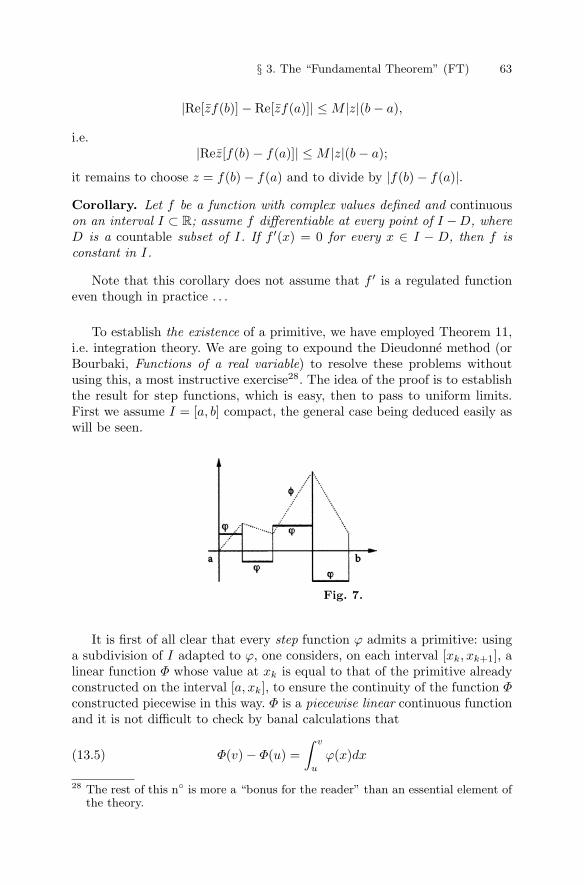
§ 3. The “Fundamental Theorem” (FT) 63
|Re[zf(b)] − Re[zf(a)]| ≤ M |z|(b − a),
i.e.|Rez[f(b) − f(a)]| ≤ M |z|(b − a);
it remains to choose z = f(b) − f(a) and to divide by |f(b) − f(a)|.Corollary. Let f be a function with complex values defined and continuouson an interval I ⊂ R; assume f differentiable at every point of I −D, whereD is a countable subset of I. If f ′(x) = 0 for every x ∈ I − D, then f isconstant in I.
Note that this corollary does not assume that f ′ is a regulated functioneven though in practice . . .
To establish the existence of a primitive, we have employed Theorem 11,i.e. integration theory. We are going to expound the Dieudonne method (orBourbaki, Functions of a real variable) to resolve these problems withoutusing this, a most instructive exercise28. The idea of the proof is to establishthe result for step functions, which is easy, then to pass to uniform limits.First we assume I = [a, b] compact, the general case being deduced easily aswill be seen.
Fig. 7.
It is first of all clear that every step function ϕ admits a primitive: usinga subdivision of I adapted to ϕ, one considers, on each interval [xk, xk+1], alinear function Φ whose value at xk is equal to that of the primitive alreadyconstructed on the interval [a, xk], to ensure the continuity of the function Φconstructed piecewise in this way. Φ is a piecewise linear continuous functionand it is not difficult to check by banal calculations that
Φ(v) − Φ(u) =∫ v
u
ϕ(x)dx(13.5)
28 The rest of this n◦ is more a “bonus for the reader” than an essential element ofthe theory.
64 V – Differential and Integral Calculus
for any u, v ∈ I. Even if one ignores, in the French or English sense, the meanvalue theorem, which would allow one to show that the preceding constructionprovides all the primitives29 of ϕ, it provides, for every step function ϕ, atleast one standard primitive defined up to an additive constant. This is theone we shall use in the course of the proof, and for good reason, since thereis nothing else!
With this convention, by (5)
|Φ(u) − Φ(v)| ≤ ‖ϕ‖I .|u − v|(13.6)
for any u, v ∈ I.To pass from this to the case of an arbitrary regulated function f one
chooses a sequence of step functions ϕn converging to f uniformly on I = [a, b]and, for each n, a primitive Φn of ϕn; since we obviously want the Φn toconverge to a primitive of f , it is prudent to impose the condition Φn(a) = 0.We shall show that the functions Φn converge uniformly on I to a primitiveF of f , which will prove its existence.
Now the piecewise linear function Φpq = Φp−Φq is a primitive of the stepfunction ϕpq = ϕp − ϕq. By (6) for v = a we have
|Φpq(u)| ≤ ‖ϕpq‖I .(u − a) ≤ m(I)‖ϕpq‖I(13.7)
for every u ∈ I, whence ‖Φp − Φq‖I ≤ m(I)‖ϕp − ϕq‖I , which shows thatthe Φn satisfy Cauchy’s criterion. Hence their uniform convergence to a limitfunction F , continuous like the Φn.
We must now prove that F ′(x) = f(x) outside a countable set of pointsof I. Of course there is Theorem 19 of Chap. III, n◦ 17, but that assumesthe ϕn to be differentiable everywhere, which is not the case here exceptoutside a finite set Dn ⊂ I for each n. Outside the union D of the Dn onemay imitate the proof of the theorem in question, Theorem 19, the essentialbeing, in the present notation, to show that at every point t /∈ D one has arelation analogous to formula (17.4) of Chap. III:
limx→t
limn→∞
Φn(x) − Φn(t)x − t
= limn→∞ lim
x→t
Φn(x) − Φn(t)x − t
;(13.8)
on the left hand side the limit over n is [F (x)−F (t)]/(x−t), so that the limitover x, if it exists, must be F ′(t); on the right hand side the limit over x isthe derivative in t of Φn, i.e. ϕn(t), which exists since we are outside D anda fortiori outside Dn, so that the limit over n is f(t); whence F ′(t) = f(t)modulo proving (8).
We have to argue as in Chap. III, i.e. to apply Theorem 16 of n◦ 12 onthe “limits of limits”. Again we put (for a given t)29 Note that while it is easy to construct a primitive of a step function “without
knowing anything”, to show that it is unique up to a constant reduces, even inthis particularly elementary case, to proving that a function with everywherezero derivative is constant.
§ 3. The “Fundamental Theorem” (FT) 65
cn = Φ′n(t), un(x) = [Φn(x) − Φn(t)]/(x − t),
u(x) = [F (x) − F (t)]/(x − t)
and work on the set X = I − (D ∪ {t}) obtained by omitting from I on theone hand the points of D where the Φn are not all differentiable, on the otherhand the point t where the quotients (8) are meaningless30. We know thatun(x) tends to cn when x → t, and that un(x) tends to u(x) for every x ∈ Iwhen n → +∞. To deduce that the cn tend to a limit c and that u(x) tendsto c when x → t, it is enough to show that the un converge to u uniformlyon X and, for this, to verify the corresponding Cauchy criterion. But againputting Φpq = Φp − Φq, ϕpq = ϕp − ϕq, the general relation (6) shows that
|Φpq(x) − Φpq(t)| ≤ ‖ϕpq‖I .|x − t| = ‖ϕp − ϕq‖I .|x − t|.Since clearly
up(x) − uq(x) = [Φpq(x) − Φpq(t)]/(x − t),
it follows that
|up(x) − uq(x)| ≤ ‖ϕp − ϕq‖I for every x ∈ X,
and thus ‖up − uq‖X ≤ ‖ϕp − ϕq‖I . Hence the uniform convergence of theun on X. The relation (8) is thus justified at every point where the limitsappearing on the right hand side of (8) exist, i.e. on I − D.
Since, what is more, the relation (5) is valid for every ϕn, it is clear thatit is also valid for f and F by passage to the uniform limit. This finishes theproof in the case of a compact interval I.
The case of a noncompact interval I reduces to this immediately. Onechooses a point a ∈ I and writes I =
⋃In where the In are compact intervals
containing a and such that In ⊂ In+1. On each In the function f has aprimitive Fn such that Fn(a) = 0, unique since F ′ = 0 implies F = consteven if F ′(x) does not exist on the points of a countable set. Thus Fn = Fn+1
on In for any n, whence the existence on I of a function F which, on eachIn, coincides with Fn. It is clear that F satisfies Theorem 9 bis, etc.
14 – Convex functions; Holder and Minkowski inequalities
Let a and b be two distinct points in a Cartesian space Rp. A point x ∈ Rp
lies on the line joining a and b if and only if the vector x − b is proportionalto the vector a − b, i.e. x − a = t(b − a) or
x = (1 − t)a + tb(14.1)30 Note in passing the usefulness of defining uniform convergence for functions
defined on any set, and not only on an interval of R. Nor is it any more difficult. . .
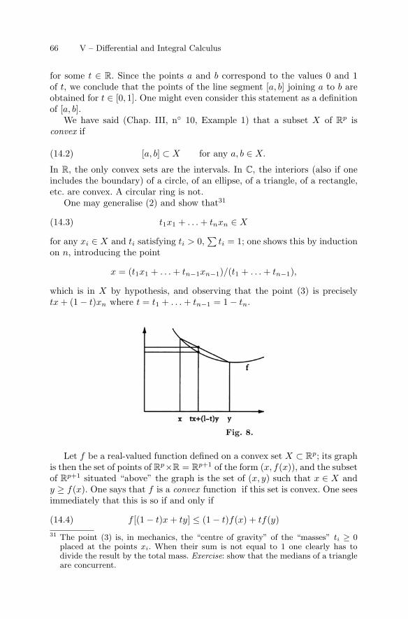
66 V – Differential and Integral Calculus
for some t ∈ R. Since the points a and b correspond to the values 0 and 1of t, we conclude that the points of the line segment [a, b] joining a to b areobtained for t ∈ [0, 1]. One might even consider this statement as a definitionof [a, b].
We have said (Chap. III, n◦ 10, Example 1) that a subset X of Rp isconvex if
[a, b] ⊂ X for any a, b ∈ X.(14.2)
In R, the only convex sets are the intervals. In C, the interiors (also if oneincludes the boundary) of a circle, of an ellipse, of a triangle, of a rectangle,etc. are convex. A circular ring is not.
One may generalise (2) and show that31
t1x1 + . . . + tnxn ∈ X(14.3)
for any xi ∈ X and ti satisfying ti > 0,∑
ti = 1; one shows this by inductionon n, introducing the point
x = (t1x1 + . . . + tn−1xn−1)/(t1 + . . . + tn−1),
which is in X by hypothesis, and observing that the point (3) is preciselytx + (1 − t)xn where t = t1 + . . . + tn−1 = 1 − tn.
Fig. 8.
Let f be a real-valued function defined on a convex set X ⊂ Rp; its graphis then the set of points of Rp×R = Rp+1 of the form (x, f(x)), and the subsetof Rp+1 situated “above” the graph is the set of (x, y) such that x ∈ X andy ≥ f(x). One says that f is a convex function if this set is convex. One seesimmediately that this is so if and only if
f [(1 − t)x + ty] ≤ (1 − t)f(x) + tf(y)(14.4)31 The point (3) is, in mechanics, the “centre of gravity” of the “masses” ti ≥ 0
placed at the points xi. When their sum is not equal to 1 one clearly has todivide the result by the total mass. Exercise: show that the medians of a triangleare concurrent.
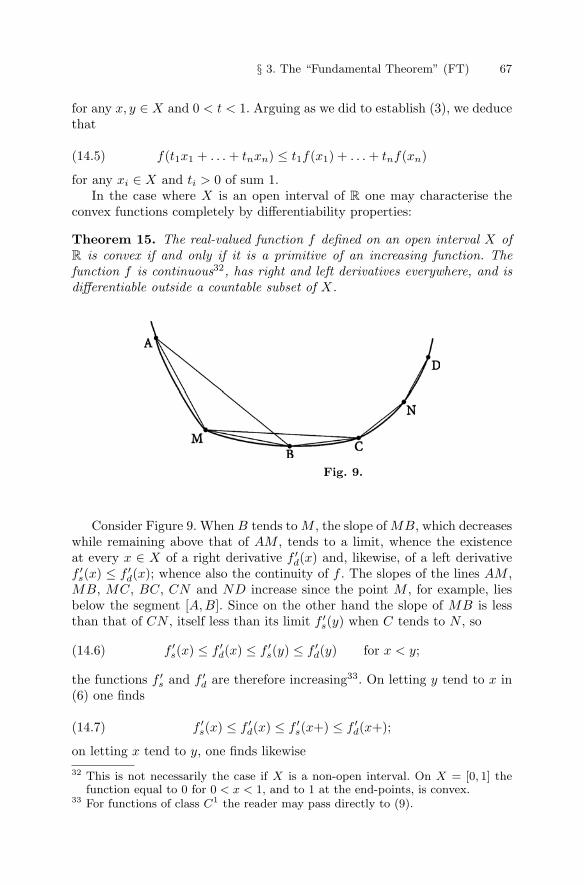
§ 3. The “Fundamental Theorem” (FT) 67
for any x, y ∈ X and 0 < t < 1. Arguing as we did to establish (3), we deducethat
f(t1x1 + . . . + tnxn) ≤ t1f(x1) + . . . + tnf(xn)(14.5)
for any xi ∈ X and ti > 0 of sum 1.In the case where X is an open interval of R one may characterise the
convex functions completely by differentiability properties:
Theorem 15. The real-valued function f defined on an open interval X ofR is convex if and only if it is a primitive of an increasing function. Thefunction f is continuous32, has right and left derivatives everywhere, and isdifferentiable outside a countable subset of X.
Fig. 9.
Consider Figure 9. When B tends to M , the slope of MB, which decreaseswhile remaining above that of AM , tends to a limit, whence the existenceat every x ∈ X of a right derivative f ′
d(x) and, likewise, of a left derivativef ′
s(x) ≤ f ′d(x); whence also the continuity of f . The slopes of the lines AM ,
MB, MC, BC, CN and ND increase since the point M , for example, liesbelow the segment [A,B]. Since on the other hand the slope of MB is lessthan that of CN , itself less than its limit f ′
s(y) when C tends to N , so
f ′s(x) ≤ f ′
d(x) ≤ f ′s(y) ≤ f ′
d(y) for x < y;(14.6)
the functions f ′s and f ′
d are therefore increasing33. On letting y tend to x in(6) one finds
f ′s(x) ≤ f ′
d(x) ≤ f ′s(x+) ≤ f ′
d(x+);(14.7)
on letting x tend to y, one finds likewise32 This is not necessarily the case if X is a non-open interval. On X = [0, 1] the
function equal to 0 for 0 < x < 1, and to 1 at the end-points, is convex.33 For functions of class C1 the reader may pass directly to (9).
68 V – Differential and Integral Calculus
f ′s(y−) ≤ f ′
d(y−) ≤ f ′s(y) ≤ f ′
d(y),
which, applied to x, allows us to complete (7) as
f ′s(x−) ≤ f ′
d(x−) ≤ f ′s(x) ≤ f ′
d(x) ≤ f ′s(x+) ≤ f ′
d(x+).
Now we have f ′d(y) ≤ f ′
s(z) for y < z by (6); on letting y and z tend to x+one finds f ′
d(x+) ≤ f ′s(x+), whence
f ′s(x+) = f ′
d(x+) and likewise f ′s(x−) = f ′
d(x−)
for every x; finally
f ′s(x−) = f ′
d(x−) ≤ f ′s(x) ≤ f ′
d(x) ≤ f ′s(x+) = f ′
d(x+).(14.8)
The functions f ′s and f ′
d being increasing, and so regulated, can be discon-tinuous only on a countable set D of points of X (Chap. III, n◦ 12, Corollaryto Theorem 16 or n◦ 7, Theorem 6 of the present Chap.); (8) shows more-over that the points where they are discontinuous are the same for the twofunctions. Outside D, the six terms of (8) are equal, and f is differentiablesince its right and left derivatives are equal.
The function f being continuous, and admitting, outside D, a derivativeequal, at one’s choice, to the regulated function f ′
s or to f ′d, it must be a
primitive of f ′s and of f ′
d in the sense of n◦ 13; in other words,
f(y) − f(x) =∫ y
x
f ′s(u)du =
∫ y
x
f ′d(u)du
for any x, y ∈ X.Conversely, let us start from an increasing, so regulated, function g on X
and let f be a primitive of g. Consider two points x, y of X and suppose forexample x < y. For t ∈ [0, 1] one has
f [(1 − t)x + ty] − {(1 − t)f(x) + tf(y)} == {f [x + t(y − x)] − f(x)} − t[f(y) − f(x)] =(14.9)
=∫ y−x
0
tg(x + tv)dv − t
∫ y−x
0
g(x + v)dv
as one sees on differentiating the functions f(x+tv) and f(x+v) with respectto v and applying the FT. But since g is increasing, and since v ≥ 0 on theinterval of integration, we have
g(x + tv) ≤ g(x + v) for t ∈ [0, 1].
The difference between the two last integrals is thus ≤ 0 so the function f isconvex, qed.
§ 3. The “Fundamental Theorem” (FT) 69
Corollary 1. A differentiable function f is convex on an open interval if andonly if its derivative is increasing. A twice differentiable function is convexif and only if f ′′(x) ≥ 0 for every x.
For if f ′(x) exists everywhere, and is increasing, so regulated, then f is aprimitive of f ′ and is therefore convex. If f ′ is differentiable it is increasingif and only if f ′′(x) ≥ 0 everywhere, by the mean value theorem (Chap. III,n◦ 16).
The case (a bonus for the reader) of a function f defined on a convexopen subset X of Rp, for example of C, reduces to the preceding ifone assumes f of class C2 on X. In the first place, the convexity of fobviously means that, for any x, y ∈ X, the function t → f [(1−t)x+ty], defined on a convex open subset (i.e. an open interval) of R, isconvex. Since f is of class C1, this function has a derivative equal to
d
dtf [(1−t)x1+ty1, . . . , (1−t)xp+typ] =
∑Dif [(1−t)x+ty](yi−xi)
by the chain rule of Chap. III, n◦ 21. The result obtained is againdifferentiable if f is of class C2, with, for the same reason,
d2
dt2. . . =∑i,j
DjDif [(1 − t)x + ty](yj − xj)(yi − xi).(14.10)
By Corollary 1, this result must be ≥ 0; in particular, we must have(take t = 0) ∑
DjDif(x)uiuj ≥ 0(14.11)
whenever the ui can be put in the form yi − xi for some y ∈ X.But since X is open these differences can, for x given, take all valuessufficiently close to 0, so that, for arbitrary ui ∈ R, (11) must besatisfied by the tui for every t ∈ R sufficiently close to 0; since thissubstitution multiplies (11) by t2 > 0, we conclude that (11) mustbe satisfied for any ui ∈ R: the quadratic form (11) must be positivesemidefinite, as one says in algebra. Conversely, it is clear that if (11)is satisfied for any x ∈ X and ui ∈ R, then the derivative (10) is ≥ 0so long as (1 − t)x + ty ∈ X; the function
t → f [(1 − t)x + ty]
is thus convex, so f is too. Consequently:
Corollary 2. Let f be a real-valued function defined and of class C2
in a convex open set X ⊂ Rp. Then f is convex on X if and only if∑DiDjf(x)uiuj ≥ 0
for any ui ∈ R and x ∈ X.
70 V – Differential and Integral Calculus
Theorem 15 allows us to establish the famous inequalities of Holder andof Minkowski, which are not very useful at our level – but general culture. . . The function ex has an everywhere positive second derivative and so isconvex on R, whence
etx+(1−t)y ≤ tex + (1 − t)ey
for any x, y ∈ R and 0 < t < 1. We can also write this in the form
atb1−t ≤ ta + (1 − t)b(14.12)
for a, b > 0 and even for 0 ≤ a, b ≤ +∞ on agreeing that 0t = 0, (+∞)t =+∞, t.(+∞) = +∞ for t > 0 and that 0.(+∞) = 0.
Now consider an arbitrary set X and suppose that to every function fdefined on X and with values in [0,+∞] one has associated a number µ∗(f)possessing the following properties34:
(IS 1): 0 ≤ µ∗(f) ≤ +∞;(IS 2): the relation f ≤ g implies µ∗(f) ≤ µ∗(g);(IS 3): µ∗(f + g) ≤ µ∗(f) + µ∗(g) for any f, g;(IS 4): µ∗(cf) = cµ∗(f) for every constant c ≥ 0.
If F and G are functions on X with values in [0,+∞] one has
F tG1−t ≤ tF + (1 − t)G
by (12); whence, using (IS 2), (IS 3) and (IS 4),
µ∗(F tG1−t) ≤ µ∗[tF + (1 − t)G] ≤ µ∗(tF ) + µ∗[(1 − t)G]≤ tµ∗(F ) + (1 − t)µ∗(G)
for 0 < t < 1. In particular we see that
µ∗(F ) = µ∗(G) = 1 =⇒ µ∗(F tG1−t) ≤ 1.
If one assumes only that µ∗(F ) and µ∗(G) are finite and nonzero, and ifone applies the last result to the functions F/µ∗(F ) and G/µ∗(G), whichis legitimate by (IS 4), the function F tG1−t is divided by the constantµ∗(F )tµ∗(G)1−t, whence, using (IS 4) again,
µ∗(F tG1−t) ≤ µ∗(F )tµ∗(G)1−t.(14.13)
Now put
34 These conditions generalise the properties of the upper integral established inn◦ 11 and are met in the general theory of integration. It is not really necessaryto assume that µ∗(f) is defined for every positive function on X; it is enoughthat the formulae that we are going to write should be meaningful.
§ 3. The “Fundamental Theorem” (FT) 71
Np(f) = µ∗ (|f |p)1/p ≤ +∞(14.14)
for every function f with complex values on X and every real number p > 0.If f and g are two such functions and if p and q are real numbers > 0, let uschoose F = |f |p, G = |g|q and t = r/p, 1 − t = r/q where r > 0 is such thatr/p + r/q = 1, i.e. such that
1/p + 1/q = 1/r.(14.15)
Then F tG1−t = |f |pr/p|g|qr/q = |fg|r, so that (13) becomes
µ∗(|fg|r) ≤ µ∗ (|f |p)r/pµ∗ (|g|q)r/q
,
whence, on raising both sides to the power 1/r,
Nr(fg) ≤ Np(f)Nq(g) for 1/p + 1/q = 1/r.(14.16)
Note that Nr(f) is finite if Np(f) and Nq(g) are finite because (12), appliedto F = |f |p, G = |g|q, t = r/p, 1 − t = r/q, shows that
|fg|r/r ≤ |f |p/p + |g|q/q,(14.17)
so that it remains to apply the axioms (IS).(16) is the inequality of (Otto) Holder, most often used only for r = 1:
µ∗(|fg|) ≤ µ∗ (|f |p)1/pµ∗ (|g|q)1/q = Np(f)Nq(g);(14.18)
this inequality assumes that 1/p + 1/q = 1 and thus p, q > 1 (conjugateindices). The case where p = q = 2 is just the Cauchy-Schwarz inequalityextended to the functions µ∗.
From (18) one may deduce the inequality
Np(f + g) ≤ Np(f) + Np(g) for p > 1(14.19)
of (Hermann) Minkowski, one of Einstein’s professors at the Polytechnic ofZurich, and, at Gottingen in 1907–1908, the inventor of the interpretationof Relativity in R4 endowed with the quadratic form x2 + y2 + z2 − c2t2.He would probably have gone much further if he had not died soon after . . .There is nothing to prove if the right hand side is infinite or if the left handside is zero. If the right hand side is finite, so too is the left hand side, for,the function xp being convex in x ≥ 0 for p > 1, one has( |f | + |g|
2
)p
≤ 12
(|f |p + |g|p) .
This done, we write
|f + g|p ≤ (|f | + |g|)p = |f |.|f + g|p−1 + |g|.|f + g|p−1.
72 V – Differential and Integral Calculus
Since |f + g|(p−1)q = |f + g|p, we have Nq(|f + g|p−1) < +∞; Holder’sinequality (18) then shows that
µ∗(|f + g|p) ≤ [Np(f) + Np(g)]Nq(|f + g|p−1)
= [Np(f) + Np(g)].µ∗(|f + g|(p−1)q
)1/q
= [Np(f) + Np(g)].µ∗(|f + g|p)1−1/p;
on multiplying both sides by µ∗ (|f + g|p)−1+1/p we obtain
µ∗(|f + g|p)1/p ≤ Np(f) + Np(g),
i.e. (19).
It is probable that the reader has not truly understood these proofs; hemay console himself in knowing that the majority of the professionals are inthe same state, having only checked the argument step-by-step, registeredthe results, and forgotten the proofs for the rest of their lives (unless needingto expound them to students . . .).
Example 1. If f and g are regulated functions on a bounded interval I∣∣∣∣∫
I
f(x)g(x)dx
∣∣∣∣ ≤ Np(f)Nq(f), Np(f + g) ≤ Np(f) + Np(g)(14.20)
where one puts
Np(f) =(∫
I
|f(x)|pdx
)1/p
,
the Lp norm of the function f . You might replace the traditional integralm(f) by the expression
µ(f) =∫
|f(x)|µ(x)dx
where µ is a given positive integrable function; it clearly satisfies conditions(IS 1) to (IS 4) above. One thus finds the inequalities (20) where the symboldx is replaced everywhere by µ(x)dx. Without doubt we will be made toobserve that this “generalisation” is illusory since it follows from the classicalcase on replacing f(x) by f(x)µ(x)1/p and g(x) by g(x)µ(x)1/q; precisely.But the objection falls if one defines µ(f) from an arbitrary Radon measure(n◦ 30).
Example 2. Take for X a finite set and µ∗(f) =∑ |f(x)|. One obtains, in
more traditional notation, the original versions of the inequalities:∣∣∣∑xkyk
∣∣∣ ≤ (∑ |xk|p)1/p (∑
|yk|q)1/q
,(14.21)
§ 3. The “Fundamental Theorem” (FT) 73
(∑|xk + yk|p
)1/p
≤(∑
|xk|p)1/p
+(∑
|yk|p)1/p
.(14.22)
Example 3. Like the preceding, but with an infinite set X and, again, µ∗(f) =∑ |f(x)| ≤ +∞ for every function f with positive values. If the series∑ |xn|p
and∑ |yn|q converge then the series
∑xnyn converges absolutely and
∣∣∣∑xnyn
∣∣∣ ≤ (∑ |xn|p)1/p (∑
|yn|q)1/q
.(14.23)
All this assumes p, q > 1 and 1/p + 1/q = 1. The case p = q = 2 is theCauchy-Schwarz inequality for series, which may be proved much more easilyby passing to the limit starting from the case of a finite sum.
74 V – Differential and Integral Calculus
§ 4. Integration by parts
15 – Integration by parts
The chain rule shows that if f and g are two functions of class C1 then fg isa primitive of the function f ′g + fg′; consequently, in Leibniz’ style,∫
[f ′(x)g(x) + f(x)g′(x)]dx = f(x)g(x),
which can be rewritten in the form∫f ′(x)g(x)dx = f(x)g(x) −
∫f(x)g′(x)dx;(15.1)
this relation between primitives can be transformed into a relation betweendefinite integrals:
∫ b
a
f ′(x)g(x)dx = f(x)g(x)∣∣∣∣ba
−∫ b
a
f(x)g′(x)dx.(15.2)
This is the formula for integration by parts, which allows us to calculate verymany elementary integrals. It remains valid when f and g are the primitivesof two regulated functions, since then the function fg is continuous and hasas derivative the regulated function f ′g+fg′ outside a countable set of points,so is a primitive of f ′g + fg′ (Theorem 12 bis).
Example 1. Let us calculate the primitive∫log(x)dx =
∫log(x).1.dx =
∫log(x).(x)′.dx =
= log(x)x −∫
log′(x)xdx = x log x −∫
1dx,
whence ∫log(x)dx = x log x − x.(15.3)
It is not difficult to check that log x is indeed the derivative of x log x − x.
Example 2. We have∫x5exdx =
=∫
x5(ex)′dx = x5ex −∫
(x5)′exdx = x5ex − 5∫
x4exdx =
= x5ex − 5x4ex + 5.4∫
x3exdx =
§ 4. Integration by parts 75
= x5ex − 5x4ex + 5.4x3ex − 5.4.3∫
x2exdx =
= x5ex − 5x4ex + 5.4x3ex − 5.4.3x2ex + 5.4.3.2∫
xexdx =
= x5ex − 5x4ex + 5.4x3ex − 5.4.3x2ex + 5.4.3.2xex − 5.4.3.2.1∫
exdx =
= x5ex − 5x4ex + 5.4x3ex − 5.4.3x2ex + 5.4.3.2xex − 5.4.3.2.1ex.
The reader can generalise this to xnex for n ∈ N.And for n < 0? Let’s try our luck.∫
x−2exdx =
=∫
(−x−1)′exdx = −ex/x +∫
x−1exdx =
= −ex/x +∫
log′(x)exdx = −ex/x + ex log x −∫
ex log(x)dx =
= −ex/x + ex log x −∫
ex[x log(x) − x]′dx =
= −ex/x + ex log x − ex[x log(x) − x] +∫
ex[x log(x) − x]dx,
and you may continue indefinitely without ever managing to eliminate thefunction ex log x. It would certainly be enough to know one primitive, whichthe theory of the power series allows us to find theoretically; but in practiceone naturally tries to express the given integral in terms of a simple combi-nation of “elementary”, i.e. already known, functions. This is impossible forthe functions xsex with s /∈ N, or ex log x, or exp(exp(x)), etc.
Moral: one does not have to go very far to find oneself face to face withelementary functions whose primitives are not elementary. To be able to cal-culate a primitive explicitly is almost always a miracle, and even, in teachinganalysis, a contrived miracle: the calculation put to you as an exercise is fea-sible because the author of the exercise knows it in advance, generally fromhaving read through the older authors to extract some from the very manyexercises of the same kind.
In fact, mathematicians who have sought in vain to calculate a primitiveor a definite integral of a function which is important to their applications – ashappens often in mechanics or in physics – always end up changing their tac-tics: they give a name once and for all to the mysterious primitive or integralin question, and, instead of calculating it, try to establish its useful proper-ties (differential equation, series expansions, asymptotic behaviour, integralslinked to these functions, etc.); these are the special functions. At the lowestlevel, this is what has always been done for the trigonometric functions: onegives them a name, and, instead of calculating them from beautiful simplealgebraic formulae which do not exist, one derives their properties. This is
76 V – Differential and Integral Calculus
also what the theory of the elliptic functions has allowed mathematiciansto do for the primitives of the functions of the form P (x)1/2, where P is apolynomial of degree 3 or 4.
Example 3. Let us try to calculate the functions
In =∫
xn cos x.dx, Jn =∫
xn sin x.dx.(15.4)
We may write
In =∫
xn sin′ x.dx = xn sin x − n
∫xn−1 sin x.dx
and continue. It is more economical to observe that
In + iJn =∫
xneixdx
and to calculate as in Example 2 or, for good measure, to calculate∫
xnetxdxfor every t ∈ C. We find easily∫
xnetxdx =(15.5)
= etx[xn/t − nxn−1/t2 + n(n − 1)xn−2/t3 + . . . + (−1)nn!/tn+1
],
whence, for t = i, on separating the real and imaginary parts,
In = xn sin x + nxn−1 cos x − n(n − 1)xn−2 sin x −(15.6’)− n(n − 1)(n − 2)xn−3 cos x + . . . ,
Jn = −xn cos x + nxn−1 sin x + n(n − 1)xn−2 cos x −(15.6”)− n(n − 1)(n − 2)xn−3 sin x − . . . .
Example 4. Put log2 x = (log x)2 and calculate∫x. log2 x.dx =
∫ (12x2
)′log2 x.dx =
12x2 log2 x − 1
2
∫x2(log2 x)′dx =
=12x2 log2 x − 1
2
∫x22 log x(log′ x)dx =
=12x2 log2 x −
∫x. log x.dx =
=12x2 log2 x − 1
2x2 log x +
12
∫x2 log′ x.dx =
=12x2 log2 x − 1
2x2 log x +
12
∫xdx =
=12x2 log2 x − 1
2x2 log x + x2/4.
One should not forget that an arbitrary constant may be added to the resultin all these formulae.
§ 4. Integration by parts 77
16 – The square wave Fourier series
We are now in a position to justify the square wave series [Chap. III, eqn. (2.4)and n◦ 11, Example 1]
s(x) = cos x − cos 3x/3 + cos 5x/5 − . . . = π/4 for |x| < π/2(16.1)
which Fourier first obtained by breathtaking meaningless calculations; itsvalue for π/2 < |x| < π, namely −π/4, follows from (1) on replacing x byπ − x. Fourier himself did not mention this explicitly in his memoir, but onehas to believe that he had some doubts since he later felt the need to justifyhis result by patently more reasonable methods. We shall follow him.
We start quite naturally by calculating the partial sum
sn(x) = cos x − cos 3x/3 + . . . + (−1)n−1 cos(2n − 1)x/(2n − 1),(16.2)
not by an impossible direct calculation, but by differentiating it. We have
s′n(x) = − sin x + sin 3x − . . . + (−1)n sin(2n − 1)x,
whence, putting q = eix and using Euler’s formulae,
−2is′n(x) =(q − q−1
)− (q3 − q−3)
+ . . . + (−1)n−1(q2n−1 − q−2n+1
)=
= q[1 − q2 + . . . + (−1)n−1q2n−2
]− q−1[1 − q−2 + . . .
]=
= q1 − (−1)nq2n
1 + q2− q−1 1 − (−1)nq−2n
1 + q−2=
=1 − (−1)nq2n
q−1 + q− 1 − (−1)nq−2n
q + q−1=
= (−1)n+1 q2n − q−2n
q + q−1= (−1)n+12i sin 2nx/2 cos x.
Thuss′n(x) = (−1)n sin 2nx
2 cos x.
This calculation assumes cos x �= 0, which is the case in the interval of inter-est.
From this we deduce, by the FT, that
sn(y) − sn(x) = (−1)n
∫ y
x
sin 2nt
2 cos tdt(16.3)
for x and y in the open interval I =]− π/2, π/2[. Since the sum of the seriesis supposed to be a constant function we ought to show that the difference(3), which tends to s(y) − s(x), tends to 0 as n increases indefinitely.
This is not obvious at first sight, but let us integrate by parts; we get∫ y
x
sin 2nt
cos tdt =
− cos 2nt
2n. cos t
∣∣∣∣yx
− 12n
∫ y
x
cos 2ntsin t
cos2 tdt.
78 V – Differential and Integral Calculus
As n increases indefinitely the first term of the right hand side tends to 0because of the factor n in the denominator. Likewise for the second term,for, in the interval of integration, we have
| cos 2nt. sin t| ≤ 1, cos2 t ≥ m
where m is the minimum of cos2 t between x and y; it is > 0 because acontinuous function attains its minimum on a compact interval, and theinterval [x, y] contains no odd multiple of π/2. The factor 1/2n thereforeprovides an upper bound O(1/n).
The sum s(x) of the series (1) is therefore constant on the interval|x| < π/2. Its value must be
s(0) = 1 − 1/3 + 1/5 − . . . = π/4,(16.4)
Leibniz’ series.We proved (4), more or less, in Chap. IV, n◦ 14 using the series expansion
arctan y = y − y3/3 + y5/5 − . . . ;(16.5)
one obtains this by starting from the formula
arctan′ y = 1/(1 + y2) = 1 − y2 + y4 − . . .
and applying the method valid for every power series. Nevertheless one mustbe aware of the fact that this applies to the interior of the disc of convergence,i.e. for |y| < 1; now Leibniz’ formula corresponds precisely to the value y = 1,where arctan y = π/4. To justify this one has to argue as we did a propos theseries log(1+x), which, for x = 1, yields the series log 2 = 1−1/2+1/3− . . .by passage to the limit: for 0 ≤ y ≤ 1 the series (5) is alternating and hasdecreasing terms, the difference between its total sum and its n-th partialsum is thus majorised by its n-th term, so by 1/(2n + 1) for any y, whenceone concludes that the partial sums of (5) converge to the total sum uni-formly on the closed interval [0, 1]. The total sum of the series is thereforea continuous function there; likewise for the function arctan y; now, if twofunctions are continuous for y ≤ 1, and coincide for y < 1, then they remainequal at y = 1. Whence (4).
Starting from the series (1), one may obtain others by integration. Cal-culating formally,∫ x
0
s(t)dt = sin x − sin 3x/32 + sin 5x/52 − . . .(16.6)
and since s(t) is a step function, it will not be difficult to calculate the integraldirectly. But first one has to justify integrating the series (1) term-by-term.
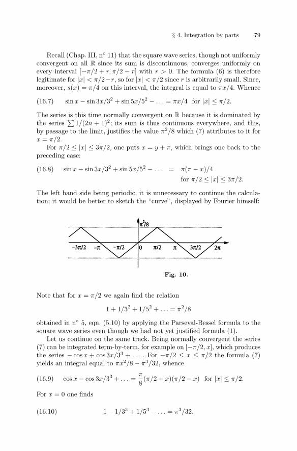
§ 4. Integration by parts 79
Recall (Chap. III, n◦ 11) that the square wave series, though not uniformlyconvergent on all R since its sum is discontinuous, converges uniformly onevery interval [−π/2 + r, π/2 − r] with r > 0. The formula (6) is thereforelegitimate for |x| < π/2−r, so for |x| < π/2 since r is arbitrarily small. Since,moreover, s(x) = π/4 on this interval, the integral is equal to πx/4. Whence
sin x − sin 3x/32 + sin 5x/52 − . . . = πx/4 for |x| ≤ π/2.(16.7)
The series is this time normally convergent on R because it is dominated bythe series
∑1/(2n + 1)2; its sum is thus continuous everywhere, and this,
by passage to the limit, justifies the value π2/8 which (7) attributes to it forx = π/2.
For π/2 ≤ |x| ≤ 3π/2, one puts x = y + π, which brings one back to thepreceding case:
sin x − sin 3x/32 + sin 5x/52 − . . . = π(π − x)/4(16.8)for π/2 ≤ |x| ≤ 3π/2.
The left hand side being periodic, it is unnecessary to continue the calcula-tion; it would be better to sketch the “curve”, displayed by Fourier himself:
Fig. 10.
Note that for x = π/2 we again find the relation
1 + 1/32 + 1/52 + . . . = π2/8
obtained in n◦ 5, eqn. (5.10) by applying the Parseval-Bessel formula to thesquare wave series even though we had not yet justified formula (1).
Let us continue on the same track. Being normally convergent the series(7) can be integrated term-by-term, for example on [−π/2, x], which producesthe series − cos x + cos 3x/33 + . . . . For −π/2 ≤ x ≤ π/2 the formula (7)yields an integral equal to πx2/8 − π3/32, whence
cos x − cos 3x/33 + . . . =π
8(π/2 + x)(π/2 − x) for |x| ≤ π/2.(16.9)
For x = 0 one finds
1 − 1/33 + 1/53 − . . . = π3/32.(16.10)
80 V – Differential and Integral Calculus
On continuing to integrate the reader would find infinitely many otherformulae of the same kind, the first already in Euler, by other methods, ofcourse. One may also examine what the Parseval-Bessel formula of (5.6) or(5.7) of this Chap. V may provide; there is no problem since the successiveprimitive series of the square wave series are (more and more) absolutelyconvergent. This kind of exercise is appreciably more instructive than calcu-lating a primitive of a rational fraction chosen only to make the candidatestumble over calculations of no other interest.
17 – Wallis’ formula
Let us put
In =∫ π/2
0
sinn x.dx(17.1)
for n ∈ N. First,
I0 = π/2, I1 = 1.(17.2)
Next, integrate by parts, whence
In = −∫ π/2
0
sinn−1 x. cos′ x.dx =
= − sinn−1 x. cos x∣∣π/2
0+∫ π/2
0
(sinn−1 x)′ cos x.dx =
= (n − 1)∫ π/2
0
sinn−2 x. cos2 x.dx = (n − 1)(In−2 − In).
Finally we obtain In = In−2(n − 1)/n, whence
I2n =(2n − 1)(2n − 3) . . . 1
2n(2n − 2) . . . 2I0 with I0 = π/2
and
I2n+1 =2n(2n − 2) . . . 2
(2n + 1)(2n − 1) . . . 3I1 with I1 = 1.
Since 0 ≤ sin x ≤ 1 on the interval of integration it is clear that In+1 ≤ In,thus that I2n+1 ≤ I2n ≤ I2n−1, whence
1 ≤ I2n/I2n+1 ≤ I2n−1/I2n+1 = 1 + 1/2n.
The ratio
I2n/I2n+1 =(2n + 1)(2n − 1)2(2n − 3)2 . . . 32
(2n)2(2n − 2)2 . . . 22
π
2
thus tends to 1, whence Wallis’ famous formula
§ 4. Integration by parts 81
2π
= lim1.3.3.5.5.7 . . . (2n − 1)(2n + 1)
2.2.4.4.6.6 . . . 2n.2n.(17.3)
Fourier, who used it, wrote it in the form
2π
= 3.3.5.5.7.7..../2.2.4.4.6.6....;
though neither the numerator nor the denominator makes any sense, onemay try to interpret it as an infinite product (Chap. IV, n◦ 17). In the form3/2.3/2.5/4.5/4 . . . it is clearly divergent since the general term is of the form(p + 1)/p = 1 + 1/p. One may then try the product of all the expressions3.3/2.2, etc., i.e. the infinite product with general term (2n + 1)2/4n2 =(1 + 1/2n)2; but
(1 + 1/2n)2 = 1 + 1/n + 1/4n2 = 1 + un
where the series∑
un is divergent since un ∼ 1/n; new catastrophe. Onemight prefer the groupings 3.3/4.4, etc., which leads to the product of the
(2n+1)2/(2n+2)2 = [1 − 1/(2n + 2)]2 = 1−1/(n+1)+1/4(n+1)2 = 1+un,
which diverges as much as the preceding ones, and for the same reason,namely that un ∼ −1/n. The solution is to write (3) in the form
2/π = lim1.32.2
3.54.4
5.76.6
. . .(2n − 1)(2n + 1)
2n.2n,
or
2/π =∞∏
n=1
(1 − 1/4n2) = (1 − 1/4)(1 − 1/16)(1 − 1/36) . . .(17.4)
The infinite product is this time absolutely convergent like the series∑
1/n2
and is greatly preferable to the formula (3), which would lead you to perditionas we have just seen.
A very fast proof Wallis’ formula comes from starting from the infiniteproduct
sin πx = πx∏
(1 − x2/n2);
one recovers Wallis when x = 1/2.
82 V – Differential and Integral Calculus
§ 5. Taylor’s Formula
18 – Taylor’s Formula
Chap. II, n◦ 19, has shown us that if a function f(z) is analytic on an openset in C containing a point a, then the power series which represents it on aneighbourhood of a has the form
f(z) = f(a) + f ′(a)(z − a)/1! + f ′′(a)(z − a)2/2! + . . . .(18.1)
This result applies in particular to functions which are defined and analyticon an interval in R.
One obviously cannot hope for so much for every function defined on suchan interval, even if it is indefinitely differentiable, since all the derivatives ofsuch a function may well be zero at a without the function being zero on aneighbourhood of a, as Cauchy showed (Chap. IV, end of n◦ 5). The situationis still more desperate when we deal with functions which are not indefinitelydifferentiable.
But let us start from the formula
f(t)∣∣∣xa
=∫ x
a
f ′(t)dt =∫ x
a
f ′(t)P0(t)dt
where P0(t) = 1, and let P1(t) be a primitive of P0. An integration by partsshows that
f(t)∣∣∣xa
= f ′(t)P1(t)∣∣∣xa−∫ x
a
f ′′(t)P1(t)dt.
If P2(t) is a primitive of P1 and if one integrates again by parts, one finds
f(t)∣∣∣xa
= f ′(t)P1(t) − f ′′(t)P2(t)∣∣∣xa
+∫ x
a
f ′′′(t)P2(t)dt.
If f is of class Cn+1, i.e. has continuous derivatives of order ≤ n + 1 onthe interval I of R where it is defined, one may continue up to the integralinvolving f (n+1). The result is clearly that, if one chooses polynomials Pk(t)satisfying
P ′k = Pk−1, P0 = 1,(18.2)
then
f(t)∣∣∣xa
= f ′(t)P1(t) − f ′′(t)P2(t) + . . . + (−1)n−1f (n)(t)Pn(t)∣∣∣xa
+
+ (−1)n
∫ x
a
f (n+1)(t)Pn(t)dt.(18.3)
Since we would like to express f(x) in terms of its derivatives at a and ofthe factors (x − a)k, we ought to choose the Pk so as to make the terms
§ 5. Taylor’s Formula 83
f ′(x), . . . , f (n)(x) that appear in the integrated parts disappear from theright hand side of (3); to do this we have to choose the Pk to vanish fort = x, in other words
Pk(t) = (t − x)k/k! = (t − x)[k].(18.4)
After this calculation we obtain the following result:
Theorem 16. Let f be a function defined and of class Cn+1 on an intervalI of R. Then, for any a, x ∈ I,
f(x) = f(a) + f ′(a)(x − a) + f ′′(a)(x − a)[2] + . . .(18.5). . . + f (n)(a)(x − a)[n] + rn(x)
where
rn(x) =∫ x
a
f (n+1)(t)(x − t)[n]dt.(18.6)
This is Taylor’s formula with integral remainder for functions of class Cn+1,and is due, with this very proof, to Cauchy.
An expression for the remainder that is sometimes more useful comesfrom putting x = a + h and replacing the function f(x) by the functiong(u) = f(a + uh), where u now varies in [0, 1]. The limits a and x become 0and 1 and we have g(p)(u) = hpf (p)(a + uh) by the most trivial form of thechain rule. On applying the formula to g between u = 0 and u = 1 one findsthe following version of Taylor’s formula for f :
f(a + h) = f(a) + f ′(a)h + . . . + f (n)(a)hn/n! + rn(a + h),(18.5’)
where
rn(a + h) =hn+1
n!
∫ 1
0
f (n+1)(a + uh)(1 − u)ndu.(18.6’)
The simplest and most useful particular case is
f(x + h) − f(x) − f ′(x)h =12h2
∫ 1
0
f ′′(x + uh)(1 − u) du.(18.6”)
For a = 0, (5) becomes a formula of Maclaurin type:
f(x) = f(0) + f ′(0)x + f ′′(0)x2/2! + . . . + f (n)(0)xn/n! + rn(x)(18.7)
with
rn(x) =∫ x
0
f (n+1)(t)(x − t)[n]dt =(18.8)
=xn+1
n!
∫ 1
0
f (n+1)(ux)(1 − u)ndt.
84 V – Differential and Integral Calculus
This expresses f as the sum of a polynomial
p(x) = f(0) + f ′(0)x + . . . + f (n)(0)x[n]
of degree n having at x = 0 (or, in the general case, at x = a) the samederivatives of order ≤ n as f , and a “remainder” given by (8). It is called the“remainder” because, if f is analytic, rn(x) is actually the n-th remainder ofthe Taylor series of f ; but here there is no series. Moreover, when one speaksof the partial sums and of the remainders of a series, one very much hopesthat these will be increasingly negligible as n increases.
The true situation is less impressive. If you apply (7) to an indefinitelydifferentiable function all of whose derivatives are zero at the origin, you willfind f(x) = rn(x). Far from being negligible, the “remainder” is then thepredominant term.
All the same, one can estimate it. Since f (n+1) is continuous it is boundedon every compact set contained in the interval I where f is defined. If thenx remains in a compact interval K contained in I and containing a (forexample, an interval of centre a if a is interior to I), and if, as always, oneputs ∥∥f (p)
∥∥K
= supx∈K
∣∣f (p)(x)∣∣,(18.9)
then∣∣f (n+1)(t)(x − t)n
∣∣ ≤ ∥∥f (n+1)∥∥
K. |(x − t)n| on the interval of integra-
tion; but on this interval we have |(x − t)n| = ±(x − t)n with the + sign ifx > a and the − sign if x < a, in which case the + sign is reestablished fromthe fact that the oriented integral from a to x is accounted negatively. Thefunction t → (x − t)[n] having as a primitive the function
t → −(x − t)[n+1]
which vanishes for t = x, one finds finally that
|rn(x)| ≤ ∥∥f (n+1)∥∥
K.|x − a|n+1/(n + 1)! for x ∈ K.(18.10)
(6) makes the result even more obvious.Modifying the notation, in particular we have
f(a + h) = f(a) + f ′(a)h + f ′′(a)h[2] + . . .(18.11). . . + f (n)(a)h[n] + O(hn+1)
as h tends to 0. If, for example, a function f of class C∞ vanishes togetherwith all its successive derivatives at x = a, then
f(x) = O((x − a)n
)for every n
as x tends to a, which shows that, even in this case, Taylor’s formula doesprovide information: f(a+h) tends to 0 more rapidly than every power of h.
§ 5. Taylor’s Formula 85
We say then that the function f is flat at the point a. The aeroplane whichwill never be built follows a trajectory of this kind on landing.
Exercise. Prove that
p(h) = f(a) + f ′(a)h + . . . + f (n)(a)h[n]
is the only polynomial satisfying
f(a + h) = p(a) + o(hn), d◦(p) ≤ n.
These results assume that f (n+1) exists and is continuous. One can infact prove the formula otherwise, without this last hypothesis, in the caseof a real-valued function; the practical usefulness of the result in relation tothe preceding one is weak, to speak moderately, but the proof is ingenious.To simplify we restrict to the Maclaurin case, and, for x = b given, let usconsider the functions
g(t) = f(b) − f(t) − f ′(t)(b − t) − . . . − f (n)(t)(b − t)[n],
h(t) = g(t) − g(0)(b − t)[n+1]/b[n+1]
like Cauchy and his uniformed students, most of whom were probably doz-ing. By hypothesis, g, and so h also, have first derivatives, not necessarilycontinuous, between 0 and b. We have h(0) = 0 by a direct calculation, andh(b) = g(b) = f(b) − f(b) = 0. Therefore there is a number ξ between 0 andb where h′(ξ) = 0 (mean value theorem, or even Rolle’s theorem, Chap. III,n◦ 16). Now a calculation similar to the one that led us to (3) shows that
g′(t) = −f (n+1)(t)(b − t)[n],
whence
h′(t) = −f (n+1)(t)(b − t)[n] + g(0)(b − t)[n]/b[n+1]
=[g(0) − f (n+1)(t)b[n+1]
](b − t)[n]/b[n+1].
Since h′(ξ) = 0 we therefore have g(0) = f (n+1)(ξ)b[n+1] for a ξ between 0and b = x, and since
g(0) = f(x) −{
f(0) + f ′(0)x + . . . + f (n)(0)x[n]}
,
finally we have
f(x) = f(0) + f ′(0)x + . . . + f (n)(0)x[n] + f (n+1)(ξ)x[n+1];(18.12)
this is Maclaurin’s formula with Lagrange remainder. In the general case oneobtains
86 V – Differential and Integral Calculus
f(a + h) = f(a) + f ′(a)h + f ′′(a)h[2] + . . .(18.13). . . + f (n)(a)h[n] + f (n+1)(a + θh)h[n+1]
where, yet again, f has real values, is (n + 1) times differentiable, and wherethe number traditionally denoted by θ is between 0 and 1 so that the pointξ = a + θh lies between a and x = a + h.
Applied to a function of class C∞ these results sometimes allow us topass to a Taylor series.
Example 1. Take a = 0 and f(x) = sinx. For n = 2p one finds |rn(x)| ≤|x|2p/(2p)! since the successive derivatives are everywhere less than 1 in mod-ulus. On passing to the limit one thus recovers the formula
sin x = lim[x − x3/3! + . . . + (−1)p−1x2p−1/(2p − 1)!
].
This argument can be generalised. For a C∞ function the Taylor formulawith remainder applies for any n. To pass from this to a power series expan-sion, it suffices – but this is the crucial point – to know that the remaindertends to 0 as n increases indefinitely, in other words to have a suitable es-timate of the successive derivatives. If for example there exist constants Mand q such that |f (n)(x)| ≤ Mqn for any n, then the formula (10), for a = 0,shows that
|rn(x)| ≤ Mqn|x|n/n! = M(q|x|)n/n!
and the passage to the limit is justified. In other cases one has to argue insome other way.
Example 2. Take f(x) = ex. All the derivatives are equal to f , so that, for Kgiven, the factor
∥∥f (n+1)∥∥
Kin (10) does not depend on n. Thus lim rn(x) = 0
for every x and one recovers the power series for the exponential function.
Example 3. Take f(x) = (1 + x)s with s ∈ C and −1 < x, whence
f (n+1)(x) = s(s − 1) . . . (s − n)(1 + x)s−n−1.
Here, by (8),
rn(x) = s(s − 1) . . . (s − n)xn+1
n!
∫ 1
0
(1 + ux)s−n−1(1 − u)ndt,
or
rn(x) =s(s − 1) . . . (s − n)
n!xn+1
∫ 1
0
(1 + xu)s−1
(1 − u
1 + xu
)n
du.
For x > −1 we have 1 + xu > 1 − u on the interval of integration, so that0 < (1 − u)n/(1 + xu)n < 1 for every n. The modulus of the integral istherefore less than a number independent of n. Since the series with general
§ 5. Taylor’s Formula 87
term s(s − 1) . . . (s − n)xn+1/n! converges for |x| < 1 (use the un+1/un
criterion, this is not exactly the binomial series), its general term tends to 0.Likewise therefore for rn(x). On passing to the limit in Taylor’s formula oforder n one thus recovers Newton’s series
(1 + x)s = 1 + sx + s(s − 1)x2/2! + . . .
for |x| < 1, x real, s complex.
We said above that if f is of class Cn+1 then the remainder in the Taylorformula is O
((x − a)n+1
))as x tends to a. One may improve this result for
f real, assuming f (n+1)(a) �= 0. The ratio rn(x)/(x − a)n+1 = f (n+1)(ξ) thentends to f (n+1)(a) since the derivative of order n + 1 is continuous and ξ liesbetween a and x, so tends to a. If one assumes f (n+1)(a) �= 0, then, in theMaclaurin case, for simplicity,
f(x) − f(0) − f ′(0)x − . . . − f (n)(0)x[n] ∼ f (n+1)(0)x[n+1](18.14)
as x tends to 0, the ∼ sign signifying, we recall, that the ratio between thetwo sides of (14) tends to 1.
This formula sometimes allows one to calculate the limits of quotientsf(x)/g(x) as x tends to a point a where f(a) = g(a) = 0. For f and g ofclass Cn, suppose that we have
f(a) = f ′(a) = . . . = f (n−1)(a) = 0,g(a) = g′(a) = . . . = g(n−1)(a) = 0, g(n)(a) �= 0.
On a neighbourhood of a one has g(x) ∼ g(n)(a)(x − a)[n]. If f (n)(a) �= 0,then likewise f(x) ∼ f (n)(a)(x − a)[n]. Consequently
lim f(x)/g(x) = f (n)(a)/g(n)(a).(18.15)
If f (n)(a) = 0 then f(x) = o ((x − a)n) and the result remains valid. Forexample, to find the limit of the ratio
tan x − x
x − sin x
as x tends to 0. Here f(0) = f ′(0) = f ′′(0) = 0, f ′′′(0) = 2 andg(0) = g′(0) = g′′(0) = 0, g′′′(0) = 1. The limit is therefore 1/2.
This is the famous l’Hopital’s rule (he proved it for n = 1, the generalcase being apparently due to Maclaurin), named for a Parisian marquis who,in 1696, earned himself an enviable mathematical reputation by publishinga book entitled Analyse des infiniment petits, pour l’intelligence des lignescourbes, the first exposition to the public of what one then knew as thedifferential calculus chez Leibniz and the Bernoullis. The author made nomystery of the fact that he had learned everything from his correspondence
88 V – Differential and Integral Calculus
and conversations with them: “I have simply appropriated their discoveriesand those of Mr. Leibnis [sic]”, he wrote, skimping the name of his hero,not even giving him a francophone t. This did not prevent Johann Bernoullifrom accusing him of having plagiarised one of his manuscripts and fromattacking him in 1742, which was 38 years after the death of the presumedculprit. Since Johann and Jakob Bernoulli did not hesitate to accuse eachother of plagiarism in the years from 1695, it is probably better to reserveone’s judgement, as does Moritz Cantor, pp. 222–228 of his Vol. III.
“Science is a cruel game. One shoots one’s adversaries down in flames,one grills one’s competitors, one demolishes one’s rivals”, Loup Verlet tells us,p. 97 of La malle de Newton. One should not disdain disputes over priority;they reveal one of the most permanent and pervasive traits of the psychologyof scientists: the defence of their intellectual property. They are an obligatorycorollary of the following principle: the second person to prove a theorem orto discover an AIDS vaccine will not enhance his reputation; he has lost histime, except insofar as the necessary work may have taught him techniquesof future application. One has to be the first35. Moreover, since scientists,and particularly “pure” mathematicians, derive no capital from their workother than the recognition of their prowess by their peers36, those who valuethis have no choice. Those who patent their discoveries – again not the caseof the pure mathematicians, except recently in cryptology37 – or depend on35 The subject is expounded with raw clarity in an interview with a Franco-
American biologist, Portrait of a biologist as capitalist savage, to be found inBruno Latour, Petites lecons de sociologie des sciences (Paris, La Decouverte,1993). The subject had inspired Robert K. Merton much earlier. In the real worldit happens that a new result is obtained almost simultaneously by researchersworking independently of one another; questions of priority are of more interestto them than to spectators. A particularly extreme case is described by NicholasWade, The Nobel Duel (Doubleday, 1981). In an other domain, let us quotethe immortal declaration of the heroic Frenchman, who, on account of a youngGerman, missed first place in the cyclists’ Tour de France of 1997: “What ismissing, I think, is the opportunity to chance on a year without someone betterthan oneself.”
36 This is the function of prizes, medals of gold or of chocolate, colloquia in honourof, seats in academies, etc. which scientists dish out for mutual reward andadmiration. In mathematics, it has even happened, over the last fifteen years,that the complete works of great men have been published before their deaths,despite having to add supplementary volumes later. This facilitates colleagues’work, but the psychological effect on the person so honoured is probably notnegligible. The Science Citation Index, moreover, allows every scientist to knowhow many times his papers have been cited each year. When the total exceeds ahundred (for Einstein, the record holder, the total even exceeded nine hundredsome years ago), one might think that the “reward” is sufficient.
37 Neal Koblitz, A Course in Number Theory and Cryptography (Springer, 2d. ed.,1994), propounds the hypothesis that publications in certain parts of numbertheory may some day have to be submitted to preliminary censoring by theNational Security Agency. This idea is not so wild, since, when the public keysystems invented by mathematicians – their own enterprise – appeared some
§ 5. Taylor’s Formula 89
subventions from organisations advised by scientists have no more: if thehormone you are trying to synthesise may bring you fifty thousand dollars ayear for seventeen years it is urgent not to be second.
With the passion for their profession, which, throughout history, has ledscientists – not all, of course – to accept unworthy or mediocre conditions oflife or work, this is the reason why you will see first class people spend sixtyhours per week in the laboratory, for forty years, for a CNRS “director ofresearch” salary, which any Polytechnic student or former pupil of an HauteEcole des Etudes Commerciales Liberales et Avancees can obtain in industryor in a bank two years after leaving the institution. And so one lauds thedisinterestedness of these “heroes of science” who have no choice.
No choice? After all, as a garage owner who presented an unconscionablyoverinflated account explained to the present author (who, scion of the lowermiddle class, was not a customer of great standing and did not care to acceptit), “with your brain, you should have chosen another profession”. Garageowner, for example. The garage owners could, in exchange, write the mathe-matics which sells itself cheap, teach the chemistry of polymers or the historyof the Middle Ages to two hundred students every year, or try to understandAlzheimer’s disease. Then we might praise the disinterestedness of the garageowners.
Others say that the ill-paid scientists are recompensed in that they enjoythemselves; this may often be true while they are working, but their familiesdo not always appreciate this, and the argument does not have a universalvalidity. Marcel Dassault, the famous French aeroplane manufacturer, said,and repeated during his life, that what “amused him”, was to “make aero-planes” and one does not doubt this. This did not stop him from going tohis office in a Rolls Royce, and this did not stop his son, who also amuseshimself as he can and continues to make man-hunting fighter planes, from
dozen years ago, the reactions of the NSA have been (i) to try to forbid them(in France, their use is subject to prior authorisation), (ii) to impose limits onthe degree of security, (iii) to take charge of research contracts in this field.Remember that the NSA, created in 1952 and with an enormous budget, hasthe mission of ensuring the security of the telecommunications of the Americangovernment and the insecurity of those of others; see James Bamford, The PuzzlePalace (Houghton Mifflin, 1982) and Body of Secrets (Arrow Books, 2003). In“militarily sensitive”areas, access to an American thesis, or to certain courses orseminars, may be limited to people who have submitted to a “security clearance”guaranteeing their “loyalty”. In the USSR, all scientific or technical publicationswere, in principle, subject to prior censorship. Koblitz notes that, up to veryrecently, number theory had never lent itself to any application outside puremathematics. The interest of some mathematicians in cryptology is howeverlongstanding – Viete and Wallis for example – and one knows the part playedduring the War by the Turing team; as for those of our contemporaries who areinvolved, they do not have to proclaim it urbi et orbi. The novelty is the recourseto very advanced mathematics, with, necessarily, the cooperation of professionalsin the theory, simply to understand it; the bridge players of the Enigma projectare probably not enough.
90 V – Differential and Integral Calculus
setting himself as the aim of his animal hunting for 1998 to kill, from a tur-reted (armoured?) 4 × 4, one hundred and eighty-five head of large game inhis modest property of eight hundred hectares near Paris, which landed himin trouble38. Mr. Gates, despite his N(t)1010 dollars, also seems to amusehimself.
Another long trivial theme – though not in the XVIIth century for Fer-mat –, the question of the maxima and minima of functions. If a differentiablefunction f has a local maximum or minimum at a point a i.e. if, on a neigh-bourhood of a, one has f(x) ≤ f(a) in the first case and f(x) ≥ f(a) inthe second, it is clear that f ′(a) = 0. But this condition does not suffice,as shown by the function x3 at x = 0. To elucidate the question one has toexamine the higher derivatives. If
f ′(a) = f ′′(a) = . . . = f (n)(a) = 0, f (n+1)(a) �= 0,
then f(x) − f(a) ∼ f (n+1)(a)(x − a)[n+1] as we have seen; consequently, thedifference f(x) − f(a) has the sign of the right hand side for x sufficientlynear a, whence the conclusion: maximum if n is even and f (n+1)(a) < 0,minimum if n is even and f (n+1)(a) > 0, while the graph of f crosses ahorizontal tangent (point of inflexion) if n is odd.
38 Le Monde of 23 April 1997; the officials of the National Water and Forests Officeapparently do not appreciate that the methods honoured in military aviationsince the Great War are being applied to deer and boar.
§ 6. The change of variable formula 91
§ 6. The change of variable formula
19 – Change of variable in an integral
As we said above, the rules for calculating derivatives can be interpretedin the language of integrals. We have seen the interpretation of the rela-tion (fg)′ = f ′g + fg′ in terms of primitives. The other fundamental ruleof calculus, namely that the derivative of a composite function f [u(x)] isf ′[u(x)].u′(x), likewise leads to an almost trivial integral formula, but it fa-cilitates many explicit evaluations. It also has very important applications,mainly in the theory of line integrals (Vol. III).
Theorem 17. Let u be a real function defined and of class C1 on a compactinterval I = [a, b], and f a function defined and continuous on the intervalJ = u(I). Then ∫ u(b)
u(a)
f(y)dy =∫ b
a
f [u(x)]u′(x)dx.(19.1)
For, let F be a primitive of f on J , so that the left hand side is equal toF [u(b)] − F [u(a)]. The function G(x) = F [u(x)] is differentiable on I andG′(x) = F ′[u(x)]u′(x) = f [u(x)]u′(x). The right hand side of (1) is thusequal to G(b) − G(a) = F [u(b)] − F [u(a)], i.e. to the left hand side, qed.
Note that we are dealing with oriented integrals in this formula, since,even if a < b, one may well have u(a) > u(b).
In the Leibniz notation for primitives one would write∫f(y)dy =
∫f ′[u(x)]u′(x)dx.(19.2)
The formula is self-explanatory: one replaces y by its expression as a functionof x, simultaneously in f(y) and in dy (Chap. III, n◦ 14 and 15). This isone of the great advantages of Leibniz’ system, with the analogous formulady/dx = dy/du.du/dx.
One may widen the hypotheses of Theorem 17 a little when applying itto regulated functions, but the reader new to the subject would be better tokeep to the very simple Theorem 17 for the moment.
The whole question is to reassure oneself that, F being a primitive ofthe regulated function f and u a primitive of the regulated function u′ inthe sense of n◦ 13, then G(x) = F [u(x)] is again a primitive of f [u(x)]u′(x).Since G is continuous, because u and F are, it is enough to convince oneselfthat (i) the function f [u(x)]u′(x) is regulated, (ii) G′(x) exists and is equalto f [u(x)]u′(x) outside a countable set of values of x.
Point (i): assume that u′(x) and f [u(x)] are regulated. The first conditionis satisfied if u is a primitive of a regulated function. So is the second if f iscontinuous since then f ◦ u is continuous; if f is only regulated one has tocheck that f ◦u has right and left limit values; now, as h tends to 0 through,
92 V – Differential and Integral Calculus
let us say, positive values, u(x+h) tends to u(x), though not necessarily in amonotone way; to be certain that f [u(x)] is regulated it is therefore prudentto assume u monotone, which is the most general case in practice.
Point (ii): the derivative G′(x) exists provided that u′(x) and F ′[u(x)]exist. The derivative u′(x) exists outside a countable set D and the derivativeF ′(y) exists either everywhere if f is continuous, or outside a countable setD′ if f is only regulated. If f is continuous then G′(x) = f [u(x)]u′(x) outsideD, and since, in this case, the function f [u(x)]u′(x) is regulated as we haveseen a propos the point (i), everything works. If f is only regulated, in whichcase we had better assume u monotone (as we have seen in point (i) forf [u(x)]u′(x) to be regulated), the existence of G′(x) assumes x /∈ D andu(x) /∈ D′, i.e. x /∈ D ∪ u−1(D′). If u is strictly monotone, so injective, theinverse image u−1(D′) is countable like D′, so also is its union with D; thenG′(x) = f [u(x)]u′(x) outside a countable set and everything works again.If u is not strictly monotone there are intervals on which u is constant, soalso f [u(x)] and the relation G′(x) = f [u(x)]u′(x) can be written on theseintervals as 0 = 0, which shows that it is not false . . .
In conclusion, we see that the change of variable formula is valid in thetwo following cases: (a) f is continuous and u is a primitive of a regulatedfunction; (b) f is regulated and u is a monotone primitive of a regulatedfunction.
In practice, one most often assumes the function u to be strictly monotone,or, almost equivalently, that its derivative is always > 0 or always < 0. Onwriting a and b for what we wrote as u(a) and u(b) in (1), we then find therelation ∫ b
a
f(y)dy =∫ u−1(b)
u−1(a)
f [u(x)]u′(x)dx(19.3)
where u−1 : J −→ I denotes the inverse map of u.
Example 1. Calculate the indefinite integral∫
(x2 + 1)3xdx. Putting u(x) =x2 + 1 we have u′(x)dx = 2xdx, so we need to calculate 1
2
∫u(x)3u′(x)dx;
this is situation (2) with f(y) = y3. Thus∫(x2 + 1)3xdx =
12
∫y3dy = y4/8 with y = x2 + 1.
To calculate the given integral between the limits x = 2 and x = 3, forexample, one notes that, in this case, u(a) = 5 and u(b) = 10, whence∫ 3
2
(x2 + 1)3xdx = y4/8∣∣∣∣10
5
= (104 − 54)/8.
In practice, one puts it as follows: make the change of variable y = x2 + 1;then dy = 2xdx and (x2 + 1)3 = y3 and consequently∫
(x2 + 1)3xdx =12
∫y3dy = y4/8 = (x2 + 1)4/8.
§ 6. The change of variable formula 93
Example 2. Let f be a real function of class C1 on an interval I, not vanish-ing on I. To calculate
∫f ′(x)/f(x).dx one performs the change of variable
y = f(x), whence dy = f ′(x)dx and∫f ′(x)f(x)
dx =∫
dy/y.
It remains to find a primitive of the function 1/y on the interval J = f(I).Since f does not vanish it has constant sign on I. If it is positive, the functionlog y will serve. If it is negative, it is the function log |y| which suits, sincefor y < 0 the derivative of the latter, i.e. of log(−y), is − log′(−y) = 1/y. Inconclusion, one finds ∫
f ′(x)f(x)
dx = log |f(x)|.(19.4)
For example,∫ 4
1/2
dx
x. log x=∫ 4
1/2
log′ xlog x
dx = log(| log x|)∣∣∣41/2
= loglog 4log 2
= log 2
since 4 = 22.Likewise ∫
tan x.dx = −∫
cos′ x/ cos x.dx = − log | cos x|,
so long as one works on an interval where the function cosx does not vanish,say ] − π/2, π/2[. Whence for example
∫ π/4
0
tan x.dx = − log(cos x)∣∣∣π/4
0= − log
(1/√
2)
=12
log 2.
Example 3. To calculate∫
dx/ sin x on an interval where the sine functiondoes not vanish, for example on ]0, π[. If one is inspired, or if one has readall the books, one observes that
1/ sin x = 1/2 sin(x/2) cos(x/2) = 1/2 tan(x/2) cos2(x/2) = f ′(x)/f(x)
where f(x) = tanx/2 and f ′(x) = 1/2 cos2(x/2), whence∫dx/ sin x = log | tan x/2|.
This kind of recourse to Providence will not take one very far if one has nogeneral procedure for calculating integrals of the form∫ ∑
apq cosp x. sinq x∑bpq cosp x. sinq x
dx(19.5)
94 V – Differential and Integral Calculus
with a finite number of nonzero coefficients apq and bpq, in other words arational function of cosx and of sinx. The method is to perform the changeof variable
x = 2arctan y, y = tan(x/2).(19.6)
Trigonometry then shows that
sin x = 2y/(y2 + 1), cos x = (1 − y2)/(y2 + 1)(19.7)
using the relations
sin 2t = 2 sin t. cos t = 2 tan t. cos2 t = 2 tan t/(tan2 t + 1),cos 2t = 2 cos2 t − 1 = 2/(tan2 t + 1) − 1 = (1 − tan2 t)/(tan2 t + 1).
Further,dx = 2dy/(y2 + 1).
On substituting in (5) one reduces to calculating an integral of a rationalfunction of y, which will be the aim of the following n◦.
Example 4. To calculate ∫x4 + 1√
(x + 1)(x − 5)dx;
we have to work in the interval x < −1, or in the interval x > 5 to obtain areal result. We have (x + 1)(x− 5) = (x− 3)2 − 4, which suggests the changeof variable x = 3 + 2y, whence dx = 2dy and reduction to∫
(2y + 3)4 + 1√y2 − 1
dy.
A second change of variable y = cosh z reduces us to∫(2 cosh z + 3)4 + 1
sinh zsinh z.dz = z +
∫(2 cosh z + 3)4dz
and to calculating the primitives of the functions coshn x, which can be donein several ways, the banal method – expanding as exponentials – most oftenbeing the best.
If, in this example, the denominator had been the square root of a tri-nomial without real roots we would have put it into the standard form(x − a)2 + b2 and the change of variable x − a = by would have led usto (y2 + 1)1/2, in which case it is the change of variable y = sinh z whichleads us to the result.
There are also cases where, in the given trinomial, the coefficient of x2 is< 0. The same changes of variable lead this time to integrals in (1 − y2)1/2
or in (−1 − y2)1/2 = i(1 + y2)1/2. The second case is treated by puttingy = sinh z as above. In the first the change of variable y = sin z leads us tothe result.
§ 6. The change of variable formula 95
Example 5 (Darboux, 1875). Consider the integral∫ 1
0
2n2x. exp(−n2x2)dx;
the change of variable y = n2x2, for which 2n2xdx = dy, transforms it intothe integral of e−y taken from 0 to n2. The result, 1 − exp(−n2), tends to 1as n increases indefinitely, although the function being integrated tends to 0.How do you explain this strange phenomenon which Gaston Darboux was,apparently, the first to discover?
20 – Integration of rational fractions
One does need these from time to time in real mathematics; but very rarely.In teaching they are useful only to (i) accustom students to algebraic calcu-lation, which will always be useful elsewhere, (ii) provide examiners with aninexhaustible reservoir of exercises built up over the generations, so enablingthem, according to point (i), to test the candidate’s virtuosity. They mayalso be needed in certain electrotechnical calculations, for example, but thisis surely not the principal motivation of the subject, inaugurated by Leibnizwho was not thinking of the XIXth and XXth century students who wereobliged to suffer the fallout . . .
Let f(x) = P (x)/Q(x) be a rational function of x, where P and Qare polynomials. By using the d’Alembert-Gauss theorem which we shallprove later, and a few ideas from algebra, we may write Q in the formQ(x) = Q1(x) . . . Qr(x) where each of the Qi is, up to a constant factor,of the form
Qk(x) = (x − ak)nk ;the ak are the various distinct roots of Q, perhaps complex, and the integersnk are their orders of multiplicity, by definition. It is shown in all the algebratextbooks that one may write f in the form
f(x) = p(x) +∑ pk(x)
(x − ak)nk(20.1)
with a polynomial p, the quotient of the Euclidean division of P by Q, andpolynomials pk of degrees < nk. On writing pk as a polynomial in x−ak onefinally finds a decomposition into simple elements of the form
f(x) = p(x) +∑k,n
Akn/(x − ak)n(20.2)
with a finite number of constants Akn39. The search for a primitive of f thus
reduces to that of a primitive of the polynomial p – immediate calculation –and of functions of the form (x− a)−n where n is an integer ≥ 1. The result39 Let p and q be two polynomials in one variable with coefficients in K = Q, R, C
or any other field.
96 V – Differential and Integral Calculus
∫dx
(x − a)n= − 1
(n − 1)(x − a)n−1(20.3)
is obvious if n �= 1, but less so for n = 1.It is first of all prudent – even if n > 1 – to work in an interval I of R not
containing a. If a is real, then∫dx
x − a= log |x − a| if a ∈ R(20.4)
since, for y �= 0, the function log |y| has derivative 1/y. In (4) we thereforehave to take log(a − x) for the primitive if a is to the right of the interval Iand log(x − a) if it is to the left.
If a is complex the business is more complicated.Recall first (Chap. IV, n◦ 14, section (x) and § 4) that, for nonzero z ∈ C,
one defines the expression Log z by
Log z = w ⇐⇒ z = ew.
There are infinitely many possible values, differing by a multiple of 2iπ.Putting w = u + iv, we have z = eueiv, whence u = log |z| and v = arg z, i.e.
(i) Consider the set of polynomials of the form up + vq, where u and v arearbitrary polynomials with coefficients in K. Among those which are not identi-cally zero let d = u0p+ v0q be a polynomial of minimal degree, not greater thanthe degrees of p and q since p = 1p + 0q, q = 0p + 1q. Every polynomial whichdivides p and q divides all the up + vq, so divides d. On the other hand, d itselfdivides p and q, because the Euclidean division algorithm yields a relation of theform p = du + d′, with d′ of degree strictly less than the degree of d, and therelation d′ = (1 − uu0)p − uv0q shows then that d′ = 0 since d is of minimumdegree among the nonzero polynomials which can be written in the form up+vq.In brief, d is the gcd of p and q.
(ii) If d is constant, i.e. if p and q have no common nonconstant divisor, i.e. ifp and q are mutually prime, one may assume d = 1 whence
r/pq = r(u0p + v0q)/pq = rv0/p + ru0/q;
every rational fraction with denominator pq is thus the sum of two rationalfractions whose denominators are respectively p and q. More generally, everyrational fraction whose denominator is a product p1 . . . pk of pairwise mutuallyprime polynomials is the sum of rational fractions having only one of the pi in itsdenominator: p1, for example, is prime to p2 . . . pk, which allows us to simplifythe denominators step-by-step.
(iii) Suppose q(X) = (X − a1)? . . . (X − ak)? with pairwise distinct roots ai
and integer exponents. The polynomials (X − ai)? are pairwise mutually prime
since their divisors are obvious. Every rational fraction of the form p/q thusdecomposes as a sum of fractions of the form pi(X)/(X−ai)
?. On writing pi(X)as a polynomial in X − ai one obtains the desired decomposition into “simpleelements”, qed.
§ 6. The change of variable formula 97
Log z = log |z| + i arg z.(20.5)
If z = x + iy we conclude that
Log z =12
log(x2 + y2) + i arg z,(20.6)
all this up to 2kiπ. For example, for x real,
Log(x − i) =12
log(x2 + 1) + i arg(x − i).(20.7)
Now we saw in Chap. IV, § 4 (v) that in the open set G = C − R− obtainedby removing the real half axis x ≤ 0 from C there are uniform branchesof the pseudofunction Log; such a branch is a (true) continuous function(and in fact analytic) L(z) which, on G, satisfies the relation z = eL(z) forevery z; every other solution is obtained by adding a constant multiple of 2πito L(z), and the simplest solution, which one generally calls the principaldetermination of the log in G, is that for which
L(z) = log |z| + i arg z with | arg z| < π;(20.8)
this function is even analytic and satisfies
L′(z) = 1/z,(20.9)
the derivative being taken, of course, in the complex sense (Chap. II, n◦ 19).To extend the formula (4) to the case where a is complex it is enough to
consider the function x → L(x−a) on R. Since a is not real, the points x−a,situated on the horizontal through a, all lie in the open set G = C−R−; thefunction
L(x − a) = log |x − a| + i arg(x − a) with | arg(x − a)| < π,(20.10)
obtained by composing x → x − a and the analytic function L, is ipso factoof class C∞ in R and its derivative is the function L′(x − a) = 1/(x − a)by Chap. III, n◦ 21, Example 1, where we showed generally that if g(z) isholomorphic and f(t) is differentiable then
d
dtg[f(t)] = g′[f(t)]f ′(t).
From this we deduce that up to an additive constant∫dx
x − a= L(x − a) = log |x − a| + i arg(x − a), a /∈ R,(20.11)
where the argument must be chosen between −π and +π so that the righthand side will, at least, be a continuous function of x, and so in fact C∞.
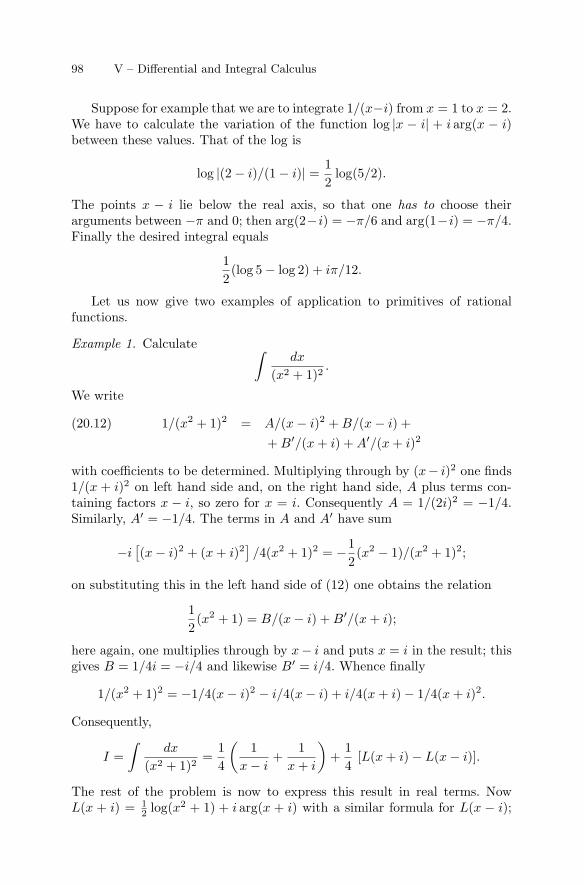
98 V – Differential and Integral Calculus
Suppose for example that we are to integrate 1/(x−i) from x = 1 to x = 2.We have to calculate the variation of the function log |x − i| + i arg(x − i)between these values. That of the log is
log |(2 − i)/(1 − i)| =12
log(5/2).
The points x − i lie below the real axis, so that one has to choose theirarguments between −π and 0; then arg(2−i) = −π/6 and arg(1−i) = −π/4.Finally the desired integral equals
12(log 5 − log 2) + iπ/12.
Let us now give two examples of application to primitives of rationalfunctions.
Example 1. Calculate ∫dx
(x2 + 1)2.
We write
1/(x2 + 1)2 = A/(x − i)2 + B/(x − i) +(20.12)+ B′/(x + i) + A′/(x + i)2
with coefficients to be determined. Multiplying through by (x− i)2 one finds1/(x + i)2 on left hand side and, on the right hand side, A plus terms con-taining factors x − i, so zero for x = i. Consequently A = 1/(2i)2 = −1/4.Similarly, A′ = −1/4. The terms in A and A′ have sum
−i[(x − i)2 + (x + i)2
]/4(x2 + 1)2 = −1
2(x2 − 1)/(x2 + 1)2;
on substituting this in the left hand side of (12) one obtains the relation
12(x2 + 1) = B/(x − i) + B′/(x + i);
here again, one multiplies through by x− i and puts x = i in the result; thisgives B = 1/4i = −i/4 and likewise B′ = i/4. Whence finally
1/(x2 + 1)2 = −1/4(x − i)2 − i/4(x − i) + i/4(x + i) − 1/4(x + i)2.
Consequently,
I =∫
dx
(x2 + 1)2=
14
(1
x − i+
1x + i
)+
14
[L(x + i) − L(x − i)].
The rest of the problem is now to express this result in real terms. NowL(x + i) = 1
2 log(x2 + 1) + i arg(x + i) with a similar formula for L(x − i);
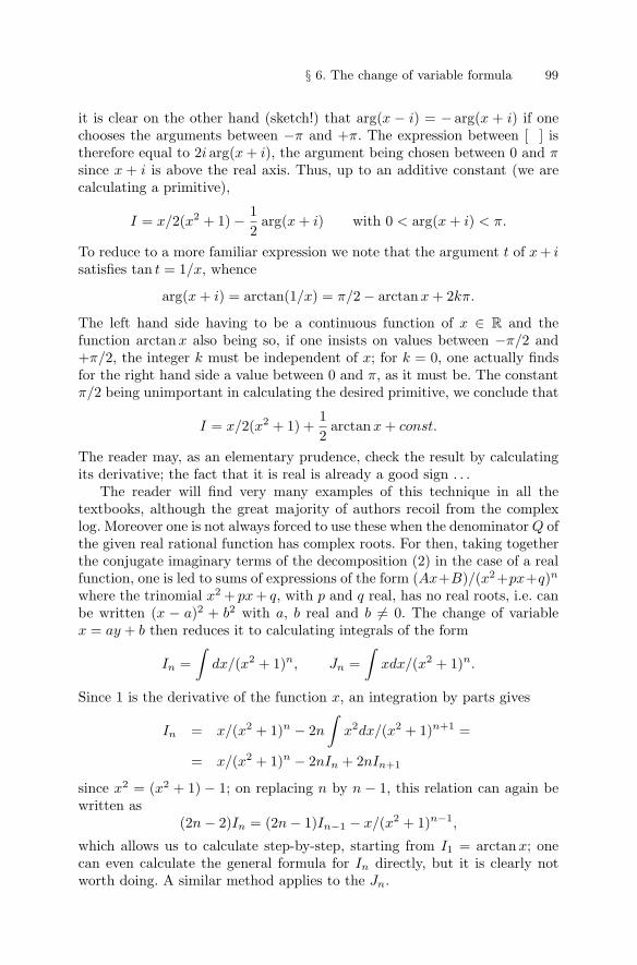
§ 6. The change of variable formula 99
it is clear on the other hand (sketch!) that arg(x − i) = − arg(x + i) if onechooses the arguments between −π and +π. The expression between [ ] istherefore equal to 2i arg(x + i), the argument being chosen between 0 and πsince x + i is above the real axis. Thus, up to an additive constant (we arecalculating a primitive),
I = x/2(x2 + 1) − 12
arg(x + i) with 0 < arg(x + i) < π.
To reduce to a more familiar expression we note that the argument t of x+ isatisfies tan t = 1/x, whence
arg(x + i) = arctan(1/x) = π/2 − arctan x + 2kπ.
The left hand side having to be a continuous function of x ∈ R and thefunction arctanx also being so, if one insists on values between −π/2 and+π/2, the integer k must be independent of x; for k = 0, one actually findsfor the right hand side a value between 0 and π, as it must be. The constantπ/2 being unimportant in calculating the desired primitive, we conclude that
I = x/2(x2 + 1) +12
arctanx + const.
The reader may, as an elementary prudence, check the result by calculatingits derivative; the fact that it is real is already a good sign . . .
The reader will find very many examples of this technique in all thetextbooks, although the great majority of authors recoil from the complexlog. Moreover one is not always forced to use these when the denominator Q ofthe given real rational function has complex roots. For then, taking togetherthe conjugate imaginary terms of the decomposition (2) in the case of a realfunction, one is led to sums of expressions of the form (Ax+B)/(x2+px+q)n
where the trinomial x2 + px + q, with p and q real, has no real roots, i.e. canbe written (x − a)2 + b2 with a, b real and b �= 0. The change of variablex = ay + b then reduces it to calculating integrals of the form
In =∫
dx/(x2 + 1)n, Jn =∫
xdx/(x2 + 1)n.
Since 1 is the derivative of the function x, an integration by parts gives
In = x/(x2 + 1)n − 2n
∫x2dx/(x2 + 1)n+1 =
= x/(x2 + 1)n − 2nIn + 2nIn+1
since x2 = (x2 + 1) − 1; on replacing n by n − 1, this relation can again bewritten as
(2n − 2)In = (2n − 1)In−1 − x/(x2 + 1)n−1,
which allows us to calculate step-by-step, starting from I1 = arctanx; onecan even calculate the general formula for In directly, but it is clearly notworth doing. A similar method applies to the Jn.
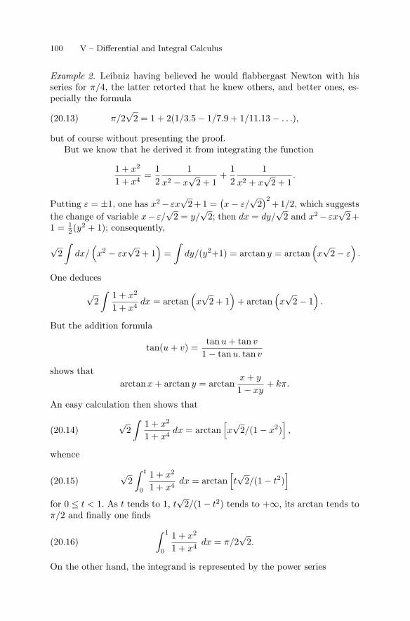
100 V – Differential and Integral Calculus
Example 2. Leibniz having believed he would flabbergast Newton with hisseries for π/4, the latter retorted that he knew others, and better ones, es-pecially the formula
π/2√
2 = 1 + 2(1/3.5 − 1/7.9 + 1/11.13 − . . .),(20.13)
but of course without presenting the proof.But we know that he derived it from integrating the function
1 + x2
1 + x4=
12
1x2 − x
√2 + 1
+12
1x2 + x
√2 + 1
.
Putting ε = ±1, one has x2 − εx√
2+1 =(x − ε/
√2)2
+1/2, which suggeststhe change of variable x− ε/
√2 = y/
√2; then dx = dy/
√2 and x2 − εx
√2+
1 = 12 (y2 + 1); consequently,
√2∫
dx/(x2 − εx
√2 + 1)
=∫
dy/(y2+1) = arctan y = arctan(x√
2 − ε)
.
One deduces
√2∫
1 + x2
1 + x4dx = arctan
(x√
2 + 1)
+ arctan(x√
2 − 1)
.
But the addition formula
tan(u + v) =tan u + tan v
1 − tan u. tan v
shows thatarctan x + arctan y = arctan
x + y
1 − xy+ kπ.
An easy calculation then shows that
√2∫
1 + x2
1 + x4dx = arctan
[x√
2/(1 − x2)],(20.14)
whence
√2∫ t
0
1 + x2
1 + x4dx = arctan
[t√
2/(1 − t2)]
(20.15)
for 0 ≤ t < 1. As t tends to 1, t√
2/(1− t2) tends to +∞, its arctan tends toπ/2 and finally one finds ∫ 1
0
1 + x2
1 + x4dx = π/2
√2.(20.16)
On the other hand, the integrand is represented by the power series
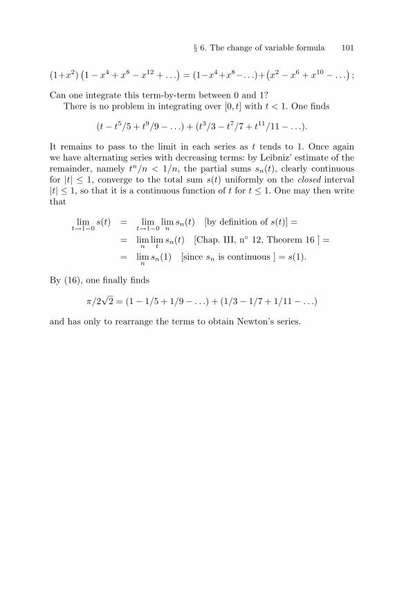
§ 6. The change of variable formula 101
(1+x2)(1 − x4 + x8 − x12 + . . .
)= (1−x4+x8−. . .)+
(x2 − x6 + x10 − . . .
);
Can one integrate this term-by-term between 0 and 1?There is no problem in integrating over [0, t] with t < 1. One finds
(t − t5/5 + t9/9 − . . .) + (t3/3 − t7/7 + t11/11 − . . .).
It remains to pass to the limit in each series as t tends to 1. Once againwe have alternating series with decreasing terms: by Leibniz’ estimate of theremainder, namely tn/n < 1/n, the partial sums sn(t), clearly continuousfor |t| ≤ 1, converge to the total sum s(t) uniformly on the closed interval|t| ≤ 1, so that it is a continuous function of t for t ≤ 1. One may then writethat
limt→1−0
s(t) = limt→1−0
limn
sn(t) [by definition of s(t)] =
= limn
limt
sn(t) [Chap. III, n◦ 12, Theorem 16 ] =
= limn
sn(1) [since sn is continuous ] = s(1).
By (16), one finally finds
π/2√
2 = (1 − 1/5 + 1/9 − . . .) + (1/3 − 1/7 + 1/11 − . . .)
and has only to rearrange the terms to obtain Newton’s series.
102 V – Differential and Integral Calculus
§ 7. Generalised Riemann integrals
Up to now we have attempted to integrate only bounded functions on abounded and, most often, compact interval. To get further we have to freeourselves from these restrictions. The method is quite similar to that for pass-ing from the partial sums to the total sum of a series. To avoid complicationswhich would not be helpful at this level, we restrict ourselves to regulatedfunctions, i.e. those having right and left limits at each point, and so areintegrable on every compact interval (or even bounded interval, if they arethemselves bounded: n◦ 7, corollary to Theorem 6); if we really wanted togeneralise, we would have to go to the grand integration theory (Appendix).This would moreover allow us to simplify many proofs very appreciably, alsothe somewhat artificial statements needed in order to remain at the “elemen-tary” level.
21 – Convergent integrals: examples and definitions
Suppose for example that we wish to assign a meaning to the integral∫ b
0
dx/x.
It is natural, if only for a geometric reason, to consider it as the limit of theintegral over (u, b) as u > 0 tends to 0. This is equal to log b− log u and, hardluck, therefore tends to +∞, which is not the result hoped for, even if, afterall, we have attributed the sum +∞ to divergent series with positive terms.One could also attribute to 1/x the value +∞ at x = 0, so obtaining a lowersemicontinuous function on [0, b] to which one applies the definition of theintegral given in n◦ 11; the result is the same, as one sees on calculating theintegrals over [0, b] of the functions inf(n, 1/x) and then passing to the limitas n → +∞. Replacing 1/x by xs with s real, a function of which a primitiveis xs+1/(s + 1), one obtains the same result if s + 1 < 0. For s + 1 > 0 theintegral over the interval [u, b], equal to bs+1/(s + 1)−us+1/(s + 1), tends tobs+1/(s + 1); whence “clearly”, i.e. by definition,
∫ b
0
xsdx = bs+1/(s + 1) if s > −1 and b > 0.(21.1)
Consider next the integral ∫ +∞
a
xsdx
with a > 0 to eliminate a possible difficulty at x = 0, and where s is real.It is natural to consider this as the limit of the integral over (a, v) as vincreases indefinitely. If s = −1, one finds log v − log a, which tends to +∞.
§ 7. Generalised Riemann integrals 103
If s �= −1, one finds vs+1/(s+1)−as+1/(s+1). If s > −1, the result increasesindefinitely. If s < −1, it tends to −as+1/(s + 1), whence the formula∫ +∞
a
xsdx = −as+1/(s + 1) for s < −1, a > 0.(21.2)
We remark in passing that the hypotheses on s that give a meaning to theintegrals (1) and (2) are mutually exclusive; in other words, the integral∫ +∞
0
xsdx IS NEVER FINITE.
Let us generalise. Let f be a regulated function on a noncompact intervalX = (a, b), either not bounded, or bounded but not closed. If one argues aswe did in defining convergence of a series, one is led to associate a “partialintegral”
s(K) =∫
K
f(x)dx =∫ v
u
f(x)dx = s(u, v) = F (v) − F (u),(21.3)
to every compact interval K = [u, v] contained in X, where F is a primitiveof f in X. We then say that the integral
s(X) =∫
X
f(x)dx =∫ b
a
f(x)dx(21.4)
converges if s(K) tends to a limit – which, by definition, will be the inte-gral (4) – as K “tends to” X, i.e. when u and v tend respectively to40 a andb. As in the case of a series [Chap. II, eqn. (15.4)], this means41 that for everyr > 0 there exists a compact interval K ⊂ X such that, for every compactinterval K ′ ⊂ X,
K ⊂ K ′ =⇒ |s(K ′) − s(X)| < r.(21.5)
One could also then say that f is “integrable” on X, but it is better toabstain carefully from this when the integral of |f | does not converge, thisterm having been reserved, in the only theory which has counted for a longtime, that of Lebesgue, for absolutely integrable functions. It would be betterto speak of semiconvergent integrals when
∫ |f(x)| dx does not converge.(5), again, means that, for every r > 0, one has |s(X)− s(u, v)| < r once
u is close enough to a and v close enough to b. If, for example, a is finite40 If X and f are bounded, in which case f is integrable on X in the sense of n◦ 2
(n◦ 7, corollary to Theorem 6), this definition is compatible with that of n◦ 2.41 One can define this type of limit precisely. Let ϕ(K) be a function of a variable
compact set K ⊂ X. One says that it tends to a limit u as K tends to X iffor every r > 0 there exists a compact K ⊂ X such that K ⊂ K′ ⊂ X =⇒|u − ϕ(K′)| < r. This is definition (21.5).
104 V – Differential and Integral Calculus
and b = +∞, this means that, for every r > 0, there exists an r′ > 0 and anN > 0 such that
{(u − a < r′) & (v > N)} =⇒ |s(X) − s(u, v)| < r.
In terms of primitives,∫ b
a
f(x)dx = limv→b,v<b
F (v) − limu→a,u>a
F (u),(21.6)
so that the integral converges if and only if F has finite limit values at a andb. These limits actually exist if the integral converges, for, in this case, onehas |s(u′, v′) − s(u′′, v′′)| < r if u′ and u′′ are close enough to a and v′ andv′′ close enough to b; taking v′ = v′′, one sees then that |F (u′)−F (u′′)| < r,so that Cauchy’s criterion is satisfied by F (u) as u tends to a. It is clearconversely that the integral converges if F has limits at the end-points of X.
This is exactly what we have verified in the preceding examples. Themethod also works for integrating an exponential function ecx with c realand nonzero, since the behaviour of the primitive ecx/c as x tends to +∞or −∞ has been elucidated in Chap. IV. In particular, one may integrate ex
from −∞ to any finite limit, but one cannot integrate from −∞, nor from afinite limit, to +∞.
But in general one does not know F , so the usefulness of (6) is heavilyconstrained; it is better, in most cases, to examine the order of magnitude off(x) as x tends to a or to b, just as one does for series.
22 – Absolutely convergent integrals
The theory of series is particularly simple when they are absolutely con-vergent. Likewise here. We shall say that the integral (21.4) is absolutelyconvergent if the integral of |f(x)| is convergent, in which case one may saythat f is integrable over X (or, to reassure the reader who is starting thesetopics, absolutely integrable) without risking a collision with the Lebesguetheory.
Theorem 18. (i) Let f be a positive regulated function defined on an inter-val X = (a, b). Then f is integrable on X if and only if the integrals over thecompact subsets K ⊂ X are bounded above; and then∫
X
f(x)dx = supK⊂X
∫K
f(x)dx;(22.1)
(ii) let f be a regulated function defined on an interval X; if the integral∫f(x)dx extended over X is absolutely convergent (i.e. if f is absolutely
integrable on X) then it is convergent and∣∣∣∣∫
X
f(x)dx
∣∣∣∣ ≤∫
X
|f(x)|dx.(22.2)
§ 7. Generalised Riemann integrals 105
To prove point (i) we observe that, f being positive, s(K) is an increasingfunction of K:
K ⊂ K ′ =⇒ s(K) ≤ s(K ′).
The arguments of Chap. II, n◦ 9 on increasing sequences transpose immedi-ately to here without our needing to expound them all again. One might alsoobserve that, if f is positive, its primitives are increasing functions; thesetend to finite limits at the end-points of X if and only if they are boundedon X.
To establish the assertion (ii) one can reduce to the case of a real function,then to that of a positive function by writing f = f+ − f−. Since f+ andf− are majorised by |f |, point (i) shows that the integrals of these functionsconverge, so that of f too. One could also use directly one of the numerousvariants of Cauchy’s criterion adapted to the situation, namely that the par-tial integrals s(K) tend to a limit if and only if for every r > 0 there existsa compact subset K ⊂ X such that
|s(K ′) − s(K ′′)| < r for any K ′ ⊃ K and K ′′ ⊃ K;
but, since K ′ and K ′′ contain K, we have42
|s(K ′) − s(K ′′)| =∣∣∣∣∫
K′−K
f(x)dx −∫
K′′−K
f(x)dx
∣∣∣∣≤∫
(K′−K)∪(K′′−K)
|f(x)|dx,
the integral of |f | being extended over the set (K ′ ∪ K ′′) − K; if we writeS(K) for partial integrals relative to |f | we have
|s(K ′) − s(K ′′)| ≤ S(K ′ ∪ K ′′) − S(K),
an arbitrarily small quantity for any K ′,K ′′ ⊃ K for K “large enough” ifthe S(K) are bounded above.
The inequality (2) is obvious when integrating over a compact intervalK ⊂ X, hence propagates to the limit, qed.
Theorem 18 has some trivial consequences, which we use constantly.
Corollary 1. Let f be a bounded regulated function on an interval X, and µan absolutely integrable regulated function on X. Then the function f(x)µ(x)is absolutely integrable on X and∫
|f(x)µ(x)dx| ≤ ‖f‖X
∫|µ(x)|dx.
42 In what follows, we will have occasion to integrate over a set which is a finiteunion of intervals having, pairwise, at most one point in common; the integral willclearly, by definition, be the sum of the integrals extended over these intervals.This, furthermore, is equivalent to multiplying the integrand by the characteristicfunction, a step function, of this union.
106 V – Differential and Integral Calculus
Obvious. As we shall do on various occasions in the rest of this §, we haveused the
∫sign to denote integrals extended over X.
Example: the Fourier transform
µ(y) =∫
R
e−2πixyµ(x)dx(22.3)
of an absolutely integrable function on X = R is defined for every y ∈ R.In the following statement one says that a function f is square (under-
stood: absolutely) integrable on an interval X if the function |f |2 is integrableon X. One may then generalise Cauchy-Schwarz:
Corollary 2. Let f and g be two regulated square integrable functions on aninterval X; then the function f(x)g(x) is absolutely integrable on X and∣∣∣∣
∫f(x)g(x)dx
∣∣∣∣2 ≤∫
|f(x)|2dx.
∫|g(x)|2dx.
One replaces f and g by |f | and |g|, writes the Cauchy-Schwarz inequalityfor every compact interval K ⊂ X and notes that the left hand side is, forany K, majorised by the right hand side of the inequality to be established,whence the result on passage to the limit. Or else, see the end of n◦ 14, whichwill prove more generally that if the functions |f |p and |g|q are integrable for1/p + 1/q = 1, then fg is also integrable, and a Holder inequality is valid.
The convergence conditions for the integrals involving xs establishedabove for s real can be transformed immediately into conditions for absoluteconvergence in the case of a complex exponent, since
|xs| = xRe(s) for x > 0.
On the other hand, point (ii) of Theorem 18 shows that if, on a neighbourhoodof one of the limits of integration, one has a relation of the form
f(x) = O(g(x)),
then absolute convergence (on a neighbourhood of this end-point) of theintegral of g(x) implies that of the integral of f(x); if one has the moreprecise relation f(x) � g(x) then the integrals are of the same nature asconcerns absolute convergence. (It might, on the other hand, happen thatone of them converges non-absolutely and that the other diverges, as canoccur with series.)
In elementary practice the absolute convergence of an integral is almostalways shown by comparing the behaviour of the integrand with that of acombination of classical functions: exponentials, powers, logarithms, etc. Itis worth having these results permanently available, and to have understoodtheir reasons.
§ 7. Generalised Riemann integrals 107
First of all, putting X = (a, b), one may always choose a c such that a <c < b and decompose the integral into integrals extended over (a, c) and over(c, b). If the integrand is regulated there will be no problem of convergenceon a neighbourhood of c, and this allows us to isolate the difficulties. Onemay always, in the case where c is the right endpoint, reduce to the casewhere c = +∞ by the change of variable c−x = 1/y. If c is the left endpoint,one may reduce to the case where c = 0 by x − c = y, or to c = −∞ byx − c = −1/y.
Now consider the prototype integral∫ +∞
a
logm x.xne−sxdx (a > 0)(22.4)
where m, n, s are a priori complex but can in fact be assumed real, sincethe modulus of the integrand is obtained by replacing the exponents by theirreal parts. In view of the orders of increase of the three functions involved,it is pretty clear that the convergence of the integral is, for s �= 0, governedby the exponential factor. It follows immediately from Chap. IV, n◦ 5, that
logm x.xn = o(erx) as x → +∞ for every r > 0;
the integral will thus converge if there exists an r > 0 making the integralof e(r−s)x converge, i.e. if r − s < 0, whence convergence for s > 0, strictinequality. For s < 0, the integrand grows indefinitely, whence divergence.
In the case where s = 0, the change of variable x = ey leads us to integratethe function yme(n+1)y on a neighbourhood of infinity; the integral is thusconvergent for n < −1 and divergent for n > −1.
If, finally, we have n = −1, so that we are dealing with the integral ofx−1 logm x, the same change of variable reduces to the function ym, whenceconvergence for m < −1 and divergence for m ≥ −1.
In conclusion, convergence is governed by the exponential function if thisis actually present or, if it is absent (s = 0), by the power function if that isactually present; if these two functions are absent, the integral converges ifand only if m < −1.
One might study integrals similar to (4), but containing more simplefactors, by the same method; you could, for example, introduce the factorslog log x, or log log log x, etc. . . ., which grow more and more slowly and donot affect the result so long as there are factors present which decrease muchmore rapidly than them. You might also insert a factor x−x, which tendsto 0 fast enough to annihilate even the most vertical exponential functions. . . Etc.
The study of an integral such as∫ b
0
| log x|mxndx (0 < b < +∞)(22.5)
108 V – Differential and Integral Calculus
reduces to the preceding case; the change of variable x = 1/y transforms itinto the integral of the function logm y.y−n−2 on a neighbourhood of +∞.The integral (5) is thus convergent if −n− 2 < −1, i.e. if n > −1; it divergesif n < −1. If n = −1, the integral converges if m < −1 and diverges inthe contrary case. Note in passing that (5) always converges for n = 0, i.e.when the term xn is absent, a result due to the fact that on a neighbourhoodof 0 a power of the log grows less quickly than any negative power of x, forexample than the function x−1/2 whose integral converges (primitive: 2x1/2).For n = 0, m = 1, note that log x has primitive x log x− x, a function whichtends to a limit, namely 0, when x → 0.
Exercise: extend this calculation to the case of an arbitrary integer m > 0by integrating by parts.
The case of rational functions is particularly simple: if p and q are poly-nomials and q has no real roots then the absolute convergence of the integral∫ +∞
−∞
p(x)q(x)
dx
depends only on the integer n = d◦(q)−d◦(p) since the function is equivalentto 1/xn to within a constant factor; so absolute convergence is equivalent tothe condition n ≥ 2.
Example 1. Consider Euler’s ubiquitous Gamma function
Γ (s) =∫ +∞
0
e−xxs−1dx.(22.6)
Absolute convergence at infinity is automatic, but, at 0, requires Re(s) > 0.An integration by parts43 then shows that
Γ (s + 1) =∫ +∞
0
e−xxsdx = −e−xxs
∣∣∣∣+∞
0
+ s
∫ +∞
0
e−xxs−1dx
and since the integrated-out part is clearly zero, we have
Γ (s + 1) = sΓ (s).(22.7)
Since it is clear that Γ (1) = 1 we deduce that
Γ (n) = (n − 1)!(22.8)
for every integer n > 1. This is Euler’s method for defining the “factorial” ofan arbitrary complex number. We shall see in n◦ 25 that the Γ function isholomorphic in the half plane Re(s) > 0 and that it is even the restriction ofa function holomorphic on C − {0,−1,−2, . . .} .43 The formula
∫f ′g = fg − ∫ fg′ for integration by parts applies to the integrals
considered here, on condition that we check that the function fg has limit valuesat the end-points of the interval of integration X: integrate over a compactK ⊂ X and pass to the limit.
§ 7. Generalised Riemann integrals 109
Example 2. Euler also studied the integral
B(x, y) =∫ 1
0
tx−1(1 − t)y−1dt(22.9)
where x and y are a priori complex (and rational for him). Absolute conver-gence on a neighbourhood of 0 requires Re(x) > 0 and, on a neighbourhoodof 1, Re(y) > 0. Clearly
B(x, y) = B(y, x)(22.10)
(change of variable t → 1 − t). The change of variable t → sin2 t shows that
B(x, y) = 2∫ π/2
0
sin2x−1 t. cos2y−1 t.dt.(22.11)
We shall see later (n◦ 26, Example 1) that
B(x, y) = Γ (x)Γ (y)/Γ (x + y),(22.12)
a famous formula due to Euler with, as always, a proof which posterity,principally Jacobi, has rectified. It immediately provides the explicit value of(11) for x, y ∈ N.
23 – Passage to the limit under the∫
sign
For generalised or “improper” Riemann integrals there are theorems on pas-sage to the limit which the Lebesgue theory has rendered obsolete, but remainusable at a more elementary level. For example:
Theorem 19 (Poor man’s dominated convergence). Let (fn) be a se-quence of regulated functions, absolutely integrable on an interval X ⊂ R.Assume that
(i) the fn converge to a limit f uniformly on every compact K ⊂ X,(ii) there exists a positive function p, integrable on X, and such that
|fn(x)| ≤ p(x) for any x and n.Then the function f is absolutely integrable on X and∫
f(x)dx = lim∫
fn(x)dx.(23.1)
First of all, it is clear that f , being regulated like the fn, is absolutelyintegrable on X since |f(x)| ≤ p(x) for every x. Since p is positive andintegrable, for every r > 0 there exists a compact interval K ⊂ X such that∫
X−K
p(x)dx < r(23.2)
110 V – Differential and Integral Calculus
(and even for every K ′ ⊃ K), whence the same relation for each |fn(x)| andfor |f(x)|. On the other hand∫
K
|f(x) − fn(x)|dx < r for n large(23.3)
since fn converges uniformly to f on K. Now∣∣∣∣∫
X
f(x)dx −∫
X
fn(x)dx
∣∣∣∣ ≤∫
X
|f(x) − fn(x)|dx
is the sum of the analogous integrals extended over K and X − K; by (2),the second is < 2r since |f(x) − fn(x)| ≤ 2p(x) for any x and n; the first is< r for n large by (3). The left hand side of the preceding relation (and eventhe right hand side) thus tends to 0, qed.
Example 1. Consider the function
Γ (s) =∫ +∞
0
e−xxs−1dx, Re(s) > 0,
again, and observe that
e−xxs−1 = lim(1 − x/n)nxs−1.
We cannot just bluntly apply Theorem 19 since the functions on the righthand side are not integrable between 0 and +∞: convergence at 0 presupposesRe(s) > 0 and convergence at infinity Re(s) < −n. For x < n we always have[Chap. III, n◦ 16]
log[(1 − x/n)n] = n. log(1 − x/n) = −x − x2/2n − . . . < −x
and so (1 − x/n)n < e−x. Now consider the functions
fn(x) ={
(1 − x/n)nxs−1 for 0 < x ≤ n,0 for x > n;(23.4)
they converge to the absolutely integrable function e−xxs−1 and satisfy|fn(x)| ≤ |e−xxs−1|. To be able to apply Theorem 19 it therefore sufficesto show that convergence is uniform on every compact subset of ]0, +∞[. Ifwe accept this point provisionally we then find
Γ (s) = lim∫ n
0
(1 − x/n)nxs−1dx = limns
∫ 1
0
(1 − u)nus−1du;
on integrating by parts a la Leibniz, i.e. without limits of integration, we findthat ∫
(1 − u)nus−1du = (1 − u)nus/s +n
s
∫(1 − u)n−1usdu
§ 7. Generalised Riemann integrals 111
and since the integrated-out part is zero for u = 0 [because Re(s) > 0] andu = 1, we find ∫ 1
0
(1 − u)nus−1du =n
s
∫ 1
0
(1 − u)n−1xsdx;
whence, iterating,∫ 1
0
(1 − u)nus−1du =n!
s(s + 1) . . . (s + n).(23.5)
A little less than two centuries after 1812 and Gauss, who did not knowthat Euler, ever present, had preceded him along this path about 1776, asRemmert, Funktionentheorie 2, pp. 34–36, tells us, we find that
Γ (s) = limn!ns/s(s + 1) . . . (s + n)(23.6)
for Re(s) > 0. We can derive an expansion of Γ as an infinite product, butwe still lack the necessary “Euler’s constant” which will appear in Chap. VI,n◦ 18.
We still have to show that the functions (4) converge uniformly on everycompact interval K = [a, b] with 0 < a < b < +∞. The factor xs−1 beingbounded on K since a > 0, it is enough to examine the factor (1 − x/n)n.For n > b we have |x/n| < 1 in K and thus
log [(1 − x/n)n] = n. log(1 − x/n) = − (x + x2/2n + x3/3n2 + . . .);
the sequence of functions log [(1 − x/n)n], thus also that of the functions(1 − x/n)n, is therefore increasing on K, and even on [0, b], for n > b. Sinceit converges to the continuous function e−x uniform convergence on K followsfrom Dini’s Theorem of n◦ 10.
More elementarily, so more complicated: first remark that log [(1 − x/n)n] =−x − x2/2n − . . . converges uniformly to −x on [0, b], since, for n > b,
∣∣x2/2n + x3/3n2 + . . .∣∣ ≤ b2
n
(1 + b/n + b2/n2 + . . .
)=
b
n − b
for every x ∈ [0, b]. Since (1− x/n)n = exp[n. log(1− x/n)], it remains eitherto “dirty one’s hands” by calculating (exercise!), or to establish a generallemma to bypass the calculations:
Lemma. Let K be a compact subset of C, let (fn) be a sequence of functionswhich converges uniformly on K to a bounded limit function f on K, andlet g be a function defined and continuous on an open set U containing theclosure of f(K). Then the composite function gn = g ◦fn is defined on K forn large and converges uniformly to g ◦ f .
112 V – Differential and Integral Calculus
The limit f being bounded, the closure H of f(K) is compact so that,for every integer p, the set Hp of the z ∈ C such that d(z,H) ≤ 1/p isalso compact. Since U is open and contains H, it contains44 an Hp. Since‖f−fn‖K ≤ 1/p for n large, we therefore have fn(K) ⊂ Hp ⊂ U , which allowsus to define gn(x) = g[fn(x)]. Now the function g is uniformly continuouson the compact Hp; for every r > 0 there is therefore an r′ > 0 such that|g(z′) − g(z′′)| ≤ r if z′, z′′ ∈ Hp satisfy |z′ − z′′| ≤ r′; now this, for n large,is the case for any x ∈ K if one takes z′ = f(x) and z′′ = fn(x). Hence‖g ◦ f − g ◦ fn‖K ≤ r for n large, qed.
Note in passing that the lemma makes no hypothesis as to the nature ofthe fn; in particular, they are not assumed continuous; it is g which must be.But if the fn are continuous, the function f is so too, and the closure H off(K) is in fact the compact set f(K) itself.
If, instead of integrating a sequence of functions one integrates a series,one has to consider the partial sums sn(x) of the series and apply the pre-ceding theorem to them. The simplest result is the following:
Theorem 20. Let∑
un(x) be a series of absolutely integrable regulatedfunctions on an interval X. Assume that (i) the series converges uniformlyon every compact K ⊂ X; (ii) there exists a positive function p(x), inte-grable on X, such that
∑ |un(x)| ≤ p(x) for every x ∈ X. Then the functions(x) =
∑un(x) is absolutely integrable on X and∫
s(x)dx =∑∫
un(x)dx.(23.7)
The hypothesis (i) shows that the partial sums sn(x) converge uniformlyon every compact K ⊂ X; since (ii) shows that |sn(x)| ≤ p(x), one need onlyapply the preceding theorem to the sn.
Condition (ii) is analogous to normal convergence on all of X, but morerestrictive. In fact, and in contrast to the case of integrals extended over acompact interval, normal convergence in X is not enough to assure (7) ifX is not bounded. We do know then, of course, that for n large the differ-ence between the total sum s(x) and the partial sum sn(x) is < r for anyx ∈ X since this is majorised by the n-th remainder of the series
∑vn which
dominates the series∑
un(x). But we cannot extract any estimate for thedifference between their integrals over X if X is not bounded.
One may however establish a useful result whose formulation is very closeto that of one of the fundamental results of the Lebesgue theory:44 The Hp ∩ (C − U) are closed and bounded and form a decreasing sequence of
compacta; their intersection, contained simultaneously in H (because H = ∩Hp
for every compact H) and in C−U , is empty; thus Hp∩(C−U) = ∅, i.e. Hp ⊂ U ,for p large: Chap. III, n◦ 9 or corollary 1 of BL.
§ 7. Generalised Riemann integrals 113
Theorem 21. Let X be an interval and un(x) a series of regulated functionswhich converges normally on every compact K ⊂ X. Assume that
∑∫|un(x)|dx < +∞.(23.8)
Then the function s(x) =∑
un(x) is absolutely integrable on X and∫s(x)dx =
∑∫un(x)dx.
Let us put, generally,
mI(f) =∫
I
f(x)dx
and consider a compact interval K ⊂ X. Since the given series convergesnormally on K (“uniformly” would suffice) and one may integrate term-by-term on a compact set (n◦ 4), the relation |s(x)| ≤∑ |un(x)| shows that
mK(|s|) ≤ mK
(∑|un|)
=∑
mK(|un|) ≤∑
mX(|un|) = M < +∞
by (8). The regulated function s is therefore absolutely integrable on X [The-orem 18, (i)], with mX(|s|) ≤∑mX(|un|). Omitting the first N terms fromthe series, one finds in the same way that
mX
(∣∣∣s − N∑p=1
up
∣∣∣) ≤ ∞∑p=N+1
mX(|un|).
The result is ≤ r for N large since∑
mX(|un|) < +∞. It follows that
∣∣∣mX(s) −N∑
p=1
mX(up)∣∣∣ ≤ mX
(∣∣∣s − N∑p=1
up
∣∣∣) ≤ r for N large,
whence the theorem.In the Lebesgue theory, the two preceding theorems are valid without the
hypothesis of uniform or normal convergence, which would considerably sim-plify the arguments of Example 1; simple (or even only “almost everywhere”)convergence is enough to assure the result; in fact, the hypothesis (8) evenimplies “almost everywhere” absolute convergence of the series
∑un(x), as
we shall see. On the other hand, hypothesis (ii), “dominated convergence”,is essential even in the “grand” integration theory, where one ignores (in theEnglish sense) the “semiconvergent” integrals, so specific to R.
Instead of integrating a function of x depending on an integer n one mayconsider more generally an integral of the form
114 V – Differential and Integral Calculus
∫X
f(x, y)dx
where y varies in an arbitrary subset Y of R or even of C, and examine whathappens when y tends to a closure point b of Y . The hypotheses to make areobvious:
(i) the function x → f(x, y) is regulated for every y;(ii) limy→b f(x, y) = g(x) exists for every x ∈ X and the limit is uniform on
every compact K of X, i.e. for every r > 0 there is an r′ > 0 such that
|f(x, y) − g(x)| ≤ r for every x ∈ K
for every y such that |y − b| ≤ r′;(iii) there exists a positive integrable function p on X such that |f(x, y)| ≤
p(x) on X for every y ∈ Y close enough to b.
Then we may write
limy→b
∫f(x, y)dx =
∫dx lim
y→bf(x, y).
The hypotheses (i), (ii) and (iii) show that g is regulated and absolutelyintegrable, after which it is enough to copy the proof of Theorem 21, replacingfn(x) everywhere by f(x, y) and the expression “for n large” by “for y closeenough to b” (or “for y large” if y tends to infinity). We could have establishedthis general result directly; the theorem for sequences can be deduced fromit on taking Y = N and b = +∞.
In the most frequent applications of this result one seeks to show that theintegral is a continuous function of y:
Theorem 22. Let X be an interval, H a compact subset of C, f a functiondefined and continuous on X × H and µ a function defined and regulated inX. Assume that there is a positive function p on X such that |f(x, y)| ≤ p(x)on X×H and
∫p(x)|µ(x)|dx < +∞. Then the function y → ∫ f(x, y)µ(x)dx
is continuous on H.
Hypotheses (i) and (iii) above are clearly satisfied by f(x, y)µ(x) wheny tends to a b ∈ H. If K is a compact subset of X, then the function f isuniformly continuous on the compact K × H; consequently, the hypothesis(ii) is satisfied also45. Thus lim
∫f(x, y)µ(x)dx =
∫f(x, b)µ(x)dx, qed.
45 Recall why. For every r > 0 there exists an r′ > 0 such that the values of f attwo points of K × H distant at most r′ from each other are equal to within r.It follows that |y − b| < r′ =⇒ |f(x, y) − f(x, b)| < r for every x ∈ K, whichmeans that, as y tends to b, f(x, y) tends to f(x, b) uniformly on K. The factorµ(x), which is bounded on every compact set, like every regulated function, doesnot change the conclusion. Note in passing that if we have introduced a functionµ(x), it is because we do not yet know how to treat an integral
∫f(x, y)dµ(x)
with respect to an arbitrary measure on a noncompact interval.
§ 7. Generalised Riemann integrals 115
In practice, the continuous function f is defined on X × Y where Y ⊂ Cis not necessarily compact: the case of an arbitrary interval in R or of anopen subset of C for example. To apply the theorem, it is enough to workon an arbitrarily small neighbourhood of a point b ∈ Y since continuity is aproperty of local nature. So everything works if every b ∈ Y has a compactneighbourhood in Y . Now a neighbourhood of b in Y contains, by definition,all the points of Y whose distance to b is sufficiently small. The hypothesisin question thus means that there exists an r > 0 such that the set of y ∈ Ysuch that d(b, y) ≤ r (weak inequality) is compact. A subset of C having thisproperty at each of its points is said to be locally compact. This is the caseif Y = F ∩ U with F closed and U open46: choose r so that the closed discd(b, y) ≤ r is in U , then take for a neighbourhood of b in Y the intersection ofthis disc with F : it is closed in C, so compact. In R, every interval is locallycompact; Q is not (exercise!). In C, the union Y of the open disc D : |z| < 1and of the compact interval [1, 3] is not, even though both these two sets are:the intersection of Y with a closed disc of centre 1 is never closed. We mighthave said all this in Chap. III, but the reader is perhaps grateful to have beenspared this at the beginning of the theory . . .
In conclusion, Theorem 22 remains valid if one assumes H only locallycompact. By a happy coincidence, the locally compact sets are, among thesubsets of C, those on which one may construct an integration theory a laLebesgue and, for a start, give a reasonable definition of Radon measures, aswe shall see in n◦ 31.
24 – Series and integrals
One may sometimes compare an integral to a series, and vice-versa, to decideon its convergence or divergence. If, for example, f is a regulated function onan interval X = [a,+∞[ with a finite, then f has a limit value at a and theconvergence of the integral on a neighbourhood of a poses no problem; it isthen clear that∫
X
|f(x)|dx < +∞ ⇐⇒∑n≥a
∫ n+1
n
|f(x)|dx < +∞
because the partial sums of the series are, more or less, the partial integralsover the intervals [a, n].
Consider now a function f defined for x ≥ a finite, positive, decreasing,and tending to 0 at infinity (without this, for a decreasing function, theintegral has no chance of converging); being monotone, f is regulated (and,in applications, is always continuous). For every n ≥ a the integral of f overthe interval [n, n + 1] lies between f(n) and f(n + 1) since f is positive anddecreasing. The series (1) is therefore of a similar nature to the series
∑f(n)
46 One can prove the converse, but it is hardly worthwhile.
116 V – Differential and Integral Calculus
and consequently, the integral of f on the interval [a,+∞] converges if andonly if the series
∑f(n) converges, with
∑n≥a
f(n) ≤∫ +∞
a
f(x)dx ≤ f(a) +∑n>a
f(n);(24.1)
the term f(a) comes from the interval [a, p] where p is the smallest integer≥ a. A sketch will make the result obvious.
If for example f(x) � c/xs with s real, the integral converges like theRiemann series
∑1/ns, i.e. for s > 1.
There are also the integrals of “oscillating” functions. Consider for exam-ple the integral
I =∫ +∞
a
f(x) sin(πx)dx(24.2)
where f is again positive, decreasing, and tends to 0 at infinity. The integralbetween n and n+1 this time lies up to sign between f(n) and f(n + 1) since,on the interval considered, sin(πx) is either everywhere between 0 and 1, oreverywhere between −1 and 0. This suggests comparison with the alternatingseries∑
(−1)nf(n), which converges since f decreases and tends to 0. But itis better to compare with the series with general term
un =∫ n+1
n
f(x) sin(πx)dx.
It is clear that the un are alternately positive and negative. On the otherhand
un+1 = −∫ n+1
n
f(x + 1) sin(πx)dx
thanks to the change of variable x → x+1. Since f(x+1) ≤ f(x), we concludethat |un+1| ≤ |un|. Finally, and as we have seen, |un| always lies between f(n)and f(n+1), so tends to 0. The alternating series un is therefore convergent.Now let p be the smallest integer ≥ a. For p ≤ n ≤ v < n + 1 we have∫ v
a
f(x) sin(πx)dx =∫ p
a
. . . + (up + . . . + un−1) +∫ v
n
f(x) sin(πx)dx.
Since the last integral is, in modulus, ≤ f(n) and so tends to 0, and sincethe series un converges, it is clear that the left hand side tends to a limit asv → +∞, namely
I =∫ p
a
f(x) sin(πx)dx +∑n≥p
un.
The “remainder” of an alternating series being, in absolute value, less thanthe first term neglected, one thus obtains, for every n > a, the inequality
§ 7. Generalised Riemann integrals 117
∣∣∣∣I −∫ n
a
f(x) sin(πx)dx
∣∣∣∣ ≤ f(n).(24.3)
From this one can deduce an important result on the Fourier transform:
Theorem 23. Let f be a positive regulated function, defined for x ≥ a > −∞,decreasing, and tending to 0 at infinity. Then the integral
ϕ(y) =∫ +∞
a
f(x) sin(2πxy)dx
converges for any y �= 0, and is a continuous function of y.
To see this, assume y > 0 and perform the change of variable 2xy = u,whence
2yϕ(y) =∫ +∞
2ay
f(u/2y) sin(πu)du.
Convergence is clear, and (3) can now be written∣∣∣∣2yϕ(y) −∫ n
2ay
f(u/2y) sin(πu)du
∣∣∣∣ ≤ f(n/2y).(24.4)
Let us work on an interval y ≥ b > 0. We have f(n/2y) ≤ f(n/2b), so thatf(n/2y) converges uniformly to 0 on this interval. Thus it remains to showthat the integral in (4) is a continuous function of y for any n; for then 2yϕ(y)will be the uniform limit of continuous functions on y > b. Now, returning tothe initial variable of integration x = u/2y, the integral in question can bewritten ∫ n/2y
a
sin(2πxy)f(x)dx,
and its continuity as a function of y is clear, even though the upper limit ofintegration depends on y. The reader may provide the ε, inspired by Theo-rem 13 of n◦ 12.
Dirichlet’s integral ∫ +∞
0
sin(2πxy)dx/x
fits into this framework, for the function sin(2πxy)/x tends to 2πy at theorigin, so that it is enough to examine its behaviour at infinity, given by thepreceding theorem. (Note that in fact the integral does not depend on y).Same remark for the Fresnel integrals of the kind∫ +∞
0
cos(2πx2y)dx, y �= 0;
the change of variable x2 = t leads to
118 V – Differential and Integral Calculus
∫ +∞
0
cos(2πyt)t−1/2dt;
there is no problem at t = 0 since − 12 > −1. The problem is to calculate the
integral explicitly.The preceding theorem applies also to the Fourier integrals
f(y) =∫ +∞
−∞f(x)e−2πixydx,
which, by Euler’s formulae, reduce to four integrals of the preceding type.Theorem 25 thus applies here when f(x) tends to 0 at infinity in a monotonefashion for |x| large: the integral converges for y �= 0 and f(y) is continuous onR∗ = R−{0}. This is the case, for example, if f(x) = p(x)/q(x) is a rationalfunction for which d◦(q) = d◦(p) + 1; the function f tends to 0 monotonelyat infinity because its derivative has only a finite number of roots, so hasconstant sign on a neighbourhood of +∞ or −∞. We should not forget thatthe integral does not converge absolutely.
25 – Differentiation under the∫
sign
To extend the theorem on differentiation under the∫
sign to “improper”integrals one considers as in n◦ 9 a continuous function f on a rectangleX × J where, this time, X is no longer compact, and one assumes that D2fexists and is continuous on X × J . In ignorance of what a measure is onemay always examine an integral of the form
g(y) =∫
f(x, y)µ(x)dx,(25.1)
where µ is a regulated function on X, and seek hypotheses to assure that
g′(y) =∫
D2f(x, y)µ(x)dx.(25.2)
We assume of course that (1) and (2) are convergent integrals for any y ∈ J . Inproblems of this kind the principle is the same as for the analogous problemsfor series: one replaces X = (a, b) by a compact interval K = [u, v] containedin X, applies Theorem 9 of n◦ 9 to the function47
gK(y) =∫
K
f(x, y)µ(x)dx,(25.3)
47 We remarked at the end of n◦ 9 that Theorem 9 does not rest on the explicitconstruction of the usual integral, but only on its properties of linearity andcontinuity. These would be equally valid if one defined the integral by the for-mula µ(f) =
∫f(x)µ(x)dx. Theorem 9 does not apply directly to the function
f(x, y)µ(x), since it is no longer necessarily continuous, but the result still holds.
§ 7. Generalised Riemann integrals 119
then one passes to the limit as u and v tend respectively to a and b, i.e. asK tends to X. Since
g′K(y) =∫
K
D2f(x, y)µ(x)dx(25.4)
by Theorem 9 of n◦ 9, we have to show that the derivative of a limit is thelimit of the derivatives, a problem which Theorem 19 of Chap. III, n◦ 17 isthere to resolve: since gK(y) tends to g(y) for every y, it is enough to showthat g′K(y) converges to the integral (2) uniformly on every compact subsetH of J as K tends to X. Equivalently, that for every r > 0 there exists acompact interval K ⊂ X such that∣∣∣∣
∫X−K′
D2f(x, y)µ(x)dx
∣∣∣∣ ≤ r for every y ∈ H and every K ′ ⊃ K;(25.5)
the integral (5) is actually the difference between g′K(y) and the integral (2)to which it must converge [and which we will have the right to denote g′(y)after having justified the passage to the limit]. A brutal way of guaranteeing(5) is to assume the existence of a positive function pH(x) such that
|D2f(x, y)| ≤ pH(x) with∫
X
pH(x)|µ(x)|dx < +∞(25.6)
for any x ∈ X and y ∈ H; the left hand side of (5) is then majorised by theintegral of pH |µ| over X −K ′, so is < r for any y ∈ H if K ′ contains a largeenough compact interval K ⊂ X.
This is the argument used to show that if, for a series of differentiablefunctions the series of its derivatives converges normally, then one may dif-ferentiate it term-by-term. The integrals of D2f on the compact sets playthe role of the partial sums of the derived series; the existence of a functionpH satisfying (3) plays the role of normal convergence and guarantees thatfor K ⊂ X large enough the “remainder” of the “sum” of the D2f(x, y), i.e.the integral on X −K, is in modulus ≤ r for any y. One cannot recommendthe reader too strongly to let himself be guided by these analogies between“continuous sums”, i.e. integrals, and “discrete sums”, i.e. series.
We thus obtain a simple but useful result:
Theorem 24. Let X and J be two intervals in R, let µ be a regulated func-tion on X and f a function defined and continuous on X × J . Assume that
(i) the integral
g(y) =∫
X
f(x, y)µ(x)dx
converges for every y ∈ J ;(ii) the function f has a continuous partial derivative D2f(x, y) on X × J ;
120 V – Differential and Integral Calculus
(iii) for every compact H ⊂ J there exists a positive function pH on Xsuch that |D2f(x, y)| ≤ pH(x) for every x ∈ X and every y ∈ H, and∫
pH(x)|µ(x)|dx < +∞.
Then the function g is differentiable and
g′(y) =∫
X
D2f(x, y)µ(x)dx.(25.7)
Example 1. If X = Y = R, if µ is an absolutely integrable regulated functionon R and if f(x, y) = e−2πixy, then the function g(y) is just the Fouriertransform µ of µ. Here
D2f(x, y) = −2πixe−2πixy
and so |D2f(x, y)| = 2π|x| = p(x), and this is clearly the smallest positivefunction which dominates x → D2f(x, y) for a (or for all) y ∈ Y . Conclusion:if ∫
R
|xµ(x)|dx < +∞,
then µ is differentiable and
µ′(y) = −2πi
∫R
xµ(x)e−2πixydx
is the Fourier transform of −2πixµ(x).
Example 2. In particular choose µ(x) = exp(−πx2), an integrable functionon R since it decreases at infinity more rapidly than |x|−n for any n > 0. Wehave −2πixµ(x) = iµ′(x), whence, integrating by parts,
µ′(y) = i
∫ +∞
−∞µ′(x) exp(−2πixy)dx = −2πy
∫ +∞
−∞µ(x) exp(−2πixy)dx
since the integrated-out part is zero because of the decrease of µ at infinity.One obtains the relation
µ′(y) = −2πyµ(y),
a relation satisfied equally by µ. The function µ/µ therefore has derivativezero, whence
µ(y) = cµ(y) = c exp(−πy2)(25.8)
with a constant
c = µ(0) =∫
R
exp(−πx2)dx.(25.9)
§ 7. Generalised Riemann integrals 121
It will emerge later that c = 1, and this without the least calculation, thanksto the general Poisson summation formula∑
µ(n) =∑
µ(n),
where the sums are over Z. In part this explains the role of the functionexp(−πx2) in the calculus of probabilities (Gauss’ normal law).
The preceding theorem can be used to show that a function is holomor-phic:
Theorem 24 bis. Let X be an interval in R, U an open subset of C, µ aregulated function in X, and f a function defined and continuous on X × Usatisfying the following conditions:
(i) the integral
g(z) =∫
X
f(t, z)µ(t)dt
converges absolutely for every z ∈ U ;(ii) the function z → f(t, z) is holomorphic on U for every t ∈ X and its
derivative f ′(t, z) with respect to z is continuous on X × U ;(iii) for every compact H ⊂ U , there exists on X a positive function pH(t)
such that |f ′(t, z)| ≤ pH(t) for every t ∈ X and every z ∈ H and∫pH(t)|µ(t)|dt ≤ +∞.
Then g is holomorphic on U and
g′(z) =∫
X
f ′(t, z)µ(t)dt.(25.10)
Putting z = x + iy, Theorem 24 shows that one may differentiate underthe∫
sign, either with respect to x for y given, or with respect to y for x given.Since z → f(t, z) satisfies the Cauchy’s holomorphy condition [Chap. II, eqn.(19.10)], so clearly g does too, qed.
Example 3. If µ is a regulated function on the closed interval [0,+∞[ andis O(tN ) at infinity for some N , its Laplace transform or complex Fouriertransform
Lµ(z) =∫ +∞
0
e2πitzµ(t)dt
is defined on U : Im(z) > 0 since then |e2πitzµ(t)| = O(e−2πtytN ) at infinity.Here f(t, z) = e2πitz, whence |f ′(t, z)| = 2πte−2πty. Since every compactsubset H of U is contained in a half plane Im(z) ≥ σ > 0, we have, in H,that |f ′(t, z)| ≤ 2πte−2πσt = pH(t) with
∫pH(t)|µ(t)|dt < +∞ since the
function pH(t)µ(t) = O(e−2πσttN+1) is absolutely integrable on R+. Thefunction Lµ is therefore holomorphic on U .
122 V – Differential and Integral Calculus
This calculation, iterated, shows further that the (complex) derivativesof Lµ are given by
L(n)µ (z) = (2πi)n
∫ +∞
0
e2πitztnµ(t)dt.(25.11)
Example 4. The function Γ (s) =∫
e−xxs−1dx is holomorphic in the halfplane Re(s) > 0 where it is defined. It is clear that
(i) the function s → e−xxs−1 = e−x exp[(s − 1) log x] is holomorphic forevery x > 0 since it is the composite of two holomorphic functions;
(ii) its complex derivative48 e−xxs−1 log x is continuous;(iii) if s remains in a compact subset H of the half plane Re(s) > 0, strict
inequality, then s is subject to conditions a ≤ Re(s) ≤ b with 0 < a <b < +∞, so that
∣∣e−xxs−1 log x∣∣ ≤ pH(x) =
{e−xxa−1| log x| if 0 < x ≤ 1,e−xxb−1 log x if 1 < x < +∞ .
Now the integral of xa−1 log x converges at 0 for a > 0 and that ofe−xxb−1 log x converges at infinity for any b. Whence dominated convergenceand the result.
One sees at the same time that
Γ ′(s) =∫ +∞
0
e−xxs−1 log x.dx.(25.12)
Example 5. Let us write
Γ (s) =∫ 1
0
e−xxs−1dx +∫ +∞
1
e−xxs−1dx.(25.13)
The second integral converges for any s ∈ C. So, as in the preceding example,is a holomorphic function of s in all of C. In the first integral, term-by-termintegration of the exponential series gives, for Re(s) > 0,∫ 1
0
e−xxs−1dx =∑ (−1)n
n!
∫ 1
0
xn+s−1dx =∑
N
(−1)n
n!(s + n);(25.14)
the operation is justified because (i) the series∑
(−1)nxn+s−1/n! to be inte-grated over X =]0, 1] converges normally on every compact K ⊂ X, (ii) theseries ∑
|(−1)nxn+s−1/n!| = exxRe(s)−1 = p(x)
48 Recall (Chap. III, n◦ 21, Theorem 22) that the chain rule valid for functions ofa real variable is also valid for holomorphic functions of a complex variable.
§ 7. Generalised Riemann integrals 123
is integrable on X since Re(s) > 0: so Theorem 20 applies.The result (14) is a series of holomorphic functions on the open set
U = C − {0,−1,−2, . . . , },(25.15)
a series which converges normally on every compact49 H ⊂ U . If we knewgenerally that the sum of such a series is again holomorphic, we could deducefrom this and from (13) that Γ (s) is the restriction to the half plane Re(s) > 0of a holomorphic function on U . We do not know this yet, even though weknow (Chap. III, n◦ 22) that if a sequence or series of holomorphic functionson an open subset U of C converges uniformly on every compact set and sodoes its derived series, then the sum of the given series is holomorphic, and itsderivative is obtained by differentiating term-by-term. We stated then thatthis result, a trivial consequence of the Cauchy equation and of the muchmore general theorem on sequences or series of C1 functions in the plane, ismuch too weak to be of interest, but here it will suffice for our needs. It allreduces to showing that the derived series∑
(−1)n+1/n!(s + n)2
of (14) converges normally on every compact H ⊂ U , which is clear.Another procedure. An integration by parts shows immediately that∫ 1
0
e−xxs−1dx =1s
+1s
∫ 1
0
e−xxsdx
for Re(s) > 0; but the integral obtained converges for Re(s) > −1 and de-pends holomorphically on s in this half plane as in Example 4; this allows usto extend the function50 Γ analytically (it would be better to say holomor-phically at this stage of the exposition) to the half plane Re(s) > −1 minusthe point 0. This done, a new integration by parts yields the relation∫ 1
0
e−xxs−1dx =1s
+1
s(s + 1)+
1s(s + 1)
∫ 1
0
e−xxs+1dx(25.16)
with an integral converging now for Re(s) > −2 and so holomorphic in thishalf plane. Pursuing the calculations, one defines Γ (s) in all the half planes
49 It suffices to prove the existence of an r > 0 such that |s + n| ≥ r for any s ∈ Hand n ∈ N. This is equivalent to saying that the distance d(H,−N) between theclosed set H and −N is > 0, which follows from the fact that they are disjoint,with H compact. One may also argue directly.
50 Given two open sets U ⊂ V in C and an analytic (resp. holomorphic) function onU , to extend f to V analytically (resp. holomorphically) consists of constructingan analytic (resp. holomorphic) function on V coinciding with f on U . If Vis connected the analytic extension, if one exists, is unique (Chap. II, n◦ 20).Recall also (Chap. VII, n◦ 14) that the terms “analytic” and “holomorphic” aresynonymous.
124 V – Differential and Integral Calculus
Re(s) > −n, apart from the points 0,−1, etc. where the rational fractions1/s, 1/s(s + 1), 1/s(s + 1)(s + 2) etc. appear.
The final result is that one may extend the function Γ holomorphicallyto the open set (15) and that it is given there by the formula
Γ (s) =∫ +∞
1
e−xxs−1dx +∞∑
n=0
(−1)n
n!(s + n)(25.17)
in which everything converges for any s �= 0,−1, . . .. As we shall see inChap. VII, n◦ 20, Example 4, these various methods of defining Γ (s) be-yond the half plane Re(s) > 0 all lead to the same function.
26 – Integration under the∫
sign
We saw in n◦ 9, Theorem 10, that if f is a continuous function on K × H,where K and H are compact intervals, then∫
dx
∫f(x, y)dy =
∫dy
∫f(x, y)dx.
Does this result extend to arbitrary intervals? Yes, on condition that, asalways, one imposes hypotheses of domination by fixed integrable functions.
Theorem 25 (Poor man’s Lebesgue-Fubini). Let X and Y be two in-tervals and f a continuous function on X × Y . Suppose that the followingconditions are satisfied:
(i) for every compact K ⊂ X there exists a positive integrable functionqK(y) on Y such that |f(x, y)| ≤ qK(y) in K × Y ;
(ii) for every compact H ⊂ Y there exists a positive and integrable functionpH(x) on X such that |f(x, y)| ≤ pH(x) on X × H;
(iii) one of the two relations
∫X
dx
∫Y
|f(x, y)|dy < +∞,
∫Y
dy
∫Y
|f(x, y)|dx < +∞,(26.1)
is satisfied.
Then the two relations (1) are also satisfied, and∫X
dx
∫Y
f(x, y)dy =∫
Y
dy
∫X
f(x, y)dx.(26.2)
In what follows we shall put
gJ(x) =∫
J
f(x, y)dy, hI(y) =∫
I
f(x, y)dx(26.3)
§ 7. Generalised Riemann integrals 125
for any intervals I ⊂ X and J ⊂ Y . We shall also employ the notation mI todenote an integral over I.
First we note that, by Theorem 22 of n◦ 23 for µ = 1, and by the hy-potheses (i) and (ii), the functions (3) are continuous for any I and J . Letus start from the relation
mK(gH) =∫
K
dx
∫H
f(x, y)dy =∫
H
dy
∫K
f(x, y)dx = mH(hK)(26.4)
valid for any compact51 K ⊂ X and H ⊂ Y (n◦ 9, Theorem 9). The wholeproblem is to pass to the limit under the
∫signs as K and H tend to X
and Y .(a) First we show that we may pass to the limit with respect to H for
K fixed. Hypothesis (i) shows that f(x, y) is absolutely integrable on Y forevery x ∈ X and that, further,∣∣∣∣
∫Y
f(x, y)dy −∫
H
f(x, y)dy
∣∣∣∣ ≤∫
Y −H
qK(y)dy for every x ∈ K,(26.5)
a result ≤ r for H large enough since qK is integrable on Y . Since the lefthand side can also be written as |gY (x) − gH(x)|, (5) shows that
‖gY − gH‖K ≤ r
for H large enough. Since we may pass to the limit under the∫
sign whenwe integrate uniformly convergent continuous functions on a compact set, weobtain
limH→Y
mK(gH) = mK(gY ).(26.6)
(b) Next we have to pass to the limit along K. By (4) and the definitionof an integral extended to X or Y , we have
mY (hK) = limH→Y
mH(hK) = limH→Y
mK(gH);(26.7)
there is no problem of convergence since, on the left hand side, the integralon K, i.e. the function hK(y), is majorised in modulus by m(K)qK(y) byhypothesis (i), whence the absolute convergence of the integral over Y .
Comparing (6) and (7), we find
mY (hK) = mK(gY )(26.8)
for every compact interval K ⊂ X, which would be (2) if X were compact.Likewise we find
51 The reader will already no doubt have observed that we often omit the word“interval”.
126 V – Differential and Integral Calculus
mX(gH) = mH(hX)(26.9)
for every compact H ⊂ Y . It remains to pass from here to (2), a relationwhich can again be written
mX(gY ) = mY (hX).(26.9’)
(c) These results do not rely on hypothesis (iii) of the statement andremain valid if one replaces f by the function |f |, which satisfies (i) and (ii)like f . Suppose now that
∫dx∫ |f(x, y)|dy < +∞. Applying (9) to |f |, we
obtain ∫H
dy
∫X
|f(x, y)|dx =∫
X
dx
∫H
|f(x, y)|dy ≤(26.10)
≤∫
X
dx
∫Y
|f(x, y)|dy
for every compact H ⊂ Y . Taking the upper bound of the left hand side asH varies in Y , we obtain (Theorem 18, (i))∫
Y
dy
∫X
|f(x, y)|dx ≤∫
X
dx
∫Y
|f(x, y)|dy < +∞.(26.11)
So we see that if the first integral (1) is finite, the second is too. But nowone may argue starting from second as we have just done, starting from thefirst. Obviously one obtains the reverse inequality to (11), which must thenin fact be an equality. Whence (2) for the function |f |.
(d) It remains to obtain (2) for the function f itself. An easy method is toreduce to a real function by considering Re(f) and Im(f), functions which,bounded in modulus by |f |, again satisfy the hypotheses of the theorem. Thefunction f being now assumed real, we write f = f+ − f− as always; thesetwo positive functions, majorised by |f |, also satisfy the hypotheses of thetheorem, and since they are identical to their absolute values (11) reduces to(2) for these two functions; whence (2) for f .
Another method, which, unlike the preceding, could be applied to func-tions with values in Banach spaces, even of infinite dimension, consists ofstarting from (9) and showing that, as H → Y , the two sides of (9) convergeto the two sides of (9’). This is the case of the right hand side by definitionof mY (hX). To examine the left hand side, first note that
|mX(gY ) − mX(gH)| ≤ mX (|gY − gH |) ≤(26.12)
≤∫
X
dx
∫Y −H
|f(x, y)|dy
for every compact H ⊂ Y . Since we are already able to invert the integrationsfor the function |f |, we can apply it to the “intervals” X and Y −H (the factthat Y −H is the union of two disjoint intervals does not change anything).
§ 7. Generalised Riemann integrals 127
One may thus interchange the order of the integrations in the third termof (12); and thus obtain the integral on Y − H of a positive integrable func-tion on Y , a result < r for H large enough. The first term of (12) thereforetends to 0 as H → Y , so that the left hand side of (9) tends to that of (9’), qed.
Given the conditions of the preceding theorem, one often says that f(x, y)is absolutely integrable on X × Y and puts∫∫
X×Y
f(x, y)dxdy =∫
Y
dx
∫Y
f(x, y)dy =∫
Y
dy
∫X
f(x, y)dx.(26.13)
In practice, one may often substitute the following condition for the hypothe-ses (i), (ii) and (iii): there exist positive, regulated and integrable functions pand q on X and Y respectively such that |f(x, y)| ≤ p(x)q(y) on X × Y . Thehypotheses (i) and (ii) are satisfied on choosing
pH(x) = ‖q‖Hp(x) and qK(y) = ‖p‖Kq(y)
for any K and H (the uniform norms are finite since p and q are regulated).The hypothesis (iii) is also satisfied, since, for example,
∫ |f(x, y)|dy ≤ Mp(x)where M =
∫q(y)dy, whence the absolute convergence of the repeated inte-
grals.The hypotheses (i) and (ii) are unnecessary in the complete Lebesgue-
Fubini theorem and one contents oneself with hypothesis (iii), but one cannotagain obtain a Rolls for the price of a VW. N◦ 33 of § 9 will provide, aninevitable intermediate stage, the LF theorem for semicontinuous functions,thanks to which one can justify what all the users do instinctively when theyintegrate a continuous function on a simple compact set in C.
Exercise. Extend Theorem 10 of n◦ 9 to noncompact intervals X and Y .
Example 1. First note that if the continuous functions f(x) and g(y) aredefined and absolutely integrable on the intervals X and Y then the functionf(x)g(y) is absolutely integrable on X × Y , and clearly∫∫
X×Y
f(x)g(y)dxdy =∫
X
f(x)dx.
∫Y
g(y)dy,
the product of the integrals of f and g. Now let us choose X = Y =]0,+∞[,f(x) = e−xxa−1 and g(y) = e−yyb−1, with Re(a) > 0 and Re(b) > 0. Weobtain the relation
Γ (a)Γ (b) =∫∫X×Y
e−x−yxa−1yb−1dxdy =∫
dx
∫. . . dy.(26.14)
If, for each x, one effects the change of variable y = (u−1 − 1)x in they-integration, one finds
128 V – Differential and Integral Calculus
Γ (a)Γ (b) =∫ +∞
0
dx
∫ 1
0
e−u/xxa+b−1(1 − u)b−1u−b−1du =(26.15)
=∫ 1
0
(1 − u)b−1u−b−1du
∫ +∞
0
e−u/xxa+b−1dx;
the change of variable x = tu in the x integral for u given then yields
Γ (a)Γ (b) =∫ 1
0
(1 − u)b−1u−b−1du
∫ +∞
0
e−tta+b−1ua+bdt =
=∫ 1
0
(1 − u)b−1ua−1du
∫ +∞
0
e−tta+b−1dt,
whence the famous formula
Γ (a)Γ (b) = Γ (a + b)B(a, b)(26.16)
announced above.
§ 8. Approximation Theorems 129
§ 8. Approximation Theorems
27 – How to make C∞ a function which is not
In about 1926–1927 the physicist Paul-Adrien-Maurice Dirac, in Dublin, hadthe idea of introducing a function δ(x) on R (and even on R3 or R4) possessingtwo supernatural properties: on the one hand
δ(x) = 0 for x �= 0, δ(0) = +∞,
while on the other hand52 ∫f(x)δ(x)dx = f(0)
for every just-a-little-reasonable function f ; a little later, Dirac and thetheoretical physicists juggled, in Relativity space, with “functions” such asδ(c2t2 − x2 − y2 − z2) and, as the inventor of the theory of distributions53
has written, “lived in a fantastic universe which they knew how to man-age admirably, practically faultlessly, though never able to justify it at all”.Dirac had, to be sure, explained how one could “approximate” his functionby considering, for ε > 0, the function equal to 1/2ε for |x| < ε and zero else-where, or the “bell curve” functions exp(−πx2/ε)/
√ε, whose integral over R
is equal to 1 and whose graph, as ε → 0, more and more closely resemblesa sky-scraper of infinite height and of zero base representing the function δ,but since furthermore he allowed himself to differentiate his “function” andto write formulae such as∫
f(x)δ′(x)dx = −f ′(0),
those mathematicians who tried to understand him understood nothing. Itwas twenty years later that the distributions of which we speak below gave ameaning to these calculations, and it was 1954 when the formulae in severalvariables of theoretical physics were at last justified – but not for nothing . . .– by the Swiss mathematician Paul Methee.
Leaving differentiation aside for the moment, Dirac’s idea raises the ques-tion of whether one may approximate the value of a function f at a point, sayx = 0, with the help of integrals involving f , for example by using functionsun(x) such that
lim∫
f(x)un(x)dx = f(0)(27.1)
52 In this n◦ and in the following, we write a simple∫
for an integral extended overR.
53 Laurent Schwartz, Un mathematicien aux prises avec le siecle (Paris, Odile Ja-cob, 1997), pp. 230–231 (trans. A Mathematician Grappling with his Century,Birkhauser, 2001).
130 V – Differential and Integral Calculus
for every “reasonable” function f .Since as yet we know how to integrate only regulated functions, we shall
suppose in what follows that f and the un are such. To give a meaning to (1)for every “reasonable” function f – let us say bounded on R –, we impose onthem the condition
(D1) the un(x) are absolutely integrable on R,
a superfluous condition if, as is often the case, the un are zero outside acompact interval.
The most “reasonable” functions being the constants, we must conse-quently impose on the un the condition
lim∫
un(x)dx = 1(D 2)
if we want (1) to hold. Then trivially
f(0) = lim∫
f(0)un(x)dx,(27.2)
so, to obtain (1), we are led to examine the difference∫[f(x) − f(0)]un(x)dx =
∫|x|≤r
+∫|x|≥r
(r > 0).(27.3)
Dirac’s idea, that “almost all” the mass of the measure un(x)dx is concen-trated on a neighbourhood of the origin for n large, leads us to introduce thecondition
(D 3) for any r > 0,
limn→∞
∫|x|≥r
|un(x)|dx = 0.(27.4)
If this is the case, and if, as always, one writes ‖f‖ for the uniform norm of fon R, the second integral on the right hand side of (3) is majorised by 2‖f‖εfor n large.
Assume now that f is continuous at the origin, and consider, in (3), theintegral over the interval |x| ≤ r. For ε > 0 given one may choose r so that
|f(x) − f(0)| ≤ ε for |x| ≤ r.(27.5)
The integral is then, in absolute value, majorised by ε∫ |un(x)|dx where one
integrates over |x| ≤ r and a fortiori if one integrates over all R. To be surethat the result is arbitrarily small, it is thus enough to assume that
sup∫
|un(x)|dx = M < +∞,(D 4)
§ 8. Approximation Theorems 131
a superfluous condition, by (D 2), if the un are positive.To recapitulate: ε > 0 being given, one chooses r > 0 to ensure (5); on
the right hand side of (3) the first integral is then ≤ Mε for any n, and since,for r given, the second tends to 0 as n increases, by (4), we see finally thatthe integral (3) tends to 0, whence (1), in view of (2).
A sequence of regulated functions satisfying the conditions (D 1) to (D 4)is called a Dirac sequence on R. We have established the following result:
Dirac’s lemma. Let (un) be a Dirac sequence. For every regulated functionf that is defined and bounded on R, and is continuous at the origin, we have
f(0) = lim∫
f(x)un(x)dx.(27.6)
In practice, the Dirac sequences that one uses often satisfy more restrictiveconditions, namely
(i) un is positive;(ii) for every r > 0, un is zero outside [−r, r] for n large;(iii) the integral of un is equal to 1 for every n.
Conditions (i) and (iii) imply properties (D 1), (D 2) and (D 4) imposed inthe general case, and (ii) implies (D 3). Condition (ii) is not satisfied in someimportant cases, as is shown by the exponential functions that we shall usein the following n◦.
If the un satisfy (i), (ii) and (iii), if, more generally, they are all zero for|x| ≥ A, it is unnecessary to assume f bounded in the above statement sincenothing changes if one replaces f(x) by 0 for |x| ≥ A.
Example 1. Consider on R a function u(x) which is regulated, positive, withtotal integral 1, and put un(x) = nu(nx). The condition (D 1) is satisfied,also (D2) (change of variable nx = y in the integral) and condition (D 3) issatisfied because ∫
|x|≥r
un(x)dx =∫|x|≥nr
u(x)dx,
a result which tends to 0 for every r > 0 since u is integrable on R. Conse-quently,
f(0) = limn
∫f(x)u(nx)dx(27.7)
for every regulated function f which is continuous at the origin.If u is of compact support the function un(x) = nu(nx) is zero for
|x| ≥ A/n, i.e. outside an ever-shrinking interval with centre 0; the factorn in its definition shows that, on the other hand, it takes very large values ona neighbourhood of 0, an indispensable condition if its integral is to remainequal to 1. The lemma which we have generously attributed to Dirac shows
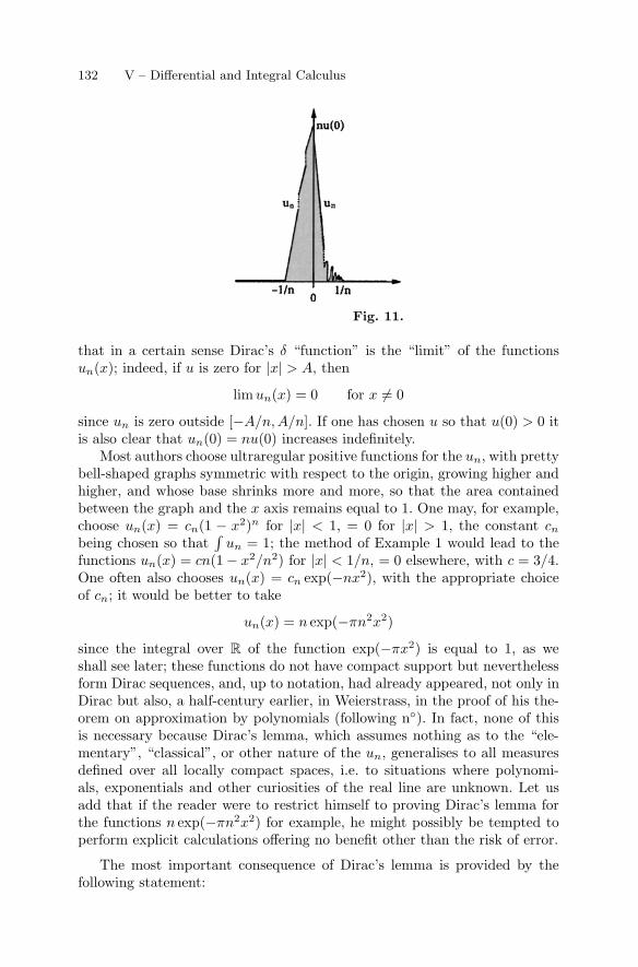
132 V – Differential and Integral Calculus
Fig. 11.
that in a certain sense Dirac’s δ “function” is the “limit” of the functionsun(x); indeed, if u is zero for |x| > A, then
limun(x) = 0 for x �= 0
since un is zero outside [−A/n,A/n]. If one has chosen u so that u(0) > 0 itis also clear that un(0) = nu(0) increases indefinitely.
Most authors choose ultraregular positive functions for the un, with prettybell-shaped graphs symmetric with respect to the origin, growing higher andhigher, and whose base shrinks more and more, so that the area containedbetween the graph and the x axis remains equal to 1. One may, for example,choose un(x) = cn(1 − x2)n for |x| < 1, = 0 for |x| > 1, the constant cn
being chosen so that∫
un = 1; the method of Example 1 would lead to thefunctions un(x) = cn(1 − x2/n2) for |x| < 1/n, = 0 elsewhere, with c = 3/4.One often also chooses un(x) = cn exp(−nx2), with the appropriate choiceof cn; it would be better to take
un(x) = n exp(−πn2x2)
since the integral over R of the function exp(−πx2) is equal to 1, as weshall see later; these functions do not have compact support but neverthelessform Dirac sequences, and, up to notation, had already appeared, not only inDirac but also, a half-century earlier, in Weierstrass, in the proof of his the-orem on approximation by polynomials (following n◦). In fact, none of thisis necessary because Dirac’s lemma, which assumes nothing as to the “ele-mentary”, “classical”, or other nature of the un, generalises to all measuresdefined over all locally compact spaces, i.e. to situations where polynomi-als, exponentials and other curiosities of the real line are unknown. Let usadd that if the reader were to restrict himself to proving Dirac’s lemma forthe functions n exp(−πn2x2) for example, he might possibly be tempted toperform explicit calculations offering no benefit other than the risk of error.
The most important consequence of Dirac’s lemma is provided by thefollowing statement:
§ 8. Approximation Theorems 133
Theorem 26. Let (un) be a Dirac sequence. For every function f definedand continuous on R one has
f(x) = lim∫
f(x − y)un(y)dy(27.8)
uniformly on every compact subset of R if f is bounded or just if the un
vanish outside the same compact set.
To establish (8) for f bounded it is enough to apply the lemma to thefunction y → f(x−y). The little calculation in Dirac’s lemma shows moreoverthat ∣∣∣∣f(x)
∫un(y)dy −
∫f(x − y)un(y)dy
∣∣∣∣ ≤(27.9)
≤∫
|f(x) − f(x − y)| |un(y)| dy
and since the integral of un tends to 1, we reduce to proving that the righthand side converges uniformly to 0 when x remains in a compact subset Kof R.
Take an ε > 0. Since f is uniformly continuous on every compact K in Rthere is an r > 0 such that |f(x − y) − f(x)| ≤ ε for x ∈ K and |y| ≤ r. Byvirtue of property (D 4) of Dirac sequences, the contribution of the interval|y| ≤ r is thus ≤ Mε for any n and x ∈ K.
For such a choice of r the contribution of the set |y| ≥ r to the right handside of (9) is less than the product of 2‖f‖ by the integral of |un| extendedover |y| ≥ r; for n large it is therefore < ε for any x ∈ R, by (D 3).
Finally one obtains an estimate for (9) valid for all the x ∈ K simultane-ously, whence the theorem in this case.
If the un are all zero for |y| ≥ A, the first part of the argument survivesunchanged. In the second, one remarks that the contribution of the set |y| ≥ ris in fact an integral over r ≤ |y| ≤ A; if x remains in the compact |x| ≤ B,the integral (9) involves only the pairs (x, y) satisfying |x| ≤ B, |y| ≤ A + B,a set on which the difference |f(x) − f(x − y)| is bounded, which allows oneto conclude as in the preceding case.
The interest of Theorem 26 is that it allows one to approximate the func-tion f by C∞ functions, or even polynomials, much more “regular” thanitself. The idea had already been met in 1926 chez the American NorbertWiener, the future inventor of “cybernetics”, whom Dirac no doubt had notread.
In the first case, one remarks for a start, that thanks to the function
u(x) = exp(−1/x) for x > 0, = 0 for x ≤ 0,
which is C∞ on R as we saw a long time ago, there are “many” C∞ func-tions of compact support54 on R: to obtain one it suffices to multiply a C∞
54 Recall that the “support” of a function f is the smallest closed set outside whichit is zero, i.e. the closure of the set {f �= 0}.
134 V – Differential and Integral Calculus
function vanishing for x < a by a C∞ function zero vanishing for x > b. Theset of these functions is a vector space which, since Schwartz, has been de-noted D(R) or simply D. There are clearly even positive C∞ functions, zerooutside arbitrarily given intervals; on dividing by their integral over R onemay assume that the integral is equal to 1. Thus there exist Dirac sequencesformed of functions ϕn ∈ D. Using the function u(x) above, one may forexample take ϕn(x) = cnu(x + 1/n)u(1/n − x) with a constant cn such that∫
ϕn(x)dx = 1.The functions (8) which, for every continuous function f on R, converge
to f , are then C∞, as we shall see. It all amounts to showing that for everyϕ ∈ D zero for |x| ≥ A and every continuous function f , the convolutionproduct
f � ϕ(x) =∫
f(x − y)ϕ(y)dy =∫ A
−A
f(x − y)ϕ(y)dy(27.10)
is C∞; this is the method of regularising an “arbitrary” function; it evenprovides a C∞ result for every regulated function f on R.
We remark that the change of variable x − y = t transforms (10) into
f � ϕ(x) =∫
f(t)ϕ(x − t)dt =∫
ϕ(x − t)f(t)dt = ϕ � f(x)(27.10’)
(one has dy = −dt, but the integral changes orientation and the factor −1 iseliminated on reestablishing the natural orientation). To check that the inte-gral is a C∞ function of x one may restrict to a compact interval J = [−A,A].Since ϕ(x−t) is zero for |x−t| ≥ B, because ϕ is of compact support, the inte-gral (10’) is, for every x ∈ J , extended over the interval K = [−A−B, A+B].We are then in the situation of Theorem 9 of n◦ 9: the function ϕ(x−t) playsthe role of the function f(x, y) of the theorem and f(t) that of µ.
The convolution product is therefore differentiable, so, returning to (10’),
(f � ϕ)′ = f � ϕ′ or D(f � ϕ) = f � Dϕ.(27.11)
Since the derivative Dϕ of a function in D is again in D, one may iterate(11), which leads to the general relation
(f � ϕ)(n) = f � ϕ(n) or Dn(f � ϕ) = f � Dnϕ(27.12)
hypothesising only that f is regulated on R. It is not the differentiability orthe continuity of f which matters, it is that of ϕ.
Theorem 27. For every function f defined and continuous on R there existsa sequence fn of C∞ functions which converges to f uniformly on everycompact subset of R. If f is of compact support one may assume that the fn
are zero outside a fixed compact set.
§ 8. Approximation Theorems 135
Obvious: one applies Theorem 26 to a Dirac sequence formed by functionsof D, bearing in mind what we want to establish. If f is zero for |x| > A andif one assumes, for example, that the ϕn vanish for |x| ≥ 1/n, it is clear thatthe fn are all zero for |x| ≥ A + 1, qed.
If the function f is C1, one can, in formula (10), differentiate directlywith respect to x, again thanks to Theorem 9 of n◦ 9, which shows that
D(f � ϕ) = Df � ϕ(27.13)
in this case. Replacing ϕ by the ϕn ∈ D of a Dirac sequence one sees thatthe Dfn converge to Df uniformly on every compact set. Therefore:
Corollary. Let f be a function of class Cp (p ≤ +∞) on R. There exists asequence fn of C∞ functions such that
lim f (r)n (x) = f (r)(x)
uniformly on every compact for every finite r ≤ p.
All these results extend, with the same proofs, to functions defined onRp.
28 – Approximation by polynomials
We shall now prove Weierstrass’ theorem on the uniform approximation ofcontinuous functions by polynomials on a compact set. The proof we shallgive of this – Weierstrass’, up to a few details – also uses approximation byconvolution products.
(i) We start from a function u which is positive, integrable, has integral 1over R, but is not zero for |x| large because we shall choose for u an every-where convergent power series. For every function f(x) which is continuouson R and zero for |x| ≥ A given, we put
fn(x) = n
∫f(y)u(nx − ny)dy.(28.1)
These functions being the convolution products of f by the functionsun(x) = nu(nx), which form a Dirac sequence, the fn converge to f uni-formly on every compact set.
(ii) We assume that u(x) =∑
apxp is the sum of a power series that
converges for every x ∈ C; then
fn(x) = n
∫f(y)dy
∑p
apnp(x − y)p.
For x and n given, the power series in x − y converges normally on everycompact set, and in particular on the interval |y| ≤ A outside which f(y) = 0.Since f is bounded we may integrate term-by-term, whence
136 V – Differential and Integral Calculus
fn(x) =∑
p
napnp
∫(x − y)pf(y)dy =
∑fn,p(x),(28.2)
where we integrate over |y| ≤ A. For |x| ≤ A we have |x − y| ≤ 2A, whence
|fn,p(x)| ≤ 2An‖f‖.|ap|(2nA)p,(28.3)
the factor 2A coming from the integration over |y| < A. Since the powerseries u(x) converges for any x, so for example at the point 2nA, the righthand side of (3) is the general term of a convergent series. The series (2)therefore converges normally on |x| ≤ A.
(iii) The general term of the series (2) is a polynomial in x, as we seeon expanding (x − y)p. Since it converges normally on |x| ≤ A, its partialsums converge to fn uniformly on this interval. Since the fn converge tof uniformly in |x| ≤ A, by (i), we can, replacing them by partial sums ofsufficiently high order, obtain a sequence of polynomials converging to funiformly on |x| ≤ A.
(iv) We still have to show the existence of u. The functionu(x) = c. exp(−πx2) meets the requirements. It is clearly positive, integrable,has total integral 1 for c suitably chosen (c = 1, in fact) and is expandableas an everywhere convergent power series.
Theorem 28 (Weierstrass, 1885). Let f be a real function defined andcontinuous on a compact interval K ⊂ R. Then there exists a sequence ofpolynomials which converges to f uniformly on K.
It is enough to observe that f can be extended to a continuous functionon all R, zero for |x| large: complete the graph of f by linear functions.
For a function f defined and continuous on all R, or, more generally, onan unbounded interval I, it is impossible to find a sequence of polynomialspn which converges uniformly to f on I except in the trivial case where fis itself a polynomial (Chap. III, n◦ 5, end). As we then noted, it is alwayspossible to demand that the pn should converge to f uniformly on everycompact K ⊂ I.
If the interval I is bounded but not compact, we have seen in n◦ 8, asa consequence of Corollary 2 of the uniform continuity theorem, that ap-proximation by polynomials is possible only if f is uniformly continuous onI; f then extends to be a continuous function on the compact interval ob-tained by adjoining the endpoints to I, and Weierstrass’ theorem applied tothis compact interval yields the result. In short, Weierstrass’ theorem is bestpossible. Having said this, there are more difficult approximation theorems,where, instead of considering polynomials, one considers for example, lin-ear combinations of exponential functions exp(anx) with given an (suitablychosen . . . ).
Up to details, the proof of Weierstrass’ theorem which we have presentedis that of Weierstrass himself; his aim was to show that, though it is certainlyimpossible to represent every continuous function by simple analytic formulae
§ 8. Approximation Theorems 137
(algebraic, power series, etc.), it is however possible to find series of simplefunctions – as it happens, polynomials and not only monomials – whichrepresent them.
There are many other proofs of the theorem; Hairer and Wanner, Analysisby Its History, p. 264, cited a dozen (from G. Meinardus, 1964), the latestdating from 1934. This leads me to suspect, without having checked, thatperhaps one should add to their list the one and only model proof, applicablein the much more general framework of compact topological spaces, namelythe Stone-Weierstrass theorem, a generalisation obtained in the 1930s by aChicago mathematician who notably wrote in this period the first system-atic exposition of the theory of “abstract” Hilbert spaces; he did much after1945 to invite or recruit foreign mathematicians – I benefitted in 1950 – andmoreover had a pronounced taste for gastronomy in general and French inparticular; this was a good sign in an American, but one has to say that hewas the son of a Chief Justice of the Supreme Court and not of a corn farmerfrom the Bible Belt. The theorem is as follows. Assume given on a compactspace X, (Appendix to Chap. III, n◦ 7) a set A – the initial letter of theword “algebra” – of continuous functions with complex values satisfying thefollowing conditions:
(a) the complex constants are in A;(b) the sum and the product of two functions of A are again in A;(c) for every f ∈ A, the complex conjugate function f is in A;(d) for any distinct points x, y ∈ X there exists an f ∈ A such that
f(x) �= f(y).
Then every continuous function on X is the uniform limit on X of a sequenceof functions fn ∈ A. For a proof with hardly any calculations, see Dieudonne,Vol. 1, Chap. VII, n◦ 3, or Serge Lang, Analysis I (Addison-Wesley, 1968),Chap. VIII, n◦ 5. If X is a compact subset of C, one may take for A the set ofpolynomials in x and y [but not just the polynomials in z: they do not satisfycondition (c), without mentioning the fact that, in an open subset of C, auniform limit of polynomials in z is holomorphic, as we shall see], whenceWeierstrass’ theorem for two variables, or for p variables on taking X in Rp.
In particular let us take for X the circle |z| = 1, the set of complexnumbers of the form z = e2πit with t ∈ R defined modulo Z. A function fdefined and continuous on X is transformed into a function g(t) = f(e2πit)defined, continuous and of period 1 on R, and vice-versa as is easy to see –one has only to check continuity. On X, a polynomial in x = (z + z)/2 andy = (z − z)/2i, i.e. in z and z, clearly reduces to a finite sum of the form∑
ane2πint with the n ∈ Z, in other words to a trigonometric polynomial(Chap. III, n◦ 5). Corollary: every function defined, continuous and peri-odic on R is the uniform limit of trigonometric polynomials, as announced inChap. III, n◦ 5. This is the result on which one may base the whole theoryof Fourier series. One may also, we shall see this in the chapter dedicated tothe subject, prove it by explicit elementary calculations, as did Weierstrass
138 V – Differential and Integral Calculus
himself. But Stone’s method applies to generalisations of Fourier series (har-monic analysis on compact groups for example) where direct and explicitcalculations would be impossible. Moreover, in this way one has no need ofprovidential functions like exp(−πx2).
This kind of “nonconstructive” proof naturally does not satisfy the calcu-lators. There is a proof with calculations in Hairer and Wanner, pp. 264–268,and, moreover, the graphs showing the approximations they provide.
29 – Functions having given derivatives at a point
To end this section with a nonobvious theoretical exercise we shall prove thefollowing result55:
Theorem 29 (Emile Borel, 1895). For every sequence (an) of complexnumbers there exists an indefinitely differentiable function f of compact sup-port on R such that f (n)(0) = an for every n ∈ N.
Our first move, faced by this theorem, is to put
f(x) =∑
anxn/n!(29.1)
in accordance with Maclaurin’s formula. Bad idea: the series has every chanceof diverging for x �= 0.
All the same, (1) contains the germ of an idea for a proof. The functionanxn/n! = anx[n] has the virtue that, at the origin, all its derivatives are zeroexcept for the n-th, which is equal to an. We shall replace it by a functionfn ∈ D, the space of C∞ functions of compact support on R, possessingthe same properties but making the series converge. And since we will haveto calculate the successive derivatives of the series it will be necessary todifferentiate it term-by-term, i.e. to apply Theorem 20 of Chap. III, n◦ 17.In other words, the function f will be given by the formula
f(x) =∑
fn(x)(29.2)
where the fn ∈ D satisfy, for example,
fn(x) = 0 for |x| ≥ 1(29.3)
to yield a result of compact support, satisfy also55 The proof which follows (H. Mirkil, 1956) develops the one that one finds for ex-
ample in Lars Hormander, The Analysis of Linear Partial Differential Operators(Vol. 1, Springer-Verlag, 1983, p. 16), where it takes sixteen lines. Borel’s com-plete result is much stronger but requires difficult results on analytic functions:one may assume f to be of class C∞ on a neighbourhood of 0 and real-analyticapart from at the origin. See Remmert, Funktionentheorie II, p. 237.
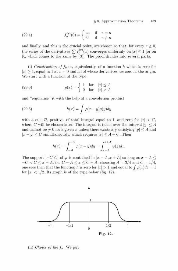
§ 8. Approximation Theorems 139
f (r)n (0) =
{an if r = n0 if r �= n
(29.4)
and finally, and this is the crucial point, are chosen so that, for every r ≥ 0,the series of the derivatives
∑f
(r)n (x) converges uniformly on |x| ≤ 1 [or on
R, which comes to the same by (3)]. The proof divides into several parts.
(i) Construction of f0 or, equivalently, of a function h which is zero for|x| ≥ 1, equal to 1 at x = 0 and all of whose derivatives are zero at the origin.We start with a function of the type
g(x) ={
1 for |x| ≤ A0 for |x| > A
(29.5)
and “regularise” it with the help of a convolution product
h(x) =∫
ϕ(x − y)g(y)dy(29.6)
with a ϕ ∈ D, positive, of total integral equal to 1, and zero for |x| > C,where C will be chosen later. The integral is taken over the interval |y| ≤ Aand cannot be �= 0 for a given x unless there exists a y satisfying |y| ≤ A and|x − y| ≤ C simultaneously, which requires |x| ≤ A + C. Then
h(x) =∫ +A
−A
ϕ(x − y)dy =∫ x+A
x−A
ϕ(z)dz.
The support [−C, C] of ϕ is contained in [x − A, x + A] so long as x − A ≤−C < C ≤ x + A, i.e. C − A ≤ x ≤ C + A; choosing A = 3/4 and C = 1/4,one sees then that the function h is zero for |x| > 1 and equal to
∫ϕ(z)dz = 1
for |x| < 1/2. Its graph is of the type below (fig. 12).
Fig. 12.
(ii) Choice of the fn. We put
140 V – Differential and Integral Calculus
fn(x) = h(bnx)anx[n].(29.7)
with the bn > 0 to be chosen later. Since we want the fn to be zero for|x| ≥ 1, it is prudent to impose the condition
bn > 1(29.8)
on them. Let us calculate the derivatives of the fn at the origin. They areobtained from Leibniz’ formula: (fg)[r] =
∑f [r−p]g[p]. At x = 0 all the
derivatives of x[n] are zero except the n-th, equal to 1. Those of h(bnx) are allzero at the origin starting from the first. The derivative of order r of fn cannotbe �= 0 unless there exists a p such that p = n and p = r simultaneously, inother words if r = n. In this case, there remains f
(n)n (0) = an, so that the fn
do satisfy condition (4), and this whatever the bn.(iii) Convergence of the series
∑f
(r)n (x). We shall show that one may
choose the bn so that
|f (r)n (x)| ≤ 1/2n for every x, every r, and every n > r,(29.9)
the sole significance of the numbers 1/2n being that they form a convergentseries. As this is the case, it is clear that the series
∑fn(x) will be normally
convergent as will be all the derived series, the sum of the series will thereforebe in D and its derivatives, calculated by differentiating the series term-by-term, will be the an at the origin, by the relations (4).
It remains to choose the bn. By (7) and Leibniz, we have
f (r)n (x) =
∑?h(r−p)(bnx)br−p
n anx[n−p](29.10)
with numerical coefficients denoted ? and whose exact values are of littleimportance. Since h(bnx) = 0 for |x| > 1/bn, it suffices, to evaluate theresult, to work on the interval |x| ≤ 1/bn, which allows us to estimate themonomials appearing in (10). In this interval we have |br−p
n xn−p| ≤ br−nn , an
expression independent of p, whence, passing to the uniform norms,∥∥∥f (r)n
∥∥∥ ≤ br−nn |an|
∑?∥∥∥h(r−p)
∥∥∥ = Mr,nbr−nn ≤ Mr,n/bn(29.11)
for r < n. Since, for n given, the conditions (9) to be satisfied involve only ther < n, so are finite in number, it then suffices, to satisfy them simultaneously,to choose Mr,n/bn ≤ 1/2n for every r < n, i.e.
bn ≥ max0≤r<n
2nMr,n,
qed.This proof is typical of the current techniques in analysis. All the work
consists of rigorously controlling the orders of magnitude of the numbers orfunctions that one is manipulating. Nothing is calculated explicitly. We areat the antipodes of the analysis of the Founders.
§ 9. Radon measures in R or C 141
§ 9. Radon measures in R or C
30 – Radon measures on a compact set
As we have already observed on several occasions, many of the results ofintegration theory use only a few quasi-algebraic properties of the integralm(f) of a function: linearity, positivity and continuity with respect to uniformconvergence, in other words, Theorem 1 of n◦ 2.
We have also observed on occasion that there are curious analogies be-tween integrals and series. Let us work on a compact interval of R and con-sider, for example, the two following situations:
(i) Theorem 9 of n◦ 9 and Theorem 24 of n◦ 25 which allow one to calculatethe derivative of a “continuous” sum
ϕ(y) =∫
f(x, y)µ(x)dx(30.1)
of functions by the formula
ϕ′(y) =∫
D2f(x, y)µ(x)dx,(30.2)
(ii) Theorem 19 of Chap. III, n◦ 17 which, translated into the languageof series, allows one to differentiate a “discrete” sum
ϕ(y) =∑
fn(y)(30.3)
of functions by the formula
ϕ′(y) =∑
f ′n(y).(30.4)
The analogy would be even clearer if, starting from a finite or denumerableset D of points of R, a scalar function µ(ξ) on D satisfying
∑ |µ(ξ)| < +∞,and a function f(ξ, y) defined on D × Y , one put
ϕ(y) =∑
f(ξ, y)µ(ξ)(30.3’)
when one would have
ϕ′(y) =∑
D2f(ξ, y)µ(ξ)(30.4’)
of course under suitable hypotheses as in the case (i).One may unify the two cases formally by writing, for every reasonable
function f of a “continuous” or “discrete” variable, µ(f) =∫
f(x)µ(x)dxin the first case and µ(f) =
∑f(ξ)µ(ξ) in the second; using the notation
fy(x) = f(x, y) one then has
ϕ(y) = µ(fy) and ϕ′(y) = µ [(D2f)y]
142 V – Differential and Integral Calculus
in both cases.We are led to introduce, in a general way, functions f → µ(f) in which
the variable f is a more or less arbitrary function on a given interval X (ora metric space, or even, in the “abstract” theory of integration, an arbitraryset) possessing properties formally analogous to those of integrals and series.Clearly one has to impose some restrictions on the category of functions fconsidered: it is not possible to define the expression
∫f(x)dx in a natural
way for every function f on R. On the other hand, the problem, whetherdealing with series or integrals, has always been the following: one is givenµ(f) for particularly simple functions f (finite sums in the discrete case, stepfunctions in the continuous case) and one hopes to extend the constructionin a natural way to more complicated functions (series in the discrete case,integrals of regulated or semicontinuous functions, or even more general inthe Lebesgue theory, in the case of continuous sums).
In the simplest case, of a compact interval K ⊂ R, the constructions inn◦ 1 and 2 of this Chapter led us to associate to each step function ϕ a num-ber µ(ϕ) possessing the following properties:
(i) linearity: µ(αϕ + βψ) = αµ(ϕ) + βµ(ψ) for any constants α and βand step functions ϕ and ψ;
(ii) continuity with respect to uniform convergence: there exists a constantM(µ) ≥ 0 such that
|µ(ϕ)| ≤ M(µ)‖ϕ‖K(30.5)
for any ϕ. If, for every interval I ⊂ K, we write χI for the function equal to1 on I and to 0 in K − I, we may then associate a “measure”
µ(I) = µ(χI)
to I, which manifestly has the additivity property (M 2) of n◦ 1:
I = I1 ∪ . . . ∪ In =⇒ µ(I) = µ(I1) + . . . + µ(In)
if the Ik are pairwise disjoint, because χI is then the sum of the characteristicfunctions of the Ik. From this one can calculate the integral µ(ϕ) of everystep function using a finite partition of K into intervals Ik on which ϕ isconstant; on choosing points ξk ∈ Ik, one has
µ(ϕ) =∑
ϕ(ξk)µ(Ik)
sinceϕ(x) =
∑ϕ(ξk)χIk
(x)
for every x ∈ K, whence the formula by the linearity of ϕ → µ(ϕ).
§ 9. Radon measures in R or C 143
Starting from this data one may then define µ(f) for every regulatedfunction f on K by passing to uniform limits: if the step functions ϕn convergeuniformly to f then the relation (5), which implies
|µ(ϕp) − µ(ϕq)| ≤ M(µ)‖ϕp − ϕq‖K ,
shows that the integrals µ(ϕn) form a Cauchy sequence, so converge; the limitdepends only on f since, if (ψn) is another uniform approximation to f , therelation (5) shows that µ(ϕn)−µ(ψn) tends to 0. (Compare the constructionof the real numbers starting from Cauchy sequences of rational numbers.)Whence µ(f), with, quite clearly, the two usual properties of linearity andcontinuity:
|µ(f)| ≤ M(µ)‖f‖K .
Note in passing that this construction, which does not involve the “lower”and “upper” integrals of n◦ 1, but applies – no big deal! – only to regulatedfunctions, does not use the hypothesis of positivity of µ, namely that
ϕ ≥ 0 =⇒ µ(ϕ) ≥ 0.(30.6)
If this is satisfied then the relation ϕ ≤ ψ implies µ(ϕ) ≤ µ(ψ) and all thearguments of n◦ 1 concerning the lower and upper integrals of a bounded func-tion apply unchanged. As we have observed since n◦ 1, the three conditionsimposed on our functions µ(I) would be satisfied if one put µ(I) = µ(v)−µ(u)for I = (u, v), where µ(x) is an increasing function on K. Note also that thisconstruction mingles the discrete and the continuous sums: for example, put
µ(ϕ) =∫
K
ϕ(x)µ(x)dx +∑
ϕ(ξ)c(ξ)
where one integrates over K and where∑ |c(ξ)| < +∞; if ϕ is the charac-
teristic function of an interval I ⊂ K of any type, one finds clearly
µ(I) =∫
I
µ(x)dx +∑ξ∈I
c(ξ).
Physically, this comes down to considering that one has, on the one hand, adistribution of masses on K whose density in the usual sense (the ratio of themass of an “infinitely small” segment of K to its length) is given by the regu-lated function µ(x) and, on the other hand, a countable set of “point” massesc(ξ). One also meets this kind of situation in the most modern physics: in thespectrum of the radiation emitted by the Sun, there are “bands”, whose inten-sity is a continuous function of the frequency, and “lines” which concentratea nonzero intensity on an interval consisting of a single frequency. Nothingvery artificial here; Newton would have said that one meets this in Nature . . .
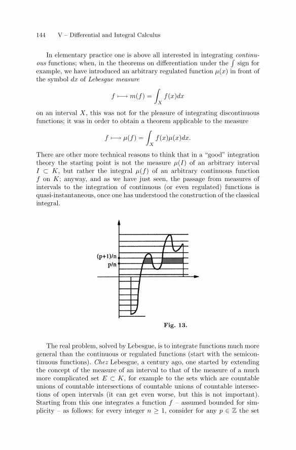
144 V – Differential and Integral Calculus
In elementary practice one is above all interested in integrating continu-ous functions; when, in the theorems on differentiation under the
∫sign for
example, we have introduced an arbitrary regulated function µ(x) in front ofthe symbol dx of Lebesgue measure
f −→ m(f) =∫
X
f(x)dx
on an interval X, this was not for the pleasure of integrating discontinuousfunctions; it was in order to obtain a theorem applicable to the measure
f −→ µ(f) =∫
X
f(x)µ(x)dx.
There are other more technical reasons to think that in a “good” integrationtheory the starting point is not the measure µ(I) of an arbitrary intervalI ⊂ K, but rather the integral µ(f) of an arbitrary continuous functionf on K; anyway, and as we have just seen, the passage from measures ofintervals to the integration of continuous (or even regulated) functions isquasi-instantaneous, once one has understood the construction of the classicalintegral.
Fig. 13.
The real problem, solved by Lebesgue, is to integrate functions much moregeneral than the continuous or regulated functions (start with the semicon-tinuous functions). Chez Lebesgue, a century ago, one started by extendingthe concept of the measure of an interval to that of the measure of a muchmore complicated set E ⊂ K, for example to the sets which are countableunions of countable intersections of countable unions of countable intersec-tions of open intervals (it can get even worse, but this is not important).Starting from this one integrates a function f – assumed bounded for sim-plicity – as follows: for every integer n ≥ 1, consider for any p ∈ Z the set
§ 9. Radon measures in R or C 145
En,p = {p/n ≤ f(x) < p/n + 1/n} on which f is equal to p/n to within 1/n;these sets form a finite partition of K; if they belong to the category of thosefor which one can define m(E) [or µ(E) in the case of an arbitrary measure],one may consider the Lebesgue sum,
∑p m(Ep,n)p/n (as against the Riemann
sum); geometrically, one considers the set of the points (x, y) in the plane ly-ing between K and the graph of f , cuts it by the lines y = p/n into horizontalslices having the Ep,n as bases, and approximates the required area
∫f(x)dx
by the sum of the areas of these horizontal slices (fig. 13). Lebesgue’s geniuswas not just to have replaced the decomposition into vertical slices by decom-position into horizontal slices; it was to have understood that this innocentmodification of the traditional procedure provided a method formidably morepowerful than that of Riemann. It has been generalised ad libitum, but noone has ever progressed in a way that would be useful beyond certain ad hocproblems. The mode of exposition has only been modified from that chosenby Lebesgue in an age when the concepts of vector space, of linear form andof norm had not yet been isolated: analysis had been arithmetised and wasnow, in Germany rather more than in France, as rigorous as number theory,but it had not yet been algebraised; in fact, integration theory was probablythe impetus that forced the analysts to learn, even to invent, what a vectorspace of infinite dimension ought to be, starting with Hilbert spaces.
Since, for every compact set K ⊂ C (or in Rp, or for every metric compactspace), one has available the space56 L(K) = C0(K) of the scalar continuousfunctions on K and the norm
‖f‖K = sup |f(x)|of uniform convergence on K, one is led to define a Radon measure on K inthe following way: it is a map
µ : L(K) −→ C
which is linear in the general sense of algebra and continuous in the generalsense of the theory of normed vector spaces: there exists a constant M(µ)such that
|µ(f)| ≤ M(µ)‖f‖K
for every f ∈ L(K). Such a measure is said to be positive if
f ≥ 0 =⇒ µ(f) ≥ 0.
One shows without much difficulty (Chap. XI, n◦ 17, Theorem 29) that everymeasure µ can be put in the form µ(f) = µ1(f)−µ2(f)+iµ3(f)−iµ4(f) with56 The notation L(X) was introduced in Andre Weil, L’integration dans les groupes
topologiques et ses applications (Paris, Hermann, 1940), a book from which manyof my generation learned integration and generalised Fourier analysis. I assumethat Weil chose it not only in homage to Lebesgue, but also because he composeddirectly onto the typewriter . . .
146 V – Differential and Integral Calculus
positive measures µk. It is generally worth restricting oneself – or reducing– to the case of positive measures, by far the most important, and the onlyones for which a grand theory has been constructed.
Leibniz’ notation having amply proved its usefulness, one imitates it bywriting
µ(f) =∫
K
f(x)dµ(x),
a notation which will justify itself better below, but which one may usewithout understanding its origin. So, by definition, we have the relation∫
K
(3 sin x − 5 log x) dµ(x) = 3∫
K
sin x dµ(x) − 5∫
K
log x dµ(x)(30.7)
for any constants 3 and −5 and continuous functions sin and log on K, alsothat ∣∣∣∣
∫K
f(x)dµ(x)∣∣∣∣ ≤ M(µ)‖f‖K(30.8)
for every continuous function f on K, with a constant M(µ) to be chosenas small as possible; this is the norm of the measure µ, notation ‖µ‖; for theusual measure m on an interval of R, we have ‖m‖ = m(K). The object of thiscondition is to guarantee that Theorem 4 concerning uniform limits appliesagain here: if a sequence of continuous functions fn converges uniformly onK to a necessarily continuous limit f one has
|µ(f) − µ(fn)| = |µ(f − fn)| ≤ M(µ)‖f − fn‖K ,(30.9)
whence µ(f) = limµ(fn). If, likewise, a series s(x) =∑
un(x) of continuousfunctions on K converges normally, one may integrate term-by-term:
µ(∑
un
)=∑
µ(un).(30.10)
In short, we have transformed Theorems 1 and 4 of § 1 into definitions.
Example 1. Choose a function µ(x), integrable (in the usual sense) on aninterval K ⊂ R, and put
µ(f) =∫
f(x)µ(x)dx(30.11)
for every f ∈ L(K). Linearity is obvious and continuity follows from theinequalities
|µ(f)| ≤∫
|f(x)|.|µ(x)|dx ≤ ‖f‖K .
∫|µ(x)|dx.
Here ‖µ‖ ≤ ∫ |µ(x)|dx (and, in fact, we have equality).
§ 9. Radon measures in R or C 147
The simplest case is obtained by choosing µ(x) = 1; this is the measurem which appears in all of classical analysis and has been the subject ofthis chapter. It is called the Lebesgue measure on K, not, of course, becausepoor Henri Lebesgue had discovered that the length of an interval (a, b) isequal to b − a, but because it is for this particularly important measurethat he invented the grand integration theory that was later extended to allmeasures defined on all reasonable topological spaces. In the general case (11)one speaks of the measure of density µ(x) with respect to Lebesgue measure:obvious physical interpretation.
Example 2. Choose a countable set D of points of K and, for every ξ ∈ D, anumber c(ξ) ∈ C; assuming
∑ |c(ξ)| < +∞ one may define
µ(f) =∑
c(ξ)f(ξ)(30.12)
for every continuous function f on K, the series being taken over D. Nohypothesis on the compact set K is necessary here.
Example 3. Take K = A×B where A and B are compact intervals in R andput
m(f) =∫∫A×B
f(x, y)dxdy
for every continuous function f on K (n◦ 9, Theorem 10).
Example 4. Choose for K the set T : |z| = 1 of complex numbers of modulus 1(unit circle); the “parametric representation” z = exp(2πit) = e(t) of thepoints of T transforms any function f ∈ L(T) into a continuous functionf [e(t)] of period 1 on R. One thus obtains a very privileged measure on T byputting
m(f) =∫ 1
0
f [e(t)]dt =12π
∫ 2π
0
f(eit)dt(30.13)
for every f ∈ L(T); this is what dominates the theory of Fourier series. Onecould clearly replace T by any other parametrised curve, but it is better todefer this type of example to when we shall need it (mainly line integrals ofholomorphic functions).
We shall see later how, in the case of an interval, one may construct allthe measures on K by a procedure analogous to that of n◦ 1 and 2 concerningLebesgue measure.
We shall now show quickly how some of the theorems on Lebesgue mea-sure extend to Radon measures.
Differentiation under the∫
sign. Theorem 9 of n◦ 9 extends trivially (i.e.with the same proof) to the functions
148 V – Differential and Integral Calculus
g(y) =∫
f(x, y)dµ(x),(30.14)
where we have not indicated that the integral is extended over K; f is acontinuous function on K×J and J an interval of R. The result is a continuousfunction and it is of class C1 if D2f exists and is continuous, with, in thiscase,
g′(y) =∫
D2f(x, y)dµ(x).(30.15)
To reproduce the proofs verbatim here would be to waste our time and thatof the reader. The simplest case is that of an interval K ⊂ R, but in fact theargument and the result apply to every compact set K if one knows that,on every compact set (for example, here, K × H where H ⊂ J is a compactinterval), a continuous function is uniformly continuous.
Exercise. The function f � µ(x) =∫
f(x − y)dµ(y) is C∞ if f is C∞ andof compact support on R.
Double integrals. A slightly less easy exercise consists of generalising The-orem 10 to measures:
Theorem 30. Let K and H ⊂ R be two compact sets, µ and ν measures onK and H, and f a continuous function on K × H. Then∫
K
dµ(x)∫
H
f(x, y)dν(y) =∫
H
dν(y)∫
K
f(x, y)dµ(x).(30.16)
Inspired by the proof of Theorem 10 one is led, for a given r > 0, to takepartitions (Kp) of K and (Hq) of H, and to compare each member of (16) tothe sum of the analogous expressions obtained on replacing K and H by Kp
and Hq, i.e. by multiplying f(x, y) by χp(x)θq(y) where χp and θq are thecharacteristic functions of Kp and Hq. Since∑
χp(x) = 1 on K,∑
θq(y) = 1 on H,(30.17)
we have f(x, y) =∑
f(x, y)χp(x)θq(y) on K × H, which explains why thesum of the integrals over the products Kp×Hq is the integral of f over K×H.
This method is not directly applicable here: for an arbitrary measure wedon’t yet know how to integrate discontinuous functions. The solution is toreplace the discontinuous functions which frustrate us by continuous positivefunctions kp and hq on K and H still satisfying (17) and zero outside setsAp or Bq which are small enough that the function f is constant to within ron each product Ap ×Bq. By (17) and the linearity of µ and ν, we will thenhave ∫
dµ(x)∫
f(x, y)dν(y) =(30.18)
=∑∫
dµ(x)∫
f(x, y)kp(x)hq(y)dν(y),
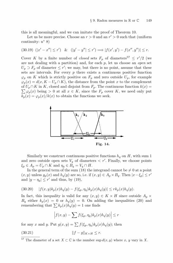
§ 9. Radon measures in R or C 149
this is all meaningful, and we can imitate the proof of Theorem 10.Let us be more precise. Choose an r > 0 and an r′ > 0 such that (uniform
continuity: n◦ 8)
(|x′ − x′′| ≤ r′) & (|y′ − y′′| ≤ r′) =⇒ |f(x′, y′) − f(x′′, y′′)| ≤ r.(30.19)
Cover K by a finite number of closed sets Fp of diameters57 ≤ r′/2 (weare not dealing with a partition) and, for each p, let us choose an open setUp ⊃ Fp of diameter ≤ r′; we may, but there is no point, assume that thesesets are intervals. For every p there exists a continuous positive functionϕp on K which is strictly positive on Fp and zero outside Up, for exampleϕp(x) = d(x,K −Up ∩K), the distance from the point x to the complementof Up ∩K in K, closed and disjoint from Fp. The continuous function k(x) =∑
ϕp(x) being > 0 at all x ∈ K, since the Fp cover K, we need only putkp(x) = ϕp(x)/k(x) to obtain the functions we seek.
Fig. 14.
Similarly we construct continuous positive functions hq on H, with sum 1and zero outside open sets Vq of diameters < r′. Finally, we choose pointsξp ∈ Ap = Up ∩ K and ηq ∈ Bq = Vq ∩ H.
In the general term of the sum (18) the integrand cannot be �= 0 at a point(x, y) unless gp(x) and hq(y) are so, i.e. if (x, y) ∈ Ap×Bq. Then |x−ξp| ≤ r′
and |y − ηq| ≤ r′ and thus, by (19),
|f(x, y)kp(x)hq(y) − f(ξp, ηq)kp(x)hq(y)| ≤ rkp(x)hq(y).(30.20)
In fact, this inequality is valid for any (x, y) ∈ K × H since outside Ap ×Bq either kp(x) = 0 or hq(y) = 0. On adding the inequalities (20) andremembering that
∑kp(x)hq(y) = 1 one finds∣∣∣f(x, y) −
∑f(ξp, ηq)kp(x)hq(y)
∣∣∣ ≤ r
for any x and y. Put g(x, y) =∑
f(ξp, ηq)kp(x)hq(y); then
‖f − g‖K×H ≤ r.(30.21)57 The diameter of a set X ⊂ C is the number sup d(x, y) where x, y vary in X.
150 V – Differential and Integral Calculus
Denote the two sides of (16) by λ′(f) and λ′′(f). These are measureson K × H: linearity is obvious, and continuity follows from |λ′(f)| ≤M(µ)M(ν)‖f‖K×H , with the same inequality for λ′′. By (21), we then haveλ′(f) = λ′(g) and λ′′(f) = λ′′(g) to within M(µ)M(ν)r. Since r > 0 isarbitrary it is then enough to show that λ′(g) = λ′′(g) to establish (16).
But this is obvious: for any k ∈ L(K) and h ∈ L(H) we have∫dµ(x)∫
k(x)h(y)dν(y) =∫
dµ(x)k(x)∫
h(y)dν(y) =
=∫
dµ(x)k(x)ν(h) = ν(h)∫
k(x)dµ(x) = µ(k)ν(h)
and the same calculation, with the same result, on interchanging the orderof the integrations; since g is a linear combination of functions of the formk(x)h(y) we have λ′(g) = λ′′(g), qed.
This proof generalises fully: in every metric space one may find systemsof continuous positive functions satisfying (17) and zero outside arbitrarilysmall given open sets; such systems of functions are called partitions of unity.The method applies to triple, quadruple, integrals etc.
The two essential points in the proof are that (i) the identity (16) isobvious if f(x, y) is a finite sum of functions of the form g(x)h(y), (ii) everyf ∈ L(K×H) is, by (21), the limit of such functions, uniformly on K×H. Thegeneral Stone-Weierstrass theorem provides (ii) without the least calculation:it is enough to check that the set A of functions of the form
∑gp(x)hq(y),
with gp ∈ L(K) and hq ∈ L(H) complex-valued, satisfies the conditions (a),(b), (c), (d) of n◦ 28; a very easy exercise.
Finally one has to observe that the map
f −→ λ(f) =∫ ∫
f(x, y)dµ(x)dν(y)
– it is now unnecessary to specify the order of the integrations – is a mea-sure on the compact set K × H, the product measure or Cartesian productof µ and ν. On choosing dµ(x) = dx and dν(y) = dy one recovers Lebesguemeasure in the plane.
All the theory expounded in n◦s 10 and 11 extends to general positivemeasures, with the very same proofs: we have established what we need andonly have to replace m(f) everywhere by µ(f) and m(K) by M(µ) or ‖µ‖.
31 – Measures on a locally compact set
Since Lebesgue measure allows one to integrate over intervals which are nei-ther compact nor even bounded we should be able to extend the definition of
§ 9. Radon measures in R or C 151
Radon measures to this case. First we examine the classical situation moreclosely, it being a little less simple than the compact case.
If X = (a, b) ⊂ R is an arbitrary interval one cannot define the integral∫f(x)dx over X for just any continuous function f on X: there must be
convergence conditions at the endpoints of X if these do not belong to X orare infinite. A radical method to eliminate them is to assume the functionf(x) to be zero when x is close enough to a or b, i.e. that there exists acompact58 interval K = [u, v] ⊂ X such that f(x) = 0 for x /∈ K. Then∫
K′f(x)dx =
∫K
f(x)dx for K ⊂ K ′ ⊂ X,(31.1)
so that the integral taken over X converges absolutely for a trivial reasonand reduces to the integral over any compact set outside which f is zero.The functions of this kind are called of compact support on X (n◦ 27); theset of these is a vector space which we again denote by L(X) and which manyother authors denote C0
c (X), with a suffix c whose significance is obvious. Forevery compact K ⊂ X the set of f ∈ L(X) which vanish outside K is a vectorsubspace L(X,K) of L(X).
In this way Lebesgue measure on X gives us a (positive) linear formf → m(f) on L(X). We have a norm on L(X)
‖f‖X = supx∈X
|f(x)|,(31.2)
but if X is not bounded the linear form m is not continuous relative to thisnorm, in other words, there is no finite constant M such that
|m(f)| =∣∣∣∣∫ v
u
f(x)dx
∣∣∣∣ ≤ M. supx∈X
|f(x)| = M‖f‖X(31.3)
for every continuous function f on X which is zero outside some compactinterval K = [u, v] ⊂ X and otherwise arbitrary. For example take X =]0,+∞[, with 0 < u < v < +∞; you can clearly find a function f withvalues everywhere between 0 and 1, equal to 1 on K and zero outside acompact K ′ ⊂ X a little larger than K (make the characteristic function ofK continuous by replacing its discontinuities at u and v by line segments); forsuch a function the left hand side of the preceding inequality is > m(K) =v − u and the right hand side is equal to M ; impossible if u and v can takearbitrary values between 0 and +∞. For X = [0,+∞[, one may take u = 0,but the difficulty remains.
Failing (3), one may all the same observe that
58 If a is finite one must have a ≤ u if a ∈ X, a < u if not; if b is finite similarlyone must have b ≥ v if b ∈ X, b > v if not. In the case where a or b is infiniteboth u and v must be finite. If for example X = [0, +∞[, a continuous functionon X is so in particular at 0, so that the only difficulty in integrating it over Xcomes from the other endpoint of X.
152 V – Differential and Integral Calculus
|m(f)| ≤ m(K)‖f‖X for every f ∈ L(X,K)(31.4)
since in fact the integral over X involves only the compact K ⊂ X off whichf is zero. This is the result we can generalise.
We shall call a Radon measure on X any linear form µ on the vector spaceL(X) having the following property: for every compact K ⊂ X there existsa constant MK(µ) such that
|µ(f)| ≤ MK(µ)‖f‖X(31.5)
for every f ∈ L(X,K). In other words, we assume that the linear form µis continuous on each subspace L(X,K), though not necessarily on all ofL(X) =
⋃L(X,K).
Example 1. Take for X the open interval ]0,+∞[ and
µ(f) =∫ +∞
0
f(x)dx/x.(31.6)
There is no problem with convergence for f ∈ L(X) since f(x) is zero on aneighbourhood of 0 and for x large. If f is zero outside K = [u, v] then
|µ(f)| ≤ (log v − log u)‖f‖X ,
whence continuity.One could clearly replace the function 1/x by any regulated function p
on X; if the function p is absolutely integrable in X then
|µ(f)| ≤ M(µ)‖f‖X
where M(µ) =∫ |p(x)|dx no longer depends on the support K of f . In this
particular case the linear form µ is continuous on L(X) and not just on thesubspaces L(X,K). A measure possessing this property is said to be boundedor of finite total mass on X.
Example 2. If one replaces the open interval ]0,+∞[ by the closed interval[0,+∞[ the formula (6) is no longer meaningful, since, in this case, a functionf ∈ L(X) is required to be zero for x large but not on a neighbourhood of 0,so allowing every chance of making the integral (6) divergent.
But one can replace 1/x by a function that poses no problem at the origin,and, for example, put
µ(f) =∫ +∞
0
f(x)xsdx with Re(s) > −1.(31.7)
If f is zero outside K = [0, v] then
|µ(f)| ≤ MK(µ)‖f‖X
§ 9. Radon measures in R or C 153
with
MK(µ) =∫ v
0
|xs|dx =vRe(s)+1
Re(s) + 1.
One obtains a bounded measure on replacing xs by an absolutely integrablefunction on X, for example xse−x with Re(s) > −1.
Example 3. Choose a compact interval K ⊂ X, a measure µ on K and con-sider the linear form f → ∫ f(x)dµ(x), where one integrates over K, soinvolving only the values of f on this fixed compact set. This example showsthat a measure on K may also be considered as a measure on X: all the massis supported by K.
Example 4. For X = R put
µ(f) =∑
f(n),(31.8)
summing over Z. If f is zero outside a compact K, only the n ∈ K count,whence |µ(f)| ≤ MK(µ)‖f‖X where MK(µ) is the number of integers in K.
More generally one may put
µ(f) =∑
c(ξ)f(ξ)(31.9)
assuming only that for every compact K ⊂ X the series taken over the ξ ∈ Kconverges absolutely. Then, for f ∈ L(X,K),
|µ(f)| ≤ MK(µ)‖f‖X where MK(µ) =∑ξ∈K
|c(ξ)|
since the ξ /∈ K do not appear in (9). If the total series∑ |c(ξ)| converges
one obtains a bounded measure as in Example 2, for example
µ(f) =∑
n−2 sin(1/n)f(1/n) for X = [0,+∞[, where one sums over theintegers > 0.
In all this, the fact that X is an interval of R hardly plays a role. Onecould assume that X is a locally compact subset of C (end of n◦ 23) – an openset, a closed set, or, the general case, the intersection of an open and of aclosed59 set – and consider the vector space L(X) of continuous functions onX which are zero outside some compact subset of X, with its obvious vectorsubspaces L(X,K). A Radon measure on X is then again a linear form onL(X) whose restriction to each L(X,K) satisfies a relation (5).
The assumption that X is locally compact is needed to assure the exis-tence of “many” functions f ∈ L(X). The proof rests on the following lemma:59 Exercise. Show from the definition that the intersection of two locally compact
subsets of C is locally compact.
154 V – Differential and Integral Calculus
Lemma. Let X be a subset of C, K a compact subset of X and F a subsetof X disjoint from K and closed in60 X. There exists a continuous functionf on X such that
f = 1 on K, 0 ≤ f < 1 on X − K, f = 0 on F.(31.10)
If X is locally compact one may assume f ∈ L(X).
Consider the function d(x,K); it is continuous, zero on K and > 0 outsideK. Let us show that there exists an r > 0 such that d(x,K) ≥ r for everyx ∈ F . If not, there exist points xn ∈ F and yn ∈ K such that d(xn, yn)tends to 0. Since K is compact, one can (Bolzano-Weierstrass) assume thatyn tends to a limit b ∈ K ⊂ X; it is clear that then the xn ∈ F tend to b.But since F is closed in X this implies b ∈ F ∩ K = ∅, absurd.
This done, we put f(x) = ϕ[d(x,K)] with a function ϕ(t) defined andcontinuous for t ≥ 0. For f to satisfy the conditions (10) it is enough that ϕshould satisfy the following conditions: (i) ϕ(0) = 1; (ii) 0 ≤ ϕ(t) < 1 for anyt > 0; (iii) ϕ(t) = 0 for t ≥ r. The existence of such functions is clear.
Now assume X locally compact. Since F is closed in X for every a ∈ X−Fthere exists an open ball BX(a) of X [the set of x ∈ X such that d(a, x) < r]such that the corresponding closed ball BX(a) [the set of x ∈ X such thatd(a, x) ≤ r] does not meet F . Since X is locally compact one may assumeBX(a) compact by choosing r small enough. Since K is also compact onemay (Borel-Lebesgue) cover it with a finite number of balls BX(ap) [theseare the intersections of X with open balls of C]. The union U of these balls isopen in X and contained in the compact union H of the BX(ap), which doesnot meet F . If one applies the lemma to K and X −U ⊃ X −H one obtainsa function f which satisfies (10) and is zero outside the compact subset H ofX, qed.
Exercise – Let X be the (not locally compact) union of the open disc|z| < 1 and of the interval [1, 2] of R. Show that f(1) = 0 for every functionf continuous in X and zero outside a compact K ⊂ X.
Examples of measures on a locally compact subset of C are not always asobvious as in R. Certainly there are discrete measures like those of Example 4of n◦ 31. It is easy to obtain measures analogous to those of Examples 1 and2 if X is open: choose an arbitrary continuous function ρ on X (for we donot yet know how to integrate anything else) and put
µ(f) =∫ ∫
f(x, y)ρ(x, y)dxdy
for every f ∈ L(X); for every compact K ⊂ X the set X − K is open in Cso that on agreeing to attribute to f(x, y)ρ(x, y) the value 0 outside X one60 This means that every limit in X of points of F is in F , or again, that F is the
intersection of X and of a closed set in C. This is the general concept of closedset in the metric space obtained by endowing the set X with its usual distance.
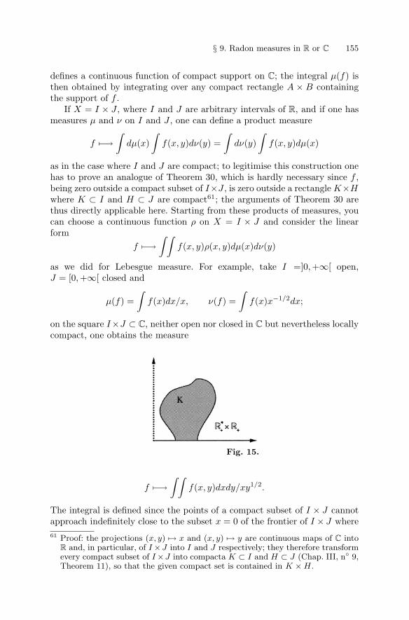
§ 9. Radon measures in R or C 155
defines a continuous function of compact support on C; the integral µ(f) isthen obtained by integrating over any compact rectangle A × B containingthe support of f .
If X = I × J , where I and J are arbitrary intervals of R, and if one hasmeasures µ and ν on I and J , one can define a product measure
f −→∫
dµ(x)∫
f(x, y)dν(y) =∫
dν(y)∫
f(x, y)dµ(x)
as in the case where I and J are compact; to legitimise this construction onehas to prove an analogue of Theorem 30, which is hardly necessary since f ,being zero outside a compact subset of I×J , is zero outside a rectangle K×Hwhere K ⊂ I and H ⊂ J are compact61; the arguments of Theorem 30 arethus directly applicable here. Starting from these products of measures, youcan choose a continuous function ρ on X = I × J and consider the linearform
f −→∫ ∫
f(x, y)ρ(x, y)dµ(x)dν(y)
as we did for Lebesgue measure. For example, take I =]0,+∞[ open,J = [0,+∞[ closed and
µ(f) =∫
f(x)dx/x, ν(f) =∫
f(x)x−1/2dx;
on the square I×J ⊂ C, neither open nor closed in C but nevertheless locallycompact, one obtains the measure
Fig. 15.
f −→∫ ∫
f(x, y)dxdy/xy1/2.
The integral is defined since the points of a compact subset of I × J cannotapproach indefinitely close to the subset x = 0 of the frontier of I × J where61 Proof: the projections (x, y) �→ x and (x, y) �→ y are continuous maps of C into
R and, in particular, of I ×J into I and J respectively; they therefore transformevery compact subset of I ×J into compacta K ⊂ I and H ⊂ J (Chap. III, n◦ 9,Theorem 11), so that the given compact set is contained in K × H.
156 V – Differential and Integral Calculus
the integration in x would diverge. In particular, a compact subset remainsseparated from the point (0, 0), which does not belong to I × J .
Exercise (less easy). Choose X = C and try to define a measure on X bythe formula
µ(f) =∫ ∫
f(x, y) (x2 + y2)−s dxdy;
find the real values of s for which this is meaningful.
The integration of semicontinuous functions in the case of a noncompactinterval X, more generally of a locally compact subset of C, proceeds moreor less as in the compact case. Dini’s Theorem shows that if an increasingsequence of continuous functions fn has a continuous function f for its upperenvelope, then convergence is uniform on every compact K ⊂ X. As in thecase where X is compact, one deduces that if f and the fn are in L(X) thenµ(f) = limµ(fn) = supµ(fn) for every positive measure µ on X.
On replacing the fn by fn − f1, so replacing f by f − f1 and µ(fn) byµ(fn) − µ(f1), we may assume the fn positive. Since they are majorised byf they are all zero outside a compact K of X independent of n. Thus
|µ(f) − µ(fn)| ≤ MK(µ)‖f − fn‖X ,
which yields the result, clearly applicable to increasing philtres as in n◦ 10.To pass from this to the lsc functions we shall restrict ourselves to func-
tions ϕ which are positive outside a compact K ⊂ X for otherwise one cannothope that L(X) contains an f ≤ ϕ. Being lsc, such a function is boundedbelow on the compact set K = {ϕ ≤ 0} [n◦ 10, (vi)], whence the existence ofa f0 ∈ L(X) majorised by62 ϕ. If one writes Linf(ϕ) for the set of f ∈ L(X)satisfying f ≤ ϕ one sees, as in n◦ 10, on considering ϕ− f0 which is lsc andpositive, that ϕ is the upper envelope of the f ∈ Linf(ϕ): in the case of anarbitrary locally compact X ⊂ C, the lemma above, applied taking for K theset {a} and for F the set of x ∈ X such that d(a, x) ≥ r, replaces the figureof n◦ 10. Then one puts
µ∗(ϕ) = supf∈Linf(ϕ)
µ(f).(31.11)
The crucial point, as in n◦ 10, is that one may calculate µ∗(ϕ) using anyincreasing philtre Φ ⊂ Linf(ϕ) having ϕ for upper envelope. First, the sup ofthe µ(f) for f ∈ Φ is clearly ≤ µ∗(ϕ). Oppositely, for every h ∈ Linf(ϕ) the setof functions inf(f, h), where f ∈ Φ, is an increasing philtre (obvious) whoseupper envelope is h (obvious); the version of Dini’s Theorem just obtainedthen shows that µ(h) is the upper bound of the integrals of the inf(f, h);
62 Let −m, m ≥ 0, be the minimum of ϕ on K, i.e. on X. By the lemma abovethere exists an f ≥ 0 in L(X) which is equal to m on K. The function −f is theone we need.
§ 9. Radon measures in R or C 157
since inf(f, h) ≤ f we conclude that the upper bound of the µ(f), f ∈ Φ,majorises µ(h) for every h ∈ Linf(ϕ), so majorises µ∗(ϕ), whence the result.
From here, the machine turns on its own and yields the three properties(i), (ii) and (iii) of n◦ 11. No need to reproduce the proofs: you replace m byµ and Cinf by Linf .
One may also consider on X the usc functions ψ which are lower envelopesof continuous functions of compact support; this assumes these ψ negativeoutside a compact (so zero outside a compact if they are positive everywhere),and since they are bounded above on it, the existence in L(X) of functionswhich majorise it is obvious as in the other case. Writing Lsup(ψ) for the setof f ∈ L(X) which majorise ψ, one denotes by µ∗(ψ) the lower bound of theµ(f) when f runs through Lsup(ψ). Replacing ψ by −ψ would bring us backto the previous case.
These constructions apply in particular to the everywhere continuousfunctions on X. Such a function ϕ is, in many ways, the difference of twopositive continuous functions ϕ′ and ϕ′′, for example ϕ+ and ϕ−, to whichthe definition of the integral of an lsc function applies. It is therefore nat-ural to define µ(ϕ) = µ(ϕ′) − µ(ϕ′′), but the definition has no meaning ifµ(ϕ′) = µ(ϕ′′) = +∞, and depends a priori on the choice of ϕ′ and ϕ′′. Toeliminate the first objection one limits oneself to integrable continuous func-tions for µ (understood: absolutely) for which one may choose ϕ′ and ϕ′′ tohave finite integrals; since 0 ≤ ϕ+ ≤ ϕ′ we have the same for ϕ+ and ϕ−, sothat |ϕ| = ϕ+ + ϕ− is also integrable. The second objection is not one: for
ϕ′′ − ϕ′ = ψ′′ − ψ′ =⇒ ϕ′′ + ψ′ = ψ′′ + ϕ′,
whence the result thanks to the additivity of the integral.In the case of Lebesgue measure on an interval X we recover the defini-
tions of n◦ 22. We may restrict ourselves to the case of a positive continuousfunction ϕ. N◦ 22 defines convergence of the integral
∫ϕ(x)dx by insisting
that the integrals on the compact sets K ⊂ X be bounded above; here weassume that the integrals of the functions f ∈ L(X) majorised by ϕ arebounded above. Since each of these f is zero outside a compact of X it isclear that convergence in the sense of n◦ 22 implies convergence in the presentsense. Moreover, it is clear, since ϕ is continuous, that, for every compact in-terval K ⊂ X, there exists an f ∈ L(X) equal to ϕ on K and ≤ ϕ everywhereelsewhere: multiply ϕ by a continuous function of compact support with val-ues in [0, 1] and equal to 1 on K. Whence the implication in the reverse sense,and the equality of the integrals of ϕ on X defined by the two methods.
32 – The Stieltjes construction
Returning to the case of R, let us take an increasing function µ(x) (in thewide sense) on X = (a, b) and show how, in generalising the definition ofthe usual integral, one may associate with it a measure on X which we shall
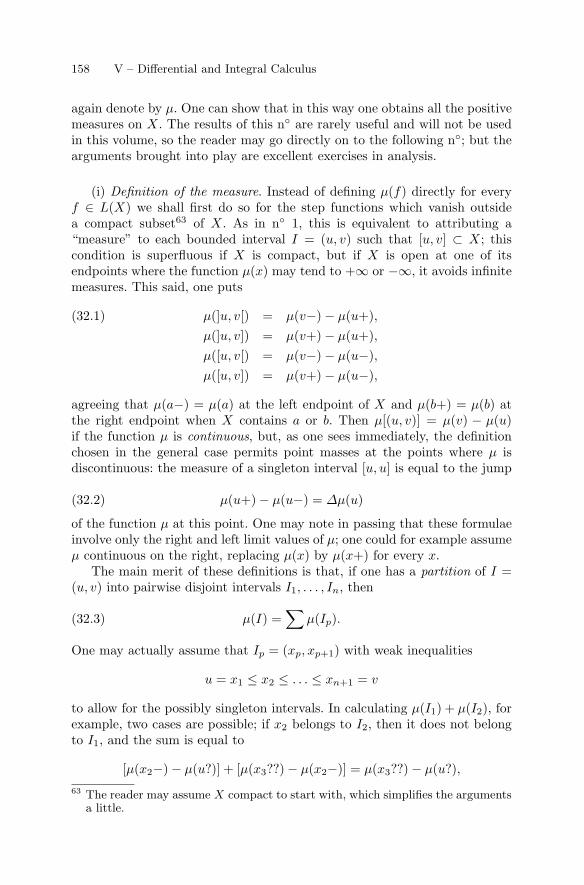
158 V – Differential and Integral Calculus
again denote by µ. One can show that in this way one obtains all the positivemeasures on X. The results of this n◦ are rarely useful and will not be usedin this volume, so the reader may go directly on to the following n◦; but thearguments brought into play are excellent exercises in analysis.
(i) Definition of the measure. Instead of defining µ(f) directly for everyf ∈ L(X) we shall first do so for the step functions which vanish outsidea compact subset63 of X. As in n◦ 1, this is equivalent to attributing a“measure” to each bounded interval I = (u, v) such that [u, v] ⊂ X; thiscondition is superfluous if X is compact, but if X is open at one of itsendpoints where the function µ(x) may tend to +∞ or −∞, it avoids infinitemeasures. This said, one puts
µ(]u, v[) = µ(v−) − µ(u+),(32.1)µ(]u, v]) = µ(v+) − µ(u+),µ([u, v[) = µ(v−) − µ(u−),µ([u, v]) = µ(v+) − µ(u−),
agreeing that µ(a−) = µ(a) at the left endpoint of X and µ(b+) = µ(b) atthe right endpoint when X contains a or b. Then µ[(u, v)] = µ(v) − µ(u)if the function µ is continuous, but, as one sees immediately, the definitionchosen in the general case permits point masses at the points where µ isdiscontinuous: the measure of a singleton interval [u, u] is equal to the jump
µ(u+) − µ(u−) = ∆µ(u)(32.2)
of the function µ at this point. One may note in passing that these formulaeinvolve only the right and left limit values of µ; one could for example assumeµ continuous on the right, replacing µ(x) by µ(x+) for every x.
The main merit of these definitions is that, if one has a partition of I =(u, v) into pairwise disjoint intervals I1, . . . , In, then
µ(I) =∑
µ(Ip).(32.3)
One may actually assume that Ip = (xp, xp+1) with weak inequalities
u = x1 ≤ x2 ≤ . . . ≤ xn+1 = v
to allow for the possibly singleton intervals. In calculating µ(I1) + µ(I2), forexample, two cases are possible; if x2 belongs to I2, then it does not belongto I1, and the sum is equal to
[µ(x2−) − µ(u?)] + [µ(x3??) − µ(x2−)] = µ(x3??) − µ(u?),
63 The reader may assume X compact to start with, which simplifies the argumentsa little.
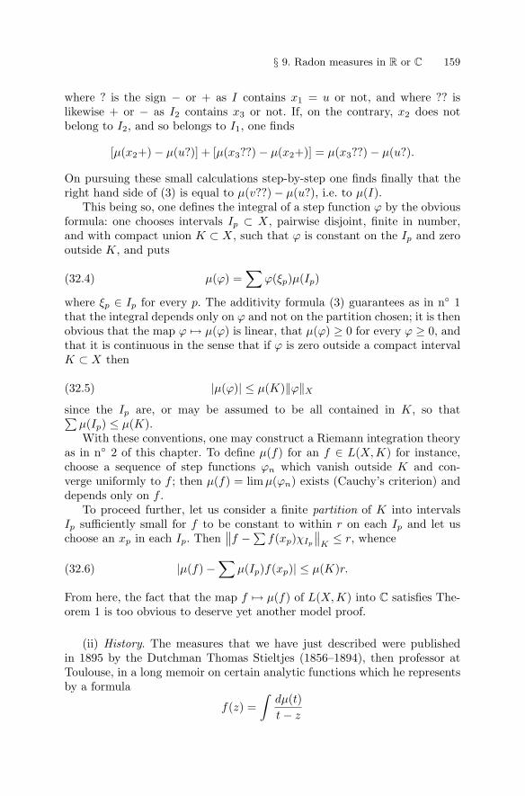
§ 9. Radon measures in R or C 159
where ? is the sign − or + as I contains x1 = u or not, and where ?? islikewise + or − as I2 contains x3 or not. If, on the contrary, x2 does notbelong to I2, and so belongs to I1, one finds
[µ(x2+) − µ(u?)] + [µ(x3??) − µ(x2+)] = µ(x3??) − µ(u?).
On pursuing these small calculations step-by-step one finds finally that theright hand side of (3) is equal to µ(v??) − µ(u?), i.e. to µ(I).
This being so, one defines the integral of a step function ϕ by the obviousformula: one chooses intervals Ip ⊂ X, pairwise disjoint, finite in number,and with compact union K ⊂ X, such that ϕ is constant on the Ip and zerooutside K, and puts
µ(ϕ) =∑
ϕ(ξp)µ(Ip)(32.4)
where ξp ∈ Ip for every p. The additivity formula (3) guarantees as in n◦ 1that the integral depends only on ϕ and not on the partition chosen; it is thenobvious that the map ϕ → µ(ϕ) is linear, that µ(ϕ) ≥ 0 for every ϕ ≥ 0, andthat it is continuous in the sense that if ϕ is zero outside a compact intervalK ⊂ X then
|µ(ϕ)| ≤ µ(K)‖ϕ‖X(32.5)
since the Ip are, or may be assumed to be all contained in K, so that∑µ(Ip) ≤ µ(K).With these conventions, one may construct a Riemann integration theory
as in n◦ 2 of this chapter. To define µ(f) for an f ∈ L(X,K) for instance,choose a sequence of step functions ϕn which vanish outside K and con-verge uniformly to f ; then µ(f) = limµ(ϕn) exists (Cauchy’s criterion) anddepends only on f .
To proceed further, let us consider a finite partition of K into intervalsIp sufficiently small for f to be constant to within r on each Ip and let uschoose an xp in each Ip. Then
∥∥f −∑ f(xp)χIp
∥∥K
≤ r, whence
|µ(f) −∑
µ(Ip)f(xp)| ≤ µ(K)r.(32.6)
From here, the fact that the map f → µ(f) of L(X,K) into C satisfies The-orem 1 is too obvious to deserve yet another model proof.
(ii) History. The measures that we have just described were publishedin 1895 by the Dutchman Thomas Stieltjes (1856–1894), then professor atToulouse, in a long memoir on certain analytic functions which he representsby a formula
f(z) =∫
dµ(t)t − z
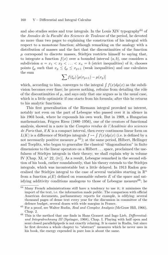
160 V – Differential and Integral Calculus
and also studies series and true integrals. In the Louis XIV typography64 ofthe Annales de la Faculte des Sciences de Toulouse of the period, he devotedno more than two pages to explaining the construction of his integral withrespect to a monotone function; although remarking on the analogy with adistribution of masses and the fact that the discontinuities of the functionµ correspond to discrete masses, Stieltjes restricts himself to saying that,to integrate a function f(x) over a bounded interval (a, b), one considers asubdivision a = x1 < x2 < . . . < xn = b (strict inequalities) of it, choosespoints ξp such that xp ≤ ξp ≤ xp+1 (weak inequalities) and one calculatesthe sum ∑
f(ξp) [µ(xp+1) − µ(xp)]
which, according to him, converges to the integral∫
f(x)dµ(x) as the subdi-vision becomes ever finer; he proves nothing, refrains from detailing the roleof the discontinuities of µ, and says only that one argues as in the usual case,which is a little optimistic if one starts from his formula; after this he returnsto his analytic functions.
This first generalisation of the Riemann integral provoked no interest,notably not even on the part of Lebesgue who passed over it in silence inhis 1903 book, where he expounds his own work. But in 1909, a Hungarianmathematician, Frigyes Riesz (1880–1956), one of the creators of functionalanalysis, showed in a note in the Comptes rendus de l’Academie des sciencesde Paris that, if K is a compact interval, then every continuous linear form onL(K) is a difference of Stieltjes integrals f → ∫ f(x)dµ(x) (i.e. is defined by anot necessarily positive measure µ 65); at the same period, Hilbert, Hellingerand Toeplitz, who began to generalise the classical “diagonalisation” in finitedimensions to the linear operators on a Hilbert . . . space, proclaimed the use-fulness of Stieltjes integrals in their theory; we shall explain why in volumeIV [Chap. XI, n◦ 22, (iv)]. As a result, Lebesgue remarked in the second edi-tion of his book, rather roundaboutly, that his theory extends to the Stieltjesintegrals, which was incontestable but a little delayed. In 1913 Radon gen-eralised the Stieltjes integral to the case of several variables starting in Rn
from a function µ(E) defined on reasonable subsets E of the space and sat-isfying additivity conditions analogous to those of Lebesgue measure66; he64 Many French administrations still have a tendency to use it; it minimises the
import of the text, i.e. the information made public. The comparison with officialAmerican documents, parliamentary reports for example, is edifying: severalthousand pages of dense text every year for the discussion in committee of thedefence budget, several dozen with wide margins in France.
65 For a proof, see Walter Rudin, Real and Complex Analysis (McGraw Hill, 1966),Chap. 2.
66 This is the method that one finds in Hans Grauert and Ingo Lieb, Differential-und Integralrechnung III (Springer, 1968), Chap. I. Playing with half open andsemi closed parallelipipeds is not exactly relaxing. It is easier in Rudin, but sincehe first devotes a whole chapter to “abstract” measures which he never uses inhis book, the energy expended in pure loss is about the same.
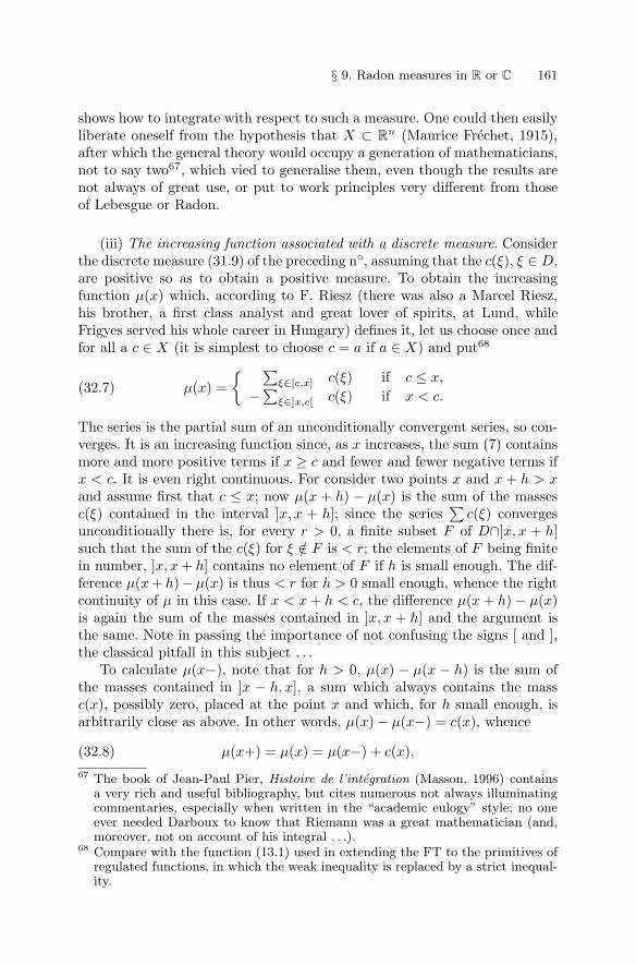
§ 9. Radon measures in R or C 161
shows how to integrate with respect to such a measure. One could then easilyliberate oneself from the hypothesis that X ⊂ Rn (Maurice Frechet, 1915),after which the general theory would occupy a generation of mathematicians,not to say two67, which vied to generalise them, even though the results arenot always of great use, or put to work principles very different from thoseof Lebesgue or Radon.
(iii) The increasing function associated with a discrete measure. Considerthe discrete measure (31.9) of the preceding n◦, assuming that the c(ξ), ξ ∈ D,are positive so as to obtain a positive measure. To obtain the increasingfunction µ(x) which, according to F. Riesz (there was also a Marcel Riesz,his brother, a first class analyst and great lover of spirits, at Lund, whileFrigyes served his whole career in Hungary) defines it, let us choose once andfor all a c ∈ X (it is simplest to choose c = a if a ∈ X) and put68
µ(x) ={ ∑
ξ∈[c,x] c(ξ) if c ≤ x,
−∑ξ∈]x,c[ c(ξ) if x < c.(32.7)
The series is the partial sum of an unconditionally convergent series, so con-verges. It is an increasing function since, as x increases, the sum (7) containsmore and more positive terms if x ≥ c and fewer and fewer negative terms ifx < c. It is even right continuous. For consider two points x and x + h > xand assume first that c ≤ x; now µ(x + h) − µ(x) is the sum of the massesc(ξ) contained in the interval ]x, x + h]; since the series
∑c(ξ) converges
unconditionally there is, for every r > 0, a finite subset F of D∩]x, x + h]such that the sum of the c(ξ) for ξ /∈ F is < r; the elements of F being finitein number, ]x, x + h] contains no element of F if h is small enough. The dif-ference µ(x + h)− µ(x) is thus < r for h > 0 small enough, whence the rightcontinuity of µ in this case. If x < x + h < c, the difference µ(x + h) − µ(x)is again the sum of the masses contained in ]x, x + h] and the argument isthe same. Note in passing the importance of not confusing the signs [ and ],the classical pitfall in this subject . . .
To calculate µ(x−), note that for h > 0, µ(x) − µ(x − h) is the sum ofthe masses contained in ]x − h, x], a sum which always contains the massc(x), possibly zero, placed at the point x and which, for h small enough, isarbitrarily close as above. In other words, µ(x) − µ(x−) = c(x), whence
µ(x+) = µ(x) = µ(x−) + c(x),(32.8)67 The book of Jean-Paul Pier, Histoire de l’integration (Masson, 1996) contains
a very rich and useful bibliography, but cites numerous not always illuminatingcommentaries, especially when written in the “academic eulogy” style; no oneever needed Darboux to know that Riemann was a great mathematician (and,moreover, not on account of his integral . . .).
68 Compare with the function (13.1) used in extending the FT to the primitives ofregulated functions, in which the weak inequality is replaced by a strict inequal-ity.
162 V – Differential and Integral Calculus
so that µ(x) has a discontinuity of amplitude ∆µ(ξ) = c(ξ) at each pointξ ∈ D and is continuous at the other points of I.
(Since the ξ might well be all the rational points of X, this shows inpassing that the increasing functions are not just those suggested by theusual naive sketches.)
This done, it remains to apply the definitions (1) and to check that onerecovers the formula
µ(I) =∑ξ∈I
c(ξ)(32.9)
for every bounded interval I = (u, v) such that [u, v] ⊂ X.Next we have to check that the integral of a function f ∈ L(X,K) is
well defined by formula (31.9) of the preceding n◦. For this, let us considera partition of K into intervals Ip on which f is constant to within r andapply the approximation (6); the only intervals which count are those whichcontain points of D and (9) shows that
µ(f) =∑
p
f(xp)∑ξ∈Ip
c(ξ)
to within µ(K)r. But for ξ ∈ Ip one has f(xp) = f(ξ) to within r; on replacingf(xp) by f(ξ) for all the ξ ∈ Ip in the preceding formula, one commits, foreach p, an error less than r times the sum of the c(ξ) for ξ ∈ Ip, so a totalerror less than µ(K)r. Since f is zero outside K we have
µ(f) =∑ξ∈D
c(ξ)f(ξ)(32.10)
to within 2µ(K) r, whence the equality since r > 0 is arbitrary.
(iv) The discrete and continuous components of a measure. The sums (9)appear again in the general case of an arbitrary increasing function µ whenone wants to make the role of the discontinuities of µ in calculating µ(f)more precise. Furthermore we shall see that as well as a “continuous sum”,as in the classical case, µ(f) includes a “discrete sum”, namely the sum
µd(f) =∑
∆µ(ξ)f(ξ)(32.11)
extended over all the discontinuities of the increasing function µ; recall that∆µ(ξ) = µ(ξ+) − µ(ξ−).
First note that the set D of these points of discontinuity is countable69
and that ∑ξ∈K
∆µ(ξ) ≤ µ(K)
69 This also results from the fact that a monotone function is regulated.
§ 9. Radon measures in R or C 163
for every compact K = [u, v] ⊂ X. To see this, one first remarks that thepartial sum extended over a finite subset F of D ∩ K is ≤ µ(K); for if oneorders the points ξ1 < . . . < ξn of F one has
µ(ξ1−) < µ(ξ1+) ≤ . . . ≤ µ(ξn−) < µ(ξn+);
the sum in question is thus majorised by µ(ξn+)−µ(ξ1−) and so by µ(v+)−µ(u−) = µ(K) since µ(x) is increasing. For every integer n ≥ 1, the ξ ∈ Kwhere µ(ξ) > 1/n are therefore finite in number, whence simultaneouslythe denumerability of D ∩ K, so of D since X is the union of a sequenceof compact sets; hence the desired inequality, which makes the series (11)absolutely convergent for every bounded function f vanishing outside K, sofor f ∈ L(X,K).
Now the expression (11) reenters the preceding framework (iii). One isthus led to associate to the expression (11), a discrete measure on X, thecorresponding increasing function (7), here with c(ξ) = ∆µ(ξ). Now assumeµ(x) right continuous, which we may, as we have seen above, and put
µ(x) = µd(x) + µc(x);(32.12)
we thus define a continuous function µc since µ and µd have the same pointsof discontinuity ξ ∈ D, are both right continuous, and have the same “jumps”at these points. The function µc is moreover increasing. To see this, we haveto check that, for x ≤ y, we have µ(x) − µd(x) ≤ µ(y) − µd(y), i.e.
µd(y) − µd(x) ≤ µ(y) − µ(x) = µ(y+) − µ(x+),
which, by (7), means that the sum of the jumps of the function µ at thepoints of the interval ]x, y] where it is discontinuous is less than its variationbetween x and y, which is clear as we saw in proving (8).
This done, the functions µ(x), µd(x) and µc(x) define Radon measures onX and it is obvious – use Riemann sums – that, for every continuous functionf ∈ L(X), one has
µ(f) = µd(f) + µc(f) = µc(f) +∑
∆µ(ξ)f(ξ).(32.13)
Since the function µc(x) is continuous, the formulae (1) simplify:
µc(I) = µc(v) − µc(u) if I = (u, v),(32.14)
whether I is open, or closed, or . . ., and it is vain, in the “Riemann sums”for µc, to allow for the nonexisting discontinuities of µc(x). The measure µd
provides the “discrete sum” and the measure µc the “continuous sum” towhich we alluded above.
The ideal case is where the function µc(x) is of class C1. The mean valuetheorem then shows that if I = (u, v)
164 V – Differential and Integral Calculus
µc(I) = µ′c(w)(v − u) = µ′
c(w)m(I)
for a w ∈ I, where m(I) is Euclidean length. The Riemann sum∑
µc(Ip)f(xp)relative to a sufficiently fine partition of K, and in which xp can be assumedequal to wp, becomes
∑f(wp)µ′
c(wp)m(Ip); on decorating this calculationwith the inevitable ε and δ and calling µ what we would call µc, one thenfinds that for every increasing function µ of class C1 (so continuous), onehas ∫
f(x)dµ(x) =∫
f(x)µ′(x)dx;(32.15)
in 1697, but not in 1997, Leibniz would have said to you: obvious sincedµ(x) = µ′(x)dx . . . But here like elsewhere, it is not the notation whichmakes the formula obvious; it the formula that explains the notation.
Consider for example on X =]0,+∞[ the measure
f −→∫
f(x)dx/x
where one integrates over X. It corresponds to the monotone function µ(x) =log x: this is of class C1 and has derivative 1/x, whence the result by (15).For this measure, the measure of an interval I = (u, v) with 0 < u < v < +∞is µ(v) − µ(u) = log(v/u). One could extend this argument to any positivecontinuous function p other than 1/x: the increasing function defining theRadon measure
f −→∫
f(x)p(x)dx
is any primitive P (x) of p; the measure P (v) − P (u) of an interval I is theintegral of p extended over I.
Exercise. Prove (15) assuming that µ(x) is a primitive of a regulatedfunction ≥ 0.
Finally we remark that there are much more complicated monotone func-tions than the preceding, and for which the nondiscrete component of thecorresponding integral
∫f(x)dµ(x) is not of the form
∫f(x)p(x)dx, even if
you permit “densities” p(x) that are Lebesgue integrable on every compactset (“singular” measures concentrated on sets of measure zero). The generaltheory of integration treats them exactly like the others.
33 – Application to double integrals
As we saw at the end of n◦ 9 and in n◦ 30, one may integrate any continuousfunction f(x, y) on a rectangle X×Y with respect to Lebesgue measure dxdyor, more generally, with respect to a product measure dµ(x)dν(y), where Xand Y are compact intervals, and even if X and Y are noncompact, providedthat f ∈ L(X×Y ). But to integrate over an arbitrary compact set K ⊂ X×Y– in other words, and by definition, to integrate the function equal to f on K
§ 9. Radon measures in R or C 165
and to 0 elsewhere over X × Y – is not as simple, unless one imposes ad hochypotheses on K as the physicists and engineers do, or, like a mathematicianof the last century, declares that “the possibility of inverting the integrationsrests on the obvious principle that a sum remains the same for any order inwhich one adds the parts70”. The end of n◦ 9 has demonstrated the difficultyof the general problem.
The first problem is to define an integral over a compact set K ⊂ X ×Y ,in other words to integrate the function ϕ equal to f on K and to 0 at theother points of X×Y . Most luckily, it is upper semicontinuous if f is positive.For, consider a point a ∈ X×Y . If a /∈ K, then ϕ(x) = 0 on a neighbourhoodof a in X × Y since K is closed, whence the continuity of ϕ at a. At a pointa ∈ K, since f is continuous on K, for every r > 0 there exists an open discB(a) such that ϕ(x) = f(x) < f(a)+r on K∩B(a); since ϕ(x) = 0 for x /∈ Kand f(a) ≥ 0, we have ϕ(x) < f(a)+r = ϕ(a)+r for every x ∈ B(a), whencethe result. If f is negative, the function ϕ is on the contrary lsc since it is thenegative of the usc function constructed starting from −f . If f changes sign,catastrophe: we do not know how to integrate a function which is neither lscnor usc. But one may always write f = f+ − f− and deal with f+ and f−,for lack of a less crude method.
In these circumstances, as much to generalise and establish the standardresult:
Theorem 31. Let X and Y be two intervals, µ and ν positive measureson X and Y , and λ the product measure on X × Y . Let ϕ be an lsc (resp.usc) function on X × Y which is71 the upper (resp. lower) envelope of thef ∈ L(X×Y ) which minorise (resp. majorise) it. Then we have the followingproperties:
(i) For every x ∈ X, the function y → ϕ(x, y) is lsc (resp. usc);(ii) the function
x −→∫
Y
ϕ(x, y)dν(y),(33.1)
with values > −∞ (resp. < +∞), is lsc (resp. usc);
(iii) we have
λ(ϕ) =∫
X
dµ(x)∫
Y
ϕ(x, y)dν(y),(33.2)
the two members being simultaneously finite or infinite;70 Joseph Bertrand in his Traite de calcul differentiel et integral (1870), cited by
Jean-Paul Pier, Histoire de l’integration (Masson, 1997), p. 104. Bertrand taughtanalysis at the Ecole polytechnique from 1856 to 1894, which indicates the ca-pacity for renewal of the institution at this period. There also, in parallel, wereCharles Hermite (1869–1876) and Camille Jordan (1876–1911), who introducedsome notions of set theory before 1900.
71 a condition always satisfied if X and Y are compact or if ϕ is positive (resp.negative), etc.
166 V – Differential and Integral Calculus
(iv) we may invert the order of the integrations in (2).
We shall examine the case of an usc function, the other being trivialto deduce from it: multiply the function by −1. As always, the two crucialpoints will be that (a) a lower envelope of continuous functions is usc; (b) onemay calculate the integral of an usc function from any decreasing philtre ofcontinuous functions having ϕ as lower envelope. It remains to combine thesetools with the definitions; there is nothing more to the very short proof.
That the function y → ϕ(x, y) = ϕx(y) is usc on Y for every x ∈ X maybe seen either by using the definition in terms of inequalities, or from thefact that ϕ is the lower envelope of the set Φ = Lsup(ϕ) of the functionsf ∈ L(X × Y ) which majorise it.
One may therefore integrate ϕx, the result being < +∞, though it canbe −∞ for an usc function. For x given, it is clear that the set of functionsfx(y) = f(x, y), where f ∈ Φ, is a decreasing philtre of continuous functionson Y whose lower envelope is ϕx. Thus
ν(ϕx) = inf ν(fx).(33.3)
Let us now put Ff (x) = ν(fx) =∫
f(x, y)dν(y) and Fϕ(x) = ν(ϕx). Sincethe f vary in a decreasing philtre, it is the same for the Ff , because
f ≤ g =⇒ fx ≤ gx =⇒ Ff (x) ≤ Fg(x)
since ν is positive. Now the functions Ff (x) = ν(fx) are continuous on Xbecause, f being in L(X × Y ), the fx are zero outside the same compactsubset of Y , which allows us to argue as in n◦ 9, Theorem 9. Since
Fϕ(x) = ν(ϕx) = inf ν(fx) = inf Ff (x),
one concludes both that Fϕ is usc – point (ii) of the statement – and that
µ(Fϕ) = inf µ(Ff ).(33.4)
But (4) can again be written∫dµ(x)∫
ϕ(x, y)dν(y) = inf∫
dµ(x)∫
f(x, y)dν(y) = inf λ(f)(33.5)
where the inf is relative to the f ∈ Φ. Since, in (5), f runs through the set off ∈ L(X ×Y ) which majorise ϕ, the right hand side of (5) is, by definition ofthe integral of an usc function, equal to the integral λ(ϕ) of ϕ with respectto λ. The relation (5) therefore establishes (2). Point (iv) of the statement isthen obvious, qed.
To complete the enunciation of Theorem 31, assume that the function ϕis lsc, positive and integrable on X × Y , i.e., that λ(ϕ) < +∞. By (2) wethen have
§ 9. Radon measures in R or C 167
∫X
dµ(x)∫
Y
ϕ(x, y)dν(y) < +∞;
adopting the notation of the proof, this means that the function Ff (x) =∫ϕ(x, y)dν(y), which is lsc and positive, has finite integral and so is integrable
with respect to µ. As we have seen (n◦ 11, Exercise) for the case of Lebesguemeasure on a compact interval – but it generalises immediately – we candeduce that Fϕ is finite outside a set N of µ-measure zero, and therefore thefunction y −→ ϕ(x, y), which is lsc, is integrable with respect to ν for everyx ∈ X − N .
In the case we started from at the beginning of this n◦, where ϕ is equalto a continuous positive function f on a compact set K ⊂ X × Y and to 0outside K, which ought, by definition, lead to the integral of f on K, it ishelpful to make (2) a little more explicit, where everything is now finite sinceϕ is bounded above and below. Now, to integrate ϕ(x, y) with respect to yfor x given is equivalent to integrating over Y the function equal to f(x, y)if (x, y) ∈ K and to 0 elsewhere. If one denotes by K(x) the compact set ofthe y ∈ Y such that (x, y) ∈ K – the “section” of K by the vertical throughthe point x – the number
∫ϕ(x, y)dy is then obtained by integrating over Y
the function equal to f(x, y) for y ∈ K(x) and to 0 elsewhere, and this is usc(same argument as in X × Y ). It is natural to denote this integral by∫
K(x)
f(x, y)dy;(33.6)
the Lebesgue-Fubini formula is then written∫ ∫K
f(x, y)dxdy =∫
X
dx
∫K(x)
f(x, y)dy(33.7)
according to tradition. But as we have already observed at the end of n◦ 9 thesets K(x) can be arbitrary compact sets in Y , so that, as intuitive as it mayseem, formula (7) masks an integration theory already much more advancedthan that of Riemann. And we have had to assume f positive to establish it!Of course, this restriction, which may seem ridiculous, will be eliminated bythe complete Lebesgue theory (Chap. XI, § 4, n◦ 10).
168 V – Differential and Integral Calculus
§ 10. Schwartz distributions
34 – Definition and examples
We showed in the preceding § how one may introduce the concept of theintegral, classical or not, into a particularly simple general framework: thatof linear continuous forms on a vector space endowed with a “topology”.
In analysis there is another operation bearing on functions and possessinganalogous linearity and continuity properties: derivation. This is not definedfor every continuous function but it is easy to introduce it into the presentframework. Consider for simplicity a compact interval K ⊂ R and the vectorspace C1(K) of the functions of class C1 in K, endpoints included. Choosemeasures µ and ν in K and, for every f ∈ C1(K), put
T (f) =∫
K
f(x)dµ(x) +∫
K
f ′(x)dν(x).(34.1)
It is clear that f → T (f) is linear and that
|T (f)| ≤ M(µ)‖f‖K + M(ν)‖f ′‖K ≤ M (‖f‖K + ‖f ′‖K)(34.2)
where M is a constant independent of f , whence, for any f, g ∈ C1(K),
|T (f) − T (g)| ≤ M (‖f − g‖K + ‖f ′ − g′‖K) .
If a sequence of functions fn ∈ C1(K) converges uniformly to a limit f and ifthe f ′
n converge uniformly to a limit g, in which case f ∈ C1(K) and g = f ′
(Theorem 19 of Chap. III, n◦ 17), then T (f) = limT (fn).These results can be interpreted on defining a norm on C1(K) by the
formula|||f ||| = ‖f‖ + ‖f ′‖
where the norms on the right hand side are the uniform norms on K. Therelation (2) shows that T is a continuous linear form on C1 for this norm.Theorem 19 of Chap. III, on the other hand, shows that Cauchy’s criterionholds in C1(K): if indeed one has |||fp − fq||| < r for p and q large, then also‖fp − fq‖ < r and ‖f ′
p − f ′q‖ < r; consequently, the fn and their derivatives
converge uniformly to functions f and g and it is clear, as above, that fis the limit of the fn in the sense that lim |||f − fn||| = 0. In other words,C1(K) is a complete normed vector space – in short, a Banach space. It canbe shown that there are no continuous linear forms on C1(K) other than theexpressions of the form (1).
This kind of analogy between measures and derivations directly inspiredLaurent Schwartz, the inventor of the theory of distributions. In the periodwhen he created his theory one already knew of similar, but limited, attempts,due, for example, to the German Salomon Bochner who emigrated to the USA
§ 10. Schwartz distributions 169
before 1940, and much more to the Soviet Sergei Sobolev72 in his work onpartial differential equations. But it was Schwartz, during and after W.W. II,who understood the enormous generality of the concept of distribution andformulated it in a perfectly clear way, placing it in the framework of thetheory of topological vector spaces73.
To obtain a satisfactory theory it is clearly necessary to allow for deriva-tions of any order. One therefore has to replace the C1 functions envisagedabove by C∞ functions; when one works on R, to which we confine ourselvesin this §, we have, as in integration theory, to restrict ourselves to C∞ func-tions of compact support, i.e. zero for |x| large: this is the vector space Dor D(R) we have already used in n◦ 27 to “regularise” i.e. make C∞, withthe help of convolution products, functions which are not. For Schwartz, adistribution on R is a linear form on D, i.e. a map T of D into C such that74
T (αϕ + βψ) = αT (ϕ) + βT (ψ)
and satisfying a continuity condition analogous to that imposed on measuresin n◦ 31, but distinctly less obvious.
In the first place, one wants the measures to be particular distributions.This indicates that a distribution cannot have a continuity property unlessone restricts to the vector subspace D(R,K) = D(K) of the functions whichvanish outside a given compact subset K of R.
Since every ϕ ∈ D, and all its successive derivatives, are continuous and sobounded (compact support), for every integer r ≥ 0 one may define a norm
‖ϕ‖(r) = ‖ϕ‖ + ‖ϕ′‖ + . . . + ‖ϕ(r)‖(34.3)
on D, where, as in all the rest of this §, the notation
‖ϕ‖ = sup |ϕ(x)| = ‖ϕ‖R
denotes the norm of uniform convergence on R; definition (3) directly gen-eralises the norm |||ϕ|||, which we introduced temporarily above, on C1(K).Clearly
‖ϕ + ψ‖(r) ≤ ‖ϕ‖(r) + ‖ψ‖(r),
so that the expression dr(ϕ,ψ) = ‖ψ − ϕ‖(r) satisfies the triangle inequal-ity; to say that dr(ϕ,ψ) ≤ ε implies that, for every h ≤ r, one has∣∣ϕ(h)(x) − ψ(h)(x)
∣∣ ≤ ε for every x ∈ R. Also72 S. Bochner Vorlesungen uber Fouriersche Integrale (Leipzig, Akademie Ver-
lagsgesellschaft, 1932), S. Sobolev Methode nouvelle a resoudre le probleme deCauchy . . . (Mat. Sbornik, 1936, 1(43), pp. 39-71). According to a recent Russianbook on the history of Soviet nuclear weapons, Sobolev was in charge of themathematical and computational part of the project in 1943-1953. (Courtesy ofJean-Marie Kantor.)
73 Schwartz describes his discovery in detail in Chapter 6 of his memoirs, Unmathematicien aux prises avec le siecle (Paris, Odile Jacob, 1997) (trans.A Mathematician Grappling with his Century, Birkhauser, 2001).
74 It has been standard usage since Schwartz to denote the elements of D by Greekletters and to denote “arbitrary” functions by Roman letters.
170 V – Differential and Integral Calculus
‖ϕ‖(r) ≤ ‖ϕ‖(r+1)(34.4)
for any r and ϕ, and ‖cϕ‖(r) = |c|.‖ϕ‖(r) for every constant c ∈ C.The introduction of these norms ‖ϕ‖(r) on D allows one to verify the
continuity of linear functions T (ϕ) much more general than (1): choose p+1measures µi (0 ≤ i ≤ p) on R and put
T (ϕ) =∑∫
ϕ(i)(x)dµi(x) =∑
µi
(ϕ(i)).(34.5)
Then ∥∥ϕ(i)∥∥ ≤ ‖ϕ‖(p)
for every i ≤ p and consequently
|T (ϕ)| ≤ MK(T )‖ϕ‖(p) where MK(T ) =∑
MK(µi)(34.6)
by definition (31.5) of a measure.One might wonder whether it is possible to construct more sophisticated
linear forms on D, involving, maybe, infinitely many derivatives of ϕ. This issometimes possible:
T (ϕ) =∑
ϕ(n)(n),
the series taken over N. There is no problem of convergence since, for afunction zero outside a compact set, all the terms of large enough rank arezero; and in a given subspace D(K) the preceding formula is just a particularcase of (5), with Dirac measures at the points n situated in K. Anotherattempt: put
T (ϕ) =∑
cnϕ(n)(0)
with the coefficients cn chosen to make the series converge for any ϕ. Nowthe derivatives at a point of a ϕ ∈ D can be chosen arbitrarily (n◦ 29); theseries∑
cnan would therefore have to converge for any an ∈ C, for exampleif an = 1/cn; absurd.
These remarks and, of course, a now more extensive experience, show that,in a given subspace D(K), one should not hope to go further than expressionsof the form (5); in fact, one of the first theorems proved by Schwartz – andvery easy thanks to the theory of Banach spaces75 – was that, in his theory,every distribution reduces, on a compact K, to the form (5), with measuresµi depending on K.
This indicates that the continuity condition to impose on a distribution Tis the following: for every compact K ⊂ R there exist a p ∈ N and a constantMK(T ) such that
75 The corresponding theorem for distributions on T (C∞ functions of period 1)can be proved elementarily with the help of Fourier series, as we shall see inChap. VII, end of n◦ 10.
§ 10. Schwartz distributions 171
|T (ϕ)| ≤ MK(T ).‖ϕ‖(p) for every ϕ ∈ D(K).(34.7)
Why is this a “continuity” property ? Because it is natural to define thenotion of convergence of a sequence on each D(K) in the following way:
a sequence of functions ϕn ∈ D(K) converges to a ϕ ∈ D(K) if forevery r ∈ N the sequence of derivatives ϕ
(r)n converges uniformly
to ϕ(r).
This definition is inspired by Theorem 19 of Chap. III, n◦ 17 and presentsthe advantage that, as in C1(K), there is an analogue of Cauchy’s criterionfor this concept of convergence: to verify that a sequence of functions ϕn ∈ Dconverges in the preceding sense it suffices (and is necessary) to check that∥∥ϕ(r)
p − ϕ(r)q
∥∥ ≤ ε for p, q large,
for every r ∈ N and every ε > 0; the ϕn and all their successive derivativesthen converging uniformly to functions vanishing outside K, the theorem inquestion assures that the limit ϕ of the ϕn is C∞ and that ϕ
(r)n converges
uniformly to ϕ(r) for any r; in other words, the sequence ϕn converges to ϕin D(K) in the preceding sense.
This said, it is clear that this concept of convergence means that theuniform distance ‖ϕ(r) −ϕ
(r)n ‖ tends to 0 for any r; it is clearly equivalent to
requiring
lim ‖ϕ − ϕn‖(r) = 0 for every r.(34.8)
The condition (4) imposed on the distributions then implies that, if asequence ϕn ∈ D(K) converges to a limit ϕ ∈ D(K) in the preceding sense,one has
T (ϕ) = limT (ϕn).
Conversely, one may prove – it is not totally obvious – that this propertyforces the existence of a majorisation (7) for every compact K ⊂ R.
One should pay attention to the fact that to formulate this continuitycondition one must work in the vector subspaces D(K), failing which onewould restrict considerably the definition of distributions as in integrationtheory. The distribution – in fact, a measure – T (ϕ) =
∑ϕ(p), where one
sums over Z, provides a counterexample: take for ϕn a C∞ function withvalues in [0, 1/n], vanishing outside [n−1, 2n], and equal to 1/n on [n, 2n−1];the ϕn converge to 0 uniformly on R, but T (ϕn) = 1 for every n.
Example 1. Every absolutely integrable function f on every compact inter-val of R (for example log |x| despite its singularity at the origin) defines adistribution76 which is in fact a measure76 In all the rest of this chapter, the
∫sign will denote an integral extended over
all R.
172 V – Differential and Integral Calculus
Tf (ϕ) =∫
ϕ(x)f(x)dx.
More generally, it is clear that every measure, restricted to D(R) ⊂ L(R), isa distribution.
Example 2. Choose an a ∈ R, an integer k ∈ N and put
T (ϕ) = ϕ(k)(a).
For k = 0 one obtains the Dirac measure at the point a, denoted by δa or εa:
δa(ϕ) = ϕ(a).
One could consider more generally distributions of the form
T (ϕ) =∑
cnϕ(kn)(an)
with a finite number of points an, given constants cn, and arbitrary ordersof differentiation kn, for example
T (ϕ) = ϕ(0) + 3ϕ′′(4) − ϕ′′′(π).
One may even allow a countable infinity of points ak subject to a few pre-cautions. A formula such as
T (ϕ) =∑
cnϕ(k)(n),
where one sums over the n ∈ Z, with a k independent of n, defines a distrib-ution because, for every compact K, the “series” in reality reduces to a finitesum for the ϕ vanishing outside K. More subtly, let us choose an arbitrarysequence of points an ∈ R, also cn such that
∑ |cn| < +∞, and orders ofdifferentiation kn all less than the same integer k and let us put
T (ϕ) =∑
cnϕ(kn)(an).
Since the derivatives involved are all of order ≤ k, the general term of theseries is, in modulus, less than |cn|.‖ϕ‖(k), whence |T (ϕ)| ≤ M‖ϕ‖(k) whereM =∑ |cn|, which proves continuity.
These elementary examples and the formula (5) are enough to show howthe theory of distributions allows one to unify the differential and integralcalculus.
Exercise. Given an interval X ⊂ R write D(X) for the set of functionsdefined on X, indefinitely differentiable (including at the endpoints of Xif they belong to X), and zero outside some compact subset of X. Find areasonable definition for distributions on X. Find a distribution on X =]0, 1]which is not the restriction to the ϕ ∈ D(X) of a distribution on R.
§ 10. Schwartz distributions 173
35 – Derivatives of a distribution
One of the conjuring tricks (it is nothing else, despite its usefulness, and itis already in Sobolev) which the concept of distribution allows is to attributederivatives to functions which do not have them. To understand this, let usstart from a function f of class C1 on R and consider the distribution
Tf ′(ϕ) =∫
ϕ(x)f ′(x)dx
associated to its derivative. In view of the fact that ϕ(x) = 0 for |x| large, anintegration by parts shows that
Tf ′(ϕ) = −∫
ϕ′(x)f(x)dx.
If, as above, one associates the distribution
Tf : ϕ −→∫
ϕ(x)f(x)dx(35.1)
to any f ∈ C1(R), then
Tf ′(ϕ) = −Tf (ϕ′).(35.2)
Starting from this, one defines the derivative T ′ of a distribution T by putting
T ′(ϕ) = −T (ϕ′) for every ϕ ∈ D.(35.3)
Since obviously‖ϕ′‖(r) ≤ ‖ϕ‖(r+1)
for every r, the continuity of T propagates immediately to T ′. One may thenrepeat this operation and define the successive derivatives of T , clearly givenby
T (p)(ϕ) = (−1)pT (ϕ(p)).(35.4)
If then you associate to each regulated function f on R the distribution Tf
given by (1), you can define the “derivative” of f . . . But this is no longer afunction in the usual sense – miracles exist even less in Nature than infinitelysmall numbers . . . –, it is a distribution which can be fearfully complicatedand which, for this reason, one refrains in general from calculating explicitly.The difficulty does not appear if f is C∞; in this case, one may apply thetraditional formula for integration by parts ad libitum and obtain the formula
(Tf )(k) = Tf(k) ,(35.5)
which shows that the definition of the successive derivatives of a distributionis compatible with that of the successive derivatives of a C∞ function.
174 V – Differential and Integral Calculus
Example 1. Take for T the Dirac measure
T (ϕ) = ϕ(0)
at the origin. We find T ′(ϕ) = −ϕ′(0) in accordance with Dirac’s baroqueformula to which we alluded at the beginning of n◦ 27. One might, like Dirachimself, continue:
T ′′(ϕ) = +ϕ′′(0), T ′′′(ϕ) = −ϕ′′′(0), etc.
One may ask why it was twenty years before a mathematician justified this“obvious” calculation. In Dirac’s time, some theoretical physicists had begunto understand what was already called a functional space, i.e. a vector spaceof infinite dimension whose elements are, not the usual vectors in Euclideanor relativistic space or in the configuration space of a system of particles,but functions of one or several real variables; and in which one has a conceptof “convergence” coming from a “norm”. From 1930 on, it was clear thatthe probabilistic interpretation of the Schrodinger equation of quantum me-chanics associates with every system of physical particles a square integrablefunction (in the sense of the Lebesgue theory) on a Cartesian space E offinite dimension whose points correspond to all the possible configurations ofthe system; when one integrates the square of this function over a subset Mof the space of possible configurations one obtains the probability that theconfiguration of the system at the instant considered is one of those in M .This is what the mathematicians already called a Hilbert space, an infinitedimensional generalisation of Euclidean spaces endowed with a scalar prod-uct77 (see the Appendix to Chap. III, n◦ 5, and the chapter on Fourier series).But the right functional space, which would have allowed one to understandDirac’s acrobatics, namely Schwartz’ space D, had not yet been invented,either because no one had thought of it, or, more probably, because no one77 A very important part of quantum mechanics was invented by physicists working
either permanently or temporarily at Gottingen or nearby, or regularly appear-ing as participants at the international meetings that took place in Copenhagen,Cambridge, Munich, Hamburg, Zurich, but not in France – the “travelling semi-nar” of the physicists of the period, where many Americans of the Second WorldWar learned their trade; see Donald Fleming and Bernard Bailyn, The Intellec-tual Migration (Harvard UP, 1969), Daniel J. Kevles, The Physicists (MIT Press,1971) or Richard Rhodes, The Making of the Atomic Bomb (Simon & Schuster,1986, 886 pp.), who explains the system and where you will find much otherinformation. It happens that Hilbert and other well-informed mathematicians inthe latest progress in “modern” mathematics were also professors at Gottingen ornearby; the famous Methoden der Mathematischen Physik of Courant and Hilbertappeared at this time, the “abstract” theory of Hilbert spaces was constructed in1927–1930 by von Neumann at Gottingen and Hamburg, and was integrated intoquantum mechanics in his Grundlagen der Quantenmechanik (Springer, 1929).Von Neumann was in the USA from 1933, like Richard Courant who foundedan institute of applied mathematics at the University of New York, which, after1945, prospered in the regular American way of the time: military contracts.
§ 10. Schwartz distributions 175
had had the idea of considering vector spaces in which convergence is definednot by a single distance, as in the Hilbert or Banach spaces already known(the second ones only by few mathematicians), but by infinitely many func-tions dr(f, g) as in Schwartz’ space D. To understand this kind of situationit would have been necessary simultaneously to master integration theory,partial differential equations in several variables to have really interestingexamples, the “abstract” algebra linear then in development, and the gen-eral theory of topological vector spaces where one is given in advance a familyof “distances” that determine convergence.
This was much too much for the physicists and even for the immense ma-jority of the mathematicians of the time, the main exception being possiblySobolev in the 1930s. The theory of partial differential equations was in an al-most total state of chaos. That of “locally convex topological vector spaces”,a natural extension of the work of Stephan Banach and of the Polish schoolbetween the two Wars, was not invented until during the War by GeorgeW. Mackey in the USA and, independently, by Dieudonne and Schwartz alittle later78, then powerfully developed by Alexandre Grothendieck; so itwas constructed at the same time as the distributions were, and under theirinfluence. Afterwards Schwartz’ theory spread everywhere, including in theUSSR where I. M. Gelfand and his school published several volumes on thesubject filled with examples, until it became a fundamental tool in the theoryof partial differential equations; see for example the formidable volumes ofLars Hormander, one of the principal proponents of the theory. Even moreextraordinary, the general theory of distributions itself, which brought thefirst French Fields Medal to Schwartz in 1950, contained no truly “profound”theorem – not, though, its applications – and required “only” the ability todetect analogies between a dozen disparate domains and to isolate the generalprinciple which unified all. The philosophers of science call this a paradigm,a new vision which not only puts order and clarity into chaos, but also andabove all allows one to pose new problems. Universal gravity, the analysis ofNewton and Leibniz, the atomic theory in chemistry, the theories of evolu-tion of Darwin, of heredity of Mendel, the bacteria of Pasteur, relativity andquantum mechanics, etc.
Example 2. Take for f the function equal to 1 for x > 0 and to 0 for x < 0.Then
Tf (ϕ) =∫ +∞
0
ϕ(x)dx,
whence78 In 1943–1945 one did not yet have the Internet and, in 1946, while my thesis was
almost complete, I discovered it, and in Russian, in a Soviet article of 1943 whichhad just arrived in paris after an inexplicable delay. Being naturally curious, andits authors being not entirely unknown to me, thanks to some work from before1940, I had the good idea of reading it (i.e., then, of having it translated).
176 V – Differential and Integral Calculus
T ′f (ϕ) = −Tf (ϕ′) = −
∫ +∞
0
ϕ′(x)dx = ϕ(0)
since the primitive ϕ of ϕ′ is zero for x large. In other words, the derivativeof the distribution associated to f is the Dirac measure at the origin, and nota function in the usual sense. Obvious extension to the distributions definedby a step function; its derivatives are linear combinations of Dirac measuresat the points where the function is discontinuous. For an arbitrary regulatedfunction f , the uniform limit on every compact of a sequence of step functionsfn, one has
Tf ′(ϕ) = −Tf (ϕ′) = −∫
f(x)ϕ′(x)dx = − lim∫
fn(x)ϕ′(x)dx
since in fact one integrates over a compact interval, whence
Tf ′(ϕ) = limTf ′n(ϕ),
a result practically impossible to explain in the general case.
Example 3. Consider the distribution
T (ϕ) =∫ +∞
0
ϕ(x) log x.dx;
the integral converges absolutely on a neighbourhood of 0 (no problem at in-finity) since |ϕ(x) log x| ≤ ‖ϕ‖.| log x|. To calculate T ′ one integrates naivelyby parts (if necessary passing to the limit on the interval [u, +∞[ as u → 0+):
−T ′(ϕ) =∫ +∞
0
ϕ′(x) log x.dx = ϕ(x) log x∣∣∣+∞
0−∫ +∞
0
ϕ(x)x−1dx
and one obtains infinite expressions. This shows that it would be betterto use a primitive of ϕ which vanishes at the origin in order to neutralisethe logarithm; simplest would be to choose ϕ(x) − ϕ(0), which is O(x), butthen the difficulty reemerges at infinity because of the term ϕ(0) log x in theintegrated-out part and of the term ϕ(0)/x in the last integral79. To cut theGordian knot one divides the integral in two; first∫ 1
0
ϕ′(x) log x.dx = [ϕ(x) − ϕ(0)] log x∣∣∣10−∫ 1
0
[ϕ(x) − ϕ(0)]dx/x =
= −∫ 1
0
[ϕ(x) − ϕ(0)]dx/x
since the integrated-out part is zero by ϕ(x) − ϕ(0) = O(x) and log 1 = 0.The integral obtained converges since [ϕ(x)−ϕ(0)]/x is bounded on a neigh-bourhood of 0 (and even tends to a limit as x → 0). On the other hand,without any problem of convergence,79 It is very rare to see Dieudonne deceive himself, but he does so in his Elements
d’analyse, Vol. 3, p. 247 a propos the same example.
§ 10. Schwartz distributions 177
∫ +∞
1
ϕ′(x) log x.dx = ϕ(x) log x∣∣∣+∞
1−∫ +∞
1
ϕ(x)dx/x = −∫ +∞
1
ϕ(x)dx/x
since ϕ(x) is zero for x large. Finally,
T ′(ϕ) =∫ 1
0
[ϕ(x) − ϕ(0)]dx/x +∫ +∞
1
ϕ(x)dx/x,
which shows that the derivative in the sense of distributions of the functionlog x is not what one might have believed. We recommend the reader to redothe calculation using an arbitrary point a > 0 as intermediate, and to verifythat one finds the same result.
Exercise. For every ϕ ∈ D put
T (ϕ) = limε→0
∫|x|>ε
ϕ(x)dx/x.
Show that the limit exists and that T is a distribution. Calculate its deriva-tive, and a “primitive”.
Appendix to Chapter V
Introduction to the Lebesgue Theory
In Volume IV, Chapter XI we shall expound in detail the theory inventedin about 1900 by Henri Lebesgue, which all mathematicians have used fora long time. One can, nevertheless, give a good idea of it in fifteen or sopages since, apart from Dini’s Theorem, the arguments used are technicallyvery simple: the usual operations of set theory (including the generalities ofChap. I on countable sets), very simple inequalities (the triangle inequality,the generalities of Chap. II, n◦ 17 on infinite limits), the definition and prop-erties of upper bounds and of absolutely convergent series. The difficulty isnot in proving the theorems; it is to present them in a logically coherentorder, as in any theory when one wants to reach difficult theorems startingfrom almost nothing. We shall adopt the method perfected about fifty yearsago by N. Bourbaki.
In what follows we shall write X for the set on which we intend to developthe integration theory; X is then a locally compact subset of C, for examplean interval of any kind in R or, in the general case, the intersection of an openand a closed set in C. We shall write L(X) for the set of complex continuousfunctions defined on X and zero outside a compact subset of X; a positivemeasure on X is thus, by definition, a linear map
µ : L(X) −→ C
such that µ(f) ≥ 0 for every f ≥ 0. The most important case at our levelis naturally that of the usual Lebesgue measure on an interval of R, but torestrict oneself to this does not simplify anything in the proofs or their state-ments. Recall that for every function f with complex values the symbol |f |denotes the function x → |f(x)|.
(i) Integration of lsc functions . As we saw in n◦ 31, we can immediatelydefine the upper integral µ∗(ϕ) of a real lsc function on X so long as weassume ϕ positive outside a compact K ⊂ X; we shall write I (X) = I forthe set of these functions. The upper integral
µ∗(ϕ) = supf≤ϕ,f∈L(X)
µ(f)
180 Appendix to Chapter V
is always defined for ϕ ∈ I , and we have −∞ < µ∗(ϕ) ≤ +∞. The wholeLebesgue theory can be constructed with the help of these functions and oftheir upper integrals. Their properties are strictly the same as in n◦ 11:
(L 1) We have µ∗(ϕ + ψ) = µ∗(ϕ) + µ∗(ψ) for any ϕ,ψ ∈ I .
(L 2) If Φ ⊂ I is an increasing philtre
µ∗(supϕ) = supµ∗(ϕ)(1)
and in particular µ∗(supϕn) = supµ∗(ϕn) for every increasing sequence.
(L 3) We have µ∗(∑
ϕn) =∑
µ∗(ϕn) for any positive ϕn ∈ I .
(L 1) and (L 2) are proved as in n◦ 11, using Dini’s theorem (n◦ 30).
(ii) Measure of an open set. For every open set U in X one puts
µ∗(U) = µ∗(χU )
where the function χU , equal to 1 on U and to 0 on X − U , is lsc since Uis open in X. The statements (i’), (ii’) and (iii’) of n◦ 11 are still valid herebecause they are mere translations of (L 1), (L 2) and (L 3). Note that if Xis not compact then µ∗(U) can take the value +∞.
(iii) Upper integral of a positive function Now consider a function f onX, with values in [0,+∞]. There exist functions ϕ ∈ I such that ϕ ≥ f ,for example the function everywhere equal to +∞. So we define the upperintegral of f by putting
µ∗(f) = infϕ≥f
µ∗(ϕ) ≤ +∞.(2)
Despite the notation, this definition is not identical to that of n◦ 1: for theDirichlet function one has µ∗(f) = 1 in the Riemann theory, but µ∗(f) = 0 inthe Lebesgue theory as we shall see below. If f is lsc and a fortiori continuous,the definition (2) provides the same value as (1) since f appears among thoseϕ ∈ I which majorise f . Another trivial point, always useful, is that
f ≤ g =⇒ µ∗(f) ≤ µ∗(g).
For every set A ⊂ X one similarly puts
µ∗(A) = µ∗(χA),(3)
the upper integral of the characteristic function of A; as in the case of opensets, the properties of the measures of sets will be obtained immediately, atthe end of this Appendix, by applying to their characteristic functions thestatements valid for arbitrary functions. For the moment let us just note that
Appendix to Chapter V 181
A ⊂ B =⇒ µ∗(A) ≤ µ∗(B).
For a function f with complex (or even vector) values one puts80
N1(f) = µ∗(|f |) ≤ +∞.(4)
We always have
N1(f + g) ≤ N1(f) + N1(g);(5)
this is clear if one of the terms on the right hand side is infinite; in theopposite case, and by definition, for any r > 0 there exist lsc functions ϕ andψ such that
|f | ≤ ϕ, µ∗(ϕ) ≤ µ∗(|f |) + r, |g| ≤ ψ, µ∗(ψ) ≤ µ∗(|g|) + r;
then |f + g| ≤ ϕ + ψ, whence, from (L 1),
µ∗(|f + g|) ≤ µ∗(ϕ + ψ) = µ∗(ϕ) + µ∗(ψ) ≤ µ∗(|f |) + µ∗(|g|) + 2r,
qed.We also have
N1(λf) = |λ|N1(f)(6)
for every scalar λ so long as we agree, as everywhere in this context, that
0. + ∞ = 0
since N1(0) = 0. This convention must particularly be respected when cal-culating a product fg of two functions: if for example we have f(x) = 0 andg(x) = +∞ for an x ∈ X we must agree that fg is zero at the point x.
If one denotes by F 1(X;µ) = F 1 the set of complex functions such thatN1(f) < +∞ one obtains a vector space on which the function N1 is a norm– up to one “detail”: the relation N1(f) = 0 does not imply f = 0.
The first important statement is the following:
(L 4) If f(x) =∑
fn(x) ≤ +∞ is the sum of a series of positive functions,then
µ∗(f) ≤∑
µ∗(fn).(7)
There is nothing to prove if the right hand side is infinite. If it is finite thereexists, for r > 0 given, and for every n, a function ϕn ∈ I satisfying fn ≤ ϕn,µ∗(ϕn) ≤ µ∗(fn) + r/2n: this is definition (2); the function ϕ =
∑ϕn is lsc,
it majorises f , and, from (L 3),80 N1(f) is often written ‖f‖1 in spite of the fact that N1(f) = 0 does not imply
f = 0. We shall also use the notation N1(f) = µ∗(f) for functions with valuesin [0, +∞].
182 Appendix to Chapter V
µ∗(f) ≤ µ∗(ϕ) =∑
µ∗(ϕn) ≤∑
[µ∗(fn) + r/2n] = r +∑
µ∗(fn),
qed. Here we note the appearance of a “trick” apparently unknown beforeBorel and Lebesgue, despite its simplicity: to use the formula r =
∑r/2n to
estimate the sum of a series in a controlled way. The only importance of thenumbers 1/2n is that their sum is 1. (7) implies
µ∗(⋃
An) ≤∑
µ∗(An)(7’)
for any sets An ⊂ X, because the characteristic function χ of the union ofthe An is majorised by the sum of the characteristic functions χn of the An.Do not believe that you will obtain an equality if you assume that the An
are pairwise disjoint: for this you have also to assume that the An are “mea-surable”, as we shall see.
(iv) Sets of measure zero. The relation (15’) suggests the notion of a setof measure zero or negligible, i.e., such that
µ∗(N) = µ∗(χN ) = 0.(8)
This is equivalent to requiring that, for every r > 0, there exists an open setU in X such that
N ⊂ U & µ∗(U) ≤ r.(8’)
First of all, (8’) implies (8) since µ∗(N) ≤ µ∗(U). If, conversely, N satisfies(8), there exists for every r > 0 a ϕ ∈ I such that ϕ ≥ χN and µ∗(ϕ) ≤ r;the relation ϕ(x) > 1/2 defines an open U ⊃ N for which χU ≤ 2ϕ, whence
µ∗(U) = µ∗(χU ) ≤ 2µ∗(ϕ) ≤ 2r
and (8’).
(L 5) Every subset of a negligible set is negligible; the union of a finite orcountable family of negligible sets is negligible.
Use (3) and (7’).For the usual Lebesgue measure (8’) shows that a singleton set is negli-
gible. Then so is every countable set, for example the set of {x ∈ X} withrational coordinates, even though this set is everywhere dense in X. But theconverse is false. The most famous counterexample (see the end of this (viii))is Cantor’s triadic set in X = [0, 1] consisting of the x ∈ X which can bewritten in base 3 enumeration without using the digit 1. For all that, onecannot deduce from this that every union of negligible sets is negligible: ifsuch were the case, every set would be negligible, being the union of singletonsets! Countability is essential in (L 5).
When one has a relation P{x} depending on a variable x ∈ X, for examplef(x) ≥ g(x), one says that P{x} is true almost everywhere (a.e.) if the set
Appendix to Chapter V 183
of x such that P{x} is not true is of measure zero. If one has a finite orcountable family of statements Pn{x} and if each of them, taken separately,is true almost everywhere, i.e., outside a negligible set Nn, then they aresimultaneously true outside N =
⋃Nn, so almost everywhere, from (L 5).
For example, the sum of a series of functions that are zero almost everywhereis zero almost everywhere, similarly the product of two almost everywherezero functions, their upper envelope, etc.
The set of complex-valued functions that are almost everywhere zero,or, as one says, negligible, is thus a vector subspace N of F 1. One mightprefer never to meet these functions, known to exist only in the sense ofmathematical logic, but it is not generally the theory of integration whichallows one to eliminate, even less to exhibit them. They serve essentiallyto camouflage the horrors “of no importance” since they do not count incalculating integrals: even in the simple Riemann theory one knows that iftwo regulated functions are equal outside a countable set their integrals areequal (n◦ 7, Theorem 7).
(L 6) Let f be a function with complex values; then
N1(f) = 0 ⇐⇒ f(x) = 0 a.e.(9)
If f is a function with values in [0,+∞] then
N1(f) < +∞ =⇒ f(x) < +∞ a.e.(10)
Assuming µ∗(|f |) = 0, for every integer p ≥ 1 consider the set Np ={|f(x)| > 1/p} and write χp for its characteristic function. We have |f | >χp/p, whence µ∗(Np) = µ∗(χp) ≤ pµ∗(|f |) = 0. Being the union of the Np
the set N = {f(x) �= 0} is of measure zero, by (L 5). Assume conversely thatN is of measure zero, and now put
Np = {p < |f(x)| ≤ p + 1} ⊂ N
for every p ≥ 0, and let χp be the characteristic function of Np. It is clear that|f |χp ≤ (p + 1)χp whence µ∗(|f |χp) ≤ (p + 1)µ∗(χp) = 0 since Np, containedin N, is of measure zero, by (L 5). Since |f | =
∑ |f |χp we have µ∗(|f |) = 0by (L 4), whence (9).
To prove (10), put Ap = {f(x) > p} for every p ≥ 1 and again let χp be thecharacteristic function of Ap. We have f > pχp, whence µ∗(χp) ≤ µ∗(f)/p.Since the set N = {f(x) = +∞} is the intersection of the Ap, we obtainµ∗(N) ≤ µ∗(f)/p for every p, whence µ∗(N) = 0 if µ∗(f) < +∞, qed.
(L 6) shows that if two functions f and g are equal almost everywherethen N1(f) ≤ N1(g)+N1(f −g) = N1(g), by (9); by symmetry, one sees that
f = g a.e. =⇒ N1(f) = N1(g).(11)
The number N1(f) thus depends only on the equivalence class of f modulothe vector subspace N of negligible functions; on writing f for this class, i.e.
184 Appendix to Chapter V
the set of all the functions almost everywhere equal to f (Chap. I, end ofn◦ 4), we put (but see footnote80)
||f ||1 = N1(f).(12)
The relations (5) and (6) are valid for these classes, and as we have donewhat was strictly necessary for ||f ||1 = 0 to imply f(x) = 0 a.e., i.e. f = 0,we see that the quotient space
F 1 = F 1/N
is a true normed vector space (Appendix to Chap. III, n◦ 5).
(v) Integrable functions . This done, a function f with complex values willbe said to be integrable on X for the measure considered if, for every r > 0,there exists a continuous function g ∈ L(X) such that
N1(f − g) = µ∗(|f − g|) < r(13)
or, equivalently, if there exists a sequence of continuous functions fn ∈ L(X)such that
limN1(f − fn) = 0;(13’)
if so one defines the integral of f by
µ(f) =∫
f(x)dµ(x) = limµ(fn).(14)
As in n◦ 2 of § 1, this limit exists and does not depend on the sequence (fn)chosen. For
|µ(fp) − µ(fq)| = |µ(fp − fq)| ≤ µ(|fp − fq|) = N1(fp − fq)≤ N1(fp − f) + N1(f − fq);
the sequence µ(fn) thus satisfies Cauchy’s criterion. If another sequence (gn)of continuous functions satisfies (13’), then similarly
|µ(fn) − µ(gn)| ≤ µ(|fn − gn|) = N1(fn − gn)≤ N1(fn − f) + N1(f − gn),
whence lim µ(fn) − µ(gn) = 0, qed.Integrable functions have properties which are almost trivial, and others
which are less so. Let us start with the first.It is immediately obvious that every function f ∈ L(X) is integrable [take
g = f in (13)] and that its Lebesgue integral is equal to the number µ(f),the value at f of the linear form µ : L(X) −→ C.
Appendix to Chapter V 185
If f and g are equal almost everywhere and if f is integrable, then g isintegrable and µ(f) = µ(g) because, in (13’), N1(f − fn) is unchanged if wereplace f by g. This allows us to say that a function f defined outside anegligible set N ⊂ X is integrable if any function g everywhere defined andsuch that f = g outside N is so; one then defines µ(f) = µ(g).
(13’) shows further that N1(f) = limN1(fn) = limµ(|fn|). Now we knowthat |µ(fn)| ≤ µ(|fn|) since we are dealing with continuous functions (sameproof as in n◦ 2, Theorem 1). Thus
|µ(f)| = lim |µ(fn)| ≤ limµ(|fn|) = limN1(fn),
whence
|µ(f)| ≤ N1(f)(15)
for every integrable function f.
(L 7) If f is integrable then so is |f | and
N1(f) = µ(|f |) =∫
|f(x)|dµ(x).(16)
To prove this we go back again to (13’) and (14). Using the fact that∣∣|u| − |v|∣∣ ≤ |u − v| for any u, v ∈ C we obtain the inequality∣∣|f | − |fn|
∣∣ ≤|f − fn|; this shows that limN1(
∣∣|f | − |fn|∣∣) = 0; since the functions |fn| are
in L(X), |f | is integrable and we have µ(|f |) = limµ(|fn|) by definition of theintegral. Now N1(fn) converges to N1(f). Like (16), the definition of N1(f)for every continuous function f applies to the fn so
N1(f) = limN1(fn) = limµ(|fn|) = µ(|f |),qed.
(L 8) If f and g are integrable then so are αf + βg for any α, β ∈ C and
µ(αf + βg) = αµ(f) + βµ(g).(17)
Let (fn) and (gn) be sequences in L(X) such that limN1(f − fn) =limN1(g − gn) = 0. The triangle inequality
N1[(αf + βg) − (αfn + βgn)] ≤ |α|N1(f − fn) + |β|N1(g − gn)
proves the integrability of αf+βg. Moreover, by the definition of the integral,
µ(αf + βg) = limµ(αfn + βgn) = limαµ(fn) + βµ(gn),
whence (17).
(L 9) Let (fn) be a sequence of integrable functions and f a function suchthat limN1(f − fn) = 0. Then f is integrable and
186 Appendix to Chapter V
∫f(x)dµ(x) = lim
∫fn(x)dµ(x).(18)
For every r > 0 we have N1(f − fn) < r for all sufficiently large n; onthe other hand, for every n there exists a function gn ∈ L(X) such thatN1(fn − gn) < 1/n; for n large we thus have N1(f − gn) < r + 1/n < 2r,whence the integrability of f. Moreover, from (L 8) and (15),
|µ(f) − µ(fn)| = |µ(f − fn)| ≤ N1(f − fn),
whence (18).
(L 10) If f and g are integrable and real-valued then inf(f, g) and sup(f, g)are integrable.
Since we know that f − g and |f − g| are integrable, it is enough, as inn◦ 2, Theorem 2, to show that f+ is integrable. To do this one uses (13’) andthe inequality |f+ − g+| ≤ |f − g|, valid for any real f and g, qed.
(L 11) A function ϕ ∈ I is integrable if and only if µ∗(ϕ) < +∞. If so,µ(ϕ) = µ∗(ϕ).
Whether ϕ is or is not lsc, the condition µ∗(ϕ) < +∞ is necessary. If it issatisfied there exists for every r > 0 a continuous function f ≤ ϕ such that
µ(f) ≤ µ∗(ϕ) ≤ µ(f) + r;
since ϕ = f + (ϕ − f) = f + |ϕ − f | and since f and ϕ − f are lsc since f iscontinuous, we have µ∗(ϕ) = µ(f) + µ∗(|ϕ − f |) and so
N1(ϕ − f) = µ∗(|ϕ − f |) = µ∗(ϕ) − µ(f) ≤ r
from (L 1); whence the integrability of ϕ. The preceding relation also showsthat
|µ(ϕ) − µ(f)| ≤ N1(ϕ − f) = |µ∗(ϕ) − µ(f)| ≤ r,
whence µ(ϕ) = µ∗(ϕ), qed.
(vi) Convergence in mean: Cauchy’s criterion. We say that the functionsfn converge in mean to a function f when lim N1(f − fn) = 0, i.e.
lim∫
|f(x) − fn(x)|dµ(x) = 0
from (L 7); sometimes one writes the preceding relation in the simpler form
f(x) = l.i.m. fn(x),
the limit in mean.We shall show that Cauchy’s criterion is valid for convergence in mean;
this is not so in the Riemann theory and this is one of the fundamental break-throughs accomplished by Lebesgue (or rather by his immediate successors).
Appendix to Chapter V 187
First we prove the following result:
(L 12) Let (fn) be a series of integrable functions such that
∑∫|fn(x)|dµ(x) =
∑N1(fn) < +∞.
Then∑ |fn(x)| < +∞ a.e., every function f such that f(x) =
∑fn(x) a.e.
is integrable, and
limN1(f − f1 − ... − fn) = 0,∫f(x)dµ(x) =
∑∫fn(x)dµ(x),
∑∣∣∣ ∫ fn(x)dµ(x)∣∣∣ < +∞.
We put F (x) =∑ |fn(x)| ≤ +∞; from (L 4) we have N1(F ) ≤∑
N1(fn) < +∞, so F (x) < +∞ a.e. from (L 6), so that the series∑
fn(x)converges absolutely almost everywhere. Let f be a function almost every-where equal to the sum of this series. Since |f(x)| ≤ F (x) a.e. we have
N1(f) = µ∗(|f |) ≤ µ∗(|F |) = N1(F ) ≤∑
N1(fn).
If we suppress the first p terms of the given series we replace f by a functionequal almost everywhere to f −(f1 + ...+fp), whence, by the same argument,
N1(f − f1 − ... − fp) ≤∑q>p
N1(fq),(19)
which is arbitrarily small for p large. Since f1 + ... + fp is integrable, so is f ,by (L 9), and
µ(f) = limµ(f1 + ... + fp) =∑
µ(fp).(20)
The series is absolutely convergent since |µ(fp)| ≤ N1(fp), qed.One should notice the difference between (L 12) and the elementary the-
orems on term-by-term integration of normally convergent series (n◦ 4): con-vergence (almost everywhere!) of the series
∑ |fn(x)| is a consequence, andno longer a cause, of the relation
∑m(|fn|) < +∞.
We can now establish Cauchy’s criterion for the convergence in mean.
(L 13) (Riesz-Fischer Theorem81) If a sequence (fn) of integrable func-tions satisfies Cauchy’s criterion for convergence in mean then it converges81 This result shows that the the normed vector space of classes of integrable func-
tions is complete, i.e. is a Banach space (Appendix to Chap. III, n◦ 5). His-torically, a large part of the theory of Banach spaces has been motivated byintegration theory.
188 Appendix to Chapter V
in mean to an integrable function f and one can extract a subsequence dom-inated by an integrable function and converging almost everywhere to f.
Suppose that for every r > 0
N1(fs − ft) < r for s and t large.
We are to prove the existence of an integrable function f such that limN1(f−fn) = 0. As in every metric space it is enough to show that from the givenCauchy sequence we can extract a subsequence which converges in mean: seethe first proof of the usual Cauchy criterion in Chap. III, n◦ 10, Theorem 13.
For every s ∈ N denote by ns the least integer such that
k ≥ ns & h ≥ ns =⇒ N1(fk − fh) ≤ 1/2s.
It is clear that ns ≤ ns+1. So
N1(fns+1 − fns) ≤ 1/2s for every s.(21)
For the differences
gs = fns+1 − fns,(22)
which are integrable, by (L 8), we therefore have∑
N1(gs) < +∞. By (L 12),the series
∑gn converges absolutely almost everywhere and its sum g is also
the limit in mean of its partial sums. But (22) shows that
g1(x) + ... + gs(x) = fns+1(x) − fn1(x).(23)
Since the left hand side tends to g(x) a.e., we deduce that
lim fns(x) = g(x) + fn1(x)
exists almost everywhere; if we denote by f the function on the right handside – its values at the points where the limit does not exist can be chosenarbitrarily –, we have
g − g1 − ... − gs = f − fns+1 a.e.(24)
by (23), solimN1(f − fns+1) = 0,
by (L 11). We have thus extracted from fn a subsequence which convergesto f both almost everywhere and in mean. It remains to show the existenceof an integrable function p ≥ 0 such that
|fns(x)| ≤ p(x)
for every s and every x. But (24) shows that
Appendix to Chapter V 189
|fns+1 | ≤ |f | + |g| +∑
|gn|
and we know that f , g and the sum of the series∑ |gn| are integrable, qed.
The statement (L 13) applies in particular to every sequence (fn) whichconverges in mean since such a sequence trivially satisfies Cauchy’s criterion.It does not follow that it converges almost everywhere: we know only that wecan extract a subsequence converging a.e. But if, for some other reason, onealso knows that lim fn(x) = g(x) exists a.e. then g is necessarily the limit inmean of fn. Indeed, the limit in mean f is actually the limit a.e. of a sequencegn extracted from the given sequence; if lim fn(x) = g(x) outside a negligibleset N and lim gn(x) = f(x) outside of negligible set N ′ then f(x) = g(x)outside N
⋃N ′. In other words:
(L 14) If a sequence of integrable functions fn converges in mean to afunction f and almost everywhere to a function g, then f = g almost every-where.
Since every integrable function f is, by definition, the limit in mean offunctions belonging to L(X), the Riesz-Fischer theorem shows the existenceof a sequence (fn) of continuous functions of compact support such thatf(x) = lim fn(x) almost everywhere; one can even assume the fn dominatedby an integrable function.
Exercise. Let f be an integrable real function. (i) Show that there arefn ∈ L(X) such that∑
N1(fn) < +∞,∑
fn(x) = f(x) a.e.
(ii) Put ϕ′(x) =∑
f+n (x) and ϕ′′(x) =
∑f−
n (x). Show that ϕ′ and ϕ′′ arelsc, integrable, and that f = ϕ′ − ϕ′′ almost everywhere (compare with note23 of n◦ 11).
(vii) Lebesgue’s grand theorem. Theorem (L 19) below, without doubt themost useful of the whole theory, is the definitive version of the “dominatedconvergence” theorem of which we gave a pale unproven glimpse in n◦ 4.
(L 15) Let (fn) be an increasing sequence of integrable real functions.For f = sup fn = lim fn to be integrable it is necessary and sufficient thatsupµ(fn) < +∞. If so
limN1(f − fn) = 0, µ(f) = limµ(fn).
The necessity of the condition is clear since fn ≤ f for every n. If it is satisfiedthe relation
N1(fq − fp) = µ(fq − fp) = µ(fq) − µ(fp),
valid for p < q by (23), shows that (fn) is a Cauchy sequence for convergencein mean. It therefore converges in mean, necessarily to the function f(x) =lim fn(x) by (L 14), qed.
190 Appendix to Chapter V
(L 16) Let (fn) be a countable family of integrable real functions; for theupper envelope f(x) = sup fn(x) to be integrable it is necessary and sufficientthat the fn be dominated by a function with finite upper integral.
If f is integrable, it is clear that the condition is satisfied. If con-versely we have fn ≤ p where µ∗(p) < +∞, the partial upper envelopesgn = sup(f1, ..., fn), which are integrable by (L 10), form an increasing se-quence whose integrals are all ≤ µ∗(p); since sup(fn) = sup(gn), we needonly apply (L 15).
(L 17) Every decreasing sequence (fn) of positive integrable functionsconverges in mean to the integrable function f(x) = lim fn(x).
Recall first that in R every decreasing sequence with positive terms con-verges (even when all the terms are equal to +∞) and therefore satisfiesCauchy’s criterion if its limit is finite. This said, for p < q we have
N1(fq − fp) = µ(|fq − fp|) = µ(fq − fp) = µ(fq) − µ(fp)
by (L 7) and (L 8). Now the sequence µ(fn) ∈ R is decreasing and has positiveterms, hence converges; so N1(fq − fp) ≤ r for p and q large. The functionf(x) = lim fn(x) is almost everywhere finite since µ∗(f) ≤ µ∗(fn) for everyn; it therefore converges almost everywhere to f ; by (L 14) this is the limitin mean of fn, qed.
(L 18) The lower envelope of a countable family of positive integrablefunctions is integrable.
Apply (L 17) to the functions inf(f1, ..., fn).
(L 19) (Lebesgue’s dominated convergence theorem) Let (fn) be a se-quence of integrable functions which converges almost everywhere to a func-tion f. Assume that there exists a positive function p such that
µ∗(p) < +∞ & |fn(x)| ≤ p(x) a.e. for every n.
Then f is integrable and
f(x) = l.i.m. fn(x),∫
f(x)dµ(x) = lim∫
fn(x)dµ(x).
We first show how to write the usual Cauchy criterion in a form adaptedto the following proof.
If (un) is a sequence of complex numbers, this says that, for every r > 0,there exists an integer n such that |ui − uj | ≤ r for any i, j ≥ n. By thedefinition of an upper bound this is equivalent to the relation
supi,j ≥n
|ui − uj | ≤ r.
If then one puts
Appendix to Chapter V 191
supi,j ≥n
|ui − uj | = vn
for every n, one obtains a decreasing sequence of positive numbers andCauchy’s criterion is equivalent to the relation
lim vn = 0.
This established, let us prove (L 19). By (L 14) it is enough to show that(fn) is a Cauchy sequence for convergence in mean. The sequence of functions
gn = supi,j≥n
(|fi − fj |) ≤ 2p
is decreasing. Since N1(|fi −fj |) ≤ N1(gn) for any i, j ≥ n, the proof reducesto showing that the gn converge in mean to 0. By Cauchy’s criterion in R,gn(x) converges to 0 at every x where lim fn(x) exists, so almost everywhere.It is then enough, by (L 14), to show that the gn converge in mean, which(L 17) guarantees so long as the gn are integrable. Now gn is the upperenvelope of the countable family of the |fi−fj | (i, j ≥ n), and these integrablefunctions are dominated by the function 2p, whence the result by (L 16), qed.
(viii) Integrable sets. A set A ⊂ X is said to be integrable if its character-istic function is integrable; then one puts µ(A) = µ(χA). If A and B ⊂ A areintegrable then so is A − B, by (L 8), and
µ(A − B) = µ(A) − µ(B).
If A and B are integrable so are A∩B and A∪B, by (L 10). If A and B areequal up to a negligible set, and if one of them is integrable, then so is theother.
(L 20) Every open or closed set A such that µ∗(A) < +∞ is integrable.The first case follows from (L 11). The second follows from the first if one
shows that there exists an open integrable U ⊃ A, since then A = U−(U−A)where U and U −A are open and have finite outer measure, so are integrable.In fact, more generally,
µ∗(A) = infA⊂U
µ∗(U)
for every set A. This is clear if the left hand side is infinite. If it is finite, thereexists for every r > 0 an lsc function ϕ ≥ χA such that µ∗(A) ≤ µ∗(ϕ) ≤µ∗(A) + r; the open sets Un = ϕ(x) > 1 − 1/n contain A for every n andµ∗(ϕ) ≥ (1 − 1/n)µ∗(Un), whence
(1 − 1/n)µ∗(Un) ≤ µ∗(A) + r
and therefore µ∗(Un) ≤ µ∗(A) + 2r for n large, qed.In particular, the set X itself is integrable if and only if µ∗(X) < +∞;
since the function 1 is the upper envelope of f ∈ L(X) such that 0 ≤ f ≤ 1,and since |f | ≤ ||f ||1 for every f ∈ L(X), we then have
192 Appendix to Chapter V
|µ(f)| ≤ µ(X)||f ||Xfor every f ∈ L(X); the measure µ is therefore bounded or of finite totalmass. If, conversely, we have a bound |µ(f)| ≤ M ||f ||X then it is clear thatµ(1) ≤ M.
We also see (in the general case) that every compact set is integrable.
(L 21) The intersection A =⋂
An of every countable family of integrablesets is integrable.
The characteristic function χA of A is of course the lower envelope of thefunctions χn of the An, whence the result by (L 18). If the sequence (An) isdecreasing, then, by (L 17),
µ(⋂
An) = limµ(An) = inf µ(An).
(L 22) For the union A =⋃
An of a countable family of integrable sets tobe integrable it is necessary and sufficient that there exists a set B such that
µ∗(B) < +∞ and An ⊂ B for every n.(25)
Necessity is clear: choose B =⋃
An. If it is satisfied the characteristicfunctions of the An are dominated by the function χB, whence the result by(L 16).
Further,µ(⋃
An) ≤∑
m(An)
by (3’), with equality if the An are pairwise disjoint, by (L 12).When the sequence An is increasing (L 15) allows one to replace the
condition (25) by supµ(An) < +∞; then
µ(A) = limµ(An) = supµ(An).
Let us show for example that the Cantor set C is of measure zero (forLebesgue measure on R). This set is constructed by removing from [0, 1]its middle interval ]1/3, 2/3[, then from each of the two remaining intervalstheir middle interval, then from each of the four remaining intervals theirmiddle interval, and and so on indefinitely. The total sum of the lengths ofthe excluded intervals is equal to
1/3 + 2/32 + 22/33 + ... = 1,
and since they are pairwise disjoint, we have m([0, 1] − C) = 1, whencem(C) = 0.
(viii) Measurable sets. We say that a set A ⊂ X is measurable if A ∩ Kis integrable for every compact set K ⊂ X. It is clear that every integrable
Appendix to Chapter V 193
set is measurable, as well as X, or the complement of any measurable set, orthe union and intersection of a countable family of measurable sets.
Every open or closed set M is measurable; if M is closed, M∩K is compactand so integrable for every compact K ⊂ X, so that M is measurable. If Mis open then X − M is closed, so measurable, hence M is too.
These results allow us, starting from open sets, closed sets and from setsof measure zero, to construct extraordinarily complicated measurable sets:countable intersections of countable unions of countable intersections of opensets, for example. In fact, the difficulty is rather to construct nonmeasurablesets explicitly, a practically impossible task without using transfinite induc-tion as in Chap. I in some form or another. In current practice one has nochance of meeting nonmeasurable sets; even so this is no excuse for evadingproofs of measurability . . .
(L 23) For a measurable set A to be integrable it is necessary and sufficientthat µ∗(A) < +∞.
Assume we have proved that X is the union of a countable family ofcompact Kn; since the A ∩ Kn are by hypothesis integrable, the set
A =⋃
A ∩ Kn
is then integrable by (L 22). It remains to prove the existence of Kn. It isobvious if X is an interval in R. If X is an open subset of C let D be theset, countable, of x ∈ X with rational coordinates. For every x ∈ X thereexists an n such that the closed disc B(x, 1/n) is contained in U, then ad ∈ D such that |x− d| ≤ 1/2n; the closed disc D(d, 1/2n) is then containedin B(x, 1/n) ⊂ X and contains x. This shows that X is the union of acountable family of compact discs of the form B(d, 1/p), whence the result.If finally X = U ∩ F with U open and F closed, and if U =
⋃Kn, then
X =⋃
Kn ∩ F, qed.The preceding result shows that the notion of measurable set does not
differ from that of an integrable set except when µ(X) = +∞.To conclude, let us give a characterisation of integrable real functions
which will lead us back to Lebesgue’s original point of view:
(L 24) Let f be a real function such that N1(f) < +∞. For f tobe integrable it is necessary and sufficient that, for any a and b the set{a ≤ f(x) ≤ b} should be measurable.
To establish the necessity of the condition one chooses a sequence offunctions fn ∈ L(X) and a negligible set N such that f(x) = lim fn(x) forevery x ∈ X − N. Since
[a, b] =⋂
]a − 1/p, b + 1/p[,
the relation a ≤ f(x) ≤ b means that for every p one has
a − 1/p < fn(x) < b + 1/p for every sufficiently large n.(26)
194 Appendix to Chapter V
For n and p given (26) defines an open Up,n and the x ∈ X − N such that(26) is satisfied for every n ≥ q are the points of the measurable set
Up,q ∩ Up,q+1 ∩ ... = Ap,q.
For p given the x satisfying (26) are thus the elements of the measurable set
Ap,1 ∪ Ap,2 ∪ ... = Bp.
Finally, to say that (26) holds for every p means that x belongs to the mea-surable set B =
⋂Bp. Since the set defined by the condition a ≤ f(x) ≤ b is
equal to B to within a negligible set, it is measurable.Suppose conversely that the set {a ≤ f(x) ≤ b} is measurable for any a
and b, and assume first that f ≥ 0. For n, p ≥ 1 let us put
An,p ={ p
n≤ f(x) <
p + 1n
}.
Since[a, b[=
⋃[a, b − 1/q]
the set An,p is the union of a countable family of sets of the form {u ≤ f(x) ≤ v},so is measurable. If χn,p is the characteristic function of An,p then χn,p ≤nf(x)/p; since we have assumed N1(f) finite the function χn,p is integrableby (L 23), and so also is the function
fn(x) =∑
1≤p≤n2
p
nχn,p.
We have fn(x) ≤ f(x) for any n and x, as well as
f(x) − fn(x) ≤ 1/n if f(x) ≤ n
as a figure, that of n◦ 30 for example, will show better than a calculation.It follows that f(x) = lim fn(x) for every x, whence the integrability of f+,by the dominated convergence theorem. Finally, if f is not positive, apply (L24) to f+ and f−, qed.
If one accepts that every reasonable set is measurable, it follows that inpractice all the functions one meets in classical analysis are integrable, solong, of course, as N1(f) < +∞.
Exercise. Assume that X is an interval R, choose an a ∈ X, and, for everyx ∈ X, define
µ(x) ={
µ([a, x]) if x ≥ a−µ(]a, x[) if x < a.
Show that µ(x) is increasing, right continuous, and that, for every f ∈ L(X),µ(f) is the Stieltjes integral of f with respect to the function µ(x).
VI – Asymptotic Analysis
§ 1. Truncated expansions – § 2. Summation formulae
§ 1. Truncated expansions
1 – Comparison relations
Recall that in Chap. II, n◦ 3 and 4, we introduced relations which, givenscalar functions defined on a set X ⊂ R, allowed us to compare their “ordersof magnitude” on a neighbourhood of a point a adherent to X, the casea = +∞ or −∞ not excluded, quite the contrary. These are the following:
f(x) = O(g(x)) when x → a,(1.1)
which is equivalent to the existence of a constant M ≥ 0 such that |f(x)| ≤M |g(x)| for every x ∈ X near to a;
f(x) � g(x) when x → a,(1.2)
which means that simultaneously f(x) = O(g(x)) and g(x) = O(f(x));
f(x) ∼ g(x) when x → a,(1.3)
equivalent tolimx→a
f(x)/g(x) = 1;
and finally
f(x) = o(g(x)) when x → a,(1.4)
which is equivalent to lim f(x)/g(x) = 0.We also saw that (3) can be expressed as
f(x) = g(x) + o(g(x))
196 VI – Asymptotic Analysis
since |f(x)/g(x) − 1| ≤ ε can be written as |f(x) − g(x)| ≤ ε|g(x)|.Chapter IV provided us with formulae of this type applicable to the power,
exponential and logarithmic functions:
xb = O(xa), x → 0 ⇐⇒ Re(b) ≥ Re(a),(1.5)xb = o(xa), x → 0 ⇐⇒ Re(b) > Re(a),(1.6)xb = O(xa), x → +∞ ⇐⇒ Re(b) ≤ Re(a),(1.7)xb = o(xa), x → +∞ ⇐⇒ Re(b) < Re(a),(1.8)xs = o(ax), x → +∞ if a > 1, s ∈ C,(1.9)
log x = o(xs), x → +∞ if Re(s) > 0,(1.10)log x = o(1/xs), x → 0 if Re(s) > 0.(1.11)
It is useful to remember the three last formulae as:
lim a−xxs = 0 when x → +∞ if a > 1, s ∈ C,
limxs log x = 0 when x → +∞ if Re(s) < 0,
limxs log x = 0 when x → 0 if Re(s) > 0.
The theory of power series and Taylor’s formula provide other generalresults. For a power series
f(x) = amxm + . . . + apxp + arx
r + . . .
where we write only the nonzero terms, we have
f(x) − (amxm + . . . + apxp) ∼ arx
r when x → 0(1.12)
since the left hand side can be written arxr(1+?x + . . .) with a series which
tends to 1; this leads to formulae such as
ex = 1 + x + x2/2 + x3/6 + o(x3),log(1 + x) = x − x2/2 + x3/3 − x4/4 + O(x5),
etc. when x → 0. As for Taylor’s Formula, this shows that if a function f isof class Cn+1 on a neighbourhood of a point a ∈ R, then
f(a + h) = f(a) + f ′(a)h + . . . + f (n)(a)hn/n! + O(hn+1)
(1.13)
as h → 0 and even
f(a + h) −[f(a) + f ′(a)h + . . . + f (n)(a)hn/n!
]∼(1.14)
∼ f (n+1)(a)hn+1/(n + 1)!
if f (n+1)(a) �= 0 [Chap. V, eqn. (18.11) and (18.14)].
§ 1. Truncated expansions 197
2 – Rules of calculation
The symbols O and o obey rules of calculation which are easy to rememberand also to prove, with the exception of those which apply to the quotients ofasymptotic relations. We shall restrict ourselves to stating them in telegraphicstyle – there is little point in discussing them at length when we have alreadyused them on several occasions in the preceding chapters – with minimalindications of their proofs.
f = O(g) & g = O(h) =⇒ f = O(h).(2.1)
For if |f(x)| ≤ A|g(x)| and if |g(x)| ≤ B|h(x)|, then |f(x)| ≤ AB|h(x)|.
f = O(g) & g = o(h) =⇒ f = o(h).(2.2)
For if |f(x)| ≤ A|g(x)| and if |g(x)| ≤ r|h(x)|, then |f(x)| ≤ ε|h(x)| providedr ≤ ε/A.
f = O(h) & g = O(h) =⇒ f + g = O(h).(2.3)f = o(h) & g = o(h) =⇒ f + g = o(h).(2.4)f ′ = O(g′) & f ′′ = O(g′′) =⇒ f ′f ′′ = O(g′g′′).(2.5)f ′ = O(g′) & f ′′ = o(g′′) =⇒ f ′f ′′ = o(g′g′′).(2.6)
One might also write some of these rules in the following way, remem-bering the fact that a symbol such as O(g) denotes any function f such thatf = O(g):
O(h) + O(h) = O(h), o(h) + o(h) = o(h),
O(o(h)) = o(O(h)) = o(h),
O(g)O(h) = O(gh), O(g)o(h) = o(gh).
Example 1. Let us multiply term-by-term the relations
ex = 1 + x + x2/2 + O(x3), sin x = x − x3/6 + O(x5)
valid for x → 0; calculating a la Newton one finds
ex sin x = (1 + x + x2/2)(x − x3/6) + (1 + x + x2/2)O(x5) ++ (x − x3/6)O(x3) + O(x3)O(x5) =
= x + x2 + x3/3 − x4/6 − x5/12 + O(x4) + O(x5) + . . . + O(x8);
but as xn = O(x4) for n ≥ 4 we have
ex sin x = x + x2 + x3/3 + O(x4);
one cannot derive anything more precise starting from these relations.
198 VI – Asymptotic Analysis
Example 2. When x → 0,(x4 + x2
)1/3= x2/3
(1 + x2)1/3
= x2/3[1 + x2/3 − x4/9 + O(x6)
]by the binomial series, whence(
x4 + x2)1/3
= x2/3 + x8/3/3 − x14/3/9 + O(x20/3).
In these calculations we have used the fact that xaO(xb) = O(xa+b), a par-ticular case of (5).
There are also rules concerning the relation f ∼ g.
f ∼ g & g ∼ h =⇒ f ∼ h.(2.7)
For f = g + o(g) = h + o(h) + o(h + o(h)) = o(h) + o(O(h)) = h + o(h).
f ′ ∼ g′ & f ′′ ∼ g′′ =⇒ f ′f ′′ ∼ g′g′′ and f ′/f ′′ ∼ g′/g′′.(2.8)
For f ′f ′′/g′g′′ = (f ′/g′)(f ′′/g′′), the product of two ratios tending to 1, etc.Or simply multiply the relations f ′ = g′ + o(g′) and f ′′ = g′′ + o(g′′).
Example 3. Consider the ratio
x2 − x + log x
x2 − (log x)2
as x tends to +∞. In the numerator, x and log x are o(x2), so it is ∼ x2. Inthe denominator, log x is o(x), so (log x)2 is o(x2), so that the denominatoralso is ∼ x2. The fraction we are considering therefore tends to 1 as x → +∞.
As we have already noted elsewhere, at infinity a polynomial is equivalentto its term of highest degree; a rational fraction is therefore equivalent to thequotient of the terms of highest degree in its numerator and denominator.
3 – Truncated expansions
The preceding examples – and more so those which follow – show that tostudy the behaviour of a function on a neighbourhood of a point a, it isuseful to compare it to functions as simple as possible. If for example thefunction is represented by a convergent power series in x−a, one compares itto the partial sums of the latter, i.e. to polynomials. In general, and even inthe most elementary situations, it is necessary to choose comparison functionsa little less simple.
Assume that one wishes to study the behaviour of a function f nearx = 0, or only when x → 0+. It may happen that there are a constanta �= 0 and a real exponent s such that f(x) ∼ axs. Then – by definition –f(x) = axs+o(xs), which encourages us to consider the difference f(x)−axs.It may happen that there are a constant b �= 0 and a real exponent t such
§ 1. Truncated expansions 199
that f(x) − axs ∼ bxt; necessarily t > s. It may then happen that there area constant c �= 0 and a real exponent u > t such that f(x)−axs − bxt ∼ cxu,and so on.
In this context we shall call a generalised polynomial any function of theform
p(x) = a1xs1 + . . . + anxsn(3.1)
where the ak are nonzero constants and where the real exponents sk satisfy
s1 < s2 < . . . < sn;
we shall then say that f admits a truncated expansion of order s at the originif there exists a generalised polynomial p such that
f(x) = p(x) + o(xs) when x → 0.(3.2)
Since xt = o(xs) for t > s, we may assume that, in (1),
s1 < s2 < . . . < sn ≤ s;(3.3)
we then say that p is the principal part of order s of f at the origin.It is unique, for (2) clearly implies
f(x) = a1xs1 + o (xs1) ∼ a1x
s1
and soa1 = lim f(x)/xs1 ,
which determines a1; the higher coefficients are obtained similarly from therelations
f(x) − a1xs1 − . . . − akxsk ∼ ak+1x
sk+1 .
It is clear that if one has two expansions f(x) = p(x) + o(xs) and g(x) =q(x) + o(xs) of the same order, then adding gives a truncated expansion off + g. If the orders are different, naturally it is the smallest which is valid forthe sum: from the relations
ex = 1 + x + x2/2 + x3/6 + o(x3), cos x = 1 − x2/2 + x4/24 + o(x5)
one can deduce no more than
ex + cos x = 2 + x + x3/6 + o(x3)
since it might be that ex has a truncated expansion of order 5 containingnonzero terms in x4 and x5 . . .
It is also easy to multiply truncated expansions term-by-term. An examplewill suffice to indicate the method. One writes
200 VI – Asymptotic Analysis
ex cos x =[1 + x + x2/2 + x3/6 + o(x3)
].[1 − x2/2 + x4/24 + o(x5)
](3.4)
and multiplies mentally term-by-term; first one sees the terms of the formaxs, then the terms of the form axso(xt) = o(xs+t), and finally a termo(xs)o(xt) = o(xs+t). Among the terms of the form o(xu) only that or thosehaving the smallest exponent u are retained since all the others are themselveso(xu); and among the terms of the form axs, only those of exponent s ≤ uare to be retained, for the same reason. In the case (4), obviously u = 3because of the product o(x3).1, so that
ex cos x = 1 + x − x3/3 + o(x3)
without needing to calculate any more terms. The fact that the exponentsmay be neither integers nor positive does not change the method at all, sinceit rests on the fact that xa = o(xb) for a > b when x tends to 0.
4 – Truncated expansion of a quotient
Suppose we are given two truncated expansions
f(x) = p(x) + o(xs), g(x) = q(x) + o(xt)
on a neighbourhood of x = 0 and seek to deduce the most precise truncatedexpansion possible of h(x) = f(x)/g(x). Let bxα be the term of lowest degreein the generalised polynomial q(x); then
h(x) = f1(x)/g1(x)
where the truncated expansion of g1(x) = b−1x−αg(x) begins with the mono-mial 1 and is of order t−α, and that of f1(x) = b−1x−αf(x) is now of orders−α. So we reduce to finding a truncated expansion of 1/g1 in the case whereg1 is of the form
g1(x) = 1 − r(x) + o(xu), r(x) = b2xu2 + . . . + bnxun ,(4.1)
with nonzero coefficients and exponents satisfying
0 < u2 < . . . < un ≤ u.(4.2)
On putting g2(x) = r(x) + o(xu), whence g1 = 1 − g2, one has
1/g1(x) = 1 + g2(x) + . . . + g2(x)N−1 + g2(x)N/g1(x)(4.3)
for every integer N > 0. The function g2(x)k is a sum of monomials whosedegrees are of the form k2u2+. . .+knun with
∑ki = k, ki ≥ 0, and of similar
monomials where at least one of the factors is o(xu), so are themselves o(xu).Since o(xu) already figures in the second term g2(x) of (3) one cannot hope
§ 1. Truncated expansions 201
to deduce a truncated expansion of the left hand side of order > u from (3).The last term of (3) is equivalent to its numerator since g1(x) ∼ 1; in thenumerator, g2(x) is equivalent to the term of lowest degree of r(x), whence
g2(x)N/g1(x) ∼ bN2 xNu2 = bN
2 xNu2 + o(xNu2).(4.4)
(3) thus yields a relation of the form
1/g1(x) = 1 + c2xu2 + . . . + o(xu) + bN
2 xNu2 + o(xNu2),
where the inexplicit terms are of degrees > u2.If Nu2 < u, the term o(xu) is negligible with respect to the second o
and we have only obtained a truncated expansion of order Nu2 < u; if onthe contrary Nu2 ≥ u, the last term of (4) is itself o(xu). Since we have nowish to spend our energy in vain, nor to lose information, we must choose forN the smallest integer ≥ u/u2: going further adds only terms all negligiblewith respect to xu arising from the powers of g2(x), while not going so fardiminishes the order of the expansion we obtain.
The method is general, but, to gain an understanding, it will be betterto remember the principle and apply it to examples.
Example 1. We seek a truncated expansion of order 1 at x = 0 of the functionh(x) = ex/x2 sin x. Here h(x) ∼ x−3, so that a relation of the form h(x) =p(x) + o(x) can be written as x3h(x) = q(x) + o(x4). We have to find atruncated expansion of order 4 for
x3h(x) = ex/(sin x/x),
so for
ex = 1 + x + x2/2 + x3/6 + x4/24 + o(x4),(4.5)
for
sin x/x = 1 − x2/3! + x4/5! + o(x4) = 1 − r(x) + o(x4)(4.6)
and for the reciprocal of (6). Since r(x) is ∼ x2 up to a constant factor, itssquare is ∼ x4 and its cube ∼ x6 = o(x4). One may simply write
x/ sin x = 1 +(x2/3! − x4/5!
)+(x2/3! − x4/5!
)2+ o(x4) =
= 1 + x2/3! +[(1/3!)2 − 1/5!
]x4 + o(x4) =
= 1 + x2/6 + 7x4/360 + o(x4).
It remains to multiply by (5) and by x−3, which gives
ex/x2 sin x == x−3(1 + x + x2/2 + x3/6 + x4/24
) (1 + x2/6 + 7x4/360
)+ o(x) =
= 1/x3 + 1/x2 + 2/3x + 1/3 + x/5 + o(x).(4.7)
202 VI – Asymptotic Analysis
This formula provides very precise information on the behaviour of f(x) =ex/x2 sin x as x tends to 0. To a first approximation, f(x) ∼ 1/x3, whichmeans that the ratio between the two members tends to 1. But their differenceincreases indefinitely, and in a precise way is ∼ 1/x2, which does not preventthe difference f(x)− 1/x3 − 1/x2 from growing indefinitely and, in fact frombeing ∼ 2/3x; this time, the difference f(x) − 1/x3 − 1/x2 − 2/3x tends to1/3, etc.
We remark, to conclude these generalities, that in practice one does notconfine oneself to using the power functions xs; frequently, particularly whenexamining the behaviour of a function “at infinity”, one has to comparea given function with the functions esx or log x, log log x, etc, and moregenerally with functions of the form esxxt logn x, mainly when having todetermine the convergence of an integral on an interval unbounded to theright (Chap. V, n◦ 22). The idea is always to order these monomials byorder of decreasing magnitude, so that, in a sum of monomials, each term isnegligible with respect to the preceding term.
5 – Gauss’ convergence criterion
The un+1/un criterion allows us to determine whether many simple seriesconverge, but, as we know, it is inconclusive if the ratio tends to 1. In hisresearch on the hypergeometric series, C. F. Gauss obtained a very usefulresult for this case; the proof rests on simple, but ingenious, asymptoticevaluations.
Gauss’ convergence criterion. Let∑
un be a series with positive termsand suppose that there exists a number s such that
un+1/un = 1 − s/n + O(1/n2).(5.1)
Then the series converges if s > 1 and diverges if s ≤ 1.
Note that in this case the d’Alembert ratio tends to 1. It is easy to re-member the criterion: remember that for the series to converge it is preferablefor the ratio not to tend to 1 too rapidly, in other words that s it should begreater than a certain limit, namely 1.
First let us present two examples – we need them in the proof – of seriesfor which we have a relation (1). For the series vn = 1/nα
vn+1/vn = (1 + 1/n)−α = 1 − α/n + O(1/n2)(5.2)
by Newton’s binomial formula. For wn = 1/n. log n we have
wn+1/wn = [1 − 1/(n + 1)] log(n)/ log(n + 1);
then
1 − 1n + 1
= 1 − 1n
11 + 1/n
= 1 − 1n
(1 − 1/n + . . .) = 1 − 1/n + O(1/n2),
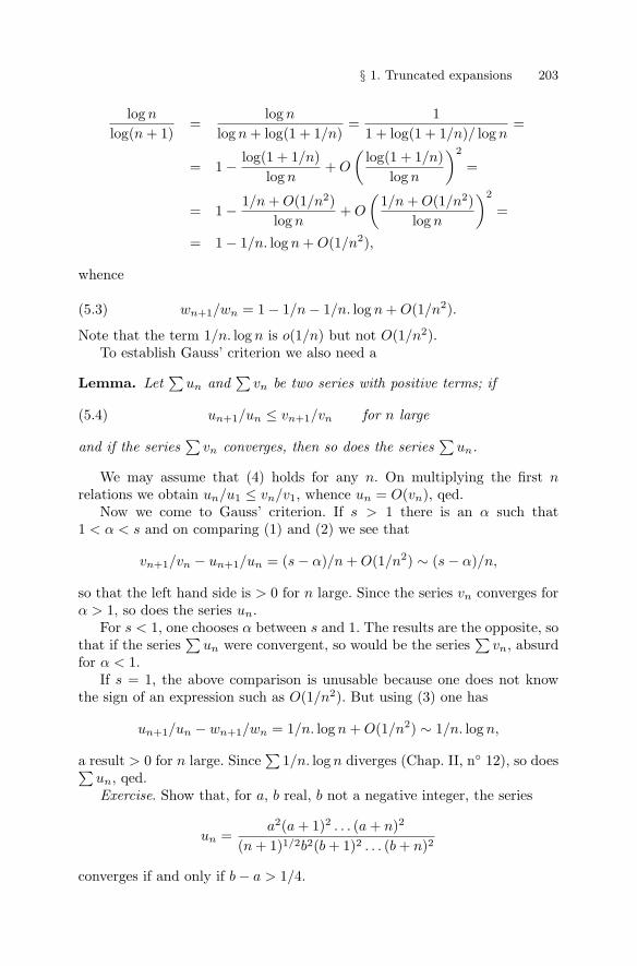
§ 1. Truncated expansions 203
log n
log(n + 1)=
log n
log n + log(1 + 1/n)=
11 + log(1 + 1/n)/ log n
=
= 1 − log(1 + 1/n)log n
+ O
(log(1 + 1/n)
log n
)2
=
= 1 − 1/n + O(1/n2)log n
+ O
(1/n + O(1/n2)
log n
)2
=
= 1 − 1/n. log n + O(1/n2),
whence
wn+1/wn = 1 − 1/n − 1/n. log n + O(1/n2).(5.3)
Note that the term 1/n. log n is o(1/n) but not O(1/n2).To establish Gauss’ criterion we also need a
Lemma. Let∑
un and∑
vn be two series with positive terms; if
un+1/un ≤ vn+1/vn for n large(5.4)
and if the series∑
vn converges, then so does the series∑
un.
We may assume that (4) holds for any n. On multiplying the first nrelations we obtain un/u1 ≤ vn/v1, whence un = O(vn), qed.
Now we come to Gauss’ criterion. If s > 1 there is an α such that1 < α < s and on comparing (1) and (2) we see that
vn+1/vn − un+1/un = (s − α)/n + O(1/n2) ∼ (s − α)/n,
so that the left hand side is > 0 for n large. Since the series vn converges forα > 1, so does the series un.
For s < 1, one chooses α between s and 1. The results are the opposite, sothat if the series
∑un were convergent, so would be the series
∑vn, absurd
for α < 1.If s = 1, the above comparison is unusable because one does not know
the sign of an expression such as O(1/n2). But using (3) one has
un+1/un − wn+1/wn = 1/n. log n + O(1/n2) ∼ 1/n. log n,
a result > 0 for n large. Since∑
1/n. log n diverges (Chap. II, n◦ 12), so does∑un, qed.Exercise. Show that, for a, b real, b not a negative integer, the series
un =a2(a + 1)2 . . . (a + n)2
(n + 1)1/2b2(b + 1)2 . . . (b + n)2
converges if and only if b − a > 1/4.
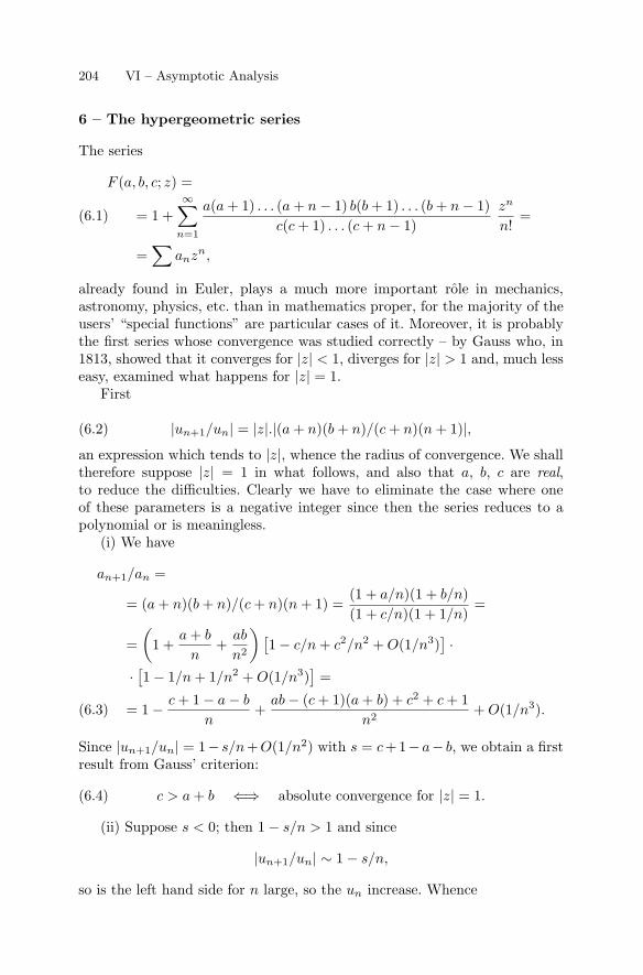
204 VI – Asymptotic Analysis
6 – The hypergeometric series
The series
F (a, b, c; z) =
= 1 +∞∑
n=1
a(a + 1) . . . (a + n − 1) b(b + 1) . . . (b + n − 1)c(c + 1) . . . (c + n − 1)
zn
n!=(6.1)
=∑
anzn,
already found in Euler, plays a much more important role in mechanics,astronomy, physics, etc. than in mathematics proper, for the majority of theusers’ “special functions” are particular cases of it. Moreover, it is probablythe first series whose convergence was studied correctly – by Gauss who, in1813, showed that it converges for |z| < 1, diverges for |z| > 1 and, much lesseasy, examined what happens for |z| = 1.
First
|un+1/un| = |z|.|(a + n)(b + n)/(c + n)(n + 1)|,(6.2)
an expression which tends to |z|, whence the radius of convergence. We shalltherefore suppose |z| = 1 in what follows, and also that a, b, c are real,to reduce the difficulties. Clearly we have to eliminate the case where oneof these parameters is a negative integer since then the series reduces to apolynomial or is meaningless.
(i) We have
an+1/an =
= (a + n)(b + n)/(c + n)(n + 1) =(1 + a/n)(1 + b/n)(1 + c/n)(1 + 1/n)
=
=(
1 +a + b
n+
ab
n2
)[1 − c/n + c2/n2 + O(1/n3)
] ·· [1 − 1/n + 1/n2 + O(1/n3)
]=
= 1 − c + 1 − a − b
n+
ab − (c + 1)(a + b) + c2 + c + 1n2
+ O(1/n3).(6.3)
Since |un+1/un| = 1− s/n+O(1/n2) with s = c+1−a− b, we obtain a firstresult from Gauss’ criterion:
c > a + b ⇐⇒ absolute convergence for |z| = 1.(6.4)
(ii) Suppose s < 0; then 1 − s/n > 1 and since
|un+1/un| ∼ 1 − s/n,
so is the left hand side for n large, so the un increase. Whence
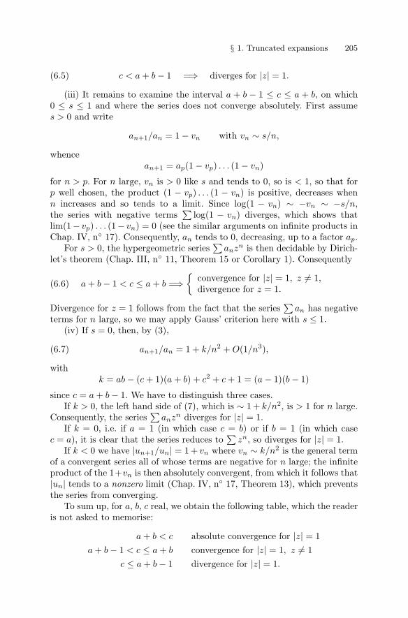
§ 1. Truncated expansions 205
c < a + b − 1 =⇒ diverges for |z| = 1.(6.5)
(iii) It remains to examine the interval a + b − 1 ≤ c ≤ a + b, on which0 ≤ s ≤ 1 and where the series does not converge absolutely. First assumes > 0 and write
an+1/an = 1 − vn with vn ∼ s/n,
whencean+1 = ap(1 − vp) . . . (1 − vn)
for n > p. For n large, vn is > 0 like s and tends to 0, so is < 1, so that forp well chosen, the product (1 − vp) . . . (1 − vn) is positive, decreases whenn increases and so tends to a limit. Since log(1 − vn) ∼ −vn ∼ −s/n,the series with negative terms
∑log(1 − vn) diverges, which shows that
lim(1− vp) . . . (1− vn) = 0 (see the similar arguments on infinite products inChap. IV, n◦ 17). Consequently, an tends to 0, decreasing, up to a factor ap.
For s > 0, the hypergeometric series∑
anzn is then decidable by Dirich-let’s theorem (Chap. III, n◦ 11, Theorem 15 or Corollary 1). Consequently
a + b − 1 < c ≤ a + b =⇒{
convergence for |z| = 1, z �= 1,divergence for z = 1.(6.6)
Divergence for z = 1 follows from the fact that the series∑
an has negativeterms for n large, so we may apply Gauss’ criterion here with s ≤ 1.
(iv) If s = 0, then, by (3),
an+1/an = 1 + k/n2 + O(1/n3),(6.7)
withk = ab − (c + 1)(a + b) + c2 + c + 1 = (a − 1)(b − 1)
since c = a + b − 1. We have to distinguish three cases.If k > 0, the left hand side of (7), which is ∼ 1 + k/n2, is > 1 for n large.
Consequently, the series∑
anzn diverges for |z| = 1.If k = 0, i.e. if a = 1 (in which case c = b) or if b = 1 (in which case
c = a), it is clear that the series reduces to∑
zn, so diverges for |z| = 1.If k < 0 we have |un+1/un| = 1+ vn where vn ∼ k/n2 is the general term
of a convergent series all of whose terms are negative for n large; the infiniteproduct of the 1+vn is then absolutely convergent, from which it follows that|un| tends to a nonzero limit (Chap. IV, n◦ 17, Theorem 13), which preventsthe series from converging.
To sum up, for a, b, c real, we obtain the following table, which the readeris not asked to memorise:
a + b < c absolute convergence for |z| = 1a + b − 1 < c ≤ a + b convergence for |z| = 1, z �= 1
c ≤ a + b − 1 divergence for |z| = 1.
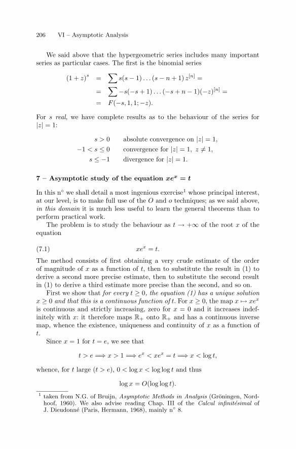
206 VI – Asymptotic Analysis
We said above that the hypergeometric series includes many importantseries as particular cases. The first is the binomial series
(1 + z)s =∑
s(s − 1) . . . (s − n + 1) z[n] =
=∑
−s(−s + 1) . . . (−s + n − 1)(−z)[n] =
= F (−s, 1, 1;−z).
For s real, we have complete results as to the behaviour of the series for|z| = 1:
s > 0 absolute convergence on |z| = 1,−1 < s ≤ 0 convergence for |z| = 1, z �= 1,
s ≤ −1 divergence for |z| = 1.
7 – Asymptotic study of the equation xex = t
In this n◦ we shall detail a most ingenious exercise1 whose principal interest,at our level, is to make full use of the O and o techniques; as we said above,in this domain it is much less useful to learn the general theorems than toperform practical work.
The problem is to study the behaviour as t → +∞ of the root x of theequation
xex = t.(7.1)
The method consists of first obtaining a very crude estimate of the orderof magnitude of x as a function of t, then to substitute the result in (1) toderive a second more precise estimate, then to substitute the second resultin (1) to derive a third estimate more precise than the second, and so on.
First we show that for every t ≥ 0, the equation (1) has a unique solutionx ≥ 0 and that this is a continuous function of t. For x ≥ 0, the map x → xex
is continuous and strictly increasing, zero for x = 0 and it increases indef-initely with x: it therefore maps R+ onto R+ and has a continuous inversemap, whence the existence, uniqueness and continuity of x as a function oft.
Since x = 1 for t = e, we see that
t > e =⇒ x > 1 =⇒ ex < xex = t =⇒ x < log t,
whence, for t large (t > e), 0 < log x < log log t and thus
log x = O(log log t).1 taken from N.G. of Bruijn, Asymptotic Methods in Analysis (Groningen, Nord-
hoof, 1960). We also advise reading Chap. III of the Calcul infinitesimal ofJ. Dieudonne (Paris, Hermann, 1968), mainly n◦ 8.
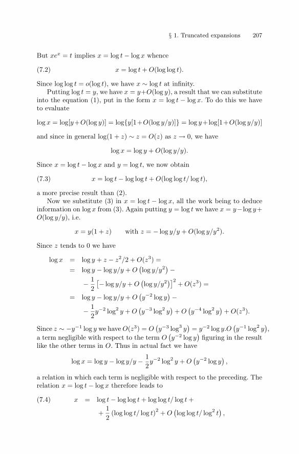
§ 1. Truncated expansions 207
But xex = t implies x = log t − log x whence
x = log t + O(log log t).(7.2)
Since log log t = o(log t), we have x ∼ log t at infinity.Putting log t = y, we have x = y+O(log y), a result that we can substitute
into the equation (1), put in the form x = log t − log x. To do this we haveto evaluate
log x = log[y+O(log y)] = log{y[1+O(log y/y)]} = log y+log[1+O(log y/y)]
and since in general log(1 + z) ∼ z = O(z) as z → 0, we have
log x = log y + O(log y/y).
Since x = log t − log x and y = log t, we now obtain
x = log t − log log t + O(log log t/ log t),(7.3)
a more precise result than (2).Now we substitute (3) in x = log t − log x, all the work being to deduce
information on log x from (3). Again putting y = log t we have x = y− log y+O(log y/y), i.e.
x = y(1 + z) with z = − log y/y + O(log y/y2).
Since z tends to 0 we have
log x = log y + z − z2/2 + O(z3) == log y − log y/y + O
(log y/y2
)−− 1
2[− log y/y + O
(log y/y2
)]2+ O(z3) =
= log y − log y/y + O(y−2 log y
)−− 1
2y−2 log2 y + O
(y−3 log2 y
)+ O(y−4 log2 y
)+ O(z3).
Since z ∼ −y−1 log y we have O(z3) = O(y−3 log3 y
)= y−2 log y.O
(y−1 log2 y
),
a term negligible with respect to the term O(y−2 log y
)figuring in the result
like the other terms in O. Thus in actual fact we have
log x = log y − log y/y − 12y−2 log2 y + O
(y−2 log y
),
a relation in which each term is negligible with respect to the preceding. Therelation x = log t − log x therefore leads to
x = log t − log log t + log log t/ log t +(7.4)
+12
(log log t/ log t)2 + O(log log t/ log2 t
),
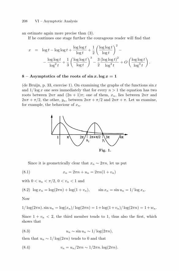
208 VI – Asymptotic Analysis
an estimate again more precise than (3).If he continues one stage further the courageous reader will find that
x = log t − log log t +log log t
log t+
12
(log log t
log t
)2
−
− log log t
log2 t+
13
(log log t
log t
)3
− 32
(log log t)2
log3 t+ O
(log log t
log3 t
).
8 – Asymptotics of the roots of sin x. log x = 1
(de Bruijn, p. 33, exercise 1). On examining the graphs of the functions sinxand 1/ log x one sees immediately that for every n > 1 the equation has tworoots between 2nπ and (2n + 1)π; one of them, xn, lies between 2nπ and2nπ + π/2, the other, yn, between 2nπ + π/2 and 2nπ + π. Let us examine,for example, the behaviour of xn.
Fig. 1.
Since it is geometrically clear that xn ∼ 2πn, let us put
xn = 2πn + un = 2πn(1 + vn)(8.1)
with 0 < un < π/2, 0 < vn < 1 and
log xn = log(2πn) + log(1 + vn), sin xn = sin un = 1/ log xn.(8.2)
Now
1/ log(2πn). sin un = log(xn)/ log(2πn) = 1+log(1+vn)/ log(2πn) = 1+wn.
Since 1 + vn < 2, the third member tends to 1, thus also the first, whichshows that
un ∼ sin un ∼ 1/ log(2πn),(8.3)
then that un ∼ 1/ log(2πn) tends to 0 and that
vn = un/2πn ∼ 1/2πn. log(2πn).(8.4)
§ 1. Truncated expansions 209
Hence
wn = log(1 + vn)/ log(2πn) =[vn + O
(v2
n
)]/ log(2πn).
Since wn tends to 0 we have
log(2πn). sin un == 1/(1 + wn) = 1 − wn + O
(w2
n
)= 1 − vn/ log(2πn) + O
(v2
n
)/ log(2πn) + O
(v2
n
)/ log2(2πn) =
= 1 − vn/ log(2πn) + O(v2
n
)/ log(2πn),
whence
sin un = 1/ log(2πn) − vn/ log2(2πn) + O(v2
n
)/ log2(2πn).(8.5)
But sin un = un + O(u3
n
)= un + O
(1/ log3(2πn)
)by (3), whence
un = 1/ log(2πn) − vn/ log2(2πn) ++ O(v2
n
)/ log2(2πn) + O
(1/ log3(2πn)
)=
= 1/ log(2πn) + O(1/n log3(2πn)
)+
+ O(1/n2 log4(2πn)
)+ O(1/ log3(2πn)
).
On the right hand side the second and the third terms are negligible withrespect to last, which therefore dominates. At the point where we are nowwe cannot say anything more precise than
un = 1/ log(2πn) + O(1/ log3(2πn)
),(8.6)
which nevertheless improves on (3).To get further we write that sinun = un −u3
n/6+O(u5
n
). Using (6) gives
sin un = un − [1/ log(2πn) + O(1/ log3(2πn
)]3/6 + O
(1/ log5(2πn)
)=
= un − [1/ log3(2πn) + O(1/ log5(2πn)
)]/6 + O
(1/ log5(2πn)
),
whence, by (5),
un = 1/ log(2πn) − vn/ log2(2πn) + O(v2
n
)/ log2(2πn) +
+ 1/6 log3(2πn) + O(1/ log5(2πn)
)+ O(1/ log5(2πn)
);
since vn = O(1/n. log(2πn)
)by (4), the terms containing vn are negligible
with respect to O(1/ log5(2πn)
)and there remains
un = 1/ log(2πn) + 1/6 log3(2πn) + O(1/ log5(2πn)
),(8.7)
which improves (6). Here, as in the preceding n◦, the reader can continue thecalculations and/or examine the behaviour of the other series of roots yn.
210 VI – Asymptotic Analysis
9 – Kepler’s equation
We saw in Chap. II, at the end of n◦ 16, that Kepler’s equation u−e. sin u = ωthas one and only one root u provided that the eccentricity e of the ellipticalmotion is < 1. To simplify the notation a little, and to avoid confusing e with2, 71828 . . ., let us write it as
u = ϕ + ε sin u.(9.1)
Laplace (see the 130-page notice by Gillispie in the supplement to DSB),the author of a treatise on celestial mechanics much more advanced thanNewton’s Principia, proved (?) that u is the sum of a power series in ε whosecoefficients, depending on ϕ, are determined by an extraordinarily simpleformula:
u = ϕ + ε(sin ϕ)/1! + ε2(sin2 ϕ)′/2! + ε3(sin3 ϕ)′′/3! + . . . .(9.2)
One can make (2) plausible by putting u = ϕ + v, so that v = ε sin utends to 0 with ε, and seeking an asymptotic evaluation of v; this does notreplace a power series, but one works with the tools at one’s disposal.
Clearly v = O(ε) and indeed
v = ε(sin ϕ. cos v + cos ϕ. sin v) == ε sin ϕ
(1 + O(ε2)
)+ ε cos ϕ.O(ε) = ε sin ϕ + O(ε2),
whence
u = ϕ + ε sin ϕ + O(ε2) = ϕ + ε sin ϕ + ε2w with w = O(1).
Then by (1)
ε sin ϕ + ε2w = ε sin ϕ(ϕ + ε sin ϕ + ε2w
)=
= ε sin ϕ. cos(ε sin ϕ + ε2w
)+ ε cos ϕ. sin
(ε sin ϕ + ε2w
)=
= ε sin ϕ.[1 − (ε sin ϕ + ε2w
)2/2 + O(ε4)
]+
+ ε cos ϕ.[ε sin ϕ + ε2w + O(ε3)
],
whence
ε2w = ε2 sin ϕ cos ϕ + ε3(w cos ϕ − sin3 ϕ/2
)+ O(ε4)
i.e.w = sin ϕ cos ϕ + ε
(w cos ϕ − sin3 ϕ/2
)+ O(ε2).
Since w = O(1), i.e. is bounded, one infers immediately that w = sin ϕ cos ϕ+O(ε), whence, substituting in the right hand side of the preceding relation,
w = sin ϕ cos ϕ + ε(sin ϕ. cos2 ϕ − sin3 ϕ/2
)+ O(ε2).
§ 1. Truncated expansions 211
Thus
u = ϕ + ε sin ϕ + ε2 sin ϕ cos ϕ + ε3(sin ϕ. cos2 ϕ − sin3 ϕ/2
)+ O(ε4),
which yields the first terms of formula (2). The calculation becomes moreand more painful as one pushes further and further.
The result was then extended by Lagrange to much more general equa-tions, namely, in his notation,
z = x + yf(z).(9.3)
Since, for these Gentlemen, all functions arising in Nature, or even in math-ematics, are analytic outside isolated points – as it happens, they were rightto believe so if f is, but then to prove this . . . –, Lagrange set himself tocalculate the expansion of z =
∑anyn as a power series, where the coeffi-
cients an of course depend on x. The direct way would be, for x given, todifferentiate (3) indefinitely with respect to y, and to deduce the relations
z′ = f(z) + yf ′(z)z′, z′′ = 2f ′(z)z′ + y[f ′′(z)z′2 + f ′(z)z′′
],
z′′′ = 2f ′′(z)z′2 + 2f ′(z)z′′ + f ′′(z)z′2 + f ′(z)z′′ ++ y[f ′′′(z)z′3 + 2f ′′(z)z′z′′ + f ′′(z)z′z′′ + f ′(z)z′′′
],
etc. and to find successively their values for y = 0:
z(0) = x, z′(0) = f(x), z′′(0) = 2f ′(x)f(x) =[f(x)2]′
,
z′′′(0) = 3f ′′(x)f(x)2 + 6f ′(x)2f(x) =[f(x)3]′′
,
etc. This is, in an other form, what we have done above for Kepler’s equation.The first results suggest the formula
z = x +∑
yn [f(x)n](n−1)/n!(9.4)
using Maclaurin. But one falls rapidly, as above, into impossible calculations.Lagrange’s method of establishing (4), at least formally, is considerably moreingenious.
His idea was to consider z as a function of y and of x and to differentiate(3) with respect to each of these two variables in order to calculate thecoefficients Dn
2 z(x, 0) of the Maclaurin series of z with respect to y.To start with, thanks to the Chain Rule (Chap. III, n◦ 21), one finds
D1z = 1 + yf ′(z)D1z, D2z = f(z) + yf ′(z)D2z,(9.5)
whence (D1z − 1)D2z = [D2z − f(z)] D1z, and consequently
D2z = f(z)D1z.(9.6)
212 VI – Asymptotic Analysis
For y = 0, (5) gives
D1z(x, 0) = 1, D2z(x, 0) = f(x)(9.7)
since then z = x. Differentiating (6) with respect to y,
D22z = f ′(z)D2zD1z + f(z)D2D1z = f ′(z)D2zD1z + f(z)D1D2z =
= D1 [D2z.f(z)] = D1
[D1z.f(z)2
]by (6) and D1D2 = D2D1 (Chap. III, n◦ 23). Whence D2
2z(x, 0) =[f(x)2]′
since, for y = 0, we have D2z.f(z) = f(x)2 by (7). Suppose we have provedthat
Dn2 z = Dn−1
1 [D1z.f(z)n](9.8)
for any x and y, and differentiate. Using (6) again, and D1D2 = D2D1, weget
Dn+12 z = Dn−1
1 D2 [D1z.f(z)n] == Dn−1
1
[D2D1z.f(z)n + D1z.nf(z)n−1f ′(z)D2z
]=
= Dn−11
[D1D2z.f(z)n + D2z.nf(z)n−1f ′(z)D1z
]=
= Dn1 [D2z.f(z)n] = Dn
1
[D1z.f(z)n+1
],
which is (8) for n + 1.The relation (8) is therefore valid for any n and yields the formula
Dn2 z(x, 0) = [f(x)n](n−1)
which justifies (4), at least formally.In fact, Lagrange went even further; instead of just expanding z he ex-
panded an “arbitrary” function of z, say u = ϕ(z). Since D1u = ϕ′(z)D1zand D2u = ϕ′(z)D2z, the relation (6) becomes
D2u = f(z)D1u,
which allows one to calculate as we have just done, this time with
Dn2 u(x, 0) = [ϕ′(x)f(x)n](n−1)(9.9)
and “thus”ϕ(z) = ϕ(x) +
∑yn [ϕ′(x)f(x)n](n−1)
/n!.
The proof consists of establishing the relation
Dn2 u = Dn−1
1 [D1u.f(z)n] ,
which replaces (8), by induction as above; for y = 0 we have D1u =ϕ′(z)D1z = ϕ′(x), whence (9).
§ 1. Truncated expansions 213
10 – Asymptotics of the Bessel functions
Consider the differential equation
x′′ + (1 − c/t2)x = 0,(10.1)
where x is an unknown function of the real variable t �= 0 and c is a nonzeroconstant. We set ourselves to study the asymptotic behaviour of its solutionsfor t large. We shall divide this relatively difficult but highly instructive ex-ercise into several parts.
Passage to an integral equation
Since (1) can be written
x′′ + x = cx/t2,(10.1’)
one may assume that at infinity its solutions resemble those of the muchsimpler equation y′′ +y = 0, which has as its solutions at least (and, we shallsee, at most) the functions
y(t) = aeit + be−it, whence y′(t) = iaeit − ibe−it,
where a and b are arbitrary constants. In the general case one puts
x(t) = a(t)eit + b(t)e−it, x′(t) = ia(t)eit − ib(t)e−it(10.2)
where a(t) and b(t) are now functions that one may easily calculate from xand x′, by multiplying the relations (2) by eit or e−it. This is the methodof variation of constants (Johann Bernoulli, end of the XVIIth century, forequations of the first order, Lagrange in the general case) which applies toall differential equations in which the unknown function and its derivativesoccur linearly, but which one applies here in a nonclassical way since one ismaking believe that the function cx(t)t−2 occurring on the right hand sideof (1’) is known [if it were the method would provide all the solutions of (1’)in terms of integrals involving the right hand side].
The second relation (2), which seems to contradict the Chain Rule grossly,is in fact equivalent to
a′(t)eit + b′(t)e−it = 0.(10.3)
It then follows that
x′′ = −aeit − be−it + ia′eit − ib′e−it = −x + ia′eit − ib′e−it
by the relations (2). Equation (1) can therefore be written as
ia′(t)eit − ib′(t)e−it = cx(t)/t2.(10.4)
214 VI – Asymptotic Analysis
One deduces from (3) and (4) that
2ia′(t) = ct−2x(t)e−it, 2ib′(t) = −ct−2x(t)eit,(10.5)
whence, using the FT,
2ia(t) − 2ia(t0) = c
∫ t
t0
x(u)e−iuu−2du,
2ib(t) − 2ib(t0) = −c
∫ t
t0
x(u)eiuu−2du.
We must assume t0 �= 0 and t of the same sign as t0 because of the factoru−2, not integrable on a neighbourhood of 0. We shall assume them > 0 inall that follows, the opposite case being treated similarly. Substituting in thefirst relation (2), one finds
x(t) = p0(t) + c
∫ t
t0
x(u) sin(t − u)u−2du(10.6)
with p0(t) = a0eit + b0e
−it, where a0 = a(t0), b0 = b(t0). Instead of, like (1),involving the function x and its derivatives, (6) involves x and an integralfeaturing the function x itself; this is an integral equation. It does not evenassume x to be differentiable: the continuity of x is enough for (6) to makesense. It is (6) which will allow us to examine the behaviour of x at infinity.
One may conversely verify that every continuous solution of (6) is in factC∞ and satisfies (1). The theorem on differentiation under the
∫sign with
variable limits (Chap. V, n◦ 12, Theorem 13) in fact shows that the righthand side is differentiable and that
x′(t) = p′0(t) + c
∫ t
t0
x(u) cos(t − u)u−2du,(10.7)
since the function integrated in (6) is zero for u = t. This relation in its turnshows that x′ is differentiable and that
x′′(t) = p′′0(t) − c
∫ t
t0
x(u) sin(t − u)u−2du + cx(t)t−2(10.8)
since x(u) cos(t− u)u−2 = x(t)t−2 for u = t. Since p0 + p′′0 = 0, one finds (1)again, on adding the result to (6). The fact that x is C∞ is then obvious,either because the function integrated in (6) has continuous derivatives ofarbitrary order with respect to t, or because the differential equation showsthat if x is Cp, then it is automatically Cp+2 away from the origin.
First bound for the solutions
§ 1. Truncated expansions 215
Let us agree provisionally that there is a solution of (6) defined for t > 0and then show it is bounded at infinity. Indeed, let M(t) be the upper boundof |x(u)| on the interval [t0, t] and M0 that of |p0(u)| in R, clearly finite.(6) shows that, for t0 ≤ t′ ≤ t,
|x(t′)| ≤ M0 + |c|M(t)∫ t′
t0
u−2du ≤ M0 + |c|M(t)/t0,
whence, passing to the sup,
M(t) ≤ M0 + |c|M(t)/t0.(10.9)
If we have chosen t0 large enough that |c|/t0 ≤ 12 we may deduce that M(t) ≤
2M0, qed.Now let us show that there exist constants a1, b1 such that
x(t) = a1eit + b1e
−it + O(1/t) = p1(t) + O(1/t).(10.10)
Since x(t) is indeed bounded, the integral in (6), taken from t0 to +∞, isabsolutely convergent like that of the function 1/u2. Thus
x(t) = p0(t) + c
∫ +∞
t0
x(u) sin(t − u)u−2du −(10.11)
− c
∫ +∞
t
x(u) sin(t − u)u−2du.
Expressing sin(t − u) in terms of complex exponentials, we see that the firstintegral is, like p0(t), a linear combination of eit and e−it with coefficientsindependent of t, whence
x(t) = p1(t) − c
∫ +∞
t
x(u) sin(t − u)u−2du(10.12)
where p1(t) is a linear combination of eit and e−it with constant coefficients.Since the function x(u) sin(t − u) is bounded for u ≥ t0 > 0, the integral is,up to a constant factor, majorised by that of u−2, i.e. by 1/t, qed.
The relation (12) allows us to complete the existence theorem for solutions– we shall prove it below – with a uniqueness theorem: there exists only onesolution of (12) for p1 given. Since p1 depends on two arbitrary constants,this means that the set of solutions is a vector space of dimension 2 over C.
On subtraction we reduce to proving that, if p1 is zero, then so likewiseis x. But denote now by M(t) the upper bound of |x(u)| for u ≥ t. For t′ ≥ twe clearly have
|x(t′)| ≤ |c|M(t)/t
since the integral of u−2 between t′ and +∞, equal to 1/t′, is ≤ 1/t. Whence,on passing to the sup, M(t) ≤ |c|M(t)/t. Substituting this result in theintegral equation, we now find
216 VI – Asymptotic Analysis
|x(t′)| ≤ |c|2M(t)∫ +∞
t′u−3du,
whence M(t) ≤ |c|2M(t)/2t2. Substituting again in the equation, we willfind M(t) ≤ |c|3M(t)/3!t3, etc. In short, M(t) ≤ M(t)|c/t|n/n! for any n.Since, for t �= 0 given, the right hand side tends to 0 when n → +∞, we findM(t) = 0 for any t > 0, whence x(t) = 0, qed.
Existence of solutions
To go further than (10) in studying x(t) at infinity, one might, as always,iterate the calculation, i.e. substitute (10) in (12) and so on indefinitely.We are going to adopt a slightly different method which will at the sametime show the existence of the solutions; this is the method of successiveapproximations, which consists of extending the method of constructing theroots of an equation x = f(x) expounded in Chap. II, n◦ 16, Theorem 12 andin Chap. III, n◦ 24 (implicit functions) to integral equations; it can be used toshow the existence, at least locally, of the solutions of almost all reasonabledifferential or integral equations. Since all the integrals which now appearare extended over [t, +∞], we shall adopt the simplified notation∫
=∫ +∞
t
up to the end of this n◦, clearly not confusing this with an indefinite integrala la Leibniz. In this notation∫
u−n−1du = t−n/n
for n ≥ 1 by the FT.The method of successive approximations consists of starting from the
function p1(t) in (12), to which x(t) is equal up to the addition of a O(1/t)term, constructing a sequence of functions xn(t) on t > 0 by putting x1 = p1
and
xn+1(t) = p1(t) − c
∫xn(u) sin(t − u)u−2du,(10.13)
and showing that the xn converge to a solution of (6).For n = 1
|x2(t) − x1(t)| ≤ M |c|∫
u−2du = M |c/t|
where M = ‖p1‖R< +∞. It follows that
|x3(t) − x2(t)| = |c|.∣∣∣∣∫
[x2(u) − x1(u)] sin(t − u)u−2du
∣∣∣∣ ≤≤ M |c|2
∫u−3du = M |c/t|2/2!.
§ 1. Truncated expansions 217
If one has proved that
|xn(t) − xn−1(t)| ≤ M |c/t|n−1/(n − 1)!(10.14)
one finds
|xn+1(t) − xn(t)| = |c|.∣∣∣∣∫
[xn(u) − xn−1(u)] sin(t − u)u−2du
∣∣∣∣ ≤≤ M |c|n/(n − 1)!
∫u−n−1du = M |c/t|n/n!,
which shows in passing that
xn+1(t) = xn(t) + O(t−n)(10.15)
at infinity. Since the series∑
[xn+1(t) − xn(t)] is, by (14), dominated by theseries exp(M |c|/t), it converges normally on every interval t ≥ t0 > 0, sothat xn(t) converges to a limit x(t) for every t > 0, and does so uniformlyon every interval [t0,+∞[. One may then pass to the limit under the
∫sign
in (13) because of the presence of the integrable2 factor u−2. It is then clearthat x(t) satisfies (6).
Further, by (14),
|x(t) − xn(t)| ≤∑p≥0
|xn+p+1(t) − xn+p(t)| ≤
≤ M∑p≥0
|c/t|n+p/(n + p)! ≤ M
∑p≥0
|c/t|n+p/n!p! =
= M. exp(|c/t|)|c/t|n/n!,
a result which implies
x(t) = xn(t) + O(t−n)(10.16)
at infinity since the factor exp(|c/t|) tends to 1.Exercise. Let I be a compact interval, p a continuous function on I and
K(t, u) a continuous function on I × I. Put
M = supt∈I
∫|K(t, u)|du.
Show that, if M < 1, the integral equation2 Let I be an arbitrary interval, µ(x) an absolutely integrable function on I,
and (fn) a sequence of bounded functions which converges uniformly on I toa limit f , clearly bounded. The functions fnµ and fµ, majorised up to con-stant factors by µ, are then integrable and one has
∣∣∫ [fn(u) − f(u)] µ(u)du∣∣ ≤
‖fn − f‖ .∫ |µ(u)|du, whence lim
∫fn(u)µ(u)du =
∫f(u)µ(u)du. Cf. Chap. V,
n◦ 31, Example 1.
218 VI – Asymptotic Analysis
x(t) = p(t) +∫
K(t, u)x(u)du
has one and only one solution (the integrals are over I). Analogy with a sys-tem of linear equations?
Asymptotics of the solutions: general form
It is clear that in order to obtain asymptotic evaluations of x(t) one shouldseek them for the xn(t). To simplify the calculations we shall assume thatwe are in the case where the “trigonometric binomial” p1(t) in (10) reducesto eit; the case where it is equal to e−it is treated in the same way (the twosolutions are even complex conjugates if c ∈ R), and in the general case it isclear that x is a linear combination of the functions corresponding to thesetwo particular cases.
Since x1(t) = eit, the relation (13) shows that
2ix2(t) = 2ieit − 2ic
∫eiu sin(t − u)u−2du =(10.17)
= 2ieit − c
∫ (eit − e2iu−it
)u−2du =
= 2ieit − ceit/t + ce−it
∫e2iuu−2du.
Here we meet, and we will meet again, an integral of the form∫
e2iuu−pduextended over [t,+∞[. By repeatedly integrating by parts it is easy to find atruncated expansion of arbitrarily high order when t tends to infinity. Gen-erally, if Re(α) ≤ 0 to ensure the convergence of the integrals, one has, usingexceptionally the
∫sign a la Leibniz,∫
eαuu−pdu = eαu/αup +p
α
∫eαuu−p−1du =
= eαu/αup + peαu/α2up+1 +p(p + 1)
α2
∫eαuu−p−2du
etc3. When one integrates from t to +∞, the integrated-out parts, zero atinfinity, yield the product of eαt/tp by a polynomial in 1/t; the integral ofeαuu−N−2, majorised by that of u−N−2, is O
(t−N−1). One deduces from this
that, for any N > p, there is a relation3 Note that instead of trying to pass from an integral in u−p to an integral in u−p+1
as was done in Chap. V, n◦ 15, Example 2 in the illusory hope of calculatinga primitive explicitly, here one passes from an integral in u−p to integrals inu−p−1, u−p−2, etc. whose order of magnitude one may evaluate, even if unableto calculate them explicitly.
§ 1. Truncated expansions 219
e−it
∫ +∞
t
e2iuu−pdu = −eit(?/tp+?/tp+1 + . . . +?/tN
)+(10.18)
+ O(t−N−1)
with coefficients ? which depend on p, but not on N ; the reader may calculatethem: we don’t need them now. Returning to (17), the case where p = 2, wefinally find
2ix2(t) = 2ieit + eit(?/t+?/t2 + . . . +?/tN
)+ O(t−N−1)
(10.19)
for any N .It is the same for xn(t) for any n. One shows this by induction using (13):
2ixn+1(t) =
= 2ieit − 2ic
∫xn(u) sin(t − u)u−2du =
= 2ieit − c
∫eiu[?−?/u − . . .−?/uN + O
(u−N−1
)]2i sin(t − u)u−2du =
= 2ieit + c∑
0≤p≤N
?∫ (
eit − e2iu−it)u−p−2du +
∫O(u−N−3
)du.
The integrals∫
eitu−p−2du yield the product of eit by a polynomial in1/t without constant term. The integrals
∫e2iu−itu−p−2du likewise by (18)
have truncated expansions of arbitrarily high order. Finally, the integral∫O(u−N−3
)du is O
(t−N−2). So for every n and every N there is a relation
of the form
xn(t) = eit(1+?/t+?/t2 + . . . +?/tN
)+ O(t−N−1).(10.20)
In view of (16) one obtains an expansion
x(t) = eit(1 + a1/t + a2/t2 + . . . + aN/tN
)+ O(t−N−1)
(10.21)
for x(t), whose coefficients do not depend on N ; for if one has this for e−itx(t)or for every other function with truncated expansions of order 12 and 15, thesecond, with its terms of degree > 12 removed, yields a truncated expansionof order 12; now a given function can have only one truncated expansion ofgiven order, as we saw in n◦ 3; the two expansions must therefore have thesame terms of degree ≤ 12.
One sometimes expresses this fact by writing (21) in the form of an as-ymptotic series
e−itx(t) ≈∞∑
n=0
an/tn;(10.22)
this way of writing by no means states that the series on the right hand siderepresents the function considered: in almost every case of this kind, including
220 VI – Asymptotic Analysis
the one which now occupies us, as we shall see when all will be calculated, theseries is divergent. The form (22) is, by definition, equivalent to the fact thatthe relation (21) is valid for any N . In other words, the difference betweenthe left hand side of (22) and the N -th partial sum of the second member,instead of tending to 0 for t given when N increases, tends to 0 for N givenwhen t increases, and as rapidly as the first term neglected; a nuance not tobe forgot . . .
This is for example what happens on a neighbourhood of t = 0 when onewrites the Maclaurin formula for a function x(t) which is not analytic but isof class C∞. For any N , one has
x(t) = x(0) + x′(0)t + . . . + x(N)(0)tN/N ! + O(tN+1),
in other wordsx(t) ≈
∑x(n)(0)tn/n!,
but the series has no reason to represent the function if it converges – thecase of exp(−1/t2) – and even less if it diverges, which is the general casesince the derivatives at the origin can be chosen arbitrarily (Chap. V, n◦ 29).
Term-by-term differentiation of asymptotic expansions
The problem now arises of calculating the coefficients an in the expansion(22) explicitly, preferably without drowning oneself in calculation. In doingthis in a more explicit way than we have done above we could find the recur-rence relations allowing us to calculate the an. A more elegant4 and aboveall more instructive, method, consists of showing that on differentiating (22)term-by-term, one obtains the analogous asymptotic expansions for x′ andx′′; on substituting into the differential equation (1) one will find the neededrecurrence relations immediately.
It is not at all obvious, and it is generally false, that one can deducean asymptotic series for the derivative from the asymptotic series of a givenfunction by differentiating term-by-term. The derivative of a function O(tr)at infinity (r ∈ R) has no reason to be O
(tr−1): the function x(t) = sin(t2)/t
is O(1/t) at infinity, but its derivative x′(t) = 2 cos(t2) − sin(t2)/t2 is O(1)and not O(1/t2) at infinity. This is the problem we have already met inconnection with differentiating term-by-term the sum of a series of differen-tiable functions: one may, thanks to FT, majorise a function starting from amajoration of its derivative, but the inverse operation is impossible.4 One of the Goncourt brothers, famous literary critics of the XIXth century, relates
in his Journal that during the reception of a new immortal, X, into the Academiefrancaise, the academician Y charged with delivering the eulogy on X had theregrettable idea of describing the oratorical style of X as elegant. The latter,furious, stood up and replied: Elegant yourself, Sir! (I quote from memory).
§ 1. Truncated expansions 221
The reality is that here, as in the case of a convergent series or sequence,it is the existence of an asymptotic series for the derivative which enablesus to obtain one for the function itself. For assume that the derivative of afunction f(t) has an expansion
f ′(t) = a0 + a1/t + . . . + aN+1/tN+1 + O(1/tN+2
)(10.23)
at infinity. One cannot integrate it from t to +∞ because of the first twoterms, but one reduces to the case where they are zero on replacing f(t) byg(t) = f(t) − a0t − a1 log t. Then g′(t) = O(t−2), the derivative is integrablefrom t to +∞, the function g tends to a finite limit g(+∞) when t → +∞and, by the FT extended to the interval [t,+∞[ (by passage to the limit),
g(+∞)− g(t) =∫
g′(u)du = a2/t + a3/2t2 + . . . + aN+1/NtN + O(1/tN+1
)since the integral from t to +∞ of an O(u−k) function is majorised up to aconstant factor by that of u−k. Returning to the original function f(t), therelation (23) implies
f(t) = a0t + a1 log t + b − a2/t − a3/2t2 − . . . −(10.24)− aN+1/NtN + O
(1/tN+1
)for any N , with an inevitable constant b, since knowing f ′ determines fonly up to a constant. It is then clear, on comparing (23) and (24), that theasymptotic expansion of f ′ is obtained by differentiating that of f term-by-term.
Returning to the function x(t) which concerns us, we must show directlythat x′(t) and x′′(t) have asymptotic expansions analogous to (22). To dothis, let us again consider the integral equation (10.12)
x(t) = eit − c
∫ +∞
t
x(u) sin(t − u)u−2du
and apply to it the formula of differentiation under the∫
sign with variablelimits in the case of an infinite interval, namely
d
dt
∫ +∞
ϕ(t)
f(t, u)du =∫ +∞
ϕ(t)
D1f(t, u)du − f [t, ϕ(t)]ϕ′(t)
(Chap. V, n◦ 12, Theorem 13, which extends immediately to the case of aninfinite interval using5 n◦ 25, Theorem 24, of the same Chap. V). The latterassumes that, when t remains in a compact set the function D1f(t, u) ismajorised by a fixed integrable function of u. Now, in the case of (12),
5 One writes that the integral of ϕ(t) to +∞ is the difference between the integralsfrom a to +∞ and from a to ϕ(t) for a fixed a.
222 VI – Asymptotic Analysis
|D1f(t, u)| =∣∣x(u) cos(t − u)u−2
∣∣ ≤ Mu−2
since the function x(u) is bounded on every interval t ≥ t0 > 0; there isno problem. The function f(t, u) which we are integrating here from t to+∞ vanishes for u = ϕ(t), the wholly integrated part of the differentiationformula disappears, and there remains
x′(t) = ieit − c
∫x(u) cos(t − u)u−2du(10.25)
where one integrates from t to +∞; compare to (7) and (8).Exercise. By differentiating the recurrence relation between the xn(t)
show that
x′′n+1(t) + xn+1(t) = axn(t)t−2
and that, for every r, the derivatives x(r)n (t) of the xn converge to x(r)(t)
uniformly on t ≥ t0 > 0.On substituting (21) in (25), one has
x′(t) =
= ieit − c
∫ [1 + a1/t + a2/t2 + . . . + aN/tN + O
(t−N−1
)]eiu cos(t − u)u−2du
= ieit − c
∫ (1 + a1/t + a2/t2 + . . . + aN/tN
)eiu cos(t − u)u−2du + O
(t−N−2
).
Arguing as above – replacing the sinus by a cosinus clearly changes themethod not at all –, one obtains an asymptotic series
e−itx′(t) ≈∑
bn/tn(10.26)
similar to (22). As for x′′(t) = −(1 − c/t2)x(t), one obtains an asymptoticseries for it directly starting from that for x(t).
Coefficients of the asymptotic expansion
Let us now put e−itx(t) = y(t). We have y(t) ≈∑ ant−n by (22), and onthe other hand we know that the derivatives
y′(t) = e−it [x′(t) − ix(t)] , y′′(t) = e−it[x′′(t) − 2ix′(t) − x(t)](10.27)
also have asymptotic expansions of the same type. They too can be derivedfrom the expansion of y(t) by differentiating the latter term-by-term as fora power series in 1/t. [This means that the expansion of x′′(t) too can bederived from that of x(t) by differentiating term-by-term, not forgetting todifferentiate the factors eit]. The expansions of y′ and y′′ must thus be
§ 1. Truncated expansions 223
y′(t) ≈∑
−nant−n−1, y′′(t) ≈∑
n(n + 1)ant−n−2.
Now let us exploit the differential equation we started from. Since we putx(t) = eity(t) we have x′′(t) + x(t) = eit[y′′(t) + 2iy′(t)], whence ct−2y =y′′ + 2iy′. Thus
c(a0t
−2 + a1t−3 + a2t
−4 + . . .)
≈ (2.1a1t−3 + 3.2a2t
−4 + . . .)− 2i(a1t
−2 + 2a2t−3 + 3a3t
−4 + . . .).
Because the asymptotic series of a given function is unique it is legitimate tocalculate as for a formal series. Since a0 = 1 we find
−2ia1 = c, −2ia2 = (c − 1.2)a1/2, −2ia3 = (c − 2.3)a2/3
and generallyan/an−1 = i[c − n(n − 1)]/2n;
one deduces an by multiplying together the first n relations.Note that the ratio |an+1/an| tends to +∞. The radius of convergence
of the power series∑
anzn is therefore zero, which confirms that the expan-sion as an asymptotic series x(t) ≈ eit
∑ant−n is the exact opposite of an
expansion as a convergent series.Exercise. Show that the differential equation (1) is satisfied by convergent
series of the form ta∑
n>0 antn, with a non integer exponent a and coefficientsto be determined.
The method used here in the case of the Bessel equation has given riseto an ocean of literature concerning either other special functions, or generallinear differential equations; Chapters XIV and XV of Dieudonne, Calculinfinitesimal, give a faint glimpse of the general case and of the theory of theBessel functions, about which voluminous treatises have been written.
The best classical reference on these and the other “special functions”is the “Bateman Project”, Higher Transcendental Functions (McGraw Hill,1953–1955, 3 vols). To understand the subject, it would be better to readN. Vilenkin, Special functions and the theory of group representations (Amer-ican Mathematical Society, 1968) (translated from original Russian edition(Moscow, 1965)), which is based on ideas which are totally foreign to the“experts” on the classical theory and of much more general scope than these(harmonic analysis on non commutative Lie groups). Since they are wellabove the level of this book, there is no point in citing more recent andinaccessible references.
224 VI – Asymptotic Analysis
§ 2. Summation formulae
11 – Cavalieri and the sums 1k + 2k + . . . + nk
In Chapter II, n◦ 11 we gave a very effective direct method for integrating thefunction xk when k is a positive integer: one divides the interval of integra-tion [a, b] by points aqk forming a geometric progression, with q = (b/a)1/n,and lets n tend to infinity. But the first mathematicians to perform this cal-culation proceeded in another way: like Archimedes in the case k = 2, theyused a subdivision of [a, b] by the points of an arithmetic progression. In thesimple case where the interval of integration is of the form [0, a] one putsq = a/n and uses the points q, 2q, . . . nq; the integral sought is then clearlythe limit of the sums
σn =[qk + (2q)k + . . . + (nq)k
]a/n =(11.1)
=(1k + 2k + . . . + nk
)ak+1/nk+1.
For k = 1 it had been known for a long time that
1 + 2 + . . . + n = n(n + 1)/2 = n2/2 + n/2,(11.2)
whence σ1 = a2n(n + 1)/2n2, an expression which tends to a2/2. For n = 2,the case treated by Archimedes, who already knew that
12 + . . . + n2 = n(n + 1)(2n + 1)/6 = n3/3 + n2/2 + n/6,(11.3)
one has σ2 = a3(1/3 + 1/2n + 1/6n2
), which tends to a3/3.
The Italian Cavalieri studied the case where k = 4 around 1630, usingthe formula
13 + . . . + n3 = n2 (n + 1)2 /4 = n4/4 + n3/2 + n2/4,(11.4)
which gave him the value a4/4 for the integral. Around 1646 he extended thecalculations up to k = 9, with the help of the formula
19 + . . . + n9 = n10/10 + n9/2 + 3n8/4 − 7n6/10 + n4/2 − 3n2/20.(11.5)
These calculations are all the more praiseworthy than the modern mechanismof algebra, with its condensed notation was then strongly in flux. John Wallisset out the method in his Arithmetica Infinitorum of 1656, but no one wasyet able to find the formula (5) corresponding to an arbitrary value of theexponent k.
Fermat, who did not publish, took up the problem around 1636 – it washis idea to use a geometric progression –, but instead of trying to calculate1k + . . . + nk exactly he was content to find an approximate value adequateto solve the problem, namely
§ 2. Summation formulae 225
1k + . . . + (n − 1)k < nk+1/(k + 1) <(11.6)< 1k + . . . + nk < (n + 1)k+1/(k + 1).
This shows that up to a factor ak+1 the Riemann sum (1) lies between theproducts of 1/(k + 1) by 1 and (n + 1)k+1
/nk+1, which tend to 1.(6) is proved by induction on n > 2. The case n = 2 is obvious. If (6) has
been proved for an integer n it follows that
1k + . . . + nk <nk+1
k + 1+ nk and
nk+1
k + 1+ (n + 1)k < 1k + . . . + (n + 1)k.
It is therefore enough to show that
nk+1
k + 1+ nk <
(n + 1)k+1
k + 1<
nk+1
k + 1+ (n + 1)k,
and then, putting x = 1/n, that
1 + (k + 1)x < (1 + x)k+1< 1 + (k + 1)(1 + x)k.
Since x > 0 the binomial formula proves the first inequality. The second canbe written as
1 +k∑
p=0
(k + 1p + 1
)xp+1 < 1 + (k + 1)
k∑p=0
(k
p
)xk+1
and reduces to the inequality(k + 1p + 1
)=
k + 1p + 1
(k
p
)< (k + 1)
(k
p
)
between binomial coefficients.Exercise6. (a) Prove the equalities
S1n := 1 + 2 + . . . + n =
12n(n + 1)
S2n := 12 + 22 + . . . + n2 = n(n + 1)(2n + 1)/6
S3n := 13 + 23 + . . . + n3 =
[12n(n + 1)
]2= (1 + 2 + . . . + n)2 .
(b) ForSp
n := 1p + 2p + . . . + np,
establish the identity6 Walter, Analysis I, p. 36. The signs := mean that the expression which follows
the sign = is the definition of that which precedes the sign :.
226 VI – Asymptotic Analysis
(p + 1)Spn +(
p + 12
)Sp−1
n + . . . + S0n = (n + 1)p+1 − 1
discovered by Pascal in 1654.(c) Show that for every p > 1 there exist p real numbers c1, . . . , cp such
thatSp
n = np+1/(p + 1) + np/2 + c1np−1 + . . . + cp−1n + cp.
Hints:
(x + 1)p+1 − xp+1 =(
p + 11
)xp +(
p + 12
)xp−1 + . . . + 1 (p, n ∈ N, n ≥ 1).
Add these equations term-by-term for x = 1, 2, . . . , n. The assertions (a) and(c) can be proved by induction or from Pascal’s identity.
12 – Jakob Bernoulli
In 1713, in his Ars Conjectandi, the most famous, if not the first, of thetreatises on the calculus of probabilities, Jakob Bernoulli published – rather,it was published for him, for he died in 1705 before finishing his book – thegeneral method which allows one, for k ∈ N, to express 1k + . . . + nk as apolynomial of degree k+1 in n. He calculated the first sums afresh and notedin passing that he had been able to calculate “in less than half a quarter hour”that
110 + . . . + 100010 = 91 409 924 241 424 243 424 241 924 242 500.
Exercise. If the human species had had thirteen fingers instead of ten,Bernoulli would have had to calculate the sum 113 + . . . + 219713. Find theresult in less than half an hour using numeration to base 13.
His general method7 was to start from the relation
(n
k
)=
n−1∑p=0
(p
k − 1
)=
n∑p=1
(p − 1k − 1
)(12.1)
between the binomial coefficients (which he wrote explicitly, as everyone didthen); one may prove this easily by induction on n, writing that
(n
k
)=(
n − 1k − 1
)+(
n − 1k
)=(
n − 1k − 1
)+
n−2∑p=0
(p
k − 1
).
For k = 3, one thus finds7 See Vol. III of Moritz Cantor, pp. 343–347.
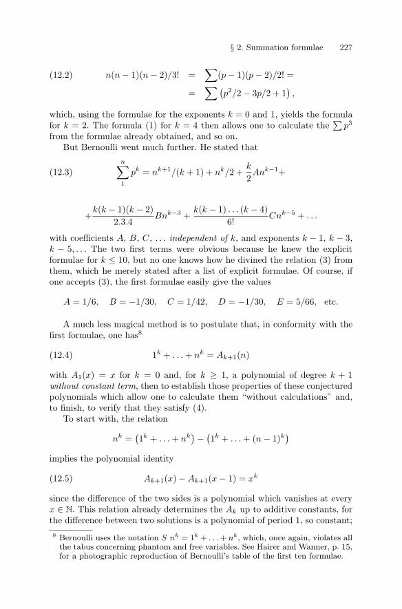
§ 2. Summation formulae 227
n(n − 1)(n − 2)/3! =∑
(p − 1)(p − 2)/2! =(12.2)
=∑(
p2/2 − 3p/2 + 1),
which, using the formulae for the exponents k = 0 and 1, yields the formulafor k = 2. The formula (1) for k = 4 then allows one to calculate the
∑p3
from the formulae already obtained, and so on.But Bernoulli went much further. He stated that
n∑1
pk = nk+1/(k + 1) + nk/2 +k
2Ank−1+(12.3)
+k(k − 1)(k − 2)
2.3.4Bnk−3 +
k(k − 1) . . . (k − 4)6!
Cnk−5 + . . .
with coefficients A, B, C, . . . independent of k, and exponents k − 1, k − 3,k − 5, . . . The two first terms were obvious because he knew the explicitformulae for k ≤ 10, but no one knows how he divined the relation (3) fromthem, which he merely stated after a list of explicit formulae. Of course, ifone accepts (3), the first formulae easily give the values
A = 1/6, B = −1/30, C = 1/42, D = −1/30, E = 5/66, etc.
A much less magical method is to postulate that, in conformity with thefirst formulae, one has8
1k + . . . + nk = Ak+1(n)(12.4)
with A1(x) = x for k = 0 and, for k ≥ 1, a polynomial of degree k + 1without constant term, then to establish those properties of these conjecturedpolynomials which allow one to calculate them “without calculations” and,to finish, to verify that they satisfy (4).
To start with, the relation
nk =(1k + . . . + nk
)− (1k + . . . + (n − 1)k)
implies the polynomial identity
Ak+1(x) − Ak+1(x − 1) = xk(12.5)
since the difference of the two sides is a polynomial which vanishes at everyx ∈ N. This relation already determines the Ak up to additive constants, forthe difference between two solutions is a polynomial of period 1, so constant;8 Bernoulli uses the notation S nk = 1k + . . . + nk, which, once again, violates all
the tabus concerning phantom and free variables. See Hairer and Wanner, p. 15,for a photographic reproduction of Bernoulli’s table of the first ten formulae.
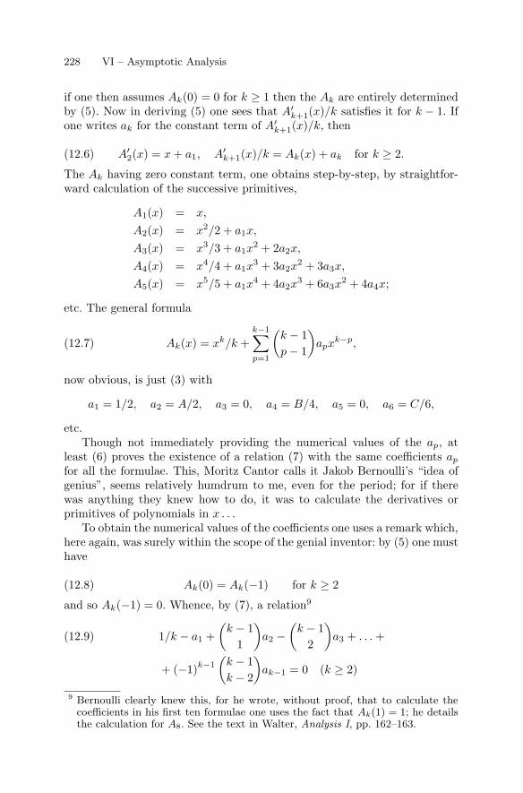
228 VI – Asymptotic Analysis
if one then assumes Ak(0) = 0 for k ≥ 1 then the Ak are entirely determinedby (5). Now in deriving (5) one sees that A′
k+1(x)/k satisfies it for k − 1. Ifone writes ak for the constant term of A′
k+1(x)/k, then
A′2(x) = x + a1, A′
k+1(x)/k = Ak(x) + ak for k ≥ 2.(12.6)
The Ak having zero constant term, one obtains step-by-step, by straightfor-ward calculation of the successive primitives,
A1(x) = x,
A2(x) = x2/2 + a1x,
A3(x) = x3/3 + a1x2 + 2a2x,
A4(x) = x4/4 + a1x3 + 3a2x
2 + 3a3x,
A5(x) = x5/5 + a1x4 + 4a2x
3 + 6a3x2 + 4a4x;
etc. The general formula
Ak(x) = xk/k +k−1∑p=1
(k − 1p − 1
)apx
k−p,(12.7)
now obvious, is just (3) with
a1 = 1/2, a2 = A/2, a3 = 0, a4 = B/4, a5 = 0, a6 = C/6,
etc.Though not immediately providing the numerical values of the ap, at
least (6) proves the existence of a relation (7) with the same coefficients ap
for all the formulae. This, Moritz Cantor calls it Jakob Bernoulli’s “idea ofgenius”, seems relatively humdrum to me, even for the period; for if therewas anything they knew how to do, it was to calculate the derivatives orprimitives of polynomials in x . . .
To obtain the numerical values of the coefficients one uses a remark which,here again, was surely within the scope of the genial inventor: by (5) one musthave
Ak(0) = Ak(−1) for k ≥ 2(12.8)
and so Ak(−1) = 0. Whence, by (7), a relation9
1/k − a1 +(
k − 11
)a2 −(
k − 12
)a3 + . . . +(12.9)
+ (−1)k−1
(k − 1k − 2
)ak−1 = 0 (k ≥ 2)
9 Bernoulli clearly knew this, for he wrote, without proof, that to calculate thecoefficients in his first ten formulae one uses the fact that Ak(1) = 1; he detailsthe calculation for A8. See the text in Walter, Analysis I, pp. 162–163.
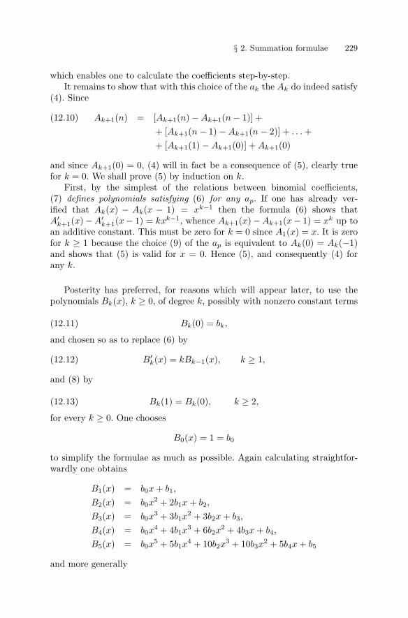
§ 2. Summation formulae 229
which enables one to calculate the coefficients step-by-step.It remains to show that with this choice of the ak the Ak do indeed satisfy
(4). Since
Ak+1(n) = [Ak+1(n) − Ak+1(n − 1)] +(12.10)+ [Ak+1(n − 1) − Ak+1(n − 2)] + . . . ++ [Ak+1(1) − Ak+1(0)] + Ak+1(0)
and since Ak+1(0) = 0, (4) will in fact be a consequence of (5), clearly truefor k = 0. We shall prove (5) by induction on k.
First, by the simplest of the relations between binomial coefficients,(7) defines polynomials satisfying (6) for any ap. If one has already ver-ified that Ak(x) − Ak(x − 1) = xk−1 then the formula (6) shows thatA′
k+1(x)−A′k+1(x− 1) = kxk−1, whence Ak+1(x)−Ak+1(x− 1) = xk up to
an additive constant. This must be zero for k = 0 since A1(x) = x. It is zerofor k ≥ 1 because the choice (9) of the ap is equivalent to Ak(0) = Ak(−1)and shows that (5) is valid for x = 0. Hence (5), and consequently (4) forany k.
Posterity has preferred, for reasons which will appear later, to use thepolynomials Bk(x), k ≥ 0, of degree k, possibly with nonzero constant terms
Bk(0) = bk,(12.11)
and chosen so as to replace (6) by
B′k(x) = kBk−1(x), k ≥ 1,(12.12)
and (8) by
Bk(1) = Bk(0), k ≥ 2,(12.13)
for every k ≥ 0. One chooses
B0(x) = 1 = b0
to simplify the formulae as much as possible. Again calculating straightfor-wardly one obtains
B1(x) = b0x + b1,
B2(x) = b0x2 + 2b1x + b2,
B3(x) = b0x3 + 3b1x
2 + 3b2x + b3,
B4(x) = b0x4 + 4b1x
3 + 6b2x2 + 4b3x + b4,
B5(x) = b0x5 + 5b1x
4 + 10b2x3 + 10b3x
2 + 5b4x + b5
and more generally
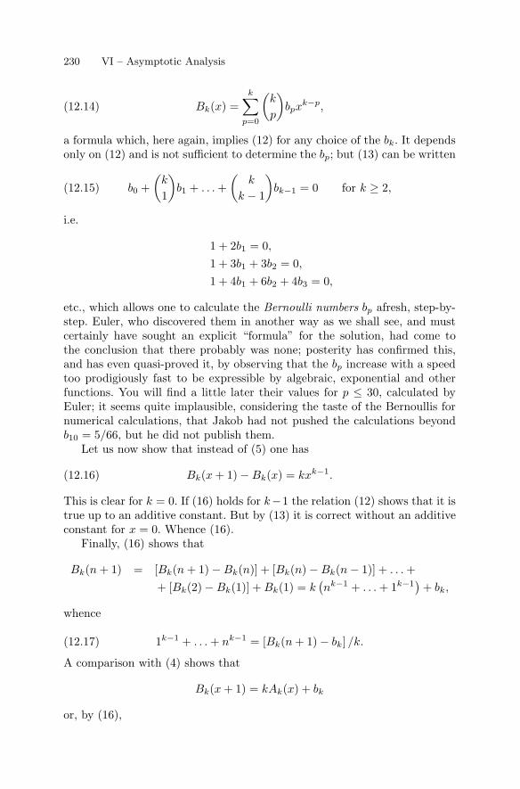
230 VI – Asymptotic Analysis
Bk(x) =k∑
p=0
(k
p
)bpx
k−p,(12.14)
a formula which, here again, implies (12) for any choice of the bk. It dependsonly on (12) and is not sufficient to determine the bp; but (13) can be written
b0 +(
k
1
)b1 + . . . +
(k
k − 1
)bk−1 = 0 for k ≥ 2,(12.15)
i.e.
1 + 2b1 = 0,1 + 3b1 + 3b2 = 0,1 + 4b1 + 6b2 + 4b3 = 0,
etc., which allows one to calculate the Bernoulli numbers bp afresh, step-by-step. Euler, who discovered them in another way as we shall see, and mustcertainly have sought an explicit “formula” for the solution, had come tothe conclusion that there probably was none; posterity has confirmed this,and has even quasi-proved it, by observing that the bp increase with a speedtoo prodigiously fast to be expressible by algebraic, exponential and otherfunctions. You will find a little later their values for p ≤ 30, calculated byEuler; it seems quite implausible, considering the taste of the Bernoullis fornumerical calculations, that Jakob had not pushed the calculations beyondb10 = 5/66, but he did not publish them.
Let us now show that instead of (5) one has
Bk(x + 1) − Bk(x) = kxk−1.(12.16)
This is clear for k = 0. If (16) holds for k−1 the relation (12) shows that it istrue up to an additive constant. But by (13) it is correct without an additiveconstant for x = 0. Whence (16).
Finally, (16) shows that
Bk(n + 1) = [Bk(n + 1) − Bk(n)] + [Bk(n) − Bk(n − 1)] + . . . ++ [Bk(2) − Bk(1)] + Bk(1) = k
(nk−1 + . . . + 1k−1
)+ bk,
whence
1k−1 + . . . + nk−1 = [Bk(n + 1) − bk] /k.(12.17)
A comparison with (4) shows that
Bk(x + 1) = kAk(x) + bk
or, by (16),
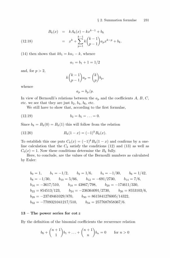
§ 2. Summation formulae 231
Bk(x) = kAk(x) − kxk−1 + bk
= xk +k−1∑p=1
k
(k − 1p − 1
)apx
k−p + bk.(12.18)
(14) then shows that kb1 = ka1 − k, whence
a1 = b1 + 1 = 1/2
and, for p > 2,
k
(k − 1p − 1
)ap =(
k
p
)bp,
whenceap = bp/p.
In view of Bernoulli’s relations between the ap and the coefficients A, B, C,etc. we see that they are just b2, b4, b6, etc.
We still have to show that, according to the first formulae,
b3 = b5 = . . . = 0.(12.19)
Since bk = Bk(0) = Bk(1) this will follow from the relation
Bk(1 − x) = (−1)kBk(x).(12.20)
To establish this one puts Ck(x) = (−1)kBk(1 − x) and confirms by a one-line calculation that the Ck satisfy the conditions (12) and (13) as well asC0(x) = 1. Now these conditions determine the Bk fully.
Here, to conclude, are the values of the Bernoulli numbers as calculatedby Euler:
b0 = 1, b1 = −1/2, b2 = 1/6, b4 = −1/30, b6 = 1/42,
b8 = −1/30, b10 = 5/66, b12 = −691/2730, b14 = 7/6,
b16 = −3617/510, b18 = 43867/798, b20 = −174611/330,
b22 = 854513/123, b24 = −236364091/2730, b26 = 8553103/6,
b28 = −23749461029/870, b30 = 8615841276005/14322,
b32 = −7709321041217/510, b34 = 2577687858367/6.
13 – The power series for cot z
By the definition of the binomial coefficients the recurrence relation
b0 +(
n + 11
)b1 + . . . +
(n + 1
n
)bn = 0 for n > 0
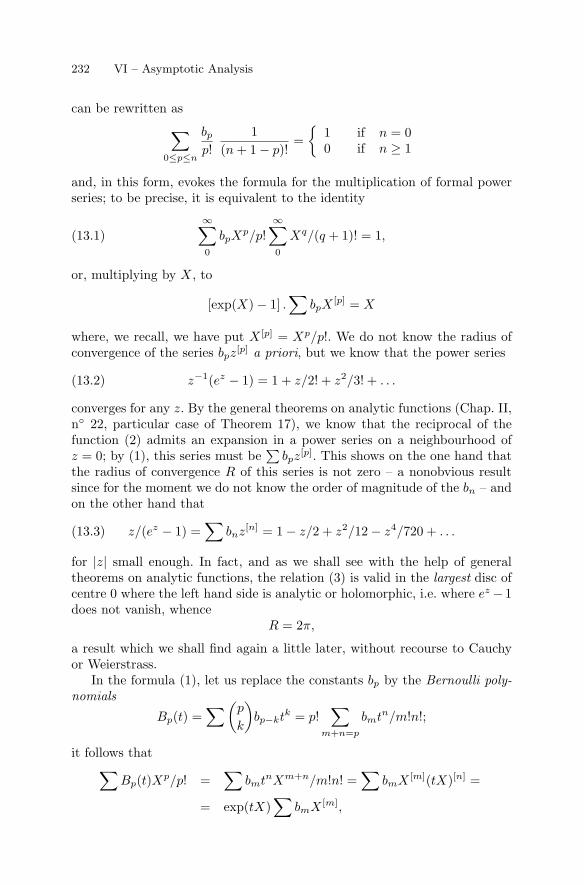
232 VI – Asymptotic Analysis
can be rewritten as∑0≤p≤n
bp
p!1
(n + 1 − p)!={
1 if n = 00 if n ≥ 1
and, in this form, evokes the formula for the multiplication of formal powerseries; to be precise, it is equivalent to the identity
∞∑0
bpXp/p!
∞∑0
Xq/(q + 1)! = 1,(13.1)
or, multiplying by X, to
[exp(X) − 1] .∑
bpX[p] = X
where, we recall, we have put X [p] = Xp/p!. We do not know the radius ofconvergence of the series bpz
[p] a priori, but we know that the power series
z−1(ez − 1) = 1 + z/2! + z2/3! + . . .(13.2)
converges for any z. By the general theorems on analytic functions (Chap. II,n◦ 22, particular case of Theorem 17), we know that the reciprocal of thefunction (2) admits an expansion in a power series on a neighbourhood ofz = 0; by (1), this series must be
∑bpz
[p]. This shows on the one hand thatthe radius of convergence R of this series is not zero – a nonobvious resultsince for the moment we do not know the order of magnitude of the bn – andon the other hand that
z/(ez − 1) =∑
bnz[n] = 1 − z/2 + z2/12 − z4/720 + . . .(13.3)
for |z| small enough. In fact, and as we shall see with the help of generaltheorems on analytic functions, the relation (3) is valid in the largest disc ofcentre 0 where the left hand side is analytic or holomorphic, i.e. where ez −1does not vanish, whence
R = 2π,
a result which we shall find again a little later, without recourse to Cauchyor Weierstrass.
In the formula (1), let us replace the constants bp by the Bernoulli poly-nomials
Bp(t) =∑(p
k
)bp−ktk = p!
∑m+n=p
bmtn/m!n!;
it follows that∑Bp(t)Xp/p! =
∑bmtnXm+n/m!n! =
∑bmX [m](tX)[n] =
= exp(tX)∑
bmX [m],
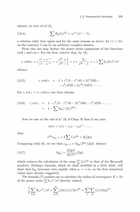
§ 2. Summation formulae 233
whence, in view of of (3),∑Bp(t)z[p] = zetz/(ez − 1),(13.4)
a relation valid, here again and for the same reasons as above, for |z| < 2π;on the contrary, t can be an arbitrary complex number.
From this one may deduce the power series expansions of the functionscoth z and cot z. For the first, observe that, by (3),
z. coth z = z.ez + e−z
ez − e−z= z.
e2z + 1e2z − 1
= z +2z
e2z − 1= z +∑
bn(2z)n/n!
whence
z. coth z = 1 + z2/3 − z4/45 + 2z6/945 −(13.5)− z8/4725 + 2z10/18711 − . . . .
For z. cot z = iz. coth iz one then obtains
z. cot z = 1 − z2/3 − z4/45 − 2z6/945 − z8/4725 − . . . ,(13.6)
= 1 −∑
|b2n| (2z)[2n].
Now we saw at the end of n◦ 22 of Chap. II that if one puts
cot x = 1/x − c1x − c3x3 − . . . ,
thenπ2pc2p−1 = 2
∑1/n2p = 2ζ(2p).
Comparing with (6), we see that c2p−1 = |b2p| 22p/(2p)!, whence
|b2p| =2(2p)!(2π)2p
ζ(2p),(13.7)
which reduces the calculation of the sums∑
1/n2p to that of the Bernoullinumbers. Stirling’s formula, which we shall establish in a little while, willshow that b2p increases very rapidly when p → +∞, as the first numericalvalues have already suggested.
The formula (7) enables one to calculate the radius of convergence R = 2πof the power series
∑bnzn/n! directly; indeed,
12
∑n≥2
|bnzn| /n! =∞∑
n=2
ζ(2n) (|z|/2π)2n =∑
n
∑p
(|z|/2πp)2n,
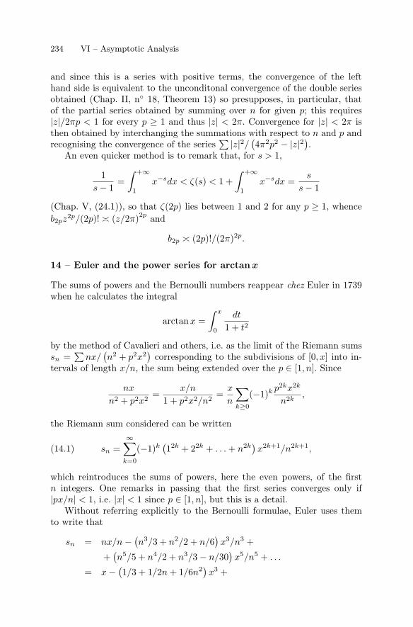
234 VI – Asymptotic Analysis
and since this is a series with positive terms, the convergence of the lefthand side is equivalent to the unconditonal convergence of the double seriesobtained (Chap. II, n◦ 18, Theorem 13) so presupposes, in particular, thatof the partial series obtained by summing over n for given p; this requires|z|/2πp < 1 for every p ≥ 1 and thus |z| < 2π. Convergence for |z| < 2π isthen obtained by interchanging the summations with respect to n and p andrecognising the convergence of the series
∑ |z|2/ (4π2p2 − |z|2).An even quicker method is to remark that, for s > 1,
1s − 1
=∫ +∞
1
x−sdx < ζ(s) < 1 +∫ +∞
1
x−sdx =s
s − 1
(Chap. V, (24.1)), so that ζ(2p) lies between 1 and 2 for any p ≥ 1, whenceb2pz
2p/(2p)! � (z/2π)2p and
b2p � (2p)!/(2π)2p.
14 – Euler and the power series for arctan x
The sums of powers and the Bernoulli numbers reappear chez Euler in 1739when he calculates the integral
arctanx =∫ x
0
dt
1 + t2
by the method of Cavalieri and others, i.e. as the limit of the Riemann sumssn =∑
nx/(n2 + p2x2
)corresponding to the subdivisions of [0, x] into in-
tervals of length x/n, the sum being extended over the p ∈ [1, n]. Since
nx
n2 + p2x2=
x/n
1 + p2x2/n2=
x
n
∑k≥0
(−1)k p2kx2k
n2k,
the Riemann sum considered can be written
sn =∞∑
k=0
(−1)k(12k + 22k + . . . + n2k
)x2k+1/n2k+1,(14.1)
which reintroduces the sums of powers, here the even powers, of the firstn integers. One remarks in passing that the first series converges only if|px/n| < 1, i.e. |x| < 1 since p ∈ [1, n], but this is a detail.
Without referring explicitly to the Bernoulli formulae, Euler uses themto write that
sn = nx/n − (n3/3 + n2/2 + n/6)x3/n3 +
+(n5/5 + n4/2 + n3/3 − n/30
)x5/n5 + . . .
= x − (1/3 + 1/2n + 1/6n2)x3 +
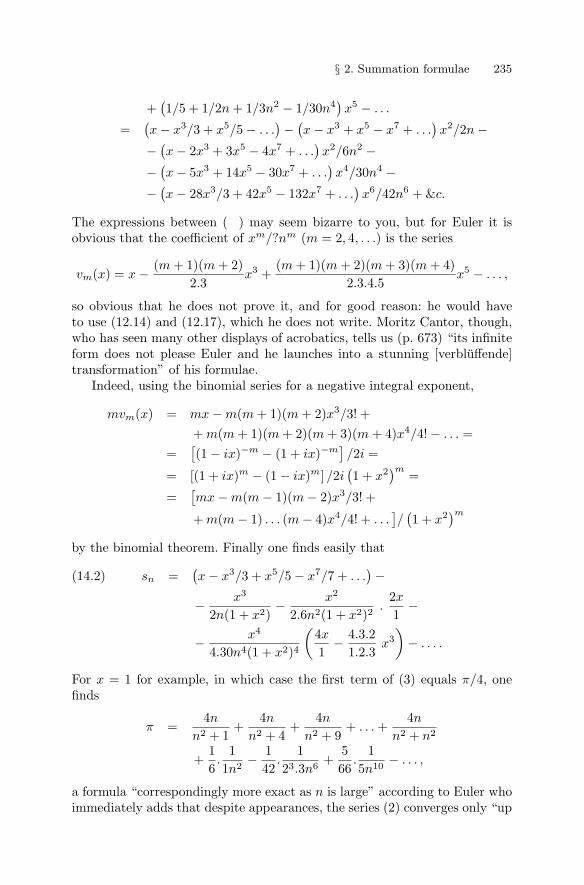
§ 2. Summation formulae 235
+(1/5 + 1/2n + 1/3n2 − 1/30n4
)x5 − . . .
=(x − x3/3 + x5/5 − . . .
)− (x − x3 + x5 − x7 + . . .)x2/2n −
− (x − 2x3 + 3x5 − 4x7 + . . .)x2/6n2 −
− (x − 5x3 + 14x5 − 30x7 + . . .)x4/30n4 −
− (x − 28x3/3 + 42x5 − 132x7 + . . .)x6/42n6 + &c.
The expressions between ( ) may seem bizarre to you, but for Euler it isobvious that the coefficient of xm/?nm (m = 2, 4, . . .) is the series
vm(x) = x − (m + 1)(m + 2)2.3
x3 +(m + 1)(m + 2)(m + 3)(m + 4)
2.3.4.5x5 − . . . ,
so obvious that he does not prove it, and for good reason: he would haveto use (12.14) and (12.17), which he does not write. Moritz Cantor, though,who has seen many other displays of acrobatics, tells us (p. 673) “its infiniteform does not please Euler and he launches into a stunning [verbluffende]transformation” of his formulae.
Indeed, using the binomial series for a negative integral exponent,
mvm(x) = mx − m(m + 1)(m + 2)x3/3! ++ m(m + 1)(m + 2)(m + 3)(m + 4)x4/4! − . . . =
=[(1 − ix)−m − (1 + ix)−m
]/2i =
= [(1 + ix)m − (1 − ix)m] /2i(1 + x2)m
=
=[mx − m(m − 1)(m − 2)x3/3! +
+ m(m − 1) . . . (m − 4)x4/4! + . . .]/(1 + x2)m
by the binomial theorem. Finally one finds easily that
sn =(x − x3/3 + x5/5 − x7/7 + . . .
)−(14.2)
− x3
2n(1 + x2)− x2
2.6n2(1 + x2)2.
2x
1−
− x4
4.30n4(1 + x2)4
(4x
1− 4.3.2
1.2.3x3
)− . . . .
For x = 1 for example, in which case the first term of (3) equals π/4, onefinds
π =4n
n2 + 1+
4n
n2 + 4+
4n
n2 + 9+ . . . +
4n
n2 + n2
+16.
11n2
− 142
.1
23.3n6+
566
.1
5n10− . . . ,
a formula “correspondingly more exact as n is large” according to Euler whoimmediately adds that despite appearances, the series (2) converges only “up
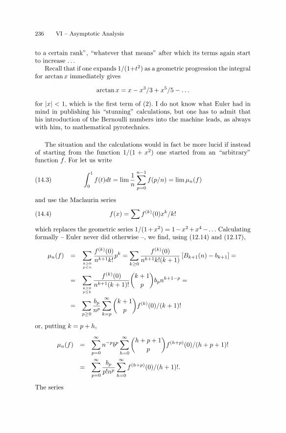
236 VI – Asymptotic Analysis
to a certain rank”, “whatever that means” after which its terms again startto increase . . .
Recall that if one expands 1/(1+t2) as a geometric progression the integralfor arctanx immediately gives
arctan x = x − x3/3 + x5/5 − . . .
for |x| < 1, which is the first term of (2). I do not know what Euler had inmind in publishing his “stunning” calculations, but one has to admit thathis introduction of the Bernoulli numbers into the machine leads, as alwayswith him, to mathematical pyrotechnics.
The situation and the calculations would in fact be more lucid if insteadof starting from the function 1/(1 + x2) one started from an “arbitrary”function f . For let us write
∫ 1
0
f(t)dt = lim1n
n−1∑p=0
f(p/n) = limµn(f)(14.3)
and use the Maclaurin series
f(x) =∑
f (k)(0)xk/k!(14.4)
which replaces the geometric series 1/(1+x2) = 1−x2 +x4− . . . Calculatingformally – Euler never did otherwise –, we find, using (12.14) and (12.17),
µn(f) =∑k≥0p<n
f (k)(0)nk+1k!
pk =∑k≥0
f (k)(0)nk+1k!(k + 1)
[Bk+1(n) − bk+1] =
=∑k≥0p≤k
f (k)(0)nk+1(k + 1)!
(k + 1
p
)bpn
k+1−p =
=∑p≥0
bp
np
∞∑k=p
(k + 1
p
)f (k)(0)/(k + 1)!
or, putting k = p + h,
µn(f) =∞∑
p=0
n−pbp∞∑
h=0
(h + p + 1
p
)f (h+p)(0)/(h + p + 1)!
=∞∑
p=0
bp
p!np
∞∑h=0
f (h+p)(0)/(h + 1)!.
The series
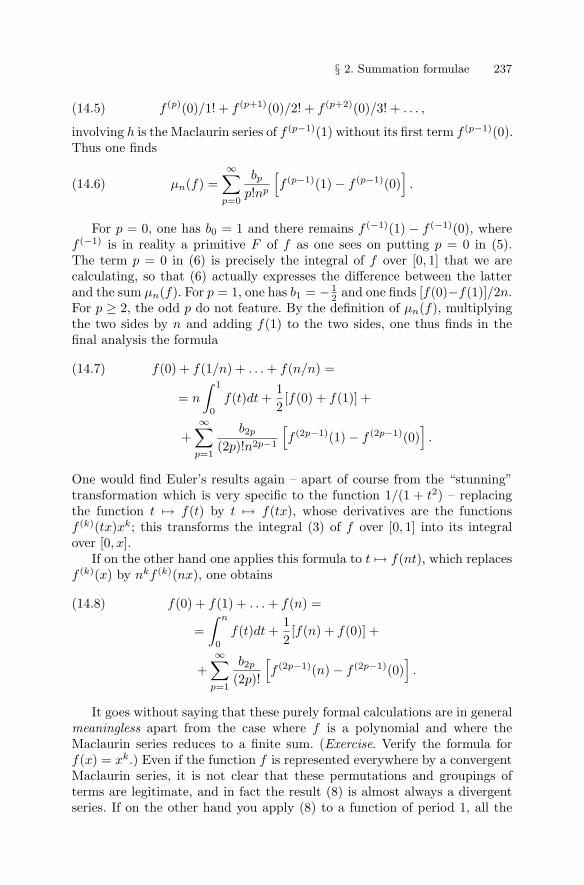
§ 2. Summation formulae 237
f (p)(0)/1! + f (p+1)(0)/2! + f (p+2)(0)/3! + . . . ,(14.5)
involving h is the Maclaurin series of f (p−1)(1) without its first term f (p−1)(0).Thus one finds
µn(f) =∞∑
p=0
bp
p!np
[f (p−1)(1) − f (p−1)(0)
].(14.6)
For p = 0, one has b0 = 1 and there remains f (−1)(1) − f (−1)(0), wheref (−1) is in reality a primitive F of f as one sees on putting p = 0 in (5).The term p = 0 in (6) is precisely the integral of f over [0, 1] that we arecalculating, so that (6) actually expresses the difference between the latterand the sum µn(f). For p = 1, one has b1 = − 1
2 and one finds [f(0)−f(1)]/2n.For p ≥ 2, the odd p do not feature. By the definition of µn(f), multiplyingthe two sides by n and adding f(1) to the two sides, one thus finds in thefinal analysis the formula
f(0) + f(1/n) + . . . + f(n/n) =(14.7)
= n
∫ 1
0
f(t)dt +12[f(0) + f(1)] +
+∞∑
p=1
b2p
(2p)!n2p−1
[f (2p−1)(1) − f (2p−1)(0)
].
One would find Euler’s results again – apart of course from the “stunning”transformation which is very specific to the function 1/(1 + t2) – replacingthe function t → f(t) by t → f(tx), whose derivatives are the functionsf (k)(tx)xk; this transforms the integral (3) of f over [0, 1] into its integralover [0, x].
If on the other hand one applies this formula to t → f(nt), which replacesf (k)(x) by nkf (k)(nx), one obtains
f(0) + f(1) + . . . + f(n) =(14.8)
=∫ n
0
f(t)dt +12[f(n) + f(0)] +
+∞∑
p=1
b2p
(2p)!
[f (2p−1)(n) − f (2p−1)(0)
].
It goes without saying that these purely formal calculations are in generalmeaningless apart from the case where f is a polynomial and where theMaclaurin series reduces to a finite sum. (Exercise. Verify the formula forf(x) = xk.) Even if the function f is represented everywhere by a convergentMaclaurin series, it is not clear that these permutations and groupings ofterms are legitimate, and in fact the result (8) is almost always a divergentseries. If on the other hand you apply (8) to a function of period 1, all the
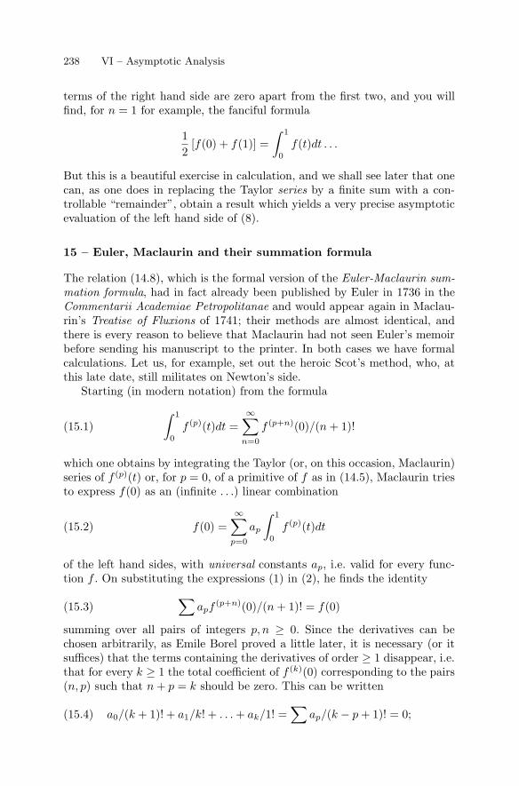
238 VI – Asymptotic Analysis
terms of the right hand side are zero apart from the first two, and you willfind, for n = 1 for example, the fanciful formula
12
[f(0) + f(1)] =∫ 1
0
f(t)dt . . .
But this is a beautiful exercise in calculation, and we shall see later that onecan, as one does in replacing the Taylor series by a finite sum with a con-trollable “remainder”, obtain a result which yields a very precise asymptoticevaluation of the left hand side of (8).
15 – Euler, Maclaurin and their summation formula
The relation (14.8), which is the formal version of the Euler-Maclaurin sum-mation formula, had in fact already been published by Euler in 1736 in theCommentarii Academiae Petropolitanae and would appear again in Maclau-rin’s Treatise of Fluxions of 1741; their methods are almost identical, andthere is every reason to believe that Maclaurin had not seen Euler’s memoirbefore sending his manuscript to the printer. In both cases we have formalcalculations. Let us, for example, set out the heroic Scot’s method, who, atthis late date, still militates on Newton’s side.
Starting (in modern notation) from the formula
∫ 1
0
f (p)(t)dt =∞∑
n=0
f (p+n)(0)/(n + 1)!(15.1)
which one obtains by integrating the Taylor (or, on this occasion, Maclaurin)series of f (p)(t) or, for p = 0, of a primitive of f as in (14.5), Maclaurin triesto express f(0) as an (infinite . . .) linear combination
f(0) =∞∑
p=0
ap
∫ 1
0
f (p)(t)dt(15.2)
of the left hand sides, with universal constants ap, i.e. valid for every func-tion f . On substituting the expressions (1) in (2), he finds the identity∑
apf(p+n)(0)/(n + 1)! = f(0)(15.3)
summing over all pairs of integers p, n ≥ 0. Since the derivatives can bechosen arbitrarily, as Emile Borel proved a little later, it is necessary (or itsuffices) that the terms containing the derivatives of order ≥ 1 disappear, i.e.that for every k ≥ 1 the total coefficient of f (k)(0) corresponding to the pairs(n, p) such that n + p = k should be zero. This can be written
a0/(k + 1)! + a1/k! + . . . + ak/1! =∑
ap/(k − p + 1)! = 0;(15.4)
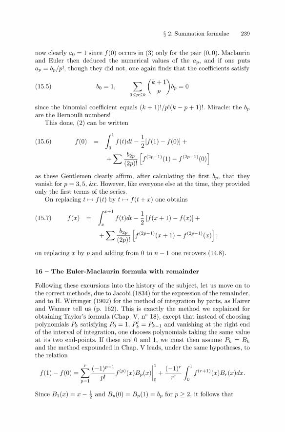
§ 2. Summation formulae 239
now clearly a0 = 1 since f(0) occurs in (3) only for the pair (0, 0). Maclaurinand Euler then deduced the numerical values of the ap, and if one putsap = bp/p!, though they did not, one again finds that the coefficients satisfy
b0 = 1,∑
0≤p≤k
(k + 1
p
)bp = 0(15.5)
since the binomial coefficient equals (k + 1)!/p!(k − p + 1)!. Miracle: the bp
are the Bernoulli numbers!This done, (2) can be written
f(0) =∫ 1
0
f(t)dt − 12[f(1) − f(0)] +(15.6)
+∑ b2p
(2p)!
[f (2p−1)(1) − f (2p−1)(0)
]as these Gentlemen clearly affirm, after calculating the first bp, that theyvanish for p = 3, 5, &c. However, like everyone else at the time, they providedonly the first terms of the series.
On replacing t → f(t) by t → f(t + x) one obtains
f(x) =∫ x+1
x
f(t)dt − 12
[f(x + 1) − f(x)] +(15.7)
+∑ b2p
(2p)!
[f (2p−1)(x + 1) − f (2p−1)(x)
];
on replacing x by p and adding from 0 to n − 1 one recovers (14.8).
16 – The Euler-Maclaurin formula with remainder
Following these excursions into the history of the subject, let us move on tothe correct methods, due to Jacobi (1834) for the expression of the remainder,and to H. Wirtinger (1902) for the method of integration by parts, as Hairerand Wanner tell us (p. 162). This is exactly the method we explained forobtaining Taylor’s formula (Chap. V, n◦ 18), except that instead of choosingpolynomials Pk satisfying P0 = 1, P ′
k = Pk−1 and vanishing at the right endof the interval of integration, one chooses polynomials taking the same valueat its two end-points. If these are 0 and 1, we must then assume Pk = Bk
and the method expounded in Chap. V leads, under the same hypotheses, tothe relation
f(1) − f(0) =r∑
p=1
(−1)p−1
p!f (p)(x)Bp(x)
∣∣∣∣10
+(−1)r
r!
∫ 1
0
f (r+1)(x)Br(x)dx.
Since B1(x) = x − 12 and Bp(0) = Bp(1) = bp for p ≥ 2, it follows that
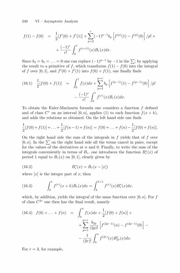
240 VI – Asymptotic Analysis
f(1) − f(0) =12[f ′(0) + f ′(1)] +
r∑p=2
(−1)p−1bp
[f (p)(1) − f (p)(0)
]/p! +
+(−1)r
r!
∫ 1
0
f (r+1)(x)Br(x)dx.
Since b3 = b5 = . . . = 0 one can replace (−1)p−1 by −1 in the∑
; by applyingthe result to a primitive of f , which transforms f(1)− f(0) into the integralof f over [0, 1], and f ′(0) + f ′(1) into f(0) + f(1), one finally finds
12[f(0) + f(1)] =
∫ 1
0
f(x)dx +p=r∑p=2
bp
[f (p−1)(1) − f (p−1)(0)
]/p!(16.1)
− (−1)r
r!
∫ 1
0
f (r)(x)Br(x)dx.
To obtain the Euler-Maclaurin formula one considers a function f definedand of class Cr on an interval [0, n], applies (1) to each function f(x + k),and adds the relations so obtained. On the left hand side one finds
12[f(0)+f(1)]+ . . .+
12[f(n−1)+f(n)] = f(0)+ . . .+f(n)− 1
2[f(0)+f(n)].
On the right hand side the sum of the integrals in f yields that of f over[0, n]. In the
∑on the right hand side all the terms cancel in pairs, except
for the values of the derivatives at n and 0. Finally, to write the sum of theintegrals conveniently in terms of Br, one introduces the function B∗
r (x) ofperiod 1 equal to Br(x) on [0, 1], clearly given by
B∗r (x) = Br(x − [x])(16.2)
where [x] is the integer part of x; then∫ 1
0
f (r)(x + k)Br(x)dx =∫ k+1
k
f (r)(x)B∗r (x)dx,(16.3)
which, by addition, yields the integral of the same function over [0, n]. For fof class C2r one then has the final result, namely
f(0) + . . . + f(n) =∫ n
0
f(x)dx +12[f(0) + f(n)] +(16.4)
+p=r∑p=1
b2p
(2p)!
[f (2p−1)(n) − f (2p−1)(0)
]−
− 1(2r)!
∫ n
0
f (2r)(x)B∗2r(x)dx.
For r = 3, for example,
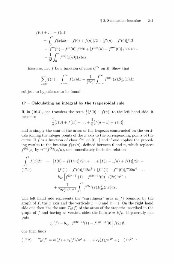
§ 2. Summation formulae 241
f(0) + . . . + f(n) =
=∫ n
0
f(x)dx + [f(0) + f(n)]/2 + [f ′(n) − f ′(0)]/12 −− [f ′′′(n) − f ′′′(0)] /720 + [f ′′′′′(n) − f ′′′′′(0)] /30240 −− 1
6!
∫ n
0
f (6)(x)B∗6(x)dx.
Exercise. Let f be a function of class C2r on R. Show that
∑n∈Z
f(n) =∫ ∞
−∞f(x)dx − 1
(2r)!
∫ ∞
−∞f (2r)(x)B∗
2r(x)dx
subject to hypotheses to be found.
17 – Calculating an integral by the trapezoidal rule
If, in (16.4), one transfers the term 12 [f(0) + f(n)] to the left hand side, it
becomes12[f(0) + f(1)] + . . . +
12[f(n − 1) + f(n)]
and is simply the sum of the areas of the trapezia constructed on the verti-cals joining the integer points of the x axis to the corresponding points of thecurve. If f is a function of class C2r on [0, 1] and if one applies the preced-ing results to the function f(x/n), defined between 0 and n, which replacesf (k)(x) by n−kf (k)(x/n), one immediately finds the relation∫ 1
0
f(x)dx = [f(0) + f(1/n)]/2n + . . . + [f(1 − 1/n) + f(1)]/2n −
− [f ′(1) − f ′(0)]/12n2 + [f ′′′(1) − f ′′′(0)]/720n4 − . . . −(17.1)
− b2r
[f (2r−1)(1) − f (2r−1)(0)
]/(2r)!n2r +
+1
(2r)!n2r+1
∫ 1
0
f (2r)(x)B∗2r(nx)dx.
The left hand side represents the “curvilinear” area m(f) bounded by thegraph of f , the x axis and the verticals x = 0 and x = 1. On the right handside one then has the sum Tn(f) of the areas of the trapezia inscribed in thegraph of f and having as vertical sides the lines x = k/n. If generally oneputs
cp(f) = b2p
[f (2p−1)(1) − f (2p−1)(0)
]/(2p)!,
one then finds
Tn(f) = m(f) + c1(f)/n2 + . . . + cr(f)/n2r + (. . .)/n2r+1(17.2)
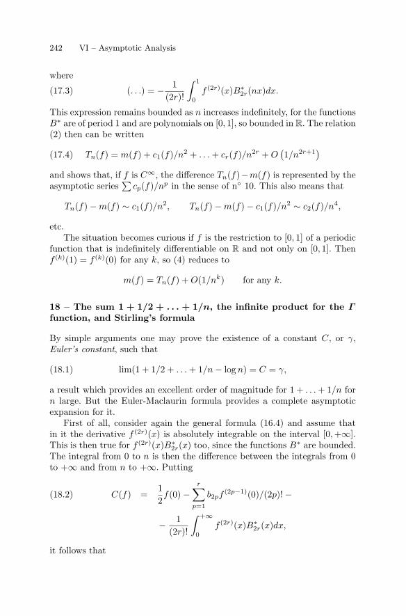
242 VI – Asymptotic Analysis
where
(. . .) = − 1(2r)!
∫ 1
0
f (2r)(x)B∗2r(nx)dx.(17.3)
This expression remains bounded as n increases indefinitely, for the functionsB∗ are of period 1 and are polynomials on [0, 1], so bounded in R. The relation(2) then can be written
Tn(f) = m(f) + c1(f)/n2 + . . . + cr(f)/n2r + O(1/n2r+1
)(17.4)
and shows that, if f is C∞, the difference Tn(f)−m(f) is represented by theasymptotic series
∑cp(f)/np in the sense of n◦ 10. This also means that
Tn(f) − m(f) ∼ c1(f)/n2, Tn(f) − m(f) − c1(f)/n2 ∼ c2(f)/n4,
etc.The situation becomes curious if f is the restriction to [0, 1] of a periodic
function that is indefinitely differentiable on R and not only on [0, 1]. Thenf (k)(1) = f (k)(0) for any k, so (4) reduces to
m(f) = Tn(f) + O(1/nk) for any k.
18 – The sum 1 + 1/2 + . . . + 1/n, the infinite product for the Γfunction, and Stirling’s formula
By simple arguments one may prove the existence of a constant C, or γ,Euler’s constant, such that
lim(1 + 1/2 + . . . + 1/n − log n) = C = γ,(18.1)
a result which provides an excellent order of magnitude for 1 + . . . + 1/n forn large. But the Euler-Maclaurin formula provides a complete asymptoticexpansion for it.
First of all, consider again the general formula (16.4) and assume thatin it the derivative f (2r)(x) is absolutely integrable on the interval [0,+∞].This is then true for f (2r)(x)B∗
2r(x) too, since the functions B∗ are bounded.The integral from 0 to n is then the difference between the integrals from 0to +∞ and from n to +∞. Putting
C(f) =12f(0) −
r∑p=1
b2pf(2p−1)(0)/(2p)! −(18.2)
− 1(2r)!
∫ +∞
0
f (2r)(x)B∗2r(x)dx,
it follows that
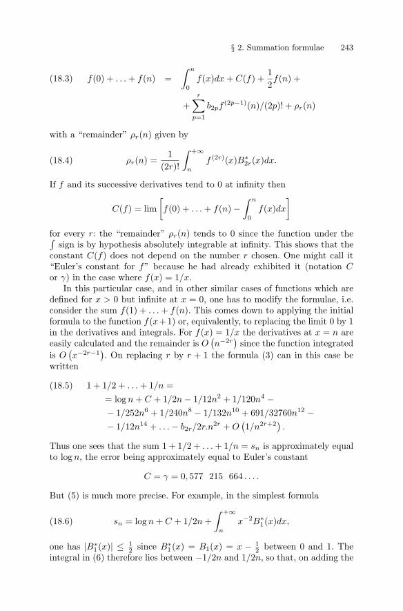
§ 2. Summation formulae 243
f(0) + . . . + f(n) =∫ n
0
f(x)dx + C(f) +12f(n) +(18.3)
+r∑
p=1
b2pf(2p−1)(n)/(2p)! + ρr(n)
with a “remainder” ρr(n) given by
ρr(n) =1
(2r)!
∫ +∞
n
f (2r)(x)B∗2r(x)dx.(18.4)
If f and its successive derivatives tend to 0 at infinity then
C(f) = lim[f(0) + . . . + f(n) −
∫ n
0
f(x)dx
]
for every r: the “remainder” ρr(n) tends to 0 since the function under the∫sign is by hypothesis absolutely integrable at infinity. This shows that the
constant C(f) does not depend on the number r chosen. One might call it“Euler’s constant for f” because he had already exhibited it (notation Cor γ) in the case where f(x) = 1/x.
In this particular case, and in other similar cases of functions which aredefined for x > 0 but infinite at x = 0, one has to modify the formulae, i.e.consider the sum f(1) + . . . + f(n). This comes down to applying the initialformula to the function f(x+1) or, equivalently, to replacing the limit 0 by 1in the derivatives and integrals. For f(x) = 1/x the derivatives at x = n areeasily calculated and the remainder is O
(n−2r)
since the function integratedis O(x−2r−1
). On replacing r by r + 1 the formula (3) can in this case be
written
1 + 1/2 + . . . + 1/n =(18.5)= log n + C + 1/2n − 1/12n2 + 1/120n4 −− 1/252n6 + 1/240n8 − 1/132n10 + 691/32760n12 −− 1/12n14 + . . . − b2r/2r.n2r + O
(1/n2r+2
).
Thus one sees that the sum 1 + 1/2 + . . . + 1/n = sn is approximately equalto log n, the error being approximately equal to Euler’s constant
C = γ = 0, 577 215 664 . . . .
But (5) is much more precise. For example, in the simplest formula
sn = log n + C + 1/2n +∫ +∞
n
x−2B∗1(x)dx,(18.6)
one has |B∗1(x)| ≤ 1
2 since B∗1(x) = B1(x) = x − 1
2 between 0 and 1. Theintegral in (6) therefore lies between −1/2n and 1/2n, so that, on adding the
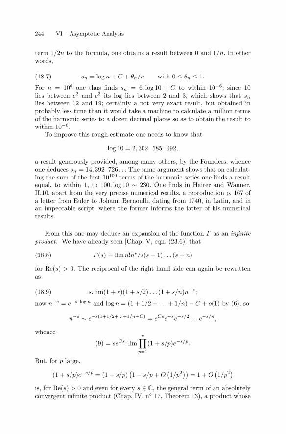
244 VI – Asymptotic Analysis
term 1/2n to the formula, one obtains a result between 0 and 1/n. In otherwords,
sn = log n + C + θn/n with 0 ≤ θn ≤ 1.(18.7)
For n = 106 one thus finds sn = 6. log 10 + C to within 10−6; since 10lies between e2 and e3 its log lies between 2 and 3, which shows that sn
lies between 12 and 19; certainly a not very exact result, but obtained inprobably less time than it would take a machine to calculate a million termsof the harmonic series to a dozen decimal places so as to obtain the result towithin 10−6.
To improve this rough estimate one needs to know that
log 10 = 2, 302 585 092,
a result generously provided, among many others, by the Founders, whenceone deduces sn = 14, 392 726 . . . The same argument shows that on calculat-ing the sum of the first 10100 terms of the harmonic series one finds a resultequal, to within 1, to 100. log 10 ∼ 230. One finds in Hairer and Wanner,II.10, apart from the very precise numerical results, a reproduction p. 167 ofa letter from Euler to Johann Bernoulli, dating from 1740, in Latin, and inan impeccable script, where the former informs the latter of his numericalresults.
From this one may deduce an expansion of the function Γ as an infiniteproduct. We have already seen [Chap. V, eqn. (23.6)] that
Γ (s) = limn!ns/s(s + 1) . . . (s + n)(18.8)
for Re(s) > 0. The reciprocal of the right hand side can again be rewrittenas
s. lim(1 + s)(1 + s/2) . . . (1 + s/n)n−s;(18.9)
now n−s = e−s. log n and log n = (1 + 1/2 + . . . + 1/n) − C + o(1) by (6); so
n−s ∼ e−s(1+1/2+...+1/n−C) = eCse−se−s/2 . . . e−s/n,
whence
(9) = seCs. limn∏
p=1
(1 + s/p)e−s/p.
But, for p large,
(1 + s/p)e−s/p = (1 + s/p)(1 − s/p + O
(1/p2))
= 1 + O(1/p2)
is, for Re(s) > 0 and even for every s ∈ C, the general term of an absolutelyconvergent infinite product (Chap. IV, n◦ 17, Theorem 13), a product whose
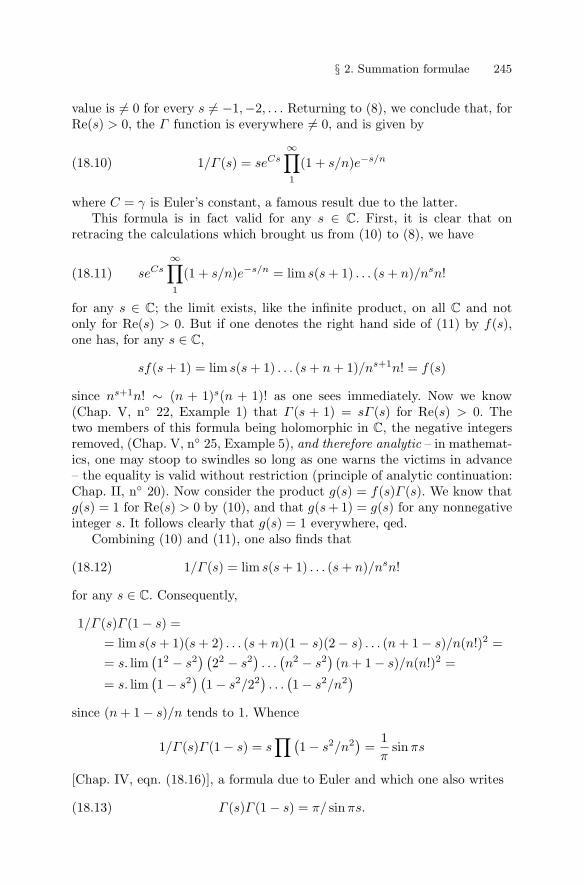
§ 2. Summation formulae 245
value is �= 0 for every s �= −1,−2, . . . Returning to (8), we conclude that, forRe(s) > 0, the Γ function is everywhere �= 0, and is given by
1/Γ (s) = seCs∞∏1
(1 + s/n)e−s/n(18.10)
where C = γ is Euler’s constant, a famous result due to the latter.This formula is in fact valid for any s ∈ C. First, it is clear that on
retracing the calculations which brought us from (10) to (8), we have
seCs∞∏1
(1 + s/n)e−s/n = lim s(s + 1) . . . (s + n)/nsn!(18.11)
for any s ∈ C; the limit exists, like the infinite product, on all C and notonly for Re(s) > 0. But if one denotes the right hand side of (11) by f(s),one has, for any s ∈ C,
sf(s + 1) = lim s(s + 1) . . . (s + n + 1)/ns+1n! = f(s)
since ns+1n! ∼ (n + 1)s(n + 1)! as one sees immediately. Now we know(Chap. V, n◦ 22, Example 1) that Γ (s + 1) = sΓ (s) for Re(s) > 0. Thetwo members of this formula being holomorphic in C, the negative integersremoved, (Chap. V, n◦ 25, Example 5), and therefore analytic – in mathemat-ics, one may stoop to swindles so long as one warns the victims in advance– the equality is valid without restriction (principle of analytic continuation:Chap. II, n◦ 20). Now consider the product g(s) = f(s)Γ (s). We know thatg(s) = 1 for Re(s) > 0 by (10), and that g(s + 1) = g(s) for any nonnegativeinteger s. It follows clearly that g(s) = 1 everywhere, qed.
Combining (10) and (11), one also finds that
1/Γ (s) = lim s(s + 1) . . . (s + n)/nsn!(18.12)
for any s ∈ C. Consequently,
1/Γ (s)Γ (1 − s) == lim s(s + 1)(s + 2) . . . (s + n)(1 − s)(2 − s) . . . (n + 1 − s)/n(n!)2 == s. lim
(12 − s2
) (22 − s2
). . .(n2 − s2
)(n + 1 − s)/n(n!)2 =
= s. lim(1 − s2) (
1 − s2/22). . .(1 − s2/n2
)since (n + 1 − s)/n tends to 1. Whence
1/Γ (s)Γ (1 − s) = s∏(
1 − s2/n2)
=1π
sin πs
[Chap. IV, eqn. (18.16)], a formula due to Euler and which one also writes
Γ (s)Γ (1 − s) = π/ sin πs.(18.13)
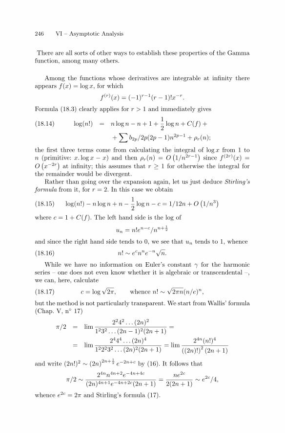
246 VI – Asymptotic Analysis
There are all sorts of other ways to establish these properties of the Gammafunction, among many others.
Among the functions whose derivatives are integrable at infinity thereappears f(x) = log x, for which
f (r)(x) = (−1)r−1(r − 1)!x−r.
Formula (18.3) clearly applies for r > 1 and immediately gives
log(n!) = n log n − n + 1 +12
log n + C(f) +(18.14)
+∑
b2p/2p(2p − 1)n2p−1 + ρr(n);
the first three terms come from calculating the integral of log x from 1 ton (primitive: x. log x − x) and then ρr(n) = O
(1/n2r−1
)since f (2r)(x) =
O(x−2r)
at infinity; this assumes that r ≥ 1 for otherwise the integral forthe remainder would be divergent.
Rather than going over the expansion again, let us just deduce Stirling’sformula from it, for r = 2. In this case we obtain
log(n!) − n log n + n − 12
log n − c = 1/12n + O(1/n3)
(18.15)
where c = 1 + C(f). The left hand side is the log of
un = n!en−c/nn+ 12
and since the right hand side tends to 0, we see that un tends to 1, whence
n! ∼ ecnne−n√
n.(18.16)
While we have no information on Euler’s constant γ for the harmonicseries – one does not even know whether it is algebraic or transcendental –,we can, here, calculate
c = log√
2π, whence n! ∼√
2πn(n/e)n,(18.17)
but the method is not particularly transparent. We start from Wallis’ formula(Chap. V, n◦ 17)
π/2 = lim2242 . . . (2n)2
1232 . . . (2n − 1)2(2n + 1)=
= lim2444 . . . (2n)4
122232 . . . (2n)2(2n + 1)= lim
24n(n!)4
((2n)!)2 (2n + 1)
and write (2n!)2 ∼ (2n)2n+ 12 e−2n+c by (16). It follows that
π/2 ∼ 24nn4n+2e−4n+4c
(2n)4n+1e−4n+2c(2n + 1)=
ne2c
2(2n + 1)∼ e2c/4,
whence e2c = 2π and Stirling’s formula (17).
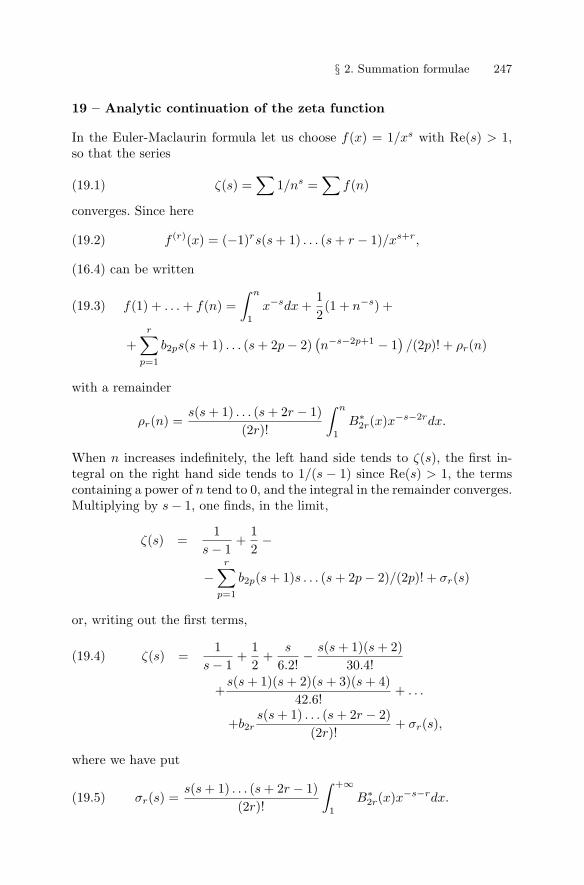
§ 2. Summation formulae 247
19 – Analytic continuation of the zeta function
In the Euler-Maclaurin formula let us choose f(x) = 1/xs with Re(s) > 1,so that the series
ζ(s) =∑
1/ns =∑
f(n)(19.1)
converges. Since here
f (r)(x) = (−1)rs(s + 1) . . . (s + r − 1)/xs+r,(19.2)
(16.4) can be written
f(1) + . . . + f(n) =∫ n
1
x−sdx +12(1 + n−s) +(19.3)
+r∑
p=1
b2ps(s + 1) . . . (s + 2p − 2)(n−s−2p+1 − 1
)/(2p)! + ρr(n)
with a remainder
ρr(n) =s(s + 1) . . . (s + 2r − 1)
(2r)!
∫ n
1
B∗2r(x)x−s−2rdx.
When n increases indefinitely, the left hand side tends to ζ(s), the first in-tegral on the right hand side tends to 1/(s − 1) since Re(s) > 1, the termscontaining a power of n tend to 0, and the integral in the remainder converges.Multiplying by s − 1, one finds, in the limit,
ζ(s) =1
s − 1+
12−
−r∑
p=1
b2p(s + 1)s . . . (s + 2p − 2)/(2p)! + σr(s)
or, writing out the first terms,
ζ(s) =1
s − 1+
12
+s
6.2!− s(s + 1)(s + 2)
30.4!(19.4)
+s(s + 1)(s + 2)(s + 3)(s + 4)
42.6!+ . . .
+b2rs(s + 1) . . . (s + 2r − 2)
(2r)!+ σr(s),
where we have put
σr(s) =s(s + 1) . . . (s + 2r − 1)
(2r)!
∫ +∞
1
B∗2r(x)x−s−rdx.(19.5)
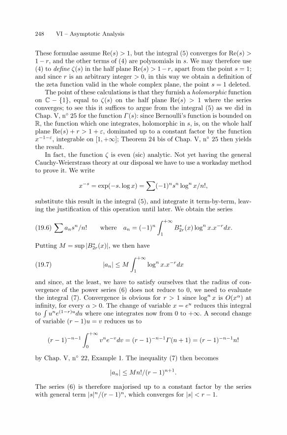
248 VI – Asymptotic Analysis
These formulae assume Re(s) > 1, but the integral (5) converges for Re(s) >1− r, and the other terms of (4) are polynomials in s. We may therefore use(4) to define ζ(s) in the half plane Re(s) > 1− r, apart from the point s = 1;and since r is an arbitrary integer > 0, in this way we obtain a definition ofthe zeta function valid in the whole complex plane, the point s = 1 deleted.
The point of these calculations is that they furnish a holomorphic functionon C − {1}, equal to ζ(s) on the half plane Re(s) > 1 where the seriesconverges; to see this it suffices to argue from the integral (5) as we did inChap. V, n◦ 25 for the function Γ (s): since Bernoulli’s function is bounded onR, the function which one integrates, holomorphic in s, is, on the whole halfplane Re(s) + r > 1 + ε, dominated up to a constant factor by the functionx−1−ε, integrable on [1,+∞]; Theorem 24 bis of Chap. V, n◦ 25 then yieldsthe result.
In fact, the function ζ is even (sic) analytic. Not yet having the generalCauchy-Weierstrass theory at our disposal we have to use a workaday methodto prove it. We write
x−s = exp(−s. log x) =∑
(−1)nsn logn x/n!,
substitute this result in the integral (5), and integrate it term-by-term, leav-ing the justification of this operation until later. We obtain the series
∑ansn/n! where an = (−1)n
∫ +∞
1
B∗2r(x) logn x.x−rdx.(19.6)
Putting M = sup |B∗2r(x)|, we then have
|an| ≤ M
∫ +∞
1
logn x.x−rdx(19.7)
and since, at the least, we have to satisfy ourselves that the radius of con-vergence of the power series (6) does not reduce to 0, we need to evaluatethe integral (7). Convergence is obvious for r > 1 since logn x is O(xα) atinfinity, for every α > 0. The change of variable x = eu reduces this integralto∫
une(1−r)udu where one integrates now from 0 to +∞. A second changeof variable (r − 1)u = v reduces us to
(r − 1)−n−1
∫ +∞
0
vne−vdv = (r − 1)−n−1Γ (n + 1) = (r − 1)−n−1n!
by Chap. V, n◦ 22, Example 1. The inequality (7) then becomes
|an| ≤ Mn!/(r − 1)n+1.
The series (6) is therefore majorised up to a constant factor by the serieswith general term |s|n/(r − 1)n, which converges for |s| < r − 1.
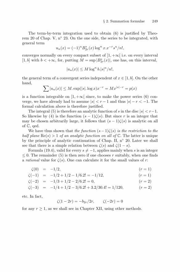
§ 2. Summation formulae 249
The term-by-term integration used to obtain (6) is justified by Theo-rem 20 of Chap. V, n◦ 23. On the one side, the series to be integrated, withgeneral term
un(x) = (−1)nB∗2r(x) logn x.x−rsn/n!,
converges normally on every compact subset of [1,+∞[ i.e. on every interval[1, b] with b < +∞, for, putting M = sup |B∗
2r(x)|, one has, on this interval,
|un(x)| ≤ M logn b.|s|n/n!,
the general term of a convergent series independent of x ∈ [1, b]. On the otherhand, ∑
|un(x)| ≤ M. exp(|s|. log x)x−r = Mx|s|−r = p(x)
is a function integrable on [1,+∞[ since, to make the power series (6) con-verge, we have already had to assume |s| < r − 1 and thus |s| − r < −1. Theformal calculation above is therefore justified.
The integral (5) is therefore an analytic function of s in the disc |s| < r−1.So likewise by (4) is the function (s − 1)ζ(s). But since r is an integer thatmay be chosen arbitrarily large, it follows that (s − 1)ζ(s) is analytic on allof C, qed.
We have thus shown that the function (s− 1)ζ(s) is the restriction to thehalf plane Re(s) > 1 of an analytic function on all of C. The latter is uniqueby the principle of analytic continuation of Chap. II, n◦ 20. Later we shallsee that there is a simple relation between ζ(s) and ζ(1 − s).
Formula (19.4), valid for every s �= −1, applies mainly when s is an integer≤ 0. The remainder (5) is then zero if one chooses r suitably, when one findsa rational value for ζ(s). One can calculate it for the small values of r:
ζ(0) = −1/2, (r = 1)ζ(−1) = −1/2 + 1/2 − 1/6.2! = −1/12, (r = 1)ζ(−2) = −1/3 + 1/2 − 2/6.2! = 0, (r = 2)ζ(−3) = −1/4 + 1/2 − 3/6.2! + 3.2/30.4! = 1/120, (r = 2)
etc. In fact,ζ(1 − 2r) = −b2r/2r, ζ(−2r) = 0
for any r ≥ 1, as we shall see in Chapter XII, using other methods.
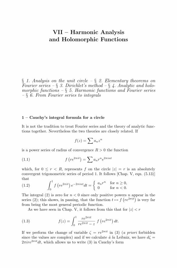
VII – Harmonic Analysisand Holomorphic Functions
§ 1. Analysis on the unit circle – § 2. Elementary theorems onFourier series – § 3. Dirichlet’s method – § 4. Analytic and holo-morphic functions – § 5. Harmonic functions and Fourier series– § 6. From Fourier series to integrals
1 – Cauchy’s integral formula for a circle
It is not the tradition to treat Fourier series and the theory of analytic func-tions together. Nevertheless the two theories are closely related. If
f(z) =∑
anzn
is a power series of radius of convergence R > 0 the function
f(re2πit)
=∑
anrne2πint(1.1)
which, for 0 ≤ r < R, represents f on the circle |z| = r is an absolutelyconvergent trigonometric series of period 1. It follows [Chap. V, eqn. (5.13)]that ∫ 1
0
f(re2πit)e−2πintdt =
{anrn for n ≥ 0,0 for n < 0.
(1.2)
The integral (2) is zero for n < 0 since only positive powers n appear in theseries (2); this shows, in passing, that the function t → f
(re2πit)
is very farfrom being the most general periodic function.
As we have seen in Chap. V, it follows from this that for |z| < r
f(z) =∫ 1
0
re2πit
re2πit − zf(re2πit)dt.(1.3)
If we perform the change of variable ζ = re2πit in (3) (a priori forbiddensince the values are complex) and if we calculate a la Leibniz, we have dζ =2πire2πitdt, which allows us to write (3) in Cauchy’s form
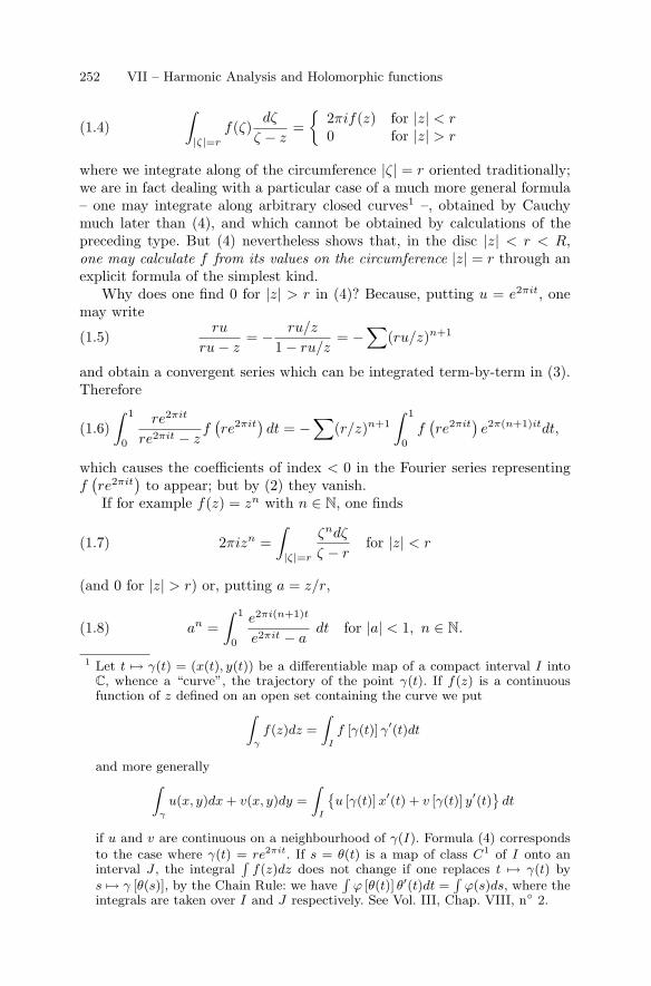
252 VII – Harmonic Analysis and Holomorphic functions
∫|ζ|=r
f(ζ)dζ
ζ − z={
2πif(z) for |z| < r0 for |z| > r
(1.4)
where we integrate along of the circumference |ζ| = r oriented traditionally;we are in fact dealing with a particular case of a much more general formula– one may integrate along arbitrary closed curves1 –, obtained by Cauchymuch later than (4), and which cannot be obtained by calculations of thepreceding type. But (4) nevertheless shows that, in the disc |z| < r < R,one may calculate f from its values on the circumference |z| = r through anexplicit formula of the simplest kind.
Why does one find 0 for |z| > r in (4)? Because, putting u = e2πit, onemay write
ru
ru − z= − ru/z
1 − ru/z= −∑
(ru/z)n+1(1.5)
and obtain a convergent series which can be integrated term-by-term in (3).Therefore∫ 1
0
re2πit
re2πit − zf(re2πit)dt = −
∑(r/z)n+1
∫ 1
0
f(re2πit)e2π(n+1)itdt,(1.6)
which causes the coefficients of index < 0 in the Fourier series representingf(re2πit)
to appear; but by (2) they vanish.If for example f(z) = zn with n ∈ N, one finds
2πizn =∫|ζ|=r
ζndζ
ζ − rfor |z| < r(1.7)
(and 0 for |z| > r) or, putting a = z/r,
an =∫ 1
0
e2πi(n+1)t
e2πit − adt for |a| < 1, n ∈ N.(1.8)
1 Let t �→ γ(t) = (x(t), y(t)) be a differentiable map of a compact interval I intoC, whence a “curve”, the trajectory of the point γ(t). If f(z) is a continuousfunction of z defined on an open set containing the curve we put∫
γ
f(z)dz =
∫I
f [γ(t)] γ′(t)dt
and more generally∫γ
u(x, y)dx + v(x, y)dy =
∫I
{u [γ(t)] x′(t) + v [γ(t)] y′(t)
}dt
if u and v are continuous on a neighbourhood of γ(I). Formula (4) correspondsto the case where γ(t) = re2πit. If s = θ(t) is a map of class C1 of I onto aninterval J , the integral
∫f(z)dz does not change if one replaces t �→ γ(t) by
s �→ γ [θ(s)], by the Chain Rule: we have∫
ϕ [θ(t)] θ′(t)dt =∫
ϕ(s)ds, where theintegrals are taken over I and J respectively. See Vol. III, Chap. VIII, n◦ 2.
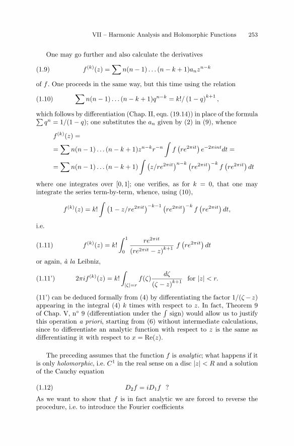
VII – Harmonic Analysis and Holomorphic Functions 253
One may go further and also calculate the derivatives
f (k)(z) =∑
n(n − 1) . . . (n − k + 1)anzn−k(1.9)
of f . One proceeds in the same way, but this time using the relation∑n(n − 1) . . . (n − k + 1)qn−k = k!/ (1 − q)k+1
,(1.10)
which follows by differentiation (Chap. II, eqn. (19.14)) in place of the formula∑qn = 1/(1 − q); one substitutes the an given by (2) in (9), whence
f (k)(z) =
=∑
n(n − 1) . . . (n − k + 1)zn−kr−n
∫f(re2πit)e−2πintdt =
=∑
n(n − 1) . . . (n − k + 1)∫ (
z/re2πit)n−k (
re2πit)−k
f(re2πit)dt
where one integrates over [0, 1]; one verifies, as for k = 0, that one mayintegrate the series term-by-term, whence, using (10),
f (k)(z) = k!∫ (
1 − z/re2πit)−k−1 (
re2πit)−k
f(re2πit)dt,
i.e.
f (k)(z) = k!∫ 1
0
re2πit
(re2πit − z)k+1f(re2πit)dt(1.11)
or again, a la Leibniz,
2πif (k)(z) = k!∫|ζ|=r
f(ζ)dζ
(ζ − z)k+1for |z| < r.(1.11’)
(11’) can be deduced formally from (4) by differentiating the factor 1/(ζ − z)appearing in the integral (4) k times with respect to z. In fact, Theorem 9of Chap. V, n◦ 9 (differentiation under the
∫sign) would allow us to justify
this operation a priori, starting from (6) without intermediate calculations,since to differentiate an analytic function with respect to z is the same asdifferentiating it with respect to x = Re(z).
The preceding assumes that the function f is analytic; what happens if itis only holomorphic, i.e. C1 in the real sense on a disc |z| < R and a solutionof the Cauchy equation
D2f = iD1f ?(1.12)
As we want to show that f is in fact analytic we are forced to reverse theprocedure, i.e. to introduce the Fourier coefficients
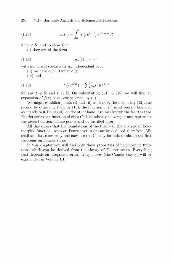
254 VII – Harmonic Analysis and Holomorphic functions
an(r) =∫ 1
0
f(re2πit)e−2πintdt(1.13)
for r < R, and to show that(i) they are of the form
an(r) = anrn(1.14)
with numerical coefficients an independent of r,(ii) we have an = 0 for n < 0,(iii) and
f(re2πit)
=∑
an(r)e2πint(1.15)
for any t ∈ R and r < R. On substituting (14) in (15) we will find anexpansion of f(z) as an entire series, by (ii).
We might establish points (i) and (ii) as of now, the first using (12), thesecond by observing that, by (13), the function an(r) must remain boundedas r tends to 0. Point (iii), on the other hand, assumes known the fact that theFourier series of a function of class C1 is absolutely convergent and representsthe given function. These points will be justified later.
All this shows that the foundations of the theory of the analytic or holo-morphic functions rests on Fourier series or can be deduced therefrom. Weshall see that conversely one may use the Cauchy formula to obtain the firsttheorems on Fourier series.
In this chapter you will find only those properties of holomorphic func-tions which can be derived from the theory of Fourier series. Everythingthat depends on integrals over arbitrary curves (the Cauchy theory) will beexpounded in Volume III.
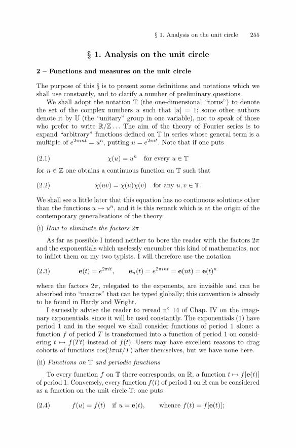
§ 1. Analysis on the unit circle 255
§ 1. Analysis on the unit circle
2 – Functions and measures on the unit circle
The purpose of this § is to present some definitions and notations which weshall use constantly, and to clarify a number of preliminary questions.
We shall adopt the notation T (the one-dimensional “torus”) to denotethe set of the complex numbers u such that |u| = 1; some other authorsdenote it by U (the “unitary” group in one variable), not to speak of thosewho prefer to write R/Z . . . The aim of the theory of Fourier series is toexpand “arbitrary” functions defined on T in series whose general term is amultiple of e2πint = un, putting u = e2πit. Note that if one puts
χ(u) = un for every u ∈ T(2.1)
for n ∈ Z one obtains a continuous function on T such that
χ(uv) = χ(u)χ(v) for any u, v ∈ T.(2.2)
We shall see a little later that this equation has no continuous solutions otherthan the functions u → un, and it is this remark which is at the origin of thecontemporary generalisations of the theory.
(i) How to eliminate the factors 2π
As far as possible I intend neither to bore the reader with the factors 2πand the exponentials which uselessly encumber this kind of mathematics, norto inflict them on my two typists. I will therefore use the notation
e(t) = e2πit, en(t) = e2πint = e(nt) = e(t)n(2.3)
where the factors 2π, relegated to the exponents, are invisible and can beabsorbed into “macros” that can be typed globally; this convention is alreadyto be found in Hardy and Wright.
I earnestly advise the reader to reread n◦ 14 of Chap. IV on the imagi-nary exponentials, since it will be used constantly. The exponentials (1) haveperiod 1 and in the sequel we shall consider functions of period 1 alone: afunction f of period T is transformed into a function of period 1 on consid-ering t → f(Tt) instead of f(t). Users may have excellent reasons to dragcohorts of functions cos(2πnt/T ) after themselves, but we have none here.
(ii) Functions on T and periodic functions
To every function f on T there corresponds, on R, a function t → f [e(t)]of period 1. Conversely, every function f(t) of period 1 on R can be consideredas a function on the unit circle T: one puts
f(u) = f(t) if u = e(t), whence f(t) = f [e(t)];(2.4)
256 VII – Harmonic Analysis and Holomorphic Functions
since f(t + 1) = f(t) there is no ambiguity, t being determined modulo aninteger when one knows u. This is an abuse of notation since a function on Ris not, strictly speaking, a function on T; but it is indispensable to be able toadopt both of these two points of view; and to use different notations for thetwo functions which correspond “canonically” according to (4) would makethe text unreadable.
This correspondence between functions defined on these different setspreserves continuity. Since the map t → e(t) of R on T is continuous, thecontinuity of f at a point of T trivially implies its continuity at the corre-sponding points of R. On the other hand, even though the map t → e(t) isnot globally bijective, it maps every compact interval I ⊂ R of length strictly< 1 bijectively onto a closed arc K ⊂ T of the circle. Restricted to I, themap t → e(t) therefore has an inverse map K → I which is also continuous(Chap. III, n◦ 9). The map t → e(t) thus inversely transforms every contin-uous function on I into a continuous function on K. This is equivalent tosaying that a function defined on the circle |u| = 1 is continuous if and onlyif it is a continuous function of the polar angle, or argument, of the point u,as is obvious from a sketch. § 4 of Chap. IV on the uniform branches of the“function” Arg z also shows that on a neighbourhood of each point u0 ∈ Tor even on T with a point removed, for example on T − {1}, but not on thewhole of T, one may choose t so that it is a continuous function of u = e(t).
(iii) Characterisation of the exponentials
The correspondence (4) allows us to show that the functional equation(2) has no continuous solutions apart from the functions (1). To start with,note that for every continuous solution of (2)
|χ(u)| = 1 for every u ∈ T;
this relates to the fact that, endowed with the usual multiplication and topol-ogy of the complex numbers, T is a “compact group”: since the continuousfunction χ is bounded on the compact set T, it follows that for every u ∈ T,the family of the numbers χ(un) = χ(u)n for n ∈ Z is likewise bounded; itremains then to show that the only complex numbers z such that
supn∈Z
|zn| < +∞
are those of modulus 1, which is clear. Since (2) implies χ(u−1)
= χ(u)−1,it follows that every continuous solution of (2) also satisfies
χ(u−1)
= χ(u)(2.5)
and more generally
χ(uv−1)
= χ(u)χ(v)(2.6)
§ 1. Analysis on the unit circle 257
for any u, v ∈ T.On the other hand, the continuous function χ(x) = χ(e(x)) = χ
(e2πix)
on R satisfies the functional equation
χ(x + y) = χ(x)χ(y)
of Chap. IV, n◦ 13. We have shown there that every solution of the latter isof the form
χ(x) = exp(cx)(2.7)
with a constant c ∈ C, on condition that we know that the function χ has aderivative at the origin.
But, in fact, continuity suffices, and implies much more than differentia-bility at the origin. To see this, one chooses on R a function ϕ ∈ D(R) and,as in Chap. V, n◦ 27, one regularises χ by means of the convolution product
χ � ϕ(x) =∫
R
χ(x − y)ϕ(y)dy =∫
R
χ(x)χ(y)−1ϕ(y)dy = c.χ(x);(2.8)
the constant c =∫
χ(y)−1ϕ(y)dy may be assumed to be nonzero, since, ifχ�ϕ were zero for every ϕ ∈ D(R), then so would be the function χ (Chap. V,n◦ 27, Theorem 26). Now the function χ � ϕ is C∞ for every ϕ ∈ D(R). Solikewise is χ.
We may now apply the result of Chap. IV, n◦ 13 and write (7). Butin the present case |χ(x)| = 1 for every x ∈ R. Putting c = a + ib witha and b real, we have | exp(cx)| = exp(ax) for x ∈ R, whence a = 0 andχ(x) = exp(ibx) with b real. For the result to be of period 1 it is necessaryand sufficient that exp(ib) = 1, i.e. that b = 2πn with an n ∈ Z. Finally wefind χ(x) = exp(2πinx), whence χ(u) = un, qed.
We shall later call every function of the form u → un = χ(u) a char-acter of T. This terminology comes from the theory of commutative groups(Chap. XI), where one considers the solutions of the functional equation (2)systematically on the given group G. If one assumes G commutative andfinite – the simplest case, involving only algebra –, every function on G is,and in a unique way, a linear combination of characters of G, of which thereare Card(G); this is the simplest version of the Fourier transform, thoughdating from very much later than Fourier himself (even though Dirichlethad used this idea for the group Z/nZ in proving his theorem on arithmeticprogressions).
(iv) Mean value of a function on a circle
In the theory of analytic functions one often considers the mean value ofa function over a circle, and, in that of the periodic functions, over a periodinterval. There is no difference between these two ways of integrating.
First, on a circle |z| = r, a function of z, analytic or not, can, as we haveseen, be transformed into a function of period 1 by putting
258 VII – Harmonic Analysis and Holomorphic Functions
z = re(t) = re2πit(2.9)
or into a function of period 2π on putting z = reit. Its mean value aroundthe circle |z| = r is, by definition, the number which we denote by∫
T
f(ru)dm(u) =∫ 1
0
f(re(t))dt =12π
∫ 2π
0
f(reit)dt(2.10)
where T, we recall, denotes the unit circle |u| = 1 in the complex plane. Moregenerally we put
m(f) =∫
T
f(u)dm(u) =∫ 1
0
f(e(t))dt =12π
∫ 2π
0
f(eit)dt(2.11)
for every “reasonable”, for example regulated2, function f on T. We will usethe norms
‖f‖ = ‖f‖T = sup |f(u)|, ‖f‖1 =∫
T
|f(u)|dm(u),
‖f‖2 =(∫
T
|f(u)|2 dm(u))1/2
as in R.We may in fact, in (11), integrate over any interval of length 1, since∫ 1
0
f(t)dt =∫ a+1
a
f(t)dt =∫ a+1
a
f(b + t)dt(2.12)
for any a, b ∈ R for every function f of period 1 on R (Chap. V, end of n◦ 2).Besides, even in the case of arbitrary functions of period T on R, the
formulae only mention the mean values of the functions over a period interval;it is convenient to write, here again,
m(f) =∫ 1
0
f(t)dt =12π
∫ 2π
0
=1T
∫ T
0
=∮
,(2.13)
as we study functions of period 1, 2π or T ; the sign∮
dispenses us fromwriting the limits of integration since, by definition, it denotes the mean2 This means, as one prefers, that the corresponding periodic function is regulated,
i.e. has left and right limit values at every point of R, or that the function givenon T enjoys the same property, the limit values at a point of T being defined inthe obvious way. The BL theorem being valid for the compact set T, it comesto the same to require that for every r > 0 there exists a partition of T into afinite number of arcs of circles, of any kind, on each of which the given functionis constant to within r. One may also define, using such partitions, the notionof step function on T, and, generally, transpose to T the arguments of Chap. V,n◦ 7.
§ 1. Analysis on the unit circle 259
value over a period (or even over several periods) of the integrand. In fact,and without express mention to the contrary, all the integrals in dt will be, inthe rest of this chapter, apart from § 6, extended over any interval of length1.
As we have seen in Chap. V, n◦ 5, which the reader is invited to readagain, the essential formulae in the theory of absolutely convergent Fourierseries (calculation of the coefficients and of the scalar product) stem from the“orthogonality relations” of the exponentials, the relation (5.2) of Chap. V.With the notation just introduced, they can be written∫
ep(u)eq(u)dm(u) ={
1 if p = q,0 if p �= q.
The scalar product (f | g) of two periodic functions introduced in Chap. V,eqn. (5.4), will now be written
(f | g) =∫
f(u)g(u)dm(u) = m(fg).
The orthogonality relations thus signify that if χ and χ′ are two characters ofT, then (χ |χ′) = 1 or 0 according to whether χ and χ′ are equal or different.
(v) Measures on T
The notation dm(u) in (11) indicates that we are integrating with respectto a measure on T. We have defined this notion in Chap. V, n◦ 30 in the caseof a compact set X ⊂ C: one considers the vector space C0(X) of scalarfunctions defined and continuous on X, endowed with the norm
‖f‖X = supx∈X
|f(x)|(2.14)
of uniform convergence on X; a measure on X is then, by definition, a mapµ of C0(X) into C which is linear and continuous, i.e. satisfies an inequality
|µ(f)| ≤ M(µ) ‖f‖X(2.15)
which allows one to pass to the limit under the∫
sign when integrating auniformly convergent sequence of functions fn ∈ C0(X) with respect to µ. Ameasure is said to be positive if µ(f) ≥ 0 for every function f ≥ 0. It is clearthat formula (11) defines such a measure on T.
In the case of the measure m, all that we have said in Chap. V trans-poses immediately to integration on T, starting with the notion of integrablefunction (Chap. V, n◦ 2); it will be the same for an arbitrary measure µ oncewe have defined the integrable functions in this case. The proper theory ofFourier series uses the Lebesgue integral – for m or any other measure onT – and has, historically, constituted one of the principal justifications ormotivations for it. Since we cannot yet do this here, we shall confine our-selves, in this chapter, without exceptions, to considering regulated, mostly
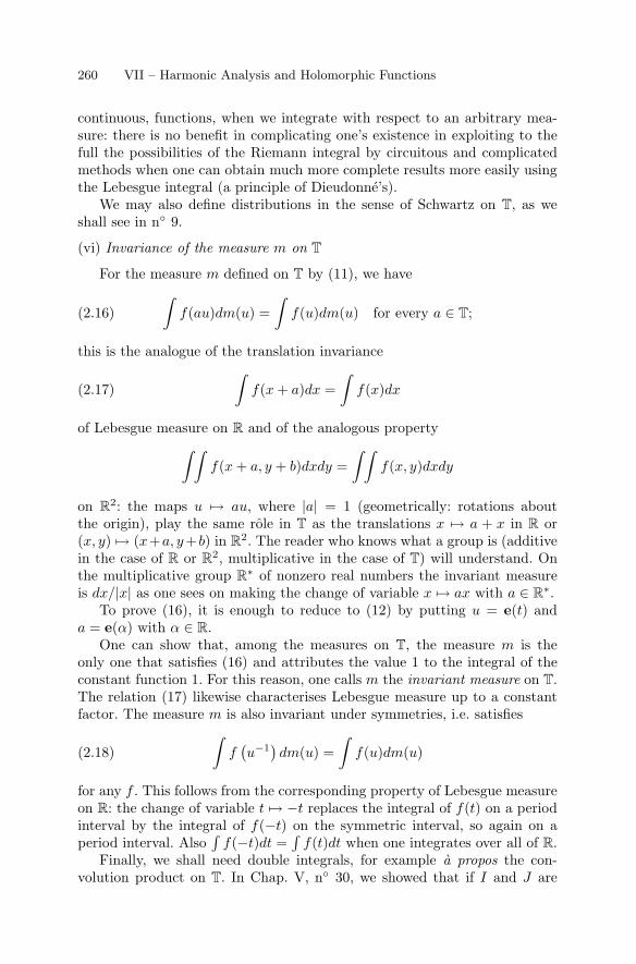
260 VII – Harmonic Analysis and Holomorphic Functions
continuous, functions, when we integrate with respect to an arbitrary mea-sure: there is no benefit in complicating one’s existence in exploiting to thefull the possibilities of the Riemann integral by circuitous and complicatedmethods when one can obtain much more complete results more easily usingthe Lebesgue integral (a principle of Dieudonne’s).
We may also define distributions in the sense of Schwartz on T, as weshall see in n◦ 9.
(vi) Invariance of the measure m on T
For the measure m defined on T by (11), we have∫f(au)dm(u) =
∫f(u)dm(u) for every a ∈ T;(2.16)
this is the analogue of the translation invariance∫f(x + a)dx =
∫f(x)dx(2.17)
of Lebesgue measure on R and of the analogous property∫ ∫f(x + a, y + b)dxdy =
∫ ∫f(x, y)dxdy
on R2: the maps u → au, where |a| = 1 (geometrically: rotations aboutthe origin), play the same role in T as the translations x → a + x in R or(x, y) → (x+a, y+b) in R2. The reader who knows what a group is (additivein the case of R or R2, multiplicative in the case of T) will understand. Onthe multiplicative group R∗ of nonzero real numbers the invariant measureis dx/|x| as one sees on making the change of variable x → ax with a ∈ R∗.
To prove (16), it is enough to reduce to (12) by putting u = e(t) anda = e(α) with α ∈ R.
One can show that, among the measures on T, the measure m is theonly one that satisfies (16) and attributes the value 1 to the integral of theconstant function 1. For this reason, one calls m the invariant measure on T.The relation (17) likewise characterises Lebesgue measure up to a constantfactor. The measure m is also invariant under symmetries, i.e. satisfies∫
f(u−1)dm(u) =
∫f(u)dm(u)(2.18)
for any f . This follows from the corresponding property of Lebesgue measureon R: the change of variable t → −t replaces the integral of f(t) on a periodinterval by the integral of f(−t) on the symmetric interval, so again on aperiod interval. Also
∫f(−t)dt =
∫f(t)dt when one integrates over all of R.
Finally, we shall need double integrals, for example a propos the con-volution product on T. In Chap. V, n◦ 30, we showed that if I and J are
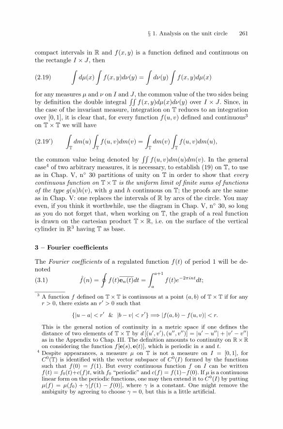
§ 1. Analysis on the unit circle 261
compact intervals in R and f(x, y) is a function defined and continuous onthe rectangle I × J , then∫
dµ(x)∫
f(x, y)dν(y) =∫
dν(y)∫
f(x, y)dµ(x)(2.19)
for any measures µ and ν on I and J , the common value of the two sides beingby definition the double integral
∫∫f(x, y)dµ(x)dν(y) over I × J . Since, in
the case of the invariant measure, integration on T reduces to an integrationover [0, 1], it is clear that, for every function f(u, v) defined and continuous3
on T × T we will have∫T
dm(u)∫
T
f(u, v)dm(v) =∫
T
dm(v)∫
T
f(u, v)dm(u),(2.19’)
the common value being denoted by∫∫
f(u, v)dm(u)dm(v). In the generalcase4 of two arbitrary measures, it is necessary, to establish (19) on T, to useas in Chap. V, n◦ 30 partitions of unity on T in order to show that everycontinuous function on T×T is the uniform limit of finite sums of functionsof the type g(u)h(v), with g and h continuous on T; the proofs are the sameas in Chap. V: one replaces the intervals of R by arcs of the circle. You mayeven, if you think it worthwhile, use the diagram in Chap. V, n◦ 30, so longas you do not forget that, when working on T, the graph of a real functionis drawn on the cartesian product T × R, i.e. on the surface of the verticalcylinder in R3 having T as base.
3 – Fourier coefficients
The Fourier coefficients of a regulated function f(t) of period 1 will be de-noted
f(n) =∮
f(t)en(t)dt =∫ a+1
a
f(t)e−2πintdt;(3.1)
3 A function f defined on T × T is continuous at a point (a, b) of T × T if for anyr > 0, there exists an r′ > 0 such that
{|u − a| < r′ & |b − v| < r′} =⇒ |f(a, b) − f(u, v)| < r.
This is the general notion of continuity in a metric space if one defines thedistance of two elements of T × T by d [(u′, v′), (u′′, v′′)] = |u′ − u′′| + |v′ − v′′|as in the Appendix to Chap. III. The definition amounts to continuity on R×Ron considering the function f [e(s), e(t)], which is periodic in s and t.
4 Despite appearances, a measure µ on T is not a measure on I = [0, 1], forC0(T) is identified with the vector subspace of C0(I) formed by the functionssuch that f(0) = f(1). But every continuous function f on I can be writtenf(t) = f0(t)+c(f)t, with f0 “periodic” and c(f) = f(1)−f(0). If µ is a continuouslinear form on the periodic functions, one may then extend it to C0(I) by puttingµ(f) = µ(f0) + γ[f(1) − f(0)], where γ is a constant. One might remove theambiguity by agreeing to choose γ = 0, but this is a little artificial.
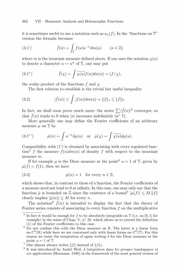
262 VII – Harmonic Analysis and Holomorphic Functions
it is sometimes useful to use a notation such as an(f). In the “functions on T”version the formula becomes
f(n) =∫
T
f(u)u−ndm(u) (n ∈ Z)(3.1’)
where m is the invariant measure defined above. If one uses the notation χ(u)to denote a character u → un of T, one may put
f(χ) =∫
χ(u)f(u)dm(u) = (f |χ),(3.1”)
the scalar product of the functions f and χ.The first relation to establish is the trivial but useful inequality
|f(n)| ≤∫
|f(u)|dm(u) = ‖f‖1 ≤ ‖f‖T.(3.2)
In fact, we shall soon prove much more: the series∑ |f(n)|2 converges, so
that f(n) tends to 0 when |n| increases indefinitely (n◦ 7).More generally one may define the Fourier coefficients of an arbitrary
measure µ on T by
µ(n) =∫
u−ndµ(u) or µ(χ) =∫
χ(u)dµ(u).(3.1”’)
Compatibility with (1’) is obtained by associating with every regulated func-tion5 f the measure f(u)dm(u) of density f with respect to the invariantmeasure m.
If for example µ is the Dirac measure at the point6 u = 1 of T, given byµ(f) = f(1), then we have
µ(n) = 1 for every n ∈ Z,(3.3)
which shows that, in contrast to those of a function, the Fourier coefficients ofa measure need not tend to 0 at infinity. In this case, one may only say that thefunction µ is bounded on Z since the existence of a bound7 |µ(f)| ≤ M.‖f‖clearly implies |µ(n)| ≤ M for every n.
The notation8 f(n) is intended to display the fact that the theory ofFourier series consists of associating to every function f on the multiplicative5 In fact it would be enough for f to be absolutely integrable on T (i.e. on [0, 1] for
example) in the sense of Chap. V, n◦ 22, which allows us to extend the definition(1) of the Fourier coefficients to this case.
6 Do not confuse this with the Dirac measure on R. The latter is a linear formon C0(R) while here we are concerned only with linear forms on C0(T). For thisreason we resist the temptation of again writing δ for the Dirac measure at thepoint u = 1 of T.
7 One almost always writes ‖f‖ instead of ‖f‖T.8 It was introduced by Andre Weil, L’integration dans les groupes topologiques et
ses applications (Hermann, 1940) in the framework of the most general version of
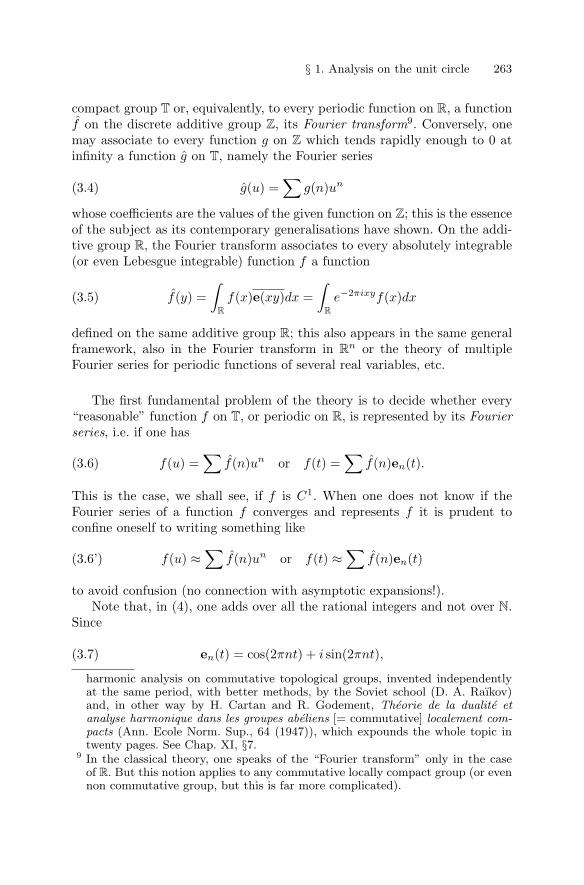
§ 1. Analysis on the unit circle 263
compact group T or, equivalently, to every periodic function on R, a functionf on the discrete additive group Z, its Fourier transform9. Conversely, onemay associate to every function g on Z which tends rapidly enough to 0 atinfinity a function g on T, namely the Fourier series
g(u) =∑
g(n)un(3.4)
whose coefficients are the values of the given function on Z; this is the essenceof the subject as its contemporary generalisations have shown. On the addi-tive group R, the Fourier transform associates to every absolutely integrable(or even Lebesgue integrable) function f a function
f(y) =∫
R
f(x)e(xy)dx =∫
R
e−2πixyf(x)dx(3.5)
defined on the same additive group R; this also appears in the same generalframework, also in the Fourier transform in Rn or the theory of multipleFourier series for periodic functions of several real variables, etc.
The first fundamental problem of the theory is to decide whether every“reasonable” function f on T, or periodic on R, is represented by its Fourierseries, i.e. if one has
f(u) =∑
f(n)un or f(t) =∑
f(n)en(t).(3.6)
This is the case, we shall see, if f is C1. When one does not know if theFourier series of a function f converges and represents f it is prudent toconfine oneself to writing something like
f(u) ≈∑
f(n)un or f(t) ≈∑
f(n)en(t)(3.6’)
to avoid confusion (no connection with asymptotic expansions!).Note that, in (4), one adds over all the rational integers and not over N.
Since
en(t) = cos(2πnt) + i sin(2πnt),(3.7)
harmonic analysis on commutative topological groups, invented independentlyat the same period, with better methods, by the Soviet school (D. A. Raıkov)and, in other way by H. Cartan and R. Godement, Theorie de la dualite etanalyse harmonique dans les groupes abeliens [= commutative] localement com-pacts (Ann. Ecole Norm. Sup., 64 (1947)), which expounds the whole topic intwenty pages. See Chap. XI, §7.
9 In the classical theory, one speaks of the “Fourier transform” only in the caseof R. But this notion applies to any commutative locally compact group (or evennon commutative group, but this is far more complicated).
264 VII – Harmonic Analysis and Holomorphic Functions
the series (4) can always be put in the traditional trigonometric form
a0 +∞∑1
bn cos(2πnt) + cn sin(2πnt)(3.8)
(take the terms with indices n and −n together), or, if the bn and cn are real,∑In cos[2πn(t − ωn)]
with “phase lags” ωn and “intensities” In ≥ 0 for n > 0, but using this formcomplicates the calculations; the formulae
en(x + y) = en(x)en(y), en(t) = en(t)−1 = e−n(t),(3.9)ep(t)eq(t) = ep+q(t)
are simpler than the analogous trigonometric formulae and lend themselvesto the generalisations to group theory10.
As we have already said elsewhere, one has always to observe that theseries (4) being extended over Z and not over N, it has a meaning only if itconverges unconditionally, i.e. if∑∣∣∣f(n)
∣∣∣ < +∞.(3.10)
This is the case for the functions f ∈ C1(T) as we shall see in n◦ 8, but (10)is very likely to be false when one attempts to study more general functions.In this case, one gives a sense to the series by putting, by definition,
∑Z
f(n)en(t) = limN→+∞
N∑−N
f(n)en(t) = lim fN (t),(3.11)
which considerably increases the chances of convergence and amounts, infact, to considering the traditional series (8) and its usual partial sums fN (t).
10 If G is a commutative group endowed with a locally compact topology, one callsa character of G any continuous map χ : G −→ T such that χ(uv) = χ(u)χ(v).It is clear that if χ′ and χ′′ are two characters, then so likewise is the productfunction χ(u) = χ′(u)χ′′(u); endowed with this multiplication, the set of thecharacters of G becomes a group; on endowing this with the topology of compactconvergence one obtains a new commutative locally compact group, the “dual”
G of G. Since there always exists a positive measure dm(u) on G invariant
under the translations u �→ uv, one may associate a “Fourier transform” f(χ) =∫χ(u)f(u)dm(u) to every function f on G decreasing rapidly enough at infinity.
One may then choose a positive invariant measure dm(χ) on G so that conversely
f(u) =∫
χ(u)f(χ)dm(χ) under reasonable hypotheses on f . In the case where
G = T, the characters are the en(t), whence G = Z, and the last formula (9)
shows that the “multiplication” on G is precisely the addition on Z.
§ 1. Analysis on the unit circle 265
These are trigonometric polynomials since only a finite number of nonzerocoefficients feature in fN . If one knew that for every continuous function fon T, the fN converged uniformly on T to f , one would obtain Weierstrass’approximation theorem of Chap. V, n◦ 28 for periodic functions. Unfortu-nately not, even if one demands only simple convergence; to obtain uniformconvergence when f is continuous it is enough to substitute for the fN theirarithmetic means (f1 + . . . + fN )/N as we shall see (Fejer’s theorem), whichwill provide a proof – there are others – of the approximation theorem.
In a general way, and as we have already said elsewhere, we have to warnthe reader to exercise the most extreme prudence once he steps outside theframework of the C1 functions: most of the statements that one might believeobvious are false and, when they are correct, they are never obvious. This isone of the charms of the theory for those whom it attracts, and the reasonwhy it played such large role in the development of analysis during all theXIXth century and a large part of the following one: when one does notunderstand one tries to understand, and this often brings one much furtherthan one had imagined. One of the first traps of the theory is to believe thatif a trigonometric series
a0 +∑
bn cos 2πnt + cn sin 2πnt,
with arbitrarily given coefficients converges for any t, than it must be theFourier series of its sum. False: though a simple limit of continuous functionsand so “measurable” in the sense of Lebesgue, the sum of the series can failto be integrable. The first theorems proved by Cantor in 1870 say that, for atrigonometric series,
(i) the coefficients bn and cn tend to 0 if the general term bn cos(2πnt) +cn sin(2πnt) tends to 0 at every point of an interval I of nonzero length,and therefore if the series converges on I,
(ii) if the series converges to 0 for every t ∈ R, then all the coefficients arezero (“obvious”, but try to prove it . . .).
It was in trying to weaken the hypothesis of the statement (ii), i.e. in tryingto characterise the sets E ⊂ [0, 1] such that
f(t) = 0 for every t ∈ E =⇒ an = bn = 0
(“sets of uniqueness”), that Cantor was led to construct more and morebaroque sets in R, then to his theory of transfinite numbers. Do not confusethis, as we have already said, with the naıve trivialities of Chap. I, whichwould not have led him to the edge of sanity if he had not been already pre-disposed. This kind of question continues to be the object of much research11;most mathematicians and a fortiori users are happy with much less subtleresults of universal use.11 See for example J-P. Kahane and R. Salem, Ensembles parfaits and series
trigonometriques (Paris, Hermann, nouvelle ed. 1987) and J.-P. Kahane and P.G. Lemarie-Rieusset, Series de Fourier et ondelettes (Paris, Cassini, 1997).
266 VII – Harmonic Analysis and Holomorphic Functions
4 – Convolution product on T
The invariance of the measure m under translation leads to useful formulae.For example, the left hand side of formula (2.19’) does not change if in it onereplaces f(u, v) by f(u, av) for an a ∈ T independent of v; in particular, onecan, for each u, replace v by uv, or u−1v, since u is a variable independentof v, whence the formulae∫ ∫
f(u, v)dm(u)dm(v) =∫ ∫
f(u, u−1v
)dm(u)dm(v),(∗) ∫ ∫
f(u, v)dm(u)dm(v) =∫ ∫
f(uv, v−1
)dm(u)dm(v) :(∗∗)
one integrates first with respect to u, makes the change of variable u → uv−1,then integrates with respect to v, finally one replaces v by v−1. Similar resultin R: if f(x, y) is, for simplicity, continuous and of compact support in R2,then ∫ ∫
f(x, y)dxdy =∫ ∫
f(x + y,−y)dxdy
for ∫ ∫f(x, y)dxdy =
=∫
dy
∫f(x, y)dx =
∫dy
∫f(x − y, y)dx (using x −→ x − y)
=∫
dx
∫f(x − y, y)dy =
∫dx
∫f(x + y,−y)dy (using y −→ −y)
=∫ ∫
f(x + y,−y)dxdy.
The invariant measure allows us, as in R (Chap. V, n◦ 27), to define theconvolution product12
f � g(u) =∫
f(uv−1)g(v)dm(v) =
∫f(w)g(uw−1)dm(w) = g � f(u)(4.1)
of two regulated functions on T or, in the “periodic functions on R” version,
f � g(t) =∮
f(t − s)g(s)ds =∮
g(t − s)f(s)ds,(4.1’)
integrating over a period. The equality of the two integrals in (1) is obtainedby means of the change of variable v → uv−1 = w (or s → t − s), thecomposition of a translation v → uv followed by a symmetry v −→ v−1;12 A symbol such as f g(u) denotes the value at the point u of the function f g
and replaces the expression (f g)(u).
§ 1. Analysis on the unit circle 267
see (∗). A convenient way to simplify the theoretical calculations on Fourierseries is to remark that if χ is a character of T, the convolution product
f � χ(u) =∫
χ(uv−1)f(v)dm(v) =(4.2)
= χ(u)∫
χ(v)f(v)dm(v) = f(χ)χ(u)
is the general term of the Fourier series of f . The relation (3.6) can then,when it is true, be written
f(t) =∑
f � en(t) or f(u) =∑
f � χ(u)(4.3)
where, in the second case, one sums over all the characters of T. Symbolically,one may also write it as f =
∑f � en =
∑f � χ, which has the advantage
of not presupposing the mode of convergence that one chooses: simple con-vergence, uniform convergence, convergence in mean, etc. It is precisely thechoice of the mode of convergence to make (3) correct that is the whole theoryof Fourier series; (3) is always correct in the sense of distributions as we shallsee, but the convergence of a sequence or series of distributions is, in prac-tice, the weakest invented from Newton to nowadays. (Paradoxically, this is infact the interest of distributions: everything which converges in a reasonablesense, or does not converge, converges in the sense of distributions).
The convolution product has properties similar to those13 obtained inChap. II, n◦ 18, Example 3, for functions defined on Z: but the proofs areless easy. We shall restrict ourselves to functions which are regulated and sobounded; going further requires recourse to the Lebesgue integral and willbe expounded in Chap. XI, n◦ 25 in the general framework of group theory– for this is a matter of group theory as the case of the convolution producton Z has already shown.
First of all the inequality |f(uv−1)g(v)| ≤ ‖f‖ |g(v)|, valid for all u and v,shows that, always,
‖f � g‖ ≤ ‖f‖ ‖g‖1 ≤ ‖f‖ ‖g‖ ·
We shall deduce from this that the function f � g is continuous. If f is con-tinuous this follows directly from Chap. V, n◦ 9 (Theorem 9, (i)) since weare integrating the continuous function f(uv−1) with respect to the measureg(v)dm(v). In the general case there exists a sequence (fn) of continuousfunctions (see the lemma in n◦ 8 below) such that lim ‖f − fn‖1 = 0; then,by (4),
‖f � g − fn � g‖ ≤ ‖g‖ ‖f − fn‖1 ,
13 apart from the existence of a unit element: this would be a function e(u) suchthat one had
∫f(uv−1)e(v)dv = f(u) for any f ; the only candidate is the Dirac
“function”, which is a measure and not a function.
268 VII – Harmonic Analysis and Holomorphic Functions
from which f ∗g is the uniform limit of the continuous functions fn�g, whencethe result.
Now let us establish the relations
f � (g + h) = f � g + f � h, (f � g) � h = f � (g � h)(4.5)
for f , g and h regulated. The first is obvious. To obtain the associativityformula let us first consider an integral of the form∫ ∫
ϕ(uv)f(u)g(v)dm(u)dm(v)(4.6)
where ϕ is continuous and f and g are regulated. Theorem 10 of Chap. V,n◦ 9, and the invariance of the measure show that it is equal to∫
g(v)dm(v)∫
ϕ(uv)f(u)dm(u)
=∫
g(v)dm(v)∫
ϕ(z)f(zv−1)dm(z)
=∫
ϕ(z)dm(z)∫
f(zv−1)g(v)dm(v);
whence the relation∫ ∫ϕ(uv)f(u)g(v)dm(u)dm(v) =
∫ϕ(z).f � g(z)dm(z).(4.7)
This done, let us consider the triple integral
I(ϕ) =∫ ∫ ∫
ϕ(uvw)f(u)g(v)h(w)dm(u)dm(v)dm(w)(4.8)
where f , g and h are regulated. Theorem 10 of Chap. V, n◦ 9, which is clearlyvalid for multiple integrals, shows us that on the one hand
I(ϕ) =∫
h(w)dm(w)∫ ∫
ϕ(uvw)f(u)g(v)dm(u)dm(v)
=∫
h(w)dm(w)∫
ϕ(xw)f � g(x)dm(x) by (7)
=∫ ∫
ϕ(xw) · f � g(x) · h(w)dm(x)dm(w)
=∫
ϕ(z).(f � g) � h(z)dm(z)
applying (7) again, to the functions f � g and h.
But one can also calculate I(ϕ) alternatively as
§ 1. Analysis on the unit circle 269
I(ϕ) =∫
f(u)dm(u)∫ ∫
ϕ(uvw)g(v)h(w)dm(v)dm(w)
=∫
f(u)dm(u)∫
ϕ(ux).g � h(x)dm(x) by (7)
=∫ ∫
ϕ(ux)f(u)g � h(x)dm(u)dm(x)
=∫
ϕ(z).f � (g � h)(z)dm(z)
by applying (7) now to f and g � h. Comparing these results we see that thefunction F = f � (g � h)− (f � g) � h satisfies
∫ϕ(z)F (z)dm(z) = 0 for every
continuous ϕ on T. Now F is itself continuous. One may therefore choose ϕto be the conjugate of F , whence
∫ |F (z)|2dm(z) = 0 and F = 0 (Chap. V,n◦ 7, Theorem 7), which proves associativity for regulated functions, if notyet for all the integrable functions of the Appendix to Chap. V.
Along with (4) for the uniform norm, we also have
‖f � g‖1 ≤ ‖f‖1.‖g‖1.(4.9)
Replacing f and g by their absolute values does not change the right handside, but increases the left hand side, since
|f � g(u)| ≤∫
|f(uv−1)|.|g(v)|dm(v) = |f | � |g|(u);
so it is enough to prove (8) for positive f and g. Relation (7) with ϕ = 1shows that
‖f � g‖1 = ‖f‖1 ‖g‖1
in this case, qed.The Fourier series of a convolution product is calculated very simply from
the formula
f � g(n) = f(n)g(n).(4.10)
To see this, use the associativity of the convolution product:
f � g(n)en = (f � g) � en = f � (g � en) =
= f � (g(n)en) = g(n)f � en = g(n)f(n)en.
For the inverse Fourier transform, which starts from a function f(n) in L1(Z),i.e. such that
∑ |f(n)| < +∞, and leads to a function
f(u) =∑
f(n)un,(4.11)
one has likewise, for the convolution product on Z (Chap. II, n◦ 18, Exam-ple 3),
270 VII – Harmonic Analysis and Holomorphic Functions
f � g(u) =∑
f � g(n)un =∑
f(p)g(n − p)un =∑
f(p)g(q)up+q =
=∑
f(p)g(q)upuq =∑
f(p)up∑
g(q)uq = f(u)g(u).
The Fourier transform thus interchanges convolution products and ordinaryproducts.
This last result is particularly obvious in the framework of measures. Letµ and ν be two measures on T and let us calculates the product
µ(χ)ν(χ) =∫
χ(u)dµ(u)∫
χ(v)dν(v) =(4.12)
=∫ ∫
χ(u)χ(v)dµ(u)dν(v) =
=∫ ∫
χ(uv)dµ(u)dν(v)
of their Fourier transforms. This leads us to consider more generally the map
λ : f −→∫ ∫
f(uv)dµ(u)dν(v)(4.13)
of C0(T) into C; this is clearly a linear form on C0(T), and it is continuous:
|λ(f)| ≤∣∣∣∣∫
dµ(v)∣∣∣ ∫ f(uv)dν(u)
∣∣∣∣∣∣∣ ≤ M(µ)M(ν)‖f‖.
Consequently, λ is again a measure which one calls the convolution productof the measures µ and ν, notation λ = µ � ν. Clearly λ is positive if µ and νare. With these conventions the formula (12) can be written
µ(χ)ν(χ) = λ(χ) where λ = µ � ν.(4.14)
One finds (4) again on considering the measures dµ(u) = f(u)dm(u) anddν(u) = g(u)dm(u), as the reader can easily verify.
There is no simple formula analogous to (1) for defining or calculatingthe convolution product of two measures; the simplicity of the definition (13)shows once more the advantage in defining measures as linear forms on thecontinuous functions and not starting from a function of sets.
5 – Dirac sequences in T
As in R, the convolution product is linked to Dirac sequences on T, formedby regulated functions ϕn(u) such that
f(1) = lim∫
f(u)ϕn(u)dm(u)(5.1)
for every regulated function f continuous at the point u = 1.
§ 1. Analysis on the unit circle 271
The conditions to impose on them are the same as in Chap. V, n◦ 27.The first is that ∫
ϕn(u)dm(u) = 1 for every n;(D 1)
and then f(1) =∫
f(1)ϕn(u)dm(u), whence∣∣∣∣∫
f(u)ϕn(u)dm(u) − f(1)∣∣∣∣ ≤∫
|f(u) − f(1)|.|ϕn(u)|dm(u).(5.2)
Let us take an r > 0, and, on the right hand side of (2), distinguish thecontributions of the arcs |u−1| < δ and |u−1| > δ of T for some δ > 0 yet tobe decided. Since f is continuous at the origin, one can, for r given, chooseδ so that
|u − 1| < δ =⇒ |f(u) − f(1)| < r.(5.3)
If one assumes that
sup∫
|ϕn(u)| dm(u) = M < +∞,(D 2)
the contribution of this “small” arc to the total integral is ≤ Mr. On the“large” arc |u − 1| > δ we have |f(u) − f(1)| ≤ 2‖f‖ since f is bounded;the corresponding integral is thus, up to a factor 2‖f‖, bounded by that of|ϕn(u)|. Assume now that, for any r and δ, there exists an integer N(δ, r)such that
n > N(δ, r) =⇒∫|u−1|>δ
|ϕn(u)| dm(u) < r,
in other words that
limn→∞
∫|u−1|>δ
|ϕn(u)| dm(u) = 0 for every δ > 0.(D 3)
The preceding arguments now show that for every r and every δ satisfying(3) we will have∫
|f(u) − f(1)|. |ϕn(u)| dm(u) ≤ (M + 2‖f‖)r(5.4)
for every n > N(δ, r), whence (1).The conditions (D 1), (D 2) and (D 3) may therefore be taken as the
definition of the Dirac sequences on T.The most frequent case is that where the ϕn are all positive; (D 1) then
implies (D 2) with M = 1. To achieve (D 3) it is simplest to assume that forevery δ > 0 the functions ϕn converge uniformly to 0 on the arc |u − 1| ≥ δof T, in other words that
limϕn(u) = 0 uniformly on every compact K ⊂ T − {1}(5.5)
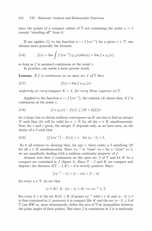
272 VII – Harmonic Analysis and Holomorphic Functions
since the points of a compact subset of T not containing the point u = 1remain “standing off” from it.
If one applies (1) to the function u → f(vu−1)
for a given v ∈ T, oneobtains more generally the formula
f(v) = lim∫
f(vu−1)ϕn(u)dm(u) = lim f � ϕn(v),(5.6)
so long as f is assumed continuous at the point v.In practice, one needs a more precise result.
Lemma. If f is continuous on an open arc J of T then
f(v) = lim f � ϕn(v)(5.7)
uniformly on every compact K ⊂ J , for every Dirac sequence on T.
Applied to the function u → f(vu−1), the relation (4) shows that, if f is
continuous at the point v,
|f � ϕn(v) − f(v)| ≤ (M + 2‖f‖)r(5.8)
for n large; but to obtain uniform convergence on K one has to find an integerN such that (8) will be valid for n > N for all the v ∈ K simultaneously.Now, for r and v given, the integer N depends only, as we have seen, on thechoice of a δ such that∣∣f (vu−1
)− f(v)∣∣ < r for |u − 1| < δ.(5.9)
So it all reduces to showing that, for any r, there exists a δ satisfying (9)for all v ∈ K simultaneously. Since vu−1 is “close” to v for u “close” to 1,we are manifestly dealing with a uniform continuity property of f .
Assume now that f continuous on the open arc J of T and let K be acompact arc contained in J (figure 1). Since T − J and K are compact anddisjoint, the distance d(T − J, K) = d is strictly positive. Since∣∣vu−1 − v
∣∣ = |v − vu| = |1 − u|
for every u ∈ T, we see that
(v ∈ K) & (|u − 1| < d) =⇒ vu−1 ∈ J.
For every δ < d, the set K(δ) ⊃ K of points vu−1 with v ∈ K and |u−1| ≤ δis thus contained in J ; moreover it is compact like K and the arc |u−1| ≤ δ ofT (use BW or, more elementarily, define the arcs of T by inequalities betweenthe polar angles of their points). But since f is continuous in J it is uniformly
§ 1. Analysis on the unit circle 273
Fig. 1.
continuous on K(δ). So we see that for any given r > 0 there exists a δ > 0such that (8) holds for all v ∈ K, qed.
We leave to the reader the task of verifying, as in Chap. V, n◦ 27, that ifthe ϕn are indefinitely differentiable, then so likewise are the functions f �ϕn.This follows in the usual way from the standard theorem on differentiationunder the
∫sign (Chap. V, n◦ 9).
274 VII – Harmonic Analysis and Holomorphic Functions
§ 2. Elementary theorems on Fourier series
6 – Absolutely convergent Fourier series
Almost all the simultaneously simple and important results in the theory ofFourier series, especially those which can be generalised, can be deduced fromone fundamental statement:
Theorem 1 (Weierstrass). Every continuous periodic function is the uni-form limit of trigonometric polynomials.
Instead of proving this now, we shall, in this §, show how one may use it;we shall present an “elementary” proof later (n◦ 12, Theorem 8 and n◦ 23),more complicated than the general “abstract” Stone-Weierstrass theorem ofChap. V, n◦ 28.
The most immediate consequence of Theorem 1 is the following:
Theorem 2. If f is a continuous function on T such that∑ |f(n)| < +∞,
thenf(u) =
∑f(n)un for every u ∈ T.
Let us denote the right hand side by g(u). This is the sum of an absolutelyconvergent Fourier series, whence (Chap. V, n◦ 5) g(n) = f(n) for every n.Putting f = g + h, we see that all the Fourier coefficients of the function hvanish.
The relation h(n) = 0 for every n means that, with respect to the standardscalar product
(f | g) =∫
f(u)g(u)dm(u)
of two functions on T, the function h is “orthogonal” to all the charactersu → un of T : (h |χ) = 0. It is therefore also orthogonal to every linearcombination of a finite number of these functions, i.e. to every trigonometricpolynomial p.
Now h is continuous like f (by hypothesis) and g (the sum of a normallyconvergent series of continuous functions). By Theorem 1, there thereforeexists a sequence (pn) of trigonometric polynomials which converges to huniformly on T. Since the functions h(u)pn(u) convergent to |h(u)|2 uniformlyon T we deduce that∫
|h(u)|2dm(u) = lim∫
h(u)pn(u)dm(u) = lim(h | pn) = 0.
The function |h(u)|2 being continuous and positive, we have h = 0 (Chap. V,n◦ 2), whence f = g, qed.
Here is an easy consequence of Theorem 2: for a continuous function fto be represented by an absolutely convergent Fourier series, it is necessary
§ 2. Elementary theorems on Fourier series 275
and sufficient that∑ |f(n)| < +∞. The condition is sufficient by Theorem 2.
We know on the other hand (Chap. V, n◦ 5) that if a function f , necessarilycontinuous, is the sum of an absolutely convergent Fourier series, then thecoefficients of the latter must be the numbers f(n); the one and only serieswhich represents f is then the Fourier series of f .
The theorem of Cantor mentioned above shows much more: two distincttrigonometric series (i.e. not having the same coefficients) and everywhereconvergent (absolutely or not) cannot have the same sum.
7 – Hilbertian calculations
Let us denote by H the complex vector space (of infinite dimension) of reg-ulated functions on T and let us endow it with the usual scalar product
(f | g) =∫
f(u)g(u)dm(u).(7.1)
It has the same properties as in Chap. V, n◦ 3: it is a linear function of f forg given, we also have
(g, f) = (f | g)(7.2)
and finally
(f | f) =∫
|f(u)|2dm(u) ≥ 0(7.3)
for any f . As in Chap. V and, more generally, as in every pre-Hilbert space(Appendix to Chap. III), it therefore satisfies the Cauchy-Schwarz inequality
|(f | g)|2 ≤ (f | f)(g | g).(7.4)
We deduce that the expression
‖f‖2 = (f | f)1/2 =(∫
|f(u)|2dm(u))1/2
(7.5)
has the properties
‖λf‖2 = |λ|.‖f‖2, ‖f + g‖2 ≤ ‖f‖2 + ‖g‖2,(7.6)
of a “norm” on the vector space H of regulated functions on T, except that therelation ‖f‖2 = 0 shows only that the set {f(u) �= 0} is countable (Chap. V,n◦ 7, Theorem 7) and not that f = 0. This is not important since tworegulated functions which are equal outside a countable set have the sameintegrals and so the same Fourier series.
As in the case of the norm of uniform convergence, the second relation(6) shows that the expression
276 VII – Harmonic Analysis and Holomorphic Functions
d2(f, g) = ‖f − g‖2 =(∫
|f(u) − g(u)|2 dm(u))1/2
is a “distance” between f and g (distance in quadratic mean).This done, one says that two functions f and g are orthogonal if (f | g) = 0,
a concept we have already used above. We now have the Pythagoras relation
‖f + g‖22 = ‖f‖2
2 + ‖g‖22(7.7)
since (f +g | f +g) = (f | f)+(f | g)+(g | f)+(g | g). This extends to a finitesum of pairwise orthogonal functions fi: indeed(∑
fi |∑
fi
)=∑
(fi | fj) =∑
(fi | fi) if (fi | fj) = 0 for i �= j.
In particular, (ep | eq) = 0 or 1, whence(∑apep |∑
bqeq
)=∑
apbp(7.8)
at least when dealing with finite sums, i.e. trigonometric polynomials.With these definitions, the Fourier coefficients of a function f are, as
we have already seen, given by f(n) = (f | en) where en is the exponentialfunction en(t), in version R, or un, in version T. If we consider the partialsum
fN =∑
|n|≤N
f(n)en(7.9)
of the Fourier series of f , we have (fN | en) = f(n) = (f | en) for |n| ≤ Nby (8), and so (f − fN | en) = 0. The function f − fN being orthogonal tothe exponentials en such that |n| ≤ N it is also orthogonal to every linearcombination of the these, and in particular to the function fN itself. Sincef = (f − fN ) + fN , Pythagoras’ theorem shows that
(f | f) = (fN | fN ) + (f − fN | f − fN ) ≥ (fN | fN ).(7.10)
But by (8)
(fN | fN ) =∑
|n|≤N
∣∣∣f(n)∣∣∣2 .(7.11)
The partial sums of the series with positive terms∑∣∣∣f(n)
∣∣∣2 are thereforebounded above by (f | f); they consequently converge, and we have
∑∣∣∣f(n)∣∣∣2 ≤ (f | f) =
∫|f(u)|2dm(u) =
∮|f(t)|2dt(7.12)
for every regulated function on T.
§ 2. Elementary theorems on Fourier series 277
These calculations, which generalise the traditional ones in R3 startingfrom the “unit vectors” of a system of rectangular coordinates, are validin every pre-Hilbert space. If for example you have a sequence of contin-uous functions Pn(t) on a compact interval I ⊂ R – these are often, inpractice, polynomials or the solutions of differential equations – satisfying∫
Pk(t)Ph(t)dt = 0 or 1 according to whether k �= h or k = h, and if for everycontinuous function f in I you put
cn(f) =∫
I
f(t)Pn(t)dt,(7.13)
then you obtain the inequality∑ |cn(f)|2 ≤ ∫ |f(t)|2dt. In the good cases,
one hopes – while there is life there is hope – to obtain not only an equalitybut even an expansion
f(t) =∑
cn(f)Pn(t)(7.14)
in a convergent series. The Fourier series were, historically, the first case topresent themselves, and have, of course, inspired the many later generalisa-tions of which we have just described the simplest.
8 – The Parseval-Bessel equality
The inequality (7.12) is in reality an equality as we have seen in Chap. V, n◦ 5in the simple case of absolutely convergent Fourier series. We shall now provethis for every regulated function, using Weierstrass’ approximation theorem.
By (7.10) and (7.11), it reduces to proving that ‖f − fN‖2 tends to 0, i.e.that
limN→∞
∫ 1
0
∣∣∣f(t) −∑
|n|≤N
f(n)en(t)∣∣∣2dt = 0,(8.1)
but to write integrals of this kind explicitly would be the best method of notunderstanding the proof, and to avail oneself of Knuth’s software in vain.
In the complex vector space H of the preceding n◦, let HN be the set oftrigonometric polynomials involving only the en, |n| ≤ N , in other words, thevector subspace generated by these 2N + 1 functions; it contains fN . Sincef − fN is orthogonal to the en ∈ HN , it is orthogonal to every p ∈ HN aswe saw above. On writing f − p = (f − fN ) + (fN − p) and observing thatfN − p ∈ HN we then have
(f − p | f − p) = (f − fN | f − fN ) + (fN − p | fN − p)(8.2)≥ (f − fN | f − fN )
for any p ∈ HN . In other words, fN is the point of the vector subspace HN
lying at the minimum distance from f , which is plausible (figure 2) since itthe “orthogonal projection” of f onto HN .
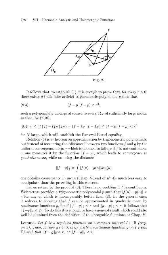
278 VII – Harmonic Analysis and Holomorphic Functions
Fig. 2.
It follows that, to establish (1), it is enough to prove that, for every r > 0,there exists a (indefinite article) trigonometric polynomial p such that
(f − p | f − p) < r2;(8.3)
such a polynomial p belongs of course to every HN of sufficiently large index,so that, by (7.10),
0 ≤ (f | f) − (fN | fN ) = (f − fN | f − fN ) ≤ (f − p | f − p) < r2(8.4)
for N large, which will establish the Parseval-Bessel equality.Relation (3) is a theorem on approximation by trigonometric polynomials;
but instead of measuring the “distance” between two functions f and g by theuniform convergence norm – which is doomed to failure if f is not continuous–, one measures it by the function ‖f − g‖2 which leads to convergence inquadratic mean, while on using the distance
‖f − g‖1 =∫
|f(u) − g(u)|dm(u)
one obtains convergence in mean (Chap. V, end of n◦ 4), much less easy tomanipulate than the preceding in this context.
Let us return to the proof of (3). There is no problem if f is continuous:Weierstrass provides a trigonometric polynomial p such that |f(u)− p(u)| <r for any u, which is incomparably better than (3). In the general case,it reduces to showing that f can be approximated in quadratic mean bycontinuous functions g, for if ‖f − g‖2 < r and ‖g − p‖2 < r, it follows that‖f−p‖2 < 2r. To do this it is enough to have a general result which could alsowell be obtained from the definition of the integrable functions at Chap. V:
Lemma. Let f be a regulated function on a compact interval I ⊂ R (resp.on T). Then, for every r > 0, there exists a continuous function g on I (resp.T) such that ‖f − g‖2 < r, or ‖f − g‖1 < r.
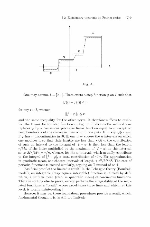
§ 2. Elementary theorems on Fourier series 279
Fig. 3.
One may assume I = [0, 1]. There exists a step function ϕ on I such that
|f(t) − ϕ(t)| ≤ r
for any t ∈ I, whence‖f − ϕ‖1 ≤ r
and the same inequality for the other norm. It therefore suffices to estab-lish the lemma for the step function ϕ. Figure 3 indicates the method: onereplaces ϕ by a continuous piecewise linear function equal to ϕ except onneighbourhoods of the discontinuities of ϕ; if one puts M = sup |ϕ(t)| andif ϕ has n discontinuities in [0, 1], one may choose the n intervals on whichone modifies it so that their lengths are less than r/Mn; the contributionof such an interval to the integral of |f − ϕ| is then less than the lengthr/Mn of the latter multiplied by the maximum of |f − ϕ| on this interval,so to Mr/Mn = r/n, whence, for the n intervals which actually contributeto the integral of |f − ϕ|, a total contribution of ≤ r. For approximationin quadratic mean, one chooses intervals of length < r2/M2n2. The case ofperiodic functions is treated similarly, arguing on T instead of on I.
[Artificial proof of too limited a result. In the Lebesgue theory (Bourbakimodel), an integrable (resp. square integrable) function is, almost by defi-nition, a limit in mean (resp. in quadratic mean) of continuous functions.There is nothing else to prove, except perhaps the integrability of the regu-lated functions, a “result” whose proof takes three lines and which, at thislevel, is totally uninteresting.]
However it may be, these roundabout procedures provide a result, which,fundamental though it is, is still too limited:
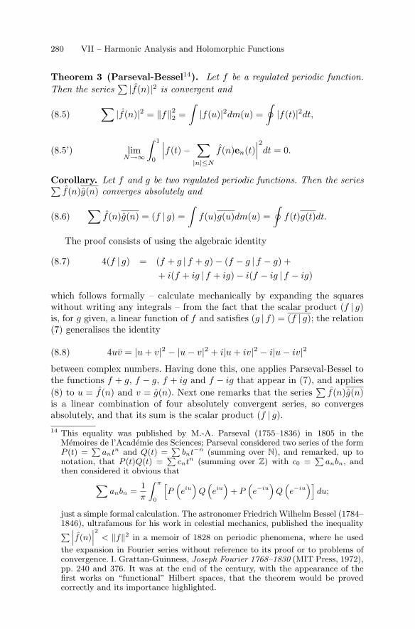
280 VII – Harmonic Analysis and Holomorphic Functions
Theorem 3 (Parseval-Bessel14). Let f be a regulated periodic function.Then the series
∑ |f(n)|2 is convergent and
∑|f(n)|2 = ‖f‖2
2 =∫
|f(u)|2dm(u) =∮
|f(t)|2dt,(8.5)
limN→∞
∫ 1
0
∣∣∣f(t) −∑
|n|≤N
f(n)en(t)∣∣∣2dt = 0.(8.5’)
Corollary. Let f and g be two regulated periodic functions. Then the series∑f(n)g(n) converges absolutely and
∑f(n)g(n) = (f | g) =
∫f(u)g(u)dm(u) =
∮f(t)g(t)dt.(8.6)
The proof consists of using the algebraic identity
4(f | g) = (f + g | f + g) − (f − g | f − g) +(8.7)+ i(f + ig | f + ig) − i(f − ig | f − ig)
which follows formally – calculate mechanically by expanding the squareswithout writing any integrals – from the fact that the scalar product (f | g)is, for g given, a linear function of f and satisfies (g | f) = (f | g); the relation(7) generalises the identity
4uv = |u + v|2 − |u − v|2 + i|u + iv|2 − i|u − iv|2(8.8)
between complex numbers. Having done this, one applies Parseval-Bessel tothe functions f + g, f − g, f + ig and f − ig that appear in (7), and applies(8) to u = f(n) and v = g(n). Next one remarks that the series
∑f(n)g(n)
is a linear combination of four absolutely convergent series, so convergesabsolutely, and that its sum is the scalar product (f | g).14 This equality was published by M.-A. Parseval (1755–1836) in 1805 in the
Memoires de l’Academie des Sciences; Parseval considered two series of the formP (t) =
∑antn and Q(t) =
∑bnt−n (summing over N), and remarked, up to
notation, that P (t)Q(t) =∑
cntn (summing over Z) with c0 =∑
anbn, andthen considered it obvious that∑
anbn =1
π
∫ π
0
[P(eiu)
Q(eiu)
+ P(e−iu)
Q(e−iu)]
du;
just a simple formal calculation. The astronomer Friedrich Wilhelm Bessel (1784–1846), ultrafamous for his work in celestial mechanics, published the inequality∑∣∣∣f(n)
∣∣∣2 < ‖f‖2 in a memoir of 1828 on periodic phenomena, where he used
the expansion in Fourier series without reference to its proof or to problems ofconvergence. I. Grattan-Guinness, Joseph Fourier 1768–1830 (MIT Press, 1972),pp. 240 and 376. It was at the end of the century, with the appearance of thefirst works on “functional” Hilbert spaces, that the theorem would be provedcorrectly and its importance highlighted.
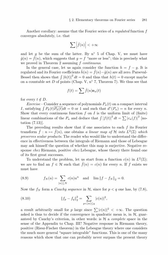
§ 2. Elementary theorems on Fourier series 281
Another corollary: assume that the Fourier series of a regulated function fconverges absolutely, i.e. that∑∣∣∣f(n)
∣∣∣ < +∞
and let g be the sum of the latter. By n◦ 5 of Chap. V, we must haveg(n) = f(n), which suggests that g = f “more or less”; this is precisely whatwe proved in Theorem 2 assuming f continuous.
In the general case, let us again consider the function h = f − g. It isregulated and its Fourier coefficients h(n) = f(n)−g(n) are all zero. Parseval-Bessel then shows that
∫ |h(t)|2 dt = 0 and thus that h(t) = 0 except maybeon a countable set D of points (Chap. V, n◦ 7, Theorem 7). We thus see that
f(t) =∑
f(n)en(t)
for every t /∈ D.Exercise – Consider a sequence of polynomials Pn(t) on a compact interval
I, satisfying∫
Pk(t)Ph(t)dt = 0 or 1 and such that d◦(Pn) = n for every n.Show that every continuous function f on I is the uniform limit of (finite)linear combinations of the Pn and deduce that
∫ |f(t)|2 dt =∑ |cn(f)|2 [no-
tation (7.13)].The preceding results show that if one associates to each f its Fourier
transform f : n → f(n), one obtains a linear map of H into L2(Z) whichpreserves scalar products. The reader who would like to understand the differ-ence in effectiveness between the integrals of Riemann and those of Lebesguemay ask himself the question of whether this map is surjective. Negative re-sponse chez Riemann, positive chez Lebesgue, whose theory there found oneof its first great successes.
To understand the problem, let us start from a function c(n) in L2(Z);we are to find an f ∈ H such that f(n) = c(n) for every n. If f exists wemust have
fN (u) =∑
|n|≤N
c(n)un and lim ‖f − fN‖2 = 0.(8.9)
Now the fN form a Cauchy sequence in H, since for p < q one has, by (7.8),
‖fp − fq‖22 =∑
p<|n|≤q
|c(n)|2,(8.10)
a result arbitrarily small for p large since∑ |c(n)|2 < +∞. The question
asked is thus to decide if the convergence in quadratic mean is, in H, guar-anteed by Cauchy’s criterion, in other words: is H a complete space in thesense of the Appendix to Chap. III? Negative response in Riemann theory,positive (Riesz-Fischer theorem) in the Lebesgue theory where one considersthe much more general “square integrable” functions. This is one of the manyreasons which show that one can probably never surpass the present theory
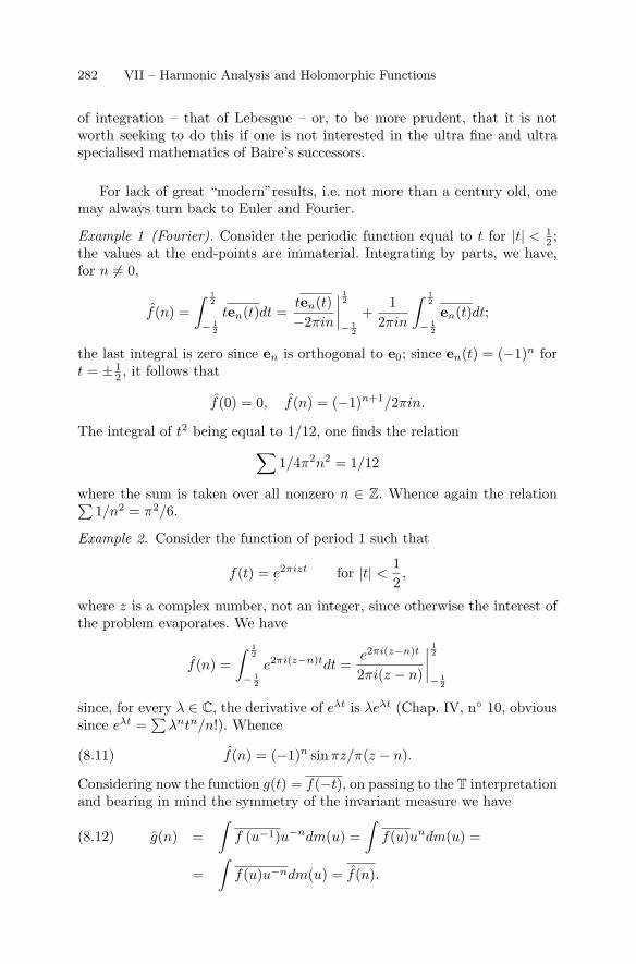
282 VII – Harmonic Analysis and Holomorphic Functions
of integration – that of Lebesgue – or, to be more prudent, that it is notworth seeking to do this if one is not interested in the ultra fine and ultraspecialised mathematics of Baire’s successors.
For lack of great “modern”results, i.e. not more than a century old, onemay always turn back to Euler and Fourier.
Example 1 (Fourier). Consider the periodic function equal to t for |t| < 12 ;
the values at the end-points are immaterial. Integrating by parts, we have,for n �= 0,
f(n) =∫ 1
2
− 12
ten(t)dt =ten(t)−2πin
∣∣∣∣12
− 12
+1
2πin
∫ 12
− 12
en(t)dt;
the last integral is zero since en is orthogonal to e0; since en(t) = (−1)n fort = ± 1
2 , it follows that
f(0) = 0, f(n) = (−1)n+1/2πin.
The integral of t2 being equal to 1/12, one finds the relation∑1/4π2n2 = 1/12
where the sum is taken over all nonzero n ∈ Z. Whence again the relation∑1/n2 = π2/6.
Example 2. Consider the function of period 1 such that
f(t) = e2πizt for |t| <12,
where z is a complex number, not an integer, since otherwise the interest ofthe problem evaporates. We have
f(n) =∫ 1
2
− 12
e2πi(z−n)tdt =e2πi(z−n)t
2πi(z − n)
∣∣∣∣12
− 12
since, for every λ ∈ C, the derivative of eλt is λeλt (Chap. IV, n◦ 10, obvioussince eλt =
∑λntn/n!). Whence
f(n) = (−1)n sin πz/π(z − n).(8.11)
Considering now the function g(t) = f(−t), on passing to the T interpretationand bearing in mind the symmetry of the invariant measure we have
g(n) =∫
f (u−1)u−ndm(u) =∫
f(u)undm(u) =(8.12)
=∫
f(u)u−ndm(u) = f(n).
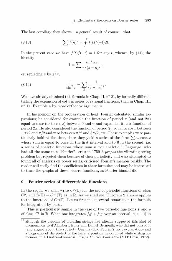
§ 2. Elementary theorems on Fourier series 283
The last corollary then shows – a general result of course – that
∑f(n)2 =
∮f(t)f(−t)dt.(8.13)
In the present case we have f(t)f(−t) = 1 for any t, whence, by (11), theidentity
1 =∑ sin2 πz
π2(z − n)2,
or, replacing z by z/π,
1sin2 z
=∑
Z
1(z − nπ)2
.(8.14)
We have already obtained this formula in Chap. II, n◦ 21, by formally differen-tiating the expansion of cot z in series of rational fractions, then in Chap. III,n◦ 17, Example 4 by more orthodox arguments .
In his memoir on the propagation of heat, Fourier calculated similar ex-pansions; he considered for example the function of period π (and not 2π)equal to sin x (or to cos x) between 0 and π and expanded it as a function ofperiod 2π. He also considered the function of period 2π equal to cos x between−π/2 and π/2 and zero between π/2 and 3π/2, etc. These examples were par-ticularly bold at the time, since they yield a series of the form
∑an cos nx
whose sum is equal to cos x in the first interval and to 0 in the second, i.e.a series of analytic functions whose sum is not analytic15; Lagrange, whohad all the same met “Fourier” series in 1759 a propos the vibrating stringproblem but rejected them because of their periodicity and who attempted tofound all of analysis on power series, criticised Fourier’s memoir briskly. Thereader will easily find the coefficients in these formulae and may be interestedto trace the graphs of these bizarre functions, as Fourier himself did.
9 – Fourier series of differentiable functions
In the sequel we shall write Cp(T) for the set of periodic functions of classCp; and D(T) = C∞(T) as in R. As we shall see, Theorem 2 always appliesto the functions of C1(T). Let us first make several remarks on the formulafor integration by parts.
This is particularly simple in the case of two periodic functions f and gof class C1 in R. When one integrates fg′ + f ′g over an interval [a, a + 1] in
15 although the problem of vibrating strings had already suggested this kind ofphenomenon to d’Alembert, Euler and Daniel Bernoulli, who did not pursue it(and argued about this subject). One may find Fourier’s text, explanations anda biography of the prefect of the Isere, a position he occupied while writing hismemoir, in I. Grattan-Guinness, Joseph Fourier 1768–1830 (MIT Press, 1972).
284 VII – Harmonic Analysis and Holomorphic Functions
R, the term f(a + 1)g(a + 1)− f(a)g(a) cancels to zero because f and g areperiodic. Writing generally f ′(u) for the function which, on T, correspondsthrough f ′(e(t)) = f ′(t) to the periodic function16 f ′(t) on R, we then have∫
f ′(u)g(u)dm(u) = −∫
f(u)g′(u)dm(u)(9.1)
or, in the R version, ∮f ′(t)g(t)dt = −
∮f(t)g′(t)dt.(9.2)
This result extends to the periodic functions which are primitives of regu-lated functions, but this requires some explanations. Periodic or not, a func-tion f is, on R, a primitive of a regulated function f ′ if (i) f is continuous,(ii) f admits right and left derivatives at each point t ∈ R, equal to thelimits f ′(t+) and f ′(t−) of f ′; the derivative f ′ is thus periodic if f is. The-orem 12 bis of Chap. V, n◦ 13, i.e. the FT, being valid for the primitives ofregulated functions, one has
f(1) − f(0) =∮
f ′(t)dt,
so that the mean value of f ′ is zero if f is periodic. Formula (2) remainsvalid since, if f and g are periodic primitives of regulated functions f ′ andg′, necessarily periodic, the function fg is manifestly a periodic primitive off ′g + fg′; since fg is periodic, the integral of f ′g + fg′ over a period is zeroas we have just seen, whence (2).
One must not believe that a regulated periodic function f always admits aperiodic primitive. If indeed – the only possibility up to an additive constant– one puts
F (t) =∫ t
0
f(x)dx
as in Chap. V, n◦ 13, it is clear that F is periodic if and only if the meanvalue of f is zero: write that F (1) = F (0). One could adopt the precedingformula for t ∈ [0, 1[ and define F on R by periodicity, but then one wouldhave
F (1−) − F (1+) = F (1−) − F (0+) = lim[F (1 − ε) − F (ε)] =∫ 1
0
f(t)dt,
whence a discontinuity for t = 1 and more generally for t ∈ Z; not be-ing continuous, F cannot be a primitive of f . In a case of this kind, onehas to add to the right hand side of (2.20’) a term equal to the difference
16 We have f ′(u) = 2πi. lim[f(uv) − f(u)]/(v − 1) as v ∈ T tends to 1.
§ 2. Elementary theorems on Fourier series 285
f(1−)g(1−) − f(0+)g(0+); a notorious source of errors17 in calculation . . .
This done, let us consider a function f ∈ C1(T) and write Df = f ′ forits derivative, a periodic continuous function. An integration by parts thenshows, by (2), that∫ 1
0
Df(t)e−2πintdt = 2πin
∫ 1
0
f(t)e−2πintdt
i.e.
Df(n) = 2πinf(n).(9.3)
This calculation is again valid if f is a periodic primitive of a regulatedperiodic function, as we have seen above. It does not apply to Example 1 ofthe preceding n◦, for the periodic function equal to t on [− 1
2 , 12 [, not being
everywhere continuous, is not a primitive on R.Now we know that the series
∑∣∣Df(n)∣∣2 converges since Df is regulated;
so likewise is the series∑
1/n2. The series∑∣∣Df(n)/n
∣∣ is therefore ab-solutely convergent (Cauchy-Schwarz inequality for series). But Df(n)/n =f(n) up to a constant factor. Consequently:
Theorem 4. Let f be a periodic continuous function, the primitive of aregulated function on R (for example, a periodic function of class C1 on R);then the Fourier series of f is absolutely convergent and
f(t) =∑
f(n)en(t)
for any t ∈ R.
If f is of class C2 one may iterate (3) and obtain
D2f(n) = (2πin)2 f(n),
and so on.The Parseval-Bessel inequality now shows that
∑∣∣∣npf(n)∣∣∣2 < +∞(9.4)
if f ∈ Cp(T), and a fortiori17 Pay attention to the fact that the f ∈ Cp(T) must be of class Cp on R and
not only on a period interval such as [0, 1], since this last property is compatiblewith the existence of discontinuities at 0 and 1 of the derivatives of the periodicfunction considered. For a function f of class Cp on [0, 1] to be extendable to a
periodic function of class Cp on R it is necessary and sufficient that f (k)(0) =
f (k)(1) for every k ≤ p.
286 VII – Harmonic Analysis and Holomorphic Functions
f(n) = o(1/np).(9.5)
One may wonder whether, conversely, these properties characterise theFourier coefficients of functions of class Cp; the answer is negative: for p = 1,the relation (4) is satisfied by every primitive of a regulated function, whichallows many discontinuities in the derivative. But it is worth looking closer.
First, (3) shows that if f is a periodic primitive of a regulated functionDf , then the Fourier series∑
Df(n)en(t) ≈∑
2πinf(n)en(t)(9.6)
of Df is obtained as if one may differentiate that of f term-by-term, eventhough the general theorem on term-by-term differentiation (Chap. III, n◦ 17,Theorem 19 and Example 2) does not necessarily apply here: the discontinu-ities of Df can prevent its Fourier series from converging uniformly or evensimply (whence the ≈ sign).
If, however, the right hand side of (6) converges absolutely for a givenregulated periodic function f , i.e. if
∑ |nf(n)| < +∞, a more restrictivecondition than f(n) = o(1/n), then a fortiori
∑ |f(n)| < +∞; one maythen, as we have seen in n◦ 8, assume that
f(t) =∑
f(n)en(t)
everywhere by modifying f on a countable set; since the derived series con-verges uniformly, we conclude that f is differentiable and that Df(t) =∑
2πinf(n)en(t) is a continuous function: the function f is thus of class C1.More generally, if the Fourier coefficients of a function f satisfy
∑ |npf(n)| <+∞, the function is of class Cp: iterate the argument.
The case where p = ∞, i.e. of the functions f ∈ D(T), is simpler. If f isC∞, in which case (5) applies for any p to the Fourier coefficients of all thesuccessive derivatives of f , one may differentiate the Fourier series of f term-by-term ad libitum and obtain series which are all normally convergent andrepresent the successive derivatives of f ; note that, except for that of f , theyhave no constant term. If, conversely, one takes coefficients c(n) satisfying(5) for any p and if one puts f(t) =
∑c(n)en(t), an absolutely convergent
series and so the Fourier series of f , it is clear that the products nrc(n) againsatisfy (5) for any r and that the series obtained on differentiating the series∑
c(n)en(t) formally r times will converge normally; the standard theoremon term-by-term differentiation (Chap. III, n◦ 17, Theorem 19) then appliesto the series
∑c(n)en(t): f is a C∞ function of which c(n) are the Fourier
coefficients. In conclusion:
Theorem 5. Let c(n) be a scalar function on Z. For there to be a functionf ∈ C∞(T) such that f(n) = c(n) for every n it is necessary and sufficientthat c(n) = O(1/np) for every p ∈ N. One may then differentiate the Fourierseries of f term-by-term any number of times.
A function c on Z satisfying (5) for every p is said to be of rapid decrease.
§ 2. Elementary theorems on Fourier series 287
10 – Distributions on T
The identification of the functions on T with the functions of period 1 on Rhas allowed us to define the spaces Cp(T) in an obvious way for every p ∈ N,and also D(T) = C∞(T). As on the Schwartz space D(R) (Chap. V, n◦ 34)one may define the norms
‖ϕ‖(k) = ‖ϕ‖ + ‖Dϕ‖ + . . . + ‖Dkϕ‖(10.1)
on D(T), and the distances
dk(ϕ,ψ) = ‖ϕ − ψ‖(k),(10.1’)
where ‖ϕ‖ = sup |ϕ(u)| denotes the norm of uniform convergence on T (or,in terms of periodic functions, on R) and where the Drϕ = ϕ(r) are thesuccessive derivatives, again periodic, of the function ϕ. A concept of conver-gence is associated with these norms: a sequence ϕn ∈ D(T) converges to aϕ ∈ D(T) if lim dk(ϕ,ϕn) = 0 for every k, in other words, if for every k > 0one has lim Dkϕn = Dkϕ uniformly on T. This is the mode of convergencewhich allows us to differentiate the given sequence term-by-term ad libitum,to calculate the derivatives of the limit.
This said, a distribution on T is, as on R, a linear map T : D(T) → Cwhich is continuous in the following sense: there exist a k ∈ N and a constantM ≥ 0 such that
|T (ϕ)| ≤ M. ‖ϕ‖(k) for every ϕ ∈ D(T),(10.2)
i.e. |T (ϕ) − T (ψ)| ≤ M. ‖ϕ − ψ‖(k). The smallest integer possible k is calledthe order of T . Then lim T (ϕn) = T (ϕ) if the ϕn ∈ D(T) converge uniformlyto a ϕ ∈ D(T) as do all their successive derivatives of order ≤ k: the othersare not involved.
The examples given in Chap. V, n◦ 34 in the case of R transpose easily tohere, so long as one does not try to integrate the periodic functions on all of R,an integral of this kind clearly being divergent. In particular, every integrablefunction f on T defines a distribution Tf : ϕ → ∫ ϕ(u)f(u)dm(u), and everymeasure µ on T a distribution Tµ : ϕ → ∫ ϕ(u)dµ(u). These distributions areof order 0. A distribution such as ϕ → ∫ ϕ(r)(u)f(u)dm(u) is of order r; weshall see later that up to an additive constant18, every distribution on T isof this type.
It would be convenient to use the Leibniz notation T (ϕ) =∫
ϕ(u)dT (u)for distributions; the definition of the derivative
T ′(ϕ) = −T (ϕ′)(10.3)
18 A constant c is also the constant function u �→ c, so is also a distribution, namelyϕ �→ c∫
ϕ(u)dm(u) = c.m(ϕ).
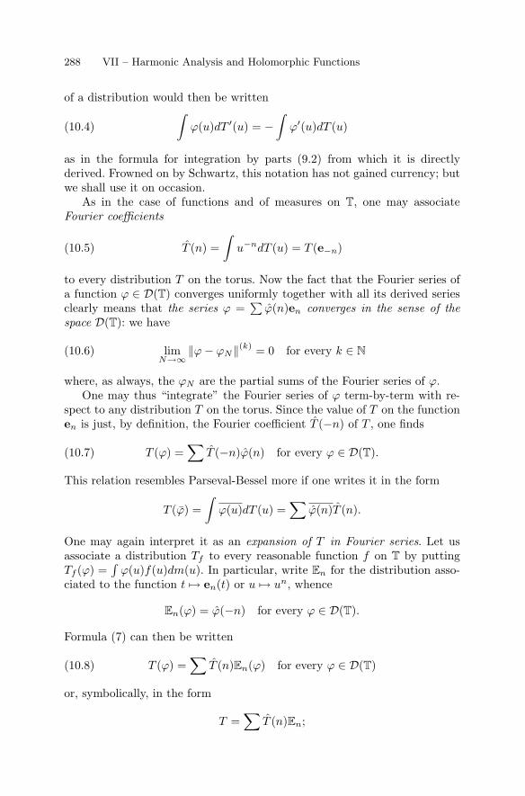
288 VII – Harmonic Analysis and Holomorphic Functions
of a distribution would then be written∫ϕ(u)dT ′(u) = −
∫ϕ′(u)dT (u)(10.4)
as in the formula for integration by parts (9.2) from which it is directlyderived. Frowned on by Schwartz, this notation has not gained currency; butwe shall use it on occasion.
As in the case of functions and of measures on T, one may associateFourier coefficients
T (n) =∫
u−ndT (u) = T (e−n)(10.5)
to every distribution T on the torus. Now the fact that the Fourier series ofa function ϕ ∈ D(T) converges uniformly together with all its derived seriesclearly means that the series ϕ =
∑ϕ(n)en converges in the sense of the
space D(T): we have
limN→∞
‖ϕ − ϕN‖(k) = 0 for every k ∈ N(10.6)
where, as always, the ϕN are the partial sums of the Fourier series of ϕ.One may thus “integrate” the Fourier series of ϕ term-by-term with re-
spect to any distribution T on the torus. Since the value of T on the functionen is just, by definition, the Fourier coefficient T (−n) of T , one finds
T (ϕ) =∑
T (−n)ϕ(n) for every ϕ ∈ D(T).(10.7)
This relation resembles Parseval-Bessel more if one writes it in the form
T (ϕ) =∫
ϕ(u)dT (u) =∑
ϕ(n)T (n).
One may again interpret it as an expansion of T in Fourier series. Let usassociate a distribution Tf to every reasonable function f on T by puttingTf (ϕ) =
∫ϕ(u)f(u)dm(u). In particular, write En for the distribution asso-
ciated to the function t → en(t) or u → un, whence
En(ϕ) = ϕ(−n) for every ϕ ∈ D(T).
Formula (7) can then be written
T (ϕ) =∑
T (n)En(ϕ) for every ϕ ∈ D(T)(10.8)
or, symbolically, in the form
T =∑
T (n)En;
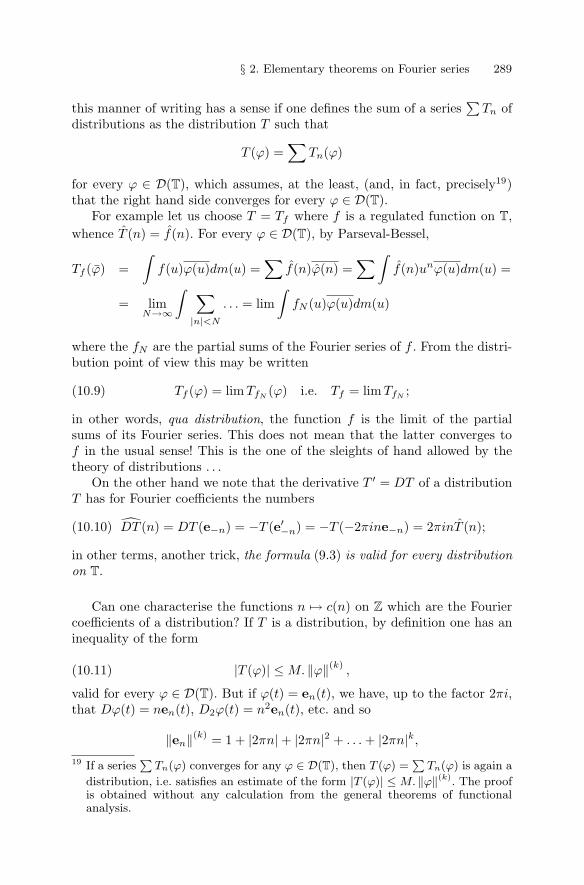
§ 2. Elementary theorems on Fourier series 289
this manner of writing has a sense if one defines the sum of a series∑
Tn ofdistributions as the distribution T such that
T (ϕ) =∑
Tn(ϕ)
for every ϕ ∈ D(T), which assumes, at the least, (and, in fact, precisely19)that the right hand side converges for every ϕ ∈ D(T).
For example let us choose T = Tf where f is a regulated function on T,whence T (n) = f(n). For every ϕ ∈ D(T), by Parseval-Bessel,
Tf (ϕ) =∫
f(u)ϕ(u)dm(u) =∑
f(n)ϕ(n) =∑∫
f(n)unϕ(u)dm(u) =
= limN→∞
∫ ∑|n|<N
. . . = lim∫
fN (u)ϕ(u)dm(u)
where the fN are the partial sums of the Fourier series of f . From the distri-bution point of view this may be written
Tf (ϕ) = limTfN(ϕ) i.e. Tf = limTfN
;(10.9)
in other words, qua distribution, the function f is the limit of the partialsums of its Fourier series. This does not mean that the latter converges tof in the usual sense! This is the one of the sleights of hand allowed by thetheory of distributions . . .
On the other hand we note that the derivative T ′ = DT of a distributionT has for Fourier coefficients the numbers
DT (n) = DT (e−n) = −T (e′−n) = −T (−2πine−n) = 2πinT (n);(10.10)
in other terms, another trick, the formula (9.3) is valid for every distributionon T.
Can one characterise the functions n → c(n) on Z which are the Fouriercoefficients of a distribution? If T is a distribution, by definition one has aninequality of the form
|T (ϕ)| ≤ M. ‖ϕ‖(k),(10.11)
valid for every ϕ ∈ D(T). But if ϕ(t) = en(t), we have, up to the factor 2πi,that Dϕ(t) = nen(t), D2ϕ(t) = n2en(t), etc. and so
‖en‖(k) = 1 + |2πn| + |2πn|2 + . . . + |2πn|k,
19 If a series∑
Tn(ϕ) converges for any ϕ ∈ D(T), then T (ϕ) =∑
Tn(ϕ) is again a
distribution, i.e. satisfies an estimate of the form |T (ϕ)| ≤ M. ‖ϕ‖(k). The proofis obtained without any calculation from the general theorems of functionalanalysis.
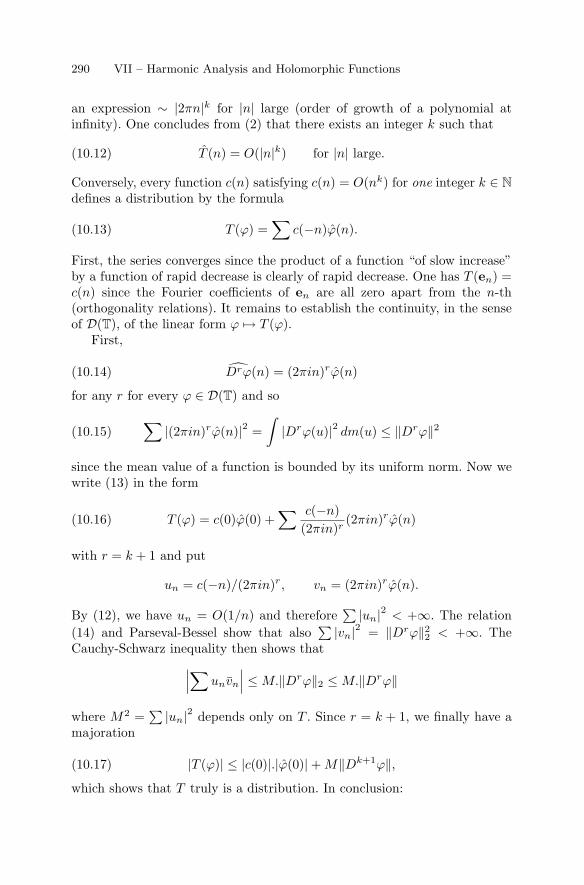
290 VII – Harmonic Analysis and Holomorphic Functions
an expression ∼ |2πn|k for |n| large (order of growth of a polynomial atinfinity). One concludes from (2) that there exists an integer k such that
T (n) = O(|n|k) for |n| large.(10.12)
Conversely, every function c(n) satisfying c(n) = O(nk) for one integer k ∈ Ndefines a distribution by the formula
T (ϕ) =∑
c(−n)ϕ(n).(10.13)
First, the series converges since the product of a function “of slow increase”by a function of rapid decrease is clearly of rapid decrease. One has T (en) =c(n) since the Fourier coefficients of en are all zero apart from the n-th(orthogonality relations). It remains to establish the continuity, in the senseof D(T), of the linear form ϕ → T (ϕ).
First,
Drϕ(n) = (2πin)rϕ(n)(10.14)
for any r for every ϕ ∈ D(T) and so
∑|(2πin)rϕ(n)|2 =
∫|Drϕ(u)|2 dm(u) ≤ ‖Drϕ‖2(10.15)
since the mean value of a function is bounded by its uniform norm. Now wewrite (13) in the form
T (ϕ) = c(0)ϕ(0) +∑ c(−n)
(2πin)r(2πin)rϕ(n)(10.16)
with r = k + 1 and put
un = c(−n)/(2πin)r, vn = (2πin)rϕ(n).
By (12), we have un = O(1/n) and therefore∑ |un|2 < +∞. The relation
(14) and Parseval-Bessel show that also∑ |vn|2 = ‖Drϕ‖2
2 < +∞. TheCauchy-Schwarz inequality then shows that∣∣∣∑unvn
∣∣∣ ≤ M.‖Drϕ‖2 ≤ M.‖Drϕ‖
where M2 =∑ |un|2 depends only on T . Since r = k + 1, we finally have a
majoration
|T (ϕ)| ≤ |c(0)|.|ϕ(0)| + M‖Dk+1ϕ‖,(10.17)
which shows that T truly is a distribution. In conclusion:
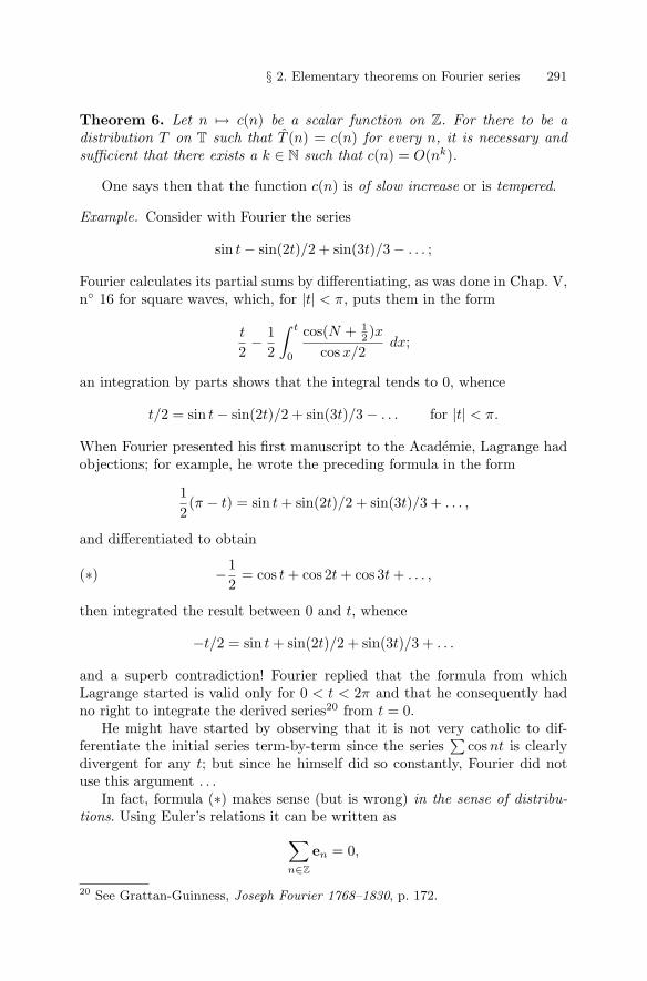
§ 2. Elementary theorems on Fourier series 291
Theorem 6. Let n → c(n) be a scalar function on Z. For there to be adistribution T on T such that T (n) = c(n) for every n, it is necessary andsufficient that there exists a k ∈ N such that c(n) = O(nk).
One says then that the function c(n) is of slow increase or is tempered.
Example. Consider with Fourier the series
sin t − sin(2t)/2 + sin(3t)/3 − . . . ;
Fourier calculates its partial sums by differentiating, as was done in Chap. V,n◦ 16 for square waves, which, for |t| < π, puts them in the form
t
2− 1
2
∫ t
0
cos(N + 12 )x
cos x/2dx;
an integration by parts shows that the integral tends to 0, whence
t/2 = sin t − sin(2t)/2 + sin(3t)/3 − . . . for |t| < π.
When Fourier presented his first manuscript to the Academie, Lagrange hadobjections; for example, he wrote the preceding formula in the form
12(π − t) = sin t + sin(2t)/2 + sin(3t)/3 + . . . ,
and differentiated to obtain
−12
= cos t + cos 2t + cos 3t + . . . ,(∗)
then integrated the result between 0 and t, whence
−t/2 = sin t + sin(2t)/2 + sin(3t)/3 + . . .
and a superb contradiction! Fourier replied that the formula from whichLagrange started is valid only for 0 < t < 2π and that he consequently hadno right to integrate the derived series20 from t = 0.
He might have started by observing that it is not very catholic to dif-ferentiate the initial series term-by-term since the series
∑cos nt is clearly
divergent for any t; but since he himself did so constantly, Fourier did notuse this argument . . .
In fact, formula (∗) makes sense (but is wrong) in the sense of distribu-tions. Using Euler’s relations it can be written as∑
n∈Z
en = 0,
20 See Grattan-Guinness, Joseph Fourier 1768–1830, p. 172.
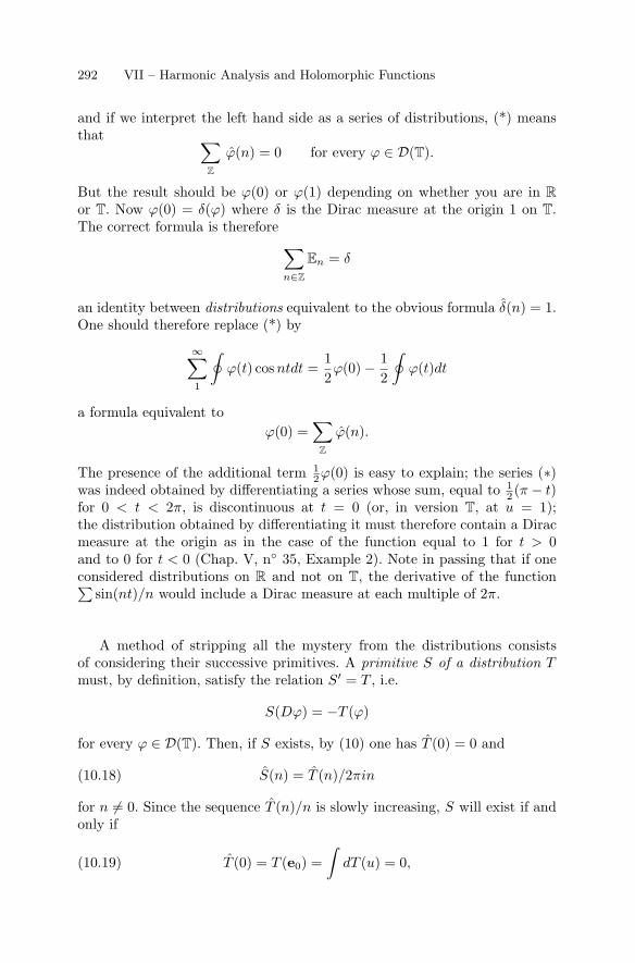
292 VII – Harmonic Analysis and Holomorphic Functions
and if we interpret the left hand side as a series of distributions, (*) meansthat ∑
Z
ϕ(n) = 0 for every ϕ ∈ D(T).
But the result should be ϕ(0) or ϕ(1) depending on whether you are in Ror T. Now ϕ(0) = δ(ϕ) where δ is the Dirac measure at the origin 1 on T.The correct formula is therefore∑
n∈Z
En = δ
an identity between distributions equivalent to the obvious formula δ(n) = 1.One should therefore replace (*) by
∞∑1
∮ϕ(t) cos ntdt =
12ϕ(0) − 1
2
∮ϕ(t)dt
a formula equivalent toϕ(0) =
∑Z
ϕ(n).
The presence of the additional term 12ϕ(0) is easy to explain; the series (∗)
was indeed obtained by differentiating a series whose sum, equal to 12 (π − t)
for 0 < t < 2π, is discontinuous at t = 0 (or, in version T, at u = 1);the distribution obtained by differentiating it must therefore contain a Diracmeasure at the origin as in the case of the function equal to 1 for t > 0and to 0 for t < 0 (Chap. V, n◦ 35, Example 2). Note in passing that if oneconsidered distributions on R and not on T, the derivative of the function∑
sin(nt)/n would include a Dirac measure at each multiple of 2π.
A method of stripping all the mystery from the distributions consistsof considering their successive primitives. A primitive S of a distribution Tmust, by definition, satisfy the relation S′ = T , i.e.
S(Dϕ) = −T (ϕ)
for every ϕ ∈ D(T). Then, if S exists, by (10) one has T (0) = 0 and
S(n) = T (n)/2πin(10.18)
for n �= 0. Since the sequence T (n)/n is slowly increasing, S will exist if andonly if
T (0) = T (e0) =∫
dT (u) = 0,(10.19)
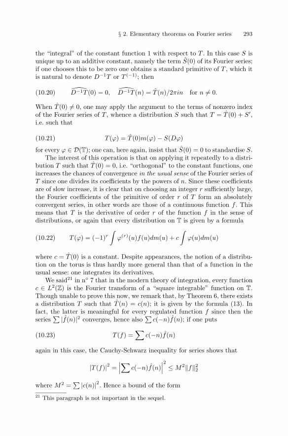
§ 2. Elementary theorems on Fourier series 293
the “integral” of the constant function 1 with respect to T . In this case S isunique up to an additive constant, namely the term S(0) of its Fourier series;if one chooses this to be zero one obtains a standard primitive of T , which itis natural to denote D−1T or T (−1); then
D−1T (0) = 0, D−1T (n) = T (n)/2πin for n �= 0.(10.20)
When T (0) �= 0, one may apply the argument to the terms of nonzero indexof the Fourier series of T , whence a distribution S such that T = T (0) + S′,i.e. such that
T (ϕ) = T (0)m(ϕ) − S(Dϕ)(10.21)
for every ϕ ∈ D(T); one can, here again, insist that S(0) = 0 to standardise S.The interest of this operation is that on applying it repeatedly to a distri-
bution T such that T (0) = 0, i.e. “orthogonal” to the constant functions, oneincreases the chances of convergence in the usual sense of the Fourier series ofT since one divides its coefficients by the powers of n. Since these coefficientsare of slow increase, it is clear that on choosing an integer r sufficiently large,the Fourier coefficients of the primitive of order r of T form an absolutelyconvergent series, in other words are those of a continuous function f . Thismeans that T is the derivative of order r of the function f in the sense ofdistributions, or again that every distribution on T is given by a formula
T (ϕ) = (−1)r
∫ϕ(r)(u)f(u)dm(u) + c
∫ϕ(u)dm(u)(10.22)
where c = T (0) is a constant. Despite appearances, the notion of a distribu-tion on the torus is thus hardly more general than that of a function in theusual sense: one integrates its derivatives.
We said21 in n◦ 7 that in the modern theory of integration, every functionc ∈ L2(Z) is the Fourier transform of a “square integrable” function on T.Though unable to prove this now, we remark that, by Theorem 6, there existsa distribution T such that T (n) = c(n); it is given by the formula (13). Infact, the latter is meaningful for every regulated function f since then theseries∑ |f(n)|2 converges, hence also
∑c(−n)f(n); if one puts
T (f) =∑
c(−n)f(n)(10.23)
again in this case, the Cauchy-Schwarz inequality for series shows that
|T (f)|2 =∣∣∣∑ c(−n)f(n)
∣∣∣2 ≤ M2‖f‖22
where M2 =∑ |c(n)|2. Hence a bound of the form
21 This paragraph is not important in the sequel.
294 VII – Harmonic Analysis and Holomorphic Functions
|T (f)| ≤ M‖f‖2 ≤ M‖f‖(10.24)
for every regulated function on T, and in particular for every continuousfunction, which shows that the distribution T is a measure on T. In fact, T isdefined by a measure of the form g(u)dm(u) where g is the square integrablefunction (a la Lebesgue) on T such that g(n) = c(n) for every n, and (24)is just the extension to these functions of the Cauchy-Schwarz inequality ofChap. V, n◦ 2.
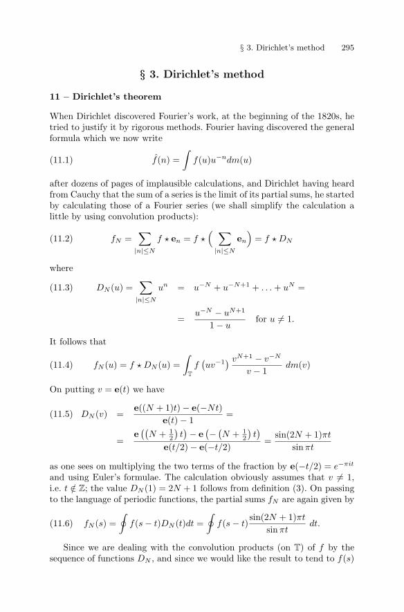
§ 3. Dirichlet’s method 295
§ 3. Dirichlet’s method
11 – Dirichlet’s theorem
When Dirichlet discovered Fourier’s work, at the beginning of the 1820s, hetried to justify it by rigorous methods. Fourier having discovered the generalformula which we now write
f(n) =∫
f(u)u−ndm(u)(11.1)
after dozens of pages of implausible calculations, and Dirichlet having heardfrom Cauchy that the sum of a series is the limit of its partial sums, he startedby calculating those of a Fourier series (we shall simplify the calculation alittle by using convolution products):
fN =∑
|n|≤N
f � en = f �( ∑
|n|≤N
en
)= f � DN(11.2)
where
DN (u) =∑
|n|≤N
un = u−N + u−N+1 + . . . + uN =(11.3)
=u−N − uN+1
1 − ufor u �= 1.
It follows that
fN (u) = f � DN (u) =∫
T
f(uv−1) vN+1 − v−N
v − 1dm(v)(11.4)
On putting v = e(t) we have
DN (v) =e((N + 1)t) − e(−Nt)
e(t) − 1=(11.5)
=e((
N + 12
)t)− e(− (N + 1
2
)t)
e(t/2) − e(−t/2)=
sin(2N + 1)πt
sin πt
as one sees on multiplying the two terms of the fraction by e(−t/2) = e−πit
and using Euler’s formulae. The calculation obviously assumes that v �= 1,i.e. t /∈ Z; the value DN (1) = 2N + 1 follows from definition (3). On passingto the language of periodic functions, the partial sums fN are again given by
fN (s) =∮
f(s − t)DN (t)dt =∮
f(s − t)sin(2N + 1)πt
sin πtdt.(11.6)
Since we are dealing with the convolution products (on T) of f by thesequence of functions DN , and since we would like the result to tend to f(s)
296 VII – Harmonic Analysis and Holomorphic Functions
when N increases indefinitely, it would seem, at first sight, that we shoulduse the method of Dirac sequences expounded in n◦ 5. The condition∫
DN (u)dm(u) =∮
DN (s)ds = 1
is satisfied, because this mean value is the Fourier coefficient of index 0 ofthe trigonometric polynomial DN . But the DN change sign more and moreoften as N increases; it is neither obvious (nor even correct) that the integralof |DN (u)| remains bounded as N increases. Finally, if one works on an arc|u − 1| > δ of T, then |DN (u)| ≤ ∣∣1 − u2N+1
∣∣ /δ by (3), which is insufficientto make DN (u) tend to 0. In short, a bad idea.
Moreover, if the DN did form a Dirac sequence, the Fourier series of everycontinuous function would converge uniformly to the latter by the lemma ofn◦ 5: this would be Paradise. On Earth, although converging “almost every-where” in the sense of Lebesgue measure22 (a famous and very difficult resultof Lars Carleson, 1966, valid for “square-integrable” functions in Lebesgue’ssense), it can still very well diverge for values of u forming an uncountableset23. In other words, the method does not work because if it did it wouldlead to a false result.
Having lived and died (1805–1859) too early to have heard of Lebesgue,Dirac, Carleson and even of Weierstrass’ approximation theorem, Dirichletdid not ask himself these questions and, using (4) – so in reality (5) – calcu-lated the difference
fN (u) − f(u) =∫ [
f(uv−1) − f(u)]DN (v)dm(v)(11.7)
or, replacing v by v−1 since DN is symmetric,
fN (u) − f(u) =∫
f(uv) − f(u)v − 1
(vN+1 − v−N
)dm(v)(11.8)
22 In Chap. V, n◦ 11 we defined the (Lebesgue) measure of an open U contained ina compact interval; n◦ 31, where we defined the integral of a positive lsc functionon R, likewise allowed us to define the measure of any open U ⊂ R. This beingso, a subset N of R is said to be of measure zero if for every r > 0 there exists anopen U such that N ⊂ U , m(U) < r. Granted this, a property – the convergenceof a series of functions for example – is said to be true almost everywhere if theset of x where it is false is of measure zero. Every countable set is of measurezero, but not conversely. See the Appendix to Chap. V.
23 The first example was that of the German P. du Bois-Reymond: “Before 1873, itwas the general belief, of Lejeune Dirichlet, of Riemann, of Weierstrass, amongothers, that this series always converges to the limit f(x) when f(x) is contin-uous. Now, in trying to find a proof of this theorem, I came upon an argumentto prove the contrary”. Letter of 1883 to the Frenchman G. Halphen (Dugac,p. 62). In 1926 the Soviet mathematician A. N. Kolmogoroff produced an in-tegrable (but not square integrable) function in the sense of Lebesgue whoseFourier series diverges everywhere. Newton would probably have said that onedoes not meet such functions in Nature.
§ 3. Dirichlet’s method 297
The right hand side of (8) resembles the difference between the Fourier coef-ficients of indices −N − 1 and N of the function
gu(v) = [f(uv) − f(u)]/(v − 1);(11.9)
but this function, as regulated as f for v �= 1, has, a priori, no meaningfor v = 1; its integral may well diverge on a neighbourhood of this point,which prevents one from speaking of its Fourier coefficients; the integral (8)is defined only because it involves the quotient
(vN+1 − v−N
)/(v − 1), an
everywhere continuous trigonometric polynomial.Since v − 1 = e(t) − 1 ∼ 2πit when t tends to 0, i.e. when v tends to 1,
one always has
lim[f(uv) − f(u)]/(v − 1) = f ′(s)/2πi(11.10)
if this derivative exists at the point u = e(s) considered. The function gu
then has left and right limit values at every point v ∈ T, so is regulated onall of T. In this case it is legitimate to write that
fN (u) − f(u) = gu(−N − 1) − gu(N);(11.11)
and to show that the left hand side tends to 0, it is enough to know that theFourier coefficients of a regulated function tend to 0 at infinity, which theParseval-Bessel inequality (7.12) makes obvious without recourse to Weier-strass’ theorem. Thus:
Theorem 7. Let f be a regulated periodic function. Then
f(u) =∑
f(n)un = limN→+∞
∑|n|≤N
f(n)un(11.12)
at every point u ∈ T where f is differentiable.
Corollary (Riemann). The behaviour on an open interval of the Fourierseries of a regulated periodic function f depends only on the behaviour of fon this interval.
If in fact f = g on an open interval U then the function f − g has aderivative at every point of U . Its Fourier series therefore converges to 0 atevery t ∈ U . This means that, for every t ∈ U , only two cases are possible:(i) the Fourier series of f and g are simultaneously divergent at t, (ii) theyare simultaneously convergent and have the same sum. Another translation:if two regulated periodic functions f and g are equal on an interval withcentre t, then their Fourier series at t are either simultaneously divergent, orsimultaneously convergent with the same sum on a neighbourhood of t.
Dirichlet in fact went somewhat further than Theorem 1, for the sum ofthe square wave series, to mention just this one, is not differentiable in the
298 VII – Harmonic Analysis and Holomorphic Functions
strict sense at the points where it is discontinuous; there it has only left andright derivatives; so one has to modify the preceding calculations. Now thesymmetry of the function DN shows that its integral over
[− 12 , 0]
or over[0, 1
2
]is equal to 1
2 ; this allows us to replace (7), or the R version, by
fN (s) − 12[f(s+) + f(s−)] =(11.13)
=∫ 1
2
0
[f(s + t) − f(s+)]DN (t)dt +∫ 1
2
0
[f(s − t) − f(s−)]DN (t)dt.
The quotient[f(s + t) − f(s+)]/ sin πt
appears in the first integral. If f has a right derivative at the point s (obviousdefinition), this quotient tends to a limit when t > 0 tends to 0; for 0 ≤ t ≤ 1
2 ,this quotient then has, like f , left and right limit values; the first integral isthus, as in (11), the value at N of the Fourier transform of a regulatedperiodic function that vanishes on
]12 , 1[, so tends to 0 as N increases. Same
argument for the second integral. Whence a simple result, which has beenrefined in many ways (see for example A. Zygmund, Trigonometrical Series,Cambridge UP, 1969):
Theorem 7 bis (Dirichlet, 1829). Let f be a regulated periodic functionand fN the partial sum of order N of its Fourier series. Then
lim fN (s) =12[f(s+) + f(s−)](11.14)
at every point where f has left and right derivatives.
Exercise Dirichlet’s Theorem is still valid if the function t → |f(s + t) −f(s)|/|t| is integrable. Example: f(s+ t) = f(s)+O(tα) when t → 0, with anα > 0, in which case the graph of f at s has a vertical tangent.
Example 1. Expansion of cot z as a series of rational fractions. Consider thefunction of period 1 on R given by
f(t) = cos 2πzt for |t| <12,(11.15)
where z ∈ C is not a rational integer, for otherwise there would be no problem.Since f
(− 12
)= f(
12
), the periodic function which extends f to all of R
is continuous everywhere and it is clear that it satisfies the hypotheses ofTheorem 7 bis. We have
f(n) =∫ 1
2
− 12
cos 2πzt.e−2πintdt =12
∫ 12
− 12
[e2πi(z−n)t + e−2πi(z+n)t
]dt =
=12
e2πi(z−n)t
2πi(z − n)+
e−2πi(z+n)t
−2πi(z + n)
∣∣∣∣12
− 12
= (−1)n z. sin πz
π(z2 − n2)
§ 3. Dirichlet’s method 299
as we see using Euler’s formulae. Thus
π. cos 2πzt =∑
(−1)n z. sin πz
z2 − n2e2πint for |t| ≤ 1
2,(11.16)
an absolutely convergent Fourier series. In particular, for t = 12 ,
π. cot πz = z∑ 1
z2 − n2=
1z
+ 2z∞∑
n=1
1z2 − n2
.(11.17)
This is the formula due to Euler which we have already met several times,and established at Chap. IV, n◦ 18, using the infinite product for the sinefunction. The method we have just presented – to be found essentially inFourier – is surely the simplest proof.
For t = 0, (16) yields the expansion
π
sin πz=
1z
+ 2z∑n≥1
(−1)n
z2 − n2.(11.18)
Example 2. The Bernoulli polynomials. Recall (Chap. VI, n◦ 12) that theBernoulli polynomials are defined by the recurrence relations
B0(x) = 1, B′k(x) = kBk−1(x)(11.19)
and by the condition
Bk(0) = Bk(1) for k ≥ 2.(11.20)
The inventor was not acquainted with Fourier series, but condition (20) isexactly what one needs to transform the Bk, for k ≥ 2, into continuousperiodic functions B∗
k , by putting
B∗k(t) = Bk(t) for 0 ≤ t ≤ 1(11.21)
as we did in Chap. VI a propos the Euler-Maclaurin formula. The hypothesesof the Dirichlet theorems are clearly satisfied. Adopting for once the notationan(f) = f(n), we have, integrating by parts and assuming k ≥ 2, n �= 0,
an (B∗k) =∫ 1
0
Bk(t)e−n(t)dt =1
2πin
∫ 1
0
B′k(t)e−n(t)dt;
(19) now shows that
an (B∗k) = kan
(B∗
k−1
)/2πin (k ≥ 2, n �= 0).(11.22)
On writing this relation for k − 1, k − 2, . . . , 2 we obtain
an (B∗k) = k!an (B∗
1) /(2πin)k−1.(11.23)
300 VII – Harmonic Analysis and Holomorphic Functions
Since B1(t) = t− 12 and since the Fourier coefficients of a constant vanish for
n �= 0, we have
an (B∗1) =∫ 1
0
te−n(t)dt = − te−n(t)2πin
∣∣∣∣10
+1
2πin
∫ 1
0
en(t)dt;
the last integral is zero and what remains is
an (B∗1) = −1/2πin,(11.24)
whence finally
an (B∗k) = −k!/(2πin)k for k ≥ 1, n �= 0.(11.25)
For n = 0, we have (k + 1)a0 (B∗k) =∮
B′k+1(t)dt = 0 by (20) if k ≥ 1, and
a0 (B∗0) = 1 trivially.
Formula (25) shows that the Fourier series is absolutely convergent fork ≥ 2, whence∑
n�=0
en(t)/(2πin)k = −Bk(t)/k! for k ≥ 2, 0 ≤ t ≤ 1,(11.26)
the sum being taken over all nonzero n ∈ Z. For k = 2 for example, one finds
∞∑1
cos(2πnt)/π2n2 = t2 − t + 1/6 (0 ≤ t ≤ 1).
For t = 0, the left hand side of (26) reduces to∑
1/(2πin)k, so is zero forodd k; for k = 2p, p ≥ 1, on the other hand,∑
1/n2p = (−1)p+1(2π)2pb2p/(2p)!(11.27)
where bk = Bk(0) (Chap. VI, (3.7)). We should not forget that the left handside is twice the sum of the Riemann series.
For k = 1, the function B∗1 , equal to t − 1
2 for 0 < t < 1, is discontinuousat the points t ∈ Z. On grouping the terms of index n and −n of its Fourierseries, we again have
12− t =
∞∑n=1
sin(2πnt)/πn for 0 < t < 1,(11.28)
the series being zero for t = 0 or 1 as one may check without invokingDirichlet. For t = 1
4 one obtains Leibniz’ series for π/4.
§ 3. Dirichlet’s method 301
12 – Fejer’s theorem
We observed in the preceding n◦ that the Dirichlet kernels do not form aDirac sequence in the sense of n◦ 5. At the end of the XIXth century, theItalian Cesaro had the idea of making divergent sequences (un) converge byconsidering their arithmetic means
vn = (u1 + . . . + un) /n.(12.1)
If you apply this to the sequence 1, 0, 1, 0, . . ., you will find that it then“converges” to 1
2 . The method does not always work, even if one iterates –every sequence which tends to +∞ is recalcitrant –, but it is reassuring atleast to know that if the sequence converges to u in the usual sense, then italso converges to u in the Cesaro sense: if |u − un| < r for n > p and if onewrites that
vn = (u1 + . . . + up) /n + (up+1 + . . . + un) /n,
the first quotient is, for p given, < r for n large; on replacing each uk by uin the second, one commits an error bounded by (n − p)r/n < r, whence atotal error < 2r for n large, qed.
One may also apply this procedure to a series∑
un, replacing the stan-dard partial sums sn = u1 + . . . + un by their means
σn = (s1 + . . . + sn) /n.(12.2)
This allows one to make convergent series which are not; one finds again, forexample, the formula
1 − 1 + 1 − 1 + 1 − . . . =12,
conforming to the somewhat premature anticipations of Jakob Bernoulli(Chap. II, n◦ 7). The subject has been the object of much research, butit is rarely used outside of “fine” analysis.
If one goes back to the Dirichlet formula
fN (t) =∮
f(t − x)DN (x)dx = f � DN (t)
for the partial sums of the Fourier series of a function f it is clear that theirarithmetic means are the functions f � FN where the function
FN = (D0 + . . . + DN−1) /N(12.3)
was introduced by L. Fejer (1880–1959).In contrast to the DN , the Fejer functions form a Dirac sequence on the
unit circle T. To see this, one has to calculate them. Putting q = eπit, onehas, by (10.5),
302 VII – Harmonic Analysis and Holomorphic Functions
Dk(t) =(q2k+1 − q−2k−1
)/(q − q−1
),
whence, adding from 0 to N − 1,
N(q − q−1
)FN (t) =
=(q + q3 + . . . + q2N−1
)− (q−1 + q−3 + . . . + q−2N+1)
=
= q(q2N − 1
)/(q2 − 1)− q−1
(q−2N − 1
)/(q−2 − 1
)=
=(q2N − 2 + q−2N
)/(q − q−1
)and finally
FN (t) =
(qN − q−N
)2N (q − q−1)2
=sin2 πNt
N sin2 πt,(12.4)
for t �= 0, with FN (0) = N by continuity or by (3).To show that the FN form a Dirac sequence on T it then suffices to show
that the FN are positive (obvious), that their integrals on T are equal to 1(obvious, since this is so for the Dk, hence for their arithmetic means) andfinally that, for any r > 0 and δ > 0, the contribution of the arc |u − 1| > δof T to the integral of FN is < r for N large or, equivalently, that∫
δ≤|t|≤1/2
FN (t)dt < r for N large.(12.5)
But on this domain of integration, by (4) one has
FN (t) ≤ 1/N sin2 πδ,(12.6)
so that the FN converge uniformly to 0 on δ ≤ |t| ≤ 12 for any δ > 0, qed.
Theorem 8 (Fejer). For every regulated periodic function f the arithmeticmeans of the partial sums of the Fourier series of f converge to 1
2 [f(t+) +f(t−)] for any t. If f is continuous in an open interval J , the convergenceto f(t) is uniform on every compact K ⊂ J .
The second assertion follows from the lemma of n◦ 5.To establish the first one writes, as in (11.13),
f � FN (t) − 12[f(t+) + f(t−)] =(12.7)
=∫
[f(t + s) − f(t+)]FN (s)ds +∫
[f(t − s) − f(t−)]FN (s)ds,
the integrals being taken over (0, 12 ), and then argues as in n◦ 5.
One may note in passing that assuming f continuous everywhere oneobtains a proof of Weierstrass’ approximation theorem (without having usedit beforehand . . .).
§ 3. Dirichlet’s method 303
Corollary. Let f be a regulated periodic function. Then
limN→∞
N∑−N
f(n)en(t) =12[f(t+) + f(t−)](12.8)
at every point where the Fourier series of f converges.
For the partial sums fN (t), if they converge, converge to the same limitas their arithmetic means, which always converge to the right hand side of(8). The corollary does not claim that the relation (8) is true for arbitrary tand f .
13 – Uniformly convergent Fourier series
Dirichlet’s theorem demonstrates the simple convergence of the Fourier seriesof a regulated periodic function at all points where it has left and right deriv-atives. In the case of the square waves we have shown by ad hoc calculations(Chap. III, n◦ 11) that in fact the series converges uniformly on every com-pact interval not containing discontinuities of f . One may refine the proof ofTheorem 7 so as to cover this case and many others, for example the series(11.28).
The arguments which follow being somewhat subtle, the reader is invitedto consider them more as an exercise.
Theorem 9. Let f be a regulated function on T and J an open arc on whichf is a primitive of a regulated function (is, for example, of class C1). Thenthe Fourier series of f converges to f uniformly on every compact arc K ⊂ J .
The proof we are going to set out calls on current techniques in functionalanalysis and can be divided into several stages.
(i) Consider again the function
gu(v) = [f(uv) − f(u)]/(v − 1)(∗)
that we used in proving Dirichlet’s theorem. As we saw then, gu is regulatedon T if f has left and right derivatives at u, so, under the hypotheses ofTheorem 9, for every u ∈ J . Then
fN (u) − f(u) = gu(−N − 1) − gu(N)
and the theorem reduces to showing that, as N → +∞, the functions
u → gu(N) = GN (u)
converge to 0 uniformly on every compact K of J , i.e. that for every r > 0there exists an N such that
304 VII – Harmonic Analysis and Holomorphic Functions
(u ∈ K) & (|n| > N) =⇒ |gu(n)| < r.(13.1)
(ii) Consider the vector space24 L1(T) of regulated functions on T, en-dowed with the norm ‖f‖1 =
∫ |f(v)|dm(v). Then gu ∈ L1(T) for everyu ∈ J , and the simplest estimate for the Fourier coefficients of an integrablefunction shows that
|Gn(u′) − Gn(u′′)| = |gu′(n) − gu′′(n)| ≤ ‖gu′ − gu′′‖1(13.2)
for any u′ and u′′ ∈ J .Suppose we have shown that the map u → gu of J in L1(T) is continuous,
i.e. that for every u ∈ J and every r > 0 there exists an r′ > 0 such that
(u′ ∈ J) & (|u′ − u| < r′) =⇒ ‖gu′ − gu‖1 < r.(13.3)
The relation (2) then shows that
(u′ ∈ J) & (|u′ − u| < r′) =⇒ |Gn(u′) − Gn(u)| < r for every n.(13.4)
This means precisely that the functions Gn are equicontinuous on J (Chap. III,n◦ 5). The fact that the Gn(u) converge to 0 uniformly on every compactK ⊂ J will then follow from the following general lemma:
Lemma. If a sequence of functions fn defined and equicontinuous on a com-pact set K converges simply on K, then it converges uniformly on K.
Suppose that f is the limit of the fn and let us choose an r > 0. For everya ∈ K there exists an open ball B(a) with centre a in K such that
x ∈ B(a) =⇒ |fn(x) − fn(a)| ≤ r for every n;
this is the definition of equicontinuity. The inequality remains valid for f bypassage to the limit, which proves the continuity of f ; since |fn(a) − f(a)| ≤ rfor n large one deduces that, for n large,
|f(x) − fn(x)| ≤ 3r
for every x ∈ B(a). But, since K is compact, one may (Borel-Lebesgue) coverit by a finite number of balls B(ai). The above inequality is then, for n large,valid on all these balls, so on K, qed.
(iii) To prove the continuity of the map u → gu of J into L1(T), let usfirst consider, in this part of the proof, the numerator f(uv) − f(u) of (∗).This is the difference between, on the one hand, the function fu : v → f(uv)obtained by “translating” the function f , and on the other hand the constant24 The authentic L1 space in Lebesgue theory contains many other functions, but,
since it certainly contains the regulated functions, this is what we deal with here.
§ 3. Dirichlet’s method 305
function cu : v → f(u). Since ‖cu′ − cu′′‖1 = |f(u′) − f(u′′)|, it is clear thatu → cu is a continuous map of J into L1(T).
As for u → fu, this is a continuous map of T (and not only of J)into L1(T). This is obvious if f is continuous on T, for f being now uni-formly continuous on T, we have |f(u′v) − f(u′′v)| ≤ r for every v ∈ T,so also ‖fu′ − fu′′‖1 ≤ r so long as |u′ − u′′| < r′. In the general case, wemay choose, thanks to the lemma of n◦ 8, a function ϕ ∈ C0(T) such that∫ |f(v) − ϕ(v)|dm(v) = ‖f − ϕ‖1 < r. Since we are integrating with respectto an invariant measure, we again have ‖fu − ϕu‖1 < r for every u ∈ T. Ifwe now choose functions ϕ ∈ C0(T) which converge to f in L1(T), the cor-responding maps u → ϕu of T into L1(T) converge to u → fu uniformly onT. A uniform limit of continuous functions with values in any metric spacebeing again continuous, the required result follows.
So we see that the numerator of the formula (∗), considered as a functionof u ∈ J with values in L1(T), is continuous.
(iv) Next we have to take account of the denominator v − 1 and, to dothis, use our hypotheses. We shall first give the proof in the case where f = 0on J ; and show later that the general case reduces to this.
Since the compact sets K and T − J are disjoint their distance d is > 0.Since |uv − u| = |v − 1|, we see that
(u ∈ K) & (|v − 1| < d) =⇒ uv ∈ J(13.5)=⇒ f(uv) = f(u) = 0.
When we restrict to the u ∈ K, the functions of v appearing in the numeratorof the formula (∗) are thus all zero on the arc |v − 1| < d of T. Let us put
h(v) = (v − 1)−1 if |v − 1| > d, h(v) = 0 if not.(13.6)
The formula that defines gu shows that, for u ∈ K,
gu(v) = h(v) [fu(v) − cu(v)] for every v ∈ T.(13.7)
This is essentially the definition of gu on the arc |v − 1| > d and, by (5),reduces to the identity 0 = 0 on the arc |v − 1| < d.
Now we have |h(v)| < 1/d for any v ∈ T by (6). The relation (7) showingthat gu = h (fu − cu) for u ∈ K (though not for every u ∈ T) and the mapu → fu − cu of T into L1(T) being continuous, by point (iii), it remains toshow that multiplication by the function h, which is bounded and independentof u, preserves continuity. This is no more difficult than in the framework ofcomplex valued functions: it is enough to write that
‖hf ′ − hf ′′‖1 =∫
|h(v)|.|f ′(v) − f ′′(v)|dm(v) ≤ ‖h‖. ‖f ′ − f ′′‖1
for any f ′, f ′′ ∈ L1(T), where ‖h‖ = sup |h(v)| as always. Since, for u′, u′′ ∈ Ksufficiently close, the distance from f ′ = fu′ − cu′ to f ′′ = fu′′ − cu′′ is
306 VII – Harmonic Analysis and Holomorphic Functions
arbitrarily small, so likewise is the distance from gu′ to gu′′ , which proves thetheorem in the case where f = 0 in J .
(v) It remains to pass to the general case. The arc K being compact, andthe arc J open, the distance d of K to the compact T − J is > 0, so thatthe open arc J ′ of T defined by d(u,K) < d/2 satisfies K ⊂ J ′ ⊂ J . Bymodifying the graph of f outside J ′ one may construct a function g which,on all of T, is a primitive of a regulated function and which, on J ′, coincideswith f . Since f − g vanishes on J ′ its Fourier series converges uniformly to 0on K by section (iv) of the proof. Now the Fourier series of g converges to guniformly in T (n◦ 9, Theorem 4) and so to f uniformly on K. The relationf = (f − g) + g then completes the proof.

§ 4. Analytic and holomorphic functions 307
§ 4. Analytic and holomorphic functions
In Chap. II, n◦ 19, which the reader is strongly urged to review, we said thata function f defined on an open subset U of C is analytic in U if for everya ∈ U there exists a power series in z − a which, on a sufficiently small discof centre a, converges to f(z). In fact it represents f(z) in the largest discD ⊂ U where it converges, for the sum of this power series is analytic inits disc of convergence (Chap. II, n◦ 19, Theorem 14) and since it is equalto f on a neighbourhood of the centre of D, it is equal to f everywhere inD by virtue of the principle of analytic continuation (Chap. II, n◦ 20); thesame argument shows that the one and only power series representing f on aneighbourhood of a is the Taylor series of f at a. We know that it converges,but we still do not know up to where it converges . . .
We have also shown that, if the function f is analytic, it has a derivative
f ′(a) = lim[f(a + h) − f(a)]/h(∗)
in the complex sense at each point a ∈ U ; the latter can also be obtainedby differentiating the power series representing f term-by-term on a neigh-bourhood of a. The existence of the limit (∗) shows that as a function of thereal variables x = Re(z) and y = Im(z) the function f has partial derivativessatisfying the Cauchy formula
D2f = iD1f (= if ′).(∗∗)
On the other hand we have shown (Chap. III, n◦ 20, corollary of Theorem 21)that, conversely, every holomorphic function, i.e. possessing continuous par-tial derivatives satisfying (∗∗) in an open set U , has a complex derivative (∗)and that its differential can be written in the form
df = f ′(z)dz = f ′(z)(dx + idy).(∗ ∗ ∗)
In the following n◦ we shall show that a holomorphic function is necessar-ily analytic, by a method that exploits Fourier series, after which the terms“analytic” and “holomorphic” will become synonymous, as we have alreadyannounced several times in earlier chapters. Then we shall expound the sim-plest consequences of this result, without seeking to enter into the detail of atheory to which hundreds of mathematicians have, since Cauchy, added theircontribution from their grain of sand to the Empire State Building; Rem-mert’s two volumes, 650 very condensed pages, can scarcely cover the ellipticfunctions and not at all the modular and automorphic functions, Riemannsurfaces, analytic differential equations, special functions, etc., not to speakof the generalisations to several variables.
308 VII – Harmonic Analysis and Holomorphic Functions
14 – Analyticity of the holomorphic functions
Having recalled these preliminaries let us consider a function f(z) definedand holomorphic on an open disc D : |z| < R. We would like to show that itis represented in all this disc by a power series
f(z) =∑
anzn.(14.1)
As we have seen in n◦ 1 of this chapter, or in Chap. V, n◦ 5, this essentiallyreduces to showing that the function
an(r) =∫
f(ru)u−ndm(u)(14.2)
is, for every n ∈ Z, proportional to rn, using only the Cauchy condition or,equivalently, the existence and the continuity of f ′(z).
In this direction we write
an(r) =∫ 1
0
f [re(t)]e−n(t)dt(14.3)
and calculate the derivative of an(r). We have to perform a differentiationunder the
∫sign, an operation examined in Chap. V, n◦ 9, Theorem 9: this
is permitted if the function of r and t that one is integrating has a partialderivative with respect to r and if the latter is a continuous function of thepair (r, t). The factor e−n(t) poses no problem. The factor f [re(t)] neither: fis C1 and, for t given, the map r → re(t) is C∞. The general relation (21.2)of Chap. III, n◦ 21, namely that
d
drf [g(r)] = f ′[g(r)]g′(r),(14.4)
valid if f is holomorphic and if g is a C1 function of the real variable r, thenshows that in our case
d
drf [re(t)] = f ′[re(t)]
d
drre(t) = f ′[re(t)]e(t)(14.5)
is a continuous function of the pair (r, t). Thus
d
dran(r) =
∫ 1
0
f ′[re(t)]e(t)e−n(t)dt.(14.6)
Since on the other hand, by the same argument,
d
dtf [re(t)] = f ′[re(t)]
d
dtre(t) = 2πirf ′[re(t)]e(t),(14.7)
(6) can again be written
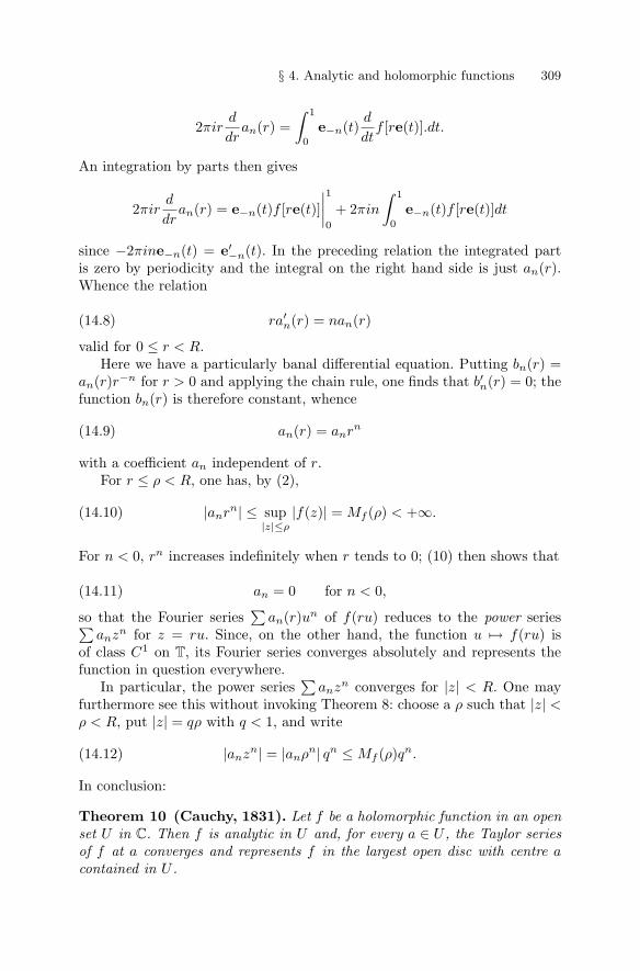
§ 4. Analytic and holomorphic functions 309
2πird
dran(r) =
∫ 1
0
e−n(t)d
dtf [re(t)].dt.
An integration by parts then gives
2πird
dran(r) = e−n(t)f [re(t)]
∣∣∣∣10
+ 2πin
∫ 1
0
e−n(t)f [re(t)]dt
since −2πine−n(t) = e′−n(t). In the preceding relation the integrated partis zero by periodicity and the integral on the right hand side is just an(r).Whence the relation
ra′n(r) = nan(r)(14.8)
valid for 0 ≤ r < R.Here we have a particularly banal differential equation. Putting bn(r) =
an(r)r−n for r > 0 and applying the chain rule, one finds that b′n(r) = 0; thefunction bn(r) is therefore constant, whence
an(r) = anrn(14.9)
with a coefficient an independent of r.For r ≤ ρ < R, one has, by (2),
|anrn| ≤ sup|z|≤ρ
|f(z)| = Mf (ρ) < +∞.(14.10)
For n < 0, rn increases indefinitely when r tends to 0; (10) then shows that
an = 0 for n < 0,(14.11)
so that the Fourier series∑
an(r)un of f(ru) reduces to the power series∑anzn for z = ru. Since, on the other hand, the function u → f(ru) is
of class C1 on T, its Fourier series converges absolutely and represents thefunction in question everywhere.
In particular, the power series∑
anzn converges for |z| < R. One mayfurthermore see this without invoking Theorem 8: choose a ρ such that |z| <ρ < R, put |z| = qρ with q < 1, and write
|anzn| = |anρn| qn ≤ Mf (ρ)qn.(14.12)
In conclusion:
Theorem 10 (Cauchy, 1831). Let f be a holomorphic function in an openset U in C. Then f is analytic in U and, for every a ∈ U , the Taylor seriesof f at a converges and represents f in the largest open disc with centre acontained in U .
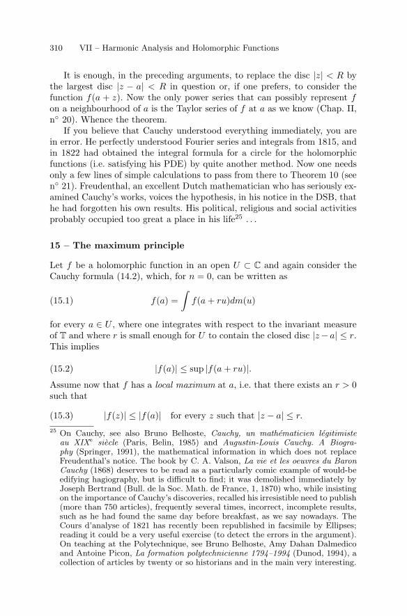
310 VII – Harmonic Analysis and Holomorphic Functions
It is enough, in the preceding arguments, to replace the disc |z| < R bythe largest disc |z − a| < R in question or, if one prefers, to consider thefunction f(a + z). Now the only power series that can possibly represent fon a neighbourhood of a is the Taylor series of f at a as we know (Chap. II,n◦ 20). Whence the theorem.
If you believe that Cauchy understood everything immediately, you arein error. He perfectly understood Fourier series and integrals from 1815, andin 1822 had obtained the integral formula for a circle for the holomorphicfunctions (i.e. satisfying his PDE) by quite another method. Now one needsonly a few lines of simple calculations to pass from there to Theorem 10 (seen◦ 21). Freudenthal, an excellent Dutch mathematician who has seriously ex-amined Cauchy’s works, voices the hypothesis, in his notice in the DSB, thathe had forgotten his own results. His political, religious and social activitiesprobably occupied too great a place in his life25 . . .
15 – The maximum principle
Let f be a holomorphic function in an open U ⊂ C and again consider theCauchy formula (14.2), which, for n = 0, can be written as
f(a) =∫
f(a + ru)dm(u)(15.1)
for every a ∈ U , where one integrates with respect to the invariant measureof T and where r is small enough for U to contain the closed disc |z−a| ≤ r.This implies
|f(a)| ≤ sup |f(a + ru)|.(15.2)
Assume now that f has a local maximum at a, i.e. that there exists an r > 0such that
|f(z)| ≤ |f(a)| for every z such that |z − a| ≤ r.(15.3)25 On Cauchy, see also Bruno Belhoste, Cauchy, un mathematicien legitimiste
au XIXe siecle (Paris, Belin, 1985) and Augustin-Louis Cauchy. A Biogra-phy (Springer, 1991), the mathematical information in which does not replaceFreudenthal’s notice. The book by C. A. Valson, La vie et les oeuvres du BaronCauchy (1868) deserves to be read as a particularly comic example of would-beedifying hagiography, but is difficult to find; it was demolished immediately byJoseph Bertrand (Bull. de la Soc. Math. de France, 1, 1870) who, while insistingon the importance of Cauchy’s discoveries, recalled his irresistible need to publish(more than 750 articles), frequently several times, incorrect, incomplete results,such as he had found the same day before breakfast, as we say nowadays. TheCours d’analyse of 1821 has recently been republished in facsimile by Ellipses;reading it could be a very useful exercise (to detect the errors in the argument).On teaching at the Polytechnique, see Bruno Belhoste, Amy Dahan Dalmedicoand Antoine Picon, La formation polytechnicienne 1794–1994 (Dunod, 1994), acollection of articles by twenty or so historians and in the main very interesting.
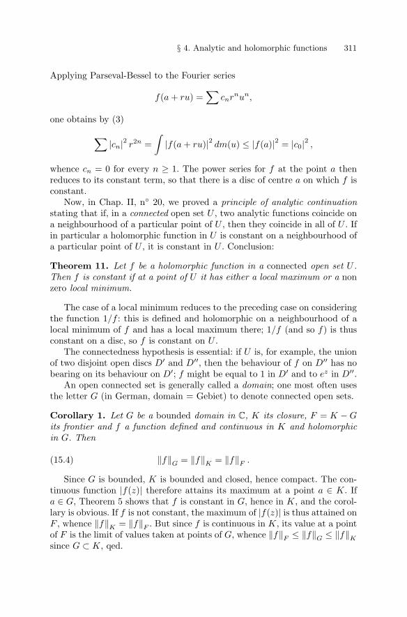
§ 4. Analytic and holomorphic functions 311
Applying Parseval-Bessel to the Fourier series
f(a + ru) =∑
cnrnun,
one obtains by (3)
∑|cn|2 r2n =
∫|f(a + ru)|2 dm(u) ≤ |f(a)|2 = |c0|2 ,
whence cn = 0 for every n ≥ 1. The power series for f at the point a thenreduces to its constant term, so that there is a disc of centre a on which f isconstant.
Now, in Chap. II, n◦ 20, we proved a principle of analytic continuationstating that if, in a connected open set U , two analytic functions coincide ona neighbourhood of a particular point of U , then they coincide in all of U . Ifin particular a holomorphic function in U is constant on a neighbourhood ofa particular point of U , it is constant in U . Conclusion:
Theorem 11. Let f be a holomorphic function in a connected open set U .Then f is constant if at a point of U it has either a local maximum or a nonzero local minimum.
The case of a local minimum reduces to the preceding case on consideringthe function 1/f : this is defined and holomorphic on a neighbourhood of alocal minimum of f and has a local maximum there; 1/f (and so f) is thusconstant on a disc, so f is constant on U .
The connectedness hypothesis is essential: if U is, for example, the unionof two disjoint open discs D′ and D′′, then the behaviour of f on D′′ has nobearing on its behaviour on D′; f might be equal to 1 in D′ and to ez in D′′.
An open connected set is generally called a domain; one most often usesthe letter G (in German, domain = Gebiet) to denote connected open sets.
Corollary 1. Let G be a bounded domain in C, K its closure, F = K − Gits frontier and f a function defined and continuous in K and holomorphicin G. Then
‖f‖G = ‖f‖K = ‖f‖F .(15.4)
Since G is bounded, K is bounded and closed, hence compact. The con-tinuous function |f(z)| therefore attains its maximum at a point a ∈ K. Ifa ∈ G, Theorem 5 shows that f is constant in G, hence in K, and the corol-lary is obvious. If f is not constant, the maximum of |f(z)| is thus attained onF , whence ‖f‖K = ‖f‖F . But since f is continuous in K, its value at a pointof F is the limit of values taken at points of G, whence ‖f‖F ≤ ‖f‖G ≤ ‖f‖K
since G ⊂ K, qed.
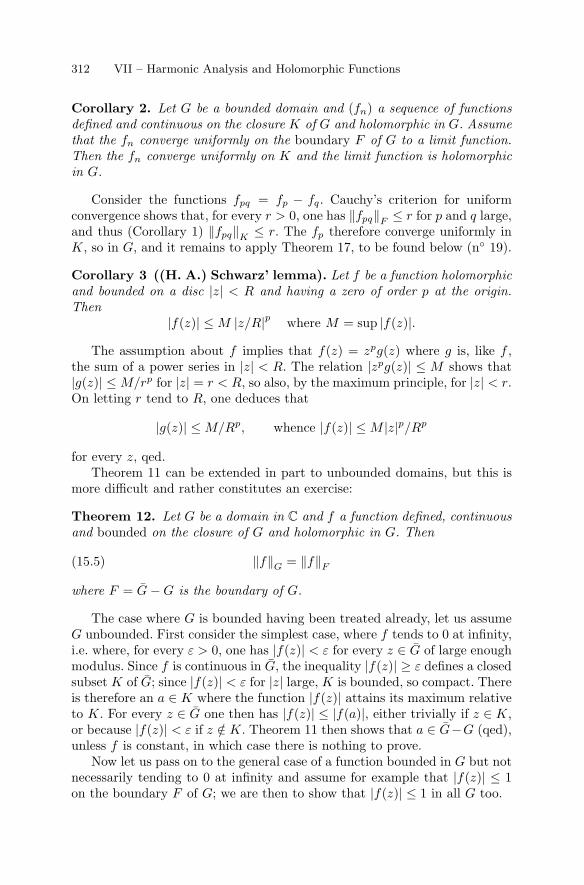
312 VII – Harmonic Analysis and Holomorphic Functions
Corollary 2. Let G be a bounded domain and (fn) a sequence of functionsdefined and continuous on the closure K of G and holomorphic in G. Assumethat the fn converge uniformly on the boundary F of G to a limit function.Then the fn converge uniformly on K and the limit function is holomorphicin G.
Consider the functions fpq = fp − fq. Cauchy’s criterion for uniformconvergence shows that, for every r > 0, one has ‖fpq‖F ≤ r for p and q large,and thus (Corollary 1) ‖fpq‖K ≤ r. The fp therefore converge uniformly inK, so in G, and it remains to apply Theorem 17, to be found below (n◦ 19).
Corollary 3 ((H. A.) Schwarz’ lemma). Let f be a function holomorphicand bounded on a disc |z| < R and having a zero of order p at the origin.Then
|f(z)| ≤ M |z/R|p where M = sup |f(z)|.The assumption about f implies that f(z) = zpg(z) where g is, like f ,
the sum of a power series in |z| < R. The relation |zpg(z)| ≤ M shows that|g(z)| ≤ M/rp for |z| = r < R, so also, by the maximum principle, for |z| < r.On letting r tend to R, one deduces that
|g(z)| ≤ M/Rp, whence |f(z)| ≤ M |z|p/Rp
for every z, qed.Theorem 11 can be extended in part to unbounded domains, but this is
more difficult and rather constitutes an exercise:
Theorem 12. Let G be a domain in C and f a function defined, continuousand bounded on the closure of G and holomorphic in G. Then
‖f‖G = ‖f‖F(15.5)
where F = G − G is the boundary of G.
The case where G is bounded having been treated already, let us assumeG unbounded. First consider the simplest case, where f tends to 0 at infinity,i.e. where, for every ε > 0, one has |f(z)| < ε for every z ∈ G of large enoughmodulus. Since f is continuous in G, the inequality |f(z)| ≥ ε defines a closedsubset K of G; since |f(z)| < ε for |z| large, K is bounded, so compact. Thereis therefore an a ∈ K where the function |f(z)| attains its maximum relativeto K. For every z ∈ G one then has |f(z)| ≤ |f(a)|, either trivially if z ∈ K,or because |f(z)| < ε if z /∈ K. Theorem 11 then shows that a ∈ G−G (qed),unless f is constant, in which case there is nothing to prove.
Now let us pass on to the general case of a function bounded in G but notnecessarily tending to 0 at infinity and assume for example that |f(z)| ≤ 1on the boundary F of G; we are then to show that |f(z)| ≤ 1 in all G too.
§ 4. Analytic and holomorphic functions 313
Assume |f(a)| > 1 for some a ∈ G and consider a closed disc D : |z − a| ≤ rcontained in G. Theorem 11 shows that the maximum M of |f | on the bound-ary of D is > 1. Consider now in the domain H = G − D the functions
fn(z) = rf(z)n/Mn(z − a).(15.6)
Since f is bounded in G, the introduction of a denominator z− a shows thatthe fn tend to 0 at infinity in H. One is therefore in the particular caseexamined first. Now the boundary of H is clearly the union of the boundaryF of G and that of the disc D. On F , by hypothesis |f(z)| ≤ 1, and sinceM and |(z − a)/r| are >1, one has |fn(z)| ≤ 1 on F . The same result holdson the boundary of D since there |f(z)| ≤ M and |z − a| = r. Thus we seethat the function |fn(z)| is ≤ 1 on the boundary of H, and since it tends to 0at infinity we conclude that |fn(z)| ≤ 1 in H. The exponent n in (6) beingarbitrary, this forces |f(z)/M | ≤ 1 in H. This relation also being satisfied inD, it holds everywhere in G, qed.
The hypothesis that the function f is bounded in G and not only on itsboundary is essential in the above. All this has been prodigiously refined.
16 – Functions analytic in an annulus. Singular points. Meromor-phic functions
The arguments of n◦ 14 in fact apply to a function defined in an annulusC : R1 < |z| < R2 and in particular on a disc with its centre deleted ifR1 = 0. For every circle |z| = r contained in C the Fourier coefficients of thefunction f(ru) are again of the form anrn, but the argument showing thatan = 0 for n < 0 no longer applies since, even in the case where R1 = 0, thefunction, for example 1/z, has no reason to be bounded on a neighbourhoodof 0. What survives is the Fourier series of f(ru), namely
∑anrnun =
∑anzn with anrn =
∫f(ru)u−ndm(u),(16.1)
where this time the sum is extended over Z, converges absolutely and repre-sents f in C by Theorem 4 of n◦ 9. Here again, one may see the convergencedirectly. Let us choose numbers r1 and r2 such that R1 < r1 < |z| < r2 < R2
(strict inequalities) and let M be the uniform norm of f on the compactannulus C ′ delimited by the circles of radii r1 and r2. Now |anzn| ≤ M by(1), since |f(ru)| ≤ M , whence
|anzn| ={ |anrn
2 | . |z/r2|n < M |z/r2|n for n ≥ 0,|anrn
1 | . |z/r1|n < M |z/r1|n for n ≤ 0;(16.2)
since |z/r2| < 1, the first inequality proves the absolute convergence of the“positive” part of the series (1), and since |z/r1| > 1, the second proves thatof its “negative” part.

314 VII – Harmonic Analysis and Holomorphic Functions
The series (1) even converges normally in C ′ and so on every compact26
K ⊂ C. Thus, in C ′,
|anzn| ≤{ |anrn
1 | if n ≥ 0|anrn
2 | if n < 0;
now we know that the series∑
anzn converges absolutely in C, thus forz = r1 or r2; whence, in C ′, a bound by a convergent series independent of z.In conclusion:
Theorem 13 (Laurent). Let f be a holomorphic function in an annulusC : R1 < |z| < R2. Then we have a series expansion
f(z) =∑n∈Z
anzn with an = r−n
∫T
f(ru)u−ndm(u),(16.3)
the series converging normally on every compact K ⊂ C.
An expansion of this type is called a Laurent series; it is the sum of apower series in z and of a power series in 1/z. The first converges at least for|z| < R2 and the second for |z| > R1 since a power series necessarily convergeson a disc. This allows us to write that, in C, we have a decomposition f(z) =g(z) + h(z) of f into a function g holomorphic for |z| < R2 and a function hholomorphic for |z| > R1.
We may write (16.3) a la Leibniz like the Cauchy formula of n◦ 1. Puttingζ = ru we have an =
∫f(ζ)ζ−ndm(u); but for u = e(t) we have dζ =
2πire(t)dt = 2πiζdm(u). Whence
2πian =∫
f(ζ)ζ−n−1dζ,
the “line” integral being taken along any circle t → re(t) contained in C.Cauchy’s theory will illuminate this point and, in particular, will explainwhy the result is independent of the circle |ζ| = r chosen.
Theorem 13 serves mainly to study the behaviour of a holomorphic func-tion on a neighbourhood of an isolated singular point a, i.e. of a function de-fined and holomorphic on a neighbourhood of a, except at the point a itself.There one has a series expansion f(z) =
∑cn(z−a)n, whence the distinction
between the poles, where the series includes only finite number of nonzeroterms of degree < 0 – the minimal degree, its sign changed, is called the orderof the pole in question –, and the essential singular points where it includes26 Such a compact subset is contained in C′ if one chooses the radii r1 and r2
suitably: the continuous real function z �→ |z| attains its minimum and its maxi-mum on K, which are strictly contained between the radii of C since the limitingcircles of C, which do not lie in C, do not meet K.
§ 4. Analytic and holomorphic functions 315
infinitely many, the case for example of the function exp(1/z) =∑
z−n/n! atz = 0. It is also useful to define the order of a zero a of f , i.e. of a point wheref(a) = 0: this is the degree of the first nonzero term of the power series of fat a.
This leads to the fundamental concept of a function meromorphic in anopen set U : this is a function f defined and analytic in U − D, where Dis a discrete subset of U (i.e. such that, for every a ∈ U , there exists adisc of centre a containing a finite number of points of D), and having onlypolar singularities at the points of D. This, for example, is the case of theelliptic functions of Chap. II, n◦ 23 and, in fact, the “right” definition of theelliptic functions, for there are many, other than the Eisenstein series, is toimpose on them just that they should be simultaneously doubly periodic andmeromorphic in C, as Liouville discovered (n◦ 18).
We note that, if D′ is the set of zeros of a meromorphic function f in U ,then the union D ∪ D′ is again a discrete subset of U . This results from thefact that, if a is any point in U , then f(z) = (z−a)pg(z), where g is a powerseries whose constant term is not zero, so such that g(a) �= 0; on a smallenough disc of centre a we again have g(z) �= 0 since g is continuous, so thaton a neighbourhood of a the function f can have no other zero or pole thanthe point a itself. On the other hand, the zeros or poles of a function havingan essential singular point at a may accumulate at a: the zeros of sin(1/z)converge to 0.
One may perform the usual algebraic operations on the functions mero-morphic in a given open set U : sum, product, quotient; as we shall see, oneagain obtains meromorphic functions in U .
The case of a sum f + g is obvious: if f and g have poles at the pointsof two discrete subsets D and D′ of U , the function f + g is holomorphicoutside D ∪ D′ and it is clear that at a point of D ∪ D′ it has at most apole; “at most” because the polar parts of the Laurent series of f and g ata common pole may cancel each other. For fg, holomorphic outside D ∪D′,one observes that at a point a ∈ D ∪ D′ one has the relations
f(z) = f1(z)/(z − a)p, g(z) = g1(z)/(z − a)q
where f1 and g1 are holomorphic on a neighbourhood of a and nonzero at a.It is then clear that fg has a pole of order p+q at a. Of course it can happenthat a pole of f is neutralised by a zero of g.
The case of the quotient f/g reduces, as always, to that of the reciprocal1/g(z) of a meromorphic function. On a neighbourhood of a pole a of g onehas g(z) = g1(z)/(z − a)q where g1(z) is a power series such that g1(a) �= 0.The function g1 has a reciprocal 1/g1(z) holomorphic on a neighbourhoodof a; the formula 1/g(z) = (z − a)q/g1(z) then shows that the pole a oforder q is transformed into a zero of order q of 1/g(z). At a point a where gis holomorphic one has g(z) = (z − a)qg1(z) where g1 is a power series notvanishing at a, whose reciprocal is thus holomorphic on a neighbourhood
316 VII – Harmonic Analysis and Holomorphic Functions
of a, whence clearly a pole of order q for 1/g(z) if g has a zero of order qat a. Finally we see that 1/g(z) is holomorphic outside the zeros of g, whichare the poles of 1/g, the poles of g contrariwise providing the zeros of 1/g.Since the zeros of g form a discrete set in U , the function 1/g is thereforemeromorphic in U .
Laurent series can be manipulated like power series. The domain of con-vergence of a series such as f(z) =
∑anzn is necessarily an annulus C since
it is the sum of a power series in z and of a power series in 1/z which convergefor |z| < R2 and |1/z| < R1 respectively. The multiplication formula∑
anzn∑
bnzn =∑
cnzn with cn =∑
apbn−p
valid for power series still applies, restricted to an annulus where the twoseries converge: they then converge absolutely, therefore unconditionally, soon multiplying term-by-term one obtains a double series
∑apbqz
p+q whichconverges unconditionally (Chap. II, n◦ 22) and in which one may reorder theterms arbitrarily (Chap. II, n◦ 18, Theorem 13: associativity), for exampleas a function of the value of p + q.
One may also differentiate a Laurent series term-by-term; the simplestway to see this is to write f(z) = g(z) + h(1/z) where g and h are powerseries, whence
f ′(z) = g′(z) − h′(1/z)/z2
by the chain rule for analytic functions (Chap. II, n◦ 22, Theorem 17);as we know, g′(z) is obtained by differentiating the “positive” part of theseries
∑anzn term-by-term; since h(z) =
∑n≥0 a−nzn and so h′(z) =∑
n≥0 na−nzn−1, it follows that
h′(1/z)/z2 =∑n≥0
na−nz−n+1−2 =∑n≥0
na−nz−n−1 = −∑n≤0
nanzn−1
and finally
f ′(z) =∑n≥0
nanzn−1 +∑n≤0
nanzn−1 =∑
nanzn−1
as one had hoped, the Laurent series of f ′ converging in the same annulus Cas f . Note that there is no term in 1/z in the result.
An essential difference from power series will appear when one looks fora primitive of f , i.e. a holomorphic function F such that F ′(z) = f(z) inC. The function F is, like f , represented by a Laurent series and as wehave just seen the derived series contains no term in 1/z. The problem cantherefore have no solution if the series f(z) contains one. The analogousproblem for a real variable had, in the XVIIth century, defied the efforts ofseveral mathematicians before Newton and Mercator, and Newton himself,
§ 4. Analytic and holomorphic functions 317
with his systematic use of Laurent series having a finite number of terms ofnegative degree, is very reticent on this subject. This “detail”, on which thewhole of Cauchy’s “residue calculus” is founded, apart, the existence of theprimitive when a−1 = 0 is as obvious as for the case of power series: oneputs F (z) =
∑anzn+1/(n + 1). The arguments employed for power series in
Chap. II, n◦ 19 or, equivalently, the fact that in the domain C of convergenceof the series, the an of positive index and those of negative index are boundedby geometric progressions, show that these operations – differentiation or“integration” term-by-term – lead to series converging in the same annulusas the initial series.
In the case where f contains a term in 1/z, one may again consider thefunction F (z) =
∑anzn+1/(n + 1), where one forgets the term of index
n = −1; instead of f = F ′ one obtains the relation
f(z) = F ′(z) + a−1/z.(16.4)
The coefficient a−1, the radical obstruction to the existence of a primitive off in the annulus C, is called the residue of f ; more generally, if one considersa function f holomorphic on a neighbourhood of a point c of C except atthe point itself, which is then an isolated singular point of f , the residue off at c is by definition the coefficient a−1 of 1/(z − c) in the expansion of fas a Laurent series
∑an(z − c)n about the point c; one writes Resc(f) or
Res(f, c). The formula (3) applied for n = −1 shows that
Resc(f) =∫
f(c + ru)rudm(u) =∫ 1
0
f(c + re2πit
)re2πit dt(16.5)
or, a la Leibniz,
Resc(f) =1
2πi
∫|z−c|=r
f(z)dz(16.6)
with an integral taken around the circle |z − c| = r as above; naturally onehas to choose r small enough that, except at the point c, the function f willbe holomorphic in an open set containing the closed disc |z − c| ≤ r.
The preceding arguments show more generally that if f is a meromorphicfunction in an open set U , the existence of a primitive F of f in U presup-poses that Resa(f) = 0 at every pole a of f . This necessary condition isnot sufficient, even if f is holomorphic, except in very particular open sets(“simply connected”, i.e. homeomorphic27 to a disc). To study this questionrequires the complete Cauchy theory, i.e. the use of the line integrals whichwe shall develop later in this treatise (Chap. VIII).
To return to the function 1/z, one might claim that the function27 Two metric or topological spaces X and Y are said to be homeomorphic if there
is a continuous bijection X −→ Y with continuous inverse.
318 VII – Harmonic Analysis and Holomorphic Functions
Log z = log |z| + i arg z =12
log(x2 + y2
)+ i arctan y/x(16.7)
of Chap. IV, n◦ 14 and 21 is its primitive; now, in C∗, the latter is all buta function in the strict sense of the term, as we know because of the sameproblem for arg z. There are open sets U in which the function 1/z has aprimitive, namely those in which the pseudo-function Log z decomposes intouniform branches: for we know [Chap. IV, §4, section (v)] that, if L is sucha branch, one has
L(z) = L(a) +∞∑1
(1 − z/a)n/n
on a neighbourhood of every point a ∈ U , so that L is analytic and thatL′(z) = 1/z in U ; the function L is then a primitive of 1/z in U . If, conversely,1/z has a primitive f(z) in a connected open U ⊂ C∗, then
(ef)′ = f ′ef ,
so that the function g = ef satisfies zg′ − g = 0 or (g/z)′ = 0; since U isconnected one has g(z) = cz for a constant c that we may assume equal to 1by adding a suitable constant to f . Consequently, f is a uniform branch of Login U . To find a primitive of 1/z in U thus reduces exactly to constructing auniform branch of Log in U . A “punctured” disc (i.e. with its centre removed)of centre 0 is the very type of open set for which the problem has no solution.
An analogous problem arises when one wants to define the non integerpowers of a complex number, i.e. the “function” z → zs where s is an arbi-trary complex number. In view of the formula as = es. log a of Chap. IV, validfor a real > 0, it would seem natural to define
zs = es.Log z,(16.8)
but the ambiguity of Log then transfers to the left hand side. If, however,one restricts to an open set U on which the multiform correspondence Logdecomposes into uniform branches, the choice of such a branch L yields aholomorphic function es.L(z) which, in its turn, is a “uniform branch of themultiform function zs”; the latter is unique up to a constant factor of theform e2kπis. If for example U = C − R−, in which case one may choose
L(z) = log |z| + i. arg z with | arg z| < π(16.9)
as we have seen in Chap. IV, §4, one finds
zs = |z|seis. arg(z)(16.10)
where |z|s = exp(s. log |z|) is the expression defined unambiguously inChap. IV, n◦ 14 and where the argument is chosen as above. If for examples = 1
2 , one thus obtains two uniform branches, opposites, of z1/2. This typeof problem arises frequently in the residue calculus a la Cauchy.
§ 4. Analytic and holomorphic functions 319
17 – Periodic holomorphic functions
The method used in n◦ 14 to obtain the expansion of a holomorphic functionin power series applies equally to the Fourier series of periodic holomorphicfunctions.
A function f defined and holomorphic in an open set U has a period a �= 0in U if f(z+a) = f(z) for any z ∈ U . This clearly assumes that z ∈ U impliesz + a ∈ U . By considering the function f(az) one reduces to the case wherea = 1. Then f(x + 1, y) = f(x, y) for any x + iy = z ∈ U , which suggestsexpanding in a Fourier series with respect to x. The only reasonable situationis that where U is a horizontal strip
a < Im(z) < b(17.1)
of finite or infinite height, so that, for every y ∈]a, b[, the function x →f(x, y) = f(x+iy) is defined on all R, is periodic, and C∞ since f is analytic.We then have a much more than absolutely convergent expansion
f(x + iy) =∑
an(y)en(x)(17.2)
with
an(y) =∮
f(x + iy)e−2πinxdx,(17.3)
the mean value over a period. Whence
an(y)e2πny =∮
f(z)e−2πinzdx.(17.4)
We shall see that this integral is independent of y.Since the function
g(z) = f(z)e−2πinz
is as holomorphic and periodic as f is, it is enough to give the proof for n = 0,i.e. to show that a0(y) =
∮f(x + iy)dx is a constant.
The theorem on differentiation under the∫
sign (Chap. V, n◦ 9, Theo-rem 9) clearly applies to the function f(x, y). Thus, using the Cauchy differ-ential equation,
a′0(y) =
∮D2f(x, y)dx = i
∮D1f(x, y)dx;
by the FT, this integral is the variation of the function x → f(x, y) over aperiod interval. Consequently, a′
0(y) = 0, qed28.
28 Most authors employ the Cauchy integral around a rectangular contour to ob-tain this quasi trivial result; the method adopted here extends to the periodicsolutions of many other partial differential equations than D1f = iD2f , and in
320 VII – Harmonic Analysis and Holomorphic Functions
Now we have an(y) = ane−2πny with a constant an, which puts (3) in themuch more pleasant form
f(z) =∑
ane2πinz with an =∮
f(x + iy)e−2πinzdx.(17.5)
We may differentiate the series term-by-term since to differentiate with re-spect to z amounts to differentiating with respect to x, which is allowed bythe theory of Fourier series for C∞ functions (n◦ 9, Theorem 5).
The series converges normally on every closed strip c ≤ Im(z) ≤ dcontained in U , i.e. such that a < c ≤ d < b. In such a strip, we have∣∣e2πinz
∣∣ = e−2πny ≤ e−2πnc + e−2πnd since the monotone function e−2πny
lies between its values at c and d on [c, d]. The general term of (5) is thusbounded by |an| e−2πnc+|an| e−2πnd on the closed strip in question, but since(5) converges absolutely for a < Im(z) < b and so for Im(z) = c or d, the twoseries∑ |an| e−2πnc and
∑ |an| e−2πnd converge, so their sum does too. Wethus obtain a series independent of z which dominates the series (5) in theclosed strip c ≤ Im(z) ≤ d: whence normal convergence. In conclusion:
Theorem 14 (Liouville). Let f be a holomorphic function of period 1 inan open strip B : a < Im(z) < b. We then have a series expansion
f(z) =∑
ane2πinz
which converges normally on every closed strip B′ ⊂ B. The coefficients an
are given by the relation
an =∮
f(z)e−2πinzdx =∫ c+1
c
f(x + iy)e−2πin(x+iy)dx
for arbitrary y ∈ ]a, b[ and c ∈ R. We may differentiate the Fourier seriesof f term-by-term any number of times.
Conversely, if a complex Fourier series, i.e. of the form (5), convergesabsolutely in a strip a < Im(z) < b, the preceding argument shows that theseries converges normally on every closed strip (and so on every compact set)contained in the given open strip. Theorem 17 below will show that the sumof the series is analytic.
18 – The theorems of Liouville and of d’Alembert-Gauss
We can now establish the theorem of Liouville to which we alluded a pro-pos the differential equation for the function ℘ of Weierstrass (Chap. II, end
fact Fourier himself, Poisson, Liouville, etc. applied it to the PDEs of physicsknown at their time – propagation of heat, the wave equation, etc. – whose solu-tions are not holomorphic functions of (x, y). Exercise: find the general form ofthe periodic solutions in t of the equation f ′′
tt − f ′′xx = cf , where c is a constant.
§ 4. Analytic and holomorphic functions 321
of n◦ 23). In its enunciation an entire function is, by definition, a holomorphicfunction on all C: a polynomial, an exponential function, exp(exp(exp(sin z))),etc.
Theorem 15 (Liouville). Let f be an entire function such that
f(z) = O(zp) when |z| −→ +∞,(18.1)
where p is an integer ≥ 0. Then f is a polynomial of degree ≤ p. In particular,a bounded entire function is constant.
By Theorem 10 one has an expansion f(z) =∑
anzn valid for any z. Therelation (14.10) then shows that, for every n,
|an| rn ≤ Mf (r)(18.2)
where Mf (r) is the upper bound of |f(z)| on the circumference |z| = r, or,equivalently, by the maximum principle, on the disc |z| ≤ r. So assume that|f(z)| ≤ M |z|p for every z large enough. It follows that Mf (r) ≤ Mrp, hence
|an| ≤ Mrp−n for r large,
whence an = 0 for every n > p since then the right hand side tends to 0 atinfinity, qed.
One of the most famous and simplest applications of Theorem 13 is aproof (Gauss found four) by the same Liouville of the miraculous29
Theorem 16 (d’Alembert-Gauss). Every algebraic equation of degree≥ 1 has at least one complex root.
To see this, consider the function f(z) = 1/p(z) where p is a polynomialnot vanishing anywhere. Since p(z) is analytic in C, so also is f (Chap. II,n◦ 22, Theorem 17 – one may also invoke holomorphy, easier to prove for1/p). Now, at infinity, p(z) is equivalent to its term of highest degree, sayazr, so that
f(z) ∼ 1/azr = O(z−r).
Since r > 0, f is bounded at infinity, so is constant by Liouville, impossibleif p is of degree > 0.
Liouville’s theorem allow us to complete the proof (Chap. III, n◦ 23) ofthe differential equation29 The complex numbers were invented to calculate the roots of equations of the
third degree with the help of formulae involving square roots of negative numbers.The “miraculous” nature of the d’Alembert-Gauss theorem is that it allows usto ascribe roots to equations of any degree and even though, for n > 4, noone has ever discovered, or ever will discover, algebraic “formulae”, simple orcomplicated, to calculate the roots of a general equation of degree n.
322 VII – Harmonic Analysis and Holomorphic Functions
℘′(z)2 = 4℘(z)3 − 20a2℘(z) − 28a4
of the Weierstrass function ℘. As we said then, it is obvious, if one calculatesa la Newton, that the difference f(z) between the two sides is a doublyperiodic function analytic on a neighbourhood of z = 0; it is thus so in allC because its only singularities must be those of the function ℘, namely theperiods ω; in other words, f is an entire function. But, just as the functionsin x takes all its values over R on [0, 2π], by its periodicity, likewise a doublyperiodic function takes no other values in C than those on the parallelogramconstructed on the fundamental periods ω′ and ω′′, i.e. on the compact setof the points
z = u′ω′ + u′′ω′′ with u′, u′′ ∈ [0, 1].
Being continuous, an entire elliptic function is bounded on such a parallelo-gram, so on all C, so is constant by Liouville. It remains to state that, in thepresent case, the function f is zero for z = 0, as is obvious from the seriesexpansion of the Weierstrass function ℘.
In fact, it was a propos the elliptic functions that Liouville found histheorem in 1843–44 and it is instructive to follow the evolution of his ideason this point30 since they developed following a logic opposite to that, nowclassical, which we have just expounded.
Liouville first proves, using an idea of Hermite’s, that a nonconstant func-tion cannot have two real periods α and β whose ratio is nonrational. To dothis one writes (in our notation) that f(t) =
∑ane(nt/α) and one checks,
on replacing t by t + β, that an = ane(nβ/α); if β/α /∈ Q, the exponential is�= 1 for any n �= 0, qed. The result had already been proved in another wayby Jacobi, and Liouville reckoned that his proof was equivalent to “lookingfor difficulties where there were none”.
But he then had the idea of using the same method to show a priorithat if a doubly periodic function, with periods whose ratio is not real, “doesnot become infinite”, i.e. is holomorphic everywhere in C, then it is constant.Despite the 40,000 pages of Liouville’s notes – for the most part not publishedduring his life, nor later, and deposited in the Paris Academie des sciences –,we do not know really how he proceeded. All the same, Lutzen has recovereda note where Liouville writes that if a “function of x +
√−1y” admits animaginary period ω = a +
√−1b, then it can be expanded in a Fourier seriesof the form (in our notation)
f(z) =∑
anen(z/ω)(18.3)
where en(z) = exp(2πinz): this is Theorem 14. Assume ω = 1 to simplify;Liouville writes like us that f(x + iy) =
∑an(y)en(x); from this he deduces
that, for h ∈ R,30 See Jesper Lutzen, Joseph Liouville 1809–1882, Master of Pure and Applied
Mathematics (Springer, 1990, 884 p.), chap. XIII.
§ 4. Analytic and holomorphic functions 323
f(x + h + iy) =∑
an(y)en(h)en(x),
and soan(y)en(x) =
∮f(x + h + iy)en(h)dh
and consequently that the left hand side “is a function of x + iy”, so mustbe of the form anen(x + iy) with constant an, a rather weak argument . . .
Liouville made no reference to the holomorphy or analyticity of f(z); forhim, in 1844, what mattered was that f should be a “function of x+
√−1y”,which perhaps means that there is an algebraic or analytic expression forf(z) involving only z. In fact, one sees him use Cauchy’s equation f ′
y = if ′x
in another note of the same period, and the standard formula
an(y) =∮
f(x + iy)en(x)dx
to establish a differential equation satisfied by the an(y) and from them todeduce that they are proportional to exp(−2πny), which yields (3) directly,as we saw in the preceding n◦.
Lutzen does not tell us how Liouville deduces from (3) that an everywhereholomorphic doubly periodic function is constant, but this was surely asobvious to him as to us: if f has the periods 1 and ω (nonreal), a case towhich one may always reduce, one must have∑
anen(z) =∑
anen(ω)en(z)
and thus an = anen(ω), whence an = 0 for n �= 0 since the relation en(ω) = 1requires that ω ∈ Z.
To pass to the theorem for arbitrary entire functions Liouville used thetheory of elliptic functions. If f is a bounded entire function and if ϕ is anelliptic function (actually one of the Jacobi functions), then the compositefunction f [ϕ(z)] is again elliptic and, being bounded, can have no poles. Itis therefore a constant, and consequently so is f (if one knows that ϕ takesall possible complex values31). This argument appears in a four line notewhich Lutzen reproduces on p. 543 of his book, the proof being shortened toa “Consequently, etc..”
Liouville announced his ideas on the elliptic functions to the Academie32
in December 1844 and immediately had to face an offensive from Cauchy at31 On subtracting a constant, if necessary, it is enough to show that an elliptic
function ϕ always has zeros. But if this were not the case, the elliptic function1/ϕ would be holomorphic everywhere, the poles of ϕ included, so constant.
32 where he entered in 1838 after a battle of which Lutzen provides us a particu-larly edifying summary. The first two hundred pages of his book, which reportthoroughly on the social situation of the mathematicians in France at this pe-riod, are full of incidents of this kind, and might illustrate the African proverbaccording to which two (and a fortiori fifteen) male crocodiles cannot coexistin the same backwater. The most famous scientists at this period could accrue
324 VII – Harmonic Analysis and Holomorphic Functions
the following meeting: the latter recalled how a year previously he had shownhow his theory of residues allowed one to reconstruct Jacobi’s theory veryeasily (?); that in 1843 he had announced that if a function f(z) “always hasa unique and determined value, if, further, it reduces to a certain constantfor all the infinite values of z [which, apparently, means that f(z) tends toa limit when |z| → +∞], then it reduces to this same constant when thevariable z takes an arbitrary finite value ”; finally, applying this result to[f(z) − f(a)]/(z − a) for a fixed a, a function which tends to 0 at infinity iff is bounded and which, at z = a, remains “continuous” since f is differ-entiable, he deduces the general form of Liouville’s theorem: “If a functionf(z) of the real or imaginary variable z always remains continuous [which, inCauchy’s language, probably means: is everywhere differentiable in the com-plex sense], and consequently always finite, it reduces to a simple constant”.We are thus brought back to the quarrels about priority (already discussed,Chap. III, n◦ 10), an exercise much in vogue in the France of the period,and of which Cauchy was probably the historic champion in all categories.Lutzen thinks that Liouville knew the result before Cauchy, but even if so itis nevertheless the date of publication which counts and not the manuscriptswhich an historian may discover a century and a half later. The situation isnot particularly clear . . .
This tendency of Liouville’s not to publish again led to problems here,a propos the elliptic functions (i.e. meromorphic and having two periods withnon real ratio). Between 1844 and 1847 he proved theorems which becamethe starting point for later expositions; essentially they consisted of charac-terising the elliptic functions through their poles and zeros, so avoiding thetraditional calculations on elliptic integrals and Jacobi series; it all dependson the nonexistence of everywhere holomorphic elliptic functions. Example:let f and g be two elliptic functions and assume that both of them have sim-ple zeros and simple poles at exactly the same points; then f/g is everywhereholomorphic and elliptic, so constant.
Liouville did not publish these results though he explained them in privateto two young Germans, Carl Wilhelm Borchardt and Ferdinand Joachim-stahl; on returning to Germany, the first put his notes in order and sentcopies to Liouville and to the latter’s two friends, Jacobi and Dirichlet. Hisideas were then known beyond the Rhine; Borchardt published them in 1880
three well remunerated posts (of the order of 6,000 F per annum, while a coachat the X or in another ecole had to be content with 100 to 150 F per month): Sor-bonne, College de France, Polytechnique, CNAM, Bureau des Longitudes, etc.Just imagine the competition. The system considerably reduced the chances ofthe scientists who had not yet acquired high standing obtaining a suitable post,and, because of this, was strongly criticised. Moreover, when the polytechnicienLiouville, after resigning from the Corps des Ponts et Chaussees, found himselfin this situation, and had, at the start, to teach nearly forty hours per week insecondary public or private establishments and at the X he claimed he had nomore time to do research . . . For another very different example, see MauriceCrosland, Gay-Lussac: Scientist and Bourgeois (Cambridge UP, 1978).
§ 4. Analytic and holomorphic functions 325
in the principal German journal when he became its editor. In 1851, havingbeen elected to the College de France, Liouville, who clung to his priorityagainst Cauchy, devoted a year to the subject – years are not very long atthe College . . . – before a small audience among whom were Charles Briotand Jean Bouquet, supporters of Cauchy who in 1859 published a Theoriedes fonctions doublement periodiques, the first overall exposition of the the-ories of Cauchy and of Liouville; these had been completed elsewhere, since1844, mainly by Hermite, the first to use Cauchy’s ideas. But Liouville hadnot published, and, after Briot and Bouquet, refused to. In his later yearshe expressed his resentment of them33, “vile thieves but highly dignified Je-suits. Elected as thieves by the Academie!!!!”, underlined in the text. In 1876,when Liouville was elected a foreign member of the Berlin academy, Weier-strass energetically reestablished the truth, recalling that it was all alreadyin Borchardt’s notes and that Briot and Bouquet ought to have mentionedthat they owed all to Liouville. But nobody, Weierstrass included, ever un-derstood why he had not published; he had had fifteen years to do so beforeBriot and Bouquet.
Nor had Cauchy yet discovered the Laurent series, and although he dis-covered equation (1.3) of n◦ 1 of this Chapter in about 1825 concerningholomorphic functions – without using the Fourier series which he was wellplaced to know –, he seems to have forgotten the result and it was only in1831–32 and more probably in 1840–41 that he discovered the analyticityof his functions as we said above, with his ideas beginning to clarify about1850. As Hans Freudenthal has written in his excellent biography in theDSB, “he would have missed much more if others had cared about mattersso general and so simple as those which occupied Cauchy”. His works areconfused, repetitive, with invalid or absurdly complicated proofs, yet never-theless he produced, at the final count, a formidable branch of analysis anda method of genius for obtaining integrals which nobody had known howto calculate before him. It is curious that they did not attract the atten-tion of his contemporaries, mainly of Germans like Gauss34 or Jacobi who,at the same time, manipulated analytic functions every day for years (butperhaps without ascribing any importance to analyticity, since they rarelyencountered anything else), beginning with elliptic functions; Cauchy, usinghis own methods, provided in 1846 the first nonmiraculous explanation oftheir double periodicity, which had been obtained by Abel and Jacobi using33 Lutzen, p. 201. It should be understood that Liouville was a republican and
secularist. He was deputy for Toul in the first National Assembly elected afterthe revolution of 1848. His friend Dirichlet said for his part at the same periodthat every mathematician had to be a democrat, probably because it is neithernecessary nor sufficient to have inherited a title or a fortune to be able to domathematics. One is not even always to be encouraged to inherit mathematicalability from his father, or, let us be politically correct, from his (or her) mother.
34 In fact, it seems that Gauss had discovered some of Cauchy’s results before thelatter, but, as was his wont, had not published them.
326 VII – Harmonic Analysis and Holomorphic Functions
complicated addition formulae already established for real variables. It wasRiemann (1851) and above all Weierstrass and his pupils who then placedthe theory on a solid base. Riemann’s works on algebraic functions35, an ex-traordinary mixture of topology, algebraic geometry and complex analysis,were so far in advance of the time that it needed a full fifty years before peo-ple began to understand and then generalise them, without ever trivialisingthem. In the meantime, Cauchy’s theories, which Briot and Bouquet spreadin Germany, and Weierstrass’, prospered prodigiously; Remmert notes thatthe German edition of a book by the Italian G. Vivanti cites 672 titles before1904. So prodigiously that, in France before 1940 to mention only one case,it monopolised the attention of a large number of mathematicians at theexpense of the new branches which were being developed elsewhere, includ-ing the much more difficult theory of the holomorphic functions of severalvariables from which there came the most spectacular progress after 1950,mainly in France (H. Cartan and J.-P. Serre) and in Germany (H. Behnke, H.Grauert, R. Remmert and K. Stein); but this required totally different meth-ods – differentiable varieties, algebraic topology, functional analysis, etc. –and entirely new ideas, the road from one to several complex variables beingfar too long to reduce to a simple generalisation.
Since we have just spoken of Liouville in a chapter that mainly treatsFourier series, we should mention his discovery, along with the GenevanCharles Sturm, of a formidable generalisation of harmonic analysis; it con-sists of replacing the exponentials by the “eigenfunctions” of a differentialoperator satisfying given “boundary conditions”.
In Sturm-Liouville theory one considers a differential equation of the form
−x′′(t) + q(t)x(t) = 0(18.4)
on the compact interval I = [0, 1] where q is a given function, real and con-tinuous in I. Putting Lx = −x′′ + qx (cf. the notation Dx for the derivedfunction x′), one terms eigenfunctions of L the nonzero solutions of the equa-tion
Lx(t) = λx(t)(18.5)
where λ = µ2 is a given constant; cf. the eigenvectors of a matrix or of alinear operator in Rn. In the trivial case Lx = −x′′ one finds the functionsa. exp(iµx)+b. exp(−iµx) where a and b are arbitrary constants. The problemthen consists of studying the solutions of (5) which satisfy the boundaryconditions35 A function ζ = f(z) is said to be algebraic if one has a relation P (z, ζ) = 0,
where P is a given polynomial with complex coefficients. The first difficulty isthat, for z given, the equation provides several possible values for ζ. We are notdealing with functions on C in the strict sense of the term, but with “multiformfunctions” in the sense of Chap. IV, § 4 or correspondences in the sense ofChap. IV whose graphs are, except in a few respects, the “Riemann surfaces” ofChap. X.
§ 4. Analytic and holomorphic functions 327
x′(0) − ux(0) = x′(1) + vx(1) = 0(18.6)
where u and v are given real constants. The numbers λ for which (5) and(6) have a solution x �= 0 are now called the eigenvalues of the “boundaryproblem”. All this came, chez Sturm and Liouville, from the PDE of heatpropagation from which Fourier had already derived his series.
A first remark (Sturm) is that if x �= 0, the eigenvalue λ is real. Bycalculating the scalar product of Lx and x on I, one has, in telegraphic style,
(Lx |x) =∫
qxx −∫
x′′x =∫
q|x|2 −[x′(1)x(1) − x′(0)x(0)
]+∫
x′x′ =
=∫
q|x|2 +∫
|x′|2 + u|x(0)|2 + v|x′(1)|2,
a real result, since u, v and q(t) are real. But since Lx = λx, the left handside reduces to λ
∫ |x|2, whence λ ∈ R and λ is even > 0 if the function q haspositive values as well as u and v (an hypothesis justified by the physics).These are the same calculations as in algebra to show that the eigenvalues ofa hermitian matrix are real.
A second problem is to show that, ignoring the conditions (6), the equa-tion (5) always has solutions, and even a solution for which the initial con-ditions
x(0) = a, x′(0) = b(18.7)
are given. By replacing q(t) by q(t)−λ one reduces to the equation x′′ = qx.Liouville then remarked, as Lutzen (Chap. X, p. 447) tells us, that if oneconsiders the differential equations
x′′0 = 0, x′′
1 = qx0, x′′2 = qx1, . . . ,(18.8)
then the function
x(t) = x0(t) + x1(t) + x2(t) + . . .(18.9)
manifestly satisfies the equation x′′ = qx: differentiate the series term-by-term; Liouville does not worry himself, at least at the beginning, with jus-tifying this operation: Weierstrass (1815–1897) did not yet reign supreme inthe 1830s and one might still, despite Cauchy, or because of Cauchy and hiserrors, calculate almost as Euler did. If one imposes the conditions
x0(t) = a + bt, xn(0) = x′n(0) = 0 for n > 1,(18.10)
it is clear that the series (9) satisfies (7). But by the FT the conditions (10)impose, for n ≥ 1, the relation
xn(t) =∫ t
0
x′n(t)dt =
∫ t
0
dt
∫ t
0
x′′n(t)dt =
∫ t
0
dt
∫ t
0
q(t)xn−1(t)dt(18.11)
328 VII – Harmonic Analysis and Holomorphic Functions
where, like Liouville, we have violated the ban on denoting both a phantomand a free variable by one and same letter. Whence an impressive formula,written in an entirely explicit way by Liouville,
x = x0 +∫ ∫
qx0 +∫ ∫
q
∫ ∫qx0 +∫ ∫
q
∫ ∫q
∫ ∫qx0 + . . .(18.12)
where, for the value t of the variable, the integrals36 are taken between 0and t. Of course one has to prove that this series converges, which Liou-ville did perfectly correctly, by separating (12) into two series correspondingrespectively to x0(t) = a and to x0(t) = bt; modernising his language andputting M = sup |q(t)| = ‖q‖, one has37, for x0(t) = a,
|x1(t)| ≤ M
∫dt
∫|x0(t)| dt = |a|Mt[2],
|x2(t)| ≤ M
∫dt
∫|x1(t)| dt ≤ |a|M2t[4],
and more generally |xn(t)| ≤ |a|Mnt[2n], whence convergence; the calculationis similar for x0(t) = bt. We used similar calculations in Chap. VI, n◦ 10, todemonstrate the existence of solutions of the Bessel equation by means of themethod of successive approximations; this fits into Liouville’s schema, apartfrom the fact that it takes place on the interval ]0,+∞[ with a function qsingular at the origin. These calculations of Liouville’s show that it is to him,and not to Emile Picard (1890), that one one should attribute the invention ofthis method as Lutzen justifiably notes; Cauchy had another method a littlelater and would in his turn adopt the method of successive approximationsto majorise the solutions, if not to prove their existence.
Having done this, one has to return to the boundary conditions (6), whichimpose drastic restrictions on the solutions. The first fundamental results arethose of Sturm and rely on extremely ingenious arguments; assuming u, vand q > 0, and then λ > 0 and µ real, he shows that the problem (5),(6) has a countable infinity of eigenvalues λ1 < λ2 < . . . [to do this hecompares the solutions of x′′ = (q − λ)x with those, trigonometric, of theequation x′′ = −n(λ)2x where the constant n(λ) satisfies n(λ) < λ − q(x)for every x], that to each eigenvalue λn there corresponds, up to a constantfactor, exactly one eigenfunction un(t), that one may assume it real, thatthese are orthogonal on the interval I, i.e. that
∫upuq = 0, and finally that
un has n zeros which interlace with the n−1 zeros of un−1. Liouville, himself,36 If one denotes by P the operator which associates the primitive which vanishes
at 0 to every continuous function on [0, 1], the relation (12) means that
x = x0 + P 2qx0 + P 2qP 2qx0 + P 2qP 2qP 2qx0 + . . . ,
where P 2 = P ◦ P and where each operator P 2 applies to all that follows it.37 The operator P transforms the function t[n] into t[n+1].
§ 4. Analytic and holomorphic functions 329
obtained an asymptotic evaluation of the λn and, above all, showed that theun allow one to expand arbitrary functions in “Fourier” series
f(t) =∑
cn(f)un(t) with cn = (f |un)/(un |un)1/2,
the purpose of the denominator being to give the “vector” un the length 1as with the functions en(t) in Fourier’s theory.
All this, invented by Sturm and Liouville (and even published . . .) inthe years 1830–1840, was a half-century ahead of its time. The question wastaken up again from 1880–1890; the proofs were corrected; the method wasextended to noncompact intervals (example: the Bessel equation of Chap. VI),which is noticeably more difficult and requires expansions in “Fourier” in-tegrals involving the eigenfunctions; we enter the framework of the theoryof integral equations – they had already appeared chez Liouville – then ofHilbert spaces, etc. This theory has given rise to quite remarkable expansionseven very recently (scattering, the Korteweg-de Vries equation). The Sovietschool, particularly B. M. Levitan, has worked enormously at this subject fora full half-century38.
Example. Suppose q = 0, a case that seems trivial . Then (5) can be writtenas x′′ + µ2x = 0, whence x(t) = aeiµt + be−iµt. The relations (6) can bewritten
iµ(a − b) − u(a + b) = iµ(aeiµ − be−iµ
)+ v(aeiµ + be−iµ
)= 0,
whence two linear homogeneous equations to determine a and b up to aconstant factor. One can have (a, b) �= (0, 0) only if the determinant∣∣∣∣ iµ − u, −iµ − u
(iµ + v)eiµ (−iµ + v)e−iµ
∣∣∣∣ = (iµ − u)(v − iµ)e−iµ + (u + iµ)(v + iµ)eiµ
is zero; on putting z = (iµ − u)(v − iµ) this can be written
e2iµ = z/z = z2/|z|2 or eiµ = ±z/|z|.
This result is of modulus 1, so that µ is real. On separating the real andimaginary parts we see that µ must satisfy the relation
cos µ = ± (µ2 − uv)/(µ2 + u2
)1/2 (µ2 + v2
)1/2,
38 For a remarkably clear resume of the state of the question, see the articleson “Sturm-Liouville” in the Soviet encyclopedia of mathematics (Encyclopae-dia of Mathematics, Reidel, 10 Vol., 1988–1994, the Soviet edition dating from1977–1985) where one can, more generally, inform oneself on almost every ques-tion in mathematics and find a bibliography of the subject (completed by thetranslators). Amusing detail: the article “cryptology” is entirely the work of thetranslators; the Soviet editors had omitted it. They also forgot to credit someout-of-favour colleagues . . .
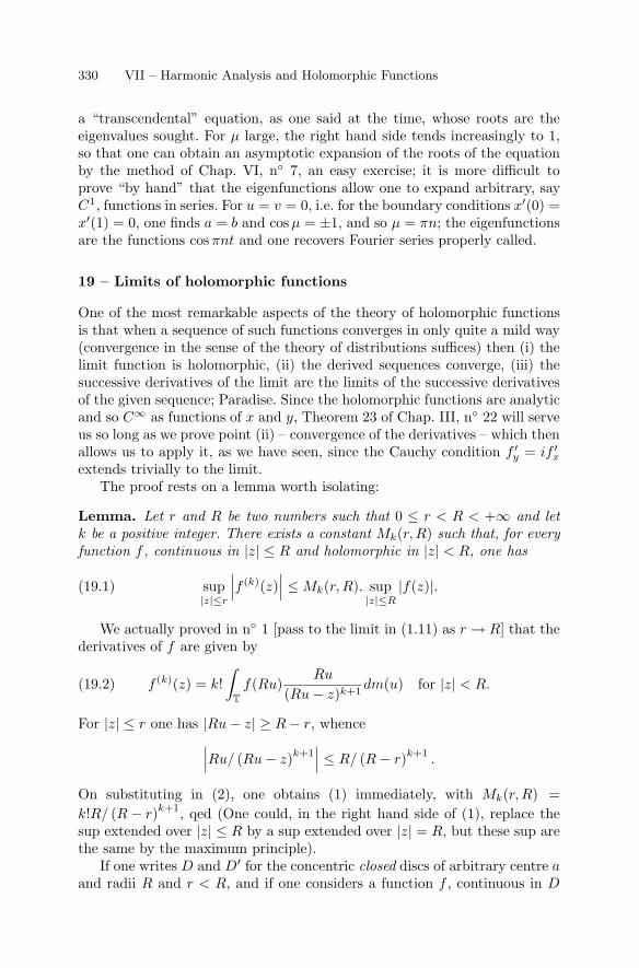
330 VII – Harmonic Analysis and Holomorphic Functions
a “transcendental” equation, as one said at the time, whose roots are theeigenvalues sought. For µ large, the right hand side tends increasingly to 1,so that one can obtain an asymptotic expansion of the roots of the equationby the method of Chap. VI, n◦ 7, an easy exercise; it is more difficult toprove “by hand” that the eigenfunctions allow one to expand arbitrary, sayC1, functions in series. For u = v = 0, i.e. for the boundary conditions x′(0) =x′(1) = 0, one finds a = b and cos µ = ±1, and so µ = πn; the eigenfunctionsare the functions cos πnt and one recovers Fourier series properly called.
19 – Limits of holomorphic functions
One of the most remarkable aspects of the theory of holomorphic functionsis that when a sequence of such functions converges in only quite a mild way(convergence in the sense of the theory of distributions suffices) then (i) thelimit function is holomorphic, (ii) the derived sequences converge, (iii) thesuccessive derivatives of the limit are the limits of the successive derivativesof the given sequence; Paradise. Since the holomorphic functions are analyticand so C∞ as functions of x and y, Theorem 23 of Chap. III, n◦ 22 will serveus so long as we prove point (ii) – convergence of the derivatives – which thenallows us to apply it, as we have seen, since the Cauchy condition f ′
y = if ′x
extends trivially to the limit.The proof rests on a lemma worth isolating:
Lemma. Let r and R be two numbers such that 0 ≤ r < R < +∞ and letk be a positive integer. There exists a constant Mk(r,R) such that, for everyfunction f , continuous in |z| ≤ R and holomorphic in |z| < R, one has
sup|z|≤r
∣∣∣f (k)(z)∣∣∣ ≤ Mk(r,R). sup
|z|≤R
|f(z)|.(19.1)
We actually proved in n◦ 1 [pass to the limit in (1.11) as r → R] that thederivatives of f are given by
f (k)(z) = k!∫
T
f(Ru)Ru
(Ru − z)k+1dm(u) for |z| < R.(19.2)
For |z| ≤ r one has |Ru − z| ≥ R − r, whence∣∣∣Ru/ (Ru − z)k+1∣∣∣ ≤ R/ (R − r)k+1
.
On substituting in (2), one obtains (1) immediately, with Mk(r,R) =k!R/ (R − r)k+1, qed (One could, in the right hand side of (1), replace thesup extended over |z| ≤ R by a sup extended over |z| = R, but these sup arethe same by the maximum principle).
If one writes D and D′ for the concentric closed discs of arbitrary centre aand radii R and r < R, and if one considers a function f , continuous in D
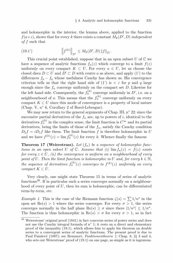
§ 4. Analytic and holomorphic functions 331
and holomorphic in the interior, the lemma above, applied to the functionf(a+z), shows that for every k there exists a constant Mk(D′, D) independentof f such that ∥∥∥f (k)
∥∥∥D′
≤ Mk(D′, D) ‖f‖D .(19.1’)
This crucial point established, suppose that in an open subset U of C wehave a sequence of analytic functions fn(z) which converge to a limit f(z)uniformly on every compact K ⊂ U . For every a ∈ U , let us choose theclosed discs D ⊂ U and D′ ⊂ D with centre a as above, and apply (1’) to thedifferences fp − fq whose usefulness Cauchy has shown us. His convergencecriterion tells us that the right hand side of (1’) is < ε for p and q largeenough since the fn converge uniformly on the compact set D. Likewise forthe left hand side. Consequently, the f
(k)n converge uniformly in D′, i.e. on a
neighbourhood of a. This means that the f(k)n converge uniformly on every
compact K ⊂ U since this mode of convergence is a property of local nature(Chap. V, n◦ 6, Corollary 2 of Borel-Lebesgue).
We may now return to the general arguments of Chap. III, n◦ 22: since thesuccessive partial derivatives of the fn are, up to powers of i, identical to thederivatives f
(k)n in the complex sense, the limit function is C∞ and its partial
derivatives, being the limits of those of the fn, satisfy the Cauchy conditionD2f = iD1f like them. The limit function f is therefore holomorphic in U
and we have f (k)(z) = lim f(k)n (z) for every k. Whence finally the famous
Theorem 17 (Weierstrass). Let (fn) be a sequence of holomorphic func-tions in an open subset U of C. Assume that (i) lim fn(z) = f(z) existsfor every z ∈ U , (ii) the convergence is uniform on a neighbourhood of everypoint of U . Then the limit function is holomorphic in U and, for every k ∈ N,the sequence of derivatives f
(k)n (z) converges to f (k)(z) uniformly on every
compact K ⊂ U .
Very clearly, one might state Theorem 15 in terms of series of analyticfunctions39. If in particular such a series converges normally on a neighbour-hood of every point of U , then its sum is holomorphic, can be differentiatedterm-by-term, etc.
Example 1. This is the case of the Riemann function ζ(s) =∑
1/ns in theopen set Re(s) > 1 where the series converges. For every σ > 1, the seriesconverges normally in the half plane Re(s) ≥ σ since there |1/ns| ≤ 1/nσ.The function is thus holomorphic in Re(s) > σ for every σ > 1, so in fact39 Weierstrass’ original proof (1841) in fact concerns series of power series and does
not use the Cauchy integral formula of n◦ 1; it rests on a direct and elementaryproof of the inequality (19.1), which allows him to apply his theorem on doubleseries to a convergent series of analytic functions. The present proof is due toPaul Painleve (1887); see Remmert, Funktionentheorie 1, Chap. 8, §§ 3 and 4,who sets out Weierstrass’ proof of (19.1) on one page, as simple as it is ingenious.
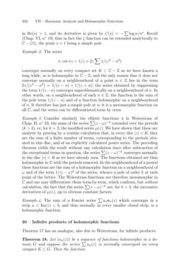
332 VII – Harmonic Analysis and Holomorphic Functions
in Re(s) > 1, and its derivative is given by ζ ′(s) = −∑ log n/ns. Recall(Chap. VI, n◦ 19) that in fact the ζ function can be extended analytically toC − {1}, the point s = 1 being a simple pole.
Example 2. The series
π. cot πz = 1/z + 2z∑
1/(z2 − n2)
converges normally on every compact set K ⊂ C − Z as we have known along while, so is holomorphic in C − Z; and the only reason that it does notconverge normally on a neighbourhood of a point n ∈ Z lies in the term2z/(z2 − n2) = 1/(z − n) + 1/(z + n): the series obtained by suppressingthe term 1/(z −n) converges unproblematically on a neighbourhood of n. Inother words, on a neighbourhood of each n ∈ Z, the function is the sum ofthe pole term 1/(z − n) and of a function holomorphic on a neighbourhoodof n. It therefore has just a simple pole at n; it is a meromorphic function onall C, and the series can be differentiated term by term.
Example 3. Consider similarly the elliptic functions a la Weierstrass ofChap. II, n◦ 23, the sums of the series
∑(z−ω)−k extended over the periods
(k > 3), or, for k = 2, the modified series ℘(z). We have shown that these areanalytic by proving by a routine calculation that, in every disc |z| < R, theyare the sum of a finite number of terms, corresponding to the periods situ-ated in this disc, and of an explicitly calculated power series. The precedingtheorem yields the result without any calculation since after subtraction ofthe exceptional terms in question, the series
∑(z −ω)−k converges normally
in the disc |z| < R as we have already seen. The functions obtained are thusholomorphic in C with the periods removed. In the neighbourhood of a periodthese functions are the sum of a holomorphic function on a neighbourhood ofω and of the term 1/(z − ω)k of the series, whence a pole of order k at eachpoint of the lattice. The Weierstrass functions are therefore meromorphic inC and one may differentiate them term-by-term, which confirms, but withoutcalculation, the fact that the series
∑(z−ω)−k are, for k > 3, the successive
derivatives of ℘(z), up to obvious constant factors.
Example 4. The sum of a Fourier series∑
anen(z) which converges in astrip a < Im(z) < b, and thus normally in every smaller closed strip, is aholomorphic function.
20 – Infinite products of holomorphic functions
Theorem 17 has an analogue, also due to Weierstrass, for infinite products:
Theorem 18. Let (un(z)) be a sequence of functions holomorphic in a do-main G and suppose the series
∑un(z) is normally convergent on every
compact K ⊂ G. Then the function
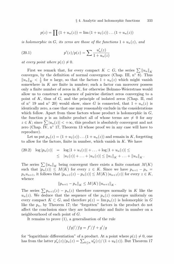
§ 4. Analytic and holomorphic functions 333
p(z) =∏
(1 + un(z)) = lim (1 + u1(z)) . . . (1 + un(z))
is holomorphic in G, its zeros are those of the functions 1 + un(z), and
p′(z)/p(z) =∑ u′
n(z)1 + un(z)
(20.1)
at every point where p(z) �= 0.
First we remark that, for every compact K ⊂ G, the series∑ ‖un‖K
converges, by the definition of normal convergence (Chap. III, n◦ 8). Thus‖un‖K < 1
2 for n large, so that the factors 1 + un(z) which might vanishsomewhere in K are finite in number; such a factor can moreover possessonly a finite number of zeros in K, for otherwise Bolzano-Weierstrass wouldallow us to construct a sequence of pairwise distinct zeros converging to apoint of K, thus of G, and the principle of isolated zeros (Chap. II, endof n◦ 19 and n◦ 20) would show, since G is connected, that 1 + un(z) isidentically zero, a case that one may reasonably exclude in the considerationswhich follow. Apart from these factors whose product is holomorphic in G,the function p is an infinite product all of whose terms are �= 0 for anyz ∈ K; since
∑ |un(z)| < +∞, this product is absolutely convergent and notzero (Chap. IV, n◦ 17, Theorem 13 whose proof we in any case will have toreproduce).
Let us put pn(z) = (1 + u1(z)) . . . (1 + un(z)) and remain in K, forgettingto allow for the factors, finite in number, which vanish in K. We have
log |pn(z)| = log |1 + u1(z)| + . . . + log |1 + un(z)| ≤(20.2)≤ |u1(z)| + . . . + |un(z)| ≤ ‖u1‖K + . . . + ‖un‖K .
The series∑ ‖un‖K being convergent there exists a finite constant M(K)
such that |pn(z)| ≤ M(K) for every z ∈ K. Since we have pn+1 − pn =pnun+1, it follows that |pn+1(z) − pn(z)| ≤ M(K) |un+1(z)| for every z ∈ K,whence
‖pn+1 − pn‖K ≤ M(K) ‖un+1‖K .
The series∑
pn+1(z) − pn(z) therefore converges normally in K like theun(z). We deduce that the sequence of the pn(z) converges uniformly onevery compact K ⊂ G, and therefore p(z) = lim pn(z) is holomorphic in Glike the pn, by Theorem 17; the “forgotten” factors in the product do notaffect the conclusion since they are holomorphic and finite in number on aneighbourhood of each point of G.
It remains to prove (1), a generalisation of the rule
(fg)′/fg = f ′/f + g′/g
for “logarithmic differentiation” of a product. At a point where p(z) �= 0, onehas from the latter p′n(z)/pn(z) =
∑k≤n u′
k(z)/ (1 + uk(z)). But Theorem 17
334 VII – Harmonic Analysis and Holomorphic Functions
assures us that lim p′n(z) = p′(z), and since pn(z) tends to p(z) �= 0, onededuces that p′(z)/p(z) is the limit of the partial sums of the series (1).
In fact, the latter converges normally on every compact K ⊂ G. It suffices,as always, to show this on a neighbourhood of every a ∈ G. To do this,consider a compact disc D : |z−a| ≤ R contained in G and a disc D′ : |z−a| ≤r < R contained in the interior of the first. The lemma of n◦ 19 provides anupper estimate ‖u′
n‖D′ ≤ M ‖un‖D with a constant M independent of n.On the other hand ‖un‖D < 1
2 for n large, as we have seen above, andthus ‖1 + un‖D > 1
2 . The uniform norm on D′ of the general term of theseries (1) is therefore majorised for n large by 2M ‖un‖D, whence the normalconvergence of (1) in D′, and so on every compact K ⊂ U , qed.
Example 1. Consider (Chap. IV, n◦ 20) Euler’s formula
P (z) =∏n≥1
(1 − zn)−1 =∑n≥0
p(n)zn
which appears in the theory of partitions. Theorem 18 shows that the product∏(1 − zn) is holomorphic in the disc D : |z| < 1 and never vanishes; the left
hand side is therefore also holomorphic in D, whence the existence of anexpansion in power series in D. Since we have p(n) ≥ 1 (this is the least onecould say . . .), the radius of convergence is equal to 1.
The function P (z) is an example of a curious phenomenon: it is not possi-ble to “extend the function P analytically” outside D: if an analytic functiondefined in a domain G ⊃ D coincides with P in D, then G = D. One mayunderstand this by observing that P (z) seems not to tend to any limit whenz tends to any root of unity, since then infinitely many factors of the productbecome infinite, but this is not a proof . . .
Example 2. Let q be a constant complex such that |q| < 1 and let us considerthe infinite product
f(z) =∏
(1 + qnz) ,(20.3)
where the product is extended over all n ≥ 1. Since∑ |qn| < +∞, Weier-
strass’ theorem applies, the result being an entire function of z. It is clearthat f(z) = (1 + qz)f(qz), so that the power series f(z) =
∑anzn which
represents f in the whole plane satisfies∑anzn = (1 + qz)
∑anqnzn;
one deduces that an = qnan + qnan−1, i.e. that
(1 − qn) an = qnan−1.
Since a0 = f(0) = 1, it follows that
§ 4. Analytic and holomorphic functions 335
an = q1+2+...+n/(1 − q) . . . (1 − qn) ,
whence the identity
∞∏n=1
(1 + qnz) = 1 +∞∑
n=1
qn(n+1)/2
(1 − q) . . . (1 − qn)zn (|q| < 1, z ∈ C).(20.4)
Exercise: show that∞∏
n=0
(1 + qnz)−1 =∞∑
n=0
(−1)nzn
(1 − q) . . . (1 − qn)(20.5)
for |q| < 1, |z| < 1. What happens for |z| > 1?
Example 3. Consider the infinite product
f(z) = z∏(
1 − z2/n2)
(20.6)
extended over n ≥ 1. It satisfies the hypotheses of the theorem, with G = C,so represents an entire function having simple zeros at the n ∈ Z and isnonzero elsewhere. Theorem 18 shows that
f ′(z)/f(z) = 1/z +∑
2z/(z2 − n2
)= π. cot πz = (sin πz)′/ sin πz.(20.7)
In the connected open set C−Z where it is defined, the holomorphic functionf(z)/ sin πz thus has derivative zero, so is constant; since f(z)/z and sinπz/ztend respectively to 1 and π when z tends to 0, this constant is equal to 1/π.Whence
sin πz = πz∏(
1 − z2/n2).(20.8)
This proof of Euler’s infinite product manifests the fantastical characterof his considerations on “algebraic equations of infinite degree” (Chap. II, endof n◦ 21). As we have said, the infinite product (6) is an entire function whoseonly zeros are the n ∈ Z; on a neighbourhood of such a point, f(z) is theproduct of 1−z/n by an infinite product which no longer vanishes at n, so thatthe n ∈ Z are simple zeros of f . Since it is clear that z = n is likewise a simplezero of the function sinπz (obvious for n = 0, so for any n by periodicity),one deduces that sin πz = g(z)f(z) where g is an everywhere holomorphicfunction (so analytic) having no zero in C. For such a function, the quotientg′(z)/g(z) is again an entire function, so an everywhere convergent powerseries, so has in C a primitive h(z) such that h′(z) = g′(z)/g(z) as we know(Chap. II, n◦ 19). It follows that
(ge−h)′
= g′e−h − gh′e−h = 0,
336 VII – Harmonic Analysis and Holomorphic Functions
so that g(z) = ceh(z) where c is a constant that one may assume equal to 1 byincorporating a suitable constant into h. Euler’s argument, corrected, thusproves the existence of a relation of the form
sin πz = eh(z)z∏(
1 − z2/n2)
(20.9)
with an entire function h about which the preceding argument provides noinformation whatsoever . . .
In fact, Weierstrass invented, and his successors refined, a whole theorythat allows one to represent any entire function f by an infinite product thatexhibits its zeros, but this is much less simple than Euler’s ideas. The firstidea is to order the zeros an of f in a sequence40 such that |an| ≤ |an+1|,then to consider the infinite product
∏(1 − z/an). This then has exactly
the same zeros as f , with the same orders of multiplicity, whence f(z) =g(z)∏
(1 − z/an) where g is an entire function without zeros, so of the formeh(z). This is Euler’s marvellous argument (except that he forgot the factorg).
But first one should verify the convergence of the infinite product! Thoughobvious in the case of the function sinus when one groups the symmetricfactors, it can be perfectly false in the case of an arbitrary entire function41.
Weierstrass’ idea is now to multiply each factor 1 − z/an by as simple afunction as possible, vanishing nowhere so as not to add parasitic zeros to theproduct, and making the infinite product convergent. This technique is veryshrewd. First, it is clear that, for z given, z/an tends to 0, so is in modulus< 1 for n large. Consider, generally, 1 − z for |z| < 1. Then
1 − z = exp(−z − z2/2 − z3/3 − . . .
)[Chap. IV, (13.12)], whence, for every p,
1 − z = exp (z + . . . + zp/p)−1 exp[−zp+1/(p + 1) − . . .
].
Consider the functions
Ep(z) = (1 − z) exp (z + . . . + zp/p) = exp[−zp+1/(p + 1) − . . .
].(20.10)
The factor exp (z + . . . + zp/p) never vanishes and tends to 1 when z tendsto 0, as does Ep(z). Let us prove that
40 The set of zeros is countable, for, by the principle of isolated zeros, there can beonly finitely many in the disc |z| < p for any p ∈ N. In what follows, we assumethat each zero appears as many times among the an as its order of multiplicity.
41 Consider the function sin(πz2). Its zeros are the z such that z2 ∈ Z, so the
points of the form n1/2 or in1/2, and the infinite product is divergent like theseries∑
1/|n|1/2.
§ 4. Analytic and holomorphic functions 337
|1 − Ep(z)| ≤ |z|p+1 for |z| ≤ 1.(20.11)
The function 1−Ep(z) vanishes at the origin and is holomorphic in all C; itsderivative
−E′p(z) = zp exp (z + . . . + zp/p) = zp
∑n
(z + . . . + zp/p)[n](20.12)
(exercise!) is an everywhere convergent power series with all its coefficientspositive (Theorem 17) and whose term of lowest degree is zp; that of 1 −Ep(z) therefore starts with a term in zp+1. Schwarz’ lemma now shows that|1 − Ep(z)| ≤ M |z|p+1, where M is the maximum of |1 − Ep(z)| on the circle|z| = 1; but since the coefficients of the power series of 1 − Ep(z) are, likethose of its derivative, all positive, its maximum on |z| = 1 is attained forz = 1 and so is equal to 1 by (10); whence (11), thanks to Remmert.
This point completed, let us return to the entire function f(z) and to itszeros an. The function Ep (z/an) = (1 − z/an) exp(. . .) has a simple zero atan and is �= 0 elsewhere. We may therefore try to compare f(z) with theinfinite product
h(z) =∏
Epn(1 − z/an)(20.13)
where the pn are chosen to make the product absolutely convergent. Since itcan be written as
∏[1 + un(z)] with
|un(z)| ≤ |z/an|pn+1
by (11), and since, for every compact K ⊂ C, we have |z/an| ≤ 12 for every
z ∈ K if n is large enough (the |an| increase indefinitely since the zeros ofan entire function are isolated in C), we may always choose the pn to makethe series
∑un(z) normally convergent on every compact; at the worst, we
choose pn = n − 1 for every n.This done, we have, as in the case of the function sin πz, a relation
f(z) = eg(z)∏
Epn(1 − z/an)(20.14)
with an entire function g(z) about which, a priori, we know nothing.It goes without saying that the choice pn = n − 1 is not always the best
possible, as shown by the case of the function sinus, and that, moreover,il would be useful to determine the function g(z) more precisely. There aretheorems that apply to functions that do not increase too fast at infinity. Toenter into this difficult subject which has interested (too) many specialistswould no doubt exceed the capacity of most of our readers, and, even morecertainly, of the author.
Example 4 (infinite product for the Gamma function). Consider Euler’s func-tion
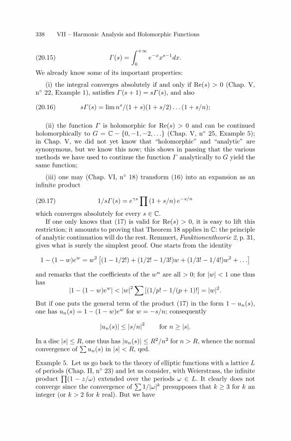
338 VII – Harmonic Analysis and Holomorphic Functions
Γ (s) =∫ +∞
0
e−xxs−1dx.(20.15)
We already know some of its important properties:
(i) the integral converges absolutely if and only if Re(s) > 0 (Chap. V,n◦ 22, Example 1), satisfies Γ (s + 1) = sΓ (s), and also
sΓ (s) = limns/(1 + s)(1 + s/2) . . . (1 + s/n);(20.16)
(ii) the function Γ is holomorphic for Re(s) > 0 and can be continuedholomorphically to G = C − {0,−1,−2, . . .} (Chap. V, n◦ 25, Example 5);in Chap. V, we did not yet know that “holomorphic” and “analytic” aresynonymous, but we know this now; this shows in passing that the variousmethods we have used to continue the function Γ analytically to G yield thesame function;
(iii) one may (Chap. VI, n◦ 18) transform (16) into an expansion as aninfinite product
1/sΓ (s) = eγs∏
(1 + s/n) e−s/n(20.17)
which converges absolutely for every s ∈ C.If one only knows that (17) is valid for Re(s) > 0, it is easy to lift this
restriction; it amounts to proving that Theorem 18 applies in C: the principleof analytic continuation will do the rest. Remmert, Funktionentheorie 2, p. 31,gives what is surely the simplest proof. One starts from the identity
1 − (1 − w)ew = w2[(1 − 1/2!) + (1/2! − 1/3!)w + (1/3! − 1/4!)w2 + . . .
]and remarks that the coefficients of the wn are all > 0; for |w| < 1 one thushas
|1 − (1 − w)ew| < |w|2∑
[(1/p! − 1/(p + 1)!] = |w|2.But if one puts the general term of the product (17) in the form 1 − un(s),one has un(s) = 1 − (1 − w)ew for w = −s/n; consequently
|un(s)| ≤ |s/n|2 for n ≥ |s|.
In a disc |s| ≤ R, one thus has |un(s)| ≤ R2/n2 for n > R, whence the normalconvergence of
∑un(s) in |s| < R, qed.
Example 5. Let us go back to the theory of elliptic functions with a lattice Lof periods (Chap. II, n◦ 23) and let us consider, with Weierstrass, the infiniteproduct
∏(1 − z/ω) extended over the periods ω ∈ L. It clearly does not
converge since the convergence of∑
1/|ω|k presupposes that k ≥ 3 for k aninteger (or k > 2 for k real). But we have
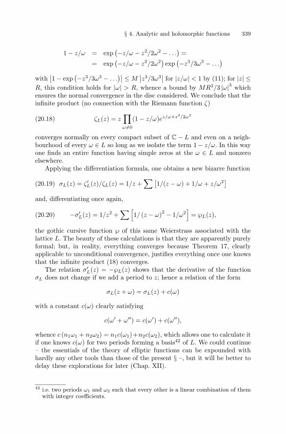
§ 4. Analytic and holomorphic functions 339
1 − z/ω = exp(−z/ω − z2/2ω2 − . . .
)=
= exp(−z/ω − z2/2ω2
)exp(−z3/3ω3 − . . .
)with∣∣1 − exp
(−z3/3ω3 − . . .)∣∣ ≤ M
∣∣z3/3ω3∣∣ for |z/ω| < 1 by (11); for |z| ≤
R, this condition holds for |ω| > R, whence a bound by MR3/3 |ω|3 whichensures the normal convergence in the disc considered. We conclude that theinfinite product (no connection with the Riemann function ζ)
ζL(z) = z∏ω �=0
(1 − z/ω)ez/ω+z2/2ω2(20.18)
converges normally on every compact subset of C − L and even on a neigh-bourhood of every ω ∈ L so long as we isolate the term 1− z/ω. In this wayone finds an entire function having simple zeros at the ω ∈ L and nonzeroelsewhere.
Applying the differentiation formula, one obtains a new bizarre function
σL(z) = ζ ′L(z)/ζL(z) = 1/z +∑[
1/(z − ω) + 1/ω + z/ω2]
(20.19)
and, differentiating once again,
−σ′L(z) = 1/z2 +
∑[1/ (z − ω)2 − 1/ω2
]= ℘L(z),(20.20)
the gothic cursive function ℘ of this same Weierstrass associated with thelattice L. The beauty of these calculations is that they are apparently purelyformal; but, in reality, everything converges because Theorem 17, clearlyapplicable to unconditional convergence, justifies everything once one knowsthat the infinite product (18) converges.
The relation σ′L(z) = −℘L(z) shows that the derivative of the function
σL does not change if we add a period to z; hence a relation of the form
σL(z + ω) = σL(z) + c(ω)
with a constant c(ω) clearly satisfying
c(ω′ + ω′′) = c(ω′) + c(ω′′),
whence c (n1ω1 + n2ω2) = n1c(ω1)+n2c(ω2), which allows one to calculate itif one knows c(ω) for two periods forming a basis42 of L. We could continue– the essentials of the theory of elliptic functions can be expounded withhardly any other tools than those of the present § –, but it will be better todelay these explorations for later (Chap. XII).
42 i.e. two periods ω1 and ω2 such that every other is a linear combination of themwith integer coefficients.
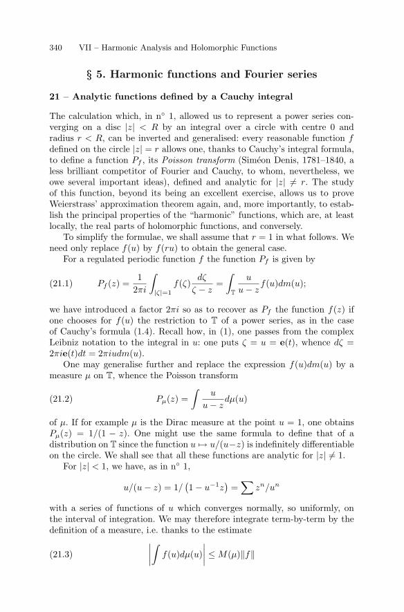
340 VII – Harmonic Analysis and Holomorphic Functions
§ 5. Harmonic functions and Fourier series
21 – Analytic functions defined by a Cauchy integral
The calculation which, in n◦ 1, allowed us to represent a power series con-verging on a disc |z| < R by an integral over a circle with centre 0 andradius r < R, can be inverted and generalised: every reasonable function fdefined on the circle |z| = r allows one, thanks to Cauchy’s integral formula,to define a function Pf , its Poisson transform (Simeon Denis, 1781–1840, aless brilliant competitor of Fourier and Cauchy, to whom, nevertheless, weowe several important ideas), defined and analytic for |z| �= r. The studyof this function, beyond its being an excellent exercise, allows us to proveWeierstrass’ approximation theorem again, and, more importantly, to estab-lish the principal properties of the “harmonic” functions, which are, at leastlocally, the real parts of holomorphic functions, and conversely.
To simplify the formulae, we shall assume that r = 1 in what follows. Weneed only replace f(u) by f(ru) to obtain the general case.
For a regulated periodic function f the function Pf is given by
Pf (z) =1
2πi
∫|ζ|=1
f(ζ)dζ
ζ − z=∫
T
u
u − zf(u)dm(u);(21.1)
we have introduced a factor 2πi so as to recover as Pf the function f(z) ifone chooses for f(u) the restriction to T of a power series, as in the caseof Cauchy’s formula (1.4). Recall how, in (1), one passes from the complexLeibniz notation to the integral in u: one puts ζ = u = e(t), whence dζ =2πie(t)dt = 2πiudm(u).
One may generalise further and replace the expression f(u)dm(u) by ameasure µ on T, whence the Poisson transform
Pµ(z) =∫
u
u − zdµ(u)(21.2)
of µ. If for example µ is the Dirac measure at the point u = 1, one obtainsPµ(z) = 1/(1 − z). One might use the same formula to define that of adistribution on T since the function u → u/(u−z) is indefinitely differentiableon the circle. We shall see that all these functions are analytic for |z| �= 1.
For |z| < 1, we have, as in n◦ 1,
u/(u − z) = 1/(1 − u−1z
)=∑
zn/un
with a series of functions of u which converges normally, so uniformly, onthe interval of integration. We may therefore integrate term-by-term by thedefinition of a measure, i.e. thanks to the estimate∣∣∣∣
∫f(u)dµ(u)
∣∣∣∣ ≤ M(µ)‖f‖(21.3)
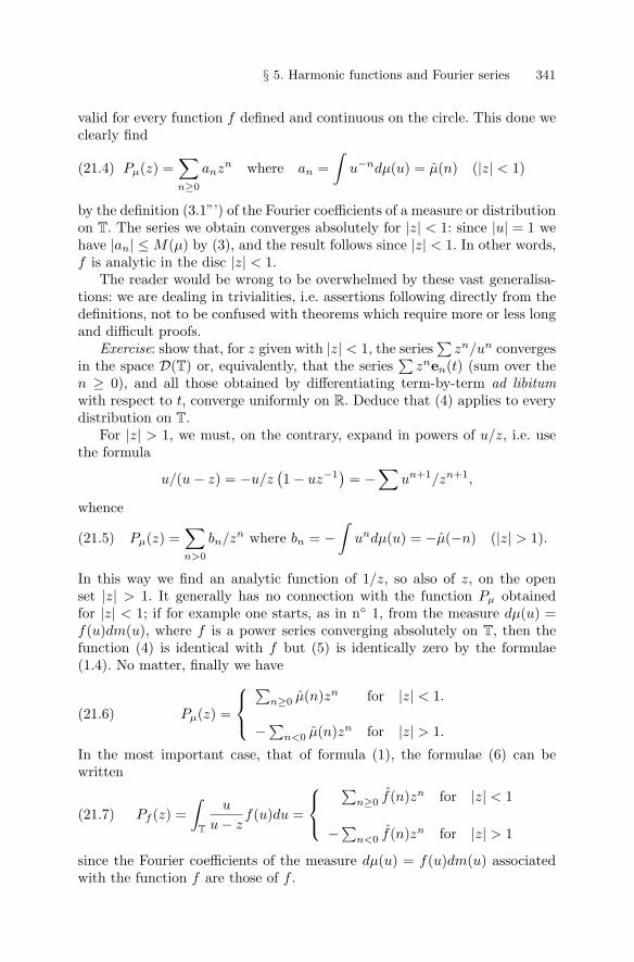
§ 5. Harmonic functions and Fourier series 341
valid for every function f defined and continuous on the circle. This done weclearly find
Pµ(z) =∑n≥0
anzn where an =∫
u−ndµ(u) = µ(n) (|z| < 1)(21.4)
by the definition (3.1”’) of the Fourier coefficients of a measure or distributionon T. The series we obtain converges absolutely for |z| < 1: since |u| = 1 wehave |an| ≤ M(µ) by (3), and the result follows since |z| < 1. In other words,f is analytic in the disc |z| < 1.
The reader would be wrong to be overwhelmed by these vast generalisa-tions: we are dealing in trivialities, i.e. assertions following directly from thedefinitions, not to be confused with theorems which require more or less longand difficult proofs.
Exercise: show that, for z given with |z| < 1, the series∑
zn/un convergesin the space D(T) or, equivalently, that the series
∑znen(t) (sum over the
n ≥ 0), and all those obtained by differentiating term-by-term ad libitumwith respect to t, converge uniformly on R. Deduce that (4) applies to everydistribution on T.
For |z| > 1, we must, on the contrary, expand in powers of u/z, i.e. usethe formula
u/(u − z) = −u/z(1 − uz−1
)= −∑
un+1/zn+1,
whence
Pµ(z) =∑n>0
bn/zn where bn = −∫
undµ(u) = −µ(−n) (|z| > 1).(21.5)
In this way we find an analytic function of 1/z, so also of z, on the openset |z| > 1. It generally has no connection with the function Pµ obtainedfor |z| < 1; if for example one starts, as in n◦ 1, from the measure dµ(u) =f(u)dm(u), where f is a power series converging absolutely on T, then thefunction (4) is identical with f but (5) is identically zero by the formulae(1.4). No matter, finally we have
Pµ(z) =
⎧⎨⎩∑
n≥0 µ(n)zn for |z| < 1.
−∑n<0 µ(n)zn for |z| > 1.(21.6)
In the most important case, that of formula (1), the formulae (6) can bewritten
Pf (z) =∫
T
u
u − zf(u)du =
⎧⎨⎩∑
n≥0 f(n)zn for |z| < 1
−∑n<0 f(n)zn for |z| > 1(21.7)
since the Fourier coefficients of the measure dµ(u) = f(u)dm(u) associatedwith the function f are those of f .
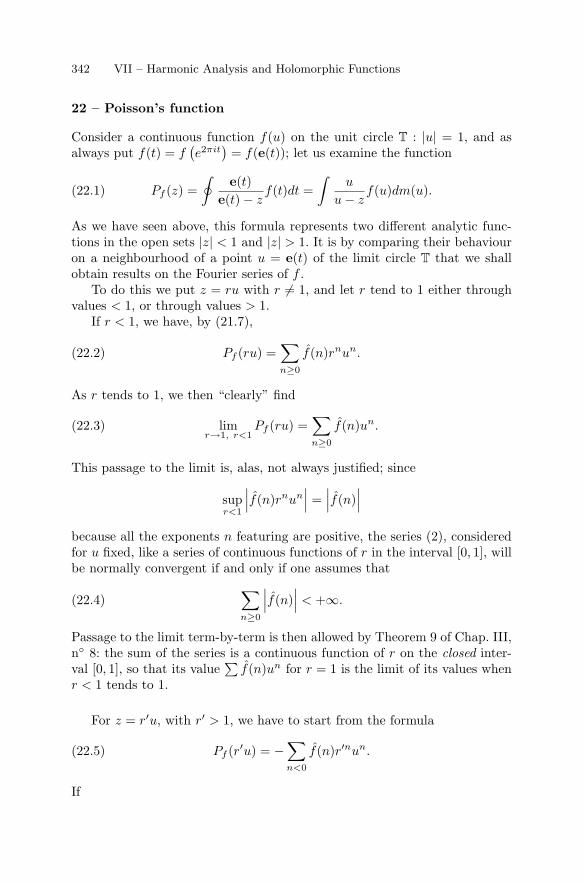
342 VII – Harmonic Analysis and Holomorphic Functions
22 – Poisson’s function
Consider a continuous function f(u) on the unit circle T : |u| = 1, and asalways put f(t) = f
(e2πit)
= f(e(t)); let us examine the function
Pf (z) =∮
e(t)e(t) − z
f(t)dt =∫
u
u − zf(u)dm(u).(22.1)
As we have seen above, this formula represents two different analytic func-tions in the open sets |z| < 1 and |z| > 1. It is by comparing their behaviouron a neighbourhood of a point u = e(t) of the limit circle T that we shallobtain results on the Fourier series of f .
To do this we put z = ru with r �= 1, and let r tend to 1 either throughvalues < 1, or through values > 1.
If r < 1, we have, by (21.7),
Pf (ru) =∑n≥0
f(n)rnun.(22.2)
As r tends to 1, we then “clearly” find
limr→1, r<1
Pf (ru) =∑n≥0
f(n)un.(22.3)
This passage to the limit is, alas, not always justified; since
supr<1
∣∣∣f(n)rnun∣∣∣ = ∣∣∣f(n)
∣∣∣because all the exponents n featuring are positive, the series (2), consideredfor u fixed, like a series of continuous functions of r in the interval [0, 1], willbe normally convergent if and only if one assumes that∑
n≥0
∣∣∣f(n)∣∣∣ < +∞.(22.4)
Passage to the limit term-by-term is then allowed by Theorem 9 of Chap. III,n◦ 8: the sum of the series is a continuous function of r on the closed inter-val [0, 1], so that its value
∑f(n)un for r = 1 is the limit of its values when
r < 1 tends to 1.
For z = r′u, with r′ > 1, we have to start from the formula
Pf (r′u) = −∑n<0
f(n)r′nun.(22.5)
If
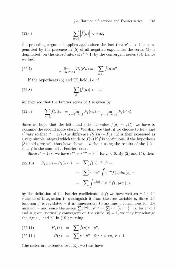
§ 5. Harmonic functions and Fourier series 343
∑n<0
∣∣∣f(n)∣∣∣ < +∞,(22.6)
the preceding argument applies again since the fact that r′ is > 1 is com-pensated by the presence in (5) of all negative exponents: the series (5) isdominated, on the closed interval r′ ≥ 1, by the convergent series (6). Hencewe find
limr′→1, r′>1
Pf (r′u) = −∑n<0
f(n)un.(22.7)
If the hypotheses (5) and (7) hold, i.e. if∑Z
|f(n)| < +∞,(22.8)
we then see that the Fourier series of f is given by∑n∈Z
f(n)un = limr→1, r<1
Pf (ru) − limr′→1, r′>1
Pf (r′u).(22.9)
Since we hope that the left hand side has value f(u) = f(t), we have toexamine the second more closely. We shall see that, if we choose to let r andr′ vary so that r′ = 1/r, the difference Pf (ru)−Pf (r′u) is then expressed asa very simple integral which tends to f(u) if f is continuous; if the hypothesis(8) holds, we will thus have shown – without using the results of the § 2 –that f is the sum of its Fourier series.
Since r′ = 1/r, we have r′n = r−n = r|n| for n < 0. By (2) and (5), then
Pf (ru) − Pf (u/r) =∑
f(n)r|n|un =(22.10)
=∑
r|n|un
∫v−nf(v)dm(v) =
=∑∫
r|n|unv−nf(v)dm(v)
by the definition of the Fourier coefficients of f ; we have written v for thevariable of integration to distinguish it from the free variable u. Since thefunction f is regulated – it is unnecessary to assume it continuous for themoment – and since the series
∑r|n|unv−n =
∑r|n|(uv−1)n is, for r < 1
and u given, normally convergent on the circle |v| = 1, we may interchangethe signs
∫and∑
in (10); putting
Hf (z) =∑
f(n)r|n|un,(22.11)
P (z) =∑
r|n|un for z = ru, r < 1,(22.11’)
(the series are extended over Z), we thus have
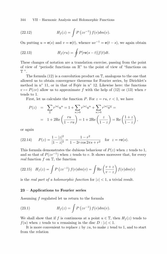
344 VII – Harmonic Analysis and Holomorphic Functions
Hf (z) =∫
P(zv−1)f(v)dm(v).(22.12)
On putting u = e(s) and v = e(t), whence uv−1 = e(t − s), we again obtain
Hf (ru) =∮
P [re(s − t)]f(t)dt.(22.13)
These changes of notation are a translation exercise, passing from the pointof view of “periodic functions on R” to the point of view of “functions onT ”.
The formula (12) is a convolution product on T, analogous to the one thatallowed us to obtain convergence theorems for Fourier series, by Dirichlet’smethod in n◦ 11, or in that of Fejer in n◦ 12. Likewise here: the functionsv → P (zv) allow us to approximate f with the help of (12) or (13) when rtends to 1.
First, let us calculate the function P . For z = ru, r < 1, we have
P (z) =∑
Z
r|n|un = 1 +∑n>0
r|n|un +∑n>0
r|n|un =
= 1 + 2Re(
ru
1 − ru
)= 1 + 2Re
(z
1 − z
)= Re(
1 + z
1 − z
),
or again
P (z) =1 − |z|2|1 − z|2 =
1 − r2
1 − 2r cos 2πs + r2for z = re(s).(22.14)
This formula demonstrates the dubious behaviour of P (z) when z tends to 1,and so that of P (zv−1) when z tends to v. It shows moreover that, for everyreal function f on T, the function
Hf (z) =∫
P(zv−1)f(v)dm(v) =
∫Re(
v + z
v − z
)f(v)dm(v)(22.15)
is the real part of a holomorphic function for |z| < 1, a trivial result.
23 – Applications to Fourier series
Assuming f regulated let us return to the formula
Hf (z) =∫
P(zv−1)f(v)dm(v).(23.1)
We shall show that if f is continuous at a point u ∈ T, then Hf (z) tends tof(u) when z tends to u remaining in the disc D : |z| < 1.
It is more convenient to replace z by zu, to make z tend to 1, and to startfrom the relation
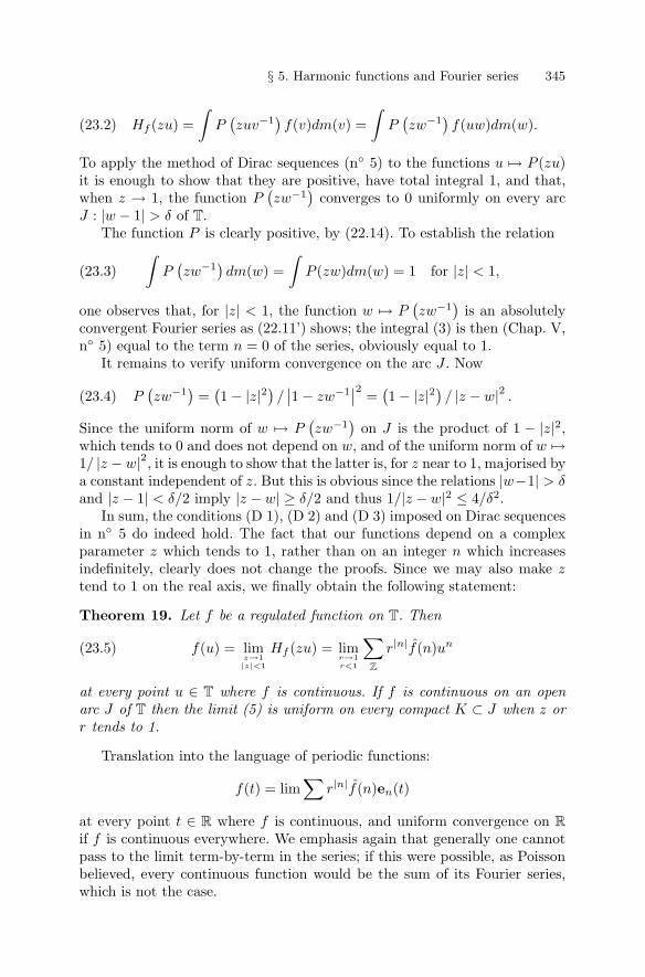
§ 5. Harmonic functions and Fourier series 345
Hf (zu) =∫
P(zuv−1)f(v)dm(v) =
∫P(zw−1)f(uw)dm(w).(23.2)
To apply the method of Dirac sequences (n◦ 5) to the functions u → P (zu)it is enough to show that they are positive, have total integral 1, and that,when z → 1, the function P
(zw−1)
converges to 0 uniformly on every arcJ : |w − 1| > δ of T.
The function P is clearly positive, by (22.14). To establish the relation∫P(zw−1)dm(w) =
∫P (zw)dm(w) = 1 for |z| < 1,(23.3)
one observes that, for |z| < 1, the function w → P(zw−1)
is an absolutelyconvergent Fourier series as (22.11’) shows; the integral (3) is then (Chap. V,n◦ 5) equal to the term n = 0 of the series, obviously equal to 1.
It remains to verify uniform convergence on the arc J . Now
P(zw−1)
=(1 − |z|2) / ∣∣1 − zw−1
∣∣2 =(1 − |z|2) / |z − w|2 .(23.4)
Since the uniform norm of w → P(zw−1)
on J is the product of 1 − |z|2,which tends to 0 and does not depend on w, and of the uniform norm of w →1/ |z − w|2, it is enough to show that the latter is, for z near to 1, majorised bya constant independent of z. But this is obvious since the relations |w−1| > δand |z − 1| < δ/2 imply |z − w| ≥ δ/2 and thus 1/|z − w|2 ≤ 4/δ2.
In sum, the conditions (D 1), (D 2) and (D 3) imposed on Dirac sequencesin n◦ 5 do indeed hold. The fact that our functions depend on a complexparameter z which tends to 1, rather than on an integer n which increasesindefinitely, clearly does not change the proofs. Since we may also make ztend to 1 on the real axis, we finally obtain the following statement:
Theorem 19. Let f be a regulated function on T. Then
f(u) = limz→1|z|<1
Hf (zu) = limr→1r<1
∑Z
r|n|f(n)un(23.5)
at every point u ∈ T where f is continuous. If f is continuous on an openarc J of T then the limit (5) is uniform on every compact K ⊂ J when z orr tends to 1.
Translation into the language of periodic functions:
f(t) = lim∑
r|n|f(n)en(t)
at every point t ∈ R where f is continuous, and uniform convergence on Rif f is continuous everywhere. We emphasis again that generally one cannotpass to the limit term-by-term in the series; if this were possible, as Poissonbelieved, every continuous function would be the sum of its Fourier series,which is not the case.
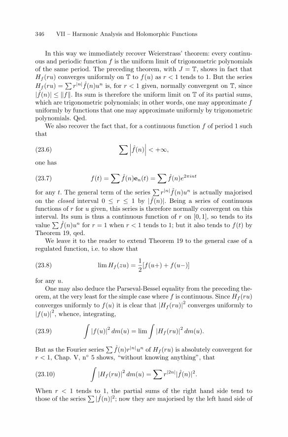
346 VII – Harmonic Analysis and Holomorphic Functions
In this way we immediately recover Weierstrass’ theorem: every continu-ous and periodic function f is the uniform limit of trigonometric polynomialsof the same period. The preceding theorem, with J = T, shows in fact thatHf (ru) converges uniformly on T to f(u) as r < 1 tends to 1. But the seriesHf (ru) =
∑r|n|f(n)un is, for r < 1 given, normally convergent on T, since
|f(n)| ≤ ‖f‖. Its sum is therefore the uniform limit on T of its partial sums,which are trigonometric polynomials; in other words, one may approximate funiformly by functions that one may approximate uniformly by trigonometricpolynomials. Qed.
We also recover the fact that, for a continuous function f of period 1 suchthat ∑∣∣∣f(n)
∣∣∣ < +∞,(23.6)
one has
f(t) =∑
f(n)en(t) =∑
f(n)e2πint(23.7)
for any t. The general term of the series∑
r|n|f(n)un is actually majorisedon the closed interval 0 ≤ r ≤ 1 by |f(n)|. Being a series of continuousfunctions of r for u given, this series is therefore normally convergent on thisinterval. Its sum is thus a continuous function of r on [0, 1], so tends to itsvalue∑
f(n)un for r = 1 when r < 1 tends to 1; but it also tends to f(t) byTheorem 19, qed.
We leave it to the reader to extend Theorem 19 to the general case of aregulated function, i.e. to show that
limHf (zu) =12[f(u+) + f(u−)](23.8)
for any u.One may also deduce the Parseval-Bessel equality from the preceding the-
orem, at the very least for the simple case where f is continuous. Since Hf (ru)converges uniformly to f(u) it is clear that |Hf (ru)|2 converges uniformly to|f(u)|2, whence, integrating,∫
|f(u)|2 dm(u) = lim∫
|Hf (ru)|2 dm(u).(23.9)
But as the Fourier series∑
f(n)r|n|un of Hf (ru) is absolutely convergent forr < 1, Chap. V, n◦ 5 shows, “without knowing anything”, that∫
|Hf (ru)|2 dm(u) =∑
r|2n||f(n)|2.(23.10)
When r < 1 tends to 1, the partial sums of the right hand side tend tothose of the series
∑ |f(n)|2; now they are majorised by the left hand side of
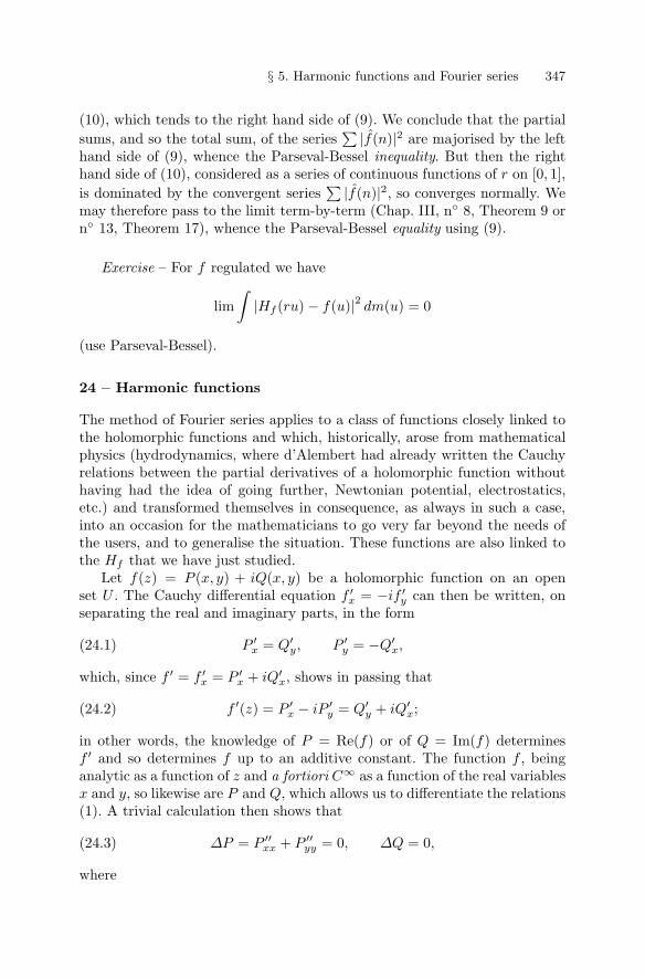
§ 5. Harmonic functions and Fourier series 347
(10), which tends to the right hand side of (9). We conclude that the partialsums, and so the total sum, of the series
∑ |f(n)|2 are majorised by the lefthand side of (9), whence the Parseval-Bessel inequality. But then the righthand side of (10), considered as a series of continuous functions of r on [0, 1],is dominated by the convergent series
∑ |f(n)|2, so converges normally. Wemay therefore pass to the limit term-by-term (Chap. III, n◦ 8, Theorem 9 orn◦ 13, Theorem 17), whence the Parseval-Bessel equality using (9).
Exercise – For f regulated we have
lim∫
|Hf (ru) − f(u)|2 dm(u) = 0
(use Parseval-Bessel).
24 – Harmonic functions
The method of Fourier series applies to a class of functions closely linked tothe holomorphic functions and which, historically, arose from mathematicalphysics (hydrodynamics, where d’Alembert had already written the Cauchyrelations between the partial derivatives of a holomorphic function withouthaving had the idea of going further, Newtonian potential, electrostatics,etc.) and transformed themselves in consequence, as always in such a case,into an occasion for the mathematicians to go very far beyond the needs ofthe users, and to generalise the situation. These functions are also linked tothe Hf that we have just studied.
Let f(z) = P (x, y) + iQ(x, y) be a holomorphic function on an openset U . The Cauchy differential equation f ′
x = −if ′y can then be written, on
separating the real and imaginary parts, in the form
P ′x = Q′
y, P ′y = −Q′
x,(24.1)
which, since f ′ = f ′x = P ′
x + iQ′x, shows in passing that
f ′(z) = P ′x − iP ′
y = Q′y + iQ′
x;(24.2)
in other words, the knowledge of P = Re(f) or of Q = Im(f) determinesf ′ and so determines f up to an additive constant. The function f , beinganalytic as a function of z and a fortiori C∞ as a function of the real variablesx and y, so likewise are P and Q, which allows us to differentiate the relations(1). A trivial calculation then shows that
∆P = P ′′xx + P ′′
yy = 0, ∆Q = 0,(24.3)
where
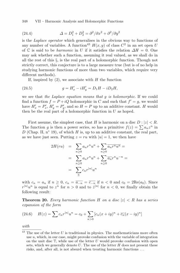
348 VII – Harmonic Analysis and Holomorphic Functions
∆ = D21 + D2
2 = ∂2/∂x2 + ∂2/∂y2(24.4)
is the Laplace operator which generalises in the obvious way to functions ofany number of variables. A function43 H(x, y) of class C2 in an set open Uof C is said to be harmonic in U if it satisfies the relation ∆H = 0. Onemay ask whether such a function, assuming it real valued, as we shall do inall the rest of this §, is the real part of a holomorphic function. Though notstrictly correct, this conjecture is to a large measure true (but is of no help instudying harmonic functions of more than two variables, which require verydifferent methods).
If, inspired by (2), we associate with H the function
g = H ′x − iH ′
y = D1H − iD2H,(24.5)
we see that the Laplace equation means that g is holomorphic. If we couldfind a function f = P + iQ holomorphic in C and such that f ′ = g, we wouldhave H ′
x = P ′x, H ′
y = P ′y, and so H = P up to an additive constant. H would
then be the real part of a holomorphic function in U as hoped.
First assume, the simplest case, that H is harmonic on a disc D : |z| < R.The function g is then a power series, so has a primitive f(z) =
∑anzn in
D (Chap. II, n◦ 19), of which H is, up to an additive constant, the real part,as we have just seen. Putting z = ru with |u| = 1, we then have
2H(ru) =∑n≥0
anrnun +∑n≥0
anrnun =
=∑n≥0
anrnun +∑n≥0
anrnu−n =
=∑
Z
cnr|n|un
with cn = an if n ≥ 0, cn = a−n = c−n if n < 0 and c0 = 2Re(a0). Sincer|n|un is equal to zn for n > 0 and to z|n| for n < 0, we finally obtain thefollowing result:
Theorem 20. Every harmonic function H on a disc |z| < R has a seriesexpansion of the form
H(z) =∑
cnr|n|un = c0 +∑n>0
[cn(x + iy)n + cn(x − iy)n](24.6)
with43 The use of the letter U is traditional in physics. The mathematicians more often
use u, which, in our case, might provoke confusion with the variable of integrationon the unit disc T, while use of the letter U would provoke confusion with opensets, which we generally denote U . The use of the letter H does not present theserisks, and, after all, is not absurd when treating harmonic functions . . .
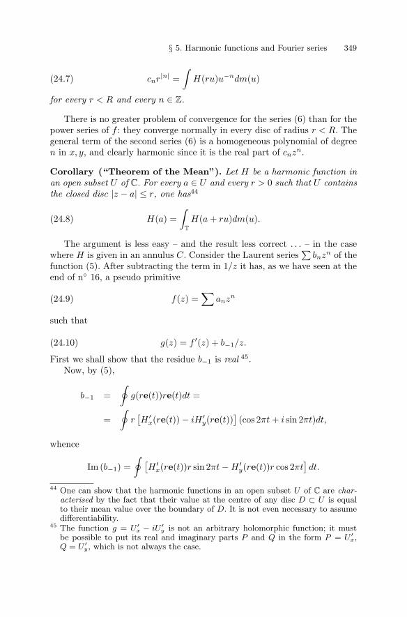
§ 5. Harmonic functions and Fourier series 349
cnr|n| =∫
H(ru)u−ndm(u)(24.7)
for every r < R and every n ∈ Z.
There is no greater problem of convergence for the series (6) than for thepower series of f : they converge normally in every disc of radius r < R. Thegeneral term of the second series (6) is a homogeneous polynomial of degreen in x, y, and clearly harmonic since it is the real part of cnzn.
Corollary (“Theorem of the Mean”). Let H be a harmonic function inan open subset U of C. For every a ∈ U and every r > 0 such that U containsthe closed disc |z − a| ≤ r, one has44
H(a) =∫
T
H(a + ru)dm(u).(24.8)
The argument is less easy – and the result less correct . . . – in the casewhere H is given in an annulus C. Consider the Laurent series
∑bnzn of the
function (5). After subtracting the term in 1/z it has, as we have seen at theend of n◦ 16, a pseudo primitive
f(z) =∑
anzn(24.9)
such that
g(z) = f ′(z) + b−1/z.(24.10)
First we shall show that the residue b−1 is real 45.Now, by (5),
b−1 =∮
g(re(t))re(t)dt =
=∮
r[H ′
x(re(t)) − iH ′y(re(t))
](cos 2πt + i sin 2πt)dt,
whence
Im (b−1) =∮ [
H ′x(re(t))r sin 2πt − H ′
y(re(t))r cos 2πt]dt.
44 One can show that the harmonic functions in an open subset U of C are char-acterised by the fact that their value at the centre of any disc D ⊂ U is equalto their mean value over the boundary of D. It is not even necessary to assumedifferentiability.
45 The function g = U ′x − iU ′
y is not an arbitrary holomorphic function; it mustbe possible to put its real and imaginary parts P and Q in the form P = U ′
x,Q = U ′
y, which is not always the case.
350 VII – Harmonic Analysis and Holomorphic Functions
Since re(t) has coordinates r cos(2πt) and r sin(2πt), the chain rule showsthat
d
dtH(re(t)) = −2π
[H ′
x(re(t))r sin 2πt − H ′y(re(t))r cos 2πt
];
consequently, Im (b−1) is, up to a factor −2π, the variation between 0 and 1of the function t → H(re(t)), zero by periodicity. The residue b−1 is thereforereal.
Now let us put f = P + iQ with P and Q real. It follows that
H ′x − iH ′
y = g(z) = P ′x − iP ′
y + b−1/(x + iy)
by (10), whence
H ′x = P ′
x + b−1x/(x2 + y2),H ′
y = P ′y + b−1y/(x2 + y2)
since b−1 is real. The function R = H − P thus satisfies the relations
R′x = b−1x/(x2 + y2),
R′y = b−1y/(x2 + y2).
Now the function
L(x, y) = log |z| = log r =12
log(x2 + y2
),
not to be confused with the pretend Log of the complex number z, has partialderivatives
L′x = x/(x2 + y2), L′
y = y/(x2 + y2).
The function R−b−1L thus has partial derivatives zero, so is constant, whenceit follows that
H(x, y) = P (x, y) + b−1 log r + const.(24.11)
Since f(z) = P (x, y) + iQ(x, y) =∑
anzn we find
H(z) = b log r + c +12
∑(anzn + anzn) =
= b log r + c +12
∑[an(x + iy)n + an(x − iy)n]
with real constants b and c, summing over all nonzero n ∈ Z. The expansion
H(ru) = b log r + c +12
∑n�=0
(anrn + a−nr−n
)un(24.12)
§ 5. Harmonic functions and Fourier series 351
is deduced from this, and yields the general form of the Fourier coefficientsof the function H(re(t)). One may put all this in the form
H(re(t)) = b. log r + c +∑n≥1
[bn(r) cos 2πnt + cn(r) sin 2πnt](24.13)
where the coefficients bn(r) and cn(r) are linear combinations with real co-efficients of rn and r−n.
Exercise. By using the equation ∆H = 0, show directly that the Fourierseries of u → H(ru) has the form (13). (Argue as in n◦ 14).
The fact that log r and the negative powers of r disappear when H isharmonic on a disc is due to the continuity of H on a neighbourhood ofthe origin: the Fourier coefficients of H(re(t)) must remain bounded when rtends to 0.
One of the consequences of these calculations is that, in an annulus, aharmonic function is not always the real part of a holomorphic function.This is the case only if b = 0 in the expansion (13); direct calculation of theFourier coefficients of H(ru) shows that
b log r + c =∫
H(ru)dm(u) =∮
H(re2πit)dt,(24.14)
the mean value of H over the circle |z| = r. One may explain the appearanceof the function log r by noting that it is the real part of the “function” Log z =log r + i arg z, which would be holomorphic for z �= 0 if one could forget theambiguity inherent in the definition of the argument; this ambiguity beingpure imaginary, the real part log r is, itself, a function in the strict sense –and it is harmonic. You can check this by calculating its Laplacian directly.
25 – Limits of harmonic functions
We have seen, in (24.8), that if a function H is harmonic on an open disc ofradius R, its value at the centre of the latter is equal to its mean value overevery concentric circle of radius r < R. We deduce that the maximum theorem(Theorem 11 of n◦ 15) and its corollary are valid for harmonic functions; theproofs are precisely the same. In particular, if a function is continuous on theclosure K of a bounded domain G and is harmonic in G, and is zero on theboundary F of G, then it is identically zero since ‖H‖G = ‖H‖F .
If a function H is harmonic on a disc |z| < R of radius R > 1 and if oneputs f(u) = H(u) on T, the series expansion
H(z) =∑
cnr|n|un with cnr|n| =∫
H(ru)u−ndm(u)
of Theorem 20, valid for r < R, holds in particular for r = 1 and shows thatcn = f(n). Hence
352 VII – Harmonic Analysis and Holomorphic Functions
H(z) = Hf (z) for |z| < 1.
In the case of an arbitrary radius R one can, for r < R, apply this result tothe function z → H(rz), harmonic in the disc of radius R/r > 1. Whence
H(rz) =∫
1 − |z|2|z − u|2 H(ru)dm(u) (|z| < 1),
or, on replacing z by z/r,
H(z) =∫
T
r2 − |z|2|z − ru|2 H(ru)dm(u) for |z| < r.(25.1)
This is the analogue for harmonic functions of Cauchy’s integral formula ofn◦ 1; the existence of such a formula is scarcely surprising, since, on a disc,a harmonic function is the real part of a holomorphic function.
Weierstrass’ theorem on uniformly convergent sequences of holomorphicfunctions applies also to harmonic functions, but needs several preliminaries.
First, the formula (24.6), i.e.
H(x, y) = c0 +∑n>0
[cn(x + iy)n + cn(x − iy)n] ,(25.2)
shows that a harmonic function is of class C∞; again not very surprising,since, locally, it is the real part of an analytic function. Further, if one differ-entiates the general term of the series (2) with respect to x or y one multipliesthe coefficients of order n by n or ±in; up to a factor of modulus 1 this isequivalent to replacing the two power series in x+ iy = z and x− iy = z thatappear in (24.6) by their derived series; the resulting series, and more gener-ally, those obtained by differentiating term-by-term ad libitum with respectto x and y, converge under exactly the same conditions as (2). Theorem 20of Chap. III, n◦ 17 would then show, if needed, that H is indefinitely dif-ferentiable and that its partial derivatives of arbitrary order are obtainedby differentiating the series (2) term-by-term with respect to x and y. (Thefact that we are dealing with functions of two variables is not important: thevariable with respect to which one is not differentiating plays the role of aconstant).
We deduce, after a small calculation, that the partial derivative
Dp1Dq
2H = H(p,q)
is given by
H(p,q)(x, y) ==∑
n(n − 1) . . . (n − p − q + 1) [iqcn(x + iy)n−p−q + (−i)qcn(x − iy)n−p−q]
where one sums over n ≥ p + q. In particular,
§ 5. Harmonic functions and Fourier series 353
H(p,q)(0, 0) = (p + q)! [iqcp+q + iqcp+q] = 2(p + q)!Re (iqcp+q) .
Since cnrn =∫
H(ru)u−ndm(u) for n ≥ 0 we have
H(p,q)(0, 0) = (p + q)!r−p−q
∫H(ru)
[iqu−p−q + (−i)qup+q
]dm(u)(25.3)
and consequently
∣∣∣H(p,q)(0, 0)∣∣∣ ≤ 2
(p + q)!rp+q
sup|u|=1
|H(ru)|.(25.4)
From this we have the analogue of Weierstrass’ convergence theorem:
Theorem 21. Let G an open set in C and (Hn) a sequence of harmonicfunctions in G which converges uniformly on every compact K ⊂ G to alimit function H. Then H is harmonic, and, for any p and q, the partialderivatives H
(p,q)n converge uniformly on every compact subset of G to the
partial derivative H(p,q) of H.
We know thanks to Borel-Lebesgue (Chap. V, n◦ 6) that uniform conver-gence on every compact subset is a property of local character: to verify itfor every compact K ⊂ G it is enough to show that, for every a ∈ G, it holdson a closed disc of centre a.
So choose an R > 0 such that the disc D : |z − a| ≤ R is contained in Gand put r = R/2. For every z such that |z−a| ≤ r the closed disc of centre zand of radius r is contained in D. By (4) we have, for every harmonic functionU in G,
U (p,q)(z) ≤ 2(p + q)!r−p−q sup|u|=1
|U(z + ru)|;
but for |z − a| ≤ r, all the points z + ru are in the large disc D, whencetrivially
sup|u|=1
|U(z + ru)| ≤ ‖U‖D ,
and consequently
U (p,q)(z) ≤ 2(p + q)!r−p−q. ‖U‖D for |z − a| ≤ r.
Now we apply the general result to the functions U = Hm − Hn. Since theHn converge uniformly on every compact subset of G, and in particular onD, we have ‖Hm − Hn‖D ≤ ε for m and n large. The preceding inequalitythen shows that, for m and n large, we have∣∣∣H(p,q)
m (z) − H(p,q)n (z)
∣∣∣ ≤ 2(p + q)!r−p−qε
at all the points of the disc |z − a| ≤ r.
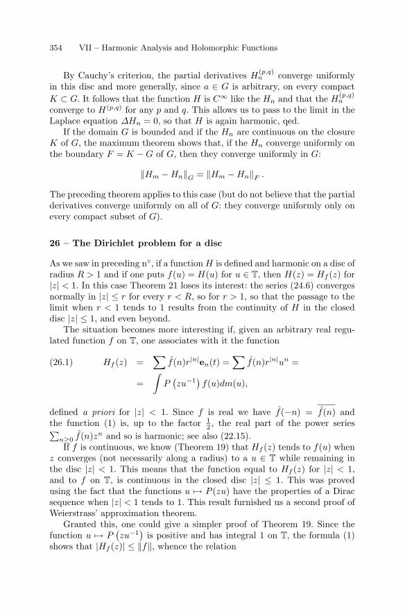
354 VII – Harmonic Analysis and Holomorphic Functions
By Cauchy’s criterion, the partial derivatives H(p,q)n converge uniformly
in this disc and more generally, since a ∈ G is arbitrary, on every compactK ⊂ G. It follows that the function H is C∞ like the Hn and that the H
(p,q)n
converge to H(p,q) for any p and q. This allows us to pass to the limit in theLaplace equation ∆Hn = 0, so that H is again harmonic, qed.
If the domain G is bounded and if the Hn are continuous on the closureK of G, the maximum theorem shows that, if the Hn converge uniformly onthe boundary F = K − G of G, then they converge uniformly in G:
‖Hm − Hn‖G = ‖Hm − Hn‖F .
The preceding theorem applies to this case (but do not believe that the partialderivatives converge uniformly on all of G: they converge uniformly only onevery compact subset of G).
26 – The Dirichlet problem for a disc
As we saw in preceding n◦, if a function H is defined and harmonic on a disc ofradius R > 1 and if one puts f(u) = H(u) for u ∈ T, then H(z) = Hf (z) for|z| < 1. In this case Theorem 21 loses its interest: the series (24.6) convergesnormally in |z| ≤ r for every r < R, so for r > 1, so that the passage to thelimit when r < 1 tends to 1 results from the continuity of H in the closeddisc |z| ≤ 1, and even beyond.
The situation becomes more interesting if, given an arbitrary real regu-lated function f on T, one associates with it the function
Hf (z) =∑
f(n)r|n|en(t) =∑
f(n)r|n|un =(26.1)
=∫
P(zu−1)f(u)dm(u),
defined a priori for |z| < 1. Since f is real we have f(−n) = f(n) andthe function (1) is, up to the factor 1
2 , the real part of the power series∑n≥0 f(n)zn and so is harmonic; see also (22.15).If f is continuous, we know (Theorem 19) that Hf (z) tends to f(u) when
z converges (not necessarily along a radius) to a u ∈ T while remaining inthe disc |z| < 1. This means that the function equal to Hf (z) for |z| < 1,and to f on T, is continuous in the closed disc |z| ≤ 1. This was provedusing the fact that the functions u → P (zu) have the properties of a Diracsequence when |z| < 1 tends to 1. This result furnished us a second proof ofWeierstrass’ approximation theorem.
Granted this, one could give a simpler proof of Theorem 19. Since thefunction u → P
(zu−1)
is positive and has integral 1 on T, the formula (1)shows that |Hf (z)| ≤ ‖f‖, whence the relation
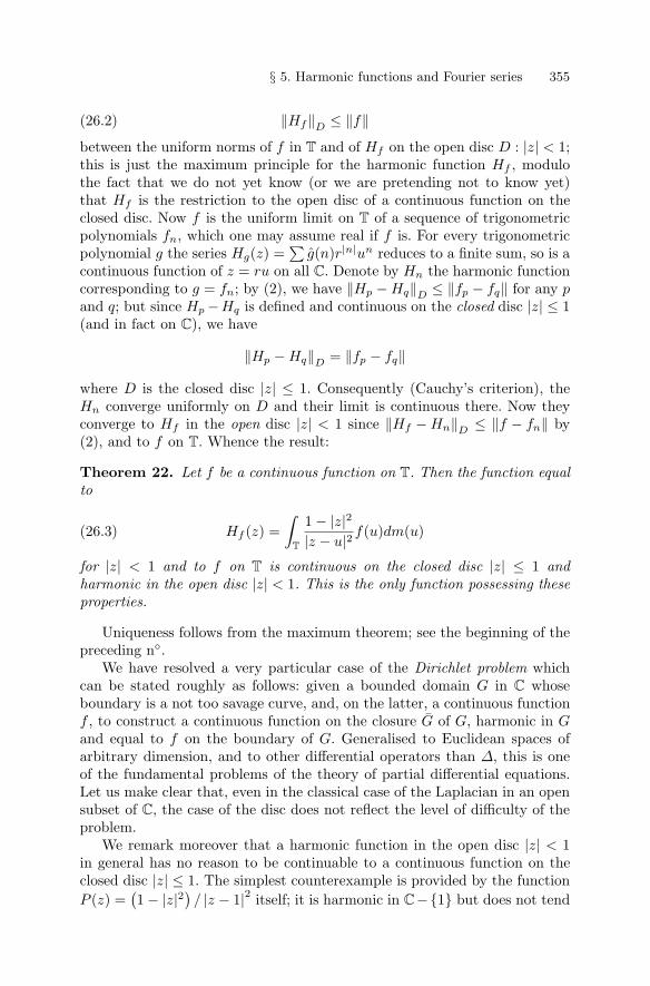
§ 5. Harmonic functions and Fourier series 355
‖Hf‖D ≤ ‖f‖(26.2)
between the uniform norms of f in T and of Hf on the open disc D : |z| < 1;this is just the maximum principle for the harmonic function Hf , modulothe fact that we do not yet know (or we are pretending not to know yet)that Hf is the restriction to the open disc of a continuous function on theclosed disc. Now f is the uniform limit on T of a sequence of trigonometricpolynomials fn, which one may assume real if f is. For every trigonometricpolynomial g the series Hg(z) =
∑g(n)r|n|un reduces to a finite sum, so is a
continuous function of z = ru on all C. Denote by Hn the harmonic functioncorresponding to g = fn; by (2), we have ‖Hp − Hq‖D ≤ ‖fp − fq‖ for any pand q; but since Hp −Hq is defined and continuous on the closed disc |z| ≤ 1(and in fact on C), we have
‖Hp − Hq‖D = ‖fp − fq‖
where D is the closed disc |z| ≤ 1. Consequently (Cauchy’s criterion), theHn converge uniformly on D and their limit is continuous there. Now theyconverge to Hf in the open disc |z| < 1 since ‖Hf − Hn‖D ≤ ‖f − fn‖ by(2), and to f on T. Whence the result:
Theorem 22. Let f be a continuous function on T. Then the function equalto
Hf (z) =∫
T
1 − |z|2|z − u|2 f(u)dm(u)(26.3)
for |z| < 1 and to f on T is continuous on the closed disc |z| ≤ 1 andharmonic in the open disc |z| < 1. This is the only function possessing theseproperties.
Uniqueness follows from the maximum theorem; see the beginning of thepreceding n◦.
We have resolved a very particular case of the Dirichlet problem whichcan be stated roughly as follows: given a bounded domain G in C whoseboundary is a not too savage curve, and, on the latter, a continuous functionf , to construct a continuous function on the closure G of G, harmonic in Gand equal to f on the boundary of G. Generalised to Euclidean spaces ofarbitrary dimension, and to other differential operators than ∆, this is oneof the fundamental problems of the theory of partial differential equations.Let us make clear that, even in the classical case of the Laplacian in an opensubset of C, the case of the disc does not reflect the level of difficulty of theproblem.
We remark moreover that a harmonic function in the open disc |z| < 1in general has no reason to be continuable to a continuous function on theclosed disc |z| ≤ 1. The simplest counterexample is provided by the functionP (z) =
(1 − |z|2) / |z − 1|2 itself; it is harmonic in C−{1} but does not tend
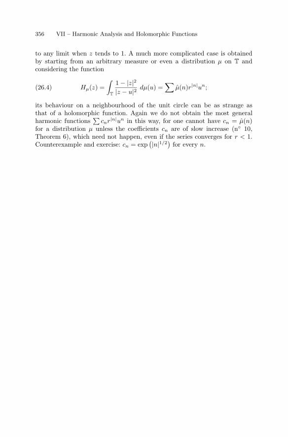
356 VII – Harmonic Analysis and Holomorphic Functions
to any limit when z tends to 1. A much more complicated case is obtainedby starting from an arbitrary measure or even a distribution µ on T andconsidering the function
Hµ(z) =∫
T
1 − |z|2|z − u|2 dµ(u) =
∑µ(n)r|n|un;(26.4)
its behaviour on a neighbourhood of the unit circle can be as strange asthat of a holomorphic function. Again we do not obtain the most generalharmonic functions
∑cnr|n|un in this way, for one cannot have cn = µ(n)
for a distribution µ unless the coefficients cn are of slow increase (n◦ 10,Theorem 6), which need not happen, even if the series converges for r < 1.Counterexample and exercise: cn = exp
(|n|1/2)
for every n.
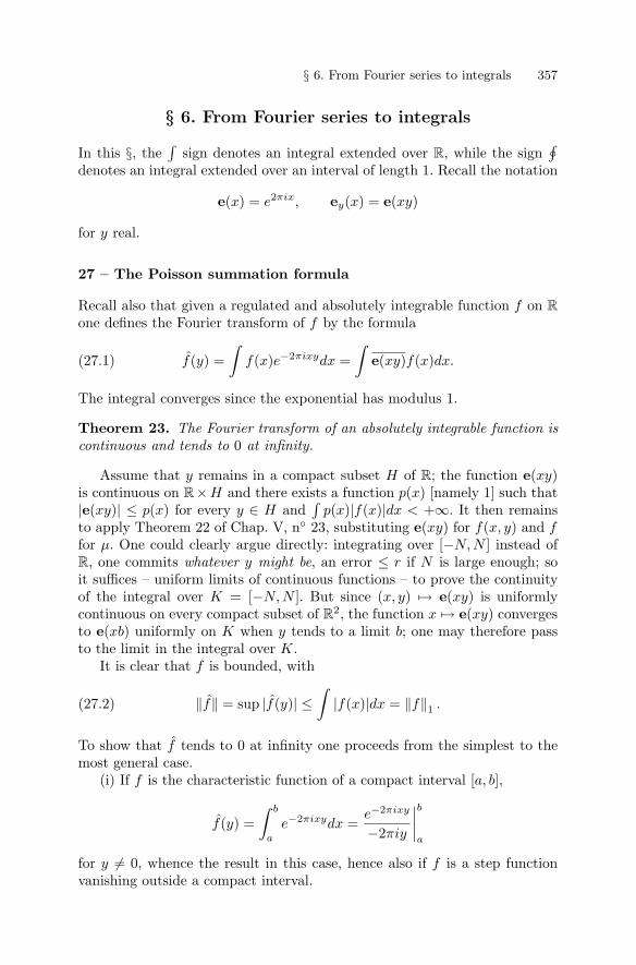
§ 6. From Fourier series to integrals 357
§ 6. From Fourier series to integrals
In this §, the∫
sign denotes an integral extended over R, while the sign∮
denotes an integral extended over an interval of length 1. Recall the notation
e(x) = e2πix, ey(x) = e(xy)
for y real.
27 – The Poisson summation formula
Recall also that given a regulated and absolutely integrable function f on Rone defines the Fourier transform of f by the formula
f(y) =∫
f(x)e−2πixydx =∫
e(xy)f(x)dx.(27.1)
The integral converges since the exponential has modulus 1.
Theorem 23. The Fourier transform of an absolutely integrable function iscontinuous and tends to 0 at infinity.
Assume that y remains in a compact subset H of R; the function e(xy)is continuous on R×H and there exists a function p(x) [namely 1] such that|e(xy)| ≤ p(x) for every y ∈ H and
∫p(x)|f(x)|dx < +∞. It then remains
to apply Theorem 22 of Chap. V, n◦ 23, substituting e(xy) for f(x, y) and ffor µ. One could clearly argue directly: integrating over [−N, N ] instead ofR, one commits whatever y might be, an error ≤ r if N is large enough; soit suffices – uniform limits of continuous functions – to prove the continuityof the integral over K = [−N, N ]. But since (x, y) → e(xy) is uniformlycontinuous on every compact subset of R2, the function x → e(xy) convergesto e(xb) uniformly on K when y tends to a limit b; one may therefore passto the limit in the integral over K.
It is clear that f is bounded, with
‖f‖ = sup |f(y)| ≤∫
|f(x)|dx = ‖f‖1 .(27.2)
To show that f tends to 0 at infinity one proceeds from the simplest to themost general case.
(i) If f is the characteristic function of a compact interval [a, b],
f(y) =∫ b
a
e−2πixydx =e−2πixy
−2πiy
∣∣∣∣ba
for y �= 0, whence the result in this case, hence also if f is a step functionvanishing outside a compact interval.
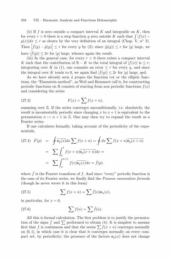
358 VII – Harmonic Analysis and Functions Holomorphic
(ii) If f is zero outside a compact interval K and integrable on K, thenfor every r > 0 there is a step function g zero outside K such that
∫ |f(x)−g(x)|dx ≤ r as shown by the very definition of an integral (Chap. V, n◦ 2).Then∣∣∣f(y) − g(y)
∣∣∣ ≤ r for every y by (2); since |g(y)| ≤ r for |y| large, we
have |f(y)| ≤ 2r for |y| large, whence again the result.(iii) In the general case, for every r > 0 there exists a compact interval
K such that the contribution of R − K to the total integral of |f(x)| is ≤ r;integrating over K in (1), one commits an error ≤ r for every y, and sincethe integral over K tends to 0, we again find |f(y)| ≤ 2r for |y| large, qed.
As we have already seen a propos the function cot or the elliptic func-tions, the “Eisenstein method”, as Weil and Remmert call it, for constructingperiodic functions on R consists of starting from non periodic functions f(x)and considering the series
F (x) =∑
f(x + n),(27.3)
summing over Z. If the series converges unconditionally, i.e. absolutely, theresult is incontestably periodic since changing x to x + 1 is equivalent to thepermutation n → n + 1 in Z. One may then try to expand the result as aFourier series.
If one calculates formally, taking account of the periodicity of the expo-nentials,
F (p) =∮
ep(x)dx∑
f(x + n) =∮
dx∑
f(x + n)ep(x + n)(27.4)
=∑∫ 1
0
f(x + n)ep(x + n)dx =
=∑∫ n+1
n
f(x)ep(x)dx = f(p).
where f is the Fourier transform of f . And since “every” periodic function isthe sum of its Fourier series, we finally find the Poisson summation formula(though he never wrote it in this form)∑
f(x + n) =∑
f(n)en(x),(27.5)
in particular, for x = 0, ∑f(n) =
∑f(n).(27.6)
All this is formal calculation. The first problem is to justify the permuta-tion of the signs
∫and∑
performed to obtain (4). It is simplest to assumefirst that f is continuous and that the series
∑f(x + n) converges normally
on [0, 1], in which case it is clear that it converges normally on every com-pact set, by periodicity; the presence of the factors ep(x) does not change
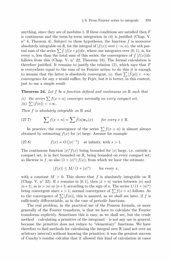
§ 6. From Fourier series to integrals 359
anything, since they are of modulus 1. If these conditions are satisfied then Fis continuous and the term-by-term integration in (4) is justified (Chap. V,n◦ 4, Theorem 4). Subject to these hypotheses, the function f is moreoverabsolutely integrable on R, for the integral of |f(x)| over (−n, n), the nth par-tial sum of the series
∑∫ |f(x+p)|dx, where one integrates over (0, 1), is, forevery n, less than the total sum of this series; the convergence of
∫ |f(x)|dxfollows from this (Chap. V, n◦ 22, Theorem 18). The formal calculation istherefore justified. It remains to justify the relation (5), which says that Fis everywhere equal to the sum of its Fourier series; to do this it is enoughto assume that the latter is absolutely convergent, i.e. that
∑ |f(p)| < +∞;convergence for any x would suffice, by Fejer, but it is better, in this context,just to use a simple result:
Theorem 24. Let f be a function defined and continuous on R such that
(i) the series∑
f(x + n) converges normally on every compact set,(ii)∑ |f(n)| < +∞.
Then f is absolutely integrable on R and∑f(x + n) =
∑f(n)en(x) for every x ∈ R.(27.7)
In practice, the convergence of the series∑
f(x + n) is almost alwaysobtained by estimating f(x) for |x| large. Assume for example
f(x) = O(|x|−s)
at infinity, with s > 1.(27.8)
The continuous function |x|sf(x) being bounded for |x| large, i.e. outside acompact set, is in fact bounded on R, being bounded on every compact set;so likewise is f , so also (1 + |x|s) f(x), from which we have the estimate
|f(x)| ≤ M/ (1 + |x|s) for every x,
with a constant M > 0. This shows that f is absolutely integrable on R(Chap. V, n◦ 22). If x remains in [0, 1], then |x + n| varies between |n| and|n+1|, so is > |n| or |n+1| according to the sign of n. The series 1/ (1 + |n|s)being convergent since s > 1, normal convergence of
∑f(x + n) follows. As
to the convergence of∑ |f(n)|, this is assured, as we shall see later, if f is
sufficiently differentiable, as in the case of periodic functions.The real problem, in the practical use of the Poisson formula, or more
generally of the Fourier transform, is that we have to calculate the Fouriertransforms explicitly. Sometimes this is easy, as we shall see, but the crudemethod – calculating a primitive of the integrand – is not any use in general,because the primitive does not reduce to “elementary” functions. We havetherefore to find methods for calculating the integral over R (and not over anarbitrary interval) without knowing the primitive; it was the greatest successof Cauchy’s residue calculus that it allowed this kind of calculation in cases

360 VII – Harmonic Analysis and Functions Holomorphic
unknown up till then. Nothing better has been found since then; we havemany formulae for Fourier transforms in terms of special functions, Euler’sΓ function for example, but they are almost always obtained by Cauchy’smethod.
Example 1. Choose the function
f(t) = 1/(z + t)s
where z is a non real complex parameter and s an integer ≥ 2, with for exam-ple Im(z) > 0. The preceding considerations show that the series
∑f(t + n)
is normally convergent on every compact set, but it remains to calculate theFourier transform
f(n) =∫
exp(−2πint) (z + t)−sdt
for n real, not necessarily an integer. To seek a primitive, for example byintegrating by parts, would lead, more complication, to integrals of the typeexxndx of Chap. V, n◦ 15, Example 2; they can be calculated immediatelyby hand for n an integer > 0 but, for n < 0, and especially for n = −2,they resist every attempt at explicit calculation (and not only because weare working here at too elementary a level); Euler’s gamma function wouldnot have survived if one had been able to calculate a primitive of e−xxs.But, with his residue method, Cauchy succeeded in calculating in a generalway the Fourier transform of a rational function p/q having no real pole anddecreasing sufficiently fast at infinity, i.e. such that d(q) > d(p) + 1. We mayprove for example that, for s integer ≥ 2 (convergence!), we have
∫exp(−2πiut) (z + t)−s
dt =
⎧⎨⎩
(−2πi)sus−1 exp(2πiuz)/(s − 1)! if u > 0,
0 if u ≤ 0(27.9)on condition that Im(z) > 0. The summation formula
∑f(n) =
∑f(n) can
be written, in this case, as
∑Z
1(z + n)s
=(−2πi)s
(s − 1)!
∑n>0
ns−1e2πinz for Im(z) > 0.(27.10)
For s = 2, this is ∑Z
1/(z − n)2 = −4π2∑
N
ne2πinz;(27.11)
now we know (see (8.14) for example) that, for z not an integer, the left handside is equal to π2/ sin2 πz; for Im(z) > 0 we have
∣∣eiz∣∣ < 1 and so
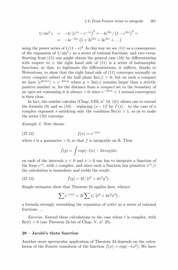
§ 6. From Fourier series to integrals 361
1/ sin2 z = −4/(eiz − e−iz
)2= −4e2iz/
(1 − e2iz
)2=
= −4e−2iz(1 + 2e2iz + 3e4iz + . . .
)using the power series of 1/(1−x)2. In this way we see (11) as a consequenceof the expansion of 1/ sin2 z as a series of rational fractions, and vice-versa.Starting from (11) one might obtain the general case (10) by differentiatingwith respect to z: the right hand side of (11) is a series of holomorphicfunctions, so that, to legitimate the differentiations, it suffices, thanks toWeierstrass, to show that the right hand side of (11) converges normally onevery compact subset of the half plane Im(z) > 0; but on such a compactwe have
∣∣e2πinz∣∣ = e−2πny where y = Im(z) remains larger than a strictly
positive number m, for the distance from a compact set to the boundary ofan open set containing it is always > 0; since e−2πm < 1 normal convergenceis then clear.
In fact, the residue calculus (Chap. VIII, n◦ 10, (ii)) allows one to extendthe formula (9) and so (10) – replacing (s − 1)! by Γ (s) – to the case of acomplex exponent s satisfying only the condition Re(s) > 1, so as to makethe series (10) converge.
Example 2. Now choose
f(x) = e−t|x|(27.12)
where t is a parameter > 0, so that f is integrable on R. Then
f(y) =∫
exp(−t|x| − 2πixy)dx;
on each of the intervals x < 0 and x > 0 one has to integrate a function ofthe form ecx, with c complex, and since such a function has primitive ecx/cthe calculation is immediate and yields the result:
f(y) = 2t/(t2 + 4π2y2
).(27.13)
Simple estimates show that Theorem 24 applies here, whence∑e−|n|t = 2t
∑1/(t2 + 4π2n2
),
a formula strongly resembling the expansion of coth t as a series of rationalfractions . . .
Exercise. Extend these calculations to the case where t is complex, withRe(t) > 0 (use Theorem 24 bis of Chap. V, n◦ 25).
28 – Jacobi’s theta function
Another more spectacular application of Theorem 24 depends on the calcu-lation of the Fourier transform of the function f(x) = exp(−πx2). We have
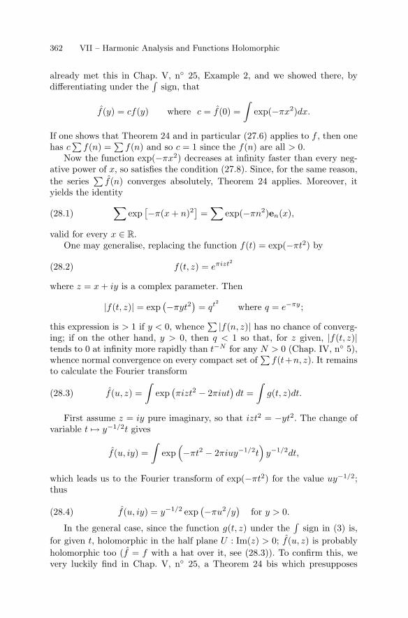
362 VII – Harmonic Analysis and Functions Holomorphic
already met this in Chap. V, n◦ 25, Example 2, and we showed there, bydifferentiating under the
∫sign, that
f(y) = cf(y) where c = f(0) =∫
exp(−πx2)dx.
If one shows that Theorem 24 and in particular (27.6) applies to f , then onehas c∑
f(n) =∑
f(n) and so c = 1 since the f(n) are all > 0.Now the function exp(−πx2) decreases at infinity faster than every neg-
ative power of x, so satisfies the condition (27.8). Since, for the same reason,the series
∑f(n) converges absolutely, Theorem 24 applies. Moreover, it
yields the identity∑exp[−π(x + n)2
]=∑
exp(−πn2)en(x),(28.1)
valid for every x ∈ R.One may generalise, replacing the function f(t) = exp(−πt2) by
f(t, z) = eπizt2(28.2)
where z = x + iy is a complex parameter. Then
|f(t, z)| = exp(−πyt2
)= qt2 where q = e−πy;
this expression is > 1 if y < 0, whence∑ |f(n, z)| has no chance of converg-
ing; if on the other hand, y > 0, then q < 1 so that, for z given, |f(t, z)|tends to 0 at infinity more rapidly than t−N for any N > 0 (Chap. IV, n◦ 5),whence normal convergence on every compact set of
∑f(t+n, z). It remains
to calculate the Fourier transform
f(u, z) =∫
exp(πizt2 − 2πiut
)dt =∫
g(t, z)dt.(28.3)
First assume z = iy pure imaginary, so that izt2 = −yt2. The change ofvariable t → y−1/2t gives
f(u, iy) =∫
exp(−πt2 − 2πiuy−1/2t
)y−1/2dt,
which leads us to the Fourier transform of exp(−πt2) for the value uy−1/2;thus
f(u, iy) = y−1/2 exp(−πu2/y
)for y > 0.(28.4)
In the general case, since the function g(t, z) under the∫
sign in (3) is,for given t, holomorphic in the half plane U : Im(z) > 0; f(u, z) is probablyholomorphic too (f = f with a hat over it, see (28.3)). To confirm this, wevery luckily find in Chap. V, n◦ 25, a Theorem 24 bis which presupposes
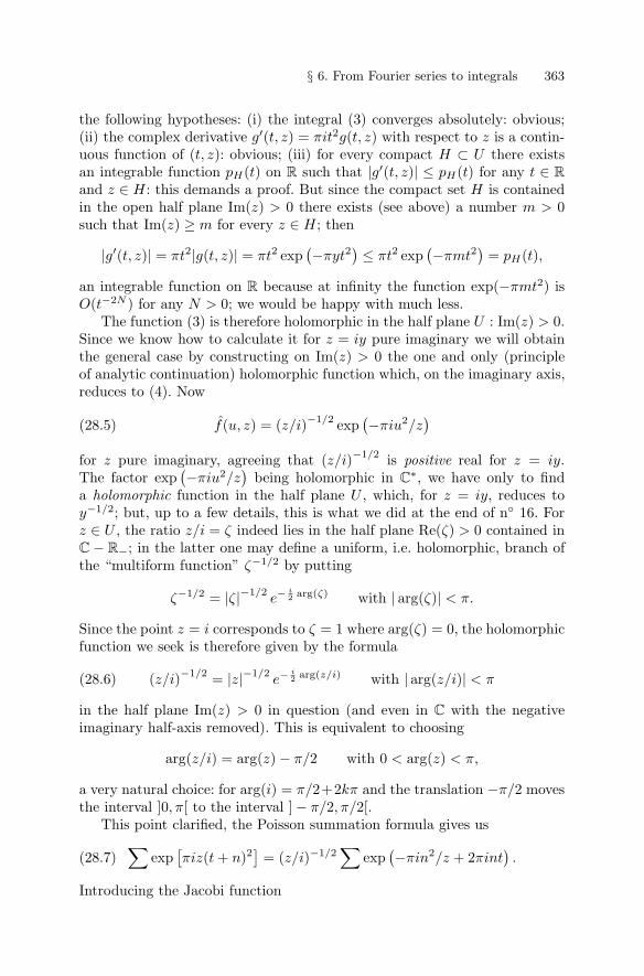
§ 6. From Fourier series to integrals 363
the following hypotheses: (i) the integral (3) converges absolutely: obvious;(ii) the complex derivative g′(t, z) = πit2g(t, z) with respect to z is a contin-uous function of (t, z): obvious; (iii) for every compact H ⊂ U there existsan integrable function pH(t) on R such that |g′(t, z)| ≤ pH(t) for any t ∈ Rand z ∈ H: this demands a proof. But since the compact set H is containedin the open half plane Im(z) > 0 there exists (see above) a number m > 0such that Im(z) ≥ m for every z ∈ H; then
|g′(t, z)| = πt2|g(t, z)| = πt2 exp(−πyt2
) ≤ πt2 exp(−πmt2
)= pH(t),
an integrable function on R because at infinity the function exp(−πmt2) isO(t−2N ) for any N > 0; we would be happy with much less.
The function (3) is therefore holomorphic in the half plane U : Im(z) > 0.Since we know how to calculate it for z = iy pure imaginary we will obtainthe general case by constructing on Im(z) > 0 the one and only (principleof analytic continuation) holomorphic function which, on the imaginary axis,reduces to (4). Now
f(u, z) = (z/i)−1/2 exp(−πiu2/z
)(28.5)
for z pure imaginary, agreeing that (z/i)−1/2 is positive real for z = iy.The factor exp
(−πiu2/z)
being holomorphic in C∗, we have only to finda holomorphic function in the half plane U , which, for z = iy, reduces toy−1/2; but, up to a few details, this is what we did at the end of n◦ 16. Forz ∈ U , the ratio z/i = ζ indeed lies in the half plane Re(ζ) > 0 contained inC − R−; in the latter one may define a uniform, i.e. holomorphic, branch ofthe “multiform function” ζ−1/2 by putting
ζ−1/2 = |ζ|−1/2e−
i2 arg(ζ) with | arg(ζ)| < π.
Since the point z = i corresponds to ζ = 1 where arg(ζ) = 0, the holomorphicfunction we seek is therefore given by the formula
(z/i)−1/2 = |z|−1/2e−
i2 arg(z/i) with | arg(z/i)| < π(28.6)
in the half plane Im(z) > 0 in question (and even in C with the negativeimaginary half-axis removed). This is equivalent to choosing
arg(z/i) = arg(z) − π/2 with 0 < arg(z) < π,
a very natural choice: for arg(i) = π/2+2kπ and the translation −π/2 movesthe interval ]0, π[ to the interval ] − π/2, π/2[.
This point clarified, the Poisson summation formula gives us∑exp[πiz(t + n)2
]= (z/i)−1/2
∑exp(−πin2/z + 2πint
).(28.7)
Introducing the Jacobi function
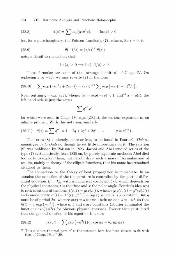
364 VII – Harmonic Analysis and Functions Holomorphic
θ(z) =∑
exp(πin2z), Im(z) > 0(28.8)
(or, for z pure imaginary, the Poisson function), (7) reduces, for t = 0, to
θ(−1/z) = (z/i)1/2θ(z);(28.9)
note, a detail to remember, that
Im(z) > 0 =⇒ Im(−1/z) > 0.
These formulae are some of the “strange identities” of Chap. IV. Onreplacing z by −1/z we may rewrite (7) in the form∑
exp(πin2z + 2πint
)= (z/i)1/2
∑exp[−πi(t + n)2/z
].(28.10)
Now, putting q = exp(πiz), whence |q| = exp(−πy) < 1, and46 x = e(t), theleft hand side is just the series ∑
qn2xn
for which we wrote, in Chap. IV, eqn. (20.14), the curious expansion as aninfinite product. With this notation, similarly
θ(z) =∑
qn2= 1 + 2q + 2q4 + 2q9 + . . .
(q = eπiz
).(28.11)
The series (8) is already, more or less, to be found in Fourier’s Theorieanalytique de la chaleur, though he set little importance on it. The relation(9) was published by Poisson in 1823. Jacobi and Abel studied series of thetype (7) systematically, from 1825 on, by purely algebraic methods; Abel diedtoo early to exploit them, but Jacobi drew such a mass of formulae and ofresults, mainly in theory of the elliptic functions, that his name has remainedattached to them.
The connection to the theory of heat propagation is immediate. In anannulus the evolution of the temperature is controlled by the partial differ-ential equation f ′
t = f ′′xx with a numerical coefficient > 0 which depends on
the physical constants; t is the time and x the polar angle. Fourier’s idea wasto seek solutions of the form f(x, t) = g(x)h(t), whence g(x)h′(t) = g′′(x)h(t)and consequently h′(t) = λh(t), g′′(x) = λg(x) where λ is a constant. But gmust be of period 2π, whence g(x) = a cos nx+b sin nx and λ = −n2, so thath(t) = c. exp
(−n2t), where a, b and c are constants (Fourier eliminated the
functions exp(+n2t) for obvious physical reasons). Fourier then postulatedthat the general solution of his equation is a sum
f(x, t) =∑
exp(−n2t)(an cos nx + bn sin nx)(28.12)
46 This x is not the real part of z; the notation here has been chosen to fit withthat of Chap. IV, n◦ 20.
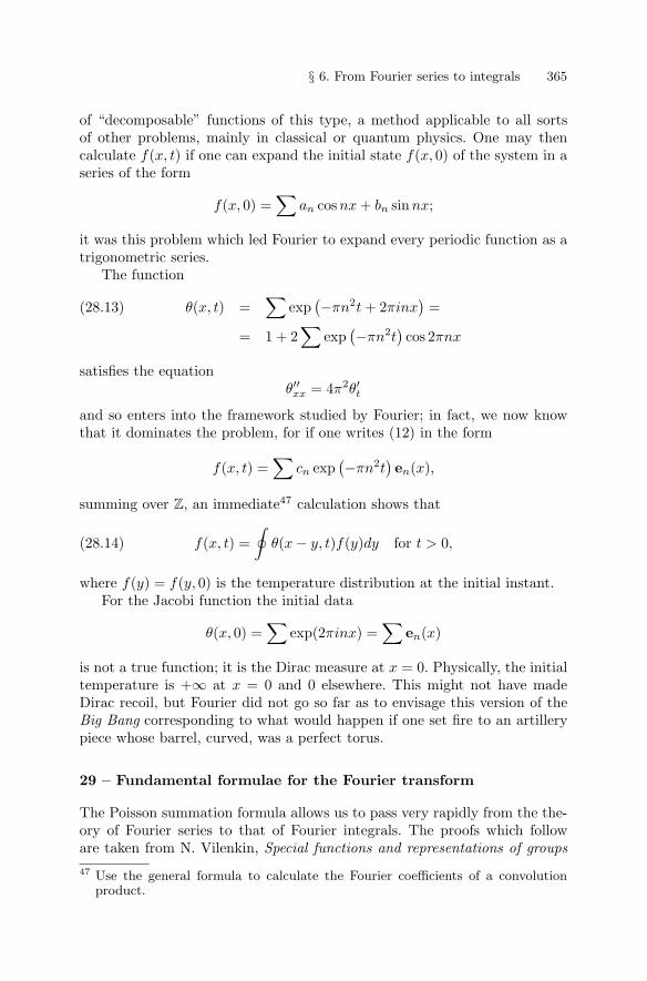
§ 6. From Fourier series to integrals 365
of “decomposable” functions of this type, a method applicable to all sortsof other problems, mainly in classical or quantum physics. One may thencalculate f(x, t) if one can expand the initial state f(x, 0) of the system in aseries of the form
f(x, 0) =∑
an cos nx + bn sin nx;
it was this problem which led Fourier to expand every periodic function as atrigonometric series.
The function
θ(x, t) =∑
exp(−πn2t + 2πinx
)=(28.13)
= 1 + 2∑
exp(−πn2t
)cos 2πnx
satisfies the equationθ′′xx = 4π2θ′t
and so enters into the framework studied by Fourier; in fact, we now knowthat it dominates the problem, for if one writes (12) in the form
f(x, t) =∑
cn exp(−πn2t
)en(x),
summing over Z, an immediate47 calculation shows that
f(x, t) =∮
θ(x − y, t)f(y)dy for t > 0,(28.14)
where f(y) = f(y, 0) is the temperature distribution at the initial instant.For the Jacobi function the initial data
θ(x, 0) =∑
exp(2πinx) =∑
en(x)
is not a true function; it is the Dirac measure at x = 0. Physically, the initialtemperature is +∞ at x = 0 and 0 elsewhere. This might not have madeDirac recoil, but Fourier did not go so far as to envisage this version of theBig Bang corresponding to what would happen if one set fire to an artillerypiece whose barrel, curved, was a perfect torus.
29 – Fundamental formulae for the Fourier transform
The Poisson summation formula allows us to pass very rapidly from the the-ory of Fourier series to that of Fourier integrals. The proofs which followare taken from N. Vilenkin, Special functions and representations of groups47 Use the general formula to calculate the Fourier coefficients of a convolution
product.
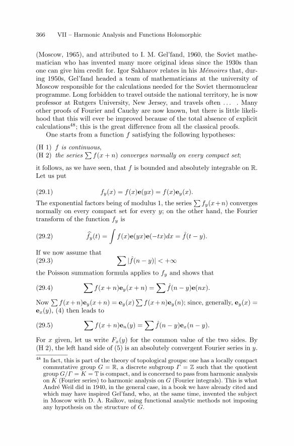
366 VII – Harmonic Analysis and Functions Holomorphic
(Moscow, 1965), and attributed to I. M. Gel’fand, 1960, the Soviet mathe-matician who has invented many more original ideas since the 1930s thanone can give him credit for. Igor Sakharov relates in his Memoires that, dur-ing 1950s, Gel’fand headed a team of mathematicians at the university ofMoscow responsible for the calculations needed for the Soviet thermonuclearprogramme. Long forbidden to travel outside the national territory, he is nowprofessor at Rutgers University, New Jersey, and travels often . . . . Manyother proofs of Fourier and Cauchy are now known, but there is little likeli-hood that this will ever be improved because of the total absence of explicitcalculations48; this is the great difference from all the classical proofs.
One starts from a function f satisfying the following hypotheses:
(H 1) f is continuous,(H 2) the series
∑f(x + n) converges normally on every compact set;
it follows, as we have seen, that f is bounded and absolutely integrable on R.Let us put
fy(x) = f(x)e(yx) = f(x)ey(x).(29.1)
The exponential factors being of modulus 1, the series∑
fy(x+n) convergesnormally on every compact set for every y; on the other hand, the Fouriertransform of the function fy is
fy(t) =∫
f(x)e(yx)e(−tx)dx = f(t − y).(29.2)
If we now assume that ∑|f(n − y)| < +∞(29.3)
the Poisson summation formula applies to fy and shows that∑f(x + n)ey(x + n) =
∑f(n − y)e(nx).(29.4)
Now∑
f(x+n)ey(x+n) = ey(x)∑
f(x+n)ey(n); since, generally, ey(x) =ex(y), (4) then leads to∑
f(x + n)en(y) =∑
f(n − y)ex(n − y).(29.5)
For x given, let us write Fx(y) for the common value of the two sides. By(H 2), the left hand side of (5) is an absolutely convergent Fourier series in y.48 In fact, this is part of the theory of topological groups: one has a locally compact
commutative group G = R, a discrete subgroup Γ = Z such that the quotientgroup G/Γ = K = T is compact, and is concerned to pass from harmonic analysison K (Fourier series) to harmonic analysis on G (Fourier integrals). This is whatAndre Weil did in 1940, in the general case, in a book we have already cited andwhich may have inspired Gel’fand, who, at the same time, invented the subjectin Moscow with D. A. Raıkov, using functional analytic methods not imposingany hypothesis on the structure of G.
§ 6. From Fourier series to integrals 367
The coefficients f(x+n) are therefore found by integration (Chap. V, n◦ 5).Whence, for n = 0,
f(x) =∫ 1
0
Fx(y)dy =∫ 1
0
dy∑
f(n − y)ex(n − y).
Let us now strengthen the hypothesis (3) and suppose
(H 3) the series∑
f(y + n) converges normally on every compact set;
then so does the series to be integrated, whence
f(x) =∑∮
f(n − y)ex(n − y)dy =
=∑∮
f(n + y)ex(n + y)dy,
which is simply the Fourier inversion formula
f(x) =∫
f(y)e(xy)dy =∫
f(y)e2πixydy(29.6)
where one integrates over R. We may write
f(x) = f(−x).(29.6’)
Let us now apply the Parseval-Bessel equality to (5), considered as aFourier series in y. We find the relation
∑|f(x + n)|2 =
∮dy∣∣∣∑ f(n − y)e2πix(n−y)
∣∣∣2(29.7)
=∮
dy∣∣∣∑ f(n − y)e2πinx
∣∣∣2since e2πixy, of modulus 1, is a factor of the series on the right hand side; theseries on the left hand side is convergent by Parseval-Bessel, but since f isbounded,
|f(x + n)|2 ≤ ‖f‖.|f(x + n)|;(29.8)
so the series (7) converges normally on every compact set, by (H 2), and itssum is continuous.
Now let us integrate with respect to x over (0, 1); we find∫ |f(x)|2 dx,
a convergent integral by (8) and the fact that∫ |f(x)|dx converges. On the
right hand side the function∑
f(n − y)en(x) is continuous in (y, x), for if aconvergent series
∑v(n) dominates the series
∑ |f(n−y)| on I = [0, 1], thenit dominates the series in question on I × R. We may therefore interchange
368 VII – Harmonic Analysis and Functions Holomorphic
the order of integration (Chap. V, n◦ 9, Theorem 10), to obtain the doubleintegral ∫ 1
0
dy
∫ 1
0
dx∣∣∣∑ f(n − y)en(x)
∣∣∣2 .
But the function to be integrated is, for y given, the square of an absolutelyconvergent Fourier series in x. Its integral may therefore be calculated usingParseval-Bessel (Chap. V, n◦ 5 suffices), i.e. is equal to
∑ |f(n − y)|2. Onintegrating with respect to y and comparing with the preceding result wefinally obtain the Plancherel formula∫
|f(x)|2dx =∫
|f(y)|2dy;(29.9)
this is the analogue of Parseval-Bessel for Fourier integrals. In conclusion:
Theorem 25. Let f be a continuous and absolutely integrable function on Rsuch that the series
∑f(x + n) and
∑f(y + n) converge normally on every
compact set. Then
f(x) =∫
f(y)e(xy)dy,
∫|f(x)|2dx =
∫|f(y)|2dy,
the three integrals over R being absolutely convergent.
More generally, if two functions f and g satisfy the hypotheses of thetheorem, then ∫
f(x)g(x)dx =∫
f(y)g(y)dy;(29.10)
one passes from the case f = g to the general case as we did for Fourierseries, i.e. by applying the Plancherel formula to the functions f + g, f − g,f + ig and f − ig.
Example. In view of Example 2 of n◦ 27 we have∫2te2πixy
t2 + 4π2y2dy = e−t|x| for every t > 0.
This formula essentially says no more than∫eixydy
x2 + 1= πe−|x|.
Cauchy’s residue calculus would give this formula directly. To try to establishit “without knowing anything” is hopeless, except of course for x = 0, theonly case where the primitive can be calculated.
Exercise (another proof of the inversion formula). Let f be a continuousfunction on R satisfying
§ 6. From Fourier series to integrals 369
f(x) = O (1/|x|a) , f(y) = O(1/|y|b)
at infinity, with constants a, b > 1, so that f and f are absolutely integrable.(i) Show that the Poisson summation formula applies to f [use Theorem 2of n◦ 6]. (ii) Show that, for every T > 0,
∑f(x + nT ) =
1T
∑f(n/T )e2πinx/T .
(iii) Show that, when T → +∞, the left hand side tends to f(x) and theother to
∫f(y)e(xy)dy.
30 – Extensions of the inversion formula
One may also write (29.10) in the often convenient form∫f(x)g(x)dx =
∫f(y)g(y)dy;(30.1)
it suffices, in (29.10), to replace g(x) by g(x) and to note that then g(y) isreplaced by g(y). The relation (1) is in fact directly obvious if one calculatesformally:∫
f(x)g(x)dx =(30.2)
=∫
f(x)dx
∫g(y)e(xy)dy =
∫ ∫f(x)g(y)e(xy)dxdy =
=∫
g(y)dy
∫f(x)e(xy)dx =
∫f(y)g(y)dy.
But one has to justify the interchange of the integrations. In the Lebesguetheory it is enough to assume that h(x, y) = f(x)g(y)e(xy) is integrable onR2, i.e. that f and g are integrable, since e(xy) is continuous and bounded;one then applies Fubini’s theorem (the real one . . .) to the function obtained.
In the Riemann theory, there is a more restricted, but nevertheless usefulresult:
Lemma. Let f and g be two absolutely integrable regulated functions; then∫f(x)g(x)dx =
∫f(y)g(y)dy.
First assume f and g are zero outside compact intervals K and H,and consider on K and H the measures dµ(x) = f(x)dx, dν(y) = g(y)dy(Chap. V, n◦ 30, Example 1). Since the function e(xy) is continuous onK × H we have∫
dµ(x)∫
e(xy)dν(y) =∫
dν(y)∫
e(xy)dµ(x)
370 VII – Harmonic Analysis and Functions Holomorphic
(Chap. V, n◦ 30, Theorem 30). By definition of µ and ν, this relation justifiesthe formal calculation (2). The lemma is therefore true under the hypothesesjust formulated.
In the general case, let us write fn and gn for the functions equal to fand g on [−n, n] and zero elsewhere, whence∫
fn(x)gn(x)dx =∫
fn(y)gn(y)dy.(30.3)
It all reduces to showing that one may pass to the limit under the integra-tion sign. Let us do this for the left hand side. It is enough to show that‖fngn − fg‖1 tends to 0, since, generally,
∣∣∫ f∣∣ ≤ ∫ |f |. Now omitting the
variable x,
|fngn − fg| ≤ |fn − f | . |gn| + |f |. |gn − g|≤ |fn − f | . ‖gn‖ + |f |. ‖gn − g‖≤ |fn − f | . ‖gn‖1 + |f |. ‖gn − g‖1
since
‖g‖ = sup |g(x)| = sup∣∣∣∣∫
e(xy)g(y)dy
∣∣∣∣ ≤ ‖g‖1
for every absolutely integrable function on R. Whence, integrating over R,
‖fngn − fg‖1 ≤ ‖fn − f‖1 . ‖gn‖1 + ‖f‖1. ‖gn − g‖1(30.4)
But‖fn − f‖1 =
∫|x|>n
|f(x)|dx
tends to 0 since f is absolutely integrable, likewise ‖gn − g‖1; the factor ‖f‖1
is independent of n and the factor ‖gn‖1 tends to ‖g‖1. The right hand sideof (4) therefore tends to 0, qed.
For example let us choose for g the function e−t|x| and for f an absolutelyintegrable regulated function. By Example 2 of n◦ 27 we find∫
2t
t2 + 4π2x2f(x)dx =
∫e−t|y|f(y)dy every t > 0.(30.5)
If we put
u(x) = 2/(1 + 4π2x2), un(x) = nu(nx),(30.6)
the relation (5) can be written, for t = 1/n, in the form∫nu(nx)f(x)dx =
∫e−|y|/nf(y)dy.(30.7)
§ 6. From Fourier series to integrals 371
The function u is continuous (and even C∞), positive, and its total integralis equal to 1, as an elementary calculation shows. Dirac’s lemma of Chap. V,n◦ 27, the version of Example 1, then shows that, if f is continuous at theorigin and bounded on R, the left hand side of (7) tends to f(0). On theright hand side the exponential converges to 1 uniformly on every compact setwhile remaining < 1; if the function f is absolutely integrable, the right handside of (7) then tends to the integral of the latter (dominated convergence),whence, in the limit,
f(0) =∫
f(y)dy,(30.8)
i.e. Fourier’s inversion formula for x = 0.In fact, it is not necessary to assume f bounded. In Chap. V, n◦ 27,
this hypothesis was used only to show that, for every δ > 0, the integral∫f(x)un(x)dx extended over the set |x| > δ, tends to 0. Now it is clear that
here|x| > δ > 0 =⇒ |un(x)| < 1/2nδ2x2,
so that the function x → un(x) converges uniformly to 0 on |x| > δ; since,here, f is assumed absolutely integrable, we have
lim∫|x|>δ
f(x)un(x)dx = 0
even if f is not bounded.To obtain the inversion formula at an arbitrary point a ∈ R one replaces
x → f(x) by x → f(x + a). The Fourier transform becomes∫f(x + a)e(xy)dx =
∫f(x)e(xy − ay)dx = f(y)e(ay)
and by applying (8) to the new function one obviously obtains Fourier’sinversion formula at the point a if f is continuous at this point. Consequently:
Theorem 26. Let f be a continuous absolutely integrable function on R.Suppose that f is absolutely integrable. Then
f(x) =∫
f(y)e(xy)dy for every x ∈ R.(30.9)
Note that the proof uses only the following facts: (i) formula (2), which weestablished using a “poor man’s Fubini” without using Theorem 25, (ii) theperfectly elementary calculation of the Fourier transform of e−t|x|, whence(5) directly, (iii) the fact, also totally elementary, that the functions x →2t/(t2 + 4π2x2
)form a Dirac sequence when t tends to 0.
The reader will doubtless observe that the functions of Theorem 25 sat-isfy the hypotheses of Theorem 26. So why state a useless Theorem 25 whenTheorem 26 provides us the inversion formula under more general hypotheses
372 VII – Harmonic Analysis and Functions Holomorphic
and without passing through Theorem 25? The reason is simple: besides thatTheorem 25 also gives us the Plancherel formula, its proof does not use, aswe have said, any explicit calculation.
When f is not continuous at 0 the relation un(x) = un(−x) allows oneto argue as we did a propos Dirichlet’s theorem on Fourier series: the limit is12 [f(0+)+f(0−)]. The formula we obtained resembles Dirichlet’s, so we mayconjecture that it is valid under more general hypotheses than integrabilityof f . This is an interesting exercise, though its usefulness to us is very small.
If one is inspired by the case of Fourier series, one replaces, in the in-version formula for x = 0, the “total” integral, not absolutely convergent,substituting for f its “partial” integrals
sN (0) =∫ N
−N
f(y)dy =∫ N
−N
dy
∫f(t)e(yt)dt(30.10)
and one interchanges the integration signs; the lemma established above au-thorises us to do this if f is regulated and absolutely integrable: take for g(y)the characteristic function of the interval (−N, N). Then
sN (0) =∫
f(t)e(Nt) − e(−Nt)
2πitdt =∫
f(t)KN (t)dt.(30.11)
The function KN (t) = sin(2πNt)/πt is not absolutely integrable, but itsintegral over R is convergent since 1/t is monotone and tends to 0 at infinity(Chap. V, n◦ 24, Theorem 23; there is no problem at t = 0 since the functionis continuous there). Let us put∫
KN (t)dt = 2c;(30.12)
it will emerge that c = 12 , but we do not know this a priori. Since the function
KN is even, we find, as in the case of Fourier series, that
sN (0) − c[f(0+) + f(0−)] =∫ +∞
0
f(t) − f(0+)πt
sin(2πNt)dt +
+∫ 0
−∞
f(t) − f(0−)πt
sin(2πNt)dt.
Assume now that the function f has right and left derivatives at t = 0 andput
g(t) =
⎧⎨⎩
[f(t) − f(0+)]/πt for t > 0,? for t = 0,[f(t) − f(0−)] /πt for t < 0,
(30.13)
the sign ? indicating that the value attributed to g at 0 is unimportant. Weobtain a regulated function in R and
§ 6. From Fourier series to integrals 373
sN (0) − c[f(0+) + f(0−)] =(30.14)
=∫
g(t) sin(2πNt)dt = [g(N) − g(−N)] /2i.
It all amounts to showing that g(y) tends to 0 as |y| increases indefinitely.This would be obvious if g were absolutely integrable (n◦ 27, Theorem 23),
but we are not in this case. Theorem 23 of Chap. V, n◦ 24 relative to integralsof the form
∫f(x) sin(xy)dx, where f is monotone and tends to 0 at infinity,
will resolve the problem.We may decompose the integral in (14) into three parts relative to the
intervals (−∞,−1), (−1, 1) and (1,+∞). The integral extended over (−1, 1)is the Fourier transform of a regulated function of compact support, so tendsto 0 at infinity (Theorem 23). The integral extended over (1,+∞) can bewritten ∫ +∞
1
f(t)t
sin(2πNt)dt − f(0+)∫ +∞
1
sin(2πNt)dt/t;
this calculation is legitimate because f(t) and a fortiori f(t)/t are ab-solutely integrable, while the second integral converges; in fact, Theorem 23of Chap. V, n◦ 24 even shows that it tends to 0. Likewise for the first, as theFourier transform of an absolutely integrable function. One argues similarlyfor the interval (−∞, 1).
The integral in (14) thus tends to 0 and one obtains the following result:
Theorem 27. Let f be an absolutely integrable regulated function. Then
limN→∞
∫ N
−N
f(y)e(xy)dy =12[f(x+) + f(x−)](30.15)
at every point where f has right and left derivatives.
And why has the unknown constant c transformed itself surreptitiouslyinto 1
2 ? Because, if one applies the formula to a sufficiently accommodatingfunction, one already knows (Theorem 25) that the right hand side of (15) isequal to f(x). So the constant c has no choice . . .
This small auxiliary result can be rewritten as∫sin(2πNt)dt/t = π
or, by an obvious change of variable,∫ ∞
−∞sin(t)dt/t = π,(30.16)
a famous formula of Dirichlet’s. You are advised not to try to establish thisby looking for a primitive of sin(t)/t.
374 VII – Harmonic Analysis and Functions Holomorphic
31 – The Fourier transform and differentiation
As we have seen in Chap. V, n◦ 25, Example 1, if a regulated function f onR satisfies49 ∫
|f(x)|dx < +∞,
∫|xf(x)|dx < +∞,(31.1)
its Fourier transform is differentiable and
f ′(y) = −2πi
∫xf(x)e(xy)dx,(31.2)
the Fourier transform of −2πixf(x).To formulate this result in a concentrated way, it is helpful to introduce
“operators” transforming the (or certain) functions on R into other functionson R:
(i) the operator M : f → Mf of multiplication by −2πix;(ii) the differentiation operator D : f → Df ;(iii) the Fourier transform operator F : f → Ff = f .
Then formula (2) can be written as
DFf = FMf or D ◦ F = F ◦ M,(31.2’)
the symbol ◦ as always denoting the composition of maps. One must remainaware of the fact that (2’) assumes Mf absolutely integrable.
One may iterate the argument so long as the functions Mkf are integrable.Since the Fourier transform F exchanges M and D, one clearly finds theformula
DkFf = FMkf(31.2”)
if Mkf(x) = (−2πix)kf(x) is absolutely integrable. Whence a first result:
Lemma 1. Let f be a regulated function such that∫ |xpf(x)| dx < +∞.
Then f is of class Cp and
Dkf(y) =∫
(−2πix)kf(x)e(xy)dx for every k ≤ p.(31.3)
Limit case:f is C∞ if
∫|xpf(x)|dx < +∞ for every p.
49 The second condition implies the first since f is integrable on every compact setand |f(x)| < |xf(x)| for |x| large.
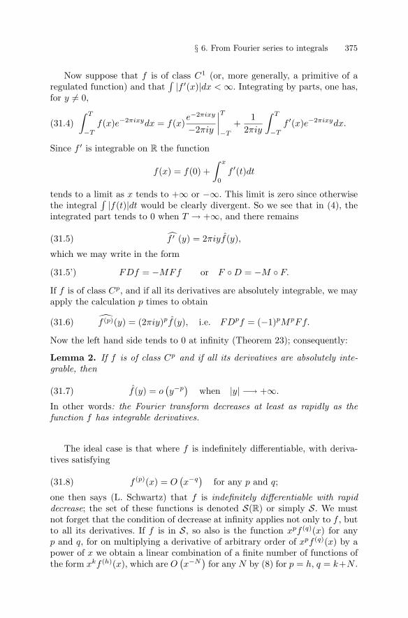
§ 6. From Fourier series to integrals 375
Now suppose that f is of class C1 (or, more generally, a primitive of aregulated function) and that
∫ |f ′(x)|dx < ∞. Integrating by parts, one has,for y �= 0,∫ T
−T
f(x)e−2πixydx = f(x)e−2πixy
−2πiy
∣∣∣∣T−T
+1
2πiy
∫ T
−T
f ′(x)e−2πixydx.(31.4)
Since f ′ is integrable on R the function
f(x) = f(0) +∫ x
0
f ′(t)dt
tends to a limit as x tends to +∞ or −∞. This limit is zero since otherwisethe integral
∫ |f(t)|dt would be clearly divergent. So we see that in (4), theintegrated part tends to 0 when T → +∞, and there remains
f ′ (y) = 2πiyf(y),(31.5)
which we may write in the form
FDf = −MFf or F ◦ D = −M ◦ F.(31.5’)
If f is of class Cp, and if all its derivatives are absolutely integrable, we mayapply the calculation p times to obtain
f (p)(y) = (2πiy)pf(y), i.e. FDpf = (−1)pMpFf.(31.6)
Now the left hand side tends to 0 at infinity (Theorem 23); consequently:
Lemma 2. If f is of class Cp and if all its derivatives are absolutely inte-grable, then
f(y) = o(y−p)
when |y| −→ +∞.(31.7)
In other words: the Fourier transform decreases at least as rapidly as thefunction f has integrable derivatives.
The ideal case is that where f is indefinitely differentiable, with deriva-tives satisfying
f (p)(x) = O(x−q)
for any p and q;(31.8)
one then says (L. Schwartz) that f is indefinitely differentiable with rapiddecrease; the set of these functions is denoted S(R) or simply S. We mustnot forget that the condition of decrease at infinity applies not only to f , butto all its derivatives. If f is in S, so also is the function xpf (q)(x) for anyp and q, for on multiplying a derivative of arbitrary order of xpf (q)(x) by apower of x we obtain a linear combination of a finite number of functions ofthe form xkf (h)(x), which are O
(x−N)
for any N by (8) for p = h, q = k+N .
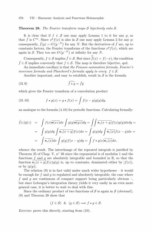
376 VII – Harmonic Analysis and Functions Holomorphic
Theorem 28. The Fourier transform maps S bijectively onto S.
It is clear that if f ∈ S one may apply Lemma 1 to it for any p, sothat f is C∞. Since xpf(x) is also in S one may apply Lemma 2 for any p;consequently, f(y) = O
(y−N)
for any N . But the derivatives of f are, up toconstants factors, the Fourier transforms of the functions xpf(x), which areagain in S. They too are O
(y−N)
at infinity for any N .
Consequently, f ∈ S implies f ∈ S. But since f(x) = f(−x), the conditionf ∈ S implies conversely that f ∈ S. The map is therefore bijective, qed.
An immediate corollary is that the Poisson summation formula, Fourier’sinversion formula and Plancherel’s formula apply to every f ∈ S.
Another important, and easy to establish, result in S is the formula
f � g = f g(31.9)
which gives the Fourier transform of a convolution product
f � g(x) = g � f(x) =∫
f(x − y)g(y)dy,(31.10)
an analogue to the formula (4.10) for periodic functions. Calculating formally:
f(z)g(z) =∫
f(x)e(xz)dx
∫g(y)e(yz)dy =
∫ ∫ez(x + y)f(x)g(y)dxdy =
=∫
g(y)dy
∫ez(x + y)f(x)dx =
∫g(y)dy
∫ez(x)f(x − y)dx =
=∫
ez(x)dx
∫g(y)f(x − y)dy =
∫f � g(x)ez(x)dx,
whence the result. The interchange of the repeated integrals is justified byTheorem 25 of Chap. V, n◦ 26 since the exponential is of modulus 1 and thefunctions f and g are absolutely integrable and bounded in R, so that thefunction ez(x + y)f(x)g(y) is, up to constants, dominated either by |f(x)|,or by |g(y)|.
The relation (9) is in fact valid under much wider hypotheses – it wouldbe enough for f and g to regulated and absolutely integrable, the case wheref and g are continuous of compact support being particularly obvious –,but since Lebesgue’s integration theory yields it very easily in an even moregeneral case, it is better to wait to deal with this.
Since the ordinary product of two functions of S is again in S (obvious!),(9) and Theorem 28 show that
(f ∈ S) & (g ∈ S) =⇒ f � g ∈ S.
Exercise: prove this directly, starting from (10).
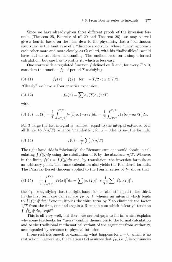
§ 6. From Fourier series to integrals 377
Since we have already given three different proofs of the inversion for-mula (Theorem 25, Exercise of n◦ 29 and Theorem 26), we may as wellgive a fourth, based on the idea, dear to the physicists, that a “continuousspectrum” is the limit case of a “discrete spectrum” whose “lines” approacheach other more and more closely, as Cavalieri, with his “indivisibles”, wouldhave had no trouble understanding. The method rests on a simple formalcalculation, but one has to justify it, which is less easy.
One starts with a regulated function f defined on R and, for every T > 0,considers the function fT of period T satisfying
fT (x) = f(x) for − T/2 < x ≤ T/2.(31.11)
“Clearly” we have a Fourier series expansion
fT (x) =∑
an(T )en(x/T )(31.12)
with
an(T ) =1T
∫ T/2
−T/2
fT (x)en(−x/T )dx =1T
∫ T/2
−T/2
f(x)e(−nx/T )dx.(31.13)
For T large the last integral is “almost” equal to the integral extended overall R, i.e. to f(n/T ), whence “manifestly”, for x = 0 let us say, the formula
f(0) ≈ 1T
∑f(n/T ).(31.14)
The right hand side is “obviously” the Riemann sum one would obtain in cal-culating
∫f(y)dy using the subdivision of R by the abscissae n/T . Whence,
in the limit, f(0) =∫
f(y)dy and, by translation, the inversion formula atan arbitrary point. The same calculation also yields the Plancherel formula.The Parseval-Bessel theorem applied to the Fourier series of fT shows that
1T
∫ T/2
−T/2
|fT (x)|2dx =∑
|an(T )|2 ≈ 1T 2
∑|f(n/T )|2,(31.15)
the sign ≈ signifying that the right hand side is “almost” equal to the third.In the first term one can replace fT by f , whence an integral which tendsto∫ |f(x)|2dx; if one multiplies the third term by T to eliminate the factor
1/T from the first, one finds again a Riemann sum which “clearly” tends to∫ |f(y)|2dy, “cqfd”.This is all very well, but there are several gaps to fill in, which explains
why some textbooks for “users” confine themselves to the formal calculationand to the traditional mathematical variant of the argument from authority,accompanied by recourse to physical intuition.
If one restricts oneself to examining what happens for x = 0, which is norestriction in generality, the relation (12) assumes that fT , i.e. f , is continuous
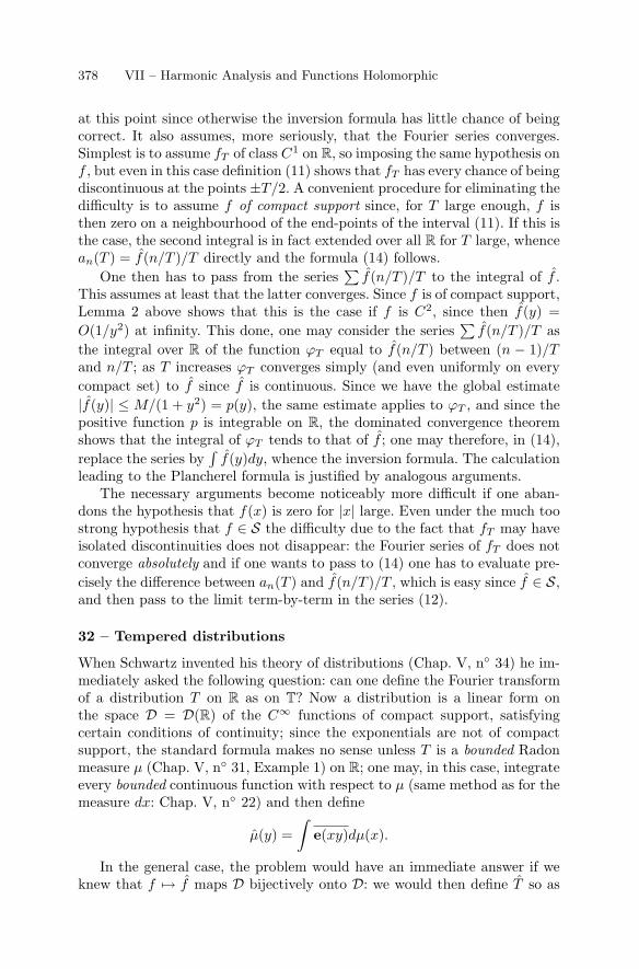
378 VII – Harmonic Analysis and Functions Holomorphic
at this point since otherwise the inversion formula has little chance of beingcorrect. It also assumes, more seriously, that the Fourier series converges.Simplest is to assume fT of class C1 on R, so imposing the same hypothesis onf , but even in this case definition (11) shows that fT has every chance of beingdiscontinuous at the points ±T/2. A convenient procedure for eliminating thedifficulty is to assume f of compact support since, for T large enough, f isthen zero on a neighbourhood of the end-points of the interval (11). If this isthe case, the second integral is in fact extended over all R for T large, whencean(T ) = f(n/T )/T directly and the formula (14) follows.
One then has to pass from the series∑
f(n/T )/T to the integral of f .This assumes at least that the latter converges. Since f is of compact support,Lemma 2 above shows that this is the case if f is C2, since then f(y) =O(1/y2) at infinity. This done, one may consider the series
∑f(n/T )/T as
the integral over R of the function ϕT equal to f(n/T ) between (n − 1)/Tand n/T ; as T increases ϕT converges simply (and even uniformly on everycompact set) to f since f is continuous. Since we have the global estimate|f(y)| ≤ M/(1 + y2) = p(y), the same estimate applies to ϕT , and since thepositive function p is integrable on R, the dominated convergence theoremshows that the integral of ϕT tends to that of f ; one may therefore, in (14),replace the series by
∫f(y)dy, whence the inversion formula. The calculation
leading to the Plancherel formula is justified by analogous arguments.The necessary arguments become noticeably more difficult if one aban-
dons the hypothesis that f(x) is zero for |x| large. Even under the much toostrong hypothesis that f ∈ S the difficulty due to the fact that fT may haveisolated discontinuities does not disappear: the Fourier series of fT does notconverge absolutely and if one wants to pass to (14) one has to evaluate pre-cisely the difference between an(T ) and f(n/T )/T , which is easy since f ∈ S,and then pass to the limit term-by-term in the series (12).
32 – Tempered distributions
When Schwartz invented his theory of distributions (Chap. V, n◦ 34) he im-mediately asked the following question: can one define the Fourier transformof a distribution T on R as on T? Now a distribution is a linear form onthe space D = D(R) of the C∞ functions of compact support, satisfyingcertain conditions of continuity; since the exponentials are not of compactsupport, the standard formula makes no sense unless T is a bounded Radonmeasure µ (Chap. V, n◦ 31, Example 1) on R; one may, in this case, integrateevery bounded continuous function with respect to µ (same method as for themeasure dx: Chap. V, n◦ 22) and then define
µ(y) =∫
e(xy)dµ(x).
In the general case, the problem would have an immediate answer if weknew that f → f maps D bijectively onto D: we would then define T so as
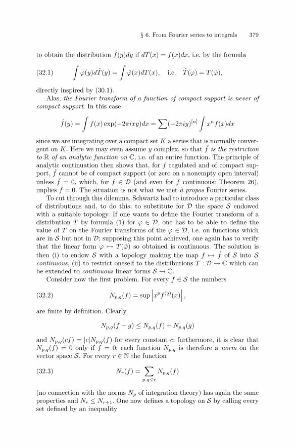
§ 6. From Fourier series to integrals 379
to obtain the distribution f(y)dy if dT (x) = f(x)dx, i.e. by the formula∫ϕ(y)dT (y) =
∫ϕ(x)dT (x), i.e. T (ϕ) = T (ϕ),(32.1)
directly inspired by (30.1).Alas, the Fourier transform of a function of compact support is never of
compact support. In this case
f(y) =∫
f(x) exp(−2πixy)dx =∑
(−2πiy)[n]
∫xnf(x)dx
since we are integrating over a compact set K a series that is normally conver-gent on K. Here we may even assume y complex, so that f is the restrictionto R of an analytic function on C, i.e. of an entire function. The principle ofanalytic continuation then shows that, for f regulated and of compact sup-port, f cannot be of compact support (or zero on a nonempty open interval)unless f = 0, which, for f ∈ D (and even for f continuous: Theorem 26),implies f = 0. The situation is not what we met a propos Fourier series.
To cut through this dilemma, Schwartz had to introduce a particular classof distributions and, to do this, to substitute for D the space S endowedwith a suitable topology. If one wants to define the Fourier transform of adistribution T by formula (1) for ϕ ∈ D, one has to be able to define thevalue of T on the Fourier transforms of the ϕ ∈ D, i.e. on functions whichare in S but not in D; supposing this point achieved, one again has to verifythat the linear form ϕ → T (ϕ) so obtained is continuous. The solution isthen (i) to endow S with a topology making the map f → f of S into Scontinuous, (ii) to restrict oneself to the distributions T : D → C which canbe extended to continuous linear forms S → C.
Consider now the first problem. For every f ∈ S the numbers
Np,q(f) = sup∣∣∣xpf (q)(x)
∣∣∣ ,(32.2)
are finite by definition. Clearly
Np,q(f + g) ≤ Np,q(f) + Np,q(g)
and Np,q(cf) = |c|Np,q(f) for every constant c; furthermore, it is clear thatNp,q(f) = 0 only if f = 0; each function Np,q is therefore a norm on thevector space S. For every r ∈ N the function
Nr(f) =∑
p,q≤r
Np,q(f)(32.3)
(no connection with the norms Np of integration theory) has again the sameproperties and Nr ≤ Nr+1. One now defines a topology on S by calling everyset defined by an inequality
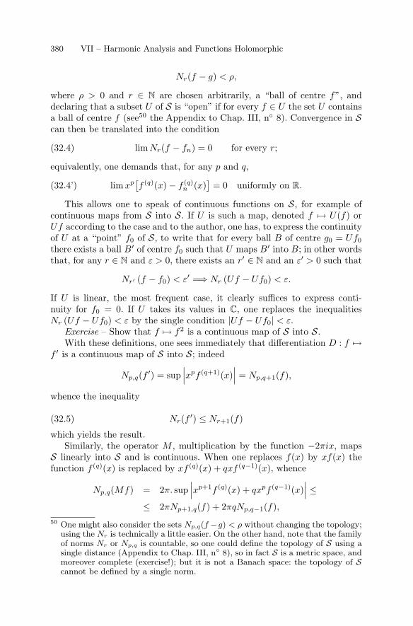
380 VII – Harmonic Analysis and Functions Holomorphic
Nr(f − g) < ρ,
where ρ > 0 and r ∈ N are chosen arbitrarily, a “ball of centre f”, anddeclaring that a subset U of S is “open” if for every f ∈ U the set U containsa ball of centre f (see50 the Appendix to Chap. III, n◦ 8). Convergence in Scan then be translated into the condition
limNr(f − fn) = 0 for every r;(32.4)
equivalently, one demands that, for any p and q,
limxp[f (q)(x) − f (q)
n (x)]
= 0 uniformly on R.(32.4’)
This allows one to speak of continuous functions on S, for example ofcontinuous maps from S into S. If U is such a map, denoted f → U(f) orUf according to the case and to the author, one has, to express the continuityof U at a “point” f0 of S, to write that for every ball B of centre g0 = Uf0
there exists a ball B′ of centre f0 such that U maps B′ into B; in other wordsthat, for any r ∈ N and ε > 0, there exists an r′ ∈ N and an ε′ > 0 such that
Nr′ (f − f0) < ε′ =⇒ Nr (Uf − Uf0) < ε.
If U is linear, the most frequent case, it clearly suffices to express conti-nuity for f0 = 0. If U takes its values in C, one replaces the inequalitiesNr (Uf − Uf0) < ε by the single condition |Uf − Uf0| < ε.
Exercise – Show that f → f2 is a continuous map of S into S.With these definitions, one sees immediately that differentiation D : f →
f ′ is a continuous map of S into S; indeed
Np,q(f ′) = sup∣∣∣xpf (q+1)(x)
∣∣∣ = Np,q+1(f),
whence the inequality
Nr(f ′) ≤ Nr+1(f)(32.5)
which yields the result.Similarly, the operator M , multiplication by the function −2πix, maps
S linearly into S and is continuous. When one replaces f(x) by xf(x) thefunction f (q)(x) is replaced by xf (q)(x) + qxf (q−1)(x), whence
Np,q(Mf) = 2π. sup∣∣∣xp+1f (q)(x) + qxpf (q−1)(x)
∣∣∣ ≤≤ 2πNp+1,q(f) + 2πqNp,q−1(f),
50 One might also consider the sets Np,q(f −g) < ρ without changing the topology;using the Nr is technically a little easier. On the other hand, note that the familyof norms Nr or Np,q is countable, so one could define the topology of S using asingle distance (Appendix to Chap. III, n◦ 8), so in fact S is a metric space, andmoreover complete (exercise!); but it is not a Banach space: the topology of Scannot be defined by a single norm.
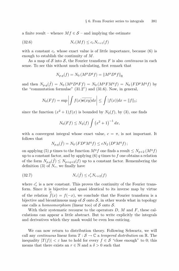
§ 6. From Fourier series to integrals 381
a finite result – whence Mf ∈ S – and implying the estimate
Nr(Mf) ≤ crNr+1(f)(32.6)
with a constant cr whose exact value is of little importance, because (6) isenough to establish the continuity of M .
As a map of S into S, the Fourier transform F is also continuous in eachsense. To see this without much calculating, first remark that
Np,q(f) = N0 (MpDqf) = ‖MpDqf‖R
and then Np,q(f) = N0 (MpDqFf) = N0 (MpFMqf) = N0 (FDpMqf) bythe “commutation formulae” (31.2”) and (31.6). Now, in general,
N0(Ff) = sup∣∣∣∣∫
f(x)e(xy)dx
∣∣∣∣ ≤∫
|f(x)|dx = ‖f‖1;
since the function (x2 + 1)f(x) is bounded by N2(f), by (3), one finds
N0(Ff) ≤ N2(f)∫ (
x2 + 1)−1
dx,
with a convergent integral whose exact value, c = π, is not important. Itfollows that
Np,q(f) = N0 (FDpMqf) ≤ cN2 (DpMqf) ;
on applying (5) p times to the function Mqf one finds a result ≤ Np+2 (Mqf)up to a constant factor, and by applying (6) q times to f one obtains a relationof the form Np,q(f) ≤ Np+q+2(f) up to a constant factor. Remembering thedefinition (3) of Nr, we finally have
Nr(f) ≤ c′rNr+2(f)(32.7)
where c′r is a new constant. This proves the continuity of the Fourier trans-form. Since it is bijective and quasi identical to its inverse map by virtue
of the relation f(x) = f(−x), we conclude that the Fourier transform is abijective and bicontinuous map of S onto S, in other words what in topologyone calls a homeomorphism (linear too) of S onto S.
With their systematic recourse to the operators D, M and F , these cal-culations can appear a little abstract. But to write explicitly the integralsand derivatives which they mask would be even less enticing.
We can now return to distribution theory. Following Schwartz, we willcall any continuous linear form T : S → C a tempered distribution on R. Theinequality |T (f)| < ε has to hold for every f ∈ S “close enough” to 0; thismeans that there exists an r ∈ N and a δ > 0 such that
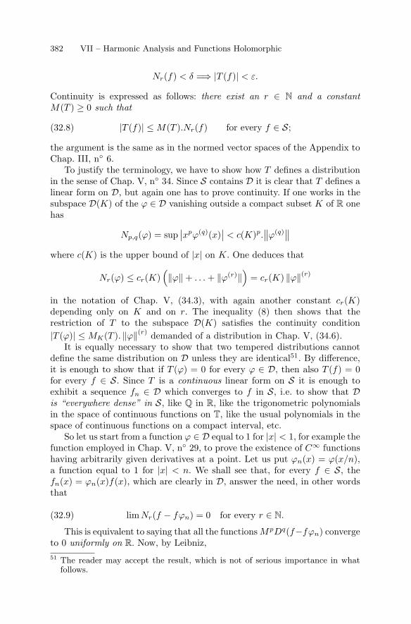
382 VII – Harmonic Analysis and Functions Holomorphic
Nr(f) < δ =⇒ |T (f)| < ε.
Continuity is expressed as follows: there exist an r ∈ N and a constantM(T ) ≥ 0 such that
|T (f)| ≤ M(T ).Nr(f) for every f ∈ S;(32.8)
the argument is the same as in the normed vector spaces of the Appendix toChap. III, n◦ 6.
To justify the terminology, we have to show how T defines a distributionin the sense of Chap. V, n◦ 34. Since S contains D it is clear that T defines alinear form on D, but again one has to prove continuity. If one works in thesubspace D(K) of the ϕ ∈ D vanishing outside a compact subset K of R onehas
Np,q(ϕ) = sup∣∣xpϕ(q)(x)
∣∣ < c(K)p.∥∥ϕ(q)∥∥
where c(K) is the upper bound of |x| on K. One deduces that
Nr(ϕ) ≤ cr(K)(‖ϕ‖ + . . . + ‖ϕ(r)‖
)= cr(K) ‖ϕ‖(r)
in the notation of Chap. V, (34.3), with again another constant cr(K)depending only on K and on r. The inequality (8) then shows that therestriction of T to the subspace D(K) satisfies the continuity condition|T (ϕ)| ≤ MK(T ). ‖ϕ‖(r) demanded of a distribution in Chap. V, (34.6).
It is equally necessary to show that two tempered distributions cannotdefine the same distribution on D unless they are identical51. By difference,it is enough to show that if T (ϕ) = 0 for every ϕ ∈ D, then also T (f) = 0for every f ∈ S. Since T is a continuous linear form on S it is enough toexhibit a sequence fn ∈ D which converges to f in S, i.e. to show that Dis “everywhere dense” in S, like Q in R, like the trigonometric polynomialsin the space of continuous functions on T, like the usual polynomials in thespace of continuous functions on a compact interval, etc.
So let us start from a function ϕ ∈ D equal to 1 for |x| < 1, for example thefunction employed in Chap. V, n◦ 29, to prove the existence of C∞ functionshaving arbitrarily given derivatives at a point. Let us put ϕn(x) = ϕ(x/n),a function equal to 1 for |x| < n. We shall see that, for every f ∈ S, thefn(x) = ϕn(x)f(x), which are clearly in D, answer the need, in other wordsthat
limNr(f − fϕn) = 0 for every r ∈ N.(32.9)
This is equivalent to saying that all the functions MpDq(f−fϕn) convergeto 0 uniformly on R. Now, by Leibniz,51 The reader may accept the result, which is not of serious importance in what
follows.
§ 6. From Fourier series to integrals 383
MpDq(f − fϕn) = Mp [Dqf − (Dqf.ϕn + . . . + f.Dqϕn)](32.10)= Mp (1 − ϕn) Dqf − Mp(. . .)
where the terms inside the sign (. . .) contain derivatives of ϕn, i.e. functionsof the form n−kϕ(k)(x/n) with 1 ≤ k ≤ q. Such a function is everywherebounded in modulus by n−k
∥∥Dkϕ∥∥, so that the sum of the terms considered
is, for every x, bounded in modulus by∑1≤k≤q
?n−k∥∥Dkϕ∥∥ . ∣∣Dq−kf(x)
∣∣ ;the signs ? denote binomial coefficients of no importance. If one applies theoperator Mp of multiplication by (−2πix)p to these terms one obtains afunction ∑
?n−k∥∥Dkϕ∥∥ . ∣∣xpDq−kf(x)
∣∣with other coefficients ? independent of f and of n. In passing to the sup forx ∈ R one finds a result less than∑
?n−k∥∥Dkϕ∥∥ .Nr(f)
where r = p+q. Since the sum is over the k ∈ [1, q] and since n−k ≤ 1/n, thefinal result, up to a constant factor independent of ϕ and of r, is bounded byNr(f)/n. For f given, it is therefore O(1/n).
It remains to examine the term Mp (1 − ϕn) Dqf in (10). Since ϕn(x) = 1for |x| < n, this term vanishes for |x| < n. Ignoring the factors −2πi, itsuniform norm on R is then in fact equal to
sup|x|>n
|1 − ϕn(x)| . |xpDqf(x)| .
Now |1 − ϕn(x)| ≤ 1+‖ϕ‖ = c. Since f ∈ S the function∣∣xp+1Dqf(x)
∣∣ tendsto 0 at infinity, so is bounded on R; we deduce estimates of the form
|xpDqf(x)| ≤ cpq/|x|valid for every x ∈ R. The sup for |x| > n is thus, also, O(1/n).
Combining these two results, we see that
‖MpDq (f − fϕn)‖ = O(1/n)
for any p and q, which proves that f = lim fϕn in the topology of S, qed.
This done, it is immediate to define the Fourier transform T = FT of atempered distribution T : one puts, in Leibniz’ notation,∫
f(y)dT (y) =∫
f(x)dT (x)(32.11)
384 VII – Harmonic Analysis and Functions Holomorphic
or, in that of the inventor,
T (f) = T (f) for every f ∈ S.(32.11’)
Since the map f → f of S in S is continuous, so likewise is f → T (f), andso is f → T (f), whence one obtains a tempered distribution.
One may also, as in Chap. V, n◦ 35, define the derivative – again tempered– of T by
T ′(f) = −T (f ′) for every f ∈ S,(32.12)
and iterate the operation. To calculate the derivative DT of T one has towrite
DT (f) = −T (Df) = −T (FDf)
where F is the Fourier transform in S; but (31.5’) shows that FDf = −MFf ;thus
DT (f) = T (MFf).(32.13)
Putting DT = S, this can be written∫f(x)dS(x) =
∫(−2πiy)f(y)dT (y) = −
∫f(y)2πiydT (y).
Thus we see the distribution “of density 2πiy with respect to dT (y)” appear;if T were of the form p(y)dy with a reasonable function p we would thusobtain the distribution −2πiyp(y)dy. So it is natural to write MT for thedistribution −2πiydT (y), the ordinary product of T by the function −2πiy;it is again given by52
MT (f) = T (Mf) for every f ∈ S.(32.14)
This done, (13) can be written
DFT (f) = MT (Ff) = FMT (f)(32.15)
by definition of the Fourier transform FMT of MT . In other words, the for-mula DF = FM remains valid for tempered distributions. One can showsimilarly that MFT = −FDT : the Fourier transform exchanges the op-erators of differentiation and of multiplication by −2πix in the context offunctions or of distributions.52 The formula has a meaning only because multiplication by 2πiy maps S con-
tinuously into S. One may define p(y)dT (y) for every function p which is C∞
and such that f �→ pf maps S into S. This assumes that p and its successivederivatives do not increase more rapidly at infinity than powers of x (“temperedfunctions”): the product of a function “of slow increase” by a function “of rapiddecrease” is again of rapid decrease.
§ 6. From Fourier series to integrals 385
If for example f is a regulated function which is O( |x|N ) at infinity for an
integer N > 0, then the formula
Tf (ϕ) =∫
ϕ(x)f(x)dx
has a meaning for every ϕ ∈ S and defines a tempered distribution; its Fouriertransform is, by definition, the Fourier transform of f ; it goes without sayingthat it is not a function in general.
In particular let us take f(x) = xp with p ∈ N. Then
Tf (ϕ) = Tf (ϕ) =∫
ϕ(y)ypdy for ϕ ∈ S;
multiplying by (−2πi)p, one makes the function MpFϕ = (−1)pFDpϕ ap-pear in the integral. Then
(2πi)pTf (ϕ) =
∫FDpϕ(y)dy.
But since Dpϕ is in S we may apply the Fourier inversion formula to it,whence
(2πi)pTf (ϕ) = Dpϕ(0) = δ (Dpϕ) ,
where δ is the Dirac measure at the origin, clearly a tempered distribution.In view of definition (12) of the derivative of a distribution, the result can bewritten
(2πi)pTf = δ(p),
the derivative of order p of the distribution δ. For p = 0, we see that theFourier transform of the function 1 is the Dirac measure at the origin: this isexactly what formula f(0) =
∫f(y)dy, valid for f ∈ S, means.
In conclusion we remark that all this generalises to functions of severalvariables. See for example the excellent Chap. 3 of Michael E. Taylor, PartialDifferential Equations. Basic Theory (Springer, 1996) or the ultracondensedexposition of Lars Hormander, The Analysis of Linear Partial DifferentialEquations, Vol. 1 (Springer, 1983).
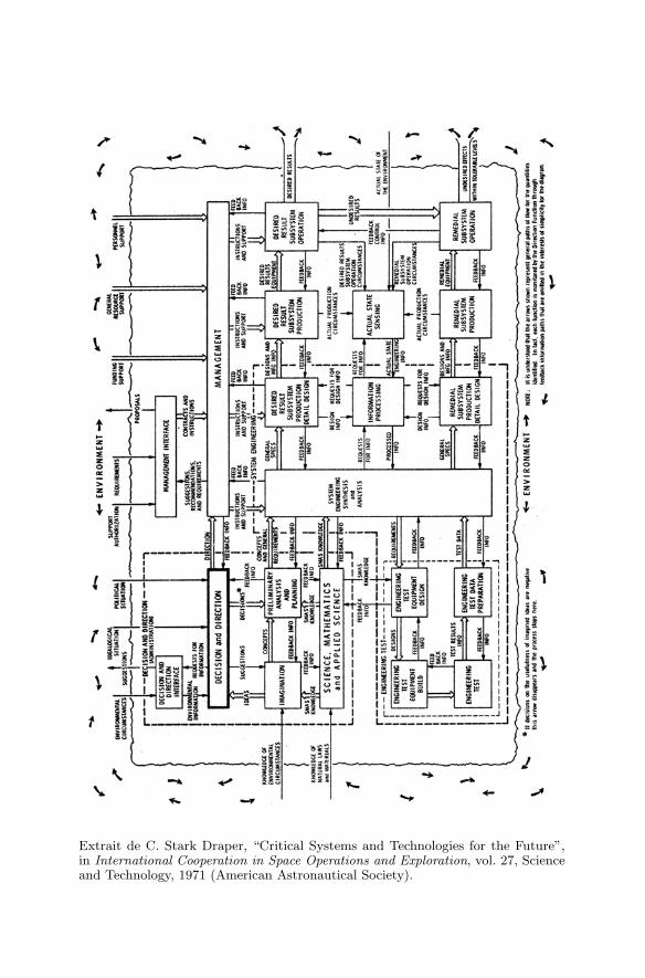
Extrait de C. Stark Draper, “Critical Systems and Technologies for the Future”,in International Cooperation in Space Operations and Exploration, vol. 27, Scienceand Technology, 1971 (American Astronautical Society).
Postface
Science, technology, arms
The text below is only a part of the postface that was announced in thepreface to volume I; the full text, with references to sources, is substantiallylonger than the French version, already 90 pages long. It will be available tointerested readers on the Internet, at the following address:
www.springer.online.com/de/3-540-20921-2Readers who wish to understand why a mathematics textbook includes thetext below will find explanations in the preface to volume I.
I have tried to be as pedagogical as possible, but since this postface dealswith many topics far removed from mathematics, it will, of course, requiresome work and good will from the reader to understand it.
Many sources have been used, and all of them will be found in the internetversion. A few have been mentioned in the printed text.
Italics have been used for verbatim quotations in the main text.
§ 1. How to fool young innocents
The H-bomb was born in September 1941 at Columbia University in NewYork during a conversation between Enrico Fermi and Edward Teller. Theexplosion of an atomic bomb based on the fission of U-235 or Pu-239 nucleicould generate the tens or hundreds of million degrees necessary for the fusionof hydrogen nuclei, which in turn would generate amounts of energy hundredsof times greater than that of the atomic bomb itself. This was nothing morethan a very rough idea, but Teller and others already knew (or believed) by1942 that, if a 30 kg mass of U-235
is used to detonate a surrounding mass of 400 kg of liquid deu-terium, the destructiveness should be equivalent to that of more than10,000,000 tons of TNT [the standard military explosive]. This shoulddevastate an area of more than 100 square miles.
Yet the development of the A-bombs which destroyed Hiroshima (U-235) andNagasaki (Pu) was top priority during the war, so that nothing much hap-pened for several years although a few people around Teller continued theirtheoretical studies of the problem; after a team of physicists reviewed theissues in the spring of 1946, even Teller went back to theoretical physics at
388 Postface
Chicago. Calculations were very difficult to carry out, they neglected phys-ical effects that opposed the fusion reaction, the choice of which isotopesof hydrogen to fuse was not easy, and the geometrical configurations theywere drawing up could not work or, if they did, could not lead to the ul-timate weapon, namely something with theoretically unlimited power. Lastbut not least, experimental verification of the computations was impossibleshort of exploding an actual weapon. In addition, many influential physicistswere against the development of a weapon which they viewed as being fartoo powerful and which would most likely be imitated by the Soviet Unionsooner or later.
The situation changed dramatically after the announcement in September1949 by President Harry Truman of a first secret (but detected) Soviet atomictest. The General Advisory Committee (GAC) of the Atomic Energy Com-mission (AEC, now part of the Department of Energy, DoE) was convenedto deal with the new situation at the end of October. Basically for ethi-cal reasons, the GAC members (scientists J. Robert Oppenheimer, ArthurCompton, James Conant, Enrico Fermi, Lee A. DuBridge, Isidor I. Rabi,Cyril Stanley Smith, as well as the Bell Labs president, Oliver E. Buckley,and Hartley Rowe, an engineer) were unanimous in their opposition to thedevelopment and production of the H-bomb, though they were not againstfurther theoretical studies; they recommended the production of more fissionbombs – new types under development, up to 500 kilotons (KT), were deemedpowerful enough to deter the Soviets -, including “tactical” ones (for use inEurope...), and they recommended providing by example some limitation onthe totality of war; when briefed by Oppenheimer, the tough Secretary ofState, Dean Acheson, a friend and admirer, replied: How can you persuade aparanoid adversary to disarm “by example” ? Other scientists, like Teller andErnest Lawrence who were not GAC members, were also strongly in favorand briefed the president of the Congressional Committee on Atomic Energyand top men in the Air Force, who began to call for it. Three of the AECadministrators (including the AEC President) were against it, and the othertwo for it, including Lewis Strauss, a most influential and conservative WallStreet tycoon who, like Teller, was as “paranoid” as Joe Stalin, and did nothesitate to go straight to Truman. The H-bomb supporters rejected the ideathat America might come out second in the H-bomb race; and in an Americaagain made fiercely anti- Communist by the Soviet domination of EasternEurope, by the 1948 attempt to blockade Berlin, and by the “loss” of Chinato the Communists in 1949, the overwhelming majority of people also wantedsupremacy over, not parity with, the Soviet Union. Furthermore, the near to-tal American demobilization in 1945 and the rejection of Universal MilitaryTraining meant that reliance on atomic weapons was America’s only meansof deterring, slowing down, or resisting the onrush of a Red Army which,after demobilizing, still retained about three million men and compulsory
Postface 389
military training, even though the said onrush was considered by people inthe know to be quite improbable within five years.
As President Truman said at the time, there was actually no decision tomake on the H-bomb: he shared these arguments and, at the end of January1950, after three months of totally secret discussions involving about onehundred people, he publicly announced that the development of the H-bombwould continue; he also forbade people connected with the AEC, includingGAC members, to discuss the subject in public.
In early February, thanks to the partial decrypting of Soviet wartimetelegrams, the unfolding of the Fuchs affair in Britain a few days earlierproved that the bright ex-German Communist physicist sent by the Britishto Los Alamos in 1943 had transmitted to the Soviets not only essential dataon the A-bomb, but also most probably what was known on the future H-bomb up to April 1946: he had even taken a patent out on it, in commonwith von Neumann! The Soviets thus knew America was on the H-bomb trail,and America knew that the Soviets might also be working on it, as Tellerhad claimed – rightly, but without proof – long before. In March 1950, onthe advice of the military, who did not need this new piece of information tomake up their minds, Truman, this time secretly, made H-bomb productiona top priority.
The correct physical principles were not even known. Numerical calcula-tions carried out by mathematicians John von Neumann at Princeton andStanislas Ulam at Los Alamos, and performed partly on the new but insuffi-ciently powerful electronic machines, confirmed that Teller’s ideas could notlead to the weapon he had been dreaming of since 1942; Teller’s optimisticcalculations still relied on incorrect hypotheses or missing data. One (the-oretical) version of the weapon under consideration in 1950, which woulddevelop a power of the order of 1,000 megatons, was some 30 feet long, anda stunning 162 feet wide; the fission trigger alone weighed 30,000 pounds.Technical follies, as Freeman Dyson would later say.
Anyway, developing the weapon had to be done at the Los Alamos lab-oratory where the A-bomb had been developed and where a reduced teamhad remained or had been recruited since Hiroshima. Although the outbreakof the Korean war led many top physicists to join the project, many mem-bers were on Oppenheimer’s side as Teller knew full well, and he believedthey were not enthusiastic enough to succeed. Supported again by ErnestLawrence, the Air Force, and key Congressmen, Teller asked for the creationof a rival laboratory in 1950, but his request was denied by the Atomic En-ergy Commission. Teller was desperate at the end of 1950 and no longer surea true H-bomb, with arbitrary large power, could be made.
But in January 1951, Ulam devised a new geometric configuration: toseparate completely the atomic triggerfrom the material to be fused. It wasseized by Teller who found an entirely new way to make the fusion workbefore the bomb blew up: the near-solid wave of neutrons flowing from the
390 Postface
atomic explosion was too slow; instead, his idea was to use the X-ray burstfrom it to generate the necessary temperature and pressure. During a meetingat the Princeton Institute for Advanced Research (which Oppenheimer nowheaded) in June 1951, everyone enthusiastically agreed that this was thesolution, and Teller got the laboratory he had asked for in September 1952.In November 1952, a test of the principles, using liquid deuterium and a goodsized refrigeration installation, produced the 10 megatons (MT) predicted in1942; it also vaporized a small island in the Pacific ocean. In April 1954,several tests of near-operational weapons using lithium deuteride, an easilystored white powder, produced between 10 and 15 MT – two or three timesmore than predicted, because one of the reaction phases had been overlooked.Operational weapons (10-15 MT) went aboard giant B-36 bombers from theend of 1954 to 1957; later ones never exceeded 5 MT and most were in thehundreds of KT range. All of these successes, and the great majority of laterachievements too, were the work of Los Alamos people “lacking enthusiasm”.The first true Soviet H-bomb was tested in November 1955 and producedabout 1.6 megatons.
Set up at Livermore, not far from Berkeley, Teller’s laboratory is nowcalled the Lawrence Livermore Laboratory (LLL) and has been managed, atleast officially, by the University of California since 1952, as Los Alamos hasbeen since 1943. All American nuclear weapons were invented at these twoplaces; while this still remains Los Alamos’ basic activity, Livermore later con-centrated a large part of its work on much more innovative scientific-militaryprojects, as will be seen below. Lawrence won a Nobel prize for his inven-tion at Berkeley in the 1930s of the first particle accelerators (cyclotrons).To a large extent, this was made possible by philanthropists attracted bythe potential medical uses of radiation or artificial radio-elements availablemuch more cheaply and abundantly than radium. During the war, Lawrenceinitiated and headed a massive electromagnetic isotope-separation processinspired by his cyclotrons; you can gauge Lawrence’s influence from the factthat the Treasury Department lent him over thirteen thousand tons of silverto wire his “calutrons”, despite an endless series of unexpected technical prob-lems which brought operations to a complete halt as soon as the war ended.They nevertheless performed the final enrichment, at 80% of U-235, of muchof the partly enriched uranium obtained from another massive factory, whereuranium hexafluoride – a very nasty gas – was blown through thousands ofporous metallic “barriers”; the very primitive Hiroshima bomb used some 60kg of the final product. Together with Oppenheimer, Fermi, Arthur Comp-ton and Conant, as well as the Secretaries of War and State, Lawrence hadparticipated in the June 1945 top- level discussions concerning the use ofthe first available bombs. They had also recommended a well-financed re-search program in nuclear physics, military and civilian applications, as wellas weapons production.
Postface 391
It was to this most influential operator, whose Berkeley Rad Lab hadstrong connections with Los Alamos, that the Atomic Energy Commissionentrusted in 1952 the task of setting up a new development center for the H-bomb. Livermore needed a director, and Lawrence chose one of his assistants,Herbert York, then 30 years old.
After Sputnik (1957), York took charge for a while of all American mili-tary research and development. Health problems forced him to cut down onhis activities, and he “retired” to a California university, while still partici-pating in negotiations and meetings on arms control. From 1970 on, he wrotearticles and books about the arms race, the absurdity and danger of whichhe could now clearly see.
In 1976 he wrote a short book, The Advisors, recounting the developmentof the thermonuclear project and, in particular, the discussions which hadtaken place at the end of 1949 on the opportunity to launch a H-bomb devel-opment program. His book reproduces in full the recently declassified reportin which the AEC’s General Advisory Committee explains the practical andethical reasons against it.
With a rare frankness, York discloses the reasons which led him to par-ticipate in the project after the start of the Korean War (which led some op-ponents of the H-bomb, like Fermi and Bethe, to change their minds). Therewas first the growing seriousness of the cold war, much influenced by my veryclose student-teacher relationship with Lawrence, a fierce anti-Communist likeTeller, Ulam, and von Neumann. There was also the scientific and technicalchallenge of the experiment itself: it’s not every day you get the opportunityto explode the equivalent of ten million tons of TNT for the first time inhistory (it was actually done by Los Alamos). There was also, and perhapsmost importantly as every young scientist can understand,
my discovery that Teller, Bethe, Fermi, von Neumann, Wheeler,Gamow, and others like them were at Los Alamos and involved inthis project. They were among the greatest men of contemporaryscience, they were the legendary yet living heroes of young physi-cists like myself, and I was greatly attracted by the opportunity ofworking with them and coming to know them personally.
Moreover,
I was not cleared to see GAC documents or deliberations, and so Iknew nothing about the arguments opposing the superbomb, exceptfor what I learned second hand from Teller and Lawrence who, ofcourse, regarded these arguments as wrong and foolish. (I saw theGAC report for the first time in 1974, a quarter of a century later!)
In less than one page, you have something similar to the corruption of aminor taking place in the scientific milieu: you are told that the enemy isthreatening your country, the scientific problem is fascinating, great menyou admire set the example, other great men you don’t know personally are
392 Postface
opposed to the project but their arguments are top secret, those great menwho are luring you carefully refrain from honestly telling you what thesearguments are, and, anyway, you’ll be able to read the official documents in25 or 30 years if you are American, in 50 or 60 if you are French or British,and, at the earliest, after the fall of the regime if you are a Soviet citizen. Ifyou are still alive, your delayed comments will have no impact whatsoeverbecause the project in which you participated was completed decades before,and its justifications have perhaps changed radically in the meantime.
This had already been seen in the A-bomb project: physicists were told (orclaimed) in 1941 that the A-bomb was needed before the Nazis got one, it wasdiscovered in May 1945, if not before, that they were years behind, but thebombs were still dropped: over a thoroughly defeated Japan. Quite a numberof participants felt they had been fooled, even though they did not know,as we now do, that three weeks after Hiroshima, the Air Force sent GeneralGroves, head of the Manhattan Project, a list of two dozen Soviet cities andasked him to provide the weapons (which was not done until 1948), whileStalin was giving absolute priority to his own atomic project. And nobodythen – except perhaps Groves – imagined that tens of thousands of bombswould eventually be produced.
Main references: Herbert York, The Advisors. Oppenheimer, Teller,and the Superbomb (Freeman, 1976), Stanislas Ulam, Adventures ofa Mathematician (Scribner’s, 1976), Richard Rhodes, The Makingof the Atomic Bomb (Simon & Schuster, 1988) and Dark Sun. TheMaking of the Hydrogen Bomb (Simon & Schuster, 1995), GreggHerken, Brotherhood of the Bomb. The Tangled Lives and Loyal-ties of Robert Oppenheimer, Ernest Lawrence, and Edward Teller(Henry Holt, 2002), Peter Goodchild, Edward Teller. The Real Dr.Strangelove (Harvard UP, 2004), David C. Cassidy, Oppenheimer andthe American Century (PI Press, 2005).
York may not have been alone in this kind of situation; as Gordon Dean,AEC president 1950-1954, said at the Oppenheimer security hearing in 1954:
We were recruiting men for that laboratory [Livermore], I would saypractically all of whom came immediately out of school. They wereyoung Ph.D.’s and some not Ph.D.’s (...) Under Lawrence’s adminis-tration, with Teller as the idea man, with York as the man who wouldpick up the ideas and a whole raft of young imaginative fellows youhad a laboratory working entirely – entirely – on thermonuclear work.
Livermore’s then two divisions (thermonuclear and fission) were headed byHarold Brown, then 24, and John Foster, then 29; they both were later tohead Livermore, then all military R&D, and even the Department of Defense(DoD). I don’t know whether, once past the age of innocence, some of these“young imaginative fellows” reflected on their past as York did.
Postface 393
I do know of other similar cases though. Theodore B. Taylor (1925-2004),on hearing about Hiroshima, vowed never to have anything to do with atomicweapons, but he studied physics. In 1948, believing he was working for peace,he joined Los Alamos where he developed a fascination and a gift for improv-ing atomic weapons. He invented the best A-weapons of the time, including a500 KT fission weapon which, in May 1951, succeeded in fusing a few gramsof deuterium; he also became an expert in predicting the effects of nuclearweapons. He left in 1956 for General Atomic (founded by one of Teller’s col-leagues) and the design of nuclear reactors, then headed the development ofa spaceship propelled by multiple small atomic explosions and able to sendpeople to Mars and beyond – the Nuclear Test Ban treaty prohibiting at-mospheric tests killed that project in 1963; in 1964 he was put in charge ofthe maintenance of nuclear weapons, in 1966 he resigned and worked for awhile with the international Vienna agency (AIEA) responsible for control-ling the civilian nuclear energy business. His initial taste for weapons turnedinto its very opposite, notably after a visit to Moscow when, looking at thecrowd in Red Square, he remembered he had helped the Air Force select theweapons best adapted to targets around the city, the Kremlin being mostprobably number one on the list. He spent the rest of his life advocating theabolition of nuclear weapons and nuclear energy which, he believed, wouldlead to an uncontrollable proliferation of weapons and even to their use byterrorists, a prospect he predicted in 1970 by emphasizing that the WorldTrade Center building could easily be felled by a small atomic explosion onits ground floor.
Recruiting young imaginative fellows at Livermore and other places is stillgoing on, of course. William Broad, a New York Times science journalist whospent a week there in 1984 with a very special “O group” of young physiciststwenty to thirty years old, explains in Star Warriors the role of the HertzFoundation, founded shortly after Sputnik by Hertz Rent-a-Car’s patrioticowner in order to maintain US technological preponderance (and to showhis gratitude to a country which turned a poor immigrant into a very richman). Every year the Foundation allocates about twenty five fellowships,valid for five years, to outstanding students; some of these are invited tospend a summer (or several years) at Livermore while preparing for theirPh.D. elsewhere. Those Broad met were asked to put their energies intoproblems at the cutting edge of technology with a not so obvious militaryinterest: to build an optical computer using laser lines instead of electricalconnections, to design from scratch and to miniaturize a supercomputer,to devise an X-ray laser, to elaborate a credible model of an atomic bombusing only published literature, etc. The group leader, Lowell Wood (whostill sits on the Foundation Board together with several other Livermore orLos Alamos people), explained that:
The best graduate students tend to do very marvelous work becauseit’s a win-or-die situation for them. There is no graceful second place.
394 Postface
If somebody else publishes the definitive results in the area, they goback to zero and start over (...) They don’t realize how extremelychallenging these problems are. So they are not dismayed or demor-alized at first. By the time they begin to sense how difficult theproblems are, they’ve got their teeth into them and made sufficientprogress so that they tend to keep going. Most of them win. Theyoccasionally lose, which is very sad to see (p. 31).
One of them, Peter Hagelstein, remembers his arrival in Teller’s kingdom in1975 when he was 20 years old:
The lab itself made quite an impression, especially the guards andbarbed wire. When I got to the personnel department it dawned onme [!] that they worked on weapons here, and that’s about the firstI knew about it. I came pretty close to leaving. I didn’t want to haveanything to do with it [and his girlfriend was militantly opposedto it, which eventually destroyed their relationship]. Anyway, I metnice people, so I stayed. The people were extremely interesting. AndI really didn’t have anywhere else to go.
Hagelstein was asked to study the X-ray laser. He first spent four years, at therate of 80-100 hours a week, learning the physics and doing computations witha very powerful program of his own. A senior Livermore physicist, GeorgeChapline, had been trying for years to find a solution by using a nuclearexplosion to get the energy needed to “pump” the laser (it is proportional tothe cube of the frequency, which for X-rays is about 1000 times that of visiblelight). A first underground test in September 1978 was a failure because ofa leak in a vacuum line. On Thanksgiving Day 1978, some senior physicists– including Wood, Chapline and an unwilling Hagelstein – were summonedto Teller’s home to discuss the problem; Hagelstein was ordered by Teller toreview the calculations done for Chapline – nothing more, but nothing less– and he had no choice but to comply. By the next day, he had to tell Woodthere was a flaw in Chapline’s theory, which put him in direct competitionwith Chapline. He found new ideas which he once dropped at a meeting in1979, too tired after a 20-hour working day to realize what he was doing. Theywere seized upon at once and, he told Broad, he had [his] arm twisted to doa detailed calculation , under political pressures like you wouldn’t believe . Tohis despair and with some prodding from Wood and Teller, his calculationsand new ideas proved more and more promising, and in 1980 an undergroundtest of his and Chapline’s new designs proved Hagelstein’s method was byfar the better. He then had access to Livermore’s gigantic laser lines, and hislaser, though still virtual, got a name: Excalibur.
Hagelstein tells us of political pressures; no wonder. On the political side,for several years before Reagan’s election, some very influential people – theCommittee on the Present Danger – had been claiming that the Soviets werespending far more on defense than even the CIA said, and were re-arming
Postface 395
to full capacity. As a matter of fact, since 1975 they had been deployinga few hundred new strategic missiles with multiple independent warheads(MIRV) (deployment of 840 American Minuteman-III MIRV missiles, and of640 Poseidon submarine-launched similar missiles, had started in 1970 and1971, respectively). They were also deploying very accurate middle-range SS-20s aimed at strategic targets in Western Europe and China. Their output ofbasic industrial goods (steel, coal, cement, etc.) was 50 to 100% higher thanAmerica’s (but the American economy was converting to an “informationsociety” far more efficient than Stalin’s successors’ taste for steel). They werediscovering huge fields of oil and natural gas from which they got plenty offoreign currency, allowing them to buy (mostly American) grain and, muchworse, advanced foreign machinery in spite of the US embargo on high-techgoods. “Marxists” were seizing power in several African states; unrest inPoland was repressed by the Polish army to avoid a Soviet intervention; theRed Army had intervened (unwillingly at first) in Afghanistan to defendthe new Communist regime against its enemies, which many interpreted asa first Soviet step towards the proverbial Persian Gulf “warm waters” theTsars had never managed to seize. The American deployment in Europe ofequally dangerous American Pershing ballistic missiles and Tomahawk cruisemissiles in answer to the SS-20s was opposed by strong “peace movements”that were suspected of being infiltrated by Soviet agents since, of course,ordinary German citizens were deemed too stupid to worry for themselvesabout these displays of atomic fire power. In short, the world had enteredwhat became known as the New Cold War .
Thirty two members of the Committee on the Present Danger, includingReagan, occupied high administration offices after he came to the WhiteHouse in January 1981. He immediately started to re-arm – the DoD budget,mostly financed by foreign capital attracted by high interest rates, went upfrom 181 BD in 1978 to 270 in 1984 in constant dollars -, and he continued totaunt the Soviets in speeches that culminated in his famous “Evil Empire”statement in 1983. However, many people in Washington, including Reaganhimself, believed that in spite of its apparent strength, the USSR was undertremendous economic pressure with a grossly inflated military sector and agrossly underdeveloped civilian sector. They thought that a new round in thearms race would bankrupt the Soviets, or force them to agree to significantcuts in strategic armaments, or both.
There were already people in America trying to sell untested and wildanti-missile schemes, e.g. chemical lasers, 24 of which could supposedly de-stroy an entire fleet of Soviet missiles, or thousands of interceptors launchedfrom hundreds of space stations. This led another bunch of conservative busi-nessmen who had nothing to do with nuclear weapons, but were close to Rea-gan, to found a High Frontier committee, including Teller who wanted to sellhis X-ray laser right away; they wanted to reach the White House without go-ing through the Pentagon bureaucracy, where hard technical questions would
396 Postface
be asked, of course. In this way, Teller was able to recommend a Los Alamosfriend as Scientific Advisor, George Keyworth, who in turn appointed himto the new White House Science Council. A High Frontier report was sentto Reagan, and they got a fifteen-minute audience in January 1982; Tellerapparently did not attend. They claimed that the Russians were well aheadin technology (as Teller had claimed to promote his H-bomb project), thatthey were close to deploying directed-energy weapons in space, thus alteringthe world balance of power. They recommended that America launch a majorprogram to counter the Soviet threat in order to substitute assured survivalfor assured destruction , which suited Reagan quite well. Hagelstein’s X-raylaser was the key to success and would be available within four years, followedby even more powerful versions. All of this rested on the secret results of asingle test performed in a totally artificial underground environment.
Reagan, however, asked Keyworth to gather a team of experts from hisScience Council in order to review the project before the end of 1982, ifonly to get an idea of the price tag. During this year, peace movementsin America and Europe drew hundreds of thousands of people (and manyscientists) demonstrating against the new arms race; many American Con-gressmen agreed. In June, a group of Livermore scientists who had the re-sponsibility of continuing work after the first test, reported that the projectwould require ten more tests, six years, and 150-200 million a year to es-tablish reliably that this laser was scientifically possible; it would then haveto be transformed into an operational space weapon, which would requirestill more engineering, money, and years. This made Teller furious and allthe more convinced that, as had been the case with the H-bomb, the projectneeded a lot of hype to take off. After complaining on TV that he had notyet met with President Reagan, he got an audience in September; some ofthose present interjected so many questions that Teller (and Keyworth) feltthe meeting had been a disaster. In December, the House rejected funds forthe production of a new and widely criticized generation of missiles, the MX,which could be randomly moved underground among many silos, most ofthem empty, in order to fool the Russian MIRV missiles. In January 1983,Teller got an audience with the Chief of Naval Operations; he was convincedby Teller’s views and converted the Joint Chiefs of Staff; to them, it was atleast a way of convincing Moscow of the sheer financial power and technicalsuperiority of the US , as well as a new way to inflate the Defense budget sinceMX was becoming far too controversial. A meeting with Reagan in February1984 ended in agreement; the military believed this would lead to an orderlydevelopment project, but Reagan did not wait. In March, to everyone’s as-tonishment, he publicly announced his Strategic Defense Initiative (SDI, orStar Wars) project designed to protect the American people from Soviet mis-siles – a popular statement if ever there was one, which nevertheless did notplacate the opposition.
Postface 397
In the meantime, in February 1983, a most famous nuclear physicist, HansBethe, had gone to Livermore, reviewed Hagelstein’s project and found it ex-tremely clever physics, which did not mean clever weaponry. After Reaganlaunched his Star Wars project, Hagelstein’s laser became the most publi-cized – and controversial – part of it though it was still, at best, years awayfrom any kind of operational status; a second test in March was actuallyinconclusive due to a recording failure. The media explained that, propelledinto space by a single missile, individually oriented towards enemy missiles,and “pumped” by a nuclear explosion, fifty X-ray lasers were expected todestroy as many targets. Many physicists, foremost among them Hans Betheand Richard Garwin, were opposed to this new exotic hardware display andsaid so publicly, because the chances of success were poor for many reasons –the need for fantastically fast computers and communications (laser weaponswould be launched from submarines after the Soviet attack was detected,they would have to spot missiles moving at a speed of four miles per secondand then orient the laser rods before firing, etc.) -, because nobody knewwhether the project would cost 150 or 3,000 billion dollars (BD) if successful,and because it would only lead to one more spiral in the arms race and/orcould be easily defeated (as the Soviets at once remarked). Another officialpanel reviewing the project came to rather pessimistic conclusions, relegat-ing Reagan’s dream to the year 2000 or so, and calling for a less ambitiousgoal, while at the same time recommending one billion and top priority forthe laser, and 26 billion over seven years for the various other projects: SDIhad already acquired an immense political power by this time. During a pro-paganda tour of Europe in 1985(?), SDI chief, General James Abrahamsonused plenty of sexy slides to explain it all at the Paris Ecole polytechnique (Iattended); this was a major contribution to the students’ scientific education:they (and I) did not know a thing about X-ray lasers, but you can trust themto have “understood” everything within a week.
A few days after a successful test in December 1983, Teller sent anoverly optimistic report to Keyworth, without notifying anyone, not even RoyWoodruff, a senior Livermore physicist who was deputy director for weaponsdesign and thus oversaw the X-ray laser group; Woodruff was furious andwrote a corrective letter, which was blocked by Livermore’s director. In theSpring of 1984, other objections arose. According to Los Alamos scientists,beryllium mirrors that were sending a fraction of the beam to recording in-struments contained oxygen which, excited by the beam, possibly increasedthe recorded brightness. The dispersion of the laser beam in space, the num-ber of space stations and the power of the explosions needed were also publiclycriticized by independent scientists. But in Washington others noticed thatSoviet negotiators – who had been working for years on arms reduction –were very concerned about this militarization of space and therefore mightbe more accommodating, others again thought SDI would be a good oppor-
398 Postface
tunity to wreck the 1972 ABM treaty which seriously limited the deploymentof anti-ballistic missiles.
By 1984, Hagelstein had lost his initial dislike for weapons:
My view of weapons has changed. Until 1980 or so I didn’t wantto have anything to do with nuclear anything. Back in those days Ithought there was something fundamentally evil with weapons. NowI see it as an interesting physics problem.
He did not have any illusions:
I’m more or less convinced that one of these days we’ll have WorldWar III or whatever. It’ll be pretty ugly. A lot of cities will get bustedup.
In October 1984, Hagelstein and a team of forty people realized at long lastthe first “laboratory” X-ray laser, using a 150-meter long laser line pumpedby capacitors discharging ten billion watts; this success was still very far fromthe operational weapon Teller was promising Reagan.
During this time, the Livermore group had devised the theoretical meansto increase the laser power by several orders of magnitude, so that now“Super-Excalibur” lasers could be placed on a stationary orbit and still beable to kill missiles 20,000 miles away! At the end of 1984, Teller wrotethrough Wood to Paul Nitze, since 1950 the top expert in arms-control ne-gotiations:
a single X-ray laser module the size of an executive desk which ap-plied this technology could potentially shoot down the entire Sovietland-based missile force, if it were to be launched into the module’sfield of view.
Woodruff was again by-passed but learned of the letter; he again tried tosend a corrective one, which again was blocked. However, in February 1985,he was allowed a two- hour meeting with Nitze, who said that it’s alwaysgood to get a bright skeptical mind on a problem . The initial results of anew and very elaborate test seemed so good in March that Teller’s constantlobbying did pay off: hundreds of millions were released.
That same month, Mikhail Gorbachev came to power in the USSR, witha quasi-revolutionary program to transform the Soviet Union into a near-democracy and to terminate the arms race and the Cold War, which Reaganwanted too (but by other means). Although his scientists told him that SDIcould be neutralized for 10% of the price to America, he decided to focusthe US-Soviet arms-control talks on removing SDI in exchange for heavycuts in missiles. Reagan met him in Geneva in November 1985 and, althoughthe meeting was rather friendly, Gorbachev told him he should not counton bankrupting the Soviet Union or achieving military predominance, andthat SDI would render impossible the expected 50% reduction in missiles.Reagan replied by extolling the virtues of defense, as usual. They continued
Postface 399
to correspond for months in the hope of getting some kind of agreement;many of Reagan’s aides and top military (not to mention Europeans, in-cluding France’s president Mitterand) were appalled by Reagan’s apparentwillingness to dump American missiles provided he could keep SDI.
In October, at the annual conference of Los Alamos and Livermore peopleon nuclear weapons, Los Alamos scientists reiterated in detail their skepticismover the test results or even the existence of the X-ray laser; this allowed mostmembers of the X-ray laser group to understand for the first time that theseobjections were serious. And Los Alamos people accused Livermore managersof abdicating their prerogatives to Teller and Wood, who, of course, claimedLos Alamos were trying to sabotage their project for political reasons or out ofrivalry. This was enough for Woodruff, who resigned from his position. Teller’spredictions, however, became somewhat more careful, and he emphasizedthat defense would be efficient even if it were only 20% effective becauseenough US missiles would survive to deter the Soviets attacking in the firstplace.
In November, a new and very expensive test (30 MD) resulted mostly infailure. Some Livermore scientists, who were already exasperated by Wood’sauthoritarian and sarcastic manner and by Teller’s constant meddling in theirwork, left the project; as one of them said in 1989,
To lie to the public, because we know that the public doesn’t under-stand all this technical stuff, brings us down to the level of hawkersof snake oil, miracle cleaners and Veg-O-Matics.
Although he dismissed Los Alamos objections, Hagelstein too was disgustedby Teller’s and Wood’s extravagant public claims and by the bad faith themain protagonists displayed; as he told Goodschild in 2000, I could not believepeople behaved in that way . However, it is easy to understand why they did.These people with plenty of willpower had for decades been in charge ofdesigning the awesome weapons on which US security was supposed to rest.They were under enormous political pressure, and billions of dollars hadalready been spent on or budgeted for their pet project. Their reputationsand the laboratory’s were at stake.
Hagelstein quit Livermore for the MIT Research Laboratory in Electron-ics, which had been conducting military research since 1945, and worked inquantum electronics and, later, “cold fusion”. This is a very controversial andto this day unproven method of generating energy at room temperature bymeans of fusion reactions among metallic compounds of hydrogen and deu-terium. His scientific reputation suffered greatly as a result. As to Woodruff,he was exiled to a tiny office (“Gorky West”) and his salary cut for sev-eral years, a good illustration of the contradicting ethics governing open andclassified research; he joined Los Alamos in 1990.
The conflict between the two laboratories surfaced in the newspapers, trig-gering another public but inconclusive discussion, since the relevant technicaldata were top secret. In 1986 several thousand scientists publicly pledged not
400 Postface
to participate in SDI in spite of the promise of exciting problems to solveand plenty of money for their laboratories. Politically, Teller won; he wassupported by the military, by influential Congressmen, and by Reagan whounderstood nothing but trusted the “father of the H-bomb”; Teller hesitatedneither to rely on Reagan’s faith, nor to use his own scientific self-confidence,reputation and authority to ruthlessly counter opponents.
As for the Star Wars project, it survived until Bill Clinton’s election in1992. In January 1986, Gorbachev proposed to get rid of all Euromissiles onboth sides, and to eliminate all nuclear weapons by 2000, provided Americagave up developing, testing and deploying space weapons. Reagan proposedinstead to reduce strategic warheads to 6,000 on each side (this was achievedfour years later under George Bush) and to redress existing conventional im-balances. In July, Reagan proposed scrapping all ballistic missiles within tenyears while continuing research on SDI which, when operational, would bemade available to all (!). They had a second meeting in Reykjavik in Oc-tober 1986 during which extraordinary proposals were made on both sideswith a view to eliminating nuclear weapons entirely and reducing conven-tional forces. Once more, SDI killed the agreement at the last moment. Gor-bachev’s advisors (who were as bewildered as their American counterpartsby these proposals) told him that Congress would kill SDI for him anyway.He did not follow their advice, but they were right: Congress cut the SDIbudget by one third and prohibited tests in space in December 1987. In themeantime, a Livermore friend of Teller’s had found a new miracle weapon,Brilliant Pebbles : space stations firing thousands of sophisticated projec-tiles, full of electronics, which would collide with Soviet warheads. A thirdReagan-Gorbachev meeting in Washington a few weeks later led to the endof Euromissiles.
The Cold War died in 1990 and with it the Soviet Union and SDI; a fewyears later, the French Riviera was invaded by a new brand of Bolsheviks:oligarchs. The life expectancy of ordinary Russians began to decline. TheEuropean Union eastern boundaries (and with it those of NATO, a clever wayof assuaging nationalist feelings in Russia) are now the pre-1939 boundariesof the former USSR. Last but not least, it has been “proved” that socialismis a dead end (especially if confronted with savage aggression followed by aruinous fifty-year arms race led by a far more powerful opponent).
When asked why SDI did not work, Teller recently replied with a shrug:because the technology was not ready. The X-ray laser had cost 2.2 BD, andStar Wars a total of 30 BD. America is now spending a mere ten billion ayear to develop anti-missile weapons against lesser threats than the Sovietarsenal, while Livermore (as well as the French Atomic Energy Commission)is trying to achieve, among other projects, controlled nuclear fusion of hydro-gen isotopes by means of convergent laser beams in the hope, going back to1950, of transforming nuclear fusion into an inexhaustible source of energy,as was done much earlier with nuclear fission. This also allows weapons de-
Postface 401
signers to gain a deeper knowledge of fusion processes so as to improve theircomputer programs.
Main references: William J. Broad, Star Warriors. The Weaponryof Space: Reagan’s Young Scientists (Simon and Schuster, 1985 orFaber and Faber, 1986), Goodchild, Edward Teller , Martin Walker,The Cold War (Vintage, 1994), John Prados, The Soviet Estimate.US Intelligence Analysis and Soviet Strategic Forces (Princeton UP,1986), Stephen I. Schwartz, ed., Atomic Audit. The Costs and Con-sequences of US Nuclear Weapons Since 1940 (Brookings, 1998).
Before having a look at Ken Alibek’s Soviet career in biological weapons(BWs) from 1975 to the fall of the Soviet Union, let me sketch their previ-ous development. After Pasteur, Koch, Metchnikoff and others had foundedmicrobiology, it became possible to produce large amounts of vaccines. Italso became obvious that, if required, similar techniques could be used tocultivate pathogens. That it was not pure theory was shown when the 1925Geneva Convention prohibited it. The USA did not sign it, but the USSRand Japan did; it seems that USSR began to develop a typhus weapon in1928, while Japan installed a very successful secret laboratory and produc-tion unit in Manchuria in the 1930s. Britain started to study vaccines after1936 and, after the Nazis had advertized their brand of ethics at Warsaw andRotterdam, thought it advisable to develop BWs as a hedge against similarGerman ones (they were not studied seriously until 1943 and came to almostnothing). British scientists worked mainly with anthrax, a bacterium whichis easy to cultivate and store by transforming into spores that stay virulentfor decades. Conclusive experiments on sheep were done at Gruinard Island,off Scotland; it was still contaminated and off limits fifty years later. Theymade anthrax cakes in sufficient quantities to be able to kill a lot of Germancattle (and some people as well).
In America, studies on BWs began in 1940, and a National Academy ofSciences (NAS) committee was set up a month before Pearl Harbor. Althoughits February 1942 report was inconclusive in the absence of practical tests, itrecommended studying all possibilities (for defense, of course) including an-thrax, botulin toxin, and cholera. The program involved the Chemical War-fare Service, the Department of Agriculture for anti-crops weapons, and 28universities. Although behind Britain until Pearl Harbor, American industryquickly developed a far bigger military potential than Britain, which, in thisdomain as in others (atomic bomb, radar, jet engines, etc.), contributed ex-perts and knowledge, including penicillin which was industrialized in Americaduring the war.
A research center was set up at Camp Detrick and, in Vigo, Indiana,a factory equipped with twelve 5,000-gallon fermenters could in principleproduce 500,000 four-pound anthrax bombs a month, or 250,000 filled withbotulin toxin (lethal dose: one milligram). The Americans also investigatedbrucellosis, a more humane weapon which kills few people, but is highly
402 Postface
contagious and makes its victims ill for weeks or months, thus overwhelmingthe enemy’s health system. Weapons for use against Japanese rice crops werealso developed. But Roosevelt was not very interested in these matters aboutwhich he was very ill informed, and he never made his position clear one wayor the other.
In any case, peace came before this program became operational, andVigo was leased to a private manufacturer of penicillin. In 1945 BWs wereconsidered potentially at least as efficient as, and much cheaper than, theatomic bomb; and since they don’t destroy real estate, you don’t have tocompensate the enemy and allies after the victory. But atomic weapons wereviewed as a sufficient deterrent, performing realistic tests of BWs was im-possible, and the new German neurotoxic gases (tabun, sarin, soman) killedmuch faster – in a few minutes – than BWs. So, at first, work on BWs waslimited to laboratory studies. During the Korean War, the Americans wereaccused of having experimented with BWs; it is now generally believed theyhad not, but the war accelerated the arms race in all domains, includingBWs. In both the US and the USSR, all kinds of bacteria – anthrax, plague,tularemia, yellow fever -, and later viruses, were studied and mass produced.From 1947, the Soviets worked on smallpox which, by now eradicated, wasstill killing some 15 million people a year in the world in the 1960s. They builthuge research centers and production units, some in cities, such as Sverdlovsk.The CIA had reason to suspect the worst as U-2 and satellite observationsshowed installations looking very much like the American ones, for instancea test range on an island in the Aral Sea.
During the 1950s, scientists in both countries discovered that instead ofstoring or spreading bacteria as liquid cultures, it was far better to dry anddeep-freeze them (lyophilization); this kept them dormant for long periods,even at room temperature. The result was then milled into an ultra-finepowder which, after being carried by the wind over possibly tens of miles,became virulent again in people’s lungs. This process worked particularly wellwith anthrax, the pulmonary form of which is normally rare and difficult todiagnose and kills 90% of its victims unless they are administered massivedoses of penicillin very early.
The “top secret” American programs were actually known to plenty ofpeople and, like the use of chemicals to destroy jungles in Vietnam, met withopposition from journalists, students, and biologists like Harvard’s MatthewMeselson and Joshua Lederberg; the latter, who won a 1958 Nobel prize forhis discovery of how bacteria can exchange genes in a natural setting, was ina good position to know that fast progressing molecular biology can be bentto genocide , as he wrote in the Washington Post in 1968. During the Viet-nam war, opponents, particularly students, organized public demonstrationsagainst Fort Detrick, as well as protests against military- university contractsand the National Academy of Sciences’ involvement in recruiting young sci-entists for Fort Detrick. For their part, the military were not yet convinced of
Postface 403
the usefulness of these weapons; proliferation was too easy and too cheap, andterrorist attacks were already being mentioned. Eventually, President Nixonunilaterally announced in November 1969 that America would limit herselfto purely defensive work, and he ordered the destruction of stocks and thedemilitarization of Fort Detrick, Pine Bluff and other centers; I remember aScience headline: Is Fort Detrick really de-tricked ? In 1972, an internationaltreaty between the US, the USSR and Britain, later approved by many othercountries, prohibited the production and possession of biological weapons,but not defensive laboratory work; it did not provide for inspections either.
Before 1972, and although “weaponizing” pathogens required solving diffi-cult technical problems, only natural bacteria and viruses were used. In 1972-1973, American biologists succeeded in systematically moving a gene from anorganism to a bacterium in such a way that the modified bacterium wouldreplicate itself as usual; their first experiment yielded a variant of the nor-mally harmless Escherichia Coli that was resistant to penicillin. Thus geneticengineering was born and, with it, the possibility of discovering, by chance oron purpose, new pathogens from which no protection was known. But in theUSSR, molecular biology and Mendelian genetics had been almost destroyedby Lysenko in the 1930s, and Soviet scientists were increasingly frustrated atthe thought of being left behind. According to Alibek, the situation changedwhen a vice president of the Akademia Nauk, Yuri Ovchinnikov, explainedto the Ministry of Defense and to President Brezhnev that bioengineeringcould lead to new weapons.
This led to the founding in 1973 of an officially civilian pharmaceuticalorganization, Biopreparat, under the Ministry of Health. Biopreparat’s openmission was to develop and produce standard vaccines and antibiotics, but itenclosed a supersecret “Enzyme” project whose purpose was to develop andproduce for intercontinental war genetically altered pathogens, resistant toantibiotics and vaccines , an outright violation of the 1972 treaty. It also led,as Ovchinnikov hoped, to a reversal of the taboo against genetics and mole-cular biology, and to new laboratories depending on the Moscow Academysince “purely scientific” work was paramount for “defense” against biologi-cal weapons. The timing was perfect: gene splicing had just been discovered,and its practical importance would soon be proved in the USA by using engi-neered bacteria to produce large amounts of insulin, hormones, etc. Enzyme,which was led by military scientists and administrators with KGB men every-where, came to employ 32,000 workers, including many of the best biologists,epidemiologists, and biochemists, in addition to thousands of people workingin Army labs.
Let us now go back to Alibek. Hoping to become a military physicianwho could save soldiers on the battlefields, he studied medicine at a militaryschool and became interested in research. In 1973, he was ordered by oneof his teachers to investigate a very unusual outbreak of tularemia whichoccurred around Stalingrad in 1942 among German troops before spreading
404 Postface
to the Soviet army. After reading old documents, Alibek reported that thisincident looked as though it had been caused intentionally . He was at oncecut short by his teacher who told him he was only supposed to describe howwe handled the outbreak , not what had caused it, and strongly advised neverto mention to anyone else what you just told me. Believe me, you’ll be doingyourself a favor . The lessons he drew from this episode are worth quoting:
The moral argument for using any available weapon against an enemythreatening us with certain annihilation seemed to me irrefutable. Icame away from this assignment fascinated by the notion that diseasecould be used as an instrument of war. I began to read everything Icould find about epidemiology and the biological sciences.
In 1975, a mysterious and well tailored visitor came to interview him andother students; he said he was working for a no less mysterious organizationattached to the Council of Ministers which has something to do with biologicaldefense , a prospect which excited Alibek. He was handed a questionnaireand told: Don’t tell your friends or teachers about this conversation. Not evenyour parents . A few weeks later, he learned he was assigned to the Councilof Ministers of the Soviet Union together with four other students. He wasoverjoyed by the prospect of working in Moscow, but he was actually sentto a “post office box” hundreds of miles from Moscow. Like Hagelstein, hewas impressed by the concrete wall and barbed wire surrounding the placeand by the armed guards at the entrance. The huge Omutninsk Base wherehe arrived already employed some 10,000 people; it was part of the Enzymeproject.
On arrival at Omutninsk, Alibek and his friends were not given any infor-mation about their research program. A KGB instructor however informedthem that although an international treaty banning biological weapons hadbeen signed in 1972, it was obviously one more American hoax , which theywere quite prepared to believe; the Soviet Union therefore had to be readyto reply.
When Alibek began to discover Omutninsk’s true mission – mass pro-duction of pathogens and not merely laboratory research -, he tried to getanother job but was told he could not be spared. He thus remained and,after this classic early conscience crisis, adapted to the situation with enoughsuccess and enthusiasm to become Biopreparat’s deputy director fifteen yearslater. The science and technique were fascinating and the career very reward-ing provided you were bright, which he was, and made no big mistakes (suchas inoculating yourself or being too talkative...).
The new recruits were trained in the culture of bacteria, the techniques be-ing the same whether they are intended for industrial applications, weaponiza-tion, or vaccination . This is a difficult art which is first learned on harmlessbacteria; one then has to learn how to infect lab animals with mildly patho-genic agents and conduct autopsies, until one may perhaps be allowed towork in “hot zones” with infected animals and where wearing the equivalent
Postface 405
of a space suit is compulsory: half a dozen Ebola viruses will kill you in amonth by destroying your blood vessels. A very competent colleague of Al-ibek once made a false move while inoculating an animal; after his death,they noticed the viruses in his body were particularly virulent, and there-fore they weaponized this “Ustinov strain”. One also has to learn industrialproduction processes.
Smallpox was modified to render all known vaccines useless. Diphtheriawas grafted on plague. Sergei Popov, a bright colleague, improved Legionnellawith fragments of myelin DNA to trigger metabolic reactions that devastatethe brain and nervous system. The invention of a form of tularemia resis-tant to three of the main antibiotics, as well as studies on Ebola-like virusestook years of work. All in all, little produced by the genetic engineering pro-grams was turned into weapons before the Soviet Union collapsed, accordingto Popov who has been living in the USA since 1992; Alibek also remainssomewhat skeptical, though more pessimistic.
Incidents happened during this period. In April 1979, about sixty peopledied within a few weeks in the city of Sverdlovsk, an extremely unusualevent. There was a Biopreparat branch located in the city, working roundthe clock on anthrax. A Russian magazine in West Germany broke the newsof the outbreak in November, from which US intelligence agents again drewconclusions, despite claims that the deaths were due to contaminated meat.It is now known that a clogged air filter had been removed but not replacedfor several hours...
In October 1989, Vladimir Pasechnik, a very bright scientist at the headof a civilian institute in Leningrad, went to France at the invitation of apharmaceutical equipment manufacturer, and never came back. Since hisinstitute had worked very efficiently for Biopreparat, he knew quite a lot. Hewas brought to Britain and debriefed.
Pasechnik’s defection had serious consequences. In a memo to Gorbachev,KGB chairman Vladimir Kryuchkov recommended the liquidation of our bi-ological weapons production lines , a stunning move which Alibek approvedsince, after all, so long as we had the strains in our vaults, we were only threeto four months away from full capacity . Although many powerful peopledisapproved of Kryuchkov’s initiative, Gorbachev issued a few weeks later asecret decree, prepared by Alibek and another fellow, ordering Biopreparatto cease to function as an offensive warfare agency ; but in transmittingAlibek’s text to the Kremlin, his chief added a paragraph instructing theorganization to keep all of its facilities prepared for further manufacture anddevelopment , which resurrected Biopreparat as a war organization, as Alibeksays. He was furious but this, at any rate, allowed him to order an end tomilitary development at some of the most important installations.
A second consequence was an agreement between the USA, UK and theUSSR to organize inspections of suspected BW facilities. The first inspectionof a few Biopreparat installations took place in January 1991; Alibek and
406 Postface
the Russian side were very successful in showing as little as possible, but thevisitors, who were aware of Pasechnik’s disclosures, were not fooled.
In December 1991, during the week the Soviet Union collapsed, a visitto four American installations chosen by the Russians took place; they wereknown to anybody who had read Science magazine around 1970 (as I did).The Russian team included Alibek who could verify that these installationswere in a dilapidated condition that precluded military work, or had beenconverted to medical research – work on the rejection of organ transplantsfascinated the Russians -, or, in one case, had never done any military re-search. The Soviet delegation nevertheless reported to the contrary, and thisconvinced Alibek that official justifications for his work had been a KGBhoax rather than an American one.
He resigned from the Army, then from Biopreparat, got a job at oncein a bank – I had no aptitude for finance, but I was soon making deals likeeveryone else -, and went on business trips abroad. His telephone was tapped,police watched him around Moscow, and some associates warned him that hehad better not leave Russia for good and that in any case his family wouldnever get permission to leave. In the meantime, a Yeltsin decree banned alloffensive research and cut defense funding.
Alibek then went back to his native Kazakhstan, a newly independentcountry where a huge Biopreparat production center had been built yearsbefore. Local officials asked him to head a “medical-biological directorate”obviously intended for weapons research. He flatly rejected the offer, thusburning his bridges to both Russia and Kazakhstan, he tells us. Since he couldstill travel abroad for business, he was able to get in touch with Americanswho were highly interested in his past and, with the help of a few Russians,managed to get himself and his family out in circumstances he obviously doesnot disclose.
While being debriefed in Washington, Alibek struck a friendship with hisAmerican counterpart, Bill Patrick, who had been at Fort Detrick for fortyyears and was then its chief scientist. Comparing the nature and timing ofAmerican and Soviet programs since the war, they came to the conclusionthat at least one disciple of Klaus Fuchs must have been near the top ofthe US organization. After being kept under wraps for several years, Alibekwent public and told his story in Biohazard (Delta Books, 1999). He is nowthe president of a new company, Advanced Biosystems, working on defenseagainst biological weapons and employing, among other people, ex-Sovietscientists, e.g. Popov. And a good deal of cooperation with the US is helpingformer weaponeers in Russia to convert to peaceful research and to survive therise in Lenin’s country of the Robber Barons’ variant of American capitalism.
Pyromaniacs, let us hope, are thus being transformed into firemen; a clas-sic process. Nevertheless, the work is going on everywhere now, not only for“defensive” purposes in military laboratories, but also and mainly in perfectlyharmless civilian labs by scientists who publish their findings in standard
Postface 407
journals. Although many biologists have tried for decades to devise “ethi-cal rules”, knowledge is spreading, the techniques are becoming increasinglyeasier to learn, and weapons of mass destruction are now threatening theirinitiators in this domain, as atomic and chemical weapons did long ago.
References: Ken Alibek with Stephen Handelman, Biohazard (DeltaBooks edition, 2000), Judith Miller, Stephen Engelberg, and WilliamBroad, Germs. The Ultimate Weapon (Simon & Schuster, 2001),Robert Harris and Jeremy Paxman, A Higher Form of Killing. TheSecret Story of Gas and Germ Warfare (Granada Publishing edition,1983). The potential of some of these weapons can be judged fromRichard Preston’s (real life) thriller, The Hot Zone (Random House,1994, or Anchor, 1995).
The adventures of these weapons designers are, of course, extreme cases;I relate them here because extreme cases are extremely clear. In normalpractice, a scientist and particularly a mathematician can only bring a smallcontribution to a complex weapons system. This does not raise such enormousand visible ethical problems as the development of H-bombs or biologicalweapons. But it only makes it easier for confusionists, mystifiers or corruptorsto neutralize your objections.
More simply, one may be asked to solve a limited problem without be-ing told of its military end. Although headed by the Department of Defense(DoD)Advanced Research Projects Agency (ARPA or DARPA), the Internetproject – more accurately Arpanet, its predecessor – was to a large extentdeveloped in a few university centers by many graduate students who werefascinated by it; many innovations are due to them. Contract holders (“Prin-cipal Investigators”) had, of course, to provide ARPA with (sometimes vagueor long term) military justifications, and some of the top people went fromARPA to universities or back. But, as Janet Abbate tells us in Inventing theInternet ,
although Principal Investigators at universities acted as buffers be-tween their graduate students and the Department of Defense, thusallowing students to focus on the research without necessarily hav-ing to confront its military implications, this only disguised and didnot negate the fact that military imperatives drove the research (...)During the period during which the Arpanet was built, computerscientists perceived ARPA as able to provide research funding withfew strings attached, and this perception made them more willingto participate in ARPA projects. The ARPA managers’ skill at con-structing an acceptable image of the ARPANET and similar projectsfor Congress ensured a continuation of liberal funding for the projectand minimized outside scrutiny.
Military secrecy can only lead to similar situations.
408 Postface
That said, not everyone was fooled or seduced, as the case of Pierre Cartiershows. While a student at the Ecole normale superieure in Paris around1950, he was attracted by both mathematics and physics without at firstbeing able to choose. He once told Yves Rocard – a physicist with strongindustrial and military connections, who headed the physics lab at the school– that he wanted to work for a doctorate. Rocard then handed him a thickbundle of photographs; Cartier understood at once that these were a seriesof very close steps in an atomic explosion. Rocard proposed that he finda way of computing its power from these pictures, for instance from thepropagation of the shock wave, or something similar. Cartier did not like theidea, still less Rocard’s conditions: Rocard would help Cartier to get a gooduniversity position, but his thesis would remain secret, and he would haveto sever his relations with his Communist friends, as well as with Rocard’sson Michel, who was embarking on a political career (he became a SocialistPrime Minister thirty years later) and, at the time, had rather leftist opinionswhich were out of phase with Rocard’s.
This decided Cartier to choose mathematics. He soon became a Bour-baki member and one of the best French mathematicians of his generation,still with a taste for mathematical physics, though not Rocard’s brand. Ofcourse, one can explain Cartier’s reaction by the fact that, beside havingstrong religious beliefs, he was exposed to a much wider spectrum of politicaland philosophical opinions at the Ecole normale – where there are as manystudents in humanities as in science, all living together – than at Livermoreor at a Soviet military school of medicine. Still, not everyone reacted the wayhe did. Thousands of scientists (and many more engineers) worked, and arestill working, on military projects with no qualms.
§ 2. The evolution of R&D funding in America
All scientists of my generation know, if only vaguely and without proclaim-ing it too loudly, that WW II and the Cold War did wonderful things (I.I.Rabi) for science and technology; Rabi spent his whole career at ColumbiaUniversity from 1928 to his death, was already a physics star by WW II,later a Nobel Prize winner, and a top government advisor for decades. I havesometimes been told by colleagues that a statement as “obvious” as Rabi’srequires no proof, cafeteria gossip presumably being enough. If this is thecase, then professional historians of science and technology might as wellretire.
In this section, I’ll first summarize the evolution of R&D in the USAsince the war, since this country has clearly been the leader and even themodel for half a century; Britain and France, as well as the Soviet Union,have always tried to follow America and to adopt its priorities, more or less,with differing results. R&D, for “Research and Development”, means basicresearch (without any practical purpose in sight), applied research (with a
Postface 409
more or less well defined practical purpose), and development, during whichscientific results are used to design prototypes ready for production. Thesedistinctions are not always very definite, and development usually requiressolving many engineering problems, sometimes unexpected scientific ones, aswell as extensive (and expensive) tests. Roughly speaking, basic and appliedresearch cost 10 to 15% of R&D budgets each and development requires some70% of it, but the proportions very much depend on the field.
The roughest measure of a country’s R&D activities consists in compar-ing their total cost to the Gross National Product (GNP). In the USA, theproportion increased from 0.2% in 1930 and 0.3% in 1940 to 0.7% in 1945,1.0% in 1950, 1.6% in 1954, 2.4% in 1958, and to a peak of 3.0% in 1964; atthat time, US funds represented about 60% of all that was spent on R&Din OECD countries (North America, Western Europe, Japan, etc). As manyarticles, reports on “technological gaps”, and books attested at the time, allother countries, and especially de Gaulle’s France, looked at this 3% figurewith an awe bordering on the mystical; someone joked that the optimal ratemight be 3.14159...%. Since, moreover, the US GNP had climbed, in constantcurrency, from 100 BD in 1940 to about 300 MD in 1964, you can see thatin this decisive quarter of a century, R&D expenses multiplied by ten in pro-portion with the GNP and by thirty in constant dollars! Such a miraculousgrowth rate could not, of course, be sustained: the R&D/GNP ratio beganto fall as soon as it reached 3%, went down to 2.2% in 1978 and wavered be-tween 2.6 and 2.8% between 1983 and 2000. The current and very optimisticgoal of the European Community is to reach 3% by 2010.
In America as everywhere else, the two main sources of R&D funds arethe Federal Government and private industry. Universities and not-for-profitprivate organizations also contribute, but on a much smaller scale, thoughtheir contributions to basic research may be important in some sectors. Forinstance, after having made a huge fortune at Hollywood, on the TWA air-line, in buying hotels and casinos in Las Vegas and in selling planes to thePentagon, Howard Hughes, like John D. Rockefeller long before him, set upa foundation whose trustees manage his little hoard, by now worth some 11billion; the dividends support selected projects in medical research, by farthe most popular field in America for a long time.
The relative importance of these two main sources of R&D funding haschanged considerably since 1940. This is basically due to the nearly linear orweakly exponential growth of private industrial funds, while the fluctuationsin federal funding were much larger, as will be shown.
In 1940, the figures (in current MD) for national total and for federal andindustrial contributions were 345, 67 and 234, respectively. In 1945, they were1520, 1070 and 430, respectively. In 1950, they were 2870, 1610 and 1180.Although data for these years are not entirely reliable, the trend is clear.
410 Postface
For each year between 1953 and 2000, data in constant (1996) MD areavailable in Science and Engineering Indicators 2002 , an NSF publicationeasily available at nsf.gov/srs. It provides some significant figures:
Total Federal Industry Universities Nonprofit1953 26805 14455 11670 190 2861958 50439 32228 17130 256 4921966 90236 57910 29971 673 10281975 89112 46289 39531 1078 13351982 122034 56200 61422 1821 16531987 162798 75468 80660 2916 23831994 176246 63316 103326 4100 38162000 247519 65127 169339 5583 5415
From less than 20% in 1940, federal contributions to the total R&D reachedalmost 62% in 1966, stayed over 50% until 1975, remained at 46% duringthe Reagan years (1980-1988) in spite of a sharp increase in federal (actually,military) funds, then decreased to 26% in 2000. It is only since 1980 thatindustry has been spending more than Washington. To a large extent, theproverbial “innovative capacity” of US private enterprise has been propelledby federal dollars for almost 40 years, and mainly by defense as shown below.
All federal agencies contribute to the funding of R&D. The Departmentof Defense (DoD) has been the most significant since 1941, followed by theDepartment of Energy (DoE, founded at the beginning of the 1970s, deal-ing with all kinds of energy, including the former Atomic Energy Commis-sion, AEC, founded in 1946), NASA (or NACA, aeronautics, until 1958), theNational Institutes of Health (NIH), and the National Science Foundation(NSF). Other federal departments together account for no more than 6% ofthe federal total, although their role, here too, is substantial in some fields.NSF annual statistics (Federal Funds for Research and Development ) providea good, if probably not 100% accurate, view of their evolution.
In 1940, the government allocated 26 MD (current money) to defenseR&D, 29 to agriculture and some to geology and mining; there was also aNational Bureau of Standards which had been created in 1901 on the modelof a German laboratory where much important research was conducted to de-termine accurate values for physical constants, weights, measures, etc. DuringWW I, the Washington Academy had created a National Research Councilwhich did a lot of military research and was officially recognized after thewar, but it got most of its small budget from private sources and spentit mostly on fellowships for young scientists. Otherwise, practically nothingwent to research proper except for the creation in 1937 of a National CancerInstitute.
The picture had changed by 1945. Out of the 1590 MD in federal funds forR&D, agriculture still got 34, defense (atomic excluded) 513, the ManhattanProject (atomic) 859, and 114 went to the Office of Scientific Research and
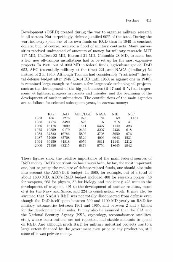
Postface 411
Development (OSRD) created during the war to organize military researchin all sectors. Not surprisingly, defense justified 90% of the total. During thewar, industry spent less of its own funds on R&D than in 1940 in constantdollars, but, of course, received a flood of military contracts. Many univer-sities received undreamed of amounts of money for military research: MIT117 MD, CalTech 83 MD, Harvard 31 MD, Columbia 28 MD, to name buta few; new off-campus installations had to be set up for the most expensiveprojects. In 1950, out of 1083 MD in federal funds, agriculture got 53, DoD652, AEC (essentially military at the time) 221, and NACA (similarly) 54instead of 2 in 1940. Although Truman had considerably “restricted” the to-tal defense budget after 1945 (13-14 BD until 1950, as against one in 1940),it remained large enough to finance a few large-scale technological projects,such as the development of the big jet bombers (B-47 and B-52) and super-sonic jet fighters, progress in rockets and missiles, and the beginning of thedevelopment of nuclear submarines. The contributions of the main agenciesare as follows for selected subsequent years, in current money:
Total DoD AEC/DoE NASA NIH NSF1953 1851 1275 278 84 59 0.1511958 4774 3480 828 97 218 411966 16178 7099 1441 5327 1142 3231975 19859 9179 2439 3207 2436 6181982 37822 16786 5896 3708 3950 9761987 57099 35708 5529 4096 6643 15311994 69450 34818 6959 8811 11141 22122000 77356 33215 6873 9754 18645 2942
These figures show the relative importance of the main federal sources ofR&D money. DoD’s contribution has always been, by far, the most importantone, but to gauge the real size of defense-related funds, one should also takeinto account the AEC/DoE budget. In 1968, for example, out of a total ofabout 1600 MD, AEC’s R&D budget included 400 for research proper (48for weapons, 265 for physics, 86 for biology and medicine); 425 went to thedevelopment of weapons, 491 to the development of nuclear reactors, muchof it for the Navy and Space, and 224 to construction work. It may also beassumed that NASA’s R&D was not totally disconnected from defense eventhough the DoD itself spent between 500 and 1100 MD yearly on R&D formilitary astronautics between 1961 and 1965, and between 2 and 3 billionfor the development of missiles. It may also be assumed that the CIA andthe National Security Agency (NSA, cryptology, reconnaissance satellites,etc.), whose contributions are not reported, had sizable amounts to spendon R&D. And although much R&D for military industrial projects was to alarge extent financed by the government even prior to any production, stillsome of it was private money.
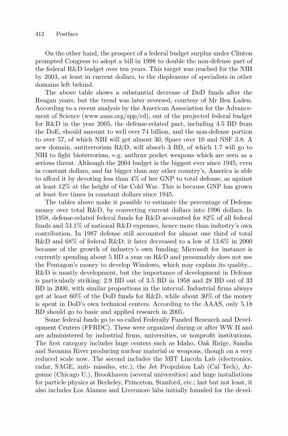
412 Postface
On the other hand, the prospect of a federal budget surplus under Clintonprompted Congress to adopt a bill in 1998 to double the non-defense part ofthe federal R&D budget over ten years. This target was reached for the NIHby 2003, at least in current dollars, to the displeasure of specialists in otherdomains left behind.
The above table shows a substantial decrease of DoD funds after theReagan years, but the trend was later reversed, courtesy of Mr Ben Laden.According to a recent analysis by the American Association for the Advance-ment of Science (www.aaas.org/spp/rd), out of the projected federal budgetfor R&D in the year 2005, the defense-related part, including 4.5 BD fromthe DoE, should amount to well over 74 billion, and the non-defense portionto over 57, of which NIH will get almost 30, Space over 10 and NSF 3.8. Anew domain, antiterrorism R&D, will absorb 3 BD, of which 1.7 will go toNIH to fight bioterrorism, e.g. anthrax pocket weapons which are seen as aserious threat. Although the 2004 budget is the biggest ever since 1945, evenin constant dollars, and far bigger than any other country’s, America is ableto afford it by devoting less than 4% of her GNP to total defense, as againstat least 12% at the height of the Cold War. This is because GNP has grownat least five times in constant dollars since 1945.
The tables above make it possible to estimate the percentage of Defensemoney over total R&D, by converting current dollars into 1996 dollars. In1958, defense-related federal funds for R&D accounted for 82% of all federalfunds and 53.1% of national R&D expenses, hence more than industry’s owncontribution. In 1987 defense still accounted for almost one third of totalR&D and 68% of federal R&D; it later decreased to a low of 13.6% in 2000because of the growth of industry’s own funding; Microsoft for instance iscurrently spending about 5 BD a year on R&D and presumably does not usethe Pentagon’s money to develop Windows, which may explain its quality...R&D is mostly development, but the importance of development in Defenseis particularly striking: 2.9 BD out of 3.5 BD in 1958 and 28 BD out of 33BD in 2000, with similar proportions in the interval. Industrial firms alwaysget at least 60% of the DoD funds for R&D, while about 30% of the moneyis spent in DoD’s own technical centers. According to the AAAS, only 5.18BD should go to basic and applied research in 2005.
Some federal funds go to so-called Federally Funded Research and Devel-opment Centers (FFRDC). These were organized during or after WW II andare administered by industrial firms, universities, or nonprofit institutions.The first category includes huge centers such as Idaho, Oak Ridge, Sandiaand Savanna River producing nuclear material or weapons, though on a veryreduced scale now. The second includes the MIT Lincoln Lab (electronics,radar, SAGE, anti- missiles, etc.), the Jet Propulsion Lab (Cal Tech), Ar-gonne (Chicago U.), Brookhaven (several universities) and huge installationsfor particle physics at Berkeley, Princeton, Stanford, etc.; last but not least, italso includes Los Alamos and Livermore labs initially founded for the devel-
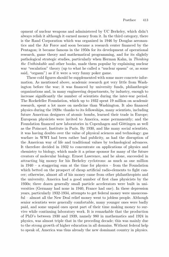
Postface 413
opment of nuclear weapons and administered by UC Berkeley, which didn’talways relish it although it earned money from it. In the third category, thereis the Rand Corporation which was organized in 1946 by Douglas aeronau-tics and the Air Force and soon became a research center financed by thePentagon; it became famous in the 1950s for its development of operationalresearch, game theory and mathematical programming, and for its slightlypathological strategic studies, particularly when Herman Kahn, in Thinkingthe Unthinkable and other books, made them popular by explaining nuclearwar “escalation” theory (up to what he called a “nuclear spasm” or, as somesaid, “orgasm”) as if it were a very funny poker game.
These cold figures should be supplemented with some more concrete infor-mation. As mentioned above, academic research got very little from Wash-ington before the war; it was financed by university funds, philanthropicorganizations and, in many engineering departments, by industry, enough toincrease significantly the number of scientists during the inter-war period.The Rockefeller Foundation, which up to 1932 spent 19 million on academicresearch, spent a lot more on medicine than Washington. It also financedphysics during the 1920s: thanks to its fellowships, many scientists, includingfuture American designers of atomic bombs, learned their trade in Europe;European physicists were invited to America, some permanently; and theFoundation financed new laboratories in Copenhagen and Gottingen as wellas the Poincare, Institute in Paris. By 1930, and like many social scientists,it was having doubts over the value of physical sciences and technology: gaswarfare in WWI had been rather bad publicity, as had the disruption ofthe American way of life and traditional values by technological advances.It therefore decided in 1932 to concentrate on applications of physics andchemistry to biology, which made it a prime sponsor for many of the futurecreators of molecular biology. Ernest Lawrence, and he alone, succeeded inattracting big money for his Berkeley cyclotrons: as much as one millionin 1940 – a staggering sum at the time for physics – from the Foundationwhich betted on the prospect of cheap artificial radio-elements to fight can-cer; otherwise, almost all of his money came from other philanthropists andthe university. America had a good number of first class physicists by the1930s; three dozen generally small particle accelerators were built in uni-versities (Germany had none in 1940, France had one). In these depressionyears, particularly 1932-1934, attempts to get federal money were unsuccess-ful – almost all the New Deal relief money went to jobless people. Althoughsenior scientists were generally comfortable, many younger ones were badlypaid, and some unpaid ones spent part of their time making money to sur-vive while continuing laboratory work. It is remarkable that the productionof PhD’s between 1930 and 1939, namely 980 in mathematics and 1924 inphysics, was almost triple that in the preceding decade; this was mainly dueto the strong growth of higher education in all domains. Without federal helpto speak of, America was thus already the new dominant country in physics.
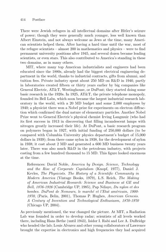
414 Postface
There were Jewish refugees in all intellectual domains after Hitler’s seizureof power; though they were generally much younger, less well known thanAlbert Einstein, and not always welcome as Jews at the time, many Ameri-can scientists helped them. After having a hard time until the war, most ofthe refugee scientists – almost 200 in mathematics and physics – were to findpermanent university positions after 1945, and several dozen became leadingscientists, or even stars. This also contributed to America’s standing in thesetwo domains, as in many others.
MIT, where many top American industrialists and engineers had beeneducated since the 1880s, already had the biggest electrical engineering de-partment in the world, thanks to industrial contracts, gifts from alumni, andtuition fees. Private industry spent about 250 MD on R&D in 1940, partlyin laboratories created fifteen or thirty years earlier by big companies likeGeneral Electric, AT&T, Westinghouse, or DuPont; they started doing somebasic research in the 1920s. In 1925, AT&T, the private telephone monopoly,founded its Bell Labs, which soon became the largest industrial research lab-oratory in the world, with a 20 MD budget and some 2,000 employees by1940; a physicist there won a Nobel prize for experiments on electron diffrac-tion which confirmed the dual nature of elementary particles. Another NobelPrize went to General Electric’s physical chemist Irving Langmuir (who hadits first success in 1913 in discovering that filling incandescent lamps withnitrogen greatly increased their life). At DuPont, a basic research programon polymers began in 1927, with initial funding of 250,000 dollars (to becompared with Columbia University physics department’s budget of 15,000dollars in 1939); from there came nylon in 1938, for the development of nylonin 1938; it cost about 2 MD and generated a 600 MD business twenty yearslater. There was also much R&D in the petroleum industry, with projectscosting from a few hundred thousand to 15 MD. This figure looked enormousat the time.
References: David Noble, America by Design. Science, Technologyand the Rise of Corporate Capitalism (Knopf, 1977), Daniel J.Kevles, The Physicists. The History of a Scientific Community inModern America (Vintage Books, 1979), L.S. Reich, The Makingof American Industrial Research: Science and Business at GE andBell, 1876-1926 (Cambridge UP, 1985), Pap Ndiaye, Du nylon et desbombes. DuPont de Nemours, le marche et l’Etat americain, 1900-1970, (Paris, Belin, 2001), Thomas P. Hughes, American Genesis.A Century of Invention and Technological Enthusiasm, 1870-1970(Chicago UP, 2004).
As previously mentioned, the war changed the picture. At MIT, a RadiationLab was founded in order to develop radar; scientists of all levels workedthere, including Hans Bethe (until 1943), Isidor I. Rabi and Lee A. DuBridgewho headed the lab; Louis Alvarez and other young collaborators of Lawrencebrought the expertise in electronics and high frequencies they had acquired
Postface 415
in Berkeley; many of these people became very influential science advisorsto the government after the war. At MIT and elsewhere, the work on radarrequired many advances in all domains of electronics, e.g. in high frequencies,or in semi-conductors because glass valves could not detect centimetric radarwaves. Methods for purifying germanium were found at Purdue and werecrucial to the invention of transistors a few years later, while Bell Labs didthe same, with less success, for silicon. The size of the radar business can begauged from the fact that the Rad Lab employed up to 4,000 people, whilethe industrial production proper cost almost 3 BD – more than the atomicbomb project.
Headed by General Groves, the Manhattan Project – that most spectac-ular success story, though less useful for winning the war – employed hun-dreds of scientists in Los Alamos and elsewhere; these included Fermi, Bethe,James Franck, Harold Urey, Arthur Compton, Lawrence, von Neumann, Al-varez, and even Niels Bohr, all of them (except von Neumann) past or futureNobel prizewin ners. Oppenheimer, a former Rockefeller fellow and the bestnative theoreti cian, headed Los Alamos with fantastic brio; he understoodeverything and made the whole enterprise succeed. He was under permanentsurveillance by the FBI who were well aware of his pre-war leftist leaningsand connections; this did not prevent the bombs’ blueprints from quietlyleaving Los Alamos for Moscow in a Plymouth driven by Klaus Fuchs in thesummer of 1945. The project cost two billion, 70% of which was spent on theproduction elsewhere of U-235 in a gigantic isotopic separation factory or inLawrence’s calutrons, and of Pu in huge atomic piles. Most of the basic tech-niques later used in civilian nuclear energy were invented between 1942 and1945, and this allowed General Electric, Westinghouse, DuPont and othercompanies to learn them and to become world leaders after the war in usingnuclear power for electricity production, and first of all for the propulsion ofsubmarines or aircraft carriers. More about this in the Internet file.
In 1945-1946, nuclear physicists were rewarded with millions left over fromthe Manhattan Project, which allowed them, among other consequences, tobuild new particle accelerators whose cost eventually came to billions (notmillions). Before 1940, this prospect would have been dismissed as utterlyinsane. The AEC/DoE has funded this domain in America from 1947 to thisday, while the Rockefeller Foundation withdrew its support after 1945 sincethe government could provide far more; in addition, since 1941 Lawrenceand others had been hinting at spreading radioactive waste over or in frontof enemy troops in case of war, which was not quite as glamorous as fightingcancer.
In a famous 1945 report, Science, the Endless Frontier , the chief of mili-tary R&D (OSRD) during the war, Vannevar Bush, advocated the establish-ment of a National Science Foundation funded by the government and whosepresident and programs would be chosen by scientists; the project was re-jected by the President. It came into being in 1950 as a federal agency funded
416 Postface
and governed by the government and controlled by Congress like other agen-cies, with, of course, plenty of scientific advisory committees; but it got verylittle money before Sputnik, as the table above shows. In the bio-medicalsector, where a first National Cancer Institute had been founded in 1937,new National Institutes of Health were established; with strong backing fromCongress and voters, they continued to grow and multiply and are now byfar the most important non- defense source of federal money. Meanwhile, theOffice of Naval Research founded in 1946 spent some 20 MD per year to helpresearch in all domains, mainly to keep in touch -“in case” – with scientistsand research; mathematics got about 10%, but a threateningly increasingpart of it (up to 80% in 1950) was – already! – funding the development atMIT of a futuristic Whirlwind computer working in real time; a riot ensued,and Whirlwind would have died but for the birth of a far better sponsor in1950, namely the air-defense system of the American continent, as we shallsee later.
Private universities, where government interference was anathema before1940, reversed their principles: ONR was very liberal and people got used tothis new kind of “tainted money”; after all, nobody had ever asked trustees orbenefactors of the rich universities how they became so wealthy; but it some-times took several years before federal money (and possibly classified militarycontracts) were accepted. CalTech was still a small university in 1945; witha board of trustees made up of very conservative bankers and industrialistswho approved the policy of basic research presided over by physicist and No-bel Prize winner Robert Millikan, it was several years before it bowed to theinevitable; meanwhile, the off-campus Jet Propulsion Laboratory founded byvon Karman prospered on guided missiles and DoD money, as was the caseat Johns Hopkins with the Applied Physics Laboratory founded during thewar. Julius Stratton, a future president of MIT who during the war had closeties with the higher echelons of the Pentagon – he was one of the stars of theMIT Radiation Lab -, wrote in October 1944 to MIT president:
Twenty-five years ago everyone talked about the end of war; todaywe talk about World War III, and the Navy and Air Force, at least,are making serious plans to prepare for it. Inevitably this nationalspirit will react upon the policies of our educational and researchinstitutions. It always has, and we might just as well face it (...)We shall have to deal with the Army and Navy and make certainconcessions in order to meet their needs.
This means that by 1950, 85% of the MIT total research budget came fromthe military and AEC, with a still higher proportion for physical sciences inother elite universities. John Terman, another star in electronics, wrote in1947 to his university’s president that
Postface 417
Government-sponsored research presents Stanford, and our Schoolof Engineering, with a wonderful opportunity if we are prepared toexploit it,
which of course they were. The importance to the military of these univer-sity departments was due not only to their research work, but also to theireducating thousands of scientists and engineers for defense work in particular.
References: Everett Mendelsohn, Merritt Roe Smith and Peter Wein-gart, eds., Science, Technology and the Military (Kluwer, 1988), PaulForman & J.M. Sanchez- Ron, eds, National Establishments andthe Advancement of Science and Technology (Kluwer, 1996), Stu-art W. Leslie, The Cold War and American Science: The Military-Industrial-Academic Complex at MIT and Stanford (Columbia UP,1993).
Various more or less successful attempts were made after 1950 to bring sci-entific advice to the highest levels of government, particularly the DoD; itwas Sputnik which brought scientists to the White House. Meanwhile, theKorean War was an opportunity to organize “summer studies” during whichscientists, engineers and military men would gather for several weeks in or-der to study such (classified, i.e. secret) defense problems as anti-submarinewarfare, tactical nuclear weapons, air defense, etc.
The size of American defense activities in the 1950s and 1960s can easilybe explained by political factors and by reactions to perceived Soviet threats(or counter-threats to perceived American threats: bombs, bombers to deliverthem, and the “encirclement” of the USSR by US air bases). As we have seen,the first Soviet atomic test launched America into the race for the H-bomb.In the spring of 1950, the celebrated NSC-68 report of the White HouseNational Security Council, vastly exaggerating the Soviet military threat andsupposed plans for world domination, recommended (among other things, e.g.much stronger West European forces) a huge increase of the Defense budget;the figures which were known but remained unwritten, namely 40- 50 billioninstead of 13-14, were judged excessive even by the military, who did notknow how to spend so much money. Truman did not agree either, but the“Socialist camp” forced it on by sparking the Korean War. In particular, theproduction capacity for U-235 and Pu was increased in a staggering way: fivenew piles for the production of Pu, one for the production of tritium, and twomore huge isotopic separation units, with sixteen times the capacity of the1945 factory, which had already been enlarged; up to 85 tons of U-235 couldbe produced per year, which needed 6,000 megawatts of electricity, or 12% oftotal US production. Nuclear weapons of all types grew in America at a rateof several thousand per year, to reach 32,000 in 1964, with powers rangingfrom a few tens of tons up to several megatons in TNT equivalence. Thiswas about fifteen times the Soviet arsenal at the time and could be deliveredby 800 intercontinental ballistic missiles (ICBM), 200 submarine-launched
418 Postface
missiles (SLBM), a thousand fighter- bombers based in Europe, the MiddleEast, Japan or on aircraft carriers, and strategic bombers (about 2,000 B-47and 700 B-52 were built before 1962).
A gigantic system to defend America against Soviet bombers was built,as we are now going to see. The first Soviet atomic bomb led people at MITto take the first steps to protect the USA from future Soviet bombers in 1950(this threat was dismissed by Curtis LeMay, the Strategic Air Command(SAC) chief during the 1950s: his personal strategy was to wipe out Sovietplanes, copies of the US B-29 bombers of 1944 vintage, before they could takeoff, but bypassing the President was slightly illegal...). This originally smallProject Lincoln based on the Whirlwind computer led to the founding of aLincoln Lab at MIT, and to the gigantic SAGE system of continental defense– a precursor to SDI -, at a cost of 30 billion (or 200 billion in 1996 money,and much more if personnel and other costs are included). Thousands of BellLabs Nike-Hercules missiles, each carrying a 2 to 30 KT atomic warhead,could destroy entire fleets of incoming aircraft , assuming the Soviets wereclever enough and able to send such fleets over the North Pole in suicideraids since, in any case, they could not make the round trip until big jets –never more than 200 – began to appear in 1955. Bell Labs, which had de-veloped anti-aircraft rockets since 1945, managed everything while hundredsof subcontractors in practically all domains of technology helped develop thehardware and software needed in SAGE. SAGE was obsolete as soon as itbecame operational in 1960- 1962: bombers were replaced by unstoppablemissiles after 1962, which led to the first and useless anti-missile systems,including the highly controversial Nike-Zeus missiles with 60 to 400 KT war-heads, based around big cities and never deployed. The USSR’s programevolved in similar fashion, but was even more expensive since missiles andbombers could come from many directions.
The SAGE project however played a major role in all kinds of tech-nical advances, particularly long-range “over- the-horizon” radars, guidedanti-aircraft weapons, and computers. In this last field, it led to magneticcore memories, video displays, light pens, graphics, simulation, synchronousparallel logic, analog-to-digital conversion and transmission of radar dataover telephone lines via the first transistorized modems made by Bell, multi-processing, automatic data exchange between different computers, etc. Withits hundreds of thousand lines of code and hundreds of computer screens,SAGE provided the first opportunity to train several thousand programmers(most of whom later went to industry); this was done by the SDC branchof the Rand Corporation, which was founded in 1957 to that effect. Amongmany other machines, SAGE needed fifty six IBM AN/FSQ-7 and -8 (or“Whirlwind II”) computers; there were twenty-four SAGE main commandcenters connected to a pharaonic installation under the Colorado mountains,itself connected to the White House and Pentagon; each of the centers usedtwo of these IBM computers working in tandem to increase reliability. Made
Postface 419
to order at a cost, in current money, of 30 million a piece, each of thesemachines weighed 275 tons, had some 60,000 valves, used 32-bit words, hada magnetic core memory – one of the great innovations from Whirlwind –of about 270 kilobits, twelve magnetic drums each storing 12,288 words ofprogram, and was connected to about one hundred screens displaying enemyplanes’ trajectories and enabling operators to vector fighter planes graphi-cally. It needed 750 kw of electric power to run and a hurricane to evacuatethe heat it generated. These performances may look puny by 2005, but therewas nothing more powerful at the time and, of course, the new techniqueswere put to good use in IBM’s future commercial computers. All of the lat-ter were transistorized after 1960, the first large ones (series 7090) beingdelivered to the three gigantic radars of the Ballistic Missiles Early WarningSystem in Alaska, Greenland and Scotland.
References on SAGE: chap. 4 of Atomic Audit , Edwards’ chap. 3,Kent C. Redmond and Thomas M. Smith, From Whirlwind to Mitre.The R&D Story of the SAGE Air Defense Computer (MIT Press,2000), very weak on technology, and Thomas P. Hughes, RescuingPrometheus (Random House, 1998).
Then came Sputnik in October 1957, which scientists used very success-fully to clamor for increased research funds. NACA was transformed intoNASA, with very soon a budget in billions of dollars, while the Defense bud-get proper decreased. A scientific committee (PSAC) was instituted at theWhite House. The Advanced Research Projects Agency, ARPA, was foundedby the DoD in order to fund and organize the most sophisticated researchprojects with military implications. Americans reacted to the “missile gap”with wild and shifting predictions on the size of the Soviet arsenal (100 in1959, 500 by 1960 and 1,000 by 1961-1962) from the CIA, the Air Force, jour-nalists, and democrat politicians, including Kennedy and especially Johnson,wishing to destroy the 1952-1960 Eisenhower republican administration. Butradars from Turkey and Iran had detected Soviet missile tests in 1953-1954,and, from 1955 on, absolute priority was given to similar American programs,Atlas and Titan, soon followed by the silo protected Minuteman series ofICBMs, the Polaris missiles for nuclear submarines, and the first satellitesfor reconnaissance, infrared detection of missile firings, meteorology, commu-nications, etc (1959-1961). Extended flights over Soviet territory first by U-2spy planes, then satellites, proved in 1960 that there was indeed a big “missilegap”: perhaps four Soviet operational missiles, to dozens of American ones.
Like the Korean War, Sputnik and Khrushchev’s boasts proved to be aself-defeating move and another wonderful opportunity for the American andSoviet “scientific-military- industrial complexes”. The Soviet arsenal, vastlyoutnumbered by the American arsenal until the 1970s, was nevertheless bigenough to make an American attack unlikely, and in any case America’stop political rulers found the Air Force’s apocalyptic war plans quite repel-lent, although they knew they might have to “push the button” as a last
420 Postface
resort (see my vol. I, p. 122; in 1960, over 150 weapons were reserved forthe Moscow area alone, and quite a number of them would have destroyedeach other). To paraphrase a journalist writing in Science , September 27,1974, these huge defense systems were the cathedrals of a century that futurehistorians will characterize by its extraordinary technical capacities and itspermanent devotion to the mortuary arts. And so on, with ups and downs,until the fall of the Soviet Union. The most exotic parts of Reagan’s StarWars project were terminated, but a less ambitious anti-missile program isstill going on, at the rate of several BD per year, with a first deployment inAlaska of weapons guided on a collision course with enemy missiles (a fasci-nating problem in Control Theory) although no one can guess who would befoolish enough to launch them. America’s military doctrine is now undergo-ing a “Revolution in Military Affairs” based on “Space Dominance”, whichaims at fully integrating every weapon and everyone – from the President andthe Pentagon warlords down to the GI on the battlefield – through all kindsof satellites, drones, telecommunications, information networks, etc. You willfind an impressive survey of it in Introduction au siecle des menaces (Paris,Odile Jacob, 2004), by Jacques Blamont, a French specialist in Space Scienceswith long and strong ties to the Jet Propulsion Lab (and, more recently, So-viet astronautics), and a member of the US Academy of Sciences. Another“revolution” has been under way since the Strategic Computing Initiativeof the 1980s: substituting all kinds of “intelligent” robots for weak mortalson the battlefields of 2030, according to the New York Times (02/16/2005).Contracts worth 127 BD have already been issued for this Future CombatSystems project, which will contribute to boosting weapons acquisition costsfrom 78 BD now to 118 by 2010. Those who believed the end of the Cold Warwould slow down the technical progress of armaments were badly mistaken...
The development of nuclear weapons, fighter planes, bombers, missiles,nuclear submarines, aircraft carriers, SAGE, satellites for C4 RI (command,control of operations, communications, computers, reconnaissance and intel-ligence), etc. relied on and greatly encouraged technical progress in dozens ofless spectacular domains: electronic components (from glass valves to tran-sistors to printed circuits to integrated circuits to VLSI...), computer hard-ware and software, navigation and guidance systems, infrared detection, firecontrol devices, radar and sonar, microwave propagation, space telecommu-nications, materials, etc. The list is endless.
The development of transistors and integrated circuits is a good example.Semi-conductors had been known for a long time and were the first detectorsused in wireless in the 1900s. Systematic experimental studies in the 1930sand during WW II, as well as the development of a solid-state theory usingquantum mechanics, had led to a good understanding of the phenomena by1945, and, at Purdue university, to methods of obtaining highly purified ger-manium (so named by its German discoverer), from which rectifying diodeswere mass produced for radar detection. The Bell Labs did the same with sili-
Postface 421
con with less success at the time. After 1945, they tried to discover solid-stateamplifiers, and the first very primitive point-contact transistors were madethere in 1947 by two physicists, John Bardeen and Walter Brattain, headedby William Shockley who a few years later found a way to make industrializa-tion far easier; all three shared a Nobel Prize. Transistors, patented by Bellin 1948, were expected to replace electronic valves and electro-mechanicalswitches in a myriad of devices used by the AT&T telephone system. Butthere was nothing urgent here – the capital invested in standard equipmentwas far too high to be scrapped – and, anyway, replacement would requireyears of further development and industrialization. AT&T, however, was un-der an anti-trust suit at the time and the military watched the developmentof transistors with great interest. Bell therefore organized a first informa-tion meeting at the beginning of 1951 for military and government officialsonly, then a symposium in September for some three hundred American andEuropean engineers to whom the characteristics of a dozen transistors weredisclosed. In 1952, Bell decided to sell its patents to 36 companies and, inApril, to divulge the know-how to licensed companies. A first productionunit for military transistors was built by Western Electric, the manufactur-ing branch of AT&T. The anti-trust suit ended in 1956 and, among otherclauses, AT&T was ordered to limit its production to its own needs and tothe government market, for which many Bell innovations were made; thisfavored other manufacturers. The Army Signal Corps had already issuedproduction contracts to twelve makers for use in the forthcoming strategicmissiles, and demanded 3,000 units of thirty different types per month. Sinceat that time only 5 to 15% of the production was free of defects, this re-quired much higher production capacities, with very high unit costs. But therate of rejects, and hence prices, soon dropped, and sales to less demandingbuyers went from 14 million in 1956 to 28 million in 1958. The military wereinterested in transistors because they were small and light, consumed verylittle power, and were much less sensitive to shocks, vibrations and wear thanvalves. First models of transistorized computers were built at Bell Labs andLincoln Lab (MIT) in the 1950s, for the military, of course.
The first civilian commercial uses of transistors were for hearing aids(Raytheon, 1954) costing 150-200 dollars; transistor portable radios came afew years later. It took at least ten years before a large commercial marketdeveloped because classical valves were far cheaper – one dollar instead ofeight around 1953 -, had much better characteristics than early transistors,were much easier to make, and were much more familiar to most electronicsengineers; the main advantages of transistors were not needed in most ap-plications, though they attracted the military. Between 1954 and 1956, themarkets for transistors and valves were $55 and over 1000 million respectively.And though several established valve manufacturers (General Electric, RCA,etc.) had 31% of the market in 1957, new and much smaller firms (Texas
422 Postface
Instruments, formerly a geophysical services company, Transistron, Hughes,etc.) had 64%.
Integrated circuits were invented in 1958 by Texas Instruments withoutmilitary funding (military projects for miniaturizing electronic circuits allfailed or came too late in the 1950s), but their mass production was madepossible by the invention of the so-called planar process for silicon transistorsby a group of eight physicists and engineers who left a company the insuf-ferable Shockley had founded in 1954. The Fairchild Company which, sincethe 1920s, made aerial cameras and later components of analog computers(all mostly for the military), set up for them the Fairchild SemiconductorCorporation in 1957. Since they had their eye on the commercial market –some of them founded Intel a few years later -, they rejected military R&Dcontracts to remain free of having to develop products which, although mil-itarily important, would be of little commercial interest. They neverthelessdecided to concentrate first on the improvement and manufacture of highperformance silicon transistors for the military market. This was the timethe military was beginning to replace analog computers with digital ones inavionics and missiles because only silicon – and neither very expensive ger-manium, nor electronic valves – could stand the high temperatures, shocksand vibrations prevalent in many military systems. Their first customer wasIBM which bought one hundred Fairchild “mesa” transistors at 150 dollars apiece for use in the navigational computer for the prototype of the B-70 su-personic bomber they had already made the analog computers for the B-52s,a much bigger market). They had no competitor other than Bell Labs, theirmesa transistors immediately found many other avionics uses, and their salesjumped from 65,000 dollars in September 1958 to 2.8 MD for the first eightmonths of 1959. Their most important customer was Autonetics, in charge ofdeveloping the digital computer guidance system for the Minuteman missile.Other early uses included an air-to-air missile, a torpedo, and the Apollospace station. Problems of reliability led to the “planar process” to makemuch better transistors; the rate of defect-free components was 5% at first,but they were under such pressure from Autonetics, which demanded oneyear without failure, not to mention the now growing competition in mesatransistors, that they persisted, then developed ultra-reliable planar diodesfor computers and eventually integrated circuits. The planar process madeit possible to fabricate many components on the same silicon wafer and toconnect them, again with a very low initial proportion of defect-free circuits.All of this looks very simple, but required extraordinary standards of clean-liness, manufacturing skills, and an unprecedented level of discipline on theworkforce , as one of my sources said.
Total sales of ICs amounted to 4 MD in 1962, 41 in 1964, 148 in 1966and 312 in 1968, while the average unit price dropped from 50 dollars to2.33; in those same years the military bought 100%, 85%, 53% and 37% ofthe total sales. More generally, the military part of the electronics industry’s
Postface 423
total sales, which was 24% in 1950, climbed to 53-60% during the years1952-1968. The general pattern in electronics at the time was that the firstcustomers, namely the military and their industrial contractors, bought theinitial product at prices which included most of the R&D and at least partof the tooling; prices then went down to a level which civilian industry andbusiness could afford for their own uses, which in time lowered the pricesagain until the general public could buy solid-state gadgets like radios, TVsets or PCs. With a huge civilian market after 1980, chip makers like Intelcould continue to improve their products with little help from the military;Intel even refused to work on highly sophisticated very high speed circuits(VHSIC) with no civilian uses.
The military actually benefited from this civilian market as they tooneeded a lot of standard electronics that could be purchased off-the-shelf atlow prices. For this reason and to help American industry against Japanesecompetition, they became interested in “dual” technologies with military andcivilian uses. The DoD still spends about 25% of its R&D budget on electron-ics and communications, but for more sophisticated products than personalcomputers...
The early development of computers was still more influenced by the mil-itary. Explaining it here would take too much space; see the Internet file. I’llmerely point out that the 35 computers made between 1945 and 1955 wereentirely financed by the DoD, with the exception of two in universities whichmy source does not know, and of the von Neumann Princeton computerwhich was financed by the Army, Navy, AEC and RCA (but its five copieswere financed by AEC or, at Rand, by the Air Force). Almost all of thesemachines were one of a kind; only three companies made several productionunits: UNIVAC, the company Eckert-Mauchly had founded in 1947 in orderto make huge data-processing machines with the commercial market (bank-ing, insurance, etc.) in mind, although it also had military customers; ERA,founded by a team of former cryptologists from the Navy who made veryadvanced computers for the National Security Agency; and IBM which, atthe start of the Korean War, decided to make digital machines. They lookedfor customers and found seventeen, either military or in the military indus-try. Of course a huge civilian market developed later – mainly after 1960 -,but the influence of military research contracts and procurement always wasextremely powerful, and still is.,
References: Herman H. Goldstine, The Computer: From Pascal tovon Neumann (Princeton UP, 1972), Kenneth Flamm, Targetingthe Computer (1987, Brookings Inst. Press) and Creating the Com-puter: Government, Industry, and High Technology (1988, Brook-ings), Arthur L. Norberg and Judy E. O’Neill, Transforming Com-puter Technology. Information Processing for the Pentagon, 1962-1986 (1996, Johns Hopkins UP), Donald MacKenzie, Knowing Ma-chines (MIT Press, 1998), Janet Abbate, Inventing the Internet
424 Postface
(1999, MIT Press). National Academy of Sciences, Funding a Rev-olution. Government Support for Computing Research (NAS Press,1999), very explicit and thankful to the DoD, Alex Rolland & PhilipShiman,Strategic Computing: DARPA and the Quest for MachineIntelligence (MIT Press, 2002).
Below industry level, all domains of science, from mathematics and computerscience to nuclear physics, electronics, optronics,..., oceanography, geology(used e.g. for monitoring underground nuclear tests) and even to some extentbiology and medicine, expanded tremendously since much of their results andmany experts were needed in all domains of high technology and defense.
§ 3. Applied mathematics in America
In the entertaining chapter of his autobiography, Un mathematicien auxprises avec le siecle (Paris, Odile Jacob, 1997, trad. Birkhaser), which hedevotes to his teaching at the Ecole polytechnique, Laurent Schwartz ac-cuses (p. 355) the French pure mathematicians , and especially the Bourbakigroup, of having ostracized their applied colleagues. As a matter of fact, forat least ten years there was nearly nobody to be “ostracized” before the riseof Jacques-Louis Lions (1928-2001), a very bright student of Schwartz whofirst worked on distributions and partial differential equations (PDEs) in themodern way made possible by the development of functional analysis. Hediscovered applied mathematics and computers in America in 1956 in cir-cumstances that will be explained below, and later founded the very brilliantFrench School of Applied Mathematics; he himself was appointed a professorat Nancy in 1954, in Paris in 1963, at the Polytechnique (1965-1986), and atthe College de France in 1973.
From 1980 to 1984, he headed the French government National Insti-tute for Research in Informatics and Automatics (INRIA) with which he hadbeen connected for ten years, the French NASA (CNES) from 1984 to 1992,and he won some of the highest international prizes; quite a victim of our os-tracism, and otherwise a great mathematician with some 50 doctoral studentsand hundreds of “descendants” in the world. See a substantial biography byRoger Temam, one of his principal students, at www.siam.org/siamnews/07-01/lions.htm.
Schwartz decrees that every mathematician must concern himself with theapplications of what he is doing without, it seems, being aware of the factthat “to concern oneself with” may have quite a number of different mean-ings, whether in French or in English. He provides neither a justification forhis categorical imperative nor the slightest account of the very diverse appli-cations of mathematics. The fact that applied mathematics were undergoinga powerful expansion in the United States and USSR among others seems to
Postface 425
justify everything, without it being necessary to explain this strange and verynew development in the two countries which led the arms race until 1990.
The development of applied mathematics in the USA which so inspiredSchwartz is not too difficult to explain, even though much remains to bedone since physics and technology, being far more spectacular, have almostmonopolized historians until now. The Soviet situation, although less wellknown, was certainly no better.
Before the war, “pure” mathematics prevailed in universities everywhere(except in the USSR, since this “bourgeois” concept was anathema to Marx-ism); engineers and physicists almost always solved their mathematical prob-lems by themselves, even when the new quantum mechanics obliged physicistseverywhere to rediscover strange mathematics. By the 1930s, the situationbegan to change in a few places, partly due to the arrival of European Jew-ish refugees. Richard Courant, Kurt Friedrichs, Fritz John and Hans Lewybrought to New York university some of the Gottingen tradition founded byFelix Klein forty years before. They dealt less with applied mathematics aswe know them – computers had yet to come – than with often “modern”mathematics such as found in Courant and Hilbert’s celebrated Methodender Mathematischen Physik . In 1937, the Army Ballistic Research Labora-tory at Aberdeen set up a scientific committee including von Neumann andvon Krmn besides other luminaries. Von Karman, formerly a student andlater a competitor of Ludwig Prandtl, the foremost German aerodynamicistin Gottingen, had been at CalTech since 1934 (and part-time since 1926),where he founded the future Jet Propulsion Laboratory. In 1945 he becamethe Air Force’s main scientific advisor and, in this capacity, one of the firstpromoters of atomic missiles. Classical Calculus being often sufficient, theWW II military R&D organization did not at first enlist mathematicians.Mainly at the request of mathematicians themselves, an Applied Mathemat-ics Panel was set up in 1942 with teams in several universities put at every-one’s disposal; they were, so to speak, the coalers of the R&D Dreadnoughtsof which the officers were physicists. Stanislas Ulam, who later became chiefmathematician at Los Alamos, had to ask his friend von Neumann for hishelp in getting war work in 1943. Applied (or, as Saunders McLane said,applicable) mathematics, much of it boring, blossomed in all kinds of fields,and some people converted to it for life. Shock waves propagation, surfacewaves in water of variable depth, “hydrodynamics computations” for theNagasaki bomb, gas dynamics, statistical optimization of air bombings andanti-aircraft defense, operational research, statistical quality control for themass production of weapons, etc. For anti-aircraft defense, Norbert Wienerinvented statistical prediction methods based on harmonic analysis and ana-lytical functions, but they were too sophisticated: he had been lured into themathematics of the problem. Transmitting orders or conversations in a secureway, that is to say unintelligible to non-authorized people, was very difficult,particularly communications between such high level persons as Roosevelt,
426 Postface
Churchill or Eisenhower. This was intensively studied at Bell Labs, wheredigitalization of continuous speech was apparently invented, while separatefrequency bands were encoded by adding random numbers and reductionmodulo 6 (it took quite a while for Bell’s engineers to discover it, althoughthey were familiar with mod 2 arithmetic); each encoding system was usedonly once, and recorded on two highly precise phonograph records, one ofwhich was used at the sending end and the other sent in advance to thereceiving end; this involved a lot of very complex electronics using kilowattsof power to transmit milliwatts of speech, and the help of some people withmathematical abilities which the electronics engineers lacked. One of themwas Claude Shannon, until 1941 at MIT and Princeton where he had studiedapplications of “Boolean algebra”, i.e. set theory, to the analysis of electroniccircuits; he derived from his work at Bell Labs the Information Theory thatmade him famous after the war. If you understand electrical engineering,see A History of Engineering and Science in the Bell System. National Ser-vice in War and Peace (1925-1975) (Bell Telephone Laboratories, 1978), pp.291-316.
Most postwar standard mathematical publications, written by mathe-maticians who are too busy or too discreet to consult sources, contain onlyrather abstract and summary generalities about the relevant mathematics.But luck may help those who read books that mathematicians generally donot open, or know of, since they don’t deal with mathematics.
The 1945 bombings on Japanese cities (and earlier ones on Germany)led to a fascinating problem: to determine the right proportion of explosiveand incendiary bombs for maximum damage. A Berkeley statistician, JerzyNeymann, was then called to help; he used methods which, after the war,made him a celebrity. Mathematical details are not to be found in my source,and it is likely that Neymann’s contribution was less useful than those ofscientists, led by Harvard chemist Louis Fieser, who in 1942 invented napalm,among other incendiaries, though it was not widely used until the war inKorea. During a bombing raid, planes were supposed to drop bomb clustersat 50-foot intervals, which would open at 2,000 feet and disperse 38 smallerbombs, starting a dozen fires; thus a B-29 was able to set fire to a 350x2,000-foot area. Relying on statistical computations to get the best results wouldthus have been a good idea (or a bad one, depending on your point of view).But recent books suggest that the method was discovered experimentally.
On the other hand, the task of choosing targets, based at first on theircontributions to Japanese armaments, and of evaluating the weight of bombsneeded, was conferred on a Committee of Operations Analysts which reliedon methods developed in Britain, mostly by physicists like P.M.S. Black-ett, initially for anti-submarine warfare, then for bombing operations. Theseproblems involved fairly simple mathematics but gave rise soon after the war(first of all at the Rand Corporation) to an extravagant amount of hypein favor of game theory, Operations Research, and linear or dynamic pro-
Postface 427
gramming; it was claimed they were the truly “modern” mathematics thatcould be applied to “solve the problems of society” – logistics, bombers bas-ing, optimizing a massive nuclear strike in case of war, dispatching packs ofCoca-Cola to troops in the field or grocery stores, etc. No wonder these dis-ciplines, which were still rather primitive mathematics assisted by the firstcomputers, did not attract everyone after the war even if they found harmlessapplications later:
What are we to think of a civilization which has not been able totalk about killing almost everybody, except in prudential and game-theoretical terms,
a good question Oppenheimer asked on TV in February 1950 or perhaps in1959 – my sources do not agree.
In the atomic sector, where the most difficult problems were to be found,the development of the implosion bomb (Nagasaki, plutonium) forced theo-reticians, headed by Hans Bethe, to solve numerically the PDEs governingthe propagation of the convergent shock wave produced by classical explo-sives surrounding a sub-critical ball of plutonium. At hundreds of thousandsof bars of pressure, plutonium behaves like a viscous fluid which you have tokeep perfectly spherical, whence a “hydrodynamics” problem as they calledit. To get the needed spherical shock wave required an assembly of 32 pentag-onal pyramids of fast explosives, with a half-sphere (“lens”) of slow explosivesin the middle of each one. Ready in the Spring of 1945 after thousands oftests, this device required solving countless problems by American and Britishexperts in explosives, many of them academics. Von Neumann contributedsignificantly to this effort in recommending that much larger amounts ofconventional explosives be used than was projected, as well as in the designof the explosive lenses; after having learned chemical engineering at ZurichPolytechnicum in his youth, he had participated at Aberdeen in the devel-opment of “shaped charges” for anti-tank projectiles. Hans Bethe, a nuclearphysicist who knew a lot of mathematics, wrote a 500- page report on shockwaves at Los Alamos.
To solve the two-dimensional PDE (three-dimensional computations werebeyond them until the 1980s), they first used the same classical finite dif-ference method as for one-dimensional problems. It turned out that smallvariations in the dimensions of time and space steps led to large variationsin the results: instability. Richard Courant was then called to the rescue. Heexplained to Bethe the successive approximations method that Friedrichs,Lewy and himself had used (Math. Annalen, 1928) to prove the existence ofsolutions: it prescribes non-obvious restrictions on the relative dimensions ofthe time and space steps used. It is at Los Alamos, it seems, that the firstopportunities to use the method arose. Thanks to that,
428 Postface
very soon problems involving fluid dynamics, neutron diffusion andtransport, radiation flow, thermonuclear reactions and the like werebeing solved on various machines all over the United States
writes Bethe’s first successor as chief of theoretical physics at Los Alamos, D.Richtmyer, in a 1957 book explaining, among other things, advances madeafter the war by von Neumann and Peter Lax concerning the convergence andstability of approximations; Banach spaces could now be used indirectly tounderstand what went on inside a bomb, for obviously this is what everybodywas interested in at the time in Los Alamos. Lax, who spent his summers atLos Alamos during the 1950s, was one of applied mathematics’ rising starsand, later, a strong opponent of Bourbaki’s mathematics. He once wrote ofVietnam war opponents who wanted to enlist the AMS that most of themspecialize in branches of mathematics that are abstract, often esoteric, andcompletely unmotivated by problems of the real world , thus implying that, hadthey instead busied themselves with, say, the mathematics of shock waves,they would have had no qualms over B-52s flattening Laos...
J-L. Lions, mentioned above, said much later in an interview (Le Monde,May 8, 1991) that he discovered applied mathematics and computers inAmerica in 1956 thanks to Lax, who told him of von Neumann’s ideas; aftermentioning a few current civilian applications, Lions treats us to an eulogyof von Neumann,
the father of the discipline who, at the end of the 1940s, was soable to guess all the benefits that would result from the use of thefirst computers to describe such complex systems as meteorologicalphenomena,
and that he himself only added one chapter which von Neumann had notentered: the industrial chapter (with enough success to be a member of theboard of several big French industrial companies during his last years). VonNeumann’s (and the Air Force’s) interest in meteorology is well known but,as the reader already knows, he was interested in other uses of computers.By 1956,
[his] combination of scientific ability and practicality gave him a cred-ibility with military officers, engineers, industrialists, and scientiststhat no one else could match. He was the clearly dominant figure innuclear missilery.
This other eulogy is from Herbert York Race to Oblivion (Simon & Schus-ter, 1970, p. 85); the was a member of the Teapot Committee which, chairedby von Neumann, chose in 1954-1955 the characteristics of ATLAS, the firstintercontinental missile. Lions may not have been told in 1956 of von Neu-mann’s taste for military projects, but in 1960, the year he started a seminaron numerical analysis in Paris, his first “really applied” paper was on nu-clear reactors. That he did not even hint in a 1991 interview at the huge
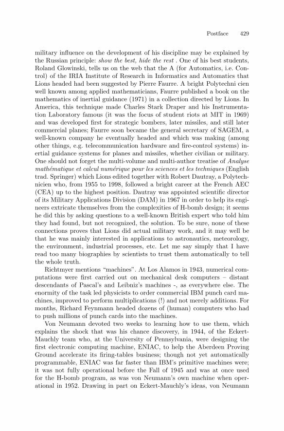
Postface 429
military influence on the development of his discipline may be explained bythe Russian principle: show the best, hide the rest . One of his best students,Roland Glowinski, tells us on the web that the A (for Automatics, i.e. Con-trol) of the IRIA Institute of Research in Informatics and Automatics thatLions headed had been suggested by Pierre Faurre. A bright Polytechni cienwell known among applied mathematicians, Faurre published a book on themathematics of inertial guidance (1971) in a collection directed by Lions. InAmerica, this technique made Charles Stark Draper and his Instrumenta-tion Laboratory famous (it was the focus of student riots at MIT in 1969)and was developed first for strategic bombers, later missiles, and still latercommercial planes; Faurre soon became the general secretary of SAGEM, awell-known company he eventually headed and which was making (amongother things, e.g. telecommunication hardware and fire-control systems) in-ertial guidance systems for planes and missiles, whether civilian or military.One should not forget the multi-volume and multi-author treatise of Analysemathematique et calcul numerique pour les sciences et les techniques (Englishtrad. Springer) which Lions edited together with Robert Dautray, a Polytech-nicien who, from 1955 to 1998, followed a bright career at the French AEC(CEA) up to the highest position. Dautray was appointed scientific directorof its Military Applications Division (DAM) in 1967 in order to help its engi-neers extricate themselves from the complexities of H-bomb design; it seemshe did this by asking questions to a well-known British expert who told himthey had found, but not recognized, the solution. To be sure, none of theseconnections proves that Lions did actual military work, and it may well bethat he was mainly interested in applications to astronautics, meteorology,the environment, industrial processes, etc. Let me say simply that I haveread too many biographies by scientists to trust them automatically to tellthe whole truth.
Richtmyer mentions “machines”. At Los Alamos in 1943, numerical com-putations were first carried out on mechanical desk computers – distantdescendants of Pascal’s and Leibniz’s machines -, as everywhere else. Theenormity of the task led physicists to order commercial IBM punch card ma-chines, improved to perform multiplications (!) and not merely additions. Formonths, Richard Feynmann headed dozens of (human) computers who hadto push millions of punch cards into the machines.
Von Neumann devoted two weeks to learning how to use them, whichexplains the shock that was his chance discovery, in 1944, of the Eckert-Mauchly team who, at the University of Pennsylvania, were designing thefirst electronic computing machine, ENIAC, to help the Aberdeen ProvingGround accelerate its firing-tables business; though not yet automaticallyprogrammable, ENIAC was far faster than IBM’s primitive machines were;it was not fully operational before the Fall of 1945 and was at once usedfor the H-bomb program, as was von Neumann’s own machine when oper-ational in 1952. Drawing in part on Eckert-Mauchly’s ideas, von Neumann
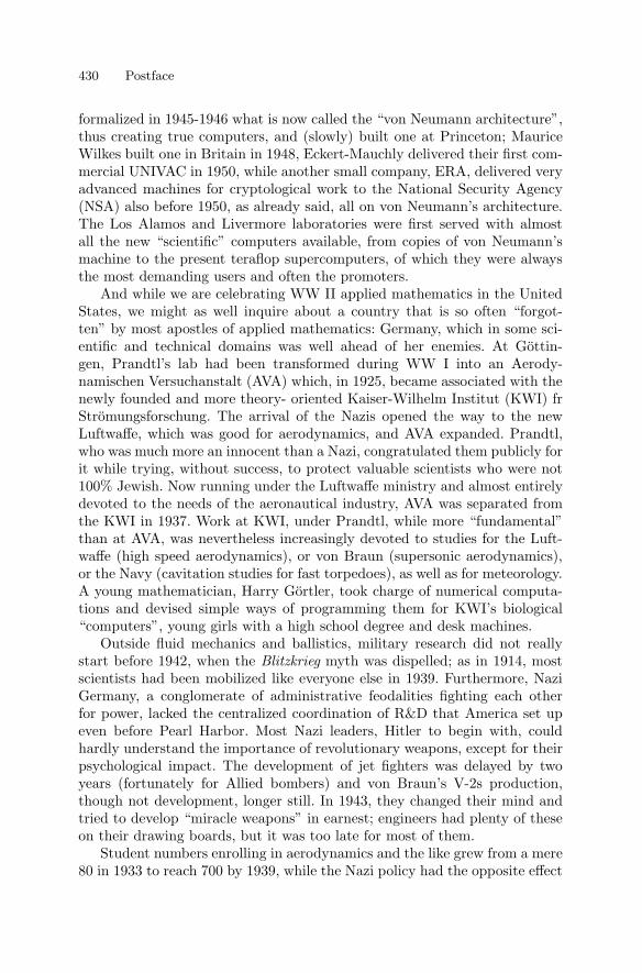
430 Postface
formalized in 1945-1946 what is now called the “von Neumann architecture”,thus creating true computers, and (slowly) built one at Princeton; MauriceWilkes built one in Britain in 1948, Eckert-Mauchly delivered their first com-mercial UNIVAC in 1950, while another small company, ERA, delivered veryadvanced machines for cryptological work to the National Security Agency(NSA) also before 1950, as already said, all on von Neumann’s architecture.The Los Alamos and Livermore laboratories were first served with almostall the new “scientific” computers available, from copies of von Neumann’smachine to the present teraflop supercomputers, of which they were alwaysthe most demanding users and often the promoters.
And while we are celebrating WW II applied mathematics in the UnitedStates, we might as well inquire about a country that is so often “forgot-ten” by most apostles of applied mathematics: Germany, which in some sci-entific and technical domains was well ahead of her enemies. At Gottin-gen, Prandtl’s lab had been transformed during WW I into an Aerody-namischen Versuchanstalt (AVA) which, in 1925, became associated with thenewly founded and more theory- oriented Kaiser-Wilhelm Institut (KWI) frStromungsforschung. The arrival of the Nazis opened the way to the newLuftwaffe, which was good for aerodynamics, and AVA expanded. Prandtl,who was much more an innocent than a Nazi, congratulated them publicly forit while trying, without success, to protect valuable scientists who were not100% Jewish. Now running under the Luftwaffe ministry and almost entirelydevoted to the needs of the aeronautical industry, AVA was separated fromthe KWI in 1937. Work at KWI, under Prandtl, while more “fundamental”than at AVA, was nevertheless increasingly devoted to studies for the Luft-waffe (high speed aerodynamics), or von Braun (supersonic aerodynamics),or the Navy (cavitation studies for fast torpedoes), as well as for meteorology.A young mathematician, Harry Gortler, took charge of numerical computa-tions and devised simple ways of programming them for KWI’s biological“computers”, young girls with a high school degree and desk machines.
Outside fluid mechanics and ballistics, military research did not reallystart before 1942, when the Blitzkrieg myth was dispelled; as in 1914, mostscientists had been mobilized like everyone else in 1939. Furthermore, NaziGermany, a conglomerate of administrative feodalities fighting each otherfor power, lacked the centralized coordination of R&D that America set upeven before Pearl Harbor. Most Nazi leaders, Hitler to begin with, couldhardly understand the importance of revolutionary weapons, except for theirpsychological impact. The development of jet fighters was delayed by twoyears (fortunately for Allied bombers) and von Braun’s V-2s production,though not development, longer still. In 1943, they changed their mind andtried to develop “miracle weapons” in earnest; engineers had plenty of theseon their drawing boards, but it was too late for most of them.
Student numbers enrolling in aerodynamics and the like grew from a mere80 in 1933 to reach 700 by 1939, while the Nazi policy had the opposite effect
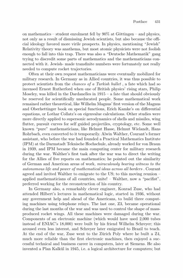
Postface 431
on mathematics – student enrolment fell by 90% at Gottingen – and physics,not only as a result of dismissing Jewish scientists, but also because the offi-cial ideology favored more virile prospects. In physics, mentioning “Jewish”Relativity theory was anathema, but most atomic physicists were not foolishenough to fall into this trap. There was also a “Deutsche Mathematik” gangtrying to discredit some parts of mathematics and the mathematicians con-nected with it. Jewish- made transfinite numbers were fortunately not reallyneeded to compute rocket trajectories.
Often at their own request mathematicians were eventually mobilized formilitary research. In Germany as in Allied countries, it was thus possible toprotect scientists from the chances of a Turkish bullet , a fate which had soincensed Ernest Rutherford when one of British physics’ rising stars, PhilipMoseley, was killed in the Dardanelles in 1915 – a fate that should obviouslybe reserved for scientifically uneducated people. Some mathematical workremained rather theoretical, like Wilhelm Magnus’ first version of the Magnusand Oberhettinger book on special functions, Erich Kamke’s on differentialequations, or Lothar Collatz’s on eigenvalue calculations. Other studies weremore directly applied to supersonic aerodynamics of shells and missiles, wingflutter, pursuit curves for self guided projectiles, cryptology, etc. Some wellknown “pure” mathematicians, like Helmut Hasse, Helmut Wielandt, HansRohrbach, even converted to it temporarily. Alwin Walther, Courant’s formerassistant, who before the war had founded a Practical Mathematics Institute(IPM) at the Darmstadt Teknische Hochschule, already worked for von Braunin 1939, and IPM became the main computing center for military researchduring the war. Walther’s first task after the war was to direct the writingfor the Allies of five reports on mathematics; he pointed out the similarityof German and American areas of work, miraculously bearing witness to theautonomous life and power of mathematical ideas across all borders . Courantagreed and invited Walther to emigrate to the US; to this moving reunion –applied mathematicians of all countries, unite! – Walther, now a “pacifist”,preferred working for the reconstruction of his country.
In Germany also, a remarkably clever engineer, Konrad Zuse, who hadattended Hilbert’s lectures in mathematical logic, started in 1936, withoutany government help and ahead of the Americans, to build three comput-ing machines using telephone relays. The last one, Z3, became operationalduring the last months of the war and was used to control the shape of mass-produced rocket wings. All these machines were damaged during the war.Components of an electronic machine (which would have used 2,000 tubesinstead of ENIAC’s 18,000) were built by his friend Wilhelm Schreyer; thisaroused even less interest, and Schreyer later emigrated to Brazil to teach.At the end of the war, Zuse went to the Zurich Poly where he built a Z4,much more reliable than the first electronic machines, then enjoyed a suc-cessful technical and business career in computers, later at Siemens. He alsoinvented a Plan Kalkul in 1945, i.e. a logical architecture for computers; but
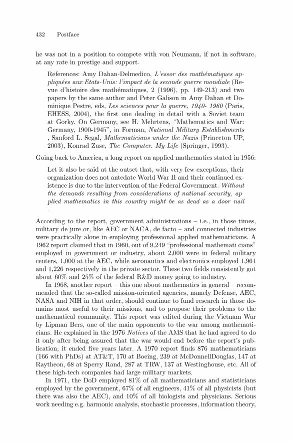
432 Postface
he was not in a position to compete with von Neumann, if not in software,at any rate in prestige and support.
References: Amy Dahan-Delmedico, L’essor des mathematiques ap-pliquees aux Etats-Unis: l’impact de la seconde guerre mondiale (Re-vue d’histoire des mathematiques, 2 (1996), pp. 149-213) and twopapers by the same author and Peter Galison in Amy Dahan et Do-minique Pestre, eds, Les sciences pour la guerre, 1940- 1960 (Paris,EHESS, 2004), the first one dealing in detail with a Soviet teamat Gorky. On Germany, see H. Mehrtens, “Mathematics and War:Germany, 1900-1945”, in Forman, National Military Establishments, Sanford L. Segal, Mathematicians under the Nazis (Princeton UP,2003), Konrad Zuse, The Computer. My Life (Springer, 1993).
Going back to America, a long report on applied mathematics stated in 1956:
Let it also be said at the outset that, with very few exceptions, theirorganization does not antedate World War II and their continued ex-istence is due to the intervention of the Federal Government. Withoutthe demands resulting from considerations of national security, ap-plied mathematics in this country might be as dead as a door nail.
According to the report, government administrations – i.e., in those times,military de jure or, like AEC or NACA, de facto – and connected industrieswere practically alone in employing professional applied mathematicians. A1962 report claimed that in 1960, out of 9,249 “professional mathemati cians”employed in government or industry, about 2,000 were in federal militarycenters, 1,000 at the AEC, while aeronautics and electronics employed 1,961and 1,226 respectively in the private sector. These two fields consistently gotabout 60% and 25% of the federal R&D money going to industry.
In 1968, another report – this one about mathematics in general – recom-mended that the so-called mission-oriented agencies, namely Defense, AEC,NASA and NIH in that order, should continue to fund research in those do-mains most useful to their missions, and to propose their problems to themathematical community. This report was edited during the Vietnam Warby Lipman Bers, one of the main opponents to the war among mathemati-cians. He explained in the 1976 Notices of the AMS that he had agreed to doit only after being assured that the war would end before the report’s pub-lication; it ended five years later. A 1970 report finds 876 mathematicians(166 with PhDs) at AT&T, 170 at Boeing, 239 at McDonnellDouglas, 147 atRaytheon, 68 at Sperry Rand, 287 at TRW, 137 at Westinghouse, etc. All ofthese high-tech companies had large military markets.
In 1971, the DoD employed 81% of all mathematicians and statisticiansemployed by the government, 67% of all engineers, 41% of all physicists (butthere was also the AEC), and 10% of all biologists and physicians. Seriouswork needing e.g. harmonic analysis, stochastic processes, information theory,
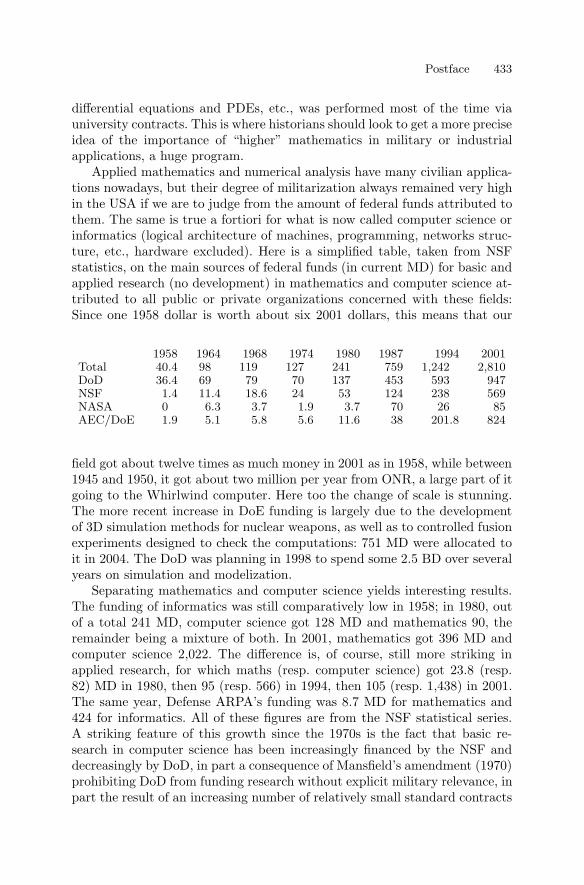
Postface 433
differential equations and PDEs, etc., was performed most of the time viauniversity contracts. This is where historians should look to get a more preciseidea of the importance of “higher” mathematics in military or industrialapplications, a huge program.
Applied mathematics and numerical analysis have many civilian applica-tions nowadays, but their degree of militarization always remained very highin the USA if we are to judge from the amount of federal funds attributed tothem. The same is true a fortiori for what is now called computer science orinformatics (logical architecture of machines, programming, networks struc-ture, etc., hardware excluded). Here is a simplified table, taken from NSFstatistics, on the main sources of federal funds (in current MD) for basic andapplied research (no development) in mathematics and computer science at-tributed to all public or private organizations concerned with these fields:Since one 1958 dollar is worth about six 2001 dollars, this means that our
1958 1964 1968 1974 1980 1987 1994 2001Total 40.4 98 119 127 241 759 1,242 2,810DoD 36.4 69 79 70 137 453 593 947NSF 1.4 11.4 18.6 24 53 124 238 569NASA 0 6.3 3.7 1.9 3.7 70 26 85AEC/DoE 1.9 5.1 5.8 5.6 11.6 38 201.8 824
field got about twelve times as much money in 2001 as in 1958, while between1945 and 1950, it got about two million per year from ONR, a large part of itgoing to the Whirlwind computer. Here too the change of scale is stunning.The more recent increase in DoE funding is largely due to the developmentof 3D simulation methods for nuclear weapons, as well as to controlled fusionexperiments designed to check the computations: 751 MD were allocated toit in 2004. The DoD was planning in 1998 to spend some 2.5 BD over severalyears on simulation and modelization.
Separating mathematics and computer science yields interesting results.The funding of informatics was still comparatively low in 1958; in 1980, outof a total 241 MD, computer science got 128 MD and mathematics 90, theremainder being a mixture of both. In 2001, mathematics got 396 MD andcomputer science 2,022. The difference is, of course, still more striking inapplied research, for which maths (resp. computer science) got 23.8 (resp.82) MD in 1980, then 95 (resp. 566) in 1994, then 105 (resp. 1,438) in 2001.The same year, Defense ARPA’s funding was 8.7 MD for mathematics and424 for informatics. All of these figures are from the NSF statistical series.A striking feature of this growth since the 1970s is the fact that basic re-search in computer science has been increasingly financed by the NSF anddecreasingly by DoD, in part a consequence of Mansfield’s amendment (1970)prohibiting DoD from funding research without explicit military relevance, inpart the result of an increasing number of relatively small standard contracts
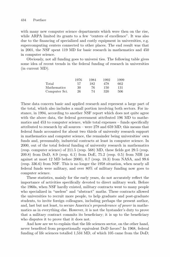
434 Postface
with many new computer science departments which were then on the rise,while ARPA limited its grants to a few “centers of excellence”. It was alsodue to the financing of specialized and costly equipment in universities, e.g.supercomputing centers connected to other places. The end result was thatin 2001, the NSF spent 119 MD for basic research in mathematics and 450in computer science.
Obviously, not all funding goes to universi ties. The following table givessome idea of recent trends in the federal funding of research in universities(in current MD).
1976 1984 1992 1999Total 57 182 478 662Mathematics 30 76 150 131Computer Sci. 26 74 320 506
These data concern basic and applied research and represent a large part ofthe total, which also includes a small portion involving both sectors. For in-stance, in 1994, according to another NSF report which does not quite agreewith the above data, the federal government attributed 196 MD to mathe-matics and 453 to computer science, while total expenses – funds specificallyattributed to research by all sources – were 278 and 659 MD; this means thatfederal funds accounted for about two thirds of university research supportin mathematics and computer science, the remainder being universities’ ownfunds and, presumably, industrial contracts at least in computer science. In2000, out of the total federal funding of university research in mathematics(resp. computer science) of 211.5 (resp. 568) MD, these fields got 29.5 (resp.209.8) from DoD, 8.9 (resp. 6.1) from DoE, 75.2 (resp. 0.5) from NIH (asagainst at most 12 MD before 2000), 0.7 (resp. 18.3) from NASA, and 99.6(resp. 336.6) from NSF. This is no longer the 1958 situation, when nearly allfederal funds were military, and over 80% of military funding now goes tocomputer science.
These statistics, mainly for the early years, do not accurately reflect theimportance of activities specifically devoted to direct military work. Beforethe 1960s, when NSF hardly existed, military contracts went to many peoplewho specialized in “useless” and “abstract” maths. These contracts allowedthe universities to recruit more people, to help graduate and post-graduatestudents, to invite foreign colleagues, including perhaps the present author,and, last but not least, to secure America’s preponderance of power in mathe-matics as in everything else. However, it is not the bystander’s duty to provethat a military contract commits its beneficiary; it is up to the beneficiarywho disputes it to prove that it does not.
And how are we to explain that the life sciences sector, on the other hand,never benefited from proportionally equivalent DoD favors? In 1968, federalfunding of life sciences totalled 1,534 MD, of which 105 came from the DoD;
Postface 435
in 1994, 9.3 BD, of which 265 MD; and in 2001, 23.057 billion in federalmoney, of which 1.052 billion from the DoD. Life sciences have been financedfor fifty years essentially by the NIH (and, to a much lesser extent, by theNSF), and very strongly encouraged by Congress and the voters. As for thedrug industry, it devotes billions to R&D without ever having received morethan a few percentage points from the federal government, less than 4% in1993 for instance. In 2001, the industry spent a total of 12.2 BD, and since itbelongs to the chemical industry sector, and the NSF tells us elsewhere thatit got 150 MD in federal funds, an upper limit of 1.4% in federal funding forthe drug industry follows. To be sure, drug companies indirectly benefit fromtheir university contracts, but their main source of R&D money is obviouslythe countless products which are sold around the world to all who can affordthem.
After students rioted against the Vietnam War and military work in uni-versities, a Congressional Mansfield’s amendment forbade the DoD from fi-nancing research without a clear military interest, as already said. It wassomewhat softened later, but its spirit remained, and military support of“pure” mathematics nearly vanished, except in cryptology. The main threatto “pure” mathematics now comes from the enormous development of appliedmathematics, even though their applications may be mostly civilian. As weshall see in the next section, this is the most striking difference betweenpost-WW II applied mathematics and Jacobi’s mathematics pour l’honneurde l’esprit humain (or for mathematicians’ entertainment...) which, to a verylarge extent, were preponderant from the 1820s to the eve of WW II.
Index
B(x, y) 95Bp(t) 205C 215C0(K) 127C0
c (X) 132Cinf(ϕ) 38Csup(ψ) 42
F (x)
∣∣∣∣ba
48
Hf (z) 302L(K) 127L(X) 132L(X, K) 132L1 norm 12L2 norm 11Linf(ϕ) 137Lsup(ψ) 137M(µ) 127MK(µ) 132Np(f) 12, 63Pf (z) 299T ′ 151Tf (ϕ) 150en(x) 19∆P 306Γ (s) 94‖µ‖ 127
‖ϕ‖(r) 148‖f‖1 12‖f‖2 11‖f‖p 12≈ 194δ(x) 112δa 150γ 215µ(n) 232
f(n) 232
f(y) 313inf(f, g) 9
∫K
f(x)dµ(x) 127(f | g) 11, 243µ(f) 127sup(f, g) 9θ(z) 319εa 150dr(ϕ, ψ) 148dm(u) 230f ϕ(x) 117f g(t) 236f(x) = O(g(x)) 171f(x) = o(g(x)) 171f(x) � g(x) 171f(x) ∼ g(x) 171f+ 9f− 9m(J) 2m(U) 44m(ϕ) 2m(f) 229m∗(f) 4m∗(f) 4zs 280T 226e(t) 226en(t) 226D(R, K) 148D 116D (T) 254D(K) 148D(R) 116H 243ϕ(k) 254lsc 40usc 42
Almost everywhere 158
Bernoulli– numbers 203– polynomials 205
Index 437
Cartesian product (measures) 131Compact support– function of 116Comparison relations 171Conjugate indices 62Convergence– dominated 16, 95– in mean 247– in mean of order p 18– in quadratic mean 18, 247Convex– function 58– set 57
Decomposition into simple elements83
Dirac sequence– on R 114– on T 241Dirichlet problem 313Distribution– derivatives of a 151– on R 147– on T 254– tempered 335Domain 274
Envelope– lower 9– upper 9Equation– integral 189– Kepler’s 185Equicontinuity 269Euler’s constant 214
Formula– Cauchy’s integral 22, 223– Euler-Maclaurin 210– Fourier inversion 322– Parseval-Bessel 20– Plancherel 323– Poisson summation 315– Stirling’s 218– Taylor’s 73– Wallis’ 70Fourier coefficients– of a distribution 255– of a function 232Fourier series– Bernoulli polynomials 265– periodic holomorphic function 282– square wave 67Fourier transform 92, 233, 313
– complex 106– of 1/(z + t)n 316– of exp(−πx2) 105– of a tempered distribution 337Function– absolutely integrable 91– absolutely integrable on X × Y 111– analytic 270– Bessel 188– convex 58– entire 282– equicontinuous 269– flat 74– Gamma 94– harmonic 306– holomorphic 271– indefinitely differentiable with rapid
decrease 330– integrable (Lebesgue) 159– integrable (Riemann) 5– lower semicontinuous 40– meromorphic 277– of compact support 116– of slow increase 257– rational 83– regulated 23– special 66– step 1– tempered 257– translated 28– upper semicontinuous 42
Gamma function– analytic continuation 108– as a limit 97– complement formula 217– definition 94– derivative 107– infinite product 216, 297– multiplication formula 112
l’Hopital’s rule 77
Inequality– Cauchy-Schwarz 10– Holder 12, 62– Minkowski 12, 62Infinite product– for the Γ function 216– of holomorphic functions 292Integral 2– absolutely convergent 91– convergent 89– double 34, 129
438 Index
– iterated 33– lower 4– of a step function 2– upper 4
Lagrange remainder 75Laplace– operator 306– transform 106Locally compact 100
Mean value 31, 228Measure– bounded 133– discrete 3– invariant 231– Lebesgue 125, 128– of an open set 44– of density µ(x) 128– of finite total mass 133– on unit circle 230– positive 127– product 131– Radon 127, 132– Stieltjes 138
Negligible– function 158– set 157Norm– L1, L2, Lp 12Norm of a measure 127
Orthogonal (functions) 12Orthogonality relations 230
Partition of unity 131Periodic function 227– mean value 228Philtre– decreasing 37– increasing 37Poisson– summation formula 315– transform 299Poles 277Primitive– of 1/(x − a) 85– of a distribution 259– of a holomorphic function 279– of a rational function 83– of a regulated function 52Principal part of order s 175Product
– convolution 117, 236– scalar 11Product of measures 131
Regularising 117Residue 279
Schwartz space– D(R) 116– D(T) 251– S(R) 330Schwarz’ lemma 275Series– asymptotic 194– complex Fourier 282– Fourier 233– hypergeometric 179– Laurent 277– Newton’s 76– power series for cot z 206– power series of a harmonic function
307– rational fractions for cot z 264– trigonometric 235Set– convex 57– integrable 166– measurable 167– negligible 157– of measure zero 157Singular point– essential 277– isolated 277Sturm-Liouville (equations) 287Subdivision 2Successive approximations 191, 289Sums– Lebesgue 126– Riemann 13
Theorem– Borel-Lebesgue 24– Cauchy 273– d’Alembert-Gauss 283– Dini 36– Dirichlet 263– Fejer 267– Fundamental (FT) 47– Lebesgue’s dominated convergence
165– Lebesgue-Fubini 108– Liouville 282– Mean value 54– Parseval-Bessel 248
Index 439
– Riesz-Fischer 162Transform– Poisson 299Translation invariance 12Truncated expansion of order s 174
Uniform continuity 28
Weierstrass’ theorems– Fourier series 242– infinite products 293– limits of holomorphic functions 291– limits of polynomials 119
Table of Contents of Volume I
Preface . . . . . . . . . . . . . . . . . . . . . . . . . . . . . . . . . . . . . . . . . . . . . . . . . . . . . . . V
I – Sets and Functions . . . . . . . . . . . . . . . . . . . . . . . . . . . . . . . . . . . . . . . . 1§1. Set Theory . . . . . . . . . . . . . . . . . . . . . . . . . . . . . . . . . . . . . . . . . . . . . . 7
1 – Membership, equality, empty set . . . . . . . . . . . . . . . . . . . . . . 72 – The set defined by a relation. Intersections and unions . . . 103 – Whole numbers. Infinite sets . . . . . . . . . . . . . . . . . . . . . . . . . . 134 – Ordered pairs, Cartesian products, sets of subsets . . . . . . . 175 – Functions, maps, correspondences . . . . . . . . . . . . . . . . . . . . . 196 – Injections, surjections, bijections . . . . . . . . . . . . . . . . . . . . . . 237 – Equipotent sets. Countable sets . . . . . . . . . . . . . . . . . . . . . . . 258 – The different types of infinity . . . . . . . . . . . . . . . . . . . . . . . . . 289 – Ordinals and cardinals . . . . . . . . . . . . . . . . . . . . . . . . . . . . . . . 31
§2. The logic of logicians . . . . . . . . . . . . . . . . . . . . . . . . . . . . . . . . . . . . . 39
II – Convergence: Discrete variables . . . . . . . . . . . . . . . . . . . . . . . . . . 45§1. Convergent sequences and series . . . . . . . . . . . . . . . . . . . . . . . . . . . 45
0 – Introduction: what is a real number? . . . . . . . . . . . . . . . . . . 451 – Algebraic operations and the order relation: axioms of R . 532 – Inequalities and intervals . . . . . . . . . . . . . . . . . . . . . . . . . . . . . 563 – Local or asymptotic properties . . . . . . . . . . . . . . . . . . . . . . . . 594 – The concept of limit. Continuity and differentiability . . . . 635 – Convergent sequences: definition and examples . . . . . . . . . . 676 – The language of series . . . . . . . . . . . . . . . . . . . . . . . . . . . . . . . 767 – The marvels of the harmonic series . . . . . . . . . . . . . . . . . . . . 818 – Algebraic operations on limits . . . . . . . . . . . . . . . . . . . . . . . . 95
§2. Absolutely convergent series . . . . . . . . . . . . . . . . . . . . . . . . . . . . . . . 989 – Increasing sequences. Upper bound of a set of real numbers 9810 – The function log x. Roots of a positive number . . . . . . . . . 10311 – What is an integral? . . . . . . . . . . . . . . . . . . . . . . . . . . . . . . . . 11012 – Series with positive terms . . . . . . . . . . . . . . . . . . . . . . . . . . . 11413 – Alternating series . . . . . . . . . . . . . . . . . . . . . . . . . . . . . . . . . . 11914 – Classical absolutely convergent series . . . . . . . . . . . . . . . . . 12315 – Unconditional convergence: general case . . . . . . . . . . . . . . . 127
442 Table of Contents of Volume I
16 – Comparison relations. Criteria of Cauchy and d’Alembert13217 – Infinite limits . . . . . . . . . . . . . . . . . . . . . . . . . . . . . . . . . . . . . . 13818 – Unconditional convergence: associativity . . . . . . . . . . . . . . 139
§3. First concepts of analytic functions . . . . . . . . . . . . . . . . . . . . . . . . . 14819 – The Taylor series . . . . . . . . . . . . . . . . . . . . . . . . . . . . . . . . . . . 14820 – The principle of analytic continuation . . . . . . . . . . . . . . . . . 15821 – The function cotx and the series
∑1/n2k . . . . . . . . . . . . . 162
22 – Multiplication of series. Composition of analytic func-tions. Formal series . . . . . . . . . . . . . . . . . . . . . . . . . . . . . . . 167
23 – The elliptic functions of Weierstrass . . . . . . . . . . . . . . . . . . 178
III – Convergence: Continuous variables . . . . . . . . . . . . . . . . . . . . . . 187§1. The intermediate value theorem . . . . . . . . . . . . . . . . . . . . . . . . . . . 187
1 – Limit values of a function. Open and closed sets . . . . . . . . 1872 – Continuous functions . . . . . . . . . . . . . . . . . . . . . . . . . . . . . . . . 1923 – Right and left limits of a monotone function . . . . . . . . . . . . 1974 – The intermediate value theorem . . . . . . . . . . . . . . . . . . . . . . . 200
§2. Uniform convergence . . . . . . . . . . . . . . . . . . . . . . . . . . . . . . . . . . . . . 2055 – Limits of continuous functions . . . . . . . . . . . . . . . . . . . . . . . . 2056 – A slip up of Cauchy’s . . . . . . . . . . . . . . . . . . . . . . . . . . . . . . . . 2117 – The uniform metric . . . . . . . . . . . . . . . . . . . . . . . . . . . . . . . . . 2168 – Series of continuous functions. Normal convergence . . . . . . 220
§3. Bolzano-Weierstrass and Cauchy’s criterion . . . . . . . . . . . . . . . . . 2259 – Nested intervals, Bolzano-Weierstrass, compact sets . . . . . 22510 – Cauchy’s general convergence criterion . . . . . . . . . . . . . . . . 22811 – Cauchy’s criterion for series: examples . . . . . . . . . . . . . . . . 23412 – Limits of limits . . . . . . . . . . . . . . . . . . . . . . . . . . . . . . . . . . . . 23913 – Passing to the limit in a series of functions . . . . . . . . . . . . 241
§4. Differentiable functions . . . . . . . . . . . . . . . . . . . . . . . . . . . . . . . . . . . 24414 – Derivatives of a function . . . . . . . . . . . . . . . . . . . . . . . . . . . . 24415 – Rules for calculating derivatives . . . . . . . . . . . . . . . . . . . . . . 25216 – The mean value theorem . . . . . . . . . . . . . . . . . . . . . . . . . . . . 26017 – Sequences and series of differentiable functions . . . . . . . . . 26518 – Extensions to unconditional convergence . . . . . . . . . . . . . . 270
§5. Differentiable functions of several variables . . . . . . . . . . . . . . . . . . 27319 – Partial derivatives and differentials . . . . . . . . . . . . . . . . . . . 27320 – Differentiability of functions of class C1 . . . . . . . . . . . . . . . 27621 – Differentiation of composite functions . . . . . . . . . . . . . . . . . 27922 - Limits of differentiable functions . . . . . . . . . . . . . . . . . . . . . 28423 – Interchanging the order of differentiation . . . . . . . . . . . . . . 28724 – Implicit functions . . . . . . . . . . . . . . . . . . . . . . . . . . . . . . . . . . 290
Table of Contents of Volume I 443
Appendix to Chapter III . . . . . . . . . . . . . . . . . . . . . . . . . . . . . . . . . . . . . 3031 – Cartesian spaces and general metric spaces . . . . . . . . . . . . . 3032 – Open and closed sets . . . . . . . . . . . . . . . . . . . . . . . . . . . . . . . . 3063 – Limits and Cauchy’s criterion in a metric space; complete
spaces . . . . . . . . . . . . . . . . . . . . . . . . . . . . . . . . . . . . . . . . . . 3084 – Continuous functions . . . . . . . . . . . . . . . . . . . . . . . . . . . . . . . . 3115 – Absolutely convergent series in a Banach space . . . . . . . . . 3136 – Continuous linear maps . . . . . . . . . . . . . . . . . . . . . . . . . . . . . . 3177 – Compact spaces . . . . . . . . . . . . . . . . . . . . . . . . . . . . . . . . . . . . . 3208 – Topological spaces . . . . . . . . . . . . . . . . . . . . . . . . . . . . . . . . . . . 322
IV – Powers, Exponentials, Logarithms, Trigonometric Func-tions . . . . . . . . . . . . . . . . . . . . . . . . . . . . . . . . . . . . . . . . . . . . . . . . . . . . . . 325§1. Direct construction. . . . . . . . . . . . . . . . . . . . . . . . . . . . . . . . . . . . . . . 325
1 – Rational exponents . . . . . . . . . . . . . . . . . . . . . . . . . . . . . . . . . . 3252 – Definition of real powers . . . . . . . . . . . . . . . . . . . . . . . . . . . . . 3273 – The calculus of real exponents . . . . . . . . . . . . . . . . . . . . . . . . 3304 – Logarithms to base a. Power functions . . . . . . . . . . . . . . . . . 3325 – Asymptotic behaviour . . . . . . . . . . . . . . . . . . . . . . . . . . . . . . . 3336 – Characterisations of the exponential, power and logarith-
mic functions . . . . . . . . . . . . . . . . . . . . . . . . . . . . . . . . . . . . 3367 – Derivatives of the exponential functions: direct method . . 3398 – Derivatives of exponential functions, powers and logarithms342
§2. Series expansions . . . . . . . . . . . . . . . . . . . . . . . . . . . . . . . . . . . . . . . . 3459 – The number e. Napierian logarithms . . . . . . . . . . . . . . . . . . . 34510 – Exponential and logarithmic series: direct method . . . . . . 34611 – Newton’s binomial series . . . . . . . . . . . . . . . . . . . . . . . . . . . . 35112 – The power series for the logarithm . . . . . . . . . . . . . . . . . . . 35913 – The exponential function as a limit . . . . . . . . . . . . . . . . . . . 36814 – Imaginary exponentials and trigonometric functions . . . . 37215 – Euler’s relation chez Euler . . . . . . . . . . . . . . . . . . . . . . . . . . . 38316 – Hyperbolic functions . . . . . . . . . . . . . . . . . . . . . . . . . . . . . . . 388
§3. Infinite products . . . . . . . . . . . . . . . . . . . . . . . . . . . . . . . . . . . . . . . . . 39417 – Absolutely convergent infinite products . . . . . . . . . . . . . . . 39418 – The infinite product for the sine function . . . . . . . . . . . . . . 39719 – Expansion of an infinite product in series . . . . . . . . . . . . . . 40320 – Strange identities . . . . . . . . . . . . . . . . . . . . . . . . . . . . . . . . . . 407
§4. The topology of the functions Arg(z) and Log z . . . . . . . . . . . . . 414
Index . . . . . . . . . . . . . . . . . . . . . . . . . . . . . . . . . . . . . . . . . . . . . . . . . . . . . . . . . 425
Universitext
Aguilar, M.; Gitler, S.; Prieto, C.: Alge-
braic Topology from a Homotopical View-point
Aksoy, A.; Khamsi, M.A.: Methods inFixed Point Theory
Alevras, D.; Padberg M.W.: Linear Opti-mization and Extensions
Andersson, M.: Topics in Complex Analysis
Aoki, M.: State Space Modeling of Time Se-ries
Arnold, V. I.: Lectures on Partial Differen-tial Equations
Audin, M.: Geometry
Aupetit, B.: A Primer on Spectral Theory
Bachem, A.; Kern, W.: Linear Program-
ming Duality
Bachmann, G.; Narici, L.; Beckenstein, E.:
Fourier and Wavelet Analysis
Badescu, L.: Algebraic Surfaces
Balakrishnan, R.; Ranganathan, K.: A
Textbook of Graph Theory
Balser, W.: Formal Power Series and Linear
Systems of Meromorphic Ordinary Differen-tial Equations
Bapat, R.B.: Linear Algebra and LinearModels
Benedetti, R.; Petronio, C.: Lectures onHyperbolic Geometry
Benth, F. E.: Option Theory with Stochas-tic Analysis
Berberian, S.K.: Fundamentals of Real
Analysis
Berger, M.: Geometry I, and II
Bliedtner, J.; Hansen, W.: Potential The-ory
Blowey, J. F.; Coleman, J. P.; Craig, A.W.(Eds.): Theory and Numerics of DifferentialEquations
Blowey, J.; Craig, A.: Frontiers in Numeri-
cal Analysis. Durham 2004
Blyth, T. S.: Lattices and Ordered AlgebraicStructures
Borger, E.; Gradel, E.; Gurevich, Y.: The
Classical Decision Problem
Bottcher, A; Silbermann, B.: Introductionto Large Truncated Toeplitz Matrices
Boltyanski, V.; Martini, H.; Soltan, P. S.:Excursions into Combinatorial Geometry
Boltyanskii, V.G.; Efremovich, V.A.: Intu-itive Combinatorial Topology
Bonnans, J. F.; Gilbert, J. C.; Lemarechal,
C.; Sagastizabal, C.A.: Numerical Opti-mization
Booss, B.; Bleecker, D.D.: Topology andAnalysis
Borkar, V. S.: Probability Theory
Brunt B. van: The Calculus of Variations
Buhlmann, H.; Gisler, A.: A Course in
Credibility Theory and Its Applications
Carleson, L.; Gamelin, T.W.: ComplexDynamics
Cecil, T. E.: Lie Sphere Geometry: WithApplications of Submanifolds
Chae, S. B.: Lebesgue Integration
Chandrasekharan, K.: Classical FourierTransform
Charlap, L. S.: Bieberbach Groups and FlatManifolds
Chern, S.: Complex Manifolds without Po-tential Theory
Chorin, A. J.; Marsden, J. E.: Mathemati-cal Introduction to Fluid Mechanics
Cohn, H.: A Classical Invitation to Alge-
braic Numbers and Class Fields
Curtis, M. L.: Abstract Linear Algebra
Curtis, M. L.: Matrix Groups
Cyganowski, S.; Kloeden, P.; Ombach, J.:From Elementary Probability to StochasticDifferential Equations with MAPLE
Dalen, D. van: Logic and Structure
Das, A.: The Special Theory of Relativity:A Mathematical Exposition
Debarre, O.: Higher-Dimensional AlgebraicGeometry
Deitmar, A.: A First Course in HarmonicAnalysis
Demazure, M.: Bifurcations and Catastro-
phes
Devlin, K. J.: Fundamentals of Contempo-
rary Set Theory
DiBenedetto, E.: Degenerate ParabolicEquations
Diener, F.; Diener, M.(Eds.): Nonstandard
Analysis in Practice
Dimca, A.: Sheaves in Topology
Dimca, A.: Singularities and Topology ofHypersurfaces
DoCarmo, M.P.: Differential Forms andApplications
Duistermaat, J. J.; Kolk, J. A.C.: LieGroups
Edwards, R. E.: A Formal Background toHigher Mathematics Ia, and Ib
Edwards, R. E.: A Formal Background toHigher Mathematics IIa, and IIb
Emery, M.: Stochastic Calculus in Mani-folds
Emmanouil, I.: Idempotent Matrices overComplex Group Algebras
Endler, O.: Valuation Theory
Erez, B.: Galois Modules in Arithmetic
Everest, G.; Ward, T.: Heights of Polyno-mials and Entropy in Algebraic Dynamics
Farenick, D.R.: Algebras of Linear Trans-formations
Foulds, L. R.: Graph Theory Applications
Franke, J.; Hardle, W.; Hafner, C.M.: Sta-tistics of Financial Markets: An Introduc-tion
Frauenthal, J. C.: Mathematical Modelingin Epidemiology
Freitag, E.; Busam, R.: Complex Analysis
Friedman, R.: Algebraic Surfaces and Holo-morphic Vector Bundles
Fuks, D.B.; Rokhlin, V.A.: Beginner’s
Course in Topology
Fuhrmann, P.A.: A Polynomial Approachto Linear Algebra
Gallot, S.; Hulin, D.; Lafontaine, J.: Rie-
mannian Geometry
Gardiner, C. F.: A First Course in Group
Theory
Garding, L.; Tambour, T.: Algebra for
Computer Science
Godbillon, C.: Dynamical Systems on Sur-faces
Godement, R.: Analysis I, and II
Goldblatt, R.: Orthogonality and Spacetime
Geometry
Gouvea, F.Q.: p-Adic Numbers
Gross, M. et al.: Calabi-Yau Manifolds andRelated Geometries
Gustafson, K. E.; Rao, D.K.M.: NumericalRange. The Field of Values of Linear Oper-ators and Matrices
Gustafson, S. J.; Sigal, I.M.: MathematicalConcepts of Quantum Mechanics
Hahn, A. J.: Quadratic Algebras, CliffordAlgebras, and Arithmetic Witt Groups
Hajek, P.; Havranek, T.: Mechanizing Hy-pothesis Formation
Heinonen, J.: Lectures on Analysis on Met-ric Spaces
Hlawka, E.; Schoißengeier, J.; Taschner,R.: Geometric and Analytic Number The-ory
Holmgren, R.A.: A First Course in DiscreteDynamical Systems
Howe, R., Tan, E.Ch.: Non-Abelian Har-monic Analysis
Howes, N.R.: Modern Analysis and Topol-ogy
Hsieh, P.-F.; Sibuya, Y. (Eds.): Basic The-ory of Ordinary Differential Equations
Humi, M., Miller, W.: Second Course in Or-dinary Differential Equations for Scientistsand Engineers
Hurwitz, A.; Kritikos, N.: Lectures onNumber Theory
Huybrechts, D.: Complex Geometry: An In-troduction
Isaev, A.: Introduction to MathematicalMethods in Bioinformatics
Istas, J.: Mathematical Modeling for theLife Sciences
Iversen, B.: Cohomology of Sheaves
Jacod, J.; Protter, P.: Probability Essen-tials
Jennings, G.A.: Modern Geometry withApplications
Jones, A.; Morris, S. A.; Pearson, K.R.:Abstract Algebra and Famous Inpossibili-ties
Jost, J.: Compact Riemann Surfaces
Jost, J.: Dynamical Systems. Examples of
Complex Behaviour
Jost, J.: Postmodern Analysis
Jost, J.: Riemannian Geometry and Geo-metric Analysis
Kac, V.; Cheung, P.: Quantum Calculus
Kannan, R.; Krueger, C.K.: Advanced
Analysis on the Real Line
Kelly, P.; Matthews, G.: The Non-Euclidean Hyperbolic Plane
Kempf, G.: Complex Abelian Varieties andTheta Functions
Kitchens, B. P.: Symbolic Dynamics
Kloeden, P.; Ombach, J.; Cyganowski, S.:From Elementary Probability to StochasticDifferential Equations with MAPLE
Kloeden, P. E.; Platen; E.; Schurz, H.: Nu-merical Solution of SDE Through ComputerExperiments
Kostrikin, A. I.: Introduction to Algebra
Krasnoselskii, M.A.; Pokrovskii, A.V.:Systems with Hysteresis
Kurzweil, H.; Stellmacher, B.: The Theory
of Finite Groups. An Introduction
Lang, S.: Introduction to DifferentiableManifolds
Luecking, D.H., Rubel, L.A.: ComplexAnalysis. A Functional Analysis Approach
Ma, Zhi-Ming; Roeckner, M.: Introductionto the Theory of (non-symmetric) DirichletForms
Mac Lane, S.; Moerdijk, I.: Sheaves in
Geometry and Logic
Marcus, D.A.: Number Fields
Martinez, A.: An Introduction to Semiclas-sical and Microlocal Analysis
Matousek, J.: Using the Borsuk-Ulam The-orem
Matsuki, K.: Introduction to the Mori Pro-gram
Mazzola, G.; Milmeister G.; Weissman J.:Comprehensive Mathematics for ComputerScientists 1
Mazzola, G.; Milmeister G.; Weissman J.:Comprehensive Mathematics for ComputerScientists 2
Mc Carthy, P. J.: Introduction to Arith-metical Functions
McCrimmon, K.: A Taste of Jordan Alge-bras
Meyer, R.M.: Essential Mathematics forApplied Field
Meyer-Nieberg, P.: Banach Lattices
Mikosch, T.: Non-Life Insurance Mathe-
matics
Mines, R.; Richman, F.; Ruitenburg, W.: ACourse in Constructive Algebra
Moise, E. E.: Introductory Problem
Courses in Analysis and Topology
Montesinos-Amilibia, J.M.: Classical Tes-sellations and Three Manifolds
Morris, P.: Introduction to Game Theory
Nikulin, V.V.; Shafarevich, I. R.: Geome-tries and Groups
Oden, J. J.; Reddy, J. N.: Variational Meth-ods in Theoretical Mechanics
Øksendal, B.: Stochastic Differential Equa-tions
Øksendal, B.; Sulem, A.: Applied Stochas-tic Control of Jump Diffusions
Poizat, B.: A Course in Model Theory
Polster, B.: A Geometrical Picture Book
Porter, J. R.; Woods, R.G.: Extensions andAbsolutes of Hausdorff Spaces
Radjavi, H.; Rosenthal, P.: SimultaneousTriangularization
Ramsay, A.; Richtmeyer, R.D.: Introduc-tion to Hyperbolic Geometry
Rees, E.G.: Notes on Geometry
Reisel, R. B.: Elementary Theory of MetricSpaces
Rey, W. J. J.: Introduction to Robust andQuasi-Robust Statistical Methods
Ribenboim, P.: Classical Theory of Alge-braic Numbers
Rickart, C. E.: Natural Function Algebras
Roger G.: Analysis II
Rotman, J. J.: Galois Theory
Rubel, L.A.: Entire and Meromorphic Func-tions
Ruiz-Tolosa, J. R.; Castillo E.: From Vec-tors to Tensors
Runde, V.: A Taste of Topology
Rybakowski, K. P.: The Homotopy Indexand Partial Differential Equations
Sagan, H.: Space-Filling Curves
Samelson, H.: Notes on Lie Algebras
Schiff, J. L.: Normal Families
Sengupta, J.K.: Optimal Decisions under
Uncertainty
Seroul, R.: Programming for Mathemati-cians
Seydel, R.: Tools for Computational Fi-
nance
Shafarevich, I. R.: Discourses on Algebra
Shapiro, J. H.: Composition Operators andClassical Function Theory
Simonnet, M.: Measures and Probabilities
Smith, K. E.; Kahanpaa, L.; Kekalainen,P.; Traves, W.: An Invitation to AlgebraicGeometry
Smith, K.T.: Power Series from a Compu-
tational Point of View
Smorynski, C.: Logical Number Theory I.An Introduction
Stichtenoth, H.: Algebraic Function Fieldsand Codes
Stillwell, J.: Geometry of Surfaces
Stroock, D.W.: An Introduction to the The-ory of Large Deviations
Sunder, V. S.: An Invitation to von Neu-mann Algebras
Tamme, G.: Introduction to Etale Coho-
mology
Tondeur, P.: Foliations on RiemannianManifolds
Toth, G.: Finite Mobius Groups, Minimal
Immersions of Spheres, and Moduli
Verhulst, F.: Nonlinear Differential Equa-tions and Dynamical Systems
Wong, M.W.: Weyl Transforms
Xambo-Descamps, S.: Block Error-Cor-recting Codes
Zaanen, A.C.: Continuity, Integration andFourier Theory
Zhang, F.: Matrix Theory
Zong, C.: Sphere Packings
Zong, C.: Strange Phenomena in Convexand Discrete Geometry
Zorich, V.A.: Mathematical Analysis I
Zorich, V.A.: Mathematical Analysis II


![[Godement R.] Algebra(Bookos.org)](https://img.pdfslide.net/doc/110x75/55cf9a8f550346d033a25541/godement-r-algebrabookosorg.jpg)