Embed Size (px)
Citation preview
Diss. ETH No. 17354
Role-based Configuration of WirelessSensor Networks
A dissertation submitted toETH Zurich
for the degree ofDoctor of Sciences
presented byChristian Frank
Diplom-Informatiker, Technische Universität Berlinborn November 3rd, 1978
citizen of Germany
accepted on the recommendation ofProf. Dr. Friedemann Mattern, examiner
Prof. Dr. Gian Pietro Picco, co-examiner
2007

ii

Abstract
Wireless sensor networks consist of so-called sensor nodes – small com-puting devices which integrate processing, storage, sensing, and wirelesscommunication capabilities and an autonomous power source. Due totheir decreased dependency on a wired infrastructure, wireless sensor net-works can be used to monitor environmental phenomena on an unprece-dented scale.
This thesis considers approaches for in-situ configuration of wirelesssensor networks. In-situ configuration is a prominent challenge of wire-less sensor networks: On the one hand, network nodes typically cannotbe configured manually due to the large scale of such networks. On theother hand, nodes cannot be configured automatically prior to deploy-ment because their runtime properties are unknown at deployment timeand node failures (e.g., due to depleted battery power) require frequentre-configuration of the network during its lifetime.
Consequently, it is common that, right after deployment, a wireless sen-sor network is in a homogeneous software state. In this property, wire-less sensor networks differ from classic infrastructure-based networks inwhich some nodes are custom-built or pre-configured for a certain task(e.g., a router used for routing). Therefore, a main purpose of config-uration is to break the initial symmetry and to realize and maintain thedesired structure of the network in face of runtime properties that changewith time.
The contributions of this thesis approach such configuration tasks byassigning roles to network nodes based on their runtime properties (i.e.,based on the nodes’ remaining battery power, location, or network neigh-bors). Such automatic role-based network configuration is part of manyapplications and also present in classic configuration protocols developedfor wireless sensor networks. For example, the coverage problem aimsto exploit redundancy in the network by assigning the roles sensing andidle such that the selected sensing nodes suffice to collect data on thearea of interest. Similarly, clustering aproaches select cluster leaders assole communication partners for slave nodes in their vicinity which al-

iv Abstract
lows slave nodes to save energy by synchronizing to the communicationschedule of their cluster leaders. Finally, the construction of a data gath-ering tree made up of adequately chosen aggregator nodes can also beinterpreted as a role-based configuration problem.
In this context, this thesis claims that generic system support for suchrole-based configuration tasks can significantly reduce the effort requiredfor programming wireless sensor network applications and yet be imple-mented efficiently. We sustain this claim by providing generic supportfor role-based configuration problems occuring in a set of heterogeneousapplication domains and by showing that in each domain adequate sys-tem support can significantly simplify the configuration of an application.Further, our evaluations demonstrate that the involved overhead is propor-tional to the “hardness” of the task that is formulated by the programmerat the provided configuration interface. The observed overhead is some-times even comparable to application-specific implementations that havebeen optimized for the specific configuration task.
In a wider context, this thesis’ contributions provide advances towardplug and play sensor network systems that can be flexibly parameterizedfor a certain application-specific task without requiring the expertise of ahighly specialized engineer for this purpose. Such out of the box usabil-ity, often presumed a key prerequisite to wide-spread usage of wirelesssensor networks, would finally enable the economies of scale commonlyassociated with the wireless sensor network vision.

Kurzfassung
Drahtlose Sensornetze basieren auf miteinander kommunizierenden Sen-sorknoten, die auf engem Raum einen Mikroprozessor, Speicherplatz, ei-ne autonome Energiequelle und die Möglichkeit zur drahtlosen Kommu-nikation vereinen. Da Sensornetze nicht von vorhandener Infrastrukturabhängig sind, können sie Umweltphänomene kostengünstiger und gross-flächiger als bestehende Methoden erfassen.
Diese Arbeit beschäftigt sich mit der Konfiguration von bereits in ei-ner Arbeitsumgebung installierten Sensornetzen. Solche Konfigurationder Sensorknoten vor Ort ist häufig unumgänglich: Einerseits können we-gen der zu erwartenden Grösse solcher Netze die einzelnen Sensorkno-ten nicht manuell konfiguriert werden, andererseits kann die automatischeKonfiguration der Knoten erst nach deren Installation erfolgen, da die fürdie Konfiguration erforderlichen Knoteneigenschaften (wie zum Beispielderen Ort) erst zur Laufzeit des Systems bekannt sind. Zudem verlangenhäufig auftretende Ausfälle einzelner Knoten, bedingt durch Umweltein-flüsse oder aufgebrauchte Batteriekapazität, Anpassungen in der Konfigu-ration der Knoten während des laufenden Betriebs.
Deshalb befinden sich die Knoten eines Sensornetzes direkt nach des-sen Inbetriebnahme zunächst in einem homogenen Zustand. In dieser Ei-genschaft unterscheiden sich Sensornetze von klassischen infrastruktur-basierten Computernetzen, in denen Knoten entweder für eine bestimmteAufgabe (zum Beispiel, um Nachrichten weiterzuleiten) gebaut wurdenoder zumindest vor der Inbetriebnahme auf eine bestimmte Aufgabe hinvorkonfiguriert werden können. Ein Hauptaugenmerk bei der Konfigurati-on von Sensornetzen muss deshalb sein, den anfänglichen symmetrischenZustand in die gewünschte Struktur des Netzes zu überführen und dieseStruktur trotz Änderungen der Knoteneigenschaften über die Laufzeit desNetzes hinweg aufrechtzuerhalten.
Diese Disseration nimmt sich Konfigurationsaufgaben in Sensornetzenan, indem sie Sensorknoten, basierend auf deren Eigenschaften (wie zumBeispiel deren Ort, deren verbleibende Batteriekapazität oder Eigenschaf-ten der jeweiligen Nachbarn in der Kommunikationstopologie), Rollen

vi Kurzfassung
zuweist. Solche automatische Konfiguration mittels Zuweisung von Rol-len ist Teil vieler klassischer Konfigurationsprotokolle, die für drahtlo-se Sensornetze entwickelt wurden. Zum Beispiel hat das sogenannte Co-verage-Problem zum Ziel, die Redundanz von Sensorknoten zu nutzen:Die Rolle Sensor an wird an eine Untermenge aller Knoten zugewiesen,die für die Abdeckung des untersuchten Gebietes ausreicht, wohingegendie Knoten mit der Rolle Sensor aus in einen energiesparenden Zustandwechseln können. Ähnlich wird im Clustering-Problem ein Knoten alsZentrum einer Gruppe von Knoten ausgewählt, während die verbleiben-den Randknoten Energie einsparen, indem sie nur mit dem ihnen zugewie-senen Zentrum kommunizieren und daher keine Nachrichten für andereKnoten weiterleiten müssen. Schliesslich lassen sich auch Baumstruktu-ren, die häufig zur Datengewinnung in Sensornetzen verwendet werden,auch als Rollenzuweisungsproblem interpretieren.
In diesem Zusammenhang vertrete ich in dieser Arbeit die These, dassgenerische Systemunterstützung für rollenbasierte Konfiguration die Pro-grammierung von Applikationen für drahtlose Sensornetze beträchtlichvereinfacht und dass solche Unterstützung auch effizient implementiertwerden kann. Diese These wird durch die Bereitstellung verschiedenerrollenbasierter Konfigurationsdienste gestützt, welche in ihrer jeweiligenAnwendungsdomäne die Lösung von Konfigurationsaufgaben signifikanterleichtern. In Experimenten wird aufgezeigt, wie der Kommunikations-aufwand der bereitgestellten Dienste sich proportional zur “Schwere” desvom Programmierer spezifizierten Konfigurationsproblems verhält. Zu-dem erfordern die generischen Dienste häufig nicht mehr Aufwand alsDienste, die auf spezifische Applikationen hin optimiert wurden.
In einem weiter gefassten Kontext kann diese Dissertation als ein Bau-stein auf dem Weg zu komponentenbasierten Sensornetzsystemen ange-sehen werden, in denen eine gewünschte Applikation aus bestehendenDiensten flexibel zusammengesetzt werden kann, ohne dass die Hilfe ei-nes Spezialisten dafür nötig wäre. Solch einfache Nutzbarkeit von Sen-sornetztechnologien wird oft als eine Schlüsselvoraussetzung für die An-wendung von Sensornetzen in Fachgebieten ausserhalb der Informatik an-gesehen. Eine grössere Verbreitung von Sensornetzen würde wiederumauch die häufig genannte Vision der Massenproduktion von Sensorknotenund die damit verbundene Wirtschaftlichkeit grosser Sensornetze näherrücken lassen.

Contents
List of Figures xii
1 Introduction 11.1 Motivation . . . . . . . . . . . . . . . . . . . . . . . . . 11.2 Generic Role Assignment . . . . . . . . . . . . . . . . . 31.3 Distributed Facility Location . . . . . . . . . . . . . . . 51.4 Query Scoping . . . . . . . . . . . . . . . . . . . . . . 61.5 Background . . . . . . . . . . . . . . . . . . . . . . . . 8
1.5.1 Programming Frameworks . . . . . . . . . . . . 81.5.2 Configuration Algorithms . . . . . . . . . . . . 131.5.3 Task Assignment . . . . . . . . . . . . . . . . . 141.5.4 Resource Allocation . . . . . . . . . . . . . . . 15
1.6 Summary . . . . . . . . . . . . . . . . . . . . . . . . . 161.7 Outline . . . . . . . . . . . . . . . . . . . . . . . . . . 17
2 Generic Role Assignment 192.1 Overview . . . . . . . . . . . . . . . . . . . . . . . . . 202.2 Related Work . . . . . . . . . . . . . . . . . . . . . . . 232.3 Role Specifications . . . . . . . . . . . . . . . . . . . . 25
2.3.1 Application Examples . . . . . . . . . . . . . . 252.3.2 Syntax and Semantics . . . . . . . . . . . . . . 27
2.4 Distributed Role Assignment Algorithms . . . . . . . . 302.4.1 Overview . . . . . . . . . . . . . . . . . . . . . 312.4.2 Initialization . . . . . . . . . . . . . . . . . . . 312.4.3 Property Propagation . . . . . . . . . . . . . . . 332.4.4 Local Rule Evaluation . . . . . . . . . . . . . . 352.4.5 Property and Network Dynamics . . . . . . . . . 362.4.6 Termination . . . . . . . . . . . . . . . . . . . . 372.4.7 Probabilistic Initialization . . . . . . . . . . . . 39
2.5 Development Environment . . . . . . . . . . . . . . . . 432.6 Evaluation . . . . . . . . . . . . . . . . . . . . . . . . . 462.7 Qualitative Comparison . . . . . . . . . . . . . . . . . . 54
viii Contents
2.8 Role Assignment Solver . . . . . . . . . . . . . . . . . 562.8.1 Integer Program Mapping . . . . . . . . . . . . 572.8.2 Evaluation . . . . . . . . . . . . . . . . . . . . 66
2.9 Additional Role Specifications and Language Extensions 712.10 Summary . . . . . . . . . . . . . . . . . . . . . . . . . 78
3 Distributed Facility Location 813.1 Model and Applications . . . . . . . . . . . . . . . . . . 833.2 Related Work . . . . . . . . . . . . . . . . . . . . . . . 863.3 Centralized Algorithms . . . . . . . . . . . . . . . . . . 873.4 One-hop Approximation . . . . . . . . . . . . . . . . . 893.5 Multi-hop Approximation . . . . . . . . . . . . . . . . . 933.6 Evaluation . . . . . . . . . . . . . . . . . . . . . . . . . 97
3.6.1 Scalability . . . . . . . . . . . . . . . . . . . . 973.6.2 Network Dynamics . . . . . . . . . . . . . . . . 102
3.7 Summary . . . . . . . . . . . . . . . . . . . . . . . . . 105
4 Query Scoping 1074.1 The Object Localization Application . . . . . . . . . . . 1084.2 Related Work . . . . . . . . . . . . . . . . . . . . . . . 1104.3 System Architecture . . . . . . . . . . . . . . . . . . . . 113
4.3.1 Sensing Functionality . . . . . . . . . . . . . . 1144.3.2 Application Specific Services . . . . . . . . . . 115
4.4 Query Services . . . . . . . . . . . . . . . . . . . . . . 1164.4.1 Query Service Interface . . . . . . . . . . . . . 1164.4.2 Query Scoping Algorithm . . . . . . . . . . . . 1194.4.3 Example Parameterizations . . . . . . . . . . . . 1214.4.4 Discussion . . . . . . . . . . . . . . . . . . . . 1294.4.5 Global Query Service . . . . . . . . . . . . . . . 131
4.5 Privacy Considerations . . . . . . . . . . . . . . . . . . 1334.6 Evaluation . . . . . . . . . . . . . . . . . . . . . . . . . 135
4.6.1 Real-world Experiment . . . . . . . . . . . . . . 1364.6.2 Simulation Model . . . . . . . . . . . . . . . . 1374.6.3 Simulation Results . . . . . . . . . . . . . . . . 141
4.7 Summary . . . . . . . . . . . . . . . . . . . . . . . . . 149
5 Conclusion 1515.1 Contributions . . . . . . . . . . . . . . . . . . . . . . . 151
5.1.1 Generic Role Assignment . . . . . . . . . . . . 151
Contents ix
5.1.2 Facility Location . . . . . . . . . . . . . . . . . 1525.1.3 Query Scoping . . . . . . . . . . . . . . . . . . 152
5.2 Limitations . . . . . . . . . . . . . . . . . . . . . . . . 1535.2.1 Generic Role Assignment . . . . . . . . . . . . 1535.2.2 Distributed Facility Location . . . . . . . . . . . 1545.2.3 Query Scoping . . . . . . . . . . . . . . . . . . 155
5.3 Outlook . . . . . . . . . . . . . . . . . . . . . . . . . . 1565.3.1 Generic Role Assignment . . . . . . . . . . . . 1565.3.2 Distributed Facility Location . . . . . . . . . . . 1575.3.3 Query Scoping . . . . . . . . . . . . . . . . . . 1585.3.4 A Comprehensive Configuration Framework . . 158
5.4 Concluding Remarks . . . . . . . . . . . . . . . . . . . 161
Bibliography 162

x Contents

List of Figures
1.1 Classes of background literature . . . . . . . . . . . . . 9
2.1 Core elements of generic role assignment . . . . . . . . 202.2 Node A after initialization . . . . . . . . . . . . . . . . 322.3 Property propagation and local rule evaluation . . . . . . 342.4 Sample cache table at node B . . . . . . . . . . . . . . . 352.5 Propagation wave . . . . . . . . . . . . . . . . . . . . . 422.6 Role assignment simulation tool . . . . . . . . . . . . . 442.7 Simulation parameters . . . . . . . . . . . . . . . . . . 452.8 Sent messages per node with increasing density . . . . . 482.9 Percentage of incorrect assignments from total nodes with
increasing density . . . . . . . . . . . . . . . . . . . . . 502.10 Robustness in face of dropped packets . . . . . . . . . . 522.11 Total role changes per node with increasing density . . . 532.12 Coverage application with increasing scope . . . . . . . 542.13 Set equality . . . . . . . . . . . . . . . . . . . . . . . . 642.14 The number of variables required for modeling set equal-
ity depends on the specified scopes . . . . . . . . . . . . 652.15 Number of ON nodes in simplified coverage example . . 672.16 Original clustering specification . . . . . . . . . . . . . 682.17 Clustering results on a 9x9 grid, minimizing vs. maximiz-
ing clusterheads and gateways (clusterheads are black,gateways are yellow, slaves are white, and edges betweengateways and their clusterheads are emphasized) . . . . . 68
2.18 RED / GREEN example: None of the four possible roleassignments satisfies the role specification . . . . . . . . 70
2.19 Connected clustering specification . . . . . . . . . . . . 732.20 Clustered tree specification . . . . . . . . . . . . . . . . 73
3.1 Effects of different opening cost parameters; D(sink, i)denotes the shortest-path distance to the sink, which islocated in the upper left corner . . . . . . . . . . . . . . 84
3.2 Performance of one-hop and multi-hop algorithms . . . . 99
xii List of Figures
3.3 Average scope size vs. total runtime (in rounds). In Fig-ure 3.3(b) the error bars denote the maximum and theminimum that occurred. . . . . . . . . . . . . . . . . . . 101
3.4 Deployment plan, network topology, and computed con-figuration . . . . . . . . . . . . . . . . . . . . . . . . . 103
3.5 Solutions’ optimality over time . . . . . . . . . . . . . . 104
4.1 User issues an object search query . . . . . . . . . . . . 1094.2 System architecture . . . . . . . . . . . . . . . . . . . . 1134.3 Example Data model . . . . . . . . . . . . . . . . . . . 1184.4 Example search tree generated by three relation types . . 1224.5 Example strategy and scoping results with different limits
on the number of queried sensors qmax. Sensors in scopeare marked with black dots. . . . . . . . . . . . . . . . . 124
4.6 A search strategy based on the location of the last reportand its neighborhood . . . . . . . . . . . . . . . . . . . 125
4.7 Search strategy taking the order of neighboring locationsinto account . . . . . . . . . . . . . . . . . . . . . . . . 127
4.8 A combined search strategy (the search scope is expandedin four steps) . . . . . . . . . . . . . . . . . . . . . . . 128
4.9 Experiment setup: Average reply times (in seconds) forthe 10 tagged objects in different rooms . . . . . . . . . 136
4.10 Environment models . . . . . . . . . . . . . . . . . . . 1394.11 Success rate and overhead with different positioning tech-
nologies . . . . . . . . . . . . . . . . . . . . . . . . . . 1434.12 Cumulative density functions of reply times . . . . . . . 1444.13 Varying sensing range and mobility . . . . . . . . . . . 1454.14 Cell-based scoping with varying user density . . . . . . 1474.15 Overhead of the experiments shown in Figure 4.14 . . . 148
1 Introduction
Wireless sensor networks consist of so-called sensor nodes – small un-tethered computing devices equipped with sensors, a wireless radio, aprocessor, and autonomous power supply. Large and dense networks ofthese devices can be deployed unobtrusively in the physical environmentin order to monitor a wide variety of real-world phenomena with unprece-dented quality and scale while only marginally disturbing the observedphysical processes [ASSC02, KW05].
Various research projects have involved wireless sensor network de-ployments. These include examining the nesting behavior of otherwiseelusive seabirds [MPS+02], monitoring the micro-climate of redwoodtrees [TPS+05], observing the structural integrity of bridges [XRC+04],and assisting firefighters and help workers with real-time information ontheir current environment [LMFJ+04].
Each of the deployments, however, has required considerable program-ming and maintenance effort by highly-specialized engineers and re-searchers working in the sensor network field. Key for the wide-spreadapplicability of wireless sensor networks, however, is that non-experts caneasily set up a network for a task at hand. To achieve this, system sup-port for the core issues that re-appear in many wireless sensor networkapplications must be available, in order to provide non-experts high-levellevers for specifying the network’s behavior.
In this context, the aim of this thesis is to provide specification tech-niques, algorithms, and tools to support developers with one commonneed that re-appears in applications for large-scale wireless sensor net-works: The configuration of the nodes in the network.
1.1 Motivation
Configuration is a prominent challenge in wireless sensor networks basedon an intrinsic property in which these networks differ from traditionaldistributed systems. In classic infrastructure-based networks, many nodesare manufactured and installed with a certain purpose (such as a router,
2 Chapter 1. Introduction
a hub, a server, or a client device). Typically, the nodes’ physical loca-tion and their place in the communication topology are pre-determined ormanually assigned by network administrators. Moreover, single purposedevices, such as routers, come with pre-installed software dedicated toperforming the specific task. Multi-purpose devices, such as servers orclients, can also be set up by hand or in batches by a network administra-tor who distributes software to a number of nodes from a central location.
In contrast, in wireless sensor networks, many node properties on whichconfiguration decisions are regularly based either cannot be known in ad-vance or change with time. One such property is the nodes’ physical lo-cation: Some applications require that nodes are deployed at random, i.e.,dropped out of the air to the areas of interest [CHP+04]. Others involvemobile sensors attached to animals [JOW+02, BLM05] or carried by peo-ple [EAL+06, FBRK07]. Similar considerations apply to other runtimeproperties such as the nodes’ battery power or the quality of their mea-surements. Moreover, node failures are common as nodes may becomedysfunctional due to depleted battery power or environmental damage.
Based on these observations, a sensor node cannot specialize on a cer-tain task before the network is in operation. Instead, the network starts outin a homogeneous software state and the configuration of the network, interms of specialized roles such as clients, hubs, routers and servers, mustbe computed and maintained based on the network’s runtime parameters.
This thesis provides system support for such in-situ configuration ofwireless sensor networks. First, a generic framework which allows to statethe desired network structure by means of a simple declarative interfaceis presented together with efficient algorithms for its implementation.
The interface of the presented framework allows programmers to for-mulate a variety of network configuration problems focusing on ease ofuse for application-domain experts. In this regard, the provided interfacecannot express every conceivable configuration task.
Therefore, we also elaborate on two specific configuration problemswhich require more advanced features. The first approach supports de-velopers with computing near-optimal clustering configurations, whichinvolve selecting a few nodes as hubs providing certain services to theirnetwork neighbors. The second approach supports developers with a spe-cific form of the coverage problem by selecting a set of nodes, which arelikely to provide useful data on a phenomenon of interest, as data sources,while the remaining nodes may keep their sensors off and thus save power.
We detail each of these contributions in the following three sections.
1.2. Generic Role Assignment 3
1.2 Generic Role Assignment
In Chapter 2, we present a programming framework concerned with as-signing specific roles to individual sensor nodes if certain conditions aremet. These conditions can be formulated in terms of runtime propertiesof a node (e.g., its location or battery level) and in terms of properties ofnodes in the network neighborhood [RFMB04, FR05]. As the networkand node properties change over time, role assignments must be updatedto reflect these changes. Based on the assigned roles, sensor nodes mayadapt their behavior accordingly, establish cooperation with other nodes,or even download specific code for the selected role.
A number of research projects have stated the need for such role-based configuration in sensor networks (e.g., [HMCP04, MLM+05,UWMG05]). Moreover, even classic network configuration problems canbe considered instances of generic role assignment. To illustrate the con-cept consider the coverage problem [XHE01]. Here, two roles on andoff are defined such that every geographic spot falls within the observa-tion range of at least one on node. Based on this definition, off nodes donot contribute to sensor coverage and thus may switch to a power-savingsleep mode. Once an on node fails, e.g., due to depleted battery power,redundant off nodes would switch their role to on such that the coveragecondition is satisfied.
Similar roles and conditions for their assignment can be found for othernetwork configuration problems. For example, to obtain a clustered con-figuration [KG02], the roles clusterhead and slave are assigned toeach node such that clusterheads can act as hubs and represent sole com-munication partners for associated slave nodes, while gateway nodesforward data between clusterheads. Similarly, a data aggregation tree canbe implemented by assigning the roles source and aggregator in amanner that allows aggregators to efficiently compress the data providedby source nodes while forwarding it to the network base station.
While a number of specialized algorithms for these problems havebeen developed, these are typically hard to adapt to different applica-tions, where varying criteria for assigning the above roles may have tobe applied. Driven by these observations, the presented role assignmentframework provides specification techniques and algorithms that supportgeneric role assignment, a programming abstraction applicable to a widevariety of role-assignment problems similar to the ones described above.

4 Chapter 1. Introduction
Moreover, the results of our work may be integrated as a fundamentalservice into programming frameworks such as [HMCP04, MLM+05].
Generic role assignment can be considered a programming abstractionthat partially shields application developers from the complexity of pro-gramming sensor networks at the system level. Rather than implementinglow-level protocols and node functions, the developer can now specifyparts of the system behavior using a high-level configuration language.Such programming abstractions have recently gained significant attention(e.g., [ABC+04, WM04]) and can be interpreted as a step towards mak-ing sensor networks more accessible for users who are not experiencedsystem-level programmers (e.g., typical application-domain experts).
The presented role assignment framework consists of three elements.To configure a sensor network, the programmer may issue a set of rolespecifications containing a set of roles and conditions for their assign-ment. At the network base station, a role compiler translates the speci-fication into a compact abstract representation. This representation maybe either pre-installed on sensor nodes prior to deployment or injectedinto the network by the network base station. On the nodes, a propertydirectory provides transparent access to node properties and capabilitiessuch as a node’s location or remaining battery power. Based on the nodes’properties and a given specification, a decentralized role assignment algo-rithm assigns roles to sensor nodes. The assignment of a given role maythen trigger role-specific code to be executed, for example, enabling acertain routing component once the node has become clusterhead ortrigger a download of additional role-specific code from the network basestation. Finally, the role compiler has been enhanced with a tool for offlinespecification analysis [FR06] which allows to examine various aspects ofrole specifications, such as feasibility and optimality, before distributingthem to the network.
In our evaluation, we show that the overhead induced by the distributedrole assignment algorithm is small and moreover proportional to the hard-ness of the specified configuration problem. Moreover, we discuss howthe semantics of role specifications executed by our generic algorithmsare comparable to highly specialized algorithms designed for the sameproblems. Finally, we demonstrate how offline specification analysis canprovide further valuable insights into the runtime behavior of certain rolespecifications.

1.3. Distributed Facility Location 5
1.3 Distributed Facility Location
The general focus of generic role assignment is more on ease of use thanon computing an optimized configuration. In particular, while the dis-tributed role assignment algorithms attempt to find a feasible configura-tion based on a given role specification, they do not employ any meansfor choosing an optimal role assignment (for example, with a minimumnumber of clusterhead nodes) among multiple assignments that arefeasible.
We therefore examine an important subclass of role-assignment prob-lems for which optimality guarantees can be provided in Chapter 3. Thissubclass requires that certain nodes are selected as servers such that ev-ery network node can access a server node within a (preferably) smallnetwork distance from itself. Several application examples mentioned inthe previous section belong to this class, for example clustering and ag-gregator placement. We use the facility location problem to model suchnetwork configuration decisions which require choosing a subset of servernodes (also known as facilities) to act as service providers for their net-work neighborhood (the remaining nodes are called clients).
The facility location problem deals with finding an optimal trade-offbetween two different costs of network operation. On the one hand, so-called opening costs model the costs for operating server nodes. For ex-ample, these may represent a node’s increased communication load if itwere to forward traffic for its neighbors or, generally, a measure of thenode’s suitability as a clusterhead or service provider. On the other hand,communication costs model the overhead involved when clients commu-nicate with their closest server, for example, based on the quality of theobserved network paths. Given a graph and a set of opening and com-munication costs, the distributed facility location algorithms described inChapter 3 assign the roles server and client to network nodes withthe objective to obtain a configuration whose sum of opening and com-munication costs is minimal.
While the presented algorithms address a smaller set of configurationproblems than generic role assignment, they provide near-optimal solu-tions for problems that are part of this subset. Compared to existing clus-tering approaches, the presented algorithm is more generic. Specifically,by defining the opening costs of each node and respective communica-tion costs between nodes, the presented approach can be parameterizedto compute a minimum dominating set [Mos07] as well as configura-

6 Chapter 1. Introduction
tions in which clients and servers may be an arbitrary number of hopsapart [Fra07]. Moreover, the communication cost parameters, which areusually derived from link quality indicators observed in the network, mayeven account for asymmetric links.
Further, integration with the generic role assignment abstraction is pos-sible: First, the generic role assignment system of Chapter 2 can deter-mine the suitability of a node to assume a server role based on localproperties of the node (e.g., its battery level or its location). The node’ssuitability can then be encoded into the respective node’s opening costparameter and used as an input to the facility location algorithm. The al-gorithm will then obtain a configuration in which the most suitable nodesare selected as servers but at the same time total connection costs betweenservers and clients remain low.
Based on an existing centralized algorithm [JMM+03], we deviseequivalent distributed formulations which, to our knowledge, representthe first distributed approximations of the facility location problem thatcan be practicably implemented in multi-hop networks. Although the dis-tributed re-formulation requires a high worst-case runtime, we demon-strate through experimental evaluation that in typical instances derivedfrom sensor-network configuration problems the algorithms terminate inonly few communication rounds, the runtime does not increase with thenetwork size, and finally, that our implementation requires only localcommunication confined to small network neighborhoods [FR07].
1.4 Query Scoping
Similar to Chapter 3, Chapter 4 also deals with a specific subclass ofrole assignment problems. This class requires selecting a set of nodes asdata sources which are likely to provide useful data on a phenomenon ofinterest.
More specifically, in the considered applications, configuration musttake place every time users issue a query for certain information to thenetwork. The approach is based on the observation that, in such settings,it is prohibitively inefficient to send a user query to all nodes of a largenetwork or, alternatively, to let all nodes report all their readings to thenetwork base station to be queried later by users. Instead, a certain sub-set of nodes must be activated for a given sensing task, nodes which,based on their runtime properties, are likely sources of the desired infor-mation [FRNK06]. For such settings, we propose a query scoping system
1.4. Query Scoping 7
which chooses a set of nodes which are expected to adequately cover aphenomenon of interest.
Note the analogy of query scoping and the coverage problem whichwe used as an introductory role-assignment example: While the latterchooses a subset of all nodes to cover a selected area, the former choosesa subset of all nodes that are likely to cover the desired information, forexample, by determining the area that must be covered to obtain this in-formation.
In terms of a role-based configuration problem, it is required that theroles sensing and idle are assigned to certain nodes based on theirruntime properties. Once a query scope is defined, e.g., consisting ofnodes with role sensing, it can be used to limit the propagation of cer-tain queries.
Compared to other role assignment tasks, which are performed in a dis-tributed manner by every node inside the network, query scoping is partic-ularly beneficial if it can be performed offline at the network base station,which allows to leave idle nodes completely unscathed by the query (asotherwise, the effort of letting every network node evaluate whether it isa sensing node would be comparable to distributing the query to allnodes).
As a motivation, in Chapter 4, we present an object search system inwhich query scoping is a prominent challenge [FBRK07]. The applicationallows users to locate everyday items by means of a large array of sensornodes. Sensor nodes are implemented by means of mobile phones, whichare augmented with the capability to detect the presence of electronicallytagged items in their vicinity, and thus act as object sensors.
In the context of this application, we provide an approach for using anarbitrary dataset of application knowledge to assign the roles sensingand idle to sensor nodes. Criteria for selecting sensing nodes includepast reports on certain objects or the mobile network cell to which nodes(implemented by mobile phones) are associated at a certain point in time.In the considered case study, this information is in fact available at thenetwork base station and therefore it is feasible to perform query scopingoffline before a query is sent.
The presented approach exports yet another parameterization interfaceto the application developer or user. The query scoping algorithm takesas input a data model of the application domain (e.g., consisting of users,their current and previous locations, associations between befriendedusers, or previous object “sightings”) and uses them to return a set of

8 Chapter 1. Introduction
sensing nodes which are likely to find a certain object. By means ofweight parameters that can be annotated to the edges of the data model,the user may specify which strategies the algorithm should use for queryscoping.
In this contribution, a configuration abstraction that is custom-tailoredto the application domain was required. Yet, a suitable abstraction level,lying close to the application domain, and effective and efficient meansfor its implementation were found. Although rather specialized, the pre-sented contribution underlines the claim that role-based configuration is aprominent problem class in wireless sensor networks for which adequatesystem support should be defined.
1.5 Background
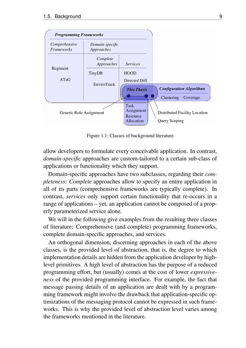
In this section, we place the three contributions of this thesis, summarizedabove, in the context of related literature. Although specific related workwill be discussed next to each contribution in the respective chapter, inthis section we attempt a more high-level view on classes of related litera-ture. Depending on the taken point of view, these may be associated withvarious research domains as shown in Figure 1.1.
On the one hand, generic role assignment provides a programmingframework for wireless sensor networks. We will discuss programmingframeworks in detail in Section 1.5.1. At the same time, it can be viewedas a highly parameterizable network configuration algorithm, for whichthe role assignment specification provides a succinct parameterization in-terface. While all three contributions share this dual view, we will arguethat the provided contributions are more generic than existing literatureon configuration algorithms in Section 1.5.2. Finally, as the assignmentof a role to a node usually implies assigning a certain task to the node (or,vice versa, allocating the node’s resources for a task), our contributionson role-based configuration are related to approaches for task assignmentand resource allocation, as we will describe in Sections 1.5.3 and 1.5.4.
1.5.1 Programming Frameworks
We subclass approaches that provide programming support for wirelesssensor networks using two attributes: The first is their comprehensive-ness. Comprehensive programming frameworks focus on replacing ex-isting low-level programming approaches. In this regard, their aim is to
1.5. Background 9
ComprehensiveFrameworks
ServicesCompleteApproaches
Domain-specific Approaches
Programming Frameworks
Configuration Algorithms
Regiment
ATaG
TinyDB
EnviroTrack
HOOD
Clustering Coverage
TaskAssignmentResourceAllocation
Directed Diff.
This Thesis
Distributed Facility LocationGeneric Role Assignment
Query Scoping
Figure 1.1: Classes of background literature
allow developers to formulate every conceivable application. In contrast,domain-specific approaches are custom-tailored to a certain sub-class ofapplications or functionality which they support.
Domain-specific approaches have two subclasses, regarding their com-pleteness: Complete approaches allow to specify an entire application inall of its parts (comprehensive frameworks are typically complete). Incontrast, services only support certain functionality that re-occurs in arange of applications – yet, an application cannot be composed of a prop-erly parameterized service alone.
We will in the following give examples from the resulting three classesof literature: Comprehensive (and complete) programming frameworks,complete domain-specific approaches, and services.
An orthogonal dimension, discerning approaches in each of the aboveclasses, is the provided level of abstraction, that is, the degree to whichimplementation details are hidden from the application developer by high-level primitives. A high level of abstraction has the purpose of a reducedprogramming effort, but (usually) comes at the cost of lower expressive-ness of the provided programming interface. For example, the fact thatmessage passing details of an application are dealt with by a program-ming framework might involve the drawback that application-specific op-timizations of the messaging protocol cannot be expressed in such frame-works. This is why the provided level of abstraction level varies amongthe frameworks mentioned in the literature.
10 Chapter 1. Introduction
Comprehensive Programming Frameworks
The focus of comprehensive programming frameworks is to replace ex-isting sensor network programming approaches, and, typically, allow de-velopers to implement every conceivable application using the providedframework.
The front-end of such programming frameworks are programming ab-stractions, which define the set of primitives that can be used by devel-opers to formulate the task at hand. The user program is then translated,either by a compiler or by adequate run-time support, into node-level in-structions that aim to implement the semantics of the program efficiently.
At the highest level of abstraction, so-called macroprogramming ap-proaches shield developers from the complexity of programming individ-ual nodes. Instead, developers issue high-level programs that specify thedesired global behavior of the application in terms of resources of the net-work. Typically, such programs make use of various high-level constructssuch as data structures managing sets of nodes, variables implicitly sharedamong nodes, and specifications of the global data flow required for theapplication, which, so the authors argue, can more effectively express thedesired application logic than node-level programs. These programs arethen translated into a set of commands for individual nodes.
Typical macroprogramming systems are Regiment [NW04, NMW07] –which uses functional programming constructs that operate over individ-ual events, over streams of events, and over groups of nodes that gener-ate them – and the Kairos [GGG05] system, which provides a procedu-ral interface for specifying global application behavior. Other examplesare ATaG [BPRL05], whose specification combines custom-implementedmodular tasks with a graph-based specification of the flow of informa-tion between tasks, and spatial programming [BIK+04] which allowsprogrammers to express the desired computation in terms of geospatialreferences to the resources of the network.
At lower levels of abstraction, programming frameworks typically pro-vide a greater expressiveness but come with increased programming com-plexity. In such frameworks, it is often required to program on the levelof individual nodes, for example, one must specify which data a nodeshould sample and which messages to send or receive. One such exam-ple is SensorWare [BS03], whose input are node-level scripts supportedby a script migration and replication middleware. A second example isFACTS [TWS06], in which developers specify data-processing rules con-
1.5. Background 11
sisting of trigger conditions (usually in terms of incoming data) and asso-ciated actions (a set of operations manipulating or sending data once therule fires).
On the lowest and most expressive abstraction level, several approachesprovide novel node-level programming paradigms [KR05], intermedi-ate languages [NAW05], or virtual machines [LC02] that improve overcertain deficiencies that are present in the most wide-spread node-leveloperating systems such as [TOS]. Such approaches may also serve ascompilation targets onto which compilers map more high-level abstrac-tions. Other examples, Impala [LSZM04], SOS [HKS+05], or Con-tiki [DGV04], provide “enhanced” operating systems integrating node-level programs with middleware support, e.g., for component manage-ment and code-deployment.
Complete Domain-specific Approaches
Domain-specific approaches, in turn, can be divided up in two subclasses(cf. Figure 1.1) . In the first class, complete approaches allow to specifyapplications in all their parts.
Perhaps the most wide-spread members of this class provide adatabase view on sensor networks and on the data they sample (e.g.,Cougar [BGS01] or TinyDB [MFHH03, MFHH05]). By means of adeclarative query interface, these systems support various classic datagathering applications by allowing users to subscribe to a desired streamof sensor data.
Complementary systems focus on supporting various other applicationclasses. For example, DSWare [LSS03] allows users to specify eventsthat should be detected by a network (such as a fire), IrisNet [GKK+03]adds functionality for managing data generated by sensor networks inter-connected by a wide-area backbone, and, finally, EnviroTrack [ABC+04]provides primitives for implementing applications that deal with trackingmoving real-world phenomena. Recently, EnviroTrack has been embed-ded into a more comprehensive programming framework called Enviro-Suite whose abstractions revolve around real-world entities observed bythe network [LAHS06].
Services
In contrast, a second subclass of domain-specific systems, which we referto as services, supports certain functionality that manifests itself in many
12 Chapter 1. Introduction
applications. While a wider range of applications may benefit from suchservices, these cannot be used to specify an application completely. Thisis the case even when a service is rather generic and exports a certain pro-gramming interface for specifying its behavior. Consequently, some partsof the application must either be implemented on the operating systemlevel or provided by complementary services.
Compared to the previous two classes, the benefit of employing ser-vices for developing wireless sensor network applications is twofold. Onthe one hand, composing an application from a choice of services allowsapplication developers to benefit from high-level abstractions for address-ing certain functionality (if the service’s abstraction semantics match thedeveloper’s intention well) but at the same time they are free to revert toany lower but more expressive level of abstraction for other domains offunctionality (e.g., implementing a novel localization protocol that is par-ticularly suitable in the application or a driver for a specific sensor board).That is, integrating services into an application (or, alternatively, into aprogramming framework) provides developers with increased flexibility,as applications can be programmed on a heterogeneous abstraction level,custom-tailored to an application’s needs.
Generic role assignment belongs to this class: It supports developerssolely with network configuration tasks. By means of role specifica-tions, developers may specify the desired network structure. The rest ofthe application is expected to be implemented by custom-made softwarecomponents. An event-based architecture provides the glue between therole assignment system and other application components executed on thenodes.
As a member of this class, generic role assignment co-exists with otherapproaches that provide services addressing various domains of func-tionality on various abstraction levels. For example, neighborhood man-agement services such as HOOD [WSBC04], but also [WM04, MP06,SFCB04], alleviate programmers from the details of message passing anddata sharing within certain local network neighborhoods. Each of theabove includes functionality to manage the membership in these neigh-borhoods, a functionality which is often referred to as scoping.
Such scoping is often provided as a distinct service, which can be imple-mented either topologically, e.g., by constraining neighborhoods to a cer-tain number of hops in the network communication graph or by providingcustom-implemented neighborhood definitions such as trees [WM04], orgenerically, e.g., based on conditions formulated in terms of various other
1.5. Background 13
node properties that define a node’s membership in a certain neighbor-hood [SFCB04, MP06]. The fact that the latter approaches use techniquesthat are similar to role assignment to evaluate a node’s membership in thescope (dual to the way role assignment evaluates the node’s membershipin the set of nodes which are assigned a certain role) implies that genericrole assignment can also be viewed as a scoping approach. Our queryscoping contribution (described in Chapter 4) provides a similar servicebut for a different class of applications which require that scoping deci-sions are performed before network nodes (in particular nodes outside ofthe computed scope) are involved in any communication or computation.
Other examples of this class are the TinyLime [CGG+05] middlewareproviding the notion of a transparent tuple space in which sensor data canbe stored. Similarly, geographic hash tables provide for in-network stor-age of gathered data [GEG+03]. The seminal Directed Diffusion [IGE00]system provides a content-based routing service allowing nodes to sub-scribe to arbitrary data provided by the network. A subscription, so-calledinterest, specifies the data that should be delivered at the node by meansof attribute value pairs.
Numerous other services exist in the literature supporting various func-tionality. We used the above services as examples, as they (like genericrole assignment) export programming abstractions which can be used toimplement a certain behavior of the service. These abstractions, from adifferent point of view, provide efficient and succinct interfaces for pa-rameterizing the execution of the provided service. The underlying im-plementation is a highly parameterizable configuration algorithm.
1.5.2 Configuration Algorithms
In contrast to our generic approaches, many algorithms address specificrole-based network configuration problems. We have mentioned clus-tering [Lub85, HCB00, KG02], data aggregation [BB03], and cover-age [XHE01, MKPS01, GZDG05].
Apart from role-based configuration, many other specialized configu-ration algorithms exist. Examples include channel assignment [Ram99](based on distributed graph coloring approaches) and topology control al-gorithms [WZ04, San05] (which regulate the transmit power used whencommunicating with neighbors).
Some of these algorithms provide interfaces to parameterize their exe-cution. These interfaces can differ in their expressiveness. For example,

14 Chapter 1. Introduction
[KG02] allows to set two parameters which determine the number of gate-way nodes which are used to join clusterheads into a connected topology.
Compared to existing role-based configuration algorithms, the threecontributions of this thesis provide more powerful parameterization in-terfaces which make them applicable to a wider range of configurationtasks. Making use of the provided interfaces, developers may install onealgorithm and afterwards rapidly re-configure the network’s behavior in avariety of ways by issuing new parameters to these algorithms.
Each contribution targets a different application domain and thereforeprovides a different parameterization interface. The generic role assign-ment framework, described in Chapter 2, extracts the parameters deter-mining algorithm execution from a given role assignment specification.The distributed facility location algorithm, described in Chapter 3, is per-haps the most specific configuration algorithm. Its parameterization isperformed by adequately chosen opening costs (assigned to nodes) andconnection costs (assigned to links). Finally, the query scoping system ofChapter 4 uses an annotated data model for parameterizing its execution.
1.5.3 Task Assignment
Last but not least, we would like to mention a couple of adjacent researchareas out of which some aspects are addressed by the contributions pro-vided in this thesis.
For example, we mentioned in the above that it is sometimes desirableto obtain a role assignment that minimizes the overall costs of communi-cation between nodes of different roles. Our distributed facility locationalgorithms, for instance, select a cost-optimal set of servers while takinginto account the cost of communication between clients and their closestserver. More generally, one might consider taking larger structures of de-pendencies between roles into account. For example, the placement ofdifferent aggregator roles should minimize total communication cost ofthe whole aggregation tree.
In the distributed systems field, this problem setting is known as taskassignment. The task assignment problem is motivated by the need todistribute a set of program modules (or computation tasks) to a set ofprocessors while minimizing the cost of communication between them.Our systems also assign modules to sensor nodes by means of the roleabstraction: The assignment of a role to the local node typically triggersthe execution of program modules previously associated with the role.

1.5. Background 15
Solving the task assignment problem for arbitrary communication de-pendencies between different modules is hard. An early approach [Sto77]described a set of centralized network-flow-based algorithms that solvedtask assignment in polynomial time for two processor nodes (proces-sors correspond to sensor nodes in our models). While flow-based tech-niques were extended to three processors, for four and more processorsthe problem was shown to be NP-hard [Bok87]. What proved to be easieris solving task assignment when communication dependencies betweendifferent modules have the form of a tree. Here, a centralized algo-rithm [Bok81] solves the task assignment problem based on finding short-est paths in a graph generated from the network communication graph andthe dependency graph between modules.
An example task assignment approach adapted for wireless sensor net-works is [BB03], which assigns a tree of query operators (generated froma declarative database query) to network nodes. The approach attempts tominimize data traffic between operators – and therefore provide for effi-cient query execution. It is based on a hill-climbing technique that, givenan initial placement of the operator tree, moves operators to neighboringnodes if these can perform the operator function more efficiently.
Similarly, the MagnetOS system [LRW+05], aims to assign the mod-ules of a global program to the nodes of a network graph. The approachevaluates various heuristics to place modules. Such heuristics include tomove a module to the neighbor with which it communicates most, or to amore suitable node based on a partial view of the network aggregated atthe local node.
1.5.4 Resource Allocation
The resource allocation problem [Lyn81] goes beyond selecting nodes forexecuting certain modules but allocates goods (such as sensor time on anode, node computation, or bandwidth) for a certain global task. Simi-larly, role assignment can be considered to allocate a node’s processingpower, sensors, and transceiver to a certain task implied by the role.
One example of a resource allocation approach [MPW05] for sensornetworks uses virtual-market oriented heuristics for this purpose build-ing on similar approaches for distributed systems [Cle96]. Here, nodesattempt certain actions (such as listen, sense, or send) each of which areassociated with a certain cost in terms of consumed energy – and a certainreward if the taken action was successful. Developers may parameterize

16 Chapter 1. Introduction
the reward for each action, which, as nodes aim to optimize their rewardbased previous actions, provide high-level levers for controlling the net-work’s behavior.
Summing up, both, task assignment and resource allocation approachesexplore functionality complementing the role-based configuration ap-proaches considered in this thesis. Task assignment additionally opti-mizes the configuration based on the communication involved betweennodes with different roles. Resource allocation expands the consideredfunctionality in the time dimension, as it allows to assign node resourcesto different tasks over time.
While such functionality is intriguing, both problem classes are verydemanding in terms of computing complexity. For example, the aboveapproaches for wireless sensor networks [MPW05, BB03] both involveresource-intensive trial phases in which improvements of the current so-lution are explored. In [BB03], all neighbors of an operator simulate theoperator’s function (including the involved communication) in order toevaluate the benefit of a possible re-location of the operator. In [MPW05],nodes “attempt” certain actions at random in order to evaluate whether theexecution of such actions is beneficial.
1.6 Summary
In this chapter, we have provided an introduction to the three contributionsof this thesis and overviewed the corresponding background literature.
In summary, we claim that role-based network configuration is an im-portant challenge which re-appears in heterogeneous wireless sensor net-work applications and network models. For the domain at hand, suitableconfiguration algorithms must be found. This thesis therefore provides ef-fective system support for such role-based configuration, first in a genericapproach and then for two subclasses of problems. In its contributions,this work sheds light on a range of configuration approaches, each con-sisting of a parameterization interface and an underlying implementation.In this, the presented thesis examines three different points in the trade-off between, on the one hand, the simplicity and the expressiveness ofthe configuration interface and, on the other hand, the performance andthe efficiency of the underlying implementation. Taken together, the pro-vided configuration support represents a step forward on the path towardsplug and play sensor network systems. Such improved usability, often

1.7. Outline 17
presumed a key prerequisite to wide-spread usage of wireless sensor net-works, would finally enable the economies of scale commonly associatedwith the wireless sensor network vision.
Parts of this thesis have been published in proceedings of internationalconferences and workshops, most notably in [RFMB04, FR05, FR06,FR07, FRNK06, FBRK07].
1.7 Outline
This thesis is structured as follows. We first present the role assignmentabstraction, its implementation, and its extensions in Chapter 2. In thefollowing two chapters, we then address two subclasses of role assign-ment problems. In Chapter 3, we describe an approach concerned withcomputing near-optimal clustering decisions in a distributed manner. InChapter 4, we discuss an approach for offline query scoping in a large-scale mobile-phone-based sensor network.
A set of aspects will re-appear in each of these chapters: The interfaceof the configuration service, examples for its use, the algorithms that con-stitute the implementation of this interface, and an evaluation regardingthe efficiency and feasibility of the approach.
Based on the contributions detailed in Chapters 2, 3 and 4, we extractcommon guidelines for the development of future programming supportfor wireless sensor networks and conclude our work in Chapter 5.

18 Chapter 1. Introduction
2 Generic Role Assignment
In this chapter, we present a programming framework called generic roleassignment that allows users to define a list of roles which will be assignedto sensor nodes if certain conditions are met. Above, we mentioned thatseveral classic network configuration problems can be viewed as instancesof generic role assignment. As an introduction to this chapter we sketchthree role assignment problems and list the involved roles together withpossible conditions for their assignment.Coverage. A certain area is said to be covered if every physical spotfalls within the observation range of at least one sensor node. In densenetworks, each physical spot may be covered by many equivalent nodes.The lifetime of the sensor network can be extended by turning off theseredundant nodes and by switching them on again when previously activenodes run out of battery power [XHE01]. Essentially, this requires properassignment of the roles ON and OFF to sensor nodes.Clustering. Clustering is a common technique to improve the efficiencyof data delivery (e.g., flooding, routing) [KG02]. With clustering, oneof the three roles CLUSTERHEAD, GATEWAY, SLAVE is assigned toeach node. A clusterhead acts as a hub for slaves in its neighborhood suchthat slaves directly communicate with their clusterhead only. Gatewaysare slaves of more than one cluster and interconnect multiple clusters byforwarding messages between them.In-network Aggregation. Due to the scarcity of energy and the highenergy cost of wireless communication, reducing data communication isan important design goal in sensor networks. One common form of datareduction is in-network data aggregation, where certain nodes in the net-work aggregate sensory data from many sources [IGE00]. For this, sen-sor nodes must be assigned the roles SOURCE (generate sensory data),AGGREGATOR (aggregate data), and SINK (consume aggregated data)roles. In order to achieve a significant network traffic reduction, aggrega-tor nodes should be located close to the data sources they aggregate.
While a number of specialized algorithms for these problems have beendeveloped, these are typically hard to adapt to different applications,
20 Chapter 2. Generic Role Assignment
where varying criteria for assigning the above roles may have to be ap-plied. Driven by these observations, our aim is to provide a generic roleassignment service that is applicable to a wide variety of role assignmentproblems. We first give an overview of the various components involvedin generic role assignment. These components will be described in detailin the remainder of this chapter.
2.1 Overview
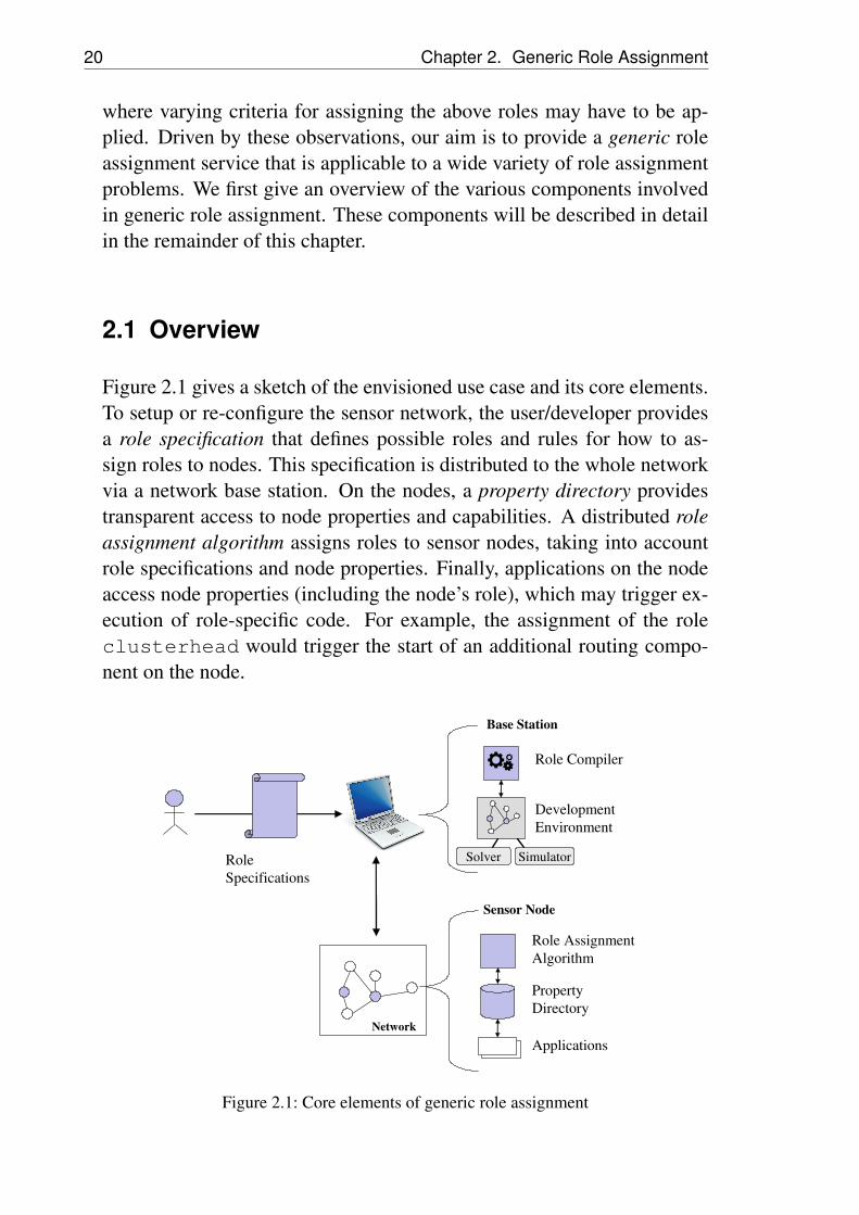
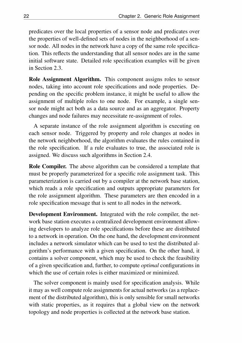
Figure 2.1 gives a sketch of the envisioned use case and its core elements.To setup or re-configure the sensor network, the user/developer providesa role specification that defines possible roles and rules for how to as-sign roles to nodes. This specification is distributed to the whole networkvia a network base station. On the nodes, a property directory providestransparent access to node properties and capabilities. A distributed roleassignment algorithm assigns roles to sensor nodes, taking into accountrole specifications and node properties. Finally, applications on the nodeaccess node properties (including the node’s role), which may trigger ex-ecution of role-specific code. For example, the assignment of the roleclusterhead would trigger the start of an additional routing compo-nent on the node.
Role
Specifications
Property
Directory
Role Assignment
Algorithm
Base Station
Applications
Network
Sensor Node
Role Compiler
Development
Environment
Solver Simulator
Figure 2.1: Core elements of generic role assignment
2.1. Overview 21
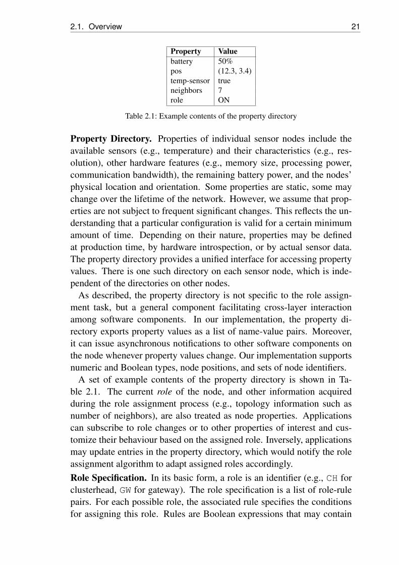
Property Valuebattery 50%pos (12.3, 3.4)temp-sensor trueneighbors 7role ON
Table 2.1: Example contents of the property directory
Property Directory. Properties of individual sensor nodes include theavailable sensors (e.g., temperature) and their characteristics (e.g., res-olution), other hardware features (e.g., memory size, processing power,communication bandwidth), the remaining battery power, and the nodes’physical location and orientation. Some properties are static, some maychange over the lifetime of the network. However, we assume that prop-erties are not subject to frequent significant changes. This reflects the un-derstanding that a particular configuration is valid for a certain minimumamount of time. Depending on their nature, properties may be definedat production time, by hardware introspection, or by actual sensor data.The property directory provides a unified interface for accessing propertyvalues. There is one such directory on each sensor node, which is inde-pendent of the directories on other nodes.
As described, the property directory is not specific to the role assign-ment task, but a general component facilitating cross-layer interactionamong software components. In our implementation, the property di-rectory exports property values as a list of name-value pairs. Moreover,it can issue asynchronous notifications to other software components onthe node whenever property values change. Our implementation supportsnumeric and Boolean types, node positions, and sets of node identifiers.
A set of example contents of the property directory is shown in Ta-ble 2.1. The current role of the node, and other information acquiredduring the role assignment process (e.g., topology information such asnumber of neighbors), are also treated as node properties. Applicationscan subscribe to role changes or to other properties of interest and cus-tomize their behaviour based on the assigned role. Inversely, applicationsmay update entries in the property directory, which would notify the roleassignment algorithm to adapt assigned roles accordingly.Role Specification. In its basic form, a role is an identifier (e.g., CH forclusterhead, GW for gateway). The role specification is a list of role-rulepairs. For each possible role, the associated rule specifies the conditionsfor assigning this role. Rules are Boolean expressions that may contain
22 Chapter 2. Generic Role Assignment
predicates over the local properties of a sensor node and predicates overthe properties of well-defined sets of nodes in the neighborhood of a sen-sor node. All nodes in the network have a copy of the same role specifica-tion. This reflects the understanding that all sensor nodes are in the sameinitial software state. Detailed role specification examples will be givenin Section 2.3.
Role Assignment Algorithm. This component assigns roles to sensornodes, taking into account role specifications and node properties. De-pending on the specific problem instance, it might be useful to allow theassignment of multiple roles to one node. For example, a single sen-sor node might act both as a data source and as an aggregator. Propertychanges and node failures may necessitate re-assignment of roles.
A separate instance of the role assignment algorithm is executing oneach sensor node. Triggered by property and role changes at nodes inthe network neighborhood, the algorithm evaluates the rules contained inthe role specification. If a rule evaluates to true, the associated role isassigned. We discuss such algorithms in Section 2.4.
Role Compiler. The above algorithm can be considered a template thatmust be properly parameterized for a specific role assignment task. Thisparameterization is carried out by a compiler at the network base station,which reads a role specification and outputs appropriate parameters forthe role assignment algorithm. These parameters are then encoded in arole specification message that is sent to all nodes in the network.
Development Environment. Integrated with the role compiler, the net-work base station executes a centralized development environment allow-ing developers to analyze role specifications before these are distributedto a network in operation. On the one hand, the development environmentincludes a network simulator which can be used to test the distributed al-gorithm’s performance with a given specification. On the other hand, itcontains a solver component, which may be used to check the feasibilityof a given specification and, further, to compute optimal configurations inwhich the use of certain roles is either maximized or minimized.
The solver component is mainly used for specification analysis. Whileit may as well compute role assignments for actual networks (as a replace-ment of the distributed algorithm), this is only sensible for small networkswith static properties, as it requires that a global view on the networktopology and node properties is collected at the network base station.
2.2. Related Work 23
Basic Services. A number of basic services such as node localization,neighbor/topology discovery, or time synchronization may add valuableinformation to the property directory. The availability of such servicescould also be a node property. These services are decoupled from the restof the system through the property directory.
The remainder of this chapter is organized as follows. After survey-ing related background literature in Section 2.2, we introduce a languagefor specifying roles in Section 2.3. Section 2.4 presents distributed algo-rithms for role assignment. The development environment and the imple-mentation of the distributed algorithms is discussed in Section 2.5. Weevaluate the efficiency of these algorithms quantitatively in Section 2.6and qualitatively, by comparing the semantics of our role assignment sys-tem to specialized role assignment implementations from the literature, inSection 2.7. Finally, we present the role assignment solver in Section 2.8and provide an outlook to an extended role specification syntax in Sec-tion 2.9.
2.2 Related Work
Self-configuration in ad hoc and sensor networks has been an active re-search topic in the recent past. Various other approaches for solving spe-cific self-configuration problems have been devised. Examples includecoverage [SP01]; aggregator placement [BB03]; clustering, routing andaddressing [KSG03, SAGP00, SK00]. [KSG03] uses a fixed set of rolesto build a network-wide backbone infrastructure. However, none of theseapproaches are generic frameworks that support the assignment of user-defined roles in an application-specific manner.
The concept of role assignment has been mentioned in various researchprojects related to wireless sensor networks. In [HMCP04], a middle-ware called MiLAN is outlined that controls the allocation of functionsto sensor nodes in order to meet certain quality-of-service requirementsspecified by the user. In [MLM+05], a cross-layer framework called Tiny-Cubus is presented that uses the notion of roles to implement efficientcode deployment. In [UWMG05], a high-level programming approachfor sensor networks is presented, where a high-level task specification iscompiled into a set of node-level programs that must be properly allocatedto sensor nodes taking into account the node capabilities.
Moreover, neighborhood programming abstractions [WM04,WSBC04] have been proposed, where network neighbors can eas-
24 Chapter 2. Generic Role Assignment
ily share variables among each other. These abstractions pose aninteresting opportunity for implementing our role assignment approach.In particular, each node in the network could set up a “sharing region” inorder to exchange property values among nodes.
Inspired by cellular cooperation in biological organisms, AmorphousComputing [AAC+00] explores ways to program smart matter – verydensely deployed collections of indistinguishable smart particles. In con-trast, our approach is based on the observation that sensor nodes maysignificantly differ in their properties, may rely on a number of basic ser-vices (e.g., localization), and are less densely deployed. Also, we focuson the configuration of sensor networks, the actual “programming” (i.e.,distributed data processing etc.) is not part of our work, although rolesand other property values derived during role assignment may providevaluable input.
Our scheme for role assignment is somewhat similar to cellular au-tomata [Wol94], where the state of a particle in a regular arrangementis completely defined by the previous values of a neighborhood of parti-cles around it. Note that a classification of a subclass of cellular automatain [Wol94] indicates that a large group of automata converges to well-defined states. Major differences of our approach are that state updatesare not synchronous, sensor nodes are not in a regular arrangement, andsensor nodes differ in their properties.
The role assignment solver complements the distributed role assign-ment algorithms by using integer linear programs (ILPs) to compute exactsolutions to generic role assignment problems. ILPs have been appliedto network configuration problems in various settings. In [BC02], theauthors derive upper bounds on the lifetime of data-gathering networksby computing optimal configurations consisting of the roles sensor, re-lay, and aggregator. Moreover, integer program formulations have beenused as a starting point for developing distributed approximation algo-rithms which solve problems that are related to our specifications, mostprominently the minimum dominating set [KW03] and the facility loca-tion problem [MW05]. The latter approach [MW05] addresses an impor-tant subset of role assignment problems and will be discussed in detailwhen we address these problems in Chapter 3. Compared to these ap-proaches, the role assignment solver provides a generic framework fortranslating any role assignment problem into an ILP.

2.3. Role Specifications 25
2.3 Role Specifications
In this section we introduce the notation for role specifications. We firstshow how this approach can be used for a number of applications, laterwe will review the essential specification components in more detail.
2.3.1 Application Examples
Let us revise the examples sketched in the introduction into more formalspecifications. Note that these role specifications will typically result inapproximate solutions of the respective configuration problems.Coverage. As mentioned earlier, nodes must be assigned ON and OFFroles. Requirements for the assignment of these roles are that the area ofinterest is covered by the sensors of ON nodes, and that ON nodes have suf-ficient remaining battery power. Assuming one is interested in coveragewith temperature readings, one possible formulation could be:
1 ON :: {2 temp-sensor == true &&3 battery >= threshold &&4 count(2 hops) {5 role == ON &&6 dist(super.pos, pos) <= sensing-range7 } <= 1 }8 OFF :: else
The rule in lines 1-7 specifies the conditions for a node to have ON status:it must have a temperature sensor and enough battery power (lines 2 and3). As a third condition, we require that at most one other ON node shouldexist within this node’s sensing range. This is specified by the countoperator in line 4. It expects a hop-range as its first parameter and re-turns the number of nodes within this range for which the expression incurly braces evaluates to true. Here we request to evaluate nodes within2 network hops. Note that the used property names (e.g., role in line 5,pos in line 6) in the nested expression refer to properties of the specifiedneighboring nodes. To access properties of the local node instead, theprefix super is used (e.g., super.pos in line 6). The dist operatorused in line 6 returns the metric distance between two positions. In theexample, it specifies that only nodes located within this node’s sensingrange should be counted.
In other settings it would be useful to retain state on network neighborsinstead of just counting them. Clustering is such an example.

26 Chapter 2. Generic Role Assignment
Clustering. A clustering approach needs to define assignment rules forclusterhead (CH), gateway (GW) and SLAVE roles. The assignment ofthese roles depends on a variety of parameters. Clusterheads should bemore powerful devices (in terms of processing, memory, communication,and energy supply), because they act as hubs for many slaves. This maybe easily formulated in terms of the property directory and is neglectedhere. For a role specification, consider the following basic scheme:
1 CH :: {2 count(1 hop) {3 role == CH4 } == 0 }5 GW :: {6 clusterheads == retrieve(1 hop, 2) {7 role == CH8 } &&9 count(2 hops) {
10 role == GW &&11 clusterheads == super.clusterheads12 } == 0 }13 SLAVE :: else
A node that does not have any clusterhead among its neighbors declaresitself clusterhead (CH, lines 1-4).
Nodes should be assigned the role gateway (GW) if they are neighborsto at least two clusterheads but are not aware of any other gateway nodesinterconnecting the same two clusterheads.
To achieve this, we introduce the retrieve operator (line 6), whichis similar to count, but returns a set of node identifiers instead ofonly counting the nodes. In this example, the retrieve operator is usedto identify clusterheads in the 1-hop neighborhood of the node and tobind them to the local property clusterheads in line 6 (similar tobinding of variables in declarative programming languages). Using theclusterheads property, we require in lines 9-12 that within 2 hops noother gateways should interconnect the same set of clusterheads.
The second parameter to retrieve in line 6 requests any two match-ing nodes. If not enough matching nodes exist, the retrieve expressionevaluates to false. In this case, the GW role is not assigned, the propertyclusterheads remains undefined, and the evaluation of lines 9-12 canbe omitted.In-network Aggregation. Similar rules can be designed for an exemplaryapplication requiring in-network aggregation.

2.3. Role Specifications 27
1 AGG2 :: { analogous to AGG1 }2 AGG1 :: {3 count(2 hops) {4 role == SOURCE &&5 dist(pos, sink-pos) >6 dist(super.pos, sink-pos)7 } >= 2 &&8 count(2 hops) {9 role == AGG1
10 } == 0 }11 SOURCE :: { temp-sensor == true }
In this example, sensor nodes equipped with temperature sensors act asdata sources (line 11). A single sink node with known position sink-posconsumes aggregated data. Aggregator nodes (AGG1) should be placed inthe close neighborhood of many sources (line 4) compared to which theaggregator is closer to the sink (lines 5-6) because data flows from sourcesto the sink. We furthermore require that no other nodes with role AGG1should exist within two hops.
Note that we used a second role AGG2 for aggregators of higher levelwhich aggregate information from nodes with role AGG1 instead ofsources. AGG2 nodes should be similarly placed between the AGG1 nodesand the sink and no other AGG2 nodes should exist in their 2-hop neigh-borhood.
2.3.2 Syntax and Semantics
Let us review the specification techniques introduced in the examples. Arole specification consists of a list of roles and associated conditions in-volving the values of local properties of a sensor node or the propertiesof well-defined sets of nodes in the neighborhood of the node. The con-ditions for a role k are determined by an associated role predicate ck. Weassume ck has been preprocessed by the role compiler and rearranged intoits disjunctive normal form:
ck = (ck11∧·· ·∧ ck
1n1)∨ (ck
21∧·· ·∧ ck2n2
)∨ . . . (2.1)
Three types of atomic predicates cki j are supported:
Simple predicates are essentially Boolean expressions formulated interms of properties and constants, possibly involving basic arith-metic operations.
Count predicates of the form
28 Chapter 2. Generic Role Assignment
count(scope) { pred } rel const
can be used to count nodes that match a nested predicate predwithin a given number of hops scope around the current node andcompare the result to a constant expression const using a givenrelation rel.
Retrieve predicates are similar, these have the form
p == retrieve(scope,size) { pred }
and can be used to bind the identities of a set of nodes matchingpred to a local property variable p. A parameter size specifiesthat at least size matching nodes must exist, otherwise the predi-cate evaluates to false. After evaluation, p contains the identifiers ofthe matching nodes and can be used as a local property.
Within count and retrieve operators, the nested predicate pred spec-ifies the conditions under which a remote node is counted or retrieved,respectively. These conditions are arranged in a disjunctive normal formin which, essentially, only simple predicates are allowed. Because theproperties used in pred generally reference property values of remotenodes, it is furthermore possible to pre-pend super to property names toreference properties of the current node instead.
As mentioned earlier, the property directory supports numeric andBoolean types, node positions, sets of node identifiers, and the enumera-tion role. When comparing node property values, equality is supportedfor all properties, while the usual ordering relations (such as <, ≤ etc.)are additionally available for all numeric properties.
Note that because retrieve predicates bind local properties which canbe referenced by other count and retrieve statements, the former mustbe evaluated before predicates referencing the bound value. Moreover,the specification must not contain circular dependencies between any tworetrieve statements that are part of the conditions of any role. This ischecked by a compiler before sending the specification to the nodes. InSection 2.4, we describe distributed algorithms that can be used to imple-ment the semantics described above.
The presented specification language obviously cannot capture all con-ceivable role assignment problems (see also Section 2.7 on this issue).However, from our experience it can be used to implement practical ap-proximations of many configuration tasks. Moreover, our approach can

2.3. Role Specifications 29
be extended in two ways to be more powerful: Firstly, custom predicates(such as the dist operator mentioned earlier) can be implemented by theprogrammer to support complex role assignment tasks. Secondly, appli-cations may subscribe to certain role changes and changes of other prop-erties. When notified of such a change, the application may perform anycomputations that cannot be expressed directly with the role specificationlanguage. In addition, the application may set values in the property direc-tory, triggering the role assignment algorithm to revise role assignmentsto take into account the modified properties.
Generally, the role assignment abstraction enables the programmer toaddress configuration problems based on rather stable network proper-ties (where there is a limit on the frequency of changes of properties onwhich the configuration decisions are based). In order to perform con-figuration, any algorithm that implements role assignment will have toreach consensus on the current state of the network within local networkneighborhoods around each node.
Crucial for the locality of any role assignment algorithm is the givenscope that is used in count and retrieve statements because it governs thedegree of interdependence between nodes. We therefore define the maxi-mum scope of a specification:
Maximum Scope. The maximum scope of a given specification is thehighest hop-number used as a scope for count and retrieve statements.
Similarly we introduce a term for the set of nodes that can influence therole selection of a given node:
Critical Area. The critical area of a node u is the set of nodes v with
0 < d(u,v)≤ maximum scope
where d(u,v) is the hop-length of the shortest path between u and v.
Next to the examples of Section 2.3.1, a range of basic building blocksfor network configuration can be specified using the presented role speci-fication language. For example, a tree rooted at the sink is easy to specifyusing adequately defined CHILD roles that set a node property parent.Moreover, it is possible to formulate NP-hard configuration problems us-ing role assignment specifications, which implies that a role assignmentcannot be computed within a guaranteed polynomial runtime. We will listsuch role specification examples in Section 2.9.

30 Chapter 2. Generic Role Assignment
In the following, we describe a set of practical heuristics for role as-signment which are efficient in the average case. The overhead of thepresented algorithms will later be tested with a range of typical role spec-ifications and network topologies in Section 2.6.
2.4 Distributed Role Assignment Algorithms
We motivated generic role assignment and sketched a possible distributedalgorithm that could be used to implement role assignment in a positionpaper [RFMB04]. This algorithm is based on a fixpoint iteration, whereeach node would repeatedly fetch the current values of all relevant remoteproperties in order to evaluate the role predicates, eventually deciding ona (preliminary) role for itself. These evaluation cycles would have to beproperly sequentialized among neighboring nodes in order to ensure con-sistent role assignments. Assuming that there is a fixpoint configuration,each node would end up with a role that does not change in subsequentevaluation cycles.
While this approach works in principle, it turns out that the overheadfor locking and unlocking neighbors for sequentialization is prohibitivelyhigh. Therefore, we have examined more efficient algorithms that proac-tively distribute property values to neighbors. This is based on the obser-vation that a node can decide which of its property values are relevant towhat neighbors, because each node uses the same role specification.
This proactive approach [FR05] eliminates much of the overhead for“locking” nodes and concurrently introduces some redundancy that makesit more robust in the face of message loss. We present the basic algorithmbelow. Later in Section 2.4.7 we introduce two probabilistic initializationschemes that make it more efficient.
It must be emphasized that the algorithms are heuristics which may re-sult in temporary inconsistencies due to the lack of sequentialization. Wewill employ randomized delays in order to avoid such inconsistencies. Ifa temporary inconsistency should occur, it will be removed in subsequentevaluations at one of the affected nodes.
The algorithms operate on a given role specification that needs to be dis-tributed to the nodes. Role specifications are encoded into byte-optimizedmessages at the sink using a syntax tree that is constructed from thegiven specification. Note that we do not focus on the (reliable) distri-bution of the role specification. While we have implemented a flooding-based approach, several well-studied protocols for code distribution ex-
2.4. Distributed Role Assignment Algorithms 31
ist [LPCS04]. In some contexts, the specification may also be loaded intothe node offline before deployment.
2.4.1 Overview
The basic algorithm is built around local cache tables maintained at eachnode, which contain a collection of (local and remote) properties that arerelevant for role assignment. Eventually, the node will refer to its cachetable to assign its own role, based on the information it has learned aboutits neighbors up to that time. We will refer to this as local rule evaluationas the node does not involve any additional remote data apart from its owncache.
In the upcoming subsections we will discuss how to initialize the node’scache table after the specification is received, how to propagate nodeproperties that have changed, how to perform the above-mentioned localrule evaluation, how to adapt to changing network properties, and finally,how to detect termination of the algorithm.
2.4.2 Initialization
The initialization of the local cache table is performed upon receiving anew role specification. As all nodes share the same specification, theywill essentially setup their tables in the same way.
In a first step, the node extracts the set of relevant properties from thespecification. Further, the node uses the specification to infer the distance(in hops) over which each property needs to be propagated at most, whichwe will refer to as the property’s max value. Such max values are com-puted from the scope of all count and retrieve operators within which therespective properties occur. Note that the node’s role is also a property forwhich a max value can be computed.
If a property is only used in (local) simple predicates, its max value is0 and the property will never be propagated to other nodes. Note that theinformation on property max values is constant for a given specificationand their maximum corresponds to the specification’s maximum scope.All these values are therefore pre-computed at the network base stationand included in the specification message that is injected into the network.
Using the above information, a given node A initializes its cache tableas shown in Figure 2.2. To illustrate the algorithm, we use a simplifiedcoverage specification – as depicted – where we assume that the node’s

32 Chapter 2. Generic Role Assignment
sensing range is equal to its transmission range and we specify that notwo neighbors are allowed to be ON concurrently.
1
1
1
Seq.No
0
0
0
Dist
1
0
0
Max
trueundefinedroleA
true100%batteryA
truetruetemp-sensorA
DirtyValueKeySource
1
1
1
Seq.No
0
0
0
Dist
1
0
0
Max
trueundefinedroleA
true100%batteryA
truetruetemp-sensorA
DirtyValueKeySource
Cache table of node A
ON :: {temp-sensor == true &&
battery >= 10% &&
count(1) {
role == ON} == 0 }
OFF :: ELSE
Specification
A
B C
Figure 2.2: Node A after initialization
The table is initialized with a row for each property used in the specifi-cation. Each row contains a field denoting the source node (which is A inthis case as information stems from A’s local properties), the property key,and its current value. Furthermore, a dist field denotes the hop-distancebetween the source node and A. At initialization this value is always 0because all information is local. The table also shows the max values de-scribed earlier which indicate how far the properties must be propagated.
Each row also contains a sequence number, which every node maintainsfor its local entries. It is initialized with 1 and increased every time a localproperty (with dist = 0) is updated. Finally, a dirty bit specifies whetherthis information was already propagated to neighbors (false) or not (true).Initially, this value is true.
The cache table – initialized with local properties as described here –contains redundant information that is already present in the property di-rectory. When optimizing for memory, these entries could be generatedjust-in-time from the local property directory instead. Similarly, the maxvalues could be stored only once for each property and dist values oncefor each node.
Once the cache table has been initialized, a node will schedule the exe-cution of three procedures that we will describe in the following subsec-tions (note that all random delays are uniformly distributed in the givenintervals).
2.4. Distributed Role Assignment Algorithms 33
Property Propagation after a random delay tprop ∼ (0,Tprop). The de-lay helps aggregating newly arriving information into a single mes-sage and at the same time spreads traffic over a longer time interval.See Section 2.4.3 for details.
Local Rule Evaluation is scheduled after an initial delay tinit. This de-lay is chosen to allow for adequate property propagation from allnodes in the current node’s critical area. It is computed from themaximum scope s using an additional random offset teval ∼ (0,Teval)to reduce the chance of simultaneous role evaluations:
tinit = sTprop + teval
Failure Detection at regular intervals Theartbeat.
2.4.3 Property Propagation
To transmit properties to its neighbors, a node creates an update message,essentially containing a list of cache table rows.
The message is composed from all rows with dirty = true and dist <
max. Entries with dist = max have reached their maximal scope and neednot be propagated any further (e.g., the local properties battery and temp-sensor in the coverage example). Essentially, the message contains a copyof these rows with the dist field increased by 1 and max and dirty fieldsleft out (dirty is true anyway and max values can be derived from thespecification). Furthermore, the node resets all dirty bits of its table tofalse. The resulting update message is broadcast to all neighbors. Notethat property keys can be efficiently encoded as an integer index, becauseall nodes use the same specification.
The receivers of such update messages enter the contained informationinto their local tables. If entries of the incoming message and the localtable refer to the same property of the same source node, the informationwith the larger sequence number is retained (note that sequence numbersare increased by the source node only, while other nodes forward themunmodified). If the information has taken a shorter path (source and se-quence number are the same, but dist field is smaller) the dist field is setto the smaller value.
On the first incoming update message, receivers schedule
Property Propagation after a random delay tprop ∼ (0,Tprop) in orderto forward new information with dist < max.

34 Chapter 2. Generic Role Assignment
Local Rule Evaluation after a random delay teval ∼ (0,Teval). Gener-ally, Teval is chosen to be larger than Tprop, see Section 2.4.4 for de-tails.
The property propagation delay tprop fulfills two functions at different lay-ers: Firstly, it is used to smooth out traffic bursts that would occur aftera property change that is forwarded over multiple hops. When using acontention-based MAC layer, this would additionally reduce collisions,as transmit attempts are spread over a longer period of time. Secondly, itreduces the number of update messages by collecting many “dirty” tablerows into a single message as shown in Figure 2.3.
Update msgs.
Propagation Local RuleEvaluation
tprop
teval
SummaryUpd.Msg.
Role Change Upd. Message
time
Figure 2.3: Property propagation and local rule evaluation
Our propagation procedure adds some redundancy when information isforwarded over multiple hops because one bit of information is typicallyforwarded over multiple paths. Yet this redundancy adds significantly tothe robustness of the algorithm in face of packet loss. We will examinerobustness in Section 2.6.
When the algorithm is used with low-duty-cycle MAC layers, one mustensure that the symmetry-breaking nature of the randomized timers is pre-served. This can be achieved either by making active periods sufficientlylong or by suspending algorithm timers in sleep periods (and thus stretchthe algorithm execution time). What is essential is that the MAC layerdoes not synchronize property propagation to such an extent that it forcesneighboring nodes to propagate past role changes simultaneously.
In our example from Figure 2.2, assume node A has recently updatedits role property to ON and thus also increased the row’s sequence num-ber. In A’s table, the only row with dist < max and dirty = true is therole property. A therefore broadcasts an update message to its neighborscontaining its role property entry only. Assume that, similarly, node Chas sent an update message, after it had picked the role OFF. Node B’scache table, after receiving update messages from A and C, is shown in
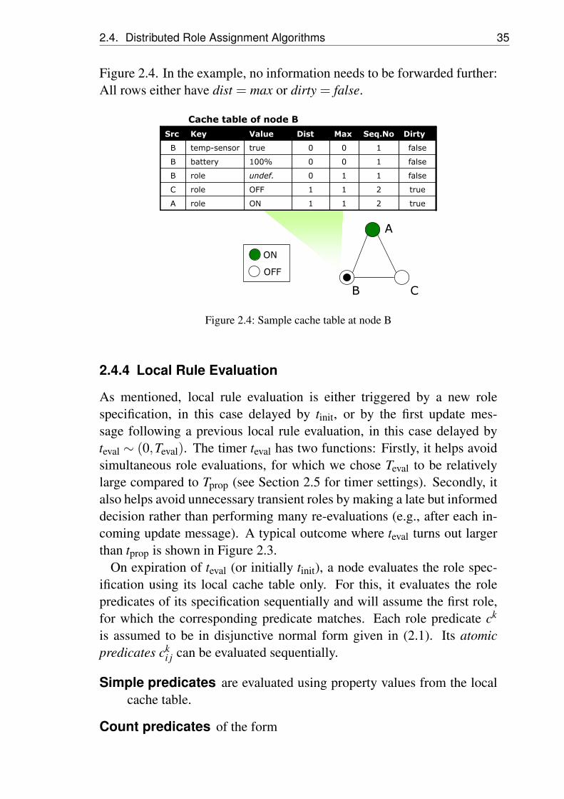
2.4. Distributed Role Assignment Algorithms 35
Figure 2.4. In the example, no information needs to be forwarded further:All rows either have dist = max or dirty = false.
true211ONroleA
true211OFFroleC
false110undef.roleB
1
1
Seq.No
0
0
Dist
0
0
Max
false100%batteryB
falsetruetemp-sensorB
DirtyValueKeySrc
true211ONroleA
true211OFFroleC
false110undef.roleB
1
1
Seq.No
0
0
Dist
0
0
Max
false100%batteryB
falsetruetemp-sensorB
DirtyValueKeySrc
Cache table of node B
A
B C
ON
OFF
Figure 2.4: Sample cache table at node B
2.4.4 Local Rule Evaluation
As mentioned, local rule evaluation is either triggered by a new rolespecification, in this case delayed by tinit, or by the first update mes-sage following a previous local rule evaluation, in this case delayed byteval ∼ (0,Teval). The timer teval has two functions: Firstly, it helps avoidsimultaneous role evaluations, for which we chose Teval to be relativelylarge compared to Tprop (see Section 2.5 for timer settings). Secondly, italso helps avoid unnecessary transient roles by making a late but informeddecision rather than performing many re-evaluations (e.g., after each in-coming update message). A typical outcome where teval turns out largerthan tprop is shown in Figure 2.3.
On expiration of teval (or initially tinit), a node evaluates the role spec-ification using its local cache table only. For this, it evaluates the rolepredicates of its specification sequentially and will assume the first role,for which the corresponding predicate matches. Each role predicate ck
is assumed to be in disjunctive normal form given in (2.1). Its atomicpredicates ck
i j can be evaluated sequentially.
Simple predicates are evaluated using property values from the localcache table.
Count predicates of the form

36 Chapter 2. Generic Role Assignment
count(scope) { pred } rel const
consider cache table rows with 1≤ dist ≤ scope. The nested pred-icate pred is then applied to the source nodes of all these rows. Thenumber of matching nodes is then compared to const using thegiven relation rel.
Retrieve predicates of the form
p == retrieve(scope,size) { pred }
are evaluated similarly. However, instead of only counting matchingnodes, a set S of matching nodes is computed. Note that a retrievestatement c binds p only while evaluating its enclosing conjunctionck
x = (c1∧·· ·∧cnx). If |S| < size, ckx evaluates to false. Otherwise,
the remainder of ckx is evaluated for all p ⊂ S with |p| = size until
the enclosing predicate ckx becomes true. If no such p exists, the
evaluation of ckx returns false.
If the node’s role has changed, property propagation is triggered withoutdelay.
In our example, node B performs local rule evaluation. B’s cache tableis shown in Figure 2.4. In the given example, B first checks the conditionsfor ON. Assuming that the node is equipped with a temperature sensor anda full battery, the first two conditions of the coverage specification eval-uate to true. Evaluating the count statement requires counting table rowswith property role and dist = 1. As the result of the count expression is 1,the predicate for role ON does not match. Node B continues by checkingthe conditions for OFF. As the “else” statement imposes no constraints,node B is assigned the role OFF.
2.4.5 Property and Network Dynamics
So far, we have described role assignment in a static network. In thissection, we consider the effects of changes in the network on a computedconfiguration. For this, we distinguish three classes of changes.
The first class are property changes, e.g., the battery level has changed.The property directory is configured to notify the role assignment systemof such changes. If a change occurred, the node updates the cache tableand re-examines its chosen role via the local rule evaluation procedure.

2.4. Distributed Role Assignment Algorithms 37
Only if the changed property value affects other (local or remote) proper-ties by changing the evaluation result of a predicate in the specification,an update message is composed and broadcast to all neighbors. Note thatthe number of update messages generated through property changes islimited by the minimal interval Tmin between two update messages thatare induced by property changes. The programmer may also specify atolerance interval ∆p for a property p, such that re-configuration is onlytriggered if p’s value changes by more than ∆p.
A second class of changes is when nodes join the network. For example,it is imaginable that additional nodes are deployed into a given area. Whensuch a new node overhears any protocol message, it first requests a copy ofthe role specification from its network neighbors. After it received a reply,it uses the specification to initialize as described earlier and broadcast anupdate message to inform neighbors of its relevant properties.
The third class are node failures. To detect such failures, nodes sendheartbeats every Theartbeat. A heartbeat is essentially an update message,containing the key of the property that needs to be propagated farthest inthe specification (e.g., the role property in our examples) with an emptyproperty value. The sequence number is incremented at each heartbeat. Atreceiving nodes, the heartbeat message will update the sequence numberfield of the corresponding row in the cache table and set it to dirty. For-warding nodes will thus include heartbeats in their update messages, pro-vided the maximum scope has not been reached yet and that no other prop-erties of the originating node were already forwarded within the node’scritical area within the last Theartbeat seconds.
After sending (or suppressing) its own heartbeat, a node verifieswhether all nodes contained in its cache table have sent information dur-ing the last Nheartbeat × Theartbeat seconds. We use the factor Nheartbeat toallow lost heartbeat messages before node failure is assumed and thusaccommodate unstable links. Nheartbeat is currently set to 3. Entries refer-ring to nodes that have not sent any information by that time are deleted,followed by local rule evaluation and subsequent propagation if a role orproperty has changed.
2.4.6 Termination
Role assignment is continuously executed during the lifetime of a sensornetwork to adapt role assignments to changes in the network. Hence, roleassignment itself does not terminate.

38 Chapter 2. Generic Role Assignment
However, role assignment is typically executed in phases which starteither after receiving a new role specification or on a property or neigh-borhood change (cf. above Section 2.4.5). In a role assignment phase,the above algorithm will perform a fixpoint iteration, in which a nodetypically iterates through a sequence of different roles.
If a fixpoint configuration exists, each node will eventually assume astable role. Termination refers to detecting when such a stable role hasbeen assumed. In our approach, we assume that a role is stable if it hasnot changed for Ttermination seconds. Note that applications are notifiedof such stable roles, only. Changes of local or neighborhood propertiesmay later trigger re-assignment of roles. If such changes occur within arole assignment phase, these will be incorporated in the result of the cur-rent phase. However, changes must be infrequent enough to let such roleassignment phases terminate. Therefore, properties that change very fast(e.g., a light sensor) are typically not useful as input for network configu-ration.
In our experiments, stable configurations are reached after only veryfew role-changes at each node (see Section 2.6 for details). However,there are role specifications where no such fixpoint configuration existsand no stable roles can be assumed, for example:
1 RED :: { count(1) { role == GREEN } > 1 }2 GREEN :: { count(1) { role == RED } == 0 }
Here, a node requires the absence of RED neighbors to become GREEN,yet its neighbors become RED as a direct consequence of its own rolehaving become GREEN.
We consider such specifications erroneous and provide three approachesto help a developer detect such faulty specifications. Firstly, our develop-ment environment provides a comprehensive simulation tool which can beused to evaluate role specifications in realistic network setups. Secondly,it includes a centralized solver component which allows the system toassess the feasibility of specifications. As we will discuss in detail in Sec-tion 2.8, the above specification is infeasible on any topology consistingof more than two connected nodes.
Last but not least, we use heuristics to detect potentially non-terminating specifications in an operative network. If a node goes throughthe same cycle of roles over and over again, non-termination is assumed.Another, simpler heuristic is to assume non-termination if a node exceedsa given number of role changes without reaching a stable phase.
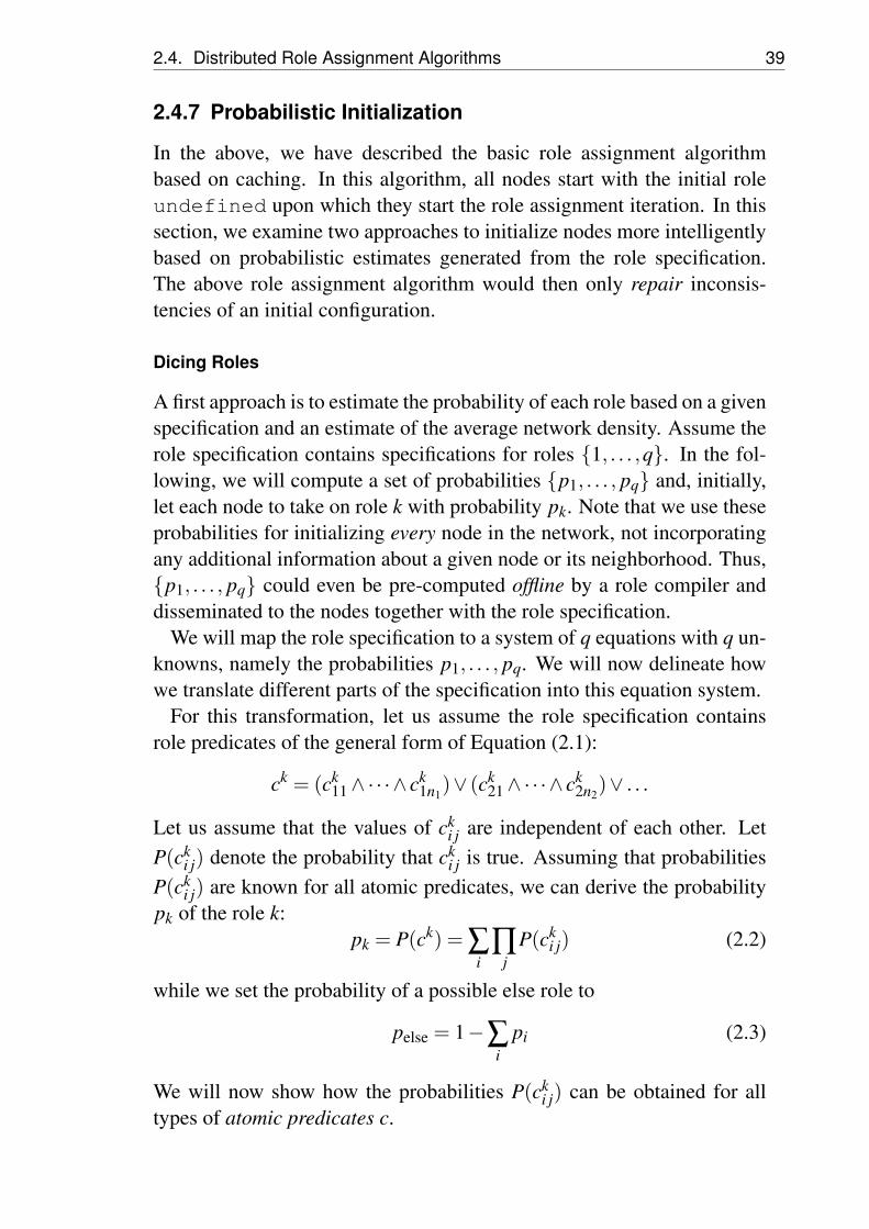
2.4. Distributed Role Assignment Algorithms 39
2.4.7 Probabilistic Initialization
In the above, we have described the basic role assignment algorithmbased on caching. In this algorithm, all nodes start with the initial roleundefined upon which they start the role assignment iteration. In thissection, we examine two approaches to initialize nodes more intelligentlybased on probabilistic estimates generated from the role specification.The above role assignment algorithm would then only repair inconsis-tencies of an initial configuration.
Dicing Roles
A first approach is to estimate the probability of each role based on a givenspecification and an estimate of the average network density. Assume therole specification contains specifications for roles {1, . . . ,q}. In the fol-lowing, we will compute a set of probabilities {p1, . . . , pq} and, initially,let each node to take on role k with probability pk. Note that we use theseprobabilities for initializing every node in the network, not incorporatingany additional information about a given node or its neighborhood. Thus,{p1, . . . , pq} could even be pre-computed offline by a role compiler anddisseminated to the nodes together with the role specification.
We will map the role specification to a system of q equations with q un-knowns, namely the probabilities p1, . . . , pq. We will now delineate howwe translate different parts of the specification into this equation system.
For this transformation, let us assume the role specification containsrole predicates of the general form of Equation (2.1):
ck = (ck11∧·· ·∧ ck
1n1)∨ (ck
21∧·· ·∧ ck2n2
)∨ . . .
Let us assume that the values of cki j are independent of each other. Let
P(cki j) denote the probability that ck
i j is true. Assuming that probabilitiesP(ck
i j) are known for all atomic predicates, we can derive the probabilitypk of the role k:
pk = P(ck) = ∑i
∏j
P(cki j) (2.2)
while we set the probability of a possible else role to
pelse = 1−∑i
pi (2.3)
We will now show how the probabilities P(cki j) can be obtained for all
types of atomic predicates c.

40 Chapter 2. Generic Role Assignment
Let us first consider the case, where c is a simple predicate. If c is ofthe form role==r then P(c) = pr. In all other cases, we require theprogrammer to explicitly specify P(c). This is often possible, as we areonly interested in the probabilities at startup. For example, the probabilityfor the predicate battery>10% can be approximated with 1 at deploy-ment time. Otherwise, an educated guess may be applied. The respectiveprogrammer-specified P(ck
i j) are distributed along with the specification.For count and retrieve predicates, we assume that the average network
density is known and that a function E(h) for the expected number ofnodes within h hops (the so-called h-neighborhood) can be estimated fromdeployment parameters1.
Now consider a count predicate c of the form:
count(scope) { pred } rel lim
where the nested predicate pred is in disjunctive normal form and con-tains only simple sub-predicates ck
i j. That is, we can compute ppred =P(pred) according to Equation 2.2. Let us now consider the case whererel is “<=”, the other cases can be solved in similar ways.
Estimating the number of nodes n to be expected within scope byn = E(scope), we can now formulate the probability that x out of n nodesmatch pred using the binomial distribution:
P(x of n nodes match) =(
nx
)px
pred(1− ppred)n−x (2.4)
Thus, the probability that less or equal lim nodes match pred (and thusthe above count predicate c is true) corresponds to the sum the aboveprobabilities for all x ≤ lim :
P(count = true) =lim
∑x=0
(nx
)px
pred(1− ppred)n−x (2.5)
Finally, a retrieve predicate c of the form
p == retrieve(scope,size) { pred }
requires that at least size nodes exist within scope that match the givennested predicate pred. For calculating role probabilities, we thereforeconsider an equivalent count statement:
count(scope) { pred } >= size1In our implementation, we estimated E(h) for unit disk graphs and random uniform node deployment
on a plane. By fitting results of simulations we found that for any fixed node density E(h)∼ h2.

2.4. Distributed Role Assignment Algorithms 41
So far, we have derived q equations with q unknowns by substitutingP(ck
i j) in Equation (2.2) for 1 ≤ k ≤ q. We use a fixpoint iteration tosolve this equation system. Assume a set of probabilities for each rolepk(t) are known at a given step t. Substituting these into the right side ofequation (2.2), we can compute a set of new probabilities pk(t + 1). Toavoid oscillations in this series, we add a memory term pk(t) that averagesthe old values into the newly chosen ones:
pk(t +1) :=12
pk(t +1)+12
pk(t) (2.6)
Note that at each step, we also normalize the pk(t +1) such that ∑k pk(t +1) = 1. We initialize this series with equal probabilities for each rolepk(0) := 1/q and iterate until the series converges to a fixpoint. We wouldlike to emphasize that this computation is done offline by the role compileras all information needed is the specification and the mentioned estima-tion of the neighborhood size E(h). The resulting probabilities are thenflooded along with the specification upon which each node draws rolek with probability pk and then starts initialization as described in Sec-tion 2.4.2.
We will show in Section 2.6 how the probabilistic initialization can pro-vide significant improvements over the baseline algorithm where all nodesstart with the role undefined.
One Wave
In the above approach we approximate retrieve statements with countoperators ignoring the fact that the local node sets bound by retrievestatements occur in other predicates of the specification. Hence, sub-predicates are not independent of each other (as we assumed).
Furthermore, the result of a retrieve statement depends on the proper-ties of remote nodes. However, the initialization of local properties (thatare usually set by retrieve statements) cannot be performed probabilisti-cally (at least it is highly unlikely that such initialization will be correct).Therefore, additional interaction to adequately initialize such local prop-erties will be required.
In this regard, partial (deterministic) information is helpful and can beused to properly initialize the properties bound by retrieve statements,while other decisions can still be performed probabilistically. In this sec-tion we describe how we can use conditional probabilities to improve thestability of probabilistic decisions.

42 Chapter 2. Generic Role Assignment
The basic idea for this approach is to leverage an existing network flood(e.g., for delivering the role specification) and execute the algorithm ofSection 2.4 while forwarding this “propagation wave”.
We generate such a propagation wave by scheduling the property prop-agation procedure of Section 2.4.3 differently: The sink is the onlynode that initially sends an update message (other nodes refrain fromsending update messages before they received one). A node that re-ceived an update message, awaits a random propagation delay twaveprop ∼(0,Twaveprop), then chooses its role (see below) and includes its own cho-sen role into the forwarded update message. Note that all information ofthese update messages can be piggybacked onto flooded role specificationmessages.
Let us consider the evaluation of the count predicate used as an examplein the previous Section 2.4.7:
count(scope) { pred } <= lim
Figure 2.5 depicts the situation, where the propagation wave reaches agiven node A. Let us assume that A expects n nodes in scope and mof these are behind the wave front (to the left of A). These have alreadychosen their roles and included all relevant information (including theselected role) in previous update messages. That is, A has received updatemessages from all nodes behind the wave (on the left). A will now decideprobabilistically what it expects from the n−m nodes on the right.
information on m nodes
available
n-m more
nodes expected
A
out of m nodes, m‘
nodes match pred
total of n nodes
expected in scope
wave front
Figure 2.5: Propagation wave
For this, let us assume that out of the m known nodes on the left, m′
match the nested predicate pred. We can now reformulate the proba-bility that the count predicate is satisfied as the probability that lim−m′

2.5. Development Environment 43
“more” nodes match (out of the n−m expected nodes on the right). Theconditional probability that the count predicate c is true can be expressedas follows:
P′(c) =lim−m′
∑x=0
(n−m
x
)px
pred(1− ppred)n−m−x (2.7)
Note that count statements using other relations (greater or equal to a con-stant) can be treated analogously, and also the aspect that retrieve state-ments require a minimum number of matching nodes.
When evaluating a retrieve predicate, the node additionally binds thelocal properties to a set of nodes that are known to match the nested pred-icate, if such a set of the required size exists. If such a set exists, weconsistently reflect the dependency between the local node and remotenodes (in our case the remote nodes behind/left of the wave).
For sub-predicates c in pred of the form role==r we still assign thecorresponding pre-computed probability P(c) = pr of Section 2.4.7 as noadditional information is available on the n−m remote nodes that are infront of the wave.
This way, we derive q equations for the conditional probabilities p′k,one for each role similar to Equation (2.2), but formulated in terms of thepreviously computed pk.
p′k = P′(ck) = ∑i
∏j
P′(cki j) (2.8)
What we changed is the way we obtain probabilities P′ for the atomicpredicates ck
i j of the equation. On the nodes, we compute the values ofp′k in one step (without the need for fixpoint iteration) using the {pk}sent along with the specification and choose role k with the respectiveprobability p′k.
The advantage of the above algorithm is that role assignment can beperformed almost entirely within one network-wide flood and that onlyfew role assignments have to be “fixed” later on (using the baseline al-gorithm). Moreover, this approach is able to capture interdependenciesbetween atomic predicates better. We will analyze the performance ofthis algorithm in Section 2.6.
2.5 Development Environment
Generic role assignment is implemented within a development environ-ment which allows programmers to test their specifications with different

44 Chapter 2. Generic Role Assignment
kinds of network topologies before deploying them into operative net-works. The development environment consists of a compiler for rolespecifications, a network setup and configuration component, a visual-ization tool for introspecting algorithm execution and results, and finallytwo back-ends that perform role assignment on the generated topology.The first back-end is a discrete event simulator that executes the presenteddistributed algorithms in a network environment using additive interfer-ence models and realistic wireless parameters. The second back-end is asolver-based analysis tool that can compute optimal role assignment so-lutions in a centralized manner.
Figure 2.6: Role assignment simulation tool
The user interface is shown in Figure 2.6. It allows users to set up anetwork topology, define property directory contents (i.e., the actual nodeparameters) and select the algorithms for execution on the nodes. The rolecompiler then translates a given specification – in this case the clusteringspecification of Section 2.3.1 – into the corresponding syntax tree, per-forms necessary pre-processing and context checking (i.e., ensures thatthere are no circular dependencies and rearranges the role predicates intodisjunctive normal form) and computes a number of additional parameters(such as role probabilities). Syntax tree and parameters are then encoded

2.5. Development Environment 45
into a role specification message, which is then interpreted on the simu-lated nodes.
Finally, the user can trigger delivery of the role specification messagethrough a flood initiated at the network base station, upon which the net-work nodes initialize and execute the role assignment algorithm.
The visualization tool enables qualitative assessment of the algorithmexecution and of role assignment results. Figure 2.6 shows exemplaryresults when using the one-wave variant of the cache table algorithm toimplement the clustering specification introduced in Section 2.3.1. Thehighlighted edges are drawn between a gateway and the clusterheads itconnects. Note that in the shown simulation, apart from messages lostdue to collisions, an additional packet loss probability of 10% was en-abled, which might have caused some – but only few – inconsistent roleassignments. We will discuss quantitative results in Section 2.6.
We use the discrete event simulator JiST/SWANS [Bar04] as a simu-lation back-end. We adopted wireless transmission parameters from theCC1000 radio [CC04] that is in use on the BTnode [BTn06] platform, onMica motes, and on many other platforms, please consider Figure 2.7(a)for details. The physical layer supports additive interference and two-rayfading. Using these parameters we obtain a maximum transmission rangeof about 33 m.
Parameter Valuebandwidth 38.4 kbit/stransmit power 5 dBmsensitivity −96 dBmreceive threshold −84 dBminterference limit −96 dBmfrequency 868 Mhzantenna gain 0 dBnode height 5 cmmax. transmit range 33.5 m
(a) Wireless parameters
Parameter ValueTprop 3 sTeval 10 sTheartbeat 60 sNheartbeat 3Ttermination 60 sTwaveprop 5 sTmin 1 s
(b) Algorithm timers
Figure 2.7: Simulation parameters
We use a variant of the CSMA MAC described in [WC01] with timersand delays adapted for 38.4 kbit/s. Only the broadcast service is used(i.e., no channel reservations are performed). The MAC does not per-form collision detection, or any other means to improve robustness. Wedeliberately chose such a simplistic MAC to study the robustness of ouralgorithm separately from “tricks” performed by more advanced MAC
46 Chapter 2. Generic Role Assignment
layers. The obtained robustness results can be considered “worst case”and better values can be expected when using more sophisticated MAClayers (e.g., [PHC04, vDL03, YHE02]).
The second back-end for role assignment derives an integer linear pro-gram (ILP) formulation from a role specification and a given networktopology. The ILP can provide insights into whether a specification is in-feasible, that is, whether a valid assignment of roles to nodes exists at all.Moreover, it helps assess the quality of the distributed solutions by com-paring them to solutions in which certain sets of roles are minimized ormaximized (e.g., in the coverage example, the solver attempts to choosefewer ON nodes but still cover the respective area). Section 2.8 describesthe solver back-end in detail.
2.6 Evaluation
An important requirement on programming abstractions is that the in-duced overhead should be proportional to the complexity of the specifiedproblem. To gain an insight into whether our algorithms are adaptive inthe above sense, we evaluated three specifications of increasing difficulty:The coverage example that we used to illustrate the caching algorithm inSection 2.4 can be considered a baseline case. Furthermore, we exam-ine aggregation and clustering as defined by the specifications from Sec-tion 2.3.1. These both require propagation of additional properties overtwo hops. The clustering specification is especially challenging throughuse of the retrieve operator that makes role assignment decisions depen-dent on the identities of nodes in the neighborhood.
We will evaluate all three presented algorithms, the baseline cache tablealgorithm from Section 2.4 and its combination with the two probabilisticinitialization schemes described in Section 2.4.7, to which we will referas cachetable, probabilistic and wave, respectively. We set algorithm pa-rameters according to Figure 2.7(b). To evaluate the protocols, we let thethree algorithms assign roles to a previously uninitialized network andstop the simulation if all nodes were stable for Ttermination seconds (eachnode decides termination locally).
We performed experiments on random topologies that are connectedwith high probability. If there should be no multi-hop path from the sinkto a node, this node simply does not participate in the experiment. In ourevaluations, we place a variable number of nodes in a 300 m × 300 msquare field.
2.6. Evaluation 47
For measuring overhead, we consider the total number of messages thatare sent by each node and – as messages can be of variable size – thetotal payload sent by each node in Section 2.6. Note that the numberof messages includes (one) specification message per node, which is theinitial flood.
To quantify correctness of the outcome, we consider the (theoretical)network topology where two nodes have a direct network link if their dis-tance is less than the maximum transmission range of 33.5m. An assignedrole is considered correct if the respective role predicate matches for theset of neighbors obtained from the above theoretical topology.
Later on we will consider the number of role changes that occur afterinitialization to study convergence of our algorithms. For the probabilis-tic and wave algorithms, we do not count the initial role change that isinduced by the probabilistic decision, as we are interested in the remain-ing inconsistency that has to be repaired. For each data point, we indicate95% confidence levels obtained from repeated simulations on indepen-dently drawn random topologies.
Overhead. We study the communication effort spent by the three pre-sented algorithms. We vary the number of nodes in the confined areato see how increasing node density affects the performance of our algo-rithms. The average number of messages sent per node using each speci-fication are shown in Figure 2.8.
The results of Figure 2.8(a) show that the simplified coverage specifi-cation can be implemented effortlessly by all three algorithms. The maxi-mum of three messages includes the specification flood, the later propaga-tion wave for the wave algorithm (we implemented propagation and rolespecification waves separately), and finally at most one more message thatis used to check whether repairs are needed.
In the aggregation example of Figure 2.8(b), the probabilistic and wavevariants outperform the baseline algorithm. Note that the wave algorithmdoes not perform better than probabilistic. This is due to the aggregationspecification (cf. Section 2.3.1): The wave algorithm can improve per-formance only if it can exploit knowledge about nodes behind the wavefront. For the first count statement of role AGG1, this would require thatSOURCE nodes are behind the wave front. However, the specification fur-ther requires that SOURCE nodes are farther away from the sink than ag-gregators. This is unlikely to happen, because the wave propagates from
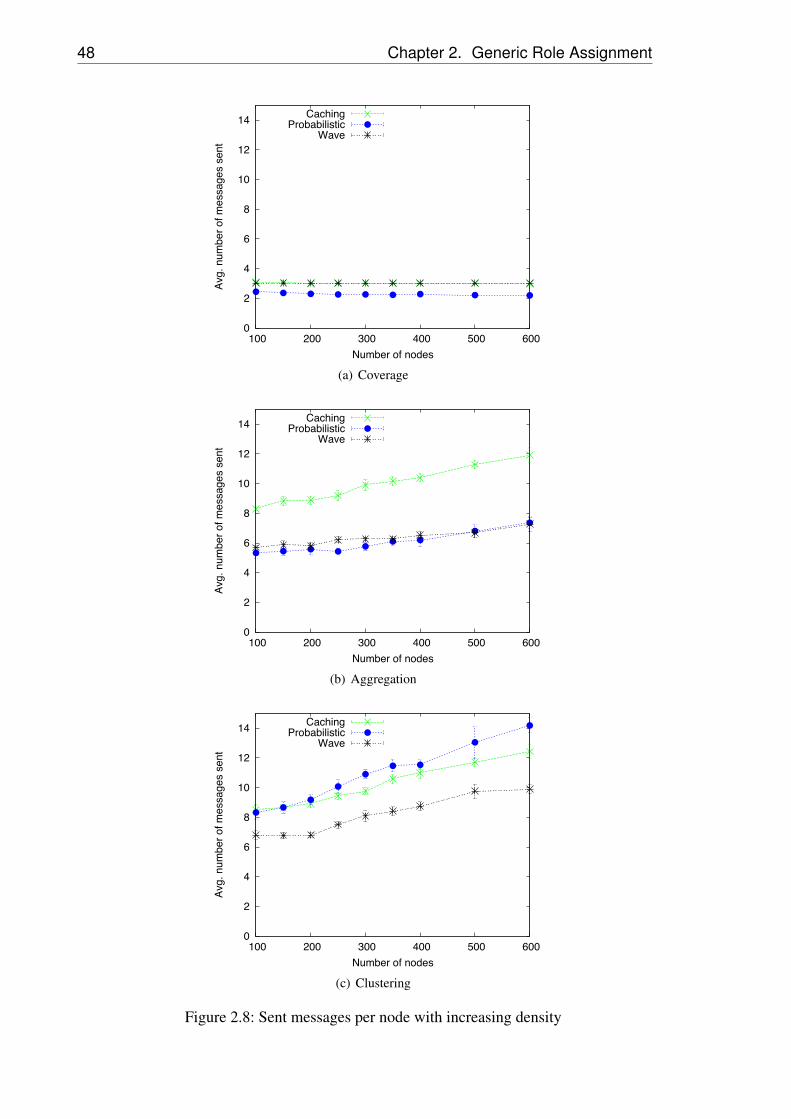
48 Chapter 2. Generic Role Assignment
0
2
4
6
8
10
12
14
100 200 300 400 500 600
Avg
. num
ber
of m
essa
ges
sent
Number of nodes
CachingProbabilistic
Wave
(a) Coverage
0
2
4
6
8
10
12
14
100 200 300 400 500 600
Avg
. num
ber
of m
essa
ges
sent
Number of nodes
CachingProbabilistic
Wave
(b) Aggregation
0
2
4
6
8
10
12
14
100 200 300 400 500 600
Avg
. num
ber
of m
essa
ges
sent
Number of nodes
CachingProbabilistic
Wave
(c) Clustering
Figure 2.8: Sent messages per node with increasing density

2.6. Evaluation 49
the sink outward. Therefore, no aggregator roles are assigned during thefirst wave.
For clustering in Figure 2.8(c), probabilistic performs slightly worsethan caching. This can be explained by the fact that the choice of roleshere depends very strongly on the identities of nodes in the neighborhoodand not only on their roles. Hence it is very unlikely that a probabilisticdecision “guesses” the right node identities, this has been one motivationfor the design of the wave variant, which exhibits better performance.Nevertheless, it is notable that probabilistic still performs comparably tocaching.
The relative performance of the algorithms with respect to payload sizeper node is similar. With the wave algorithm, the total payload size pernode in the clustering example is 179 bytes for 200 nodes and 388 bytesfor 600 nodes, resulting in average message sizes of 26 to 39 bytes, re-spectively. Results are similar in the aggregation case, while coverageonly requires transmitting at most 40 bytes per node as a maximum overall algorithms and node densities. This includes quite high density values:600 nodes in the given area yield an average node degree of around 20.Correctness. We show the fraction of nodes with an incorrect role as-signment in Figure 2.9. The baseline coverage case does not exhibit anysignificant incorrectness. This is due to the simplicity of the specifica-tion, where the count operator considers the 1-hop neighborhood only.Essentially, all nodes send one message to announce their role. If incon-sistencies occur, these are repaired with a second message.
For aggregation and clustering specifications, the caching and wavealgorithms perform best, while the probabilistic variant suffers from itsdeficiencies when used with retrieve operators. Note that even thoughwe omitted any means for reliable message transfer, the wave algorithmachieves very low incorrectness numbers.
Note that shown incorrectness is due to unreliable message deliveryonly. If message delivery were reliable, improbable yet possible simul-taneous role evaluations would not contribute to incorrectness, as thesewould be repaired in subsequent algorithm iterations. Nodes that end upwith incorrect roles have not learned from each other’s properties prop-erly (i.e., at least one message must have been lost). A reliable MAC layerwould incur zero incorrectness but (possibly) worse convergence results.Robustness. To examine robustness in the face of message loss, we in-troduced an additional packet-loss probability. We measured again theratio of incorrect role assignments to the total number of nodes for our

50 Chapter 2. Generic Role Assignment
0
1
2
3
4
5
100 200 300 400 500 600
Inco
rrec
t rol
es in
per
cent
Number of nodes
CachingProbabilistic
Wave
(a) Coverage
0
5
10
15
20
100 200 300 400 500 600
Inco
rrec
t rol
es in
per
cent
Number of nodes
CachingProbabilistic
Wave
(b) Aggregation
0
5
10
15
20
100 200 300 400 500 600
Inco
rrec
t rol
es in
per
cent
Number of nodes
CachingProbabilistic
Wave
(c) Clustering
Figure 2.9: Percentage of incorrect assignments from total nodes with increasing density
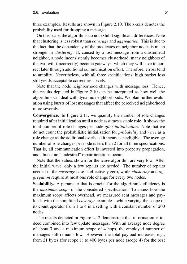
2.6. Evaluation 51
three examples. Results are shown in Figure 2.10. The x-axis denotes theprobability used for dropping a message.
On this scale, the algorithms do not exhibit significant differences. Notethat clustering is less robust than coverage and aggregation. This is due tothe fact that the dependency of the predicates on neighbor nodes is muchstronger in clustering: If, caused by a lost message from a clusterheadneighbor, a node inconsistently becomes clusterhead, many neighbors ofthe two will (incorrectly) become gateways, which they will have to cor-rect later through additional communication effort. Therefore, errors tendto amplify. Nevertheless, with all three specifications, high packet lossstill yields acceptable correctness levels.
Note that the node neighborhood changes with message loss. Hence,the results depicted in Figure 2.10 can be interpreted as how well thealgorithms can deal with dynamic neighborhoods. We plan further evalu-ation using bursts of lost messages that affect the perceived neighborhoodmore severely.Convergence. In Figure 2.11, we quantify the number of role changesrequired after initialization until a node assumes a stable role. It shows thetotal number of role changes per node after initialization. Note that wedo not count the probabilistic initialization for probability and wave as arole change as the additional overhead it incurs is negligible. The averagenumber of role changes per node is less than 2 for all three specifications.That is, all communication effort is invested into property propagation,and almost no “undesired” repair iterations occur.
Note that the values shown for the wave algorithm are very low. Afterthe initial wave, only a few repairs are needed. The number of repairsneeded in the coverage case is effectively zero, while clustering and ag-gregation require at most one role change for every two nodes.Scalability. A parameter that is crucial for the algorithm’s efficiency isthe maximum scope of the considered specification. To assess how themaximum scope affects overhead, we measured sent messages and pay-loads with the simplified coverage example – while varying the scope ofits count operator from 1 to 4 in a setting with a constant number of 200nodes.
The results depicted in Figure 2.12 demonstrate that information is in-deed combined into few update messages. With an average node degreeof about 7 and a maximum scope of 4 hops, the employed number ofmessages still remains low. However, the total payload increases, e.g.,from 21 bytes (for scope 1) to 400 bytes per node (scope 4) for the best

52 Chapter 2. Generic Role Assignment
0
20
40
60
80
100
0 20 40 60 80 100
Inco
rrec
t rol
es in
per
cent
Packet loss in percent
CachingProbabilistic
Wave
(a) Coverage
0
20
40
60
80
100
0 20 40 60 80 100
Inco
rrec
t rol
es in
per
cent
Packet loss in percent
CachingProbabilistic
Wave
(b) Aggregation
0
20
40
60
80
100
0 20 40 60 80 100
Inco
rrec
t rol
es in
per
cent
Packet loss in percent
CachingProbabilistic
Wave
(c) Clustering
Figure 2.10: Robustness in face of dropped packets

2.6. Evaluation 53
0
0.5
1
1.5
2
100 200 300 400 500 600
Avg
. rol
e ch
ange
s pe
r no
de
Number of nodes
CachingProbabilistic
Wave
(a) Coverage
0
0.5
1
1.5
2
100 200 300 400 500 600
Avg
. rol
e ch
ange
s pe
r no
de
Number of nodes
CachingProbabilistic
Wave
(b) Aggregation
0
0.5
1
1.5
2
100 200 300 400 500 600
Avg
. rol
e ch
ange
s pe
r no
de
Number of nodes
CachingProbabilistic
Wave
(c) Clustering
Figure 2.11: Total role changes per node with increasing density
54 Chapter 2. Generic Role Assignment
2
4
6
8
10
12
14
16
1 2 3 4
Avg
. num
ber
of m
essa
ges
sent
Scope of count operator
CachingProbabilistic
Wave
Figure 2.12: Coverage application with increasing scope
performing probabilistic algorithm. With a scope of 4 hops, the averagemessage size is at most 48 bytes.
Summing up, the evaluation results indicate that the role initializationsof probabilistic and wave can provide improvements over the baselinealgorithm. However, we have also seen that there is no single best algo-rithm, although wave outperforms the other algorithms in most settings.With aggregation we found a case, where the wave algorithm is “tricked”by the specification. Apart from such special cases, a rule of thumb isthat wave performs better than probabilistic for specifications that makeuse of retrieve. An interesting direction for future work would bethe development of further heuristics to automatically derive from a givenspecification which algorithm can be expected to give the best results.
2.7 Qualitative Comparison
Throughout the chapter, we have used specific instances of coverage, clus-tering, and aggregation problems to illustrate and evaluate generic role as-signment. In the literature, numerous specialized algorithms for solvingvarious instances of these problems have been proposed. In this section,we discuss how these algorithms compare to our implementations that arebased on generic role assignment.
For each of the problems, we selected a representative instance andalgorithm from literature and discuss differences to our implementationwith respect to semantics and efficiency.
2.7. Qualitative Comparison 55
Coverage. A common semantic for coverage is that all of a node’s sens-ing range should be covered by other sensors before the node can turnoff [TG03]. In our version of coverage we approximate this semantic byturning a node off if there are at least N (we use N = 1 in the example)other on nodes within sensing range. For a more direct implementationof the semantics in [TG03], a node would first retrieve all neighborswith overlapping sensing ranges (i.e., which are at most twice the sens-ing range away) and then use a custom predicate to decide whether allof the node’s sensing range is covered by these neighbors. This spec-ification would require the role assignment algorithm to first propagateposition and role properties across the required number of hops and thenperform local rule evaluation after random delays. Chosen roles wouldbe immediately propagated to affected neighbors. Our algorithm would(quite closely) match the implementation of [TG03] in the variant wheresensing ranges are assumed equal at all nodes. 2
Clustering. Our version of clustering was inspired by (but is not identicalto) passive clustering (PC) [KG02]. With PC, a node declares itself clus-terhead if none of its neighbors have done so before. A node becomes agateway if αCH + β > GW where CH and GW are the numbers of clus-terhead and gateway neighbors, respectively, and α,β > 0 are algorithmparameters that control the desired number of gateways in the system.This approach could be directly implemented by generic role assignmentwith an overhead comparable to the implementation in [KG02], whereonly the role property is shared among neighbors.
With PC, protocol information is piggybacked on existing network traf-fic. In contrast, generic role assignment uses a separate protocol, resultingin some traffic overhead when compared to PC. An interesting directionfor future work would be passive generic role assignment, where protocolinformation would be piggybacked as with PC. 2
Aggregation. A common optimization criterion for aggregator placementis to minimize the total network traffic, which is identical to solving theSteiner-tree problem. Various heuristics are used in the literature to ap-proximate this NP-hard problem. One commonly used heuristic is calledcenter at nearest source [IEGH02], where among a number of neighbor-ing source nodes, the one closest to the sink is selected to act as an aggre-gator. This approach can be implemented with generic role assignment,where a node would use count to decide whether there is another sourcein the neighborhood that is closer to the sink. The scope of count (i.e.,size of the considered neighborhood) would be tuned to achieve a reason-

56 Chapter 2. Generic Role Assignment
able trade-off between algorithm overhead and optimality of aggregatorselection.
If geographic positions are used, the implementation of closer isstraightforward by propagating the position property of a node within thescope. In the original algorithm in [IEGH02], this is done by a network-wide flood. If hop-distance to the sink is used instead of geographic posi-tions, an additional role specification would be needed to obtain the hop-distance of each node from the sink. For this, each node would have aproperty dist that specifies its distance from the sink. A node wouldthen retrieve among its neighbors the node with the smallest distvalue and set its dist property to the retrieved value plus one. Thiswould require a simple extension of the retrieve operator to sort theretrieved nodes according to some user-specified criterion (e.g., minimumof a property value). Note that other, custom-implemented, componentsthat determine the dist property could be integrated with role assign-ment via the property directory. 2
Apart from the above specific examples, we can make some more generalobservations about the efficiency of generic role assignment when com-pared to specialized algorithms. With generic role assignment, the valueof a property is always propagated to all nodes in the scope of this prop-erty. In some cases, however, it may not be necessary to propagate certainproperty values. In other cases, certain nodes may not need to propa-gate a property at all or only to certain nodes within a scope. As part offuture work we will investigate whether such optimizations can also besupported by generic role assignment.
2.8 Role Assignment Solver
In the previous sections, we have mentioned a couple of open issues withthe described generic role assignment system. The first of these issues istermination. For specifications, for which no assignment of roles to nodesexists that satisfies all rules, our distributed algorithms may not converge.Therefore, mechanisms are needed that assist developers with detectingsuch faulty specifications. The second open issue is that many practicalrole assignment problems include some global optimization criteria, suchas the minimization of the number of ON nodes in the above coverageproblem. Such problems cannot be expressed with the role specificationsyntax from Section 2.3.2.
2.8. Role Assignment Solver 57
The role assignment solver provides an analysis tool for approachingthese issues. In addition to the syntax specified in Section 2.3.2, the solvercomponent allows developers to specify global optimization criteria of theform min role or max role, where role can be any of the roles thathave been defined, for example:
min ON
Multiple such specifications may be issued alongside a role assignmentspecification to demand minimization or maximization of the respectiveset of roles. The complete role specification and a given network topol-ogy are then used as input to the role assignment solver. Given such input,the solver will compute a role assignment taking into account the speci-fied optimization criteria, or state infeasible if no feasible role assignmentexists.
The remainder of this section is structured in two parts. First, in Sec-tion 2.8.1, we provide a mapping of the role specification language to Inte-ger Linear Programs (ILP). This mapping, performed within the develop-ment environment described in Section 2.5, returns a problem formulationthat can be used as an input to the CPLEX commercial solver. Second, inSection 2.8.2, we use the resulting ILPs and CPLEX to re-examine someof the role assignment specifications presented in Section 2.3. In partic-ular, we show how infeasible (non-terminating) specifications can be de-tected, and quantify improvements that can be achieved by using globaloptimization criteria.
2.8.1 Integer Program Mapping
An instance of a role assignment problem consists of a role specification(a set R of role predicates according to the syntax described in Section2.3), all property values of all nodes that are referenced by the role speci-fication, and a sensor network graph G = (V,E) with n = |V | participatingnodes.
G is used to define the elements of the h-hop neighborhood matricesA(h) as follows:
A(h)i j =
1 ∃ path from node i to node j
with length ≤ h0 otherwise
The mapper generates a total of h = 1 . . .S such matrices, where S de-notes the maximum scope that occurs in all count and retrieve statements
58 Chapter 2. Generic Role Assignment
of a specification. Note that these matrices can be readily computed fromthe graph G’s adjacency matrix A(1). The above notation A(h)
i j will be usedto formulate the ILP constraints of count and retrieve operators in SectionMapping Predicates below.
Role Assignment Variables
We first introduce the variables we use to encode the solution of a genericrole assignment problem. Unless otherwise noted, all variables are binarywith values ∈ {0,1}.
The first set of binary variables xik is used to encode whether a node isatisfies the predicate ck of a given role k:
xik =
{1 if node i satisfies ck
0 otherwise(2.9)
By ck we refer to the Boolean predicate describing the conditions for as-suming role k as discussed in Section 2.3.2. We will ensure that (2.9)holds by translating ck into a set of equivalent constraints on xik below.
Furthermore, we require that at least one role predicate (from the set ofdefined roles R) must match for every node, otherwise, the role assign-ment is not feasible. This gives rise to the constraint
∑k∈R
xik ≥ 1 ∀ nodes i . (2.10)
Note that, in order to avoid infeasibility, the programmer can alwaysspecify an else role q which does not imply any constraints as it doesnot have any sub-predicates (see Section 2.3.2). Therefore, the predicateof an else role would always be satisfied, and, according to the abovedefinition (2.9), a solution should always set xiq to 1.
This points to a different aspect of the variables xik: The propertiesand network neighborhood of a given node i could satisfy the conditionsfor more than one role, as we do not require the programmer to specifydisjunct conditions in the predicates ck. Therefore, more than one ck canbe satisfied, requiring – because of (2.9) – that more than one xik is set to1 for a given node i. Thus, the variables xik cannot directly be used as anoutput variables of the role assignment solver.
Instead, the output variables should follow the semantics of the dis-tributed algorithms of Section 2.4, namely, roles defined earlier in the
2.8. Role Assignment Solver 59
specification should be given priority over later ones if multiple role pred-icates match. These semantics imply that the first matching role withxik = 1 is assigned to a node i. This is implemented using an additionalset of binary result variables yik which we require to be 1 only if the condi-tions for roles 1, ...,k−1 (i.e., roles specified prior to k) are not satisfied.Here we assume that k denotes role k’s position in the list of roles speci-fied by the programmer (we can achieve this by simply re-numbering theroles). The following constraint formulates the necessity that yik mustequal 1 (i.e., the role must be assigned) if the given role predicate is true(xik = 1) and at the same time all predicates stated earlier in the role listare false (∑k−1
l=1 xil = 0):
xik−k−1
∑l=1
xil ≤ yik ∀k, i (2.11)
Vice versa, in an additional constraint (2.12), we require that role k canonly be assigned if the corresponding predicate is true (xik = 1). Further,(2.13) requires that exactly one role from the role set R should be assigned.
yik ≤ xik ∀k, i (2.12)
∑k∈R
yik = 1 ∀i (2.13)
Finally, we introduce binary variables for node sets p that are bound tothe results of retrieve predicates of the form
p == retrieve(scope,size) { pred } .
For each such set p, we include an additional set of variables qpi ( j) with
j ∈V with the following interpretation:
qpi ( j) =
{1 if the set p at node i contains node j
0 otherwise(2.14)
To preserve a readable notation, we will sometimes omit the index p andjust write qi( j) implicitly referring to the respective set p.
Objective Function
We can now reformulate the optimization criteria of the form max roleor min role into an objective function in terms of the variables yik. As-sume that out of a set of roles R stated in a given role assignment specifi-
60 Chapter 2. Generic Role Assignment
cation, the user would like to minimize the set of roles m ⊂ R and maxi-mize the set of roles M ⊂ R in the network. The corresponding objectivefunction is
minimize ∑i∈V
(∑k∈m
yik− ∑k∈M
yik
).
Note that one may easily re-state this objective function to formulatemore complex optimization criteria in terms of the variables yik. For ex-ample, one may express the desire to maintain certain ratios between ONand OFF nodes (in the coverage example), or assign weights to the impor-tance of minimizing or maximizing certain roles.
Mapping Predicates
We will in the following show the mapping of role predicates ck to re-spective ILP constraints on the predicate variables xik. Note that the con-straints will depend on i because the network neighborhood is a functionof the node identity i.
Consider a role predicate given in its disjunctive normal form as de-scribed in Section 2.3.2
ck = (ck11∧·· ·∧ ck
1n1)︸ ︷︷ ︸
ak1
∨(ck21∧·· ·∧ ck
2n2)︸ ︷︷ ︸
ak2
∨·· · . (2.15)
As a first step, we translate the Boolean operations to ILP constraintsby means of a (standard) ILP modeling technique. For this purpose, weuse additional indicator variables ui(c) which (similarly to xik) indicatewhether an atomic predicate c occurring anywhere in (2.15) is satisfied ata given node i.
Disjunctions and conjunctions can be expressed in terms of ILP con-straints as follows. Assume a conjunctive term of the form (c = c1∧·· ·∧cp), consisting of p terms, and let ui(c1) . . .ui(cp) be the respective in-dicator variables for a given node i. We will use an additional variableui(c) to indicate whether the whole conjunction c is true. We thereforerequire (for every node i) that ∑ui(cq) ≥ p if and only if ui(c) = 1. The
2.8. Role Assignment Solver 61
constraints modeling necessity and sufficiency are:p
∑q=1
ui(cq) ≤ ui(c)+ p−1
p
∑q=1
ui(cq) ≥ p×ui(c)
∀i (2.16)
Similarly, for an analogous disjunction of the form a = a1∨ ·· · ∨ ap, werequire that at least one of the indicator variables ui(aq) of a node i is 1,thus ∑ui(aq)≥ 1 if and only if ui(a) = 1, for all nodes i. The constraintsmodeling necessity and sufficiency are:
p
∑q=1
ui(aq) ≤ p×ui(a)
p
∑q=1
ui(aq) ≥ ui(a)
∀i (2.17)
We will use (2.16) and (2.17) on several occasions when we need to modelconjunctions or alternatives. Once conjunctions and alternatives can bemodeled, the remaining task is to map the atomic predicates ck
qr of (2.15)to constraints on their respective indicator variables ui(ck
qr). This map-ping is implemented in various ways depending on the type of the atomicpredicate.Simple Predicates. We begin with simple predicates c that are local inthat they refer only to the properties of a given single node. These are for-mulated in terms of property values of the node – which are, essentially,known constants – and can therefore be evaluated before generating theILP. Hence, the respective indicator variable ui(c) can simply be replacedby either 0 or 1.
Simple predicates that are nested in count or retrieve statements arespecial cases that will be considered under nested predicates below.Count Predicates. Consider a count predicate c of the form:
count(scope) { pred } <= lim
In the following we formulate equivalence between ui(c) = 1 and c. Letu(pred)j be the variable indicating whether pred is true at a node j. Weconstrain ui(c) as follows to formulate the necessity that (ui(c) = 1)→ c,
∑j 6=i
A(scope)i j u(pred)j ≤ (1−ui(c))M +lim (2.18)
62 Chapter 2. Generic Role Assignment
where M is a constant value greater than the total number of nodes n. Notethat the above reduces to either (2.19) or (2.20) if the indicator ui(c) is 1or 0, respectively:
∑j 6=i
A(scope)i j u(pred)j ≤ lim (2.19)
∑j 6=i
A(scope)i j u(pred)j ≤ M +lim (2.20)
The former case (2.19) exactly formulates the semantics of the abovecount predicate c, namely that the number of nodes j within scope thatmatch pred should be less or equal to lim. In the latter case (2.20), theconstraint is nullified by M, as M > n and the left-hand sum will never belarger than the number of nodes.
The above equations (2.19) and (2.20) formulate the necessity thatui(c)→ c. In a second step, we formulate the sufficiency c→ ui(c), equiv-alent to ui(c)∨¬c, using the constraint
∑j 6=i
A(scope)i j u(pred)j ≥ (lim+1)(1−ui(c)) (2.21)
which requires ¬c if ui(c) = 0 while imposing only a trivial constraint ifui(c) = 1. In summary, the constraints (2.18) and (2.21) model a countoperator that uses the relation ≤. Note that count operators using otherrelations can be treated analogously.Retrieve Predicates. A retrieve predicate c of the form
p == retrieve(scope,size) { pred }
evaluates to true if all of the following three requirements are met.First, at least size nodes must exist within scope that match the given
nested predicate pred. We model this requirement as a count statementof the form
count(scope) { pred } >= size
Second, we must ensure that every retrieved node j that is in the set p ofnode i really is in scope and also matches the predicate pred
qpi ( j)≤ A(scope)i j u(pred)i . (2.22)
Third, we require that the number of elements in the set p is size
2.8. Role Assignment Solver 63
n
∑j=1
q(p)i ( j) = size. (2.23)
Finally, we can formulate that u(c) = 1 if and only if all of the aboverequirements hold at the same time using the approach for implementingconjunctions given in (2.16).
Nested Predicates. In the following consider predicates that occur nestedin count or retrieve statements with a given scope.
For a nested predicate c that refers to the role of the node, i.e.,role==k, no separate indicator variable u j(c) is needed. We can insteadre-use the existing result variable y jk which indicates whether the role ofa node j is k.
A special case are simple predicates c that check equality between twoproperties that represent node sets such as
clusterheads == super.clusterheads
in the clustering example.To model set equality, we introduce additional indicator variables Qi j
that are set to 1 if and only if the set clusterheads of node i is equal tothe set super.clusterheads at node j. The interesting case is whenthe two sets are bound by retrieve predicates (as in the above clusteringexample), and thus constitute variables of the algorithm. In these cases,the parameter size of the respective retrieve predicates indicates the sizeof the set (we assume the sets are of equal size, otherwise the compilercan already set u(c) to 0). In all other cases Qi j can be evaluated beforegenerating the ILP and simply noted as 1 or 0, respectively.
In the following, we describe the constraints on Qi j. These are formu-lated in terms of the variables qi(k) representing the set of node i, whereqi(k) = 1 if and only if the element k ∈ {1, ...,n} is contained in the set atnode i, as defined in (2.14). Likewise, respective variables q j(k) for nodej are used. We first compute a set of n helper variables qi j(k) for whichwe require that qi j(k) = qi(k)∧ q j(k) using equation (2.16). Figure 2.13shows an example with two sets of size 2 in which black circles indicatethat the respective q∗(k) = 1.
Using qi j(k), we can formulate that variables Qi j should be 1 if theintersection of the sets at node i and j contains at least size elements(i.e., if the sets are equal):

64 Chapter 2. Generic Role Assignment
of node
( )iq k( )jq k
( ) ( ) ( )ij i jq k q k q k= ∧
n
ij
additional helper variables
of node
1,k = 2, …3,
Figure 2.13: Set equality
n
∑k=1
qi j(k)≤ Qi j−1+size (2.24)
Otherwise, Qi j should be 0:
n
∑k=1
qi j(k)≥ size×Qi j (2.25)
Finally, we can replace u j(c) that occur nested within a count orretrieve statement of a given node i by the corresponding Qi j.
Complexity
Depending on the complexity of the role specifications, the resulting ILPsare solvable in reasonable time for up to 1000 nodes using the CPLEX
[CPX] commercial solver. Some specifications, however, can result inrather large ILPs with many indicator variables and constraints. This isparticularly the case with specifications that contain retrieve predicates.Below we therefore analyze how the above mapping could be imple-mented using a much lower number of variables – an improvement whichwe have so far omitted for ease of exposition. The number of variablescan be used as an indicator for the compute time of a generated ILP.
In the above, we used a total number of n×m variables to encode thebasic role assignment decision, where m denotes the number of specifiedroles and n denotes the number of nodes in the network. Further, weadded another set of n variables for each node, to encode local propertiescontaining node sets that are bound by retrieve statements, resulting inanother n2×b variables, where b represents the total number of differentnode sets used in the role specification.
Moreover, in the above mapping of role predicates, we introduced anumber of additional indicator variables. A total of n× a variables areused to encode atomic predicates at each node, where a is the number of
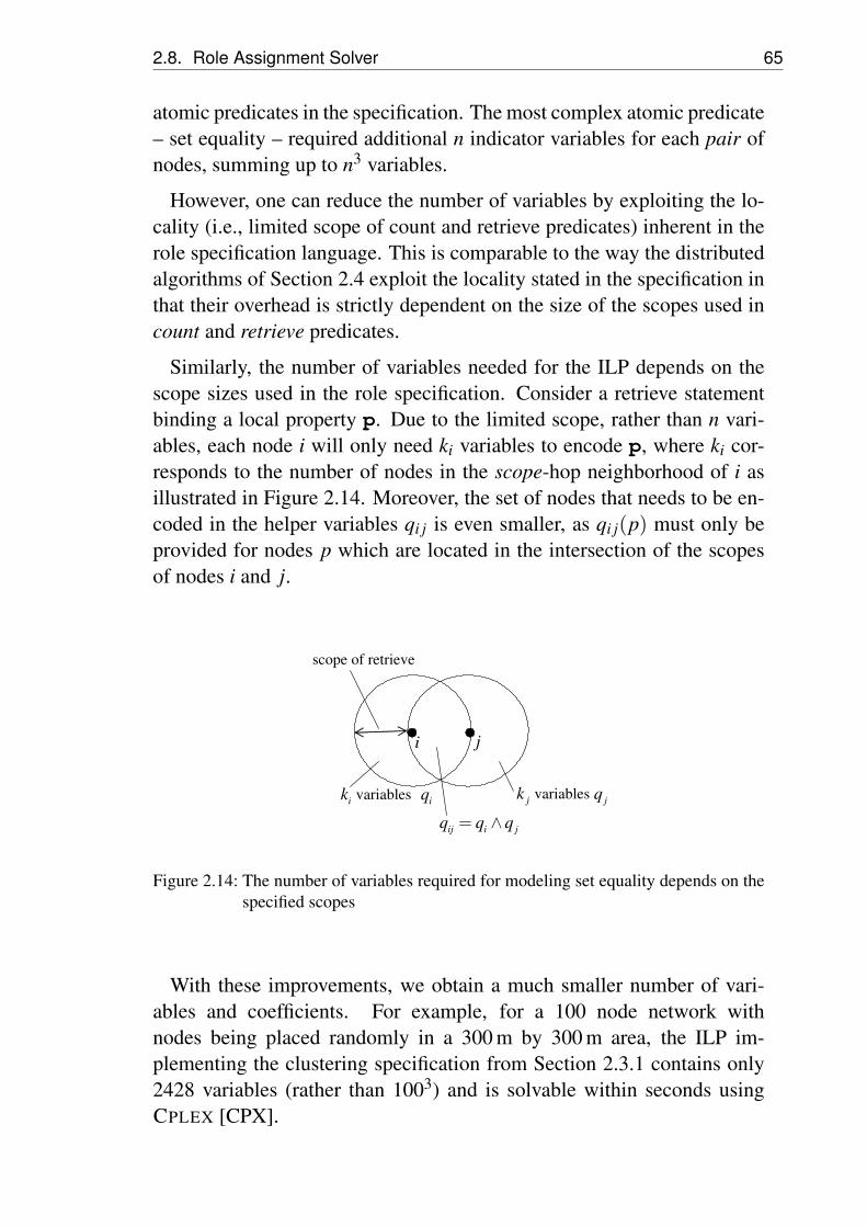
2.8. Role Assignment Solver 65
atomic predicates in the specification. The most complex atomic predicate– set equality – required additional n indicator variables for each pair ofnodes, summing up to n3 variables.
However, one can reduce the number of variables by exploiting the lo-cality (i.e., limited scope of count and retrieve predicates) inherent in therole specification language. This is comparable to the way the distributedalgorithms of Section 2.4 exploit the locality stated in the specification inthat their overhead is strictly dependent on the size of the scopes used incount and retrieve predicates.
Similarly, the number of variables needed for the ILP depends on thescope sizes used in the role specification. Consider a retrieve statementbinding a local property p. Due to the limited scope, rather than n vari-ables, each node i will only need ki variables to encode p, where ki cor-responds to the number of nodes in the scope-hop neighborhood of i asillustrated in Figure 2.14. Moreover, the set of nodes that needs to be en-coded in the helper variables qi j is even smaller, as qi j(p) must only beprovided for nodes p which are located in the intersection of the scopesof nodes i and j.
ik
i j
jkvariables
scope of retrieve
iq
ij i jq q q= ∧
variablesjq
Figure 2.14: The number of variables required for modeling set equality depends on thespecified scopes
With these improvements, we obtain a much smaller number of vari-ables and coefficients. For example, for a 100 node network withnodes being placed randomly in a 300 m by 300 m area, the ILP im-plementing the clustering specification from Section 2.3.1 contains only2428 variables (rather than 1003) and is solvable within seconds usingCPLEX [CPX].

66 Chapter 2. Generic Role Assignment
2.8.2 Evaluation
We extended the existing role assignment development environment de-scribed in Section 2.5 with the capability of generating an ILP represent-ing the execution of a given specification on a given topology. The gen-erated ILP is formulated using the ZIMPL [Koc05] modeling language,which we use as a front end for the CPLEX solver. Finally, the develop-ment environment visualizes the ILP’s results on the respective networktopology.
Using the above ILP mapping of role specifications, we can re-examinethe role assignment specifications regarding their optimality, feasibilityand termination, which were open problems so far.
One new aspect of the generated ILP is that it enables the programmerto express a desired optimality goal, i.e., to minimize or maximize thenumber of nodes that are assigned a certain role. While the existing spec-ifications were not devised with a possible optimization in mind – rather,these were designed as input for distributed algorithms which assign rolesin a greedy fashion –, it is nevertheless interesting how the optimal resultscompare to the ones found using the distributed algorithms of Section 2.4.
As illustrated in Figure 2.15, we examined the minimum number of ONnodes required to ensure coverage based on the coverage specification thatwas used in the evaluation of our distributed algorithms in Section 2.6. Asin earlier evaluations, nodes with a communication range of around 33 mwere randomly distributed in a square area of 300 m by 300 m.
Previously, we studied the same specification with several distributedalgorithms (caching, probabilistic and wave) in terms of their efficiencyregarding communication traffic, but did not employ any strategy to min-imize the number of ON nodes. It is therefore not surprising that the ILPapproach can yield solutions with about half as many ON nodes as thedistributed algorithms.
As mentioned, the distributed algorithms assign roles in a greedy fash-ion and do not attempt any optimization. If developers are interested toimprove the quality of the results obtained by the distributed algorithms,they may add additional conditions to the role specifications (using theoriginal specification techniques of Section 2.3). In this regard, the op-timal solution obtained via the ILP indicates the room for potential im-provement using more refined role specifications.
Moreover, the role assignment solver can provide interesting insightsinto undesirable effects of a role specification. While the clustering spec-

2.8. Role Assignment Solver 67
0
50
100
150
200
200 250 300 350 400 450 500 550 600
ON
nod
es
Number of nodes
CachingProbabilistic
Wave ILP
(a) Increasing node density
0
5
10
15
20
25
30
35
40
45
50
1 1.5 2 2.5 3 3.5 4
ON
nod
es
Scope of count operator
CachingProbabilistic
Wave ILP
(b) Increasing scope
Figure 2.15: Number of ON nodes in simplified coverage example
ification (re-stated in Figure 2.16 for convenience), when interpreted bythe distributed algorithms, typically results in a connected backbone net-work of clusterheads and gateways (Figure 2.17(b)), minimizing both theCH and GW roles results in a set of isolated clusters (Figure 2.17(a)), whichare usually not desirable in practical applications. The optimized assign-ment places clusterheads exactly three hops away from each other, thusensuring that each slave is a neighbor of at least one clusterhead, whileat the same time avoiding assignment of the gateway role (as hardly anynode has more than one clusterhead neighbor). This hints at a weaknessof the specification, namely that it does not enforce that clusterhead andgateway nodes should provide a connected backbone.
For the case that clusterhead and gateway roles are maximized, an ex-emplary solution is shown in Figure 2.17(c). Here, clusterhead nodes areexactly two hops away and arranged in an ordered fashion that allowsfor many gateway nodes. Essentially, Figures 2.17(a) and 2.17(c) show
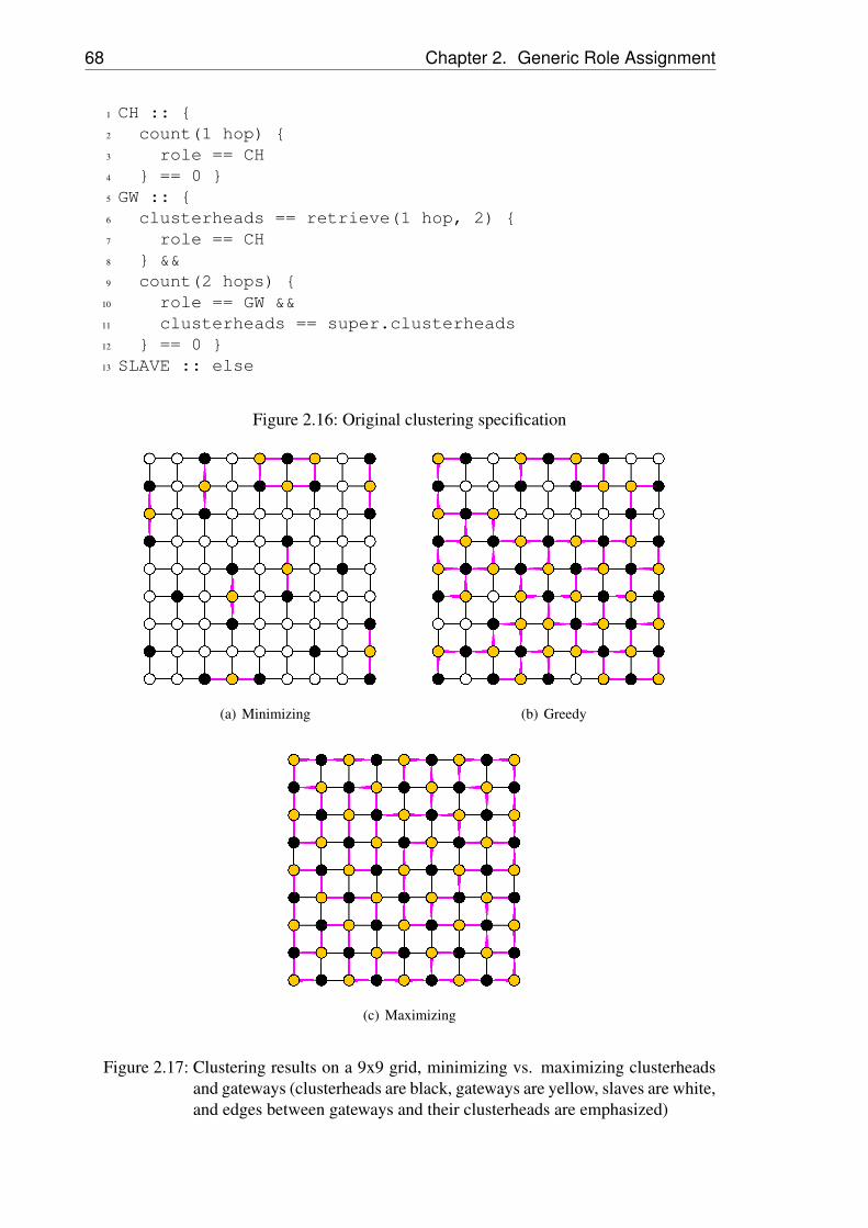
68 Chapter 2. Generic Role Assignment
1 CH :: {2 count(1 hop) {3 role == CH4 } == 0 }5 GW :: {6 clusterheads == retrieve(1 hop, 2) {7 role == CH8 } &&9 count(2 hops) {
10 role == GW &&11 clusterheads == super.clusterheads12 } == 0 }13 SLAVE :: else
Figure 2.16: Original clustering specification
(a) Minimizing (b) Greedy
(c) Maximizing
Figure 2.17: Clustering results on a 9x9 grid, minimizing vs. maximizing clusterheadsand gateways (clusterheads are black, gateways are yellow, slaves are white,and edges between gateways and their clusterheads are emphasized)

2.8. Role Assignment Solver 69
two extremal outcomes that may occur with the current clustering speci-fication – hinting the developer that there is a potential problem with thisspecification.
The clustering specification performs more accurately with distributedalgorithms that greedily assign roles as seen in Figure 2.17(b) – as it wasoriginally designed as an input to these algorithms. With their semantics,the clustering specification results in a connected backbone in most cases.However, there is no guarantee that the backbone is always connected.We therefore discuss a set of specification heuristics that overcome thisweakness in Section 2.9 below.
Enabling the programmer to formulate an additional constraint, namelythat a set of roles should be connected, would be an interesting exten-sion for the solver component. Such a feature would complement relatedwork [MLM+05] which estimates whether a set of roles would form aconnected backbone in the average case.
Finally, the ILP translation helps to better understand erroneous spec-ifications that do not terminate when using the current distributed algo-rithms. Consider the mentioned RED-GREEN example for which the dis-tributed algorithms of Section 2.4 would change back and forth betweenthe roles RED and GREEN:
1 RED :: { count(1) { role == GREEN } >= 1 }2 GREEN :: { count(1) { role == RED } <= 0 }
Using the ILP mapping of the above specification we could show that thespecification is in fact infeasible – that is, no solution of the generated ILPexists – on a range of different network topologies.
Apart from evaluating feasibility on a given network graph, we can alsoreformulate the ILP to check whether, given a certain number of nodes,there exists any network graph for which the problem has a solution. Bydoing so for the above specification, we obtained graphs consisting ofsingle isolated GREEN nodes as the only feasible combination of networktopology and role specification. When adding the (practical) requirementthat every node should have at least one neighbor, no solution can befound, indicating that the specification is infeasible on any reasonablenetwork topology.
For illustration of this result, consider the simplest graph with two nodesu, v and an edge (u,v) as shown in Figure 2.18. Looking carefully, we cansee that, out of the 4 assignments that are possible in this graph, none isfeasible. While the last example (both nodes green) seems feasible at first,

70 Chapter 2. Generic Role Assignment
Green
Red
Figure 2.18: RED / GREEN example: None of the four possible role assignments satisfiesthe role specification
it is not: As both nodes also match the predicate for RED, the assignmentdoes not comply with the requirement that the first matching role shouldbe assigned.
This example suggests that there is a close relationship between specifi-cations that do not terminate when executed by the distributed algorithmsand specifications that result in infeasible ILPs. What is certain is thatinfeasible specifications cannot provide any correct result with the dis-tributed algorithms, and should therefore be discarded before distributingthem to the network.
Unfortunately, it is uncertain whether a complementary claim alsoholds, namely, that one feasible solution implies fast convergence of thedistributed algorithms. Nevertheless, there is an argument supporting thisclaim. First, note that the convergence speed is likely to be dependent onthe number of feasible assignments in the network. If the number of fea-sible assignments is very small, the distributed algorithms are unlikely tofind a correct solution. Instead, they will either end up in a partly incom-plete configuration (where some nodes have taken on feasible roles andlater on some nodes are assigned the role undefined as, based on the spec-ification, no feasible roles for them remain), or in an endless iteration (asin the RED-GREEN example). If the number of feasible solutions is large,however, the algorithm is likely to converge to a feasible configurationfast.
In this context, we argue that a feasible specification will usually havemany feasible solutions, not just a few. This has to do with the symme-tries of the system, which are caused by the fact that the same specifi-cation is distributed to all nodes: If for a given specification at least onefeasible assignment exists on each of a range of different network topolo-gies, these assignments can be shifted, rotated, tiled, or combined into aplethora of feasible solutions. This argument is consistent with the resultsof our evaluation of the distributed algorithms (Section 2.6), in which theconvergence period always turned out very short.

2.9. Additional Role Specifications and Language Extensions 71
In particular, note how the most useful role assignment specifications(such as the coverage, clustering, and aggregation specifications we eval-uated in Section 2.6) focus on choosing special nodes that perform a spe-cific task (such as the on, clusterhead, or aggregator nodes, respectively).These specifications allow for a particularly high number of feasible solu-tions, because it does not matter which node from a set of network neigh-bors is elected special. Once an arbitrary initial choice of special nodeshas been made, a feasible solution, in which the special nodes’ neighborsare assigned slave or gateway roles, can be found easily.
2.9 Additional Role Specifications and LanguageExtensions
The previous sections have described and evaluated a comprehensive sys-tem for assigning roles to sensor nodes. Based on the role assignmentsolver of the previous Section 2.8, a deficiency of the example specifica-tion we used for clustering has become apparent, namely, that it does notguarantee that clusterhead nodes are connected.
Before concluding this chapter, we therefore briefly discuss a few exam-ples of additional role assignment specifications. These should underlinethe generality of the system and provide important building blocks fromwhich developers can derive their own specifications consisting of com-binations and variations of the specifications provided here.
Further, we discuss a set of refinements of these specifications, whichwe use to point out valuable extensions to the role assignment language.These extensions would be easy to embed into the distributed role assign-ment algorithm and at the same time would make it more flexible andgeneric.Data Gathering Tree. We have mentioned that generic role assignmentcan be used to construct trees. Consider the following simple specifica-tion:
1 CHILD :: {2 parent == retrieve(1 hop, 1) {3 role == SINK ||4 role == CHILD5 }6 DISCONNECTED :: else
The specification requires that CHILD nodes are either neighbors of thenetwork’s sink or of other CHILD nodes. Because all nodes start in an

72 Chapter 2. Generic Role Assignment
undefined role, the role CHILD implies that the node is truly connected tothe sink. Because every node except the sink picks one parent, the abovespecification implements a tree that grows from the sink. The local prop-erty parent is used to retain a node’s parent in the tree and to make itavailable to other applications by means of the node’s property directory.
Note that after constructing the initial configuration, after a failure of aparent node it may happen that CHILD nodes re-connect to other CHILDnodes forming a cycle which is not connected to the sink. This is acommon problem in tree construction protocols and can be addressed byadding a local counter property that stores a node’s hop distance to thesink. Every node would pick a parent whose counter is smaller than itsown and, further, set its own counter to the one of its parent plus one.Such details could be implemented using the syntax we introduce in thissection. Note that we omit these details, when we implement trees in thespecifications below.Connected Clustering. The clustering specification, which we intro-duced in Section 2.3.1, can be enhanced by constructing a tree in a similarmanner.
We mentioned that the original specification does not guarantee thata connected communication backbone of clusterheads and gateways isconstructed. Instead, it relies on heuristic constraints on the gateway rolethat shall provide a connected topology in most cases and yet keep thetotal number of gateway nodes low.
By a slight adaptation of the specification, however, a connected topol-ogy can be obtained. Consider the enhanced clustering specificationshown in Figure 2.19, which only adds the lines 5–8 to the original clus-tering specification introduced in Section 2.3.1:
The additional requirement for the assignment of the clusterhead (CH)role (lines 5–8) is derived from the specification of the CHILD role above.A node is allowed to become a clusterhead only if a “parent” clusterhead(or the sink) is present within two hops of the local node. This way, basedon the provided specification for gateways (GW), later on at least one GWnode will be elected connecting the new clusterhead to its parent.Clustered Tree. The above combination of the tree and clustering spec-ifications hint at a refined version of this specification. For example, thespecification of the gateway role GW still focuses on connecting arbitrarypairs of clusterheads. If a developer, instead, prefers to construct a clus-tered tree rooted at the sink, and does not desire any additional inter-clusterhead gateways, the specification shown in Figure 2.20 can be used.
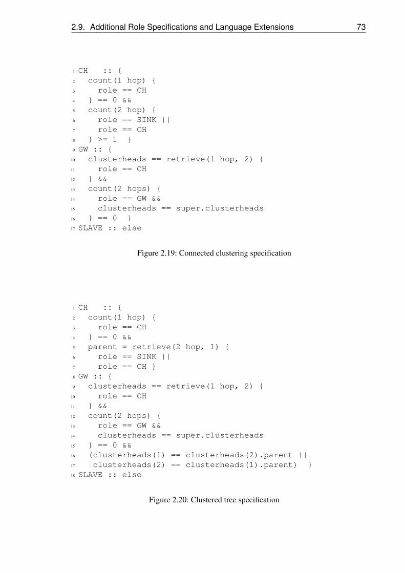
2.9. Additional Role Specifications and Language Extensions 73
1 CH :: {2 count(1 hop) {3 role == CH4 } == 0 &&5 count(2 hop) {6 role == SINK ||7 role == CH8 } >= 1 }9 GW :: {
10 clusterheads == retrieve(1 hop, 2) {11 role == CH12 } &&13 count(2 hops) {14 role == GW &&15 clusterheads == super.clusterheads16 } == 0 }17 SLAVE :: else
Figure 2.19: Connected clustering specification
1 CH :: {2 count(1 hop) {3 role == CH4 } == 0 &&5 parent = retrieve(2 hop, 1) {6 role == SINK ||7 role == CH }8 GW :: {9 clusterheads == retrieve(1 hop, 2) {
10 role == CH11 } &&12 count(2 hops) {13 role == GW &&14 clusterheads == super.clusterheads15 } == 0 &&16 (clusterheads(1) == clusterheads(2).parent ||17 clusterheads(2) == clusterheads(1).parent) }18 SLAVE :: else
Figure 2.20: Clustered tree specification

74 Chapter 2. Generic Role Assignment
Compared with Figure 2.19, line 5 now binds the parent clusterheadin the tree using retrieve. Moreover, an additional requirement hasbeen added to the gateway role GW in lines 16–17. This statement requiresthat among the two clusterheads connected by a potential gateway,the first should be the parent of the second or vice versa. This way, once atree of clusterhead roles has been established – in which clusterheads arealways two hops apart – GW nodes will simply connect the original treeconstructed using the CH role. In this specification, more nodes can beassigned the energy efficient SLAVE role, as much fewer nodes functionas gateways.
The statements in lines 16–17 use an extended syntax to access themembers of the set clusterheads in an ordered manner. This syntaxwould be mapped onto set operations performed by an enhanced prop-erty directory. In order to support the notation used in lines 16–17, theproperty directory must store node sets in some arbitrary order and pro-vide for access to individual elements of these sets. While such featuresare not present in our current implementation, we expect that an existing(and more powerful) property sharing component can be used for thispurpose, especially because various literature has argued for adequatenode-level components that are conceptually similar to our property di-rectory [KHHK04, LMMR05]. Vice versa, many other systems (otherthan role assignment) could benefit from a more powerful implementa-tion of the property directory and, in particular, from data structures thatfacilitate dealing with nodes, sets of nodes, and properties of these nodes.
In the example of lines 16–17, any deterministic ordering of the nodes inthe clusterheads set would suffice (e.g., based on node identifiers).If the developer could additionally specify which node property shouldbe used to impose an order on the nodes in the set, even more powerfulspecifications become possible. In the remaining examples, we will usethe syntax
nodeset(index,prop)
where the above expression references the node at position indexin nodeset when the elements of nodeset are ordered by ascend-ing values of the node property prop. When we used the expres-sion clusterheads(1) in the specification of the clustered treeabove, in the default case, node identifiers were used to induce an or-der on the set clusterheads – spelled out, the expression would stateclusterheads(1,id), where id represents a property in the nodes’property directory which contains the node’s identifier.
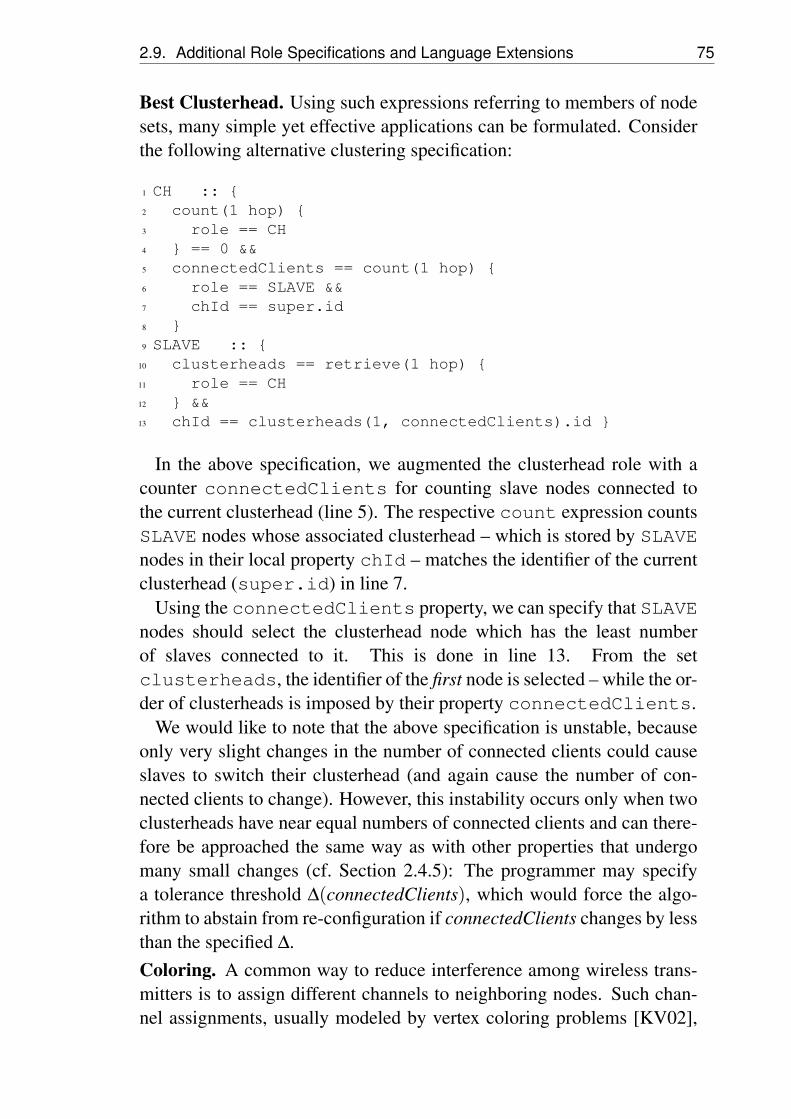
2.9. Additional Role Specifications and Language Extensions 75
Best Clusterhead. Using such expressions referring to members of nodesets, many simple yet effective applications can be formulated. Considerthe following alternative clustering specification:
1 CH :: {2 count(1 hop) {3 role == CH4 } == 0 &&5 connectedClients == count(1 hop) {6 role == SLAVE &&7 chId == super.id8 }9 SLAVE :: {
10 clusterheads == retrieve(1 hop) {11 role == CH12 } &&13 chId == clusterheads(1, connectedClients).id }
In the above specification, we augmented the clusterhead role with acounter connectedClients for counting slave nodes connected tothe current clusterhead (line 5). The respective count expression countsSLAVE nodes whose associated clusterhead – which is stored by SLAVEnodes in their local property chId – matches the identifier of the currentclusterhead (super.id) in line 7.
Using the connectedClients property, we can specify that SLAVEnodes should select the clusterhead node which has the least numberof slaves connected to it. This is done in line 13. From the setclusterheads, the identifier of the first node is selected – while the or-der of clusterheads is imposed by their property connectedClients.
We would like to note that the above specification is unstable, becauseonly very slight changes in the number of connected clients could causeslaves to switch their clusterhead (and again cause the number of con-nected clients to change). However, this instability occurs only when twoclusterheads have near equal numbers of connected clients and can there-fore be approached the same way as with other properties that undergomany small changes (cf. Section 2.4.5): The programmer may specifya tolerance threshold ∆(connectedClients), which would force the algo-rithm to abstain from re-configuration if connectedClients changes by lessthan the specified ∆.Coloring. A common way to reduce interference among wireless trans-mitters is to assign different channels to neighboring nodes. Such chan-nel assignments, usually modeled by vertex coloring problems [KV02],
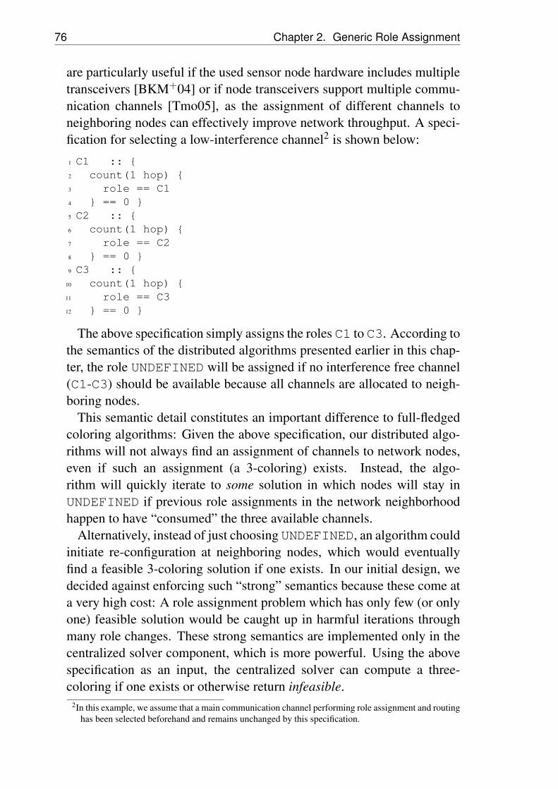
76 Chapter 2. Generic Role Assignment
are particularly useful if the used sensor node hardware includes multipletransceivers [BKM+04] or if node transceivers support multiple commu-nication channels [Tmo05], as the assignment of different channels toneighboring nodes can effectively improve network throughput. A speci-fication for selecting a low-interference channel2 is shown below:
1 C1 :: {2 count(1 hop) {3 role == C14 } == 0 }5 C2 :: {6 count(1 hop) {7 role == C28 } == 0 }9 C3 :: {
10 count(1 hop) {11 role == C312 } == 0 }
The above specification simply assigns the roles C1 to C3. According tothe semantics of the distributed algorithms presented earlier in this chap-ter, the role UNDEFINED will be assigned if no interference free channel(C1-C3) should be available because all channels are allocated to neigh-boring nodes.
This semantic detail constitutes an important difference to full-fledgedcoloring algorithms: Given the above specification, our distributed algo-rithms will not always find an assignment of channels to network nodes,even if such an assignment (a 3-coloring) exists. Instead, the algo-rithm will quickly iterate to some solution in which nodes will stay inUNDEFINED if previous role assignments in the network neighborhoodhappen to have “consumed” the three available channels.
Alternatively, instead of just choosing UNDEFINED, an algorithm couldinitiate re-configuration at neighboring nodes, which would eventuallyfind a feasible 3-coloring solution if one exists. In our initial design, wedecided against enforcing such “strong” semantics because these come ata very high cost: A role assignment problem which has only few (or onlyone) feasible solution would be caught up in harmful iterations throughmany role changes. These strong semantics are implemented only in thecentralized solver component, which is more powerful. Using the abovespecification as an input, the centralized solver can compute a three-coloring if one exists or otherwise return infeasible.
2In this example, we assume that a main communication channel performing role assignment and routinghas been selected beforehand and remains unchanged by this specification.

2.9. Additional Role Specifications and Language Extensions 77
In contrast, having nodes locally revert to UNDEFINED if no other roleis feasible, removes a large amount of the interdependence between neigh-boring nodes and allows the algorithms to converge quickly. Moreover,these “weaker” semantics are quite useful. For example, in sparse net-works in which many feasible role assignments according to the abovespecification exist, the distributed algorithm will very quickly converge toone of them – or to a solution in which only very few nodes remain withUNDEFINED. Moreover, the application developer may provide customcode for nodes in the UNDEFINED role, i.e., which lets the node sleepuntil a channel becomes available.
We close this section with an example specification of the above prob-lem for a larger number of channels:
1 CHANNEL-ASSIGNED :: {2 neighbors == retrieve(1 hop) {3 role == CHANNEL-ASSIGNED4 } &&5 channel ==6 draw-from {1..MAX-CHANNEL} \ neighbors.channel7 }8 UNDEFINED :: else
The above specification demonstrates a few syntactic features, whichcan be used to render the existing role assignment system more flexible.These features, as above, can be mapped onto local (possibly custom-implemented) library functions or to more powerful operators provided bythe local node’s runtime. In this example, the function draw-from(S)chooses a random element from a given set S, or evaluates to false if S= /0.
The operation {1..n} constructs a set consisting of the values 1through n. If a local property P is of type node set, the expression P.x canbe used to generate a set of all different node properties x that occurredat nodes in the set P. Note that the expression neighbors.channelis well-defined, as the check for the CHANNEL-ASSIGNED role (line 3),based on short-circuit semantics, ensures that the property channel isset properly at all nodes in neighbors.
The symbol ‘\’ refers to set subtraction. In summary, the expression inlines 5–6 chooses a random channel from the channels not used by nodesin the one-hop neighborhood of the current node.
In the above, we have listed a set of specification examples that shouldunderline the initial claim that role assignment is a generic concept thatcan be useful for a wide range of applications. In some of these specifica-tions, we introduced slight extensions to the specification syntax, which
78 Chapter 2. Generic Role Assignment
we deem worthwhile implementing in future work, as we expect them toprovide for a new set of important applications. All envisioned extensionsinvolve only local operations that could be supported by a more power-ful local runtime environment on the network nodes, while the basic roleassignment protocol (based on repeated property propagation and subse-quent rule evaluation based on a nodes local knowledge) could still beused to support these specifications as well.
2.10 Summary
In this chapter, we have investigated a novel programming abstractioncalled generic role assignment, which automatically assigns roles to sen-sor nodes based on their properties and the properties of their networkneighborhood.
We have presented a distributed algorithm for role assignment and twovariations that perform probabilistic initialization. Through an extensivequantitative evaluation, we have shown that role assignment is not only apowerful tool, but can also be implemented in an efficient and robust way.Further, we described an extension to our role assignment system thatmaps a given role assignment instance – consisting of a network topology,a set of node properties, and a role assignment specification – to an integerlinear program formulation. This extension provides developers with avaluable tool for analyzing the feasibility, optimality, and termination ofrole assignment specifications.
A particularly noteworthy application of generic role assignment israpid prototyping for sensor networks. Currently, the deployment ofsensor networks often involves a trial-and-error phase, where algorithmsand protocols are tested in different configurations in real-world settings(e.g., [WAJR+05]). With generic role assignment, these different config-urations could be easily generated and changed. While all componentsunder test could be loaded onto the nodes before deployment, these couldbe started and stopped through the assignment of certain roles and initial-ize their respective configuration parameters from the property directory.
As we have argued, one desired property of role-based network config-uration is that it obeys certain global optimization criteria, for example,minimizing the number of required on nodes while maintaining coverage.While such optimization can be performed using the provided solver com-ponent, we have not provided such a feature in our distributed algorithms.
2.10. Summary 79
The distributed generic role assignment approach instead focuses onease of use: It has been designed to allow developers to rapidly prototypeconfiguration heuristics whose quality is sufficient. For example, the ab-straction can well express various clustering heuristics. This includes theclustering specifications we presented in this chapter as well as the con-nected dominating set heuristics used by passive clustering [KG02], or amaximum independent set (implemented by our system if one specifiesthat on nodes are not allowed to have on neighbors). A maximal indepen-dent set can be used to approximate the minimum dominating set problemas (in unit disk graphs) it is only a constant factor worse than the optimalconfiguration [Mos07].
Nevertheless, a generic algorithm that computes optimal solutions fora wide-range role-based configuration problems is an intruiging goal.Based on the variety of applications which can be expressed using therole specification language, devising an algorithm that is applicable to allconceivable specifications remains a challenge. As it turns out, however,such an algorithm can be provided for a key subclass of role-based con-figuration problems, as we describe in the next chapter.

80 Chapter 2. Generic Role Assignment

3 Distributed Facility Location
In an important subclass of role-based configuration problems, a set ofnetwork nodes must be chosen to provide a service to their networkneighborhood. Many application examples we have discussed in the pre-vious chapter belong to this class, such as clustering [BMP04], wherecluster heads serve as communication hubs for nearby nodes, or ag-gregator placement [MFHH02], where some nodes collect and aggre-gate sensor data from nearby sensor nodes. Recently, tiered sensor net-works [GGJ+06] have been proposed, consisting of resource-poor sensornodes in the first tier and powerful hub nodes in the second tier. In thesenetworks, every sensor node is assigned to and controlled by a hub node.Note that in all of the above examples, configuration consists in electingsome nodes as servers while the remaining client nodes are assigned to aserver.
While, next to generic role assignment, many specialized proposals ex-ist for finding such network configurations, these approaches often do notpay attention to optimizing the overall cost of these configurations, whichconsists of two components: on the one hand, the costs of operating theservers (e.g., representing the servers’ increased communication load asthese forward traffic for many clients), and, on the other hand, the costsof communication between clients and their server. In wireless networks,the latter cost can be dependent on the physical distance between a clientand its server (as a longer wireless link requires higher transmit power andthus increased energy consumption), on the number of hops in a multi-hopnetwork graph, or on interference and network congestion. In all cases,lowering communication costs by means of additional server nodes mayprove beneficial.
The goal of this chapter is to provide a generic and practical mecha-nism for finding cost-optimized solutions to the above self-configurationproblems. Our approach is based on the observation that the above opti-mization problem can be modeled as an (uncapacitated) facility locationproblem [Vyg05, Vaz03]. There, we are given a set F of facilities, aset C of clients (also known as cities or customers), a cost fi for open-

82 Chapter 3. Distributed Facility Location
ing a facility i ∈ F and connection costs ci j for connecting client j tofacility i. The objective is to open a subset of facilities in F and con-nect each client to an open facility such that the sum of connection andopening costs is minimized. Open facilities represent server nodes whichcan be used to provide a particular service to network neighbors (just likeclusterhead nodes in the previous chapter). The remaining clientnodes correspond to nodes assigned the role slave.
Although the facility location problem has been studied extensively inthe past, no practical solutions exist that would be suitable for multi-hopsensor networks. While distributed algorithms for facility location exist,they are either not generally applicable [GLS06], require a certain (albeitsmall) amount of global knowledge [MW05], require impractical com-munication models [MW05, CEPS05], or (based on the provided approx-imation factor [CEPS05]) might not improve over the heuristic clusteringspecifications we provided in the previous chapter – or over clusteringheuristics from related work.
In this chapter, we therefore contribute a local facility location algo-rithm that lends itself well for implementation in multi-hop sensor net-works, and provides an approximation factor of 1.61 for metric instances(cf. Section 3.1). By means of an experimental study, we show that,for typical problem instances derived from sensor network configurationproblems, the algorithm provides near-optimal solutions and terminatesafter few communication rounds.
While the above view adopts a static graph model of sensor networks,practical sensor networks are rather dynamic: Nodes may fail and thequality of wireless links fluctuates over time. To make our algorithm ap-plicable to such realistic settings, we propose a set of rules to repair asensor network configuration in case of node failures, additions, and linkquality changes. Further, we evaluate our algorithms and the proposeddynamic adaptation rules using link quality traces obtained from an oper-ative sensor network deployment.
Compared with the previous chapter, the provided facility location al-gorithms export a narrower configuration interface to application devel-opers. Instead of role specifications, developers are expected to provide aset of opening and connection cost parameters or, alternatively, a custom-implemented function which allows nodes to compute the respective costparameters locally. In return, the underlying implementation can provideintriguing performance guarantees, which constitute the main motivationof this chapter.
3.1. Model and Applications 83
3.1 Model and Applications
The facility location problem can be used to model configuration deci-sions in multi-hop networks in a variety of ways. As before, we model themulti-hop network subject to configuration as a graph G = (V,E). Typi-cally, a network node takes on the role of a client and that of a potentialfacility at the same time, that is, F = C = V . If a node i ∈ V is selectedas an open facility, it will take on the role of a server. The remainingslave nodes will be associated to a certain server node in their networkneighborhood.
In some cases, only a subset of nodes have the necessary capabilities(e.g., remaining energy, available sensors, communication bandwidth, orprocessing power) that make them eligible as a facility, which results inF ⊆ C = V . The role assignment framework presented in the previousChapter 2 may be used to compute the set of potential facility nodes F .The algorithms of this chapter can then be used to open a subset from thenodes F which serves the network nodes C efficiently.
The respective settings of opening costs fi and connection costs ci j canimplement various applications. In most cases, connection costs ci j ofan existing a network link (i, j) ∈ E represent a link quality metric thatcan be determined locally at the nodes. In the application examples ofthis chapter, we assume that the nodes can control the power they use forsending. Therefore, we set connection costs ci j as proportional to g(i, j)2
where g(i, j) denotes the distance in m between i and j – implementingthe energy-level required to send messages from j to i.
For pairs of nodes (i, j) which cannot directly communicate in the un-derlying network graph, i.e., (i, j) /∈ E, different settings of ci j allow tospecify desired configurations. Setting ci j = ∞ when (i, j) /∈ E would re-quire that every client has a facility as a direct neighbor. We will denotethis problem formulation as one-hop. An example configuration usingsuch parameters is shown in Figure 3.1(a).
Alternatively, the network developer may be interested in allowingnodes to connect to facilities which are an arbitrary number of hops away– as long as the communication costs adequately represent the energyrequired to communicate between i and j. To implement such configu-rations, ci j can be set to the shortest network path between i and j. Therequired shortest-paths computation will be achieved using a local floodaround a given node i. We denote this problem as multi-hop and show anexample configuration in Figure 3.1(b).

84 Chapter 3. Distributed Facility Location
(a) One-hop example, fi = 1 (b) Multi-hop example, fi = 5
(c) Multi-hop example, fi = 2×D(sink, i)
Figure 3.1: Effects of different opening cost parameters; D(sink, i) denotes the shortest-path distance to the sink, which is located in the upper left corner

3.1. Model and Applications 85
Depending on the particular setting of ci j one may obtain instances ofthe facility location problem which are not metric. The definition of ametric instance is that connection costs obey the triangle inequality, whichrequires that for any three nodes i, j,k the direct path is shorter than adetour (ci j ≤ cik + ck j).
If the input to a facility location algorithm is non-metric, the problem isparticularly hard to solve (see Section 3.2 below). Particularly, the one-hop setting results in a non-metric instance because of two reasons: Thefirst is that, for two non-neighboring nodes, the one-hop path is modeledby infinite costs, while a multi-hop path exists. The second is that settingconnection costs proportional to the squared geographic distance betweentwo nodes results in non-metric instances, for example:
i j
k4
8
1
In turn, the multi-hop problem formulation, in which ci j are computedon the fly to correspond to the shortest path between i and j, represents ametric instance of the facility location problem.
Finally, the opening costs provide developers with an additional lever toexpress properties of the configuration they desire. For example, the open-ing costs fi of a node i can represent the communication effort involvedif this node were to become a service provider for its network neighbor-hood. In a network in which open facilities represent clusterheads whichmust keep their receivers on at all times to receive traffic from associ-ated clients, fi can quantify the energy required for operating the node’stransceiver. This is usually a multiple of ci j, the effort involved in a clientnode’s communication with its clusterhead in a given epoch.
Moreover, opening costs fi may take into account the effort involved ifclusterheads were to forward data to the network sink. In Figure 3.1(c),we show an example of a multi-hop configuration in which opening costsfi are proportional to the node i’s network distance to the sink. Suchparameterization is useful if one assumes that clusterheads must performrepeated communication with the sink which, based on aggregation, doesnot increase significantly with the number of connected clients. In thissetting, it is efficient to let facilities that are far from the sink connect moreclients at higher connection costs, as shown in the results of Figure 3.1(c).
In the course of this chapter, we will use the three parameterizationssketched in Figure 3.1 to evaluate a set of distributed facility location al-

86 Chapter 3. Distributed Facility Location
gorithms which can be applied to the above one-hop and multi-hop prob-lem settings.
3.2 Related Work
An ample amount of literature exists on centralized approximation al-gorithms for the NP-hard facility location problem [Vyg05]. Such al-gorithms are not applicable as collecting a global view of the networktopology at a single point (e.g., at the network basestation) represents aprohibitive communication overhead.
For non-metric instances of the facility location problem, even approx-imations are hard to come by: As the set cover problem can be reducedto (non-metric) facility location, the best achievable approximation ra-tio (even with a centralized algorithm) is logarithmic1 in the number ofnodes [Fei98]. A classic and simple algorithm [Hoc82] already comesclose to this lower bound. Distributed approximations are rare: [MW05]solve non-metric facility location even in a constant number of commu-nication rounds. However, the algorithm requires that a coefficient ρ,which is computed from a global view of the problem instance, is dis-tributed to all nodes before algorithm execution – which prevents it frombeing used “as-is” in practice. Moreover, the algorithm requires globalcommunication among all relevant clients and facilities and therefore canonly efficiently be used in the one-hop setting where such communicationcan be implemented efficiently by wireless broadcast. Finally, the bestapproximation factor it can obtain, which is independent of the probleminstance, is on the order of O(log(m+n) log(mn)) where m and n denotethe number of facilities and clients, respectively.
For metric instances of the facility location problem, much betterapproximation factors ∈ O(1) can be achieved. While it has beenshown [GK99] that a polynomial-time algorithm cannot obtain an ap-proximation ratio better than 1.463, a centralized algorithm [MYZ02]already provides a solution that is at most a factor of 1.52 away fromthe optimum. For the metric case, a distributed algorithm has been men-tioned in [CEPS05] which solves a constrained version of the problemin which facilities and clients may be at most 3 hops away. It providesa 3 + ε approximation factor derived from a parallelized execution ofa respective centralized algorithm [JV99] and is formulated in terms of
1This holds unless every problem in NP can be solved in O(nO(log logn)) time.

3.3. Centralized Algorithms 87
a synchronous message passing model. The same paper [CEPS05] in-cludes additional versions, which restrict the facility location problem inone way or another. Only recently, a constrained version of the facil-ity location problem (in which all opening costs are equal) has been ad-dressed in a distributed manner [GLS06]. This algorithm also requires asynchronous message passing model and global communication amongall nodes in each round. Finally, a distributed algorithm based on hill-climbing [KSW05] addresses a version of the problem in which exactlyk facilities are opened. In this approach, the worst-case time complexityand the obtained approximation factor are not discussed explicitly.
In this chapter, we develop a distributed version of a centralized al-gorithm [JMM+03] which provides an 1.61 approximation factor withmetric instances. Compared to related work, our work improves on theapproximation factor achievable in a distributed manner. Moreover, weprovide adaptations for executing this algorithm in multi-hop networksfor which, to our knowledge, no local algorithm with guaranteed worst-case approximation factor exists. Finally, compared to [MW05, CEPS05,GLS06], our algorithms do not require a synchronous message passingmodel. Instead, they perform synchronization among network neighborsimplicitly as nodes wait for incoming messages.
The remainder of this chapter is structured as follows. In Section 3.3,we briefly summarize the centralized algorithms [JMM+03] which pro-vide the foundation for our work. We then describe their distributed re-formulation in two steps. The first version, given in Section 3.4, still re-quires global communication, namely, that all clients communicate withall relevant facilities in each step, and is therefore only applicable to theone-hop setting, where this can be efficiently implemented as a wirelessbroadcast. In the second step, we use this algorithm as a subroutine in thealgorithms of Section 3.5, which distribute messages only to a local neigh-borhood around the sending node and may therefore be used in multi-hopnetworks. Finally, we provide experimental results in Section 3.6 and asummary of the chapter in Section 3.7.
3.3 Centralized Algorithms
Jain et al. [JMM+03] devised two centralized approximation algorithmsfor the facility location problem. Both use the notion of a star (i,B) con-sisting of a facility i and an arbitrary choice of clients B⊆C (in clusteringterminology, a star corresponds to a cluster leader and a set of associated
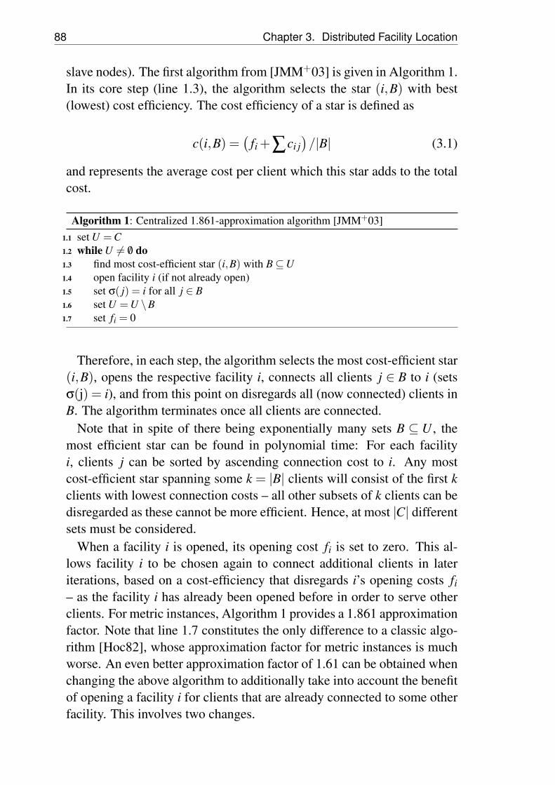
88 Chapter 3. Distributed Facility Location
slave nodes). The first algorithm from [JMM+03] is given in Algorithm 1.In its core step (line 1.3), the algorithm selects the star (i,B) with best(lowest) cost efficiency. The cost efficiency of a star is defined as
c(i,B) =(
fi +∑ci j)/|B| (3.1)
and represents the average cost per client which this star adds to the totalcost.
Algorithm 1: Centralized 1.861-approximation algorithm [JMM+03]set U = C1.1
while U 6= /0 do1.2
find most cost-efficient star (i,B) with B ⊆U1.3
open facility i (if not already open)1.4
set σ( j) = i for all j ∈ B1.5
set U = U \B1.6
set fi = 01.7
Therefore, in each step, the algorithm selects the most cost-efficient star(i,B), opens the respective facility i, connects all clients j ∈ B to i (setsσ(j) = i), and from this point on disregards all (now connected) clients inB. The algorithm terminates once all clients are connected.
Note that in spite of there being exponentially many sets B ⊆ U , themost efficient star can be found in polynomial time: For each facilityi, clients j can be sorted by ascending connection cost to i. Any mostcost-efficient star spanning some k = |B| clients will consist of the first kclients with lowest connection costs – all other subsets of k clients can bedisregarded as these cannot be more efficient. Hence, at most |C| differentsets must be considered.
When a facility i is opened, its opening cost fi is set to zero. This al-lows facility i to be chosen again to connect additional clients in lateriterations, based on a cost-efficiency that disregards i’s opening costs fi– as the facility i has already been opened before in order to serve otherclients. For metric instances, Algorithm 1 provides a 1.861 approximationfactor. Note that line 1.7 constitutes the only difference to a classic algo-rithm [Hoc82], whose approximation factor for metric instances is muchworse. An even better approximation factor of 1.61 can be obtained whenchanging the above algorithm to additionally take into account the benefitof opening a facility i for clients that are already connected to some otherfacility. This involves two changes.

3.4. One-hop Approximation 89
First, this requires that a revised cost-efficiency definition is used inline 1.3. We let B(i) denote the set of clients j which are already con-nected to some facility σ( j) and would benefit if i would be opened astheir connection cost to i would be lower than their current connectioncost cσ( j) j, i.e.,
B(i) ={
j ∈C with σ( j) 6= none and ci j < cσ( j) j}
. (3.2)
The cost efficiency of a star (i,B) can now be restated as
c(i,B) =
(fi + ∑
j∈Bci j− ∑
j∈B(i)(cσ( j) j− ci j)
)/|B|. (3.3)
A second analogous change is made to line 1.5. In addition to the clientswhich are part of the most-efficient star (i,B), all already-connectedclients B(i) which benefit from switching are connected to i. For this,line 1.5 becomes
set σ( j) = i for all j ∈ B∪B(i).
The authors prove in [JMM+03] that this change improves the approx-imation factor to 1.61 for metric instances. In the following, we willpresent a distributed version of this 1.61-algorithm. In the discussed dis-tributed adaptations, we will always use the revised cost-efficiency defi-nition given in equation (3.3).
3.4 One-hop Approximation
Consider the distributed algorithms given in Algorithm 2 (for facilities)and 3 (for clients). We will show below that they perform the exact samesteps as the centralized Algorithm 1. While these algorithms require thateach client communicates with each facility and vice versa, the algorithmscan be also applied “locally” such that each node communicates only withits network neighbors. This way, they can be used to compute a solution tothe one-hop version of the facility location problem, for example, to com-pute an energy-efficient clustering that takes the costs of individual linksinto account. Unfortunately, this constrained problem version results in anon-metric instance (see Section 3.1) and thus the approximation guaran-tee of 1.61 cannot be preserved. However, in the next section, we will usethese algorithms as a subroutine to obtain an algorithm that maintains theapproximation factor of 1.61 for multi-hop sensor networks. Moreover,
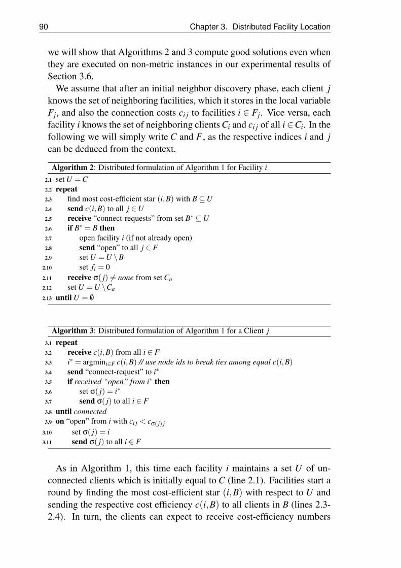
90 Chapter 3. Distributed Facility Location
we will show that Algorithms 2 and 3 compute good solutions even whenthey are executed on non-metric instances in our experimental results ofSection 3.6.
We assume that after an initial neighbor discovery phase, each client jknows the set of neighboring facilities, which it stores in the local variableFj, and also the connection costs ci j to facilities i ∈ Fj. Vice versa, eachfacility i knows the set of neighboring clients Ci and ci j of all i∈Ci. In thefollowing we will simply write C and F , as the respective indices i and jcan be deduced from the context.
Algorithm 2: Distributed formulation of Algorithm 1 for Facility iset U = C2.1
repeat2.2
find most cost-efficient star (i,B) with B ⊆U2.3
send c(i,B) to all j ∈U2.4
receive “connect-requests” from set B∗ ⊆U2.5
if B∗ = B then2.6
open facility i (if not already open)2.7
send “open” to all j ∈ F2.8
set U = U \B2.9
set fi = 02.10
receive σ( j) 6= none from set Ca2.11
set U = U \Ca2.12
until U = /02.13
Algorithm 3: Distributed formulation of Algorithm 1 for a Client jrepeat3.1
receive c(i,B) from all i ∈ F3.2
i∗ = argmini∈F c(i,B) // use node ids to break ties among equal c(i,B)3.3
send “connect-request” to i∗3.4
if received “open” from i∗ then3.5
set σ( j) = i∗3.6
send σ( j) to all i ∈ F3.7
until connected3.8
on “open” from i with ci j < cσ( j) j3.9
set σ( j) = i3.10
send σ( j) to all i ∈ F3.11
As in Algorithm 1, this time each facility i maintains a set U of un-connected clients which is initially equal to C (line 2.1). Facilities start around by finding the most cost-efficient star (i,B) with respect to U andsending the respective cost efficiency c(i,B) to all clients in B (lines 2.3-2.4). In turn, the clients can expect to receive cost-efficiency numbers

3.4. One-hop Approximation 91
c(i,B) from all facilities i ∈ F (line 3.2). In order to connect the mostcost-efficient star among the many existing ones, clients reply to the facil-ity i∗ that has sent the lowest c(i∗,B) with a “connect request” (line 3.4).In turn, facilities collect a set of clients B∗ which have sent these “con-nect requests” (line 2.5). Intuitively, a facility should only be opened ifB = B∗, that is, if it has connect requests from all clients B in its most effi-cient star (line 2.6). This is necessary, as it could happen that some clientsin B have decided to connect to a different facility than i as this facilityspans a more cost efficient star. So, if all clients in B are ready to connect,facility i opens, notifies all clients in B about this, removes the connectedclients B from U , and sets its opening costs to 0 (lines 2.7-2.10) as in thecentralized algorithm.
If a client j receives such an “open” message from the same facility i∗
which it had previously selected as the most cost efficient, it can connectto i∗ (lines 3.5-3.6). Further, in line 3.7, client j notifies all facilities thatit is now connected to i∗, which update their sets of unconnected clientsU in lines 2.11-2.12.
Once connected, clients simply switch the facility they are connectedto in case a closer facility becomes available (lines 3.9-3.10). This fea-ture enables the 1.61 approximation factor. Note that whenever a clientchanges its facility σ( j), it informs all facilities about this (lines 3.7 and3.11). All these σ( j) messages include the associated connection costscσ( j) j and will be received in line 2.11 of the facility algorithm. By thenext iteration, facilities will have received σ( j) and cσ( j) j from all rel-evant clients, and will therefore be able to correctly compute the mostcost-efficient star (line 2.3) according to Eq.(3.3).Discussion. In the following, we argue that the distributed and the cen-tralized versions are equivalent. For this, we denote one execution of theinner loops at Algorithms 3 and 4 as a round. Note that the distributedversion opens some stars out-of-order, that is, earlier than the centralizedversion. The following lemma states that these stars are disjoint from anystar that might follow and has lower cost-efficiency.
Lemma 3.4.1 Let Uk be the set of uncovered clients prior to the begin-ning of round k. If a client j is part of a star (i,B) opened by the dis-tributed algorithm in round k, then there is no star (i′,B′) consideringB′ ⊆Uk with j ∈ B′ and c(i′,B′) < c(i,B).
Proof Assume the contrary, namely that a star (i′,B′) exists withc(i′,B′) < c(i,B) and say j is a client in B′∩B. Note that B′ ⊆Uk, and

92 Chapter 3. Distributed Facility Location
therefore i′ will choose some star (i′,B′′) with cost-efficiency c(i′,B′′) ≤c(i′,B′) in line 2.3. However, as (i,B) is opened in round k, client j hassent its connect request to i and not to i′, which implies c(i′,B′)≥ c(i,B)and contradicts the assumption.
Given the above, we can show that the stars opened by the distributedalgorithm can be re-ordered to correspond to the execution of the central-ized algorithm.
Theorem 3.4.2 The distributed and centralized versions are equivalent.
Proof We sequentialize the distributed algorithm as follows: In the se-quentialized version we open only one star (the globally most cost-efficient star) per round. Further, we postpone opening a star (i,B) whichhas been opened in parallel by the distributed algorithm to a later roundprior to which all stars (i′,B′) with c(i′,B′) < c(i,B) have been processed.Let (i′,B′) denote one such star. Because of Lemma 3.4.1, B′ ∩B = /0,and therefore opening (i′,B′) ahead of time does not remove any client inB from U and therefore does not interfere with opening (i,B). Similarly,postponing any (i,B) will not allow that a more cost-efficient star includ-ing elements of B is formed earlier – again by Lemma 3.4.1. Postponing(i,B) can further influence (raise) the cost-efficiency of the stars (i′,B′) asit changes the set B(i) for these facilities and thus may change the orderin which these are processed. However, as by Lemma 3.4.1 all these starsare mutually disjoint, the order in which they are opened does not affecttotal costs. Finally, all stars opened in parallel are disjoint and re-orderingthem does not change algorithm execution.
Therefore, the sequentialized version opens the same stars as the dis-tributed algorithm. Moreover, as the sequentialized version opens themost cost-efficient star in every round, it implements the execution ofthe centralized algorithm.
Algorithms 2 and 3 therefore provide an approximation factor of 1.61.While the quality of the obtained solutions is intruiging, the worst-casenumber of rounds required by Algorithms 2 and 3 is linear in the numberof nodes, because there can be a unique point of activity around the glob-ally most cost-efficient facility i∗ in each round: Consider for instance achain of m facilities located on a line, where each pair of facilities is inter-connected by at least one client, and assume that facilities in the chainhave monotonously decreasing cost efficiencies. Each client situated be-tween two facilities will send a “connect-request” to only one of them (the

3.5. Multi-hop Approximation 93
more cost efficient), thus the second cannot open. In this example, onlythe facility at the end of the chain can be opened in one round. Similarly,once at least one facility is open, it could happen that in each round onlyone client connects to this facility. The worst-case runtime is thereforeO(n), in which n is the number of network nodes.
The linear number of rounds required by every node in the worst-casewould constitute a high overhead in large networks. However, a worst-case configuration on a larger scale is highly improbable. We will evaluatethe number of rounds required on typical instances derived from sensornetworks in Section 3.6.
As we mentioned, the above algorithm only achieves an 1.61 approxi-mation factor with metric instances. As the metric property implies thata graph must be complete, executing the above algorithms on metric in-stances implies global communication between all clients and facilities.Global communication can only be implemented efficiently in scenarioswhere all nodes are in wireless range of each other.
In our evaluation of Section 3.6, however, we will show that the abovealgorithms perform well even with non-metric one-hop instances. More-over, below we will use the above algorithms as subroutines in an adapted“local” version that functions properly in multi-hop networks.
3.5 Multi-hop Approximation
The described algorithm can be changed to work in multi-hop settings us-ing only a slight adaptation. As it turns out, if connection costs representshortest paths between network nodes, the communication performed bythe algorithms can be restricted to small network neighborhoods. Specif-ically, if one is interested in determining whether a facility i has a cost-efficiency of less than a certain threshold s, it is sufficient to consideronly clients j that are reachable by i over a path with costs of at most s,i.e., clients j with ci j ≤ s. To see this, consider the definition of a facil-ity’s cost-efficiency and assume that some star’s cost efficiency c(i,B)≤ s.One can always obtain an even smaller cost-efficiency once one removesthe clients j ∈ B′ which have ci j > s, that is, c(i,B\B′) < c(i,B).
Similarly, for any facility i, the clients j with cσ( j) j > ci j will not benefitfrom switching to i. Consequently, these clients will not occur in the setB(i) of Eq. (3.3). Therefore, it is sufficient that clients j which becomeconnected to σ( j) distribute σ( j) only to facilities i with cost ci j < cσ( j) j.

94 Chapter 3. Distributed Facility Location
Algorithm 4: Multi-Hop Adaptation of Algorithm 3 for a Client jset s = 1, set σ( j) = none4.1
repeat4.2
set s = s×a4.3
send “start(s)” to all i ∈ Fs4.4
if no “begin(s)” received then continue4.5
repeat4.6
receive c(i,B) from all facilities Fs4.7
set Fa = {i ∈ Fs with c(i,B)≤ s}4.8
if Fa 6= /0 then4.9
i∗ = argmini∈Fa c(i,B) // use node ids to break ties4.10
send “connect-request” to i∗4.11
if received “open(s)” from i∗ then4.12
set σ( j) = i∗4.13
send σ( j) to all i ∈ Fs4.14
until connected or Fa = /04.15
until connected4.16
on “open(s∗)” from i with ci j < cσ( j) j4.17
set σ( j) = i4.18
send σ( j) to all i ∈ Fs∗4.19
In an outer loop added around Algorithms 2 and 3, we therefore ex-ponentially increase the communication scope s, that is, the maximumdistance over which messages are forwarded. Specifically, given a certainscope s, a message is only flooded within a localized neighborhood Ns(i)around the sending node i, where Ns(i) := { j ∈V with ci j ≤ s}. Note thatif the direct link (i, j) is not present in the network graph, ci j representingthe shortest path from j to i can be determined on the fly while flooding amessage within Ns( j). Nodes simply stop forwarding a message if it hascovered a distance larger than s or if it has already been received over ashorter path.
The updated versions are given in Algorithm 4 (clients) and Algorithm 5(facilities). In the following, we will respectively use Cs and Fs to refer toclient and facility nodes within scope s of the current node.
In the outer loop, the considered scope s is raised exponentially(lines 4.3 and 5.3) by a constant a. To initialize an outer round, clients,which have not yet been connected, send a “start” message containingtheir current scope s to all facilities in scope (line 4.4). In turn, facilitieswait for at least one such “start” message for a certain time (line 5.4) uponwhich they reply “begin(s)”. The waiting period must be long enoughto allow relevant clients to send the respective start messages and finishearlier rounds. If no “start” messages were received, facilities simply ad-vance to the next outer round (line 5.4) to wait for “start” messages from

3.5. Multi-hop Approximation 95
Algorithm 5: Multi-Hop Adaptation of Algorithm 2 for Facility iset s = 15.1
repeat5.2
set s = s×a5.3
if “start(s)” received then send “begin(s)” to all j ∈Cs else continue5.4
query σ( j) from all j ∈Cs5.5
set Us = { j ∈Cs with σ( j) = none}5.6
repeat5.7
find most cost-efficient star (i,B) with B ⊆Us5.8
send c(i,B) to all j ∈Us5.9
if c(i,B)≤ s then5.10
receive “connect-requests” from set B∗ ⊆Us.5.11
if B∗ = B then5.12
open facility i (if not already open)5.13
send “open(s)” to all j ∈C5.14
set Us = Us \B, set fi = 05.15
receive σ( j) 6= none from some clients B′ ⊆Us5.16
set Us = Us \B′5.17
until Us = /0 or c(i,B) > s5.18
until s > smax5.19
a larger scope. Clients, analogously, wait and then skip the current roundif no neighboring facility has sent “begin”.
A start message sent by a client j thus triggers execution of one outerround at all the facilities in scope Fs. Facilities then query all clients inscope for their status σ( j) in line 5.5 and compute the set of yet uncon-nected clients Us. This query-reply cycle allows the facility to wait forall relevant clients to catch up to the current scope s. Clients reply to thisquery once they have reached scope s – note that we have omitted therespective code in the client algorithm. Similarly clients can wait for fa-cilities lagging behind in line 4.7 where they expect to receive a messagefrom all facilities in scope.
After this initialization, facilities execute Algorithm 2 in an inner loop(lines 5.7-5.18) and clients react accordingly (lines 4.6-4.15) implement-ing Algorithm 3. Compared to Algorithms 2 and 3, the termination con-ditions of the inner loops must be changed to allow clients and facilitiesto proceed to a larger scope in a properly synchronized manner. As withthe 1-hop version, clients terminate their inner loop once they are con-nected (line 4.15) and facilities once no active clients remain in scope(line 5.18). In addition, within an inner-loop with scope s, the algorithmshould only consider stars (i,B) with cost-efficiency c(i,B) < s. There-fore, facilities only proceed with the current inner loop as long as they areefficient enough for this scope (lines 5.10 and 5.18) while in turn clients
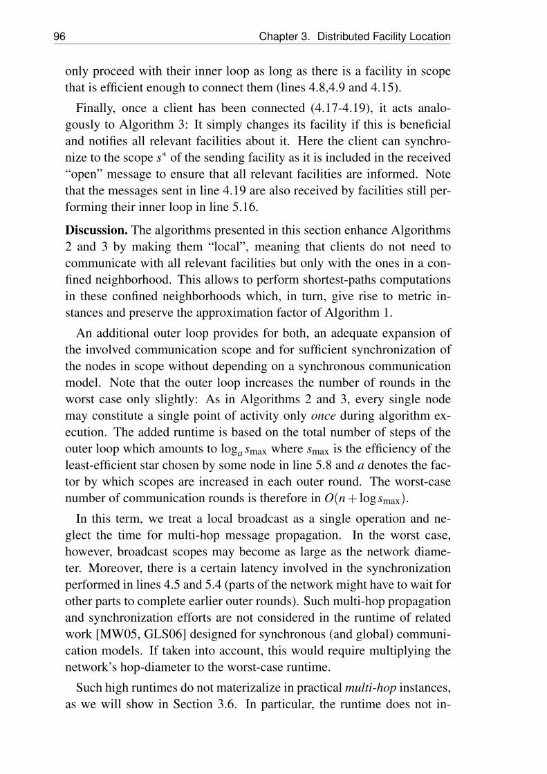
96 Chapter 3. Distributed Facility Location
only proceed with their inner loop as long as there is a facility in scopethat is efficient enough to connect them (lines 4.8,4.9 and 4.15).
Finally, once a client has been connected (4.17-4.19), it acts analo-gously to Algorithm 3: It simply changes its facility if this is beneficialand notifies all relevant facilities about it. Here the client can synchro-nize to the scope s∗ of the sending facility as it is included in the received“open” message to ensure that all relevant facilities are informed. Notethat the messages sent in line 4.19 are also received by facilities still per-forming their inner loop in line 5.16.
Discussion. The algorithms presented in this section enhance Algorithms2 and 3 by making them “local”, meaning that clients do not need tocommunicate with all relevant facilities but only with the ones in a con-fined neighborhood. This allows to perform shortest-paths computationsin these confined neighborhoods which, in turn, give rise to metric in-stances and preserve the approximation factor of Algorithm 1.
An additional outer loop provides for both, an adequate expansion ofthe involved communication scope and for sufficient synchronization ofthe nodes in scope without depending on a synchronous communicationmodel. Note that the outer loop increases the number of rounds in theworst case only slightly: As in Algorithms 2 and 3, every single nodemay constitute a single point of activity only once during algorithm ex-ecution. The added runtime is based on the total number of steps of theouter loop which amounts to loga smax where smax is the efficiency of theleast-efficient star chosen by some node in line 5.8 and a denotes the fac-tor by which scopes are increased in each outer round. The worst-casenumber of communication rounds is therefore in O(n+ logsmax).
In this term, we treat a local broadcast as a single operation and ne-glect the time for multi-hop message propagation. In the worst case,however, broadcast scopes may become as large as the network diame-ter. Moreover, there is a certain latency involved in the synchronizationperformed in lines 4.5 and 5.4 (parts of the network might have to wait forother parts to complete earlier outer rounds). Such multi-hop propagationand synchronization efforts are not considered in the runtime of relatedwork [MW05, GLS06] designed for synchronous (and global) communi-cation models. If taken into account, this would require multiplying thenetwork’s hop-diameter to the worst-case runtime.
Such high runtimes do not materizalize in practical multi-hop instances,as we will show in Section 3.6. In particular, the runtime does not in-

3.6. Evaluation 97
crease with the network size and the involved communication scopes (de-termined by smax) are fairly small compared to the network diameter2.Dynamic Re-configuration. In real-world deployments of sensor net-works, link qualities change over time and nodes may fail. To accom-modate for major changes in the network topology, the algorithms arere-executed at regular intervals. As such re-starts involve relatively highoverhead, these are performed only infrequently (e.g., once a day). In be-tween such re-starts, a client j combines periodic re-evaluations of linkcosts ci j (within a local scope of size cσ( j) j) with a liveness check on thefacility σ( j). In both cases, if σ( j) has failed or a closer open facility hasbeen found, client j re-connects to the closest open facility. In the nextsection, we will show that such adaptations suffice to maintain a close-to-optimal configuration over longer periods of time.
3.6 Evaluation
In the following we present results from two distinct sets of experiments.The first, detailed in Section 3.6.1, is based on simulations which testthe scalability of the proposed algorithms. The second, detailed in Sec-tion 3.6.2, tests the applicability of the proposed algorithms to operationalnetworks with dynamic links.
3.6.1 Scalability
In the experiments based on simulations, we uniformly deployed a vari-able number of nodes onto a 300 m by 300 m area. The network graphhas an edge (i, j) ∈ E if nodes i and j are less than 30 m apart. Assumingthat nodes can control their transmit power, for (i, j) ∈ E we set the con-nection costs ci j to g(i, j)2, in which g(i, j) denotes the distance in metersbetween i and j, and normalize them such that ci j ∈ [0,1].Scenarios. To test our algorithms with a range of applications, we ex-amined three different parameterizations of the problem, of which quali-tative results were shown earlier in Figure 3.1. In the first, shown in Fig-ure 3.1(a), we set opening costs fi = 1 and additionally require that clientsand facilities must be neighbors. We tested the one-hop Algorithms 2 and3 on such instances.
2In fact, smax depends on the application and is proportional to the hardness of the specified configurationproblem: If the desired configuration is inherently non-local, for example, if high opening cost settingsrequire the algorithms to choose only one facility that serves the whole network, smax will be high.

98 Chapter 3. Distributed Facility Location
Further, we tested the multi-hop Algorithms 4 and 5 in two differentsettings, which were also already introduced in Figures 3.1(b) and 3.1(c),respectively. In the first, we set fi = 5 to denote that a high effort isrequired to operate a cluster leader. In the second scenario, we assumedthat cluster leaders must send much data to the network base station andtherefore their operation costs increase with their network distance to thesink (yielding smaller stars close to the sink and larger ones further away).One-Hop Clusters. In the one-hop setting (Figure 3.1(a)), we evaluatedthe costs of configurations produced by different algorithms while varyingthe number of nodes in the simulation area (that is, the node density). Theresults are given in Figure 3.2(a) which shows the costs obtained with thefollowing five methods.
One-hop denotes the simple one-hop algorithms of Section 3.4. Respec-tively, one-hop IP refers to the optimal configuration of the constrainedcase which requires clients to connect to facilities which are direct net-work neighbors. Further, multi-hop denotes the multi-hop algorithm de-scribed in Section 3.5, which has a 1.61 approximation guarantee. Here,clients may connect to facilities which are an arbitrary number of hopsaway. Respectively, multi-hop IP computes the optimal solution to thefacility location problem, in which facilities and clients may be multiplehops apart and the instance is made metric by a centralized shortest-pathscomputation. Finally, MDS IP denotes the optimal solution to the mini-mum dominating set problem, in which dominator nodes represent openfacilities and slave nodes are clients that connect to the closest dominatornode. The costs are computed using the original (non-metric) instance.
The costs of a minimum dominating set (MDS IP) which suffer fromexpensive long links mark one end of the optimization spectrum. Herewe argued that facility location can provide a more energy efficient con-figuration as it takes costs of the links between clients and servers intoaccount. On the other hand, the optimal facility-location based configura-tion (multi-hop IP) marks the other end of the spectrum as it represents alower bound for the employed approximation algorithms.
The one-hop algorithm performs well and is even close to the respec-tive optimal configuration one-hop IP, although it operates on non-metricinstances and thus without a guaranteed approximation factor.
Note that in this particular setting, the constrained versions, which re-quire facilities and clients to be direct neighbors (one-hop and the optimalone-hop IP), are not far away from the multi-hop results and the optimumof the unconstrained case (multi-hop IP). This is due to the low opening
3.6. Evaluation 99
80
100
120
140
160
180
200
220
240
260
200 250 300 350 400 450 500
Cos
ts
Number of nodes
one-hopone-hop IP
multi-hopmulti-hop IP
MDS IP
(a) One-hop
180
200
220
240
260
280
300
320
340
200 250 300 350 400 450 500
Cos
ts
Number of nodes
distdist IPsimple
simple IP
(b) Multi-hop
Figure 3.2: Performance of one-hop and multi-hop algorithms
100 Chapter 3. Distributed Facility Location
costs we used, which are set to fi = 1 for all facilities. With larger openingcosts, multi-hop solutions would benefit more from larger stars.
Multi-Hop Clusters. In the experiments shown in Figure 3.2(b), weadditionally evaluate the quality of the solutions obtained by the multi-hop algorithm with the two different opening cost settings shown in Fig-ures 3.1(b) and 3.1(c). In the first (denoted as simple) we set opening coststo a constant fi = 5 which corresponds to configurations as shown in Fig-ure 3.1(b). In the second, denoted as dist, we apply the heuristic shownin Figure 3.1(c), where the opening costs correspond to twice the costs ofthe shortest path to the sink. In both cases, the results of the distributedimplementation are very close to the achievable optimum computed byCPLEX on the same instance.
Runtime and Overhead. In the experiments shown in Figure 3.2(b), thescope s started out with 0.2 and a was set to 2, thus doubling the scopein each outer round. Note, however, that these two parameters do notinfluence the quality of the obtained solution. Rather, they determine thetrade-off achieved between the runtime of the algorithms and the scopewithin which messages are sent. On the one hand, the smaller a is set, theless likely it is that scopes are increased by too much (in vain). On theother hand, lower values of a increase the number of outer rounds3.
Figure 3.3 demonstrates this trade-off as observed in the simulation runcorresponding to Figure 3.2(b). In Figure 3.3(a) we show the averagescope with which messages were sent during algorithm execution, givendifferent settings of a (the scope s always starts at 0.2). The lower weset a, the better the results as the scope is increased by smaller amounts.Note that in general, the effort involved in the execution of our algorithmis proportional to the “locality” implied by the problem instance: On theone hand, if opening costs are high (here fi = 5), a facility will generallyconnect clients in a larger neighborhood (as seen in Figure 3.1(b)). Onthe other hand, the experienced scopes are even much lower with smallopening costs (e.g., for fi = 1, not shown).
In contrast, in Figure 3.3(b), we show the runtime in rounds (one roundcorresponds to one iteration of the inner loop) of the multi-hop algorithmon the same instances. Note that, while previously the error bars indicatedconfidence intervals of 95%, we use them in Figure 3.3(b) to mark themaximum and minimum values that occurred in 10 random instances (as
3Interstingly, our experiments show that the average number of communication rounds, whose worstcase amounts to O(n + loga smax), is in fact dominated by the latter term loga smax. The case wheresingle nodes slow down algorithm execution (giving rise to the first term n) is highly unlikely.

3.6. Evaluation 101
0.5
1
1.5
2
2.5
3
200 250 300 350 400 450 500
Ave
rage
sco
pe s
ize
Number of nodes
a=2.0a=1.5a=1.2a=1.1
(a) Scope
10
15
20
25
30
35
40
45
50
55
200 250 300 350 400 450 500
Run
time
(in r
ound
s)
Number of nodes
a=2.0a=1.5a=1.2a=1.1
(b) Rounds
Figure 3.3: Average scope size vs. total runtime (in rounds). In Figure 3.3(b) the errorbars denote the maximum and the minimum that occurred.
102 Chapter 3. Distributed Facility Location
we are particularly interested in the maximum value). The results showthat – while in theory the worst case runtime can be large – in typicalinstances based on multi-hop networks the runtime is sufficiently smalland does not even grow with the number of nodes. Moreover, based onthe trade-off between runtime and scope size, the runtime improves withhigher a values. Finally, the scope size decreases with increasing net-work density. This is due to the fact that, given certain opening costs, thealgorithms will connect stars of around the same size (namely, facilitiesare opened once enough clients are connected to pay for opening them).Therefore, smaller stars are opened in denser networks and the cumulatedcommunication overhead stays the same.
3.6.2 Network Dynamics
One open question is whether such, albeit close-to-optimal solutions, canprovide a benefit for real-world deployments in which the network topol-ogy changes over time. To obtain realistic link qualities, we extended atestbed of 13 TMote Sky modules that gather temperature, humidity, andlight measurements from our office premises to record network topologyinformation as well. In addition to its sensor measurements, every 5 sec-onds, a node reports the set of nodes from which an application-layermessage has been received since the last update.
Such topology information received from each node i allows to computea (packet-level) link quality estimate ei j(t) for each network link directedfrom j to i [WTC03]. The estimate ei j(t) is based on the packet successrate ri j = packets received in T
packets expected in T which is smoothened using an exponentiallyweighted moving average such that ei j(t) = αri j(t) + (1−α)ei j(t − 1).In our experiments, we set α=0.6 according to [WTC03] and T to 300 s.We transform the quality estimates ei j ∈ [0,1] into link cost estimates bysetting ci j = 1 + 10(1− ei j) if ei j > 0.5 and ci j = ∞, otherwise. Further,we set opening costs to constant fi = 2.
To give the reader an impression of the examined networks, Figure 3.4shows our sensor node deployment, the resulting network topology, and aconfiguration computed by the multi-hop algorithms.
Given the link costs {ci j(t0)} observed at a certain time of the exper-iment t0, we let the presented multi-hop algorithms compute a configu-ration (a set of open facilities and assigned clients), whose costs C(t0, t)vary with t as link qualities change over time. Once a configuration has
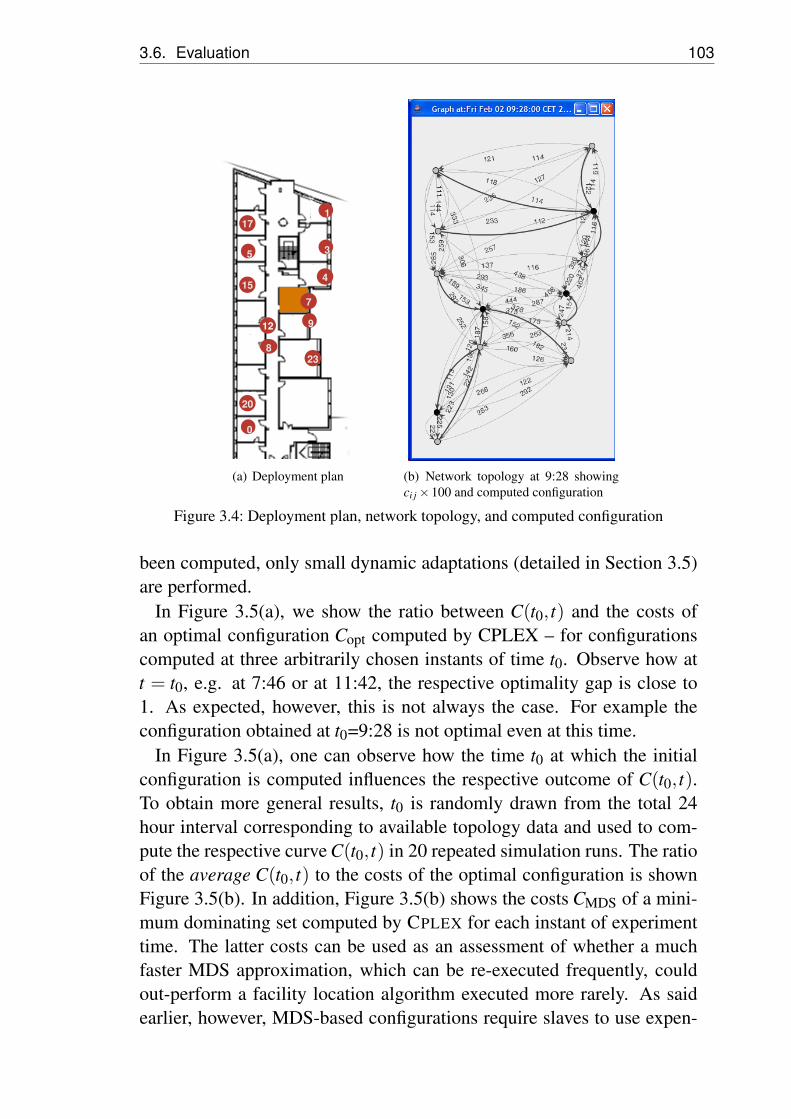
3.6. Evaluation 103
8
1
53
9
20
15
0
23
7
4
17
12
(a) Deployment plan (b) Network topology at 9:28 showingci j ×100 and computed configuration
Figure 3.4: Deployment plan, network topology, and computed configuration
been computed, only small dynamic adaptations (detailed in Section 3.5)are performed.
In Figure 3.5(a), we show the ratio between C(t0, t) and the costs ofan optimal configuration Copt computed by CPLEX – for configurationscomputed at three arbitrarily chosen instants of time t0. Observe how att = t0, e.g. at 7:46 or at 11:42, the respective optimality gap is close to1. As expected, however, this is not always the case. For example theconfiguration obtained at t0=9:28 is not optimal even at this time.
In Figure 3.5(a), one can observe how the time t0 at which the initialconfiguration is computed influences the respective outcome of C(t0, t).To obtain more general results, t0 is randomly drawn from the total 24hour interval corresponding to available topology data and used to com-pute the respective curve C(t0, t) in 20 repeated simulation runs. The ratioof the average C(t0, t) to the costs of the optimal configuration is shownFigure 3.5(b). In addition, Figure 3.5(b) shows the costs CMDS of a mini-mum dominating set computed by CPLEX for each instant of experimenttime. The latter costs can be used as an assessment of whether a muchfaster MDS approximation, which can be re-executed frequently, couldout-perform a facility location algorithm executed more rarely. As saidearlier, however, MDS-based configurations require slaves to use expen-

104 Chapter 3. Distributed Facility Location
1
1.05
1.1
1.15
1.2
1.25
1.30
7:0
0
07
:30
08
:00
08
:30
09
:00
09
:30
10
:00
10
:30
11
:00
11
:30
12
:00
Op
tim
alit
y g
ap
t
7:46
9:28
11:42
(a) C(t0, t)/Copt for different t0 during 5 hours
1
1.2
1.4
1.6
1.8
2
18
:00
20
:00
22
:00
00
:00
02
:00
04
:00
06
:00
08
:00
10
:00
12
:00
14
:00
16
:00
18
:00
Op
tim
alit
y g
ap
t
CMDS / Copt
Average C(t0,t) / Copt
Confidence intervals (95%)
(b) Average C(t0, t)/Copt vs. MDS during 24 hours
Figure 3.5: Solutions’ optimality over time
3.7. Summary 105
sive links (with poor link quality estimates) to communicate with theircluster leader. Such “bad” links are often the most volatile and causethe costs of an MDS-based configuration to diverge significantly from anoptimal configuration. While this is not always the case (Figure 3.5(b)has portions in which MDS is close-to-optimal), one can observe thatfacility-location based configurations, which focus on high-quality links,are robust with respect to varying link qualities. The observed gap to anoptimal configuration remains small – in the observed 24 hours it stayedbelow 10% at all times.
3.7 Summary
In this chapter, we motivated the use of facility location algorithms to ad-dress configuration tasks in multi-hop networks as they can flexibly im-plement many sensor-network configuration problems, such as an energy-efficient clustering, a clustering in which cluster leaders can connectnodes through multiple hops, or a configuration in which cluster lead-ers are chosen based on their distance to the sink. We claim that manymore such applications of the problem can be found.
Further, we have shown that algorithms which are very good in theory(with an approximation factor of 1.61 while even a centralized polyno-mial algorithm cannot be better than 1.463) can be feasibly transformedfor distributed execution. The transformations we described resulted in(to our knowledge) the first facility location algorithm which can be effi-ciently executed in multi-hop networks.
In the experimental evaluation, we were able to show that although ouralgorithm exhibits a high worst-case runtime, in typical sensor-networkinstances it terminates in only few communication rounds. Moreover, byanalyzing the scopes within which messages were forwarded during algo-rithm execution, we showed that the devised algorithm, although equiv-alent to its centralized ancestor, requires only very local communication.Further, we showed that the distributed algorithm always performs closeto the optimal solution, a quality which it inherits from the centralizedversion [JMM+03].

106 Chapter 3. Distributed Facility Location

4 Query Scoping
In the previous two chapters, we provided role-based configuration ap-proaches for sensor networks using multi-hop communication. However,such support for role-based configuration is required in other networkmodels as well. In this chapter, we consider a configuration algorithmspecifically designed for a large scale sensing system in which every sen-sor node is reachable by the network base station in one network hop.Specifically, we focus on a sensing infrastructure based on mobile phonesand on a specific application which allows users to find lost or misplaceditems using their phone.
As in Chapter 3, we are considering a subclass of the generic role as-signment problems introduced in Chapter 2. However, the discussed ap-plication, as well as the involved network model and the addressed con-figuration problems, differ significantly from the previous Chapters 2 and3. We will therefore start this chapter by taking a detour describing theapplication scenarios supported by our approach and the architecture ofthe underlying wide-area sensing system.
Specifically, this system allows users to keep track of real-world ob-jects, e.g., their personal belongings, using a mobile phone and to usethe phone to locate lost or misplaced items. The phones carried by usersconstitute the sensing infrastructure of this system, each phone being in-tegrated with a short-range sensor for detecting objects in its proximity.The application, detailed in Section 4.1, includes different usage scenar-ios from storing the context in which an object has left the sensing rangeof the local device to allowing object owners to search for objects usingthe sensing infrastructure provided by the cellular network and the mobilephones of other system participants.
The considered application gives rise to a configuration approach thatis organized differently than in the two previous chapters – exploring thedesign space of wireless sensor network configuration in yet another di-rection. The developed algorithm addresses a configuration problem thatis specific to the underlying network model: In a large scale system inwhich, potentially, every mobile phone connected to a cellular network

108 Chapter 4. Query Scoping
can be used as a sensor, one can neither distribute a search query to allavailable sensors nor aggregate all sensor readings (e.g., object X seen bysensor A) in a database for later query.
Instead, everytime a user issues a query to find an object, the config-uration algorithm must assign the roles sensing and idle to the nodes ofthe network, such that the sensing nodes are likely to obtain the desiredinformation, while idle nodes can keep their sensors off and, effectively,may even refrain from any communication with the network basestation.the main contribution of this chapter is therefore a flexible query scopingalgorithm that selects nodes based on their likelihood to locate an objectof interest to the user.
As the algorithm is based on a wide range of real-world data storedby various software components of the presented object search system,its evaluation is not straightforward. Therefore, the evaluation sectionfocuses on verifying the practicability of the mobile-phone-based systemitself, that is, the coverage it provides and the performance it exhibitswhen trying to find an object. To demonstrate the query scoping algorithmitself, we discuss how it can be applied to a set of application scenariosand present qualitative results for the involved configuration problems.
The chapter is structured as follows. We first describe the object local-ization application in detail in Section 4.1. After reviewing related workin Section 4.2, we overview the system’s architecture in Section 4.3 tomotivate why various relevant history data is available at different com-ponents distributed in the system. This data will then be used by the queryscoping system, which we describe in Section 4.4. With a focus on thepracticability of the object localization application, we discuss the pri-vacy implications of the developed system in Section 4.5 and evaluate thesensing performance obtained from sensors carried by users in a compre-hensive study in Section 4.6. We close the chapter with a summary inSection 4.7.
4.1 The Object Localization Application
Our application requires that object sensors, which are able to detect thenearby presence of an electronically tagged item, can be integrated withmobile phones. Various technologies could be employed for this pur-pose. For example, passive RFID tags are expected be attached to manyconsumer products in the near future as they may realize significant costsavings in stock and supply chain management. In particular, passive

4.1. The Object Localization Application 109
(a) (b) (c)
Figure 4.1: User issues an object search query
UHF RFID technology or active tags with a small autonomous powersource [RF 06] can provide reading ranges of a couple of meters even withsmall reader modules. If improved variants of today’s handheld RFIDreaders were integrated into mobile phones, a ubiquitous system could bedeployed within a few years using the short innovation cycle establishedthrough mobile phone sales. In addition to RFID, other upcoming ra-dio communication technologies, some even compatible with the phone’sBluetooth capability, could be used to identify objects in the phone’sproximity in a similar way. If small, inexpensive Bluetooth-discoverabletags [Wib06] can be built, a ubiquitous object sensing infrastructure isalready in place today.
Each tagging technology defines a certain trade-off between tag costs,achievable identification range, and costs of reader hardware. Irrespec-tive of the employed technology, we assume for our scenario that suitableobject sensors can be integrated into mobile phones, as it is already thecase today with Bluetooth or NFC. While we evaluate the benefit of an in-creased sensing range later in this chapter, the final choice of the technol-ogy is based on costs versus range trade-offs which remain to be exploredin a concrete product’s business plan. Our system prototype currently re-quires tagging objects with battery-powered tags (BTnodes [BTn06]) anduses the phones’ built-in Bluetooth discovery for object sensing.
Our object localization application involves two prominent use cases.In the remember use case, users can task their mobile device to store thecontext in which an object leaves its local sensing range. This includes atrace of the user’s location before and after the loss event and other peoplepresent or other personal objects carried along at the time the object wasleft behind. As there will be numerous managed objects which users leavebehind on a regular basis (for example when leaving their home), userswill find it unpleasant to receive notifications each time objects go out ofrange. Instead, the relevant data is silently stored and can be used at a

110 Chapter 4. Query Scoping
later time to help the user recall the circumstances of the loss or to hint atthe location of a lost object.
In the find use case, the user can query the system for an item fromthe list of objects which have previously been associated to the user (Fig-ure 4.1). The system will then forward the query to a set of object sensorswhich, based on user preferences and system settings, are presumed goodcandidates to find the object. Object search strategies can be based onvarious heuristics, such as querying sensors near the location where theobject was last in range of the user’s device (determined by the rememberuse case), or querying object sensing devices which have been previouslyassociated with the user (for example, users may install stationary objectsensing devices at certain prominent locations such as their workplace ortheir holiday home). Once a remote sensor has located the object, theuser will receive a notification containing the object’s location as shownin Fig. 4.1(c).
Taken together, these use cases benefit from the coverage provided bythe mobile device both in time and in space: The remember use casebenefits from the mobile phone’s ability to cover the user’s daily life overlonger periods of time to record a “hint” on where a lost object might belocated. Complementing this functionality, the find use case uses this hintas a starting point for performing a wide area search that aggregates sensordata from a larger number of system participants during short periods oftime.
Further, our system supports additional use cases related to object mon-itoring and sensing. We omit them here as they are outside the focus ofthis chapter. For details on the complete application, we refer to the orig-inal publications on the object localization prototype and the underlyingsystem architecture [FRB+07, FBRK07, FBMK07].
4.2 Related Work
Various research papers argue for the relevance of locating everyday ob-jects, monitoring the presence of items, or avoiding their loss. Many suchsystems [WFGH99, DKB03, YSM05] suggest a pre-installed object sens-ing infrastructure, which is costly to deploy and to maintain. Instead,we use mobile phones implementing a people-centric sensing infrastruc-ture. In the Smart Watch prototype [BBH+04], RFID readers transmittheir current readings to the passing user’s personal device. The user isthen notified if objects are missing compared to readings which were col-

4.2. Related Work 111
lected earlier. The delegate use case was first mentioned in another pro-totype [SHK+05]. Both systems focus on reminding users before a losstakes place. As mentioned, we assume that tagged objects will often beintentionally left behind and therefore avoid immediate notification. In-stead, we study how the location of an item can be determined on a user’srequest.
Note that an object search system could also be implemented by proac-tively sending all sensor readings to a centralized service which wouldthen be queried when an object needs to be located. Such a system wouldface the scalability challenge of a global data collection system, such asIrisNet [GKK+03] or Hourglass [PLS+06]. In contrast, we use a reactive,that is, query-based approach, as the number of sensor readings (e.g., ob-ject X seen by object sensor A) is expected to be much larger than thenumber of queries. Moreover, our system avoids aggregation of all read-ings in a centralized database as this would have severe implications forthe user’s personal privacy. In particular, it is incompatible with a privacyenhancing feature of our system: Certain objects, which have previouslybeen associated to their owner, can only be detected by a sensor after thissensor has received an explicit query for the given object (see Section 4.5for details).
Some related work has similarly advocated the use of the existing in-frastructure of the mobile network: The authors of [TP05] focus on a mid-dleware architecture motivated by a health-care application. Similarly,recent work [BEH+06, EAL+06] has motivated people-centric sensingwith a focus on applications and their architectural requirements. In thiscontext, we also want to mention Nokia’s recent SensorPlanet [Sen07]initiative, which focuses on building a mobile-phone-based platform forresearch on large-scale wireless sensor networks. Compared to these ap-proaches, we address two issues which we consider central to large scalesensing applications: Query scoping (determining which sensors shouldbe queried from a large and homogeneous sensor array) and the propertiesof the wide-area sensor coverage obtained by user-carried sensors.
The query scoping algorithm, which we will describe further down,is based on a classic approach known as uniform cost search [RN95].Its innovation does not consist in the search technique itself, but in themeans we provide for its parameterization. In particular, our query scop-ing approach satisfies two requirements: On the one hand, it allows touse any data stored by application services to parameterize search and, on

112 Chapter 4. Query Scoping
the other hand, it efficiently accesses data sources which are distributedthroughout the system.
As query scoping is based on history data stored by the application, thesystem is only indirectly related to systems concerned with scoping inmulti-hop sensor networks [SFCB04, MP06, WSBC04]. These systemsfocus on letting individual nodes decide whether they are part of a certainscope. These decisions are made by sensor nodes themselves based oncertain criteria which each node can evaluate locally.
In contrast, our query scoping system performs an a priori selection ofnodes. This way, the nodes which are not in scope remain completely un-scathed from a user query and from the scoping algorithm, that is, theseare not required to perform any evaluation (e.g., on their scope member-ship) nor any communication with the server. This is required becausethe scope changes with every query, and because the scale of the systemmakes frequent communication with all nodes infeasible.
Therefore, the query scoping algorithm is executed in a centralizedmanner on a server in the back-end infrastructure. Considering the under-lying one-hop network model, executing a centralized algorithm involvesless overhead than in multi-hop models. For example, in our model, thereis no non-trivial topology information which must be gathered at the sink.Instead, as we will argue in the remainder of the chapter, there is enoughapplication-specific information available on the server side of the infras-tructure, such that query scoping can be performed offline, that is, beforecommunicating with the network.
Approaches addressing the sensor selection problem, such as [BKG06,IB05], have a goal that is similar to ours, namely, to select the set of sen-sors that best fulfills the application’s sensing requirements. These sys-tems assume that the application’s requirements are formulated in termsof a utility function, which assigns a certain utility value to the concur-rent measurements of any given subset of sensors. The sensor selectionproblem involves finding a subset of nodes that maximizes utility whileobeying certain constraints on the total sensing costs (or, vice versa, min-imizing sensing costs while maintaining a certain utility).
In comparison, we provide a complementary approach focusing onpractical means for initializing the utility function itself – based on dis-tributed stores of history data available in the system. While, once theutility function is initialized, we do also apply a set of practical sensorselection heuristics, these cannot integrate aspects from [BKG06, IB05]in a straightforward manner. This is due to the different sensing model of
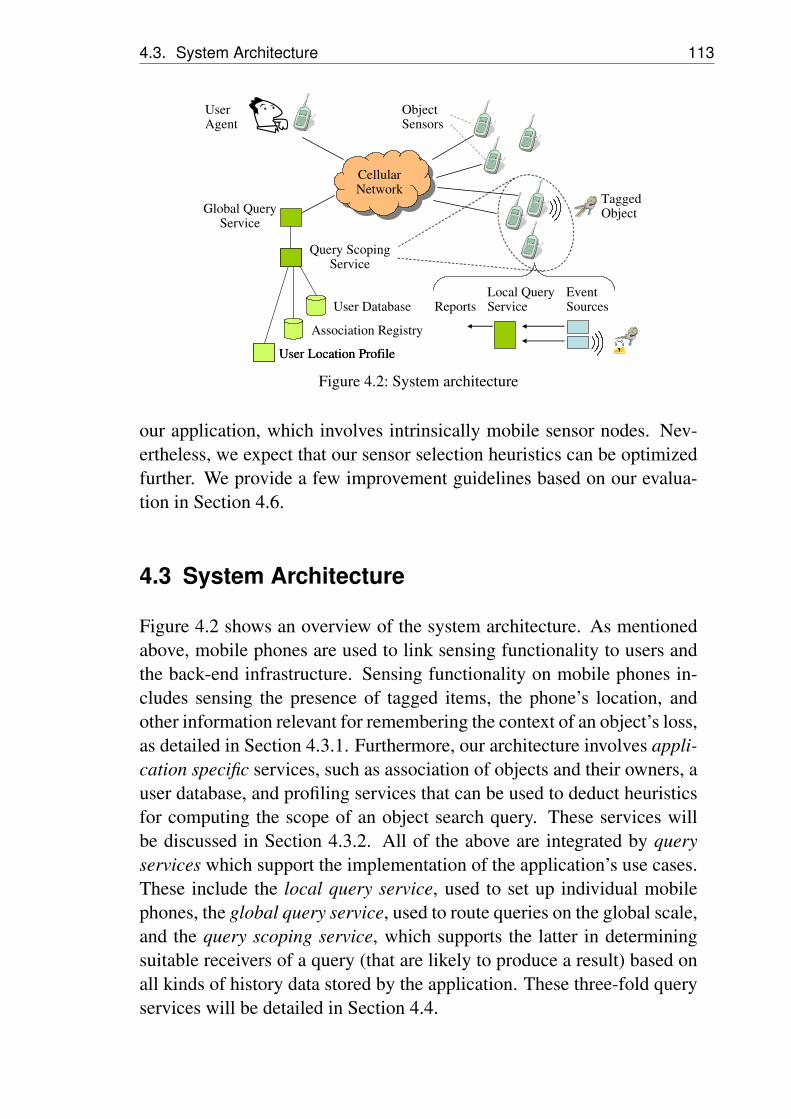
4.3. System Architecture 113
Global Query Service
Query Scoping Service
User Agent
User Database
Association Registry
Cellular Network
Cellular Network
User Location ProfileUser Location Profile
TaggedObject
Object Sensors
Event Sources
Local Query ServiceReports
Figure 4.2: System architecture
our application, which involves intrinsically mobile sensor nodes. Nev-ertheless, we expect that our sensor selection heuristics can be optimizedfurther. We provide a few improvement guidelines based on our evalua-tion in Section 4.6.
4.3 System Architecture
Figure 4.2 shows an overview of the system architecture. As mentionedabove, mobile phones are used to link sensing functionality to users andthe back-end infrastructure. Sensing functionality on mobile phones in-cludes sensing the presence of tagged items, the phone’s location, andother information relevant for remembering the context of an object’s loss,as detailed in Section 4.3.1. Furthermore, our architecture involves appli-cation specific services, such as association of objects and their owners, auser database, and profiling services that can be used to deduct heuristicsfor computing the scope of an object search query. These services willbe discussed in Section 4.3.2. All of the above are integrated by queryservices which support the implementation of the application’s use cases.These include the local query service, used to set up individual mobilephones, the global query service, used to route queries on the global scale,and the query scoping service, which supports the latter in determiningsuitable receivers of a query (that are likely to produce a result) based onall kinds of history data stored by the application. These three-fold queryservices will be detailed in Section 4.4.

114 Chapter 4. Query Scoping
4.3.1 Sensing Functionality
Apart from object sensors, which we assume to be integrated into eachmobile phone, we suppose that mobile devices have access to a variety ofadditional sensor information, for example, to a sensor determining thelocation of the user carrying the device.
Event Sources. All sensor information is encapsulated in application-specific software components which we name event sources. An eventsource generates events of a pre-determined type, either in a periodic man-ner or when a certain condition is met. Our system uses event sources thatgenerate an event whenever a tagged object comes in range or goes out ofrange of the device or when the device’s location changes. It also uses anevent source for persons who are within short wireless range of the userdevice.
In our prototype implementation, the location event source generates anevent every time the mobile phone’s cell identifier changes. Object tag-ging is implemented using BTnodes [BTn06], tiny devices equipped witha Bluetooth radio, and object sensing is realized using Bluetooth discov-ery. The in range and out of range event sources, respectively, generate anevent every time a new object is discovered by Bluetooth or a previouslyseen object has been missing in several rounds of discovery. Similarly,the person event source generates periodic events which contain a list ofnearby users based on the Bluetooth names of their phones.
Sensor Authentication. Both, object tags and devices representing per-sons, can restrict their visibility and allow only authenticated sensors todetect their presence. Such authentication is based on a shared secretwhich is exchanged between the actor initiating sensing and the sensedentity at an earlier time (the association service described below is usedfor this purpose). After the initial key exchange, protected entities canbe sensed only by sending an authenticated message. We discuss detailsof this concept which can be implemented on tags of a small form fac-tor [EHJ04] in Section 4.5.
Our implementation of sensor authentication is prototypical. Protectedpersons and objects are emulated by turning off visibility to Bluetoothdiscovery, while the Bluetooth MAC address takes on the role of a sharedsecret: Sensing polls (for persons or objects) consist of a connection at-tempt at the correct address.
4.3. System Architecture 115
4.3.2 Application Specific Services
In our architecture, three system services have been designed to take onspecific functionality mentioned in the object localization application.
Association. The association service serves three main purposes. First,it keeps track of associations between users and objects (Figure 4.1(a)shows the list of Alice’s associated objects). While objects can be de-tected by any object sensor in their initial state, after association, theyare detectable only within queries initiated by the object owner’s device.Second, user to object sensor association allows users to maintain a set ofobject sensors that are particularly relevant for them (e.g., object sensorswhich have been installed by the user at home or at work; Bob’s mobiledevice has previously been associated with Alice in the scenario depictedin Figure 4.1). Third, user to user association enables group access rightsto certain objects, but is also used as a basis for disclosing the identityof associated users to each other (in Figure 4.1(c), Alice is shown theidentity of Bob based on a previous association between them, otherwisethe notification would only contain the location of the object). Similarly,users may choose to be visible only to persons event sources set up byassociated users.
Location Profile. This optional service performs statistics on the loca-tions (such as the physical location or the observed network cells) inwhich users spend most of their time. This makes it possible to implementa search strategy (i.e., a query scoping strategy) which gives preference tosensors at these locations, assuming that they represent places that containpersonal belongings, such as a user’s work place or home.
Our prototype includes a rudimentary adaptation of a network-cell-based profiling system [LRT04] augmented with functionality for namingcertain network cells which are particularly relevant (such as ‘Office’ inFigure 4.1(c)).
User Database. We assume that the mobile network operator offers usersa database service in which application data such as previous reports ofcertain objects can be stored. The service can be used, for example, torecord a log of objects reported by an object sensor for later query. Sim-ilarly, it can be employed to store the details on the circumstances of anout-of-range event as required by the remember use case.
116 Chapter 4. Query Scoping
4.4 Query Services
The query services form the integrating central point of the system, wiringthe distributed components for the required application task. The back-end infrastructure hosts the global query service, which provides supportfor query dissemination, cost control, and validity management for userqueries. Moreover, each mobile device executes a local query servicedealing with handling data requests on the level of the local mobile phone.
The query scoping service supports the global query service by deter-mining which sensors should be involved in a wide area query, integratinginformation known at various application-specific services. For example,a query can be disseminated to a subset of associated users (based on in-formation stored in the association registry), to locations that are particu-larly relevant for the user (based on location profile data), or near locationswhere the object was observed in the past (based on the user’s database).
These query services are supported by a set of middleware serviceswhich are not detailed here. For instance, storage services are avail-able both on the mobile device and in the back-end infrastructure – andare also used to implement the user database and the association ser-vice. Their implementations including transparent data marshaling anddatabase interaction functionality for resource-constrained devices are de-scribed in [BL06]. Further, means for local event forwarding, wide areapoint to point messaging, and OSGi-based component execution plat-forms for both, the mobile device and the back-end infrastructure, havebeen implemented in our prototype. For details on these services, we re-fer to [FRB+07].
4.4.1 Query Service Interface
The query interface specifies the receivers of the query (its scope), thereceivers of produced reports (sinks), and, further, various limits on theinvolved query effort. The scope can either consist of a single mobiledevice (in the remember scenario the targeted device is simply the user’sphone) or a custom-implemented scope provider component (as in thefind use case). Scope providers, required to return a list of object sensorssorted by relevance, may be used to pass on a variety of search strate-gies to the global query service: For example, an association-based scopeprovider may simply return a list of previously associated object sensors,a location-profile-based scope provider would return sensors at locations
4.4. Query Services 117
where the user spends much time; the query scoping algorithm whichwe present in Section 4.4.2 also represents a scope provider componentthat can combine various search strategies. The reports generated by thequery, in turn, will be delivered to the specified sinks. Various systemservices may be wired as sinks: In the remember use case, reports will bedelivered to the local database on the user’s phone, in the find use case,reports cause a direct notification on the user interface.
Moreover, different effort limits can be issued with the query: cmax lim-its the monetary costs billed to the user, qmax the number of object sensorswhich are involved in the query, emax the total number of reports gener-ated by the query, and, finally, tmax the total time the query shall be active.The limits qmax and tmax are particularly relevant for the find example.Here, the global query service will distribute the query to the first qmaxsensors returned by the scope provider. The term qmax is equivalent to thenumber of messages sent by the global query service in the disseminationphase and can be used to limit the communication costs. The parametertmax may be used to specify the time that is usually required for an ad-equate search strategy to find an object and thus limits the search effortof inadequate strategies. Moreover, it allows for an iteration of differentsearch strategies of increasing costs, where the next strategy is initiatedafter an unsuccessful timeout of the previous. We will discuss suitablenumbers for tmax in Section 4.6.
To obtain suitable search strategies for wide-area queries of the findscenario is a challenge. Various heuristics can be used to distribute a queryto a relevant subset of object sensors. For example, one may distribute it tosensors near the location where the object was last observed. Similarly, allconceivable heuristics will be based on some kind of history data availablein the system.
To elaborate on this, we show a simple data model of our application inFigure 4.3: Objects are associated with users (object owners) by the as-sociation service and also with locations (e.g., cells) where an object hasbeen observed in the past. Users may choose to record a history of theirlocation on their mobile device (user history) or to enable the locationprofile service, which computes locations that a user visits frequently. Inthis simple model, locations are related to other locations via the neigh-borhood relation. Moreover, users can be associated with object sensorsthey often use (e.g., which they have installed in their office or car) andwith other users who are family, friends, or colleagues. Finally, the mobilenetwork operator keeps a database (object sensor registry) which stores

118 Chapter 4. Query Scoping
Location
Profile
OS
Registry
OS
Assoc.
User
Assoc.
Obj.
Assoc.
User
History
usrcell
Obj.
History
Neighb. loc usr
OS
obj
Figure 4.3: Example Data model
the current location (e.g., the current network cell) of object sensors (in-cluding certain mobile phones which can be used as object sensors as wellas stationary sensors).
In order to simplify its description, we omitted some details in the datamodel (most prominently a more refined location model). However, it issufficient to demonstrate that many conceivable search heuristics corre-spond to paths in Figure 4.3 from an entity of type object at the top toentities of type object sensor, which should be queried for the object. Forexample, we can query object sensors which:
I) Are near the location where the object was last seen.II) Are near locations recently visited by the user.
III) Are near locations where the user spends a large amount of her/histime.
IV) Are associated with the object owner (as in Figure 4.1).V) Match the above strategies III and IV for a different (associated) user,
such as a family member, or even for a friend of a friend, etc.
While, intuitively, none of these heuristics can guarantee success, theyall incorporate sensible assumptions on where users keep personal be-longings and where these are generally left. Note how each heuristics rep-resents a path in the data model of Figure 4.3: Heuristics I corresponds tothe path (obj-loc-object sensor) on the left, while heuristics V correspondsto the path obj-usr-usr-loc-object sensor.
Based on these considerations, a data model is a suitable means to ex-press the real-world links between various types of data stored by the sys-tem, and can be used to generate a variety of search strategies – includingall of the above. In particular, the application programmer may assign
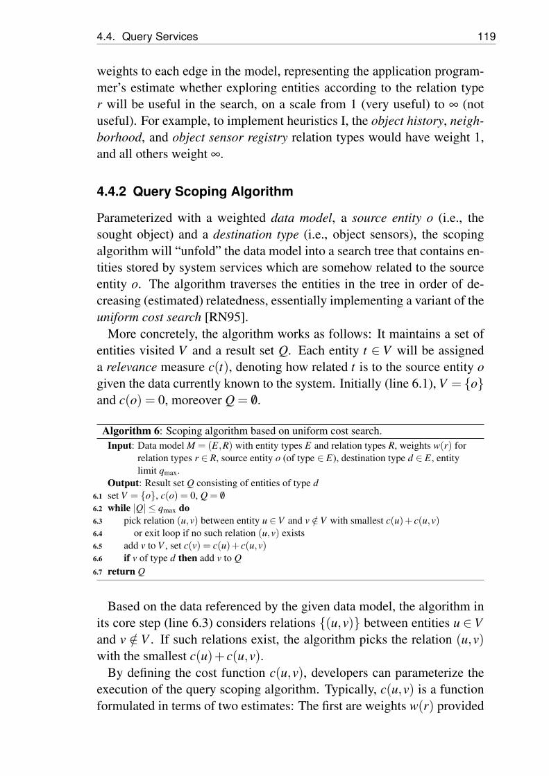
4.4. Query Services 119
weights to each edge in the model, representing the application program-mer’s estimate whether exploring entities according to the relation typer will be useful in the search, on a scale from 1 (very useful) to ∞ (notuseful). For example, to implement heuristics I, the object history, neigh-borhood, and object sensor registry relation types would have weight 1,and all others weight ∞.
4.4.2 Query Scoping Algorithm
Parameterized with a weighted data model, a source entity o (i.e., thesought object) and a destination type (i.e., object sensors), the scopingalgorithm will “unfold” the data model into a search tree that contains en-tities stored by system services which are somehow related to the sourceentity o. The algorithm traverses the entities in the tree in order of de-creasing (estimated) relatedness, essentially implementing a variant of theuniform cost search [RN95].
More concretely, the algorithm works as follows: It maintains a set ofentities visited V and a result set Q. Each entity t ∈ V will be assigneda relevance measure c(t), denoting how related t is to the source entity ogiven the data currently known to the system. Initially (line 6.1), V = {o}and c(o) = 0, moreover Q = /0.
Algorithm 6: Scoping algorithm based on uniform cost search.Input: Data model M = (E,R) with entity types E and relation types R, weights w(r) for
relation types r ∈ R, source entity o (of type ∈ E), destination type d ∈ E, entitylimit qmax.
Output: Result set Q consisting of entities of type dset V = {o}, c(o) = 0, Q = /06.1
while |Q| ≤ qmax do6.2
pick relation (u,v) between entity u ∈V and v /∈V with smallest c(u)+ c(u,v)6.3
or exit loop if no such relation (u,v) exists6.4
add v to V , set c(v) = c(u)+ c(u,v)6.5
if v of type d then add v to Q6.6
return Q6.7
Based on the data referenced by the given data model, the algorithm inits core step (line 6.3) considers relations {(u,v)} between entities u ∈Vand v /∈ V . If such relations exist, the algorithm picks the relation (u,v)with the smallest c(u)+ c(u,v).
By defining the cost function c(u,v), developers can parameterize theexecution of the query scoping algorithm. Typically, c(u,v) is a functionformulated in terms of two estimates: The first are weights w(r) provided
120 Chapter 4. Query Scoping
by developers to assess whether the relation type r which stores the re-lation (u,v) is assumed useful in the search. Moreover, implementatonsof c(u,v) commonly take into account a second estimate, referred to asg(u,v), by which the service that stores (u,v) may provide a relative orderamong different entities v related to u. In particular, g(u,v) estimates therelevance of v given that u is relevant for the search. For example, thelocation profile service could estimate g(user, loc) for different locationsusing statistics on the amount of time the user spends in them. For the ob-ject history relation, it is intuitive that the latest location where the objectwas observed is the most relevant. We will provide concrete examples forc(u,v) in Section 4.4.3.
In the remainder of the loop, the algorithm adds v to the set of visitedentities V , updates the relevance estimate c(v) of v (line 6.4), and adds vto the result set if it is of type destination type (line 6.5). The algorithmrepeats these steps until up to entity limit related entities have been found,and then returns Q (if the chosen destination type is object sensor, theentity limit corresponds to the limit on queried sensors qmax).
A requirement for the edge cost function c(u,v) is that it shall returnvalues on the same scale ranging from 1 (for very related) to ∞ (for un-related). If this is the case, the shortest path sums c(t) maintain the samesemantics. Based on the costs c(u,v), the algorithm explores the mostrelevant relations first, and the result list Q contains entities t of type des-tination type in order of increasing c(t), that is, in order of decreasingrelatedness to the start entity o.
While based on classic search methods, the presented approach lends it-self well to distributed data sources: Each system service that implementsa relation type accessed by the algorithm is required to provide a singleinterface method next(u), which allows to iterate through the entities v re-lated to u in the order of increasing c(u,v). Note that both the runtimeand the space complexity of the algorithm depend on the data referencedin the given data model.
The algorithm implements a variant of uniform cost search [RN95]based on the edge costs c(u,v). The result set Q contains entities t oftype destination type in order of increasing cost c(t), that is, in order ofdecreasing relatedness to the start entity o. Compared to uniform costsearch, our approach does not expand all children of a node u at a time asthere are potentially too many, due to several relations relevant for u anda potentially huge list of related entities provided by each one. Instead, ateach step, we only add a single child entity v to the search tree.
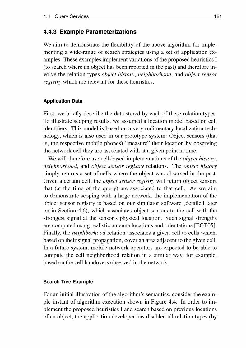
4.4. Query Services 121
4.4.3 Example Parameterizations
We aim to demonstrate the flexibility of the above algorithm for imple-menting a wide-range of search strategies using a set of application ex-amples. These examples implement variations of the proposed heuristics I(to search where an object has been reported in the past) and therefore in-volve the relation types object history, neighborhood, and object sensorregistry which are relevant for these heuristics.
Application Data
First, we briefly describe the data stored by each of these relation types.To illustrate scoping results, we assumed a location model based on cellidentifiers. This model is based on a very rudimentary localization tech-nology, which is also used in our prototype system: Object sensors (thatis, the respective mobile phones) “measure” their location by observingthe network cell they are associated with at a given point in time.
We will therefore use cell-based implementations of the object history,neighborhood, and object sensor registry relations. The object historysimply returns a set of cells where the object was observed in the past.Given a certain cell, the object sensor registry will return object sensorsthat (at the time of the query) are associated to that cell. As we aimto demonstrate scoping with a large network, the implementation of theobject sensor registry is based on our simulator software (detailed lateron in Section 4.6), which associates object sensors to the cell with thestrongest signal at the sensor’s physical location. Such signal strengthsare computed using realistic antenna locations and orientations [EGT05].Finally, the neighborhood relation associates a given cell to cells which,based on their signal propagation, cover an area adjacent to the given cell.In a future system, mobile network operators are expected to be able tocompute the cell neighborhood relation in a similar way, for example,based on the cell handovers observed in the network.
Search Tree Example
For an initial illustration of the algorithm’s semantics, consider the exam-ple instant of algorithm execution shown in Figure 4.4. In order to im-plement the proposed heuristics I and search based on previous locationsof an object, the application developer has disabled all relation types (by

122 Chapter 4. Query Scoping
setting c(u,v) = ∞) except for the relevant relation types object history,neighborhood, and object sensor registry.
Each enabled relation type can be used to generate child entities usingthe next(u) method, which the algorithm invokes at the service imple-menting the respective relation type. Starting with the sought object o,only the object history relation type is enabled, for which a call to next(o)returns the location where the object has been seen last, in this example incell1. Given a cell entity, object sensor registry may generate child enti-ties representing object sensors in that cell, while neighborhood generateschild nodes which are other, neighboring, cells. The other relations willnever contribute any child entities because they have infinite edge costs.
Cell2Cell1
Sought object
…
Object
History
Object Sensor
Registry
Neighbourhood
Cell4 …
…
…
0
0 500
1
200 200
2 1 2
1 …Object Sensors
201…
1
201 …
( , )c u v �
2
200
2
…
500
201
R∈
V∈
V∉
Notation
( )c t �Cell3
200
Figure 4.4: Example search tree generated by three relation types
As the algorithm’s basic step will always add the edge leading to thesmallest c(t), one may express preference for one relation type over an-other by means of the edge cost function c(u,v). In the shown execution,because c(cell1,∗) is set to 200 for the neighborhood relation, the algo-rithm explores (and adds to the scope) 200 object sensors in cell1 first, andlater explores object sensors in cell1’s neighboring cells cell3 and cell4.
Edge Cost Functions
In the following, we will give parameterizations for the edge-cost func-tions c(u,v) which are able to implement a range of different search strate-gies. Although arbitrarily complex implementations of the cost functionc(u,v) could be provided by the system designer, in the examples below,we will use a simplified form of c(u,v) which already suffices to formu-late a range of examples. In our examples, c(u,v) has the form
c(u,v) = a(r)+b(r)×g(u,v) (4.1)

4.4. Query Services 123
in which a(r) and b(r) are parameters defining the relevance of the rela-tion type r. Moreover, in this example implementation of c(u,v), g(u,v)corresponds to the index of v in the list of entities related to u – sortedby decreasing relevance. For example, the object history relation wouldset g(obj,cell1) = 1 if cell1 were the location where obj was last seen,g(obj,cell2) = 2 for a second, less relevant, location cell2 where the ob-ject was seen earlier. Note that g(u,v) could implement much more fine-grained estimates of the importance of different entities v that are relatedto an entity u. Nevertheless, this simple implementation of g(u,v) (return-ing v’s place in the list of related entities) already allows for a range ofheterogeneous search strategies, as we will show below.
As the algorithm implements uniform cost search based on c(u,v), thecost parameters a(r) and b(r) have the following semantics:
a(r) Defines how the first entity v contributed by r will be prioritizedcompared to other parts of the search tree. Once the algorithm hasexplored u, it will grow other parts of the search tree by a(r) beforeit adds v. The higher a(r) in c(u,v), the less important is r comparedto other relations contributing children to u and to other parts of thetree.
b(r) Defines how an additional entity w contributed by r will be priori-tized compared to other parts of the search tree. Such an entity w willbe added to the tree only after all other parts of the tree have grownby b(r). The higher b(r), the less important are additional entitiescontributed by r.
Searching based on the Object’s History
The two weight parameters a(r) and b(r) can be illustrated using the ex-ample of Figure 4.5(a), which implements a variation of search strategy I:On the one hand, as the strategy involves searching at locations wherethe object was observed in the past, the object history relation is relevantin the search. Therefore, the algorithm should add the first related entityimmediately, and a(object history) = 0. On the other hand, consideringadditional locations further back in time is considered less useful in thisexample, therefore, b(ob ject history) is high in order to let c(u,v) forsuch entities grow fast.
More specifically, based on the algorithm’s uniform cost property, theratio between b(object history) = 500 and b(object sensor registry) = 1
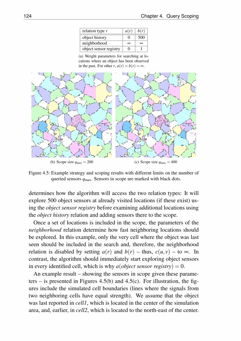
124 Chapter 4. Query Scoping
relation type r a(r) b(r)object history 0 500neighborhood ∞ ∞
object sensor registry 0 1
(a) Weight parameters for searching at lo-cations where an object has been observedin the past. For other r, a(r) = b(r) = ∞.
(b) Scope size qmax = 200 (c) Scope size qmax = 400
Figure 4.5: Example strategy and scoping results with different limits on the number ofqueried sensors qmax. Sensors in scope are marked with black dots.
determines how the algorithm will access the two relation types: It willexplore 500 object sensors at already visited locations (if these exist) us-ing the object sensor registry before examining additional locations usingthe object history relation and adding sensors there to the scope.
Once a set of locations is included in the scope, the parameters of theneighborhood relation determine how fast neighboring locations shouldbe explored. In this example, only the very cell where the object was lastseen should be included in the search and, therefore, the neighborhoodrelation is disabled by setting a(r) and b(r) – thus, c(u,v) – to ∞. Incontrast, the algorithm should immediately start exploring object sensorsin every identified cell, which is why a(object sensor registry) = 0.
An example result – showing the sensors in scope given these parame-ters – is presented in Figures 4.5(b) and 4.5(c). For illustration, the fig-ures include the simulated cell boundaries (lines where the signals fromtwo neighboring cells have equal strength). We assume that the objectwas last reported in cell1, which is located in the center of the simulationarea, and, earlier, in cell2, which is located to the north-east of the center.
4.4. Query Services 125
Because b(object sensor registry) is low compared to b(object history),additional sensors in cell1 are added to the scope before cell2 is consid-ered (Figure 4.5(b)). If one increases qmax (the limit on the number ofsensors) to have the algorithm return a larger scope, it will first add 500sensors in cell1 to the scope, and then additional sensors from cell2 (Fig-ure 4.5(c)).
Searching Neighborhoods
The above example can be altered in various ways. To have the algo-rithm also include neighboring cells in the search, e.g., to allow for thecase that the locations returned by object history are imprecise, the pa-rameterization of the neighborhood relation can be changed as shown inFigure 4.6(a). Setting a(neighborhood) = 200 causes the algorithm tobegin adding sensors from neighboring cells to the scope once about 200sensors associated with already known cells have been added by means ofthe object sensor registry relation.
relation type r a(r) b(r)object history 0 500neighborhood 200 0object sensor registry 0 1
(a) Weight parameters for searching wherethe object has been observed in the past andat neighboring locations as well. For otherr, a(r) = b(r) = ∞.
(b) Scope size qmax = 220 (c) Scope size qmax = 2000
Figure 4.6: A search strategy based on the location of the last report and its neighborhood

126 Chapter 4. Query Scoping
Note that Figure 4.4 (introduced above) corresponds to such a param-eterization (Figure 4.6(a)) and (roughly) to the results shown in Fig-ure 4.6(b). It shows the instant of execution after the algorithm has addedall object sensors with c(t) ≤ 200 to the result set Q, and is about to addobject sensors from neighboring cells in a uniform manner (in Figure 4.4the next basic step will add a sensor in cell4). Figure 4.6(c) demonstratesthe effect of an expanding scope size qmax. The figure shows how, basedon the uniform cost search semantics, cells within two hops are explored.This is based on the implications of the fraction b(object history)
a(neighborhood) > 2: Thealgorithm can begin expanding neighbors twice before an additional loca-tion from the object history relation would be added to the scope.
Because b(neighborhood) = 0, the order g(cell1,v) in which neighborsof cell1 are returned by the neighborhood relation does not have an impacton the execution of the algorithm: All neighboring cells are consideredequally important and therefore child nodes (sensors in these cells) areadded to the result set in equal proportions.
Ordering Neighbors
If an order of neighboring cells should be relevant, e.g., if based oninformation stored in the system some cells can be assumed “closer”to cell1 than others, the developer may assign more significance tothe order g(u,v) returned by the neighborhood relation using a higherb(neighborhood) parameter as shown in Figure 4.7(a).
Based on the uniform cost search property, 50 object sensors from ob-ject sensor registry will be added to the result set before the next cellis retrieved from the neighborhood relation. This is reflected in the re-spective scoping results shown Figure 4.7(b) where the scope is focusedaround the original cell and two (assumedly most relevant) neighbors. Ex-panding the scope to more sensors adds more neighboring cells, and, oncethe scope is large enough, the algorithm starts adding sensors at the sec-ond location returned by the object history relation (Figure 4.7(c)). Notethat cell neighborhood is defined as cells sharing a common border and,due to non contiguous cell coverage, some cells are considered neigh-bors although this is not apparent in the figures. Further, note that theorder g(u,v) among neighboring cells is chosen randomly in this examplewhile, in a future system, neighboring cells could be prioritized by variousprofiling services, e.g., based on data from the location profile [LRT04]: Ifusers tend to switch between neighboring cells frequently, these cells are

4.4. Query Services 127
relation type r a(r) b(r)object history 0 500neighborhood 200 50object sensor registry 0 1
(a) Variation of the parameters to take into ac-count the order in which cells are returned bythe neighborhood relation; for all other relationtypes r, a(r) = b(r) = ∞
(b) qmax=400 (c) qmax=1000
Figure 4.7: Search strategy taking the order of neighboring locations into account
likely to cover the same physical location and, therefore, are both likelyto be useful in the search.
A Combined Search Strategy
We close with a last example, which demonstrates how the algorithm mayimplement combined search strategies that are based on multiple paths inthe data model. In the previous parameterizations (e.g., in Figure 4.6(a)),the neighborhood relation was prioritized compared to the object historyrelation type). To state that the search should explore previous locationsof the object as well, one could decrease b(object history), and thereforeimplement a mixed strategy based on data on an object’s previous loca-tions and on the neighborhood of these locations.
Such a combined strategy is shown in Figure 4.8(a). Settingb(object history) = 100 demands that the search should consider an ad-ditional location where the object was reported, once 100 sensors havebeen added at previous locations. Moreover, the ratio a(neighborhood)
b(object history) im-plies that a second history location is considered in the scope, before the
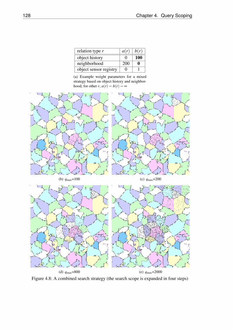
128 Chapter 4. Query Scoping
relation type r a(r) b(r)object history 0 100neighborhood 200 0object sensor registry 0 1
(a) Example weight parameters for a mixedstrategy based on object history and neighbor-hood; for other r, a(r) = b(r) = ∞
(b) qmax=100 (c) qmax=200
(d) qmax=800 (e) qmax=2000
Figure 4.8: A combined search strategy (the search scope is expanded in four steps)
4.4. Query Services 129
neighborhood relation will start contributing neighboring cells and addsensors near these locations to the resulting scope Q.
We show a set of scopes computed according to Figure 4.8(a) in Fig-ures 4.8(b)-4.8(e). The results highlight how the algorithm adaptivelyintegrates different search strategies while the user expands the size ofthe query scope qmax. When the scope size is low (in Figure 4.8(b)) thestrategy with highest preference (to include sensors at the location wherethe object was reported last) is considered. If the system cannot find theobject in this small scope, the user might choose to increase qmax. Thiswill produce an enlarged scope (Figure 4.8(c)) that includes sensors at asecond location while still prioritizing the first. Once even more sensorsare permitted, and because no additional sensors are available apart fromthe most probable locations (cell1 and cell2), the scope expands by meansof the neighborhood relation only (Figures 4.8(d) and 4.8(e)).
4.4.4 Discussion
In comparison with previous chapters, application requirements havedriven the design of a very specific role assignment algorithm which as-signs the role sensing to nodes inside the computed scope.
One the one hand, requirements included allowing users to formulate(and even automatically generate) a wide range of strategies for selectingsensing nodes. To achieve this, the algorithm was required to be able totake into account arbitrary information available at system services. Thishas led to an interface, described above, which is based on data modelsof the application domain – annotated with weight parameters that definethe relevance of relations in the model.
On the other hand, efficient communication between different sourcesof data used by the query scoping algorithm is required, because the re-lations driving the algorithm’s execution are stored at distributed appli-cation services. Therefore, the interface between the algorithm and datasources has been streamlined to a simple next(u) method, which is calledonly once for every related entity.
These requirements have been met well. Some open issues, however,remain.
Semantics
The first issue is related to the semantics of a given set of parameterizedfunctions {c(u,v)}. While these functions provide a flexible configura-

130 Chapter 4. Query Scoping
tion interface, the effects of a given function definition c(u,v) are not apriori well understood by developers. Instead, the exported semanticsare closely bound to the algorithm’s execution. In contrast, the Booleanpredicates used in the generic role assignment specifications described inChapter 2 are a much more intuitive concept. Similarly, the implicationsof the parameters issued to the facility location algorithms of Chapter 3can be considered well-understood concepts: They represent an estimateof the cost of either operating a hub or communicating with a hub in agiven epoch of network operation.
In comparison, the understanding of the provided levers to the abovequery scoping algorithm may be less intuitive. This seems to be a featureas well as a drawback. Using the functions c(u,v), the developers areprovided a very fine-grained control over the algorithm’s execution. Inturn, for specialized search strategies, the developers must perform animportant translation between the search strategy they have in mind andthe respective design of the functions c(u,v).
Note, however, that this is mostly the case if multiple paths through thedata model are explored in combined search strategies. If a single pathis followed instead, as is mostly the case in the heuristics I-V describedin Section 4.4.1 above, the parameterization is much simpler, mostly justenabling or disabling certain relationship types.
Moreover, we argue that even for more involved strategies, an appli-cation developer is provided a valuable configuration tool that combinesdistributed data sources quickly and effectively. When combining differ-ent paths through the data model, care must be taken to make the relevanceestimates g(u,v) (issued by different relations) comparable – by means ofweights attached to the respective cost functions.
Finally, while the above algorithm is flexible and requires only a limitedamount of communication between distributed data sources, compared toother search algorithms, the described approach involves an additional ap-proximation heuristic: During search, it considers only the shortest pathto a given entity, and disregards all longer paths that may be discoveredlater on during algorithm execution. This is a viable approach and alsocrucial for enabling efficient exploration of the distributed data sources.However, it neglects the fact that a large number of ignored long pathscould imply that an entity t is more relevant than it is apparent in thelength of the shortest path c(t).
More sophisticated algorithms (such as PageRank [BP98]) let the nodeweight c(t) represent a weighted sum of all paths to t, which is computed
4.4. Query Services 131
by solving a system of linear equations. Such algorithms require thatall paths are explored before computing the rank (in terms of relevance)of an individual sensor. In contrast, our application requires that sensi-tive data stores (e.g., association or the location profile) can be stored onuser’s devices to protect the user’s privacy (cf. Section 4.5). Therefore,the exploration of all relevant paths at the same time would not be pos-sible – unless one gathers all data in a centralized database. We perceivesuch centralized data collection as a significant disadvantage based on itsprivacy implications, in particular, given the large amount of personal in-formation our system may collect on its users’ everyday lives.
Space Complexity
A second issue of the presented algorithm is that it inherits the exponen-tial space complexity present in any breadth-first search. This does notrepresent a significant disadvantage in our application domain, however:Firstly, the costs of an object search billed to the user will most likelybe proportional to the number of queried object sensors (due to commu-nication costs). As only a constant (user-defined) budget is granted, atmost a constant number of object sensor entities will be in the searchtree (as any visited object sensor will be queried during search). Sec-ondly, the number of intermediate entities (like locations) in the tree canalso be limited by raising the weight parameters of individual relations,which will re-configure the algorithm to explore “deeper” paths earlierand reach object sensor entities faster. In the example execution shownin Figure 4.8(a), setting a(neighborhood) higher would force the algo-rithm to explore many object sensors at already known locations beforeincluding additional locations in the search.
4.4.5 Global Query Service
In the following, we will discuss how the presented algorithm is employedby the global query service to implement the search strategies I-V in prac-tice. For this, note that search strategies I-III employ the object sensorregistry relation, which associates a set of locations L to a set of objectsensors near them. Due to user mobility, however, the object sensors nearthe set L will change with time. Therefore query scoping is decoupledfrom the actual movements of users and their object sensors. That is,when heuristics I-III are implemented, location will be the destinationtype parameter passed to the search algorithm. The returned set of loca-
132 Chapter 4. Query Scoping
tions L, for example a set of cells, is then passed on to the global queryservice, which will distribute the query at these locations. The globalquery service is then concerned with maintaining a computed query scopeover time while observing the cost control parameters (qmax, tmax, emax,and cmax) specified at the query interface.
If search strategy IV is chosen, a set of object sensors is determined bythe scoping algorithm. Here, a query will be distributed to the first qmaxsensors returned by the scoping algorithm and be active for at most tmaxtime.
If search strategies I-III are chosen, the scoping algorithm will not di-rectly return a set of object sensors, but a set of locations, as mentionedabove. In the basic location model we employ, these can either be a setof cells (the most basic localization already available on the phone) or aset of geographic points (if phone localization is more precise) togetherwith an associated measurement error. Because the set of object sensorsassociated with these locations may change over time, our system installs(or un-installs) a query at sensors which come close to (or, respectively,depart from) these locations. Whether a sensor s is close to the returnedlocations is defined by the implementation of a predicate f (which mapss to either true or false).
Depending on the way locations are modeled, we use two different im-plementations of f (s). Given a set of cells C, f (s) will be true if the mo-bile phone (with its object sensor s) is currently served by any of the cellsin C. Note that this information is already available at the mobile networkoperator, that is, it can be accessed on the server side of our infrastructurewithout incurring additional communication costs.
In case the mobile devices are equipped with more accurate position-ing means, the locations returned by query scoping will instead be a setof geographic points P. Here, f (s) will be true if the current positionmeasured by a mobile phone’s object sensor s is within a certain range raway from the points P. This range r will depend on the error incurred atthe positioning sensor when the points in P were measured (we will dis-cuss a concrete implementation in Section 4.6). Note that such additionalpositioning information will only improve the efficiency of query dissem-ination if positioning information of all object sensors is already known ata database on the server. Otherwise, it would be inefficient to propagateall object sensor positions to the server before query dissemination, andtherefore a different approach is chosen: The query is distributed to objectsensors in a set of cells C which “cover” the whole area surrounding the

4.5. Privacy Considerations 133
points P (the actual object sensor will be turned on only later, once thepredicate f (s) evaluates to true). Note that the total number of distributedqueries is now the same as if locations were a set of cells C.
When installing queries for such location-based strategies I-III, the totalnumber of object sensors at which a query will be installed (qtotal) is madeup of two parts, qtotal = qinit + qmob. Here, qinit denotes the number ofusers queried initially at the time the query is issued – chosen out of theinitial query scope Sinit = {s| f (s) = true}. In addition to qinit, the querywill be installed at a second set of sensors qmob for which f (s) becomestrue while the query is active.
After a query installation at an object sensor s, object sensing will beperformed continuously until tmax expires. The mobile device associatedwith s un-installs the query autonomously either when f (s) becomes falseor when tmax expires.
A query is declared successful, if some object sensor s reports havingfound o at time treply with treply ≤ tmax. The current position of s representsthe location at which the object was found and will be included in thereply issued to the user. A query is terminated without success, once thequery timeout tmax is reached.
4.5 Privacy Considerations
The query service, presented in the previous sections, makes use of a widevariety of personal user data. In the following, we describe a few privacyenhancing features of our system.
Most prominently, tagged objects and persons can be protected frombeing sensed by unauthorized users as proposed in [EHJ04]. This protec-tion is based on a shared secret x, which is known both at an authorizeduser device U and at the sensed entity (e.g., at a tagged object o). Withquery initiation, U may issue a zero-knowledge authentication message(ZAM), say m, in which the shared secret x is made oblivious by meansof a random session key r and a current time stamp d. The ZAM is for-matted such that the receiving tagged object o can recover r as it knowsx and also receives an authentication proof that U truly knows x1. Basedon this feature, if authentication fails, o simply does not reply. Moreover,o will only reply to the first reception of m. Therefore, an adversary Acannot easily make use of forwarded queries to locate objects which havebeen lost by other users in public spaces. To be effective, A must not onlyhave been forwarded the find query containing m but also be the first to
134 Chapter 4. Query Scoping
sense o using m. To achieve this, A needs to control an infrastructure ofobject sensors that finds objects faster than the infrastructure provided byregular system users – in most cases an unrealistic assumption.
As noted, a ZAM represents a permit for sensing once. For use cases inwhich sensing of an object or person o must be performed multiple timeswithin a given query (e.g., delegate or gate), there are three options: Thefirst is to let an authorized user device U re-issue a proper ZAM everytime, which requires repeated end-to-end communication between o andU . The second is to entrust the shared secret to the global query service(run by the mobile network operator on the back-end server) which maythen issue authentication messages on its own. The third is to propagatethe shared secret even further to the remote sensor R (such as the objectsensor employed in the gate scenario) for the time of query execution.The latter two options lower the communication overhead (the overheadof the third option is lowest) but require that the user is confident that theentrusted entity (e.g., the remote sensor R) does not leak the shared secretduring the time of the query. After query termination, the shared secret xmay be changed – such a change could be propagated to multiple users Upreviously associated with o using the same authentication protocol.
A second privacy enhancing feature of our system is the component de-ployment infrastructure, which allows to re-configure the execution plat-form of services containing sensitive information within the application.That is, the association registry or the location profile, which should en-hance object search functionality, could be executed on the user’s mobiledevice instead of the server back-end, giving users full physical controlover their data. Similarly, deployment of the location profile service couldbe completely omitted – based on user preferences.
Some potential privacy threats, however, remain. One threat is sharedby any system providing wide-area object localization, namely, that anadversary may attach a properly associated object to some person he orshe wishes to track. Avoiding such threats is hard as they are related to thecore functionality of the envisioned system. Possible approaches wouldbe to limit the frequency of user queries, or make repeated consecutivequeries for an object expensive. Vice versa, adversaries may leave an ob-ject at a known location, and then check whether associated users arriveat this location. Here, the required transparency can be obtained by mak-
1A ZAM has three parts: m = (d;r xor hash(d xor x); hash(r xor x)). Using d and part two, o cancompute r. Using r, o can check part three, which confirms that the sender truly knew the secret x. Fordetails we refer to the original paper [EHJ04].
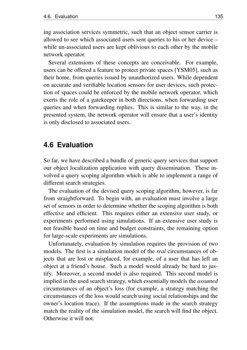
4.6. Evaluation 135
ing association services symmetric, such that an object sensor carrier isallowed to see which associated users sent queries to his or her device –while un-associated users are kept oblivious to each other by the mobilenetwork operator.
Several extensions of these concepts are conceivable. For example,users can be offered a feature to protect private spaces [YSM05], such astheir home, from queries issued by unauthorized users. While dependenton accurate and verifiable location sensors for user devices, such protec-tion of spaces could be enforced by the mobile network operator, whichexerts the role of a gatekeeper in both directions, when forwarding userqueries and when forwarding replies. This is similar to the way, in thepresented system, the network operator will ensure that a user’s identityis only disclosed to associated users.
4.6 Evaluation
So far, we have described a bundle of generic query services that supportour object localization application with query dissemination. These in-volved a query scoping algorithm which is able to implement a range ofdifferent search strategies.
The evaluation of the devised query scoping algorithm, however, is farfrom straightforward. To begin with, an evaluation must involve a largeset of sensors in order to determine whether the scoping algorithm is botheffective and efficient. This requires either an extensive user study, orexperiments performed using simulations. If an extensive user study isnot feasible based on time and budget constraints, the remaining optionfor large-scale experiments are simulations.
Unfortunately, evaluation by simulation requires the provision of twomodels. The first is a simulation model of the real circumstances of ob-jects that are lost or misplaced, for example, of a user that has left anobject at a friend’s house. Such a model would already be hard to jus-tify. Moreover, a second model is also required. This second model isimplied in the used search strategy, which essentially models the assumedcircumstances of an object’s loss (for example, a strategy matching thecircumstances of the loss would search using social relationships and theowner’s location trace). If the assumptions made in the search strategymatch the reality of the simulation model, the search will find the object.Otherwise it will not.

136 Chapter 4. Query Scoping
10
C
B
D
1225 1244 544 444 558 629
623 529 372 363
1 2 3
9
8 7
4 5 6
Figure 4.9: Experiment setup: Average reply times (in seconds) for the 10 tagged objectsin different rooms
Based on these considerations, in the remainder of this chapter, weavoid generating full models of the system’s future use. Instead, in theevaluations of this section, we assume that the employed search strategiesare in fact correct. Such evaluation allows to assess the performance of auser-carried infrastructure for finding an object, given that the user will atsome point come up with a correct search strategy.
In the following, we therefore provide an evaluation of the performanceof our system using two strategies mentioned in the course of the chapter– using a small real-world experiment and a set of simulations.
4.6.1 Real-world Experiment
We first come back to the scenario from the introduction of this chapter(Figure 4.1), where the user is at home and tries to verify the whereaboutsof a given object which was left at the office. The mobile phones of theuser’s officemates (e.g., Bob) are registered with the association serviceand thus are considered relevant object sensors.
Our experiment was performed with four users working on the samefloor. The users were given mobile phones running the object search pro-totype already tasked to perform continuous object sensing for all objects(using repeated Bluetooth discovery) and to report their findings in reg-ular intervals to the back-end database. Similarly, 10 BTnodes [BTn06]representing tagged objects were distributed in various rooms of the samefloor. Figure 4.9 shows the experiment’s setup (tagged objects are shownas numbered circles while the offices of the four participating users areshaded).
Note that while Bluetooth may be too expensive and battery-intensive tobe used as an object tagging technology in a practical system, it neverthe-

4.6. Evaluation 137
less allows to test whether, given a better-suited technology with similarradio range, the mobility of a few office colleagues suffices to detect agiven object in reasonable time.
During four consecutive days, all sensor readings entered the databaseas (user, time, obj_id) tuples. We considered only core office hours, that is,readings reported after the fourth user arrived in the morning and beforethe first left at night. This resulted in 30 hours of data. Based on thesedata, the reply time of a search query for a given object o issued at anarbitrary time tq to the four office colleagues can be computed as tr =tDB− tq, where tDB is the time of the next database entry on the object o.
Based on this consideration, we computed the average reply time foreach object, assuming that queries for this object were distributed uni-formly over the experiment time. In order to save messaging costs, userdevices cached seen objects and only re-reported them to the database 10minutes after their last report on the same object. This way, even if anobject sensor has seen the object continuously, the resulting reports willyield an average query reply time of 5 minutes instead of zero.
For each object, Figure 4.9 shows the average reply time in seconds.Intuitively, we expect to obtain low values for objects with a participatinguser in the same room (objects 3, 5, 8, and 9). Further, note that thebest results were obtained for objects close to the printer and the coffeemachine (objects 7 and 8), while objects in rooms that were not visited bythe participants during the experiment yield worse results.
We show a cumulative density curve of the observed reply times forobject 2 (with worst results), object 7 (with best results), and the averageover all objects in Figure 4.12(a) further down. In all cases, reasonablesuccess rates (about 80%) could be obtained with a maximum query timetmax of 30 minutes.
4.6.2 Simulation Model
In our experiments described above, we focused on a small and confinedsearch area and query scope. In the remaining evaluations, we use simula-tions to investigate the characteristics of an object search system operatingin the wide-area with a larger user base – to provide design guidelines fora future realistic system.
As we mentioned, adequate models of a large-scale execution environ-ment are difficult to obtain, as these must consider many aspects of dailylife. To provide an accurate basis for system design, models must include

138 Chapter 4. Query Scoping
the number of participating users, the frequency at which these users loseor search for certain objects, particular scenarios where objects are lost,and the number of tagged objects owned by each user. Intuitively, such amodel contains many parameters which cannot be influenced by the sys-tem designer. We refer to such parameters as environmental parameters.Our approach to these parameters is to investigate a significant portion ofthis rather vast parameter space.
In contrast, there are some design parameters which determine the sys-tem’s performance and can more or less directly be set and varied by thesystem developer. These include the size of the search scope (the numberof users who participate in searching for an object), the sensing range ofan object sensor (which can be influenced by employing more expensivetag and object sensing hardware), or the timeout used for queries. Forthese design parameters we aim to find the most appropriate values, i.e.,the parameter settings which can implement object search with the leastcommunication overhead for a given success rate.
Scenario. In the evaluated scenario, a user misplaces an object o and laterissues a search query to the global query service. We assume that at thetime the object left the range of the object sensor, the user’s mobile devicerecorded its location p. This location p is used as a hint in the search(implementing heuristics I presented in Section 4.4.2). We evaluate twoversions, a cell-based version in which p is a cell, and a position-basedversion in which p is a geographic point measured with a certain error. Inboth versions, query scoping is performed as described in Section 4.4.5.
Metrics. The main metric we observe is the success rate of our system.This rate corresponds to the fraction of queries for which a notificationfrom some object sensor is received within the query timeout tmax. Fur-ther, we examine the overhead for query distribution qtotal including thepart qmob which is caused by user mobility.
In our simulations, we do not examine object sensing costs explicitly, aswe expect wide-area query dissemination to dominate the total cost dueto the object sensor’s shorter wireless range and potential energy efficientimplementations of object sensing (e.g., it is usually sufficient to brieflyactivate an object sensor every time it is moved).
Environment Model. We assume that the object is left in a densely pop-ulated urban environment. In this setting, we study how an object can befound by users who move according to pedestrian mobility models (seedetails on the mobility models below) in a square area of 1 km2. The

4.6. Evaluation 139
47,000 to 130,000
30,000 to 47,000
20,000 to 30,000
16,000 to 20,000
13,000 to 16,000
10,000 to 13,000
6,000 to 10,000
2,000 to 6,000
0 to 2,000
(a) Population distribution per km2 during theday of a 10 km2 square area of downtown Lis-bon [FCX+03]
(b) Simulation on the same area: Cell cov-erage model [EGT05] and users (dots) dis-tributed according to the campus mobilitymodel
Figure 4.10: Environment models
choice of the user density ud is derived from the total daytime populationas estimated by the Momentum project [FCX+03] (a downtown Lisbonexample which we cite from [FCX+03] is shown in Figure 4.10(a)). Forurban environments, the authors estimate the fraction of mobile-phoneusers with “pedestrian” mobility patterns as around 50%-70% [FCX+03,p. 37] from the total. The total includes other users who are assumed tobe stationary or moving differently, e.g., with higher speeds on streets;we omit these users in our simulations. Moreover, as we are only in-terested in users associated with a single mobile provider, we choosemore pessimistic values for the user density ud: We vary ud from 100-2000 users/km2, values which represent only a small fraction of the esti-mated daytime population shown in Figure 4.10(a). Our default partici-pant density of ud=500 users/km2, for example, corresponds to only onepedestrian user per 2000 m2 of office space.
As mentioned, in some settings we rely on cell identifiers for posi-tioning. To study such scenarios, we use actual position and orientationdata from UMTS antennas together with a detailed model of land usetypes (e.g., buildings, highways, open, water) provided by the Momentumproject to compute the strongest-signal cell for each point of the simula-tion area [EGT05, Mom06]. In Figure 4.10(b), we show an example ofa resulting cell-coverage map computed for a UMTS network of down-town Lisbon. For cell-based scenarios the simulation area is enlarged to10 km2 to avoid border effects. While we are aware that in reality sev-eral cells may be observed at a given location at different points in time,we assume for our study that the object can be found in the cell where

140 Chapter 4. Query Scoping
it was last seen. Results for scenarios in which several cells need to besearched to cover a certain location could be extrapolated from the resultswe provide.
Mobility Models. Generally, a tagged object will not move once itsowner left it somewhere. In turn, the users’ mobility model is a cru-cial aspect in our evaluation, as it determines the coverage obtained byobject sensors carried by users. Therefore, the user densities we assumein our simulations are rather small compared to actual densities observedin urban environments or on office floors. In this regard, the fraction ofsimulated users represents the subset of all users who move according tothe model we simulate. Additional users, e.g., sitting in their offices ormoving differently, would then only improve results.
In the most basic setting, we use a random waypoint mobility modelparameterized for pedestrian users. Users pick a random destination andstart moving towards it with a speed drawn uniformly from the interval(2,4) km/h. (The average speed of 3 km/h is chosen according to theETSI guidelines [ETS98].) As our simulation area can be fairly large,we choose trip destinations within 200 m from the user’s current position.
We also use a second mobility model which was derived from WLANtraces observed on the Dartmouth campus [KKK06]. The model includeshotspot regions which represent central points of the campus (for exam-ple, a hotel, a library, or a cafeteria), which tend to contain many usersand also represent popular destinations chosen by the campus population.In our adaptation, we use five hotspot regions: one in the middle and fourshifted to each side of our simulation area. Each hotspot region’s size isone hundredth of the simulation area. Half of the trips of a given user aremade inside the current hotspot and half are directed to another arbitraryhotspot on the campus. The remaining (non-hotspot) area is called thecold region. In our simulation, users never choose a destination in thecold region but only travel through it. As hotspot regions have a higherdensity, their positions and sizes are apparent in Figure 4.10(b), whichshows a total density of 500 users/km2 in a 10 km2 area of downtown Lis-bon.
The chosen trips include 2 to 5 waypoints. The speed and pause timesfollow log-normal distributions parameterized according to [KKK06, ta-ble 3]. The pause time distribution has a mean of 0.71 hours with a highstandard deviation of several hours, as [KKK06] found that users tend tostay in a hotspots for longer periods.

4.6. Evaluation 141
To avoid an initial transient period, we used initializations of user tripsaccording to the perfect simulation method [LV05]. In the campus mo-bility model, however, some distributions had to be estimated, and thus atransient period of 1000 s remains. Object search queries are issued onlyafter this period.
Sensor Model. A mobile device operates its object sensor continuouslyas long as a query is installed and running. In the default case, we assumethat the object sensor has a sensing range of 5 m, that is, the object sensorsends a notification once the user carrying it comes within 5 m of thesought object.
Moreover, in some simulations we assume that the user has a positionsensor available (e.g, GPS). To model the sensor’s localization error, theposition returned by the sensor is drawn uniformly from a disk centeredaround the actual position of the user. We refer to the radius of this diskas the positioning error ep used in the simulation (ep is set to 100 m ifnothing else is stated). Note that with this error distribution, the densityof observing an actual error, say e, is proportional to the circumferenceof a circle with radius e, and therefore the mean error is (1/
√2)ep. This
positioning error occurs not only when the owner’s mobile device recordsthe position p where it has last seen an object, but also when distributinga query to object sensors near p, as these object sensors’ positions aremeasured with an independent positioning error.
Alternatively, we also model a scenario in which the positioning sensorsimply returns the UMTS cell to which the mobile phone is currently con-nected. This is a worst case scenario as most cell-based localization ap-proaches combine signal strength information from multiple nearby cellstogether with antenna positions and so-called time advancement values toobtain more accurate localization results.
4.6.3 Simulation Results
Using the simple scenario and the environment models described above,we aim to investigate several aspects of a future object sensing system.Foremost, given some scope, we want to confirm whether it is possibleto find objects with reasonable success rates and small-enough overhead.Further, we aim to investigate how cell-based scopes compare to position-based scopes and to a random query dissemination strategy which queriesa certain fraction of all users. Moreover, we aim to gain insights into the
142 Chapter 4. Query Scoping
sensitivity of the system’s performance with regard to parameters such asuser mobility, object sensing range, or chosen query timeouts.
Success Rate
In the first set of simulation runs, we investigated the query success rateobserved with position-based scoping and cell-based scoping. Thesescopes are implemented according to Section 4.4.5, based on the locationp where the object was last in range of the user’s device. In the position-based version, the scope Sinit consists of sensors within a disk around p ofradius r = sr + ep where sr denotes the range of the user’s object sensorand ep the maximum positioning error. In both versions, if |Sinit|> qmax,then qmax sensors are randomly chosen from Sinit.
Figure 4.11(a) shows the fraction of successful queries (upon which thequeried sensors have located the object within 30 minutes) when the user-imposed limit qmax on the number of queried sensors is varied. Five dif-ferent graphs show the results obtained with different positioning errorsep (from ep=50 m to ep=200 m), cell-based scoping, and a random strat-egy where we distribute the query to a fraction of qmax/500 of all users.For all graphs, the obtained success rate can be increased by raising qmaxand reaches acceptable levels with qmax=200.
The communication effort involved in the same runs, determined bythe number of sensors qtotal which were actually queried, is shown in Fig-ure 4.11(b). As, by the definition of our protocol, the search area becomeslarger with an increased positioning error, the required effort increases aswell. Similarly, searching the coverage area of the cell where the objectwas left requires sending more messages before obtaining reasonable suc-cess rates. Note, however, how in Figure 4.11(b) the number of queriedsensors qtotal at some point stops growing with the user-imposed limitqmax. This is because with small enough scopes the object is found be-fore the limit qmax is reached. Observe also, how the performance ofcell-based scoping is comparable to a 200 m positioning error and evenoutperforms the latter in terms of the communication effort qtotal. This isbecause with position-based scoping and large positioning errors, manyineffective queries are sent to mobile devices which erroneously measureda position which was close to the position hint p.
Finally, as Figure 4.11(a) shows, any scoping performs better than arandom strategy. Even if 40% of all users are queried (i.e, qmax = 200),the success rate of the random strategy is still only around 60%. Needless

4.6. Evaluation 143
0
0.2
0.4
0.6
0.8
1
20 40 60 80 100 120 140 160 180 200
Success r
ate
with t
max=
30 m
in
qmax
50m100m200m
Cell-basedRandom
(a) Success rate
0
20
40
60
80
100
120
140
160
180
200
20 40 60 80 100 120 140 160 180 200
qto
tal
qmax
50m100m200m
Cell-based
(b) Sent messages
Figure 4.11: Success rate and overhead with different positioning technologies
to say, its communication effort is worst as it is proportional to the totalnumber of users (not shown).
Timeout, Sensing Range, and Different Mobility Models
Apart from scoping, several other parameters may significantly influencethe performance of the system.
The first is the timeout used for queries. Here, the question is whether amore adequate choice of the timeout (previously set to tmax=30 min) wait-ing for successful replies can be made. Note that choosing an adequatetimeout is particularly relevant when object sensing itself is considereda significant cost. Especially because in reality the object might be out-

144 Chapter 4. Query Scoping
0
0.2
0.4
0.6
0.8
1
0 300 600 900 1200 1500 1800
Success r
ate
Reply time [s]
best (node 7)avg.
worst (node 2)
(a) Real-world measurements
0
0.2
0.4
0.6
0.8
1
0 300 600 900 1200 1500 1800
Success r
ate
Reply time [s]
100 users/km2
200 users/km2
500 users/km2
1000 users/km2
2000 users/km2
(b) Random waypoint simulations
Figure 4.12: Cumulative density functions of reply times
side the chosen scope, it is important not to sense in vain for too long,but at the same time to issue a confident “not-found” reply. Further, thesystem performance is expected to vary with the user density. We showthe interplay of these two parameters with position-based scoping in Fig-ure 4.12(b). Each graph represents the cumulative density function of thereply time obtained after 5000 repeated simulation runs (each data pointrepresents the fraction of requests answered within the given timeout) inwhich no limit on the communication effort qmax was set. As expected,the likeliness of finding the object increases with a longer timeout, but forhigh user-densities short timeouts (5 to 10 minutes) are already sufficient.Moreover, high success rates can be obtained with tmax=30 min even with

4.6. Evaluation 145
0
0.2
0.4
0.6
0.8
1
2 4 6 8 10 12 14 16 18 20
Success r
ate
with t
max=
30 m
in
Object sensor range sr in m
100 users/km2
200 users/km2
500 users/km2
1000 users/km2
2000 users/km2
(a) Sensing range
0
0.2
0.4
0.6
0.8
1
20 40 60 80 100 120 140 160 180 200
Success r
ate
with t
max=
120 m
in.
qmax
500 users/km2 (hot)
500 users/km2 (cold)
100 users/km2 (hot)
100 users/km2 (cold)
(b) Campus mobility
Figure 4.13: Varying sensing range and mobility
user densities as low as 500 users/km2. For lower densities longer time-outs must be used.
Observe that the graphs of Figure 4.12(a) measured in our office floorexperiments (see Section 4.6.1), in which the actual user density waslarger than 4000 users/km2, are comparable to user densities of 500 to200 users/km2 in Figure 4.12(b). This is compatible with our earlier con-jecture that the random waypoint simulation only models the “pedestrian”fraction out of the total users, and confirms that the approach to look atuser densities which are smaller than in reality is valid.
A second important parameter, which is expected to have a large im-pact on the performance, is the sensing range of the employed object sen-sors. In the runs shown in Figure 4.13(a), we demonstrate the impact of
146 Chapter 4. Query Scoping
the sensing range on the success rate of position-based scoping. With2000 users/km2, even a sensing range of 1 m yields acceptable results. Asexpected, however, the sensing range has a high impact. When designinga practical system that shall be robust to small user densities, it seemsworthwhile to invest in object sensing technology with a higher range.
Finally, a third important parameter is the mobility of the system’s par-ticipants. Here it is unclear whether the random waypoint model used isperhaps too optimistic. Figure 4.13(b) shows the success rate observedwith the campus mobility model when raising the message limit qmax. Weshow four graphs for the cases in which the object was left in a hotspot orin the cold region with two different user densities. Because user pausetimes in this model are quite long, we extended the query timeout tmax to2 hours. Note, however, that the total number of queries remains limitedto qmax and therefore the results remain comparable to earlier simulationruns shown in Figure 4.11(a). Here, for very small user densities, the suc-cess rate cannot be improved by raising qmax as the timeout remains thedominating constraint. For 500 users/km2, however, the object can oftenbe found with at most 200 messages even if it lies in the cold region.
Increasing the User Density
Additional insights can be gained when the user density is varied. Suchexperiments were performed with cell-based scoping and are shown inFigures 4.14 and 4.15. We show the success rate and the query reply timewhile varying the user density in Figure 4.14(a), and analogously the re-sults for the campus mobility model in Figure 4.14(b). The correspondingoverheads are shown in Figure 4.15(a) and 4.15(b), respectively. Note thatfor these runs no limit qmax is set.
Both overhead figures show the total overhead qtotal and the overheaddue to user mobility qmob included in the total. Observe that qmob does notincrease with higher user densities. A reason for this is that query replytime decreases with increased user density and therefore compensates forthe expected increase in the mobility-based overhead. Quite differently,qinit (equal to qtotal−qmob) increases proportionally to the user density asthe number of queries is not limited by a certain qmax.
The main result here is that once the success rate is good, an increasednumber of messages is “wasted” towards lowering the reply time. In otherwords: waiting for users to move is more efficient than simply queryingmore users. As a consequence, if a higher reply time were acceptable,

4.6. Evaluation 147
0
0.2
0.4
0.6
0.8
1
2000 1000 500 200 0
300
600
900
1200
1500
1800
2100S
uccess r
ate
for
t max=
30 m
in.
Reply
tim
e
User density
Success rate (left)Reply time (right)
(a) Performance (random waypoint)
1
0 2000 1000 500 200
0
300
600
900
1200
1500
1800
2100
Success r
ate
with t
max=
120 m
in.
Reply
tim
e
User density
Success rate (hot)Success rate (cold)
Reply time (hot)Reply time (cold)
(b) Performance (campus)
Figure 4.14: Cell-based scoping with varying user density
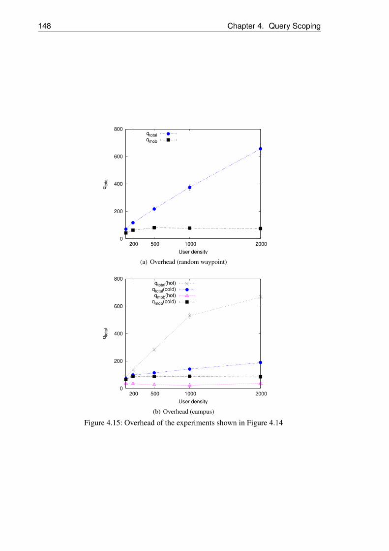
148 Chapter 4. Query Scoping
0
200
400
600
800
2000 1000 500 200
qto
tal
User density
qtotalqmob
(a) Overhead (random waypoint)
800
600
400
200
0 2000 1000 500 200
qto
tal
User density
qtotal(hot)qtotal(cold)qmob(hot)
qmob(cold)
(b) Overhead (campus)
Figure 4.15: Overhead of the experiments shown in Figure 4.14
4.7. Summary 149
then the protocol can do with much less queries by choosing a smallerinitial number of queries qinit.
Summing up, the above results are encouraging. In all our experiments,we could observe high rate of successful queries, that is, of objects beingfound. While the time until a reply can be obtained varies with user mo-bility and density, our conjecture – that most of the time an object will befound eventually – was confirmed. Moreover, we could show that even insettings with high positioning errors. or which rely solely on the observedcell identifier for localization, the total overhead for distributing an objectsearch query remains acceptably low.
Finally, in certain circumstances the system may even work reasonablywith very low participant densities which represent a hundredth of theexpected daytime population in an urban area. Based on these results,we assume that a similarly designed object localization system can beimplemented in practice.
4.7 Summary
In this chapter, we motivated and designed a comprehensive system formanaging and finding everyday items using mobile phones. We discussedthe architecture, design, and expected performance of this system, to-gether with a flexible query scoping algorithm that generates object searchheuristics from application data.
Our system makes use of an unconventional approach, as it relies on theparticipants’ mobility in order to cover an essential portion of the searchspace. We therefore spent significant effort on modeling and testing thecircumstances in which such an object search system would be used inthe large.
A prominent challenge of the presented object localization system is toselect a set of sensors that are likely to cover the phenomenon of inter-est, as a query cannot be distributed to all available sensors based on thescale of the system. This challenge was approached by a query scopingalgorithm that exports a generic interface for its configuration. Based onthe observation that every conceivable query scoping strategy would in-volve exploring history data stored by the system, the algorithm takes anannotated data model for an input, by which developers may parameterizealgorithm to implement arbitrary query scoping heuristics.
While different in its motivation and the underlying network model, theapproach repeats a pattern which re-alligns it with the previous chapters.

150 Chapter 4. Query Scoping
It uses a role-based configuration algorithm which exports a generic in-terface for setting up its behavior.

5 Conclusion
In the preceeding chapters, we have examined three rather heterogeneousapproaches to wireless sensor network configuration. In this final chapter,we summarize the presented contributions and discuss their limitations aswell as possible extensions.
5.1 Contributions
Each of the presented approaches allows programmers to express desiredconfiguration behaviour in a generic way. We summarize the taken ap-proaches in the following three sections.
5.1.1 Generic Role Assignment
Generic role assignment is a programmable service which supports devel-opers with network configuration tasks. Based on properties of the nodesand their network neighborhood, developers can specify conditions forassigning roles to sensor nodes. We argued that many network configura-tion problems can be considered instances of generic role assignment asthey can be expressed in terms of concise role assignment conditions.
Next to being expressive, the system is also efficient. In our evalua-tion, we showed that the communication costs incurred by generic roleassignment are proportional to the “hardness” of the specified problem.Moreover, we discussed how the overhead involved in implementing roleassignment problems is often comparable to specialized implementationsof these problems.
To help developers assess the quality of role assignment conditions (so-called role specifications), we provided a verification tool which can beused to perform offline analysis of a given role assignment problem. Inparticular, this tool can be used to detect erroneous specifications whichwill not generate any useful configuration when deployed to a network inoperation.
152 Chapter 5. Conclusion
5.1.2 Facility Location
The second contribution zooms in on a large subclass of role assignmentproblems which is concerned with selecting nodes that provide a serviceto client nodes in their network neighborhood.
This subclass of problems can be modeled by the facility location prob-lem. We therefore designed a distributed approximation algorithm for thefacility location problem which can be practically implemented on wire-less sensor nodes. Based on a set of parameters determining the cost in-volved in operating server nodes and the cost of communication betweenclients and their servers, the provided algorithm is able to find an optimaltrade-off between these two kinds of costs involved in network operation.
Using experiments, we could show that the presented algorithm findsnear-optimal solutions while depending only on local communicationconstrained to small network neighborhoods. Moreover, we found thata possible drawback of this algorithm, namely a high worst-case runtime,does rarely materialize in practice. In our experiments, the algorithm’sruntime is small and constant, that is, independent of the network size.
Apart from being close to optimal in the average case, the computedsolutions are guaranteed to be within a factor of 1.61 from the optimum,even in the worst-case. By integrating very good theoretical results (noteven a centralized polynomial algorithm can provide an approximationfactor better than 1.463) into a practicable local algorithm, the presentedwork can be considered to build a bridge between theory and practice.
5.1.3 Query Scoping
Our third contribution focused on a different subclass of configurationproblems, which involves selecting the subset of sensor nodes which ismost suitable for addressing a given sensing task.
The motivating application requires embedding sensors for detectingnearby objects into users’ mobile phones and makes use of the resultingsensing infrastructure to locate lost or misplaced objects. In order to beefficient, this system selects an appropriate subset of all sensors for han-dling a given user query on a misplaced object. In particular, the sensorselection is performed offline at the network base station avoiding com-municating with all sensors for each query.
The query scoping system has been custom tailored to its motivatingapplication: It selects sensors based on their utility in locating everydayitems which are of interest to users. In this context, we argued that the
5.2. Limitations 153
system may flexibly generate a large range of sensor selection heuristics,based on arbitrary data that is stored by the application (such as previousreports on an object).
In our evaluation, we compared the performance of query scoping torandom sensor selection strategies. Further, we evaluated the practica-bility of the mobile-phone-based object localization application itself. Inparticular, we examined various trade-offs involved in the design of user-centric sensing systems, and showed that adding sensors to only a smallfraction of the participants’ mobile phones already suffices for implement-ing the object localization application.
5.2 Limitations
As all three services summarized above provide generic interfaces fortheir parameterization, a set of common limitations can be associated toeach of them. The first is related to the expressiveness of the service in-terface. For example, each service has been custom-tailored to a certainclass of problems and does not allow for the implementation of functional-ity beyond this class. The second is related to the efficiency of the serviceimplementation when compared with custom-built specialized solutionsof similar problems. Last but not least, even if a service interface providesa high level of abstraction, developers must still perform a translation be-tween the desired application logic and the provided service interface, towhich we refer to as the interface’s semantic gap.
In the following three sections, we discuss the limitations of each con-tribution according to the above categories, as well as specific limitationswhich can be associated to each contribution.
5.2.1 Generic Role Assignment
Clearly, generic role assignment cannot be used to formulate every con-ceivable role assignment problem. Instead, its expressiveness is limited bydesign. For example, generic role assignment is specialized to symmet-ric problems, where each node follows the same set of rules. Moreover,the system focuses on configuration tasks whose role assignment condi-tions are formulated in terms of rather stable network properties. Whilenode properties may change over time, generic role assignment is onlyuseful if (on average) one role assignment iteration can conclude and the

154 Chapter 5. Conclusion
network is allowed to benefit from the computed configuration before thenext property changes necessitating re-configuration take place.
Moreover, generic role assignment is limited to configurations in whichgreedy assignment of roles according to the specification makes sense,that is, which do not require to observe certain global optimization cri-teria. For example, while it has been possible to guarantee near-optimalsolutions for the configuration tasks that can be modeled by the facilitylocation problem, such optimality guarantees are hard to achieve for allproblems specifiable by the generic role assignment system.
Further, we mentioned that the efficiency of the system is comparableto specialized implementations in many cases. However, one drawbackis that nodes propagate properties occurring in the role specification toall nodes within a local network neighborhood. Specialized implemen-tations, instead, may limit property propagation to nodes which benefitfrom the information.
Finally, generic role assignment’s semantic gap is hard to assess ade-quately and only tentative statements can be made. Boolean role assign-ment conditions are established concepts, which can readily capture thedeveloper’s logic (consider the clustering example, where cluster lead-ers are connected by gateways which function as bridges between them).What might diverge from developers’ intentions are the effects causedby unforeseen interdependencies between conditions for assigning differ-ent roles, which may in some cases result in non-terminating role assign-ment iterations. The role assignment solver, providing offline specifica-tion analysis, was built to overcome this concern.
A specific limitation of generic role assignment is that the speed ofits convergence to a stable set of roles is an open issue – although thisdrawback is not apparent in our experiments. A formal framework thatcategorizes classes of role-assignment problems based on their conver-gence properties (as has been done in [Wol94] for a synchronous execu-tion model and a constrained set of assignment rules) would be a valuableextension of our work. Because of the generality of the discussed rolespecifications, however, this remains a challenging open problem.
5.2.2 Distributed Facility Location
Analogous limitations exist for the provided facility location algorithms.Intuitively, their expresiveness is limited to configuration tasks that can bemodeled by the facility location problem. In particular, we considered the

5.2. Limitations 155
uncapacitated version of the problem, which does not set a limit on thenumber of clients per server node. Such limits, however, can be usefulin many applications. A possible extension of our algorithm thereforeis to address the capacitated facility location problem, as we describe inSection 5.3.2.
Moreover, our algorithms may suffer from drawbacks in efficiency whenapplied to problems which are “easier” than facility location. For exam-ple, the algorithms can be parameterized to compute a minimum dominat-ing set. However, specialized approaches which are based on assigningroles probabilistically [Lub85] are able to provide low approximation fac-tors involving fewer communication rounds.
Finally, the semantic gap of the facility location algorithms can be con-sidered low, as the connection and opening cost parameters may well rep-resent the energy spent by each of the two roles (client and server) withina given application.
A specific limitation of the described facility location algorithms is theirhigh worst-case runtime. Attempts to speed up facility location algo-rithms, however, should not compromise the (average-case) optimality ofthe obtained solution, as this would diminish the practical benefit of theapproach.
5.2.3 Query Scoping
Our query scoping approach provides a framework for determining theutility of sensors for answering user queries. While limited to the do-main of sensor selection, the expresiveness of this framework is relativelyhigh. Developers may issue arbitrary data models annotated with custom-implemented functions defining the relevance of the relations containedin the model.
Further, the efficiency of the approach has not been compared withspecialized implementations. This is because highly customized searchstrategies are not considered useful in the context of the object localiza-tion application.
Finally, we mentioned above that the semantic gap can be viewed asrelatively high compared to the previous two contributions. This is basedon the fact that the semantics of a given set of weight functions (assignedto relations of the data model) become only apparent when consideredtogether with the breadth-first search algorithm used for query scoping.Re-formulating the semantics of these functions (and of the relevance pa-

156 Chapter 5. Conclusion
rameters assigned to edges of the search graph) to denote probabilisticrelevance estimates (corresponding to the reciprocal of the currently usedcost-based estimates), could overcome this drawback.
Moreover, because the taken approach is application specific, it mightoccur that a given selection problem can be captured more effectively bya different specification technique (other than by annotated data models),for example, by directly defining a utility function that returns the rele-vance of a sensor with respect to a given sensing task.
5.3 Outlook
There are a number of ways in which each of our contributions couldbe improved. In the following three sections, we discuss potential areasof future work. Further, in Section 5.3.4 we provide an overview of thecore functionality addressed by this thesis, in order to provide guidelinesfor the design of a future, more comprehensive, network configurationservice.
5.3.1 Generic Role Assignment
Generic role assignment could be extended in various ways. The first isto allow nodes to take on multiple roles instead of just one. Implement-ing this extension would require changing the system’s semantics (cur-rently assigning the first role of the specification whose assignment con-ditions match) to instead assign all roles whose conditions match. Thesechanges would be particularly beneficial for applications, in which nodesperform different tasks concurrently. Note that such changed semanticscould easily be added to the existing system: The node protocol wouldassign all matching roles; the centralized solver would simply omit someconstraints.
A similar extension consists in maintaining the current role assignmentsemantics, but allow programmers to issue multiple role specificationswhich are all evaluated by the system at the same time. Given a set ofspecifications, the system would assign exactly one role from each ofthem, where each specification allows programmers to control a paral-lel set of node tasks. For example, nodes could adapt the behaviour oftheir routing components according to described clustering specification,while, at the same time, the mentioned coverage specification determineswhen to power up, or respectively shut down, the node’s sensing function-
5.3. Outlook 157
ality. Note that this extension can easily be implemented by re-executingthe existing local rule evaluation engine a couple of times for each speci-fied group of roles.
A third extension involves providing a more powerful local runtime en-vironment on the nodes. We have mentioned how additional operationsover local node properties (such a set intersection, substraction, or evencustom-implemented library functions) enable a range of more advancedrole specifications.
Finally, one could provide heuristics that attempt to realize certainglobal properties in the computed configurations. Most importantly, onecould optimize the use of certain roles (as already supported by the cen-tralized solver). Moreover, developers could be offered a feature, which(if enabled for a certain subset of roles) attempts to obtain configurationsin which the specified subsets of roles form a connected backbone.
5.3.2 Distributed Facility Location
The presented work on facility location could be continued on severalpaths. The algorithms we described could be made faster, possibly em-ploying a technique inspired by [MW05], in which stars are connected“fractionally” in small parallel steps and the obtained fractional solutionis rounded later.
Moreover, in wireless multi-hop networks two “harder” versions of thefacility location problem have particular applicability, for which, to ourknowledge, no distributed algorithms exist at all.
The first is capacitated facility location, which allows developers to im-pose a limit c on the clients which can be connected to one server node.This (harder) problem definition may require a significantly revised algo-rithm if a low approximation factor is desired. However, a slight revisionof the existing algorithms, in which nodes consider only the subset of starscontaining less than c clients, could already provide a useful approach.
The second is robust facility location, which requires every client to beredundantly connected by k facilities. Here, again, our algorithms couldalready provide useful heuristics if client nodes are allowed to connect tomore than one server (be part of k stars simultaneously) during algorithmexecution.
Finally, there are other promising applications of distributed facility lo-cation, which can be implemented by different parameterizations of theprovided facility location algorithms. For example, one could construct
158 Chapter 5. Conclusion
whole data aggregation trees, by re-executing the described algorithmsseveral times. In particular, one could parameterize consecutive execu-tions of the algorithms to select aggregators of different levels (that is, toconnect stars consisting of stars computed in the previous round) in eachexecution, and thus construct an efficient communication tree.
5.3.3 Query Scoping
The provided query scoping approach is application specific. One couldprovide an application-independent query scoping system by havingnodes perform statistics on their output over time. Once these statisticsare communicated to the network basestation, the basestation may directa query for a certain event of interest to sensors which, based on previousstatistics, are likely to observe such events.
5.3.4 A Comprehensive Configuration Framework
Apart from extensions to each individual service, an interesting path offuture work is to provide a comprehensive comfiguration service that ad-dresses functionality from all three contributions within a common frame-work. In this section, we are therefore interested in highlighting commonconcepts which re-appear in all our contributions, and can thus be ex-pected to be part of any future service that is concerned with networkconfiguration. In particular, we assume that a more advanced configura-tion service can approach all these concepts in a unified manner.
An aspect common to all our contributions on role-based configurationis that they implicitly provide functionality for grouping nodes. For ex-ample, generic role assignment forms groups in two distinct ways: Onthe one hand, nodes taking on the same role can be considered part of thesame group. On the other hand, roles which require that a given set ofnodes must be present in the local network neighborhood (for example anaggregator node which depends on a set of data sources) implicitly forma group consisting of the data sources and the chosen aggregator node.Facility location similarly associates nodes into clusters consisting of aserver and a set of clients. Query scoping groups nodes based on theirlikelihood to sense certain information.
Based on these observations, and the fact that similar functionality isinvolved in many related services [WSBC04, WM04, MP06, SFCB04,HKS+04] and programming frameworks [GGG05, NW04, BPRL05], we
5.3. Outlook 159
expect such composition and grouping of nodes to be part of any pro-gramming framework for wireless sensor networks. Therefore, in orderto provide guidelines for the design of a future configuration system, itseems worthwhile to zoom in further on the different aspects involved infunctionality for grouping nodes. Specifically, we found three such as-pects.
Composition. The first aspect involves combining services or data (suchas streams of some data type) from different nodes into more high-levelservices. For example, a cluster leader in a network performing fire de-tection could use its associated nodes to provide high-level reports on thecurrent status of a large portion of the observation area. A different exam-ple is smart farming where two sources of humidity and temperature sen-sors from the same area (possibly not collocated on the same node) mustbe combined to evaluate the likeliness of infection with certain fungi [Ins].Apart from composing streams of data, similarly, other services providedby network nodes (such as localization or time synchronization) couldbe composed into a more high level service. In summary, compositionfocuses on connecting services or data from different nodes into a morehigh-level bundle.
Exclusion. The second aspect involves granting nodes exclusive access tocertain sensing or processing resources, or ensuring that certain tasks areprocessed by a limited number of nodes (from a network neighborhood)only. Coverage problems are based on exclusion, as they prevent morethan one node from sensing the same area. In clustering approaches, typ-ically a single cluster leader makes exclusive use of the data provided byassociated slave nodes. The main purpose of exclusion aspects in wirelesssensor networks is energy efficiency. It attempts to avoid redundant datagathering or computation within certain areas of the network, when thetask can be performed sufficiently well by a single node or a small subsetof nodes. Applications that require a group of nodes to reach consensuson a certain value often elect one group leader to choose the value forthem, which is also a special case of exclusion functionality.
Selection. The third aspect involves selecting the most useful subset ofnodes based on the required task. Selection functionality can be straight-forward: The task may involve collecting data from a certain area (inwhich case sensors from this area are selected while the rest of the net-work remains inactive) or only from a given subject such as a certainbuilding or bridge (in which only sensors located near the subject are rel-

160 Chapter 5. Conclusion
evant for the sensing task). Alternatively, more involved methods for se-lecting nodes can be provided, for example, the sensor ranking performedby our query scoping approach. Note that selection can be performed off-line at the network base station, as done by our query scoping system, aswell as online inside of the network, where the nodes themselves computewhether they should be selected (as could be implemented by generic roleassignment).
Note the orthogonality of the three aspects above. Composition wiresthe different sensors together into compound entities. Exclusion avoidsthat certain data or tasks are processed redundantly by multiple entities.Selection chooses the most useful entities for a given sensing task.
The expressiveness of generic role assignment can be explained by thefact that it integrates all three aspects. It implements composition by al-lowing to specify conditions requiring that nodes with certain properties(or roles) should be present in the network neighborhood. It also ad-dresses exclusion as it allows to require that no other nodes with certainproperties should be present. Finally, the role abstraction can be used as ameans for online selection of nodes by enabling developers to include se-lection conditions in terms of local node node properties, such as a node’slocation, its current sensor readings, or its battery status, into role assign-ment conditions.
Facility location achieves specific intertwined composition and exclu-sion functionality involved in the clustering problem. While it composesgroups of nodes into stars, at the same time it ensures that the star’s clientsare exclusively connected by the facility rooting the star (that is, that starsdo not overlap and therefore information from clients is not processed re-dundantly). Finally, query scoping expands on the orthogonal selectionproblem, an aspect that is not present in the facility location system.
A future configuration service would need to integrate composition, ex-clusion and selection into a common programming framework. Whilegeneric role assignment has performed such integration, a future sys-tem might benefit from providing programmers with more explicit controlover the above aspects and the interaction between them.
A promising candidate to address composition are graphs which statethe desired composed structure (such as task graphs in ATaG [BPRL05]).Constraining these graphs to have the form of trees would allow for moreefficient implementation of the configuration runtime and still capturemost functionality of the composition aspect. Note that facility locationaddresses composition for graphs which have the form of stars.
5.4. Concluding Remarks 161
Extensions regarding exclusion would allow developers to define ad-ditional entities (such as services, node groups or geographic areas) andconstraints on the access to them by other entities. Note that – just likethe accessed entities – the accessing entities do not need to be nodes.
Additional support for selection might include allowing developers toplug in functions that compute a ranking of nodes, either online basedon certain local properties, such as the number of clients connected to aclusterhead or the nodes’ battery level, or offline based on statistics onlocal properties which have been propagated to the network base station.Automated mechanisms for efficient online selection according to a givenranking function, and for the propagation of statistics to the network basestation in order to perform offline selection based on the same functionlater on, may be another interesting direction to pursue in a future system.
5.4 Concluding Remarks
In this thesis, we approached role-based configuration problems fromthree distinct points of view which were founded on different applica-tion domains. Due to the wide range of applications which require role-based configuration, we believe that we touched upon core challengeswhich will manifest themselves in every network configuration problem.By facing these challenges in a variety of ways, we provide a more com-prehensive understanding of potential solutions – by which we hope tofacilitate the design of future systems concerned with the configuration ofwireless sensor networks.

162 Chapter 5. Conclusion

Bibliography
[AAC+00] Harold Abelson, Don Allen, Daniel Coore, Chris Hanson,George Homsy, Jr. Thomas F. Knight, Radhika Nagpal, ErikRauch, Gerald Jay Sussman, and Ron Weiss. AmorphousComputing. Communications of the ACM, 43(5):74–82,March 2000.
[ABC+04] T. Abdelzaher, B. Blum, Q. Cao, Y. Chen, D. Evans,J. George, S. George, L. Gu, T. He, S. Krishnamurthy,L. Luo, S. Son, J. A. Stankovic, R. Stoleru, andA. Wood. EnviroTrack: Towards an Environmental Com-puting Paradigm for Distributed Sensor Networks. InProceedings of the 24th International Conference on Dis-tributed Computing Systems (ICDCS’04), Tokyo, Japan,March 2004.
[ASSC02] I. F. Akyildiz, W. Su, Y. Sankarasubramaniam, andE. Cayirci. Wireless Sensor Networks: A Survey. ComputerNetworks, 38(4):393–422, March 2002.
[Bar04] Rimon Barr. An efficient, unifying approach to simulationusing virtual machines. PhD thesis, Cornell University, May2004.
[BB03] Boris Jan Bonfils and Philippe Bonnet. Adaptive and decen-tralized operator placement for in-network query processing.In Proceedings of the 2nd International Workshop on Infor-mation Processing in Sensor Networks (IPSN’03), pages 47–62, April 2003.
[BBH+04] Gaetano Borriello, Waylon Brunette, Matthew Hall, CarlHartung, and Cameron Tangney. Reminding about taggedobjects using passive RFIDs. In Proceedings of the 6thInternational Conference on Ubiquitous Computing (Ubi-Comp’04), Nottingham, England, September 2004.

164 Bibliography
[BC02] Manish Bhardwaj and Anantha P. Chandrakasan. Bound-ing the lifetime of sensor networks via optimal role assign-ments. In Proceedings of the 21st Annual Joint Conferenceof the IEEE Computer and Communications Societies (IN-FOCOM’02), New York, NY, USA, 2002.
[BEH+06] J. Burke, D. Estrin, M. Hansen, A. Parker, N. Ramanathan,S. Reddy, and M. B. Srivastava. Participatory sensing. InSENSYS’06 Workshop on World-Sensor-Web: Mobile De-vice Centric Sensor Networks and Applications (WSW’06),Boulder, CO, USA, November 2006.
[BGS01] Philippe Bonnet, Johannes Gehrke, and Praveen Seshadri.Towards sensor database systems. In Proceedings of the Sec-ond International Conference on Mobile Data Management,Hong Kong, China, January 2001.
[BIK+04] Cristian Borcea, Chalermek Intanagonwiwat, Porlin Kang,Ulrich Kremer, and Liviu Iftode. Spatial programming usingsmart messages: Design and implementation. In Proceed-ings of the 24th International Conference on DistributedComputing Systems (ICDCS’04), pages 690–699, Tokyo,Japan, March 2004. IEEE Computer Society.
[BKG06] Fang Bian, David Kempe, and Ramesh Govindan. Utilitybased sensor selection. In Proceedings of the 5th Interna-tional Conference on Information Processing in Sensor Net-works (IPSN’06), pages 11–18, Nashville, Tennessee, USA,April 2006. ACM Press.
[BKM+04] Jan Beutel, Oliver Kasten, Friedemann Mattern, Kay Römer,Lothar Thiele, and Frank Siegemund. Prototyping SensorNetwork Applications with BTnodes. In Proceedings ofthe 1st European Workshop on Wireless Sensor Networks(EWSN’04), Berlin, Germany, January 2004.
[BL06] Philipp Bolliger and Marc Langheinrich. Distributed persis-tence for limited devices. In System Support for UbiquitousComputing Workshop (UbiSys’06) at UbiComp’06, OrangeCounty, CA, USA, September 2006.
Bibliography 165
[BLM05] Philippe Bonnet, Martin Leopold, and Jan Madsen. TheHogthrob Probject. http://www.hogthrob.dk/,2005.
[BMP04] Stefano Basagni, Michele Mastrogiovanni, and Chiara Petri-oli. A performance comparison of protocols for clusteringand backbone formation in large scale ad hoc networks. InProceedings of the 1st IEEE International Conference onMobile Ad-hoc and Sensor Systems (MASS’04), 2004.
[Bok81] Shahid H. Bokhari. A shortest tree algorithm for optimalassignments across space and time in a distributed processorsystem. IEEE Trans. on Software Engineering, 7(6):583–589, November 1981.
[Bok87] Shahid H. Bokhari. Assignment problems in parallel anddistributed computing. Kluwer Academic Publishers, Nor-well, MA, USA, 1987.
[BP98] Sergey Brin and Lawrence Page. The anatomy of a large-scale hypertextual web search engine. In Proceedings of the7th International World Wide Web Conference (WWW’98),pages 107–117, Brisbane, Australia, April 1998. ElsevierScience Publishers B. V.
[BPRL05] Amol Bakshi, Viktor K. Prasanna, Jim Reich, and DanielLarner. The Abstract Task Graph: a methodology forarchitecture-independent programming of networked sensorsystems. In Proceedings of the 2005 workshop on end-to-end, sense-and-respond systems, applications and services(EESR’05), pages 19–24, Seattle, WA, USA, 2005. USENIXAssociation.
[BS03] Athanassios Boulis and Mani B. Srivastava. Design and im-plementation of a framework for efficient and programmablesensor networks. In Proceedings of the 1st InternationalConference on Mobile Systems, Applications, and Services(MOBISYS’03), San Francisco, CA, USA, May 2003.
[BTn06] BTnodes. www.btnode.ethz.ch, 2006.
166 Bibliography
[CC04] SmartRF CC1000 Datasheet (rev. 2.2). Chipcon AS, April2004. www.chipcon.com/files/CC1000_Data_Sheet_2_2.pdf.
[CEPS05] Fabian Chudak, Thomas Erlebach, Alessandro Panconesi,and Mauro Sozio. Primal-dual distributed algorithms forcovering and facility location problems. UnpublishedManuscript, 2005.
[CGG+05] Carlo Curino, Matteo Giani, Marco Giorgetta, AlessandroGiusti, Amy L. Murphy, and Gian Pietro Picco. Mobiledata collection in sensor networks: The TINYLIME Middle-ware. Elsevier Pervasive and Mobile Computing Journal,4(1):446–469, December 2005.
[CHP+04] P. Corke, S. Hrabar, R. Peterson, D. Rus, S. Saripalli, andG. Sukhatme. Autonomous deployment and repair of a sen-sor network using an unmanned aerial vehicle. In Proceed-ings of IEEE International Conference on Robotics and Au-tomation (ICRA’04), pages 3602–3608, May 2004.
[Cle96] Scott H. Clearwater, editor. Market-based control: aparadigm for distributed resource allocation. World Sci-entific Publishing Co., Inc., River Edge, NJ, USA, 1996.
[CPX] CPLEX ILP solver. www.ilog.com/products/cplex/.
[DGV04] Adam Dunkels, Bjorn Gronvall, and Thiemo Voigt. Contiki- a lightweight and flexible operating system for tiny net-worked sensors. In Proceedings of the 29th IEEE Interna-tional Conference on Local Computer Networks (LCN’04),Washington, DC, USA, 2004.
[DKB03] Christian Decker, Uwe Kubach, and Michael Beigl. Re-vealing the retail black box by interaction sensing. In 3rdInternational Workshop on Smart Appliances and WearableComputing (SAWC’03) at ICDCS’03, Providence, RI, USA,May 2003.
[EAL+06] Shane B. Eisenman, Gahng-Seop Ahn, Nicholas D. Lane,Emiliano Miluzzo, Ronald A. Peterson, and Andrew T.Campbell. MetroSense project: People-centric sensingat scale. In SENSYS’06 Workshop on World-Sensor-Web:
Bibliography 167
Mobile Device Centric Sensor Networks and Applications(WSW’06), Boulder, CO, USA, November 2006.
[EGT05] Andreas Eisenblätter, Hans-Florian Geerdes, and UlrichTürke. Public UMTS radio network evaluation and planningscenarios. International Journal on Mobile Network Designand Innovation, 1(1):40–53, 2005.
[EHJ04] Stephan J. Engberg, Morten B. Harning, and Christian D.Jensen. Zero-knowledge device authentication: Privacy &security enhanced RFID preserving business value and con-sumer convenience. In Proceedings of the 2nd Annual Con-ference on Privacy, Security and Trust (PST’04), October2004.
[ETS98] ETSI. Selection procedures for the choice of radio transmis-sion technologies of the UMTS. Technical Report 3.2.0, Eu-ropean Telecommunications Standards Institute, April 1998.
[FBMK07] Christian Frank, Philipp Bolliger, Friedemann Mattern, andWolfgang Kellerer. The Sensor Internet at work: Locat-ing objects using mobile phones. Submitted for publication,2007.
[FBRK07] Christian Frank, Philipp Bolliger, Christof Roduner, andWolfgang Kellerer. Objects calling home: Locating objectsusing mobile phones. In Proceedings of the 5th Interna-tional Conference on Pervasive Computing (Pervasive’07),Toronto, ON, Canada, May 2007.
[FCX+03] Lucio Ferreira, Luis M. Correia, David Xavier, Allen Vas-concelos, and Erik Fledderus. Deliverable d1.4: Final reporton traffic estimation and services characterisation. TechnicalReport IST-2000-28088, Momentum Project, 2003.
[Fei98] Uriel Feige. A threshold of lnn for approximating set cover.Journal of the ACM, 45(4), 1998.
[FR05] Christian Frank and Kay Römer. Algorithms for genericrole assignment in wireless sensor networks. In Proceed-ings of the 3rd International Conference on Embedded Net-worked Sensor Systems (SENSYS’05), San Diego, CA, USA,November 2005.
168 Bibliography
[FR06] Christian Frank and Kay Römer. Solving generic role as-signment exactly. In Proceedings of the 14th InternationalWorkshop on Parallel and Distributed Real-Time Systems(WPDRTS’06), Island of Rhodes, Greece, April 2006.
[FR07] Christian Frank and Kay Römer. Distributed facility locationalgorithms for flexible configuration of wireless sensor net-works. In Proceedings of the 3rd International Conferenceon Distributed Computing in Sensor Systems (DCOSS’07),Santa Fe, NM, USA, June 2007.
[Fra07] Christian Frank. Facility location. In Dorothea Wagner andRoger Wattenhofer, editors, Algorithms for Sensor and AdHoc Networks. Springer-Verlag, 2007.
[FRB+07] Christian Frank, Christof Roduner, Philipp Bolliger, ChieNoda, and Wolfgang Kellerer. A service architecture formonitoring physical objects using mobile phones. In Pro-ceedings of the 7th International Workshop on Applicationsand Services in Wireless Networks (ASWN’07), Santander,Spain, May 2007.
[FRNK06] Christian Frank, Christof Roduner, Chie Noda, and Wolf-gang Kellerer. Query scoping for the Sensor Internet. InProceedings of the IEEE International Conference on Per-vasive Services (ICPS’06), Lyon, France, June 2006.
[GEG+03] Benjamin Greenstein, Deborah Estrin, Ramesh Govindan,Sylvia Ratnasamy, and Scott Shenker. DIFS: a distributedindex for features in sensor networks. In Proceedings of the1st IEEE International Workshop on Sensor Network Proto-cols and Applications (SNPA’03), pages 163–173, Anchor-age, AK, USA, May 2003.
[GGG05] Ramakrishna Gummadi, Omprakash Gnawali, and RameshGovindan. Macro-programming wireless sensor networksusing Kairos. In Proceedings of the 1st InternationalConference on Distributed Computing in Sensor Systems(DCOSS’05), Marina del Rey, CA, USA, June 2005.
[GGJ+06] Omprakash Gnawali, Ben Greenstein, Ki-Young Jang, Au-gust Joki, Jeongyeup Paek, Marcos Vieira, Deborah Estrin,
Bibliography 169
Ramesh Govindan, and Eddie Kohler. The TENET archi-tecture for tiered sensor networks. In Proceedings of the 4thInternational Conference on Embedded Networked SensorSystems (SENSYS’06), Boulder, CO, USA, November 2006.
[GK99] Sudipto Guha and Samir Khuller. Greedy strikes back: Im-proved facility location algorithms. Journal of Algorithms,31:228–248, 1999.
[GKK+03] Phillip B. Gibbons, Brad Karp, Yan Ke, Suman Nath, andSrinivasan Seshan. IrisNet: An architecture for a worldwidesensor web. IEEE Pervasive Computing, 2(4), 2003.
[GLS06] Joachim Gehweiler, Christiane Lammersen, and ChristianSohler. A distributed O(1)-approximation algorithm for theuniform facility location problem. In Proceedings of the18th Annual ACM Symposium on Parallel Algorithms andArchitectures (SPAA’06), Cambridge, MA, USA, 2006.
[GZDG05] Himanshu Gupta, Zongheng Zhou, Samir R. Das, andQuinyi Gu. Connected sensor cover: Self-organization ofsensor networks for efficient query execution. ACM/IEEETransactions on Networking, 2005.
[HCB00] Wendi R. Heinzelman, Anantha Chandrakasan, and HariBalakrishnan. Energy-efficient communication protocolfor wireless microsensor networks. In Proceedings of the33rd Hawaii International Conference on System Sciences(HICSS’00), 2000.
[HKS+04] Tian He, Suda Krishnamurthy, John A. Stankovic, Tarek F.Abdelzaher, Liqian Luo, Radu Stoleru, Ting Yan, Lin Gu,Jonathan Hui, and Bruce Krogh. An energy-efficient surveil-lance system using wireless sensor networks. In In Proceed-ings of Second International Conference on Mobile Systems,Applications, and Services (MobiSys), 2004.
[HKS+05] Chih-Chieh Han, Ram Kumar, Roy Shea, Eddie Kohler, andMani B. Srivastava. A dynamic operating system for sen-sor nodes. In Proceedings of the 3rd International Confer-ence on Mobile Systems, Applications, and Services (MO-BISYS’05), pages 163–176, Seattle, WA, USA, June 2005.

170 Bibliography
[HMCP04] Wendi R. Heinzelman, Amy L. Murphy, Hervaldo S. Car-valho, and Mark A. Perillo. Middleware to support sensornetwork applications. IEEE Network, pages 6–14, January2004.
[Hoc82] Dorit S. Hochbaum. Heuristics for the fixed cost me-dian problem. Mathematical Programming, 22(1):148–162,1982.
[IB05] Volkan Isler and Ruzena Bajcsy. The sensor selection prob-lem for bounded uncertainty sensing models. In Proceedingsof the 4th International Symposium on Information Process-ing in Sensor Networks (IPSN’05), Los Angeles, CA, USA,April 2005.
[IEGH02] Chalermek Intanagonwiwat, Deborah Estrin, RameshGovindan, and John Heidemann. Impact of network den-sity on data aggregation in wireless sensor networks. InProceedings of the 22nd International Conference on Dis-tributed Computing Systems (ICDCS’02), Vienna, Austria,July 2002. IEEE Computer Society.
[IGE00] Chalermek Intanagonwiwat, Ramesh Govindan, and Deb-orah Estrin. Directed Diffusion: A Scalable and RobustCommunication Paradigm for Sensor Networks. In Proceed-ings of the 6th Annual International Conference on MobileComputing and Networking (MOBICOM’00), Boston, MA,USA, August 2000. ACM Press.
[Ins] Pessl Instruments. Potato and onion disease models. www.metos.at/diseasemodels/Potato.pdf.
[JMM+03] Kamal Jain, Mohammad Mahdian, Evangelos Markakis,Amin Saberi, and Vijai V. Vazirani. Greedy facility locationalgorithms analyzed using dual fitting with factor-revealingLP. Journal of the ACM, 50:795–824, November 2003.
[JOW+02] Philo Juang, Hidekazu Oki, Yong Wang, MargaretMartonosi, Li Shiuan Peh, and Daniel Rubenstein. Energy-efficient computing for wildlife tracking: design tradeoffsand early experiences with zebranet. ACM SIGPLAN No-tices, 37(10):96–107, 2002.

Bibliography 171
[JV99] Kamal Jain and Vijai V. Vazirani. Primal-dual approxima-tion algorithms for metric facility location and k-medianproblems. In Proceedings of the 40th Annual IEEE Sym-posium on Foundations of Computer Science (FOCS’99),pages 2–13, October 1999.
[KG02] Taek Jin Kwon and Mario Gerla. Efficient flooding withpassive clustering (PC) in ad hoc networks. Computer Com-munication Review, 32(1):44–56, January 2002.
[KHHK04] Andreas Köpke, Vlado Handziski, Jan-Hinrich Hauer, andHolger Karl. Structuring the information flow in component-based protocol implementations for wireless sensor nodes.In Proceedings of the Work-in-Progress Session of the1st European Workshop on Wireless Sensor Networks(EWSN’04), pages 41–45, Berlin, Germany, January 2004.
[KKK06] Minkyong Kim, David Kotz, and Songkuk Kim. Extract-ing a mobility model from real user traces. In Proceedingsof the 25th Annual Joint Conference of the IEEE Computerand Communications Societies (INFOCOM’06), Barcelona,Spain, April 2006.
[Koc05] Thorsten Koch. ZIMPL (Zuse Institute Mathematical Pro-gramming Language) User Guide, February 2005.
[KR05] Oliver Kasten and Kay Römer. Beyond event handlers: Pro-gramming wireless sensors with attributed state machines.In Proceedings of the 4th International Symposium on In-formation Processing in Sensor Networks (IPSN’05), pages45–52, Los Angeles, USA, April 2005.
[KSG03] Manish Kochhal, Loren Schwiebert, and Sandeep Gupta.Role-based hierarchical self organization for wireless ad hocsensor networks. In Proceedings of the 2nd ACM Interna-tional Workshop on Wireless Sensor Networks and Applica-tions (WSNA’03), San Diego, CA, USA, 2003.
[KSW05] Denis Krivitski, Assaf Schuster, and Ran Wolff. A localfacility location algorithm for sensor networks. In Pro-ceedings of the 1st International Conference on DistributedComputing in Sensor Systems (DCOSS’05), Marina del Rey,CA, USA, June 2005.

172 Bibliography
[KV02] Bernhard Korte and Jens Vygen. Colouring, chapter 16.2,pages 367–373. Springer-Verlag, 2nd edition, 2002.
[KW03] Fabian Kuhn and Roger Wattenhofer. Constant-time dis-tributed dominating set approximation. In Proceedingsof the 22nd ACM Symposium on Principles of DistributedComputing (PODC’03), July 2003.
[KW05] Holger Karl and Andreas Willig. Protocols and Architec-tures for Wireless Sensor Networks. Wiley, May 2005.
[LAHS06] Liqian Luo, Tarek F. Abdelzaher, Tian He, and John A.Stankovic. Envirosuite: An environmentally immersive pro-gramming framework for sensor networks. ACM Trans-actions on Embedded Computing Systems, 5(3):543–576,2006.
[LC02] Philip Levis and David Culler. Maté: A tiny virtual machinefor sensor networks. Operating Systems Review, 36(5):85 –95, December 2002.
[LMFJ+04] Konrad Lorincz, David J. Malan, Thaddeus R.F. Fulford-Jones, Alan Nawoj, Antony Clavel, Victor Shnayder, Geof-frey Mainland, and Matt Welsh. Sensor networks for emer-gency response: Challenges and opportunities. IEEE Perva-sive Computing, 3(4):16–23, October 2004.
[LMMR05] Andreas Lachenmann, Pedro José Marrón, Daniel Minder,and Kurt Rothermel. An analysis of cross-layer interactionsin sensor network applications. In Proceedings of the 2ndInternational Conference on Intelligent Sensors, Sensor Net-works & Information Processing (ISSNIP’05), pages 121–126, December 2005.
[LPCS04] Philip Levis, Neil Patel, David Culler, and Scott Shenker.Trickle: A self-regulating algorithm for code propagationand maintenance in wireless sensor networks. In Proceed-ings of the First Symposium on Networked System Designand Implementation (NSDI’04), San Francisco, CA, USA,March 2004.
[LRT04] Kari Laasonen, Mika Raento, and Hannu Toivonen. Adap-tive on-device location recognition. In Proceedings of the

Bibliography 173
2nd International Conference on Pervasive Computing (Per-vasive’04), Vienna, Austria, April 2004.
[LRW+05] Hongzhou Liu, Tom Roeder, Kevin Walsh, Rimon Barr, andEmin Gun Sirer. Design and implementation of a singlesystem image operating system for ad hoc networks. InProceedings of the 3rd International Conference on MobileSystems, Applications, and Services (MOBISYS’05), Seattle,WA, USA, June 2005.
[LSS03] Shuoqi Li, Sang H. Son, and John A. Stankovic. Event de-tection services using data service middleware in distributedsensor networks. In Proceedings of the 2nd InternationalWorkshop on Information Processing in Sensor Networks(IPSN’03), volume 2634 of Lecture Notes in Computer Sci-ence, pages 502 – 517, Palo Alto, CA, USA, April 2003.Springer-Verlag.
[LSZM04] Ting Liu, Christopher M. Sadler, Pei Zhang, and MargaretMartonosi. Implementing software on resource-constrainedmobile sensors: Experiences with Impala and ZebraNet. InProceedings of the 2nd International Conference on MobileSystems, Applications, and Services (MOBISYS’04), Boston,MA, USA, June 2004. ACM Press.
[Lub85] Michael Luby. A simple parallel algorithm for the maximalindependent set problem. In Proceedings of the 17th An-nual ACM Symposium on Theory of Computing (STOC’85),pages 1–10, New York, NY, USA, May 1985. ACM Press.
[LV05] Jean-Yves Le Boudec and Milan Vojnovic. Perfect simula-tion and stationarity of a class of mobility models. In Pro-ceedings of the 24th Annual Joint Conference of the IEEEComputer and Communications Societies (INFOCOM’05),Miami, FL, USA, March 2005.
[Lyn81] Nancy Lynch. Upper bounds for static resource allocationin a distributed system. Journal of Computer and SystemSciences, 23(2):254–278, 1981.
[MFHH02] Samuel Madden, Michael J. Franklin, Joseph M. Heller-stein, and Wei Hong. TAG: a Tiny AGgregation Service for

174 Bibliography
Ad-Hoc Sensor Networks. In Proceedings of the 5th Sym-posium on Operating Systems Design and Implementation(OSDI’02), Boston, MA, USA, December 2002.
[MFHH03] Samuel Madden, Michael J. Franklin, Joseph M. Hellerstein,and Wei Hong. The design of an acquisitional query proces-sor for sensor networks. In Proceedings of the 22th Inter-national Conference on Management of Data / Principlesof Database Systems (SIGMOD/PODS’03), pages 491–502,San Diego, CA, USA, June 2003.
[MFHH05] Samuel Madden, Michael J. Franklin, Joseph M. Hellerstein,and Wei Hong. TinyDB: An acquisitional query processingsystem for sensor networks. ACM Transactions on DatabaseSystems, 30(1):122–173, 2005.
[MKPS01] Seapahn Meguerdichian, Farinaz Koushanfar, MiodragPotkonjak, and Mani B. Srivastava. Coverage problemsin wireless ad-hoc sensor networks. In Proceedings ofthe 20th Annual Joint Conference of the IEEE Computerand Communications Societies (INFOCOM’01), volume 3,pages 1380–1387, 2001.
[MLM+05] Pedro José Marrón, Andreas Lachenmann, Daniel Minder,Jörg Hähner, Robert Sauter, and Kurt Rothermel. Tiny-Cubus: A flexible and adaptive framework for sensor net-works. In Proceedings of the 2nd European Workshop onWireless Sensor Networks (EWSN’05), January 2005.
[Mom06] Momentum. Models and simulation for network planningand control of UMTS. momentum.zib.de/data.php,May 2006.
[Mos07] Thomas Moscibroda. Clustering. In Dorothea Wagner andRoger Wattenhofer, editors, Algorithms for Sensor and AdHoc Networks. Springer-Verlag, 2007.
[MP06] Luca Mottola and Gian Pietro Picco. Logical Neighbor-hoods: A programming abstraction for wireless sensor net-works. In Proceedings of the 2nd International Conferenceon Distributed Computing in Sensor Systems (DCOSS’06),pages 150–167, San Francisco, CA, USA, June 2006.
Bibliography 175
[MPS+02] Alan Mainwaring, Joseph Polastre, Robert Szewczyk, DavidCuller, and John Anderson. Wireless sensor networks forhabitat monitoring. In Proceedings of the 1st ACM Interna-tional Workshop on Wireless Sensor Networks and Applica-tions (WSNA’02), Atlanta, GA, USA, September 2002.
[MPW05] Geoffrey Mainland, David C. Parkes, and Matt Welsh. De-centralized, adaptive resource allocation for sensor net-works. In Proceedings of the Second Symposium onNetworked System Design and Implementation (NSDI’05),Boston, MA, USA, May 2005.
[MW05] Thomas Moscibroda and Roger Wattenhofer. Facility lo-cation: Distributed approximation. In Proceedings of the24th ACM Symposium on Principles of Distributed Comput-ing (PODC’05), pages 108–117, 2005.
[MYZ02] Mohammad Mahdian, Yinyu Ye, and Jiawei Zhang. Im-proved approximation algorithms for metric facility locationproblems. In Proceedings of the 5th International Workshopon Approximation Algorithms for Combinatorial Optimiza-tion (APPROX’02), Rome, Italy, September 2002.
[NAW05] Ryan Newton, Arvind, and Matt Welsh. Building upto macroprogramming: an intermediate language for sen-sor networks. In Proceedings of the 4th InternationalSymposium on Information Processing in Sensor Networks(IPSN’05), Los Angeles, CA, USA, 2005.
[NMW07] Ryan Newton, Greg Morrisett, and Matt Welsh. The Regi-ment macroprogramming system. In Proceedings of the 6thInternational Conference on Information Processing in Sen-sor Networks (IPSN’07), pages 489–498, Cambridge, MA,USA, 2007.
[NW04] Ryan Newton and Matt Welsh. Region streams: functionalmacroprogramming for sensor networks. In Proceeedingsof the 1st International Workshop on Data Management forSensor Networks (DMSN’04), pages 78–87, Toronto, ON,Canada, 2004.
[PHC04] Joseph Polastre, Jason Hill, and David Culler. Versatile lowpower media access for wireless sensor networks. In Pro-
176 Bibliography
ceedings of the 2nd International Conference on Embed-ded Networked Sensor Systems (SENSYS’04), pages 95–107,Baltimore, MD, USA, 2004.
[PLS+06] Peter Pietzuch, Jonathan Ledlie, Jeffrey Shneidman, MemaRoussopoulos, Matt Welsh, and Margo Seltzer. Network-aware operator placement for stream-processing systems. InProceedings of the 22nd International Conference on DataEngineering (ICDE’06), Atlanta, GA, USA, April 2006.
[Ram99] Subramanian Ramanathan. A unified framework and algo-rithm for channel assignment in wireless networks. WirelessNetworks, 5(2):81–94, 1999.
[RF 06] RF Code, Inc. MantisTM active RFID tags 433 MHzdata sheet. www.rfcode.com/data_sheets/433_mantis_tags.pdf, 2006.
[RFMB04] Kay Römer, Christian Frank, Pedro José Marrón, and Chris-tian Becker. Generic role assignment for wireless sensor net-works. In Proceedings of the 11th ACM SIGOPS EuropeanWorkshop, Leuven, Belgium, September 2004.
[RN95] Stuart Russell and Peter Norvig. Artificial Intelligence: Amodern approach, chapter 3, pages 75–76. Prentice Hall,1995.
[SAGP00] Katayoun Sohrabi, Vishal Ailawadhi, Jay Gao, and Gre-gory J. Pottie. Protocols for self organization of a wirelesssensor network. Personal Communication Magazine, 7:16–27, 2000.
[San05] Paolo Santi. Topology Control in Wireless Ad Hoc and Sen-sor Networks. Wiley, 2005.
[Sen07] SensorPlanet. www.sensorplanet.org, 2007.
[SFCB04] Jan Steffan, Ludger Fiege, Mariano Cilia, and AlejandroBuchmann. Scoping in wireless sensor networks: a posi-tion paper. In Proceedings of the 2nd Workshop on Middle-ware for Pervasive and Ad-hoc Computing, pages 167–171,Toronto, Ontario, Canada, 2004. ACM Press.

Bibliography 177
[SHK+05] Hirobumi Shimizu, Osamu Hanzawa, Kenichiro Kanehana,Hiroki Saito, Niwat Thepvilojanapong, Kaoru Sezaki, andYoshito Tobe. Association management between everydayobjects and personal devices for passengers in urban areas.Demonstration Abstract in Adjunct Proceedings of Perva-sive’05, Munich, Germany, May 2005.
[SK00] Lakshminarayanan Subramanian and Randy H. Katz. Anarchitecture for building self-configurable systems. In Pro-ceedings of the 1st ACM International Symposium on Mo-bile Ad Hoc Networking and Computing (MOBIHOC’01),Boston, MA, USA, August 2000.
[SP01] Sasa Slijepcevic and Miodrag Potkonjak. Power efficientorganization of wireless sensor networks. In Proceedingsof the IEEE International Conference on Communications(ICC’01), Helsinki, Finland, June 2001.
[Sto77] Harold S. Stone. Multiprocessor scheduling with the aid ofnetwork flow algorithms. IEEE Transactions on SoftwareEngineering, SE-3(1):83–93, Jan 1977.
[TG03] Di Tian and Nicolas D. Georganas. A node schedulingscheme for energy conservation in large wireless sensor net-works. Wireless Communications and Mobile Computing,3(2):271–290, 2003.
[Tmo05] Tmote Sky datasheet 1.0.2. www.moteiv.com, December2005.
[TOS] TinyOS. webs.cs.berkeley.edu/tos/.
[TP05] Dirk Trossen and Dana Pavel. Building a ubiquitous plat-form for remote sensing using smartphones. In Proceed-ings of the 2nd Annual International Conference on Mobileand Ubiquitous Systems: Networks and Services (MobiQui-tous’05), pages 485–489, July 2005.
[TPS+05] Gilman Tolle, Joseph Polastre, Robert Szewczyk, DavidCuller, Neil Turner, Kevin Tu, Stephen Burgess, Todd Daw-son, Phil Buonadonna, David Gay, and Wei Hong. A macro-scope in the redwoods. In Proceedings of the 3rd Interna-
178 Bibliography
tional Conference on Embedded Networked Sensor Systems(SENSYS’05), San Diego, CA, USA, November 2005.
[TWS06] Kirsten Terfloth, Georg Wittenburg, and Jochen H. Schiller.FACTS - a rule-based middleware architecture for wirelesssensor networks. In Proceedings of the 1st InternationalConference on Communication Systems Software and Mid-dleware (COMSWARE’06), New Delhi, India, 2006.
[UWMG05] Andreas Ulbrich, Torben Weis, Gero Mühl, and Kurt Geihs.Application Development for Actuator and Sensor Net-works. In GI Workshop on Sensor Networks, ETH Zurich,Switzerland, March 2005.
[Vaz03] Vijai V. Vazirani. Approximation Algorithms. Springer-Verlag, 2003.
[vDL03] Tijs van Dam and Koen Langendoen. An adaptive energy-efficient mac protocol for wireless sensor networks. In Pro-ceedings of the 1st International Conference on EmbeddedNetworked Sensor Systems (SENSYS’03), Los Angeles, CA,USA, November 2003.
[Vyg05] Jens Vygen. Approximation algorithms for facility locationproblems. Technical Report 05950-OR, Research Institutefor Discrete Mathematics, University of Bonn, 2005.
[WAJR+05] Geoffrey Werner-Allen, Jeff Johnson, Mario Ruiz, JonathanLees, and Matt Welsh. Monitoring volcanic eruptions witha wireless sensor network. In Proceedings of the 2nd Eu-ropean Workshop on Wireless Sensor Networks (EWSN’05),Istanbul, Turkey, January 2005.
[WC01] Alec Woo and David Culler. A transmission control schemefor media access in sensor networks. In Proceedings of the7th Annual International Conference on Mobile Computingand Networking (MOBICOM’01), pages 221–235, Rome,Italy, 2001.
[WFGH99] Roy Want, Kenneth P. Fishkin, Anuj Gujar, and Beverly L.Harrison. Bridging Physical and Virtual Worlds with Elec-tronic Tags. In Proceedings of the ACM SIGCHI Conference
Bibliography 179
on Human Factors in Computing Systems (CHI’99), pages370–377, Pittsburgh, PA, USA, May 1999.
[Wib06] Wibree Technology. www.wibree.com, 2006.
[WM04] Matt Welsh and Geoffrey Mainland. Programming sensornetworks using abstract regions. In Proceedings of the FirstSymposium on Networked System Design and Implementa-tion (NSDI’04), San Francisco, CA, USA, March 2004.
[Wol94] Stephen Wolfram. Cellular Automata and Complexity.Addison-Wesley, 1994.
[WSBC04] Kamin Whitehouse, Cory Sharp, Eric Brewer, and DavidCuller. Hood: A neighborhood abstraction for sensor net-works. In Proceedings of the 2nd International Confer-ence on Mobile Systems, Applications, and Services (MO-BISYS’04), Boston, MA, USA, June 2004.
[WTC03] Alec Woo, Terence Tong, and David Culler. Taming theunderlying challenges of reliable multihop routing in sen-sor networks. In Proceedings of the 1st International Con-ference on Embedded Networked Sensor Systems (SEN-SYS’03), Los Angeles, CA, USA, November 2003.
[WZ04] Roger Wattenhofer and Aaron Zollinger. XTC: A practicaltopology control algorithm for ad-hoc networks. In Proceed-ings of the 18th International Parallel and Distributed Pro-cessing Symposium (IPDPS’04), Santa Fe, NM, USA, April2004.
[XHE01] Ya Xu, John Heidemann, and Deborah Estrin. Geography-informed energy conservation for ad-hoc routing. In Pro-ceedings of the 7th Annual International Conference on Mo-bile Computing and Networking (MOBICOM’01), Rome,Italy, July 2001.
[XRC+04] Ning Xu, Sumit Rangwala, Krishna Kant Chintalapudi,Deepak Ganesan, Alan Broad, Ramesh Govindan, and Deb-orah Estrin. A wireless sensor network for structural moni-toring. In Proceedings of the 2nd International Conferenceon Embedded Networked Sensor Systems (SENSYS’04), Bal-timore, MD, USA, November 2004.

180 Bibliography
[YHE02] Wei Ye, John Heidemann, and Deborah Estrin. An energy-efficient mac protocol for wireless sensor networks. In Pro-ceedings of the 21st Annual Joint Conference of the IEEEComputer and Communications Societies (INFOCOM’02),New York, NY, USA, June 2002.
[YSM05] Kok Kiong Yap, Vikram Srinivasan, and Mehul Motani.MAX: Human-centric search of the physical world. In Pro-ceedings of the 3rd International Conference on EmbeddedNetworked Sensor Systems (SENSYS’05), San Diego, CA,USA, November 2005.
Curriculum Vitae
Christian Frank
Personal DataDate of Birth November 3rd, 1978
Birthplace Timisioara, Romania
Citizenship Germany
Education1989 – 1998 Canisius-Kolleg (Gymnasium), Grammar School,
Berlin, Germany
June 12th, 1998 Abitur
1998 – 1999 Study of Computer Science at the Humboldt Uni-versität, Berlin, Germany
1999 – 2000 Study of Business Administration at the Euro-pean Business School, Oestrich-Winkel, Germany
2000 – 2003 Study of Computer Science at the TechnischeUniversität Berlin, Germany
August 15th, 2003 Master of Science (Diplom) in Computer Science
2004 – 2007 Ph.D. Student at the Department of ComputerScience, ETH Zurich, Switzerland