Embed Size (px)
Citation preview

Current Biology, Volume 24
Supplemental Information
Role of the Primate
Ventral Tegmental Area
in Reinforcement and Motivation
John T. Arsenault, Samy Rima, Heiko Stemmann, and Wim Vanduffel

Figure S1, Related to Figure 2. The effect of VTA-EM reinforcement on cue preference (experiment 1). Cue preference indices for M1 (A) and M3 (C) from all sessions (M1, n = 4 sessions; M3, n = 16 sessions) with baseline, cue A-VTA-EM, and cue B-VTA-EM blocks. Data from each block of each session were split into the 1st and 2nd half of the block and the mean cue preference was determined for each half block. Error bars denote the SEM over sessions. Significance was determined using the Friedman test comparing the mean cue preference during the 2nd half of each block type (baseline, cue B-VTA-EM and cue A-VTA-EM) across sessions. Cue preference indices for M1 (B) and M3 (D) were grouped into time-bins (50 trials/time-bin) representing progressively later time periods within a cue-VTA-EM block. For consistency across blocks, the cue being reinforced with VTA-EM was designated cue B. The black line denotes the mean cue preference for a bin and the gray region denotes the SEM across blocks. A correlation coefficient, comparing time bin number and the mean cue preference index was calculated for each individual cue-VTA-EM block (M1, n = 9 blocks; M3, n = 32 blocks). A sign rank test was used to determine if the mean correlation value across blocks was significant.
p =1.222 x 10⁻⁵
-0.2
-0.1
0.0
0.1
pref
eren
ce in
dex
-0.4
-0.3
1st 2nd 1st 2nd 1st 2nd
baseline Cue B-VTA-EM
Cue A-VTA-EM
C
pref
eren
ce in
dex
-0.4
-0.3
-0.2
-0.1
0.0
0.1
0.2
0.3
0.4 p = 0.0498
1st 2nd 1st 2nd 1st 2nd
baseline Cue B-VTA-EM
Cue A-VTA-EM
A
-0.2
-0.1
0.0pr
efer
ence
inde
x
mean r = 0.47sem r = 0.06 p = 6.6 x 10⁻⁶
D
Bins ( 50 trials)1 2 3 4 5
-0.1
0.0
0.1
0.2
pref
eren
ce in
dex
Bins ( 50 trials)1 2 3 4 5
mean r = 0.55sem r = 0.06
p = 0.03
B
-0.5
0.3
0.1

Figure S2, Related to Figure 3. The effect of Pavlovian cue-VTA-EM association on cue preference (experiment 2). For comparison across pairs of cue preference test blocks, the cue being associated with VTA-EM during the intervening Pavlovian association block was designated cue B. The mean cue preference index was computed for each cue preference tests performed after a Pavlovian association block and compared to the immediately preceding cue preference test block (M2, n = 6 pairs of blocks; M3, n = 28 pairs of blocks) for M1 (A) and M3 (B). Error bars denote SEM across pairs of blocks. Significance was determined using a sign rank test.
BeforeCue B-VTA-EM
AfterCue B-VTA-EM
pref
eren
ce in
dex
-0.1
0.0
0.1
0.2
-0.2
Bp = 2.17 x 10⁻⁵
BeforeCue B-VTA-EM
AfterCue B-VTA-EM
pref
eren
ce in
dex
A
-0.6
-0.4
-0.2
0.0
0.2
0.4
0.6
0.8
1.0p = 0.0312

Figure S3, Related to Figure 4. Overlap of VTA-EM- and juice- driven fMRI activations. Juice (dark to light green color scale, n = 40 runs, M4 = 20 runs, M5 = 20 runs, fixed effect analysis, juice – fixation, FDR corrected, p = 0.001, cluster size 10 voxels) and VTA-EM-driven (dark to light blue color scale, n = 35 runs, M1 = 12 runs, M2 = 5 runs, M3 = 18 runs, fixed effect analysis, VTA-EM – No VTA-EM, FDR corrected, P = 0.001, cluster size 10 voxels). T-score maps overlaid on coronal slices of the 112 RM-SL T1/T2* anatomical volume. Voxels significantly activated in both contrasts (FDR corrected, P = 0.001) are displayed in the red to yellow scale with the lower T-score of the two contrasts being displayed.
+33 +31 +29
+27 +25 +23
+21 +19 +17
+15 +13 +11
Group Conjunction Analysis [(VTA-EM - Fixation) & (Juice - Fixation)]
t-score [Juice] t-score [VTA-EM]20203.56 4.02
t-score [Juice & VTA-EM]203.56
Pu
G/PrCO Insula
Pu Pu Pu
Pu Pu
F1
Insula
3 a/b
SII
Pu
1-2
VL
1-2SII
AIP
PrCO
SII
Pu
3 a/b

Table S1, Related to Figure 2. Results of Kalman filter reinforcement models of cue selection behavior (experiment 1). Models were restricted to the cue A- and cue B-VTA-EM blocks of experiment 1 (i.e. excluding the baseline preference test). Quality of behavioral fit (NLL) and parameter fits to the cue selection behavior of M1 during 4 sessions (sessions ranged between 376 - 3086 cue selections). Quality of behavioral fit (NLL) and parameter fits to the cue selection behavior of M3 during 16 sessions (each session contained 800 cue selections). For each monkey two models were constructed utilizing juice and VTA-EM as their respective reward inputs (see Supplemental Experimental Procedures for further details). The exploration (β) parameter is reported as the mean +/- SEM across sessions.
M1Model Parameter VTA-EM Juice
negative log likelihood (NLL))
1191.1 1195.9
exploration +/- SEM (β) 222.40 +/- 85.98 3.47 +/- 0.20
decaying rate of action values (λ) 0.7206 0.9797
converging value of action values (Θ) 0.9263 -42.40
STD diffusion (σd) 0.0024 9.63
STD score (σo) 0.1062 3632.2
initial value of mean of score 1.5989 -198.22
initial value of STD of score 3.7465 x 10⁻⁵ 541.89
Model Parameter VTA-EM Juice
negative log likelihood (NLL))
8292.4 8368.7
exploration +/- SEM (β) 0.6218 +/- 0.0203 0.6050 +/- 0.0195
decaying rate of action values (λ) 0.9858 0.9685
converging value of action values (Θ) -6.94 -0.3274
STD diffusion (σd) 1.78 16.7516
STD score (σo) 1.3284 x 10³ 0.0479
initial value of mean of score -11.50 1.1685
initial value of STD of score 173.21 1.0103 x 10⁻⁸
M3

VTA-EM - No VTA-EM [Group and Individuals]
Region Hemisphere Group (mm3) M1 (mm3) M2 (mm3) M3 (mm3) PSC Mean PSC SEMCaudate left 24 37 4 9 0.47 0.12
F3 left 8 0 39 2 0.38 0.11Hippocampus left 12 33 9 2 0.41 0.16
Insula left 17 7 49 67 0.27 0.10NA left 4 8 0 13 0.57 0.14
Putamen left 8 12 96 42 0.51 0.1045B right 5 0 10 1 0.34 0.13AIP right 15 0 46 4 0.33 0.08
Area 1/2 right 69 0 221 14 0.26 0.09Area 3 a/b right 109 0 209 56 0.37 0.09Area_12 right 15 7 73 0 0.48 0.25Area_13 right 21 0 56 0 0.52 0.28Area_24 right 3 4 53 20 0.49 0.16Caudate right 42 13 231 9 0.43 0.10
DO right 14 0 57 6 0.25 0.10F1 right 60 6 171 15 0.32 0.10F2 right 10 0 99 0 0.36 0.11F3 right 16 0 66 11 0.46 0.11F4 right 4 0 6 6 0.41 0.10F5a right 6 0 52 3 0.27 0.07F5c right 5 0 19 6 0.38 0.10
Gustatory right 9 2 19 1 0.43 0.13GrF right 53 28 55 57 0.47 0.16
Hippocampus right 0 20 12 2 0.36 0.07Insula right 85 57 165 81 0.29 0.01LST right 14 25 30 1 0.41 0.10NA right 3 1 22 4 0.32 0.09
PrCO right 35 72 27 50 0.36 0.08Putamen right 425 213 676 47 0.51 0.13
SII right 27 2 129 36 0.29 0.08
Direct Colocalization of
VTA-EM & Juice Activity
Region Hemisphere volume (mm3)Insula left 14AIP right 4
Area 1/2 right 4Area 3 a/b right 60
F1 right 10
A
BRegion Hemisphere volume (mm3)
Gustatory right 9Insula right 41PrCO right 6
Putamen right 135SII right 20
Juice vs. fixation [No Direct
Colocalization w/ VTA-EM]
Region Hemisphere volume (mm3)
45B left 4
AIP left 22
Area 1/2 left 4
Area 3 a/b left 48
Area_11 left 3
Area_12 left 5
Area_13 left 10
F1 left 21
F5a left 7
F6 left 7
Gustatory left 17
Insula left 157
LIPi left 5
LST left 4
MT left 6
SII left 250
TEO left 9
TE left 8
PF left 2
PrCO left 44
Putamen left 174
V4d left 2
C Region Hemisphere volume (mm3)
45B right 5
AIP right 10
Area 1/2 right 5
Area 3 a/b right 13
Area_12 right 11
Area_24 right 27
Caudate right 47
F1 right 18
F5a right 44
F5p right 6
F6 right 6
FEF right 17
Gustatory right 26
Insula right 140
LST right 6
MSTd right 2
PrCO right 47
Putamen right 202
STPm right 3
V6 right 7
SII right 194
TEO right 20
Region Hemisphere volume (mm3) left to right (mm) anterior to posterior (mm)
ventral to dorsal (mm)
PAG right 16 2.5 6 11cnMD right 13 3.5 8 15RN/SN right 21 4.5 9 8
VL right 11 7.5 12 16
MidbrainActivations
Region Hemisphere volume (mm3) left to right (mm) anterior to posterior (mm)
ventral to dorsal (mm)
VL right 4 6.5 11 15
MidbrainActivations
region activatedby
VTA-EM & juice [direct colocalization]
region activatedby
VTA-EM & juice [non-overlapping]

Table S2, Related to Figure 4. Volume and percent signal change (PSC) of activated regions in response to VTA-EM & a comparison with juice-driven activity. A) Each anatomical ROI containing activated voxels (>=2 mm3) in either the group level analysis (n = 35 runs, M1 = 12 runs, M2 = 5 runs, M3 = 18 runs, fixed effect analysis, VTA-EM – No VTA-EM, FDR corrected, P = 0.001, cluster size 10 voxels) or in each individual subject analysis (fixed effect analysis, FDR corrected, P = 0.02) are reported. Region (left column): name of anatomical ROI. Hemisphere: hemisphere of ROI. Group, M1, M2, M3: volume of VTA-EM activations within anatomical ROIs from the group and individual animal (M1, M2, M3) voxel-by-voxel GLM analyses in mm3. The same conventions for Region, Hemisphere and volume (mm3) are used in Tables S2B & C. PSC Mean: Mean PSC for the group (n = 35 runs) within activated voxels (see Supplemental Experimental Procedures). PSC SEM: SEM of the PSC across runs. For midbrain regions the volume and center of mass of activation clusters in 112 RM-SL space are reported (The same conventions are used in Tables S2B & S2C). B) Each anatomical ROI containing voxels significantly activated (FDR corrected, p = 0.001) by both VTA-EM and juice as determined by the conjunction analysis (see Figure S3). C) Each anatomical ROI containing voxels activated by juice (FDR corrected, P = 0.001) but not VTA-EM. Regions containing voxels activated by both VTA-EM and juice as determined by the conjunction analysis (direct colocalization) are highlighted in red. Regions activated by both VTA-EM and juice but within non-overlapping voxels are highlighted in green. Abbreviations: AIP - anterior intraparietal; cnMD - centromedian nucleus; DO - dorsal opercular; FEF - frontal eye field; GrF - granular frontal; LIPi - inferior lateral intraparietal; LST - lower superior temporal; MT - middle temporal; MSTd - dorsal medial superior temporal; NA - nucleus accumbens; PAG - periaqueductal gray; PF – rostral inferior parietal lobule; PrCO - precentral operculum; RN - red nucleus; SII - secondary somatosensory cortex; SN - substantia nigra; STPm - middle part of superior temporal polysensory; TEO - posterior inferior temporal cortex; TE - anterior temporal cortex; VL - ventral lateral nucleus.

Supplemental Experimental Procedures Subjects Three macaque monkeys (M1, M2, M3) participated in the main experiments of this study and two (M4 and M5) in a juice-reward control experiment (Macaca Mulatta, 4-7 kg). All procedures were approved by the KUL’s Committee on Animal Care, and are in accordance with NIH and European guidelines for the care and use of laboratory animals. The animals were prepared for awake fMRI and then trained for a passive fixation task as described previously [S1]. Chronic guidetube/electrode implantation
Monkeys were fitted with MR-compatible chambers (Crist Instruments) stereotactically oriented in a posterior-medial direction towards VTA. A custom built MRI-compatible microdrive was attached to one of the recording chambers and a guide tube (fused silica, 700 µm outer diameter, Plastics One) filled with a copper sulfate solution was placed within the microdrive. The microdrive was then used to manipulate the position of the guide tube during a series of T1-weighted images to insure that the projected trajectory of the guide tube intersected with the VTA target. The VTA target was defined as the position just medial to ventro-anterior substantia nigra (SN). SN was easily identified in the T1-weighted images due to its dark appearance [S2]. After the correct trajectory was determined, the guidetube/electrode implantation surgery was performed.
Under sterile conditions, a small craniotomy was made directly below the guide tube and the guide tube was advanced ~1.5 cm into the brain. The monkey was then placed in the MRI scanner and T1-weighted images were acquired (.5 mm isotropic). The trajectory and position of the electrode was then determined from image hypointensity induced by the guide tube (Movie S1). We used these measurements to confirm the guide tube trajectory and to determine the distance to the VTA target (Figure 1A). We then advanced the guide tube to a position 3 mm superior to the VTA target, leaving room for the electrode array to extend past the guide tube and into the target. T1-weighted images were acquired to confirm the final guidetube position. An electrode array (see electrical microstimulation below) was then inserted into the guidetube and advanced until the VTA target was reached. Dental cement was used to secure the electrode in place and seal the guidetube while the electrode connector was left exposed within the recording chamber. After the animal recovered from the surgery, further T1-weighted images were obtained to confirm the final positioning of the electrode array (Figure 1B). Electrical microstimulation
The micro-brush electrode arrays utilized to stimulate VTA consisted of 34 Pt/Ir microwires with polyimide insulation threaded through a 26 G microfil tube (Microprobes, see [S3]). The microwires of each electrode array consisted of a mix of 25 & 50 µm diameter wires. The microwires were attached to a 36-pin connector on the distal end and were uniformly cut 5 mm past the microfil tube on the proximal end.
The EM signal was produced with an eight-channel digital stimulator (DS8000, World Precision Instruments) and triggered by custom software that also controlled the visual and behavioral paradigms. EM events were composed of stimulation trains lasting

200 ms and were composed of biphasic, square-wave pulses with a repetition rate of 200 Hz. Each pulse consisted of 0.2 ms positive and 0.2 ms negative voltage performed at 5 ms intervals [S4]. These stimulation parameters were used for all experiments (experiments 1-3). EM during the behavioral experiments (experiments 1 and 2) was generated with a stimulus isolator on current mode. EM during the fMRI experiments (experiment 3) was generated directly from the digital stimulator in voltage mode or with the use of a stimulus isolator in voltage mode.
VTA-EM impedance and current (Experiments 1 - 3) M1 Behavioral (Experiment 1) impedance range: 73 K - 130 K current range: 650 - 1 mA M1 fMRI (Experiment 3) impedance range: 36 K - 54 K current range: 157 - 392 µA M2 Behavioral (Experiment 2) impedance range: 40K – 73K current range: 1 mA - 1 mA M2 fMRI (Experiment 3) impedance range: 47 K - 73 K current range: 275 µA - 275 µA M3 Behavioral (Experiment 1) impedance range: 58K – 84K current range: 1 mA - 1 mA M3 Behavioral (Experiment 2) impedance range: 59K – 88K current range: 1 mA - 1 mA M3 fMRI (Experiment 3) impedance range: 53K – 73K current range: 100 µA - 100 µA Number of trials performed per session (Experiments 1 – 2) Experiment 1: Full sessions for experiment 1 contained a baseline, a cue B-VTA-EM and a cue A-VTA-EM cue preference test block. Half sessions of experiment 1 contained a baseline and a cue B-VTA-EM cue preference test block. M1 (experiment 1): M1 performed 4 full sessions and 1 half session. mean trials per full session = 1702.2 trials (SEM = 638.78). session length ranged between 850 trials and 3600 trials. M3 (experiment 1): M3 performed 16 full sessions. 1200 trials were performed in each full session.

Experiment 2: Full sessions for experiment 2 contained a baseline block and preference test blocks after both a cue B-VTA-EM and a cue A-VTA-EM association block. Half sessions of experiment 2 contained a baseline and preference test block following a cue B-VTA-EM association block. M2 (experiment 2): M2 performed 2 full sessions and 2 half sessions. 1200 trials were performed in each full session. M3 (experiment 2): M3 performed 14 full sessions. 1200 trials were performed in each full session. fMRI data acquisition (Experiment 3)
Contrast-agent-enhanced functional images [S1, S5] were acquired in a 3 T horizontal bore full-body scanner (TIM Trio, Siemens Healthcare; Erlangen, Germany), using a gradient–echo T2* weighted echo-planar sequence (40 horizontal slices, in-plane 84 x 84 matrix, TR = 2s, TE = 19 ms, 1.25 x 1.25 x 1.25 mm3 isotropic voxels). An eight-channel phased array coil system (individual coils 3.5 cm diameter), with offline SENSE reconstruction, an image acceleration factor of 3, and a saddle-shaped, radial transmit-only surface coil were employed [S6]. Anatomical data acquisition T1-weighted images were collected on a 3 T horizontal bore full-body scanner (TIM Trio, Siemens Healthcare; Erlangen, Germany) for peri-operative guidetube trajectory determination and post-operative electrode position determination. Peri/Post-operative images (TR = 2.5 s, TE = 4.35 ms, TI = 850 ms, α = 9°; 256 sagittal slices, 208 × 208 in-plane matrix, 0.5 mm isotropic voxel size). For peri/post-operative images, 2 to 4 volumes were averaged to limit acquisition time. The data were collected using a single loop, receive-only surface coil and the standard body transmitter. Determination of VTA-EM current level (Experiments 1-2)
For all experiments, EM events were composed of stimulation trains lasting 200 ms and were composed of biphasic, square-wave pulses with a repetition rate of 200 Hz. To determine a current level, capable of generating VTA-EM reinforcement M1 was first trained to perform an operant hand response task for a juice reward. We then tested whether this behavior could by maintained with VTA-EM (n = 10 sessions). Current levels were tested in steps of 100 µA from 100 µA to 1 mA across different electrodes within the array. VTA-EM with these EM-parameters could not maintain the hand response behavior. Single-session pilot experiments in M2 and M3 also found that hand response could not be maintained.
During subsequent sessions, M1 performed experiment 1 with single electrode VTA-EM at 1mA. Single electrode stimulation at this current level generated an insignificant trend for the cue preference to shift toward the cue associated with VTA-EM (n = 8 pairs of blocks, mean Δ cue preference (during – pre cue-VTA-EM) = + 0.104, SEM across pairs of blocks = 0.059, sign rank test, p = 0.148). Double electrode VTA-
EM was then performed at currents between 650 µA – 1mA. VTA-EM with 2 electrodes significantly shifted cue preference in favor of the cue associated with VTA-EM (n = 9 sessions, mean Δ cue preference = + 0.411, SEM across pairs of blocks = 0.063, rank sum test, p = 0.004). Comparison of single and double electrode VTA-EM found that double electrode VTA-EM more strongly shifted cue preference [rank sum test, p = 0.006]. Pilot experiments using two stimulating electrodes at currents below 650 µA did not reveal any shifts in cue preference. Current strengths above 1 mA were never used. After these experiments were performed with M1, all further experiments were performed with stimulating two electrodes with currents ranging from 650 µA – 1mA. The volume of neural tissue excited by a microstimulation train is dependent on several factors including the duration, frequency and current of stimulation used (see [S7] for a review). Comparison of studies using similar EM parameters [S8, S9] suggests that the largest currents we used (1 mA) should excite neurons that are located within 0.5 mm - 1.48 mm from each electrode tip. This volume would be predominately confined to the VTA with outlying zones of excited tissue being restricted to the ventral medial portion of the ventral midbrain (VTA and SN) were the predominance of neurons encoding motivational value are located [S10, S11].
Cue preference test (no VTA-EM, operant test, Experiments 1 & 2)
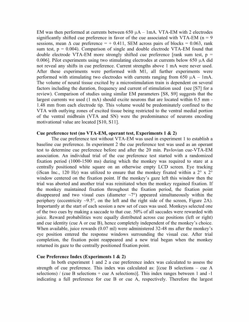
The cue preference test without VTA-EM was used in experiment 1 to establish a baseline cue preference. In experiment 2 the cue preference test was used as an operant test to determine cue preference before and after the 20 min. Pavlovian cue-VTA-EM association. An individual trial of the cue preference test started with a randomized fixation period (1000-1500 ms) during which the monkey was required to stare at a centrally positioned white square on an otherwise empty LCD screen. Eye tracking (iScan Inc., 120 Hz) was utilized to ensure that the monkey fixated within a 2° x 2° window centered on the fixation point. If the monkey’s gaze left this window then the trial was aborted and another trial was reinitiated when the monkey regained fixation. If the monkey maintained fixation throughout the fixation period, the fixation point disappeared and two visual cues (diameter ~7°) appeared simultaneously within the periphery (eccentricity ~9.5°, on the left and the right side of the screen, Figure 2A). Importantly at the start of each session a new set of cues was used. Monkeys selected one of the two cues by making a saccade to that cue. 50% of all saccades were rewarded with juice. Reward probabilities were equally distributed across cue positions (left or right) and cue identity (cue A or cue B), hence completely independent of the monkey’s choice. When available, juice rewards (0.07 ml) were administered 32-48 ms after the monkey’s eye position entered the response windows surrounding the visual cue. After trial completion, the fixation point reappeared and a new trial began when the monkey returned its gaze to the centrally positioned fixation point. Cue Preference Index (Experiments 1 & 2) In both experiment 1 and 2 a cue preference index was calculated to assess the strength of cue preference. This index was calculated as: [(cue B selections – cue A selections) / (cue B selections + cue A selections)]. This index ranges between 1 and -1 indicating a full preference for cue B or cue A, respectively. Therefore the largest

difference in the cue preference index between two different blocks would be 2, representing a shift from a full preference for one cue to a full preference to another cue. Cue-VTA-EM Operant Reinforcement Test (Experiment 1) The cue-VTA-EM operant reinforcement tests were performed in experiment 1 and were identical to the baseline cue preference test with the only difference being the addition of VTA-EM. Tests were deemed either cue A-VTA-EM or cue B-VTA-EM depending on whether selections of cue A or cue B, respectively, were followed by VTA-EM. The selection of the cue associated with VTA-EM (e.g. cue A during the cue A-VTA-EM block) was followed by VTA-EM during 50% of the trials independent of whether that trial was followed by juice administrations. During VTA-EM trials, VTA-EM occurred 32-48 ms after the monkey’s eye position entered the response window surrounding the visual cue associated with VTA-EM.
Balanced juice administration during cue preference tests (Experiment 1 & 2)
The probability of juice reinforcement for the selection of both visual cues was held at 50% for all cue preference tests, performed with and without VTA-EM. More specifically, within a cue preference test there were 4 possible trial types (see Figure 2A). A random sequence generator created sequences of 8 trials such that each trial type occurred twice every 8 trials resulting in both cues being associated with 50% juice reward probability. Nonetheless, differences in the frequency that selected visual cues were followed by juice could still occur. Therefore, we have compared the percent of trials each cue selection was actually reinforced with juice during experiments 1 & 2.
Following the same division of the data from experiment 1 used in Figures S1A (M1) & S1C (M3), the mean percent of cue A and cue B selections followed by juice reward was calculated per session for the early and late halves of each block (baseline, cue B-VTA-EM, and cue A-VTA-EM). We then performed sign rank tests comparing the percent of trials cue A and cue B were followed by juice for each half block across sessions. Both M1 (n = 4 sessions, p >= 0.2, uncorrected for multiple comparisons) and M3 (n = 16 sessions, p >= 0.25, uncorrected for multiple comparisons) did not display any significant difference in the percent of selections followed by juice between cue A and cue B.
For experiment 2 we utilized the division of data used in Figures S2A (M2) & S2C (M3) and calculated the mean percent of cue A and cue B selections followed by juice administration for each preference test block before and after cue B-VTA-EM . Sign rank tests were then performed to determine whether there was a difference in the percent of trials followed by juice administration between cue A and cue B selections. No significant differences were found for either of the pairs of preference blocks for both M2 (n = 6 pairs of blocks, p >= 0.19, uncorrected for multiple comparisons) and M3 (n = 28 pairs of blocks, p >= 0.77, uncorrected for multiple comparisons). The lack of any significant differences in the percent of trials that cue A and cue B selections were followed by juice administration during the cue preference tests performed in experiment 1 and 2, confirms that juice reinforcement was well matched between cues.

Kalman filter reinforcement learning model (Experiment 1) Kalman filter reinforcement learning models were constructed using a freely
available toolbox (www.cs.bris.ac.uk/home/rafal/rltoolbox/). This toolbox and the following methods are based directly on Daw et al., (2006). The Kalman filter reinforcement learning model is a generalization of temporal difference learning that also tracks uncertainty about action value. This model assumes the subject’s assessment of the diffusion of action value is determined by the following parameters: STD of score (
€
σo), STD of diffusion (
€
σd ), decaying rate of action values (
€
λ ), and the converging value of action values (
€
θ ). On a particular trial t, the prior distribution over the actual mean payoffs
€
µi,t , where i represents the ith action (e.g. cue A or cue B selection), are independent Gaussians
€
N(µi,tpre,σ i,t
2pre ) . If the subject then selects action ct and receives reward rt, the posterior mean is calculated as:
€
µct ,tpost = µct ,t
pre + ktδ t
€
with prediction error
€
δ t = rt − µct ,tpre and learning rate
€
kt =σ c,t2pre /(σ ct ,t
2pre +σ o2)
The posterior variance for the action selected is:
€
σct ,t2post = (1− kt )σct ,t
2pre The posterior mean and variance for the action not selected remain unchanged. Factoring in the diffusion process, the prior distributions on the following trial are
€
µi,t+1pre = λµ
i ,t
post + (1− λ)θ and
€
σi,t+12pre = λ2σi,t
2post +σd2
The recursive process is initialized with prior distribution
€
N(µi,0pre,σ i,0
2pre ) . Learning in this reinforcement learning model is driven by the same type of error-driven learning rule as temporal difference learning with the addition of a parameter that tracks uncertainty
€
σi,t2 .
€
σi,t2 is used to determine the trial specific learning rate
€
kt . In general, uncertainty to decreases for sampled actions and increases for actions not sampled. The choice rule used to determine the probability
€
Ρ of selecting action i on trial t as a function of the estimated reward was a softmax rule. The softmax rule is:
€
Ρi,t =exp(βµi,t
pre )βµ j,t
pre
j∑
with exploration parameter β. For each monkey, two separate learning models were generated. One model used juice administration as the reward input while the other model used VTA-EM. For each of these models, the parameters
€
δd ,
€
σo ,
€
λ ,
€
θ ,
€
µi,0pre ,
€
σi,0pre , and
€
β were taken to be free. These parameters were fit to the subjects’ choice data by maximizing the likelihood of the observed actions selected

€
Ρcs ,t ,tt∏
s∏
compounded over sessions s and trials t, where
€
cs,t denotes the action selected during session s on trial t, and the underlying value estimates
€
µi,tpre and uncertainties
€
σi,tpre were
computed using the sequence of cue selections and reward outcomes through trial t - 1. A combination of nonlinear optimization algorithms (Matlab optimization toolbox) was used to optimize the parameter fits, together with a search of different starting locations. We report the negative log likelihoods (NLLs) as a measurement of the fit of the model (smaller NLLs denote the model more closely fits the behavioral data). For each model, we fit the behavior of an individual subject across all sessions performed of experiment 1 using a single instance of the following parameters:
€
δd ,
€
σo ,
€
λ ,
€
θ ,
€
µi,0pre ,
€
σi,0pre
To capture some of the inter-session variability we fit the exploration parameter
€
β separately for each session. For each subject, the quality of the behavioral fit (NLL) and the parameter fits for both models (VTA-EM and juice) are reported in Table S1. The VTA-EM and juice models were compared using the Akaike information criterion (AIC), which provides a relative measure of the quality of the statistical model for the given data set. AIC = 2K – 2ln(L); where L is the likelihood function of a given model and k is the number of free parameters in that model. We report ΔAIC = AICjuice – AICVTA-EM as the lower AIC value denotes the model that better fits the data. It is general practice when comparing models using AIC for ΔAIC < 2 to be considered equivalent models. In addition, we report the AICweight; AICweight = exp(ΔAIC/2). The AICweight provides a relative measure of likelihood that the VTA-EM model provides a better fit for the data than the juice model. In addition, comparisons of VTA-EM and juice reinforcement models using the Bayesian information criterion yielded highly similar results.
Pavlovian Cue-VTA-EM Association (Experiment 2)
In experiment 2, Pavlovian cue-VTA-EM association blocks were performed in between 400 trial cue preference test blocks. These cue-VTA-EM association blocks lasted 20 minutes and required no cue-linked operant behavior from the monkey. Monkeys performed a passive fixation task to obtain juice rewards (800 – 1200 ms between 0.03 ml juice rewards) while every 3500 – 6000 ms one of the two visual cues was randomly presented. VTA-EM occurred 400 ms into the 500 ms long presentation of one of the cues. During this block the other cue was presented just as often as the VTA-EM coupled cue, yet the second cue was never associated with VTA-EM. The mean number of cue-‐VTA-‐EM association trials per 20 minute association block was 97.71. Timing of trials and blocks (Experiments 1 & 2)
During all cue preference tests (experiments 1 & 2), trials within a given block were performed without downtime between successive trials, with the subsequent trial beginning when the subject returned its gaze to the centrally positioned fixation point. Between successive blocks (i.e. between preference test blocks or between a preference test block and a Pavlovian association block) the program that controlled the experiment had to be reloaded. Therefore there were no trials between blocks but there was a downtime of < 1 minute.

VTA-EM fMRI experiment (Experiment 3) The design of experiment 3 was identical to the Pavlovian association block of experiment 2 with the caveat that no visual cues were displayed. Therefore, the monkey performed a passive fixation task for juice rewards (800 – 1200 ms between 0.03 ml juice rewards) while VTA-EM and no VTA-EM events were uncoupled from the juice events and occurred every 3900 – 6400 ms. Individual runs of experiment 3 lasted for 610 s (305 TR at 2s/TR). EM parameters were identical to experiments 1-2 (bipolar, 200 ms, 200 Hz) except lower currents were utilized (100-392 µA). General linear model (GLM) analysis (Experiment 3)
Images were first reconstructed then realigned using a non-rigid slice-by-slice registration algorithm [S6]. The resultant images were next 3D motion-corrected within session, smoothed (FWHM 1.5 mm), and non-rigidly coregistered (www.nitrc.org/projects/jip) [S13] to 112 RM-SL space [S14]. We then performed a voxel-based fixed-effect analysis with SPM 5, following previously described procedures to fit a general linear model [S1, S5, S15, S16]. High- and low-pass filtering was employed prior to fitting the GLM. To account for head movement related artifacts, six motion-realignment parameters were used as covariates of no interest. Anatomical region of interest (ROI) definition (Experiment 3)
Anatomical ROI analysis was performed on 68 regions with separate left and right hemisphere ROIs. One group of ROIs was constructed from ROIs used in previous studies [S17-S19] (AIP, DO, F1, F2, F3, F4, F5a, F5c, F5p, F6, F7, FEF, FST, GrF, LIPa, LIPi, LB1, LB2, LST, MIP, MSTd, MSTv, MT, Opt, PFG, PF, PG, STPm, UB1, UB2, V1d, V1v, V2d, V2v, V3A, V3d, V3v, V4d, V4v, V6A, V6, VIPp). The remaining ROIs were constructed in 112 RM-SL space using a co-registered atlas [S20] (Amygdala, Area 1/2, Area 3a/3b, Area 10, Area 11, Area 12, Area 13, Area 14, Area 23, Area 24, Area 25, Area 32, area 45A, area 45B, area 46v, Caudate, Gustatory, Hippocampus, Insula, NA, PrCO, Putamen, SII, TEO, TE, TPO). No ROIs were made for midbrain structures but the center of mass and volume of these activations and the approximate structures they colocalize with are reported in Table S2.

ROI analysis (Experiment 3) The volume of activations within an anatomical ROI (Table S2) was determined
from the overlap of the anatomical ROIs (see anatomical ROI definition above) and significantly activated voxels. Separate thresholds for significantly activated voxels were used in the group analyses (FDR corrected, p = 0.001, cluster size 10 voxels) and the individual subject (M1, M2 and M3) analyses (FDR corrected, p = 0.02). To better describe the VTA-EM induced activations within these ROIs, functional ROIs were constructed from the volume of activated voxels within the group analysis. Using these functional ROIs, the PSC was then calculated. For each functional ROI, the raw fMRI signal was extracted and averaged across all voxels. The raw signal was then high-pass filtered (256 s) and an independent baseline was determined for each data point by calculating the moving average of the fMRI signal in a window of +/- 50 data points (+/- 100 s) [S21]. VTA-EM and no VTA-EM trials were then aligned at timepoint zero and a peri-stimulus time histogram was computed for each fMRI run. The mean PSC and SEM PSC were taken from the timepoint 6s after VTA-EM and no VTA-EM event onsets. Density of juice administration temporally surrounding VTA-EM events (Experiment 3)
The timing of VTA-EM and no VTA-EM events (3900 - 6400 ms) and juice administration (800 – 1200 ms) events were temporally uncorrelated in Experiment 3. The experiment was designed such that juice events were matched between VTA-EM and no VTA-EM events. To test this, we calculated the mean frequency of juice administration events surrounding VTA-EM and no VTA-EM events within +/- 1 s time-window for each fMRI run. Sign rank tests comparing the mean frequency of juice administration between VTA-EM and no VTA-EM events in experiment 3 found no significant difference for M1 (n = 12 fMRI runs, p = 0.84), M2 (n = 5 fMRI runs, p = 0.22) and M3 (n = 18 fMRI runs, sign rank test, p = 0.88). Unexpected juice reward fMRI experiment.
This dataset, is a subset of a dataset previously reported in [S22] (their experiment 2). Importantly, every other run of the fMRI data used in [S22] were used in this analysis of unexpected juice reward activity so that power of VTA-EM (n = 35 runs) and unexpected juice fMRI datasets (40 runs; M4, 20 runs; M5, 20 runs) were more comparable. The design consisted of two equiprobable, randomized trial types (fixation, juice). The monkeys had to maintain fixation during a randomly jittered 3500 – 6000 ms waiting period. During unexpected juice reward trials, 400 ms after the waiting period ended 0.2 ml juice reward was administered. During a fixation trial, no visual stimulus was presented but fMRI data were sampled from an equivalent time point (400 ms after wait period).

Supplemental References 1. Vanduffel, W., Fize, D., Mandeville, J.B., Nelissen, K., Van Hecke, P., Rosen,
B.R., Tootell, R.B., and Orban, G.A. (2001). Visual motion processing investigated using contrast agent-enhanced fMRI in awake behaving monkeys. Neuron 32, 565-577.
2. Tani, N., Joly, O., Iwamuro, H., Uhrig, L., Wiggins, C.J., Poupon, C., Kolster, H., Vanduffel, W., Le Bihan, D., Palfi, S., et al. (2011). Direct visualization of non-human primate subcortical nuclei with contrast-enhanced high field MRI. Neuroimage 58, 60-68.
3. Bondar, I.V., Leopold, D.A., Richmond, B.J., Victor, J.D., and Logothetis, N.K. (2009). Long-term stability of visual pattern selective responses of monkey temporal lobe neurons. PLoS One 4, e8222.
4. Bichot, N.P., Heard, M.T., and Desimone, R. (2011). Stimulation of the nucleus accumbens as behavioral reward in awake behaving monkeys. J Neurosci Methods 199, 265-272.
5. Leite, F.P., Tsao, D., Vanduffel, W., Fize, D., Sasaki, Y., Wald, L.L., Dale, A.M., Kwong, K.K., Orban, G.A., Rosen, B.R., et al. (2002). Repeated fMRI using iron oxide contrast agent in awake, behaving macaques at 3 Tesla. Neuroimage 16, 283-294.
6. Kolster, H., Mandeville, J.B., Arsenault, J.T., Ekstrom, L.B., Wald, L.L., and Vanduffel, W. (2009). Visual field map clusters in macaque extrastriate visual cortex. J Neurosci 29, 7031-7039.
7. Tehovnik, E.J., Tolias, A.S., Sultan, F., Slocum, W.M., and Logothetis, N.K. (2006). Direct and indirect activation of cortical neurons by electrical microstimulation. J Neurophysiol 96, 512-521.
8. Murasugi, C.M., Salzman, C.D., and Newsome, W.T. (1993). Microstimulation in visual area MT: effects of varying pulse amplitude and frequency. The Journal of neuroscience : the official journal of the Society for Neuroscience 13, 1719-1729.
9. Tehovnik, E.J., Slocum, W.M., and Schiller, P.H. (2004). Microstimulation of V1 delays the execution of visually guided saccades. The European journal of neuroscience 20, 264-272.
10. Matsumoto, M., and Hikosaka, O. (2009). Two types of dopamine neuron distinctly convey positive and negative motivational signals. Nature 459, 837-841.
11. Matsumoto, M., and Takada, M. (2013). Distinct representations of cognitive and motivational signals in midbrain dopamine neurons. Neuron 79, 1011-1024.
12. Daw, N.D., O'Doherty, J.P., Dayan, P., Seymour, B., and Dolan, R.J. (2006). Cortical substrates for exploratory decisions in humans. Nature 441, 876-879.
13. Mandeville, J.B., Choi, J.K., Jarraya, B., Rosen, B.R., Jenkins, B.G., and Vanduffel, W. (2011). fMRI of cocaine self-administration in macaques reveals functional inhibition of basal ganglia. Neuropsychopharmacology 36, 1187-1198.
14. McLaren, D.G., Kosmatka, K.J., Oakes, T.R., Kroenke, C.D., Kohama, S.G., Matochik, J.A., Ingram, D.K., and Johnson, S.C. (2009). A population-average MRI-based atlas collection of the rhesus macaque. Neuroimage 45, 52-59.

15. Friston, K.J., Holmes, A.P., Poline, J.B., Grasby, P.J., Williams, S.C., Frackowiak, R.S., and Turner, R. (1995). Analysis of fMRI time-series revisited. Neuroimage 2, 45-53.
16. Vanduffel, W., Fize, D., Peuskens, H., Denys, K., Sunaert, S., Todd, J.T., and Orban, G.A. (2002). Extracting 3D from motion: differences in human and monkey intraparietal cortex. Science 298, 413-415.
17. Nelissen, K., Borra, E., Gerbella, M., Rozzi, S., Luppino, G., Vanduffel, W., Rizzolatti, G., and Orban, G.A. (2011). Action observation circuits in the macaque monkey cortex. The Journal of neuroscience : the official journal of the Society for Neuroscience 31, 3743-3756.
18. Nelissen, K., and Vanduffel, W. (2011). Grasping-related functional magnetic resonance imaging brain responses in the macaque monkey. The Journal of neuroscience : the official journal of the Society for Neuroscience 31, 8220-8229.
19. Belmalih, A., Borra, E., Contini, M., Gerbella, M., Rozzi, S., and Luppino, G. (2009). Multimodal architectonic subdivision of the rostral part (area F5) of the macaque ventral premotor cortex. The Journal of comparative neurology 512, 183-217.
20. Saleem, K.S., and Logothetis, N.K. (2006). Combined MRI and Histology Atlas of the Rhesus Monkey Brain., (Amsterdam: Academic Press).
21. Cui, X., Stetson, C., Montague, P.R., and Eagleman, D.M. (2009). Ready...go: Amplitude of the FMRI signal encodes expectation of cue arrival time. PLoS Biol 7, e1000167.
22. Arsenault, J.T., Nelissen, K., Jarraya, B., and Vanduffel, W. (2013). Dopaminergic reward signals selectively decrease fMRI activity in primate visual cortex. Neuron 77, 1174-1186.