Embed Size (px)
Citation preview
8/3/2019 Ronnie Jansson- The Membrane Vacuum State
http://slidepdf.com/reader/full/ronnie-jansson-the-membrane-vacuum-state 1/107
Master of science thesis in physics
The Membrane Vacuum State
Ronnie Jansson
Institute for Theoretical Physics
Chalmers University of Technologyand
Goteborg University
Fall 2003

8/3/2019 Ronnie Jansson- The Membrane Vacuum State
http://slidepdf.com/reader/full/ronnie-jansson-the-membrane-vacuum-state 2/107
8/3/2019 Ronnie Jansson- The Membrane Vacuum State
http://slidepdf.com/reader/full/ronnie-jansson-the-membrane-vacuum-state 3/107
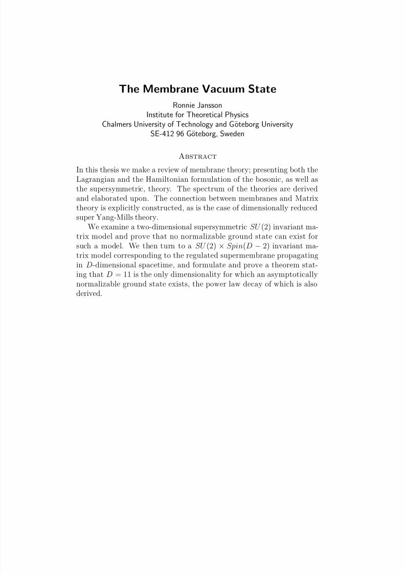
The Membrane Vacuum State
Ronnie JanssonInstitute for Theoretical Physics
Chalmers University of Technology and Goteborg UniversitySE-412 96 Goteborg, Sweden
Abstract
In this thesis we make a review of membrane theory; presenting both theLagrangian and the Hamiltonian formulation of the bosonic, as well asthe supersymmetric, theory. The spectrum of the theories are derived
and elaborated upon. The connection between membranes and Matrixtheory is explicitly constructed, as is the case of dimensionally reducedsuper Yang-Mills theory.
We examine a two-dimensional supersymmetric SU (2) invariant ma-trix model and prove that no normalizable ground state can exist forsuch a model. We then turn to a SU (2) × Spin(D − 2) invariant ma-trix model corresponding to the regulated supermembrane propagatingin D-dimensional spacetime, and formulate and prove a theorem stat-ing that D = 11 is the only dimensionality for which an asymptoticallynormalizable ground state exists, the power law decay of which is alsoderived.
8/3/2019 Ronnie Jansson- The Membrane Vacuum State
http://slidepdf.com/reader/full/ronnie-jansson-the-membrane-vacuum-state 4/107
Acknowledgments
My deepest thanks go to my supervisor Prof. Bengt E.W. Nilsson; for
welcoming me into the group, for choosing a very exciting topic for mythesis and for his willingness to answer all my questions along the way.
Next I would like to extend my thanks to the whole Elementary Par-ticle Theory/Mathematical Physics group for the very nice atmosphere.Special thanks goes to Viktor Bengtsson for his help in treating the dy-namics of the membrane and turning room O6106 into a tranquil havenof productivity.
Finally, my warmest thanks to my family and friends without whosecontributions this thesis would surely have been completed months ago.
Insane in the membraneInsane in the brain! - Cypress Hill, ”Insane in the brain”
iv
8/3/2019 Ronnie Jansson- The Membrane Vacuum State
http://slidepdf.com/reader/full/ronnie-jansson-the-membrane-vacuum-state 5/107
8/3/2019 Ronnie Jansson- The Membrane Vacuum State
http://slidepdf.com/reader/full/ronnie-jansson-the-membrane-vacuum-state 6/107
3.3.3 Duality . . . . . . . . . . . . . . . . . . . . . . . 42
3.3.4 M-theory . . . . . . . . . . . . . . . . . . . . . . 443.3.5 The BFSS conjecture . . . . . . . . . . . . . . . . 44
4 The Membrane Vacuum State 474.1 Overview and preliminaries . . . . . . . . . . . . . . . . 47
4.1.1 Current state of affairs . . . . . . . . . . . . . . . 474.1.2 A toy model ground state . . . . . . . . . . . . . 49
4.2 The SU (2) ground state theorem . . . . . . . . . . . . . 514.2.1 The model . . . . . . . . . . . . . . . . . . . . . . 524.2.2 The theorem . . . . . . . . . . . . . . . . . . . . . 58
4.3 The Proof . . . . . . . . . . . . . . . . . . . . . . . . . . 60
4.3.1 The d = 2 case . . . . . . . . . . . . . . . . . . . 604.3.2 Power series expansion of Qβ . . . . . . . . . . . 614.3.3 The equation at n = 0 . . . . . . . . . . . . . . . 644.3.4 Extracting allowed states . . . . . . . . . . . . . . 67
4.4 A numerical method . . . . . . . . . . . . . . . . . . . . 69
5 Conclusions 73
A Notation and Conventions 77A.1 General conventions . . . . . . . . . . . . . . . . . . . . . 77A.2 List of quantities . . . . . . . . . . . . . . . . . . . . . . 79
B Proof of κ-symmetry 85B.1 Preliminaries . . . . . . . . . . . . . . . . . . . . . . . . 85B.2 The proof . . . . . . . . . . . . . . . . . . . . . . . . . . 86
C Some explicit calculations in the d = 3 case 93
Bibliography 97
vi
8/3/2019 Ronnie Jansson- The Membrane Vacuum State
http://slidepdf.com/reader/full/ronnie-jansson-the-membrane-vacuum-state 7/107
1
Introduction
Membrane theory has a rather peculiar history and can trace its originsback to the very depths of the sixties, thus predating the emergence of its more illustrious and celebrated sibling, string theory. The birthplaceof membrane theory, like many other grand ideas, was in the brilliantmind of Dirac [1]. In 1962, Dirac was pursuing an alternative model forthe electron and put forth the hypothesis that it should correspond to avibrating membrane. The resultant theory was plagued with many dif-
ficulties, however, and was soon abandoned to posterity. Some interestwas later rekindled in the 1970’s; along with the birth of string theorythe strict adherence to a paradigm of a four-dimensional world containingzero-dimensional objects was seriously questioned (Dirac had been aheadof his time) and having thus in strings gone from zero to one dimension,the next step was conceptually easy. During this time the quantum me-chanics of the membrane was analyzed, and the membrane itself was nowutilized in various models for hadrons. Still plagued by many problemsmembrane theory was left in the cradle while string theory grew up fastand hit puberty, and eventually was elevated to the exalted rank of acandidate to the Theory of Everything. When the first ”superstring rev-olution” hit the physics departments in 1984 and propelled string theoryinto respectable mainstream physics the membrane spectrum had beenfound continuous in the classical theory but discrete in the quantum case.This rare property of the Hamiltonian was investigated in [2] and is avery fortuitous trait as a continuous spectrum would spell disaster for afirst quantized theory.
So far everything have concerned only the bosonic membrane, butif its aspirations are to describe Nature membrane theory must addfermions into the mix. The huge success in incorporating fermions with
1
8/3/2019 Ronnie Jansson- The Membrane Vacuum State
http://slidepdf.com/reader/full/ronnie-jansson-the-membrane-vacuum-state 8/107
2 Chapter 1 Introduction
bosons in string theory via supersymmetry hinges on a crucial property
called κ-symmetry. At first believed exclusive to strings, κ-symmetrywas eventually generalized to membranes by Hughes, Liu and Polchin-ski [3] in 1986. As the newly christened supermembrane burst upon thescene a flurry of papers was published regarding the emergent theory.One important contribution was the realization that the type IIA super-string in ten dimensions could be obtained from the supermembrane ineleven dimensions by wrapping up one of the membrane’s dimensions ona circle [4]. Another aspect which later turned out to be very intriguingand which plays a vital part in this thesis is the possibility to regularizethe supermembrane [5] in terms of certain supersymmetric matrix mod-els belonging to some finite group, e.g., SU (N ). The supermembrane isthen recovered in the N → ∞ limit. These matrix models were stud-ied [6] some years prior to the discovery of this connection, and then inthe context of dimensionally reduced supersymmetric Yang-Mills theory.
A problem now looming over the membrane community was the ev-idence pointing to a continuous spectrum for the quantum supermem-brane. Until this was a proven fact, however, research continued unper-turbed. The verdict came in a paper in 1989 [7], and the supermembranewas found guilty of continuity and subsequently condemned to the prisonof bad ideas. Membrane theory thus lay dormant for some years until thesecond superstring revolution arrived in 1995 and revitalized the entire
community. It now became apparent that the ten dimensions inherentin string theory was not enough to describe Nature. Furthermore, thefive different string theories were unified and could trace themselves toa (M)other theory living in eleven dimensions, the very same dimension-ality where the supermembrane assume its most appealing form. Stringtheory was superseded by the newly baptized ”M-theory” as the numberone candidate for the final theory. Little was known about this mysteri-ous theory other than that it had eleven-dimensional supergravity as alow-energy limit and that it tied together the various string theories withdifferent dualities.
Many drastic breakthroughs were also made directly related to mem-branes. Townsend kick-started 1996 with a paper [8] suggesting that thecontinuous spectrum was not a failure of first quantization but insteadimplied a second quantized theory from the very beginning, thus turningthe greatest weakness of the theory into a virtue. Slightly prior to this,Witten showed [9] a connection between D0-branes and matrix theoryand thus tying them together with supermembranes. Based on this workBanks, Fischler, Shenker and Susskind made a bold conjecture claimingthat these super matrix models in the large N limit exactly describedM-theory in the infinite momentum frame. As these matrix models were
8/3/2019 Ronnie Jansson- The Membrane Vacuum State
http://slidepdf.com/reader/full/ronnie-jansson-the-membrane-vacuum-state 9/107
1.1 Outline of this thesis 3
inexorably linked to supermembranes interest exploded in matrix theory
as well as membrane theory.As membranes now became the focus of much research the old ques-
tion of the existence and feasibility of obtaining its ground state aroseagain, this time with somewhat increased urgency as the stakes, andconsequently the rewards, were considerably higher. Furthermore, ma-trix theory offered a new set of tools in attacking the problem. It turnedout that the avenue of choice in confronting the membrane vacuum stateis by trying to find the vacuum state of the corresponding SU (N ) matrixmodel. From 1997 and onwards work on this subject has been conductedwith varying degrees of success. A large contribution to this field is due
to the incessant efforts of Jens Hoppe and collaborators who have madepromising advances mainly in the SU (2) case, which is something wewill study in detail in this thesis. While N = 2 is only a modest part of N → ∞, its positive answer to the existence of a normalizable groundstate can hopefully be generalized to arbitrary N .
We conclude this brief exposition of the history of membrane theoryby stressing the fact that despite its bumpy ride between pre-eminenceand obscurity membranes are now firmly established as an intricate partof M-theory. In light of this importance it is no surprise that our lack of an explicit membrane vacuum state or even proof that such a state existis frustrating and simultaneously an incentive to continue the search for
that state.
1.1 Outline of this thesis
This thesis is to a large part a review of membrane theory, although itscontent is strongly tilted towards tools needed to analyze the superme-mbrane vacuum state from the vantage point of matrix theory.
We begin the thesis with a treatment of the basic properties of themembrane. Before confronting the full-fledged supermembrane we care-
fully work through the less intimidating bosonic membrane, acquiringmuch needed tools and formalism along the way. Specifically, we willanalyze the membrane in both Lagrangian and Hamiltonian formalism,discuss ways of quantization and take the membrane to the lightconegauge, and discover an important residual symmetry, area preservingdiffeomorphisms. We then continue with a very condensed introduc-tion of supersymmetry, giving only the basics needed and swiftly movingon to discussing the viable choices of implementing supersymmetry intomembrane theory. The stage is thus set for the entrance of the superme-mbrane, but instead we analyze what restrictions supersymmetry place
8/3/2019 Ronnie Jansson- The Membrane Vacuum State
http://slidepdf.com/reader/full/ronnie-jansson-the-membrane-vacuum-state 10/107
4 Chapter 1 Introduction
on our theory. Strings and membranes are but two cases of the more
general p-branes, extended objects of p dimensions. As we will show inthe section entitled ”the brane scan” supersymmetry gives us a very def-inite answer as to which values of p are allowed and in what dimensionsof spacetime they can live in. Having done this we examine the actionof the super p-brane and its attendant symmetries, an easy feat when wehave the bosonic case still fresh in our minds.
The next chapter continues the treatment of supermembranes. Westart with the Hamiltonian perspective and note the conceptually im-portant area preserving diffeomorphisms (APD) and its implications onthe dynamics of the membrane. The APD algebra is investigated further
as we start building the bridge between supermembranes and matrixtheory. We thus perform the regularization of the membrane. In thefollowing section we treat another route to matrix theory, namely thedimensional reduction of super Yang-Mills theory. We then move onto analyze the spectrum of both the bosonic and supersymmetric mem-brane, in the bosonic case giving a full proof of the continuous spectrumfor the classical theory and the discrete nature of the quantum case. Forthe supermembrane we illustrate the continuous spectrum by using a toymodel.
The remaining part of chapter 3 takes on a slightly different flavor aswe present a brief overview of what has become known as M-theory. The
objective is in part to see the supermembrane in its natural surroundingsand in part to give the author the opportunity to examine issues not di-rectly connected with the subject matter of this thesis. Briefly, we touchupon subjects like supergravity, strings and duality. A slightly more in-depth discussion of the very important BFSS conjecture concludes thechapter.
The last chapter carries the same title as the thesis and is where wego into greater detail, narrowing our scope to the conjectured membranevacuum state. After a short chronological overview of the research thathas been done on the subject, a toy model ground state is investigated
using a method similar to the one used in the subsequent theorem re-garding the ground state of the SU (2) invariant matrix model. We thenpresent in detail the model and method used for analyzing this groundstate, formulate the theorem [10] and examine the proof. The chapteris concluded by some remarks regarding a novel computational methodthat recently have been applied to similar problems.
In the three appendices we go through the notation and conventionsused in the thesis, perform the proof of the κ-symmetry of the superme-mbrane, and finally present some calculations related to the main groundstate theorem.
8/3/2019 Ronnie Jansson- The Membrane Vacuum State
http://slidepdf.com/reader/full/ronnie-jansson-the-membrane-vacuum-state 11/107
1.2 A remark 5
1.2 A remark
While I hold no illusion as to whether this thesis will ever be read beyondthe acknowledgments, or perhaps this introduction, by anyone except mysupervisor (who gets paid to do it), I feel compelled to be at least some-what considerate of the readability of the text. Most scientific texts areby their very nature dull and austere, and this thesis is no exception.However, austerity can be a positive characteristic as it focuses on theonly things of importance, without sugar-coating it. Moderation is asusual the key, as some authors take this scheme too far and condensetheir material into beautifully aesthetic pieces of writing, completely un-readable to a novice of the field.
While on the subject of aesthetics I would like to comment on chapter 4and its complete lack of aesthetic expressions. Though some are justunattractive, the vast majority are plain hideous. The reasons for this ismy strict adherence to keeping the notation of the original papers, whichin this case spawned said obscenities. My only justification would be toremark that in an attempt to make the expressions more pleasing to theeye the clarity of the exposition might be lost; an unfair trade to be sure.
Despite the above, I have imagined a collection of enthusiastic andattentive readers and done my best to present the material in as a peda-gogical way as possible, striving to heed the words of a man much wiser
that myself: ”Beware the lollipop of mediocrity. Lick once and you suckforever.”

8/3/2019 Ronnie Jansson- The Membrane Vacuum State
http://slidepdf.com/reader/full/ronnie-jansson-the-membrane-vacuum-state 12/107
6 Chapter 1 Introduction
8/3/2019 Ronnie Jansson- The Membrane Vacuum State
http://slidepdf.com/reader/full/ronnie-jansson-the-membrane-vacuum-state 13/107
2
The SupermembraneIn this initial chapter we review the basic properties of the supermem-brane. Emphasis is put on aspects relevant to the search for a membranevacuum state. Although the majority of the material in this chapterapplies to extended objects of higher (and lower) dimension than two,the 2-brane, or membrane, is ultimately the most interesting case for thepurpose of this thesis and thus the one we will treat more thoroughly.The first part of this chapter concerns the bosonic theory and deals with
membranes exclusively, while the later part of the chapter incorporatessupersymmetry and treat the more general case of p-branes.More in-depth treatments of the supermembrane abound; good ones
include [11, 12,13].
2.1 The bosonic membrane
In this section an introduction to the bosonic membrane is made. Anunderstanding of bosonic membranes will be of great help when we wantto treat the more involved supermembrane.
2.1.1 The membrane action
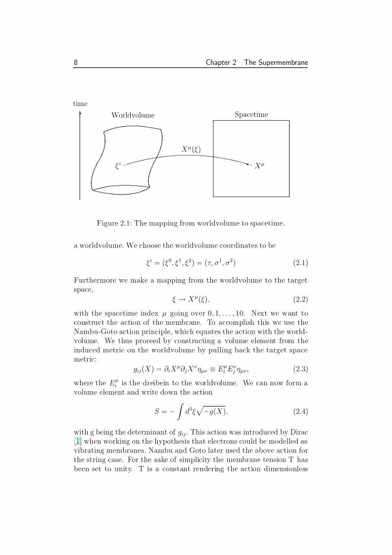
In the most general case we have a p-dimensional extended object, a p-brane, propagating in a curved target space of D dimensions. We will,however, restrict ourselves to the 2-brane in 11-dimensional spacetime.The reason for this will become clear when we discuss the supermem-brane. For simplicity we also choose spacetime to be flat with Minkowskimetric ηµν . In analogy with a particle or string sweeping out a worldlineor worldsheet respectively, the time evolution of a membrane will create
7
8/3/2019 Ronnie Jansson- The Membrane Vacuum State
http://slidepdf.com/reader/full/ronnie-jansson-the-membrane-vacuum-state 14/107
8 Chapter 2 The Supermembrane
Worldvolume
X µ(ξ)
Spacetime
ξi X µ· ·z
T
time
Figure 2.1: The mapping from worldvolume to spacetime.
a worldvolume. We choose the worldvolume coordinates to be
ξi = (ξ0, ξ1, ξ2) = (τ, σ1, σ2) (2.1)
Furthermore we make a mapping from the worldvolume to the target
space,ξ → X µ(ξ), (2.2)
with the spacetime index µ going over 0, 1, . . . , 10. Next we want toconstruct the action of the membrane. To accomplish this we use theNambu-Goto action principle, which equates the action with the world-volume. We thus proceed by constructing a volume element from theinduced metric on the worldvolume by pulling back the target spacemetric:
gij(X ) = ∂ iX µ∂ jX ν ηµν ≡ E µi E ν j ηµν , (2.3)
where the E µi is the dreibein to the worldvolume. We can now form avolume element and write down the action
S = −
d3ξ
−g(X ), (2.4)
with g being the determinant of gij . This action was introduced by Dirac[1] when working on the hypothesis that electrons could be modelled asvibrating membranes. Nambu and Goto later used the above action forthe string case. For the sake of simplicity the membrane tension T hasbeen set to unity. T is a constant rendering the action dimensionless
8/3/2019 Ronnie Jansson- The Membrane Vacuum State
http://slidepdf.com/reader/full/ronnie-jansson-the-membrane-vacuum-state 15/107
2.1 The bosonic membrane 9
and can be brought back by simple dimensional analysis. A classically
equivalent action,
S = −
d3ξ√−ggij E µi E jν +
1
2
√−g, (2.5)
was introduced by Howe and Tucker, and is commonly known as thePolyakov action. In this action gij is treated as an auxiliary field. How-ever, if we vary the action with respect to gij we find that gij is just theinduced metric. Substituting this into the Polyakov action we recover theNambu-Goto action, thus the classical equivalence. As expected then,varying either action with respect to X µ yields the same equations of
motion,∂ i(
√−ggij E µ j ) = 0. (2.6)
The bosonic membrane exhibit a global symmetry determined by thetarget space geometry. In the case of D = 11 Minkowski space it issimply an invariance under eleven dimensional Poincare transformations
δX µ = aµ + ωµν X ν . (2.7)
Local symmetry comes in the guise of worldvolume reparametrizationinvariance
ξi
→ξi(ξ0, ξ1, ξ2). (2.8)
2.1.2 The Hamiltonian formulation
To leave the lagrangian formalism in favor of the hamiltonian variety wemake use of Dirac’s method for constrained hamiltonian systems [14].We begin by forming the conjugate momenta
P µ =δL
δ(∂ 0X µ), (2.9)
where the lagrangian is of the Nambu-Goto type. If we introduce thefollowing shorthand notation
X µ =∂X µ
∂τ X µ =
∂X µ
∂σ1X µ =
∂X µ
∂σ2, (2.10)
the conjugate momenta takes the form
P µ = L−1
X µ((X X )2 − X 2X 2) + X µ((XX )X 2
− (X X )(X X ))X µ((X X )X 2 − (XX )(X X ))
. (2.11)
8/3/2019 Ronnie Jansson- The Membrane Vacuum State
http://slidepdf.com/reader/full/ronnie-jansson-the-membrane-vacuum-state 16/107
10 Chapter 2 The Supermembrane
From the above we can then obtain a set of primary constraints for the
membrane,
φ1 ≡ P · X ≈ 0 (2.12)
φ2 ≡ P · X ≈ 0 (2.13)
φ3 ≡ P 2 − (X X )2X 2X 2 ≈ 0, (2.14)
where ≈ 0 means ”weakly zero”, i.e., the constraints may have nonzeroPoisson (or Dirac) brackets with the phase-space variables.
Without any primary constraints the Hamiltonian would simply begiven by
H 0 = dσ1dσ2(X µP µ− L
). (2.15)
As primary constraints are present, however, we can add arbitrary linearcombinations of the constraints to H 0 without effecting the dynamicsof the membrane. Furthermore, as H 0 is easily found to be zero theHamiltonian is just constructed from the primary constraints alone,
H =
dσ1dσ2
λ(τ, σ1, σ2)φ1 + µ(τ, σ1, σ2)φ2 + ν (τ, σ1, σ2)φ3
,
(2.16)with λ,µ,ν arbitrary functions. These functions in turn are set when wedecide on a particular gauge. To move on to the equation of motion we
first need to introduce the functional Poisson bracket,
g, H =
dσ1dσ2
δg
δX (τ, σ1, σ2)· δH
δP (τ, σ1, σ2)
− δg
δP (τ, σ1, σ2)· δH
δX (τ, σ1, σ2)
. (2.17)
Hamilton’s equation of motion for a general dynamical functional of theform g[P µ, X µ, τ ] is then
g =dg
dt= g, H +
∂g
∂t. (2.18)
Now it is important to note that the above constraints can be used afterthe bracket operation has been performed, thus forcing λ,µ,ν to act asconstants in the Poisson brackets. To see that the primary constraintsare time-independent we must show that
φi = φi, H (2.19)
holds true on the subspace of the phase space where (2.12)-(2.14) arevalid. In our case, where H 0 is identically zero, we only have to showthat
φi, φ j = C ijk φk, (2.20)
8/3/2019 Ronnie Jansson- The Membrane Vacuum State
http://slidepdf.com/reader/full/ronnie-jansson-the-membrane-vacuum-state 17/107
2.1 The bosonic membrane 11
where C ijk are arbitrary functions of X µ and P µ. Calculating C ijk , while
not especially complicated, are painfully time-consuming and hence leftas an exercise to the reader. In any case, a calculation will show that C ijk
are indeed functions of X µ and P µ only [15], i.e. the primary constraintsare conserved. The dynamics of the membrane is then fully specified bythe constraints (2.12)-(2.14) and the equation of motion (2.18) togetherwith the full Hamiltonian
H =
dσ1dσ2
λ(X · P ) + µ(X · P ) + ν (P 2 − (X · X )2 + X 2X 2)
.
(2.21)The next logical step in our treatment of the membrane would be to
proceed to a quantum theory. We are then presented with two choices.We can use covariant quantization to turn X µ and P µ into operatorssatisfying the canonical commutation relations and turn the constraintsalong with the Hamiltonian into operator expressions. The other choice,which we will treat later, entails reducing the degrees of freedom intoan independent set of variables and then quantizing these variables. Avirtue of the latter method is the lack of constraints in the quantumtheory, while the downside is the loss of explicit covariance.
2.1.3 Covariant quantization
We begin by replacing the canonical variables with operators
X µ → X µ, P µ → P µ. (2.22)
These operators are then required to satisfy the canonical commutationrelations:
[X µ(τ, σ1, σ2), P ν (τ, σ1, σ2)] = 4π2igµν δ(σ1 − σ1)δ(σ2 − σ2) (2.23)
[X µ(τ, σ1, σ2), X ν (τ, σ1, σ2)] = 0 (2.24)
[P µ(τ, σ1, σ2), P ν (τ, σ1, σ2)] = 0. (2.25)
To derive (2.23) and also to get rid of ordering ambiguities we have
assumed H, X µ
and P µ
to be Hermitian. To proceed from (2.21) wemake a gauge choice which will make the equation of motion for X µ
become a linear second order differential equation. To accomplish thiswe set the multipliers to
λ = 0, µ = 0, ν =1
2. (2.26)
We now get the quantum Hamiltonian
H =1
2
dσ1dσ2
P 2 − (X 2X 2 + X · X )2
, (2.27)
8/3/2019 Ronnie Jansson- The Membrane Vacuum State
http://slidepdf.com/reader/full/ronnie-jansson-the-membrane-vacuum-state 18/107
12 Chapter 2 The Supermembrane
and the constraints (2.12)-(2.14) in operator form:
φ1 = X · P + P · X (2.28)
φ2 = X · P + P · X (2.29)
φ3 = P 2 − X 2X 2 + (X · X )2. (2.30)
These, in turn, are implemented by requiring
φi |P = 0, (2.31)
for all physical states |P (in the Heisenberg picture). However, actuallyputting the covariant quantization to some use is difficult. As in string
theory ghosts would likely appear. In the string case the removal of theghosts are made easy by the possibility to express the Hamiltonian interms of creation and annihilation operators. The lack of creation andannihilation operators in the membrane case, however, would make saidghosts very troublesome to exorcise. We therefore drop the discussion of covariant quantization without further ado.
2.1.4 The lightcone gauge
To learn more about the membrane we need to choose a particular gaugein which to analyze the inherent physics of the membrane. As in string
theory, the so-called lightcone gauge proves to be advantageous. To enterthe lightcone gauge we first introduce the lightcone coordinates
X ± =1√
2(X 10 ± X 0) (2.32)
and denote the transverse coordinates by
X (ξ) = X a(ξ), a = 1, . . . , 9 (2.33)
thus reducing the number of coordinates from 11 to 9. We then makethe gauge choice
X +(ξ) = X +(0) + τ, (2.34)
hence implying∂ iX + = δi0. (2.35)
We can now write down the induced metric in the lightcone gauge:
grs = ∂ r X · ∂ s X ≡ grs,
g0r = ∂ rX − + X · ∂ r X ≡ ur,
g00 = 2X − + X 2.
8/3/2019 Ronnie Jansson- The Membrane Vacuum State
http://slidepdf.com/reader/full/ronnie-jansson-the-membrane-vacuum-state 19/107
2.1 The bosonic membrane 13
The determinant becomes
g = −∆g, (2.36)
where
g ≡ detgrs, grsgst = δrt , ∆ = −g00 + urgrsus. (2.37)
By virtue of the above, the Lagrangian takes the simple form
L = −
g∆. (2.38)
The Hamiltonian formulation is, however, of greater interest to us. We
thus form the canonical momenta P and P + conjugate to X and X −,respectively:
P =∂ L∂ X
=
g
∆
X − urgrs∂ s X
, (2.39)
P + =∂ L
∂ X −=
g
∆. (2.40)
The Hamiltonian density is
H = P ·
X + P
+ ˙X −
− L =
P 2 + g
2P + . (2.41)
With the primary constraint
φr = P · ∂ r X + P +∂ rX − ≈ 0 (2.42)
and Lagrange multiplier cr we construct the total Hamiltonian [14]
H total =
d2σH + crφr, (2.43)
which has no secondary constraints. The gauge condition (2.34) has a
residual invariance under the spatial diffeomorphism
σr → σr + ξr(τ, σ), (2.44)
which will transform ur as follows:
ur → ur − ∂ 0ξr + ∂ sξrus − ξs∂ sur. (2.45)
This will allow us to impose the gauge condition
ur = 0, (2.46)
8/3/2019 Ronnie Jansson- The Membrane Vacuum State
http://slidepdf.com/reader/full/ronnie-jansson-the-membrane-vacuum-state 20/107
14 Chapter 2 The Supermembrane
since ”∂ 0ξr” is independent of ur and can be chosen to cancel the other
terms. From this it follows that the Hamilton equations correspondingto H total imply that cr = 0 and moreover that
∂ 0P + = 0. (2.47)
As P +(σ) transforms as a density under diffeomorphisms we can rewriteit as a constant times a density, i.e.,
P +(σ) = P +0
w(σ), (2.48)
where we will normalize the function
w(σ) according to
d2σ
w(σ) = 1. (2.49)
The function wrs(σ) can be interpreted as a 2-by-2 spatial metric on themembrane itself, and w(σ) as the metric determinant. Except for beingnon-singular the metric is arbitrary. However, it is important to notethat no physical quantity can be allowed to depend on our choice of met-ric. This independence is a consequence of the invariance of the theoryunder area preserving diffeomorphisms, together with the fact that, ex-cept for the Lorentz boost generators, the metric wrs(σ) only appears invarious physical quantities in the guise of the metric determinant w(σ).
Furthermore, area preserving diffeomorphisms, which will be treated inthe next section, leave by definition
w(σ) invariant. From the above
expressions we see that P +0 is the membrane momentum in the X − di-rection, and
P +0 =
d2σP +. (2.50)
The center of mass momenta is given by
P 0 ≡
d2σ P (σ), (2.51)
P −0 ≡ d2σH, (2.52)
whereby the mass formula for the membrane becomes
M2 = −2P +0 P −0 − P 20 =
d2σ
[ P 2] + g
w(σ)
. (2.53)
The relation between the Hamiltonian and mass being
H = M2 = T + V. (2.54)
8/3/2019 Ronnie Jansson- The Membrane Vacuum State
http://slidepdf.com/reader/full/ronnie-jansson-the-membrane-vacuum-state 21/107
2.1 The bosonic membrane 15
The meaning of the prime in equation (2.53) is the exclusion of the zero
mode, X 0, defined by
X 0 ≡
d2σ
w(σ) X (σ). (2.55)
The center of mass kinematics are determined by the theory of a free rela-tivistic particle, while the membrane dynamics are governed by equation(2.53). An obvious observation regarding the mass formula is the lackof explicit dependence on the coordinate X −. This coordinate is insteaddetermined by the gauge condition ur = 0, i.e.,
∂ rX − =−
X ·
∂ r X. (2.56)
For X − to be a globally defined function of σr (∂ 0 X · ∂ r X ) = 0 (2.57)
must be fulfilled for any closed curve on the membrane. This locallyamounts to the condition
φ = rs(∂ r P · ∂ s X ) ≈ 0. (2.58)
2.1.5 Area preserving diffeomorphisms
The gauge condition (2.58) used in the previous section leave a residualgauge symmetry of the lightcone Hamiltonian. This reparametrizationinvariance answers to the name of APD, area preserving diffeomorphisms.
Let us introduce a bracket operation on any two functions A(σ) andB(σ) in the shape of
A, B(σ) ≡ rs w(σ)
∂ rA(σ)∂ sB(σ), (2.59)
which is manifestly antisymmetric,
A, B = −B, A, (2.60)
and satisfies the Jacobi identity
A, B, C + C, A, B + B, C, A = 0. (2.61)
The bracket is thus a Lie bracket and together with the functions on themembrane forms an infinite dimensional Lie algebra. We can now rewritethe potential density g as
g = X a, X b2, (2.62)
8/3/2019 Ronnie Jansson- The Membrane Vacuum State
http://slidepdf.com/reader/full/ronnie-jansson-the-membrane-vacuum-state 22/107
16 Chapter 2 The Supermembrane
which turn the Hamiltonian (2.53) into
M2 =1
2
d2σ
[ P 2(σ)]
w(σ)+
w(σ)X a, X b2
. (2.63)
From this expression we can deduce that X a, X b2 is a measure of thepotential energy of the membrane. From the fact that
X a, X b =rs w(σ)
∂ rX a∂ sX b (2.64)
is just the area element of the membrane pulled back into spacetime weconclude that a membrane can change its shape and form, as long as
the area remains constant, without any change in its potential energy.This is of course the meaning of area preserving diffeomorphisms andcorrespond to the transformation
σr → σr + ξr(σ) (2.65)
with∂ r(
w(σ)ξr(σ)) = 0. (2.66)
Locally, this amounts to
ξr(σ) =rs
w(σ)∂ sξ(σ). (2.67)
It is also worth noting that the variation of a function f under an in-finitesimal area preserving reparametrization is
δf = −ξr∂ rf = ξ, f . (2.68)
Furthermore we can rewrite the constraint (2.58) in the form
φ(σ) ≡ P , X (2.69)
and verify that the mass M actually commutes with this constraint.
2.2 SupersymmetryThe field of supersymmetry has since its birth in the early 1970s grown tobecome one of the most expansive and fundamental theories within thedomain of theoretical physics. It would be hubris to attempt to pen downa self-contained review of such an encompassing field, so excluding somebrief introductory words this section will only present facts pertinent tomembranes. Numerous good reviews of supersymmetry exists; if unableto get ones hands on the elusive [16] the more readily available [17] and[18] will suffice.
8/3/2019 Ronnie Jansson- The Membrane Vacuum State
http://slidepdf.com/reader/full/ronnie-jansson-the-membrane-vacuum-state 23/107
2.2 Supersymmetry 17
2.2.1 Basics
Supersymmetry is a proposed symmetry linking fermions and bosonstogether. In essence, every spin-12 particle would have a spin-1 siblingand vice versa. The properties of these twin particles would be the sameas the original ones except for the spin and the name which, incidentally,is always more funny sounding for the supersymmetric twin (slepton,wino, higgsino etc.).
The only symmetries possible for the S-matrix (and hence also theLagrangian) in particle physics was shown in a classical paper in 1967 byColeman and Mandula [19] to be:
• Spacetime symmetries, Poincare invariance, i.e., the semi-directproduct of translations and Lorentz rotations.
• Internal global symmetries, related to conservation of quantumnumbers like electric charge and isospin.
• Discrete symmetries, C(harge), P(arity) and T(ime).
In deriving the Coleman-Mandula theorem one of the assumptions madeis that the S-matrix involves only commutators. By relaxing this con-straint and allowing for anticommutating generators as well, room ismade for supersymmetry; an extension of the spacetime symmetry men-tioned above (resulting in a super-Poincare algebra). Later, in 1975, itwas proved [20] that supersymmetry is the only additional symmetryallowed under the aforementioned assumptions.
The operator Q that realizes supersymmetry is thus an anticommu-tating spinor, with
Q |Boson = |Fermion and Q |Fermion = |Boson . (2.70)
Q and its hermitian conjugate Q† is then by the extension of the Coleman-Mandula theorem forced to satisfy the algebra
Q, Q† = P µ (2.71)
Q, Q = Q†, Q† = 0 (2.72)
[P µ, Q] = [P µ, Q†] = 0, (2.73)
where we have suppressed the spinor indices on Q and Q†, and where P µ
is the generator of translations.Irreducible representations of the supersymmetry algebra called su-
permultiplets contain both bosonic and fermionic states (superpartners of each other). If |Ω and |Ω belong to the same supermultiplet, then |Ω
8/3/2019 Ronnie Jansson- The Membrane Vacuum State
http://slidepdf.com/reader/full/ronnie-jansson-the-membrane-vacuum-state 24/107
18 Chapter 2 The Supermembrane
is by definition proportional to some combination of Q and Q† acting on
the superpartner state |Ω (up to spacetime translations and rotations).Now, since the (mass)2 operator, −P 2, commutes with Q, Q† and allspacetime translation and rotation operators the particles contained inthe same supermultiplet must necessarily have identical eigenvalues of −P 2 and hence equal mass. In addition to this, the operators Q andQ† commute with the generators of gauge transformations. This impliesthe fact that superpartners share the same properties of color degrees of freedom, electric charge and weak isospin.
To make the transition from bosonic membranes to supermembraneswe have to introduce supersymmetry. We are then presented with twoobvious choices; either we introduce supersymmetry locally on the mem-brane worldvolume (producing a so-called spinning membrane) or on thetarget space (yielding superspace). A third option would be to simulta-neously make use of both these approaches, resulting in something calledsuperembeddings [21]. This last option, though perhaps the most desir-able, is plagued with many difficulties and while research in this field isstill being conducted we will not touch on the subject any further.
2.2.2 Worldvolume supersymmetry
Introducing supersymmetry on the worldvolume of a p-brane would pro-
duce (p+1)-dimensional ”matter” supermultiplets (X µ, χµ), with µ =0, 1, . . . , D and χ a worldvolume spinor. In the string case, p = 1, thisyields the spinning string of Ramond, and Neveu and Schwarz. Aftersome GSO projections the obtained spectrum is exactly that of a space-time supersymmetric theory. Furthermore, the resulting action is equiv-alent to the normal Green-Schwarz superstring action. An attempt toconstruct a spinning membrane was made in [22]. However, the aboveprocedure led to the inclusion of an Einstein-Hilbert term,
√−gR, whentrying to supersymmetrize the cosmological term
√−g in the bosonicaction. These problems later grew into a no-go theorem for spinning
membranes [23].
2.2.3 Superspace
The obvious alternative to the spinning membrane is to introduce su-persymmetry on the background space. This is accomplished simply byadding a number of anticommutating fermionic coordinates, θα(ξ), to thebosonic ones, X µ(ξ). Thus yielding the superspace coordinates
Z M = (X µ, θα). (2.74)
8/3/2019 Ronnie Jansson- The Membrane Vacuum State
http://slidepdf.com/reader/full/ronnie-jansson-the-membrane-vacuum-state 25/107
2.3 Super p-branes 19
The fermionic coordinates, however, do not represent any position in
spacetime per se, and is better viewed as ”directions”.
2.2.4 Experimental verification of supersymmetry
Supersymmetry in its unbroken form, with superparticles being degen-erate in mass with the ”normal” particles, is clearly impossible as suchsuperparticles easily should have been found by now. Thus, if super-symmetry exists it does so in a broken form. Various calculations of theresulting superparticle masses (see e.g. [24] and [25]) place them in theTeV range. With the advent of the Large Hadron Collider at CERNin 2006 this energy range will soon come within experimental reach. If experimental evidence for supersymmetry were to be found it would bea tremendous victory (and relief) not only for the supersymmetry com-munity but for string theorists in general as well. It would furthermoreexcite them to thenceforth ”eat raspberry cake every day” [26].
2.3 Super p-branes
In this section we meld the two previous ones to produce super p-branes.We also present the brane scan, which will tell us the viable values of p.Furthermore we analyze the super p-brane action along with its symme-
tries.
2.3.1 The brane scan
For many students of string theory the first surprise to come to termswith is the leap from their childhood world of three dimensions to themind-boggling world of string theory with a seemingly arbitrarily chosennumber of dimensions. A simple but powerful way to bring some methodto the madness is to make a so-called brane scan [27]. This will provideus with the allowed dimensions of p-branes for various dimensions of
spacetime. It will also place an upper limit on the dimensionality of spacetime itself.Consider a p-brane with worldvolume coordinates ξi (i = 0, 1, . . . , p)
that moves through a D-dimensional spacetime. The p-brane traces atrajectory described by the functions X M (ξ), with M = 0, 1, . . . , D − 1.We then enter the static gauge by splitting the functions into
X M (ξ) = (X µ(ξ), Y m(ξ)), (2.75)
where µ = 0, 1, . . . , p and m = p + 1, . . . , D − 1. Next we put
X µ(ξ) = ξµ, (2.76)
8/3/2019 Ronnie Jansson- The Membrane Vacuum State
http://slidepdf.com/reader/full/ronnie-jansson-the-membrane-vacuum-state 26/107
20 Chapter 2 The Supermembrane
which results in the physical degrees of freedom being given by the (D
− p − 1)Y m(ξ). Consequently, the number of bosonic degrees of freedomon-shell is
N B = D − p − 1. (2.77)
To get a super p-brane we enter superspace by adding the fermioniccoordinates θα(ξ) to the bosonic X µ(ξ). The number of fermionic degreesof freedom is naively the number of real components, M , of the minimalspinor times the number of supersymmetries, N . However, this productis then halved by κ-symmetry1. Then by going on-shell only half of thespinor components will be identified as coordinates and the other half asmomenta. It is important to note that this reasoning only applies when
p > 1. The string case is slightly more complicated as we can treat leftand right moving modes separately. If we first consider p > 1 the numberof fermionic degrees of freedom on-shell is
N F =1
4MN. (2.78)
To implement supersymmetry on the membrane we must enforce N B =N F , i.e.,
D − p − 1 =1
4MN. (2.79)
We can then easily deduce the dimensionality of the spacetime allowed fora certain dimension of the p-brane with the help of table 2.1, listing thenumber of supersymmetries and minimal spinor components for a givendimension. For the case of p = 1 we have two options; either we requirematching of the number of right (or left) moving bosons and fermions,or the sum of both right and left. In the first case (2.79) is replaced by
D − 2 =1
2MN, (2.80)
and has solutions for D = 3, 4, 6 and 10, all with N = 1. Furthermorethese solutions actually describe the heterotic string. In the second case
(2.79) remains valid and we get the same solutions for D as above, exceptthat N = 2, and describe Type II superstrings.
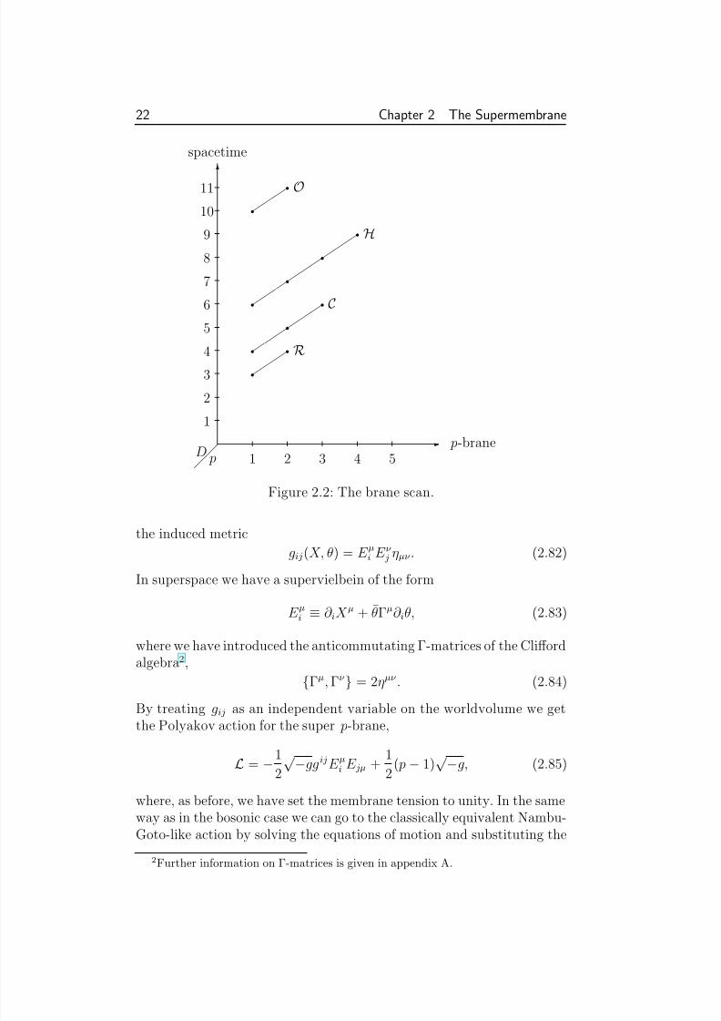
A very fundamental conclusion to be drawn from the above kind of reasoning is that the maximum possible dimension allowed for spacetimeis eleven. If D ≥ 12 then M ≥ 64, for which there are no solutions to(2.79). Likewise the upper limit on the dimensionality of the p-braneis five since (2.79) has no solution for p ≥ 6. The results of the branescan are summarized in figure 2.2. From the figure we can easily see that
1This important symmetry is examined more thoroughly in appendix B.
8/3/2019 Ronnie Jansson- The Membrane Vacuum State
http://slidepdf.com/reader/full/ronnie-jansson-the-membrane-vacuum-state 27/107
2.3 Super p-branes 21
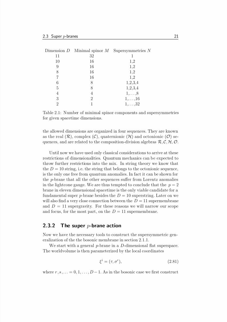
Dimension D Minimal spinor M Supersymmetries N
11 32 110 16 1,29 16 1,28 16 1,27 16 1,26 8 1,2,3,45 8 1,2,3,44 4 1,. . . ,83 2 1,. . . ,162 1 1,. . . ,32
Table 2.1: Number of minimal spinor components and supersymmetriesfor given spacetime dimensions.
the allowed dimensions are organized in four sequences. They are knownas the real (R), complex (C), quaternionic (H) and octonionic (O) se-quences, and are related to the composition-division algebras R, C, H, O.
Until now we have used only classical considerations to arrive at theserestrictions of dimensionalities. Quantum mechanics can be expected tothrow further restrictions into the mix. In string theory we know that
the D = 10 string, i.e. the string that belongs to the octonionic sequence,is the only one free from quantum anomalies. In fact it can be shown forthe p-brane that all the other sequences suffer from Lorentz anomaliesin the lightcone gauge. We are thus tempted to conclude that the p = 2brane in eleven dimensional spacetime is the only viable candidate for afundamental super p-brane besides the D = 10 superstring. Later on wewill also find a very close connection between the D = 11 supermembraneand D = 11 supergravity. For these reasons we will narrow our scopeand focus, for the most part, on the D = 11 supermembrane.
2.3.2 The super p-brane actionNow we have the necessary tools to construct the supersymmetric gen-eralization of the the bosonic membrane in section 2.1.1.
We start with a general p-brane in a D-dimensional flat superspace.The worldvolume is then parameterized by the local coordinates
ξi = (τ, σr), (2.81)
where r,s , . . . = 0, 1, . . . , D − 1. As in the bosonic case we first construct
8/3/2019 Ronnie Jansson- The Membrane Vacuum State
http://slidepdf.com/reader/full/ronnie-jansson-the-membrane-vacuum-state 28/107
22 Chapter 2 The Supermembrane
E
T
D p
p-brane
spacetime
1
2
34
5
6
7
8
9
10
11
1 2 3 4 5
· ·· ·
·· · · ·· ·
R
C
H
O
Figure 2.2: The brane scan.
the induced metricgij(X, θ) = E µi E ν
j ηµν . (2.82)
In superspace we have a supervielbein of the form
E µi ≡ ∂ iX µ + θΓµ∂ iθ, (2.83)
where we have introduced the anticommutating Γ-matrices of the Cliffordalgebra2,
Γµ, Γν = 2ηµν . (2.84)
By treating gij as an independent variable on the worldvolume we getthe Polyakov action for the super p-brane,
L = −1
2
√−ggij E µi E jµ +1
2( p − 1)
√−g, (2.85)
where, as before, we have set the membrane tension to unity. In the sameway as in the bosonic case we can go to the classically equivalent Nambu-Goto-like action by solving the equations of motion and substituting the
2Further information on Γ-matrices is given in appendix A.
8/3/2019 Ronnie Jansson- The Membrane Vacuum State
http://slidepdf.com/reader/full/ronnie-jansson-the-membrane-vacuum-state 29/107
2.3 Super p-branes 23
on-shell metric. For the supermembrane in flat eleven-dimensional target
space this action is
L = −√−g − ijk
1
2∂ iX µ∂ j X ν +
1
2∂ iX µθΓν ∂ jθ
+1
6θΓµ∂ iθθΓν ∂ jθ
θΓµν ∂ kθ. (2.86)
From the Polyakov action we obtain the Euler-Lagrange equations of motion,
∂ i(√−ggijE µ j ) = ijk E ν
j ∂ j θΓµν ∂ kθ, (2.87)
(1 + Γ)gij
/E i∂ jθ = 0, (2.88)where
Γ ≡ ijk
6√−g
E µi E ν j E ρk Γµνρ (2.89)
and Γ2 = 1 (for a proof, see appendix B), thus making 1 ± Γ projectionoperators, eliminating half the spinor components.
The symmetries of the action is:
• Global super-Poincare transformations,
δX µ = aµ + ωµν X ν − Γµθ (2.90)
δθ = 14
ωµν Γµν θ + , (2.91)
where is a constant anticommuting spacetime spinor.
• Local gauge symmetry, in the form of worldvolume reparametriza-tion invariance along a vector field ζ and a fermionic κ-symmetry,
δX µ = ζ i∂ iX µ + κ(1 − Γ)Γµθ (2.92)
δθ = ζ i∂ iθ + (1 − Γ)κ, (2.93)
with κ a 32-component Majorana spinor. Via Noether’s theorem we can
obtain the supercharges (supersymmetry generators)
Q =
d2σJ 0, (2.94)
with the conserved supercurrent being
J i = −2√−ggij /E j θ − ijk
E µ j E ν
k Γµν θ +4
3[Γν θ(θΓµν ∂ jθ)
+ Γµν θ(θΓν ∂ j θ)](E µk − 2
5θΓµν ∂ kθ)
. (2.95)
8/3/2019 Ronnie Jansson- The Membrane Vacuum State
http://slidepdf.com/reader/full/ronnie-jansson-the-membrane-vacuum-state 30/107
24 Chapter 2 The Supermembrane
We conclude this chapter by presenting the supermembrane action
in a curved background space. The action was proposed by Bergshoeff,Sezgin and Townsend in 1987 [28] and investigated extensively later thatyear [29]. The action presented below differ, however, from their actionby a factor 1/3! in the last term due to slightly different conventions.The action is,
S =
d3ξ
−1
2
√−ggijΠai Πb
j ηab +1
2
√−g − 1
3!ijk ΠA
i ΠB j ΠC
k BCBA
,
(2.96)where indices A,B,C are flat super indices and a, b are flat vector indices(A = a, α). The pullback is defined as,
ΠAi = (∂ iZ M )E A
M , (2.97)
with E AM the supervielbein and
E A = dZ M E AM . (2.98)
The 3-form B is the potential to the 4-form H ,
H = dB, (2.99)
with B being defined as
B =1
3!E AE BE C BCB A. (2.100)
The action has two local gauge invariances; local fermionic κ-symmetry(investigated in detail in appendix B), and d = 3 reparametrization in-variance,
δZ M = ηi(ξ)∂ iZ M (2.101)
δgij = ηk∂ kgij + 2∂ (iηkg j)k. (2.102)
8/3/2019 Ronnie Jansson- The Membrane Vacuum State
http://slidepdf.com/reader/full/ronnie-jansson-the-membrane-vacuum-state 31/107
3
The Supermembrane: Spectrumand M-Theory
This chapter has three parts. We begin with a treatment of the linkbetween matrix theory and supermembranes, then move on to investigatethe membrane spectrum. The last part is a brief overview of what hasbecome known as M-theory.
3.1 Supermembranes and matrix theory
In this section we will continue our treatment of the supermembrane andhighlight its connection to matrix theory.
3.1.1 Lightcone gauge and Hamiltonian formalism
As before we enter the lightcone gauge by introducing the standard light-cone coordinates
X ± =1
√2
(X 10
±X 0), (3.1)
and imposing the condition
X +(ξ) = X +(0) + τ ⇐⇒ ∂ iX + = δi0. (3.2)
Transverse coordinates are X (ξ) = X a(ξ), with a = 1, . . . , 9. In completeanalogy for the gamma matrices, we define
Γ± =1√
2(Γ10 ± Γ0). (3.3)
25
8/3/2019 Ronnie Jansson- The Membrane Vacuum State
http://slidepdf.com/reader/full/ronnie-jansson-the-membrane-vacuum-state 32/107
26 Chapter 3 The Supermembrane: Spectrum and M-Theory
The κ-symmetry is gauged fixed by imposing the gauge condition
Γ+θ = 0, (3.4)
thus reducing the number of fermionic degrees of freedom from 32 to 16.After these substitutions the induced metric becomes
grs = ∂ r X · ∂ s X ≡ grs, (3.5)
g0r = ∂ rX − + ∂ 0 X · ∂ r X + θΓ−∂ rθ ≡ ur, (3.6)
g00 = 2∂ 0X − + (∂ 0 X )2 + 2θΓ−∂ 0θ. (3.7)
Furthermore, the metric determinant can be written as,
g ≡ −∆g, (3.8)
with, as before,
g ≡ detgrs, grsgst = δrt , ∆ = −g00 + urgrsus. (3.9)
The lightcone Lagrangian then becomes
L = −
g∆ + rs∂ rX aθΓ−Γa∂ sθ. (3.10)
To obtain the Hamiltonian density we first calculate the canonical mo-menta P , P + and S (conjugate to X , X − and θ):
P =∂ L
∂ (∂ 0 X )=
g
∆
∂ 0 X − urgrs∂ s X
, (3.11)
P + =∂ L
∂ (∂ 0X −)=
g
∆(3.12)
S =∂ L
∂ (∂ 0θ)= −
g
∆Γ−θ. (3.13)
The Hamiltonian density is then
H = P · ∂ 0 X + P +∂ 0X − + S∂ 0θ − L (3.14)
= P 2 + g
2P +− rs∂ rX aθΓ−Γa∂ sθ, (3.15)
and the Hamiltonian itself being the integral of the above density overthe membrane, i.e.,
H =
M
d2σH(σ). (3.16)
8/3/2019 Ronnie Jansson- The Membrane Vacuum State
http://slidepdf.com/reader/full/ronnie-jansson-the-membrane-vacuum-state 33/107
3.1 Supermembranes and matrix theory 27
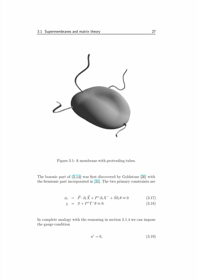
Figure 3.1: A membrane with protruding tubes.
The bosonic part of (3.14) was first discovered by Goldstone [30] withthe fermionic part incorporated in [31]. The two primary constraints are
φr = P · ∂ r X + P +∂ rX − + S∂ rθ ≈ 0 (3.17)
χ = S + P +Γ−θ ≈ 0. (3.18)
In complete analogy with the reasoning in section 2.1.4 we can imposethe gauge condition
ur = 0, (3.19)
8/3/2019 Ronnie Jansson- The Membrane Vacuum State
http://slidepdf.com/reader/full/ronnie-jansson-the-membrane-vacuum-state 34/107
28 Chapter 3 The Supermembrane: Spectrum and M-Theory
and introduce the normalized spatial metric w(σ), and then produce the
membrane momenta
P +0 =
d2σP +, (3.20)
P 0 =
d2σ P , (3.21)
P −0 =
d2σH. (3.22)
The membrane mass then becomes
M2
= d2
σ [ P 2] + g w(σ) − 2P
+
0 rs
∂ rX a
θΓ−
Γa∂ sθ , (3.23)
the prime again indicating the exclusion of the zero modes
X 0 =
d2σ
w(σ) X (σ) (3.24)
θ0 =
d2σ
w(σ)θ(σ). (3.25)
Due to the fact that the bosonic part of (3.23) is
M2 = H = T + V (3.26)
we obtain the potential energy
V =
d2σg =
d2σ det
r,s(∂ r X · ∂ s X ) =
d2σ(rs∂ rX a∂ sX b)2. (3.27)
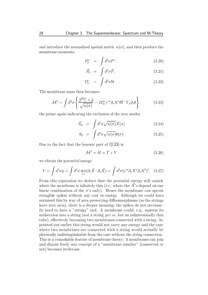
From this expression we deduce that the potential energy will vanishwhere the membrane is infinitely thin (i.e., where the X ’s depend on onelinear combination of the σ’s only). Hence the membrane can sproutstringlike spikes without any cost in energy. Although we could havesurmised this by way of area preserving diffeomorphisms (as the strings
have zero area), there is a deeper meaning; the spikes do not necessar-ily need to have a ”stringy” end. A membrane could, e.g., squeeze itsmidsection into a string (not a string per se, but an infinitesimally thintube), effectively becoming two membranes connected with a string. Aspointed out earlier this string would not carry any energy and the casewhere two membranes are connected with a string would actually bephysically indistinguishable from the case without the string connection.This is a remarkable feature of membrane theory: if membranes can joinand disjoin freely any concept of a ”membrane number” (conserved ornot) becomes irrelevant.
8/3/2019 Ronnie Jansson- The Membrane Vacuum State
http://slidepdf.com/reader/full/ronnie-jansson-the-membrane-vacuum-state 35/107
3.1 Supermembranes and matrix theory 29
Figure 3.2: Physically indistinguishable membranes with different topolo-gies.
3.1.2 Membrane regularization
We will now establish the relation between the APD algebra of the su-permembrane and the N → ∞ limit of a supersymmetric SU (N ) matrixmodel.
We begin by expanding our superspace coordinates into a completeorthonormal set of functions Y A(σ) on the membrane,
X (σ) = X 0 + A
X AY A(σ), (A = 0, 1, 2, . . .) (3.28)
and an analogous basis for the fermionic coordinates θ. For the sake of simplicity we choose Y A to be real. We then introduce the metric ηAB toenable raising and lowering of A , B , . . . indices,
ηABY B(σ) = Y A(σ), (3.29)
where the metric satisfy, as usual,
ηABηBC = δAC . (3.30)

8/3/2019 Ronnie Jansson- The Membrane Vacuum State
http://slidepdf.com/reader/full/ronnie-jansson-the-membrane-vacuum-state 36/107
30 Chapter 3 The Supermembrane: Spectrum and M-Theory
Figure 3.3: Membranes connected by infinitesimally thin tubes.
Normalization of Y A(σ) is done according to the orthogonality relations d2σ
w(σ)Y A(σ)Y B(σ) = δB
A , (3.31)
or, equivalently, d2σ
w(σ)Y A(σ)Y B(σ) = ηAB. (3.32)
Furthermore we need the completeness relation to be fulfilled,
A
Y A(σ)Y A(σ) = 1 w(σ)
δ(σ − σ). (3.33)
This relation is crucial because it allows us to rewrite the Lie bracket inthe new basis,
Y A, Y B = f C AB Y C , (3.34)
with the totally antisymmetric structure constants
f C AB =
d2σ rs∂ rY A∂ sY BY C . (3.35)
8/3/2019 Ronnie Jansson- The Membrane Vacuum State
http://slidepdf.com/reader/full/ronnie-jansson-the-membrane-vacuum-state 37/107
3.1 Supermembranes and matrix theory 31
To regularize the membrane we now truncate the theory by placing an
upper limit Λ on the number of modes indexed by A , B , . . .. The APDgroup is approximated by a finite-dimensional Lie group GΛ whose struc-ture constants are equivalent to the APD structure constants in the limitΛ → ∞. We then get the consistency condition
limΛ→∞
f AB C (GΛ) = f AB C (AP D), (3.36)
for any fixed A,B,C . In the case of spherical membranes [30,32] (a morerecent review can be found in [33]) it was shown that
GΛ = SU (N ) (3.37)
where Λ = N 2 − 1. This result was subsequently generalized to toroidal[34], and then later arbitrary [35], membranes. As we are dealing withSU (N ) matrices we can furthermore replace the Lie bracket with a com-mutator
·, · → [·, ·]. (3.38)
We can elucidate the regularization by working through the exampleof toroidal membranes. We then use the torus coordinates 0 ≤, σ1, σ2 < 2πand define the basis functions
Y m(σ) = ei m·σ, (3.39)
where m = (m1, m2) with m1 and m2 being integers. The weight functionand metric are, respectively,
w(σ) =
1
4π2, (3.40)
ηmn = δm+n. (3.41)
Inserting this metric into the Lie bracket
A, B(σ) ≡ rs w(σ)
∂ rA(σ)∂ sB(σ), (3.42)
will then yield
Y m, Y n = −4π2( m × n)Y m+n. (3.43)
This together with the above metric then gives us the structure constants
f mnk = −4π2( m × n)δm+n+k. (3.44)
8/3/2019 Ronnie Jansson- The Membrane Vacuum State
http://slidepdf.com/reader/full/ronnie-jansson-the-membrane-vacuum-state 38/107
32 Chapter 3 The Supermembrane: Spectrum and M-Theory
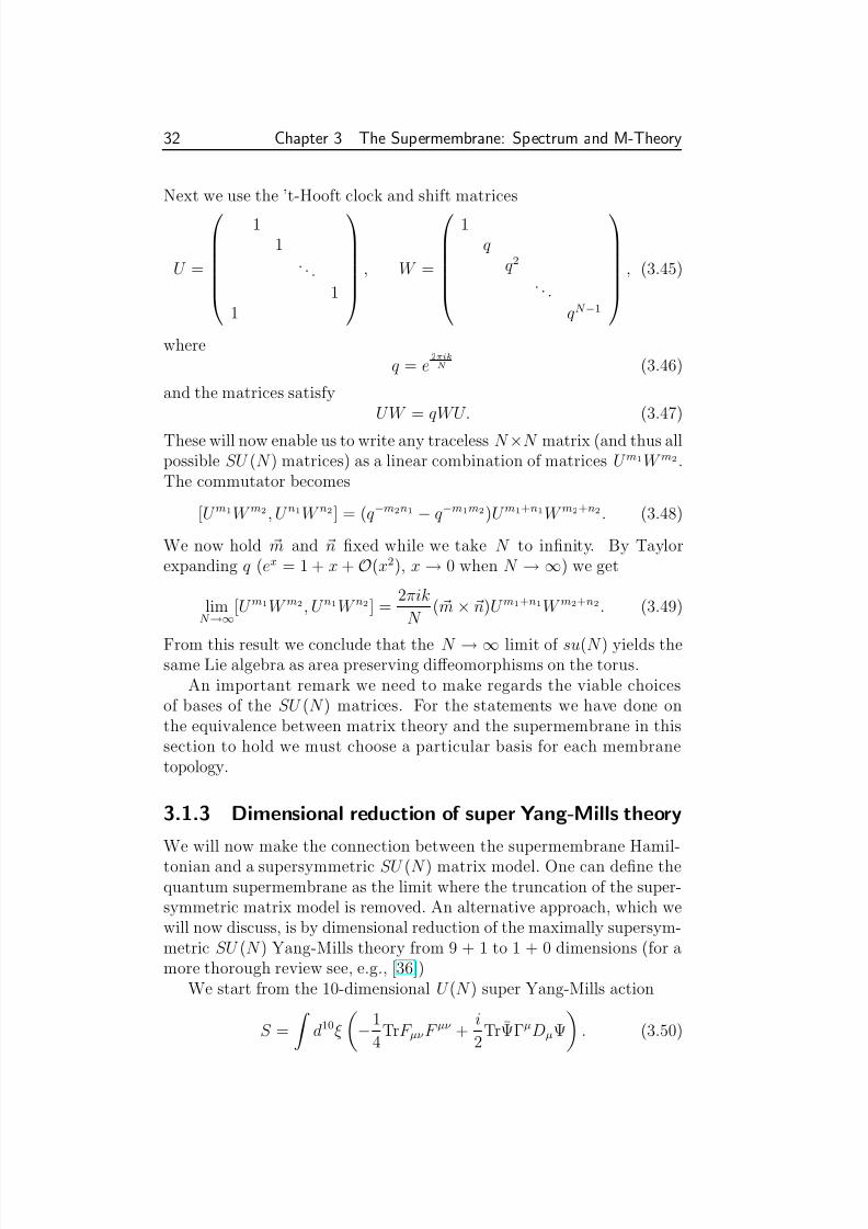
Next we use the ’t-Hooft clock and shift matrices
U =
1
1. . .
11
, W =
1
qq2
. . .
qN −1
, (3.45)
whereq = e
2πikN (3.46)
and the matrices satisfyUW = qWU. (3.47)
These will now enable us to write any traceless N ×N matrix (and thus allpossible SU (N ) matrices) as a linear combination of matrices U m1W m2 .The commutator becomes
[U m1W m2 , U n1W n2] = (q−m2n1 − q−m1m2)U m1+n1W m2+n2 . (3.48)
We now hold m and n fixed while we take N to infinity. By Taylorexpanding q (ex = 1 + x + O(x2), x → 0 when N → ∞) we get
limN →∞
[U m1W m2, U n1W n2] =2πik
N ( m × n)U m1+n1W m2+n2. (3.49)
From this result we conclude that the N → ∞ limit of su(N ) yields thesame Lie algebra as area preserving diffeomorphisms on the torus.
An important remark we need to make regards the viable choicesof bases of the SU (N ) matrices. For the statements we have done onthe equivalence between matrix theory and the supermembrane in thissection to hold we must choose a particular basis for each membranetopology.
3.1.3 Dimensional reduction of super Yang-Mills theory
We will now make the connection between the supermembrane Hamil-
tonian and a supersymmetric SU (N ) matrix model. One can define thequantum supermembrane as the limit where the truncation of the super-symmetric matrix model is removed. An alternative approach, which wewill now discuss, is by dimensional reduction of the maximally supersym-metric SU (N ) Yang-Mills theory from 9 + 1 to 1 + 0 dimensions (for amore thorough review see, e.g., [36])
We start from the 10-dimensional U (N ) super Yang-Mills action
S =
d10ξ
−1
4TrF µν F µν +
i
2TrΨΓµDµΨ
. (3.50)
8/3/2019 Ronnie Jansson- The Membrane Vacuum State
http://slidepdf.com/reader/full/ronnie-jansson-the-membrane-vacuum-state 39/107
3.1 Supermembranes and matrix theory 33
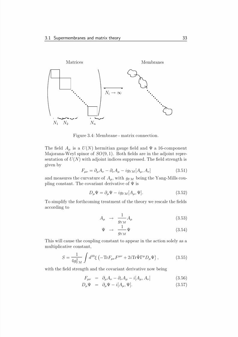
Matrices Membranes
E'
N i → ∞
N 1 N 2 N n
Figure 3.4: Membrane - matrix connection.
The field Aµ is a U (N ) hermitian gauge field and Ψ a 16-componentMajorana-Weyl spinor of SO(9, 1). Both fields are in the adjoint repre-sentation of U (N ) with adjoint indices suppressed. The field strength isgiven by
F µν = ∂ µAν − ∂ ν Aµ − igY M [Aµ, Aν ] (3.51)
and measures the curvature of Aµ, with gY M being the Yang-Mills cou-pling constant. The covariant derivative of Ψ is
DµΨ = ∂ µΨ − igY M [Aµ, Ψ]. (3.52)
To simplify the forthcoming treatment of the theory we rescale the fieldsaccording to
Aµ → 1
gY M Aµ (3.53)
Ψ → 1
gY M Ψ (3.54)
This will cause the coupling constant to appear in the action solely as amultiplicative constant,
S =1
4g2Y M
d10ξ
−TrF µν F µν + 2iTrΨΓµDµΨ
, (3.55)
with the field strength and the covariant derivative now being
F µν = ∂ µAν − ∂ ν Aµ − i[Aµ, Aν ] (3.56)
DµΨ = ∂ µΨ − i[Aµ, Ψ]. (3.57)
8/3/2019 Ronnie Jansson- The Membrane Vacuum State
http://slidepdf.com/reader/full/ronnie-jansson-the-membrane-vacuum-state 40/107
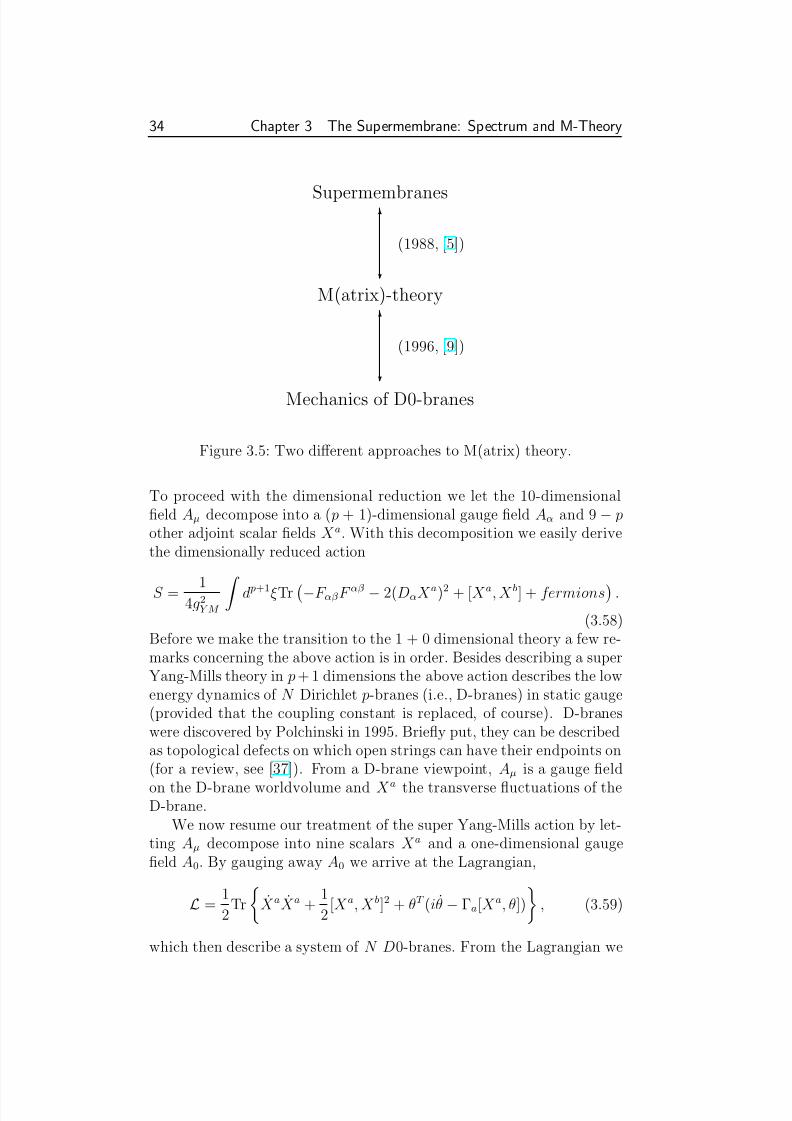
34 Chapter 3 The Supermembrane: Spectrum and M-Theory
Supermembranes
(1988, [5])
c
T
M(atrix)-theory
(1996, [9])
c
T
Mechanics of D0-branes
Figure 3.5: Two different approaches to M(atrix) theory.
To proceed with the dimensional reduction we let the 10-dimensionalfield Aµ decompose into a ( p + 1)-dimensional gauge field Aα and 9 − pother adjoint scalar fields X a. With this decomposition we easily derivethe dimensionally reduced action
S = 14g2Y M
d p+1ξTr −F αβ F αβ − 2(DαX a)2 + [X a, X b] + fermions .
(3.58)Before we make the transition to the 1 + 0 dimensional theory a few re-marks concerning the above action is in order. Besides describing a superYang-Mills theory in p + 1 dimensions the above action describes the lowenergy dynamics of N Dirichlet p-branes (i.e., D-branes) in static gauge(provided that the coupling constant is replaced, of course). D-braneswere discovered by Polchinski in 1995. Briefly put, they can be describedas topological defects on which open strings can have their endpoints on(for a review, see [37]). From a D-brane viewpoint, Aµ is a gauge field
on the D-brane worldvolume and X a the transverse fluctuations of theD-brane.
We now resume our treatment of the super Yang-Mills action by let-ting Aµ decompose into nine scalars X a and a one-dimensional gaugefield A0. By gauging away A0 we arrive at the Lagrangian,
L =1
2Tr
X aX a +
1
2[X a, X b]2 + θT (iθ − Γa[X a, θ])
, (3.59)
which then describe a system of N D0-branes. From the Lagrangian we
8/3/2019 Ronnie Jansson- The Membrane Vacuum State
http://slidepdf.com/reader/full/ronnie-jansson-the-membrane-vacuum-state 41/107
3.2 The (super)membrane spectrum 35
then easily derives the corresponding matrix Hamiltonian,
H =1
2Tr
P aP a − 1
2[X a, X b]2 + θT Γa[X a, θ]
. (3.60)
This Hamiltonian is the dimensional reduction of the maximally super-symmetric SU (N ) Yang-Mills Hamiltonian from 9+ 1 to 0+1 dimensionsand also the truncated model of the supermembrane. The above Hamil-tonian and Lagrangian also play an important role in M-theory by wayof the BFSS conjecture, which we will discuss further in section 3.3.5.
3.2 The (super)membrane spectrumThe matter as to whether the bosonic and supersymmetric membranehave continuous or discrete spectra is not without its surprises nor im-plications, some of which we will discuss now.
3.2.1 The bosonic membrane spectrum
The bosonic Hamiltonian belongs to the group of Hamiltonians wherethe volume
( p,q)
| p2 + V (q)
≤E
(3.61)
is infinite for some E < ∞. For such cases the standard wisdom [2]proclaims that the spectrum is not purely discrete. In the opposite casewhere the volume is always finite the same wisdom dictates that thespectrum is purely discrete. Wisdom, however, is no match for properphysics and while the latter wisdom holds true, the former does not.
If we express the quantum and classical partition functions as
Z q(t) = Tr(e−tH ) (3.62)
Z cl(t) =1
(2π)ν dν p dν q e−t( p2+V (q)), (3.63)
we have the Golden-Thompson inequality
Z q(t) ≤ Z cl(t). (3.64)
Our lightcone membrane Hamiltonian can be re-written [38] and ex-pressed as
H =
d2σ
P iP i +
i<j
(X iX j )2
, i, j = 1, 2, . . . , D − 2. (3.65)
8/3/2019 Ronnie Jansson- The Membrane Vacuum State
http://slidepdf.com/reader/full/ronnie-jansson-the-membrane-vacuum-state 42/107
36 Chapter 3 The Supermembrane: Spectrum and M-Theory
If we restrict ourselves to the case of D = 4 we obtain (after a slight
change in notation) the Hamiltonian
H 1 = − ∂ 2
∂x2− ∂ 2
∂y2+ x2y2. (3.66)
In [2] no less than five proofs of H 1 having a discrete spectrum are given.We will, however, only concern ourselves with the simplest one. Thisproof is derived from the zero point harmonic oscillator,
− d2
dq2+ ω2q2 ≥|ω | . (3.67)
By treating y as a complex number we get
− d2
dx2+ x2y2 ≥|y | . (3.68)
By using this and the symmetry between x and y we easily derive theinequality
H 1 = − d2
dx2− d2
dy2+ x2y2 (3.69)
=1
2 − d2
dx2+ x2y2
+1
2 − d2
dy2+ x2y2
−1
2
d2
dx2+
d2
dy2
(3.70)
≥ 1
2(−∆+ |x | + |y |) = H 2, (3.71)
and show that H 2 has a discrete spectrum, since
Tr(e−tH 2) = [1 + O(1)]1
(2π)2
d2 pdxdyetp2−t|x|−t|y| (3.72)
= ct−3[1 + O(1)]. (3.73)
This, of course, means that
Z q = Tr(e−tH 1) ≤ ct−3. (3.74)
It should be noted, however, that this is a very poor approximation andthe true relation [2] should be
Tr(e−tH 1) ≤ O(t−3/2 ln t). (3.75)
Nonetheless, our purpose was only to prove the discreteness of the spec-trum, which we have now done.
8/3/2019 Ronnie Jansson- The Membrane Vacuum State
http://slidepdf.com/reader/full/ronnie-jansson-the-membrane-vacuum-state 43/107
3.2 The (super)membrane spectrum 37
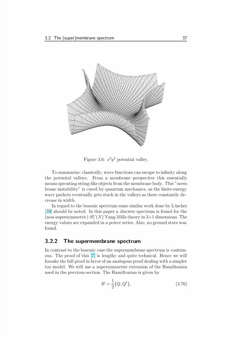
Figure 3.6: x2y2 potential valley.
To summarize: classically, wave functions can escape to infinity along
the potential valleys. From a membrane perspective this essentiallymeans sprouting string-like objects from the membrane body. This ”mem-brane instability” is cured by quantum mechanics, as the finite-energywave packets eventually gets stuck in the valleys as these constantly de-crease in width.
In regard to the bosonic spectrum some similar work done by Luscher[39] should be noted. In this paper a discrete spectrum is found for the(non-supersymmetric) SU (N ) Yang-Mills theory in 3+1 dimensions. Theenergy values are expanded in a power series. Also, no ground state wasfound.
3.2.2 The supermembrane spectrum
In contrast to the bosonic case the supermembrane spectrum is continu-ous. The proof of this [7] is lengthy and quite technical. Hence we willforsake the full proof in favor of an analogous proof dealing with a simplertoy model. We will use a supersymmetric extension of the Hamiltonianused in the previous section. The Hamiltonian is given by
H =1
2Q, Q†, (3.76)
8/3/2019 Ronnie Jansson- The Membrane Vacuum State
http://slidepdf.com/reader/full/ronnie-jansson-the-membrane-vacuum-state 44/107
38 Chapter 3 The Supermembrane: Spectrum and M-Theory
with the supercharges being
Q = Q† =
−xy i∂ x + ∂ yi∂ x − ∂ y xy
, (3.77)
with x and y, of course, being the normal Cartesian coordinates. TheHamiltonian then becomes
H =
−∆ + x2y2 x + iyx − iy −∆ + x2y2
, (3.78)
and we immediately recognize the bosonic Hamiltonian in the diagonal
elements. The effect of the fermionic parts, however, will be crucial:the off-diagonal terms will make a negative energy contribution and thusnegating the confining properties evident in the bosonic theory. More tothe point, it will be possible to construct wave packets that can escapeto infinity along the coordinate axis (i.e., the potential valleys) withouta corresponding infinite cost of energy. The easiest way to show this isto explicitly construct said wave packets.
To proceed, we choose to study the y = 0 direction and start withthe ansatz
ψt(x, y) = χ(x − t)ϕ0(x, y)ξF , (3.79)
where χ(x) is a smooth function with compact support such that χ van-ishes unless x is of order t, and
ξF =1√
2
1
−1
. (3.80)
If we increase the parameter t the wave packet is translated in the x-direction. Furthermore, as t → ∞ the wave packet moves to infinityalong the y = 0 valley. The spinor ξF was chosen to maximize thenegative energy contribution of the wave packet, and we have
ξT
F HξF = H bosonic − x. (3.81)
Moreover, the fermionic contribution to the energy expectation value of the state ψt turns out to be −t + O(1) for large t (χ dominates whent becomes large). This negative contribution is exactly what we needto cancel the bosonic groundstate energy of a harmonic oscillator in they = 0 valley. Next we choose a wave function of such an oscillator,
ϕ0(x, y) =
| x |π
1
4
e−1
2|x|y2. (3.82)
8/3/2019 Ronnie Jansson- The Membrane Vacuum State
http://slidepdf.com/reader/full/ronnie-jansson-the-membrane-vacuum-state 45/107
3.3 M-theory 39
For ν = 0, 1, 2 we then have
limt→∞
(ψt, H ν ψt) =
dx χ(x)∗(−∂ 2x)ν χ(x), (3.83)
which is finite. In other words, we are allowed to shift the wave packetto infinity without the energy ever going off to infinity.
To finalize this treatment let us choose an arbitrary energy E ≥ 0 andε > 0. Next we choose χ(x) such that
χ = 1, (−∂ 2x − E )χ 2<ε
2. (3.84)
For large t we will then have
χt = 1, (H − E )ψt 2< ε. (3.85)
Hence, as ε can be arbitrarily small, we have proved that indeed any valueE ≥ 0 is an energy eigenvalue of the Hamiltonian (3.78), which then havea continuous spectrum. We should end with a remark concerning the fullmembrane case: here the wave functions can escape to infinity alongdirections corresponding to the generators of the Cartan subalgebra of the algebra corresponding to the SU (N ) group.
3.2.3 A second quantized theory
To recapitulate, we have shown that the bosonic membrane has, clas-sically, a continuous spectrum and, quantum mechanically, a discretespectrum. If supersymmetry is then switched on the spectrum is againcontinuous. This is (was) bad news for the first quantization of the the-ory, which by its very nature should be discrete. In fact, this causedthe membrane community to dishearten and disperse into, at the time,more interesting research areas. A few years later, around the time of theBFSS conjecture (see section 3.3.5), there was a revival of membrane the-ory and the previously fatal flaw, the continuous spectrum, was realizedto be no nothing but a blessing in disguise. The simple, yet profound,
realization was to interpret the continuous spectrum of the quantum su-permembrane not as a hindrance to first quantize the theory, but as asign that the theory is second quantized to begin with . Membrane theorythus deals with ”multi-membrane” states from the very outset.
3.3 M-theory
In this section we will try to swiftly cover a large part of what is nowcalled M-theory. The treatment will differ from the rest of the thesis in
8/3/2019 Ronnie Jansson- The Membrane Vacuum State
http://slidepdf.com/reader/full/ronnie-jansson-the-membrane-vacuum-state 46/107
40 Chapter 3 The Supermembrane: Spectrum and M-Theory
that it will be of much lesser technical nature. The width of the content
is rivaled only by the lack of depth in the treatment.For more in-depth treatments of string theory, see [40] and [41]; du-
ality, [42]; M-theory, [43] and [42].
3.3.1 Supergravity
Local supersymmetry actually predicts (super)gravity by demanding theexistence of the spin 2 graviton and its supersymmetric partner, the spin3/2 gravitino. In other words, if general relativity had not been discov-ered at the time of local supersymmetry, we would have been forced to
invent it. What’s more, supergravity includes the symmetries of bothgravity and the grand unified forces, thus making it a candidate for aTheory of Everything. Like we showed for p-branes in chapter 2 super-gravity imposes an upper limit of 11 on the number of spacetime dimen-sions. It is furthermore in this dimensionality that supergravity takesits most elegant form. A serious problem of supergravity, however, is itsnon-chirality. Nature is chiral, and as Witten among others showed it isimpossible to generate a chiral theory from a non-chiral one (ironically,it was Witten who later evaded this no-go theorem). Another problemis the fact that general relativity is non-renormalizable. This in itself is not a disaster, a renormalizable theory containing both massless and
massive particles can be disguised as a non-renormalizable theory if weremove the massive particles by using their equations of motion. Theremaining non-renormalizable theory containing only massless particlesis then fully applicable at energies lower than m pc2, where m p is the massscale associated with the excluded massive particles. If we would wantto describe gravity at higher energies, a more fundamental theory withmassive particles included would be needed. The mass m p, we associatewith any quantum theory of gravity and is derived from the fundamentalconstants of gravity (G), special relativity (c) and quantum mechanics(h), thus yielding the relevant energy scale,
E p = m pc2 =
hc
Gc2 ≈ 1016 TeV. (3.86)
This is the planck energy, and it is in a word, huge. Current energiesavailable at CERN have just reached the TeV range.
In conclusion, the theory we are looking for should contain super-symmetry, massive particles and reduce to Einstein’s theory of gravity atlow energies. However, we know all the supersymmetric quantum fieldtheories and no one of them fulfill those requirements.
8/3/2019 Ronnie Jansson- The Membrane Vacuum State
http://slidepdf.com/reader/full/ronnie-jansson-the-membrane-vacuum-state 47/107
3.3 M-theory 41
3.3.2 Strings
String first surfaced in theoretical physics in the 1960s as a model of hadrons. The theory suffered from various severe problems and wasabandoned in the early 70s in favor of the hugely successful quantumchromodynamics. A smaller group of physicists remained with stringtheory, however, and eventually managed to solve, sidestep or surmountmany of the problems guilty of having condemned string theory to theperiphery of respectable research. In addition, string theory was nowconsidered not simply a model of strong interactions, but as a candidatefor the Theory of Everything. In 1984, in what has become known asthe (first) superstring revolution, string theory entered mainstream the-
oretical physics. At this time it was shown that certain string theories(there were five) were free of anomalies. In addition, ways to compactifythe ”excess” dimensions of 10-dimensional superstring theories by way of Calabi-Yau manifolds were also found.
In string theory the length scale is determined by the string tensionT = (2πα)−1, where
√α has dimension of length. For string theory to
describe the strength of the gravitational force correctly, we must set√
α ∼ 10−35m. (3.87)
Consequently, this is also the typical length scale of the strings.
When we want to construct a fully consistent string theory, involvingboth bosonic and fermionic degrees of freedom, we arrive at no less thanfive different consistent theories, all in ten spacetime dimensions. Theyare called the type IIA, type IIB, Type I, E 8 × E 8 heterotic and SO(32)heterotic string theories. We hereby give a short description of each of these theories.
• Type IIA and IIB string theories:. The field description of these twotheories contain eight scalar fields (bosons) and sixteen Majorana-Weyl spinors (fermions). Bosonic and fermionic degrees of free-dom remains matched as the sixteen Majorana-Weyl spinors are
equivalent to eight Majorana spinors. From the chiral nature of the fermions we will differentiate between their handedness by re-ferring to them as left- and right-moving (eight of each). Thesestring theories contain closed strings exclusively, and are thus sub-
ject to periodic boundary conditions for the bosonic degrees of free-dom. The fermions may have either periodic or anti-periodic con-ditions, which is referred to as Ramond boundary conditions (R)and Neveu-Schwarz boundary conditions (NS), respectively. Con-sistency then requires four seperate classes of states in the spec-trum: R-R, where both left- and right-moving fermions are subject
8/3/2019 Ronnie Jansson- The Membrane Vacuum State
http://slidepdf.com/reader/full/ronnie-jansson-the-membrane-vacuum-state 48/107
42 Chapter 3 The Supermembrane: Spectrum and M-Theory
to periodic boundary conditions. The other sectors are, of course,
NS-NS, R-NS and NS-R. The next step is to make a so-called GSOprojection. In essence, removing all but about a fourth of the states,keeping the states with an even number of left-moving fermions andan even number of right-moving fermions. The A and B variant of type II string theory arise from the fact that we can choose eitheran even or odd fermion number to the ground state. In type IIAstring theory the GSO projection in the left-moving direction arenot the same as in the right-moving direction. In type IIB the GSOprojections are identical for both directions.
The supersymmetry algebra of type IIA is the non-chiral N = 2
superalgebra, while type IIB have the chiral N = 2 superalgebra.Both consist of 32 supersymmetry generators.
• The heterotic string theories: As with type II string theories theseare closed and oriented strings. Although they both have eightscalar fields, they have, unlike the type II string, eight right-movingMajorana-Weyl fermions and 32 left-moving Majorana-Weyl fermions.Heterotic strings are divided into sectors according to their Neveu-Schwarz and Ramond boundary conditions and then GSO pro-
jected, in a similar (but not identical) way to type II strings. Theresulting consistent string theories are the SO(32) heterotic and
E 8 × E 8 heterotic string theories; their names reflecting their re-spective gauge groups. Their common superalgebra is the N = 1chiral supersymmetry algebra, which has 16 real generators.
• Type I string theory: In contrast to the other four string theo-ries, the type I theory contains unoriented, both open and closed,strings. Open strings of course cannot have periodic boundaryconditions and are instead subjected to Neumann boundary condi-tions. Furthermore is type I string theory invariant under world-sheet parity transformation, a symmetry that exchanges left- andright-moving sectors. Like the heterotic string, the type I spectrum
is invariant under the N = 1 chiral superalgebra.
3.3.3 Duality
Duality is an extremely valuable tool and was to a large part responsibleof unifying the five different string theories under the common bannerof M-theory. What we have said previously about string theory was inregard of the perturbative regime only. However, duality manages tobridge the gap to the non-perturbative region. We will touch briefly onthe three principal dualities:

8/3/2019 Ronnie Jansson- The Membrane Vacuum State
http://slidepdf.com/reader/full/ronnie-jansson-the-membrane-vacuum-state 49/107
3.3 M-theory 43
•T-duality: a perturbative duality relating distances.
• S-duality: a non-perturbative duality relating strong and weak cou-pling.
• U-duality: a duality of dualities relating T- and S-duality to eachother.
If we compactify a string theory on a circle of radius R we would get thenormal so-called Kaluza-Klein modes quantized according to
p =n
R, (3.88)
where n is an integer. However, as we are dealing with strings and notparticles we will have additional modes corresponding to a closed stringwrapped around the circle, with modes
p = mR, (3.89)
where m is the number of times the string has wound around the circle.Ergo, the left- and right-moving modes are
( pL, pR) = n
2R+ mR,
n
2R− mR
. (3.90)
Thus the mass spectrum for M2 is invariant under
R ←→ 1
2R, (3.91)
if we also make the exchange n ↔ m. Hence the string seem to exhibitthe same physics if dimensionally reduced to a circle of minuscule size asto one of titanic proportions. This invariance is the essence of T-dualityand in fact yields an equivalence between type IIA and type IIB stringtheory as well as an equivalence between the two heterotic strings.
S-duality, on the other hand, relates strong coupling to weak cou-
pling, and vice versa. As such, it is a very powerful tool and enablesone to use perturbation theory to probe previously barred regions of atheory. More importantly, S-duality, gives a correspondence between 10-dimensional string theories and 11-dimensional M-theory (the name, M-theory, have been rather abused and can mean either the 11-dimensionalnon-perturbative extension of string theory, or the entire theory formerlyknown as ”string theory”; this thesis will abuse the name further and useit in both cases interchangeably and letting the context decide its mean-ing). M-theory is S-dual to type IIA string theory and its strong couplinglimit (gs → ∞) when M-theory is compactified on a circle, S 1 [4] (see
8/3/2019 Ronnie Jansson- The Membrane Vacuum State
http://slidepdf.com/reader/full/ronnie-jansson-the-membrane-vacuum-state 50/107
44 Chapter 3 The Supermembrane: Spectrum and M-Theory
also [44]). Furthermore, M-theory reduces to the E 8
×E 8 heterotic string
when compactified on a line segment, S 1/Z2. S-duality also connects theSO(32) heterotic string with the type I string. A special case of S-dualityconcerns type IIB, which in fact is self-dual and thus relates the differentregions of the moduli space within the same theory.
The third important duality is U-duality, which connects T- and S-duality to each other. If a string exhibits T-duality the U-dual stringwould exhibit S-duality, and vice versa. This put the, at the time, con-
jectured S-duality on a firm footing as it was shown to be equivalent tothe well-established T-duality.
3.3.4 M-theoryWhat has become known as the second superstring revolution was ignitedby a celebrated talk in 1995 by Edward Witten. The five string theorieswere now firmly unified by the different dualities. A M(other) theoryliving in 11-dimensional spacetime with 11 dimensional supergravity asthe low-energy limit and interconnected with all the five string theoriesnow became the accepted starting point for further research. M-theory(in the broad sense of the word) was the name given to this vast theory,and is summarized in figure 3.7. The link between type I and type IIB, inthe figure denoted by Ω, is an ”orientifold projection”. Going from type
IIB we make an orientation reversal, i.e., σ → −σ. When the smokeclears we are left with unoriented closed strings and unoriented openstrings with an SO(32) gauge symmetry: Type I string theory.
3.3.5 The BFSS conjecture
Despite the properties we have mentioned M-theory must have, any con-crete formulation of the theory has not been done. An attempt at thiswas made by Banks, Fishler, Shenker and Susskind (BFSS) in 1996 witha bold conjecture [45] suggesting that, ”M-theory, in the lightcone frame,is exactly described by the large N limit of a particular supersymmet-
ric matrix quantum mechanics”. More specifically, the matrix quantummechanics consists of N D0-branes. From section 3.1.3 we know thatthe dynamics of such a system of branes are described by the dimension-ally reduced U (N ) super Yang-Mills Hamiltonian from 9 + 1 to 0 + 1dimensions. A D-brane has the mass
M =ms
gs, (3.92)
where ms is the mass scale of type IIA string theory. Having compactifiedthe 11-dimensional theory on a circle of radius R, the following relation
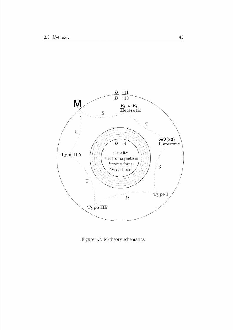
8/3/2019 Ronnie Jansson- The Membrane Vacuum State
http://slidepdf.com/reader/full/ronnie-jansson-the-membrane-vacuum-state 51/107
3.3 M-theory 45
M
Type I
Type IIA
Type IIB
E 8 × E 8Heterotic
SO(32)Heterotic
T
T
S
S
S
Ω
GravityElectromagnetism
Strong forceWeak force
D = 4
D = 10D = 11
Figure 3.7: M-theory schematics.
8/3/2019 Ronnie Jansson- The Membrane Vacuum State
http://slidepdf.com/reader/full/ronnie-jansson-the-membrane-vacuum-state 52/107
46 Chapter 3 The Supermembrane: Spectrum and M-Theory
holds (up to numerical pre-factors),
gs = Rms. (3.93)
We thus deduce that M = 1/R, which prompts us to interpret the braneas the first Kaluza-Klein excitation of the 11-dimensional supergravitymultiplet on the circular dimension. The spatial coordinates of the sys-tem of D0-branes are then represented by N × N matrices. There mightbe higher order corrections, but these are then suppressed by going tothe infinite momentum frame. This frame is reached by letting the mo-mentum
p11 =N
R
(3.94)
go to infinity at the same time as R does so. The BFSS conjecture isthat M-theory is described exactly and non-perturbatively by the N →∞ infinite momentum frame of N D0-branes. The N → ∞ limit isof course troublesome and perhaps also unnecessary; Susskind made afurther conjecture [46] in 1997, suggesting that the BFSS conjecture wasvalid even for finite N .
Since its birth the BFSS conjecture has received much attention andbeen intensely scrutinized. More evidence for its validity has been pre-sented, but perhaps more importantly, so has evidence for the opposite.For instance, in the aptly named article ”Why matrix theory is hard” [47]the authors show a possible contradiction arising from the BFSS conjec-ture. At any rate, the last word has not been said and matrix theoryremains an exciting topic in M-theory.
For further information and references on matrix theory and the BFSSconjecture, see [48] and [49].
8/3/2019 Ronnie Jansson- The Membrane Vacuum State
http://slidepdf.com/reader/full/ronnie-jansson-the-membrane-vacuum-state 53/107
4
The Membrane Vacuum StateIn this chapter we will mainly investigate the ground state of a supersym-metric SU (2) matrix model. This is a natural starting point in the searchfor the membrane vacuum state due to the connection between the su-permembrane and the large N limit of SU (N ) matrix models. The bulkof the treatment will deal with such an SU (2) invariant ground state,whose asymptotic form we will derive; asymptotic in this case meaningfar away from the center of the potential.
4.1 Overview and preliminaries
This section will present a short chronological overview of the researchthat has been done regarding membrane ground states thus far. Asa precursor to the higher-dimensional case presented later we will alsoapply our method of finding a vacuum state on a two-dimensional toymodel.
4.1.1 Current state of affairs
The search for the membrane vacuum state spans about twenty yearsof research and a large number of articles. We will here attempt tooutline the research done (and not done) so far. Invariably, this willfor the most part be a review of the tour de force of Jens Hoppe andcollaborators: [5, 50, 51,52,53, 54, 55, 10, 56, 57,58,59, 60, 61].
In 1984, Claudson and Halpern [6] published their work on supersym-metric ground state wave functions where they investigated the viabilityof constructing such states for many different kinds of supersymmetricHamiltonians. The first attempt at constructing a ground state wave
47
8/3/2019 Ronnie Jansson- The Membrane Vacuum State
http://slidepdf.com/reader/full/ronnie-jansson-the-membrane-vacuum-state 54/107
48 Chapter 4 The Membrane Vacuum State
function specifically for the membrane was conducted by de Wit, Hoppe
and Nicolai in their seminal paper [5] in 1988. Their analysis concernedusing truncations of the supermembrane. They showed for two differenttruncations the absence of a zero energy ground state. They concludedthat, while leaning towards a massive ground state, more work on thesubject was needed. Quite a few years later [50] Hoppe slightly extendedthis earlier work, by commentating on some subtleties in the original pa-per and also showing the lack of a (real) zero energy ground state in thesimplest case of a supermembrane matrix model (SU (2) gauge invariantsupermembrane in D = 4 spacetime). Then in a subsequent paper [51]it was firmly proven that a normalizable zero mass ground state did notexist in the SU (2), D = 4 case. Later the same year Hoppe, in a trioof papers published at a machine-gun pace, made use of another methodto approach the ground state problem. In the first paper [52] he provesthat no solution exists for the case where D = 4, SU (N ) with N odd.He also outlines an analogous model for the more interesting case of 11 dimensions, which is continued in the following paper by obtainingbosonic solutions to the equations Q†
β ψ = 0. The third paper further in-vestigates the 11-dimensional case and tentatively constructs zero energystates. A few months later, in the end of 1997, Halpern and Schwartz [62]used a generalized Hamiltonian Born-Oppenheimer formulation to de-rive asymptotic, normalizable zero energy solutions of the Schrodinger
equation of SU (2) matrix theory corresponding to the 11-dimensionalsupermembrane. Among the ground state candidates found one wasSpin(9) invariant, a property whose significance will become clear later.The result obtained by their rather cumbersome calculation was laterreproduced by Graf and Hoppe [55] with a simpler approach using thesupercharges (containing first order derivatives) instead of the Hamil-tonian (containing second order derivatives). The asymptotic groundstate was SU (2) and SO(9) invariant and determined to leading andsub-leading order from a perturbative expansion of the 16 superchargesQβ = Q
(0)β + Q
(1)β + . . .. In a follow-up paper [10] in 1999 a more gen-
eral theorem was given regarding the states satisfying Qβ ψ = 0 of the
supersymmetric matrix models corresponding to supermembranes in di-mensions D = 4, 5, 7, 11. It is explicitly shown that the 11-dimensionalcase is the only case with a square-integrable SU (2)×Spin(D−2) invari-ant asymptotic ground state wave function, the form of which was alsogiven. The theorem along with its proof will be treated in detail in sec-tion 4.2 and 4.3, respectively. Some months after this paper Hoppe andcollaborators [56] started to investigate the SU (3) invariant zero energystate, an investigation continued in [57] and culminated in [58].
In 2001, Graf, Hasler and Hoppe [59] resolved the issue whether the
8/3/2019 Ronnie Jansson- The Membrane Vacuum State
http://slidepdf.com/reader/full/ronnie-jansson-the-membrane-vacuum-state 55/107
4.1 Overview and preliminaries 49
supersymmetric x2y2 potential allows for zero energy ground states or
not. A similar calculation will also be presented in the next section.In 2002, striving to go beyond the SU (2) and SU (3) case, Hasler andHoppe attempt in [60] to generalize the previous model to include SU (N )invariance. They show that, for all N > 1, when the eigenvalues of the matrices in the matrix model become large and well separated fromeach other the vacuum state wave function factorizes into a product of supersymmetric harmonic oscillator wave functions and an additionalwave function that will be annihilated by a certain supercharge. Then inthe last relevant paper [61] to date, the same authors prove that the zeroenergy states for reduced super Yang-Mills theory in d + 1 dimensionswith d = 2, 3, 5, 9 (the dimension d corresponds to a supermembraneliving in D dimensions according to D = d + 2) is necessarily Spin(d)invariant.
To summarize the current state of this field, we quote this last paper:”The general belief, partially proven, is that for d = 2, 3, 5 no zero energystate exists and that for d = 9 there exists a unique ground state”.
4.1.2 A toy model ground state
In this section we will investigate the possibility of normalized groundstate of a simple two-dimensional model. The supercharge and Hamilto-
nian are similar to the ones used in the toy model of the supermembrane;they are,
Q = i
∂ x ∂ y + xy
∂ y − xy −∂ x
, (4.1)
and
H = (−∂ 2x − ∂ 2y + x2y2) 1 +
x −y
−y −x
, (4.2)
respectively. We are by now familiar with the characteristics and impli-cations of the bosonic potential, x2y2, and hence abstain from any furthercomments on the potential. It should be duly noted, however, that while
the Hamiltonian is simple, the question whether it admits a normalizableground state, is not. In fact, this question remained unsolved for morethan ten years and was given a resolution only recently. The argumentis the following; an approximate solution to
QΨ = 0, (4.3)
when x → +∞ is
Ψ0 = e−xy2
2
01
. (4.4)
8/3/2019 Ronnie Jansson- The Membrane Vacuum State
http://slidepdf.com/reader/full/ronnie-jansson-the-membrane-vacuum-state 56/107
50 Chapter 4 The Membrane Vacuum State
We use this function as the first term in the asymptotic expansion
Ψ = x−κ(Ψ0 + Ψ1 + . . .). (4.5)
We also expand the supercharge in powers of x, as
Q =∞
n=0
Q(n), (4.6)
where n denotes the different powers of x. In our toy model case thesupercharge (4.1) is just the sum of two terms. We have,
Q(0) = i ∂ x 0
0 −∂ x (4.7)
Q(1) = i
0 ∂ y − xy
∂ y − xy 0
. (4.8)
Equation (4.3) now becomes
QΨ =
0 ∂ y + xy
∂ y − xy 0
+
∂ x 00 −∂ x
x−κ(Ψ0 + . . .)
= 0
This equation is equivalent to a set of equations for n = 0, 1, . . .. Bymatching powers of x we get,
0 ∂ y + xy∂ y − xy 0
Ψn + xκ ∂ x 0
0 −∂ x
x−κΨn−1 = 0, (4.9)
with n = 1, 2, . . ., and where we multiplied the equation by xκ. Weimmediately notice that the case where n = 0 is missing, yielding theadditional equation
0 ∂ y + xy∂ y − xy 0
Ψ0 = 0, (4.10)
where we again have multiplied the equation with xκ. It is now a simplematter to check that equation (4.10) holds (it does so trivially). To check
equation (4.9) we first multiply the equation with ؆0 from the left. Thiskills the first term as we let the derivatives it contain act to the left on؆
0. After integrating over y the remaining term becomes, ∞−∞
(0, e−xy2
2 )xκ
∂ x 00 −∂ x
x−κΨn−1dy. (4.11)
This simplifies to
− ∞−∞
e−xy2
2 xκ∂ xx−κΨn−1dy. (4.12)
8/3/2019 Ronnie Jansson- The Membrane Vacuum State
http://slidepdf.com/reader/full/ronnie-jansson-the-membrane-vacuum-state 57/107
4.2 The SU (2) ground state theorem 51
We now check the case of n = 1, which yields
− ∞−∞
κ
x+
y2
2
e−xy2dy = 0, (4.13)
which have the only solution
κ = −1
4. (4.14)
Moreover, we note that
∞−∞
|x1
4 e−xy22 |2 dx = ∞. (4.15)
This result proves conclusively that the Hamiltonian (4.2) does not allowfor any square-integrable solution of the asymptotic form (4.5).
From (4.9) we may calculate Ψn>0,
Ψ(x, y) = x1
4 e−xy2
2
∞m=0
x−3m2
y4x f m(xy2)gm(xy2)
, x → ∞, (4.16)
where f (s) and g(s) are the unique polynomial solutions of
8gm+2 =
3
4+
3m
2+
s
2
f m − sf m, (4.17)
2sf m + (1 − 2s)f m = (1 − 2s − 6m)gm + 4sgm, (4.18)
and the starting values,
f 0 = g0 = 1 , (4.19)
f 1 = g1 = 0 . (4.20)
The validity of (4.17) and (4.18) is best shown by inserting (4.16) intothe equation (4.9).
4.2 The SU (2) ground state theorem
This section presents the notation and model used in the SU (2) groundstate theorem, which is also formulated.
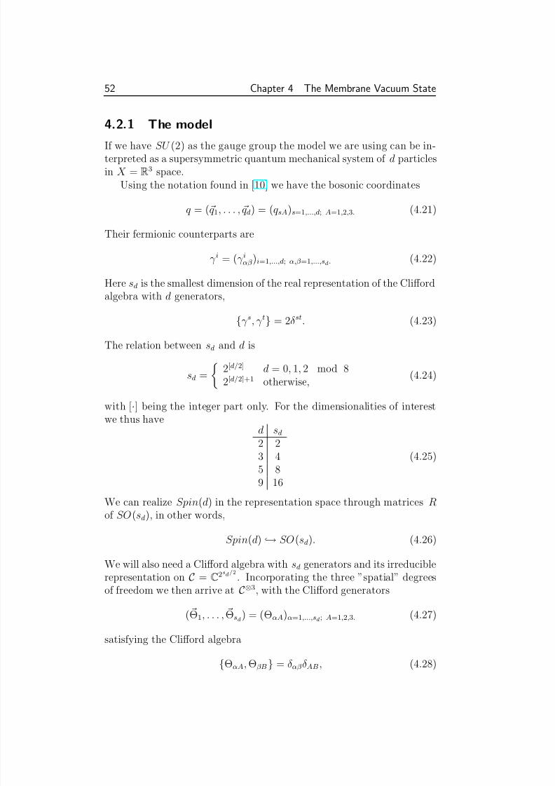
8/3/2019 Ronnie Jansson- The Membrane Vacuum State
http://slidepdf.com/reader/full/ronnie-jansson-the-membrane-vacuum-state 58/107
52 Chapter 4 The Membrane Vacuum State
4.2.1 The model
If we have SU (2) as the gauge group the model we are using can be in-terpreted as a supersymmetric quantum mechanical system of d particlesin X = R3 space.
Using the notation found in [10] we have the bosonic coordinates
q = (q1, . . . , qd) = (qsA)s=1,...,d; A=1,2,3. (4.21)
Their fermionic counterparts are
γ i = (γ iαβ )i=1,...,d; α,β =1,...,sd. (4.22)
Here sd is the smallest dimension of the real representation of the Cliffordalgebra with d generators,
γ s, γ t = 2δst. (4.23)
The relation between sd and d is
sd =
2[d/2] d = 0, 1, 2 mod 82[d/2]+1 otherwise,
(4.24)
with [·] being the integer part only. For the dimensionalities of interest
we thus haved sd
2 23 45 89 16
(4.25)
We can realize Spin(d) in the representation space through matrices Rof SO(sd), in other words,
Spin(d)
→SO(sd). (4.26)
We will also need a Clifford algebra with sd generators and its irreduciblerepresentation on C = C2sd/2. Incorporating the three ”spatial” degreesof freedom we then arrive at C⊗3, with the Clifford generators
( Θ1, . . . , Θsd) = (ΘαA)α=1,...,sd; A=1,2,3. (4.27)
satisfying the Clifford algebra
ΘαA, ΘβB = δαβ δAB, (4.28)
8/3/2019 Ronnie Jansson- The Membrane Vacuum State
http://slidepdf.com/reader/full/ronnie-jansson-the-membrane-vacuum-state 59/107
4.2 The SU (2) ground state theorem 53
which, if realized explicitly, should be done so with great care (we will
do this for the d = 3 case in the appendix). The Hilbert space is thus
H = L2(X, C⊗3) (4.29)
The supercharges that will act on the Hilbert space are
Qβ = Θα · (−iγ tαβ t +
1
2 qs × qtγ st
βα), (4.30)
where t are simply the partial derivatives w.r.t. qt and with α, β =1, . . . , s
dand s, t = 1, . . . , d, and where,
γ st =1
2(γ sγ t − γ tγ s). (4.31)
The supercharges transform as scalars under SU (2) gauge transforma-tions that are generated by
J AB = LAB + M AB ≡ −i(qsA∂ sB − qsB∂ sA) − i
2(ΘαAΘαB − ΘαBΘαA)
(4.32)and as spinors under the Spin(d) transformations generated by
J st = Lst + M st ≡ −i(qs · t − qt · s) − i
4 Θαγ st
αβ Θβ , (4.33)
To obtain the Hamiltonian of the system we need to calculate theanticommutation relations of the supercharges. Before we proceed withthis task a warning to sensitive souls and mathematicians is in order; thefollowing treatment will exhibit a certain laxness of index positioning.The inherent notation1 of the various quantities involved occasionallymake it highly undesirable to be too meticulous about those lesser things
in life. It should be strongly stressed, however, that clarity in the pre-sentation have not been sacrificed in favor of aesthetics (there are noaesthetic expressions in this chapter). If despite this someone would findthe following calculation hard to digest, please take a look at the originalwork [10] before voicing any complaints. It should also be noted that thecalculation is done for the case where d = 9.
Having thus dispensed with the amenities, we go right back to work.Anticommuting the supercharges immediately result in the following four
1We follow the original notation used in [10].
8/3/2019 Ronnie Jansson- The Membrane Vacuum State
http://slidepdf.com/reader/full/ronnie-jansson-the-membrane-vacuum-state 60/107
54 Chapter 4 The Membrane Vacuum State
terms,
Qα, Qβ =
Θγ · (−iγ tγα t), Θδ · (−iγ pδβ
p)
+
Θγ · 1
2 qs × qtγ st
αγ , Θδ · 1
2 q p × qqγ pq
βδ
+
Θγ · (−iγ tγα
t), Θδ · 1
2 q p × qqγ pq
βδ
+
Θγ · 1
2 qs × qtγ st
αγ , Θδ · (−iγ pδβ p)
= I + II + III + IV.
Starting with the first term, we have,
I = −γ tαγ γ pβδtA pBΘγA, ΘδB= −
γ (tγ s)
αβ tA pB δAB
= −1
2γ t, γ pαβ tA pB δAB = −δαβ
9s=1
2s , (4.34)
where we have simply used the Clifford algebras of ΘαA and γ s , respec-tively.
At this juncture we should also mention the symmetry/antisymmetry
of the γ -matrices, vital properties we will use consistently throughout ourcalculations,
γ (0), γ (1) symmetric
γ (2), γ (3) antisymmetric
γ (4), γ (5) symmetric
γ (6), γ (7) antisymmetric
γ (8), γ (9) symmetric
The second term becomes,
II =1
4γ st
αγ γ pqβδ ABC qsBqtC
DEF q pE qqF ΘγA, ΘδD
= −1
4
γ stγ pq
(αβ )
ABC qsBqtC EF
A q pE qqF
= −1
4
γ stγ pq
(αβ )
δBC EF qsBqtC q pE qqF
= −1
4
γ stpq
(αβ )
− 4δ[s[ p(γ
t]q])(αβ ) − 2δst
[ pq]δαβ
δBC
EF qsBqtC q pE qqF .
(4.35)
8/3/2019 Ronnie Jansson- The Membrane Vacuum State
http://slidepdf.com/reader/full/ronnie-jansson-the-membrane-vacuum-state 61/107
4.2 The SU (2) ground state theorem 55
Of the three terms above, only the last one survives. The first is zero
due to the antisymmetry in BCEF and symmetry of δ, the second due tosymmetry in αβ coupled with the antisymmetry of γ (2). To continue, wenow have
. . . = −1
4δαβ δ
BC EF (qsBqtC qtE qsF − qsBqtC qsE qtF )
= δαβ 1
2(ABC qsBqtC )
2 = δαβ
s<t
(qs × qt)2. (4.36)
To proceed with III and IV we need to calculate two terms containingderivatives. Term III is
− i2
Θ A
γ Θ Dδ γ tγα γ pq
βδtADEF qE
p q F q + Θ D
δ Θ Aγ γ pq
βδ γ tγαDEF qE
p q F q
At
= − i
2
Θ A
γ Θ Dδ γ tγα γ pq
βδ DEF
δtp δAE q F
q + δtq δAF q E p + q E
p q F q
At
+ Θ D
δ Θ Aγ γ pq
βδ γ tγαDEF qE
p q F q
At
. (4.37)
In the next step we will use the simple relation
AB =1
2[A, B] +
1
2A, B. (4.38)
Contracting indices and using the antisymmetry of DEF we obtain,
III = − i
2
Θ
[E (γ Θ
D]δ) γ tγαγ tq
βδ DEF qF
q
+ Θ[F (γ Θ
D]δ) γ tγα γ tq
βδ DEF qE
p
+ Θ[A(γ Θ
D]δ) γ tγαγ pq
βδ DEF qE
p q F q
At
+1
2γ tδαγ pq
βδ DEF qE
p q F q
Dt
+ Θ Dδ Θ A
γ γ pqβδ γ tγα DEF q
E p q F
q A
t
, (4.39)
and a very similar result for term IV . Taking the non-Θ-terms of III
and IV together and renaming dummy indices, we get
− i
4
γ pδβ γ st
αδ + γ pδαγ stβδ
ABC q
Bs q C
t A
p . (4.40)
By manipulating the Dirac matrices according to,
γ pδβ γ stαδ + γ pδαγ st
βδ =
γ stγ p − γ pγ st
αβ
=1
2
γ sγ tγ p − γ tγ sγ p − γ pγ sγ t + γ pγ tγ s
αβ
= 2
δ ptγ s − δspγ t
αβ
, (4.41)
8/3/2019 Ronnie Jansson- The Membrane Vacuum State
http://slidepdf.com/reader/full/ronnie-jansson-the-membrane-vacuum-state 62/107
56 Chapter 4 The Membrane Vacuum State
and inserting this result into (4.40) we get,
− i
2γ tαβ q
At ABC
q B
s C
s − q C s
Bs
. (4.42)
Saving this for later and instead collecting the remaining terms in III and IV containing derivatives we are faced with these two creatures,
− i
2Θ A
γ Θ Dδ
γ st
αγ γ pδβ + γ stβγ γ pδα
ABC q
Bs q C
t pD (4.43)
− i
2Θ
[D(δ Θ
A]γ )
γ st
αγ γ pδβ + γ stβγ γ pδα
ABC q
Bs q C
t pD. (4.44)
Again using (4.38) and cancelling some terms, we end up with
− i
4
γ st
αδγ pδβ + γ stβδ γ pδα
ABC q
Bs q C
t A
p
= − i
2
γ sαβ ABC q
Bs q C
t A
t − γ tαβ ABC qB
s q C t
As
= − i
2γ tαβ q
At ABC
q B
s C
s − q C s
Bs
. (4.45)
The only terms in III and IV we have not yet dealt with are thosewithout derivatives, namely,
−iΘ
[B(δ Θ
A]γ ) γ sδβ γ st
αγ + γ sδαγ stβγ ABC q
C t . (4.46)
Since it is not matrix multiplication of the Dirac matrices we are forcedto Fierz the expression. We immediately note that due to symmetryrequirements and the fact that γ (5≤n≤9) is already included in γ (0≤n≤4),the only terms that remain are those for n = 0 and n = 4,
γ s(α(γ γ stβ )δ) = a δαβ γ tγδ + b γ tαβ δγδ
+ c γ s1...s4αβ γ s1...s4t
γδ + d γ s1...s4tαβ γ s1...s4
γδ . (4.47)
By using the totally antisymmetric tensor on the last term we can trans-form it into the c-term. We thus exclude the last term, and then contract
both sides of the equation with (γ t
)βγ
. This yields,
L.H.S =1
4
γ tβγ
γ sαγ γ stβδ + γ sαδγ st
βγ + γ sβγ γ stαδ + γ sβδ γ st
αγ
=
1
4
γ sγ tγ st
αδ
− γ sγ tγ st
αδ
= 0. (4.48)
The contracted right-hand side of (4.47) becomes,
R.H.S = a
γ tγ t
αδ+ b
γ tγ t
αδ
+ 5cγ s1...s4αβ γ s1...s4
γδ
= 9aδαδ + 9bδαδ + 5(−6)7(−8)9cδαδ. (4.49)
8/3/2019 Ronnie Jansson- The Membrane Vacuum State
http://slidepdf.com/reader/full/ronnie-jansson-the-membrane-vacuum-state 63/107
4.2 The SU (2) ground state theorem 57
Thus we have the relation,
a + b + 1680c = 0. (4.50)
To proceed, we now contract (4.47) with δαβ , giving us
L.H.S =1
4
γ sγ st + γ sγ st + γ sγ st + γ sγ st
= 8γ t, (4.51)
and
R.H.S = 16aγ t. (4.52)
Instead contracting with δγδ produces a similar relation for the b-term,except for an additional minus sign hailing from the antisymmetry of γ st.We thus have the following:
a =1
2, b = −1
2. (4.53)
Putting this result into (4.50) gives us c = 0, and we can write down theFierzed equation,
γ sδβ γ stαγ + γ sδαγ st
βγ = δαβ γ tγδ
−γ tαβ δγδ , (4.54)
which, inserted into (4.46), becomes
−iδαβ qC
t ABC Θ[B(δ Θ
A]γ )γ tγδ + iγ tαβ q
C t ABC Θ
[Bγ ΘA]
γ . (4.55)
This we can rewrite as
iδαβ qs ·
Θγ × Θδ
γ sγδ − 1
2iγ tαβ q
At
ΘB
γ ΘC γ − ΘC
γ ΘBγ
. (4.56)
We have now finished the calculation of the anticommutation relations
of the supercharges. Gathering the results we have,
Qα, Qβ = δαβ H + γ tαβ qtAABC J BC , (4.57)
with the Hamiltonian being
H = −9
s=1
2s +
s<t
( qs × qt)2 + i qs · ( Θα × Θβ )γ sαβ , (4.58)
which furthermore commutes with J AB and J st.
8/3/2019 Ronnie Jansson- The Membrane Vacuum State
http://slidepdf.com/reader/full/ronnie-jansson-the-membrane-vacuum-state 64/107
58 Chapter 4 The Membrane Vacuum State
4.2.2 The theorem
The question we want answered is now whether there exist a normalizablestate Ψ ∈ H, that is a singlet with respect to SU (2) and Spin(d), andfulfills
Hψ = 0 (4.59)
i.e., have zero energy. An equivalent, but much easier route is to look forthe zero-modes,
Qβ ψ = 0, β = 1, . . . , sd. (4.60)
It should also be noted that the requirement of Spin(d) invariance is nottrivial. The full argument is presented in [61].
Introducing the variable r > 0, and the unit vectors e and E s obeying
e 2 = 1,
s
E 2s = 1, (4.61)
the bosonic potential
s<t(qs × qt)2 will vanish on the manifold
qs = reE s. (4.62)
The dimension of this manifold is
1 + 2 + (d−
1) . (4.63)
r e E s
Furthermore, we can express points in a conical neighborhood of themanifold by making use of tubular coordinates,
qs = reE s + r−1/2ys, (4.64)
where r−1/2 have been added not out of necessity but to simplify for uslater on. The transversal coordinates ys obey
ys · e = 0s, ysE s = 0. (4.65)
We also need to remark that qs is invariant under the antipode map,
(e, E, y) −→ (−e, −E, y). (4.66)
Therefore we will look for, and include, only those states that are evenunder this transformation.
We are now ready to present the theorem describing the possibleground state. The formulation of the theorem is taken verbatim from [10].
8/3/2019 Ronnie Jansson- The Membrane Vacuum State
http://slidepdf.com/reader/full/ronnie-jansson-the-membrane-vacuum-state 65/107
4.2 The SU (2) ground state theorem 59
Theorem 4.1 Consider the equations Qβ ψ = 0 for a formal power series
solution near r = ∞ of the form
ψ = r−κ∞
k=0
r−3
2kψk, (4.67)
where : ψk = ψk(e, E, y) is square-integrable w.r.t. de dE dy;ψk is SU(2) × Spin(d) invariant ;ψ0 = 0.
Then, up to linear combinations,
• d = 9: The solution is unique, and κ = 6;
• d = 5: There are three solutions with κ = −1 and one with κ = 3;
• d = 3: There are two solutions with κ = 0;
• d = 2: There are no solutions.
All solutions are even under the antipode map (4.66),
ψk(e, E, y) = ψk(−e, −E, y), (4.68)
except for the state d = 5, κ = 3, which is odd, and thus not a viableground state.
When we check whether a possible ground state is square-integrable ornot we use the integration measure
dq = dr · r2de · rd−1dE · r1
2·2(d−1)dy = r2dr de dE dy (4.69)
Thus, for ψ to be square integrable (at infinity) ∞dr r2(r−κ)2 < ∞ (4.70)
must hold. This is fulfilled if κ > 3/2. Hence we can immediately removethe solutions for d = 3, and d = 5 with κ = −1. As was already pointedout, the solution d = 5 with κ = 3 is odd under the antipode map (4.66)and thus cannot be a ground state. This makes d = 9 the sole survivor,and as this case corresponds to the eleven-dimensional supermembrane,it makes us warm all over.

8/3/2019 Ronnie Jansson- The Membrane Vacuum State
http://slidepdf.com/reader/full/ronnie-jansson-the-membrane-vacuum-state 66/107
60 Chapter 4 The Membrane Vacuum State
4.3 The Proof
To prove theorem 4.1 we will expand the supercharges in power seriesand match these with the power series of the conjectured wave functions(4.67). This will yield n → ∞ equations, where n = 0 correspondsto Q0
β ψ0 = 0. We then proceed by solving this initial case, and find asolution that is not necessarily SU (2)×Spin(d) invariant. Next we checkwhat states are singlets of SU (2) × Spin(d) and proceed to check thatthe states are even under the antipode map (4.66). We then continueby investigating the equations for n > 0 and then finally determine thedifferent values of κ for the various values of d.
4.3.1 The d = 2 case
The fact that no ground state can exist for d = 2 can easily be derivedwithout going through the full proof. By examining J st and showing thatno state J 12 satisfying
J 12ψ = 0 (4.71)
exists, it follows that no Spin(d) invariant ground state is possible ford = 2. We start by constructing M 12. For d = 2 we have sd = 2 and canuse the standard Pauli matrices, choosing
γ
1
= σ
1
, γ
2
= σ
3
. (4.72)Thus yielding,
γ 12 =
0 −11 0
. (4.73)
For M 12 we now get,
M 12 = − i
4ΘαAγ 12αβ ΘβA =
i
4(Θ1AΘ2A − Θ2AΘ1A)
=i
2Θ1AΘ2A, (4.74)
where we sum over A = 1, 2, 3. We will also need the six Clifford gener-ators ΘαA. We construct these according to2,
Θα1 =1√
2(σα ⊗ 1 2 ⊗ σ3)
Θα2 =1√
2(σ3 ⊗ σα ⊗ 1 2)
Θα3 =1√
2( 1 2 ⊗ σ3 ⊗ σα) .
2More on this scheme can be found in appendix C.
8/3/2019 Ronnie Jansson- The Membrane Vacuum State
http://slidepdf.com/reader/full/ronnie-jansson-the-membrane-vacuum-state 67/107
4.3 The Proof 61
Explicitly using these 8
×8 matrices and forming (M 12)2 we obtain a
diagonal matrix whose elements are the squared eigenvalues of M 12. Theextracted eigenvalues are 1/4 and 3/4. The final observation that need tobe done is that L12 has the spectrum Z, thus making any state fulfillingJ 12ψ = 0 impossible.
4.3.2 Power series expansion of Qβ
To make a power series expansion of the supercharges Qβ we first needto obtain the derivative
∂
∂qtA
= r1/2(δst
−E sE t)(δAB
−eAeB)
∂
∂ysB
+r−1
eAE t
r
∂
∂r+
1
2ysB
∂
∂ysB
+ ieBE tLBA + ieAE sLst
+O(r−5/2). (4.75)
To show this we need to calculate the partial derivatives contained in
∂
∂qtA=
∂r
∂qtA
∂
∂r+
∂eB
∂qtA
∂
∂eB+
∂E s∂qtA
∂
∂E s+
∂ysB
∂qtA
∂
∂ysB. (4.76)
Fromqs = reE s + r−1/2ys (4.77)
we get
dqtA =
eAE t − 1
2r−3/2ytA
dr + rE tdeA + reAdE t + r−1/2dytA. (4.78)
We then use the coordinate relations (4.65) and (4.61) to obtain
eAdytA + ytAdeA = 0 (4.79)
E tdytA + ytAdE t = 0 (4.80)
eAdeA = 0 (4.81)
E tdE t = 0. (4.82)
Using these relations we derive the following contractions of (4.78),
eAE tdqtA = dr, (4.83)
(δAB − eAeB)E tdqtA = rdeB − r−1/2ytBdE t, (4.84)
eA(δst − E sE t)dqtA = rdE s − r−1/2ysAdeA, (4.85)
(δAB − eAeB)(δst − E sE t)dqtA = −1
2r−1/2(dysB + eBysAdeA
+E sytBdE t). (4.86)
8/3/2019 Ronnie Jansson- The Membrane Vacuum State
http://slidepdf.com/reader/full/ronnie-jansson-the-membrane-vacuum-state 68/107
62 Chapter 4 The Membrane Vacuum State
To proceed we introduce two matrices m and M :
mAB = δAB − r−3ytAytB, (4.87)
M st = δst − r−3ysAytA. (4.88)
These matrices are then used to express the differentials deB and dE s:
deB = (m−1)BC (r−1(δCA − eC eA)E t + r−5/2ytC eA)dqtA, (4.89)
dE s = (M −1)su(r−1(δut − E uE t)eA + r−5/2ysAE t)dqtA. (4.90)
The validity of the above statements is most easily checked by multiplyingequation (4.84) with both m and M , and then inserting the expressions(4.87)-(4.90) and checking that the equality still holds. By expanding mand M we rewrite the differentials as
deB = (r−1(δBA − eBeA)E t + O(r−5/2))dqtA, (4.91)
dE s = (r−1(δst − E sE t)eA + O(r−5/2))dqtA. (4.92)
We can now write down the four differentials
dr = eAE tdqtA, (4.93)deB = (r−1(δBA − eBeA)E t + O(r−5/2))dqtA, (4.94)
dE s = (r−1(δst − E sE t)eA + O(r−5/2))dqtA, (4.95)
dysB = [r1/2(δBA − eBeA)(δst − E sE t)
+1
2r−1eAE tysB]dqtA − eBysAdeA − E sytBdE t, (4.96)
which makes it a simple matter to express the partial derivatives in (4.76)as:
∂ ∂qtA
= r1/2(δst − E sE t)(δAB − eAeB) ∂ ∂ysB
+r−1[eAE t(r det r +1
2ysB
∂
∂ysB)]
+r−1(δAC − eAeC )E t(δCB∂
∂eB− eBysC
∂
∂ysB)
+r−1(δut − E uE t)eA(δus∂
∂E s− E syuB
∂
∂ysB)
+O(r−5/2), (4.97)
8/3/2019 Ronnie Jansson- The Membrane Vacuum State
http://slidepdf.com/reader/full/ronnie-jansson-the-membrane-vacuum-state 69/107
4.3 The Proof 63
where the last term does not contain any derivatives with respect to r.
By inserting this into iLBA we get
iLBA = qsB∂
∂qsA− qsA
∂
∂qsB
= [(δAC − eAeC )ysB − (δBC − eBeC )ysA]∂
∂ysB
+eB(δAC ∂
∂eC − eC ysA
∂
∂ysC )
−eA(δBC ∂
∂eC − eC ysB
∂
∂ysC ). (4.98)
This allows us to write down
ir−1eBE tLBA = r−1(δAC − eAeC )E t(δCB∂
∂eB− eBysC
∂
∂ysB), (4.99)
and in analogy with this, also
ir−1eAE sLst = r−1(δut − E uE t)eA(δus∂
∂E s− E syuB
∂
∂ysB), (4.100)
which, together with (4.97) forms our sought-after derivative (4.75).We are now armed and ready to expand Qβ ,
Qβ = Θα · (−iγ tαβ t +
1
2qs × qtγ st
βα)
= −iΘαAγ tαβ r1/2(δst − E sE t)(δAB − eAeB) ∂
∂ysB
−iΘαAγ tαβ r−1(eAE tr(
∂
∂t+
1
2ysB
∂
∂ysB))
+ΘαAγ tαβ r−1(eBE tLBA + eAE sLst)
+ Θα · r1/2(e × yt)E sγ stβα
+1
2 Θα · r−1(ys × yt)γ st
βα + O(r−5/2). (4.101)
Next we identify the r-independent operators which we will match with
orders of r−3n
2
,
Q0β = −iΘαAγ tαβ (δst − E sE t)(δAB − eAeB)
∂
∂ysB
+ Θα · (e × yt)E sγ stβα, (4.102)
Q1β = −i( Θα · e)γ tαβ E t, (4.103)
Q1β = ΘαAγ tαβ (eBE tLBA + eAE sLst − i
2eAE tysB
∂
∂ysB)
+1
2 Θα(ys × yt)γ st
βα. (4.104)
8/3/2019 Ronnie Jansson- The Membrane Vacuum State
http://slidepdf.com/reader/full/ronnie-jansson-the-membrane-vacuum-state 70/107
64 Chapter 4 The Membrane Vacuum State
Higher order terms will not be needed explicitly. We now pair these
operators with powers of r and get the power series expansion of Qβ :
Qβ = r1/2Q0β + r−1(Q1
β r∂
∂r+ Q1
β ) + r−5/2Q2β + . . . . (4.105)
Q0β Q1
β Q2β
Now, before we write down the equation Qβ ψ = 0 in all its glory we needto introduce an alternative notation for ψ (cf. previous definition (4.67)),
ψ =∞
n
ψn. (4.106)
By noting the powers of r in Qnβ and ψn,
Qmβ ∼ r
1
2−3m
2 , (4.107)
ψn ∼ r−(κ+ 3n2), (4.108)
we find the m-independent quantity,
Qmβ ψn−m ∼ r−κ−3n
2+ 1
2 . (4.109)
Thus we can finally write down the equation Qβ ψ = 0,
Q0β ψn + (−(κ + 32(n − 1))Q1β + Q1β )ψn−1 + Q2β ψn−2 + . . . + Qnβ ψ0 = 0,
(4.110)
where n = 0, 1, . . ..
4.3.3 The equation at n = 0
For n = 0 the equation (4.110) is simply
Q0β ψ0 = 0. (4.111)
This equation admits precisely the solutionsψ0(e, E, y) = e−
P
s y2s/2 |F (E, e) . (4.112)
This solution, however, is not necessarily SU (2)×Spin(d) invariant, andimposing this condition is something we will do later. To describe thefermionic states |F (E, e) we first introduce the two complex vectors n±,satisfying
n+ · n− = 1 (4.113)
e × n± = in±, (4.114)
8/3/2019 Ronnie Jansson- The Membrane Vacuum State
http://slidepdf.com/reader/full/ronnie-jansson-the-membrane-vacuum-state 71/107
4.3 The Proof 65
and thus also
n± · n± = 0 (4.115)
n+ × n− = −ie. (4.116)
Explicit derivations of n± are done in appendix C. We now introducethe vectors u, v ∈ Rsd and Θ(v) = Θαvα, allowing us to construct thefermionic operators
Θ(v) · n±. (4.117)
These operators satisfy the anticommutation relations,
Θ(u) · n+,
Θ(v) · n− = uαΘαAn
A
+, vβ ΘβB n
B
−= uαvβ n
A+nB
−δαβ δAB
= uαvα(n+ · n−)
= uαvα. (4.118)
By the same procedure and using (4.115) we also obtain
Θ(u) · n±, Θ(v) · n± = 0. (4.119)
Next, we want to calculate Q0α, Q0
β , and as we have already done thiscalculation for the complete supercharges we only give the results,
Q0α, Q0
β = δαβ H 0 + γ tαβ E tABC M ABeC , (4.120)
where the Hamiltonian is,
H 0 =
−(δst − E sE t)(δAB − eAeB)
∂
∂ysA
∂
∂ytB+
s
y2s
+i E sγ sαβ e · ( Θα × Θβ ) = H 0B + H 0F . (4.121)
What we now aim to do is prove that the fermionic states |F (E, e) have
to satisfy
Θ(v) · n± |F (E, e) = 0, when E sγ sv = ±v. (4.122)
In other words, we want to show that equation (4.111) implies (4.122).To accomplish this we begin by contracting equation (4.120) with δαβ
and then with γ tαβ E t we see that equation (4.111) in fact correspond to,
H 0ψ0 = 0 (4.123)
ABC M ABeC ψ0 = 0. (4.124)
8/3/2019 Ronnie Jansson- The Membrane Vacuum State
http://slidepdf.com/reader/full/ronnie-jansson-the-membrane-vacuum-state 72/107
66 Chapter 4 The Membrane Vacuum State
The next step is to show that these two equations are satisfied if and only
if (4.122) holds. We begin by noting that the bosonic Hamiltonian, H 0B,is a harmonic oscillator with 2(d − 1) degrees of freedom. Moreover, itcarries the energy 2(d− 1) and as a ground state have the wave function,
ϕ0B = e−
P
s y2s2 . (4.125)
To investigate the fermionic part of the Hamiltonian, we write
H 0F = iE sγ sαβ e · ( Θα × Θβ ) = −E sγ sαβ (n+ × n−)( Θα × Θβ )
= E sγ sαβ Θα · (n+ × n−) × Θβ = −E sγ sαβ
Θα Θβ × (n+ × n−)
= −E sγ sαβ (( Θα · n+)( Θβ · n−) − ( Θα · n−)( Θβ · n+)). (4.126)
To proceed further we decompose E sγ sαβ into projection operators,
E sγ sαβ = P + − P −, (4.127)
where the sd × sd matrices have half of their diagonal elements set tounity,
P + = diag(1, . . . , 1, 0, . . . , 0), P − = diag(0, . . . , 0, 1, . . . , 1). (4.128)
To continue we now get,
(4.126) = −P +αβ ( Θα · n+)( Θβ · n−) + P +αβ (
Θα · n−)( Θβ · n+)
+P −αβ ( Θα · n+)( Θβ · n−) − P −αβ (
Θα · n−)( Θβ · n+)
= −P +αα + P +αβ ( Θα · n−)( Θβ · n+) + P +αβ (
Θα · n−)( Θβ · n+)
+P −αβ ( Θα · n+)( Θβ · n−) − P −αα + P −αβ (
Θα · n+)( Θβ · n−)
= −sd + 2P +αβ ( Θα · n−)( Θβ · n+) + 2P −αβ (
Θα · n+)( Θβ · n−)
(4.129)
where we used the Clifford algebra and the structure of the projectionoperators. The attentive reader immediately note from (4.25) that
sd = 2(d − 1). (4.130)
Thus will the first term in H 0F cancel the energy contribution from thebosonic part of the Hamiltonian. Furthermore we see that the remainingterms in H 0F kill the state |F (E, e) if the condition (4.122) holds. Inother words, H 0ψ0 = 0, and we are left to show that (4.124) annihilates
8/3/2019 Ronnie Jansson- The Membrane Vacuum State
http://slidepdf.com/reader/full/ronnie-jansson-the-membrane-vacuum-state 73/107
4.3 The Proof 67
|F (E, e)
,
ABC M ABeC ψ0 = − i
2ABC (ΘαAΘαB − ΘαBΘαA)eC
= −iABC ΘαAΘαBeC
= −ie · ( Θα × Θα)
= (n+ × n−) · ( Θα × Θα)
= ( Θα · n+)( Θα · n−) − ( Θα · n−)( Θα · n+), (4.131)
where we in the second to last equality used the same reasoning as in theprevious calculation for H 0F . Now using the structure of the projection
operators, we get
. . . = P +αβ ( Θα · n+)( Θα · n−) + P −αβ (
Θα · n+)( Θα · n−)
−P +αβ ( Θα · n−)( Θα · n+) − P +αβ (
Θα · n−)( Θα · n+)
= 2P −αβ ( Θα · n+)( Θα · n−) − 2P +αβ (
Θα · n−)( Θα · n+), (4.132)
where we in the last equality used the Clifford algebra. It is immediatelyapparent that this expression annihilates |F (E, e).
To recapitulate, we have thus derived the form (4.112) of the solutionsto the equation Q0
β ψ0 = 0, and specifically shown the conditions (4.122)
the state |F (E, e) must obey.
4.3.4 Extracting allowed states
The remaining parts of the proof will not be given in full detail. Insteadthe remaining steps will be given a slightly more brief explanation. Thereader who wish to delve into the details is referred to [10].
Having obtained and described ψ0 satisfying Q0β ψ0 = 0, the next
step is to extract the states which are SU (2) × Spin(d) invariant. Aswe mentioned in section 4.2.1, we have Spin(d) → SO(sd). LettingR
∈SO(sd) and U
∈SU (2) there is a natural representation of SU (2)
×Spin(d) on the Hilbert space H = L2(X, C⊗3). SU (2) × Spin(d) actnaturally on X through the representation SO(3) × SO(d). In the caseof C⊗3 we have the representation R of Spin(sd) R, satisfying
R(R)∗ΘαAR(R) = Rαβ ΘβA, (4.133)
where R = R(R) is its above mentioned SO(sd) representation. Using(4.26) together with the fact that
SO(sd) = Spin(sd)/(Z )2, (4.134)
8/3/2019 Ronnie Jansson- The Membrane Vacuum State
http://slidepdf.com/reader/full/ronnie-jansson-the-membrane-vacuum-state 74/107
68 Chapter 4 The Membrane Vacuum State
we obtain
Spin(d) → Spin(sd). (4.135)
In other words, we have shown that R is a representation of Spin(d).Similarly, we have the representation U of SU (2) U on C⊗3,
U (U )∗ΘαA U (U ) = U ABΘαB. (4.136)
Now, the SU (2) × Spin(d) invariant states are those satisfying,
U (U ) |F (E, e) = |F (E, Ue) (4.137)
R(R) |F (E, e) = |F (RE, e) , (4.138)
where (U, R) ∈ SU (2) × Spin(d). The above states are furthermore inbijective correspondence to the states invariant under (U, R) ∈ U (1) ×Spin(d − 1). In other words states satisfying
U (U ) |F (E, e) = |F (E, e) (4.139)
R(R) |F (E, e) = |F (E, e) , (4.140)
for some arbitrary but fixed (E, e), and where Ue = e and RE = E .
After replacing ΘαA with operators Θα·e which leave the space (4.122)invariant, it turns out that this representation decomposes into
C= 2(sd/2)−1+ ⊕ 2(sd/2)−1− . (4.141)
The embedding (4.135) and the branching of the representation dependon our choice of Dirac matrices. After a certain choice (see [10] for details)the representation of Spin(d) branches into,
C =
(44 ⊕ 84) ⊕ 128 , d = 9(5 ⊕ 1 ⊕ 1 ⊕ 1) ⊕ (4 ⊕ 4) , d = 52 ⊕ (1 ⊕ 1) , d = 3.
(4.142)
We will get additional branching for Spin(d − 1) → Spin(d),
C = (1 ⊕ 8v ⊕ 35v) ⊕ (28 ⊕ 56v) ⊕ (8s ⊕ 8c ⊕ 56s ⊕ 56c) , d − 1 = 81 ⊕ 1 ⊕ 1 ⊕ (1 ⊕ 4) ⊕ (2+ ⊕ 2−) ⊕ (2+ ⊕ 2−) , d − 1 = 4
(11 ⊕ 1−1) ⊕ 10 ⊕ 10 , d − 1 = 2.(4.143)
After some further analysis we find the invariant states of interest,and the Spin(d) representation to which they are associated,
d = 9 : 44
d = 5 : 1, 1, 1, 5
d = 3 : 1, 1
8/3/2019 Ronnie Jansson- The Membrane Vacuum State
http://slidepdf.com/reader/full/ronnie-jansson-the-membrane-vacuum-state 75/107
4.4 A numerical method 69
The next step in the proof is to check that the states are even under
the antipode map (4.66). Doing so excludes only one of the states ford = 5. After that we need to analyze the equations (4.110) for n ≥ 1.Doing this, we obtain relations needed for the final step, determining κ.Accomplishing this task and obtaining the values of κ presented in theformulation of the theorem then concludes the proof.
4.4 A numerical method
An alternate approach to characterize the membrane vacuum state hasrecently been proposed by Wosiek [63]. The main idea is to solve prob-lems in supersymmetric Yang-Mills quantum mechanics in various di-mensions by way of an algebraic program. Wosiek has managed to con-firm many old results and also obtain some new ones, especially for thecase of D = 4 super Yang-Mills theory. The, for our purposes, moreinteresting case of D = 10 (which corresponds the supermembrane ineleven-dimensional spacetime) was investigated further in [64] with someadditional results derived in [65].
Supersymmetric Yang-Mills quantum mechanics has many features incommon with more advanced field theories and as such provides a nice
”theoretician’s laboratory” to study supersymmetry in various guises.Beside the importance of D = 10 as a model of the supermembrane andits connection to M-theory, this technique have been applied to SU (2)invariant Wess-Zumino quantum mechanics and various dimensions of supersymmetric Yang-Mills quantum mechanics.
The main theme of Wosiek’s approach is to implement the Hamilto-nian formulation of quantum mechanics into the logical structure of acomputer. Vectors in some Hilbert space are represented by lists withdynamically varying size. Quantum operators are then just functions of these lists. The main computational problem is to limit the size of theHilbert space which of course limits the number of degrees of freedomthat can be allowed. This introduced cut-off, however, is easily mon-itored and by increasing the cut-off one can find convergent results of eigenvalues and thus obtain trustworthy results.
By using the discrete eigenbasis of the occupation number a†a wehave
|n, |n =1√n!
(a†)n |0 . (4.144)
Furthermore, we can write the bosonic coordinate and momentum oper-
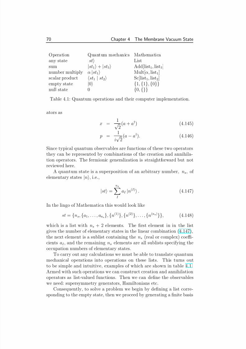
8/3/2019 Ronnie Jansson- The Membrane Vacuum State
http://slidepdf.com/reader/full/ronnie-jansson-the-membrane-vacuum-state 76/107
70 Chapter 4 The Membrane Vacuum State
Operation Quantum mechanics Mathematica
any state |st Listsum |st1 + |st2 Add[list1, list2]number multiply α |st1 Mult[α, list1]scalar product st1 | st2 Sc[list1, list2]empty state |0 1, 1, 0null state 0 0, Table 4.1: Quantum operations and their computer implementation.
ators as
x = 1√2
(a + a†) (4.145)
p =1
i√
2(a − a†). (4.146)
Since typical quantum observables are functions of these two operatorsthey can be represented by combinations of the creation and annihila-tion operators. The fermionic generalization is straightforward but notreviewed here.
A quantum state is a superposition of an arbitrary number, ns, of elementary states |n, i.e.,
|st =nsI
aI |n(I ) . (4.147)
In the lingo of Mathematica this would look like
st = ns, a1, . . . , ans, n(1), n(2), . . . , n(ns), (4.148)
which is a list with ns + 2 elements. The first element in in the listgives the number of elementary states in the linear combination (4.147),the next element is a sublist containing the ns (real or complex) coeffi-
cients aI , and the remaining ns elements are all sublists specifying theoccupation numbers of elementary states.To carry out any calculations we must be able to translate quantum
mechanical operations into operations on these lists. This turns outto be simple and intuitive, examples of which are shown in table 4.1.Armed with such operations we can construct creation and annihilationoperators as list-valued functions. Then we can define the observableswe need: supersymmetry generators, Hamiltonians etc.
Consequently, to solve a problem we begin by defining a list corre-sponding to the empty state, then we proceed by generating a finite basis
8/3/2019 Ronnie Jansson- The Membrane Vacuum State
http://slidepdf.com/reader/full/ronnie-jansson-the-membrane-vacuum-state 77/107
4.4 A numerical method 71
of N cut-off vectors and calculate the quantum observables we need. Next,
we let the computer execute the program, and if it is the spectrum of the system we are interested in, we simply extract the energy eigenvaluesfrom the Hamiltonian matrix.
The results obtained using this method have been substantial in thecase of D = 4, which have been fully solved. Specifically, the spectrumhave been obtained with its pattern of discrete and continuous states.The cut-off can be chosen high enough for the restrictions on the Hilbertspace to become irrelevant.
In D = 10 problems arise. The number of states and hence the com-putational time increase rapidly as we go up in dimensions. No trustwor-thy results have thus been obtained for the full D = 10 case. However,various schemes have been suggested and developed to overcome thisproblem. One obvious choice is to exclude the fermionic part of the cal-culation, greatly reducing the number of states involved. By doing thisthe calculation gets manageable and the lower levels of the spectrum canbe found. In the end, the full supersymmetric case is the only case of real interest (at least for our purposes) and judging by the progress madeby Wosiek in each consecutive published paper in less than two years op-timism seem to be in order. In addition, as computational power is agreatly limiting factor and reading that Wosiek is using a common work-station for his research one cannot help but wonder what results could
be obtained if he was given some time on a supercomputer.
8/3/2019 Ronnie Jansson- The Membrane Vacuum State
http://slidepdf.com/reader/full/ronnie-jansson-the-membrane-vacuum-state 78/107
72 Chapter 4 The Membrane Vacuum State
8/3/2019 Ronnie Jansson- The Membrane Vacuum State
http://slidepdf.com/reader/full/ronnie-jansson-the-membrane-vacuum-state 79/107
5
ConclusionsIn our goal to examine the membrane vacuum state, we started out bytreating the bosonic membrane and investigating its symmetries, dy-namics and quantization properties. After introducing supersymmetrywe derived the allowed p-branes and target space dimensionalities. Weinvestigated further the properties of the super p-brane action in theHamiltonian formulation and the lightcone gauge. The APD algebraand its connection with matrix theory was analyzed and worked through
with the example of toroidal membranes.Dimensional reduction of super Yang-Mills theory was performed andits connection to the description of N D0-branes was commented upon.
The spectrum of both bosonic and supersymmetric membranes wasput under close scrutiny and discussed in detail.
In the main chapter we made a brief summary of the research con-ducted so far in the search for the membrane vacuum state. We then pro-ceeded by investigating a supersymmetric two-dimensional model with anx2y2 potential and conclusively proved that no normalizable ground statecould exist, a question that remained unsolved for more than a decadeand was resolved only recently. We then turned to the central theme of
this thesis and treated the SU (2) × Spin(d) invariant supersymmetricmatrix model. In essence, using the first order supercharges Qβ and firstorder perturbation theory to obtain a solution to
Qβ ψ = 0, (5.1)
where β counts the number of supercharges. We then formulated thetheorem regarding the existence and asymptotic form of the possibleground states. For the allowed dimensions d = 2, 3, 5, 9 of the modelthe power law decay of the zero-energy solutions was obtained, with thefollowing result:
73

8/3/2019 Ronnie Jansson- The Membrane Vacuum State
http://slidepdf.com/reader/full/ronnie-jansson-the-membrane-vacuum-state 80/107
74 Chapter 5 Conclusions
•d = 9 : A unique, normalizable solution.
• d = 5 : Three solutions, none of which were normalizable.
• d = 3 : Two solutions, none of which were normalizable.
• d = 2 : No solutions.
The form of the asymptotic (near r = ∞) solution we found for the caseof d = 9 was,
ψ =∞
k=0
r−3
2k−6ψk, (5.2)
where ψk is SU (2) × Spin(d) invariant and square-integrable on surfaceswhere r is constant.
The dimensionality d of the model is related to the dimensionalityD of the spacetime where the supermembrane propagates according toD = d + 2. Thus the only normalizable solution correspond to the reg-ulated supermembrane theory in eleven dimensions. Hence the prospectof finding the true membrane vacuum state remain very much a possi-bility. While work will likely continue on generalizing the SU (2) modelto arbitrary N , meanwhile exciting results could very well be obtainedfrom the computational methods of Wosiek, presented in chapter 4.
Having thus briefly summarized what has been done in this thesis,some remarks about what has not been done would be in order. Inaddition, some things which should have been done in greater detailis worthy of comment. The most obvious item would be the slightlyabbreviated proof of the main theorem, a proof which certainly deservesto be concluded with the same degree of attention it was begun with.
Another area I would have wished to pursued further is the compu-tational methods of super Yang-Mills quantum mechanics. The methodis still in its infancy and I believe it holds great promise in supplying, if nothing else, at least results to serve as a guide for the purely analytical
efforts being conducted.Membrane theory is a surprisingly large field, and though havingspent a year within its boundaries there are many aspects that by neces-sity have been left unstudied. For instance the ”spinning membrane” andsuperembeddings could be argued to have a place in a thesis like this.As would the full proof of the continuity of the quantum supermembranespectrum.
In the case of the SU (2) matrix model we could have examined fur-ther the requirement that the groundstate be Spin(d) invariant, or morethoroughly investigated the work done regarding SU (N > 2) invariant
8/3/2019 Ronnie Jansson- The Membrane Vacuum State
http://slidepdf.com/reader/full/ronnie-jansson-the-membrane-vacuum-state 81/107
Conclusions 75
generalizations of the model. This would also be the obvious way to con-
tinue the work begun in this thesis. If a generalization could be found toarbitrary N , the membrane vacuum state would be close at hand.
There have also been other attempts at constructing the membraneground state than those presented here worth mentioning. The mainalternative to the approach presented in this thesis is to use Wittenindices, as have been done in, e.g., [66, 67]. However, this approach canonly hope to prove the existence of a vacuum state, not construct it.
In summary, there has been done a great deal toward obtaining themembrane vacuum state, obstacles have been overcome and there are sofar no evidence against such a state. We thus conclude this thesis by theremark that while there is still room for much work, there is also roomfor much enthusiasm.
8/3/2019 Ronnie Jansson- The Membrane Vacuum State
http://slidepdf.com/reader/full/ronnie-jansson-the-membrane-vacuum-state 82/107
76 Chapter 5 Conclusions
8/3/2019 Ronnie Jansson- The Membrane Vacuum State
http://slidepdf.com/reader/full/ronnie-jansson-the-membrane-vacuum-state 83/107
A
Notation and Conventions
In this appendix we try to clarify and explain some of the notation thathas been used throughout the thesis. Some quantities will be explainedthoroughly while others will simply be listed with a short explanation.
With few exceptions the calculations and results presented in this the-sis have been done so in God-given units, i.e., the divine trinity (, c , e) isset to a Godly unity (= 1). We even take this reductionist scheme a littlefurther by dropping constants such as the membrane tension from most
expressions. The reasons for this, however, is related more to lazinessthan any religious leanings.
A.1 General conventions
• We make use of the so-called ”East Coast” metric,
ηµν =
−1
1. . .
1
. (A.1)
• For brevity we will sometimes use the Feynman slash,
/E i = γ µE µi. (A.2)
• The adjoint spinor θ is, as usual,
θ = θ†γ 0. (A.3)
77
8/3/2019 Ronnie Jansson- The Membrane Vacuum State
http://slidepdf.com/reader/full/ronnie-jansson-the-membrane-vacuum-state 84/107
78 Chapter A Notation and Conventions
Since we limit ourselves to the case where θ is real Γ0 is nothing
but the conjugation matrix C , and thus we have
θ = θT C. (A.4)
• The conjugation matrix acts as a kind of metric for spinors, e.g.,
θα = C αβ θβ , C αβ = −C βα (A.5)
θα = θβ C βα, C αβ C βγ = δαγ . (A.6)
It should be noted, however, that the conjugation matrix is sym-metric in chapter 4, where we are dealing with Euclidean space.
• The totally antisymmetric tensor ijk obey
012 = 1. (A.7)
• The Dirac gamma matrices is used extensively in this thesis and isworthy of a more lengthy explanation. When having worked a whilewith the matrices in various applications one is bound to notice theremarkable similarities between γ -matrices and girls, which is wherethe notation ”γ ” originates from. At first, both seem harmless andstrangely attractive, in the next stage their hidden complexity isrevealed and fills you with self-doubt. By patience (and trial-and-
error) the final stage can be reached, in which one fully understandthem and realize the many applications and plain fun involved.
Dirac matrices are generators to the Clifford algebra and satisfythe anticommutation relations,
γ µ, γ ν = 2ηµν . (A.8)
Continuing the gamma/girl analogy it should be stressed that, justas two girls never commute1, neither do different γ -matrices.
We also use a shorthand notation for the antisymmetrized product
of Dirac matrices,γ µ1µ2...µn = γ [µ1γ µ2 . . . γ µn]. (A.9)
For instance, we have,
γ µν =1
2(γ µγ ν − γ ν γ µ) , (A.10)
γ µνρ =1
6(γ µγ ν γ ρ + 5 terms) . (A.11)
1Unless perhaps if they are twins.

8/3/2019 Ronnie Jansson- The Membrane Vacuum State
http://slidepdf.com/reader/full/ronnie-jansson-the-membrane-vacuum-state 85/107
A.2 List of quantities 79
Furthermore, Chapter 2 and 3 lives in Minkowskian spacetime withγ (0)
αβ
antisymmetric
(γ µ)αβ , (γ µν )αβ symmetric
(γ µνρ)αβ
γ µνρδ
αβ
antisymmetric,
while chapter 4 inhabit Euclidean space withγ (0)
αβ
, (γ µ)αβ symmetric
(γ µν )αβ , (γ µνρ)αβ antisymmetric.
Also, in chapter 4 we need Dirac matrices in various dimensions, inwhich case [68] is a good reference and details a recursive schemeto construct Dirac matrices in arbitrary dimension.
A.2 List of quantities
Here we list quantities used throughout the thesis. In the cases where no-tation changes or is specific to a certain section it will be clearly noted.The quantities will be listed according to which chapter they first ap-peared. To avoid unnecessary repetition in the later chapters we onlylist quantities that have not yet appeared. Where deemed necessary areference to a proper definition is given in parenthesis.
• Chapter 2
2.1 The bosonic membrane
p : Dimension of brane
D : Dimension of spacetime
ηµν : Flat Minkowski metric
ξi : Worldvolume coordinates
τ, σ1, σ2 : Worldvolume coordinates; ξ0, ξ1, ξ2
X µ : Embedding fields
gij : Induced metric on the worldvolume
g : Determinant of gij
E µi : Vielbein
T : Membrane tension
P µ : Conjugate momenta
8/3/2019 Ronnie Jansson- The Membrane Vacuum State
http://slidepdf.com/reader/full/ronnie-jansson-the-membrane-vacuum-state 86/107
80 Chapter A Notation and Conventions
X µ, X µ, X µ : Shorthand for various derivatives, see (2.10)
φi : Primary constraints for the membrane
·, · : Poisson brackets
X µ, P µ, φi : Operator form of canonical variables and constraints
X ± : Lightcone coordinates X, X a : Transverse coordinates
g, ur, g00 : Components of the induced metric in the lightcone gauge P , P + : Canonical momenta conjugate to X and X −
φr : Primary constraint in the Hamiltonian formalism
wrs : Spatial metric on membrane
w : Determinant of wrs
P +0 : Membrane momentum in the X − direction
P 0, P −0 : Center of mass momenta
M : Membrane mass X 0 : Zero mode
[ · ] : Exclusion of the zero mode
Exceptions:
2.1.5 Area preserving diffeomorphisms
·, · : Lie bracket (2.59)
2.2 Supersymmetry
Q, Q† : Supercharges
·, · : Anticommutator
R : Curvature (coefficient in Einstein-Hilbert term)
θα : Fermionic coordinates
Z M : Superspace coordinates
N B : Number of bosonic degrees of freedom
N F : Number of fermionic degrees of freedom
M : Number of minimal spinor components
N : Number of supersymmetries
E µi : Supervielbein
Γµν : Dirac matrices
8/3/2019 Ronnie Jansson- The Membrane Vacuum State
http://slidepdf.com/reader/full/ronnie-jansson-the-membrane-vacuum-state 87/107
A.2 List of quantities 81
Γ : Matrix defined in (2.89)
θ : Adjoint spinor (A.4)
/E i : Feynman-slashed supervielbein (A.2)
J i : Supercurrents
ΠAi : Pullback (2.97)
E AM : Supervielbein (2.98)
H : Curved superspace 4-form
B : The potential of H (2.100)
• Chapter 3
Γ± : Lightcone gamma matrices
χ : Primary constraint
θ0 : Fermionic zero mode
T : Kinetic energy
V : Potential energyY A : Orthonormal set of basis functions
ηAB : Metric w.r.t. Y C A
f C AB : Structure constants
U, W : ’t-Hooft clock and shift matrices
F µν : Field strength
Ψ : 16-component Majorana-Weyl spinor
Aµ : A U (N ) hermitian gauge field
Dµ : Covariant derivative
gY M : Yang-Mills coupling constant
Z q : Quantum partition function
Z cl : Classical partition function
ψt : Toy model wave function
χ : Smooth function with compact support
ϕ : Oscillator wave function
ξF : Spinor part of toy model wave function
8/3/2019 Ronnie Jansson- The Membrane Vacuum State
http://slidepdf.com/reader/full/ronnie-jansson-the-membrane-vacuum-state 88/107
82 Chapter A Notation and Conventions
ε : Arbitrarily small but positive parameter
E p, m p : Energy and mass of the Planck scale
R : Radius of circle closed strings wrap around
p : Kaluza-klein modes
• Chapter 4
κ : Exponent in wave function expansion
Ψ : The ground state wave function in toy modelg, f : Polynomial solutions to (4.17) and (4.18)
X : Three-dimensional Euclidean space
q : Bosonic coordinates (4.21)
γ i : Fermionic coordinates (4.22)
sd : Dimension the representation of the Clifford algebra
d : Dimension of the ground state model
C : Representation space, see section 4.2.1
ΘαA : Clifford generators (4.27)
s, t : indices; 1, . . . , dα, β : indices; 1, . . . , sd
H : Hilbert space
t : Derivative w.r.t. qt
J AB, LAB, M AB : Transformation generators defined in (4.32)
J st, Lst, M st : Transformation generators defined in (4.33)
e : SO(3) unit vector
E s : SO(d − 1) unit vector
r : Introduced length variable (strictly positive)
ys : Transversal coordinates
ψ : The ground state wave function
ψn : The nth term in the asymptotic expansion of Ψ
|F (E, e) : Fermionic states of the ground state wave function
n± : Complex vectors
H 0 : Hamiltonian obtained from Q0.
H 0B, H 0F : Bosonic and fermionic parts of H 0
8/3/2019 Ronnie Jansson- The Membrane Vacuum State
http://slidepdf.com/reader/full/ronnie-jansson-the-membrane-vacuum-state 89/107
A.2 List of quantities 83
u, v : Vectors in Rsd
ϕ0B : Ground state of H 0B
P +, P − : Projection operators
U, R : Group elements
U , R : Representations of Spin(sd) and SU (2), respectively
4.4 A numerical method
D : Dimension of the super Yang-Mills theory
·: (Computer) lists
a†, a : Creation and annihilation operators
|n : Elementary states
x : Bosonic coordinate operator
p : Momentum operator
ns : Number of superposed elementary states
|st : Arbitrary quantum state
8/3/2019 Ronnie Jansson- The Membrane Vacuum State
http://slidepdf.com/reader/full/ronnie-jansson-the-membrane-vacuum-state 90/107
84 Chapter A Notation and Conventions
8/3/2019 Ronnie Jansson- The Membrane Vacuum State
http://slidepdf.com/reader/full/ronnie-jansson-the-membrane-vacuum-state 91/107
B
Proof of κ-symmetry
For a long time the hypothesized supermembrane was in dire straits;without κ-symmetry equation (2.79) has no solution for the p = 2 case.It was thus of crucial importance when Hughes, Liu and Polchinski in1986 generalized the κ-symmetry of strings to include membranes aswell [3].
In this appendix we prove that the supermembrane action is invariantunder κ-symmetry, by and large following chapter 4 of [69]. In contrast
to the bulk of this thesis we will present the calculations made here ingreat detail.
B.1 Preliminaries
In this appendix we will need an easy and logical way to distinguishbetween curved and flat space as well as between vectors and spinors.Thus we change our previous notation in favor of
A , B , C , . . . flat super indicesa ,b ,c, . . . flat vectorα , β , γ , . . . flat spinor
(B.1)
M , N , P , . . . curved super indices
m,n ,p , . . . curved vectorµ,ν ,ρ , . . . curved spinor
(B.2)
Hence our superspace coordinates become
Z M (ξ) = (X m, θµ)(ξ). (B.3)
Furthermore we define the pullback
ΠAi = (∂ iZ M )E A
M , (B.4)
85
8/3/2019 Ronnie Jansson- The Membrane Vacuum State
http://slidepdf.com/reader/full/ronnie-jansson-the-membrane-vacuum-state 92/107
86 Chapter B Proof of κ-symmetry
where E AM is the supervielbein. Moreover, we have the 3-form
B =1
3!E AE BE C BCB A, (B.5)
with,E A = dZ M E A
M , (B.6)
where B is the potential to the 4-form H ,
H = dB. (B.7)
The supermembrane action in eleven-dimensional supergravity is now
S =
d3ξ−1
2√−ggijΠa
i Πb j ηab + 1
2√−g − 1
3!ijk ΠA
i ΠB j ΠC
k BCBA
.
(B.8)The κ-symmetry is then defined as
(δκZ M )E aM = 0 (B.9)
(δκZ M )E αM = (1 + Γ)αβ κ
β = κα, (B.10)
with κβ (ξ) an anticommuting spacetime spinor and Γ, as usual,
Γ≡
ijk
6√−gΠa
iΠb
jΠc
kΓabc. (B.11)
Furthermore we use the ”1.5 formulation”, with the equation of motionfor gij being
gij = Πai Πb
j ηab. (B.12)
B.2 The proof
Before we prove that the above action is invariant under κ-symmetry wewant to check that (1 + Γ) in B.10 is indeed a projection operator. This
amounts to checking that Γ
2
= 1. We start by noting that
Γ2 = − 1
36gijk Πa
i Πb j Πc
klmnΠldΠm
e Πnf ΓabcΓdef
= − 1
36gijk Πa
i Πb j Πc
klmnΠldΠm
e Πnf ×
Γ def abc + 9δ
[d[a Γ
ef ]bc] − 18δ
[de[ab Γ
f ]c] − 6δdef
[abc]
. (B.13)
To proceed we now rid ourselves of the first term by invoking the antisym-metry in the indices of Γ and the symmetry in the remaining expression
8/3/2019 Ronnie Jansson- The Membrane Vacuum State
http://slidepdf.com/reader/full/ronnie-jansson-the-membrane-vacuum-state 93/107
B.2 The proof 87
(specifically that ijk lmn = 6δijk[lmn], and δ is symmetric). To continue the
above we now have,
. . . = − 9
36gijk Π
[ai Πb
jΠc]k lmnΠl
[aΠme Πn
f ]Γef
bc
+18
36gijk Π
[ai Πb
j Πc]k lmnΠl
[aΠmb Πn
f ]Γf
c
+6
36gijk Π
[ai Πb
j Πc]k lmnΠl
[aΠmb Πn
c]
=6
36gijk ijk =
6
36ijk ijk = 1, (B.14)
where we in the second equality have used the same symmetry argumentsas earlier and the simple fact that
Πai Πl
a = δil . (B.15)
In the third equality we have used that
ijk = gijk , (B.16)
which we easily derive from the following expression of g,
g = detgαβ =1
3!ijk lmngilg jmgkn. (B.17)
We have thus convinced ourselves that Γ2 = 1 and move on to check
that the action (B.8) is κ-symmetric. This is a rather lengthy enterprise,so we choose to split our burden into two terms according to,
δκS =
d3ξ
−1
2
√−ggij(δκΠai )Πb
j ηab − δκ(1
3!ijk ΠA
i ΠB j ΠC
k BCB A)
.
term I term II (B.18)
We begin by calculating
δκΠAi = (∂ iδκZ M )E A
M + ∂ iZ M (δκE AM )
= ∂ iκA − (δκZ M )∂ iE A
M + ∂ iZ M (δκE AM ), (B.19)
where we immediately note that ∂ iκA = 0 as we are dealing with thebosonic case only (κa = 0). We continue the above and get
. . . = −(δκZ M )∂ iE AM + ∂ iZ M δκZ N ∂ N E A
M
= −κM ∂ iE AM + ∂ iZ M κN ∂ N E A
M
= −κM ΠN i ∂ N E A
M + ∂ iZ M κN ∂ N E AM
= −κM ∂ iZ N ∂ N E AM + ∂ iZ M κN ∂ N E A
M
= 2∂ iZ M κN ∂ [N E AM
= 2ΠBi E M
B κN ∂ [N E AM . (B.20)
8/3/2019 Ronnie Jansson- The Membrane Vacuum State
http://slidepdf.com/reader/full/ronnie-jansson-the-membrane-vacuum-state 94/107
88 Chapter B Proof of κ-symmetry
To proceed we introduce the spin connection,
Ω BA = dZ M Ω B
MA , (B.21)
where Ω BA belong to the Lie algebra SO(1, 10), which is not a superal-
gebra. Ergo, vectors and spinors don’t mix:
Ω β a = Ω b
α = 0. (B.22)
We also need the covariant derivative,
D = d + Ω, (B.23)
which, if acting on a tensor becomes,
DT A = dT A + T B ∧ Ω AB (B.24)
DT A = dT A − Ω BA ∧ T B. (B.25)
We will also need the torsion,
T A = DE A = dE A + E B ∧ Ω AB . (B.26)
We can now derive two different expressions for T A,
T A = 12
dZ M 1dZ M 2T AM 2M 1 (B.27)
T A = DE A = dZ M 1∂M 1dZ M 2E AM 2
+dZ M 1E BM 1 dZ M 2Ω A
M 2B , (B.28)
where the factor 1/2 is by convention. Putting these two expressionsequal we obtain
∂ [M 2E AM 1 =
1
2T A
M 2M 1 + (−)BM 2E B[M 2 Ω A
M 1B , (B.29)
where we have introduced the notation (−)
E
, with the exponent E = 0for a bosonic index and E = 1 for a fermionic index. Using (B.29) weget
δκΠAi = ΠB
i E M B κN T A
NM + 2(−)BN Π C i E M
C κN E B[N Ω A
M B . (B.30)
term III term IV
Using the relation
T AN M = (−)N (M +C )E C
M E BN T A
BC (B.31)
8/3/2019 Ronnie Jansson- The Membrane Vacuum State
http://slidepdf.com/reader/full/ronnie-jansson-the-membrane-vacuum-state 95/107
B.2 The proof 89
in term III, we get
III = (−)N (M +C )ΠDi E M
D κN E C M E B
N T ABC
= ΠC i κβ T A
βC . (B.32)
To calculate IV we remind ourselves that A = a and get
IV = −(−)N (B+M )ΠC i E M
C κN E BM Ω a
N B
= −Πci κN Ω a
N c , (B.33)
which, if inserted back into I, vanish due to the antisymmetry of a andc in Ω a
N c and symmetry in the remaining expression. Thus we are leftwith
I = −√−ggij ΠC i Πa
j κβ T βC a. (B.34)
This can be further simplified by using the renormalization found in [69],
T βC a = 2i(Γa)βC , (B.35)
and the fact that C = γ yields the only non-zero contribution (we reachthis conclusion by dimensional arguments, see [69] for details). We thusarrive at
I = −2i√−ggijΠγ
i Πa j κβ (Γa)βγ . (B.36)
The next step is to calculate the term
κβ (Γd)βγ = (1 + Γ)β ακα(Γd)βγ
=
1 +
ijk
6√−g
Πai Πb
jΠckΓabc
β
α
κα(Γd)βγ . (B.37)
This term we divide into terms proportional to Γ(n), and we draw theconclusion that we cannot have a term proportional to Γ(4) (the world-volume is three dimensional, hence antisymmetry in four worldvolumeindices is not possible). We are left with two terms;
ijk
6√−g
Πai Πb
jΠck(3ηadΓbcκ)γ (B.38)
and(κΓd)γ . (B.39)
This result lets us write down the final expression for term I,
I = −2i√−gglmΠγ
l Πdm
ijk
2√−g
Πai Πb
jΠckηadΓbcκ + κΓd
γ
= −2i√−gΠγ
l
ljk
2√−g
Πb jΠc
kΓbcκ + glmΠdmκΓd
γ
. (B.40)
8/3/2019 Ronnie Jansson- The Membrane Vacuum State
http://slidepdf.com/reader/full/ronnie-jansson-the-membrane-vacuum-state 96/107
90 Chapter B Proof of κ-symmetry
To calculate term II we need to use some topological arguments (see,
e.g., [70]). We note that the κ-variation of term III (a 3-form) can bealternatively expressed as a Lie derivative, i.e.,
δκB = LκB ≡ (diκ + iκd)B = diκB + iκH, (B.41)
where iκ is the interior derivative and the hat denotes pullback. The firstterm is a total derivative and the second is
iκH =1
3!d3ξ ijk ΠA
i ΠB j ΠC
k κγ H γCBA. (B.42)
From this result we get,
II =1
3!ijk ΠA
i ΠB j ΠC
k κγ H γCBA. (B.43)
From the constraints of eleven-dimensional supergravity (again, see [69])H reduces to one term only, and we are left with
II =3 · 2i
3!ijk Πa
i Πb jΠδ
kκγ (Γba)γδ . (B.44)
Inserting the full expressions for κ and Γ we end up with three terms; V,VI and VII,
V = iijk Πai Πb
jΠδkκγ (Γba)γδ , (B.45)
Terms VI and VII both arise from keeping terms proportional to Γ(3) andΓ(1), respectively, of the remaining term,
i
6√−g
ijk lmnΠai Πb
j ΠδkΠd
l ΠemΠf
n(ΓbaΓdef κ)δ. (B.46)
We note that
ΓbaΓdef = Γbadef + 6Γ
[b[ef δ
a]d] − 6Γ[f δ
bade]. (B.47)
Consequently, term VI becomes,
V I =i√−g
ijk lmnΠai Πb
jΠδkΠd
l ΠemΠf
n(ηadΓbef κ)δ
=i√−g
ijk lmngilΠb
jΠδkΠd
l ΠemΠf
n(ηadΓbef κ)δ
=i√−g
(g jngkm − g jmgkn)Πb jΠδ
kΠdl Πe
mΠf n(ηadΓbef κ)δ
= 0, (B.48)

8/3/2019 Ronnie Jansson- The Membrane Vacuum State
http://slidepdf.com/reader/full/ronnie-jansson-the-membrane-vacuum-state 97/107
B.2 The proof 91
where we in the last equality used the standard symmetry arguments. In
the penultimate equality we used the relation
ijk lmngkl = ging jm − gimg jn. (B.49)
Keeping terms proportional to Γ(1) gives us,
V II = − i√−gijk lmnΠaiΠbjΠδ
kΠdl Πe
mΠf n(Γf δ
badeκ)δ
= − i√−gijk lmngimg jl Πδ
kΠf n(Γf κ)δ
=
−2i
√−
ggknΠδkΠf
n(Γf κ)δ, (B.50)
where we in the second equality used the equations of motion (B.12) andin the last equality used the relation
2ggil = 21
3!ijk lmngilg jm gkngil
= ijk lmng jm gkn. (B.51)
And now, finally, by collecting the relevant terms we find that I − II =0, i.e.,the κ-variation of the action is zero.

8/3/2019 Ronnie Jansson- The Membrane Vacuum State
http://slidepdf.com/reader/full/ronnie-jansson-the-membrane-vacuum-state 98/107
92 Chapter B Proof of κ-symmetry
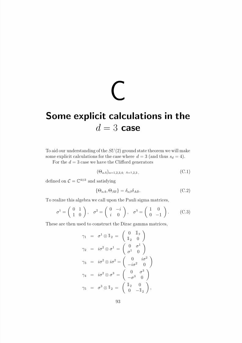
8/3/2019 Ronnie Jansson- The Membrane Vacuum State
http://slidepdf.com/reader/full/ronnie-jansson-the-membrane-vacuum-state 99/107
C
Some explicit calculations in thed = 3 case
To aid our understanding of the SU (2) ground state theorem we will makesome explicit calculations for the case where d = 3 (and thus sd = 4).
For the d = 3 case we have the Clifford generators
(ΘαA)α=1,2,3,4; A=1,2,3 , (C.1)
defined on C = C4⊗3 and satisfying
ΘαA, ΘβB = δαβ δAB. (C.2)
To realize this algebra we call upon the Pauli sigma matrices,
σ1 =
0 11 0
, σ2 =
0 −ii 0
, σ3 =
1 00 −1
. (C.3)
These are then used to construct the Dirac gamma matrices,
γ 1 = σ1
⊗1 2 = 0 1 2
1
2 0 γ 2 = iσ2 ⊗ σ1 =
0 σ1
σ1 0
γ 3 = iσ2 ⊗ iσ2 =
0 iσ2
−iσ2 0
γ 4 = iσ2 ⊗ σ3 =
0 σ3
−σ3 0
γ 5 = σ3 ⊗ 1 2 =
1 2 00 −1 2
,
93
8/3/2019 Ronnie Jansson- The Membrane Vacuum State
http://slidepdf.com/reader/full/ronnie-jansson-the-membrane-vacuum-state 100/107
94 Chapter C Some explicit calculations in the d = 3 case
which we note are all real and anticommute. These matrices now pave
the way for the ΘαA-matrices,
Θα1 =1√
2(γ α ⊗ 1 4 ⊗ γ 5)
Θα2 =1√
2(γ 5 ⊗ γ α ⊗ 1 4)
Θα3 =1√
2(1 4 ⊗ γ 5 ⊗ γ α) ,
which are real 64 × 64 matrices and realize the (C.2) algebra.To describe the fermionic states |F (E, e) we form the two complex
vectors n±, satisfying
n+ · n− = 1 (C.4)
e × n± = in±, (C.5)
and hence also
n± · n± = 0 (C.6)
n+ × n− = −ie. (C.7)
To write down the explicit forms of n± we need an expression for thevector e. To make it simple for us we set e = (1, 0, 0) (we can performarbitrary rotations of this vector afterwards). We then make the ansatz,
n+ = (0, r(cos ρ + i sin ρ), r(− sin ρ + i cos ρ)) (C.8)
n− =
0,
1
2r(cos ρ − i sin ρ), −r
1
2r(sin ρ + i cos ρ)
, (C.9)
and proceed by checking the relations (C.4)-(C.7):
n+ · n− =1
2(cos2 ρ + sin2 ρ + cos2 ρ + sin2 ρ) = 1 (C.10)
e × n+ = (0, r(− sin ρ − i cos ρ), r(cos ρ + i sin ρ)) = −in+ (C.11)
e × n− = (0,1
2r(sin ρ + i cos ρ),
1
2r(cos ρ − i sin ρ)) = in− (C.12)
n+ · n+ = r2(cos2 ρ − sin2 ρ + 2i sin ρ cos ρ+sin2 ρ − cos2 ρ − 2i sin ρ cos ρ) = 0 (C.13)
n− · n− =1
4r2(cos2 ρ − sin2 ρ − 2i sin ρ cos ρ
+sin2 ρ − cos2 ρ + 2i sin ρ cos ρ) = 0 (C.14)
n+ × n− = (−1
2(cos ρ sin ρ + i cos2 +i sin2 ρ − sin ρ cos ρ
− sin ρ cos ρ + i sin2 ρ + i cos2 ρ + cos ρ sin ρ, 0, 0)
= (−i, 0, 0) = −ie. (C.15)
8/3/2019 Ronnie Jansson- The Membrane Vacuum State
http://slidepdf.com/reader/full/ronnie-jansson-the-membrane-vacuum-state 101/107
Some explicit calculations in the d = 3 case 95
In the spirit of explicitness, we write down specific forms of the unit
vectors e and E for the case of d = 9, compliments of [55],
e =
sin θ cos φ
sin θ sin φcos θ
, (C.16)
and
E =
sin 8 sin 7 . . . sin 2 sin 1sin 8 sin 7 . . . sin 2 cos 1
sin 8 sin 7 . . . cos 2...
sin 8 cos 7cos 8
. (C.17)
8/3/2019 Ronnie Jansson- The Membrane Vacuum State
http://slidepdf.com/reader/full/ronnie-jansson-the-membrane-vacuum-state 102/107
96 Chapter C Some explicit calculations in the d = 3 case
8/3/2019 Ronnie Jansson- The Membrane Vacuum State
http://slidepdf.com/reader/full/ronnie-jansson-the-membrane-vacuum-state 103/107
8/3/2019 Ronnie Jansson- The Membrane Vacuum State
http://slidepdf.com/reader/full/ronnie-jansson-the-membrane-vacuum-state 104/107
[14] A. Hanson, T. Regge and C. Teitelboim, Constrained Hamiltonian
Systems. Accademia Nazionale Dei Lincei, Roma, 1976.
[15] P.A. Collins and R. W. Tucker, Classical and quantum mechanicsof free relativistic membranes, Nucl. Phys. B112, 150 (1976).
[16] Bengt E.W. Nilsson, Introduction to supersymmetry. Unpublished,2002.
[17] S. P. Martin, A supersymmetry primer , hep-th/9709356.
[18] J. D. Lykken, Introduction to supersymmetry , hep-th/9612114.
[19] S. Coleman and J. Mandula, All possible symmetries of the S matrix , Phys. Rev. 159, 1251 (1967).
[20] R. Haag, J. Lopuszanski and M. Sohnius, All possible generators of supersymmetries of the S matrix , Nucl. Phys. B88, 257 (1975).
[21] P. S. Howe and E. Sezgin, Superbranes, hep-th/9607227.
[22] P. S. Howe and R. W. Tucker, A locally supersymmetric and reparametrization invariant action for a spinning membrane, J.Phys. 10, L155 (1977).
[23] E. Bergshoeff and E. Sezgin, On ”spinning” membrane models,Phys. Lett. B209, 451 (1988).
[24] J. A. Bagger, The status of supersymmetry , hep-ph/9508392.
[25] H. Baer, C. Balazs and J. K. Mizukoshi, The complementary rolesof the LHC and the LC in discovering supersymmetry ,hep-ph/0111029.
[26] Bengt E.W. Nilsson, Lectures on string theory. Unpublished, 2002.
[27] A. Achucarro, J. M. Evans, P. K. Townsend and D. L. Wiltshire,Super p-branes, Phys. Lett. B198, 441 (1987).
[28] E. Bergshoeff, E. Sezgin and P. Townsend, Supermembranes and eleven-dimensional supergravity , Phys. Lett. B189, 75 (1987).
[29] E. Bergshoeff, E. Sezgin and P. Townsend, Properties of theeleven-dimensional supermembrane theory , Ann. Phys. 185, 330(1987).
[30] J. Goldstone Unpublished.
98
8/3/2019 Ronnie Jansson- The Membrane Vacuum State
http://slidepdf.com/reader/full/ronnie-jansson-the-membrane-vacuum-state 105/107
[31] E. Bergshoeff, E. Sezgin and Y. Tanii, Hamiltonian formulation of
the supermembrane, Nucl. Phys. B298, 187 (1988).
[32] J. Hoppe, Quantum theory of a massless relativistic surface and a two-dimensional bound state problem , Ph.D. Thesis, MIT (1982).
[33] J. Hoppe, Membranes and matrix models, hep-th/0206192.
[34] J. Hoppe, Diff a(t2) and the curvature of some infinite dimensional manifolds, Phys. Lett. B201, 237 (1988).
[35] M. Bordemann, E. Meinrenken and M. Schlichenmaier, Toeplitz quantization of K¨ ahler manifolds and gl(n),n
→ ∞limits.,
Commun. Math. Phys. 165, 281 (1994) [hep-th/9309134].
[36] W. Taylor, Lectures on D-branes, gauge theory and (M)atrices,hep-th/9801182.
[37] J. Polchinski, TASI lectures on D-branes, hep-th/9611050.
[38] E. Floratos and J. Iliopoulos, A note on the classical symmetries of the closed bosonic membranes, Phys. Lett. B215, 706 (1988).
[39] M. Luscher, Some analytic results concerning the mass spectrum of yang-mills gauge theories on a torus, Nucl. Phys. B219, 233(1983).
[40] H. Ooguri and Z. Yin, Lectures on perturbative string theories,hep-th/9612254.
[41] A. Sen, An introduction to non-perturbative string theory ,hep-th/9802051.
[42] M. Kaku, Strings, Conformal Fields, and M-Theory . SpringerVerlag, 2002.
[43] M. J. Duff, A layman’s guide to M-theory , hep-th/9805177.[44] P. K. Townsend, The eleven-dimensional membrane revisited ,
Phys. Lett. B350, 184 (1995).
[45] T. Banks, W. Fischler, S. H. Shenker and L. Susskind, M-theory asa matrix model: A conjecture, Phys. Rev. D55, 5112 (1997)[hep-th/9610043].
[46] L. Susskind, Another conjecture about M(atrix) theory ,hep-th/9704080.
99
8/3/2019 Ronnie Jansson- The Membrane Vacuum State
http://slidepdf.com/reader/full/ronnie-jansson-the-membrane-vacuum-state 106/107
[47] M. Douglas and H. Ooguri, Why matrix theory is hard ,
hep-th/9710178.
[48] W. Taylor, M(atrix) theory: Matrix quantum mechanics as a fundamental theory , Rev. Mod. Phys. (2001) [hep-th/0101126].
[49] T. Banks, Tasi lectures on Matrix theory , hep-th/9911068.
[50] J. Hoppe, On zero-mass bound states in super-membrane models,hep-th/9609232.
[51] J. Frohlich and J. Hoppe, On zero-mass ground states in super-membrane matrix models, Comm. Math. Phys. 191, 613
(1998) [hep-th/9701119].
[52] J. Hoppe, On the construction of zero energy states in supersymmetric matrix models, hep-th/9709132.
[53] J. Hoppe, On the construction of zero energy states in supersymmetric matrix models II , hep-th/9709217.
[54] J. Hoppe, On the construction of zero energy states in supersymmetric matrix models III , hep-th/9711033.
[55] G. M. Graf and J. Hoppe, Asymptotic ground state for 10
dimensional reduced supersymmetric su(2) Yang Mills theory ,hep-th/9805080.
[56] M. Bordemann, J. Hoppe and R. Suter, Zero energy states for su(n): A simple excercise in group theory? , hep-th/9909191.
[57] J. Hoppe, Asymptotic zero energy states for su(n ≥ 3),hep-th/9912163.
[58] J. Hoppe and J. Plefka, The asymptotic groundstate of su(3)matrix theory , hep-th/0002107.
[59] G. M. Graf, D. Hasler and J. Hoppe, No zero energy states for thesupersymmetric x2y2 potential , hep-th/0109032.
[60] D. Hasler and J. Hoppe, Asymptotic factorisation of theground-state for su(n)-invariant supersymmetric matrix-models,hep-th/0206043.
[61] D. Hasler and J. Hoppe, Zero energy states of reduced super Yang-Mills theories id d + 1 = 4, 6 and 10 dimensions arenecessarily Spin( d) invariant , hep-th/0211226.
100
8/3/2019 Ronnie Jansson- The Membrane Vacuum State
http://slidepdf.com/reader/full/ronnie-jansson-the-membrane-vacuum-state 107/107
[62] M. Halpern and C. Schwartz, Asymptotic search for ground states
of su(2) matrix theory , Int. J. Mod. Phys. A13, 4367 (1998)[hep-th/9712133].
[63] J. Wosiek, Spectra of supersymmetric Yang-Mills quantum mechanics, Nucl. Phys. B644, 85 (2002) [hep-th/0203116].
[64] J. Wosiek, Supersymmetric Yang-Mills quantum mechanics, inProceedings of the NATO Advanced Research Workshop on Confinement, Topology and Other Non-Perturbative Aspects of QCD , J. Greensite and S. Olejnik, eds. Kluwer AP, Dordrecht,2002. hep-th/0204243.
[65] J. Wosiek, Recent progress in supersymmetric Yang-Mills quantum mechanics in various dimensions, hep-th/0309174.
[66] P. Yi, Witten index and threshold bound states of d-branes, Nucl.Phys. B505, 307 (1997) [hep-th/9704098].
[67] S. Sethi and M. Stern, D-brane bound states redux , Commun.Math. Phys. 194, 675 (1998) [hep-th/9705046].
[68] H. L. Carrion, M. Rojas and F. Toppan, Quaternionic and octonionic spinors. A classification., hep-th/0302113.
[69] U. Gran, Strings, membranes and supergravity , Master’s thesis,Chalmers University of Technology and Goteborg University, 1996.
[70] M. Nakahara, Geometry, Topology and Physics, Graduate Student Series in Physics. IOP Publishing, 1990.