Root Cause Analysis of Mobile Site

Outage Using Bayesian Network: the

Case of ethio telecom

by : mesfin geremew

adviser : ephrem teshale (phd)

A Thesis submitted to

School of Electrical and Computer Engineering

Addis Ababa Institute of Technology

in Partial Fulfillment of the Requirements for the Degree of Master of Science

(Telecommunication Engineering)

Addis Ababa University

Addis Ababa, Ethiopia

November 17, 2018

Declaration

I, the undersigned, declare that the thesis comprises my own work in compliance

with internationally accepted practices; I have fully acknowledged and referred all

materials used in this thesis work.

Mesfin Geremew

NameSignature

Approved by

Addis Ababa University

Addis Ababa Institute of Technology

School of Electrical and Computer Engineering

This is to certify that the thesis prepared by Mesfin Geremew, entitled Root Cause

Analysis of Mobile Site Outage Using Bayesian Network: the Case of ethio telecom and sub-

mitted in partial fulfillment of the requirements for the degree of Master of Science

(Telecommunication Engineering) complies with the regulations of the University and

meets the accepted standards with respect to originality and quality.

Signed by the Examining Committee:

Internal Examiner Signature Date

Internal Examiner Signature Date

External Examiner Signature Date

Adviser Ephrem Teshale (PhD) Signature Date

Dean, School of Electrical and Computer

Engineering

... for my family

Kid, wife

Nathan, son

A B S T R A C T

In most cellular networks Trouble Shooting (TS) is a manual process, accom-

plished by Radio Access Network (RAN) experts. Their task is to resolve problems

in the network that have been identified by other employees or by automated

checking routines. During the TS procedure, several applications and databases

have to be queried to analyze performance indicators, cell configuration and

alarms of the cells. For example when an outage in mobile network investigated,

a Trouble Ticketing (TT) reflects the problem status, which is the fault descrip-

tion. A TT system is deployed as a large database, which can be queried by the

user, using criteria like time constraints or identifiers, such as site ID (site iden-

tity). After a query, all the cases related to the specified site within the given time

period are shown. The entries are normally in “free text”, almost like a “virtual

log-book” that everyone uses to annotate the actions taken and observations made

for the site. Hence, in difficult cases lots of people from various departments have

looked into the site and potentially applied some changes. For example a case

might involve changing parameters or swapping hardware. Thus, several notes

are normally written to such a case.

The availability of mobile services without interruption has many social and eco-

nomic benefits. However, mobile network outages occur due to many different

reasons. One of the reasons for Base Transceiver Station (BTS) site outage is failure

of hardware elements of the most varied kinds: switching units, cables, cooling

elements, energy elements, etc. The possible relations or interconnections between

elements are not explicitly well-defined so study the root causes of network out-

age is important.

In telecom network environment, there are different network problems of which

their associated causes can be address through Artifitial Intelegent (AI), mostly

detection, and forecasting. On the other hand incident management systems (also

called Trouble Ticket (TT)) have hardly used AI techniques to optimize the pro-

cesses involved. Thus this thesis work investigate the root causes of network out-

age using Bayesian network models, then analyzing the ethio telecom (ET) network

outage TT data.

The outcome for the analysis result are model based Root Causes Analysis of

BTS mobile site network outage is performed, the network technicians can be in-

formed of the real scope of failures and the probable existence of root problems,

technicians can be advantages through managing the situations and good for de-

cision making task by providing the root causes of alarms and their probabilities

of occurrence.

K E Y W O R D S

Network outage, Bayesian Networks, Root cause analysis, Cellular mobile net-

work, Trouble Ticketing, Probability of failure, Model

A C K N O W L E D G M E N T S

Foremost, I would like to express my sincere gratitude to almighty God since am

the son of him.

Thanks to my advisor Ephrem Teshale (PhD) for his continuous support and fol-

low up on my research.

My sincere thanks also go to my friend Biny, for offering me some ideas on ma-

chine learning and Artificial Intelligent (AI) technology.

Last but not the least, I would like to thank all my friends, family and Nathan

Mesfin (son). And also thanks to my parents Babiye and Enaney, for supporting

me spiritually throughout my life.

C O N T E N T S

1 introduction 1

1.1 Statement of the Problem . . . . . . . . . . . . . . . . . . . . . . . . . . . 3

1.2 Objective . . . . . . . . . . . . . . . . . . . . . . . . . . . . . . . . . . . . . 4

1.2.1 General Objective . . . . . . . . . . . . . . . . . . . . . . . . . . . . . . . 4

1.2.2 Specific Objectives . . . . . . . . . . . . . . . . . . . . . . . . . . . . . . 4

1.3 Scope and Limitations . . . . . . . . . . . . . . . . . . . . . . . . . . . . . 5

1.4 Contributions of the research . . . . . . . . . . . . . . . . . . . . . . . . . 5

1.5 Literature Review . . . . . . . . . . . . . . . . . . . . . . . . . . . . . . . . 6

1.6 Methodology . . . . . . . . . . . . . . . . . . . . . . . . . . . . . . . . . . . 6

1.7 Thesis Organization . . . . . . . . . . . . . . . . . . . . . . . . . . . . . . . 7

2 cellular mobile networks 9

2.1 Overview of cellular mobile network systems . . . . . . . . . . . . . . . . 9

2.2 Interconnection of equipment’s in BTS sites . . . . . . . . . . . . . . . . . 11

2.3 Cellular Network management . . . . . . . . . . . . . . . . . . . . . . . . 12

2.4 Troubleshooting in cellular networks . . . . . . . . . . . . . . . . . . . . . 13

3 root cause analysis techniques 16

3.1 Introduction . . . . . . . . . . . . . . . . . . . . . . . . . . . . . . . . . . . 16

3.2 Reasoning under uncertainty . . . . . . . . . . . . . . . . . . . . . . . . . 20

3.2.1 Introduction . . . . . . . . . . . . . . . . . . . . . . . . . . . . . . . . . . 20

3.2.2 Probabilistic networks . . . . . . . . . . . . . . . . . . . . . . . . . . . . 20

3.2.3 Justification of the selected technique/Algorithms overview . . . . . . 22

3.3 Bayesian Networks . . . . . . . . . . . . . . . . . . . . . . . . . . . . . . . 23

3.3.1 Introduction to Bayesian Network (BN)s . . . . . . . . . . . . . . . . . . 23

3.3.2 The chain rule and Bayes theorem for BNs . . . . . . . . . . . . . . . . 25

3.3.3 Bayesian modeling . . . . . . . . . . . . . . . . . . . . . . . . . . . . . . 26

3.3.4 BN Learning . . . . . . . . . . . . . . . . . . . . . . . . . . . . . . . . . . 27

contents ix

4 analysis of bts site network outage 28

4.1 Introduction . . . . . . . . . . . . . . . . . . . . . . . . . . . . . . . . . . . 28

4.1.1 Basic definitions . . . . . . . . . . . . . . . . . . . . . . . . . . . . . . . . 28

4.2 Causes of network outage . . . . . . . . . . . . . . . . . . . . . . . . . . . 29

4.2.1 Hardware . . . . . . . . . . . . . . . . . . . . . . . . . . . . . . . . . . . 29

4.2.2 Transmission . . . . . . . . . . . . . . . . . . . . . . . . . . . . . . . . . . 30

4.2.3 Power system failure . . . . . . . . . . . . . . . . . . . . . . . . . . . . . 31

4.2.4 Other failures . . . . . . . . . . . . . . . . . . . . . . . . . . . . . . . . . 32

5 case study 34

5.1 System Introduction . . . . . . . . . . . . . . . . . . . . . . . . . . . . . . 34

5.2 Discrete Failure Distribution . . . . . . . . . . . . . . . . . . . . . . . . . . 35

5.2.1 Fault Tree Analysis Approach . . . . . . . . . . . . . . . . . . . . . . . . 35

5.2.2 Bayesian Network Approach . . . . . . . . . . . . . . . . . . . . . . . . 36

6 bayesian network model and analysis results 39

6.1 Model based on Bayesian Networks . . . . . . . . . . . . . . . . . . . . . 39

6.2 Bayesian Networks Learning . . . . . . . . . . . . . . . . . . . . . . . . . 42

6.2.1 Code / BNT class structure . . . . . . . . . . . . . . . . . . . . . . . . . 43

6.2.2 Parameter learning . . . . . . . . . . . . . . . . . . . . . . . . . . . . . . 43

7 conclusion and recommendation 45

7.1 Conclusion . . . . . . . . . . . . . . . . . . . . . . . . . . . . . . . . . . . . 45

7.2 Recommendation . . . . . . . . . . . . . . . . . . . . . . . . . . . . . . . . 46

references 47

a appendix-i 51

L I S T O F F I G U R E S

Figure 2.1 Interconnection of equipment’s in BTS sites . . . . . . . . . . 11

Figure 2.2 Troubleshooting in current mobile communication networks 15

Figure 3.1 Five basic steps for complete RCA . . . . . . . . . . . . . . . 17

Figure 3.2 Simple Bayesian Network example . . . . . . . . . . . . . . . 21

Figure 3.3 serial connection . . . . . . . . . . . . . . . . . . . . . . . . . . 23

Figure 3.4 diverging connection . . . . . . . . . . . . . . . . . . . . . . . 23

Figure 3.5 converging connection . . . . . . . . . . . . . . . . . . . . . . 24

Figure 3.6 A simple Bayesian network . . . . . . . . . . . . . . . . . . . . 25

Figure 4.1 Power systems for BTS sites . . . . . . . . . . . . . . . . . . . 31

Figure 5.1 Fault Tree Structure for BTS Network . . . . . . . . . . . . . . 36

Figure 5.2 Transformed fault tree to Bayesian Network Structure . . . . 37

Figure 6.1 Generated Bayesian Networks Structure . . . . . . . . . . . . 40

Figure 6.2 Conditional probability of IDU, ODU, Ant1, Link1 and conf1

given Nout=1 . . . . . . . . . . . . . . . . . . . . . . . . . . . . 41

Figure 6.3 Conditional probability of parent nodes given Nout=1 . . . . 41

Figure 6.4 BN Learning from TT data . . . . . . . . . . . . . . . . . . . . 44

Figure 6.5 Training from DAG and ns . . . . . . . . . . . . . . . . . . . . 44

Figure A.1 system model . . . . . . . . . . . . . . . . . . . . . . . . . . . 54

Figure A.2 Fault distribution . . . . . . . . . . . . . . . . . . . . . . . . . 54

Figure A.3 leveled dataset . . . . . . . . . . . . . . . . . . . . . . . . . . . 56

L I S T O F TA B L E S

Table 3.1 Comparison of classification algorithms . . . . . . . . . . . . 22

Table 6.1 Conditional probability distribution for the five components 40

Table A.1 Parent nodes definition . . . . . . . . . . . . . . . . . . . . . . 51

Table A.2 Leveling the dataset . . . . . . . . . . . . . . . . . . . . . . . . 55

Table A.3 Expertise thought . . . . . . . . . . . . . . . . . . . . . . . . . 55

A C R O N Y M S

AC Alternating Current

AI Artifitial Intelegent

Ant Antenna

ASCII American Standard Code for Information Interchange

ATN Aeronautical Telecommunication Network

BBU Baseband Unit

BN Bayesian Network

BNT Bayesian Network Toolbox

BSC Base Station Controller

BTS Base Transceiver Station

CPD Conditional Probability Distribution

CPT Conditional Probability Table

CPU Central Processing System

DAG Directed Acyclic Graph

DG Diesel Generator

DT Decision Trees

ET ethio telecom

EM Expectation Maximization

FT Fault Tree

FTA Fault Tree Analysis

acronyms xiii

HLR Home Location Register

IDU Indoor Unit

IT Information Technology

ISO Internation Organization for Standardization

ITU International Telecommunication Union

KNN K-Nearest Neighbors

KPI Key Performance Indicator

MPD Marginal Probability Distribution

MSC Mobile Switching Center

MW Microwave

NMS Network Management System

NOC National Operation Center

OM Operation and Maintenance

ODU Outdoor Unit

Opt Optical

OSI Open Systems Interconnect

PDF Probability Density Functions

PSTN Public Switched Telephone Network

QoS Quality of Service

RAN Radio Access Network

RCA Root Cause Analysis

RRU Remote Radio Unit

SVM Support Vector Machines

TE Top Event

acronyms xiv

Tr Transmission

TRX Transceivers (Transmitter/Receiver)

TS Trouble Shooting

TT Trouble Ticket

UE User Equipment

VLR Visitor Location Register

1I N T R O D U C T I O N

Telecom network consists of thousands of different hardware elements of the most

varied kinds: base stations, servers, routers, modems, switching units, cables, cool-

ing elements, energy elements, etc. The possible relations between elements are

not explicitly well-defined [1], [2]. As an example, the relationship between the

cooling system that controls a room temperature and all the hardware installed in

the room is not defined though a failure in the air conditioner will probably af-

fect a smooth running of the hardware. Another example is a fiber cut that makes

many dependent mobile base stations to be turned off, accordingly affecting many

customers. This makes it difficult to use traditional programming solutions to au-

tomatically link failures to a root cause incident management systems, also known

as Trouble Ticket (TT) systems, which provides a clue to the technician the pos-

sibility to link an incident produced on an element to another existing incident,

creating a child-parent relation. So, it depends on expert knowledge to be able to

identify these situations quickly. The discovery of the root cause of a real prob-

lem can take much time and resources to analyze them and it is a challenge for

technicians. In the meantime many customers could have their services partially

or fully affected. In contrary, what is important is predicting how a failure in an

element can affect other elements, thus being able to evaluate the real scope of the

problem as soon as possible.

Root Cause Analysis (RCA) is a step-by-step method that leads to the discovery

of a fault’s or root cause [3]. Every equipment failure happens for a number of

reasons. There is a definite progression of actions and consequences that lead to a

failure. An RCA traces the cause and effect trail from the end failure back to the

root cause.

Useful tools to determine root cause are First, the "Five why’s" refers to the prac-

tice of asking, five times, why the failure has occurred in order to get the root

introduction 2

cause/causes of the problem. Five why’s are best used when tackling a simple

RCA. secondly, "Tree diagram" is a graphical technique uses Boolean logic to de-

termine the cause of problem in any undesirable event. As the name implies, this

tool involves creating a diagram that looks like trees where all potential causes

are written down as branches. The third one is "Cause and effect", also called Fish

bone diagram (for their appearance) and Ishikawa diagram (by the name of de-

veloper), identifies all the potential processes and factors that could contribute to

a problem. Once the information is obtained, try and priorities those areas that

you have a control over, and concentrate on finding resolutions for these. It is

used for more complex Root Cause Analysis. Finally, "Brainstorming", is a situa-

tion where group of people meet to generate new ideas and solutions around a

specific domain of interest by removing inhibitions. People are able to think more

freely and they suggest many spontaneous new ideas as possible. This thesis will

use Bayesian network model which has a concept for all the four useful tools; the

thesis uses matlab as a tool.

In telecoms network environment, there are a variety of Artificial Intelligent (AI)

approaches to address different problems mostly in detection and forecasting of

network outages [4]. However, incident management systems (also called trouble

ticket (TT)) have hardly used AI techniques to optimize the processes involved.

Most of the time optimizations are reduced to more or less sophisticated deci-

sion rules, or searching for previous similar cases in knowledge bases in what

is known as case based reasoning [2]. For complex and changing environment,

machine learning techniques are applied in the context of TT systems to discover

information and automate certain tasks [5].

For large heterogeneous network; an incident could affect an important service

offered to hundreds of people, thousands of incidents may appear every day, and

the topology of network is complex [6], [7]. Under these conditions, decisions can-

not be delayed and actions must be carried out right away.

Currently, Bayesian networks BNs have had a revival within the AI community.

BN’s causal semantics allows the representation of causal relationships between

the variables. BNs model the quantitative strength of the connections between

variables, allowing probabilistic beliefs about them to be updated automatically

as new information becomes available. This allows inference and reasoning under

1.1 statement of the problem 3

uncertainty, probabilistically, in what is called Bayesian reasoning. As BNs provide

full representations of probability distributions over their variables, they can be

conditioned upon any subset of them, supporting any direction of reasoning. For

example, diagnostic reasoning, that goes from symptoms observed to causes; or

predictive reasoning, that goes from new information about causes to new beliefs

about effects. All this makes BNs a good AI technique to address the problem of

finding the root cause of an incident in telecom networks [8].

1.1 statement of the problem

Telecommunication sector has considerably large network infrastructure and also

making continuous network expansions with large amount of investments. Cur-

rently, ethio telecom’s mobile network capacity reaches 62 million which has 85%

mobile coverage [9], [10]. However, as an operator, ethio telecom is facing chal-

lenges like network unavailability across various networks. From these various

networks, mobile network daily outage share is the largest, which is around 67%,

among the total down sites [11].

What is even worse is that, most faults sustain unsolved for more than three days

in which their associated cost is high in terms of revenue loss during service in-

terruption, increasing maintenance cost and Quality of Service (QoS) are impacted.

Therefore, analyzing the root cause of mobile network outages are important to

understand the characteristic (behavior) of faults.

The basic problem motivating this thesis work is that RCA is an extremely time-

consuming, and it’s also an expensive process. The speed in identifying faults is

dependent on the level of expertise of the troubleshooter, the type of informa-

tion available and the quality of tools displaying relevant pieces of information.

This means that, in addition to a good understanding of the possible causes of the

problems, a very good understanding of the tools available to access the sources of

information is also required. Currently the most common way of analyzing what

has happened in the ethio telecom base station is to take log files, and manually

look for anything that is seemingly alarming.

Some literatures [8], [12], [13] can be found on automatic diagnosis of faults in

1.2 objective 4

telecom networks. Based on this, the selected technique in this thesis has been

Bayesian Network. BNs, also called belief probabilistic networks, have been pro-

posed by many authors as the modeling technique for the development of au-

tomatic diagnosis systems. Moreover, their polyvalence that dealing with issues

such as prediction or diagnosis, optimization, data analysis of feedback experi-

ence, deviation detection and model updating, able to represent graphically and

necessity of deep understanding of the cause and effect relationships in a domain.

1.2 objective

1.2.1 General Objective

The main objective of this thesis work is to investigate the root cause of BTS mobile

network outage in Addis Ababa using Bayesian network.

1.2.2 Specific Objectives

The specific objectives of this thesis are summarized as follows:

• Identify key models and methods used in the area of RCA in telecom net-

works;

• Analysis of the mobile site outage Trouble Ticket (TT) data for ethio telecom

cases by those selected models;

• To define the causes for outage and the probable existence of root problems;

• To discover the hidden dependencies between elements and;

• To support the operator in their decision making task by providing the root

causes of alarms and their probabilities of occurrence.

1.3 scope and limitations 5

1.3 scope and limitations

The scopes of this thesis are:

• Investigate the root cause of BTS mobile network outage using Bayesian

network model.

• Providing probabilities of occurrence for alarm system that supports the

operator in their decision making task.

The limitation of this thesis are:

• The training data was limited to one month, because of unmanaged TT data.

• The TT data are collected on one vendor BTS mobile equipment . So that the

interconnection between nodes and their probable existence of outage may

be different from other vendor having different equipment.

1.4 contributions of the research

The contributions of this thesis are:

• Model based Root Causes Analysis of BTS mobile site network outage is

performed.

• The network technicians can be informed of the real scope of failures and the

probable existence of root problems, thus optimizing resources and reducing

recovery time.

• Technicians can be advantages through managing the situations.

• Good for decision making task by providing the root causes of alarms and

their probabilities of occurrence.

1.5 literature review 6

1.5 literature review

Bayesian networks are widely used in many fields. There are a lot of practical ap-

plications of Bayesian networks. In machine learning and data mining fields, the

Bayesian network has been a hot topic for many years, especially in the root cause

analysis of network outage [4], [8], [14], [15].

Regarding the Root Cause Analysis of telecom networks, Fco. Velasco presents the

importance of using TT record data as an input to the BN model [8]. Then dene

different rules/threshold and applied to warm engineers for different situations

for Root Cause Analysis.

Design of an automatic diagnosis of cellular networks system for the RAN seg-

ment of GSM/GPRS networks and BN modeling of Call drop are presented by

Michael W. using methods based on data or on a combination of data and ex-

pertise [16]. The algorithm used for probability denition has proven to be more

important than the method used to calculate the thresholds.

Finally Lisa, et al. proposes architecture for the alarm system by combining knowl-

edge modeling and machine learning for alarm root cause analysis using Bayesian

network [15]. The knowledge engineer has to collect, structure, and model the

expert knowledge; in doing these tasks time and effort consuming that might

increase with the complexity of the industrial plant to be modeled which are lan-

guage dependent and have to be translated to other languages if needed. On the

other hand, the machine learning approach benets from several advantages that

BNs are faster to build by learning, scalable and language independent.

1.6 methodology

This thesis is entirely based on ethio telecom BTS mobile network site. The work

started with a survey on how troubleshooting is currently performed in exist-

ing cellular networks, deep understanding of the equipment’s found in the BTS

mobile site and then try to perform the causality between equipment’s and find

1.7 thesis organization 7

out the probability of fault occurrence using Bayesian Network model based. Af-

ter that, root cause analyses have been done to identify the probability of nodes

available in the BTS site network. The analysis results can help for those decision

makers to take action.

In general the method is formulated as:

• Survey on existing cellular networks;

• Discussions are made with RAN expertise;

• Collect alarm history data, TT, from ethio telecom network performance sec-

tion;

• Select the appropriate model for the RCA of network outage;

• Application of BNs will be presented;

– Bayes rule

– Model the causality relations among variables

– Leveling the TT dataset as per our nodes or elements.

– Bayesian learning and inference takes place on nodes.

• Presents the nal results obtained using matlab and

• Finally, the conclusions for the analysis

1.7 thesis organization

The organization of this thesis work is directly related to the objectives presented

above. Chapter one presents the introduction, statement of the problems, objective

of the thesis, literature review, methodologies, thesis scope and limitation, contri-

bution and thesis layout. Chapter two presents the overview of Cellular mobile

network systems, interconnection of equipment’s in BTS sites, network manage-

ment in cellular networks and troubleshooting in cellular networks. Chapter three

presents Introduction of Root Cause Analysis, Reasoning under uncertainty for

1.7 thesis organization 8

Root cause analysis and Bayesian networks. Chapter four presents the introduc-

tion of network outage and their definitions and Causes of network outage. Chap-

ter five presents ethio telecom case study of system introduction and discrete

failure distribution. Chapter six presents Bayesian network model and analysis

results. Chapter seven presents conclusion followed by points of recommendation.

Finally, presents appendix section for further data collection or preparation.

2C E L L U L A R M O B I L E N E T W O R K S

2.1 overview of cellular mobile network systems

A cellular network is a radio network distributed over land through cells where

each cell includes a fixed location transceiver known as base station. These cells

together provide radio coverage over larger geographical areas. User Equipment

(UE), such as mobile phones, is therefore able to communicate even if the equip-

ment is moving through cells during transmission [17].

Cellular network technology supports a hierarchical structure formed by the Base

Transceiver Station (BTS), Mobile Switching Center (MSC), location registers and

Public Switched Telephone Network (PSTN). The BTS enables cellular devices to

make direct communication with mobile phones. The unit acts as a base sta-

tion to route calls to the destination base center controller. The Base Station Con-

troller (BSC) coordinates with the MSC to interface with the landline-based PSTN,

Visitor Location Register (VLR), and Home Location Register (HLR) to route the

calls toward different base center controllers. A typical cell site offers geographical

coverage of between nine and 21 miles. The base station is responsible for mon-

itoring the level of the signals when a call is made from a mobile phone. When

the user moves away from the geographical coverage area of the base station, the

signal level may fall. This can cause a base station to make a request to the MSC to

transfer the control to another base station that is receiving the strongest signals

without notifying the subscriber; this phenomenon is called handover. Cellular

networks often encounter environmental interruptions like a moving tower crane,

overhead power cables, or the frequencies of other devices.

Wireless Cellular Systems solves the problem of spectral congestion and increases

user capacity.

2.1 overview of cellular mobile network systems 10

The coverage area of cellular networks is divided into cells, each cell having its

own antenna for transmitting the signals. Data communication in cellular net-

works is served by its base station transmitter, receiver and its control unit. The

shape of cells can be either square or hexagon.

Frequency reusing is the concept of using the same radio frequencies within a

given area that are separated by considerable distance, with minimal interference,

to establish communication. For example, when N cells are using the same num-

ber of frequencies and K be the total number of frequencies used in systems. Then

each cell frequency is calculated by using the formulae K/N.

Mobile Wireless Communication networks have experienced a remarkable change.

The mobile wireless Generation (G) generally refers to a change in the nature of

the system, speed, technology, frequency, data capacity, latency etc. Each genera-

tion have some standards, different capacities, new techniques and new features

which differentiate it from the previous one. The first generation (1G) mobile wire-

less communication network was analog used for voice calls only. The second gen-

eration (2G) is a digital technology and supports text messaging. The third gen-

eration (3G) mobile technology provided higher data transmission rate, increased

capacity and provide multimedia support. The fourth generation (4G) integrates

3G with fixed internet to support wireless mobile internet, which is an evolution

to mobile technology and it overcome the limitations of 3G. It also increases the

bandwidth and reduces the cost of resources. 5G stands for 5th Generation Mo-

bile technology and is going to be a new revolution in mobile market which has

changed the means to use cell phones within very high bandwidth.

The following sections are focused on those aspects of mobile networks that are

more related to this thesis. In Section 2.2, the interconnection of equipment’s in

BTS sites will be described. In Section 2.3, Cellular network management will be

summarized. Finally, in Section 2.4, troubleshooting in cellular network will be

introduced.

2.2 interconnection of equipment’s in bts sites 11

2.2 interconnection of equipment’s in bts sites

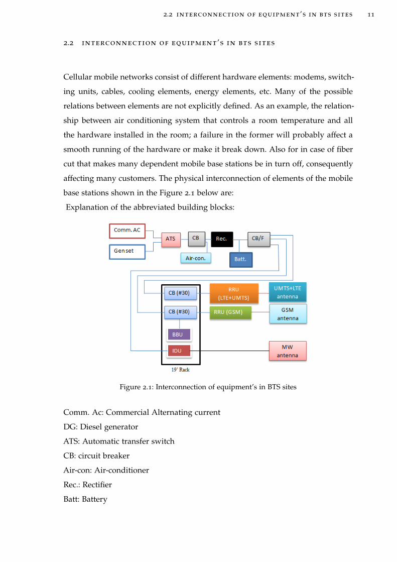
Cellular mobile networks consist of different hardware elements: modems, switch-

ing units, cables, cooling elements, energy elements, etc. Many of the possible

relations between elements are not explicitly defined. As an example, the relation-

ship between air conditioning system that controls a room temperature and all

the hardware installed in the room; a failure in the former will probably affect a

smooth running of the hardware or make it break down. Also for in case of fiber

cut that makes many dependent mobile base stations be in turn off, consequently

affecting many customers. The physical interconnection of elements of the mobile

base stations shown in the Figure 2.1 below are:

Explanation of the abbreviated building blocks:

Figure 2.1: Interconnection of equipment’s in BTS sites

Comm. Ac: Commercial Alternating current

DG: Diesel generator

ATS: Automatic transfer switch

CB: circuit breaker

Air-con: Air-conditioner

Rec.: Rectifier

Batt: Battery

2.3 cellular network management 12

CB/F: Circuit breaker or fuse

BBU: Base band unit

IDU: Indoor unit

RRU: Remote radio unit

MW: microwave

Thus, for the hardware elements that this information is not explicitly modeled, it

is difficult to use traditional programming solutions to automatically link failures

to a root cause.

2.3 cellular network management

RCA is one of the main tasks in network management. Network management

is responsible for the efficient operation and organization of telecom networks.

Internation Organization for Standardization (ISO) together with International

Telecommunication Union (ITU) standardized network management following the

Open Systems Interconnect (OSI) Reference Model [18]. Functional areas defined

by the standard are:

• Fault management, which is responsible for detection, isolation and correc-

tion of network faults.

• Configuration management, which provides the operators with the means to

define, control and monitor network elements in order to maintain a reliable

communication network.

• Accounting management, which deals with managing the billing and charg-

ing system, calculating the cost of network services.

• Performance management, which handles the execution of performance mea-

surements by monitoring and analyzing the managed network elements and

services.

2.4 troubleshooting in cellular networks 13

• Security management, which ensures that the information exchanged by the

network is not corrupted.

Current cellular mobile networks are still requiring significant manual configura-

tion and management for deployment and operation. However, the rapid increase

in complexity and size of the networks being managed have led to a widespread

belief that current management models need to change to meet the challenges of

future ubiquitous networking [19].

To monitor network performance, three sources of information are normally con-

sidered: customer complaints, field tests and statistics in the Network Manage-

ment System (NMS) [20]. Key Performance Indicator (KPI)s which is the most

important parameter amongst network performance indicators, are defined by

network manufacturers in order to allow more efficient performance monitoring.

Apart from KPIs, alarms are generated at several points of the network to indi-

cate a failure. Subsequently, they are transmitted and stored in the NMS. Although

alarms are symptoms of malfunctioning, they do not necessarily point to the exact

cause of the problems.

2.4 troubleshooting in cellular networks

The increase in size, complexity and heterogeneity of evolved networks, need for

an advanced fault management capability becomes critical. Fault management,

also called troubleshooting (TS), includes the detection, isolation and correction

of faults, where a fault is a cause of malfunctioning.

In the current cellular networks, Trouble Shooting (TS) is a manual process carried

out by experts in the Radio Access Network (RAN). This TS process is characterized

by eliminating likely problem causes in order to pick out the actual one. During

the procedure, several applications and databases have to be queried to analyze

performance indicators, cell configurations and alarms. The speed of identifying

faults is dependent on the level of expertise of the troubleshooter, the type of

information available and the quality of the tools displaying relevant pieces of

information. This means that, in addition to a good understanding of the possible

2.4 troubleshooting in cellular networks 14

causes of the problems, a very good understanding of the tools available to access

the sources of information is also required. Due to the complexity of the manage-

ment system, it is almost impossible for newcomers to perform TS in a proficient

manner.

TS in a cellular network consist of the following phases.

• Fault detection: malfunctioning element should be identified based on alarms.

• Diagnosis: the cause of the problems should be identified based on alarms

and configuration data.

• Fault recovery: some actions should be carried out in order to solve the

problems.

This thesis is focused on diagnosis/analysis, which is by far the most difficult and

thus time-consuming task within the TS activity, since for analysis task it needs to

have the detail interconnection of the nodes and their probable existence of failure

in the system.

In operational scenario, when an outage in mobile network is investigated, a TT

indicated the fault description and the steps performed so far to solve it out or

the identification of the faulty equipment in case the problem is believed as a HW

fault. A TT system’s database can be queried by the user, using criteria like time

constraints or site ID. After a query, all the cases related to the specified site within

the given time period are shown.

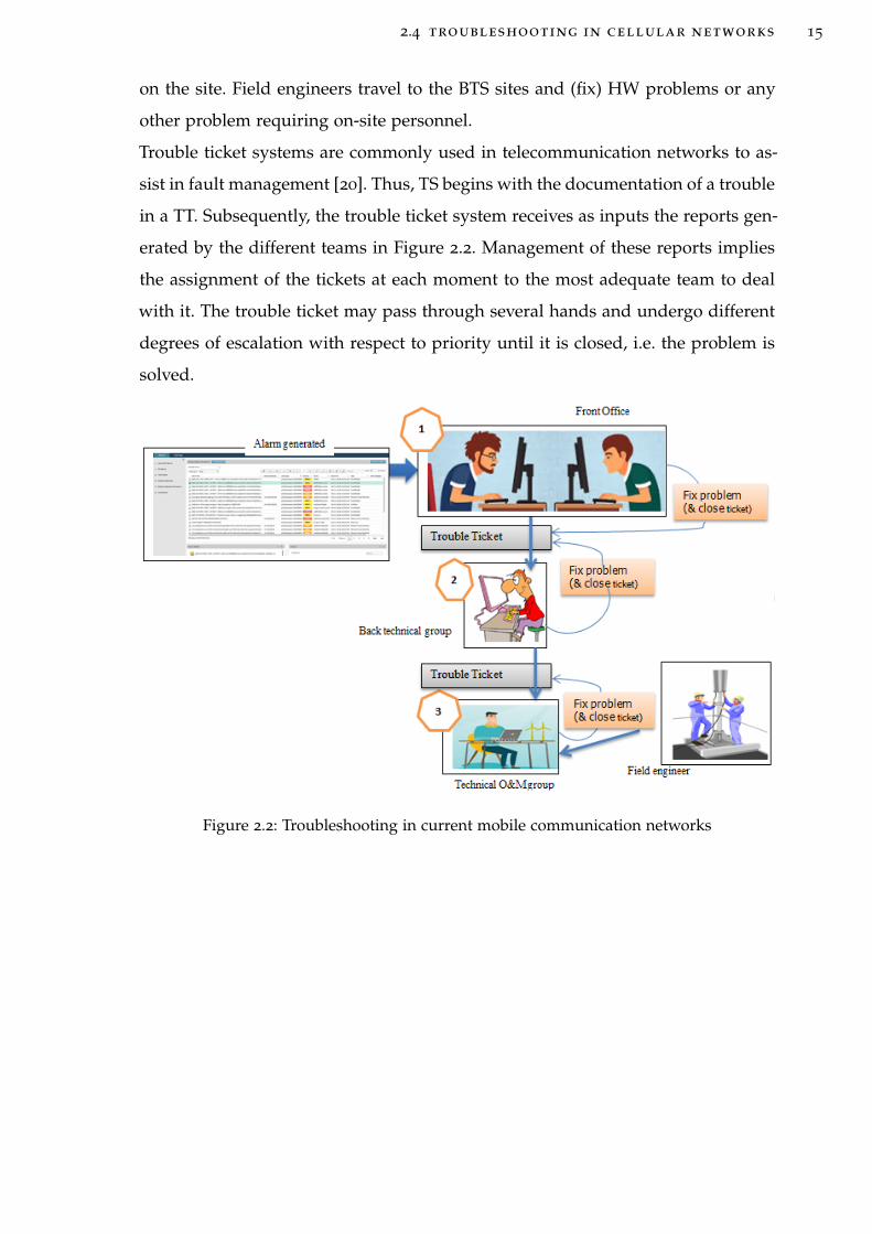
There are different steps required in troubleshooting, as shown in Figure 2.2 below.

The front office group is the first such layer. This team is responsible for dealing

with alarms generated by the network and then raises TT reports related to those

alarms. Then send the TT to the second layer, back technical team, for further in-

vestigation, including in the TT a description of the steps that were carried out.

Back technical group pursue a deeper analysis to identify the cause of the prob-

lem and they update the TT with the executed actions. If, as a consequence, the

problem is solved, they close the TT. If they are not able to solve the problem, they

reassign the TT to a more specialized group, the Technical Operation and Mainte-

nance (OM) group. These technical staffs travel to the site for further solution.

The technical group needs to involve field engineers for problems related to HW

2.4 troubleshooting in cellular networks 15

on the site. Field engineers travel to the BTS sites and (fix) HW problems or any

other problem requiring on-site personnel.

Trouble ticket systems are commonly used in telecommunication networks to as-

sist in fault management [20]. Thus, TS begins with the documentation of a trouble

in a TT. Subsequently, the trouble ticket system receives as inputs the reports gen-

erated by the different teams in Figure 2.2. Management of these reports implies

the assignment of the tickets at each moment to the most adequate team to deal

with it. The trouble ticket may pass through several hands and undergo different

degrees of escalation with respect to priority until it is closed, i.e. the problem is

solved.

Figure 2.2: Troubleshooting in current mobile communication networks

3R O O T C A U S E A N A LY S I S T E C H N I Q U E S

In order to do the root causes of a network problem, we need to have more in-

formation about the network architecture, mechanisms to trigger the collection of

metrics and to constantly monitor the state of all elements that may be involved in

this kind of analysis. When one starts an analysis, it is hard to choose a subset of

elements where we are sure to find the original cause, thus every single element

may have its own importance.

The first part of this Chapter is an introduction, then on section 3.2 summarizes

some techniques which may be used to model uncertainty in reasoning. Lastly,

on section 3.3 devoted to the principles of Bayesian network, which will be the

selected method for this thesis work.

3.1 introduction

RCA is a method that is used to address a problem, to get the “root cause” of

the problem. It is used so we can correct or eliminate the cause and prevent the

problem from recurring.

RCA is simply the application of a series of well known, common sense tech-

niques which can produce a systematic, quantified and documented approach to

the identification, understanding and resolution of underlying causes [21].

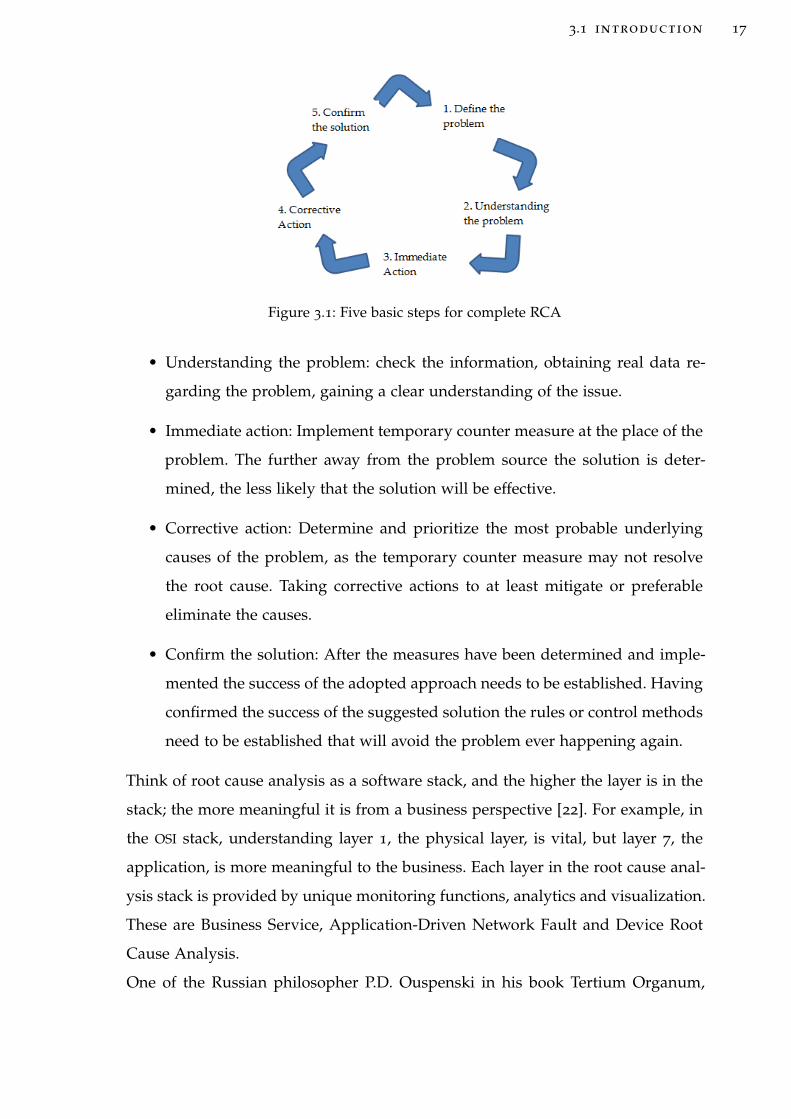
In order to discover the problem, there are five steps to completing the RCA as

shown on Figure 3.1 [21].

• Define the problem: try and use the principles that are specific, measurable,

actions oriented, realistic and time constrained. Unless the problem is de-

fined accurately, the RCA whole process maybe prone to failure.

3.1 introduction 17

Figure 3.1: Five basic steps for complete RCA

• Understanding the problem: check the information, obtaining real data re-

garding the problem, gaining a clear understanding of the issue.

• Immediate action: Implement temporary counter measure at the place of the

problem. The further away from the problem source the solution is deter-

mined, the less likely that the solution will be effective.

• Corrective action: Determine and prioritize the most probable underlying

causes of the problem, as the temporary counter measure may not resolve

the root cause. Taking corrective actions to at least mitigate or preferable

eliminate the causes.

• Confirm the solution: After the measures have been determined and imple-

mented the success of the adopted approach needs to be established. Having

confirmed the success of the suggested solution the rules or control methods

need to be established that will avoid the problem ever happening again.

Think of root cause analysis as a software stack, and the higher the layer is in the

stack; the more meaningful it is from a business perspective [22]. For example, in

the OSI stack, understanding layer 1, the physical layer, is vital, but layer 7, the

application, is more meaningful to the business. Each layer in the root cause anal-

ysis stack is provided by unique monitoring functions, analytics and visualization.

These are Business Service, Application-Driven Network Fault and Device Root

Cause Analysis.

One of the Russian philosopher P.D. Ouspenski in his book Tertium Organum,

3.1 introduction 18

said think of adding each layer in terms of a geometrical analogy of human aware-

ness cleverly. As he explained, if you were one-dimensional, a point, you couldn’t

think of a line. If you were a line, you couldn’t perceive two-dimensions: a square.

If you were a square you couldn’t understand a cube. If you were a cube, couldn’t

understand motion.

The device layer is the foundation, letting you know if a server, storage device or

switch, router, etc. simply is up or down, fast or slow. If it’s pingable, you know

it has a power source, and diagnostics can tell you which subcomponent has the

fault causing the problem. For root cause of performance issues, you’ll be rely-

ing on your monitoring tools’ visual correlation of time series data and threshold

alerts to see if the Central Processing System (CPU), memory, disk, ports etc. are

degraded and why.

But if servers or network devices aren’t reachable, how do you know for sure if

they are down or if there’s an upstream network root cause? To see this, you need

to add a higher layer of monitoring and analytics.

The next layer is Network Root Cause Analysis. This is partly based on a mecha-

nism called inductive modeling, which discovers relationships between networked

devices by discovering port connections and routing and configuration tables in

each device. When an outage occurs, inference, a related Network Root Cause

Analysis mechanism, uses known network relationships to determine which de-

vices are downstream from the one that is down. So instead of drowning in a sea

of red alerts for all the unreachable devices, you get one upstream network root

cause alert. This can also be applied to virtual servers and their underlying physi-

cal hosts, as well as network configuration issues.

Next up is Application-Driven Network Performance Management, which includes

two monitoring technologies: network flow analysis and end-to-end application

delivery analysis.

The first mechanism lets you see which applications are running on your network

segments and how much bandwidth each is using. When users are complaining

that an application service is slow, this can let you know when a bandwidth-

monopolizing application is the root cause. Visualization includes stacked proto-

col charts, top hosts, top talkers, etc.

The second mechanism in this layer shows you end-to-end application response

3.1 introduction 19

timing: network round trip, retransmission, data transfer and server response. To-

gether in a stacked graph, this reveals if the network, the server or the application

itself is impacting response. To see the detailed root cause in the offending do-

main, you drill down into a lower layer (e.g., into a network flow analysis, device

monitoring or an application forensic tool).

The best practice is to unify the three layers into a single infrastructure manage-

ment dashboard, so you can visually correlate all three levels of analytics in an

efficient work flow. This is ideal for technical Level 2 Operations specialists and

administrators. But there’s one more level at the top of the stack: Business Service

Root Cause Analysis. This gives Information Technology (IT) Operations Level 1

staff the greatest insight into how infrastructure is impacting business processes.

Examples of business processes include: concept to product, product to launch,

opportunity to order, order to cash, request to service, design to build, manufac-

turing to distribution, build to order, build to stock, requisition to payables and

so on. At this layer of the stack, you monitor application and infrastructure com-

ponents in groups that support each business process. This allows you to monitor

each business process as you would an IT infrastructure service, and a mechanism

called service impact analysis rates the relative impact each component has on

the service performance. From there you can drill down into a lower layer in the

stack to see the technical root cause details of the service impact (network outage,

not enough bandwidth, server memory degradation, packet loss, not enough host

resources for a virtual server, application logic error, etc)

Once you have a clear understanding of this architecture, and a way to unify the

information into a smooth work flow for triage, you can put the human processes

in place to realize its business value.

3.2 reasoning under uncertainty 20

3.2 reasoning under uncertainty

3.2.1 Introduction

When an expert asserts which was the cause of problems in a mobile network,

he/she is never completely sure about his/her investigation. There are different

sources of uncertainty the data could be unreliable, the data may be incomplete,

the data may be only approximately known and not only might the data be im-

precise, but might be the rules for drawing conclusions. That is, the knowledge

is not deterministic. For example, the same symptoms may be related to different

causes. Therefore, analysis requires a means for reasoning with uncertainty.

There are different approaches to model uncertainty. Most techniques use the the-

ory of probability to deal with uncertainty. There is objective probability, which is

linked to the convergence of a relative frequency of an experiment, and subjective

probability, also called degree of belief, which is an individual’s subjective esti-

mate of the certainty of an event. For example, the experiment of tossing a coin

could be repeated many times and the “objective” probability of any of the out-

comes would be the limit, as the number of trials approach infinity, of the relative

frequency of that outcome. However, if a person has to bet that ‘A’ will be the

winning team on a given upcoming football game, the probability would be “sub-

jective” because the game cannot be repeated many times under the exact same

conditions.

3.2.2 Probabilistic networks

A probabilistic network, also called Bayesian Network is a pair (D, P) that allows

efficient representation of a joint probability distribution over a set of random

variables U = X1, . . . ,Xn [23]. The letter D represents the Directed Acyclic Graph

(DAG), whose nodes correspond to the random variables X1, . . . ,Xn and whose

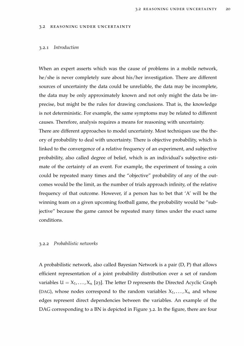
edges represent direct dependencies between the variables. An example of the

DAG corresponding to a BN is depicted in Figure 3.2. In the figure, there are four

3.2 reasoning under uncertainty 21

nodes or variables of X1, X2, X3 and X4. Node X1 is the parent node where as node

X2 and X3 are child nodes for node X1. Node X4 is the child node for X2.

P = p(X1 | π1), . . . ,p(Xn | πn) (3.1)

Where πi is the parent set of Xi.

Figure 3.2: Simple Bayesian Network example

The second component, P, is a set of conditional probability functions, one for each

variable: The set P defines a unique joint probability distribution over U given by

P(U) =

n∏i=1

p(Xi | πi) (3.2)

BNs encode the conditional independence among variables. The edges of the graph

represent the assertion that, given its parents, a variable is conditionally indepen-

dent of its non-descendants in the graph. For example, in Figure 3.2, given X1, X2

is conditionally independent of X3.

The nodes or variables can be continuous or discrete. If the variables are continu-

ous the quantitative part of the BN is composed of conditional Probability Density

Functions (PDF)s. On the contrary, if the nodes are discrete, the quantitative part

of the BN is composed of conditional probability tables (CPT).

Evidence (E): E = X1 = x1, . . . ,Xm = xm is an assignment of values to variables in

a subset of U, X = X1, . . . ,Xm. Belief networks may be used to obtain the prob-

ability of certain variable X given the available evidence, i.e. P(Xi = x | E). This

process is called inference, evidence propagation or probability updating.

3.2 reasoning under uncertainty 22

3.2.3 Justification of the selected technique/Algorithms overview

There are different techniques to work for root cause analysis; Bayesian Networks

have been the selected one. A short summary of pros and cons regarding the algo-

rithms based on the conditions specified in the Table below for Decision Trees (DT),

BN, Support Vector Machines (SVM) and K-Nearest Neighbors (KNN) [24]. Based

on the requirements stated and the following algorithm overview Table 3.1 below

have been developed to give means of decision about possible algorithms to use in

the final analyses tool. The robust column refers to the algorithms ability to handle

noise and inaccurate training data. The transparent column refers to the tractabil-

ity of the algorithms. The mixed data column refers to the algorithms ability of

learning from mixed data sources. The large data column refers to the algorithms

ability scale up in size and thus handles large datasets. The probabilistic column

the possibility of handling uncertainties in the data and shows it in a reasonable

way to a user. Last one has the adaptive column which refers to the algorithms

ability to change and adapt its outcomes based on feedback. From Table above,

Table 3.1: Comparison of classification algorithms

Method Robust Transparent Mixed

data

Large

data

Probabilistic Adaptive

DT Yes Yes No Yes Yes Yes

BN Yes Yes Yes Yes Yes Yes

SVM Yes No No Yes Yes Yes

K-NN yes yes Yes No Yes Yes

the Bayesian networks are the only algorithm that satisfies the stated conditions

for algorithms. Hence, the selection of the technique has not only been based on

comparisons of the techniques above. Although, it is their polyvalence that deal-

ing with issues such as prediction or diagnosis, optimization, data analysis of

feedback experience, deviation detection and model updating, able to represent

graphically and necessity of deep understanding of the cause and effect relation-

ships in a domain, not like a black box, Neural Network.

3.3 bayesian networks 23

3.3 bayesian networks

3.3.1 Introduction to BNs

Bayesian network, also known as probability network or belief network [23] are

well established as a representation of relations among a set of random variables

that are connected by edges and given conditional probability distribution at each

variable. Bayesian network is a DAG where nodes represent random variables.

Causal relations are represented as a directed edge between variables, That is

all of the edges in the graph are directed (i.e., they point in a particular direction)

and there are no cycles (i.e., there is no way to start from any node and travel

along a set of directed edges in the correct direction and arrive back at the start-

ing node). Relations among variables or nodes can be classified in the following

Figure 3.3: serial connection

Figure 3.4: diverging connection

types [25].

• Serial connection. In Figure 3.3, A has an inuence on B, which has an inu-

ence on C. Hence, evidence on A will influence the certainty of B, which

then influences the certainty C. Similarly, evidence on C will influence the

certainty on A through B. However, if the state of B is known, then the chan-

nel is blocked, and A and C become independent. It is said that A and C

3.3 bayesian networks 24

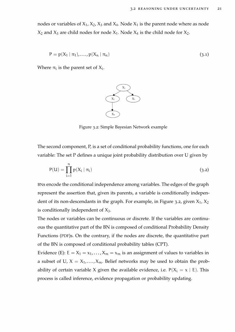
Figure 3.5: converging connection

are d-separated given B. thus evidence may be transmitted through a serial

connection unless the state of the variable in the connection is known (rule

1).

• Diverging connection. In Figure 3.4, inuence can pass between all the chil-

dren of A unless the state of A is known. It is said that B, C, ..., E are d-

separated given A. Thus evidence may be transmitted through a diverging

connection unless it is instantiated (rule 2).

• Converging connection. Figure 3.5 shows a converging connection. If noth-

ing is known about A except what may be inferred from knowledge of its

parents B, ..., E, then the parents is independent, i.e. evidence on one of them

has no influence on the certainty of the others. In other words, knowledge of

one possible cause of an event does not tell us anything about other possible

causes. However, if something is known about the consequences, then infor-

mation on one possible cause may tell us something about the other causes.

Thus evidence may only be transmitted through a converging connection if

either the variable in the connection or one of its descendants has received

evidence (rule 3).

Two distinct variables A and B in a causal network are d-separated if, for all paths

between A and B, there is an intermediate variable V such that either the connec-

tion is serial or diverging and V is instantiated, or the connection is converging,

and neither V nor any of V ’s descendants have received evidence. If A and B are

not d-separated, we call them d-connected.

3.3 bayesian networks 25

3.3.2 The chain rule and Bayes theorem for BNs

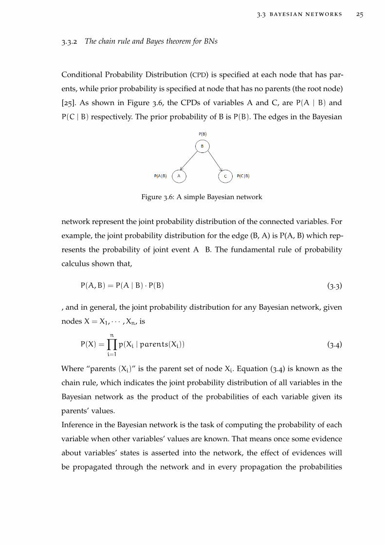
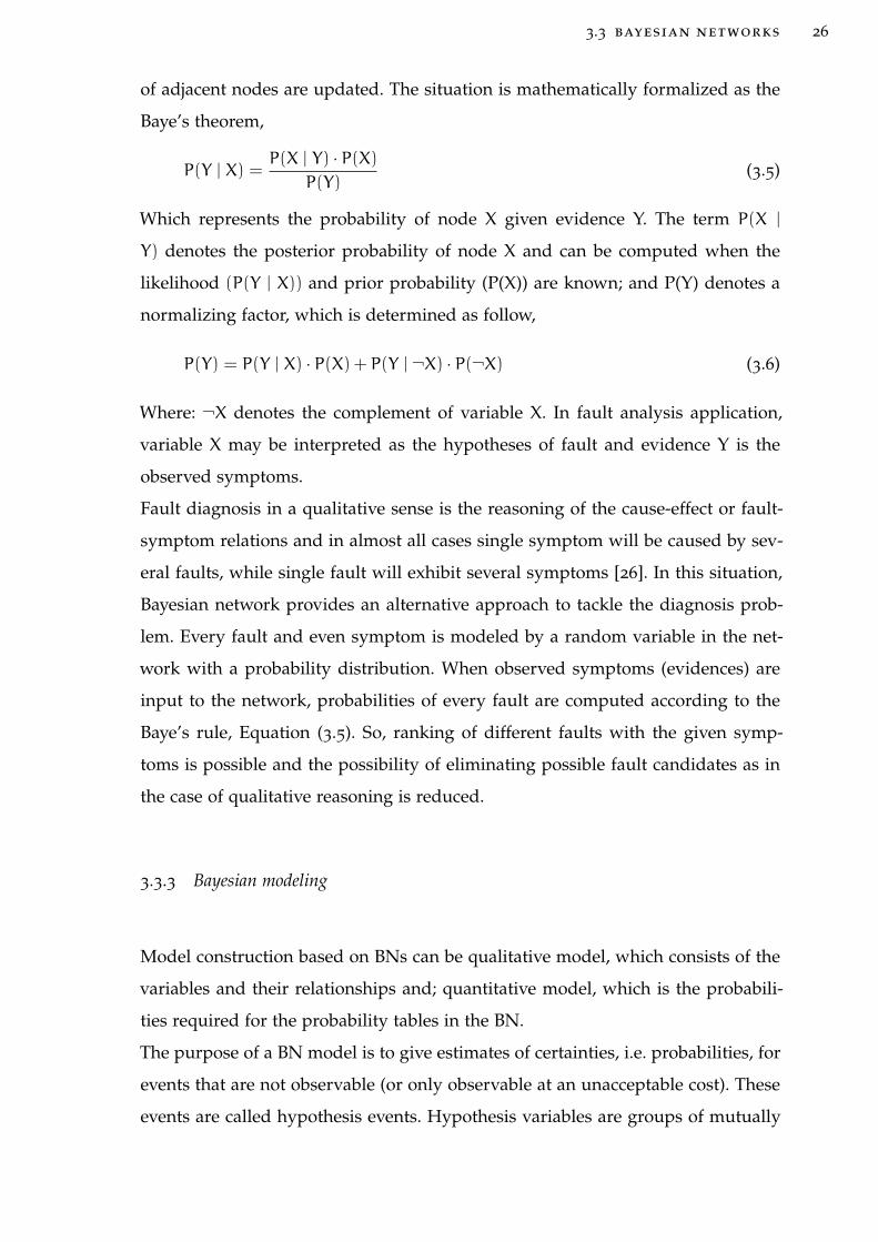
Conditional Probability Distribution (CPD) is specified at each node that has par-

ents, while prior probability is specified at node that has no parents (the root node)

[25]. As shown in Figure 3.6, the CPDs of variables A and C, are P(A | B) and

P(C | B) respectively. The prior probability of B is P(B). The edges in the Bayesian

Figure 3.6: A simple Bayesian network

network represent the joint probability distribution of the connected variables. For

example, the joint probability distribution for the edge (B, A) is P(A, B) which rep-

resents the probability of joint event A B. The fundamental rule of probability

calculus shown that,

P(A,B) = P(A | B) · P(B) (3.3)

, and in general, the joint probability distribution for any Bayesian network, given

nodes X = X1, · · · ,Xn, is

P(X) =

n∏i=1

p(Xi | parents(Xi)) (3.4)

Where “parents (Xi)” is the parent set of node Xi. Equation (3.4) is known as the

chain rule, which indicates the joint probability distribution of all variables in the

Bayesian network as the product of the probabilities of each variable given its

parents’ values.

Inference in the Bayesian network is the task of computing the probability of each

variable when other variables’ values are known. That means once some evidence

about variables’ states is asserted into the network, the effect of evidences will

be propagated through the network and in every propagation the probabilities

3.3 bayesian networks 26

of adjacent nodes are updated. The situation is mathematically formalized as the

Baye’s theorem,

P(Y | X) =P(X | Y) · P(X)

P(Y)(3.5)

Which represents the probability of node X given evidence Y. The term P(X |

Y) denotes the posterior probability of node X and can be computed when the

likelihood (P(Y | X)) and prior probability (P(X)) are known; and P(Y) denotes a

normalizing factor, which is determined as follow,

P(Y) = P(Y | X) · P(X) + P(Y | ¬X) · P(¬X) (3.6)

Where: ¬X denotes the complement of variable X. In fault analysis application,

variable X may be interpreted as the hypotheses of fault and evidence Y is the

observed symptoms.

Fault diagnosis in a qualitative sense is the reasoning of the cause-effect or fault-

symptom relations and in almost all cases single symptom will be caused by sev-

eral faults, while single fault will exhibit several symptoms [26]. In this situation,

Bayesian network provides an alternative approach to tackle the diagnosis prob-

lem. Every fault and even symptom is modeled by a random variable in the net-

work with a probability distribution. When observed symptoms (evidences) are

input to the network, probabilities of every fault are computed according to the

Baye’s rule, Equation (3.5). So, ranking of different faults with the given symp-

toms is possible and the possibility of eliminating possible fault candidates as in

the case of qualitative reasoning is reduced.

3.3.3 Bayesian modeling

Model construction based on BNs can be qualitative model, which consists of the

variables and their relationships and; quantitative model, which is the probabili-

ties required for the probability tables in the BN.

The purpose of a BN model is to give estimates of certainties, i.e. probabilities, for

events that are not observable (or only observable at an unacceptable cost). These

events are called hypothesis events. Hypothesis variables are groups of mutually

3.3 bayesian networks 27

exclusive events. To obtain a certainty estimate, there should be some information

channels which may reveal something about the hypothesis variables. These types

of information are grouped into information variables.

In our case, mobile site, there are twenty two variables. These are Indoor Unit

(IDU), Outdoor Unit (ODU), Antenna (Ant)1, Link1, Conf1, Link2, Aeronautical

Telecommunication Network (ATN), ODU, Microwave (MW), Optical (Opt), Transmission

(Tr), Alternating Current (AC), Diesel Generator (DG), Rect, Batt, Fuse, Conf2, Baseband

Unit (BBU), Remote Radio Unit (RRU), Ant2, MobileRF and NetworkOutage. Hav-

ing identified the variables for the model, the next step is establishing the directed

links. It is essential that the conditional independencies coded in the model cor-

respond with reality. The quantitative part of the model can be obtained from

dierent sources: subjective probabilities drew by experts, statistical data or theo-

retical considerations [27].

3.3.4 BN Learning

Learning is the process of building a BN based on previous training cases. When

we want to build a BN, we rely on two sources of information: input from domain

experts and statistical data [28]. Both the graph structure and the probability pa-

rameters are necessary to define a Bayesian network model. Even though some

experts can help to define the objectives and variables for a BN, the subjective sug-

gestions may not be accurate in sometimes. Expert’s experience combined with

historical data will make a model with better analytical and predicting ability.

Bayesian networks learning can be structure learning and parameters learning.

The parameter learning for Bayesian networks is the learning of the Conditional

Probability Table (CPT) [29]. The maximum likelihood estimates of the parameters

are easily leaned when the dataset is complete. When there are missing values in

the dataset, usually an Expectation Maximization (EM) algorithm is used to find

the maximum likelihood [30].

4A N A LY S I S O F B T S S I T E N E T W O R K O U TA G E

4.1 introduction

This chapter is devoted to the description of possible outage in cellular mobile net-

work is explained. In order to build analysis model the possible causes which may

give rise to the problem and their corresponding symptoms as well as the condi-

tioning parameters have to be identified. Analysis is carried out independently for

the site with problems. Therefore, it has been assumed that the diagnosis system

is utilized only on site with problems.

4.1.1 Basic definitions

A problem is defined as a situation in a site which has a degrading impact on the

service offered by that site [31]. Once the sites with problems are isolated, a root

cause of the problems should be done for each problematic elements of the site.

A cause or fault is the defective behavior of some logical or physical component

in the site that provokes failures and, finally, generates a problem. An example

of physical cause is a fault in one of the components in the site, whereas logical

cause example is link failure.

A symptom is a performance indicator or alarms whose value can be an indicator

of a fault, e.g. the power supply from the rectifier are malfunctioning.

A failure is an abnormal value of a symptom, which can be caused by a fault.

Therefore, a problem is a type of failure that has a negative influence on the ser-

vice offered to subscribers.

The knowledge base presented in this chapter is composed of the causes, symp-

4.2 causes of network outage 29

toms and conditions that frequently used for analysis. The information described

hereafter is based on interviews with domain experts and on my experience

and/or reading about radio access networks acquired during the development

of this thesis.

4.2 causes of network outage

There are various reasons for the network outages even there will not have a

single reason why an outage occurs; rather a sequence of events occur and leads

to site outage [32]. The trigger cause might be Transmission, Mobile RF, human

error, power loss, and natural disasters. These trigger causes; however, provide

little insight as to how the service outage has occurred. To understand the reason

why network outages occur requires root cause analysis.

For this thesis, only high level causes have been included into the diagnosis model.

The most common faults that may cause site outage are described in the following

sections.

4.2.1 Hardware

The diagram on Figure 2.1, shows the general hardware structure of BTS sites.

Meanwhile several modifications of the hardware have been made and many dif-

ferent versions exist especially for the RF-hardware parts. However, the general

principle can still be used for this analysis.

The base station modules are composed of elements that deteriorate over time,

some failing gradually and others suddenly. The effects of hardware faults can

lead to the site service outage. In most cases, when there is a hardware fault vari-

ous alarms are triggered.

The following points are some of the possible faults in the BTS hardware parts:

• Fault in one of the Transceivers (Transmitter/Receiver) (TRX)s (TRXn). The

transceivers (Transmitter /Receiver) or TRXs are the equipment that manage

4.2 causes of network outage 30

each of the carriers. The BTSs may have one or more TRXs. A TRX includes

a power amplifier for the downlink, a transmitter, a receiver and a baseband

unit (which is in charge of coding, interleaving, encryption and assembly in

bursts).

• Combiner fault. Combiners are used to connect various transmitters with

close frequencies to a single antenna. Isolation among transmitters is assured

and the signal from each of them is provide to the antenna with minimum

coupling.

• Antenna fault.

• Other faults in the RF transmission chain. It includes faults in the antenna

feeder, the connectors, the cables, etc.

• Other faults in the RF reception chain. The reception chain is composed of

diverse subsystems: duplexors, preselectors, antenna multicouplers, switch

matrices, etc.

• Other HW faults. Besides the previous elements, base stations include other

subsystems, such as synchronization circuits, power supply; A-bis interface

connection, air conditioning, etc. Any of these might be the cause of site

outage.

4.2.2 Transmission

In telecommunications, transmission (abbreviations: Tx) is the process of sending

and propagating an analogue or digital information signal over a physical point-

to-point or point-to-multipoint transmission medium, either wired, optical fiber

or wireless.

Network outage due to Transmission, causes have been divided into two sub

causes: Microwave failure and Optical failure.

Microwave failure includes IDU, ODU, Ant, Link and configuration failures. Optical

failure includes ODU, ATN and link failure.

4.2 causes of network outage 31

4.2.3 Power system failure

First, suppose commercial AC power failed. Although the generator operated

properly, the rectifiers were damaged by the commercial AC failure. Once the

rectifier failed, no DC power could be generated, even though the generator was

working properly. The batteries supplied the required DC voltage levels until they

were depleted and the telecom equipment shut down. Let us see a few possible

outage cause of power system failure in different cases.

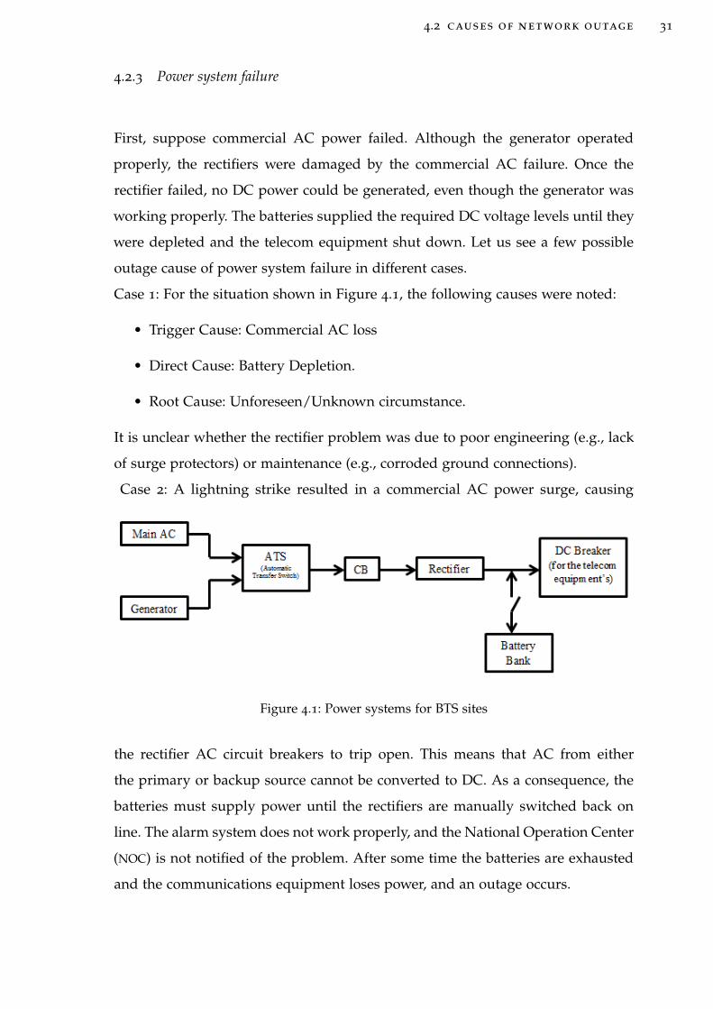
Case 1: For the situation shown in Figure 4.1, the following causes were noted:

• Trigger Cause: Commercial AC loss

• Direct Cause: Battery Depletion.

• Root Cause: Unforeseen/Unknown circumstance.

It is unclear whether the rectifier problem was due to poor engineering (e.g., lack

of surge protectors) or maintenance (e.g., corroded ground connections).

Case 2: A lightning strike resulted in a commercial AC power surge, causing

Figure 4.1: Power systems for BTS sites

the rectifier AC circuit breakers to trip open. This means that AC from either

the primary or backup source cannot be converted to DC. As a consequence, the

batteries must supply power until the rectifiers are manually switched back on

line. The alarm system does not work properly, and the National Operation Center

(NOC) is not notified of the problem. After some time the batteries are exhausted

and the communications equipment loses power, and an outage occurs.

4.2 causes of network outage 32

• Trigger Cause: Lightning strike.

• Direct Cause: Battery Depletion.

• Root Cause: Maintenance - failure to test alarms.

Case 3: A wrench dropped by a maintenance worker landed on an exposed DC

power bus which shorted out. Exposed power buses should be covered before

maintenance activity starts. Maintenance personnel error can be reduced by pro-

viding sufficient training to personnel.

• Trigger Cause: Dropping a tool.

• Direct Cause: DC short circuit.

• Root Cause: Human error – maintenance

As seen from these cases, outage summaries must be studied to identify trigger,

direct, and root causes. This analysis provides a better understanding of why the

outage has occurred and what can be done to prevent like occurrences.

4.2.4 Other failures

There are other faults which are not included in the ones explained in the previ-

ous sections, which occur rarely. These are bad adjacency definition and erroneous

configuration parameters. In the RAN there are thousands of configuration param-

eters per BTS, which should be updated when the network evolves. If any of the

important parameters is incorrect, failure may appear.

The climate may have an impact on the faults occurring in the cells. For example,

in moist climates where rain is frequent, the probability of hardware faults in-

creases. This is due to the fact that water can easily get into a piece of equipment

or some connections may become lose. The configuration denoted as “Climate”

may take on the values wet, normal or dry.

Antenna alignment has a direct impact on the network performance or even out-

age. If the antenna is misaligned dropped calls may happen and eventually site

outage.

4.2 causes of network outage 33

Another configuration parameter is the “antenna tilt”. If the antenna is down tilted

too much, service will degrade may show up because of lack of coverage in the

border areas. If the tilt is not enough, site outage may appear in the serving site.

5C A S E S T U D Y

Here is a case study on the analysis of ethio telecom (ET) BTS site network outage

using Bayesian networks.

Two approaches with different failure probability distributions are discussed. A

brief methodology used in fault tree analysis is used. Bayesian networks with two

state nodes are applied. A research on the application of Bayesian networks in

the continuous system is not covered due to its applicability in mobile network

outage analysis.

5.1 system introduction

Cellular mobile networks consist of different hardware elements: switching units,

cables, cooling elements, energy elements, etc. Many of the possible relations be-

tween elements are not explicitly defined. For example, the typical case is a fibber

cut-off that makes many dependent mobile base stations be in turn cut off, con-

sequently affecting many customers. While in certain types of hardware elements

this information is explicitly modeled, it is not the case in many others. This makes

it difficult to use traditional programming solutions to automatically link failures

to a root cause incident management systems, usually known as TT systems, of-

fer the technician the possibility to link an incident produced on an element to

another existing incident, creating a child-parent relation. The existing elements

found in the mobile sites are as shown in Figure 2.1.

In this case study, a Bayesian networks methodology combined with fault tree

analysis is used for the root cause analysis of mobile site outage in discrete failure

distribution. First work on fault tree analysis then converts it to Bayesian analysis

approach.

5.2 discrete failure distribution 35

5.2 discrete failure distribution

Suppose all the failure rate of the components in the BTS network is assumed con-

stant. A reduced fault tree analysis approach and Bayesian network approach with

multiple states are built to better facilitate the implementation and understanding.

5.2.1 Fault Tree Analysis Approach

Fault Tree Analysis (FTA) is a very popular and diffused technique for the de-

pendability modeling and evaluation of large, safety-critical systems [33]. The

technique is based on the identification of a particular undesired event to be ana-

lyzed (e.g. system failure), called the Top Event (TE). The construction of the Fault

Tree (FT) proceeds in a top to down fashion, from the events to their causes, un-

til failures of basic components are reached. The methodology assumes events are

binary events (working/not-working); events are statistically independent; and re-

lationships between events and causes are represented by means of logical AND

and OR gates.

Taking the cellular network site outage as the top event, analyzing from the top to

down and step by step, we can get the following fault tree shown in Figure 5.1.

The top event, Network_Outage, with an OR gate connects with event, Transmis-

sion and Mobile_RF, which presents the mobile network system failure. And event

Transmission, with an AND gate connects with event microwave (MW) and opti-

cal (opt) network failures. The MW event also an OR gate with IDU, ODU, Ant1,

Link1, conf1 and Fuse. Any one of the six events down can lead to event MW

failure happen. On the other hand the optical event an OR gate with Link2, ATN,

ODF and Fuse. Also one of the four down can lead to event optical failure happen.

Event Mobile_RF with an OR gate connects with events conf2, BBU, RRU, Ant2

and Fuse. Any one of the five down can lead to event Mobile_RF happen.

For the power supply system which will supply power to the BTS equipment’s

through Fuse is connected by OR gate with MW, Opt and Mobile_RF. And event

Fuse AND gate with Rectifier (Rect) and Battery (Batt). Also the rectifier event

5.2 discrete failure distribution 36

with an AND gate connects with event commercial power (AC) and generator

(DG). So for the Fuse failure to happen, both event Rect and Battery failure should

occur, also for the Rect failure both AC and DG should down. Parent nodes param-

eter definition for this fault tree is shown in the Appendix part Table A.1. There

Figure 5.1: Fault Tree Structure for BTS Network

are three AND gates and four OR gates in the fault tree diagram.

5.2.2 Bayesian Network Approach

For the above fault tree (FT), it is straightforward to map it into a BN, i.e. a BN

with every variable/nodes having two acceptable values: event happens (=1) or

not happened (=2). For the sake of simplicity, let us for now consider FT having

just AND/OR gates: the mapping can be obtained as follows [34]:

5.2 discrete failure distribution 37

• For each leaf node (i.e. basic system component) of the FT, create a root node

in the BN having the same (prior) probability distribution as in the FT;

• For each gate of the FT, create a corresponding node in the BN;

• Label the node corresponding to the gate whose output is the system failure

of the FT as the Fault node;

• Connects nodes in the BN as corresponding gates are connected in the FT;

• For each node corresponding to an AND (respectively OR) gate create a CPT

such that the node is true with probability 1 if and only if all incoming nodes

are true (respectively if and only if at least one incoming node is true) while

it is false with probability 1 elsewhere.

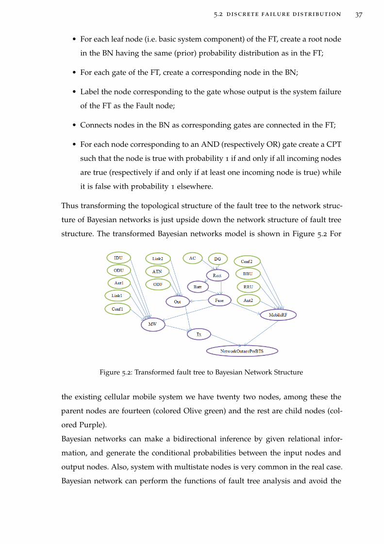
Thus transforming the topological structure of the fault tree to the network struc-

ture of Bayesian networks is just upside down the network structure of fault tree

structure. The transformed Bayesian networks model is shown in Figure 5.2 For

Figure 5.2: Transformed fault tree to Bayesian Network Structure

the existing cellular mobile system we have twenty two nodes, among these the

parent nodes are fourteen (colored Olive green) and the rest are child nodes (col-

ored Purple).

Bayesian networks can make a bidirectional inference by given relational infor-

mation, and generate the conditional probabilities between the input nodes and

output nodes. Also, system with multistate nodes is very common in the real case.

Bayesian network can perform the functions of fault tree analysis and avoid the

5.2 discrete failure distribution 38

limitation of fault tree analysis, i.e., one of the limitations of fault tree analysis is

that all the events can only have binary states. However Bayesian networks can

assume that components have more than two states. For each root nodes which is

also called parent nodes, there is a Marginal Probability Distribution (MPD). This

will present all the possible states of the node and their probabilities value which

may be from data, TT, or expertise thought. For every other node in the Bayesian

network, a Conditional CPD is used to describe its probability distribution given

the states of the parent nodes.

When a node is equal to 1, then it means this node fails or event happen; when it

is equal to 2, then this part of the system is still functional or events not happen.

It is possible to define the relationship between components, for example, node

MW, Opt, Rect, Batt, Fuse, Tr, MobileRF and NetworkoutageperBTS and calculate

their CPDs. However it’s difficult to describe some complex relationships of the

nodes/elements/variables with fault tree approach/gate.

The BN represents the joint probability distribution P(IDU, ODU, Ant1, Link1,

Conf1, Link2, ATN, ODF, MW, Opt, Tr, AC, DG, Rect, Batt, Fuse, Conf2, BBU,

RRU, Ant2, MobileRF, NetworkOutage). A particular value in the joint distribu-

tion is P(idu, odu, ant1, link1, conf1, link2, atn, odf, mw, opt, tr, ac, dg, rect, batt,

fuse, conf2, bbu, rru, ant2, mobilerf, networkoutage).

Applying the chain rule for the BTS site’s node, can get the factorization as:

P(idu, odu, ant1, link1, conf1, link2, atn, odf, mw, opt, tr, ac, dg, rect, batt, fuse,

conf2, bbu, rru, ant2, mobilerf, networkoutage) = [p(idu) ·p(odu) ·p(ant1) ·p(link1) ·

p(conf1) · p(link2) · p(atn) · p(odf) · p(mw | (idu,odu,ant1, link1, conf1, fuse)) ·

p(opt | (link2,atn,odf)) · p(tr | (mw,opt)) · p(ac) · p(dg) · p(rect | (ac,dg)) ·

p(batt | rect) ·p(fuse | (rect,Batt)) ·p(conf2) ·p(bbu) ·p(rru) ·p(ant2) ·p(mobilerf |

(conf2,bbu, rru,ant2, fuse)) · p(networkoutage | Tr,mobilerf)]

6B AY E S I A N N E T W O R K M O D E L A N D A N A LY S I S R E S U LT S

6.1 model based on bayesian networks

To build the Bayesian network model for the mobile network system, a Bayes Net

Toolbox for Matlab is introduced in this paper [35]. This Matlab toolkit allows

creating Bayesian networks, either manually or by learning; doing some BNs infer-

ence like computing marginal distribution and joint distribution; conduct learning

for the BNs by estimating from given dataset, and applying algorithms like struc-

tural EM; it can also use some inference engines like junction tree.

The main functions used from the toolkit are manually creating the Bayesian net-

work graph shell and imputing conditional probability distribution, and BNs in-

ference computing.

The graph structure from Matlab is shown in Figure 6.1, which is the same as

what we designed in Figure 5.2.

One of the most important advantages of Bayesian networks is when given any

evidence; it can calculate the conditional probability between the input nodes and

the output nodes, and conduct a more accurate probability inference. The condi-

tional probability will give valuable suggestions for the system reliability analysis,

failure diagnosis and system maintenance plan. Besides, the capability of ana-

lyzing multistate failure distribution avoids a significant limitation of fault tree

approach, which gives a better representation of the real system.

Now given the evidence that the network outage happens, which means Nout=1

and network is working properly, i.e., Nout=2 (failure not happen), the conditional

probability for each component, for example IDU, ODU, Link1, Ant1 and Conf1

nodes, is calculated by using Matlab and shows in the following Table 3. The in-

ference engine used in the case study is junction tree engine.

6.1 model based on bayesian networks 40

Figure 6.1: Generated Bayesian Networks Structure

Since Bayesian network has a bi-directional inference feature, so the reverse pro-

Table 6.1: Conditional probability distribution for the five components

xi IDU ODU Link1 Ant1 Conf1

P(i=1|NetworkOutagePerBTS=1) 0.4772 0.2527 0.1471 0.0938 0.162

P(i=1|NetworkOutagePerBTS=2) 0.5228 0.7473 0.8529 0.9062 0.838

cess i.e., the CPD of IDU, ODU, Ant1, Link1 and Conf1 given network outage

happen is as shown in Figure 6.2.

Now let us do for the parent nodes given network outage is happen. Assign num-

ber for all nodes as IDU=1, ODU=2, Ant1=3, Link1=4, Conf1=5, Link2=6, ATN=7,

ODF=8, MW=9, Opt=10, Tr=11, AC=12, DG=13, Rect=14, Batt=15, Fuse=16, Conf2=17,

BBU=18, RRU=19, Ant2=20, MobileRF=21 and NetworkOutage=22.

The following Figure 6.3 compares the influences of each parent component fail-

ure on the system failure. This indicates that node 1, 6, 12 and 17 has a significant

influence for the root causes of network outage. So these nodes have the high-

est CPD among all parent node components in the network outage system. And

also node 2, 7, 13 and 18 has also influence for the root causes of network outage

whereas the rest would have moderate influence of network outage. To strengthen

6.1 model based on bayesian networks 41

Figure 6.2: Conditional probability of IDU, ODU, Ant1, Link1 and conf1 given Nout=1

the network reliability, more effort should be done to ensure a low failure rate for

the system.

For the bidirectional inference, when calculating the CPD of Network outage given

all parent nodes fail(=1) are the failure rate value each parent nodes itself i.e.,

P(network Outage=1|parentNode)=1.

The horizontal axis represent the fourteen parent nodes where as the vertical axis

Figure 6.3: Conditional probability of parent nodes given Nout=1

represents the probability of failure for the nodes.

Current research on Bayesian networks are mainly concerned about two aspects:

Bayesian networks learning and Bayesian networks inference.

6.2 bayesian networks learning 42

6.2 bayesian networks learning

When we want to build a BN, we rely on two sources of information: input from

domain experts and statistical data [8]. Both the graph structure and the proba-

bility parameters are necessary to define a Bayesian network model. Even though

some experts can help to define the objectives and variables for a BN, the subjec-

tive suggestions may not be accurate in some times. Expert’s experience combined

with historical data will make a model with better analytical and predicting abil-

ity.

Bayesian networks learning can be structure learning and parameters learning.

Structure learning for Bayesian networks is the learning of the interconnection of

nodes/variables in the graph; whereas parameter learning is the learning of the

CPT of the variables. The maximum likelihood estimates of the parameters are

easily leaned when the dataset is complete. When there are missing values in the

dataset, usually an EM algorithm is used to find the maximum likelihood. The tool

used for learning and inference is Matlab.

Bayesian learning means computing a posterior over the parameters given fully

observed data.

Bayes Rule:

P(x | y) =P(y | x) · P(x)

P(y)(6.1)

Where:

P(x | y) – Posterior distribution, informs which parameters are likely given the

observed data.

P(x) - Prior distribution, represents any knowledge we have about how the data

generated prior to observing them.

P(y) - Observed data (Network outage)

P(y | x) - likelihood function for the data.

6.2 bayesian networks learning 43

6.2.1 Code / BNT class structure

A CPD defines P(X(i)|X(Pa(i))), where X(i) is the i’th node, and X(Pa(i)) are the

parents of node i. There are many ways to represent this distribution, which de-

pend in part on whether X(i) and X(Pa(i)) are discrete, continuous, or a combina-

tion. Only discrete variables are considered. If the CPD is represented as a table

(i.e., if it is a multinomial distribution), it has a number of parameters that is

exponential in the number of parents. List of all the different types of CPDs sup-

ported by BNT are: Noisy-or nodes, Other (noisy) deterministic nodes, Softmax

(multinomial logit) nodes, Neural network nodes, Root nodes, Gaussian nodes,

Generalized linear model nodes and Classification/regression tree nodes.

The model used for Bayesian Network Toolbox (BNT) class structure is “bnet” for

thesis work. Also the CPD use Gaussian, tabular, softmax, root. For inference

engine, both, exact and approximate, are used as necessary. For exact inference-

junction tree and for approximate- sampling. For learning engine only parameter

learning is applied, like: EM. You can see each BNT class structure in the code part,

Appendix I.

6.2.2 Parameter learning

Loading data from an American Standard Code for Information Interchange (ASCII)

text file called ’data.txt’, where each row is a case and columns are separated by

white-space. The file is written in the matlab as “load data.txt –ascii”.

BNT learning routines require data to be stored in a cell array. datai,m is the value

of node i in case m, i.e., each column is a case. If node i is not observed in case m

(missing value), set datai,m = [].

Loading leveled TT dataset:

As can be seen from Figure 6.4, it can successfully train the fault distribution of

BTS site. The horizontal line is the number of cases where as the vertical line is

their probability value. Create a training sample network with random parameters

using forward sampling from the previously creating bnet. Create some training

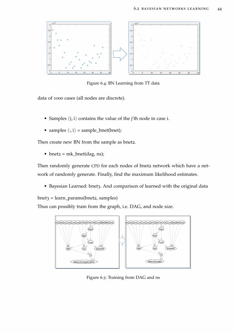
6.2 bayesian networks learning 44

Figure 6.4: BN Learning from TT data

data of 1000 cases (all nodes are discrete).

• Samples (j, i) contains the value of the j’th node in case i.

• samples (:, i) = sample_bnet(bnet);

Then create new BN from the sample as bnet2.

• bnet2 = mk_bnet(dag, ns);

Then randomly generate CPD for each nodes of bnet2 network which have a net-

work of randomly generate. Finally, find the maximum likelihood estimates.

• Bayesian Learned: bnet3. And comparison of learned with the original data

bnet3 = learn_params(bnet2, samples)

Thus can possibly train from the graph, i.e. DAG, and node size.

Figure 6.5: Training from DAG and ns

7C O N C L U S I O N A N D R E C O M M E N D AT I O N

7.1 conclusion

In the ethio telecom case study, the thesis considered and developed a BTS mo-

bile network system. The possible relations between elements are explicitly well-

defined and there are twenty two nodes or variables and try to link failures to a

root cause incident management systems, also known TT systems, which provides

a clue to the technician the possibility to link an incident produced on an element

to another existing incident, creating a child-parent relation. So, it depends on

expert knowledge to be able to identify these situations quickly. Two approached

used to model the BTS site and a brief methodology used in fault tree and Bayesian

networks. The transforming of the topological structure of the fault tree to the net-

work structure of Bayesian networks is just upside down the network structure of

fault tree structure.

In Bayesian networks, when given any evidence; it can calculate the conditional

probability between the input nodes and the output nodes, and conduct a more

accurate probability inference. Given the evidence that the network outage hap-

pens, which means Nout=1 and network is working properly, i.e., Nout=2 (failure

not happen), the conditional probability for each component, for example IDU,

ODU, Link1, Ant1 and Conf1 nodes, can be calculated by using Matlab. It’s also

work for the bidirectional inference, when calculating the CPD of Network outage

given all parent nodes fail(=1) are the failure rate value each parent nodes itself

i.e., P(network Outage=1|parentNode)=1.

The main motivation of this thesis work is to investigate the BTS site network out-

7.2 recommendation 46

age in a case of ethio telecom. The investigation is made by analyzing collected

real TT data. Based on the analysis result and literature review, model based ap-

proach for investigating the root causes of failure is proposed.

The main challenges noticed in doing this thesis is that the exported TT data avail-

ability in the NOC are not as such good enough to leveling the raw data especially

a challenge in the learning process. On the other hand the subjectivity concepts of

the model that should work on the expertise are not always true.

7.2 recommendation

Here are some of the points recommended as a future work that might continue

the thesis work :

• More trials in live networks would be helpful to strengthen the practical

conclusions of this thesis.

• The logical continuation of the performed investigation that is the applica-

tion of techniques proposed in this thesis to other network technologies, such

as fixed networks or other.

R E F E R E N C E S

[1] E. Rozaki, “Design and implementation for automated network troubleshoot-

ing using data mining,” arXiv preprint arXiv:1506.00108, 2015.

[2] L. Lewis, “A case-based reasoning approach to the management of faults

in communication networks,” in INFOCOM’93. Proceedings. Twelfth Annual

Joint Conference of the IEEE Computer and Communications Societies. Networking:

Foundation for the Future, IEEE, IEEE, 1993, pp. 1422–1429.

[3] bill wilson. (Mar. 6, 2017). Root cause analysis. [Online; 2017-03-06], [Online].

Available: https://www.bill-wilson.net/root-cause-analysis.

[4] R. Sasisekharan, V Seshadri, and S. M. Weiss, “Data mining and forecast-

ing in large-scale telecommunication networks,” IEEE Expert, vol. 11, no. 1,

pp. 37–43, 1996.

[5] Y. Temprado, F. J. Molinero, C. Garcia, and J. Gomez, “Knowledge discov-

ery from trouble ticketing reports in a large telecommunication company,”

in Computational Intelligence for Modelling Control & Automation, 2008 Interna-

tional Conference on, IEEE, 2008, pp. 37–42.

[6] K. B. Korb and A. E. Nicholson, Bayesian artificial intelligence. CRC press,

2010.

[7] D. Koller, N. Friedman, and F. Bach, Probabilistic graphical models: principles

and techniques. MIT press, 2009.

[8] F. J. M. Velasco, “A bayesian network approach to diagnosing the root cause

of failure from trouble tickets,” Artificial Intelligence Research, vol. 1, no. 2,

p. 75, 2012.

[9] ethio telecom. (Dec. 22, 2017). Ethio telecom ranked first in africa. [Online;

2017-12-22], [Online]. Available: http : / / www . ethiotelecom . et / press -

release.

references 48

[10] cision PR Newswire. (Dec. 22, 2017). Ethio telecom ranked first in africa. [On-

line; 2017-12-22], [Online]. Available: https://www.prnewswire.com/news-

releases/ethiopia---telecoms-mobile-and-broadband---statistics-

and-analyses-300552315.html.

[11] ethio telecom, “Performance report of ethio telecom,” Dec. 6, 2016, [Online;

2017-10-12]. [Online]. Available: http://www.ethiotelecom.et/.

[12] I. Katzela and M. Schwartz, “Schemes for fault identification in communi-

cation networks,” IEEE/ACM Transactions on Networking (TON), vol. 3, no. 6,

pp. 753–764, 1995.

[13] M. Steinder and A. S. Sethi, “Probabilistic fault localization in communica-

tion systems using belief networks,” IEEE/ACM Transactions on Networking

(TON), vol. 12, no. 5, pp. 809–822, 2004.

[14] L. Lewis and G. Dreo, “Extending trouble ticket systems to fault diagnos-

tics,” IEEE network, vol. 7, no. 6, pp. 44–51, 1993.

[15] L. Abele, M. Anic, T. Gutmann, J. Folmer, M. Kleinsteuber, and B. Vogel-

Heuser, “Combining knowledge modeling and machine learning for alarm

root cause analysis,” IFAC Proceedings Volumes, vol. 46, no. 9, pp. 1843–1848,

2013.

[16] M. W. Browne, “Cross-validation methods,” Journal of mathematical psychol-

ogy, vol. 44, no. 1, pp. 108–132, 2000.

[17] Techopedia. (Sep. 12, 2018). Cellular network. [Online; 2018-09-12], [Online].

Available: https://www.techopedia.com/definition/24962/cellular-

network.

[18] C. Nuangjamnong, S. P. Maj, and D. Veal, “The osi network management

model-capacity and performance management,” 2008.

[19] C. Bettstetter, F. Fitzek, H Hartenstein, G Pujolle, and P Santi, “Special issue

on self-organisation in mobile networking,” European Transactions on Telecom-

munications, vol. 16, no. 5, pp. 371–373, 2005.

[20] C. Melchiors and L. M. R. Tarouco, “Troubleshooting network faults using

past experience,” in Network Operations and Management Symposium, 2000.

NOMS 2000. 2000 IEEE/IFIP, IEEE, 2000, pp. 549–562.

references 49

[21] G. Vorley, “Mini guide to root cause analysis,” Quality Management and Train-

ing, London, 2008.

[22] D. Hayward. (May 6, 2014). The 4 building blocks of root cause analysis.

[Online; 2017-10-12], [Online]. Available: http://www.apmdigest.com/the-

4-building-blocks-of-root-cause-analysis.

[23] F. V. Jensen and T. Nielsen, “Bayesian networks and decision graphs springer-

verlag,” New york, 2001.

[24] M. Lindberg, Decision support systems: Diagnostics and explanation methods: In

the context of telecommunication networks, 2013.

[25] C. Lo, Y. Wong, and A. Rad, “Bayesian network for fault diagnosis,” in Eu-

ropean Control Conference (ECC), 2003, IEEE, 2003, pp. 1381–1386.

[26] H. Kirsch and K. Kroschel, “Applying bayesian networks to fault diagnosis,”

in Proceedings of the Third IEEE Conference on Control Applications, vol. 2, 1994,

pp. 895–900.

[27] C. Skaanning, F Jensen, U. Kjærulff, and A Madsen, “Acquisition and trans-

formation of likelihoods to conditional probabilities for bayesian networks,”

in Proc. AAAI Spring Symposium on AI in Equipment Maintenance Service and

Support, Palo Alto, California, 1999, p. 3440.

[28] H. Langseth and L. Portinale, “Bayesian networks in reliability,” Reliability

Engineering & System Safety, vol. 92, no. 1, pp. 92–108, 2007.

[29] P. M. Lee, Bayesian statistics: an introduction. John Wiley & Sons, 2012.

[30] A. P. Dempster, N. M. Laird, and D. B. Rubin, “Maximum likelihood from

incomplete data via the em algorithm,” Journal of the royal statistical society.

Series B (methodological), pp. 1–38, 1977.

[31] J. Laiho, M. Kylvaja, and A. Hoglund, “Utilization of advanced analysis

methods in umts networks,” in Vehicular Technology Conference, 2002. VTC

Spring 2002. IEEE 55th, IEEE, vol. 2, 2002, pp. 726–730.

[32] R. Barco-Moreno et al., “Bayesian modelling of fault diagnosis in mobile

communication networks,” 2007.

references 50

[33] A. Bobbio, L. Portinale, M. Minichino, and E. Ciancamerla, “Comparing

fault trees and bayesian networks for dependability analysis,” in Interna-

tional Conference on Computer Safety, Reliability, and Security, Springer, 1999,

pp. 310–322.

[34] M. Malhotra and K. S. Trivedi, “Dependability modeling using petri-nets,”

IEEE Transactions on reliability, vol. 44, no. 3, pp. 428–440, 1995.

[35] murphyk. (Nov. 13, 2002). How to use the bayes net toolbox. [Online; 2018-

08-17], [Online]. Available: https://www.cs.ubc.ca/~murphyk/Software/

BNT/usage_02nov13.html.

AA P P E N D I X - I

TT Data leveling and knowledge bases assumptions

This appendix-I presents the methods and models proposed in this thesis, Bayesian

Network.

When we build BN, we need to have:

• expert knowledge,

• system designs, and

• Learned from data.

Steps for specifying a BN:

• Define the variables and their values

• Define the structure

• Define the CPTs, parameters

System Model

Existing elements found in the mobile sites that are represented in the model are

as shown in the Figure A.1. Parent nodes parameter definition for this fault tree

is shown in Table A.1.

Table A.1: Parent nodes definition

Par. Event Event Description

1 IDU In-Door Unit: to receive and decode satellite transmissions

Continued on next page

appendix-i 52

Table A.1 – continued from previous page

Par. Event Event Description

2 ODU Outdoor Unit: The term ODU is used in Split-Mount Microwave

systems where an Indoor Unit (IDU) is typically mounted in an

indoor location connected via a coaxial cable to the ODU which is

mounted on a rooftop or tower top location.

3 Ant1 Antennas are bridging the gap between electronic and electromag-

netic signals. The antenna’s length, for example, corresponds to the

length of the radio waves the antenna receives or transmits.

4 Link1 Link is generally one of several types of information transmission

paths such as those provided by communication satellites, terrestrial

radio communications infrastructure

5 Conf1 Network configuration is the process of setting a network’s controls,

flow and operation to support the network communication of an

organization and/or network owner.

6 Link2 Link is generally one of several types of information transmission

paths such as those provided by communication satellites, terres-

trial radio communications infrastructure and computer networks

to connect two or more points.

7 ATN Aeronautical Telecommunication Network (ATN) is an internet-

work architecture that allows ground/ground, air/ground, and

avionic data sub networks to interoperate by adopting common

interface services and protocols based on the ISO OSI Reference

Model.

8 ODF Optical distribution frame (ODF) is a frame used to provide cable

interconnections between communication facilities, which can inte-

grate fiber splicing, fiber termination, fiber optic adapters & connec-

tors and cable connections together in a single unit.

Continued on next page

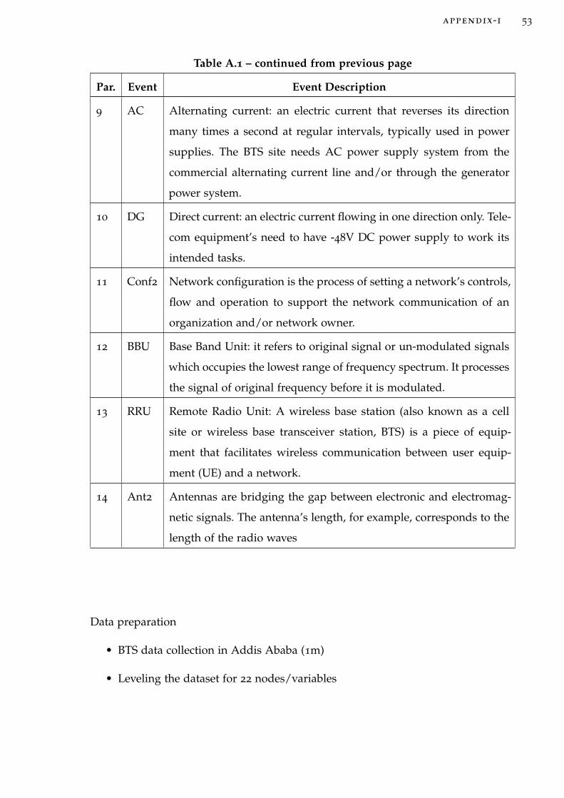
appendix-i 53

Table A.1 – continued from previous page

Par. Event Event Description

9 AC Alternating current: an electric current that reverses its direction

many times a second at regular intervals, typically used in power

supplies. The BTS site needs AC power supply system from the

commercial alternating current line and/or through the generator

power system.

10 DG Direct current: an electric current flowing in one direction only. Tele-

com equipment’s need to have -48V DC power supply to work its

intended tasks.

11 Conf2 Network configuration is the process of setting a network’s controls,

flow and operation to support the network communication of an

organization and/or network owner.

12 BBU Base Band Unit: it refers to original signal or un-modulated signals

which occupies the lowest range of frequency spectrum. It processes

the signal of original frequency before it is modulated.

13 RRU Remote Radio Unit: A wireless base station (also known as a cell

site or wireless base transceiver station, BTS) is a piece of equip-

ment that facilitates wireless communication between user equip-

ment (UE) and a network.

14 Ant2 Antennas are bridging the gap between electronic and electromag-

netic signals. The antenna’s length, for example, corresponds to the

length of the radio waves

Data preparation

• BTS data collection in Addis Ababa (1m)

• Leveling the dataset for 22 nodes/variables

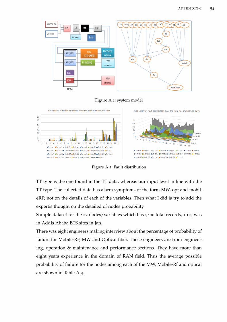
appendix-i 54

Figure A.1: system model

Figure A.2: Fault distribution

TT type is the one found in the TT data, whereas our input level in line with the

TT type. The collected data has alarm symptoms of the form MW, opt and mobil-

eRF; not on the details of each of the variables. Then what I did is try to add the

expertis thought on the detailed of nodes probability.

Sample dataset for the 22 nodes/variables which has 5400 total records, 1015 was

in Addis Ababa BTS sites in Jan.

There was eight engineers making interview about the percentage of probability of

failure for Mobile-RF, MW and Optical fiber. Those engineers are from engineer-

ing, operation & maintenance and performance sections. They have more than

eight years experience in the domain of RAN field. Thus the average possible

probability of failure for the nodes among each of the MW, Mobile-Rf and optical

are shown in Table A.3.

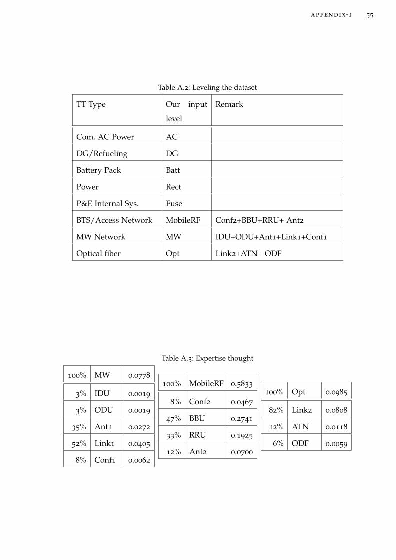
appendix-i 55

Table A.2: Leveling the dataset

TT Type Our input

level

Remark

Com. AC Power AC

DG/Refueling DG

Battery Pack Batt

Power Rect

P&E Internal Sys. Fuse

BTS/Access Network MobileRF Conf2+BBU+RRU+ Ant2

MW Network MW IDU+ODU+Ant1+Link1+Conf1

Optical fiber Opt Link2+ATN+ ODF

Table A.3: Expertise thought

100% MW 0.0778

3% IDU 0.0019

3% ODU 0.0019

35% Ant1 0.0272

52% Link1 0.0405

8% Conf1 0.0062

100% MobileRF 0.5833

8% Conf2 0.0467

47% BBU 0.2741

33% RRU 0.1925

12% Ant2 0.0700

100% Opt 0.0985

82% Link2 0.0808

12% ATN 0.0118

6% ODF 0.0059

appendix-i 56

The raw data input to the matlab for learning. Row are days and columns are

number of variables as shown Figure A.3.

Figure A.3: leveled dataset