Full Terms & Conditions of access and use can be found athttp://www.tandfonline.com/action/journalInformation?journalCode=upri20

Download by: [Virginia Tech Libraries] Date: 09 November 2016, At: 13:46

PRIMUSProblems, Resources, and Issues in Mathematics UndergraduateStudies

ISSN: 1051-1970 (Print) 1935-4053 (Online) Journal homepage: http://www.tandfonline.com/loi/upri20

Roots of Linear Algebra: An Historical Explorationof Linear Systems

Christine Andrews-Larson

To cite this article: Christine Andrews-Larson (2015) Roots of Linear Algebra: An HistoricalExploration of Linear Systems, PRIMUS, 25:6, 507-528, DOI: 10.1080/10511970.2015.1027975

To link to this article: http://dx.doi.org/10.1080/10511970.2015.1027975

Accepted author version posted online: 01Apr 2015.Published online: 01 Apr 2015.

Submit your article to this journal

Article views: 393

View related articles

View Crossmark data

PRIMUS, 25(6): 507–528, 2015Copyright © Taylor & Francis Group, LLCISSN: 1051-1970 print / 1935-4053 onlineDOI: 10.1080/10511970.2015.1027975

Roots of Linear Algebra: An Historical Explorationof Linear Systems

Christine Andrews-Larson

Abstract: There is a long-standing tradition in mathematics education to look to his-tory to inform instruction. An historical analysis of the genesis of a mathematical ideaoffers insight into: (i) the contexts that give rise to a need for a mathematical construct;(ii) the ways in which available tools might shape the development of that mathemati-cal idea; and (iii) ways in which students might make sense of an idea. In this paper, Idiscuss historic contexts that gave rise to considerations of linear systems of equationsand their solutions, as well as implications for instruction and instructional design.

Keywords: Systems of linear equations, linear algebra, history.

1. INTRODUCTION

History provides a wealth of resources with the potential to inform the teach-ing and learning of mathematics [2,6,22]. Instructional insights can be gleanedfrom history by considering the contexts that gave rise to a need for a mathe-matical idea, the ways in which available tools might shape the development ofthat idea, and the ways in which students might make sense of that idea. Suchinsights can be particularly important for instruction and instructional designin inquiry-oriented approaches where students are expected to reinvent signifi-cant mathematical ideas. Sensitivity to the original contexts and notations thatafforded the development of particular mathematical ideas is invaluable to theinstructor or instructional designer who aims to facilitate students’ reinventionof such ideas. This article explores the ways in which instruction and instruc-tional design in linear algebra can be informed by looking to the historical rootsof the subject.

Broadly speaking, this article is organized around a set of compellingexamples from history that mark important conceptual developments in lin-ear algebra’s history (with an emphasis on developments relating to systems of

Address correspondence to Christine Andrews-Larson, Florida State University,1114 West Call Street, Tallahassee, FL 32306, USA. E-mail: cjlarson@fsu.edu

508 Andrews-Larson

linear equations and their solution sets), and that have the potential to informinstruction and instructional design. The discussion and analysis attends tothe role of context, mathematical tools and representations, and the centralideas and driving questions that drove development. The work is structuredaround these issues because of their potential to inform the design and useof problem-solving tasks for students – particularly with regard to contextualframings for tasks, anticipating the role of tools and notation in affording stu-dents’ productive engagement in tasks in ways that are likely to align withinstructional goals, and identification of key mathematical ideas, particularlythose that merit, demand and/or came about through reflective abstraction.

Three of the most surprising things I have learned from my excursion intothe literature on the history of linear algebra have to do with Gaussian elimi-nation. The first surprise was learning that the idea of systematic eliminationthat underlies Gaussian elimination preceded Gauss by over 2000 years – thereis evidence that the Chinese were using an equivalent procedure to solve sys-tems of linear equations as early as 200 BC [13,24]. The second surprise wasthat Gauss developed the method we now call Gaussian elimination withoutthe use of matrix notation as it is commonly used in Western mathematicstoday. The third surprise was that Gauss developed the method we now callGaussian elimination to find the best approximation to a solution to an over-determined, inconsistent system of equations that had twice as many equationsas unknowns.

This piece begins with a brief discussion of the theoretical underpinningsof this work, followed by a broad overview of several important historicaldevelopments in linear algebra. Next, the narrative highlights Gauss’s workthat gave rise to the method of solving systems of linear equations using whatis now commonly referred to as Gaussian elimination; this is contrasted withthe development of a remarkably similar procedure developed in ancient China∼ 200 BC. The concluding discussion focuses on implications for instructionthat emerge from this analysis, the contexts that give rise to a need for ideasrelating to linear systems of equations, and the ways in which available toolsand representations shaped the development of those ideas. This discussioninforms the identification of central, underlying ideas and questions that drovethe development of a coherent theory of systems of linear equations.

The need for a mathematical idea can prompt development when that need(e.g., through a problem or context) coincides with sufficient tools and nota-tion to address the problem. Methods for solving systems of linear equationswith unique solutions required less sophisticated notational tools and solutionmethods than systematically approximating solutions to inconsistent systemsor solving systems with infinitely many solutions. Efforts to comprehensivelycharacterize linear systems and their solutions grew into the theory of deter-minants; efforts to approximate solutions to inconsistent systems gave rise toGaussian elimination. Significant advances in notation (namely the develop-ment of a convention for denoting a parameter) facilitated a historic shift from

Roots of Linear Algebra: An Historical Exploration 509

viewing solutions to linear systems as simply results of mathematical processesto viewing solutions to linear systems as mathematical objects in their ownright. The contexts and notation that relate to these advances are detailed below,as are recommendations for helping students shift toward conceptualizing, asmathematical objects, the solutions to systems of linear equations.

2. THEORETICAL BACKGROUND

This work reflects the underlying view espoused by Freudenthal [8] that math-ematics is an inherently human activity that takes place within and relative tosocial and cultural contexts. In this capacity, activity is said to be mathematicalin nature when it aims to develop increasingly sophisticated and general waysof organizing, quantifying, characterizing, predicting, and modeling the worldby either creating new mathematical tools for dealing pragmatically with chal-lenging issues that exist within a social/cultural context, or by using the toolsand language of the existing mathematical community to reason and problemsolve [15].

I also draw on Sfard’s [20] distinction between structural (object) andoperational (process) conceptions of mathematical ideas. In the structural view,one conceptualizes a mathematical idea as an object that can be seen andmanipulated as a whole, without detailing the process that gave rise to thatobject. Under the operational view, a mathematical object is thought of as “apotential rather than actual entity, which comes into existence upon request ina sequence of actions” [20, p. 4]. For example, when a child first learns aboutcounting and numbers, he or she cannot conceive of the meaning of the numberfive without counting up to it. Thus, a child who must count up to the numberfive in order to be able to conceptualize it does not yet have a structural viewof numbers, but rather exhibits only an operational understanding. Sfard offerscompelling evidence on both the individual psychological level and the broadhistorical level that illustrates how mathematical objects (e.g., rational num-bers, negative numbers, complex numbers) are often operational in their origin,positing that it is in fact the reification of a mathematical process that gives riseto a mathematical object. Five becomes a mathematical object in a child’s mindwhen he or she comes to see it as a number that has meaning (e.g., it representsthe cardinality of a set of five objects) that can be thought of separately fromthe underlying process of counting to five. Both process and object views arevalued as important aspects of the development of mathematical ideas.

3. IMPORTANT DEVELOPMENTS IN THE HISTORY OF LINEARALGEBRA

Historians of mathematics differ on what they view to be the most importantcontributions to the history of linear algebra [6, 7, 14]. However, there seems to

510 Andrews-Larson

be consensus that the history of linear algebra is situated in two related pointsof view. One point of view is that the development of a coherent, compre-hensive characterization of systems of equations and their solutions is seenas a driving, underlying force behind the subject. I refer to this as the “sys-tems view.” The other point of view is that, central to what we now considerto be linear algebra, is the development of a formal, axiomatic way of alge-braically defining relations among and operations on vectors. I refer to thisas the “vector spaces and transformations view.” I consider both approachesto be central to linear algebra, but I find the distinction to be useful for con-textualizing my analysis and discussion of the history of linear algebra. Thispaper focuses primarily on the “systems view” in that it focuses primarily onthe development of characterizations of systems of linear equations and theirsolution sets rather than the development and study of vector spaces and theirproperties.

3.1. Determinants: System Solving Origins

With the exception of the solution methods developed around 200 BC in China,a limited amount of progress1 in the development of a comprehensive theoryof systems of linear equations and their solutions was made until the 1600sand 1700s when determinants emerged (separately) in both Japan and Europe[6,16]. Before the development of determinants, the ancient Chinese methodsfor solving systems of equations used counting boards to represent problemconstraints in rectangular arrays and to specify the sequence of manipulationsto be performed in order to solve a given system. This method is described ingreater detail later in this paper.

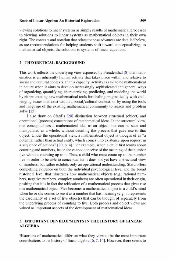
In 1683, Japanese mathematician Seki Kowa developed a version of deter-minants as part of a method for solving a nonlinear system of equations [16].This method was described in a way that relied on the positions of coefficientsarranged in a rectangular array, an indicator of the strong influence of Chinesemathematics on Japanese mathematics. Mikami [16] recreated Seki’s illustra-tion from the original manuscript for 2 x 2 and 3 x 3 cases as shown below inFigure 1 with the following explanation:

Figure 1. Mikami’s recreation of Seki’s diagrams.

1Methods for solving more than one equation through substitution and eliminationwere developed during the 1500s through the works of Cardano, Stifel, Buteo, Gosselin,and others. (See [12] for a treatment of this.)

Roots of Linear Algebra: An Historical Exploration 511

The dotted and real lines, or the red and black lines in the original manuscript, areused to indicate the signs which the product of the elements connected by theselines, will take in the development, the dotted lines corresponding to the positivesign and the real lines to the negative sign, if all the elements be positive. (p. 12)

A 2 x 2 example illustrates how this process yields a determinant as onewould expect to see it today, although with a reversal of sign. Thus

becomes –ad+bc because a and d are connected by a ‘‘real’’ (solid) line, sotheir product takes a negative sign whereas b and c are connected by a dottedline, so their product takes on a positive sign.

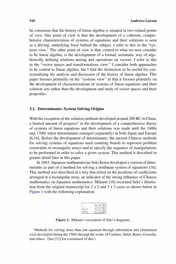
In 1750, Swiss mathematician Gabriel Cramer independently developed away of specifying the solution to a system of linear equations as a set of closed-form expressions comprised purely of fixed but unspecified coefficients of thegiven system. (See [13] for a treatment of this.) Determinants can be seen inthe denominators of these expressions, and Cramer generalized a method fortheir computation by leveraging the combinatorics of cleverly superscripted butunspecified coefficients. The representation Cramer [5] used to denote a systemof equations with as many equations as unknowns is shown below in Figure 2.The upper case Zis, Yis, Xis, Vis denote coefficients while the lower case z,y, x, v denote unknowns. Note that Cramer’s use of superscripts is consistentwith contemporary use of subscripts in that they denote indexing (rather thanexponentiation).

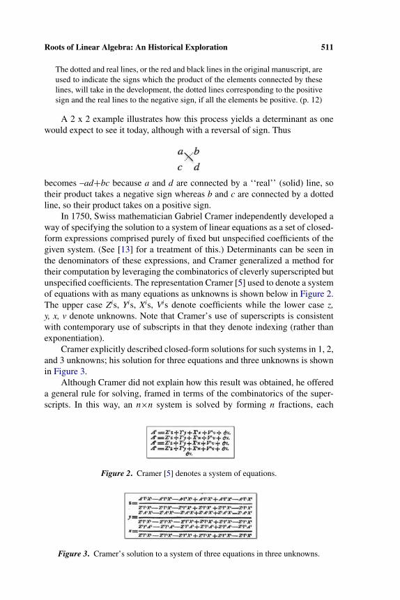
Cramer explicitly described closed-form solutions for such systems in 1, 2,and 3 unknowns; his solution for three equations and three unknowns is shownin Figure 3.

Although Cramer did not explain how this result was obtained, he offereda general rule for solving, framed in terms of the combinatorics of the super-scripts. In this way, an n×n system is solved by forming n fractions, each

Figure 2. Cramer [5] denotes a system of equations.

Figure 3. Cramer’s solution to a system of three equations in three unknowns.

512 Andrews-Larson

of which has n! terms in both the numerator and denominator. Katz [13]includes a translation of Cramer’s description of how the denominators (i.e.,determinants) are computed:

Each term is composed of the coefficient letters, for example ZYX, always writ-ten in the same order, but the indexes are permuted in all possible ways. The signis determined by the rule that if in any given permutation the number of times alarger number precedes a smaller number is even, then the sign is “+” otherwiseit is “-”. [13, p. 192]

Cramer noted that a zero denominator indicates that the system does nothave a unique solution [13]. Furthermore, he specified that in the case that thedenominator and all of the numerators are zero, the system will have infinitelymany solutions, whereas when the denominator is zero but any one of thenumerators is nonzero, the system will have no solution.

I argue that Cramer’s approach would have been impossible without a shiftin the use of algebraic notation introduced by French mathematician FrançoisViète in the late-16th century. The use of literal symbols (e.g., using a variablesuch as x to represent an unknown fixed quantity, a fixed but unspecified quan-tity, or a varying quantity) was revolutionized in 1591 when Viete introducedthe convention of using vowels to represent unknown quantities and conso-nants to represent quantities that are known but unspecified [3]. The particularsof his convention are no longer in use, but the distinction that arose was pivotalin shaping contemporary algebraic notation. This advance can be thought of asthe specification of the idea of a parameter [3].

For both Seki and Cramer, the way in which their notational system struc-tured the coefficients shaped the way the determinant was specified. Seki’sarticulation of the determinant leveraged the physical arrangement of the coef-ficients in order to specify the operations to be performed on those coefficients.Cramer’s articulation of the determinant relied on the clever use of index-ing in the coefficients to create a closed-form expression. It is plausible thatCramer’s notational system affords an object view of systems of equationsmore strongly than does Seki’s, per Cramer’s observation about what the valueof the determinant reveals about the solution to the system.

3.2. Euler’s Inclusive Dependence

A second important development in the theory of systems of linear equa-tions also took place in 1750. Swiss mathematician Leonhard Euler questionedwhether a system of n linear equations with n unknowns has a unique solution,using the following system of equations as a counterexample: 3x − 2y = 5and 4y = 6x − 10 [6]. This observation was made as part of a discussion ofCramer’s paradox, which deals with the number of points of intersection ofalgebraic curves and the number of points needed to determine an algebraic

Roots of Linear Algebra: An Historical Exploration 513

curve. Euler gave additional examples with larger systems, and pointed out thatit is possible for an equation to be “comprised of” or “contained in” others [6,p. 7]. Dorier tags this notion of Euler’s with the term “inclusive dependence,”pointing out that our modern notion of linear dependence is more carefullydefined and more sophisticated [6, p. 7]. The very language that an equationmight be “contained in” or “comprised of” others suggests that early concep-tions of linear dependence involved thinking of dependence as a property of anequation, or perhaps as a relationship between or among equations – rather thanthinking of it as a property of a set of equations. Readers who have taught lin-ear algebra will likely recall hearing students make analogous comments aboutcertain vectors that are “dependent on” other vectors (rather than stating thatthose certain vectors are linear combinations of the other vectors, as the math-ematician in us might hope). I posit that this is a natural, intuitive, informalway of conceptualizing notions of dependence, and that it is a useful concep-tion that can serve as a basis for formalization. Historically speaking, Euler’sobservation certainly raised an issue that contributed to the development of ourcurrent conception of linear dependence.

Both Cramer’s and Euler’s work around systems of linear equations tookplace in the context of theory of curves, and although their observations differin focus, both point to a central related issue. Cramer’s comment identi-fies what the value of his denominators (i.e., the determinant) reveals aboutthe uniqueness of the solution set to a square system of equations, whereasEuler’s inclusive dependence points to the lack of a unique solution when thereis redundancy of information in the equations themselves (perhaps implic-itly assuming the same number of equations as unknowns). The relationshipbetween Cramer’s comment about determinants and Euler’s observation aboutinclusive dependence is an important idea in any introductory linear algebraclass; namely, that a consistent square system will have “inclusive dependence”(as Euler would describe it) if and only if it has infinitely many solutions (whichis when Cramer’s denominators or the determinant is zero).

Like Cramer’s observation, Euler’s observation is significant in that itmarks a qualitative shift in perspective from his predecessors’ process viewof solutions – his reasoning identified properties of the system itself that heldimplications for the system’s solution set. Euler’s observation contrasts withearlier perspectives where mathematical reasoning focused primarily on thedevelopment and use of processes for solving linear systems, and shifts towarda notion of a solution to a system of equations as a mathematical object withits own properties (in this case, uniqueness).

3.3. Other Important Developments

In 1811, Gauss developed a method of least squares for finding the bestapproximate solution to an over-determined (and inconsistent) system of linear

514 Andrews-Larson

equations that had 12 equations and six unknowns. This system of equationsused observational measurements to model the orbit of a celestial body. It wasin this context that Gauss outlined the method of Gaussian elimination, whichhe developed without the use of matrices [10]. His discussion in this and ear-lier works reflects a complete understanding of the conditions under which asystem has no solution, a unique solution, and infinitely many solutions. Forinstance, Gauss gave a detailed explanation of the relationship between elim-ination and the nature of the solution set to a system of linear equations inhis 1809 Theoria Motus (Theory on the Motion of Heavenly Bodies moving inConic Sections):

We have, therefore, as many linear equations as there are unknown quantitiesto be determined, from which the values of the latter will be obtained by com-mon elimination. Let us see now, whether this elimination is always possible, orwhether the solution can become indeterminate, or even impossible. It is known,from the theory of elimination, that the second or third case will occur when oneof the equations . . . being omitted, an equation can be formed from the rest,either identical with the omitted one or inconsistent with it, or, which amounts tothe same thing, when it is possible to assign a linear function αP+βQ+γ R+δS+etc., which is identically either equal to zero, or, at least, free from all theunknown quantities. [9, p. 269].

Thus, we see that Gauss did understand that any system of linear equations canhave no solution, a unique solution, or infinitely many solutions. Furthermore,he explained how one can identify the nature of the solution set based onthe elimination process. He did not give a detailed explanation of Gaussianelimination in this 1809 work, but one appeared in an 1811 piece. Gaussianelimination, in the form in which it was originally proposed in 1811, is dis-cussed in greater detail later in this paper. Recall that Gauss did not use matricesfor notating systems of equations or performing elimination.

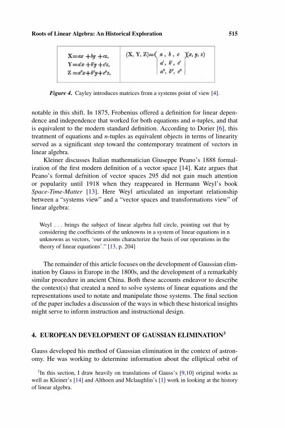
Unlike in Chinese and Japanese traditions, matrices did not come into usein Western mathematics until the late 1800s. The term matrix was coined in1850 by the English mathematician James Joseph Sylvester, who was doingwork with determinants.2 In 1857, Sylvester’s friend and colleague ArthurCayley published his Treatise on the Theory of Matrices [4]. In this treatise,Cayley introduced matrices from a systems of equations point of view (asshown in Figure 4), and then proceeded to develop his theory of matrices asmathematical objects that could be added, multiplied, inverted, and so on.

It was not until the late 1800s that we see a shift from a systems view of lin-ear algebra to a vector spaces view, and the work of Frobenius and Peano were

2Determinants were studied extensively in Western Europe prior to this, e.g., thedescription earlier in this paper regarding Cramer’s work 100 years earlier. A morecomplete discussion of the history of determinants in Western Europe is beyond thescope of this paper but is summarized by Katz [13].

Roots of Linear Algebra: An Historical Exploration 515

Figure 4. Cayley introduces matrices from a systems point of view [4].

notable in this shift. In 1875, Frobenius offered a definition for linear depen-dence and independence that worked for both equations and n-tuples, and thatis equivalent to the modern standard definition. According to Dorier [6], thistreatment of equations and n-tuples as equivalent objects in terms of linearityserved as a significant step toward the contemporary treatment of vectors inlinear algebra.

Kleiner discusses Italian mathematician Giuseppe Peano’s 1888 formal-ization of the first modern definition of a vector space [14]. Katz argues thatPeano’s formal defnition of vector spaces 295 did not gain much attentionor popularity until 1918 when they reappeared in Hermann Weyl’s bookSpace-Time-Matter [13]. Here Weyl articulated an important relationshipbetween a “systems view” and a “vector spaces and transformations view” oflinear algebra:

Weyl . . . brings the subject of linear algebra full circle, pointing out that byconsidering the coefficients of the unknowns in a system of linear equations in nunknowns as vectors, ‘our axioms characterize the basis of our operations in thetheory of linear equations’.” [13, p. 204]

The remainder of this article focuses on the development of Gaussian elim-ination by Gauss in Europe in the 1800s, and the development of a remarkablysimilar procedure in ancient China. Both these accounts endeavor to describethe context(s) that created a need to solve systems of linear equations and therepresentations used to notate and manipulate those systems. The final sectionof the paper includes a discussion of the ways in which these historical insightsmight serve to inform instruction and instructional design.

4. EUROPEAN DEVELOPMENT OF GAUSSIAN ELIMINATION3

Gauss developed his method of Gaussian elimination in the context of astron-omy. He was working to determine information about the elliptical orbit of

3In this section, I draw heavily on translations of Gauss’s [9,10] original works aswell as Kleiner’s [14] and Althoen and Mclaughlin’s [1] work in looking at the historyof linear algebra.

516 Andrews-Larson

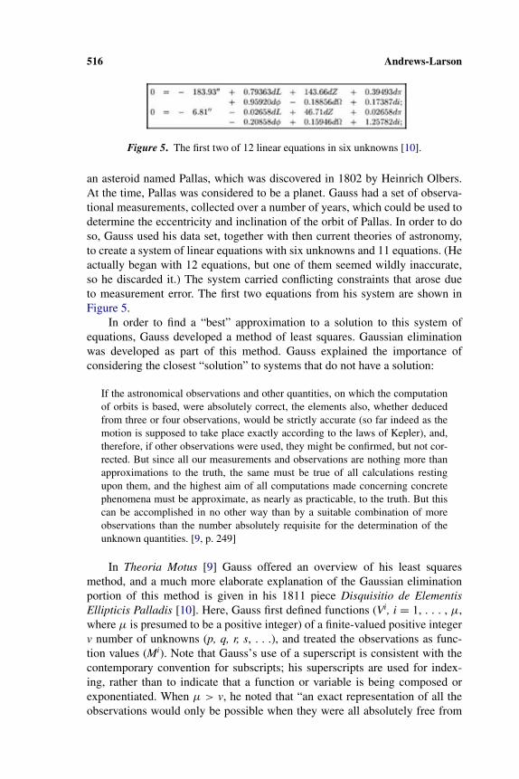
Figure 5. The first two of 12 linear equations in six unknowns [10].

an asteroid named Pallas, which was discovered in 1802 by Heinrich Olbers.At the time, Pallas was considered to be a planet. Gauss had a set of observa-tional measurements, collected over a number of years, which could be used todetermine the eccentricity and inclination of the orbit of Pallas. In order to doso, Gauss used his data set, together with then current theories of astronomy,to create a system of linear equations with six unknowns and 11 equations. (Heactually began with 12 equations, but one of them seemed wildly inaccurate,so he discarded it.) The system carried conflicting constraints that arose dueto measurement error. The first two equations from his system are shown inFigure 5.

In order to find a “best” approximation to a solution to this system ofequations, Gauss developed a method of least squares. Gaussian eliminationwas developed as part of this method. Gauss explained the importance ofconsidering the closest “solution” to systems that do not have a solution:

If the astronomical observations and other quantities, on which the computationof orbits is based, were absolutely correct, the elements also, whether deducedfrom three or four observations, would be strictly accurate (so far indeed as themotion is supposed to take place exactly according to the laws of Kepler), and,therefore, if other observations were used, they might be confirmed, but not cor-rected. But since all our measurements and observations are nothing more thanapproximations to the truth, the same must be true of all calculations restingupon them, and the highest aim of all computations made concerning concretephenomena must be approximate, as nearly as practicable, to the truth. But thiscan be accomplished in no other way than by a suitable combination of moreobservations than the number absolutely requisite for the determination of theunknown quantities. [9, p. 249]

In Theoria Motus [9] Gauss offered an overview of his least squaresmethod, and a much more elaborate explanation of the Gaussian eliminationportion of this method is given in his 1811 piece Disquisitio de ElementisEllipticis Palladis [10]. Here, Gauss first defined functions (Vi, i = 1, . . . , μ,where μ is presumed to be a positive integer) of a finite-valued positive integerv number of unknowns (p, q, r, s, . . .), and treated the observations as func-tion values (Mi). Note that Gauss’s use of a superscript is consistent with thecontemporary convention for subscripts; his superscripts are used for index-ing, rather than to indicate that a function or variable is being composed orexponentiated. When μ > v, he noted that “an exact representation of all theobservations would only be possible when they were all absolutely free from

Roots of Linear Algebra: An Historical Exploration 517

error . . . this cannot, in the nature of things, happen” [9, p. 254]. Gauss arguedthat the most probable values of the unknowns are those such that the sum ofthe squares of the differences between the computed and observed values of thefunctions (i.e., the sum of the squares of the errors ei defined as ei = Vi−Mi)is minimized. By expressing the functions in general linear form (Vi = ni +aip + biq + cir + dis + . . . for real numbers ni, ai, bi, ci, di . . . with i = 1,. . . , μ) and noting that the sum of squares of the errors is minimized whenthe partial derivatives (with respect to unknowns p, q, r, s, . . .) are all zero,Gauss obtained a system of equations in terms of the errors ei, each of whichcan be expressed in terms of unknowns p, q, r, s, . . . Rewriting this system ofequations in terms of p, q, r, s, Gauss subsequently described how the first vari-able p can be eliminated from the system of equations. He then described howone can continue eliminating one variable at a time until only one remains, atwhich point one could determine the value of the single unknown quantity andperform back substitution to determine the values of the other unknowns.

The central aspect of this process that is relevant to the contemporary treat-ment of Gaussian elimination is the sequential use of substitutions performedin such a way that one variable is removed with each step of the process untilonly one variable in one linear equation remains. The value of this single vari-able can then be determined from the equation, and the value is then substitutedinto the previous equation with two unknowns to solve; this process is repeateduntil all unknown values have been found [1].

5. SOLVING LINEAR SYSTEMS IN ANCIENT CHINA

The Nine Chapters on the Mathematical Art is an ancient Chinese text com-prised of 246 problems and solution methods. It is believed to have beenproduced sometime between 200 BC and 50 AD. An earlier version of the textwas burned during the reign of Emperor Ch’in Shih Huang, a controversiallytyrannical ruler credited with the unification of China as well as constructionof the Great Wall of China [24]. The problems in this text arose from contextssuch as field measurement (which gives rise to the development of geometry,fractions, and square and cube roots); trade, commerce, and taxation (whichgive rise to the development of ratios, proportions, and systems of equations);and distance–rate–time problems.

5.1. China’s Mathematical Toolbox ∼200 BC

In order to contextualize the mathematics that appears in the Nine Chapters,it is important to consider the mathematical tools and ideas that the Chinesehad at their disposal at the time it was written. One of the most prominentmathematical tools in common use around 200 BC in China was the counting

518 Andrews-Larson

board, on which counting rods made of bamboo or ivory were arranged in rect-angular arrays so that various calculations could be performed [21]. Countingrod arithmetic was the central method of calculation in Chinese mathematicsbeginning around 500 BC and continuing until it was gradually replaced by theabacus between 1368 and 1644 AD [21]. Common calculations included addi-tion, subtraction, multiplication, and division. Standard algorithms for thesecalculations leveraged the structure of the base-10 system, much like com-mon algorithms of today, although the procedures looked rather different thantoday’s standard column arithmetic.

In addition to the use of counting boards and a base-10 number system,the Chinese also made use of positive and negative integers, as well as frac-tions. They did not use literal symbols to represent unknown or unspecifiedquantities, nor did they use a system of axiomatic deductive logic.

5.2. Linear Systems in the Nine Chapters

In analyzing the ancient Chinese methods for solving linear equations, Shen,Crossley, and Lun [21] noted that the Chinese had as many as seven differentsolution methods. There is some amount of overlap among these methods, andseveral of them only work in systems with one or two equations. In what fol-lows I focus on only one of these methods: the more general method for solvingsystems of linear equations discussed in the problems in Chapter 8, whose titlecan be translated as “Rectangular Arrays.”

Chapter 8 contains 18 problems, all of which correspond to linear systemswith between two and six unknown quantities. With one exception, all of theproblems have a unique solution with the number of constraints (equations)equaling the number of unknown quantities. The only exception to this was aproblem whose solution set had one degree of freedom, which the author dealtwith by adding a reasonable assumption to the context in the description of thesolution.

5.3. Solving Linear Systems with Rectangular Arrays: An Example

A look at the translation of the Nine Chapters produced by Shen et al.[21] offers some insight into the types of contexts that gave rise to systemsof linear equations in ancient China. Thirteen of the eighteen problems inChapter 8 draw on agricultural contexts, dealing with quantities of livestockor grain (by number, weight, volume, or cost). The others contexts range frompractical (pulling forces of horses, amounts of water used by families sharing acommunal well, and amounts of chicken eaten by people based on their socialclass) to more riddle-like (combinations of different types of coins, weightsof sparrows and swallows). These are evidence of the existence of a commoncurrency for trade, the domestication of horses for use as beasts of burden,

Roots of Linear Algebra: An Historical Exploration 519

and the class structure of Chinese society around 200 BC. The first problem inChapter 8 reads:

Now given 3 bundles of top grade paddy, 2 bundles of medium grade paddy,[and] 1 bundle of low grade paddy. Yield: 39 dou of grain. 2 bundles of top gradepaddy, 3 bundles of medium grade paddy, [and] 1 bundle of low grade paddy,yield 34 dou. 1 bundle of top grade paddy, 2 bundles of medium grade paddy,[and] 3 bundles of low grade paddy, yield 26 dou. Tell: how much paddy doesone bundle of each grade yield. [21, p. 399]

In order to fully understand the context of this problem, it is important that thereader understand that paddy is grain and that dou is a unit used for measuringvolume. If we were to rephrase the first sentence in a more contemporary way,it might read “A combination of 3 bundles of high-quality grain, 2 bundles ofmedium-quality grain, and 1 bundle of low-quality grain will yield 39 barrelsof flour.”

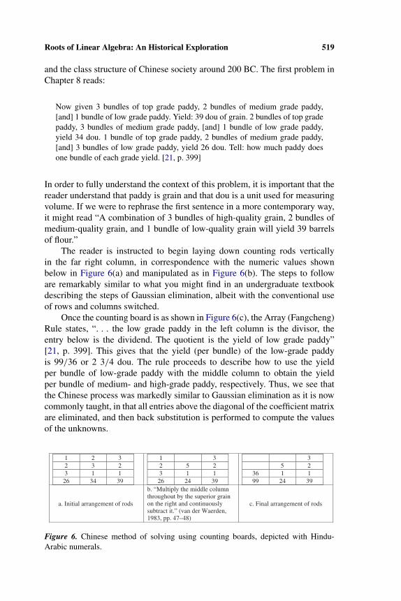
The reader is instructed to begin laying down counting rods verticallyin the far right column, in correspondence with the numeric values shownbelow in Figure 6(a) and manipulated as in Figure 6(b). The steps to followare remarkably similar to what you might find in an undergraduate textbookdescribing the steps of Gaussian elimination, albeit with the conventional useof rows and columns switched.

Once the counting board is as shown in Figure 6(c), the Array (Fangcheng)Rule states, “. . . the low grade paddy in the left column is the divisor, theentry below is the dividend. The quotient is the yield of low grade paddy”[21, p. 399]. This gives that the yield (per bundle) of the low-grade paddyis 99/36 or 2 3/4 dou. The rule proceeds to describe how to use the yieldper bundle of low-grade paddy with the middle column to obtain the yieldper bundle of medium- and high-grade paddy, respectively. Thus, we see thatthe Chinese process was markedly similar to Gaussian elimination as it is nowcommonly taught, in that all entries above the diagonal of the coefficient matrixare eliminated, and then back substitution is performed to compute the valuesof the unknowns.

1 2 32 3 23 1 1

26 34 39

1 32 5 23 1 1

26 24 39

35 2

36 1 199 24 39

a. Initial arrangement of rods

b. “Multiply the middle columnthroughout by the superior grainon the right and continuouslysubtract it.” (van der Waerden,1983, pp. 47–48)

c. Final arrangement of rods

Figure 6. Chinese method of solving using counting boards, depicted with Hindu-Arabic numerals.

520 Andrews-Larson

5.4. Discussion

In the Chinese method, the quantities do not function as coefficients in a sys-tem of equations as we would conceive of them today. For instance, we wouldlikely express the far right column as the equation 3x + 2y + z = 39, wherex is the yield of one bundle of top-grade paddy, y is the yield of one bun-dle of medium-grade paddy, and z is the yield of one bundle of low-gradepaddy. I argue that coefficients of three, two, and one can be conceptualizedin two ways. Based on the problem statement, they are obviously the givennumbers of bundles of each quality of grain. However, these coefficients canalso be viewed as the weights on the unknown yield rates x, y, and z. This latterconceptualization highlights the multiplicative relation between the number ofbundles and the yield per bundle, as well as the additive relationship betweenthe yields from each type of grain in each given combination. I contend itis likely more conceptually difficult for students (though not unimportant) torepresent this situation with a system of equations than it would be for themto represent it with a counting board, as the counting board may mask theneed to explicitly contend with and coordinate these additive and multiplicativerelationships.

In using rectangular arrays to solve linear systems of equations, the centraldemand on the mathematical thinker is that he or she determines a solution tothe system of equations. Mathematical activity is thus focused on the processof finding a solution. I argue that, in Sfard’s [20] framing, this is an example ofa context that promotes a process view of a solution to a system of linear equa-tions. Furthermore, it seems that the way in which systems were representedafforded this intuitive, elimination-based problem-solving approach while alsoconstraining the opportunity to view these linear systems or their solutions asmathematical objects in their own right.

6. PEDAGOGICAL RECOMMENDATIONS

History has the potential to inform instruction in a variety of ways. In particular,it can offer insights into difficulties students are likely to encounter, and it canserve as a source of inspiration for the development of tasks that create a needfor the types of mathematical ideas we want students to learn. With these ideasin mind, in this section I discuss implications for instruction that emerged frommy analysis. I begin with some comments relating to the issue of determinantsdiscussed early in this paper. The remainder of my discussion is organizedaround the contexts that gave rise to a need for ideas relating to linear systemsof equations, the ways in which available tools and representations shaped thedevelopment of those ideas, and the identification of central, underlying ideasand questions that drove the development of a coherent theory of systems oflinear equations.

Roots of Linear Algebra: An Historical Exploration 521

6.1. Instructional Implication: Reinventing Determinants

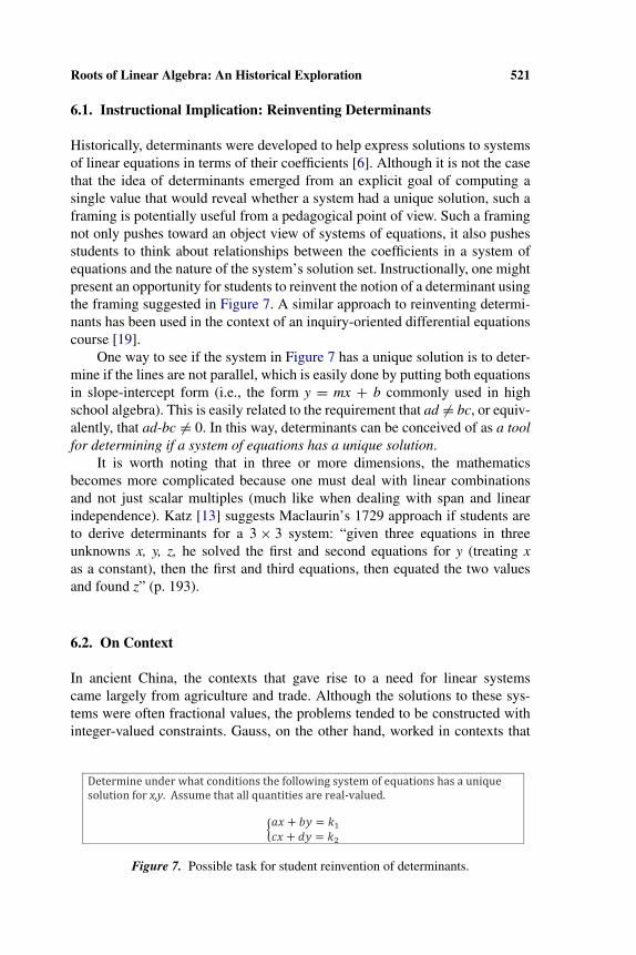
Historically, determinants were developed to help express solutions to systemsof linear equations in terms of their coefficients [6]. Although it is not the casethat the idea of determinants emerged from an explicit goal of computing asingle value that would reveal whether a system had a unique solution, such aframing is potentially useful from a pedagogical point of view. Such a framingnot only pushes toward an object view of systems of equations, it also pushesstudents to think about relationships between the coefficients in a system ofequations and the nature of the system’s solution set. Instructionally, one mightpresent an opportunity for students to reinvent the notion of a determinant usingthe framing suggested in Figure 7. A similar approach to reinventing determi-nants has been used in the context of an inquiry-oriented differential equationscourse [19].

One way to see if the system in Figure 7 has a unique solution is to deter-mine if the lines are not parallel, which is easily done by putting both equationsin slope-intercept form (i.e., the form y = mx + b commonly used in highschool algebra). This is easily related to the requirement that ad �= bc, or equiv-alently, that ad-bc �= 0. In this way, determinants can be conceived of as a toolfor determining if a system of equations has a unique solution.

It is worth noting that in three or more dimensions, the mathematicsbecomes more complicated because one must deal with linear combinationsand not just scalar multiples (much like when dealing with span and linearindependence). Katz [13] suggests Maclaurin’s 1729 approach if students areto derive determinants for a 3 × 3 system: “given three equations in threeunknowns x, y, z, he solved the first and second equations for y (treating xas a constant), then the first and third equations, then equated the two valuesand found z” (p. 193).

6.2. On Context

In ancient China, the contexts that gave rise to a need for linear systemscame largely from agriculture and trade. Although the solutions to these sys-tems were often fractional values, the problems tended to be constructed withinteger-valued constraints. Gauss, on the other hand, worked in contexts that

Figure 7. Possible task for student reinvention of determinants.

522 Andrews-Larson

required non-integer-valued coefficients, and he explicitly discussed the num-bers of possible solutions to linear systems and the conditions under whicheach would occur. He also discussed in detail the need for increased accuracyprovided by using multiple measurements that acknowledge error, and the wayin which this created a system with conflicting constraints for which a “best”solution was needed.

Gauss’s work points to the importance of seriously considering meaning-ful contexts in which the number of constraints (equations) exceeds the numberof unknowns – and the importance of not simply dismissing such systems ashaving no solution. In the case where a system of equations with no solu-tion arises from a meaningful context, there is likely a need to find the bestapproximation to a solution.

In addition to my recommendation, per the work of Gauss, that incon-sistent systems receive their due attention in realistic contexts, I suggest thatinstructors not take it as immediate or obvious that the number of (indepen-dent) constraints needs to equal the number of variables in order to have aunique solution. It is not necessarily obvious to students why the number of(independent) equations must match the number of unknowns in order for a lin-ear system to have a unique solution. For these reasons, I posit that instructorsmight precede the question “How do we solve linear systems of equations?”with “What does it mean to be a solution to a system of equations?” Subsequentclassroom discussions about the following issues could offer insight into howstudents think about processes for solving system of equations.

1. How does the relationship between the number of unknowns and the num-ber of constraints (equations) affect the solution to a system of linearequations?

2. How can we detect and account for conflicting constraints and/or hid-den redundancies when counting the constraints described in the previousquestion?

3. How do we know, when we manipulate systems of equations or performrow/column operations, what information is changed, and what is left thesame? (For instance, if we say two augmented matrices are row equiva-lent, what is equivalent about them, and how do we know that aspect of thesystem was unchanged by the row operations we performed?)

These questions point to a core set of ideas about systems of linear equationsand their solution sets that are non-trivial for students, and are much richerin terms of theory than what a procedurally focused treatment of Gaussianelimination might entail. There is a rich history with a variety of contexts thathave contributed to the development of the current theory of the nature of linearsystems of equations and their solutions – and this set of ideas is a foundationalpart of a complete understanding of linear algebra.

Roots of Linear Algebra: An Historical Exploration 523

6.3. On Tools and Representations

Mathematical tools impact the way in which ideas are notated, represented, andconceptualized. For instance, the use of counting boards in China facilitated ashift to the base-10 numeration system from an earlier system in which thelocation of digits did not indicate their magnitude, and counting boards clearlyaffected the way in which systems of equations were represented and manipu-lated so as to find solutions. Gauss’s use of literal symbols, which distinguishedunknown quantities from unspecified but known quantities, lent itself to theuse of repeated substitutions – a crucial element Gauss’s 1811 description ofhis method for solving linear systems. Differential calculus also served as animportant mathematical tool in Gauss’s development of his method of leastsquares, where his need for Gaussian elimination arose. Another example thatsupports this claim about the importance of mathematical tools is seen in Seki’s‘‘matrix-like’’ arrangement of terms to develop determinants as compared withCramer’s clever use of indexing for his more combinatorial description ofdeterminants.

Pedagogically, this points to the importance of the selection and framing ofmathematical tasks and questions, as well as the notation, representations, andtools used in the posing of those tasks. For instance, consider the Chinese useof rectangular arrays on counting boards to solve what would now be describedas linear systems of equations. The representation is tightly tied to the quan-tities given in the real-world context, and the manipulations of the columnsare easily and intuitively justified in a way that ties directly to the problemcontext. Coherence between problem context and representational tools cansupport students’ problem-solving efforts. On the other hand, representationsthat are too tightly connected to specific contexts and needed manipulationsmay lend themselves more readily to process views as argued previously in thispaper. Process views are developmentally important, but when there is a needto shift to an object view, a shift in notation may help facilitate this change inperspective.

7. FINAL REMARKS

So what is one to do with all this history? How might it inform the teaching oflinear algebra? Some would argue that asking students to work directly with thecontexts from history is a productive route; I would argue that this depends onwhether this approach aligns with the learning goals of a particular course. Theinstructional design theory of Realistic Mathematics Education suggests thatan effective model of supporting students’ learning is by providing them withopportunities to work first in real-world contexts, and to then gradually shiftaway from those specific contexts, pushing students to conjecture what can be

524 Andrews-Larson

generalized and supporting them in shifting toward notation that captures thosegeneralizations [11].

One might then, for instance, draw on the problems such as those given inthe Nine Chapters as contexts for the teaching of row reduction (likely underthe more modern convention in which rows correspond to equations). However,these problems tend to focus on systems with unique solutions. Although thereare some mechanics to learn in row reduction, the insight gleaned from thesystematic use of elimination and how that can extend to situations in which alinear system does not have a unique solution is an important conceptual learn-ing goal, and one that seems to be significantly more troublesome for studentsthan solving a system with a unique solution.

There might also be value in drawing on Gauss’s context to teach abouteither the development of Gaussian elimination or ways of approximating solu-tions to inconsistent systems. However, Gauss’s approach to the former isheavily embedded in a broader set of questions that are beyond the scope of atypical introductory linear algebra course. The latter, the idea of learning aboutways of approximating solutions to inconsistent systems, is a topic with manyrelevant contemporary applications, but is often left as a special topic to be cov-ered as time allows. This is likely due to the fact that, although highly relevantto a number of applied contexts, such approximation methods are not crucialfor developing subsequent ideas in an introductory linear algebra course.

Drawing on my experiences and those of my colleagues interested in issuessurrounding the teaching and learning of linear algebra, a pervasive sourceof student difficulty is describing and making sense of the solution sets tosystems of linear equations which have infinitely many solutions. These dif-ficulties are likely to impede students’ learning of other important ideas inlinear algebra (e.g., describing non-trivial null spaces, finding and interpret-ing eigenvectors). Anecdotally, students are often able to describe a solutionas something that, when “plugged in” for the variables, creates a true state-ment or set of statements; however, when the solution is not a single valuefor each variable, interpretation becomes problematic. Student questions thathave arisen in class discussions around solutions to systems of equations withinfinitely many solutions (after solving systems using substitution and elimina-tion methods, but prior to instruction on row reduction) include: “How do youknow if three planes intersect in a plane or a line?’’and ‘‘ How do you knowhow many parameters there are (for describing the solution set)?’’ and “Howdo you know which variables can be parameters (for describing the solutionset)?” The latter two questions highlight the value of a systematic approach tosolving systems of linear equations that standardizes the choice of parameters(e.g., through row reduction).

Viewed through the lenses of history and mathematics education research,student difficulties with making sense of solution sets that are described usingparameters are perhaps unsurprising. Historically, mathematical understand-ing of linear systems with unique solutions predated our understanding of

Roots of Linear Algebra: An Historical Exploration 525

those with infinitely many solutions. Indeed, notational tools were needed toaccurately and concisely characterize solutions in the latter case. However, theliterature on student thinking would suggest that it is precisely these notationaltools that are one significant source of student struggle. It is well-documentedthat the varied use and interpretation of literal symbols (e.g., as unknowns, asvariables, as parameters) is a source of difficulty for students at the secondaryand tertiary levels [17, 23]. The fact that literal symbols are needed to describesolution sets in the case of systems with infinitely many solutions suggests thatmaking sense of such solution sets would be a source of challenge for students.An example, such as that given by Euler for illustrating inclusive dependence,could prove pedagogically useful for helping students make sense of linear sys-tems with infinitely many solutions as well as the conventions for describingtheir solution sets (both geometrically and algebraically).

Mathematical ideas do not develop until there is an intellectual need forthem, as well as a sufficient set of notational tools to reason effectively in thecontext of that need. A need for a solution to a system of linear equations israther natural, but the idea that some systems do not have unique solutions isperhaps less natural. As such, I argue that in addition to working in contextswith unique solutions, students need opportunities to work with contexts wherean approximate solution to an inconsistent solution is needed, as well as con-texts where they must make sense of parameters. Inconsistent systems couldbe taken from examples, such as that of Gauss, or from any other number ofapplied examples that are commonly used for systems of equations problems inhigh school and college textbooks (e.g., problems where one must relate quanti-ties of particular kinds of food to number of calories from carbohydrates, fats,and proteins). Possani et al. [18] detail how a mathematical modeling prob-lem set in a traffic flow context can be used support students’ learning aboutparameterizations of linear systems with infinitely many solutions.

Looking across the historical development of linear systems, one seesthat the comprehension and articulation of what it means to be a solution toa linear system of equations became more refined and well articulated overtime. Solution sets to linear systems were historically conceptualized first interms of solving processes and subsequently as mathematical objects; students’understanding of solutions is likely to progress similarly. In order to developa conceptual understanding of many of the key ideas in an introductory linearalgebra course, students’ similarly need to come to understand solutions to sys-tems of linear equations as mathematical objects, particularly in the case whenthe solution is not unique. Over 1500 years passed between the articulation ofthe Chinese solution process using counting boards and the general descrip-tions of solution sets that were developed through the theory of determinants(and Euler’s observation about inclusive dependence), so this shift from a pro-cess view of solutions to an object view of solutions is likely to be similarlynon-trivial for students.

526 Andrews-Larson

More research is needed to better understand the nature of difficulties stu-dents experience in coming to understand the solution sets to systems of linearequations, and the rationale for processes that give rise to these solution sets.However, history affords many rich insights into sources of challenge, as wellas ways in which one might recreate the intellectual need for a mathematicalidea in his or her classroom and pair that need with tools that position studentsfor learning based in meaningful, historically informed mathematical activity.

ACKNOWLEDGMENTS

I extend my deepest thanks to Frank Lester, Kathy Clark, and several anony-mous reviewers for help, patience, and guidance in developing this work andfor the invaluable feedback provided on multiple iterations of this paper.

REFERENCES

1. Althoen, S.C. and R. McLaughlin. 1987. Gauss–Jordan reduction: A briefhistory. The American Mathematical Monthly. 94(2): 130–142.

2. Avital, S. 1995. History of mathematics can help improve instruction andlearning. In F. Swetz, J. Fauvel, O. Bekken, B. Johansson, and V. Katz(Eds), Learn from the Masters, pp. 3–12. Washington, DC: MathematicalAssociation of America.

3. Boyer, C. 1985. A History of Mathematics. Princeton, NJ: PrincetonUniversity Press.

4. Cayley, A. 1857. A memoir on the theory of matrices. PhilosophicalTransactions of the Royal Society of London. 148: 17–37.

5. Cramer, G. 1750. Introduction a L’analyse des Lignes CourbesAlgébriques. Geneva: Chez les frères Cramer & Cl. Philibert. Retrieved13 May 2011, from Google Books database.

6. Dorier, J.-L. 2000. Epistemological analysis of the genesis of the theoryof vector spaces. In J.-L. Dorier (Ed.), On the Teaching of Linear Algebra,pp. 3–81. Dordrecht, The Netherlands: Kluwer Academic Publishers.

7. Fearnley-Sander, D. 1979. Hermann Grassmann and the creation of linearalgebra. The American Mathematical Monthly. 86(10): 809–817.

8. Freudenthal, H. 1991. Revisiting Mathematics Education: China Lectures.Dordrecht, The Netherlands: Kluwer Academic Publishers.

9. Gauss, K. 1857. Theory of the Motion of the Heavenly Bodies MovingAbout the Sun in Conic Sections (C.H. Davis, Trans.). Boston, MA: Little,Brown and Company. (Original work published 1809.)

10. Gauss, K. 1957. Work (1803–1826) on the Theory of Least Squares (H.F.Trotter, Trans.). Technical Report No.5, Statistical Techniques Research

Roots of Linear Algebra: An Historical Exploration 527

Group, Princeton, NJ: Princeton University. (Original work published1811.)

11. Gravemeijer, K. 1999. How emergent models may foster the constitu-tion of formal mathematics. Mathematical Thinking and Learning. 1(2):155–177.

12. Heeffer, A. 2010. From the second unknown to the symbolic equation. InA. Heeffer and M. Van Dyck (Eds), Philosophical Aspects of SymbolicReasoning in Early Modern Mathematics, pp. 57–103. London: CollegePublications.

13. Katz, V. J. 1995. Historical ideas in teaching linear algebra. In F. Swetz,J. Fauvel, O. Bekken, B. Johansson, and V. Katz (Eds), Learn from theMasters, pp. 189–206. Washington, DC: Mathematical Association ofAmerica.

14. Kleiner, I. 2007. A History of Abstract Algebra. Boston, MA: Birkhauser.15. Lesh, R. & Doerr, H. 2003. Foundations of a models and modeling

perspective on mathematics teaching, learning, and problem solving. InR. Lesh and H. Doerr (Eds), Beyond Constructivism: Models and ModelingPerspectives on Mathematics Problem Solving, Learning, and Teaching,pp. 3–33. Mahwah, NJ: Lawrence Erlbaum Associates.

16. Mikami, Y. 1914. On the Japanese theory of determinants. Isis. 2(1): 9–36.17. Philipp, R. A. 1992. The many uses of algebraic variables. The

Mathematics Teacher. 85(7): 557–561.18. Possani, E., M. Trigueros, J. G. Preciado, and M. D. Lozano.2010. Use

of models in the teaching of linear algebra. Linear Algebra and itsApplications. 432(8): 2125–2140.

19. Rasmussen, C. 2002. Instructional materials for a first course in dif-ferential equations. Unpublished document. Purdue Calumet University,Hammond, IN.

20. Sfard, A. 1991. On the dual nature of mathematical conceptions:Reflections on processes and objects as different sides of the same coin.Educational Studies in Mathematics. 22(1): 1–36.

21. Shen, K., J. N. Crossley, and A. W.-C. Lun. 1999. The Nine Chapters onthe Mathematical Art: Companion and Commentary. New York: OxfordUniversity Press.

22. Swetz, F. J. 1995. Using problems from the history of mathematics inclassroom instruction. In F. Swetz, J. Fauvel, O. Bekken, B. Johansson,and V. Katz (Eds), Learn From the Masters, pp. 25–38. Washington, DC:Mathematical Association of America.

23. Trigueros, M. and S. Jacobs.2008. On developing a rich conception of vari-able. Making the Connection: Research and Teaching in UndergraduateMathematics Education. 73, 3–13.

24. van der Waerden, B. L. 1983. Geometry and Algebra in AncientCivilizations. Berlin, Germany: Springer-Verlag.

528 Andrews-Larson

BIOGRAPHICAL SKETCH

Christine Andrews-Larson is an Assistant Professor of Mathematics Educationin the College of Education at Florida State University. Her research focuses onteacher learning, with a particular emphasis on teacher workgroups and profes-sional networks. Her dissertation focused on student thinking, modeling, andhistory of mathematics with an eye toward instructional design in the contextof undergraduate linear algebra. Her post-doctoral research focused on oppor-tunities for teacher learning through site-based professional development andteachers’ professional networks in the context of working to improve mid-dle school math instruction at scale. She is currently working to coordinatethese two lines of research for the purpose of understanding how to scale upinquiry-oriented instruction with a focus on post-secondary mathematics.