roptim: General Purpose Optimization with C++ · 2.3. The C++ interface: class Roptim The Roptim class is designed to provide a single, uniﬁed interface for performing general purpose

roptim: An R Package for General Purpose

Optimization with C++

Yi Pan

University of Birmingham

Abstract

In R environment, users can solve general-purpose optimization problems easily usingthe optim function in package stats which is provided by default R installation. Althoughthe implementations of five core algorithms in optim(), namely "Nelder-Mead", "BFGS"

(Broyden-Fletcher-Goldfarb-Shanno), "CG" (conjugate gradients), "L-BFGS-B" (limited-memory BFGS with box constraints) and "SANN" (simulated annealing), are convertedto native machine code, the user-provided objective function and gradient are usuallyevaluated using the R interpreter which may result in performance penalty. This paperdescribes a user-friendly C++ class Roptim from roptim package which provides a unifiedwrapper interface to the C codes of the five optimization algorithms underlying optim

function and enables users performing general purpose optimization tasks using C++

without reimplementing the optimization routines. More advanced features for optimiza-tion tasks, such as checking gradient/Hessian of the objective function and specifying fixedparameters while allowing the rest to be adjusted to minimize the objective function, willalso be discussed in this paper.

Keywords: Nelder-Mead, BFGS, CG, L-BFGS-B, SANN, C++, R.

1. Introduction

Optimization algorithms are frequently used in mathematics, statistics, computer science andoperations research. Most statistical tools (R, Stata, SAS), as well as mathematical softwaresuch as Mathematica, Maple and MATLAB, provide optimization and nonlinear modellingpackages. The R environment (R Core Team 2017) has included build-in optimization al-gorithms since its early days where stats::optim(), or optim() in package stats, is oneof most widely used functions for conducting basic optimization tasks. Here by basic op-timization, we mean minimization of functions that are mostly smooth without any con-straints, or at most bounds-constrained. Within the same package, stats::nlm() (Schnabel,Koonatz, and Weiss 1985) is used for solving nonlinear unconstrained minimization prob-lems and stats::nlminb() offers unconstrained and constrained optimization using PORTroutines (Fox 1997). Outside the stats package, the package optimx (Nash, Varadhan et al.2011) and its successor package optimr (Nash, Varadhan, Grothendieck, Nash, and Yes 2016)offers a replacement and extension of the optim function to unify and streamline optimizationcapabilities in R. Note this paper is not an exhaustive survey of all recent R developments foroptimization, and more complete discussion of functions and packages that perform optimiza-tion tasks can be found in the task view on Optimization and Mathematical Programming

2 roptim: General Purpose Optimization with C++

(Theussl and Borchers 2014).

While the R language provides a stable statistical environment for fast prototyping andeasy data visualization, code implemented in R is interpreted at its core which may re-sult in a much longer execution time when compared to the equivalent program in nativemachine code. Although the five core implementations of algorithms in optim(), namely"Nelder-Mead", "BFGS" (Broyden-Fletcher-Goldfarb-Shanno), "CG" (conjugate gradients),"L-BFGS-B" (limited-memory BFGS with box constraints) and "SANN" (simulated anneal-ing), are converted to high performance machine code, the user-provided objective functionand gradient are usually implemented in R which requires intensive evaluations during theoptimization process. With the increase of function complexity and data size, the executiontime can be a potential issue. To overcome this problem, most experienced R package de-velopers, who use C++ for the core computation, may have to use the C interface for thefive aforementioned methods directly (much harder to use when compared to optim), or evenwrite their own implementation of algorithms to do the optimization tasks.

In this paper, we will focus on the basic function minimization problems using the five afore-mentioned algorithms, and present a user-friendly C++ class Roptim in R package roptim

(freely available from CRAN at http://CRAN.R-project.org/package=roptim) as a wrap-per for the C codes underlying optim to perform optimization tasks. The new approach makeit straight-forward for R users, who are familiar with optim function, to convert their exist-ing code or write new code of optimization tasks in C++ by using the Rcpp (Eddelbuettel,François, Allaire, Chambers, Bates, and Ushey 2011) extension package in conjunction withthe RcppArmadillo C++ matrix library (Eddelbuettel and Sanderson 2014) for numericallinear algebra. The main objective of this paper is to serve as the document of our package(since package roptim is not a conventional package with pure R function interface and itonly provides wrapper classes defined in C++ header files) and introduce the Roptim classto wide audiences of statisticians and practitioners who needs to perform optimization in R

using C++ for faster speed while still want to get consistent results with the optim function.

The rest of this paper is organized as follows. In Section 2 we briefly introduce the basicoptimization problems and five algorithms used in optim, then present both the internal C

interface provided by R and the new proposed C++ interface provided by package roptim.Section 3 provides three optimization problems as examples to illustrate the use of packageand discusses some advanced techniques used in performing the optimization tasks beforeSection 4 concludes the paper with some further discussions.

2. Design of package roptim

2.1. Overview of optimization task

In the simplest case, an optimization problem is about finding the minimization of generalnonlinear smooth functions of n parameters where the values of parameters may subject toconstraints. The task can be formulated as

x∗ = arg minx

f(x) subject to L ≤ x ≤ U (1)

where x ∈ Rn and f : Rn 7→ R. Note that optimization problem with non-smooth objective

function is ongoing research which is beyond the scope of this paper. To solve the problem in

Yi Pan 3

Table 1: Optimization algorithms included in optimAlgorithm C interface Method type Box constraints

Nelder-Mead nmmin Derivative-free NoBFGS vmmin Quasi-Newton No

CG cgmin Gradient NoL-BFGS-B lbfgsb Quasi-Newton Yes

SANN samin Simulated-annealing No

Equation (1), we will focus on the five algorithms and their corresponding implementationswhich are internally used in optim function of stats package (Table 1).

The "Nelder-Mead" method (Nelder and Mead 1965) is from the second edition of Nash(1990) which uses only function values (i.e., derivative-free) and is robust but relatively slow.It works reasonably well for non-differentiable functions.

The "BFGS" (Fletcher 1970) and "L-BFGS-B" (Byrd, Lu, Nocedal, and Zhu 1995) are quasi-Newton methods (also called variable metric algorithms) which require both function valuesand gradients to perform the optimization task. In "BFGS", the inverse Hessian is approx-imated by the Broyden-Fletcher-Goldfarb-Shanno formula at each iteration using updatesspecified by gradient evaluations (or approximate gradient evaluation) and a ’backtrack toacceptable point’ line search is used to the resulting newton step for a new trial solution;while in "L-BFGS-B", the approximation of inverse Hessian is stored implicitly by keeping afew vectors as needed and box optimization is allowed for bounds constraints on parameters.

The "CG" is a conjugate gradients method (Fletcher and Reeves 1964) which also requiresboth function value and gradient for minimization task and three strategies are included fromNash (1990). When compared to BFGS, conjugate gradient methods will generally be morefragile, but as they do not store a matrix they may be successful in much larger optimizationproblems. More detailed discussion for "BFGS", "L-BFGS-B" and "CG" can be found in Wrightand Nocedal (1999).

The "SANN" is by default a variant of simulated annealing (Bélisle 1992) which belongs to theclass of stochastic global optimization methods. This method uses only function values but isrelatively slow since it does not have a termination test and always evaluates the function forthe specified maximum number of iterations. It will also work for non-differentiable functions.This implementation uses the Metropolis function for the acceptance probability. By defaultthe next candidate point is generated from a Gaussian Markov kernel with scale proportionalto the actual temperature.

2.2. The C interface

To avoid the performance penalty when the optimization tasks (i.e., both objective functionand the corresponding gradient) are implemented in R using optim, one possible solution isto make use of the following C interface of five algorithms directly (Team 1999):

• Nelder-Mead:

void nmmin(int n, double *xin, double *x, double *Fmin, optimfn fn,

int *fail, double abstol, double intol, void *ex,


double alpha, double beta, double gamma, int trace,

int *fncount, int maxit);

• BFGS:

void vmmin(int n, double *x, double *Fmin,

optimfn fn, optimgr gr, int maxit, int trace,

int *mask, double abstol, double reltol, int nREPORT,

void *ex, int *fncount, int *grcount, int *fail);

• Conjugate gradients:

void cgmin(int n, double *xin, double *x, double *Fmin,

optimfn fn, optimgr gr, int *fail, double abstol,

double intol, void *ex, int type, int trace,

int *fncount, int *grcount, int maxit);

• Limited-memory BFGS with bounds:

void lbfgsb(int n, int lmm, double *x, double *lower,

double *upper, int *nbd, double *Fmin, optimfn fn,

optimgr gr, int *fail, void *ex, double factr,

double pgtol, int *fncount, int *grcount,

int maxit, char *msg, int trace, int nREPORT);

• Simulated annealing:

void samin(int n, double *x, double *Fmin, optimfn fn, int maxit,

int tmax, double temp, int trace, void *ex);

where users need to supply an objective function and the corresponding gradient separatelyin C with the types of

typedef double optimfn(int n, double *par, void *ex);

typedef void optimgr(int n, double *par, double *gr, void *ex);

respectively when needed. Many of the arguments are common to the various aforementionedmethods — n is the number of parameters, x or xin is the starting parameters on entrywhile x is also the final parameters on exit, with final value returned in Fmin. Most of theother parameters can be found from the help page for optim. However the interface for theC language proves hard to use and debug for even advanced users which makes it much lesspopular when compared to optim function.

We also need to note that, at the time of writing, the provided implementation of "SANN"

actually requires evaluation of an user provided R function internally through argument ex forgenerating a new candidate point which makes it almost impossible to use in C language. Tosolve this issue, we manually changes the original codes for "SANN" to remove the requirementfor R function evaluation and provided it using same interface within our package roptim.

2.3. The C++ interface: class Roptim

The Roptim class is designed to provide a single, unified interface for performing generalpurpose optimization in a similar fashion to optim() so that users of optim function can

Yi Pan 5

easily convert their existing code or implement their optimization tasks in C++ by employingRcpp package and RcppArmadillo package which provide a bidirectional interface between R

and C++ at the object level.

The implementation is provided as a template class within the roptim namespace and canbe defined as

Roptim<YourTask> opt(method);

where implementation of YourTask will be discussed shortly in next section and method shouldbe chosen from "Nelder-Mead", "BFGS", "CG", "L-BFGS-B" and "SANN". For an instance ofRoptim class named as opt, its member functions and variables are listed below.

• opt.set_method(method)

specifies the method to be used. Again, method should be chosen from "Nelder-Mead","BFGS", "CG", "L-BFGS-B" and "SANN".

• opt.set_lower(vec)/opt.set_upper(vec)

sets bounds on the variables for the "L-BFGS-B" method where vec is a arma::vec.

• opt.set_hessian(flag)

Logical. Should a numerically differentiated Hessian matrix be computed?

• opt.minimize(task, par)

performs the optimization task. Here task is an instance of YourTask and par is thevector of starting values with type arma::vec. Once the optimization is finished, par

will be overwritten by the optimized points.

• opt.control.var

control is a public data member of type RoptimControl. Here RoptimControl is aninternal member class (or nested class) of Roptim and defines all control parameterswith public access. Control parameter var can be one of the following variable:

– trace

Non-negative integer. If positive, tracing information on the progress of the opti-mization is produced. Higher values may produce more tracing information: formethod "L-BFGS-B" there are six levels of tracing. (To understand exactly whatthese do see the source code: higher levels give more detail.)

– fnscale

An overall scaling to be applied to the value of objective function and gradientduring optimization. If negative, turns the problem into a maximization problem.Optimization is performed on task(par)/fnscale.

– parscale

A vector of scaling values for the parameters. Optimization is performed onpar/parscale and these should be comparable in the sense that a unit changein any element produces about a unit change in the scaled value.

– ndeps

A vector of step sizes for the finite-difference approximation to the gradient, onpar/parscale scale. Defaults to 1e-3.


– maxit

The maximum number of iterations. Defaults to 100 for the derivative-basedmethods, and 500 for "Nelder-Mead".

For "SANN", maxit gives the total number of function evaluations: there is no otherstopping criterion. Defaults to 10000.

– abstol

The absolute convergence tolerance. Only useful for non-negative functions, as atolerance for reaching zero.

– reltol

Relative convergence tolerance. The algorithm stops if it is unable to reduce thevalue by a factor of reltol * (abs(val) + reltol) at a step. Defaults to 1e-8.

– alpha, beta, gamma

Scaling parameters for the "Nelder-Mead" method. alpha is the reflection factor(default 1.0), beta the contraction factor (0.5) and gamma the expansion factor(2.0).

– REPORT

The frequency of reports for the "BFGS", "L-BFGS-B" and "SANN" methods ifopt.control.trace is positive. Defaults to every 10 iterations for "BFGS" and"L-BFGS-B", or every 100 temperatures for "SANN".

– warn_1d_NelderMead

a logical indicating if the (default) "Nelder-Mead" method should signal a warn-ing when used for one-dimensional minimization. As the warning is sometimesinappropriate, you can suppress it by setting this option to false.

– type

for the conjugate-gradients method. Takes value 1 for the Fletcher-Reeves update,2 for Polak-Ribiere and 3 for Beale-Sorenson.

– lmm

is an integer giving the number of BFGS updates retained in the "L-BFGS-B"

method, It defaults to 5.

– factr

controls the convergence of the "L-BFGS-B" method. Convergence occurs when thereduction in the objective is within this factor of the machine tolerance. Defaultis 1e7, that is a tolerance of about 1e-8.

– pgtol

helps control the convergence of the "L-BFGS-B" method. It is a tolerance on theprojected gradient in the current search direction. This defaults to zero, when thecheck is suppressed.

– temp

controls the "SANN" method. It is the starting temperature for the cooling schedule.Defaults to 10.

– tmax

is the number of function evaluations at each temperature for the "SANN" method.Defaults to 10.

Yi Pan 7

Once the optimization task is done by using opt.minimize(), some remaining member func-tions of Roptim class, for printing or extracting the results, can be used safely.

• opt.print()

prints all relevant results of the optimization task.

• opt.par()

returns the best set of parameters found and has the same values with par which isupdated after we called opt.minimize(task, par).

• opt.value()

returns the corresponding value of function being optimized (i.e., task(par)).

• opt.fncount()

returns the number of objective function evaluation times.

• opt.grcount()

returns the number of gradient evalution times.

• opt.convergence()

An integer code. 0 indicates successful completion (which is always the case for "SANN").Possible error codes are

– 1

indicates that the iteration limit maxit had been reached.

– 10

indicates degeneracy of the Nelder-Mead simplex.

– 51

indicates a warning from the "L-BFGS-B" method; see message for further details.

– 52

indicates an error from the "L-BFGS-B" method; see message for further details.

• opt.message()

returns a character string giving any additional information returned by the optimizer,or NULL.

• opt.hessian()

returns a numerically differentiated hessian matrix.

2.4. The C++ interface: class Functor

In contrast to optim, both objective function and gradient should be stored within a singleclass when using class Roptim. This design may bring additional benefit since it is commonfor the objective function and gradient to have some shared computational part, and wewill discuss it in Section 3.3. The pseudo code below shows how to define a class for youroptimization task with Functor.


struct YourTask : public Functor {

public:

double operator()(const vec &par) override; // objective function

void Gradient(const vec &par, vec &grad) override; // gradient

void Hessian(const vec &par, mat &hess) override; // hessian

};

double YourTask::operator()(const vec &par){

// code for evaluating objective function

}

void YourTask::Gradient(const vec &par, vec &grad){

// code for evaluating gradient

}

void YourTask::Hessian(const vec &par, mat &hess){

// code for evaluating hessian

}

YourTask should be defined as a class derived from an abstract template base class namedFunctor within namespace roptim. It is helpful to know the fact that when our own versionof Gradient() and Hessian() are not defined in class YourTask, we will automatically havethe inherited version of Gradient() and Hessian() from class Functor instead which pro-vide forward-difference approximation of gradient (through task.ApproximateGradient(par,

grad)) and Hessian (through task.ApproximateHessian(par, grad)) respectively. In otherwords, numerical gradient will be generated if a non-derivative-free algorithm is employed.The only exception is that when we use "SANN", the member function Gradient() (whichspecifies the function to generate a new candidate point) will never be used in the optimizationprocess unless we explicit tell it to; See an example in Section 3.2.

Obviously, we need to implement the objective function as it is always needed for optimizationtasks and the call operator is defined as a pure virtual member function in its base classFunctor. We also need to note that the implementation of member function Gradient() isusually required and is only optional for "Nelder-Mead" (it is a derivative-free method) and"SANN" (a default Gaussian Markov kernel is used for generating a new candidate point whenGradient() is not defined) while Hessian() is always optional since none of five algorithmsrequire the evaluation of Hessian matrix during optimization process.

3. Examples

3.1. Rosenbrock function

In this section, we will take Rosenbrock function, which is a non-convex function and used asan example in help page of optim function, to illustrate the use of Roptim class.

The Rosenbrock function is defined by

f(x1, x2) = (1 − x1)2 + 100(x2 − x21)2 (2)

Yi Pan 9

and obviously it has a global minimum of 0 at the point (1, 1). The corresponding class forthis function can be defined as follows.

class Rosen : public Functor {

public:

double operator()(const arma::vec &x) override {

double x1 = x(0);

double x2 = x(1);

return 100 * std::pow((x2 - x1 * x1), 2) + std::pow(1 - x1, 2);

}

void Gradient(const arma::vec &x, arma::vec &gr) override {

gr = arma::zeros<arma::vec>(2);

double x1 = x(0);

double x2 = x(1);

gr(0) = -400 * x1 * (x2 - x1 * x1) - 2 * (1 - x1);

gr(1) = 200 * (x2 - x1 * x1);

}

void Hessian(const arma::vec &x, arma::mat &he) override {

he = arma::zeros<arma::mat>(2, 2);

double x1 = x(0);

double x2 = x(1);

he(0, 0) = -400 * x2 + 1200 * x1 * x1 + 2;

he(0, 1) = -400 * x1;

he(1, 0) = he(0, 1);

he(1, 1) = 200;

}

};

Given the starting values (-1.2, 1), the following C++ function example1_rosen_bfgs() isused to apply the BFGS algorithm for the minimization of Rosenbrock function.

// [[Rcpp::export]]

void example1_rosen_bfgs()

{

Rosen rb;

Roptim<Rosen> opt("BFGS");

opt.control.trace = 1;

opt.set_hessian(true);

arma::vec x = {-1.2, 1};

opt.minimize(rb, x);

Rcpp::Rcout << "-------------------------" << std::endl;


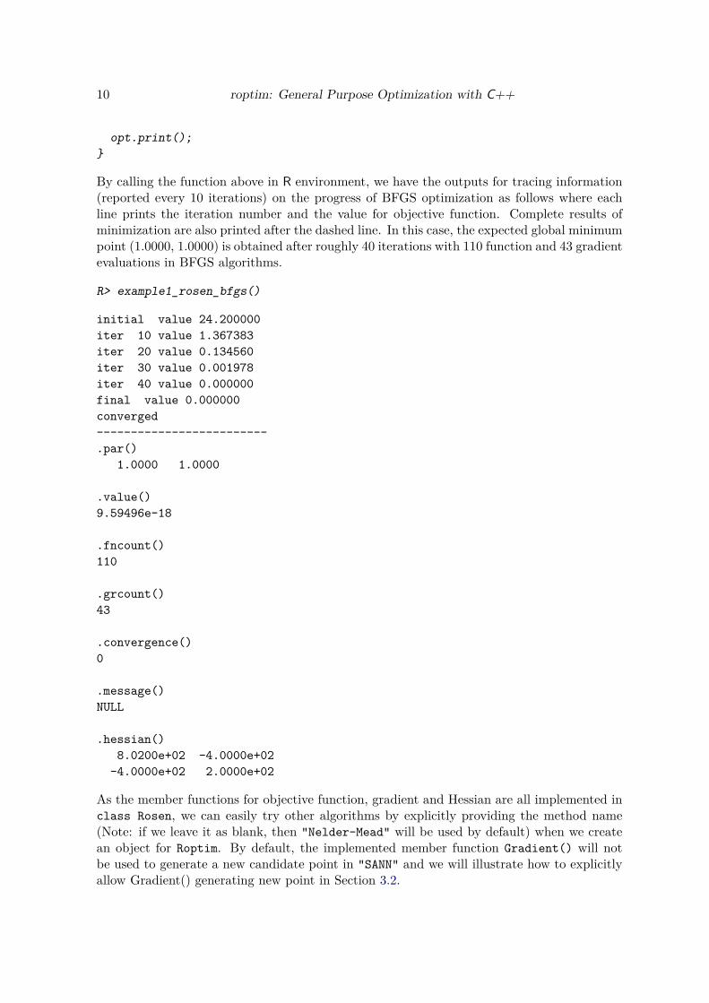
opt.print();

}

By calling the function above in R environment, we have the outputs for tracing information(reported every 10 iterations) on the progress of BFGS optimization as follows where eachline prints the iteration number and the value for objective function. Complete results ofminimization are also printed after the dashed line. In this case, the expected global minimumpoint (1.0000, 1.0000) is obtained after roughly 40 iterations with 110 function and 43 gradientevaluations in BFGS algorithms.

R> example1_rosen_bfgs()

initial value 24.200000

iter 10 value 1.367383




final value 0.000000

converged

-------------------------

.par()

1.0000 1.0000

.value()

9.59496e-18

.fncount()

110

.grcount()

43

.convergence()

0

.message()

NULL

.hessian()

8.0200e+02 -4.0000e+02

-4.0000e+02 2.0000e+02

As the member functions for objective function, gradient and Hessian are all implemented inclass Rosen, we can easily try other algorithms by explicitly providing the method name(Note: if we leave it as blank, then "Nelder-Mead" will be used by default) when we createan object for Roptim. By default, the implemented member function Gradient() will notbe used to generate a new candidate point in "SANN" and we will illustrate how to explicitlyallow Gradient() generating new point in Section 3.2.

Yi Pan 11

// [[Rcpp::export]]

void example1_rosen_other_methods()

{

Rosen rb;

arma::vec x;

// "Nelder-Mead": converged

Roptim<Rosen> opt1;

x = {-1.2, 1};

opt1.minimize(rb, x);

opt1.print();

// "CG": did not converge in the default number of steps

Roptim<Rosen> opt2("CG");

x = {-1.2, 1};


opt2.print();

// "CG": did not converge in the default number of steps

Roptim<Rosen> opt3("CG");

opt3.control.type = 2;

x = {-1.2, 1};


opt3.print();

// "L-BFGS-B"

Roptim<Rosen> opt4("L-BFGS-B");

x = {-1.2, 1};


opt4.print();

// "SANN"

Roptim<Rosen> opt5("SANN");

x = {-1.2, 1};


opt5.print();

}

The gradient and Hessian computation proves to be notoriously difficult to debug and get themright with the increased complexity of functions. Sometimes a subtly buggy implementationwill manage to learn something that can look surprisingly reasonable while performing less wellthan the correct one. It is possible (but not recommended) to define a class RosenNoGrad

without the implementation for gradient and still apply the non-gradient-free algorithms (e.g.BFGS).

class RosenNoGrad : public Functor {

public:



double x1 = x(0);

double x2 = x(1);

return 100 * std::pow((x2 - x1 * x1), 2) + std::pow(1 - x1, 2);

}

};

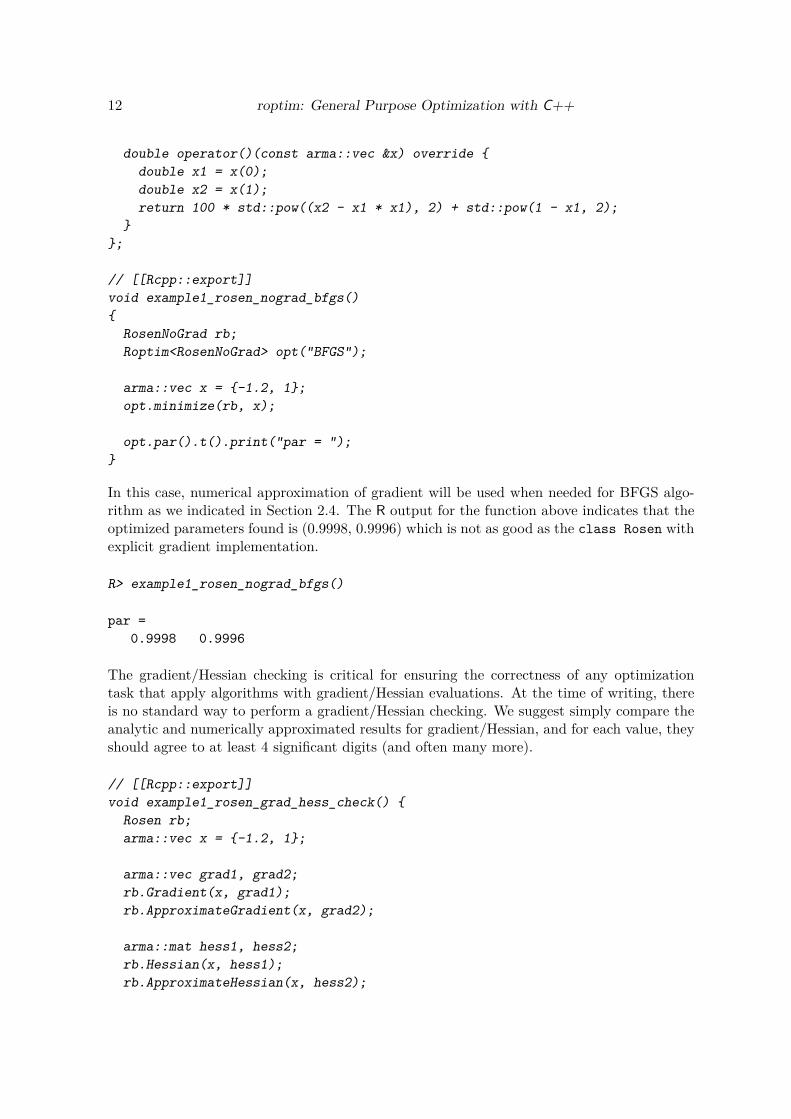
// [[Rcpp::export]]

void example1_rosen_nograd_bfgs()

{

RosenNoGrad rb;

Roptim<RosenNoGrad> opt("BFGS");

arma::vec x = {-1.2, 1};

opt.minimize(rb, x);

opt.par().t().print("par = ");

}

In this case, numerical approximation of gradient will be used when needed for BFGS algo-rithm as we indicated in Section 2.4. The R output for the function above indicates that theoptimized parameters found is (0.9998, 0.9996) which is not as good as the class Rosen withexplicit gradient implementation.

R> example1_rosen_nograd_bfgs()

par =

0.9998 0.9996

The gradient/Hessian checking is critical for ensuring the correctness of any optimizationtask that apply algorithms with gradient/Hessian evaluations. At the time of writing, thereis no standard way to perform a gradient/Hessian checking. We suggest simply compare theanalytic and numerically approximated results for gradient/Hessian, and for each value, theyshould agree to at least 4 significant digits (and often many more).

// [[Rcpp::export]]

void example1_rosen_grad_hess_check() {

Rosen rb;

arma::vec x = {-1.2, 1};

arma::vec grad1, grad2;

rb.Gradient(x, grad1);

rb.ApproximateGradient(x, grad2);

arma::mat hess1, hess2;

rb.Hessian(x, hess1);

rb.ApproximateHessian(x, hess2);

Yi Pan 13

Rcpp::Rcout << "Gradient checking" << std::endl;

grad1.t().print("analytic:");

grad2.t().print("approximate:");


Rcpp::Rcout << "Hessian checking" << std::endl;

hess1.print("analytic:");

hess2.print("approximate:");

}

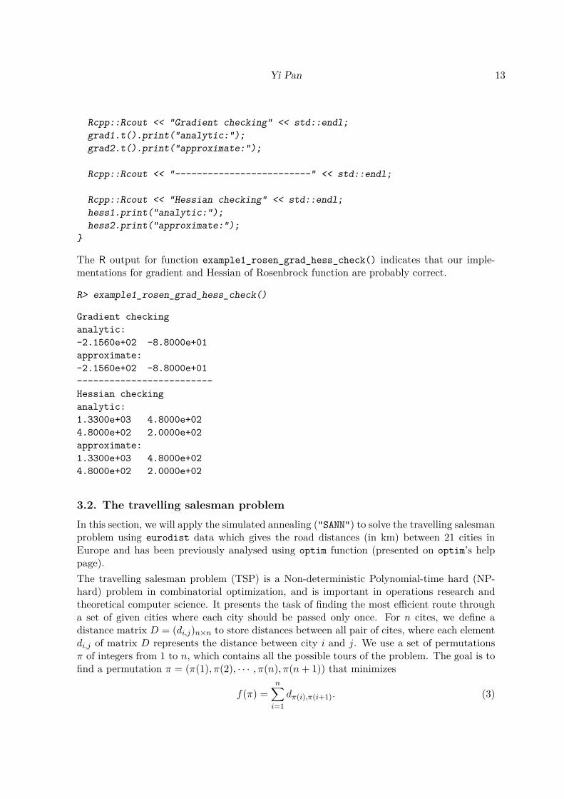
The R output for function example1_rosen_grad_hess_check() indicates that our imple-mentations for gradient and Hessian of Rosenbrock function are probably correct.

R> example1_rosen_grad_hess_check()

Gradient checking

analytic:

-2.1560e+02 -8.8000e+01

approximate:

-2.1560e+02 -8.8000e+01

-------------------------

Hessian checking

analytic:

1.3300e+03 4.8000e+02

4.8000e+02 2.0000e+02

approximate:

1.3300e+03 4.8000e+02

4.8000e+02 2.0000e+02

3.2. The travelling salesman problem

In this section, we will apply the simulated annealing ("SANN") to solve the travelling salesmanproblem using eurodist data which gives the road distances (in km) between 21 cities inEurope and has been previously analysed using optim function (presented on optim’s helppage).

The travelling salesman problem (TSP) is a Non-deterministic Polynomial-time hard (NP-hard) problem in combinatorial optimization, and is important in operations research andtheoretical computer science. It presents the task of finding the most efficient route througha set of given cities where each city should be passed only once. For n cites, we define adistance matrix D = (di,j)n×n to store distances between all pair of cites, where each elementdi,j of matrix D represents the distance between city i and j. We use a set of permutationsπ of integers from 1 to n, which contains all the possible tours of the problem. The goal is tofind a permutation π = (π(1), π(2), · · · , π(n), π(n + 1)) that minimizes

f(π) =n

∑

i=1

dπ(i),π(i+1). (3)


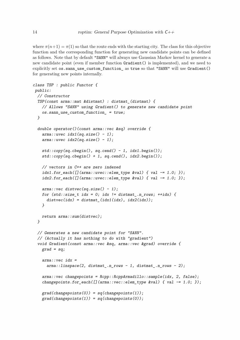
where π(n+1) = π(1) so that the route ends with the starting city. The class for this objectivefunction and the corresponding function for generating new candidate points can be definedas follows. Note that by default "SANN" will always use Gaussian Markov kernel to generate anew candidate point (even if member function Gradient() is implemented), and we need toexplicitly set os.sann_use_custom_function_ as true so that "SANN" will use Gradient()

for generating new points internally.

class TSP : public Functor {

public:

// Constructor

TSP(const arma::mat &distmat) : distmat_(distmat) {

// Allows "SANN" using Gradient() to generate new candidate point

os.sann_use_custom_function_ = true;

}

double operator()(const arma::vec &sq) override {

arma::uvec idx1(sq.size() - 1);

arma::uvec idx2(sq.size() - 1);

std::copy(sq.cbegin(), sq.cend() - 1, idx1.begin());

std::copy(sq.cbegin() + 1, sq.cend(), idx2.begin());

// vectors in C++ are zero indexed

idx1.for_each([](arma::uvec::elem_type &val) { val -= 1.0; });

idx2.for_each([](arma::uvec::elem_type &val) { val -= 1.0; });

arma::vec distvec(sq.size() - 1);

for (std::size_t idx = 0; idx != distmat_.n_rows; ++idx) {

distvec(idx) = distmat_(idx1(idx), idx2(idx));

}

return arma::sum(distvec);

}

// Generates a new candidate point for "SANN".

// (Actually it has nothing to do with "gradient")

void Gradient(const arma::vec &sq, arma::vec &grad) override {

grad = sq;

arma::vec idx =

arma::linspace(2, distmat_.n_rows - 1, distmat_.n_rows - 2);

arma::vec changepoints = Rcpp::RcppArmadillo::sample(idx, 2, false);

changepoints.for_each([](arma::vec::elem_type &val) { val -= 1.0; });

grad(changepoints(0)) = sq(changepoints(1));

grad(changepoints(1)) = sq(changepoints(0));

Yi Pan 15

}

private:

arma::mat distmat_;

};

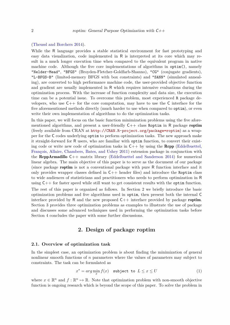
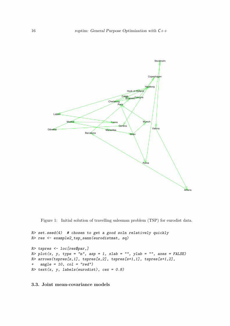
We present in Figure 1 the initial solution of travelling salesman problem where the sequenceis generated according to the alphabetic orders of 21 cities:

R> sq <- c(1:nrow(eurodistmat), 1) # Initial sequence: alphabetic

R> distance(sq)

R> # rotate for conventional orientation

R> loc <- -cmdscale(eurodist, add = TRUE)$points

R> x <- loc[,1]; y <- loc[,2]

R> s <- seq_len(nrow(eurodistmat))

R> tspinit <- loc[sq,]

R>

R> plot(x, y, type = "n", asp = 1, xlab = "", ylab = "", axes = FALSE)

R> arrows(tspinit[s,1], tspinit[s,2], tspinit[s+1,1], tspinit[s+1,2],

+ angle = 10, col = "green")

R> text(x, y, labels(eurodist), cex = 0.8)

and obviouly it is not the best route for TSP.

Given the eurodist data and initial solution (i.e., stating values), the following C++ functionexample2_tsp_sann() is used to apply the simulated annealling algorithm for solving thetravelling salesman problem.

// [[Rcpp::export]]

Rcpp::List example2_tsp_sann(arma::mat eurodistmat, arma::vec x) {

TSP dist(eurodistmat);

Roptim<TSP> opt("SANN");

opt.control.maxit = 30000;

opt.control.temp = 2000;

opt.control.trace = true;

opt.control.REPORT = 500;

opt.minimize(dist, x);


opt.print();

return Rcpp::List::create(Rcpp::Named("par") = x);

}

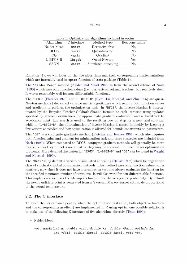
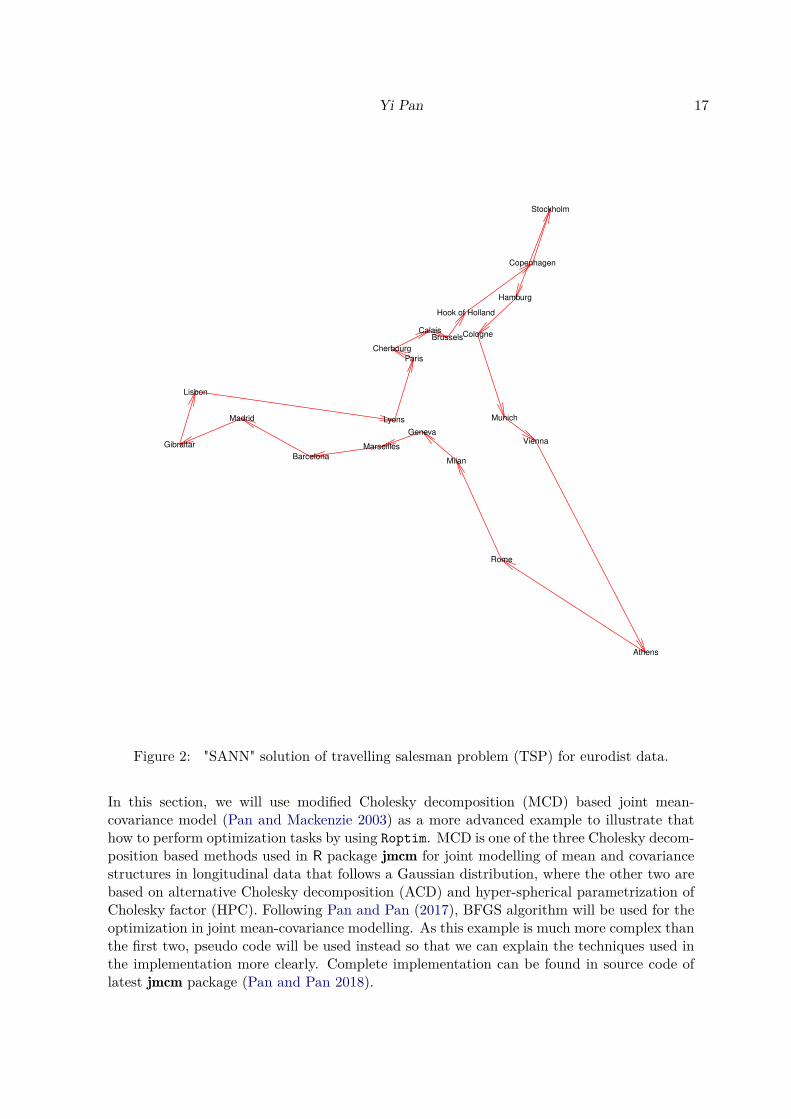
By calling the function above in R environment, we can obtain the optimized parameters toplot the new route which is presented in Figure 2.


Athens

Barcelona

BrusselsCalais

Cherbourg

Cologne

Copenhagen

Geneva

Gibraltar

Hamburg

Hook of Holland

Lisbon

LyonsMadrid

Marseilles

Milan

Munich

Paris

Rome

Stockholm

Vienna

Figure 1: Initial solution of travelling salesman problem (TSP) for eurodist data.

R> set.seed(4) # chosen to get a good soln relatively quickly

R> res <- example2_tsp_sann(eurodistmat, sq)

R> tspres <- loc[res$par,]

R> plot(x, y, type = "n", asp = 1, xlab = "", ylab = "", axes = FALSE)

R> arrows(tspres[s,1], tspres[s,2], tspres[s+1,1], tspres[s+1,2],

+ angle = 10, col = "red")

R> text(x, y, labels(eurodist), cex = 0.8)

3.3. Joint mean-covariance models

Yi Pan 17

Athens

Barcelona

BrusselsCalais

Cherbourg

Cologne

Copenhagen

Geneva

Gibraltar

Hamburg

Hook of Holland

Lisbon

LyonsMadrid

Marseilles

Milan

Munich

Paris

Rome

Stockholm

Vienna

Figure 2: "SANN" solution of travelling salesman problem (TSP) for eurodist data.

In this section, we will use modified Cholesky decomposition (MCD) based joint mean-covariance model (Pan and Mackenzie 2003) as a more advanced example to illustrate thathow to perform optimization tasks by using Roptim. MCD is one of the three Cholesky decom-position based methods used in R package jmcm for joint modelling of mean and covariancestructures in longitudinal data that follows a Gaussian distribution, where the other two arebased on alternative Cholesky decomposition (ACD) and hyper-spherical parametrization ofCholesky factor (HPC). Following Pan and Pan (2017), BFGS algorithm will be used for theoptimization in joint mean-covariance modelling. As this example is much more complex thanthe first two, pseudo code will be used instead so that we can explain the techniques used inthe implementation more clearly. Complete implementation can be found in source code oflatest jmcm package (Pan and Pan 2018).


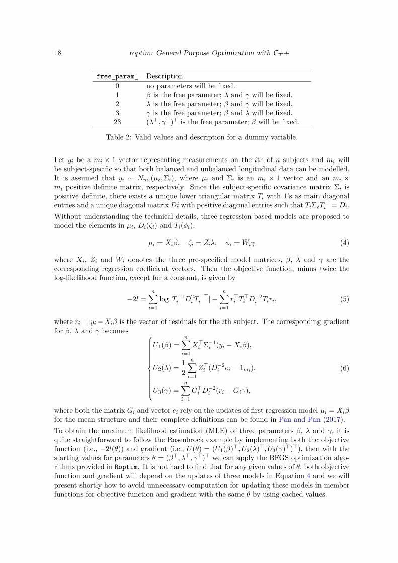
free_param_ Description

0 no parameters will be fixed.1 β is the free parameter; λ and γ will be fixed.2 λ is the free parameter; β and γ will be fixed.3 γ is the free parameter; β and λ will be fixed.23 (λ⊤, γ⊤)⊤ is the free parameter; β will be fixed.

Table 2: Valid values and description for a dummy variable.

Let yi be a mi × 1 vector representing measurements on the ith of n subjects and mi willbe subject-specific so that both balanced and unbalanced longitudinal data can be modelled.It is assumed that yi ∼ Nmi

(µi, Σi), where µi and Σi is an mi × 1 vector and an mi ×mi positive definite matrix, respectively. Since the subject-specific covariance matrix Σi ispositive definite, there exists a unique lower triangular matrix Ti with 1’s as main diagonalentries and a unique diagonal matrix Di with positive diagonal entries such that TiΣiT

⊤i = Di.

Without understanding the technical details, three regression based models are proposed tomodel the elements in µi, Di(ζi) and Ti(φi),

µi = Xiβ, ζi = Ziλ, φi = Wiγ (4)

where Xi, Zi and Wi denotes the three pre-specified model matrices, β, λ and γ are thecorresponding regression coefficient vectors. Then the objective function, minus twice thelog-likelihood function, except for a constant, is given by

−2l =n

∑

i=1

log |T −1i D2

i T −⊤

i | +n

∑

i=1

r⊤

i T ⊤

i D−2i Tiri, (5)

where ri = yi − Xiβ is the vector of residuals for the ith subject. The corresponding gradientfor β, λ and γ becomes

U1(β) =n

∑

i=1

X⊤

i Σ−1i (yi − Xiβ),

U2(λ) =1

2

n∑

i=1

Z⊤

i (D−2i ei − 1mi

),

U3(γ) =n

∑

i=1

G⊤

i D−2i (ri − Giγ),

(6)

where both the matrix Gi and vector ei rely on the updates of first regression model µi = Xiβ

for the mean structure and their complete definitions can be found in Pan and Pan (2017).

To obtain the maximum likelihood estimation (MLE) of three parameters β, λ and γ, it isquite straightforward to follow the Rosenbrock example by implementing both the objectivefunction (i.e., −2l(θ)) and gradient (i.e., U(θ) = (U1(β)⊤, U2(λ)⊤, U3(γ)⊤)⊤), then with thestarting values for parameters θ = (β⊤, λ⊤, γ⊤)⊤ we can apply the BFGS optimization algo-rithms provided in Roptim. It is not hard to find that for any given values of θ, both objectivefunction and gradient will depend on the updates of three models in Equation 4 and we willpresent shortly how to avoid unnecessary computation for updating these models in memberfunctions for objective function and gradient with the same θ by using cached values.

Yi Pan 19

As suggested in Pan and Mackenzie (2003), the actual algorithm is a bit more sophisticatedsince the three parameters are asymptotically independent. In other words, it is possible toupdate the parameter one by one in each iteration with the other two fixed. At the sametime, two parameters β and γ have the following explicit updating forms,

β = (n

∑

i=1

X⊤

i Σ−1i Xi)

−1n

∑

i=1

X⊤

i Σ−1i yi,

γ = (n

∑

i=1

G⊤

i D−2i Gi)

−1n

∑

i=1

G⊤

i D−2i ri,

(7)

and λ is the only parameter that need to be updated by performing the numerical optimiza-tion. Ideally, we require a class MCD that is able to keep the value of β and γ fixed so thatwe can perform the BFGS optimization on λ easily. It is achieved by introducing a dummyvariable named free_param_ whose valid values and corresponding descriptions are listedin Table 2. Note that value 23 for free_param_ is not used in our example since the twoparameters λ and γ are asymptotically independent in MCD, but in ACD/HPC it is not thesame case and these two parameters should be optimized together. A simplified version ofclass MCD is provided as follows.

class MCD : public Functor {

public:


UpdateMCD(x);

// implementation of objective function

}

void Gradient(const arma::vec &x, arma::vec &grad) override {

UpdateMCD(x);

if (free_param_ == 0) {

arma::vec grad1, grad2, grad3;

GradientBeta(grad1);

GradientLambda(grad2);

GradientGamma(grad3);

grad = concatenate(grad1, grad2, grad3);

} else if (free_param_ == 1) {

GradientBeta(grad);


GradientLambda(grad);


GradientGamma(grad);

}

}

GardientBeta(arma::vec &grad1) { // implementation of U1 }

GradientLambda(arma::vec &grad2) { // implementation of U2 }

GradientGamma(arma::vec &grad3) { // implementation of U3 }


void UpdateMCD(const arma::vec &x);

void UpdateBeta() {

// implementation of updating form for beta

set_free_param(1); // 1. fix values of lambda and gamma temporarily

// by setting free_param_ to 1

UpdateMCD(beta); // 2. update parameters and models in the cache

set_free_param(0); // 3. set free_param_ back to default value 0

}

void UpdateGamma() {

// implementation of updating form for gamma

set_free_param(3); // 1. fix values of beta and lambda temporarily


UpdateMCD(gamma); // 2. update parameters and models in the cache

set_free_param(0); // 3. set free_param_ back to default value 0

}

void set_free_param(int val) { free_param_ = val; }

private:

int free_param_ = 0;

arma::mat X_, Z_, W_; // model matrices

arma::vec theta_, beta_, lambda_, gamma_; // cached parameters

arma::mat Xbta_, Zlmd_, Wgma_; // cache for three regression models

};

In contrast to class Rosen, both the member functions of call operator (i.e., objective func-tion) and Gradient() in MCD called UpdateMCD() at the very beginning which is intendedto check whether the supplied parameter x is different from its cached value, if yes, updatethe parameters and three regression models in the cache accordingly. Similarly, the memberfunction UpdateMCD() is also used in UpdateBeta() and UpdateGamma() to keep values ofparameters and models in the cache updated after updating the value of β and γ respectively.The internal behaviour of UpdateMCD() is largely controlled by the value of free_param_ andits full implementation should be as follows.

void MCD::UpdateMCD(const arma::vec &x) {

// Step 1. Compare x with cached value for parameters

// and decide if update is necessary

bool update_flag = true;

if (free_param_ == 0 && IsEqual(x, theta_)) {

update_flag = false;

} else if (free_param_ == 1 && IsEqual(x, beta_)) {


} else if (free_param_ == 2 && IsEqual(x, lambda_)) {


} else if (free_param_ == 3 && IsEqual(x, gamma_)) {


Yi Pan 21

}

// Step 2. Update values in the cache when needed

if (update_flag) {

// Step 2.1. Update cached parameters


theta _ = x;

// also update beta_, lambda_ & gamma_


beta_ = x;

// also update theta_


lambda_ = x;



gamma_ = x;


}

// Step 2.2. Update three regression models in the cache


Xbta_ = X_ * beta_;

Zlmd_ = Z_ * lambda_;

Wgam_ = W_ * gamma_;


Xbta_ = X_ * beta_;


Zlmd_ = Z_ * lambda_;


Wgam_ = W_ * gamma_;

}

}

}

It is not unusual for objective function and gradient having some common computation parts,and defining them within the same class make it possible to avoid unnecessary computation bystoring the results of common part in the cache and update them only when it is necessary.The use of dummy variable free_param_ enables us to change the behaviour of memberfunctions for objective function and gradient so that we can optimize some parameters withothers fixed. To minimize the objective function −2l(θ) and obtain the MLE of θ, we caneasily apply the profile (i.e., estimating parameters one by one with other parameters fixed ineach iteration) and non-profile approaches; See Appendix B for the comparison of these twoapproaches using two real datasets.

void mcdfit (...) {

MCD mcd; // Create an instance of mcd


// by default, free_param_ should be set to 0

Roptim<MCD> opt("BFGS");

arma::vec x = start_value; // the starting values for theta

if (profile) {

// Initializations

for (std::size_t iter = 0; iter != kMaxIteration; ++iter) {

// Update beta and values in the cache

mcd.UpdateBeta();

// Set parameter lambda from x

// Optimize lambda and update values in the cache

mcd.set_free_param(2); // 1. fix values of beta and gamma temporarily


opt.minimize(mcd, lambda); // 2. perform the optimization on lambda

mcd.UpdateMCD(lambda); // 3. update parameters and models in cache

mcd.set_free_param(0); // 4. set free_param_ back to default value 0

// Update gamma and values in the cache

mcd.UpdateGamma();

// Compare x with updated theta in mcd

// If a pre-specified criterion is met, break the for loop

// else update x with theta

}

} else {

opt.minimize(mcd, x);

}

}

The actual implementation for class MCD, ACD, HPC and the utility function for model fittingare more complex as the three Cholesky based methods share quite a lot in common and weeven created a base class named JmcmBase and a model fitting class named JmcmFit for themto avoid code duplication.

4. Conclusion

In this paper, we have illustrated the use of class Roptim and discussed some advancedtechniques used in implementation for optimization tasks. By using this new approach, R

users who are familiar with optim can easily convert their existing code or write new code ofoptimization tasks in C++ for much faster speed and still get consistent results.

References

Yi Pan 23

Bélisle CJ (1992). “Convergence theorems for a class of simulated annealing algorithms onRd.” Journal of Applied Probability, 29(4), 885–895.

Byrd RH, Lu P, Nocedal J, Zhu C (1995). “A limited memory algorithm for bound constrainedoptimization.” SIAM Journal on Scientific Computing, 16(5), 1190–1208.

Eddelbuettel D, François R, Allaire J, Chambers J, Bates D, Ushey K (2011). “Rcpp: SeamlessR and C++ integration.” Journal of Statistical Software, 40(8), 1–18.

Eddelbuettel D, Sanderson C (2014). “RcppArmadillo: Accelerating R with high-performanceC++ linear algebra.” Computational Statistics & Data Analysis, 71, 1054–1063.

Fletcher R (1970). “A new approach to variable metric algorithms.” The computer journal,13(3), 317–322.

Fletcher R, Reeves CM (1964). “Function minimization by conjugate gradients.” The computerjournal, 7(2), 149–154.

Fox P (1997). “The Port Mathematical Subroutine Library, Version 3.” URL http://www.bell-labs. com/project/PORT.

Nash JC (1990). Compact numerical methods for computers: linear algebra and functionminimisation. CRC press.

Nash JC, Varadhan R, Grothendieck G, Nash MJC, Yes L (2016). “Package ’optimr’.”

Nash JC, Varadhan R, et al. (2011). “Unifying optimization algorithms to aid software systemusers: optimx for R.” Journal of Statistical Software, 43(9), 1–14.

Nelder JA, Mead R (1965). “A simplex method for function minimization.” The computerjournal, 7(4), 308–313.

Pan J, Mackenzie G (2003). “On modelling mean-covariance structures in longitudinal stud-ies.” Biometrika, 90(1), 239–244.

Pan J, Pan Y (2017). “jmcm: An R Package for Joint Mean-Covariance Modeling of Longi-tudinal Data.” Journal of Statistical Software, 82(9), 1–29.

Pan J, Pan Y (2018). jmcm: Joint Mean-Covariance Models using Armadillo and S4. R

package version 0.1.8.0, URL https://CRAN.R-project.org/package=jmcm.

R Core Team (2017). R: A Language and Environment for Statistical Computing. R Founda-tion for Statistical Computing, Vienna, Austria. URL https://www.R-project.org/.

Schnabel RB, Koonatz JE, Weiss BE (1985). “A modular system of algorithms for uncon-strained minimization.” ACM Transactions on Mathematical Software (TOMS), 11(4),419–440.

Team RC (1999). “Writing R extensions.” R Foundation for Statistical Computing.

Theussl S, Borchers H (2014). “CRAN task view: Optimization and mathematical program-ming.” Technical report, Version 2014-08-08, URL http://CRAN. R-project. org/view=Optimization.

Wright SJ, Nocedal J (1999). “Numerical optimization.” Springer Science, 35(67-68), 7.


A. Reimplementing two simple optimization tasks in C++

There are in total four examples given on the document page of optim() to demonstrateits useage of performing general optimization tasks. We have discussed the first and secondexample (i.e., minimizing Rosenbrock function and solving txravelling salesman problem)using our new approach in Section 3.1 and 3.2 respectively. The remaining two problemswill be illustrated here as simple examples of reimplementing R code of minimization tasksin C++.

The third example provided by roptim() is given as follows:

R> flb <- function(x)

R> { p <- length(x); sum(c(1, rep(4, p-1)) * (x - c(1, x[-p])^2)^2) }

R> ## 25-dimensional box constrained

R> optim(rep(3, 25), flb, NULL, method = "L-BFGS-B",

R> lower = rep(2, 25), upper = rep(4, 25)) # par[24] is *not* at boundary

and same results can be obtained by calling the following C++ function in R environment:

class Flb : public Functor {

public:


int p = x.size();

arma::vec part1 = arma::ones<arma::vec>(p) * 4;

part1(0) = 1;

arma::vec tmp = arma::ones<arma::vec>(p);

std::copy(x.cbegin(), x.cend() - 1, tmp.begin() + 1);

arma::vec part2 = arma::pow(x - arma::pow(tmp, 2), 2);

return arma::dot(part1, part2);

}

};

// [[Rcpp::export]]

void example3_flb_25_dims_box_con() {

Flb f;

arma::vec lower = arma::ones<arma::vec>(25) * 2;

arma::vec upper = arma::ones<arma::vec>(25) * 4;

Roptim<Flb> opt("L-BFGS-B");

opt.set_lower(lower);

opt.set_upper(upper);

opt.control.trace = 1;

arma::vec x = arma::ones<arma::vec>(25) * 3;

Yi Pan 25

opt.minimize(f, x);


opt.print();

}

The fourth example provided by roptim() is given as follows:

R> ## "wild" function , global minimum at about -15.81515

R> fw <- function (x)

R> 10*sin(0.3*x)*sin(1.3*x^2) + 0.00001*x^4 + 0.2*x+80

R> res <- optim(50, fw, method = "SANN",

R> control = list(maxit = 20000, temp = 20, parscale = 20))

R> res

R> ## Now improve locally {typically only by a small bit}:

R> (r2 <- optim(res$par, fw, method = "BFGS"))

and similar results (as "SANN" is used) can be obtained by calling the following C++ functionin R environment:

class Fw : public Functor {

public:

double operator()(const arma::vec &xval) override {

double x = arma::as_scalar(xval);

return 10 * std::sin(0.3 * x) * std::sin(1.3 * std::pow(x, 2.0)) +

0.00001 * std::pow(x, 4.0) + 0.2 * x + 80;

}

};

// [[Rcpp::export]]

void example4_wild_fun() {

Fw f;

Roptim<Fw> opt("SANN");

opt.control.maxit = 20000;

opt.control.temp = 20;

opt.control.parscale = 20;

arma::vec x = {50};

opt.minimize(f, x);

x.print();

Roptim<Fw> opt2("BFGS");

opt2.minimize(f, x);

x.print();

}


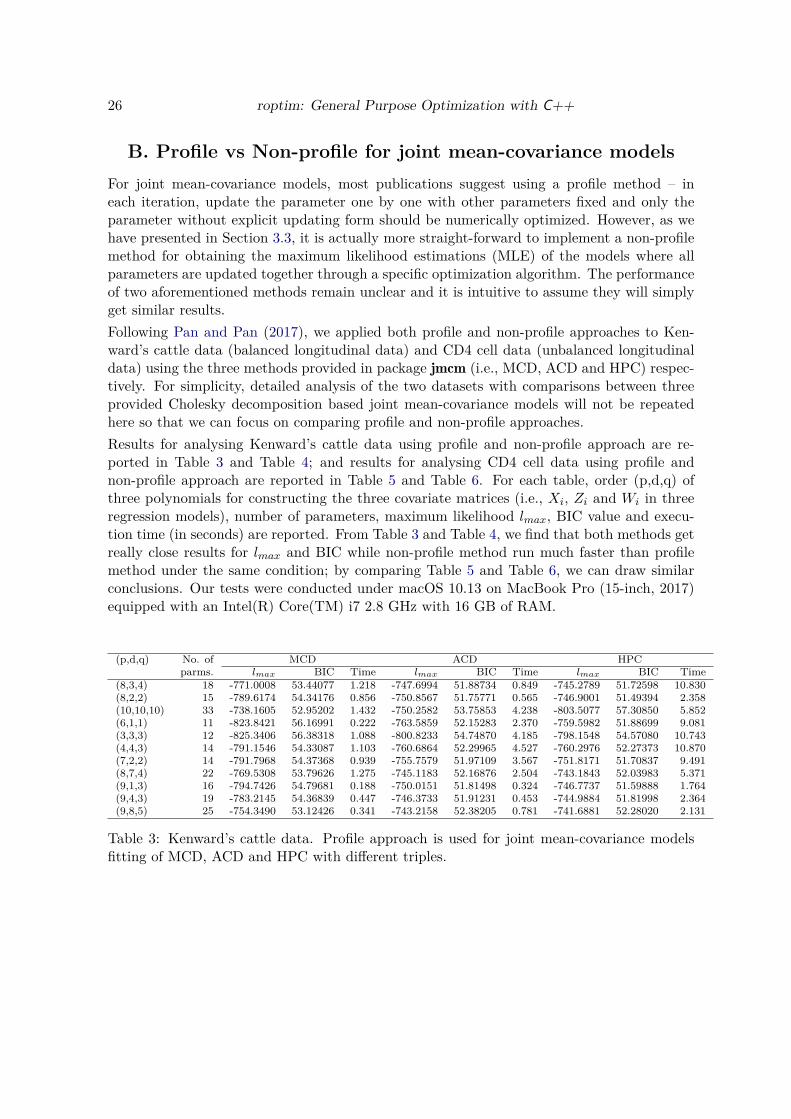
B. Profile vs Non-profile for joint mean-covariance models

For joint mean-covariance models, most publications suggest using a profile method – ineach iteration, update the parameter one by one with other parameters fixed and only theparameter without explicit updating form should be numerically optimized. However, as wehave presented in Section 3.3, it is actually more straight-forward to implement a non-profilemethod for obtaining the maximum likelihood estimations (MLE) of the models where allparameters are updated together through a specific optimization algorithm. The performanceof two aforementioned methods remain unclear and it is intuitive to assume they will simplyget similar results.

Following Pan and Pan (2017), we applied both profile and non-profile approaches to Ken-ward’s cattle data (balanced longitudinal data) and CD4 cell data (unbalanced longitudinaldata) using the three methods provided in package jmcm (i.e., MCD, ACD and HPC) respec-tively. For simplicity, detailed analysis of the two datasets with comparisons between threeprovided Cholesky decomposition based joint mean-covariance models will not be repeatedhere so that we can focus on comparing profile and non-profile approaches.

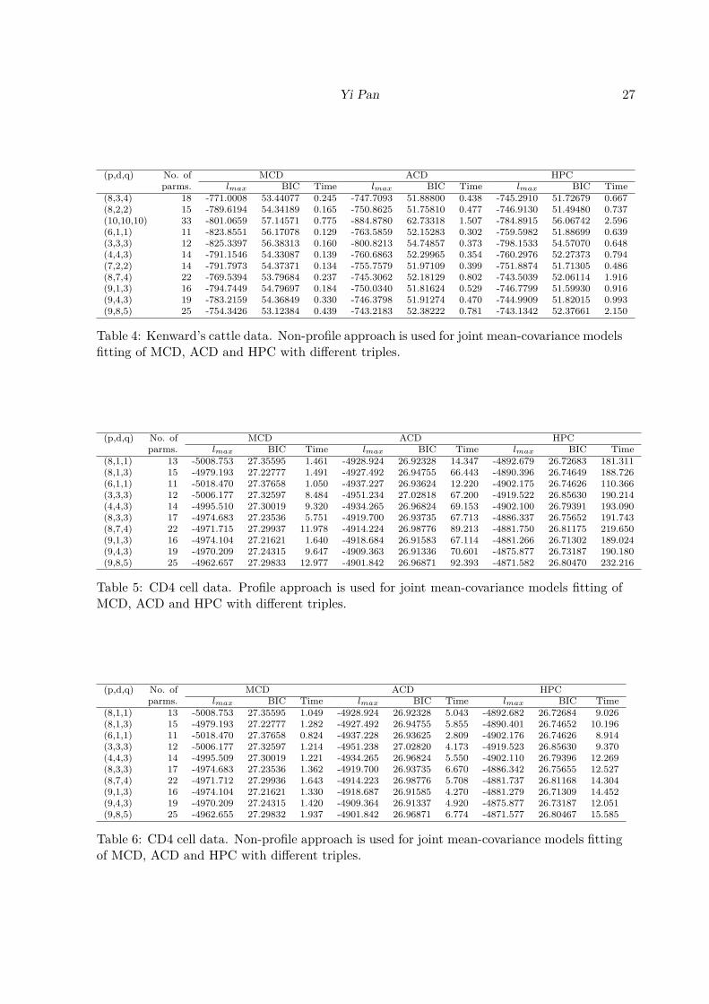
Results for analysing Kenward’s cattle data using profile and non-profile approach are re-ported in Table 3 and Table 4; and results for analysing CD4 cell data using profile andnon-profile approach are reported in Table 5 and Table 6. For each table, order (p,d,q) ofthree polynomials for constructing the three covariate matrices (i.e., Xi, Zi and Wi in threeregression models), number of parameters, maximum likelihood lmax, BIC value and execu-tion time (in seconds) are reported. From Table 3 and Table 4, we find that both methods getreally close results for lmax and BIC while non-profile method run much faster than profilemethod under the same condition; by comparing Table 5 and Table 6, we can draw similarconclusions. Our tests were conducted under macOS 10.13 on MacBook Pro (15-inch, 2017)equipped with an Intel(R) Core(TM) i7 2.8 GHz with 16 GB of RAM.

(p,d,q) No. of MCD ACD HPCparms. lmax BIC Time lmax BIC Time lmax BIC Time

(8,3,4) 18 -771.0008 53.44077 1.218 -747.6994 51.88734 0.849 -745.2789 51.72598 10.830(8,2,2) 15 -789.6174 54.34176 0.856 -750.8567 51.75771 0.565 -746.9001 51.49394 2.358(10,10,10) 33 -738.1605 52.95202 1.432 -750.2582 53.75853 4.238 -803.5077 57.30850 5.852(6,1,1) 11 -823.8421 56.16991 0.222 -763.5859 52.15283 2.370 -759.5982 51.88699 9.081(3,3,3) 12 -825.3406 56.38318 1.088 -800.8233 54.74870 4.185 -798.1548 54.57080 10.743(4,4,3) 14 -791.1546 54.33087 1.103 -760.6864 52.29965 4.527 -760.2976 52.27373 10.870(7,2,2) 14 -791.7968 54.37368 0.939 -755.7579 51.97109 3.567 -751.8171 51.70837 9.491(8,7,4) 22 -769.5308 53.79626 1.275 -745.1183 52.16876 2.504 -743.1843 52.03983 5.371(9,1,3) 16 -794.7426 54.79681 0.188 -750.0151 51.81498 0.324 -746.7737 51.59888 1.764(9,4,3) 19 -783.2145 54.36839 0.447 -746.3733 51.91231 0.453 -744.9884 51.81998 2.364(9,8,5) 25 -754.3490 53.12426 0.341 -743.2158 52.38205 0.781 -741.6881 52.28020 2.131

Table 3: Kenward’s cattle data. Profile approach is used for joint mean-covariance modelsfitting of MCD, ACD and HPC with different triples.

Yi Pan 27


(8,3,4) 18 -771.0008 53.44077 0.245 -747.7093 51.88800 0.438 -745.2910 51.72679 0.667(8,2,2) 15 -789.6194 54.34189 0.165 -750.8625 51.75810 0.477 -746.9130 51.49480 0.737(10,10,10) 33 -801.0659 57.14571 0.775 -884.8780 62.73318 1.507 -784.8915 56.06742 2.596(6,1,1) 11 -823.8551 56.17078 0.129 -763.5859 52.15283 0.302 -759.5982 51.88699 0.639(3,3,3) 12 -825.3397 56.38313 0.160 -800.8213 54.74857 0.373 -798.1533 54.57070 0.648(4,4,3) 14 -791.1546 54.33087 0.139 -760.6863 52.29965 0.354 -760.2976 52.27373 0.794(7,2,2) 14 -791.7973 54.37371 0.134 -755.7579 51.97109 0.399 -751.8874 51.71305 0.486(8,7,4) 22 -769.5394 53.79684 0.237 -745.3062 52.18129 0.802 -743.5039 52.06114 1.916(9,1,3) 16 -794.7449 54.79697 0.184 -750.0340 51.81624 0.529 -746.7799 51.59930 0.916(9,4,3) 19 -783.2159 54.36849 0.330 -746.3798 51.91274 0.470 -744.9909 51.82015 0.993(9,8,5) 25 -754.3426 53.12384 0.439 -743.2183 52.38222 0.781 -743.1342 52.37661 2.150

Table 4: Kenward’s cattle data. Non-profile approach is used for joint mean-covariance modelsfitting of MCD, ACD and HPC with different triples.


(8,1,1) 13 -5008.753 27.35595 1.461 -4928.924 26.92328 14.347 -4892.679 26.72683 181.311(8,1,3) 15 -4979.193 27.22777 1.491 -4927.492 26.94755 66.443 -4890.396 26.74649 188.726(6,1,1) 11 -5018.470 27.37658 1.050 -4937.227 26.93624 12.220 -4902.175 26.74626 110.366(3,3,3) 12 -5006.177 27.32597 8.484 -4951.234 27.02818 67.200 -4919.522 26.85630 190.214(4,4,3) 14 -4995.510 27.30019 9.320 -4934.265 26.96824 69.153 -4902.100 26.79391 193.090(8,3,3) 17 -4974.683 27.23536 5.751 -4919.700 26.93735 67.713 -4886.337 26.75652 191.743(8,7,4) 22 -4971.715 27.29937 11.978 -4914.224 26.98776 89.213 -4881.750 26.81175 219.650(9,1,3) 16 -4974.104 27.21621 1.640 -4918.684 26.91583 67.114 -4881.266 26.71302 189.024(9,4,3) 19 -4970.209 27.24315 9.647 -4909.363 26.91336 70.601 -4875.877 26.73187 190.180(9,8,5) 25 -4962.657 27.29833 12.977 -4901.842 26.96871 92.393 -4871.582 26.80470 232.216

Table 5: CD4 cell data. Profile approach is used for joint mean-covariance models fitting ofMCD, ACD and HPC with different triples.


(8,1,1) 13 -5008.753 27.35595 1.049 -4928.924 26.92328 5.043 -4892.682 26.72684 9.026(8,1,3) 15 -4979.193 27.22777 1.282 -4927.492 26.94755 5.855 -4890.401 26.74652 10.196(6,1,1) 11 -5018.470 27.37658 0.824 -4937.228 26.93625 2.809 -4902.176 26.74626 8.914(3,3,3) 12 -5006.177 27.32597 1.214 -4951.238 27.02820 4.173 -4919.523 26.85630 9.370(4,4,3) 14 -4995.509 27.30019 1.221 -4934.265 26.96824 5.550 -4902.110 26.79396 12.269(8,3,3) 17 -4974.683 27.23536 1.362 -4919.700 26.93735 6.670 -4886.342 26.75655 12.527(8,7,4) 22 -4971.712 27.29936 1.643 -4914.223 26.98776 5.708 -4881.737 26.81168 14.304(9,1,3) 16 -4974.104 27.21621 1.330 -4918.687 26.91585 4.270 -4881.279 26.71309 14.452(9,4,3) 19 -4970.209 27.24315 1.420 -4909.364 26.91337 4.920 -4875.877 26.73187 12.051(9,8,5) 25 -4962.655 27.29832 1.937 -4901.842 26.96871 6.774 -4871.577 26.80467 15.585

Table 6: CD4 cell data. Non-profile approach is used for joint mean-covariance models fittingof MCD, ACD and HPC with different triples.


Affiliation:

Yi PanCentre for Computational BiologyHaworth BuildingUniversity of BirminghamEdgbastonBirmingham, B15 2TT, United KingdomE-mail: [email protected]

URL: https://www.birmingham.ac.uk/staff/profiles/cancer-genomic/pan-yi.aspx

Documents

roptim: General Purpose Optimization with C++ · 2.3. The C++ interface: class Roptim The Roptim class is designed to provide a single, uniﬁed interface for performing general purpose