Embed Size (px)
Citation preview

REVIEW OF PRIMARY FREQUENCY CONTROL
REQUIREMENTS ON THE GB POWER SYSTEM
AGAINST A BACKGROUND OF INCREASING
RENEWABLE GENERATION
A thesis submitted for the degree of Doctor of
Engineering
by
Ross Stuart Pearmine
School of Engineering and Design, Brunel University
October 2006
Appendix C
Six monthly Reports
1. First Report: April 2003
2. Second Report: October 2003
3. Third Report: April 2004
4. Forth Report: October 2004
5. Fifth Report: April 2005
6. Sixth Report: October 2005
7. Seventh Report: April 2006
8. Eighth Report: October 2006

i
This document forms part of an Engineering Doctorate portfolio of
evidence for a project conducted on behalf of National Grid in
collaboration with Brunel University. It is intended that this report
be considered as a stand alone thesis recording the research
conducted during the life of the project.
Brunel Institute of Power Systems
Brunel University
Uxbridge
Middlesex, UB8 3PH
United Kingdom
http://www.brunel.ac.uk/about/acad/sed/sedres/nmc/bips/
© Ross Pearmine, 2006
Brunel University
Uxbridge, 2006

Impact of railway electrification systems on other electrical systems and civil
infrastructures within and outside the railway environment.
Ross Pearmine Six Monthly Progress Report: First Report I
Six Monthly Progress Report: First Report
Section Title Page
1.0 Introduction ....................................................................................................... I
1.1 The Company..................................................................................................... I
1.2 The Research Engineer................................................................................... II
2.0 Background ...................................................................................................... II
2.1 Industrial And Public Drivers ....................................................................... II
2.2 Business Requirements For Modelling ........................................................III
3.0 The Project Scope Of Work ..........................................................................III
4.0 Objectives ........................................................................................................III
4.1 Long-Term Objectives:..................................................................................III
4.2 Short-Term Objectives .................................................................................. IV
5.0 Research To Date............................................................................................ IV
6.0 Next 6 Months ................................................................................................. IV
7.0 Summary ......................................................................................................... IV
1.0 Introduction
1.1 The Company
WS Atkins plc is one of the world's leading providers of professional, technologically based
consultancy and support services. Sir William Atkins established the original company, WS
Atkins & Partners, in 1938 with offices in Westminster, London. It has expanded from its
historical base in traditional engineering, management consultancy and property services into
related technological consultancy and the management of outsourced facilities with over 15,000
staff in 60 countries.
In 1986 it was decided that WS Atkins Consultants should become an independent company.
As a result, two companies were created; WS Atkins Consultants, including the original
company, and Atkins Holdings Limited.

Impact of railway electrification systems on other electrical systems and civil
infrastructures within and outside the railway environment.
Ross Pearmine Six Monthly Progress Report: First Report II
WS Atkins provides services for a wide range of organisations through 90 offices all over the
UK, and also offices in Continental Europe, Middle East, Asia Pacific and the Americas. WS
Atkins provides support for public and private sector clients in a range of markets. Transport
accounted for 28% of fiscal 2002 revenues; government services, 25%; international, 22%;
commercial services, 15% and industry, 10%.
In 1996 WS Atkins was admitted to the London Stock Exchange and began trading as WS
Atkins plc. Since that time, the group has acquired a number of companies; Faithful & Gould, a
practice of cost consultants and quantity surveyors; Ventron Technology, a process plant
contractor; Lambert Smith Hampton, a property and commercial agency; McCarthy's
Consulting Engineers; the Benham Companies, consulting engineers; and Boward Computer
Services in July 2001.
1.2 The Research Engineer
Ross Pearmine attended secondary education at BETHS technical high school, Bexley. After
leaving with eight GCSE passes and four A-levels in Biology, Maths, Physics and Engineering
he join BICC Cables Ltd. During the subsequent year Ross was trained on the companies’
internal IEE registered development scheme. He was posted in the heart of the companies
research and development sections and continued training during summer secondments whilst
at university. He left the employment of the company, now Pirelli Cables Ltd., in 2002 in order
to read for a doctorate.
Ross Pearmine read Electrical and Electronic Engineering at Brunel University and graduated in
July 2002 with an upper second Bachelors degree. Currently he is working in the capacity of a
research engineer on the Environmental Technology Engineering Doctorate scheme at the
Brunel University, and is supported by W.S.Atkins.
2.0 Background
2.1 Industrial and Public Drivers
The guided transport electrification system, which includes tramways and railways, is
composed of power supplies, the distribution network and traction drives. Built within this
network is a system controlling signalling and communication for trains and network operators.
These different systems all operate at a range of power levels and are major contributors in the
generation of Electro-Magnetic Interference (EMI) both within and outside the railway
environment. The design of the railway system and the control of the level of electro-magnetic
interference are paramount in relation to the safe operation of the railway. Modelling the
electrification system enables predictive assessment of the levels of interference within the
railway environment.
Electro-magnetic interference occurs when unwanted electric or magnetic fields from one
circuit (normally high power) interfere or couple with another. The severity of the coupling and
the magnitude of the interference will determine if any safety critical systems will be affected in

Impact of railway electrification systems on other electrical systems and civil
infrastructures within and outside the railway environment.
Ross Pearmine Six Monthly Progress Report: First Report III
the railway network. With a transport system operating in the public domain it is critical that
external non-railway sources are also free from interference and maintain a safe level of
operation.
Current commercial trends with using problematic EM generating equipment (DC- GHz) force
a direct pressure on the environment. It is this projects goal therefore, to enhance the knowledge
and the capabilities of engineers designing DC and AC rail systems. In so doing, ensuring that
the electrification systems comply with national and international standards and minimise the
level of disturbance to the electrical and physical environment.
2.2 Business Requirements for Modelling
Modelling is vital in the design process for a new railway, or the upgrade of an existing railway
system. The commercial risks on new projects or upgrades to existing railways, due to
interference, can be minimised by the modelling process. Modelling provides detailed
information on the performance of the railway system and predictive evidence of compliance
with railway and national standards (EMC, control of return currents and earthing).
Simulations will give confidence to the operational side of the business and minimise the risk
associated with interference. Careful hazard analysis, simulation studies and design of the
system will provide performance characteristics and mitigate against incompatibility.
3.0 The Project Scope of Work
The work will be based around the development of computer software and enhance the
capabilities of the specialist engineers within Atkins Rail. This will include investigation into
the development of technologies that will have significant impact on the reduction of
interference into railway and third parties electrical systems and infrastructures.
A significant amount of research has been performed in this field, however there is a significant
amount of work that needs to be built on this research such that the outcomes of this research
can be applied into the commercial market place.
4.0 Objectives
4.1 Long-term Objectives:
Develop necessary information to put together a ‘safety case’.
Show due diligence in the development of the ‘safety case’, and compliance with
E.U./B.S. standards.
Protect the operating side of the railway business and minimise the technical risk of
malfunction of the equipment, reducing the risk of failure due to incompatibility.
Minimise the commercial risk of the failure of equipment owned by a third party.
Minimise the commercial risk and loss of revenue due to the failure of equipment.
Minimise the risk of failure or interruption of safety critical circuits

Impact of railway electrification systems on other electrical systems and civil
infrastructures within and outside the railway environment.
Ross Pearmine Six Monthly Progress Report: First Report IV
4.2 Short-term objectives
Gain an understanding of the current rail power network operation.
Attend course modules
Development of skills
5.0 Research to Date
See separate literature review (Appendix A).
6.0 Next 6 Months
Further study into existing modelling techniques
Research papers in harmonic modelling
Begin development of train modelling software
Possible papers: Impedance of Steel / Aluminium composite rails.
Development of a multi-train computer based power network
simulator.
7.0 Summary
This report provides an introduction to the engineering doctorate project located at Atkins Rail.
It also presents the desired outcomes of this project from the point of view of the sponsoring
company. Included in the report is an outline of the progress carried out to date with research in
the field of traction simulation.

Impact of railway electrification systems on other electrical systems and civil infrastructures within
and outside the railway environment.
Ross Pearmine Appendix A: Literature Review - i -
Appendix A: Literature Review
Section Title Page
1. BACKGROUND OF RAIL TRACTION.................................................... 1
2. DC RAILWAY ELECTRIFICATION........................................................ 1
2.1 DC power supplies ......................................................................................... 1
2.2 DC feeding arrangements ............................................................................. 3
2.3 DC system grounding .................................................................................... 3
2.4 DC-Fed traction engines ............................................................................... 5
2.5 UK case studies .............................................................................................. 7
2.6 Outline of DC traction simulation................................................................ 9
2.6.1 Review of existing software......................................................................... 10
3. AC RAILWAY ELECTRIFICATION...................................................... 12
3.1 AC traction lines .......................................................................................... 12
3.2 AC power supplies ....................................................................................... 13
3.3 Feeding arrangements................................................................................. 16
3.4 AC-Fed traction engines ............................................................................. 16
3.5 UK case studies ............................................................................................ 18
3.6 Review of existing AC traction simulation software ................................ 19
4. CIRCUIT PARAMETERS......................................................................... 20
4.1 Rail impedance............................................................................................. 20
4.2 Earth impedance.......................................................................................... 23
4.3 Traction drives............................................................................................. 24
4.4 Motion simulation........................................................................................ 26
5. ELECTROMAGNETIC COMPATIBILITY (EMC) IN RAILWAYS . 27
5.1 EMC Standards ........................................................................................... 28
5.1.1 BS EN 50121-2:2000 .................................................................................... 28

Impact of railway electrification systems on other electrical systems and civil infrastructures within
and outside the railway environment.
Ross Pearmine Appendix A: Literature Review - ii -
5.1.2 BS EN 50121-3-1:2000................................................................................. 30
5.2 BS EN 50163:1996 ....................................................................................... 30
5.3 Other standards ........................................................................................... 31
6. SUMMARY.................................................................................................. 31
7. REFERENCES AND BIBLIOGRAPHY .................................................. 32

Impact of railway electrification systems on other electrical systems and civil infrastructures within
and outside the railway environment.
Ross Pearmine Appendix A: Literature Review - iii -
List Of Principle Symbols
A = Rail cross-sectional area [m2]At = Cross-sectional area of train [m2]a = Chosen sheath radius [m] aT = Train acceleration or deceleration [m.s-2]A = Vector potential [T.m] Am = Filament area [m2]
B = Flux density [T]dij = GMD or GMR [m] EI = Inverter efficiency [%] Fa = Acceleration effort [N] FT = Tractive effort [N] G = GMD of the conductor from itself [m] g = Acceleration due to gravity (9.8) [m.s-2]H = Magnetic field strength [A.m-1]I = Rail current [A] I1 = Stator motor current, RMS of fundamental [A] IT = Train current [A] J = Current density [A.m-2]Js = Current density per element [A.m-2]
= Inductance per unit length [H.m-1]
m = Filament inductance [H]
ij = Mutual inductance [H] mT = Mass of train [kg] n = Number of sub-conductors na = Number of axles per carriage P = Rail perimeter [m] PT = Tractive power [J.s-1]PE = Electrical power [w] r = Equivalent conductor radius [m] rc = Radius of track curvature [m] R = Resistance per unit length [ .m-1]Rf = Resistance of input filter [ ]RT = Train resistance [N] Rg = Train resistance due to track gradient [N] Rc = Train resistance due to track curvature [N] S = Element area [m2]VT = Train voltage [V] vT = Train speed [m.s-1]Zm = Per phase input impedance of motor [ ]
= The factor to take rotating masses into consideration = Electrical conductivity [S.m-1]
m = Motor and drive efficiency [%] = Angular frequency [rad.s-1]
= Permeability [H.m-1] = Permeability of free space (1.26x10⁻⁶) [H.m-1]
= Permittivity [F.m-1]= Airgap flux [Wb]

Impact of railway electrification systems on other electrical systems and civil infrastructures within
and outside the railway environment.
Ross Pearmine Appendix A: Literature Review - iv -
= Rolling resistance component independent of train speed [N]
= Train resistance dependent on speed [N] = Coefficient of air resistance dependent
on the square of train speed [N] = Aerodynamic polynomial function [N]

Impact of railway electrification systems on other electrical systems and civil infrastructures within
and outside the railway environment.
Ross Pearmine Appendix A: Literature Review - 1 -
1. BACKGROUND OF RAIL TRACTION
Historically the electric railway line began developments in the early nineteenth century when in Scotland, Davidson, and in America, Davenport, experimented with battery propulsion. By the later part of the century practical DC systems became implemented using a DC motor and low voltage supply lines. These systems operated with great simplicity using a switched resistance for speed control. The 1950’s introduced new possibilities with the ability to offer high power AC supplies, thanks to the use of the mercury arc rectifier. These AC supplied vehicles used a tapchanger unit to vary drive speeds, but the mercury rectifier was basic and unreliable. Subsequently, it was replaced at the advent of the high power semiconductor diode in 1959, which offered the required electrical operating characteristics.
These maturing technologies allowed for the gradual phasing out of the original DC networks that had existed since the early twentieth century in favour of a standardised 25 kV single-phase 50 Hz system. In 1955 British Rail began the modernisation of UK railways in favour of the 25kV scheme. Currently AC traction supplies are typically employed on lines that cover large distances offering economic benefit on heavy haul and high-speed links. DC lines are more practical in urban traction schemes such as metro and light rail systems because of lower transmission voltages. Voltages of 600 V, 750 V and 1500 V DC are in use on many urban systems although some 3 kV DC main lines are also in operation.
2. DC RAILWAY ELECTRIFICATION
2.1 DC power supplies
Modern DC railway power supplies chiefly operate at traction voltages of 600-750 V, other voltages exist on older lines that tend to be much higher operating in the order of 1.5 or 3 kV. These voltages are applied to either overhead catenarys (HV) or power rails (LV), in either case a return current generally flows back along the running rails. Some underground utilities choose to run four-rail systems in which the supply and return currents flow though separate supply rail. The four-rail system helps minimize stay currents by providing an isolated path for return alleviating damage to buried metal structures by electrolytic action.
In the standard three-rail system a conductor rail runs parallel with the traction line and current is collected via a shoe contact. The catenary system is slightly more complex with various wire
Figure 2.1.1 – DC feeder system
Utility supply
AC breakers
AC isolators
Transformers
Rectifiers
DC breakers
DC isolators
Track feeder Circuit breakers
Bus Bar
Feeder substation
Feeder substation
TrackSectioning pt.
Line 1
Line 2

Impact of railway electrification systems on other electrical systems and civil infrastructures within
and outside the railway environment.
Ross Pearmine Appendix A: Literature Review - 2 -
suspension methods and a complicated sprung arm collector known as a pantograph. Power is supplied to the line via substations located at points along the route, these trackside stations are in turn supplied by the local generation companies with mains frequency voltages. A typical rectifier substation is shown in Figure 2.1.1. The substations are spaced at equal distances along the track depending on traction voltage, generally for low voltages the spacing is 3-6 km, 1.5 kV stations at a proximity of 8-13 km and for 3 kV DC 20-30 km.
Track-side substations have typical ratings of 1-10 MW with neighboring feeds sometimes being isolated from each other. They generally operate from 132, 66 or 33 kV three-phase utility supply, which is rectified to DC for traction. Pulse rectifiers employed in the substation can be 6, 12 or 24-pulse varieties depending on the transformer configuration. Six-pulse rectifiers are usually supplied through a transformer secondary arranged in bridge or double-star formation, Figures 2.1.2a and 2.1.2b. Each of the diodes in the bridge circuit conducts full load current
for of a cycle and those in the double-star arrangement
conduct half load currents.
In the double-star arrangement two separate half-wave rectifiers are connected in parallel with a half-cycle phase difference. The star points are connected via a center tapped inter-phase reactor that provides a path for negative return currents and allow both star circuits to conduct together. A voltage difference between the star points causes a reactor current to flow and sets up a negative load voltage. In both 6-pulse circuits the AC current closely resembles a square waveform.
The 12 pulse rectifier shown in Figure 2.1.2c, consists of a delta and star transformer secondary connected in series each with a separate bridge circuit. The 12-pulse version offers lower harmonics and lower device ratings. Non-uniform current drawn from the utility supply by the substations sets up line harmonics, for each nth order DC harmonic two corresponding AC harmonics are produced. Balanced three-phase supplies eliminate the third
multiple harmonics and so for a p-pulse rectifier the input current harmonics occur at (n.p±1) frequency and
are of magnitude 1/(n.p±1).
The substation regulation is a vital performance characteristic of the DC electrification system. If the regulation is too high traction motors will not have sufficient volts to accelerate on the line. Raising the substation voltage to compensate may produce excessive rail \ catenary voltages under non-load conditions. Lower regulation is achieved through a compromise between a lower impedance supply transformer and higher fault currents so increasing equipment ratings.
a) 6-pulse bridge circuit
+
_
b) 6-pulse double-star circuit
+_
+_
c) 12-pulse delta-star circuit
Figure 2.1.2 – Transformer substation arrangements

Impact of railway electrification systems on other electrical systems and civil infrastructures within
and outside the railway environment.
Ross Pearmine Appendix A: Literature Review - 3 -
2.2 DC feeding arrangements
With normal feeding arrangements substations are connected in parallel to the traction conductor with a DC circuit breaker at each end of the feeding section to provide protection under fault conditions. Each substation feeds from a common DC busbar via DC circuit breakers where the feeder is separated using a (normally open) bypass isolator.
Double End feeding – All DC circuit breakers are in service to provide double end feeding of the traction supply section. The substation isolators are normally open to provide a separate section that can be easily protected against faults.
Tees feeding – Implemented when a DC feeder at the end of a section is open and is achieved by closing the bypass isolator. This allows the remaining DC circuit breaker to supply the traction sections in both directions.
Single End feeding – Single end feeds on double end feeding sections are temporary feeds following an outage from a track feeder DC circuit breaker. If normal feeding cannot be restored within a reasonable time Tee feeding is usually employed.
Bypass feeding – Occurs when a utility outage or failure of feeder DC circuit breakers in both directions forces the isolator to close. Feed is supplied by DC circuit breakers from adjacent substations.
2.3 DC system grounding
For DC traction, in most cases, running rails are cross-bonded and act as the negative conductor for return currents. Under normal operating conditions there should be no direct connection between the system and ground. In practice however, because of leakage resistance between rails, sleepers and ballast reference to ground is introduced.
The system grounding method employed will affect the systems stray current levels and also the rail-to-ground potential. As such it is obvious that a minimum stray current and a minimum rail-to-ground potential is desired of the system for safety. Stray currents in the system can be minimised by leaving the system ungrounded, but to achieve minimum rail-to-ground potential the system must be grounded to suppress the unwanted voltage. In this situation a compromise between minimum stray current and risk to equipment/human safety is required.
At the present five techniques exist to ground dc systems these are highlighted in a paper by Paul (2002) the schemes and their limitations are reviewed below. (see Figure 2.3.1)
a) Solidly grounded system
The negative bus of the substation is grounded to the local earth point with minimal impedance in the grounding circuit. This method effectively grounds the running rails and as a result a proportion of the return current will take a path through ground depending on local soil impedance. The proportion of return current flowing through the ground will increase corrosion to any underground utilities in the vicinity.

Impact of railway electrification systems on other electrical systems and civil infrastructures within
and outside the railway environment.
Ross Pearmine Appendix A: Literature Review - 4 -
b) Diode grounded system
The negative bus is ground through a parallel diode array, which has individual protection relays and a shorting contactor. At a predetermined voltage level device 59 energises a contactor to ground the negative system rails. A directional over-current device 32 opens the contactor during periods of low magnitude forward current, but will trip out the system substation if high level faults continue. During normal
operation the rail-to-ground potential is low and thus the diodes are conducting allowing for relatively high stray currents.
c) Automatic grounded system
Upon the detection of a predetermined voltage level, over-voltage device 59 causes the mechanical shorting switch device 57 to close grounding the negative bus. Over-current device 50 during periods of short circuit
Running Rails
(-) Negative Bus
Running Rails
(-) Negative Bus
50X2
59 TT
59X
50
50X1
GTO Thyristor
Alarm
Open DC breakers
Running Rails
(-) Negative Bus
32
59
Running Rails
(-) Negative Bus
Running Rails
(-) Negative Bus
50
5957
a) Solidly grounded system b) Diode grounded system
c) Automatic grounded system d) Ungrounded system
e) Thyristor grounded system
Figure 2.3.1 – DC traction power system grounding methods
Impact of railway electrification systems on other electrical systems and civil infrastructures within
and outside the railway environment.
Ross Pearmine Appendix A: Literature Review - 5 -
current de-energises the traction substation. Device 50 also serves as remote alarm and local indicator to reset device 57. Due to the nature of device 57 it takes a finite time for the device to activate.
d) Ungrounded system
The negative substation bus remains ungrounded at all times. This system provides the lowest stray current levels but increases the risk of high rail-to-ground voltages. During normal running and especially during positive-to-ground faults the vehicle or running rails may be elevated to an unsafe dc voltage.
e) Thyristor grounded system
Over-voltage device 59 monitors the negative-to-ground voltage when this exceeds a preset value the thyristor gate is triggered by device 59X grounding the negative bus. Instantaneous current device 50 energises time delay device 50X1 and 50X2. After current levels have reduced device 50X1allows a short delay before a gate turn off signal is applied to the thyristor returning the system to its ungrounded state, at this point an alarm is also triggered. If in the case of a positive-to-ground fault current still flows then after a period set by device 50X2 the dc feeder breakers will be tripped. In some cases a bi-directional GTO will be employed to maximise safety and minimise stray currents. The thyristor scheme has an inherent advantage over the diode scheme in that the thyristor will only ground the system at times of over-voltage trip. Under normal system operation the system will remain ungrounded.
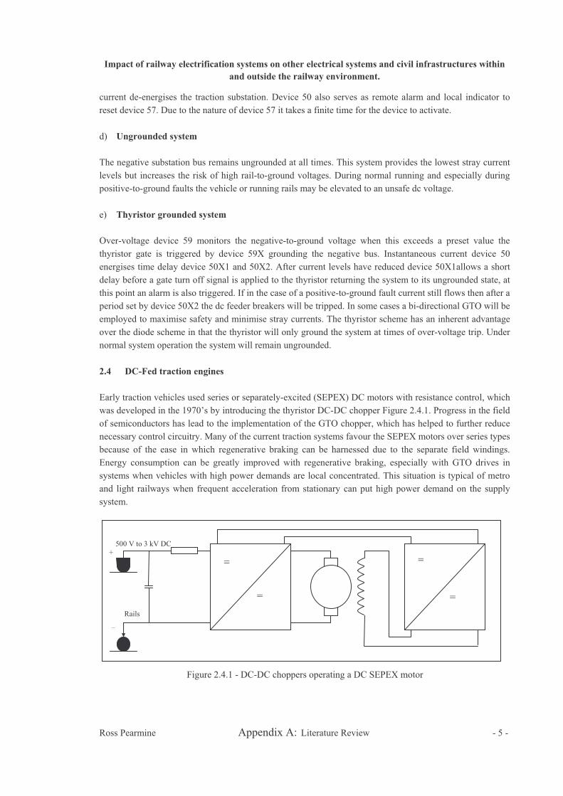
2.4 DC-Fed traction engines
Early traction vehicles used series or separately-excited (SEPEX) DC motors with resistance control, which was developed in the 1970’s by introducing the thyristor DC-DC chopper Figure 2.4.1. Progress in the field of semiconductors has lead to the implementation of the GTO chopper, which has helped to further reduce necessary control circuitry. Many of the current traction systems favour the SEPEX motors over series types because of the ease in which regenerative braking can be harnessed due to the separate field windings. Energy consumption can be greatly improved with regenerative braking, especially with GTO drives in systems when vehicles with high power demands are local concentrated. This situation is typical of metro and light railways when frequent acceleration from stationary can put high power demand on the supply system.
= =
500 V to 3 kV DC +
_Rails
Figure 2.4.1 - DC-DC choppers operating a DC SEPEX motor

Impact of railway electrification systems on other electrical systems and civil infrastructures within
and outside the railway environment.
Ross Pearmine Appendix A: Literature Review - 6 -
The DC-DC chopper can give rise to current harmonics in the supply, particularly when starts up currents in the order of 4 kA are drawn. These harmonic currents can both influence the signalling or communications network and degrade the incoming voltage from the Supply Company. The harmonics are greatest when the mark-space ratio of the chopper is 1:1 with the fundamental at the fixed chopping frequency. A low-pass filter at the power collection terminals is used to attenuate the harmonic content of the line current.
The development of the power thyristor in the 1970’s also lead to the application of induction motors operating from current-source inverter (CSI) systems, Figure 2.4.2 and Figure 2.4.3. These systems evolved into induction motors operating from a voltage-source inverter (VSI) when the fabrication of high power GTO became possible, Figure 2.4.4. The motors themselves can be fed from VSI which is both variable frequency and variable voltage or CSI which require a pre chopper to maintain a constant link current.
3 kV DC
Rails
VSI
Figure 2.4.4 – DC-DC chopper to 3 phase voltage source inverter operating an induction motor drive
750 V DC
Rails CSI
Figure 2.4.2 – DC-3 phase current source inverter operating an induction motor drive
750 V DC
Rails CSI
Figure 2.4.3 – DC-DC chopper to 3 phase current source inverter operating an induction motor drive
Impact of railway electrification systems on other electrical systems and civil infrastructures within
and outside the railway environment.
Ross Pearmine Appendix A: Literature Review - 7 -
VSIs operating from a DC source can tolerate large fluctuations in supply voltage with the exception of high voltage 3 kV lines where it is necessary to limit reverse voltage to the inverter power devices by use of a chopper. Voltage inverters can use a number of established techniques or combinations of techniques to ensure the correct power characteristics for traction are employed. Of these techniques pulse width modulation (PWM) and Quasi-square wave operations are common.
A CSI operating from a DC source requires constant current achievable from DC chopper with a duty cycle which matches the current demand. Thyristors are implemented in CSI circuits of this type in favour of GTOs devices because of their ability to withstand high reverse voltages.
New technologies are emerging thanks to developments in the transistor markets and IGBT or Integrated Gate Bipolar Transistor packs are now being implemented in four-quadrant converters. The IGBT has the significant advantage of high switching speeds (kHz - GHz) improving the shape of output waveforms, and also a reduction in energy consumption, cost and size.
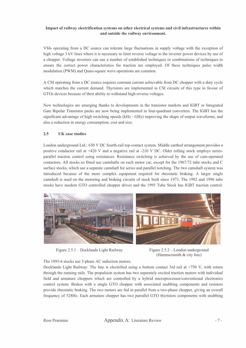
2.5 UK case studies
London underground Ltd.: 630 V DC fourth-rail top-contact system. Middle earthed arrangement provides a positive conductor rail at +420 V and a negative rail at -210 V DC. Older rolling stock employs series-parallel traction control using resistances. Resistance switching is achieved by the use of cam-operated contactors. All stocks so fitted use camshafts on each motor car, except for the 1967/72 tube stocks and C surface stocks, which use a separate camshaft for series and parallel notching. The two camshaft system was introduced because of the more complex equipment required for rheostatic braking. A larger single camshaft is used on the motoring and braking circuits of stock built since 1973. The 1992 and 1996 tube stocks have modern GTO controlled chopper drives and the 1995 Tube Stock has IGBT traction control.
The 1995-6 stocks use 3-phase AC induction motors. Docklands Light Railway: The line is electrified using a bottom contact 3rd rail at +750 V, with return through the running rails. The propulsion system has two separately excited traction motors with individual field and armature choppers which are controlled by a hybrid microprocessor/conventional electronics control system. Brakes with a single GTO chopper with associated snubbing components and resistors provide rheostatic braking. The two motors are fed in parallel from a two-phase chopper, giving an overall frequency of 528Hz. Each armature chopper has two parrallel GTO thyristors components with snubbing
Figure 2.5.1 – Docklands Light Railway Figure 2.5.2 – London underground (Hammersmith & city line)

Impact of railway electrification systems on other electrical systems and civil infrastructures within
and outside the railway environment.
Ross Pearmine Appendix A: Literature Review - 8 -
and smoothing. Each field power supply has two series connected GTO thyristors and a four thyristor reversing bridge with smoothing and snubbing components.
Railtrack: +750 V DC third rail top contact system, with return through the running rails; used in urban and suburban railway network in south-eastern zone. 3 phase induction motors with two VSI GTO inverters per driving car, blended regenerative/rheostatic braking with facility to blend with the air brake system. Designed with an ICMU (interference current monitoring unit).
Croydon Tramlink: +750 V DC direct overhead-line driven system, with return through the running rails. Drive system consists of two GTO pulse inverters DPU 251 plus microprocessor controlled drive-brake controller EFB 251 in conjunction with robust and maintenance free transverse, encapsulated, self cooled 3 phase asynchronous traction motors.
Midland Metro: +750 V DC direct overhead-line driven system, with return through the running rails.
Figure 2.5.3 – Class 465 750 V DC traction unit at Waterloo East
Figure 2.5.4 - East Croydon. Croydon Tramlink Figure 2.5.5 - Lodge Road. Midland Metro
Figure 2.5.6 - Sheffield Supertram Figure 2.5.7 - Manchester Metrolink

Impact of railway electrification systems on other electrical systems and civil infrastructures within
and outside the railway environment.
Ross Pearmine Appendix A: Literature Review - 9 -
Sheffield Supertram: +750 V DC direct overhead-line driven system, with return through the running railsTractive effort produced by the conventional Siemens monomotor design, driven by a chopper-controlled DC traction motor. Combined regenerative and rheostatic braking.
Manchester Metrolink: +750 V DC direct overhead-line driven system, with return through the running rails.On Phase I vehicles, traction is provided by four separately - excited DC motors, each motor group is fed from independently controlled choppers utilising gate turn off (GTO) thyristors. The separate field control is also provided on a per bogie basis, and this is achieved using four quadrant inverters with insulated gate bipolar transistor (IGBT) technology reducing the overall component count and weight. In the six new vehicles the motors are AC and utilise IGBTs. Electric braking is regenerative / rheostatic, with the energy being dissipated from naturally - cooled resistors mounted on the roof of the vehicle. A line filter performs three functions: it presents a low impedance source to the chopper and a high impedance to the alternative current voltage component in the overhead 750v supply. It also filters out chopper - generated ripple. The choppers are controlled by a microprocessor and operate at an interlaced chopping frequency of 600 Hz. This frequency does not deviate into signalling frequencies.
Tyne and Wear Metro: +1.5 kV DC overhead-line driven system, with return through the running rails. It is probably the last of the LRTs to use rheostatic current limiting. Traction system employs Gate Turn Off (GTO) chopper control.
2.6 Outline of DC traction simulation
Modeling is vital in the design process for a new railway, or the upgrade of an existing railway system. The modeling process can minimize the commercial risks on new projects or upgrades to existing railways due to mainly to interference. Modeling provides detailed information on the performance of the railway system and predictive evidence of compliance with railway and national standards (EMC, control of return currents and earthing). Many tasks in simulation are interrelated and manual calculations are laborious and are also highly susceptible to human error. To give a high degree of confidence the systems based on computer programs are being used in the area of railway power systems design. Computer-aided methods are necessary to aid engineers because of the complexity of the DC networks involved. Simulations will give confidence to the operational side of the business and minimize the risk associated with interference. Careful hazard analysis, simulation studies and design of the system will provide performance characteristics and mitigate, against incompatibility.
Figure 2.5.8 - Newcastle Tyne & Wear Metro

Impact of railway electrification systems on other electrical systems and civil infrastructures within
and outside the railway environment.
Ross Pearmine Appendix A: Literature Review - 10 -
2.6.1 Review of existing software
To examine the effect of a running train service in terms of timetables and signalling sophisticated simulation software has been developed by many rail companies. The British Rail system is called OSLO (Overhead System Loading) and Balfour Beatty uses its RAILPOWER program, whilst GEC-ALSTHOM software is believed to be based on software developed at Birmingham University.
A well developed simulation suite developed by Mellitt et al. (1978) at University of Birmingham utilizes a two part, three stage simulator for DC railways based around train movement and power-network simulation. The suite was specifically developed for simulation studies with chopper drives and regenerative braking although it allows more than energy consumption to be modeled. The simulator makes piecewise calculations over the whole track considering one section at a time. The program uses data arrays to hold information on all sections and all trains between network power calculations. The simulator considers the dc traction motor in one of four operational modes according to tractive effort supplied and models the train as an equivalent circuit according to this mode. The program as explain earlier operates in three stages:
Movement simulator (part A); establishing the train mode
Power network solution; simulating node voltages
Movement simulator (part B); updates train position and velocity
T ST
TT
S T S
TT
T S
I1d I3dI2
I2uI1u I3u I5u
I4d I5d
I4u
I7d
I6u
I6d
I7u
R1 R4 R3 R4
r1u r2u r3u r4u’’
r4u r5u r6u r7u
r1d r2d r3d r4d’’ r4d r5d r6d r7d
R1 R2R3 R4
R1 R2 R3 R4
T S
TT
T S
I5u
I4d
’I5d
’
I4u
’
I7d
’
I6u
’
I6d
’
I7u
’
R3
’R4
’
r4u’ r5u
’r6u
’r7u
’
r4d’ r5d
’r6d
’r7d
’
R3
’R4
’
R3d’ R4
’
V V V V
V4
’V3’
E1 E1 E1 E1
E1
E2E3
E4
E3u
’
E4u
’
Figure 2.6.1 – Simplified power network with braches

Impact of railway electrification systems on other electrical systems and civil infrastructures within
and outside the railway environment.
Ross Pearmine Appendix A: Literature Review - 11 -
Jinzenji and Sasaki (1998) base a DC simulator on train behavior, realizing that trains are restricted by signal conditions and passengers. A block system is used to model train movement on the lines, with a simple equivalent circuit to model the system electrically. The simulator attempts to mimic field data in terms of temporal systems loading if not in magnitudes.
Software developed by Ho et al.(2002) utilises a set of efficient algorithms in a power network simulator. The simulator assumes all conductive components are linear in nature and the feeder substations are a simple voltage source with series resistance. The substation is replaced with a resistive load when regenerative braking is harnessed. The traction systems are also modelled as a V-R system but values of both characteristics are variable with speed and the units operating mode. The software formulates and solves a matrix equation for the electrical circuit using nodal analysis on the system Figure 2.6.1.
A set of software algorithms are presented by Talukdar and Koo (1977) which are developed for specific use in the railway sector for load flow calculations. Conventional power systems analysis tools cannot be applied to the railway network because of its mobile loads and alternative system frequencies that the system may develop. The work is based on the proposal that traction vehicles do not move fast enough to cause transient effects due to their constantly changing velocities on the supply system. The power network can be assumed to simply change states as power demands alter. A representation of the electrical performance can thus be created from a series of load-flow samples taken in the period of interest. The paper provides methods for the solution of embedded DC traction system in an AC network.
A simulation package that includes regenerative braking was developed at Brunel University for Balfour Beatty by Cai [34] and [35]. The software solves the DC-load-flow problem using iterative techniques based on linear, bi-lateral and lumped circuit parameters. The software developed is adapted for use in both the AC and DC traction environments and is based around the normal two stage program, simulating both movement and also the power network.
Daniels and Jacimovic (1983) develop a design stage power network simulator for use in evaluating the requirements of the utility supply, working voltages, component ratings and harmonic performance. Developed by the International Engineering Company, inc. the package executes a TSP and LFP program to calculate system conditions (see Figures 2.6.2 and 2.6.3).
The result from the LFP is temporal snapshot of: 1. Substation AC and DC volts, amps and watts vs. time
Track Data (gradient and
curvature)
Speed
Train
Operation
Train Simulator
Train LocationTime PowerEnergy Speed
Speed Limit Acceleration
Train Resistance
Tractive EffortVoltage
Feeding Diagram
Network Impedance
Train Schedule
TSP Results
Auxiliary Load
Catenary Data
Voltage at DC bus
Branch DC current
S/S DC current
AC current
AC source voltage
Energy
Power
Load
Flow
Figure 2.6.2 – Train simulation program (TSP) Figure 2.6.3 – Load flow program (LFP)

Impact of railway electrification systems on other electrical systems and civil infrastructures within
and outside the railway environment.
Ross Pearmine Appendix A: Literature Review - 12 -
2. DC amps at feeders and catenary vs. time 3. Utility AC voltage fluctuation vs. time 4. AC and DC rms power and currents (peak, off-peak and combined) vs. time 5. Catenary and rail potential vs. distance 6. Energy demand
This data can be saved to a system file or stored graphically and in tabular form in data files.
A program developed by Borwn Boveri (1979) is another design stage simulator for DC traction systems. The program operation is limited to a relatively simple model of a single track but it does allow for a traffic schedule to be implemented on the line. The model calculates line voltages and currents at any point in the schedule and any distance along the track. The program also allows regenerative braking to be employed and so can evaluate the energy levels of the system.
3. AC RAILWAY ELECTRIFICATION
3.1 AC traction lines
For 25 kV networks at 50 Hz supply is directly fed from the electrical utilities via a single-phase transformer substation. Adjacent sections of track are usually supplied from alternate utility phases to keep an equal loading of the three-phase network. The 15 kV, 16 Hz system is more complicated requiring special generators or frequency converter circuits to supply the require feed.
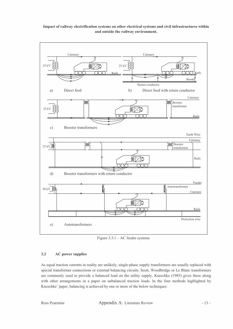
Using a simple transformer arrangement as in Figure 3.3.1a and 3.3.1b is the most economically viable method of supply. In the case of figure 3.3.1a a direct connection to the rails and catenary is made via transformer secondary windings this. This has the disadvantage of large losses, high touch potentials and stray currents that interfere with telecommunications and increase erosion of local metallic pipework. Introducing a cross-bonded return conductor to the system provides a lower impedance path for return currents and its screening effect can also help reduce interference. A more capital-intensive method to reduce interference of traction currents is the addition of booster transformers as shown in Figure 3.3.1c and 3.3.1d. These are unity transformers connected across sectionalized catenary and rails, at intervals of 3-4 km. Return current is forced to flow from the rails and earth into the transformer secondary to equalise the ampere-turns of the primary circuit. In most cases a parallel conductor arrangement is preferred as in figure 3.3.1d to carry the return current. In high voltage AC rail networks the line impedance constitutes most of the total feeding impedance which at power frequency is a result of both physical layout and material properties.
Using an autotransformer system (Figure 3.3.1e) allows an increase in the substation spacing because of the higher transmission voltage involved. The autotranformer is connected across the catenary and an auxiliary feeder with the rails connected to an intermediate point. For 25 kV systems the autotransformers are center-tapped with a unity ratio and a 50 kV supply. A train draws a current, double that of the traction current, through two adjacent autotransformers. Current flows through the autotransformers so that the ampere-turn balance is kept. In an ideal system no current flows along unoccupied rails and so the maximum earth current occurs in-between supplying autotransformers and is a minimum at these transformers.
Impact of railway electrification systems on other electrical systems and civil infrastructures within
and outside the railway environment.
Ross Pearmine Appendix A: Literature Review - 13 -
3.2 AC power supplies
As equal traction currents in reality are unlikely, single-phase supply transformers are usually replaced with special transformer connections or external balancing circuits. Scott, Woodbridge or Le Blanc transformers are commonly used to provide a balanced load on the utility supply, Kneschke (1985) gives these along with other arrangements in a paper on unbalanced traction loads. In the four methods highlighted by Kneschke’ paper, balancing is achieved by one or more of the below techniques:
Rails
25 kV =
Catenary
=
Catenary
Rails
25 kV
Bonds
Return conductor
Rails
25 kV =
Catenary
Booster transformer
Earth Wire
Rails
25 kV
=
Catenary Booster transformer
Rails
50 kV
=
Catenary
Feeder
Protection wire
Autotransformer
Figure 3.3.1 – AC feeder systems
a) Direct feed b) Direct feed with return conductor
c) Booster transformers
d) Booster transformers with return conductor
e) Autotransformers
Impact of railway electrification systems on other electrical systems and civil infrastructures within
and outside the railway environment.
Ross Pearmine Appendix A: Literature Review - 14 -
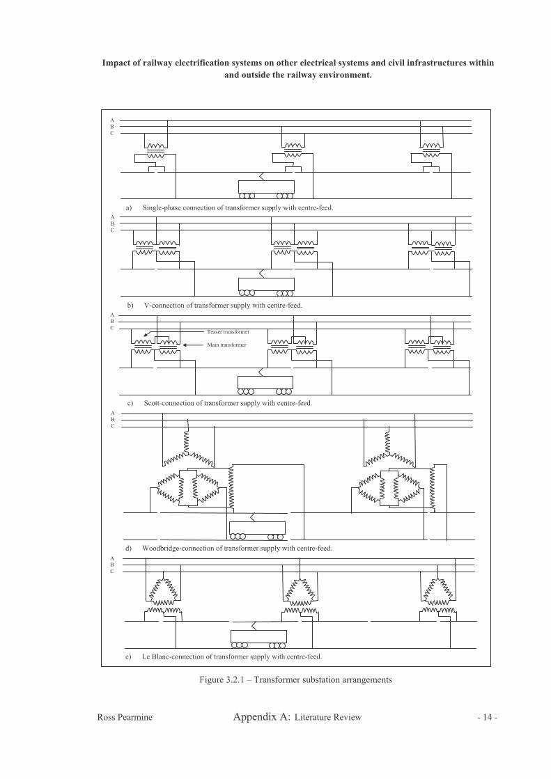
Figure 3.2.1 – Transformer substation arrangements
b) V-connection of transformer supply with centre-feed.
a) Single-phase connection of transformer supply with centre-feed.
c) Scott-connection of transformer supply with centre-feed.
d) Woodbridge-connection of transformer supply with centre-feed.
e) Le Blanc-connection of transformer supply with centre-feed.
ABC
ABC
ABC
ABC
ABC
Teaser transformer
Main transformer
Impact of railway electrification systems on other electrical systems and civil infrastructures within
and outside the railway environment.
Ross Pearmine Appendix A: Literature Review - 15 -
Inherent balancing - successive transformers along the supply line are assigned to alternate phases of the supply network. This is achieved through the sectionalising of the catenary shown in Figure 3.2.1a.
Local balancing - two-single phase, three-to-two phase and three-phase transformers. Balance is achieved by equally loading the local the supply network at the substation, Figures 3.2.1b through e.
External balancing - static or rotary balancing equipment.
Three-phase to single-phase converters - rotary or static converters.
The relative unbalance factor for the V-connected transformer in Figure 3.2.1b compared to that of a single-phase type is 0.5 for the same load. Of the three-two phase types, Scott-connected transformers consist of two sets of windings. The main winding is connected across two supply phases and is centre-tapped, the teaser winding connects the tap point to the remaining phase. The transformer secondary winding voltages
are 3⁄2. degrees out of phase from each other. The main winding is formed from the desired turns ratio,
while the teaser winding is a multiple of times the ratio. In the Woodbridge-connection two secondary
voltages are supplied, which are again degrees out of phase but for this arrangement the voltages are unequal. This lower voltage must be raised to match the traction voltage. The secondary windings do not have a common point and as such it is necessary to connect each winding to a different track or to the same track with sectionalised by insulated rail joints. The Le Blanc transformers are similar to Scott types, and the two can be used together in double end-feed systems.
Three-phase transformers can be used for AC traction power supply but they do not produce balance loading of the utility side in symmetrical or asymmetrical arrangements.
In cases where sufficient balancing cannot be accomplished by the choice of transformer connection the use of external equipment can be employed. Static equipment achieves balance of the utility side by the use of capacitor and inductor elements; the system components can also be used for power factor correction. Rotary balancing equipment such as synchronous condensers or induction motors act as a sink for negative sequence currents of the three-phase system. Three-to-two phase converters can be used in situation when no other technique achieves the required balance characteristics. Here a three-phase motor draws balanced current from the utility and can be used to supply torque to a single-phase generator. Static converters can also be employed which utilise semiconductor devices, but they have the draw back of introducing current harmonics into the supply system.
Low power factor is a particular problem in long track sections with single-end feed supply intensified by the use of electronic drives. Power factor can be broken down into two constituent parts displacement factor and distortion factor. The first is governed chiefly by impedance of the traction line, and the later arises due to high levels of harmonics in the line current. Rectifier locomotives can have power factors ranging as low as 40 % during initial acceleration, correction is needed to satisfy specifications imposed by the supply utility. Normally incoming feeders are connected to HV or EHV grid voltages to minimize the effects of harmonics on the utility supply.
Low power factor is a particular problem in long track sections with single-end feed supply intensified by the use of electronic drives. Power factor can be broken down into two constituent parts displacement factor and distortion factor. The first is governed chiefly by impedance of the traction line, and the later arises due to high levels of harmonics in the line current. Rectifier locomotives can have power factors ranging as low as 40 % during initial acceleration, correction is needed to satisfy specifications imposed by the supply

Impact of railway electrification systems on other electrical systems and civil infrastructures within
and outside the railway environment.
Ross Pearmine Appendix A: Literature Review - 16 -
utility. Normally incoming feeders are connected to HV or EHV grid voltages to minimize the effects of harmonics on the utility supply.
Semi-conductor controlled traction equipment and magnetic saturation in transformers and machines can cause resonance in the network creating high frequency currents. These currents can cause increased heating in equipment windings, overcurrents in line capacitors, undervoltages at locomotive pantographs and line overvoltages that exceed safe levels. These effects pose more serious problems in traction systems because of the low impedance of the lines; typically an inductance of 1.33 mH.km-1, capacitance of
0.011 F.km-1, and resistance of 0.17 .km-1 which produce resonance at 1 kHz. Traction loads are also high in comparison with the line fault levels, a 10 MW substation may feed a long line with a fault level of 40MW at its termination. Lastly input filters on locomotives interact with the line reactance which may have adverse effects on the problems highlighted above.
3.3 Feeding arrangements
The function of the feeder station, intermediate track sectioning cabin and mid-point track sectioning cabin are to control distribution of the supply to the track. The mid-point cabin as its name suggests is sited between two adjacent feeder stations, whilst the intermediate cabin is approximately halfway between the feeder and mid-point cabin. The mid-point cabin provides electrical isolation for overhead line equipment, neutral sections and track paralleling for the 25 kV systems. The intermediate cabins provide similar functions to the mid-point cabins with the exception tat they cannot terminate feeding sections, both types of cabin increase the systems resilience during loss of supply.
As with DC systems the feeding arrangements can be single-end, double-end or center fed dependant on circuit conditions.
3.4 AC-Fed traction engines
At the introduction of the 25 kV electric supply system, locomotives that used rectifier devices became introduced into service. Figure 3.4.1 shows a typical schematic of the circuitry. It is more common to find the rectifiers in these circuits to be of the semi-controlled bridge type rather than full-bridge. This is due to lower costs and higher operating performance in terms of power factor and armature harmonics. The basic
Feeder Station FeederStation
Intermediate Track Sectioning
Cabin
Mid-point Track Sectioning
Cabin
Intermediate Track
SectioningCabin
CircuitBreaker (NO)
CircuitBreaker (NC)
NeutralSection
132/25 kV Transformer
SectionOverlap
Figure 3.3.1 – Typical 25 kV ’classic’ Feeding section

Impact of railway electrification systems on other electrical systems and civil infrastructures within
and outside the railway environment.
Ross Pearmine Appendix A: Literature Review - 17 -
semi-controlled bridge cannot utilise regenerative braking but this is not usually a problem in long distance lines.
Voltage harmonics created by using the semi-controlled method can be calculated by the use of the Fourier series with the worst voltage harmonic being the second. This harmonic is at a maximum when the firing
angle = /3 radians. Approximating the input current as a rectangular waveform allows assessment of the circuit current harmonics, due to the large inductance this is a realistic assumption. The semi-controlled bridge can be shown to reduce the armature current harmonics (beneficial to reduce motor torque ripple) but at a cost of increasing the line harmonics. One method employed to reduce the line harmonics is to switch in more series rectifier circuits. Typically a second bridge with a centre tapped transformer assists in the conduction at half to full supply voltage.
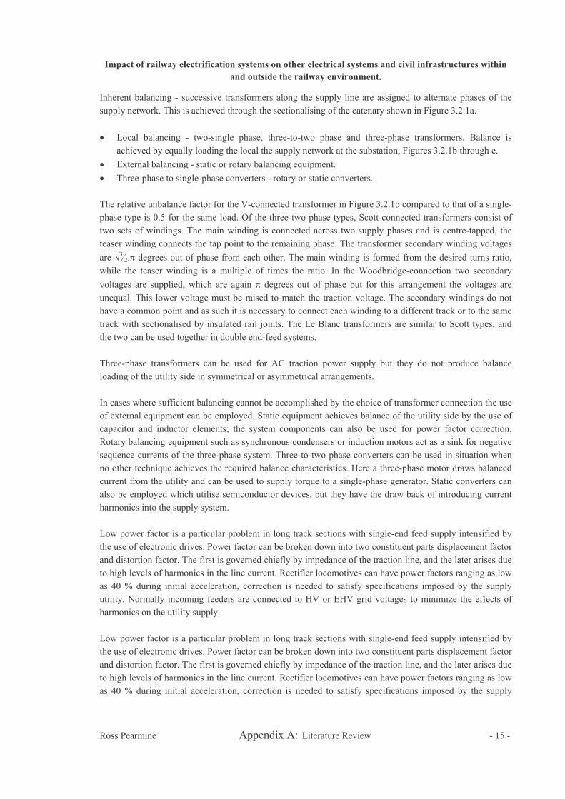
In all AC-fed VSI and CSI drives Figure 3.4.2, Figure 3.4.3 and Figure 3.4.4 an AC-DC converter is required to supply the DC link. Commonly a PWM four-quadrant converter is employed which allows for regenerative braking. This type of converter mimics the action of a variable ratio transformer drawing a
25 kV 50 Hz
Rails
CSIPulse converter
Figure 3.4.2 – AC-DC pulse converter to 3 phase current source inverter operating an induction motor drive rotor, DC-DC chopper feeding motor field winding
=
=
25 kV 50 Hz or 15 kV 16 Hz
Rails
Figure 3.4.1 – AC-DC Rectifier operating a DC SEPEX motor
Impact of railway electrification systems on other electrical systems and civil infrastructures within
and outside the railway environment.
Ross Pearmine Appendix A: Literature Review - 18 -
variable sinusoidal voltage and current at the line frequency. A series filter at twice the supply frequency is required to filter the AC component of the output voltage and the line inductance improves output current ripple. By the careful choice of modulation strategy it is possible to greatly reduce system current harmonics.
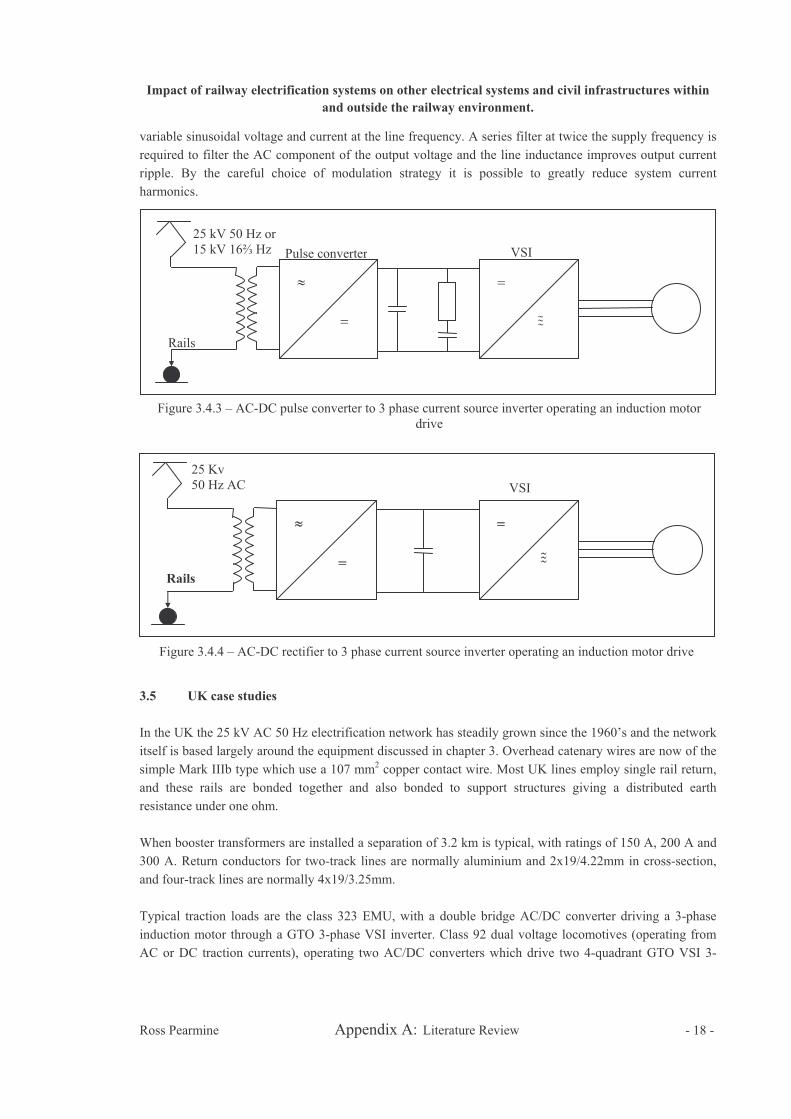
3.5 UK case studies
In the UK the 25 kV AC 50 Hz electrification network has steadily grown since the 1960’s and the network itself is based largely around the equipment discussed in chapter 3. Overhead catenary wires are now of the simple Mark IIIb type which use a 107 mm2 copper contact wire. Most UK lines employ single rail return, and these rails are bonded together and also bonded to support structures giving a distributed earth resistance under one ohm.
When booster transformers are installed a separation of 3.2 km is typical, with ratings of 150 A, 200 A and 300 A. Return conductors for two-track lines are normally aluminium and 2x19/4.22mm in cross-section, and four-track lines are normally 4x19/3.25mm.
Typical traction loads are the class 323 EMU, with a double bridge AC/DC converter driving a 3-phase induction motor through a GTO 3-phase VSI inverter. Class 92 dual voltage locomotives (operating from AC or DC traction currents), operating two AC/DC converters which drive two 4-quadrant GTO VSI 3-
25 kV 50 Hz or 15 kV 16 Hz
Rails
VSIPulse converter
Figure 3.4.3 – AC-DC pulse converter to 3 phase current source inverter operating an induction motor drive
25 Kv 50 Hz AC
Rails
VSI
Figure 3.4.4 – AC-DC rectifier to 3 phase current source inverter operating an induction motor drive

Impact of railway electrification systems on other electrical systems and civil infrastructures within
and outside the railway environment.
Ross Pearmine Appendix A: Literature Review - 19 -
phase inverters. Class 332 EMU operating from three parallel 4-quadrant-input AC/DC converters which drive a 3-phase induction motor via two parallel IGBT PWM inverters.
3.6 Review of existing AC traction simulation software
Hsi et al. (1999) present an AC simulator which provides a multi-train algorithm for the solution of power flow problems. The paper solves system power flows by decoupling the autotransformer currents into two separate currents the main current and auxiliary current Figure 3.6.1. Treating the upper and lower AT coils separate means that equivalent circuits can be determined for main and auxiliary train currents. The magnitude of the train current supplied by each AT can be found from its inverse aggregate series impedance. Once the currents are quantified the train voltage can be found by considering the voltage drop across each section. For multiple trains the same half-circuit technique can be used and the resulting main and auxiliary currents can be superimposed together. The software developed in this example can solve problems with both constant current and constant power train models.
Hill and Cevik (1993) adopt a similar technique to that of Hsi with the addition of modelling a double-end feeding arrangement. The simulator was originally developed for predicting the voltage regulation characteristics of an AC autotransformer system. Current supplied by each AT is assumed on a proportional basis of the train position on the track, the AT closer to the train supplying a higher percentage of the traction current. The package delivers a time varying reading of catenary and rail potentials, and also a
Rails
50 kV
=
Catenary
Feede
Autotransformer
Zs
AT2AT1
Figure 3.6.1 – Current shared amongst autotransformers
Main current
Auxiliary current
AT1AT2
Zrail
Zcatenery
Itrain
Figure 3.5.1 – Class 332 EMU: Heathrow Express
Figure 3.5.2 – Class 323 EMU
Impact of railway electrification systems on other electrical systems and civil infrastructures within
and outside the railway environment.
Ross Pearmine Appendix A: Literature Review - 20 -
voltage history for trains during each run. It provides a design stage tool enabling substation to be place for optimum train and network performance.
Developed at Birmingham University Chan et al. (1989) propose a piece by piece model of the railway network. The traction motor and converter are both modelled by a set of known equations and a different set of equations exists for the three modes of train operation employed. For the power network each feeding section is considered individually and as a multi-conductor system. System currents are derived from a mesh equation involving admittance and impedance matrices and voltages similarly can be derived from a nodal equation.
Further work from Birmingham University lead to Mellitt et al. (1990) presenting a comprehensive technique to calculate induced voltages in line-side cables. The tool also allows earth current distribution for AT and BT systems to be calculated. The program itself originated because of psophometric voltage limits imposed by the CCITT particularly on lineside telephone cables. The paper compares the accuracy of computer-based approaches with more antiquated mathematical estimates. The software is based around a sectionalized multi-conductor track recorded in terms of impedance and admittance matrices.
Pilo et al. (2000) have developed a two part simulator that employs a traffic and AC electrical simulator which provide isolated data that feed into program sub routines. The traffic simulator calculates train motion in terms of distance and time by Newton’s second law. A line parameters routine calculates impedance and admittance matrices and then load flow is solved using the Newton-Raphson method. The tool was developed further to calculate unbalanced voltages from direct and inverse sequence voltages, step and touch voltages from equivalent impedances allowing voltages to be obtained by solving nodal equations and induced voltages in parallel lines.
4. CIRCUIT PARAMETERS
In order to simulate any of the railway networks we must have a model for all the basic constituent components. These include conductor rails, overhead pantographs, earth resistance, traction drives, substation feeding and many other items. Some specific components have already been considered in a number of papers.
4.1 Rail impedance
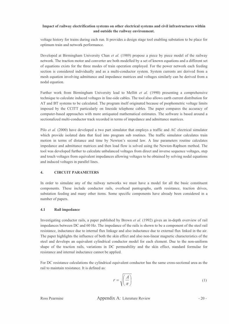
Investigating conductor rails, a paper published by Brown et al. (1992) gives an in-depth overview of rail impedances between DC and 60 Hz. The impedance of the rails is shown to be a component of the steel rail resistance, inductance due to internal flux linkage and also inductance due to external flux linked in the air. The paper highlights the influence of both the skin effect and also non-linear magnetic characteristics of the steel and develops an equivalent cylindrical conductor model for each element. Due to the non-uniform shape of the traction rails, variations in DC permeability and the skin effect, standard formulae for resistance and internal inductance cannot be applied.
For DC resistance calculations the cylindrical equivalent conductor has the same cross-sectional area as the rail to maintain resistance. It is defined as:
(1) A
r

Impact of railway electrification systems on other electrical systems and civil infrastructures within
and outside the railway environment.
Ross Pearmine Appendix A: Literature Review - 21 -
Figure 4.1.1 – Equivalent cylindrical conductor model for rails.
h
0.45h
r
For high-frequency AC resistance calculations above 12 Hz, due to the predominant action of skin effect the equivalent conductor must have a circumference that is equal to the perimeter of the rail. Therefore:
(2)
The paper also attempts to model the inductive properties of the rails but without satisfactory results. It concludes that although the external inductance can be calculated assuming a circular boundary equal to the perimeter of the rail, the internal inductance cannot be modelled correctly by a cylindrical conductor. To
determine the internal inductive properties of the rail two methods based around the same technique have been employed in the past. The first technique is that used by Carpenter and Hill (1993), Hill and Carpenter (1993) and Carpenter and Hill (1991) and involves finite element analysis. The technique involves constructing and elemental net base around the rail shape. This net is then used to perform an axisymmetric static and dynamic electromagnetic analysis. The internal inductance can then be obtained by evaluating the stored energy in the material (3) and also the resistance can be found from (4).
(3)
(4)
Silvester [14] describes this approach as determining the minimum energy state through the minimisation of a specific function derived from the Helmholtz equation (5).
(5)
.2
Pr
BH dI
.2
2
S.1
2S
sJ
IR
JAA ....22

Impact of railway electrification systems on other electrical systems and civil infrastructures within
and outside the railway environment.
Ross Pearmine Appendix A: Literature Review - 22 -
To interpret the irregular shape of the rails as a circular conductor for inductance calculations the geometric mean distance or GMD must be evaluated. This is achieved by evaluating equation (6), which is establishing the GMD of the rail from itself by assessing the effect of a rail composed of many filaments.
(6)
Assuming that all current flows within the skin depth an equivalent conductor annulus must be calculated and converted to a solid cross-section for modeling. This can be achieved through equation (7).
(7)
The second technique is shown by Lucas and Talukdar (1978), Barr (1991) and also by Wang (1999) and uses a coupled-inductance theory for the modelling of the rail. Slivetser (1966) introduced the basic principle; the theory assumes that the rail is enclosed in a thin cylindrical sheath of radius r in which return current flows, similar to Figure 4.1. The return current is uniformly distributed over the sheath surface and allows not only a defined path for this current but also ensures current distribution in the rail is not affected by proximity effect. The rail cross section is divided into n sub-conductors.
The resistance per unit length then becomes (8) and the mutual inductance between the ith and jth sub-conductor is given by (9).
(8)
(9)
If i=j then the GMD is substituted as distance d; this can be approximated by their center-to-center distance.
If i j then the GMR is substituted for d and is obtained from a quadruple integral, Figure 4.1.2 shows the
GMR for most common conductor shapes and is taken from a paper by Aguet and Morf (1987).
When the self and mutual inductance for all individual sub-conductors are derived they can be entered into an inductance matrix as highlighted in (7) and a resistance matrix (8) can also be constructed. The voltage current relationship for the conductor can be written in matrix form as (9) where the voltage vector V is identical for all the sub-conductors as shown in Figure 4.1.3.
m m
mmAG
)ln(.ln
7788.0circleofGMD
annulusofGMD
A
nr
.
ij
ijd
aln.
.20

Impact of railway electrification systems on other electrical systems and civil infrastructures within
and outside the railway environment.
Ross Pearmine Appendix A: Literature Review - 23 -
V
I
I
I
Il13
l12
l23
l13
l22
l33
Figure 4.1.3 – Coupled-circuit model of sub-conductors
r
r
r
(7) (8)
(9)
Letting the voltage equal some arbritory value say 1 equation 9 then has only one unknown matrix I , so the solution becomes the inverse impedance matrix [Z]-1. This can be solved by computer program using the
LU decomposition technique. For frequency-dependant values of resistance and inductance the sum of the individual currents in all sub-conductors is representative of the total current in the conductor.
External inductance due to flux linkage in the air external of the rail can be calculated from the geometrical features of the track layout. The flux boundary between internal and external inductance is given as that of the equivalent conductor radius derived from eqn. (1) acting at a centre that is 0.45 of the rail height above the base.
4.2 Earth impedance
The conductivity of the soil is a significant characteristic when modelling railway or in fact any earthed electrical systems. Not only does the parameter affect ground-return current magnitudes but also significantly influences rail admittance. A paper by Hill et al. (1999) collates much information on track
r
r
r
00
0
0
00
R
iji
j
1
2221
11211
L
a
s 2r
2r
2r1 2r2
a
a
a
SrrGMR .4394.0.7788.0)4
1exp(.
rGMR
221
22
1
241
22
21
42
2 )(
)]ln(4
3[.
4
rr
r
rrrr
r
r
GMRLn
aaGMR .22313.0)2
3exp(.
aGMR .44705.0
aGMR .578.0
Figure 4.1.2 – GMR of common conductor shapes
]].[[]].[.[]].[[][ IZILIRV j
Impact of railway electrification systems on other electrical systems and civil infrastructures within
and outside the railway environment.
Ross Pearmine Appendix A: Literature Review - 24 -
parameters and especially those concerning soil conductivity. Table 1 gives a summary of the papers findings in relation to practical ground conductivity levels across a selection of countries including the UK.
Location Ground Topology Conductivity Range
Sweden Rock 0.01 mS.m-1 minimum 0.4 mS.m-1 nominal
Poland Alluvial 3.3-77 mS.m-1
UK Rubble stone 20-25 mS.m-1
France General 10 mS.m-1
Europe General 20-40 mS.m-1
USA Coastal region: poorly drained
0.057-4.12 mS.m-1
4.3 Traction drives
In order to electrical characteristics of traction units it is necessary to obtain a mathematical relationship between the tractive effort supplied by the motor and its voltage. This model can then be used to provide an accurate electrical model for introduction into a power network simulation.
Tractive effort developed by the traction engine mainly depends on the train operation and can either be constant or speed and voltage dependent. Complications develop due to lack in standardisation and the possibility of DC motor or AC induction motor drive systems, both systems are considered.
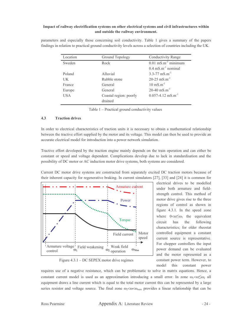
Current DC motor drive systems are constructed from separately excited DC traction motors because of their inherent capacity for regenerative braking. In current simulators [27], [33] and [24] it is common for
electrical drives to be modelled under both armature and field-strength control. This method of motor drive gives rise to the three regions of control as shown in figure 4.3.1. In the speed zone
where 0 1 the equivalent
circuit has the following characteristics; for older rheostat controlled equipment a constant current source is representative. For chopper controllers the input power demand can be evaluated and the motor represented as a constant power term. However, to model this constant power
requires use of a negative resistance, which can be problematic to solve in matrix equations. Hence, a
constant current model is used as an approximation introducing a small error. In zone 1 2 all
equipment draws a line current which is equal to the total motor current this can be represented by a large
series resistor and voltage source. The final zone 2 max provides a linear relationship that can be
Table 1 – Practical ground conductivity values
Armature current
Power
Torque
Field current Motor speed
Weak field operation
Field weakeningArmature voltage control
Figure 4.3.1 – DC SEPEX motor drive regimes
Max

Impact of railway electrification systems on other electrical systems and civil infrastructures within
and outside the railway environment.
Ross Pearmine Appendix A: Literature Review - 25 -
modelled by a resistor and voltage source that are both speed dependent. If regenerative braking is employed a straightforward constant power circuit can be used involving a voltage source and series resistor.
Changes in recent technologies as highlighted in previous sections have allowed the more appropriate three-phase induction motor to be used in traction applications. Characteristics of the induction motor over the traction duty cycle are given in Figure 4.3.3. Mellitt and Mouneimne (1988) have provided new methods in the electrical representation of AC inverter drive systems for traction applications.
The induction motor requires both stator supply frequency and voltage to be control for efficient
motoring. Zone 1 2 is
analogous to the armature voltage control in DC motors and so typical representation is as Figure 4.3.2a. IT can be deduced from the solution of equation 10. Again
zone 2 3 bears very similar
resemblance to the field weakening shown in DC motors. A simple constant current representation provides an applicable model. In zone
3 Max the drive operates
with constant input impedance. As both the slip and stator supply frequency are constant all motor circuit components are also constant.
(10)
1000
V=1000.IT
R= -(VT)2/P
V=2.VT V( ) V=2.VT
I( ) R=VT2/P
a) Armature voltage control - Constant
current
b) Field weakening - Constant power
c) Weak field mode a) Braking - Constant current
Figure 4.3.2 – Motor equivalent circuits
StatorCurrent
Terminal voltage
Torque
Motor speed
Reduced power
Constant power Constant flux
Figure 4.3.3 – Three-phase induction motor drive regimes
Max
Startup
Machineslip
i
mfTTTE
E
ZIRIVIP
cos...3..
212

Impact of railway electrification systems on other electrical systems and civil infrastructures within
and outside the railway environment.
Ross Pearmine Appendix A: Literature Review - 26 -
4.4 Motion simulation
In order so model train movement satisfactorily a Newtonian based equation is needed which relates force mass and acceleration. The following outlines the train resistance formula that can be used for load modelling calculations and simulations. The resistance for train movement on straight and level track can be determined, as proposed by W.J. Davis, as an empirical expression of the form:
(11)
For standard gauge (1435mm separation) railways the formulae listed in Association of American Railways (AAR) recommended practice RP-548 can be used.
The predominant but not exclusive contributors to the and coefficients are journal resistances, rolling rotational resistance and track resistance. Coefficient consists mainly of flange friction, flange impact, wave action of rail and the wheel to rail rolling resistance. Coefficient is composed mainly of head end wind pressure, skin air friction on the side of the train, rear air drag, air turbulence between vehicles and yaw angle of constant wind.
The total train resistance on a level tangent track is the sum of train resistances. When gradients and curves are involved the resistance for the portion of the train length on the curve or gradient is added to the total train resistance on level tangent track to produce a complete train resistance.
As previously stated the formula as listed in AAR RP-548 for locomotive resistance is used:
Coefficient Coefficient Coefficient Coefficient Locomotive resistance .00637 35.833 0.0254 0.0034 Carriage resistance .00637 89.582 0.0127 0.0073
The grade or gradient is a measure of the longitudinal inclination of railway track. To determine the grade resistance of an entire train:
(12)
Alternatively grade can be expressed as a percentage, then the resistance can be determined by multiplying the percentage value by a factor of ten to express the resistance in kg/t e.g. 1.67% grade:
(13)
Curve resistance is substantially contributed to by the flange contact to rail of the outer leading wheel of a bogie and the slip/slide over the railhead during curving of the two wheels on the same fixed axle. The sharper the curvature the higher the resistance of the portion of the train that is on the curve. The value of curve resistance is calculated in terms of kg/tonne by:
(14)
The tractive effort required to accelerate or the braking force to decelerate a train is calculated by multiplication of the train mass/inertia with the acceleration:
2....... TtTaaaTT vAvnnnmR
gmR Tg ..60
1000
gmR Tg .).67.110(
c
cr
R24.15
sin.4567.6 1
.. TTa maF
Table 2 – Coefficient values based on AAR RP-548
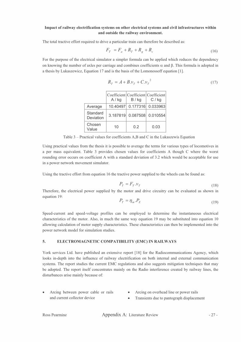
Impact of railway electrification systems on other electrical systems and civil infrastructures within
and outside the railway environment.
Ross Pearmine Appendix A: Literature Review - 27 -
The total tractive effort required to drive a particular train can therefore be described as:
(16)
For the purpose of the electrical simulator a simpler formula can be applied which reduces the dependency
on knowing the number of axles per carriage and combines coefficients and This formula is adopted in a thesis by Lukaszewicz, Equation 17 and is the basis of the Lomonossoff equation [1].
(17)
CoefficientA / kg
CoefficientB / kg
CoefficientC / kg
Average 10.40497 0.177316 0.033963
StandardDeviation
3.187819 0.087508 0.010554
Chosen Value
10 0.2 0.03
Using practical values from the thesis it is possible to average the terms for various types of locomotives in a per mass equivalent. Table 3 provides chosen values for coefficients A though C where the worst rounding error occurs on coefficient A with a standard deviation of 3.2 which would be acceptable for use in a power network movement simulator.
Using the tractive effort from equation 16 the tractive power supplied to the wheels can be found as:
(18) Therefore, the electrical power supplied by the motor and drive circuitry can be evaluated as shown in equation 19:
(19)
Speed-current and speed-voltage profiles can be employed to determine the instantaneous electrical characteristics of the motor. Also, in much the same way equation 19 may be substituted into equation 10 allowing calculation of motor supply characteristics. These characteristics can then be implemented into the power network model for simulation studies.
5. ELECTROMAGNETIC COMPATIBILITY (EMC) IN RAILWAYS
York services Ltd. have published an extensive report [18] for the Radiocommunications Agency, which looks in-depth into the influence of railway electrification on both internal and external communication systems. The report studies the current EMC regulations and also suggests mitigation techniques that may be adopted. The report itself concentrates mainly on the Radio interference created by railway lines, the disturbances arise mainly because of:
Arcing between power cable or rails and current collector device
Arcing on overhead line or power rails
Transients due to pantograph displacement
cgTaT RRRFF
2.. TTT vCvBAR
Table 3 – Practical values for coefficients A,B and C in the Lukaszewis Equation
TTT vFP .
EmT PP .

Impact of railway electrification systems on other electrical systems and civil infrastructures within
and outside the railway environment.
Ross Pearmine Appendix A: Literature Review - 28 -
Interactions of power contacts, wheel-to-rail and rail-to-rail
Multiple pantographs
Multiple catenary wires on a single pantograph
HV power switching
MHz line resonance
Excessive voltage stress across insulators
Intermittent traction current due to poor contacts
kHz band track circuits
The document goes further to incorporate specific AC EM disturbances:
1. Supply imbalance 2. Supply harmonics 3. Charging the overhead catenary at 1st
resonant frequency 4. AC switching 5. Feeding arrangement disturbances 6. Magnetic fields under normal
operation 7. Magnetic fields under fault conditions
8. Line resonance due to characteristic impedance 9. Disturbance due to semiconductor traction drives 10. Longitudinal induced voltage due to load or fault
current in the catenary 11. Return currents 12. Return current and earth current induced voltages 13. Transverse induced voltage in lineside cables
Another article, which looks at the main internal sources of interference (EMI) in the railway sector, is that given by Hill (1997). The electrical infringements are considered in more depth:
Rectifier substations – faults, switching transients, harmonics (due to ripple, pulse-type and load current), unbalanced supply.
Transformer substations – corona, harmonics (due to distorted supply).
Traction line – corona, transient discharges, changing traction currents, unbalanced magnetic fields.
Vehicles – switching transients (inverters, pulse converters and choppers), contact arcing (pantographs, collector shoes and DC commutators)
Signalling equipment – signalling transponders, modulated signals, low-power wheel-rail contacts.
5.1 EMC standards
5.1.1 BS EN 50121-2:2000
BS EN 50121 is the British standard which covers Electromagnetic compatibility for railway applications, part 2 of this standard is concerned with the emissions of the railway system to the outside world. Table 2 gives a general idea of field levels within the vicinity of an electric traction line

Impact of railway electrification systems on other electrical systems and civil infrastructures within
and outside the railway environment.
Ross Pearmine Appendix A: Literature Review - 29 -
Table 4 – Typical maximum electric and magnetic field levels at fundamental system frequency for common rail systems
System Frequency E-field H-field Reference conditions Reference
documentation
Hz Vm-1 dB Vm-1 T dB Am-1
750 V to 1200 V conductor rail
0 <10 48 151 Ic =4000 A 50% return
current in rails
600 V to 750 V catenary
0 35 15 Ic =1000 A 50% return
current in rails IEC 61000-2-7
1500 V catenary 0 63 156 111 159 Ic =8000 A U = 1800 V
No aerial wire ITU(T) Directives CIGRE WG 3601
3 kV 0 50 154 28 147 Ic =3000 A U = 3600 V
aerial wire ITU(T) Directives CIGRE WG 3601
15 kV 16 750 177 40 150 Ic =2000 A, RMS U =
17.25 kV No aerial wire ITU(T) Directives CIGRE WG 3601
25 kV 50 1000 180 16 142 Ic =1500 A, RMS U = 27.5 kV with feeder wire autotransformer
ITU(T) Directives CIGRE WG 3601
Figure 5.1.1 shows emission levels measured at 10 meters from the midpoint of the track rails or 3 meters from the substation boundary. The discontinuity of the curves is due to a change in measurement receiver bandwidth. The 80/80 value is the value at which 80% of the passages would not exceed with an 80% certainty.
5.1.2 BS EN 50121-3-1:2000
Emission Limits of BS EN 50121-2:2000 Peak (80/80)
0
20
40
60
80
100
120
1.00E+03 1.00E+04 1.00E+05 1.00E+06 1.00E+07 1.00E+08 1.00E+09
Frequencey Hz
db
mA
m-1
0
20
40
60
80
100
120
db
mV
m-1
25kV a.c.
15kV a.c., 3kVd.c. and 1.5kVd.c.
750V d.c.
Figure 5.1.1 – Emission limits in the range 9 kHz to 1 GHz

Impact of railway electrification systems on other electrical systems and civil infrastructures within
and outside the railway environment.
Ross Pearmine Appendix A: Literature Review - 30 -
Part 3-1 of the standard is applicable to rolling stock and so covers train and also complete vehicle compatibility. Again emission levels are measured at 10 meters from the midpoint of the track rails. Figure 5.1.2 shows emission limits during the stationary test. For traction locomotives a slow moving test is also required at 20 or 50 kmh-1 depending on vehicle type (urban or main line).
5.2 BS EN 50163:1996
This standard limits the supply voltages of traction systems with respect to railway applications. Table 3 shows the limits for the relevant system voltages.
Electrification
system
Lowest non-
permanent
voltage Umin2
Lowest
permanent
voltage Umin1
Nominal
voltage Un
Highest
permanent
voltage Umax1
Highest non-
permanent
voltage Umax2
DC(mean
values)
400
500
1000
2000
600
750
1500
3000
720
900
1800
3600
770
950
1950
3900
AC (r.m.s.
values)
11000
17500
12000
19000
15000
25000
17250
27500
18000
29000
Future DC traction systems for tramways and local railways should conform with system
nominal voltage of 750, 1500 or 3000 V.
In case of regenerative braking, a voltage Umax2 of 800 V may be admissible.
In case of regenerative braking, a voltage Umax2 of 1000 V may be admissible.
This value has to be confirmed by measurements and might have to be changed.
Emission limits of BS EN 50121-3-1:2000 (Slow moving test)
0
10
20
30
40
50
60
70
80
90
100
1.00E+03 1.00E+04 1.00E+05 1.00E+06 1.00E+07 1.00E+08 1.00E+09
Frequency Hz
db
mA
m-1
0
10
20
30
40
50
60
70
80
90
100
db
mV
m-1
25kV a.c.
15kV a.c., 3kVd.c. and 1.5kVd.c.
750V and 600Vd.c.
Figure 5.1.2 – Emission limits in the range 9 kHz to 1 GHz
Table 5 – Supply voltages of traction systems

Impact of railway electrification systems on other electrical systems and civil infrastructures within
and outside the railway environment.
Ross Pearmine Appendix A: Literature Review - 31 -
5.3 Other standards
Further standards which are relevant to the rail sector but do not impose limits on operating equipment are:
BS EN 50207:2001 Railway applications Electronic power converters for rolling stock
BS IEC 61000-2-7:1998 Electromagnetic compatibility (EMC) part 2 environment section 7: low frequency magnetic fields in various environments.
BS EN 50121-1:2000 Railway applications Electromagnetic compatibility Part 1: General
BS EN 50121-3-2:2000 Railway applications Electromagnetic compatibility Part 3-2: Rolling stock - Apparatus
BS EN 50121-4:2000 Railway applications Electromagnetic compatibility Part 4: Emission and immunity of the signaling and telecommunications apparatus
BS EN 50121-5:2000 Railway applications Electromagnetic compatibility Part 5: Emission and immunity of fixed power supply installations and apparatus
BS EN 50155:2001 Railway applications Electronic equipment used on rolling stock
6. SUMMARY
This review highlights the current techniques and apparatus used in the implementation of both AC and DC railway network schemes. Details of utility power supply connection, track feeding methods and motor arrangements are given for both types of supply. Examples of systems currently running in the UK are also included.
The report also details current computer methods used to simulate the electrical characteristics of the AC and DC railway network and its effect on the utility supply companies. A total of twelve programs are described in a modest amount of details. The report briefly identifies some of the parameters used in the computer modeling software and methods used to obtain these parameters.
A final chapter is dedicated to the issues of EMC in railways and the current restrictions imposed on rail projects with regard to EMC.

Impact of railway electrification systems on other electrical systems and civil infrastructures within
and outside the railway environment.
Ross Pearmine Appendix A: Literature Review - 32 -
7. REFERENCES AND BIBLIOGRAPHY
[1.] Hill, R.J., “Electric railway traction. I. Electric traction and DC traction motor drives”, Power Engineering J. , Vol. 8, No. 1, Feb. 1994, pp. 47-56.
[2.] Hill, R.J., “Electric railway traction. II. Traction drives with three-phase induction motors”, Power Engineering J. , Vol. 8, No. 3, June 1994, pp. 143-152.
[3.] Hill, R.J., “Electric railway traction. Part III. Traction power supplies”, Power Engineering J., Vol. 8, No. 6, Dec. 1994, pp. 275-286.
[4.] Paul, D., “DC traction power system grounding”, IEEE Transactions on Industry Applications, Vol. 38, No. 3 , May-June 2002, pp. 818-824.
[5.] Ford, R., “Electric traction drives”, Modern Railways, Vol. , No. , Jan. 1993, pp. 43-45.
[6.] “A brief history of electric traction drives”, Modern Railways, Vol., No. , July 1995, pp. 425-427.
[7.] Kneschke, T.T., “Control of utility system unbalance caused by single-phase electric traction”, IEEE Transactions on Industry Applications, Vol. IA-21, No. 6 , Nov-Dec 1985, pp. 1559-1569.
[8.] Brown, J.C., Allan, J., Mellitt, B., “Calculation and measurement of rail Impedances applicable to remote short circuit fault currents”, IEE Proceedings-B, vol. 139, No. 4, July 1992, pp. 295-302.
[9.] Carpenter, D. J., Hill, R. J., “Railroad track electrical impedance and adjacent track crosstalk modelling using the finite-element method of electromagnetic systems analysis”, IEEE Transactions on Vehicular Technology, Vol. 42, No. 4, November 1993, pp. 555-562.
[10.] Hill, R. J., Carpenter, D. J., “Rail track distributed transmission line impedance and admittance: Theoretical modelling and experimental results”, IEEE Transactions on Vehicular Technology, Vol. 42, No. 2, May 1993, pp. 225-241.
[11.] Hill, R. J., Carpenter, D. J., “Determination of rail track internal impedance for electric railway traction system simulation”, IEE Proceedings-B, vol. 138, No. 6, November 1991, pp. 311-321.
[12.] Silvetser, P. P., Ferrari, R. L., “Finite elements for electrical engineers”, Cambridge University Press, 1983.
[13.] Lucas, R., Talukdar, S., “Advances in finite element techniques for calculating cable resistances and inductances”, IEEE Transactions on Power Apparatus and Systems, Vol. PAS-97, No. 3, May/June 1978, pp. 875-883.
[14.] Barr, A. W., “Calculation of frequency-dependent impedance for conductors of rectangular cross section”, AMP Journal of Technology, Vol. 1, November 1991, pp. 91-100.
[15.] Wang, Y. J., “Analysis of the skin effect for calculating frequency-dependant impedance of the TRTS power rail”, Proceedings of the National Science Council. ROC(A), Vol. 23, No. 3, 1999, pp. 419-428.
[16.] Silvester, P. P.,”Modal network theory of skin effect in flat conductors”, Proceedings of the IEEE, Vol. 54, 1966, pp. 1147-1151.
[17.] Aguet, M., Morf, J. J., “Énergie électrique”, Dunod, Paris, 1987, pp.45-46.
[18.] Konefal T., Pearce D.A.J., Marshman C.A., McCormack L.M., “Potential electromagnetic interference to radio services from railways - Final Report”, A report for the Radio communications Agency by York EMC Services Ltd., University of York
[19.] Hill, R.J., “Electric railway traction. VI. Electromagnetic compatibility disturbance-sources and equipment susceptibility”, Power Engineering J., Vol. 11, No. 1, Feb. 1997, pp. 31-39.
[20.] Hill, R.J., “Electric railway traction. VII. Electromagnetic interference in traction systems”, Power Engineering J., Vol. 11, No. 6, Dec. 1997, pp. 259-266.

Impact of railway electrification systems on other electrical systems and civil infrastructures within
and outside the railway environment.
Ross Pearmine Appendix A: Literature Review - 33 -
[21.] BS EN 50121-2:2000, “Railway applications – Electromagnetic compatibility Part 2: Emission of the whole railway system to the outside world”, British Standards, 2000.
[22.] BS EN 50121-3-1:2000, “Railway applications – Electromagnetic compatibility Part 3.1: Rolling stock – Train and complete vehicle”, British Standards, 2000.
[23.] BS EN 50163:1996, “Railway applications Supply voltages of traction systems”, British Standards, 1996.
[24.] Ho, T.K., Mao, B.H., Yuan, Z.Z., Liu, H.D., Fung, Y.F., “Computer simulation and modeling in railway applications”, Computer Physics Communications, no. 143, 2002, pp. 1-10.
[25.] His, P., Chen, S., Li, R., “Simulating On-Line Dynamic Voltages of Multiple Trains under Real Operating Conditions for AC Railways”, IEEE Transactions on Power Systems, Vol. 14, No. 2, May 1999, pp. 452-459.
[26.] Hill, R.J., Cevik, I.H., “On-Line Simulation of Voltage Regulation in Autotransformer-Fed AC electric Railroad Traction Networks”, IEEE Transactions on Vehicular Technology, Vol. 42, No. 3, August 1993, pp. 365-372.
[27.] Chan, W.S., Mellitt, B., Rambukwella, N.B., “Whole System Simulator for AC Railways”, IEE Proceedings International Conference on Main Line Railway Electrification, York, UK, September 1989, pp. 368-372.
[28.] Pilo, E., Rouco, L., Fernández, A., “A Simulation Tool for the Design of the Electrical Supply System of High-Speed Railway Lines”, Power Engineering Society Summer Meeting, 2000. IEEE, Vol. 2, 2000, pp. 1053 –1058.
[29.] Jinzenji, T., Sasaki, M., “An Advanced Simulation Scheme for Electric Railway Power Systems Based on Artificial Life Approach”, Applied Mathematics and Computation, Vol. 91, 1998, pp. 23-32.
[30.] Talukdar, S. N., Koo, R.L., “The Analysis of Electrified Ground Transportation Networks”, IEEE Transactions on Power Apparatus and Systems, Vol. PAS-96, No. 1, Jan/Feb 1977, pp. 240-247.
[31.] Pilo, E., Rouco, L., Fernández, A., Hernández-Velilla, A., “A Simulation Tool for the Design of the Electrical Supply System of High-Speed Railway Lines”, Proceedings of the 2000 IEEE/PES Summer Meeting, Seattle, USA, 16-20 July 2000, pp. 1053-1058.
[32.] Mellitt, B., Allan, J., Shao, Z. Y., Johnston, W. B., Goodman, C. J., “Computer-based methods for induced-voltage calculations in AC railways”, IEE Proceedings-B, vol. 137, No. 1, January 1990, pp. 59-72.
[33.] Mellitt, B., Goodman, C. J., Arthurton, R.I.M, “Simulator for studying operational and power-supply conditions in rapid-transit railways”, IEE Proceedings, vol. 125, No. 4, April 1978, pp. 298-303.
[34.] Cai, Y., Irving, M.R., Case, S.H., “Iterative techniques for the solution of complex DC-rail-traction systems including regenerative braking”, IEE Proceedings in Generation Transmission and Distribution, vol. 142, No. 5, Sept. 1995, pp. 445-452.
[35.] Cai, Y., “A comprehensive electrical analysis of branched rail traction systems”, Ph. D Thesis, Brunel University, UK, Oct. 1995.
[36.] Daniels, A., Jacimoviic, S.D., “An analytical method for predicting the performance of a rail transit power system”, IEEE IAS 1983 annual meeting, Mexico City, Oct. 3-7, 1983, pp. 246-253.
[37.] White, R. D., “Overview and developments of railway electrification systems in the United Kingdom”, W.S.Atkins Rail.
[38.] White, R. D., “Electromagnetic compatibility for 25kV 50Hz electrified railways the modelling design process and a case study”, IEE conference ‘EMC’, York University, July 1999.
[39.] Goddard, E., “Overview of signalling and train control systems”, 7th residential course on electric traction systems, 2002.

Impact of railway electrification systems on other electrical systems and civil infrastructures within
and outside the railway environment.
Ross Pearmine Appendix A: Literature Review - 34 -
[40.] White, R. D., “AC and DC railway electrification and protection”, 7th residential course on electric traction systems, 2002.
[41.] Goodman, C. J., “Overview of electric railway systems and the calculation of train performance”, 7th residential course on electric traction systems, 2002.
[42.] White, R. D., “Electrification traction and signalling compatibility”, 9th residential course on on railway signalling and control systems, 2002.
[43.] “Railway electrification: 25kV AC design on BR”, BR.12034/16, British Rail.
[44.] Mouneimne, Z.S., Mellitt, B., “Modelling of inveter-controlled asynchronous drives for system simulation in DC railways”, IEE Proceedings-B, Vol. 135, No. 5, Sept. 1988, pp. 210-217.
[45.] Lukaszewicz, P., “Energy consumption and running time for trains”, Ph. D Thesis, Royal Institute of Technology, Stockholm, 2001.
[46.] RP-548, “Recommended practice”, Association of American Railways (AAR).

Reducing the environmental impact of frequency control on the UK power system against a
background of increasing renewable generation.
Ross Pearmine 1
Six Monthly Progress Report: Second Report
Section Title Page
1.0 Previous Report 1
2.0 Introduction - The Company 1
3.0 Background 2
4.0 The Project Scope of Work 3
5.0 Objectives 3
5.1 Long term Objectives 3
5.2 Short term Objectives 4
6.0 Research To Date 4
7.0 Next 6 months 4
8.0 Summary 4
1.0 Previous Report
Since the completion of the last six monthly report owing to financial difficulties
and commitment issues within W.S.Atkins I have begun a project with National
Grid Transco. As a consequence much of the time preceding the last report has been
allocated to organisation of the 2002 EngD conference (See EngD Conference
Report). Reports were drawn up regarding the development of a network simulator

Reducing the environmental impact of frequency control on the UK power system against a
background of increasing renewable generation.
Ross Pearmine 2
(Appendix B) and various experimental routines coded in VB were written to
perform Matrix inversions, timetable functions and parameter assignments for
dynamic train models.
2.0 Introduction - The Company
National Grid Company plc was established on 31 March 1990 as the owner and
operator of the high voltage transmission system in England and Wales. When the
electricity industry was restructured and then privatised under the terms of the
Electricity Act 1989 the National Grid Company plc assumed ownership and control
of the transmission system and joint ownership of the interconnectors with Scotland
and France.
National Grid, has become the world's largest independent power transmission
company. Altogether National Grid employs around 3600 people across England
and Wales. That accounts for a vast range of expertise from electrical engineers to
accountants, from craftsmen to secretaries.
3.0 Background
National Grid has recently done some work on the response requirement, the amount
of response that must be provided to prevent a frequency deviation outside of
statutory limits of 50 ±0.5 Hz. Operating experience has showed that the system
response is better than expected. This indicated that the contracted system response
is probably more than needed. Therefore, by providing a more accurate set of
System Response Curves, the costs of Ancillary Services may be reduced. This work
has raised a number of issues about how the response requirements should be
calculated.
The response requirement has an impact on the environment through the part
loading of generators, which increases emissions. Also generator sets operating in a
frequency responsive mode run less efficiently than generator sets in other modes.

Reducing the environmental impact of frequency control on the UK power system against a
background of increasing renewable generation.
Ross Pearmine 3
The increasing usage of renewable generation and the introduction of wind farms
into the grid is likely to have an impact on the response requirement.
As well as determining a best estimate of the response requirement NGT must set a
margin to allow for errors from various sources. In calculating this response margin
a balance must be struck between both the environmental issues and the risk of
failing to meet statutory requirements.
As always the public concerns with the company’s environmental performance must
be satisfied along with their rights to an affordable electricity supply. National Grid
Transco is committed to the protection and enhancement of the environment, always
seeking new ways to minimise the environmental impacts of present and future
activities.
4.0 The Project Scope of Work
The aim of the project would be to improve the calculation of the response
requirements so that the most economic response holding can be used which also
enables National Grid to meet the statutory limits on frequency deviation.
This will require:
Improving models of demand and generator behaviour in a transient follow a
sudden loss of generation from the system.
Modelling of how demand changes as a result of changes in frequency following
the loss will need to be improved.
The modelling of plant behaviour over response delivery time scales in event of
the loss.
Validation of the system model against actual loss events.
Assessing the margin in response requirements needed to allow for modelling
errors, failure of plant to deliver response and variation of initial conditions.

Reducing the environmental impact of frequency control on the UK power system against a
background of increasing renewable generation.
Ross Pearmine 4
Some time may be spent looking at how the response requirements analyses links
into the NG processes and how those processes can be improved with a better
response requirements calculation.
5.0 Objectives
5.1 Long term Objectives
Improving models of demand and generator behaviour.
Manage the risk of failure to meet frequency obligations with cost and
environmental impact.
Modelling of demand-frequency relationship.
Validation of Eurostag models.
Statistic analysis of delivery
Improving the response margin.
Establish error margins for Generator Mix / Specific plant.
5.2 Short term Objectives
Gain an understanding of the current methods of calculating the response
requirement.
Complete a literature survey of the current models and to see how response
requirements are managed by other countries.
Learn to use Eurostag modelling software.
Calculation of physical delivery of actual response primary/secondary during
transients.
Attend Modules.
6.0 Research To Date
See Appendix A

Reducing the environmental impact of frequency control on the UK power system against a
background of increasing renewable generation.
Ross Pearmine 5
7.0 Next 6 months
Assess the impact of the location of loss/response holding on response
requirement.
Assess the statistical generator mix of response holding.
Assess the impact of the generator types on response requirement.
Assess the impact of the starting frequency on response requirement.
Begin review of generator models.
Further study into existing modelling techniques.
Determine methods to calculate Demand Sensitivity to Frequency index.
8.0 Summary
This Report introduces the current project undertaken by Ross Pearmine at National
Grid Transco, Wokingham. Highlighted in the document are the expected objectives
for the research to improve the generator response understanding in both the short
and long term. Included are details of expected avenues of development that will be
explored within the next six months with progress featured in the next report.

Appendix A
Ross Pearmine i
Appendix A – Literature Review
Introduction
The safe and secure operation of a complex power system depends largely on the
ability of the generators internal to the system to respond to fluctuations and
disturbances within the power system. System Frequency on a synchronous system
varies with the imbalance between the mechanical energy fed in and the electrical
energy taken out. The rate at which the energy is exchanged depends on the energy
stored in the components of the overall system. For isolated island power systems
such as the UK or Taiwan adequate provision of reserves is essential to maintain
system frequency within operational levels.
Currently there is a set of System Response Requirements vs. System Demand
curves used by the control room to activate ancillary service contracts so that in the
event of a generation loss frequency infractions are not experienced. Operating
experience shows that the system response is better than what is required. This
indicates that the contracted system response is probably more than needed.
Therefore, by providing a more accurate model of system response may reduce the
financial and environmental impacts of the Ancillary Services.
Frequency Imbalance
National Grid is required to operate the transmission system within the security and
quality standards set in the Grid code. The code states (CC6.1.2 & CC6.1.3) that the
frequency of the NGT Transmission system shall be normally 50Hz and shall be
controlled within the limits of 49.5 and 50.5 Hz unless abnormal circumstances
prevail. Under so called abnormal circumstances (credible loss of >1000MW)
provisions are made so that the system may deviate from operation frequency by 0.8
Hz. Provisions are made on the grid so that in exceptional circumstances the system
frequency may fall between 47 and 52 Hz. In addition National Grid imposes its
own operational limits of 50 ± 0.2 Hz which has provisions for 1500 excursions
outside frequency targets per annum.

Appendix A
Ross Pearmine ii
Various methods can be used to correct an imbalance and hence bring frequency
back to a target or stop it moving in the first place these include; Manual despatch,
Automatic governor control, Automatic Generator Control[1], Low Frequency or
High Frequency Relays
Frequency control is achieved through generation response and also demand control.
Demand control is fast acting and easy to implement but is only of use for falling
frequencies. Generator response is provided by governor action on running
machinery, pumped storage, gas turbines and such like. The response is subdivided
by National Grid into the terms primary, secondary and high-frequency response.
Previous Investigations by national grid [2] also looked at the possibility of
providing a pre-primary response system operation in the milli-second time scale.
Very controlled fluctuations as experienced during load changes for example lead to
predictable changes in generator operation. These changes can be shown to follow
simple mathematical models which in turn can be modeled to predict system
behavior.
Response Definitions used in NGT
Primary response – The automatic response to a decrease in system frequency.
Machines supplying response in this category are those that provide their full MW
generation capability within 10 seconds of the dispatch instruction or frequency
deviation. The device is required to maintain the frequency above a 0.8 Hz drop
until secondary response becomes available. Full generation capacity should be
sustainable for 20 seconds following initiation. Devices may supply some or all of
the primary response requirement.
Secondary response – The automatic response to a decrease in system frequency.
Machines supplying response in this category are those that provide their full MW
response capability within 30 seconds of the dispatch instruction or frequency
deviation and hold this for up to 30 minutes. The device is intended to contain and
partially recover the frequency after the initial action of the primary response.
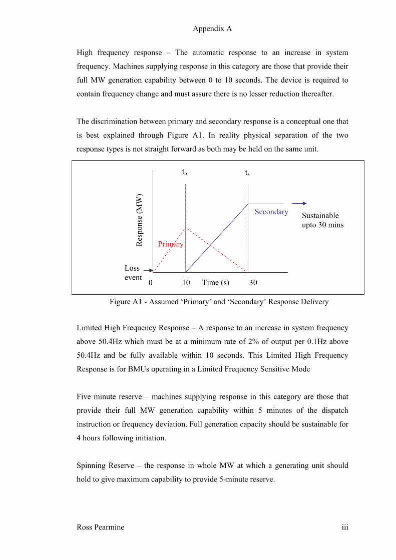
Appendix A
Ross Pearmine iii
High frequency response – The automatic response to an increase in system
frequency. Machines supplying response in this category are those that provide their
full MW generation capability between 0 to 10 seconds. The device is required to
contain frequency change and must assure there is no lesser reduction thereafter.
The discrimination between primary and secondary response is a conceptual one that
is best explained through Figure A1. In reality physical separation of the two
response types is not straight forward as both may be held on the same unit.
Limited High Frequency Response – A response to an increase in system frequency
above 50.4Hz which must be at a minimum rate of 2% of output per 0.1Hz above
50.4Hz and be fully available within 10 seconds. This Limited High Frequency
Response is for BMUs operating in a Limited Frequency Sensitive Mode
Five minute reserve – machines supplying response in this category are those that
provide their full MW generation capability within 5 minutes of the dispatch
instruction or frequency deviation. Full generation capacity should be sustainable for
4 hours following initiation.
Spinning Reserve – the response in whole MW at which a generating unit should
hold to give maximum capability to provide 5-minute reserve.
tp ts
Res
po
nse
(M
W)
Secondary
Primary
Figure A1 - Assumed ‘Primary’ and ‘Secondary’ Response Delivery
Loss
eventTime (s) 100 30
Sustainable
upto 30 mins

Appendix A
Ross Pearmine iv
Operating Reserve – additional output available from generating plant which must
be realizable in real-time operation to respond in order to contain and correct any
system frequency deviation in the event of a generation loss.
Generator response
The response of the generators falls into one of three categories [3] autonomous
generation response for fast (< seconds) fluctuations, regulation by the AGC
(seconds-minutes) or manual load following (minutes-hours).
The differences in the three functions affect the type of generator unit required to
respond to the load changes. Generators providing a regulating service must respond
quickly to frequent, small load changes. However, the load following generators will
respond to large, but slow changing loads.
Response contracts between National Grid and Balancing Mechanism Units (BMUs)
are confirmed by response profiles that provide accurate response details for each
BMU. These profiles are supplied for a range of frequency deviations from 0.1 to
0.8 Hz.
Balancing Mechanism Units [4] may be instructed to operate in either a Limited
Frequency Sensitive Mode or a Frequency Sensitive Mode (ie. to provide Primary
and High Frequency Response or Primary, Secondary and High Frequency
Res
po
nse
(M
W)
Load (MW)
deload 0 =
Availability
deload
deload
deload
deloaddeload Primary (-0.5Hz)
Primary (-0.8Hz)
Primary (dynamic)
Figure A2 - Sample response curve

Appendix A
Ross Pearmine v
Response). A BMU operating in the Limited Frequency Sensitive Mode will be
considered as frequency insensitive unless the system frequency exceeds 50.4Hz
when the BMU will be required to provide Limited High Frequency Response.
A BMU may be instructed to provide combinations of Primary, Secondary and High
Frequency Response with the combinations permissible, and the value of responses
realisable, being defined within the relevant Ancillary Services Agreement. Such an
instruction results in the BMU operating in a Frequency Sensitive Mode.
Calculation of Reserves for frequency response
Primary
Previous methods for calculating reserve in national grid [5], use a system network
model where all lines are lumped as a single transmission line. All loads were
connected to one end of the line and all generators are connected to other end of the
line. All MW demand lumped as one load and reactive MVAr demand was set to
zero. Generators were grouped into different types, i.e. nuclear, coal, CCGT etc.
Each generator type having its own governor/AVR models and the starting
frequency set to 50Hz.
Prim ary Response of G enerators
0
10
20
30
40
50
60
70
0 0.1 0.2 0.3 0.4 0.5 0.6 0.7 0.8 0.9
D eviation B elow 50 H z
Resp
on
se P
rovid
ed
Rt
Rx
Rt-1
ft-1
fx
ft
Figure A3 – Primary Response of generators
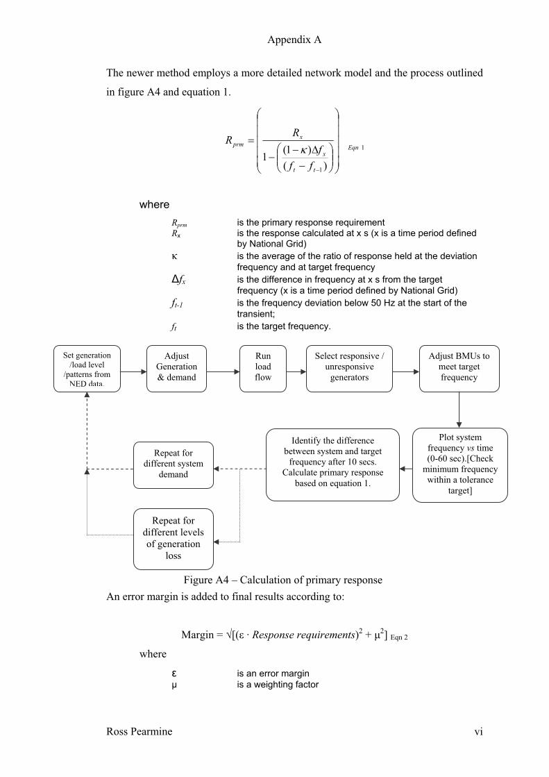
Appendix A
Ross Pearmine vi
The newer method employs a more detailed network model and the process outlined
in figure A4 and equation 1.
1
1)(
)1(1
Eqn
tt
x
xprm
ff
f
RR
where
Rprm is the primary response requirement Rx is the response calculated at x s (x is a time period defined
by National Grid)
is the average of the ratio of response held at the deviation
frequency and at target frequency
fx is the difference in frequency at x s from the target
frequency (x is a time period defined by National Grid)
ft-1 is the frequency deviation below 50 Hz at the start of the
transient;
ft is the target frequency.
An error margin is added to final results according to:
Margin = [( · Response requirements)2 +
2] Eqn 2
where
is an error margin
is a weighting factor
Set generation
/load level
/patterns from
NED data.
Run
load
flow
Select responsive /
unresponsive
generators
Identify the difference
between system and target
frequency after 10 secs.
Calculate primary response
based on equation 1.
Plot system
frequency vs time
(0-60 sec).[Check
minimum frequency
within a tolerance
target]
Adjust BMUs to
meet target
frequency
Repeat for
different levels
of generation
loss
Repeat for
different system
demand
Adjust
Generation
& demand
Figure A4 – Calculation of primary response

Appendix A
Ross Pearmine vii
Secondary
NGT currently calculate secondary response using the formula:
3secmax,&cotsec ))1()(1(
EqnWEs fDfdRiskR
where
Rsec is the secondary response requirement
is an error margin
Risk is the level of risk for which response is being calculated
is the sensitivity of demand to changes in frequency
fdscot is the Scottish demand as a fraction of NGC demand DE&W is the NGC demand
fmax,sec is the maximum frequency deviation allowed on secondary
response time scales
Other Approaches to reserve calculation
A paper from Taiwan University [6] looking at the Taiwanese Grid (60Hz) proposes
that reserve be divided into four categories; frequency regulating, instantaneous,
extended and stand-by reserves. For comparison frequency regulating and
instantaneous reserves are equivalent to national grids primary and secondary
reserve respectively.
RSRR = Max[SR, PGmax] Eqn 4
SR = Psystem × ( PL/ f) × (60-f1) Eqn 5
FRR = Psystem × ( PL/ f) × (60-f2) Eqn 6
IR = RSRR-FRR Eqn 7
Where
RSRR is the reasonable spinning reserve SR is the spinning reserve Psystem is the system load
PL/ f is the load-frequency sensitivity factor
IR is the instantaneous reserve FRR is the i frequency regulating reserve f1 is the frequency of load shedding f2 is the margin to f1PGmax is the output from the largest generator
In these equations FRR and IR are equivalent to National Grid Primary and
secondary responses respectively.

Appendix A
Ross Pearmine viii
Presented in the paper and others [7], [8] is a method for calculation of the value of
, the sensitivity of demand to changes in frequency, equation 8. National Grid
currently uses a value of 0.02, which has been developed through operating practice
and confidence in the system security. The presented papers employ a statistical
approach to calculate the mean ( ) and standard deviation ( ) of the demand
sensitivity to frequency based on forced generator outages during a five year period.
The factor for each seasonal day is calculated from system data for three separate
load periods; hours 0-6, 7-14 and 15-23. Demand sensitivity to frequency is then
calculated depending on the rate of change of the system load and the use of pumped
storage (Table 1), typical values range from 0.0857 – 0.1212.
8Eqnf
P
f
P[pu.Hz
-1]
Pumped storage No pumped
storage
0dt
dPsystem( – ) ( )
0dt
dPsystem( – ) ( + )
The sensitivity of a system load to frequency can also be expressed by the load
damping factor [9], which represents the change in the power for a given change in
the frequency in an interconnected system. Typical values of 1% to 2% are common;
a value equal to 2 implies that a 1% change in frequency would cause a 2% change
in load. The smaller the changes in frequency for a given load change, the stiffer the
system. The per unit area transfer function using the total load as power base and 50
Hz as frequency base, can now be represented as follow:
9
1
)()()(
)(
EqntieLG sMDsPsPsP
sF
where
M is the combined inertia constant of the local machine and
the effective rotating inertia of all the other machines connected via the power system
D is the load damping factor
Table 1 - Criteria for calculating demand sensitivity to frequency

Appendix A
Ross Pearmine ix
The inertia constant of the power system can be estimated using the measured transients of
the frequency. Inoue et al [10] have used frequency transient responses from loss events and
load rejection tests to provide an approximation of the transient in estimating the inertia
constant. At the onset of an event the change in frequency ( f) is zero and substituted in
equation 10 system inertia becomes:
10
)/(
Eqn
o PfKdt
ffdM
where
M is the inertia constant of system
P is the amount of generation loss
K is the power/frequency characteristic [pu.Hz-1
]
f is the change in frequency
fo is the rated system frequency
The inertia constant for the Japanese grid system calculated from 10 events is around 14 to
18 seconds. It provides a set of estimated values corresponding to the Japanese Grid for K
(- P/ f) where f includes response, ranging from approximately 1.53 to 0.77 at a
transiently settled state 20 seconds after the event. It also suggests that a positive
correlation exists between the inertia constant and load damping, which influences the value
of system inertia for a given load.
A paper on the Irish electricity grid[11] uses locked governor tests to establish estimates of
inertia and load sensitivity to frequency. It approximates the LFSF to in order of 2-2.5% per
Hz and gives a system inertia of 5000 MJ or 1.6-1.8 MWs/MVA. The paper also
successfully simulates grid responses by use of low order generator models.
Mansoor [12], suggests without speed control governors and tie lines, the inertia and the
damping constants can determine the system response to a load change, and the steady state
frequency deviation can be calculated as
15Eqn
Lss
D
Pf
The steady state frequency deviation following a load change for a power system
with generator units operating in speed droop mode is given by equation 11.

Appendix A
Ross Pearmine x
11
1
11 Eqn
L
n
Lss
P
DRR
Pf
where
D is the frequency characteristic of load damping
R1…n is the speed droop for generators 1 to n
PL is the system load change
fss is the steady state frequency deviation
is the power system frequency response (stiffness) [MW.Hz-1
]
The physical significance of can be stated as follows; if a power system was
subject to a step load change, it would experience a static frequency drop inversely
proportional to its stiffness. The smaller the changes in frequency for a given load
change the stiffer the system. The steady-state relationship between load change,
frequency change and the increase in power output provided by the governor action
is shown in figure A6. The power output increase of each individual unit under
governor control is given by:
12Eqnunit
ssT
R
fP
A linear approximation [13] of the frequency response characteristic of the total
system can be expressed as.
13Eqnt
L
L
L
f
fK
P
P
14.
1
EqntTt
T
L
T
f
f
f
fK
P
P
where
KL is the frequency sensitivity of the power demand
KT is the reciprocal of droop for the total system generation
PL is the system load change
PT is the system generation change
T is the system droop
KL relates to the total system demand and tests conducted on actual systems indicate
the generation response characteristic is more dependent on frequency than the

Appendix A
Ross Pearmine xi
demand response characteristic. KL has typical values between 0.5 and 3 while KT is
approximately 20 ( T = 0.05). In the above equations KT and KL have the opposite
sign meaning an increase in frequency causes a drop in generation and an increase in
electrical load. A change in power demand can be expressed as.
15).(
Eqnt
L
t
LLTLTdemandf
fP
f
fPKKPPP
The coefficient = KT + KL is refered to as the stiffness.
Brief Introduction to Generators
The synchronous a.c. generator consists of two main components a stationary
element called a stator and a rotating member known as the rotor. These components
are separated by an air-gap and both carry copper windings. A rotating field machine
common in larger generators carries a d.c. field winding on its rotor, connection to
which is made via slip-rings and brushes.
Under steady state conditions the machine will operate at a synchronous speed but
an increase in the output power is only facilitated by an increase in input power to
the prime mover. This action will cause the rotor to accelerate above synchronous
speed until the new power balance is meet, at which point the machine will return to
its synchronous condition. If two or more generators are connected on the same
electrical system grid they will operate as if they are on the same shaft. The real
power generated depends on the prime mover torque, which is controlled in a
hydraulic turbine by the guide vane position.
It is often necessary to respond to changes in load as explained. This is achieved
through controlled changes to the operating conditions of a generator and for this
two basic control elements are required the Governor and AVR (Automatic Voltage
Regulator). The AVR feeds back the generator terminal voltage and compares this
with a reference signal. The resulting error signal is amplified and fed into the
controller for the field voltage. The purpose of the governor is to control the amount
of power transferred to the power system by maintaining a balance between the
input shaft power and the exported electrical power.
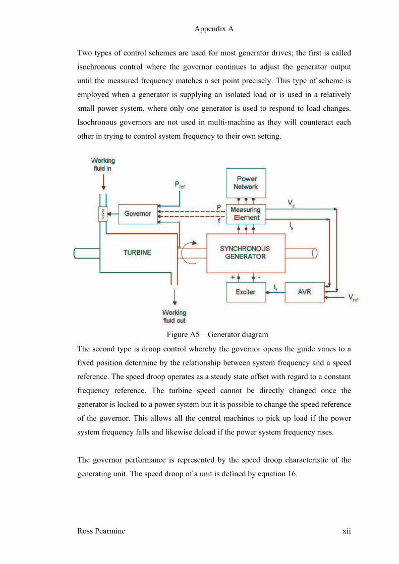
Appendix A
Ross Pearmine xii
Figure A5 – Generator diagram
Two types of control schemes are used for most generator drives; the first is called
isochronous control where the governor continues to adjust the generator output
until the measured frequency matches a set point precisely. This type of scheme is
employed when a generator is supplying an isolated load or is used in a relatively
small power system, where only one generator is used to respond to load changes.
Isochronous governors are not used in multi-machine as they will counteract each
other in trying to control system frequency to their own setting.
The second type is droop control whereby the governor opens the guide vanes to a
fixed position determine by the relationship between system frequency and a speed
reference. The speed droop operates as a steady state offset with regard to a constant
frequency reference. The turbine speed cannot be directly changed once the
generator is locked to a power system but it is possible to change the speed reference
of the governor. This allows all the control machines to pick up load if the power
system frequency falls and likewise deload if the power system frequency rises.
The governor performance is represented by the speed droop characteristic of the
generating unit. The speed droop of a unit is defined by equation 16.

Appendix A
Ross Pearmine xiii
16%100
)(%
Eqno
flnl
f
ff
P
wfR
where
R% is the droop
ffl is the steady state frequency full load
fo is the rated frequency
fnl is the steady state frequency no load
is the machine speed
A typical droop characteristic for the UK is 4% as specified in the Grid Code
CC6.3.7, which means that a frequency deviation of 4% (2 Hz) causes a 100%
change in the generator output. The load frequency control characteristic of the
power system depends on the collective effects of all the droops of the speed
governors and on the frequency characteristics of the load damping.
Basic models for speed governing systems and turbines for power system studies are put
forward by a number of IEEE working groups. These include models for steam and hydro
turbines [14], hydraulic turbines [15] [16], and also fossil fired plants [17]. The papers
define various function block diagrams for turbine controls and when possible provides
typical parameters for such models. Adibi et al provide models of frequency response and
reserve for various generator types.
New load
Base load fnl
ffl
fss
f
PT
PL
Generator power output
Syst
em f
requen
cy
100%0
Figure A6 – Generator Characteristics (with speed droop)

Appendix A
Ross Pearmine xiv
Summary
In this review an introduction is made into the methods used by National Grid to
calculate primary and secondary response. Also included in the document are
various methods employed internationally to define a power load-frequency
characteristic, and examples of calculated values for those systems.

Appendix A
Ross Pearmine xv
References
[1] Understanding automatic generator control
Jaleeli, N.; Ewart, D.N.; Fink, L.H.;
Power Systems, IEEE Transactions on, Volume: 7 Issue: 3 , Aug. 1992
Page(s): 1106 –1113
[2] Energy storage and small generation for Frequency Control and Voltage Regulation
NGC/Rolls-Royce T&D development Group 1
Doc R-R T&D: 99105/892.05/001 NGC: TR(T) 315, Oct. 1998
[3] Defining intra- and interhour load swings
Hirst, E.; Kirby, B.;
Power Systems, IEEE Transactions on, Volume: 13 Issue: 4 , Nov. 1998
Page(s): 1379 –1385
[4] Economic dispatch advice for the NETA balancing mechanism
Dyer, J.R; Williams, T.G.;Dunnett, R.M.;
Power System Management Control, Conference Publication No. 488, Apr. 2002
Page(s): 1 – 6
[5] Calculation of response requirements
Williams, T.G;
Internal Report
April. 2003
[6] Online methodology to determine reasonable spinning reserve requirement for isolated
power systems
Wu, C.C.; Chen W.;
Generation, Transmission and Distribution, IEEE Proceedings in, Volume: 150 Issue: 4, July.
2003
Page(s): 455 – 461
[7] Frequency-based method for fast-response reserve in isolated power systems
Kelly, M.; Cooke, A.; Hope, J.;McNamara, F.;Witmarsh-Everiss, M.J.;Canning, T.O.M.;
CIGRE session 38-307, Aug. 1994
[8] Modelling of post generation loss frequency behaviour in power systems
Wu, C.C.; Chen W.;
Paper under consideration
[9] Estimation of Load-frequency sensitivity factor and reasonable spinning reserve in the
taiwan power system
Wu, C.C.; Chen W.;
Paper under consideration
[10] Behaviour and Operation of Pumped Storage Hydro Plants

Appendix A
Ross Pearmine xvi
Mansoor, S.;
PhD Thesis, University of Wales,
[11] Estimation of power system inertia constant and capacity of spinning reserve support
generators using measured frequency transients
Inoue, T.;Ikeguchi Y.;Yoshida, K.;
Power Systems, IEEE Transactions on , Volume: 12 Issue: 1, Feb. 1997
Page(s): 136 – 143
[12] Power system Dynamics and stability
Machowski, J; Bialek, J.W.; Bumby J.R.;
John Wiley & sons, 1997
[13] Dynamic models for steam and hydro turbines in power system studies
Power Apparatus & Systems, IEEE Transactions in , Volume: 92 Issue: 3, Nov. 1992
Page(s): 1904 – 1915
[14] Hydraulic turbine and turbine control models for system dynamic studies
Power Systems, IEEE Transactions on, Volume: 7 Issue: 1, Feb. 1992
Page(s): 167 –179
[15] Second Order Hydraulic turbine models for multimachine stability studies
Vournes, C.D.;
Energy Conversion, IEEE Transactions on , Volume: 5 Issue: 2 , June 1990
Page(s): 239 –244
[16] Dynamic models for fossil fueled steam units in power system studies
Power Systems, IEEE Transactions on, Volume: 6 Issue: 2, May 1991
Page(s): 753 –761
[17] Frequency response of prime movers during restoration
Adibi, M.M.; Borkoski J.N.; Kafka, R.J.; Volkmann, T.L.;
Power Systems, IEEE Transactions on, Volume: 14 Issue: 2, May 1990
Page(s): 751 –756

Reducing the environmental impact of frequency control on the UK power system against a
background of increasing renewable generation.
Ross Pearmine 1
Six Monthly Progress Report: Third Report
Section Title Page
1.0 Previous Work 2
1.1 Determining methods to calculate Load Sensitivity to
Frequency 2
1.2 Assess the statistical generator mix of response holding 4
1.3 Review of generator models 5
1.4 Other Objectives 7
2.0 Reviewing the scope of work 7
3.0 Review of objectives 8
4.0 Next 6 months 9
5.0 Summary 9
Appendix A i

Reducing the environmental impact of frequency control on the UK power system against a
background of increasing renewable generation.
Ross Pearmine 2
1.0 Previous Work
The following sections highlight progress made on objectives set out in the previous
six monthly reports (report two).
1.1 Determining methods to calculate Load Sensitivity to Frequency
Review of literature (Appendix A) shows that the value of load sensitivity used by
National Grid is in line with that of other systems. After analysis of existing
historical data it was found that the sampling period records is not small enough to
directly measure the dynamic changes of the load.
Using details of previous generation incidents a plot of minimum frequency against
generation disturbance allowed the network characteristic (kT) to be plotted,
Figure 1.0. Using Eqn 1 it should be possible to calculate the load response (kL) if
the generation characteristic (kG) is also known. The generation characteristic can be
calculated from knowledge of the total generation, the output of the responsive
generators and their droop setting. Figure 1.1 shows the generation characteristic
calculated for one of the generation incidents given in Figure 1.0.
kT = (kG + kL) Eqn 1
Figure 1.0 Network characteristic for generation losses between 1994 and 2004
Change in Frequency - %
0%
1%
2%
3%
4%
5%
6%
7%
8%
0.0% 0.2% 0.4% 0.6% 0.8% 1.0% 1.2% 1.4%
Average
droop
4.76 %
2.86%
8.89%
Dis
turb
an
ce - %

Reducing the environmental impact of frequency control on the UK power system against a
background of increasing renewable generation.
Ross Pearmine 3
For the event chosen at the point of generation loss the generation characteristic was
2.93%, and the network characteristic was 4.12%. This gives a Load sensitivity of
1.19%. Calculating the average load sensitivity to frequency for a total of 13 events
gives a value of 1.94%, but with a standard deviation of 1.88. This is a very wide
range of values.
On 5th
March 2004 the new Integrated Energy Management System (IEMS) went
live, replacing the older EMS. The IEMS provides essential facilities to enable the
electricity national control centre to manage and control the transmission grid
system and for the network operations centre to provide safe access to the system for
construction and maintenance. The IEMS interacts with other NGT computer
systems as well as having it own database and display facility.
An IEMS change request has been made to allow the logging of load, frequency and
generator details at intervals of 3 seconds during a generator loss event. This should
allow numerical verification of the load sensitivity to frequency. This is obviously
relies on a generator loss taking place and so cannot be given a firm timescale.
Typically the grid is affected by approximately six events a year, so it is likely that
the next event may occur within the next two months.
Figure 1.1 – Generation characteristic for UK grid July 2003
48
48.5
49
49.5
50
50.5
51
51.5
52
25000 30000 35000 40000 45000
Cum ulativ e Ge ne rator Output - MW
Ne
two
rk F
req
ue
ncy
- H
z
Normal system
operating point

Reducing the environmental impact of frequency control on the UK power system against a
background of increasing renewable generation.
Ross Pearmine 4
DTI energy industry statistics from 2002 illustrate how electric demand is split
between the various market sectors. Using the DTI data with that from the literature
review in Appendix A, we can get another source of what response to expect from
the cumulative UK loads.
Table 1.2 shows the average load-frequency characteristic for the entire network
from 2002 to be 1.78-1.94 %, which again is similar to those given in Appendix A.
Twh % of total
TWh
Load Frequency sensitivity
(for load types)
Domestic 114.5 29 0.7 - 1.0
Industry 111.7 28 2.6
Services 98.0 25 1.2 - 1.7
Energy Industry 61.9 16 2.9
Transport 8.5 2 1.2 -1.7
Total 1.78 - 1.94
Table 1.2 - Load-frequency characteristics of industry sectors
1.2 Assess the statistical generator mix of response holding
Figure 1.3 – Mix of plant used for Response (July 2001 to December 2003)
0%
20%
40%
60%
80%
100%
Ju
ly 0
1
Au
gu
st 0
1
Se
pte
mb
er
01
Octo
be
r 0
1
No
ve
mb
er
01
De
ce
mb
er
01
Ja
nu
ary
02
Fe
bru
ary
02
Marc
h 0
2
Ap
ril 0
2
Ma
y 0
2
Ju
ne
02
Ju
ly 0
2
Au
gu
st 0
2
Se
pte
mb
er
02
Octo
be
r 0
2
No
ve
mb
er
02
De
ce
mb
er
02
Ja
nu
ary
03
Fe
bru
ary
03
Marc
h 0
3
Ap
ril 0
3
Ma
y 0
3
Ju
ne
03
Ju
ly 0
3
Au
gu
st 0
3
Se
pte
mb
er
03
Octo
be
r 0
3
No
ve
mb
er
03
De
ce
mb
er
03
COAL CCGT OIL OCGT HYDRO 1%droop HYDRO 4%droop

Reducing the environmental impact of frequency control on the UK power system against a
background of increasing renewable generation.
Ross Pearmine 5
Work has begun on this aspect of the project during periods when other work has
been suspended pending input from other sources. A plot of the response
instructions to balancing plant (Figure 1.3) shows no real noticeable change in
trends. It was expected that CCGT plant would gradually be picking up more
response. However, a more detailed breakdown showing MW response of the
generator types is yet to be completed and this may show otherwise.
1.3 Review of generator models
Currently generators are modelled for some network stability studies in a software
package called Eurostag. Each of the generators has a specific governor and voltage
regulator model which together with alternator characteristics define its behaviour
during transients. During previous network studies it was believed that the
responsive generators provided more power than was to be expected. Investigations
comparing individual generators on a simple model with test data showed that the
generator did seem to be providing more response than was expected from the test
data, Figure 1.4 and 1.5.
Figure 1.4 – Simulation of X generator against response tests
0 20 40 60 80 100 120 140
Time - seconds
Ou
tpu
t -
MW
-0.6
-0.5
-0.4
-0.3
-0.2
-0.1
0
0.1F
req
ue
ncy
- H
z
Test data Simulation Test Finj Simulation
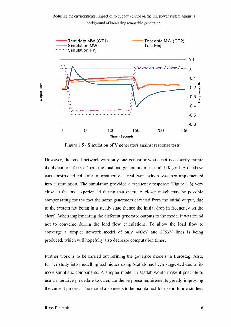
Reducing the environmental impact of frequency control on the UK power system against a
background of increasing renewable generation.
Ross Pearmine 6
However, the small network with only one generator would not necessarily mimic
the dynamic effects of both the load and generators of the full UK grid. A database
was constructed collating information of a real event which was then implemented
into a simulation. The simulation provided a frequency response (Figure 1.6) very
close to the one experienced during that event. A closer match may be possible
compensating for the fact the some generators deviated from the initial output, due
to the system not being in a steady state (hence the initial drop in frequency on the
chart). When implementing the different generator outputs to the model it was found
not to converge during the load flow calculations. To allow the load flow to
converge a simpler network model of only 400kV and 275kV lines is being
produced, which will hopefully also decrease computation times.
Further work is to be carried out refining the governor models in Eurostag. Also,
further study into modelling techniques using Matlab has been suggested due to its
more simplistic components. A simpler model in Matlab would make it possible to
use an iterative procedure to calculate the response requirements greatly improving
the current process. The model also needs to be maintained for use in future studies.
Figure 1.5 - Simulation of Y generators against response tests
0 50 100 150 200 250
Time - Seconds
Ou
tpu
t -
MW
-0.6
-0.5
-0.4
-0.3
-0.2
-0.1
0
0.1
Fre
qu
en
cy
- H
z
Test data MW (GT1) Test data MW (GT2)Simulation MW Test FinjSimulation Finj

Reducing the environmental impact of frequency control on the UK power system against a
background of increasing renewable generation.
Ross Pearmine 7
The benefit of a simple model in this case would be that no specialised technical
knowledge would be needed for the upkeep of the model.
1.4 Other Objectives
With the exception of assessing the impact of the location of loss/response holding
on response requirement no further modelling work can be carried out with the
Eurostag software until the generator models are verified. This means that assessing
the impact of the generator types and the impact of the starting frequency on
response requirement has been postponed until a later date. Time has not permitted
any simulations to be carried out to assess the impact of the location of loss and
response holding.
2.0 Reviewing the scope of work
As discussed in previous reports the chief aim of this project is to improve the
calculation of the response requirements and the understanding behind them. This
will allow the most economic (and usually also environmentally) beneficial response
holding which also enables National Grid to meet the statutory limits on frequency
deviation.
Figure 1.6 - Simulation of generator loss against record of actual event
49.3
49.4
49.5
49.6
49.7
49.8
49.9
50
0 10 20 30 40 50 60
Ti me - se c onds
Actual Network Frequency
Simulated Frequency

Reducing the environmental impact of frequency control on the UK power system against a
background of increasing renewable generation.
Ross Pearmine 8
The aim of the current work is to allow an accurate model of the system to be
created. This means improving models of demand and generator behaviour in
transients. Work has begun in understanding how load changes as a result of
changes in frequency following the sudden loss of generation. Review of the
Eurostag models aims to provide understanding of plant behaviour over response
delivery time scales in event of the loss. Once a complete picture of both these
stages is built validation of the system model against actual loss events can be
carried out.
With an model that accurately represents the system during transient behaviour it
will be possible to assess the margin in response requirements needed to allow for
modelling errors, failure of plant to deliver response and variation of initial
conditions, such as starting frequency. The model can then be applied to simulate
the effects of a changing generation mix. This is of particular interest with the new
government initiative to increase the share of renewable generation to 10 % by 2010
and then 15% expected by 2020.
3.0 Review of objectives
Manage the risk of failure to meet frequency obligations with cost and
environmental impact.
Modelling of demand-frequency relationship.
Validation of Eurostag models.
Statistical analysis of response delivery
Improving the response margin.
Establish error margins for Generator Mix / Specific plant.
Calculation of physical delivery of actual response on both primary and
secondary timescales.
Attend Modules
4.0 Next 6 months

Reducing the environmental impact of frequency control on the UK power system against a
background of increasing renewable generation.
Ross Pearmine 9
Develop a simple Eurostag network model to use in studies.
Assess the impact of the location of loss/response holding on
response requirement.
Assess the statistical generator mix of response holding.
Consider modelling techniques to use Matlab to mimic governor
responses.
Calculate load sensitivity to frequency from network data.
Produce paper to present at the EngD Conference
5.0 Summary
This report explains the current developments in calculating the load sensitivity to
frequency. It holds that the assumed National grid value of 2% seems to be accurate
but no quantifiable evidence can be produced to verify this accurately. Initial work
on the generator mix used for holding response seems to indicate that the types of
plant used have not dramatically changed since the July 2001. However, further
work must be carried out on this aspect.
Verification of the governor models used in Eurostag has shown that although
seemingly more responsive on an individual basis, if used collectively in a network
model results seem to corroborate with recorded data from real events. Further tests
are required on the full network model to confirm it is appropriate.
Highlighted in the document are the expected objectives for the research to improve
the generator response understanding in both the short and long term. Within the
next six months it is hoped that a functional network model will be produced to
allow further studies to be completed.

Appendix A
Ross Pearmine i
Appendix A – Literature Review
1. Introduction
An electrical supply system comprises of a collection of generating units and also
many loads, which are continuously varying over the course of the day in a largely
predicable manner. Changes in the consumer demands require an equal change in
generator outputs to maintain the system power balance. If a balance is not met
stored energy in the loads and/or generators are released, as this release is not
instantaneous it is seen as change in system frequency.
The network power-frequency characteristic affects the dynamic behaviour of the
power system and defines the ability of the system to compensate for a power
imbalance at the cost of a deviation in frequency. The power-frequency
characteristic is influenced by two elements; a demand (or load) component and a
generator component.
2. Generators
A system with many generator units operating under governor action will have a
very large generator characteristic and consequently a large power change will only
lead to a very small deviation in frequency. The generation characteristic is largely
dependant on the power available in the system, i.e. number of ‘responsive’
generators operating with their actual load away from their maximum power rating.
The generation characteristic of a system is non-linear because of these responsive
generating units. When the system power is in equilibrium the generator
characteristic can be approximated at the operating point by a linear characteristic
equation 1.

Appendix A
Ross Pearmine ii
tTt
T
L
T
f
f
f
fK
P
P.
1 (1)
where
KT is the frequency sensitivity of the total system generation
PL is the total system load
PT is the system generation change due to frequency
T is the system droop
f is the change in system frequency
ft is the rated system frequency
3. Loads
System loads are also frequency sensitive and a load-frequency characteristic is
required to relate the system demand to the system frequency, equation 2.
t
L
L
L
f
fK
P
P (2)
where
KL is the frequency sensitivity of the power demand
PL is the system load change due to frequency
4. Power-Frequency Characteristic
In the above equations KT and KL have the opposite sign meaning an increase in
frequency causes a drop in generation or increase in electrical load. This gives the
change in system power demand as:
t
L
t
LLTLTdistf
fP
f
fPKKPPP ).( (3)
where
is the stiffness (sometimes referred to as ~ power-
frequency characteristic)
Pdist is the disturbance power
5. Assessment of Power-Frequency Characteristic

Appendix A
Ross Pearmine iii
National Grid currently uses a value of 2 %MW/%Hz for its load-frequency
sensitivity, which has been developed through an understanding in operating
practice and confidence in the system security.
Papers from Taiwan University [1], [2] and [3] looking at the Taiwanese Grid (peak
load 25000MW @60Hz) use a method to calculate the value of the load-frequency
sensitivity factor, equation 4. The factor is calculated for each season, with each day
split into three separate load periods, Table 1.
0:00-7:59 hours 8:00-15:59 hours 16:00-23:59 hours
Spring 0.109109 0.088814 0.087569
Summer 0.097925 0.090716 0.087767
Autumn 0.092095 0.091635 0.085730
Winter 0.106481 0.094925 0.079947
f
P
f
PFactorySensitivitFrequencyLoad [pu.Hz
-1] (4)
where
f is the maximum frequency deviation
P is the generation loss
Table 1 – Mean values of Power-Frequency Factor, Taiwanese system
Figure 1 – Frequency incident on the Japanese grid
60.08
60.04
60.00
59.96
59.92
59.88
59.84
59.80
59.76
59.72
59.68
59.64
59.60
59.56
59.52
59.48
59.44
Sy
stem
Fre
quen
cy
(H
0 20 40 0 20 40 0 20 40 0 20 40 0 20 40 0
Time (Sec)
06/06/2002 12:20:00 Frequency Variation History Curve 300 Sec
Load shedding initiate
Appendix A
Ross Pearmine iv
After closer inspection of the methodology it is believed that the calculated factor
includes both load and generation characteristics, and relates to the power-frequency
characteristic. Figure 1 shows a frequency variation curve used in the paper
following the loss of an on-line generator (950MW). The magnitude of system load
demand was 21700 MW. The pre-fault frequency was 60.04 Hz and the minimum
frequency at the instant following the loss of the generator was 59.44 Hz, so the f
was taken as 0.6 Hz. These values were substituted in equation (4) to compute the
LFSF, which was 0.072965 in this case.
Equation (4) is only a measure of load-sensitivity to frequency if we assume that no
generation power is released before the peak deviation. As the frequency peak does
not occur until 20 seconds after the disturbance generators are likely to provide or
have started to provide response.
Inoue et al. [4] have used frequency transient responses from loss events and load rejection
tests to provide an estimation of the system inertia constant for the Japanese grid system
(14-18 secs). The paper also provides a set of estimated values corresponding to the
Japanese Grid (peak load 87400MW @60Hz) for power-frequency characteristic (- P/ f),
ranging from approximately 7.7 to 15.3 %MW/%Hz at a transiently settled state 20 seconds
after the event.
The Power System Study Committee: Japan [5], also carry out a number of experiments to
establish the power-frequency characteristic of Japanese grid. The tests establish a value of
8.5-14.6 %MW/%Hz.
A paper on the Irish electricity grid (peak demand of 4091MW) uses locked governor tests
to establish estimates of inertia and load sensitivity to frequency [6]. It approximates the
load-frequency characteristic in the order of 2-2.5 %MW per Hz and gives a system inertia
of 13-15 GJ equivalent to 5 MW/MVA. Kinetic energy stored in the Load was calculated as
5000 MJ or 1.6-1.8 MW/MVA.
A paper released on behalf of the UCPTE (230 GW @50Hz) [7] gives values for the
network power characteristic between 1988 and 1998 as 6.7 - 9.6 %MW/%Hz and Load
sensitivities in the order of 0.5 to 2.0 %MW/%Hz (see Figure 2).
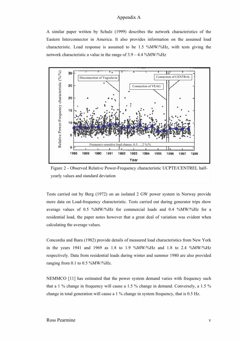
Appendix A
Ross Pearmine v
A similar paper written by Schulz (1999) describes the network characteristics of the
Eastern Interconnector in America. It also provides information on the assumed load
characteristic. Load response is assumed to be 1.5 %MW/%Hz, with tests giving the
network characteristic a value in the range of 3.9 – 4.4 %MW/%Hz
Tests carried out by Berg (1972) on an isolated 2 GW power system in Norway provide
more data on Load-frequency characteristic. Tests carried out during generator trips show
average values of 0.5 %MW/%Hz for commercial loads and 0.4 %MW/%Hz for a
residential load, the paper notes however that a great deal of variation was evident when
calculating the average values.
Concordia and Ihara (1982) provide details of measured load characteristics from New York
in the years 1941 and 1969 as 1.8 to 1.9 %MW/%Hz and 1.8 to 2.4 %MW/%Hz
respectively. Data from residential loads during winter and summer 1980 are also provided
ranging from 0.1 to 0.5 %MW/%Hz.
NEMMCO [11] has estimated that the power system demand varies with frequency such
that a 1 % change in frequency will cause a 1.5 % change in demand. Conversely, a 1.5 %
change in total generation will cause a 1 % change in system frequency, that is 0.5 Hz.
Figure 2 - Observed Relative Power-Frequency characteristic UCPTE/CENTREL half-
yearly values and standard deviation
Rel
ativ
e P
ow
er-F
requ
ency
char
acte
rist
ic (
%/%
)
Disconnection of Yugoslavia
Connection of VEAG
Connection of CENTRAL
Frequency-sensitive load change, 0.5…..2 %/%

Appendix A
Ross Pearmine vi
A report published by Eskom in 2000 [12] covers the frequency standards and levels of
control for various interconnected systems and the designation of the frequency standard in
the Southern African Power Pool. Table 2 gives the summarised results for the African pool,
the values are calculated from incidents of significant loss in generation. As the precise
methodology for calculations is not given this could mean the data is a measure of the
network characteristic rather than the load-frequency characteristic as specified in the report.
Incident Date Total Load Frequency
Characteristic
Load Frequency Characteristic
%MW/%Hz
(MW/Hz) Assuming the peak
load (30,000MW)
Assuming minimum
load (20,000MW)
132 19-Jul 1600 2.7 4
137 27-Jul 1510 2.5 3.8
139 28-Jul 1270 2.1 3.2
144 05-Aug 1140 1.9 2.9
145 05-Aug 950 1.6 2.4
146 05-Aug 1000 1. 7 2.5
Average 1250 2.1 3.1
Table 2 – Values of Network-characteristic for the Southern African Power Pool
Figures published by an IEEE task force on load representation [13] give constants for
frequency sensitivity for both active and reactive power. The findings are given in table 3.
Values for residential loads differ from those suggested by Concordia by at least 50%. This
discrepancy may be due to the change in load mix within the ten year period.
Load Power Factor Kpv Kqv Kpf Kqf
Residential
Elec Heating 0.87 to 0.99 0.9 to 1.7 2.4 to 2.7 0.7 to 1.0 -2.3 to -1.5
Non-Elec Heating 0.89 to 0.97 1.2 to 1.6 2.5 to 3.1 0.7 to 0.9 -2.3 to -1.3
Commercial
Elec Heating 0.85 to 0.9 0.5 to 0.6 2.5 1.2 to 1.5 -1.1 to -1.6
Non-Elec Heating 0.87 to 0.9 0.7 to 0.8 2.4 to 2.5 1.3 to 1.7 -1.9 to –0.9
Industrial 0.85 0.1 0.6 2.6 1.6
Aluminium 0.9 1.8 2.2 -0.3 0.6
Steel Mill 0.83 0.6 2.0 1.5 0.6
Power Aux. Plant 0.8 0.1 1.6 2.9 1.8
Agricultural Pumps 0.85 1.4 1.4 5.6 4.2
Table 3 – Typical load voltage parameters
Welfonder et al. (1989) provide results from load dependency tests carried out on parts of
the German grid system. Load monitoring equipment sited at Heidelberg (150MW demand)
and Berlin (80MW demand) provide a source of data for measuring the voltage and

Appendix A
Ross Pearmine vii
frequency dependency of the loads. In the respective sites the Load-frequency characteristic
is evaluated as 1.2 %MW/%Hz at Heidelberg and 0.8 %MW/%Hz at Berlin. The difference
at the sites is attributed to a higher constituent of motor load in the Heidelberg area.
6. Summary
KL
(%MW/%Hz)
KT
(%MW/%Hz)
NGT 2 (assumed) - -
Taiwan [1]-[3] - - 8.57 - 12.12
Japan [4] - - 8.5 - 14.6
Japan [5] - - 7.7 - 15.3
Ireland [6] 2 – 2.5 - -
UCPTE [7] 0.5 – 2 - 6.7 - 9.6
Norway [10] 0.4 - 0.5 - -
New York [9] 1.8 - 2.4 - -
America (Eastern Interconnection) [8]
1.5(assumed)
- 3.9 - 4.4
NEMMCO [11] 1.5 (estimate) - -
South Africa [12] (1250 MW/Hz) ~2.5
- -
Germany (part system)
[13]08 - 1.2 - -
Residential Loads [9] 0.1 - 0.5 - -
Residential Loads [14] 0.7 to 1.0 - -
Commercial Loads [14] 1.2 to 1.7 - -
Industrial Loads [14] 2.6 - -
Power Aux. Plant [14] 2.9 - -
Agricultural Pumps [14] 5.6 - -
Table 4 - Sensitivity Factors and Power-frequency characteristics
Results from various sources suggest that the typical power-frequency characteristic
of a system will range from 4 to 15 %MW/%Hz. Tests conducted on actual systems
indicate the generation response characteristic is far more dependent on frequency
than the load response characteristic. KL has typical values between 0.5 and 2.5
while literature [15] suggests KT is approximately 20, corresponding to a system
droop of 5%. Table 4 summarises the characteristic values given in this report.
Although no numerical background relating to the actual physical network has been
used in developing the NGT Load-frequency characteristic, comparisons with values
derived from other systems seem to place it within an acceptable band.

Appendix A
Ross Pearmine viii
The network-frequency characteristic is a parameter that can be control by NGT to
provide the most beneficial dynamic response to frequency. Although the Load-
frequency characteristic is predetermined by consumer behaviour, generator
scheduling solely determines the generation characteristic. Both the number of
generators and how the response is held on plant effects the overall generation
frequency dependency and hence the network-frequency characteristic.
It would be beneficial to provide a quantitative proof elucidating the NGT load-
frequency characteristic, which is used to provide the background for calculating the
secondary response requirement. With a loss of generation the reduction in demand
with frequency lowers the maximum risk on the network, meaning less response is
needed. If the value of the load-frequency characteristic is much greater than
anticipate excess response is being allocated to the system and can result in reduced
expenditure in that area, typically costing the company £43.5M1 per year.
1 Based on 2002/2003 financial year

Appendix A
Ross Pearmine ix
7. References
[1] Online methodology to determine reasonable spinning reserve requirement for isolated
power systems
Wu, C.C.; Chen W.;
Generation, Transmission and Distribution, IEEE Proceedings in, Volume: 150 Issue: 4, July.
2003
Page(s): 455 – 461
[2] Modelling of post generation loss frequency behaviour in power systems
Wu, C.C.; Chen W.;
Paper under considersation
[3] Estimation of Load-frequency sensitivity factor and reasonable spinning reserve in the
taiwan power system
Wu, C.C.; Chen W.;
Paper under considersation
[4] Estimation of power system inertia constant and capacity of spinning reserve support
generators using measured frequency transients
Inoue, T.;Ikeguchi Y.;Yoshida, K.;
Power Systems, IEEE Transactions on , Volume: 12 Issue: 1, Feb. 1997
Page(s): 136 – 143
[5] Field-test of power-frequency characteristics in 60Hz interconnected power system
Kelly, M.; Cooke, A.; Hope, J.;McNamara, F.;Witmarsh-Everiss, M.J.;Canning, T.O.M.;
JIEE of Japan, Volume: 97B Issue: 1, 1977
Page(s): 45 – 51 (in Japanese)
[6] Frequency-based method for fast-response reserve in isolated power systems
Kelly, M.; Cooke, A.; Hope, J.;McNamara, F.;Witmarsh-Everiss, M.J.;Canning, T.O.M.;
CIGRE session 38-307, Aug. 1994
[7] Characteristic numbers of primary control in the ucpte power system and future
requirement.
Weber, H.; Asal, H. P.; Grebe, E.;
ETG '97 summer meeting, July 21 - 22, Berlin, Germany
[8] Modeling of governing response in the eastern interconnection.
Schulz, R. P.;
1999 Winter Power Meeting, “ symposium on frequency control requirements, trends and
challenges in the new utility environment”
Page(s): 561 - 566

Appendix A
Ross Pearmine x
[9] Load representation in power system stability studies
Concordia, C.; Ihara, S.;
Power Apperatus and Systems, IEEE Transactions on , Volume: PAS-101 Issue: 4, Apr. 1982
Page(s): 136 – 143
[10] System and load behaviour following loss of generation
Berg, G.J.;
Procedings of IEE, Volume: 119 Issue: 10, Oct. 1972
Page(s): 1483 – 1486
[11] Discussion Paper: Generation and Load Measurement
National Electricity Market Management Company Limited
ACN. 072 010 327, Version No: 1.0, 15 January 2002
[12] Interim report on frequency relaxation project
Chown, G.; Coker, M.;
Eskom, August 2000
[13] Load representation for dynamic performance analysis
IEEE task force on Load representation for dynamic performance
Power Systems, IEEE Transactions on , Volume: 8 Issue: 2, May 1993
Page(s): 472 – 482
[14] Investigations of the frequency and voltage dependence of load part systems using a digital
self-acting measuring and identification system
Welfonder, E.; Weber, H.; Hall, B.;
Power Systems, IEEE Transactions on , Volume: 4 Issue: 1, Feb 1989
Page(s): 19 – 25
[15] Power systems dynamics and stability
Machowski, J.; Bialek, J. W.; Bumby, J. R.;
John Wiley & Sons, 1998
Page(s): 262 – 263

Reducing the environmental impact of frequency control on the UK
power system against a background of increasing renewable generation
24th
Monthly Progress Report
R.Pearmine
Brunel University
Y.H.Song Academic Supervisor
Brunel University
T.G.WilliamsIndustrial Supervisor
National Grid

24 Month Report R.Pearmine
i
Section Title Page
0 Executive Summary
0.0 Executive Summary 1
1 Introduction
1.0 Introduction 3
1.1 Document Structure 5
2 Environment
2.0 Impact of Frequency Response 6
2.1 Environmental Performance of Grid Connected
Generation 8
2.1.1 Coal fired power stations 9
2.1.2 Gas fired power stations 9
2.1.3 Biomass as a fuel 10
2.1.4 Nuclear Power 10
2.1.5 Hydroelectric and Tidal Power 11
2.1.6 Pumped Storage 11
2.1.7 Wind Turbines 11
2.1.8 Solar - Photovoltaic Power 11
2.2 Environmental Scope 12
2.3 Renewable Generation 13
3 System Frequency Response
3.1 Denmark, Sweden, Finland and Norway 15
3.2 Germany 18
3.3 New Zealand 19
3.4 Crete 20
3.5 Summary of operator experiences 21
4 Frequency simulations
4.0 The need for frequency simulations 22
24 Month Report R.Pearmine
ii
4.1 EUROSTAG a solution to model
frequency response 24
4.2 Modelling functions 25
4.3 The Dynamic Model and Simulation 27
4.4 The Network Model 29
4.5 Simulations using Eurostag 30
5 System Frequency Response
5.0 Frequency Response 31
5.1 Generator Droop 33
5.1.1 Generators 33
5.1.2 Impact of Droop on the Power System 34
5.1.3 Generator Droop Simulations 37
5.2 Disturbance Magnitude 38
5.2.1 Typical disturbance levels 38
5.2.2 Disturbance Simulations 39
5.3 Generator inertia 41
5.3.1 Effects of inertia 41
5.3.2 Inertia simulations 42
5.4 Load Frequency Sensitivity 44
5.4.1 Load Frequency Characteristic 44
5.4.2 Load Frequency simulations 44
5.5 Scheduling Generator Response 45
5.6 Generators for frequency response 48
5.6.1 Thermal Plant 48
5.6.1.1 Nuclear Stations 48
5.6.1.2 Coal and Oil-fired Stations 48
5.6.1.3 Biofuels 49
5.6.2 Steam Turbines 50
5.6.3 Gas Turbines 51
5.6.4 Hydroelectric Generation 53
5.6.5 Wind Power 55

24 Month Report R.Pearmine
iii
6 Work to Date
6.0 Modelling Objectives 57
6.1 Load Behaviour 58
6.2 Load Behaviour on the GB grid 59
6.3 Generator Behaviour on the GB grid 63
6.4 Future Work 68
6.5 Time Scales 71
7 Conclusion
7.0 Conclusion 72
8 References
8.0 References 74

24 Month Report R.Pearmine
iv
List of Figures
Figure 1 - Load duration curve showing breakdown of grid connected generation ......6
Figure 2 - Part-load efficiency of a CCGT generator ....................................................7
Figure 3 - Instructions issued to spinning plant for frequency response 2002-2004 .....7
Figure 4 - Generation mix by installed capacity[DTI (2000)]
.............................................8
Figure 5 - Gaseous Emissions from UK Electricity [Electricity Association (2003)]
....................9
Figure 6 - Growth of renewable generation [DTI (2004)]
..................................................13
Figure 7 - Nordic generation mix and interconnector capacities [Nordel (2003)]
...............16
Figure 8 - Governor transfer function..........................................................................28
Figure 9 - Various turbine transfer functions...............................................................29
Figure 10 - Block diagram of generator control system ..............................................33
Figure 11 - Generation characteristic from a July morning, 2003...............................35
Figure 12 - Speed-droop characteristics of steam and hydro turbines.........................36
Figure 13 - System droop for generation losses between 1994 and 2004 ...................36
Figure 14 - Effect of Generator droop on System frequency.......................................37
Figure 15 - Distribution of size of abnormal generation loss between 1987-2003......38
Figure 16 - Typical Grid Demand levels .....................................................................39
Figure 17 - Effect of disturbance magnitude on system frequency .............................40
Figure 18 - Effect of inertia on system frequency .......................................................42
Figure 19 - Effect of load sensitivity on system frequency .........................................44
Figure 20 - Example generator response profile curve................................................46
Figure 21 - Generator response to applied test frequency injection signal..................47
Figure 22 - Typical steam boiler arrangements used in power stations.......................49
Figure 23 - Non-reheat steam turbine ..........................................................................50
Figure 24 - Diagram of a simple gas turbine ...............................................................51
Figure 25 - Single shaft tandem plant configuration ...................................................52
Figure 26 - Multi-shaft plant configuration .................................................................52
Figure 27 - Hydroelectric turbine arrangement ...........................................................53
Figure 28 - Dinorwig Hydroelectric pumped storage facility......................................54
Figure 29 - North Hoyle offshore wind installation.....................................................55
Figure 30 – Wind turbine connection arrangements....................................................56
Figure 31 – Recorded Load sensitivity to frequency on the GB system .....................61

24 Month Report R.Pearmine
v
Figure 32 - Generator loss under unclear load conditions ...........................................62
Figure 33 - Generator loss under constant load conditions..........................................62
Figure 34 - Simulation of CCGT turbine at deload of 110 MW..................................63
Figure 35 – Simulation of coal fired steam turbine at deload of 95 MW ....................63
Figure 36.a – Simulation of 1260MW generation loss from 26/05/03 (frequency) ....64
Figure 36.b – Simulation of 1260MW generation loss from 26/05/03 (responsive
generation) ................................................................................................................... 64
Figure 36.c – Simulation of 1260MW generation loss from 26/05/03 (non-responsive
generation) ................................................................................................................... 64
Figure 37 – Simulation of 615MW Generator loss on 16/09/04 .................................67
Figure 38 – Network response to 615MW Generator loss on 16/09/04 ......................67
List of Tables
Table 1 - Contribution to frequency response in the Nordic pool ...............................17
Table 2 - Sensitivity Factors and Power-frequency characteristics .............................59
Table 3 - Gantt chart showing expected project deliverables over the final two years
of the project ........................................................................................................71

24 Month Report R.Pearmine
vi
Nomenculture
List of Symbols
ACE area control error [MW]
Aw Swept area of the blades [m2]
ffl frequency full load [Hz]
FHP HP power fraction [%]
fnl frequency no load [Hz]
f0 base frequency [Hz]
g acceleration due to gravity [m.s-2
]
H inertia constant [s]
hH head height [m]
I n Current [A]
J inertia [kg.m2]
K Gain [%]
KL load-frequency characteristic [%.Hz-1
]
kpf demand sensitivity [%.Hz-1
]
KT generator-frequency characteristic [%]
P power mismatch between load and generation [MW]
Pactual measured [MW]
PE electrical power [MW]
PG generator power [MW]
Pi individual generator outputs [MW]
PL system load [MW]
PLoss loss of a known generation [MW]
PM mechanical power [MW]
Pplanned planned interchange [MW]
PT system power [MW]
R Droop [%]
TW water time constant [s]
TRH time constant for re-heaters [s]

24 Month Report R.Pearmine
vii
TCH time constant relating to the steam chest and inlet piping
system [s]
U b Voltage [V]
uw Wind speed [m.s-1
]
W water flow rate [m3.s
-1]
Y Admittance [S]
Frequency response [MW.Hz-1
]
efficiency [%]
a air density [kg.m-3
]
G Generator speed droop characteristic [%]
Gi individual generator droops [%]
T system speed droop [%]
w water density [kg.m-3
]
angular rotation [Rad.s-1
]
M mechanical driving torque [N.m]
E electrical torque [N.m]

24 Month Report R.Pearmine
viii
List of abbreviations
NGT National Grid Transco
TSO Transmission system Operator
UK United Kingdom
GB Great Britain
NZ New Zealand
OHL Over head lines
HV High voltage
EMS Environmental Management Systems
SF6 Sulphur Hexafluoride
CO2 Carbon dioxide
NOx Nitrogen oxides
CCGT Combined cycle gas turbine
OCGT Open cycle gas turbine
SO2 Sulphur dioxide
PM10 Particulate matter 10 m
CO Carbon monoxide
CHP Combined heat and power
UCTE Union for the co-ordination of transmission of electricity
BMU Balancing Mechanism Unit

24 Month Report Executive Summary R.Pearmine
1
0 Executive Summary
The system frequency of a synchronous power system, such as the GB grid, varies
due to the imbalance between the energy supplied to the network and the electrical
energy consumed. When large generating blocks are lost the system undergoes a
frequency swing with a magnitude relative to the size of loss. Limits are imposed on
the magnitude of frequency deviation to prevent, in worst case, collapse of the system.
The aim of this research is to develop an increased knowledge to manage the risk of
frequency obligations during loss of large portions of power.
Operation of frequency responsive thermal plant results in lower efficiencies and thus
increased emissions. The current response requirements must be reviewed to ensure
excess response is not being held against the current generation mix. Future increased
levels of wind turbines may alter the operational characteristics of the system
(primarily system inertia). This is compounded by additional levels of response
required because of the unpredictability of wind resources. Environmental
implications result from added renewables that increase the response requirement and
hence emission levels.
It is the objective of this research to assess the optimum response that must be held to
minimise environmental emissions but ensure the operational safety of the system in
both the current, and future situations. This research will aid in limiting the
environmental impact of frequency response while aiding engineers to implement
reserve schemes that do not compromise system security. The project itself looks at
two main areas: Modelling Generator response, and Modelling Load response.
0.1 Methodology to be used
Through a series of grid simulations this project will develop an understanding of how
the UK transmission network responds to loss in generation. These simulations will
be carried out with a set of models, which will be validated against actual conditions,
as well as through comprehensive and critical assessment of available literature.

24 Month Report Executive Summary R.Pearmine
2
0.2 Contribution to knowledge
World-wide very limited studies have been conducted in the area of frequency
response. This is mainly due to the security provided by large interconnected
generation areas such as Europe and America. In such systems generator loss leads to
a very insignificant deviation in frequency and as such is not a critical issue. Island
systems such as the one operating in the UK are more sensitive to the imbalance
between generated and consumed power. Anticipated contributions to knowledge of
this project include:
Quantification of the UK load-frequency sensitivity.
Effect of generator location on frequency response.
Influence of wind turbines on the frequency response requirement.
Understanding the environmental impacts of response holding
0.3 Planned papers
The following papers will be written and will be submitted to journals within the next
two years:
Load frequency characteristic of the UK grid.
This paper aims to describe the effects of load behaviour on the UK system during
frequency disturbances. It will provide examples of generator loss on the system and
the drop in frequency as a result. It is hope to include details of generator responses
also.
This paper will be submitted to the IEEE Transactions in power systems.
Impacts of renewable generation on frequency response.
This paper aims to describe the effects of renewable generation on the UK system
especially during frequency disturbances. It will provide results of simulation studies
carried on a representative model of the UK transmission network. The paper will
highlight potential problems that may arise from the expected increase of renewable
sources in the generation mix. This will include the physical impacts due to plant
behaviour and the impact due to extra response margin required for their operation.
This paper will be submitted to the IEEE Transactions in power systems.
24 Month Report Executive Summary R.Pearmine
3
1 Introduction
1.0 Introduction
The system frequency of a synchronous AC power system varies with the imbalance
between the energy supplied to the network by generators and the electrical energy
consumed by its loads. We will later see that when large generating blocks are lost the
system undergoes a frequency drop relative to the size of loss. Limits are imposed on
the magnitude of frequency deviation to prevent disconnection of customers from the
system or damage to equipment.
The most critical reason for this research is to formulate a response requirement that
does not breach National Grid guidelines on security and quality of supply. These
requirements define the level of response required to contain specific power losses. If
these requirements are over estimated the system becomes very secure against losses
and frequency will not deviate considerably from the nominal. This security is
delivered at the expense of excess cost and environmental emissions. Conversely,
under estimation results in a network at high risk
By the year 2010 it is expected that a considerable increase in renewable generation
will occur in the energy sector. Targets suggest that 10 % of energy production will be
from renewable sources by the end of the decade. No credible studies have been
conducted to investigate what effect this change in generation mix will have on the
way the system reacts in terms of frequency response.

24 Month Report Environmental Impacts R.Pearmine
4
With an inevitable change in the future energy mix frequency response studies are
required to plan ahead for the introduction of these new generators. Conditional on the
effects of introducing a larger percentage of renewable generation operational
strategies or procedures may need review.
World-wide very limited literature has been published in the area of frequency
response. This is mainly due to the security that is provided by large interconnected
generation areas such as Europe. In such systems generator loss leads to a very
insignificant deviation in frequency and as such is not a critical issue. Island systems
such as the one operating in the UK are more sensitive to the imbalance between
generated and consumed power. There is also a vast difference between each HV
power transmission network in each country, and also the generation mix supporting
it.
With these points in mind this research looks to answer the question; what level of
frequency response is currently required to limit environmental impact but not cause
undue risk? What will this requirement be in the future?
24 Month Report Environmental Impacts R.Pearmine
5
1.1 Document Structure
The following paragraphs give an explanation of the content of this report:
In Chapter 2 we examine the environmental consequences of frequency response, this
includes a summary of the environmental performance of each type of generator. An
introduction to renewable generators is also given, with an explanation for the focus
on wind turbines in particular.
Chapter 3 highlights the approaches of other countries to frequency response and how
the UK differs from those schemes. It also includes the experiences that added
renewables has on the running of those systems.
Chapter 4 justifies the need for frequency simulations and the problems associated
with alternative techniques to quantify the response requirements. A chosen
simulation tool is introduced together with the dynamic components needed for such a
tool.
In Chapter 5 we study the main factors that influence frequency response. These
include; droop, inertia, load, type of generator and disturbance level. Included in this
chapter are preliminary simulations using the response tool to demonstrate the
sensitivity of each factor on the frequency response.
Chapter 6 looks at the research carried out to date to improve the accuracy of the
chosen simulation tool. This involves the quantification of the load response to
frequency, and validation of generator models. Future work to be carried out over the
next 2 years of the research is also considered.
Chapter 7 provides a brief summary of the report

24 Month Report Environmental Impacts R.Pearmine
6
2 Environment
2.0 Impact of Frequency Response
Market forces dictate which power stations are called upon to supply generation to the
electricity grid to meet consumer demand. This base load of plant is operated to meet
the majority of demand. As the system is dynamic NGT, as transmission system
operator (TSO) in Great Britain, must balance any short-term differences in
generation and demand through the balancing market. A level of backup generation is
also required to cover instantaneous loss of the largest generating unit operating at
any time. To facilitate this dynamic requirement NGT instructs part-loaded plant to
provide the headroom for frequency response, Figure 1. This part loaded generation
operates under governor control, and acts to control the grid frequency.
Figure 1 - Load duration curve showing breakdown of grid connected generation
0%
20%
40%
60%
80%
100%
0% 10% 20% 30% 40% 50% 60% 70% 80% 90% 100%
Percentage of Year
Pe
rce
nta
ge
of
Pe
ak
De
ma
nd
DemandMarginal Generation capacity
required for response CCGT
Interconnections
Nuclear
Coal

24 Month Report Environmental Impacts R.Pearmine
7
Part load generation or spinning reserve, raises environmental concerns because of
reduced plant efficiencies (Figure 2), and with the case of gas fired plant results in
increased NOx emissions. A percentage of frequency response is also provided
through demand side management, which is facilitated through the disconnection of
industrial load. Demand management usually offers minimal environmental impacts
but it is dependent on the industrial processes that have been interrupted. Frequency
response cannot be held solely by demand side measures as the response is only
provided at discrete frequency trigger points.
Figure 2 - Part-load efficiency of a CCGT generator
Spinning reserve can be held on any type of plant but in the GB system, the majority
is held on coal fired generators as can be seen from Figure 3. As the mix of generating
plant connected to the grid changes it is likely that the mix of plant used for response
holding will also mirror this change to a certain extent. The differing types of
generation also impact the level of loading that is required to provide the same
response, due to the transient behaviour of different generator types.
Figure 3 - Instructions issued to spinning plant for frequency response 2002-2004
0.3
0.4
0.5
0.6
0.7
0.8
0.9
1
1.1
0.55 0.65 0.75 0.85 0.95 1.05
Load (pu)
Eff
icie
ncy
()
2002
71%19%
1%
9%
COAL
CCGT
OCGT
OIL
HYDRO
2003
73% 19%
1%
7%
2004
71% 22%
0%
7%

24 Month Report Environmental Impacts R.Pearmine
8
2.1 Environmental Performance of Grid Connected Generation
The generation mix of the system is a continual evolution of different energy sources
and has changed over recent years, Figure 4. An increasing proportion of gas plant has
been introduced which has replaced oil, coal and nuclear plants. Projections suggest
this trend will continue over the next ten years with renewables also competing for an
increased share of capacity. A diverse mix of generation is important for the secure
operation of the grid but some generators provide energy at a much greater cost to the
environment.
Figure 4 - Generation mix by installed capacity[DTI (2000)]
An ever-increasing demand for electricity has lead to investment in a growing
capacity of grid connected generators. Despite this increasing consumption, emission
levels of CO2, SO2, NOx and PM10 by the industry have fallen in recent years, Figure
5.
The subsequent sections give a brief introduction to the environmental impact of grid
based generators during their operational life.
0%
10%
20%
30%
40%
50%
60%
70%
80%
90%
100%
1990 1999 2003 2010 2015
Pumped storage
GT
Import
Renewable
Nuclear
Mixed Fuel
CCGT
Oil
Coal

24 Month Report Environmental Impacts R.Pearmine
9
Figure 5 - Gaseous Emissions from UK Electricity [Electricity Association (2003)]
2.1.1 Coal fired power stations
Burning coal releases significant levels of SO2, NOx, CO2, PM, and mercury into the
air. Environmental concerns surrounding the use of coal to produce energy include
global warming, acid rain, regional and local health issues, and the impacts of coal
transport and ash disposal. The goal of newer coal combustion technologies has been
to reduce the environmental impacts. In addition to the air emissions, most coal plants
have significant community impacts due to the transport and handling of the coal, and
a requirement for large quantities of cooling water.
An increasing number of plants have been retrofitted with abatement technologies
such as flue gas desulphurisation to help reduce emissions.
2.1.2 Gas fired power stations
The burning of natural gas releases fewer air emissions than coal. Compared to
similarly sized coal plants, natural gas plants release 50 percent less CO2. The greatest
24 Month Report Environmental Impacts R.Pearmine
10
emissions are NOx emissions, which are more significant when plant becomes part
loaded. NOx emissions can be minimised by the use of various control technologies.
Open cycle gas turbine (OCGT) plant efficiency is typically low, approximately 37
percent, so are commonly used as peak load plants or for black start, when high
amounts of energy are required very quickly. OCGT emissions include NOx, CO, and
CO2.
A combined cycle gas turbine (CCGT) is more efficient than a OCGT equivalent
because the hot rejected heat gases of the turbine are not vented to the atmosphere, but
are used to raise steam for a second electric generator. By combining the gas and
steam cycles, the plant can convert approximately 60 percent of the fuel energy into
electrical energy. CCGT plants also produce less NOx and CO2 emissions than an
OCGT plant.
2.1.3 Biomass as a fuel
Emissions from biomass combustion are generally less than from coal or natural gas.
Like coal or natural gas combustion, biomass combustion produces CO2. Biomass can
also emit lower amounts of NOx, produce less ash than coal, and release significantly
less toxic material such as mercury. A closed methane digestion system that burns
biogas on a farm or landfill would reduce the amount of methane lost to the
atmosphere. However, it would release emissions similar to those of a natural gas-
fired turbine, but in smaller quantities. Environmental impacts vary with the type of
biomass fuel used, although most fuels will have impacts related to burning and
storage.
2.1.4 Nuclear Power
The main concern is safety involving the storage and management of highly
radioactive spent nuclear fuel. Air emissions are not an issue with nuclear plants.

24 Month Report Environmental Impacts R.Pearmine
11
2.1.5 Hydroelectric and Tidal Power
As Hydroelectric plants use falling water to turn a turbine that drives a generator to
produce electricity they produce no air emissions. Their main environmental impacts
are related to the flooding of the landscape upstream, changing flows within the
stream banks downstream, dividing the stream into separated pools, and damaging or
killing young fish. The barriers created by dams constrain fish and other species to
specific pools, impacting their ability to survive and reproduce. The turbines have the
potential to damage or kill young fish if they are not filtered on the upstream side of
the dam
2.1.6 Pumped Storage
Pumped storage is essentially a hydroelectric plant circulating its water supply, hence
it is a net user of electricity. In most cases a pumping mode is operated during the
night when demands are low, this is beneficial in helping to stabilise the demand
profile over the course of a day. Inefficiency in pumping water and also the
conversion back to electrical power are a concern with this plant. Ecological impacts
regarding the cyclic filling and draining of the reservoir must be considered.
2.1.7 Wind Turbines
Wind power has low environmental impacts (no air or water emissions), but concerns
have been raised over aesthetics, noise, and mortality to flying birds and bats.
2.1.8 Solar - Photovoltaic Power
Compared to traditional methods of electric generation, solar power has few
environmental concerns. The primary impacts for larger systems are related to land
use and aesthetics and may be resolved through appropriate siting.

24 Month Report Environmental Impacts R.Pearmine
12
2.2 Environmental Scope
Assessing the environmental impacts of each and every generation plant and also each
type of emission is far beyond the intended scope and life of this research. With CO2
emission levels being such a dominant issue in the Governments legislation to reduce
greenhouse gases it would be reasonable to focus research on the production of this
specific gaseous emission. The overall intention would be to assess the levels of CO2
production corresponding to frequency responsive generation.

24 Month Report Environmental Impacts R.Pearmine
13
2.3 Renewable Generation
Commitment laid down by UK government in the Kyoto agreement (1997) has meant
that an increase in renewable generation is necessary to reduce CO2 levels in the
energy sector. The Renewables Obligation Order (2002) calls for electricity suppliers
to procure a greater level of electricity from renewable sources. At the moment these
generators only account for 1.3 % of the total generation capacity. From Government
based targets it is anticipated that this figure will rise to 10 % by 2010, and a further
10 % by 2020.
The impact of this renewable generation on the operation of the grid network is
unclear. A critical assessment of the potential impacts these forms of generation will
have on the current operation of the grid is needed. Figure 6 shows the current trends
in renewables over the past six years and a projection for the year 2010. If the current
growth in wind farms is to continue they will account for a large percentage of the
renewable mix. A press release from the British Wind Energy Association suggested
that by 2010 eight percent of the national capacity would come from wind based
sources. This view is also held by the DTI who believe, "Wind power, both on- and
off-shore, is presently the only economic scaleable technology and will deliver the
majority of the required growth in renewable energy to meet the 2010 target…"
Figure 6 - Growth of renewable generation [DTI (2004)]
0
500
1,000
1,500
2,000
2,500
3,000
3,500
4,000
4,500
1997 1998 1999 2000 2001 2002 2003 2010
Insta
lled
cap
acit
y -
MW
Other combustionSmall scale hydroSewage sludgeOffshore WindOnshore WindWaste combustionLandfill gas
24 Month Report Environmental Impacts R.Pearmine
14
In 2003, over 1GW of offshore wind farms where given planning permission, and 328
MW of onshore installations. If these farms are commissioned the current penetration
of wind would be more than doubled. At this level of penetration, wind will provide
the majority share of grid connected renewables.
Wind turbines are unlike landfill gas or waste combustion, which operate in a similar
manner to CCGT/OCGT or coal machines. As wind turbines do not operate like other
grid connected generators several frequency control issues arise. The variability of
wind sources has a direct influence on the output power from turbines. Any short-term
changes in wind speed will lead to a demand generation imbalance, which also effects
the instantaneous frequency. The erratic nature of wind means it is hard to forecast,
and thus it is possible that extra spinning reserve will be required to maintain the level
of frequency deviations on the system.
There are also concerns that electric converters used in variable-speed wind turbines
will be seen as inertia-less generators by the grid. Fixed-speed turbines will provide
some benefit from their inertia, but this is provided that frequency and voltage remain
within their operating limits. If large quantities of variable-speed wind turbines
displace conventional generation, the total system inertia will decrease. The grid
inertia helps to control the rate at which frequency drops when there is a sudden loss
of generation. However, Ekanayake et al(2003) have shown that variable-speed
turbines could in principal be controlled to provide the equivalent inertia.
With expectation of such a high wind penetration it would be reasonable to
concentrate studies only on the effects brought about by additional wind turbines on
the system. This gives scope to investigate the variability of wind power and the
unknown risks it brings to frequency control in GB. The effect of generator inertia is
also a concern that should be addressed in relation to frequency control.
Many papers exist that concentrate on the voltage stability of wind farms, Akhmatov
et al.(2003) and Rodriguez et al.(2002) for example, but limited work exists on the
study of frequency stability.

24 Month Report Operator experiences in other countries R.Pearmine
15
3 Operator experiences in other countries
3.1 Denmark, Sweden, Finland and Norway
The Nordic countries are well known for their continued commitment to sustainable
working practices and keenness to minimise environmental impacts. Eltra system
operator in Jutland (West Denmark) in particular has one of the highest capacities for
wind at 2347 MW, almost 32 % of total generation, Eltra(2003a). Eltra operates as
part of the european UCTE system connected through Germany and operates DC
links with Norway and Sweden, Figure 7. The neighbouring power systems give Eltra
the total import capacity of 3060MW. This is nearly equal to the maximum
experienced on the system in 2003.
The balancing of Danish grid is relatively easy in periods of low wind. In high wind
situations, large amounts of excess electricity can cause transmission problems on the
system especially as it does not have any pumped storage to absorb excess generation.
This is compounded by the legal obligation to accept all prioritised electrical energy.
Experience has shown that within one to two hours wind speeds can vary in the Great
Belt by an amount equivalent to two power stations. The over-production is more
likely to occur at night in winter months where it can be aggravated by the output of
the many CHP plants. Until very recently, any over-production could always be
exported via interconnectors to neighbours.
The large amount of wind electricity produced in Jutland seriously hinders balancing
of the Danish electricity supply system. This has lead Jutland to become a net
importer of electricity despite its large generation capacity, UCTE(2003).

24 Month Report Operator experiences in other countries R.Pearmine
16
Sweden Norway Finland
Germany
Denmark
4155
1040
1350
630
550
Poland
Russian
Federation
Lithuania
Latvia
Estonia
Belarus600
600
Hydropower %
Nuclear Power %
Other thermal power %
Other renewable power %
600
1280
1560
50
100
600 600
Interconnection
1280
120
4855
1040 670
600
1350
550
50
Figure 7 - Nordic generation mix and interconnector capacities [Nordel (2003)]
As a member of the UCTE Jutland has an obligation to supply 35MW of primary
response. Internally it holds ±100 MW of automatic regulating reserve, which must be
held on a minimum of three spinning units, Eltra (2003b). Manual upward regulating
reserve totalling 420 MW is held as a requirement based on the loss of its largest unit
at Enstedvæket (620 MW), this allows recovery of any interconnected power supplied
through the UCTE. A further 200MW of downward regulating reserve is held to
secure against demand loss. This reserve may be held on units outside of Jutland and
supplied through it interconnectors.
The national power systems in the remaining Nordic countries operate as one

24 Month Report Operator experiences in other countries R.Pearmine
17
synchronous system, Elkraft(1996). They are fortunate in having large capacities of
hydroelectric power available for frequency response. A primary reserve of at least
600 MW is held on the combined system for controlling the frequency between
operational limits (50 ± 0.1 Hz). Contributions to frequency response by each area are
made based on the demands experienced in the previous year.
The area control error(ACE) is used to detect the manual frequency control measures
that are to be performed. The instantaneous ACE can be calculated from the
deviation( P) between measured(Pactual) and planned interchange(Pplanned) and the
frequency deviation( f) from 50 Hz, Equation 1. Lindahl(2002) gives the actual
frequency response( ) required from each area in 2002, Table 1.
ACE = P + . f = (Pactual - Pplanned ) + f
Equation 1
Country (Area) Frequency Response
[MW/Hz]
Denmark (Zealand) 270
Finland 1050
Norway 2220
Sweden 2460
Nordel 6000
Table 1 - Contribution to frequency response in the Nordic pool
An instantaneous disturbance reserve is activated in reaction to a simultaneous loss of
power plant where frequency deviation ranges from –0.1 to –0.5 Hz. The maximum
capacity of the loss is assumed to be no more than 1200 MW, it is also assumed that
the load will supply 200 MW of self-regulation. Under these conditions the frequency
shall not fall below 49.5 Hz.
Operating in this fashion means that the Nordic transmission system can share its
frequency response requirements between its member countries. This reduces the
number of plant required to hold response and as a consequence increases efficiencies
and reduces emissions.
24 Month Report Operator experiences in other countries R.Pearmine
18
3.2 Germany
Germany is composed of 4 TSOs, and has operational experience with the biggest
penetration of wind on any network with a capacity of 14345MW. 6250MW of
German’s wind turbines are in the E.ON Netz control area, E.ON(2004). This is
comparable to the level of wind generation that is to be expected in the UK by 2010.
Through operations the TSO has noted that a reliable weather forecast is foremost to
maintaining a stable grid frequency.
E.ON's Wind Report highlights the use of reserve capacities of up to 60% of the
installed wind power capacity for wind balancing. One occasion when generation
dropped 3640MW within six hours, with an average value of 10MW per minute raises
particular concerns on wind variability. The report imparts a concern that wind farm
construction should be tempered by a realistic recognition of the high costs and
serious engineering difficulties experienced during operation.
Germany is connected to the UCTE system via neighbouring states. As such it is
required to contribute to the 3000MW primary control that is held on the system. The
UCTE operates in a similar manner to the Nordic system, where the proportion of
response is calculated based on total demand. Power transfers are required in the
event that system frequency drops from nominal 50 Hz and should be limited to ±0.2
Hz.

24 Month Report Operator experiences in other countries R.Pearmine
19
3.3 New Zealand
New Zealand operates as an island with 170MW of wind turbines, equivalent to 2 %
of the total capacity. NZ is very fortunate as over half of its electricity currently
comes from hydro dams. This is a useful storage medium when the wind is not
blowing, as the volume of water flowing through hydro dams around the country can
be reduced. In effect this means that the electricity generated by wind turbines can be
stored as potential energy in the hydro and released to generate electricity in periods
of calm weather. Hydro turbines are also very good frequency response providers and
the majority of response is held either on these generators or as demand management.
The exact methodology behind response holding in NZ cannot be confirmed but
assessment of operational records gives an indication of the levels held by the TSO,
Transpower. Depending on the time of day between 120 and 300 MW of fast
(primary) response is held on the islands with a level of sustained reserve that ranges
from 370 to 500 MW (secondary response). Limits on frequency deviation are not as
stringent as in the UK, Chown and Coker(2000), permitting frequency deviations
down to 47.5 Hz and up to 52 Hz.

24 Month Report Operator experiences in other countries R.Pearmine
20
3.4 Crete
Crete has a significant level of wind penetration with 69.9 MW against a total system
capacity of 640 MW, Papazoglou and Gigandidou (2003). The biggest problem for
the system operators is that a minimum level of thermal generation must be kept
operating, to provide frequency control and reactive power. To keep this minimum
quantity of generation running at times of high wind output and low demand, the wind
production is curtailed. The level of curtailment in 2001 was 6% of wind production,
and this is expected to rise as more wind is connected. Fortunately the high demands
coincide with high winds, and most curtailment occurs in the low-wind season.
However, high curtailment clearly has a major effect on the economic and
environmental benefits of wind generation.
Details of the Crete frequency response scheme are not available.

24 Month Report Operator experiences in other countries R.Pearmine
21
3.5 Summary of operator experiences
In Nordic and UCTE systems frequency response levels are held fixed at 1200 MW
and 3000 MW respectively chosen only through operator confidence. In GB the
primary control requirement is optimised every half hour based on demand and largest
loss, and so primary response can range between 400-1320 MW and Secondary
response between 400-1250 MW. This avoids unnecessary response holding and
ensures a more efficient use of plant. However, this method means that a precise value
of the response requirement is necessary.
There are also differences in the frequency criteria for activation of Primary Control.
In UCTE a frequency deviation of –0.2 Hz will activate the entire Primary Control
reserve. However, in Nordel the amount of Primary Control activated increases with
frequency deviation, from –0.1 Hz to –0.5 Hz when the entire reserve is fully
activated. In GB, the Primary Control reserve is fully activated for a frequency
deviation of -0.8 Hz.
Each of these systems displays a technical variation with the GB system and so none
are ideal comparisons with the GB network, which highlights the systems uniqueness.
Norwegian, Finish and Swedish networks have similar penetrations of wind power
and are of comparable size to GB. However, these systems benefit from the added
security of being part of the Nordic system. The German and Danish networks have
very high proportions of wind generation but again benefit from connection to the
UCTE network. All hold smaller frequency reserves as individual areas when
compared to GB.
Both New Zealand and Crete operate as island systems but are somewhat smaller than
the GB system. On these islands it is common to experience large swings in frequency
compared to GB. NZ benefits from its hydroelectric capability, while Crete favours
curtailment to control is wind energy problem.

24 Month Report Frequency simulations R.Pearmine
22
4 Frequency simulations
4.0 The need for frequency simulations
As discussed in chapter 3.5, the response levels in GB are optimised every twenty
minutes in the control centre. This results in a more efficient use of resources, but
entails a precise value for the requirement based on the instantaneous system
characteristics. A set of response requirements allow the appropriate levels of
ancillary services to be established, quantifying the reserve needed to limit frequency
deviation.
The frequency response of a power system is a complex topic so a large number of
approximations and assumptions have to be made to develop workable processes for
managing the frequency response requirement. The dynamic behaviour of the GB
grid involves a range of unique problems not experienced by most other network
operators because of the grids relatively small size, and generation mix. The main
areas of concern are large frequency excursions relating to the loss of large individual
blocks of energy input to the system.
The dynamic effect of response on the network is also currently poorly understood.
Not only does the amount of reserve need to be considered, but also the type of unit
holding the response and the possible geographical effect of multiple elements of the
reserve to a dynamic change in frequency.
Most of the variables that collectively influence the behaviour of the national grid
cannot be exactly quantified by real-time processing, for example, the load behaviour
24 Month Report Frequency simulations R.Pearmine
23
during frequency events. The chief objective must be to ensure that emergency plans
to cut off electrical supplies do not operate unnecessarily for events that occur
relatively frequently and to avoiding excess environmental impacts on unnecessary
reserves.
The complete dynamic process influencing the power system is an interaction
between the demand characteristics, all the generators and their control
characteristics, and the transmission system performance. The overall system exhibits
non-linear behaviour with respect to frequency, and this entails a very complex
behaviour.
Existing techniques to model frequency response Adibi et al.(1999),
Welfonder(1997), Chan et al.(1972), Popovi and Mijailovi (1997), Anderson and
Mirheydar(1990), Inoue et al.(1997), Weber et al.(1997) and Transpower(2000) do
not fully represent the impacts of every element of the power system. They assume
the system is transiently stable following any generator loss, and so the transmission
network can be neglected. This assumption would mean the frequency and voltage
have to be uniform throughout the system. Super grid transformers and their
associated impedance along with differences in generator rotor angles mean that in
reality this is not the case. Assumptions made of the transmission network also mean
that any system losses cannot be integrated into the simulations.
Full model simulations which have high level representation of the network are either
on smaller networks, as in the case of Kelly et al.(1994) and Sharma (1998), or much
larger systems Pereira et al.(2002). Results here cannot be used as a direct comparison
with expected results in GB.
In addition to issues of model complexity, there are some uncertainties that can never
be fully simulated like; the exact mix and dynamic nature of demand at any instant in
time or the actual behaviour of generated plant. This means that regardless of the
sophistication of the models, other factors may influence the actual outcome during a
real-time frequency event. For this reason a range of trials are necessary so that
operational limits are not breached for the worst case.

24 Month Report Frequency simulations R.Pearmine
24
4.1 EUROSTAG a solution to model frequency response
Eurostag is an electrical network simulation program developed by Tractebel and
Electricité de France, Stubbe et al.(1989). It has evolved to allow the study of specific
scenarios, of interest here is its capability of simulating networks in the transient time
scales (seconds). It uses the same type of component for modelling all forms of
network behaviour.
Using an initial user specified network representation a Load-Flow calculation is
executed based on the Newton-Raphson method. This produces a detailed voltage
map, which is then used in the initialisation phase of the simulation. The on line
interactive dynamic simulation program is the core algorithm solving a large number
of algebraic and differential system equations simultaneously. The differential
element comes from the machines and the control equations, with the algebraic parts
originating essentially from the network equations.
Eurostag benefits from a predictor-corrector integration technique, and a variable
integration step to solve differential and algebraic equations. The size of the step is
calculated after each step and is determined by the user specified truncation error.
This means the integration step size changes automatically according to the actual
behaviour of the system in a typical range from milliseconds to seconds, this assures a
constant accuracy in the integration process.

24 Month Report Frequency simulations R.Pearmine
25
4.2 Modelling functions
The Eurostag package has extensive modelling capabilities. In addition to the library,
which holds detailed models representing basic elements, a graphic data entry
program enables the user to directly code custom models. This feature allows voltage
regulators, speed governors, turbines and power electronic devices to be implemented.
The electrical network is represented as an equivalent network under a positive
sequence pattern or a full unsymmetrical representation. The bus voltage(Ub) is
governed by the relationship between the nodal admittance matrix(Y) and the
current(I n) entering the nodes according to Equation 2.
I n= Y.Ub
Equation 2
In the positive sequence, loads are represented by either a non-linear equation as a
function of voltage and frequency or by dynamic models using macro-blocks. The
dynamic effect of low-voltage level tap changers is also modelled. Reactive
compensators are represented as single elements or as banks.
Induction machines may be modelled in two different ways; a "complete" model
which assumes the existence of a double rotor cage; or the "simplified model"
neglecting rotor transients. The modelling of synchronous machines is done according
to Park's classical theory, where the rotor is represented by four equivalent windings.
The machine internal fluxes have been made sensitive to the system frequency and the
saturation of the magnetic circuits may be represented using Shackshaft's model. The
details of the step-up transformer may also be included in the generator model. The
mechanical behaviour of the rotor movements is described by the rotating mass
equation, which relates the mechanical and electrical torque to the variation of
rotational speed. The user may define the machine by its "external" reactance’s and
time constants or "internal" mutual and dispersion inductances / resistances.

24 Month Report Frequency simulations R.Pearmine
26
A Macro-block language is used to represent the dynamic actions of machines to
voltage and frequency. Each generator has an associated AVR and governor macro-
block. These blocks inject a torque into the shaft of the machine or an excitation
voltage across the stator that is determined from the specific transfer function and
parameter values contained within the macro file.
Eurostag is also able to simulate automatic control systems. The moment at which
these systems de /activate is determined by evaluation of equations describing their
behaviour. The equations describing the automations are evaluated after each
integration step, based on the value taken by the required state variables. They are
used, for example, to represent protective relays, the automatic tap changers of
transformers or the automatic load shedding systems.

24 Month Report Frequency simulations R.Pearmine
27
4.3 The Dynamic Model and Simulation
Synchronous induction machine models are required to capture the dynamics of
interest in a simulation. There are three fundamental requirements to represent the
dynamic model; the winding dynamics (q-axis damper winding-flux linkage), damper
winding dynamics (relating to shaft angel and shaft dynamics (relating to shaft
speed). Details of these parameters are held by NGT for all grid connection
generators.
A variable-voltage exciter and a voltage regulator normally supply field current for a
synchronous generator and are referred to as an excitation system. The excitation
system is normally thought of as a control for voltage, but it also indirectly affects the
reactive power levels. IEEE periodically issue recommendations for modelling
excitation systems(1992) and also Mummert(1999). NGT already has many excitation
models developed for specific in-house simulation software such as RASM which
have been applied for use in the Eurostag package using custom macroblock models.
All traditional grid connected generators are equipped with governor units which
allow frequency response, Figure 8. The turbine and governor model chosen for
simulations must take into account the type of unit being operated (i.e. hydro, steam
or gas). Literature exists describing the general modelling of hydroelectric turbines;
Working Group on prime mover and energy supply models for system dynamic
performance studies(1992), Vournas(1990), and Vournas and Daskalakis(1993).
Some papers exist that cover both steam and hydro turbines; IEEE Committee
report(1999), Bize and Hurley(1999),and Bourles et al.(1997). Models for including
boiler dynamics have been presented in a paper by Mello (1991). Steam turbine
models have also been published by the Working Group on prime mover and energy
supply models for system dynamic performance studies(1991). A derivative of these
steam turbine models with boiler dynamics is currently used by NGT for simulating
coal and oil fired plant responses.

24 Month Report Frequency simulations R.Pearmine
28
Figure 8 - Governor transfer function
Modelling of CCGT plant is somewhat more complex and is more specific to
manufactures chosen control schemes. Kunitomi et al.(2003), Working Group on
prime mover and energy supply models for system dynamic performance
studies(1994), Undrill and Garmendia(2001), and Hannett and Feltes(2001) cover the
dynamics of some specific plant. The current model used by NGT to simulate OCGT
response in transmission studies was supplied by Siemens and is based on a simple
transfer diagram.
Figure 9 gives block diagrams for the most common steam and hydro turbines
together with their transfer functions neglecting boiler dynamics.
A useful Cigré brochure, Task Force 38.01.10(2000), gives recommendations for
modelling of wind and also photovoltaic generation.
The purpose of carrying out dynamic simulations is to predict the behaviour of the
system in response to disturbances. The disturbance itself can be achieved through
shutting down one of the generators of appropriate size.
Turbine
KIntegrator
R
_
__
+r
Steam/water
/gas
Shaft
Speed Ref
0
-1
R 1
1 + sKR
r Y
Y
Simplifying To:
1 + sTR
1 + s(RT/R)TR
Only required for hydro units
Pgov

24 Month Report Frequency simulations R.Pearmine
29
Figure 9 - Various turbine transfer functions
4.4 The Network Model
As recommended in the Cigré report 148, the grid model proposed for use in
simulation studies of this project is mainly composed of the 400kV and 275kV
transmission system. Some of the 132kV, 66kV and 33 kV infrastructure exists to
connect remote generators onto the system keeping the model as close actual grid
configuration as is possible.
HP
Condenser
ShaftSteam
Chest
1
1 + sTCHPGov PM
HP
Condenser
ShaftSteam
Chest
IP
Reheater
1+sFHPTRH
(1+sTCH) (1+sTRH)PGov PM
1 - sTw
1+ s0.5TWPGov PMHydroelectric
Non-Reheat Steam
Turbine
Reheat Steam Turbine
TW - water time constant
TCH - time constant relating to the steam
chest and inlet piping system
TRH - time constant for re-heaters
FHP, - HP power fraction

24 Month Report Frequency simulations R.Pearmine
30
4.5 Simulations using Eurostag
By using Eurostag to simulate the actions of both generator and load responses it
becomes a powerful analytical tool. Simulations can be used to quantify the levels of
response needed to contain a frequency disturbance. Operational decisions can be
made based on data derived from network models of the physical system that ensure
operational limits are not breached.
Simulations can be applied to revisit the current frequency response requirements to
ensure excess response, and thus excess emissions are not encountered. Additional
simulations can also be implemented to examine the affects of a change in the
generation mix on the response requirement. Specifically the affects caused by the
operation of more wind turbines on the system. The resulting response holdings
translate to machine fuel flows and can be translated to the equivalent emission levels.
Models described in sections 4.3 and 4.4 have been used in conjunction with Eurostag
to examine the effect of some system parameters on system frequency. The results of
these disturbance simulations are highlighted in chapter 5.

24 Month Report System Frequency Response R.Pearmine
31
5 System Frequency Response
5.0 Frequency response
The safe and secure operation of a power system party depends on the way it responds
to internal power fluctuations and disturbances. The system frequency of a
synchronous system varies with the imbalance between the energy fed into the
network and the electrical energy taken out by consumers. The rate at which the
energy is exchanged depends on the energy stored in the components of the overall
system. For isolated island power systems, such as the UK, adequate provision of
energy at all times is essential to maintain safe operation of the network.
National Grid operates the UK transmission system to strict quality standards that are
set out in the Grid Code (2004). The code states that the frequency of the system shall
be normally 50Hz and shall be controlled within the limits of 49.5 and 50.5 Hz unless
abnormal circumstances prevail. Under abnormal circumstances (a credible loss of
over 1GW) provisions are made that the system may deviate from operational
frequency by 0.8 Hz. In exceptional circumstances the system frequency may reach
between 47 and 52 Hz. In addition to these safety limits National Grid imposes its
own operating limits of 50 ± 0.2 Hz which are strictly monitored.
With these limits in mind it becomes of great importance to understand how
components of the overall system effect the dynamic frequency. This is of particular
relevance when considering the loss of large portions of generation or load. The main

24 Month Report System Frequency Response R.Pearmine
32
factors which should be considered to influence the minimum frequency of the system
include:-
Magnitude of the contingency event under consideration
Generator inertia
Demand frequency sensitivity / Demand inertia
Reserves available
Generator response
Automatic under frequency load shedding -magnitude and settings/response
Demand management - magnitude and settings
System losses (i.e. transmission system)
Frequency at the time of the contingency
The following sections look in detail at some of the system parameters that influence
the overall dynamic response of the network.

24 Month Report System Frequency Response R.Pearmine
33
5.1 Generator Droop
5.1.1 Generators
The power system is composed mainly of synchronous AC generators, which are
usually driven by gas, hydro or steam turbines. The main control elements of an
electric generator are given in Figure 10. Two basic control elements are required the
automatic voltage regulator (AVR), which controls output and the governor, which
controls the transfer of mechanical power to the generator shaft.
Figure 10 - Block diagram of generator control system
The GB grid uses a droop control scheme to control the power balance on the system
and maintain system frequency. The individual machine governors open control
valves to a position determine by the relationship between system frequency and a
speed reference. This allows all the control machines to pick up load if the power
system frequency falls and likewise deload if the power system frequency rises. The
turbine speed cannot be directly changed once the generator is locked to a power
system but it is possible to change the speed or load reference of the governor.
Governor
TURBINE
Va
lve
s Measuring
Element
Exciter
+ -
AVR
Workingmedium
in
Working
mediumout
Refferencepower
Power
frequency
Generator
Voltage
Generator
current
Reference
VoltageFeedback
current
Transformer
SYNCHRONOUSGENERATOR
Sp
ee
d s
en
so
r
To Network

24 Month Report System Frequency Response R.Pearmine
34
The governor performance is represent by the speed droop characteristic ( G) of the
generating unit. The definition of droop is the amount of speed (or frequency) change
that is required to cause the main prime mover control mechanism to move from fully
closed to fully open. In general, the percent movement of the main prime mover
control mechanism can be equated to the frequency change from no load (fnl) to full
load (ffl) relative to base frequency (f0), Equation 3.
%100%o
flnl
Gf
ff
Equation 3
A typical generator droop characteristic for the UK is 4%, which means that a
frequency deviation of 2 Hz (4%) causes a 100% change in the generator output.
Units that operate with a lower speed droop are more responsive to changes in system
frequency.
5.1.2 Impact of Droop on the Power System
Governors respond to a change in system frequency to arrest any change in system
power imbalance. However, governors cannot restore the power system frequency to
the pre-disturbance level. Supplementary generation must be applied to restore the
system to its base frequency of 50 Hz.
L
i
N
i Gi
T
T
P
PK
G
1
11
Equation 4
The system speed droop ( T) can be calculated as the percent steady-state frequency
change divided by the per unit steady-state power change. Kundur(1993) explains
how the system droop can also be calculated from the sum of all the individual
generator droops ( Gi) and outputs (Pi) given the system load (PL), Equation 4. The

24 Month Report System Frequency Response R.Pearmine
35
reciprocal of this collective effect is called the generator-frequency characteristic (KT)
of the power system.
Figure 11 - Generation characteristic from a July morning, 2003
Ordinarily, a system with many generator units will have a very large generator
characteristic and consequently a large power change will only lead to a very small
deviation in frequency. If a generator is operating at its rated output any further
decrease in frequency will not produce a corresponding increase power. This unit no
longer contributes to the generation characteristic, and as such causes the system
generation characteristic to become non-linear, Figure 11. A fine control zone is
developed around the nominal frequency.
If the system power (PG) is considered as in equilibrium with the system load the
generator characteristic can be approximated at the operating point by a linear
characteristic Equation 5.
0T0
T
L
G
f
f
f
fK
P
P.
1
Equation 5
48
48.5
49
49.5
50
50.5
51
51.5
52
25000 27000 29000 31000 33000 35000 37000 39000 41000 43000 45000
Cumulative Generator Output - MW
Ne
two
rk F
req
ue
nc
y -
Hz
Normal system
operating point

24 Month Report System Frequency Response R.Pearmine
36
It is important to bear in mind that in the cases discussed in this section we have
assumed an ideal relationship between the power supplied by generators and their
operational frequency. In reality generators provide a far from ideal characteristic. In
the case of steam turbines their control valves have a nonlinear flow area–position
characteristic. This causes an incremental speed-droop characteristic. Hydraulic
turbines tend to exhibit the speed-droop characteristic shown in Figure 12.
Figure 12 - Speed-droop characteristics of steam and hydro turbines
Figure 13 shows values of system droop during large generation losses between 1994
and 2004. National grid guidelines on security and quality of supply require that loss
of system demand or generation the frequency does not breach set limits.
Figure 13 - System droop for generation losses between 1994 and 2004
Actual characteristic
for Steam units
Actual characteristic
for Hydro units
Ideal characteristic
Percent power output
0 100
Fre
qu
ency
in H
z
0%
1%
2%
3%
4%
5%
6%
7%
8%
0.0% 0.2% 0.4% 0.6% 0.8% 1.0% 1.2% 1.4%
Frequency - %
Dis
turb
an
ce -
%
Average
droop
4.76 %
Droop
2.86%
Droop 8.89%

24 Month Report System Frequency Response R.Pearmine
37
5.1.3 Generator Droop Simulations
By using a simple power system model of the UK Grid (Section 3.4) we can observe
the effects of generator droop on the dynamic response of the systems frequency. The
example shown is of a 1200MW loss of generation at a network demand level of
25GW. The curves given in Figure 14 show the effect of generator droop on the
frequency.
National Grid in the Grid Code specifies that all frequency responsive generating
plant must operate with a droop setting of between 3 and 5 %. This has the potential
to alter the maximum system frequency deviation seen in the system. Some frequency
responsive plants offer a choice of droop settings for the balancing market. This gives
greater control over network droop and helps to prevent a maximum deviation from
violating operational limits.
Figure 14 - Effect of Generator droop on System frequency
49.3
49.4
49.5
49.6
49.7
49.8
49.9
50
50.1
0 10 20 30 40 50 60
Time - Seconds
Fre
qu
en
cy
- H
z
3.0 %
4.0 %
4.5 %
5.0 %
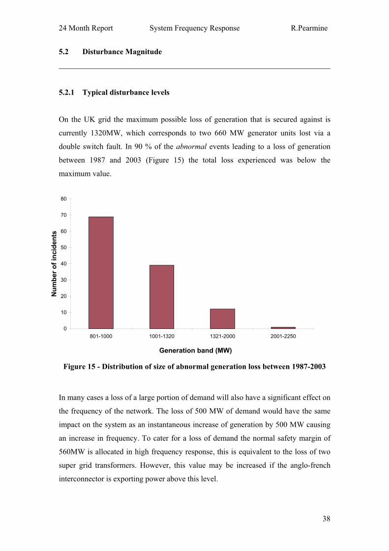
24 Month Report System Frequency Response R.Pearmine
38
5.2 Disturbance Magnitude
5.2.1 Typical disturbance levels
On the UK grid the maximum possible loss of generation that is secured against is
currently 1320MW, which corresponds to two 660 MW generator units lost via a
double switch fault. In 90 % of the abnormal events leading to a loss of generation
between 1987 and 2003 (Figure 15) the total loss experienced was below the
maximum value.
Figure 15 - Distribution of size of abnormal generation loss between 1987-2003
In many cases a loss of a large portion of demand will also have a significant effect on
the frequency of the network. The loss of 500 MW of demand would have the same
impact on the system as an instantaneous increase of generation by 500 MW causing
an increase in frequency. To cater for a loss of demand the normal safety margin of
560MW is allocated in high frequency response, this is equivalent to the loss of two
super grid transformers. However, this value may be increased if the anglo-french
interconnector is exporting power above this level.
0
10
20
30
40
50
60
70
80
801-1000 1001-1320 1321-2000 2001-2250
Generation band (MW)
Nu
mb
er
of
incid
en
ts

24 Month Report System Frequency Response R.Pearmine
39
Depending on the time of day and the time of year system demand levels are usually
between 18GW and 55GW. Figure 16 places a generation loss of 1320MW at
between 6.6 and 2.4 % of the national demand depending on when the event occurs,
this is a significant portion of the total power.
Figure 16 - Typical Grid Demand levels
5.2.2 Disturbance Simulations
Using the same example as in section 4.2.4, it is possible to observe how the
magnitude of the disturbance effects the system response. The curves in Figure 17
show the frequency transients at various loss levels. The deficit of power has a direct
relation to the maximum deviation, steady state value and initial decay rate of the
system frequency as can be seen from the graph.
30
130
230
330
430
530
630
730
830
930
103
0
113
0
123
0
133
0
143
0
153
0
163
0
173
0
183
0
193
0
203
0
213
0
223
0
233
0
Winter Maximum
Typical Winter
Typical Summer
Summer Minimum
15000
20000
25000
30000
35000
40000
45000
50000
55000
Dem
and (
MW
)
Time

24 Month Report System Frequency Response R.Pearmine
40
Figure 17 - Effect of disturbance magnitude on system frequency
49.4
49.5
49.6
49.7
49.8
49.9
50
50.1
0 10 20 30 40 50 60
Time - Seconds
Fre
qu
en
cy
- H
z
1200 MW
1000 MW
800 MW
600 MW

24 Month Report System Frequency Response R.Pearmine
41
5.3 Generator inertia
5.3.1 Effects of inertia
According to Newton’s laws of motion all objects resist changes in their state of
motion. Inertia is the tendency of an object to resist changes in motion and is
dependent upon mass of the object. If we consider a simple generator with angular
rotation ( ) it has inertia (J) acting against the changing motion and a mechanical
driving torque ( M) supplied by a turbine with its counter acting electrical torque ( E).
Machowski(1998) gives this relationship as Equation 6.
EMdt
dJ .
Equation 6
The inertia of a generator is usually normalised as a per unit inertia constant, defined
as the kinetic energy at rated speed over the MVA base. The units of the inertia
constant are seconds, which represents the time it would take to provide the
equivalent amount of stored kinetic energy held in the generator at rated output.
Multiplying the terms in Equation 6 by the normalised speed we have a fundamental
description of the rotor dynamics called the swing equation (Equation 7). The
difference in mechanical power (PM) and electrical power (PE) is solely related to the
inertia and rate of change of rotation.
EM PPdt
dH .2
Equation 7
A typical thermal generator with 2-poles will have an inertia constant (H) that can
range between 2.5 and 6, whilst 4-pole machines have an inertial constant in the order
of 4 to 10. Hydro units are normally smaller and so have typical inertia constants of 2
to 4. On the UK grid the inertial values of the individual generators vary between 9.5
and 3.2.

24 Month Report System Frequency Response R.Pearmine
42
The system inertia as a whole encompasses the inertia of each individual generator
connected to the grid. It can be calculated from the weighted average of the all the
generators operating on the grid at that particular instant. Scheduling generators in
much the same way as with system droop can effect the overall system inertia. By
operating more generators the system inertia is raised. It is also worth remembering
the load is composed of a percentage of similar rotating machines, albeit of a
somewhat smaller scale. These machines will also carry a certain amount of kinetic
energy because of their nature, which contributes to resist any change in frequency.
5.3.2 Inertia simulations
System inertia is the main factor that controls the drop in frequency in the two-second
period before governor action beings to increase generator output. The example from
section 4.2.4 is again used to show inertia properties in Figure 18. Inertia controls the
initial decay of frequency, and has a slight influence on the maximum frequency
deviation and the time of the maximum deviation. However, its impact is not as
significant as for previous parameters.
Figure 18 - Effect of inertia on system frequency
49.4
49.5
49.6
49.7
49.8
49.9
50
50.1
0 10 20 30 40 50 60
Time - Seconds
Fre
qu
en
cy -
Hz
3 MW.MVA-1
4 MW.MVA-1
5 MW.MVA-1
7 MW.MVA-1

24 Month Report System Frequency Response R.Pearmine
43
5.4 Load Frequency Sensitivity
5.4.1 Load Frequency Characteristic
The total system load is composed of elements of both resistive and inductive load.
During an imbalance in generation a net change in load will occur with respect to
frequency. This change is due mainly to motor loads, which typically utilise 40 to 60
percent of the network power and will dominate the load-frequency characteristic of
the system. A motor load is dependent on the voltage and frequency of the power
system to which it is attached. If the system voltage or frequency declines, the
connected motor load magnitude will also decline.
Changes in the system frequency have a larger impact on motor load than deviations
in the voltage, Welfonder et al. (1993). Looking simply at the frequency impact of the
motor load an approximate rule of thumb is that the connected motor load magnitude
will decrease by 2% if the frequency decreases by 1%. To account for the influence of
system loads on frequency a load-frequency characteristic (KL) relates the two
quantities, Equation 8.
0
L
L
L
f
fK
P
P
Equation 8
5.4.2 Load Frequency simulations
The load frequency sensitivity has a considerable influence over the maximum
frequency deviation experienced by the system. The example from section 4.2.4 is
used to show that a system with a higher load-sensitivity characteristic has a smaller
deviation in frequency, Figure 19.

24 Month Report System Frequency Response R.Pearmine
44
49.1
49.2
49.3
49.4
49.5
49.6
49.7
49.8
49.9
50
50.1
0 10 20 30 40 50 60
Time - Seconds
Fre
qu
en
cy
- H
z
2.0 %
0.0 %
0.5 %
1.0 %
1.5 %
Figure 19 - Effect of load sensitivity on system frequency

24 Month Report System Frequency Response R.Pearmine
45
5.5 Scheduling Generator Response
The purpose of response and reserve holding are to provide assurance that foreseeable
levels of generation failure, shortfall or demand forecast error do not cause
involuntary demand disconnection or in worst case system collapse. The allocation of
response is an important factor in power systems operation as it determines the shape
of the generation characteristic.
Response can be defined as the autonomous reaction to frequency deviation and is
required to manage instantaneous imbalances between generation and demand. The
response of the generators is grouped by National Grid into one of three categories:
Primary response for fast (seconds) under frequency regulation, Secondary response
(minutes) to recover the system frequency within operational limits, and High
frequency response the equivalent over frequency regulation (on both time scales).
These response types enable National Grid to artificially group generators according
to their specific transient response characteristics.
Response can be dynamically delivered continuously by part loaded generation
operating under governor action or non-dynamic delivered at set frequency trigger
points, predominantly provided by demand-side management or fast start gas turbines.
Response is held based on the magnitude of the largest generation supply and secured
demand. The response is then offset against the contribution of system inertia and
reaction of demand to changing frequency. Generally speaking, as more generation is
synchronised to meet increasing demand the disturbance becomes a smaller
proportion of the system power, and the system load has more stored kinetic energy in
rotating machines meaning less response is required to contain the same disturbance.
In Great Britain dynamic response is provided by de-loaded generators or Balancing
Mechanism Units (BMUs). These units may be instructed to operate in either a
Limited Frequency Sensitive Mode or a Frequency Sensitive Mode. A BMU
operating in the limited frequency sensitive mode will be considered as frequency
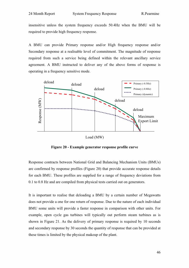
24 Month Report System Frequency Response R.Pearmine
46
insensitive unless the system frequency exceeds 50.4Hz when the BMU will be
required to provide high frequency response.
A BMU can provide Primary response and/or High frequency response and/or
Secondary response at a realisable level of commitment. The magnitude of response
required from such a service being defined within the relevant ancillary service
agreement. A BMU instructed to deliver any of the above forms of response is
operating in a frequency sensitive mode.
Figure 20 - Example generator response profile curve
Response contracts between National Grid and Balancing Mechanism Units (BMUs)
are confirmed by response profiles (Figure 20) that provide accurate response details
for each BMU. These profiles are supplied for a range of frequency deviations from
0.1 to 0.8 Hz and are compiled from physical tests carried out on generators.
It is important to realise that deloading a BMU by a certain number of Megawatts
does not provide a one for one return of response. Due to the nature of each individual
BMU some units will provide a faster response in comparison with other units. For
example, open cycle gas turbines will typically out perform steam turbines as is
shown in Figure 21. As the delivery of primary response is required by 10 seconds
and secondary response by 30 seconds the quantity of response that can be provided at
these times is limited by the physical makeup of the plant.
Res
po
nse
(M
W)
Load (MW)
Maximum
Export Limit
deload
deload
deload
deloaddeload Primary (-0.5Hz)
Primary (-0.8Hz)
Primary (dynamic)

24 Month Report System Frequency Response R.Pearmine
47
Standing Reserve, is carried by contract to cover short notice plant loss and demand
forecasting errors. Following an event that leads to the delivery of response,
instructions are given to standing reserve units to recover the level of response
holding on the system so that BMUs can be brought back to their respective response
holding levels.
Figure 21 - Generator response to applied test frequency injection signal
-5%
0%
5%
10%
15%
20%
25%
30%
35%
0 5 10 15 20 25 30 35 40 45 50 55 60
Time - seconds
% C
han
ge in
Ou
pu
t
HYDRO 1% Droop OCGT CCGT COAL OIL HYDRO 4% droop

24 Month Report System Frequency Response R.Pearmine
48
5.6 Generators for frequency response
5.6.1 Thermal Plant
Generation plant take advantage of several different forms of energy transfer ranging
from traditional coal burning types to modern fuel cell technologies. In all cases a fuel
is oxidised to release energy which is then transported to the required load. Every
single type of generating set operates with slightly different dynamic properties. The
individual plant properties will collectively affect the dynamic response of the system.
For this reason knowledge of how the different plant types operate is essential for
evaluation of frequency stability.
5.6.1.1 Nuclear Stations
In the UK it is typical operating practise to keep nuclear stations running at a constant
power output. This is because of safety concerns with nuclear power; as such they
contribute no responsive generation to the system. Some nuclear plant in the UK is
configured to provide response if necessary although as explained it has never been
called upon to do so.
5.6.1.2 Coal and Oil-fired Stations
In coal-fired stations pulverised fuel is blown into the furnace where it mixes with air
and combusts. In the case of an oil-fired station the oil is combusted in a similar
process.
Steam is produce from the burning of the primary fuel source in either drum or once-
through boilers. Drum boilers, Figure 22a, rely on convection or forced circulation to
transfer heat from the furnace walls, to water. In these boilers the steaming rate is a
direct function of the heat absorbed in the furnace (i.e. the fuel-firing rate). Drum
boilers can still deliver power without any fuel flow into the furnace because of the
quantity of stored heat in the water/steam. This system operates at subcritical

24 Month Report System Frequency Response R.Pearmine
49
pressures relying on a density difference between the steam and water phases for
circulation.
Figure 22 - Typical steam boiler arrangements used in power stations
Once-through boilers, Figure 22b, do not re-circulate water within the furnace;
instead, water is feed at pressure into the furnace tubes by a feed pump. The steaming
rate for this type of boiler is controlled solely by the feed pump. Since this system
does not rely on a density change between steam and water it can operate at
supercritical pressures increasing efficiency. A once-through boiler has less stored
energy than a similar drum boiler unit, and so it is more responsive to changes in
boiler firing.
5.6.1.3 Biofuels
Biofuels are produced from waste vegetable matter or are specifically grown from fast
growing, high yield crops. Biofuels can contribute to electrical production by two
routes, direct burning in a furnace to raise steam or following fermentation in a bio
Boiler feed
pump
Boiler feed
pump
Heat from
Furnace
Heat from
Furnace
Mud
drum
Steam
drum
Steam to
superheaters
Steam
Circulation
a) Drum boiler b) Once-through boiler

24 Month Report System Frequency Response R.Pearmine
50
digester. In either case the method of electrical generation is similar to coal or oil-
fired stations.
5.6.2 Steam Turbines
The high pressure, high temperature steam typically from the boilers is feed into sets
of axial flow turbines. As the steam passes through the turbines or ‘stages’ it loses
pressure and expands in volume. Between stages the steam can be taped of and
reheated to increase operating efficiency.
HP LPLP G
Crossover
Condenser
MSV
CV
To Power
system
FromMSV – Emergency stop valve
CV – Control valve
G – Generator
HP – High pressure turbine
IP – Intermediate pressure turbine
Figure 23 - Non-reheat steam turbine
Steam turbines are categorised by the way in which steam is reheated. Non-reheat
turbines like those in Figure 23 usually have one stage and typically operate below
100 MW. The more common arrangement for high power turbines is a reheat
configuration where up to three stages mean the turbine has a high operating
efficiency. Steam from the boiler passes through the governor control valves and into
the high-pressure stage. After the steam has left this stage it is reheated passes through
more control valves and does more work in the intermediate stage. At the final stage
steam passes from the IP stage by crossover piping for expansion in the low-pressure
turbine where it is finally released as exhaust into a condenser.
With most steam turbine configurations relying on more than one pressure stage less
than 30% of the output power comes from the initial stage. With such a small
proportion of power being extracted from the start of the cycle, reheaters and
crossovers become important components in terms of response. Steam supply through

24 Month Report System Frequency Response R.Pearmine
51
the system cannot be instantaneous; the steam travelling through each of the stages
introduces a finite delay and the dynamic operation of the unit will be influenced.
5.6.3 Gas Turbines
Open cycle gas turbines (OCGT) directly use combustible natural gas in much the
same way as the jet engine on a plane. They are capable of very fast response and start
up times (sub three minutes) and are readily employed on emergency low frequency
trip relays. A turbine diagram is given in Figure 24, a compressor forces air into a
combustion chamber where it mixes with the fuel and ignites. The high pressure, high
temperature gases then drive the turbine stage and exhaust is used to pre heat
incoming air. The gas turbine drive shaft is connected to the generator to provide the
necessary torque for electrical generation.
Figure 24 - Diagram of a simple gas turbine
In recent years the CCGT or combined cycle gas turbine has become increasingly
dominant in the industry. It uses heat recovered from the gas combustion process to
raise steam, which can then be used to drive an addition steam turbine. The steam
raised from a typical gas turbine is only sufficient to support a steam turbine unit of
half its capacity.
For this reason two distinct plant configurations have evolved.
Single shaft machines, which have a gas and steam turbine (half the GT rating) on
the same drive shaft Figure 25
Air
intake
Combustion
Chamber
Compressor
Exhaust
Fuel
Turbine

24 Month Report System Frequency Response R.Pearmine
52
Multi shaft plant in which a steam turbine and two gas turbines drive individual
generators that are mechanically isolated from each other. Figure 26
Figure 25 - Single shaft tandem plant configuration
Figure 26 - Multi-shaft plant configuration
Multi-shaft configurations are the most common arrangements to be found connected
to the UK grid because they were initially favoured. Newer plant tends to be of the
LPLP G
Condenser
To
Power
system
HP
GTCP
FuelAir
Exhaust
CV
GTCP G
G
To
Power
system
To
Power
system
LPLP G
Condenser
To
Power
system
HPGTCP
Fuel
Air
Exhaust
CV CV
CP – Compressor
GT – Gas Turbine
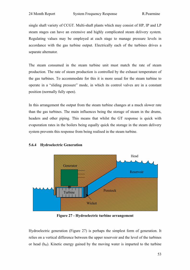
24 Month Report System Frequency Response R.Pearmine
53
single shaft variety of CCGT. Multi-shaft plants which may consist of HP, IP and LP
steam stages can have an extensive and highly complicated steam delivery system.
Regulating values may be employed at each stage to manage pressure levels in
accordance with the gas turbine output. Electrically each of the turbines drives a
separate alternator.
The steam consumed in the steam turbine unit must match the rate of steam
production. The rate of steam production is controlled by the exhaust temperature of
the gas turbines. To accommodate for this it is more usual for the steam turbine to
operate in a “sliding pressure” mode, in which its control valves are in a constant
position (normally fully open).
In this arrangement the output from the steam turbine changes at a much slower rate
than the gas turbines. The main influences being the storage of steam in the drums,
headers and other piping. This means that whilst the GT response is quick with
evaporation rates in the boilers being equally quick the storage in the steam delivery
system prevents this response from being realised in the steam turbine.
5.6.4 Hydroelectric Generation
Figure 27 - Hydroelectric turbine arrangement
Hydroelectric generation (Figure 27) is perhaps the simplest form of generation. It
relies on a vertical difference between the upper reservoir and the level of the turbines
or head (hH). Kinetic energy gained by the moving water is imparted to the turbine
Generator
Penstock
Reservoir
Turbine
Wicket
Head

24 Month Report System Frequency Response R.Pearmine
54
blades, which are used to drive generators. The generator power (PG) available can be
calculated from Equation 9.
WhgWhP wG 81.9H H
Equation 9
The output power is derived from the water density ( w), acceleration due to gravity
(g) and water flow rate (W) through the turbine, which is dependent on the specific
design of the system. Detailed representation of turbine design, penstock, surge tanks,
water column dynamics and travelling wave effects may be necessary to provide an
accurate model of the hydro generator.
Figure 28 - Dinorwig Hydroelectric pumped storage facility
Scotland operates approximately 200MW of cascade hydro schemes. In England and
Wales the hydroelectric generation is mainly utilised in pumped storage facilities such
as Ffestiniog and Dinorwig (Figure 28). At these stations water is pumped into a large
reservoir during periods of low demand. This store can be released on request and is
capable of supplying up to 6 hours of full load generation. The quality of response
that can be provided by these machines means that the plant is well suited to use as a
fine frequency control tool.
Headworks
Lowwater level

24 Month Report System Frequency Response R.Pearmine
55
5.6.5 Wind Power
Wind farms provide the most economically feasible source of large-scale renewable
generation. The largest development to date is a 60 MW facility operating at North
Hoyle Figure 29. Theoretically the maximum power that can be obtained from wind
generation is dependant on air density ( a), wind speed (uw) and swept area of the
turbine blades (Aw), Equation 10.
3
2
1uAP waG w
Equation 10
Operation of the wind turbines is only possible at wind speeds above a critical point,
usually between 3 and 5 ms-1
. The developed power increases with wind speed until
the rated output is attained. At rated power blade pitch is altered or the turbine is
allowed to stall so as to maintain a constant output with further increase in wind
speed. The generators also have a maximum operational speed (typically 20 ms-1
),
which if breached causes the generator to shut down.
Figure 29 - North Hoyle offshore wind installation
Wind turbines are typically composed of small-scale induction generators with
outputs in the order of 2 MW. To reach the required capacity, individual windmills
are connected to the grid in banks via transformer sub-stations to create wind farms.
The fixed speed types rely on rotor stall to limit the power output at high wind speeds.
Typically, variable-speed turbines use aerodynamic blade pitch controls in
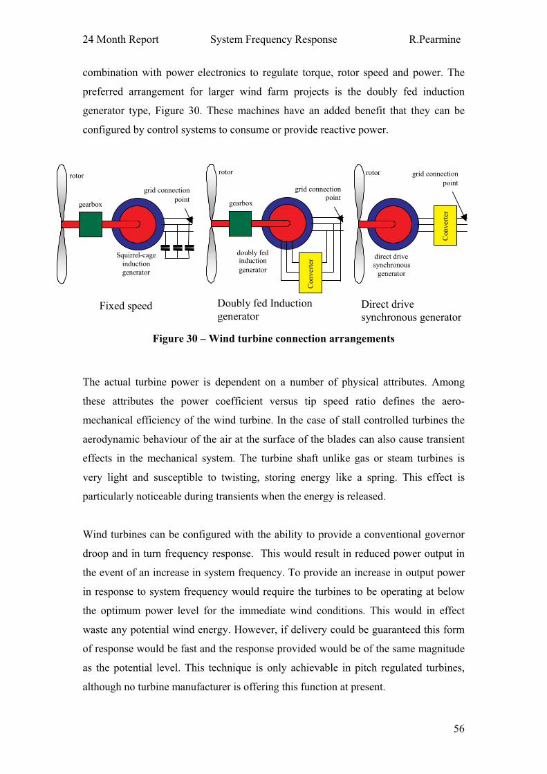
24 Month Report System Frequency Response R.Pearmine
56
combination with power electronics to regulate torque, rotor speed and power. The
preferred arrangement for larger wind farm projects is the doubly fed induction
generator type, Figure 30. These machines have an added benefit that they can be
configured by control systems to consume or provide reactive power.
Figure 30 – Wind turbine connection arrangements
The actual turbine power is dependent on a number of physical attributes. Among
these attributes the power coefficient versus tip speed ratio defines the aero-
mechanical efficiency of the wind turbine. In the case of stall controlled turbines the
aerodynamic behaviour of the air at the surface of the blades can also cause transient
effects in the mechanical system. The turbine shaft unlike gas or steam turbines is
very light and susceptible to twisting, storing energy like a spring. This effect is
particularly noticeable during transients when the energy is released.
Wind turbines can be configured with the ability to provide a conventional governor
droop and in turn frequency response. This would result in reduced power output in
the event of an increase in system frequency. To provide an increase in output power
in response to system frequency would require the turbines to be operating at below
the optimum power level for the immediate wind conditions. This would in effect
waste any potential wind energy. However, if delivery could be guaranteed this form
of response would be fast and the response provided would be of the same magnitude
as the potential level. This technique is only achievable in pitch regulated turbines,
although no turbine manufacturer is offering this function at present.
gearbox
rotor
grid connection
point
Squirrel-cage
induction
generator
Conv
erte
r
gearbox
rotor
grid connection
point
doubly fedinduction
generator
Conv
erte
r
rotor grid connection
point
direct drive
synchronous
generator
Fixed speed Doubly fed Induction
generatorDirect drive
synchronous generator

24 Month Report Work to Date R.Pearmine
57
6 Work to Date
6.0 Modelling Objectives
The most critical objective of the research is to formulate a response requirement that
does not breach National Grid guidelines on security and quality of supply. Any loss
of demand or generation should not allow frequency to deviate from the nominal by
more than 0.5Hz in losses below 1000MW, or 0.8Hz for those 1000-1320MW.
The research should develop a tool to investigate the effect changing system
parameters has on system frequency. This tool should provide the added functionality
to accommodate various future scenarios. Such scenarios may include losses above
1320 MW (as the system is further stressed by increased electrical demand); or
increased penetration of wind turbines.
Chapter 5 detailed some of the more important characteristics that affect frequency
response. Of particular significance to achieving an accurate frequency transient after
modelling a loss event is selection of an accurate value of load sensitivity. By
quantifying the load frequency characteristic on the GB grid this will be achieved.
Further optimisation of the response requirement would be possible if daily/seasonal
trends can be established in the load frequency characteristic. This could reduce the
response holding requirement.
The system frequency was shown in Chapter 5 to be heavily dependent on the power
balance. To ensure the accuracy of simulations all components relating to electrical
power which principally includes turbine governor models should be as accurate as
possible.

24 Month Report Work to Date R.Pearmine
58
6.1 Load Behaviour
The Load-frequency characteristic is determined by consumer behaviour, which
makes direct comparisons between other networks and GB difficult. National Grid
currently uses a value of 2 %/Hz for its load-frequency sensitivity, which has been
developed through operating practice and confidence in the system security. Many
literature sources quote the load sensitivity factor as a percentage value, which is
normalised against base frequency and system power. However, we will hold with
convention adopted by National Grid and quote sensitivity in % reduction per Hz
deviation.
The Irish electricity grid calculates load sensitivity to frequency O’Sullivan and
O’Malley(1996) in the order of 2-2.5 %/Hz. The UCPTE, Weber et al.(1997), gives
values for the load sensitivity in the order of 0.8-3.3 %/Hz. Tests carried out by
Berg(1972) on an isolated power system in Norway show average values of load
sensitivity as 1.0 %/Hz for commercial loads and 0.8 %/Hz for a residential load, the
paper notes however that a great deal of variation was evident when calculating the
average values. Concordia and Ihara(1982) provide details of measured load
characteristics from New York in the years 1941 and 1969 as 3.0 to 3.2 %/Hz and 3.0
to 4.0 % respectively. Näser and Grebe(1996) use a value of 2 % /Hz in their paper
discussing the cost of reserve.
Schulz(1999) assumed the load characteristic of the Eastern Interconnector in
America. to be 2.5%/Hz. NEMMCO(2002) has estimated that the power system
demand varies with frequency at 2.5 %/Hz. A report published by Chown and
Coker(2000) for Eskom gives an average load frequency characteristic of 2.5 %/Hz.
Figures published by an IEEE task force on load representation(1993) give frequency
sensitivity for residential loads as 1.4–2.0 %/Hz differing from those suggested by
Concordia by at least 50%. This discrepancy may be due to the change in load mix
within the ten-year period. Commercial loads are determined to be between 2.0-2.8
%/Hz, with industrial loads 2.2 %/Hz, Aluminium refineries -0.5 %/Hz, Steel Mills
2.5 %/Hz, Power Aux. Plant 4.8 %/Hz, and Agricultural Pumps 9.3%/Hz.

24 Month Report Work to Date R.Pearmine
59
Welfonder et al.(1989) provide results from load dependency tests carried out on parts
of the German grid system. The Load-frequency characteristic is evaluated as 2.4
%/Hz at Heidelberg and 1.6 %/Hz at Berlin. The difference at the sites is attributed to
a higher constituent of motor load in the Heidelberg area. A supplementary paper was
also published in 1993 giving details of a further six areas with seasonal
dependencies.
KL
(%MW/Hz)
or
(%MW/%Hz)
NGT 2 2.86 – 8.89
Ireland 2 – 2.5 -
UCPTE 0.8 – 3.3 6.7 - 9.6
Norway 0.8 - 1 -
New York 3 - 4 -
America (Eastern Interconnection)
2.5 3.9 - 4.4
NEMMCO 2.5 -
South Africa 2.5 -
Germany 2 -
Germany (part system) 1.6 - 2.4 -
Table 2 - Sensitivity Factors and Power-frequency characteristics
In summary the load characteristic is typically represented as a value between 0.8 and
4 %/Hz, Table 2 summarises the characteristic values given in this section. This large
variation in accepted values suggests that further investigation into the load frequency
sensitivity is required in order to refine our understanding.

24 Month Report Work to Date R.Pearmine
60
6.2 Load Behaviour on the GB grid
Methods have been developed in various countries to quantify a value of load-
frequency sensitivity. Hayashi(1988), Davies et al.(1958) and Fukuda et al.(1989) use
tie lines to measure frequency response across two isolated systems. Welfonder et
al.(1993) measure load characteristics on feeders of small part systems. All these
techniques have a similar drawback in that they can only consider part of the system
in question. A global sensitivity figure must be scaled up from the part system
response and is a source for error.
As part of National Grids data archive it has been continuously recording historical
demand and generation values from the network at intervals of one minute since June
1993. However, to quantify the load-frequency sensitivity on the UK grid this data
has not been of the resolution needed to capture the dynamic changes of the system.
As a consequence a piece of software was developed to allow the continuous logging
of an existing real-time data channel at intervals of between 2-10 seconds. With this
data it is possible to evaluate the frequency response of the load to a much higher
accuracy.
Although not a direct account of demand the technique uses the recorded change in
grid-connected generation ( PG) and the loss of a known generation (PLoss) to
calculate the power attributed to demand sensitivity (kpf), Equation 11.
PL = PG - PL - PG = PLoss - PG = kpf. F
Equation 11
Unfortunately, this method requires an instantaneous loss of generation (or increase in
load) of a significant magnitude to take place. During operation it has been found that
a disturbance greater than 200 MW provides an adequate power mismatch to measure
the load sensitivity although higher levels are desirable. From recent incidents it has
been possible to calculate a value for the load-frequency sensitivity; Figure 31.

24 Month Report Work to Date R.Pearmine
61
0
1
2
3
4
5
6
01-Jun-04 01-Jul-04 31-Jul-04 30-Aug-04 29-Sep-04 29-Oct-04 28-Nov-04 28-Dec-04
Date of Incident
Lo
ad
sen
sit
ivit
y %
/Hz
Equation 11 Equation 12
Figure 31 – Recorded Load sensitivity to frequency on the GB system
The weakness of using Equation 11 to calculate demand change, is it requires a steady
demand to gain meaningful results. Figure 32 and Figure 33 highlight this weakness
with data under a stable demand compared with an increasing demand, which is
unpredictable from the generation trace alone.
To corroborate the results a second method was also used involving the initial rate of
change of system frequency at the onset of an event, Inoue et al.(1999). Using this
initial decay rate, the total load and also the system inertia it is possible to calculate
the power mismatch between load and generation ( P). The formula is given in
Equation 12.
0
2.
H d fP
f dt
Equation 12
The results using this method are however very sensitive to the initial value of
frequency decay (which is only recorded to one-second resolution).
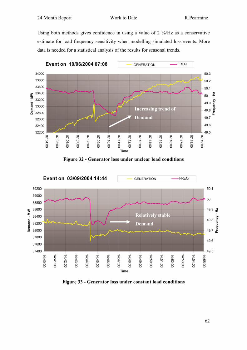
24 Month Report Work to Date R.Pearmine
62
Using both methods gives confidence in using a value of 2 %/Hz as a conservative
estimate for load frequency sensitivity when modelling simulated loss events. More
data is needed for a statistical analysis of the results for seasonal trends.
Figure 32 - Generator loss under unclear load conditions
Figure 33 - Generator loss under constant load conditions
Event on 03/09/2004 14:44
37400
37600
37800
38000
38200
38400
38600
38800
39000
39200
14
:40
:00
14
:41
:00
14
:42
:00
14
:43
:00
14
:44
:00
14
:45
:00
14
:46
:00
14
:47
:00
14
:48
:00
14
:49
:00
14
:50
:00
14
:51
:00
14
:52
:00
14
:53
:00
14
:54
:00
14
:55
:00
Time
De
man
d -
MW
49.5
49.6
49.7
49.8
49.9
50
50.1
Fre
qu
en
cy -
Hz
Tot_DemMW FREQ
Relatively stable
Demand
GENERATION
Event on 10/06/2004 07:08
32200
32400
32600
32800
33000
33200
33400
33600
33800
34000
07:0
4:0
0
07:0
5:0
0
07:0
6:0
0
07:0
7:0
0
07:0
8:0
0
07:0
9:0
0
07:1
0:0
0
07:1
1:0
0
07:1
2:0
0
07:1
3:0
0
07:1
4:0
0
07:1
5:0
0
07:1
6:0
0
07:1
7:0
0
07:1
8:0
0
07:1
9:0
0
Time
Dem
an
d -
MW
49.5
49.6
49.7
49.8
49.9
50
50.1
50.2
50.3
Fre
qu
en
cy -
Hz
Tot_DemMW FREQ
Increasing trend of
Demand
GENERATION

24 Month Report Work to Date R.Pearmine
63
6.3 Generator Behaviour on the GB grid
We saw in chapter 5 that generator droop and generator transient response also has a
large impact on the frequency transient, both are inherent in the governor model.
From the first studies used to calculate primary response requirement,
Williams(2003), it was believed that the response provided by generator models was
higher than was to be expected. After investigations comparing individual gas and
coal-fired generators on a simple network this project had shown that the generator
did seem to be providing marginally more response but not in all cases Figure 34 and
Figure 35.
Figure 34 - Simulation of CCGT turbine at deload of 110 MW
Figure 35 – Simulation of coal fired steam turbine at deload of 95 MW
640
650
660
670
680
690
700
710
-10 0 10 20 30 40 50 60 70 80 90 100
Time - seconds
Ou
tpu
t -
MW
On siteGenerator Test
Governormodel
Contract Data0.2Hz frequency
Injection
540
555
570
585
600
615
630
645
660
-10 0 10 20 30 40 50 60 70 80 90 100 110 120
Time - Secs
Ou
pu
t -
MW
On siteGenreatorTest
Govenor(includingboilerdydnamics)
SimpleGovenor
ContractData
0.2Hz frequency
Injection
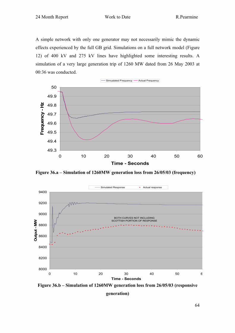
24 Month Report Work to Date R.Pearmine
64
A simple network with only one generator may not necessarily mimic the dynamic
effects experienced by the full GB grid. Simulations on a full network model (Figure
12) of 400 kV and 275 kV lines have highlighted some interesting results. A
simulation of a very large generation trip of 1260 MW dated from 26 May 2003 at
00:36 was conducted.
Figure 36.a – Simulation of 1260MW generation loss from 26/05/03 (frequency)
Figure 36.b – Simulation of 1260MW generation loss from 26/05/03 (responsive
generation)
49.3
49.4
49.5
49.6
49.7
49.8
49.9
50
0 10 20 30 40 50 60
Time - Seconds
Fre
quency - H
z
Simualated Frequency Actual Frequency
8000
8200
8400
8600
8800
9000
9200
9400
0 10 20 30 40 50 6
Time - Seconds
Outp
ut - M
W
Simulated Response Actual response
BOTH CURVES NOT INCLUDING
SCOTTISH PORTION OF RESPONSE

24 Month Report Work to Date R.Pearmine
65
Figure 36.c – Simulation of 1260MW generation loss from 26/05/03 (non-
responsive generation)
This simulation showed that the generator response (Figure 36.b) to a 0.54 Hz
frequency deviation was much greater in the model than in the real event. Post event
reports show that 15% of generators failed to supply Primary response (approximatley
70 MW), but this still does not account for the 400 MW difference.
By using data collected from the demand logging system it became possible to get
cumulative generation totals of the various types of generator. By simulating another
generator loss and comparing the simulated response to the recorded response it is
possible to see which generator type is contributing to the inaccuracies. The largest
generator loss recorded to date was taken as the test simulation. This was the loss of
615 MW generation on 16 August 2004 at 19:04.
The results given in Figure 37 and Figure 38 show that despite a small discrepancy in
the initial levels of the generation, the response of the CCGT turbines is far greater in
the simulation that those experienced on the network. In fact, the gas turbines in this
case produce a 250 MW peak of response. Coal units also produce a faster response in
the simulation compared to real-time data.
14400
14600
14800
15000
15200
15400
15600
15800
0 10 20 30 40 50 6
Time - Hz
Ou
tpu
t -
MW
Simulated Non-Response

24 Month Report Work to Date R.Pearmine
66
Other network operators, Nagpal et al(2001), have raised concerns over the use of a
similar OCGT model in simulations. The chief issue is with regard to the inability of
the model to fully represent temperature control when put into a CCGT mode of
operation. The temperature control loop limits power outputs at full load, which is
particularly relevant for responsive plant during large frequency deviations. This
establishes the need for a specific CCGT model to represent the combined cycle
turbines.
All of the plant models used in the simulations are taken from previous transmission
study models. Recent discussions with NGT staff revealed that the models used in
transmission studies are generic plant models only. They only represent the minimum
performance requirement as specified in the Grid Code. This raises the need to review
the existing models currently in use against representative real machine data as was
confirmed by the simulations from 26/05/03 and 16/08/04.
With an increased confidence in the validated thermal plant models a wind turbine
model will be required. Several possible models exist including a generic model
developed by Eurostag(2004). The chosen model will require validation in a similar
manner to the thermal models, against actual real-time data to ensure its accuracy.

24 Month Report Work to Date R.Pearmine
67
Figure 37 – Simulation of 615MW
Generator loss on 16/09/04
Figure 38 – Network response to 615MW
Generator loss on 16/09/04
Fre
quen
cy
Pow
er O
utp
ut
MW
0
200
400
600
800
1000
1200
1400
12000
12200
12400
12600
12800
13000
13200
13400
13600
13800
14000
14200
EDF SCP OTHER COAL CCGT NUC OMEGA
19:0
4:3
9
19:0
4:4
9
19:0
4:5
9
19:0
5:0
9
19:0
5:1
9
19:0
5:2
9
19:0
5:3
9
6400
6600
6800
49.9
49.95
50
50.05
50.1
50.15
50.2
0 10 20 30 40 50 60

24 Month Report Work to Date R.Pearmine
68
6.4 Future Work
The following paragraphs highlight the work that is to be concluded over the next 2
years of the research project. The timescales of each individual task are shown
diagrammatically in the Gantt chart of section 6.5, also showing relevant submission
dates and course modules.
1. Validate steam turbine models against individual plant
As was discussed in chapter 6.2, there is a need to validate existing models of coal,
and oil fired plant against actual frequency deviations. This task will use recorded
frequency traces from past events to be injected into governor models of frequency
responsive plant. The resulting power output simulated by the models can then be
verified against the recorded responses during the event. The models can be adjusted
where necessary until a satisfactory representation is achieved.
2. Develop CCGT model against individual plant
In chapter 6.2 issues were raised over the suitability of OCGT models for
representing CCGT plant. After reviewing current operating practises and literature
on CCGT machines a model to simulate frequency response will be presented. As in
the previous task validation of the model against actual frequency deviations is
required. This will require following the same methodology as was the case for coal
plant.
3. Review existing incidents using validated models
With confidence in the individual thermal plant models (established through tasks 1
and 2), a set of full network simulations can be carried out. This will entail several
simulations like those of chapter 6.2 whereby a specific plant loss is represented fully
across every component of the network. This will verify the robustness of the network
model components, and the simplification of only using 275kV and 400kV nodes.

24 Month Report Work to Date R.Pearmine
69
4. Add Scottish nodes to grid model
With the onset of BETTA in April 2005, NGT will increase its control operations to
include Scotland. Previously Scotland was represented as a lumped element as it did
not benefit studies to include the full load and generator contributions of this part of
the network. As operational issues will soon include the effects of this network
representation should be provided in the network model.
5. Write/Submit paper1
This paper aims to describe the effects of load behaviour on the UK system during
frequency disturbances. It will provide examples of generator loss on the system and
the drop in frequency as a result. It is hope to include details of generator responses
also. This paper will be submitted to the IEEE Transactions in power systems.
6. Review response requirements examining effects of geographic reserve holding
With a full model of the network and accurate governor models it will be possible to
assess the level of response required to contain specific losses within frequency limits.
Simulations of 300MW loss against a -0.2Hz frequency deviation; 600, 700, 800, 900,
1000MW losses against -0.5Hz deviation; and 1100, 1200, 1260 and 1320MW losses
against -0.8Hz deviation will be made. These simulations will be required at demand
levels ranging from 15 to 65GW. The simulations will also investigate the effects (if
any) that result from situating the reserve in a specific geographic area on the grid.
7. Review literature on modelling of wind turbines
In chapter 2 we established that the majority of renewable generation to meet
government targets would come from wind turbines. In order to simulate the effect of
these turbines on the frequency response requirement a model of their control strategy
must be represented in the simulations. Much literature has been published recently
regarding modelling of individual wind turbines and aggregated farms. To provide a
suitable model a review of all current research will be undertaken.
8. Build wind farm model
All grid connected wind farms will be over 50MW in capacity, this results in many
individual wind turbines. With a finite processing ability the model established from
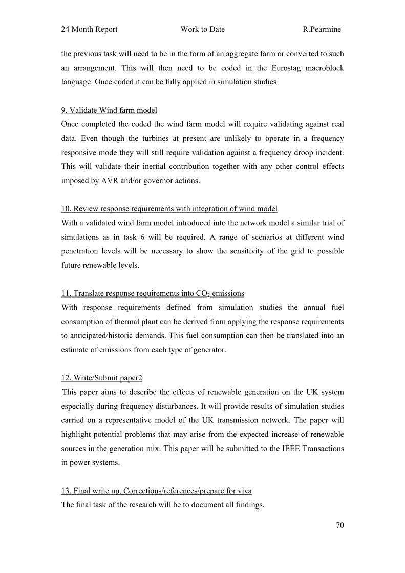
24 Month Report Work to Date R.Pearmine
70
the previous task will need to be in the form of an aggregate farm or converted to such
an arrangement. This will then need to be coded in the Eurostag macroblock
language. Once coded it can be fully applied in simulation studies
9. Validate Wind farm model
Once completed the coded the wind farm model will require validating against real
data. Even though the turbines at present are unlikely to operate in a frequency
responsive mode they will still require validation against a frequency droop incident.
This will validate their inertial contribution together with any other control effects
imposed by AVR and/or governor actions.
10. Review response requirements with integration of wind model
With a validated wind farm model introduced into the network model a similar trial of
simulations as in task 6 will be required. A range of scenarios at different wind
penetration levels will be necessary to show the sensitivity of the grid to possible
future renewable levels.
11. Translate response requirements into CO2 emissions
With response requirements defined from simulation studies the annual fuel
consumption of thermal plant can be derived from applying the response requirements
to anticipated/historic demands. This fuel consumption can then be translated into an
estimate of emissions from each type of generator.
12. Write/Submit paper2
This paper aims to describe the effects of renewable generation on the UK system
especially during frequency disturbances. It will provide results of simulation studies
carried on a representative model of the UK transmission network. The paper will
highlight potential problems that may arise from the expected increase of renewable
sources in the generation mix. This paper will be submitted to the IEEE Transactions
in power systems.
13. Final write up, Corrections/references/prepare for viva
The final task of the research will be to document all findings.
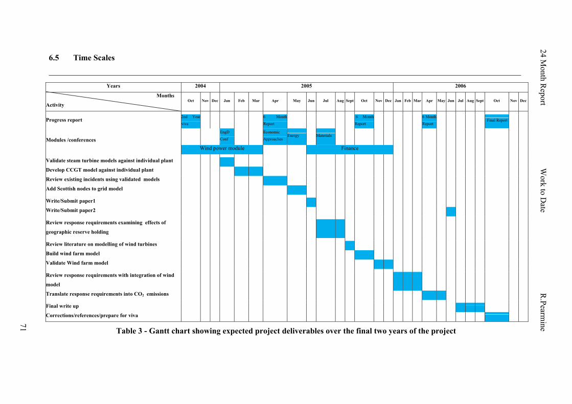
6.5 Time Scales
Table 3 - Gantt chart showing expected project deliverables over the final two years of the project
Years 2004 2005 2006
Months
Activity Oct Nov Dec Jan Feb Mar Apr May Jun Jul Aug Sept Oct Nov Dec Jan Feb Mar Apr May Jun Jul Aug Sept Oct Nov Dec
Progress report 2nd Year
viva
6 Month
Report
6 Month
Report
6 Month
Report Final Report
EngD
Conf
Economic
Approaches Energy Materials
Modules /conferences
Wind power module Finance
Validate steam turbine models against individual plant
Develop CCGT model against individual plant
Review existing incidents using validated models
Add Scottish nodes to grid model
Write/Submit paper1
Write/Submit paper2
Review response requirements examining effects of
geographic reserve holding
Review literature on modelling of wind turbines
Build wind farm model
Validate Wind farm model
Review response requirements with integration of wind
model
Translate response requirements into CO2 emissions
Final write up
Corrections/references/prepare for viva
24 M
onth
Rep
ort
Work
to D
ate R
.Pearm
ine
71

24 Month Report Conclusion R.Pearmine
72
7 Conclusion
7.0 Conclusion
A brief introduction has been given to some of the technical aspects that influence the
frequency response of the network. Details are given of the current operating practices
for frequency control in GB at the present time, together with a selection of other
countries. Frequency responsive generation inherently causes more environmental
impact than base load generation. As such, any efforts to reduce the requirement of
frequency response holding will decrease environmental impact.
A methodology is proposed to study the effects of frequency response on the
transmission grid using a simulation package called Eurostag. The same methodology
will allow its impact to be assessed against an increase in wind power. This will lead
to a better understanding of how the increase in renewable generation will effect the
operation of the transmission system over the next fifteen years.
Current progress has been made in efforts to quantify the Load-Frequency sensitivity
of the GB grid, which will continue. Also, simulations involving generating units
have helped raised issues regarding model accuracy that must be addressed before
further work is possible.
Future work has been discussed with particular attention given to the validation of
models against test data and system events to increase simulation accuracy. The next
stages of the research will see the development of suitable CCGT and wind turbine
model. Once a competent library of models exists it will be possible to assess the

24 Month Report Conclusion R.Pearmine
73
current frequency response requirement. Work can then also begin to quantify the
level of response that would be required given a significant increase in the number of
wind turbines or different system characteristics. This can then be related in terms of
CO2 emissions.

24 Month Report References R.Pearmine
74
8 References
1. Adibi, M. M. and Borkoski, J. N. and Kafka, R. J. and Volkmann, T. L., (May
1999), 'Frequency response of prime movers during restoration'
Power systems, IEEE Transaction on, Vol. 14, No.2 Page(s): 751-756
2. Akhmatov, V. and Knudsen, H. and Nielsen, A. H. and Pedersen, J. K. and
Poulsen, N. K., (2003) 'Modelling and transient stability of large wind farms'
Electrical power and Energy systems, Volume: 25 Page(s): 123 - 144
3. Anderson, P. M. and Mirheydar, M., (Aug. 1999) 'A low-order system frequency
response model'
Power systems, IEEE Transaction on, Vol. 5, No.3 Page(s): 720-729
4. Berg, G.J., (Oct. 1972) 'System and load behaviour following loss of generation'
Proceedings of IEE, Volume: 119 Issue: 10 Page(s): 1483 – 1486
5. Bize, L. N. and Hurley, J. D., (31 Jan-4 Feb. 1999) 'Frequency control
considerations for modern steam and combustion turbines'
Power Engineering Society 1999 Winter Meeting, IEEE ,Volume: 1 Page(s):548 -
553 vol.1
6. Bourles, H. and Colledani, F. and Houry, M. P., (Feb. 1997) 'Robust continuous
speed governor control for small signal and transient stability'
Power Systems, IEEE Transactions on , Volume: 12, Issue: 1 Page(s): 129-134
7. British Wind Energy Association, (Monday 16th September 2002) 'Wind can meet
nuclear shortfall'
http://www.bwea.com/media/news/energyreveiw.html
8. Chan, M. L. and Dunlop, R. and Schweppe, F., (Jan. 1972) 'Dynamic equivalents
for average system frequency behaviour following major disturbances'
IEEE PES winter meeting, New York Page(s): 1-7

24 Month Report References R.Pearmine
75
9. Chown, G. and Coker, M., (Aug. 2000) 'Interim report on frequency relaxation
project', Eskom
http://www.sappstem.com/docs/frequency%20relaxation.pdf
10. Concordia, C. and Ihara, S., (Apr. 1982) 'Load representation in power system
stability studies'
Power Apperatus and Systems, IEEE Transactions on , Volume: PAS-101 Issue: 4
Page(s): 136 – 143
11. Davies, M. and Moran, F. and Bird, J. I., (Nov. 1958) 'Power frequency
characteristics of the British grid system.'
IEE Proceedings Page(s): 154 – 162
12. de Mello, F. P., (Feb. 1991) 'Boiler models for system dynamic performance
studies'
IEEE Power Engineering Review Page(s): 47
13. DTI (2000) 'Energy Paper 68: Energy projections for the UK'
http://www.dti.gov.uk/energy/inform/energy_projections/ep68_final.pdf
14. DTI (2002) 'Renewables Obligation Order (2002)'
http://www.dti.gov.uk/energy/renewables/publications/pdfs/obligation_2002.pdf
15. DTI (Mar. 2002) 'The Severn barrage – definition study of a new appraisal of the
project'
http://www.dti.gov.uk/energy/renewables/publications/pdfs/rpp027.pdf
16. DTI (2004) 'Digest of United Kingdom Energy Statistics 2004'
http://www.dti.gov.uk/energy/inform/dukes/dukes2004/index.shtml
17. Ekanayake J.B., Holdsworth L. and Jenkins N., (Feb 2003),'Control of DFIG
Wind Turbines'
IEE Power Engineer, Volume: 17, Issue: 1 Page(s): 28-32.
24 Month Report References R.Pearmine
76
18. Electricity Asscociation (2003) 'Electricity and the Environment 2003'
http://www.electricity.org.uk/default.asp?action=article&ID=287#elecEnv2002
19. Elkraft, (1996) 'Summary of recommendation for frequency and time deviation'
http://eng.elkraft-system.dk/C1256C790032C72A/(AllDocsByDocId)/F777DBE7
BCBC7D9EC1256ED000440AC1?OpenDocument
20. Eltra, (2003a) 'Annual Report 2003'
http://www.eltra.dk/media(15796,1033)/Annual_Report_2003.pdf
21. Eltra, (2003b) ' Eltra's Purchases of ancillary services and regulating reserves'
http://www.eltra.dk/media(15104,1033)/Eltra's_Purchases.pdf
22. E.ON Netz GmbH, (2004) 'Wind Report 2004'
http://www.eon-energie.de/bestellsystem/files/EON_Netz_Windreport_e_eng.pdf
23. EUROSTAG,(2204) 'Double fed induction machine: a EUROSTAG model'
http://www.eurostag.be/download/windturbine2004.pdf
24. Fukuda, (1989) 'Estimation method of power-frequency characteristic with normal
operating data'
Proceedings IEE of Japan, Power Engineering Conference, PE-89-6 Page(s): 53 -
62 (in Japanese)
25. Hannett, L.N. and Feltes, J.W., (28 Jan.-1 Feb. 2001) 'Testing and model
validation for combined-cycle power plants'
Power Engineering Society Winter Meeting, 2001. IEEE ,Volume: 2 Page(s):664 -
670 vol.2
26. Hayashi, (1988) 'On-line estimation of power-frequency characteristic'
Proceedings IEE of Japan Conference No. 910 Page(s): 1146-1147 (in Japanese)

24 Month Report References R.Pearmine
77
27. IEEE, (Aug. 1992) 'IEEE recommended practice for excitation system models for
power system stability studies'
IEEE Std 421.5-1992
28. IEEE committee report (28 Jan-2 Feb. 1973) 'Dynamic models for steam and
hydro turbines in power system studies'
Power Engineering Society 1999 Winter Meeting, IEEE Page(s): 1904-1915
29. IEEE task force on Load representation for dynamic performance (May 1993)
'Load representation for dynamic performance analysis'
Power Systems, IEEE Transactions on , Volume: 8, Issue: 2 Page(s): 472 – 482
30. Inoue, T. and Ikeguchi Y. and Yoshida, K., (Feb. 1997) 'Estimation of power
system inertia constant and capacity of spinning reserve support generators using
measured frequency transients'
Power Systems, IEEE Transactions on , Volume: 12 Issue: 1 Page(s): 136 – 143
31. Kelly, M. and Cooke, A. and Hope, J. and McNamara, F. and Witmarsh-Everiss,
M.J. and Canning, T.O.M., (Aug. 1994) 'Modelling of post generation loss
frequency behaviour in power systems'
CIGRE session 38-307 Page(s):
32. Kundur, P., (1993) Power system stability and control
Electric Power Research Institute, McGraw-Hill, New York
33. Kunitomi, K. and Kurita, A. and Tada, Y. and Ihara, S. and Price, W.W. and
Richardson, L.M. and Smith, G., (May 2003) 'Modelling combined-cycle power
plant for simulation of frequency excursions'
Power Systems, IEEE Transactions on, Volume: 18 , Issue: 2 Page(s):724 - 729
34. Lindahl, S. (2002), Verification of Governor Response During Normal Operation,
IEEE/PES Summer Meeting, Chicago, USA, 21-25 July 2002.

24 Month Report References R.Pearmine
78
35. Machowski, J. and Bialek, J. W. and Bumby, J. R., (1998) Power system dynamics
and stability
John Wiley & sons, New York
36. Mijailovi , S. V. and Popovi , D. P., (1997) 'Fast evaluation of dynamic changes
of electric power systems frequency during primary control'
Electrical power & energy systems, Volume: 19, Issue: 8 Page(s): 525-532
37. Mummert, C.R., (31 Jan.-4 Feb. 1999) 'Excitation system limiter models for use
in system stability studies'
Power Engineering Society 1999 Winter Meeting, IEEE , Volume: 1 Page(s):187 -
192 vol.1
38. Nagpal, M. and Moshref, A. and Morison, G.K. and Kundur, P., (2001)
'Experience with testing and modeling of gas turbines'
Power Engineering Society Winter Meeting, IEEE ,Volume: 2 , 28 Jan.-1 Feb.
2001 Page(s):652 - 656 vol.2
39. Näser, W. and Grebe, E., (1996) 'Kosten von Regelmaßnahmen im Netzbetrieb'
(in German)
VDI Berichte, NR. 1245 Page(s): 35 - 49
40. National Electricity Market Management Company Limited (15 Jan. 2002)
'Discussion Paper: Generation and Load Measurement'
ACN. 072 010 327, Version No: 1.0
41. Nordel, (2003) 'Annual report 2003'
http://195.18.187.215/Common/OpenFile.asp
42. O’Sullivan, J. W. and O’Malley, M. J., (May 1996) 'Identification and validation
of dynamic global load model parameters for use in power system frequency
simulation'
Power Systems, IEEE Transaction on, Volume: 11, Issue: 2 Page(s): 851 - 857
24 Month Report References R.Pearmine
79
43. Papazoglou, T.M. and Gigandidou, A. (2003) 'Impact and benefits of distributed
wind generation on quality and security in the case of the Cretan EPS'
Quality and Security of Electric Power Delivery Systems.
CIGRE/IEEE PES International Symposium
44. Pereira, L. and Undrill, J. and Kosterev, D. and Davies, D. and Patterson, S., (11
Oct. 2002) 'New Governor Modelling in the WECC'
http://www.wecc.biz/committees/PCC/TSS/MVWG/documents/REVISED_Part1-
Report-New_Thermal_Governor_Modeling_Rev2-LP.pdf
45. Rodriguez, J. M. and Fernandez, J. L. and Beato, D. and Iturbe, R. and Usaola, J.
and Ledesma, P. and Wilhelmi, J. R., (Nov. 2002) 'Incidence on power system
dynamics of high penetration of fixed speed and doubly fed wind energy systems:
study of the Spanish case'
Power Systems, IEEE Transactions on , Volume: 17 Issue: 4 Page(s): 1089-1095
46. Schulz, R. P., (1999) 'Modelling of governing response in the eastern
interconnection.'
1999 Winter Power Meeting, symposium on frequency control requirements,
trends and challenges in the new utility environment Page(s): 561 - 566
47. Sharma, C., (Aug. 1998) 'Modelling of a island grid'
Power systems, IEEE Transaction on, Vol. 13, No.3 Page(s): 971-978
48. Stubbe, M. and Bihain, J. and Deuse, J. and Baader, J. C., (Feb. 1989) 'STAG - A
new Unified Software Program for the Study of the Dynamic Behaviour of
electrical Power systems'
Power Systems, IEEE Transactions on , Volume: 4 Issue: 1 Page(s): 129 – 138
49. Task Force (TF)38.01.10 (Nov. 2000) Modeling new forms of generation and
storage.
Cigré technical brochure

24 Month Report References R.Pearmine
80
50. Task Force (TF)38.02.14 (Dec. 1997) Analysis and Modelling needs of power
systems under major frequency disturbances
Cigré Report 148
51. The National Grid Company Plc (Sep 2004) Grid Code - Issue 3
http://www.nationalgrid.com/uk/indinfo/grid_code/gridpdf/zFull_GB_Grid_Code
_%20Designation_Text.pdf
52. Transpower New Zealand Limited (2000) FCALC – Frequency Disturbance and
Reserve Assessment Tool
http://www.gsp.co.nz/
53. Undrill, J. and Garmendia, A., (28 Jan.-1 Feb. 2001) 'Modeling of combined
cycle plants in grid simulation studies'
Power Engineering Society Winter Meeting, 2001. IEEE ,Volume: 2 Page(s):657 -
663
54. United Nations (Dec. 1997) Kyoto Protocol to the United Nations Framework
Convention on Climate Change
Japan
55. UCTE, (2004) 'Monthly Staticstics'
http://www.ucte.org/publications/library/e_default_2004.asp
56. Vournas , C. D. and Daskalakis, N., (17-18 May 1993) 'Governor tuning and
regulating capacity of hydroelectric units'
WESCANEX 93. 'Communications, Computers and Power in the Modern
Environment.' Conference Proceedings., IEEE Page(s): 228-233
57. Vournas, C. D., (Jun. 1990) 'Second order hydraulic turbine models for
multimachine stability studies'
Energy Conversion, IEEE Transactions on, Volume: 5, Issue: 2 Page(s): 239-244

24 Month Report References R.Pearmine
81
58. Weber, H. and Asal, H. P. and Grebe, E., (July 21 - 22 1997) 'Characteristic
numbers of primary control in the UCPTE power system and future requirement'
ETG '97 summer meeting, Berlin, Germany
59. Welfonder, E., (1997) 'Least-cost dynamic interaction of power plants and power
systems'
Control Engineering practice, Volume: 5, Issue: 9 Page(s): 1203 - 1216
60. Welfonder, E. and Hall, B. and Neifer, R., (1993) 'Influence of the frequency and
voltage dependence of load part systems on the control behaviour of power
systems during emergency conditions'
IFAC 12th Triennial World Congress, Sydney, Australia Page(s): 789 - 796
61. Welfonder, E. and Weber, H. and Hall, B., (Feb. 1989) 'Investigations of the
frequency and voltage dependence of load part systems using a digital self-acting
measuring and identification system'
Power Systems, IEEE Transactions on , Volume: 4 Issue: 1 Page(s): 19 – 25
62. Williams, T.G., (July 2003) 'Calculation of response requirements'
National Grid Company
Internal Report
63. Working Group on prime mover and energy supply models for system dynamic
performance studies, (Feb. 1992) 'Hydraulic turbine and turbine control models
for system dynamic studies'
Power Sytems, IEEE Transactions on , Volume: 7, Issue: 1 Page(s): 167-179
64. Working Group on prime mover and energy supply models for system dynamic
performance studies, (May 1991) 'Dynamic models for fossil fuelled steam units
in power system studies'
Power Sytems, IEEE Transactions on , Volume: 6, Issue: 2 Page(s): 753-761

24 Month Report References R.Pearmine
82
65. Working Group on prime mover and energy supply models for system dynamic
performance studies, (Aug. 1994) 'Dynamic models for combined cycle plants in
power system studies'
Power Sytems, IEEE Transactions on , Volume: 9, Issue: 3 Page(s): 1698-1707

Reducing the environmental impact of frequency control on the UK power system against a
background of increasing renewable generation.
Ross Pearmine i
Six Monthly Progress Report: Fifth Report
Section Title Page
1.0 ... ............................................ Work to Date ......................................................1
1.1................................Coal Fired Generation...............................................1
1.2........................................ CCGT Plant .......................................................5
1.3....................................Demand database.................................................13
2.0 ... ............................................Next 6 months....................................................14
3.0 ... ................................................Summary........................................................16
4.0 ... ...............................................References.......................................................16

Reducing the environmental impact of frequency control on the UK power system against a
background of increasing renewable generation.
Ross Pearmine 1
1.0 Work to Date
1.1 Coal Fired Generation
Work preceding this report has been followed according to the Gantt chart given in
Section 6.5 of the Transition Viva. As highlighted in the report the precise nature of
the macro-blocks used to date in the Eurostag simulations are that of generic models.
These models are non-specific to plant and based solely on grid code requirements.
To provide some measure of confidence a set of validation trials was conducted on
coal fired generating stations operating in responsive mode.
Two main problems were raised upon embarking on the validation trials:
These trials required monitor data recorded from generation loss events that
triggered a large frequency deviation for each generator station. Two of the
required stations are not fitted with monitoring equipment capable of supplying
data of the required time step resolutions.
Limited data has been recorded and stored for each of the individual stations. In
some cases it was only possible to provide two incidents for validation.
Despite these points validation of the remaining stations continued with available
data.
The test methodology was to set up a frequency input in the governor macro-blocks
that could be used to inject the experienced system frequency during the events. This
injected frequency would cause the generator to respond as would be expected in the
real event allowing a comparison with recorded values. An example of two
validation tests is given in Figure 1 and Figure 2.

Reducing the environmental impact of frequency control on the UK power system against a
background of increasing renewable generation.
Ross Pearmine 2
Figure 1 - Response to a 0.26Hz drop in system frequency
Figure 2 - Response to a 0.15 Hz drop in system frequency
A total of forty tests where carried out on the thirteen coal fired generators. A
summary of the results is given in Table 1.
0 20 40 60 80 100 120 140 160 180 200
Time - secs
Ou
tpu
t -
MW
49.8
49.85
49.9
49.95
50
50.05
50.1
50.15
Fre
qu
en
cy -
Hz
Generator Output Simulation Injected Frequency
0 20 40 60 80 100 120 140 160 180 200
Time - secs
Ou
tpu
t -
MW
49.8
49.85
49.9
49.95
50
50.05
50.1
Fre
qu
en
cy
- H
z
Generator Output Set2 Simulation Set1 Simulation Set2
Generator Output Set1 Injected Frequency

Reducing the environmental impact of frequency control on the UK power system against a
background of increasing renewable generation.
Ross Pearmine 3
Station Size(MW) No of tests Pass Comments
TILBURY 4x350 4 Droop could be reduced
RATCLIFF 4x500 5 OK
KINGSNORTH 4x491 4 Droop could be reduced
IRONBRIDGE 2x482 4 X Rate limited?
HIGH MARNHAM 4x189 0 - No data
FIFOOTS 3x121 0 - No data
FIDDLERS FERRY 4x485 4 X Rate limited?
FERRYBRIDGE 4x490 4
EGGBOURGH 4x500 3
DRAX 6x645 3
DIDCOT A 4x496 3 Droop could be reduced
COTT AM 5x507 3
ABATHAW 3x500 3
Table 1 - Summary of validation results with coal fired generators
From the tests it was apparent that some machines seemed to be showing a rate
limited response, Figure 3. After looking at different traces from the same machine
it was evident that the rate limit used was not the same for different frequency drops.
Discussions with members of the generator compliance department reviewed the
possibility that some generator stations may be programming load controllers with
their actual response requirement curves. This would ensure their machines meet
required contractual obligations without causing excess stress to their plant.
By simulating one station that seemed to give a limited result it was possible to
show that the response was in fact meeting the contract at 10 and 30 seconds
(primary and secondary time-scales respectively).

Reducing the environmental impact of frequency control on the UK power system against a
background of increasing renewable generation.
Ross Pearmine 4
Table 2 – Response requirement curve for -0.5Hz deviation
shows expected response as defined from the contract matrix. Figure 3 shows these
contact values against the expected and modelled results. This would seem to
support the idea that some plant is being programmed to meet its requirement.
Figure 3 – Modeled and Actual Response to a 0.539 hz Frequency excursion
(including contact data)
In the cases where the model is limited an addition is needed to the governor macro-
block to confine the output to the response matrix of that machine. In order to
determine machines which are running in this type of arrangement it is necessary to
observe the machines response to larger frequency drops of 0.3Hz or greater.
300
320
340
360
380
400
420
440
460
0 20 40 60 80 100 120 140 160 180 200
Time - secs
Ou
tpu
t -
MW
49.4
49.5
49.6
49.7
49.8
49.9
50
Fre
qu
en
cy
- H
z
Actual output Simulation
Resp Contract FREQ
Load Set Point Primary Response Secondary Response
355 45 +355 = 400 68 +355 = 423
295 44 +295 = 339 63 +295 = 428
Actual Load Expected Primary Response Expected Secondary Response
340 385 426

Reducing the environmental impact of frequency control on the UK power system against a
background of increasing renewable generation.
Ross Pearmine 5
1.2 CCGT Plant
The results given in previous reports have show that the response of the CCGT
turbines is far greater in the simulations that those experienced on the network.
Other network operators, have raised concerns over the use of similar OCGT models
in simulations. The chief issue is with regard to the inability of the model to fully
represent temperature control when put into a CCGT mode of operation. The
temperature control loop limits power outputs at full load, which is particularly
relevant for responsive plant during large frequency deviations, Figure 4. This
establishes the need for a specific CCGT model to represent the combined cycle
turbines.
Figure 4 - ABB GT26 CCGT gas turbine response to frequency excursion
Reviewing current operating practises and literature on CCGT machines a model to
simulate frequency response will be presented. Most models shown in literature
exhibit the same structure, Figure 5.
140
160
180
200
220
240
0 10 20 30 40 50 60
Time (Secs)
Ou
tpu
t (M
W)
49.2
49.4
49.6
49.8
50
50.2
50.4
Fre
qu
en
cy (
Hz)
GT2 actual GT1 actual model GT1 model GT2 Frequency
Model
Deficit

Reducing the environmental impact of frequency control on the UK power system against a
background of increasing renewable generation.
Ross Pearmine 6
Figure 5 - CCGT model
This model can be considered as composed of seven parts:
1. Simple speed governor model
2. Low value gate
3. Fuel control valve time constants
4. GT model
5. Thermocouple delay
6. Temperature control
7. Airflow (Inlet Guide Vane) control
Parts 1-3, 5 and 6 are simple to implement and are similar for all models. The main
variations appear to be in the method used to control airflow and how this interacts
with the GT model. The different air control strategies for each turbine manufacturer
can be demonstrated through Figure 6 and Figure 7.
The ABB machine operates at rated exhaust temperature from 40% to full load. The
airflow though the ABB turbine is managed to hold this temperature constant. In the
GE machine airflow is only controlled once the turbine exhaust temperature reaches
the rated value, this is at about 80% load.
Speed
governor
Low value
select
Valve time
constants
Thermocouple
Gas
Turbine
model
Fuel temperature
control
IGV control Airflow
Fuel
demand
Exhaust
temperature
System
frequency
Acceleration
control

Reducing the environmental impact of frequency control on the UK power system against a
background of increasing renewable generation.
Ross Pearmine 7
Figure 6 – Part load operation of a GE frame 6 turbine
Figure 7 - Part load operation of an ABB GT26 turbine
Figure 8 shows the mix of combined cycle plant on the GB grid. GE manufactures
the largest percentage share of CCGT plant, with ABB, Siemens and Misubishi
having a similar stake in the remaining share. However, there is no real dominance
of manufacture on the grid. This may require the use of four CCGT models to full
represent the dynamic characteristics of each manufacture.
0
0.2
0.4
0.6
0.8
1
1.2
0.2 0.3 0.4 0.5 0.6 0.7 0.8 0.9 1
Power Output Pm (pu)
Ga
s T
urb
ine
(
pu
)
Exhaust temperature
Airflow
0
0.2
0.4
0.6
0.8
1
1.2
0.2 0.3 0.4 0.5 0.6 0.7 0.8 0.9 1Power Output Pm (pu)
Ga
s T
urb
ine
(p
u)
Fuel flow
Exhaust temperature
Airflow

Reducing the environmental impact of frequency control on the UK power system against a
background of increasing renewable generation.
Ross Pearmine 8
Figure 8 - Capacity of CCGT by machine frame and manufacturers
The gas turbine model coded in Eurostag is based on a number of published papers
Rowen(1983), Rowen(1992), Kim et al.(2001) and has been derived from GE
turbines. A simulation was conducted with this model against an ABB GT26
turbine; the results are shown Figure 9. The model does not fully accommodate the
control that seems to be occurring in the real machine however it is an improvement
in the right direction from the response in Figure 4.
Figure 9 – Modeling a GT26 turbine using a Rowen based governor
GE 9E GE 9F
GE 6 ABB 26
ABB 13 Siemens
92.3
Siemens
94.2
Siemens
94.3
Misubishi
701F
Misubishi
701D
Alstrom
6001B
westinghouse
701DA
120
140
160
180
200
220
240
5 25 45 65 85 105 125 145
49.3
49.4
49.5
49.6
49.7
49.8
49.9
50
50.1
50.2
50.3
GTA GTB simulated GTA Simulated GTB FREQ

Reducing the environmental impact of frequency control on the UK power system against a
background of increasing renewable generation.
Ross Pearmine 9
To provide a better-suited model a simple CCGT governor was implemented in
Matlab to allow easy design iteration. The model was composed using the overall
design given in Figure 5 and based on a selection of papers Naoto & Baba(2003),
Agüero et al.(2001). A simple model was used to represent the gas turbine,
Working group on prime mover models(1994) and variations on the airflow control
scheme investigated.
Figure 10 - Block diagram of the CCGT governor model demand based airflow
In the first series of trials the inlet guide vanes were modulated in accordance with
the turbine fuel demand signal, Figure 10. A lookup table provided the required IGV
position for each load point, a transfer function was used to represent the response of
the vane control system.
The response of the model to a simple frequency step injection is given in Figure 11
- Figure 14. The step frequency injection causes an increase in airflow, initial power
and also a rise in exhaust temperature as can be seen from the model. This does not
0.2
15s+1
heat shield1
1
2.5s+1
heat shield
1
0.2s+1
Transfer Fcn4
1
0.4s+1
Transfer Fcn3
1
0.05s+1
Transfer Fcn2
1
3s+1
Transfer Fcn1
1
0.05s+1
Transfer Fcn
To Workspace1
0.02
2s+1
Temp Control
288
Ta
Scope6
Saturation5
Saturation3
Saturation1
Ramp
1
Pa
min
Min
Look-Up
Table
-K-
Gain4
0.8
Gain3
0.9
Gain2
25
Gain
f(u)
Fcn5
f(u)
Fcn4
1/u(1)
Fcn3
f(u)
Fcn2
(u(1)/1)
Fcn1
(u(1)/288)
Fcn
Dot Product7
Dot Product6
Dot Product5
Dot Product4
Dot Product3
Dot Product2
Dot Product1Dot Product
883
Constant8
1
Constant5
0.1
Constant2
1.
Constant1
1
Constant
Rv
Wa
Wf
W
Td
Tf
Te
Tc
Hr
Output
Power
Speed Governor
GT Model
Value time constants
Thermocouple
Temperature
control
IGV control
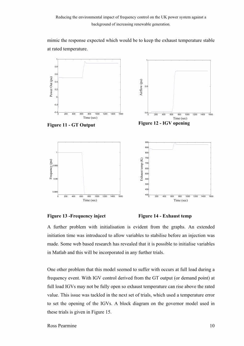
Reducing the environmental impact of frequency control on the UK power system against a
background of increasing renewable generation.
Ross Pearmine 10
mimic the response expected which would be to keep the exhaust temperature stable
at rated temperature.
Figure 11 - GT Output Figure 12 - IGV opening
Figure 13 -Frequency inject Figure 14 - Exhaust temp
A further problem with initialisation is evident from the graphs. An extended
initiation time was introduced to allow variables to stabilise before an injection was
made. Some web based research has revealed that it is possible to initialise variables
in Matlab and this will be incorporated in any further trials.
One other problem that this model seemed to suffer with occurs at full load during a
frequency event. With IGV control derived from the GT output (or demand point) at
full load IGVs may not be fully open so exhaust temperature can rise above the rated
value. This issue was tackled in the next set of trials, which used a temperature error
to set the opening of the IGVs. A block diagram on the governor model used in
these trials is given in Figure 15.
0 200 400 600 800 1000 1200 1400 1600-0.4
-0.2
0
0.2
0.4
0.6
0.8
1
Time (sec)
Po
wer
Out
(pu
)
0 200 400 600 800 1000 1200 1400 16000.6
0.8
1
Time (sec)
Air
flo
w (
pu
)
0 200 400 600 800 1000 1200 1400 1600
0.985
0.99
0.995
1
Time (sec)
Fre
quen
cy (
pu
)
0 200 400 600 800 1000 1200 1400 1600400
450
500
550
600
650
700
750
800
850
900
Time (sec)
Exh
aust
tem
p (
K)
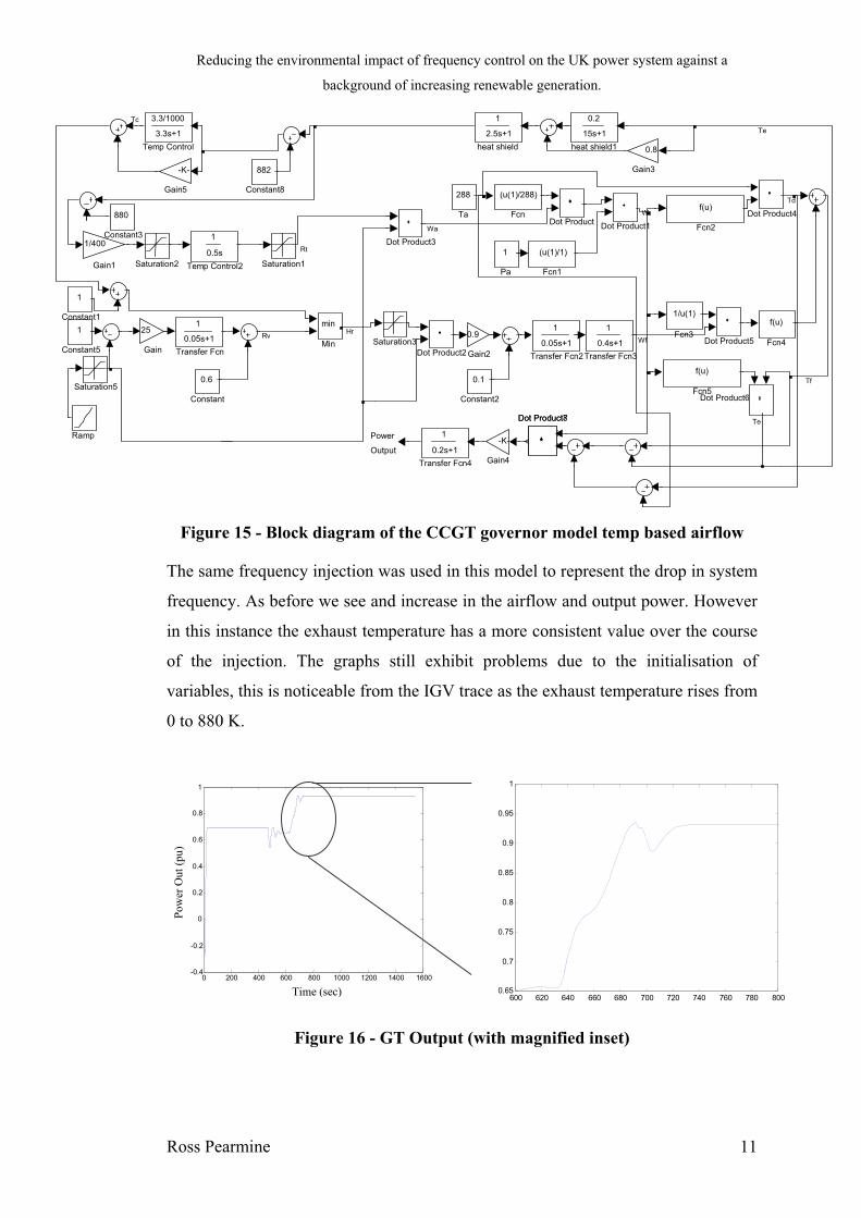
Reducing the environmental impact of frequency control on the UK power system against a
background of increasing renewable generation.
Ross Pearmine 11
Figure 15 - Block diagram of the CCGT governor model temp based airflow
The same frequency injection was used in this model to represent the drop in system
frequency. As before we see and increase in the airflow and output power. However
in this instance the exhaust temperature has a more consistent value over the course
of the injection. The graphs still exhibit problems due to the initialisation of
variables, this is noticeable from the IGV trace as the exhaust temperature rises from
0 to 880 K.
Figure 16 - GT Output (with magnified inset)
0.2
15s+1
heat shield1
1
2.5s+1
heat shield
1
0.2s+1
Transfer Fcn4
1
0.4s+1
Transfer Fcn3
1
0.05s+1
Transfer Fcn2
1
0.05s+1
Transfer Fcn
1
0.5s
Temp Control2
3.3/1000
3.3s+1
Temp Control
288
Ta
Saturation5
Saturation3
Saturation2 Saturation1
Ramp
1
Pa
min
Min
-K-
Gain5
-K-
Gain4
0.8
Gain3
0.9
Gain2
1/400
Gain1
25
Gain
f(u)
Fcn5
f(u)
Fcn4
1/u(1)
Fcn3
f(u)
Fcn2
(u(1)/1)
Fcn1
(u(1)/288)
Fcn
Dot Product8Dot Product7
Dot Product6
Dot Product5
Dot Product4
Dot Product3
Dot Product2
Dot Product1Dot Product
882
Constant8
1
Constant5
880
Constant3
0.1
Constant2
1
Constant1
0.6
Constant
RvHr
Wa
Wf
W
Td
Tf
Te
Te
Rt
Tc
Power
Output
0 200 400 600 800 1000 1200 1400 1600-0.4
-0.2
0
0.2
0.4
0.6
0.8
1
Time (sec)
Po
wer
Out
(pu
)
600 620 640 660 680 700 720 740 760 780 8000.65
0.7
0.75
0.8
0.85
0.9
0.95
1

Reducing the environmental impact of frequency control on the UK power system against a
background of increasing renewable generation.
Ross Pearmine 12
Figure 17 - IGV opening Figure 18 - Exhaust temp
These initial trials offer a degree of coherence with the actual response experienced
on the system in Figure 4. Work will continue to develop this models for use with
the ABB GT26 machine.
0 200 400 600 800 1000 1200 1400 16000
100
200
300
400
500
600
700
800
900
1000
Time (sec)
Exh
aust
tem
p (
K)
0 200 400 600 800 1000 1200 1400 16000.6
0.8
1
Time (sec)
Air
flo
w (
pu
)
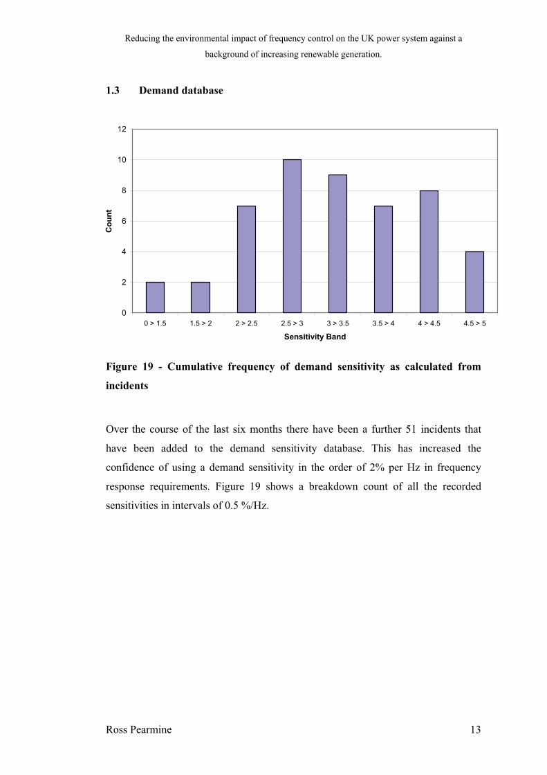
Reducing the environmental impact of frequency control on the UK power system against a
background of increasing renewable generation.
Ross Pearmine 13
1.3 Demand database
Figure 19 - Cumulative frequency of demand sensitivity as calculated from
incidents
Over the course of the last six months there have been a further 51 incidents that
have been added to the demand sensitivity database. This has increased the
confidence of using a demand sensitivity in the order of 2% per Hz in frequency
response requirements. Figure 19 shows a breakdown count of all the recorded
sensitivities in intervals of 0.5 %/Hz.
0
2
4
6
8
10
12
0 > 1.5 1.5 > 2 2 > 2.5 2.5 > 3 3 > 3.5 3.5 > 4 4 > 4.5 4.5 > 5
Sensitivity Band
Co
un
t

Reducing the environmental impact of frequency control on the UK power system against a background of increasing renewable generation.
2.0 Next 6 months
Years 2004 2005 2006
Months
Activity Oct Nov Dec Jan Feb Mar Apr May Jun Jul Aug Sept Oct Nov Dec Jan Feb Mar Apr May Jun Jul Aug Sept Oct Nov Dec
Progress report 2nd Year
viva
6 Month
Report
6 Month
Report
6 Month
Report Final Report
EngD
Conf
Economic
Approaches Energy Materials
Modules /conferences
Wind power module Finance
Validate steam turbine models against individual plant
Develop CCGT model against individual plant
Review existing incidents using validated models
Add Scottish nodes to grid model
Write/Submit paper1
Write/Submit paper2
Review response requirements examining effects of
geographic reserve holding
Review literature on modelling of wind turbines
Build wind farm model
Validate Wind farm model
Review response requirements with integration of wind
model
Translate response requirements into CO2 emissions
Final write up
Corrections/references/prepare for viva
24 M
onth
Rep
ort
Gen
erator an
d L
oad
Beh
avio
ur
R.P
earmin
e
Ro
ss Pearm
ine
1
4

Reducing the environmental impact of frequency control on the UK power system against a
background of increasing renewable generation.
Ross Pearmine 15
Difficulties in developing and implementing of the CCGT governor model have set
back the project by approximately one month. In order to keep to the required
schedule I have increased development time on the CCGT models by one month and
reduced the time devoted to testing against real incidents. I feel this can be achieved
by only testing each model in manufacturer range, and not every generating station.
This halves the required testing and should not effect the results. A have further
reduced the time to implement the Scottish nodes into the network as this can be
achieved through importing the network from other existing packages. However the
databases that are used to retrieve demand and generation will still need to be
reworked.
In the next six months it is hoped that the following can be achieved to the revised
schedule.
Add a response limit to coal fired generation that can be defined by contract
values
Ensure every generator has a simulation from a large frequency drop
Initialise variables in Matlab to allow further trials with CCGT models
Model an actual events in Matlab
Model different types of manufacturer, and implement in Eurostag
Continue to monitor demand sensitivity
Review response requirements examining effects of geographic reserve
holding
Write/Submit paper1
Add Scottish nodes to grid model

Reducing the environmental impact of frequency control on the UK power system against a
background of increasing renewable generation.
Ross Pearmine 16
3.0 Summary
This report explains the current developments in validating coal fired governor
models against real incidents. Work is required to further increase the accuracy of the
models in some cases.
Development of a governor model for CCGT plant has also been started. A suitable
model has been identified for possible use with ABB GT26 plant. Development of
this model is expected for the next six months.
It still holds that the assumed National grid value of 2% seems to be accurate.
Within the next six months it is hoped that a paper will be written to submission to the
IEEE.
4.0 References
[1] Combined Cycle Plants: Models and In-Situ Reliability Tests
Agüero, J.L.; Beroqui, M.; Molina, R.;
Power Engineering Society Summer Meeting, 2001. IEEE
Volume: 3, 15-19 July 2001
Page(s):1788 - 1793
[2] Performance of gas turbine-based plants during frequency drops
Kakimoto, N.; Baba, K.;
Power Systems, IEEE Transactions on
Volume 18, Issue 3, Aug. 2003
Page(s):1110 - 1115
[3] Model Development and Simulation of Transient Behaviour of Heavy Duty
Gast Turbines
Kim, J.H.; Song, T.W.; Kim, T.S.; Ro, S.T.;
Journal of Engineering for Gas Turbines and Power
Reducing the environmental impact of frequency control on the UK power system against a
background of increasing renewable generation.
Ross Pearmine 17
Volume: 123, July 2001
Page(s): 589 – 594
[4] Modeling frequency dependency of gas turbine output
Kunitomi, K.; Kurita, A.; Okamoto, H.; Tada, Y.; Ihara, S.; Pourbeik, P.;
Price, W.W.; Leirbukt, A.B.; Sanchez-Gasca, J.J.;
Power Engineering Society Winter Meeting, 2001. IEEE
Volume 2, 28 Jan.-1 Feb. 2001
Page(s):678 - 683 vol.2
[5] Simplified Mathematical Representations of Heavy-Duty Gas Turbines
Rowen, W.I.;
ASME Paper 83-GT-63; Oct. 1983
[6] Simplified Mathematical Representations of Single Shaft Gas Turbines in
Mechanical Drive Service
Rowen, W.I.;
ASME Paper 92-GT-22; June 1992
[7] Modeling of combined cycle plants in grid simulation studies
Undrill, J.; Garmendia, A.;
Power Engineering Society Winter Meeting, 2001. IEEE
Volume 2, 28 Jan.-1 Feb. 2001
Page(s):657 - 663 vol.2
[8] Dynamic models for combined cycle plants in power system studies
Working group on prime mover and energy supply models for system dynamic
performance studies
Power Systems, IEEE Transactions on
Volume 9, Issue 3, Aug. 1994
Page(s):1698 - 1708

Reducing the environmental impact of frequency control on the UK power system against a
background of increasing renewable generation.
Ross Pearmine i
Six Monthly Progress Report: Sixth Report
Section Title Page
1.0 ... ............................................ Work to Date ......................................................1
1.1................................Coal Fired Generation...............................................1
1.2...... Experiences Validating Coal Fired Governor Models .....................1
1.3........................................ CCGT Plant .......................................................4
1.4.................................. Relevant Literature ...............................................10
2.0 ... ..... Impacts of Governor Models in grid frequency simulations. .............11
3.0 ... ........................................ Demand Database ................................................13
4.0 ... ............................... Targets from previous report.......................................13
5.0 ... ............................................Next 6 months....................................................14
6.0 ... ............................................. Project Plan .....................................................15
6.1...........................................Summary........................................................16
7.0 ... ...............................................References.......................................................16

Reducing the environmental impact of frequency control on the UK power system against a
background of increasing renewable generation.
Ross Pearmine 1
1.0 Work to Date
1.1 Coal Fired Generation
Following work set out in the previous progress report in validating coal fired
generators it was apparent that some machines seemed to be showing a rate limited
response. This response was only apparent during exceptionally large frequency
deviations greater than 0.2Hz in most cases. Due to this circumstance the original
validation trails needed review to ensure that the machines had been validated
against at least two or three large frequency deviations. This would then prove the
nature of the response under governor action.
The test methodology followed was the same as in previous examples with a
frequency input in the governor macro-blocks that could be used to inject the
experienced system frequency during trip events. This injected frequency would
cause the generator to respond as would be expected in the real event allowing a
comparison with recorded values.
Obtaining a realistic governor response is vital in simulating network frequency
during transient disturbances.
1.2 Experiences Validating Coal Fired Governor Models
Analysis of recorded performance data has allowed three distinct groups of governor
model to be identified on the system.
a. Standard droop model
b. Limited droop model
c. Rate limited frequency trip model
Examples of each of these generator responses are shown in Figure 1,Figure 2 and
Figure 4.
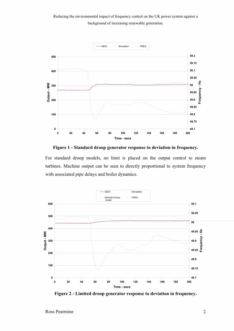
Reducing the environmental impact of frequency control on the UK power system against a
background of increasing renewable generation.
Ross Pearmine 2
Figure 1 - Standard droop generator response to deviation in frequency.
For standard droop models, no limit is placed on the output control to steam
turbines. Machine output can be seen to directly proportional to system frequency
with associated pipe delays and boiler dynamics.
Figure 2 - Limited droop generator response to deviation in frequency.
0
100
200
300
400
500
0 20 40 60 80 100 120 140 160 180 200
Time - secs
Ou
tpu
t -
MW
49.7
49.75
49.8
49.85
49.9
49.95
50
50.05
50.1
50.15
50.2
Fre
qu
en
cy
- H
z
GES1 Simulation FREQ
0
100
200
300
400
500
600
0 20 40 60 80 100 120 140 160 180 200
Time - secs
Ou
tpu
t -
MW
49.7
49.75
49.8
49.85
49.9
49.95
50
50.05
50.1F
req
ue
nc
y -
Hz
GES1 Simulation
Standard droop model
FREQ

Reducing the environmental impact of frequency control on the UK power system against a
background of increasing renewable generation.
Ross Pearmine 3
Limited droop model, in addition to associated pipe delays and boiler dynamics has
a limit imposed on the magnitude of response supplied. The limit is related to
machine loading levels. The chief reasoning behind operating plant in this manner is
to reduce thermal loading in steam pipes and boiler waterwalls. Poor operational
decisions can lead to fatigue cracking such as that shown in Figure 3.
Figure 3 - Fatigue cracks in boiler steam pipes
The output is no longer proportional to system frequency. Comparison with a
simulation of the same unit acting under the standard droop model shows the
increased error in primary response resulting from incorrect use of the model. This
error would have been experienced in early frequency response simulations.
The final governor model in operation on generators is a Rate limited frequency trip
model. This controller is similar to the standard droop model for frequency control
above 49.8Hz. Below this threshold a limited response is tripped allowing a
maximum rate of power increase in the order of 1 MWs-1
.
The chief reasoning behind operating plant in this manner is again to reduce thermal
loading in steam pipes and the boiler. This has very little influence under secondary
response time scales, but a noticeable impact during the primary response interval.
As with the previous model, comparison with simulations acting under the standard
droop model show the increased error in primary response resulting from incorrect

Reducing the environmental impact of frequency control on the UK power system against a
background of increasing renewable generation.
Ross Pearmine 4
model selection. Again, this error would have been experienced in early frequency
response simulations.
Figure 4 - Rate limited frequency trip generator response to deviation in
frequency.
1.3 CCGT Plant
A simple governor model developed in a Matlab environment detailed in a previous
report had shown a potential for representation of CCGT response during frequency
drops. To provide a governor controller that can be used in system simulation
studies the model required coding from Matlab into Eurostag macro block format.
The task of providing a Eurostag macro block was not as straightforward as had
been originally thought. Problems occurred in initialising variables, and getting
consistency in simulation variables. Valuable experience was gained on how to
implement the macro blocks, which will be useful in constructing future CCGT
models for different manufacturers.
0
100
200
300
400
500
0 20 40 60 80 100 120 140 160 180 200
Time - secs
Ou
tpu
t -
MW
49.4
49.5
49.6
49.7
49.8
49.9
50
Fre
qu
en
cy
- H
z
GES2 Standard droop model
Simulation FREQ

Reducing the environmental impact of frequency control on the UK power system against a
background of increasing renewable generation.
Ross Pearmine 5
A block diagram of the implemented model is given in Figure 5a, b and c, with
corresponding variables in Table 1 and Table 2.
%FPIGV -0.1 0.6
0.7 0.6
0.765 0.8
1. 1.
1.1 1.
KRAD 0.1
KTEMP 3.3
MUCOMP 0.91
MUTURB 0.67
RC 0.2
TR 898.
TRAD 15.
TTEMP 250.
Table 1 - GT26 gas turbine governor variables
%FHRSG 0 0
0.5 0.5
0.8 0.8
1. 1.
TB 200
TS 5
Table 2 - GT26 heat recover steam generator governor variables

Reducing the environmental impact of frequency control on the UK power system against a
background of increasing renewable generation.
Ross Pearmine 6
Figure 5a - Block diagram of the GT26 gas turbine governor macro block
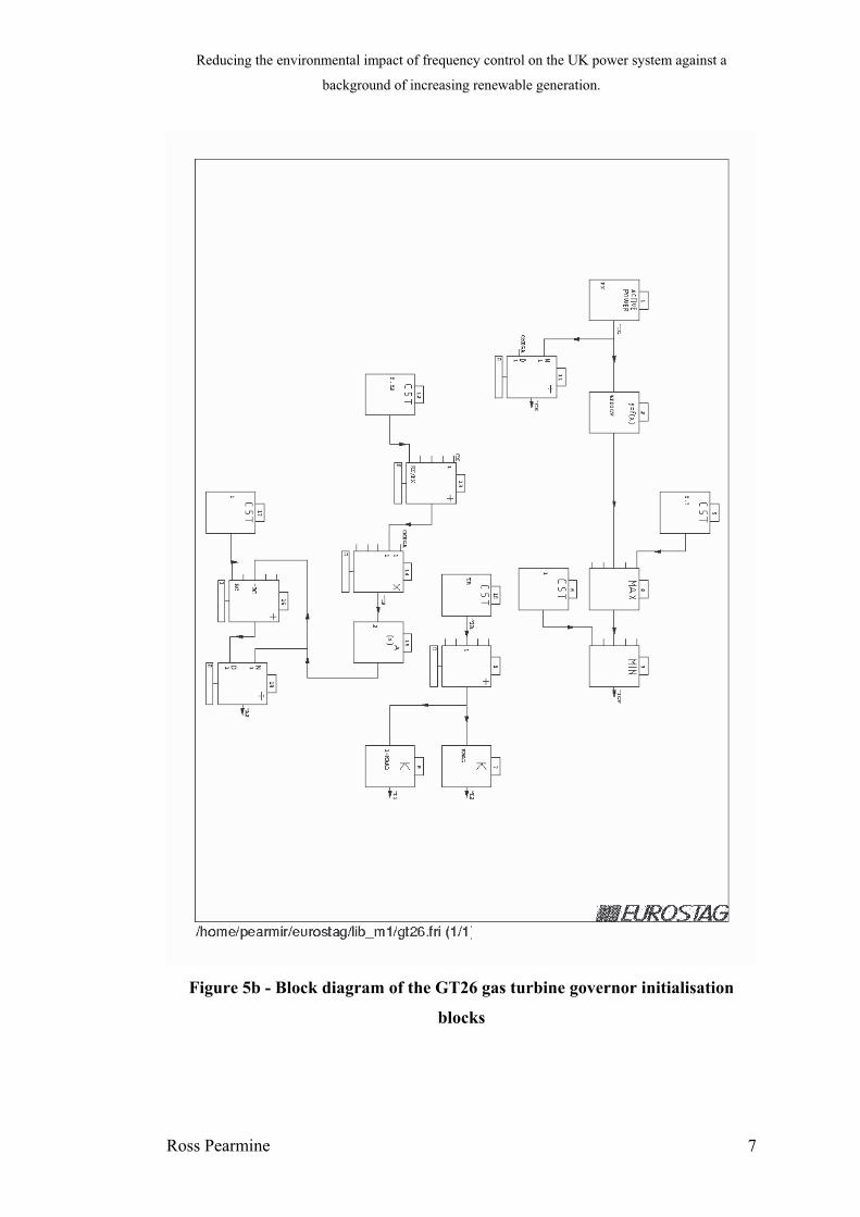
Reducing the environmental impact of frequency control on the UK power system against a
background of increasing renewable generation.
Ross Pearmine 7
Figure 5b - Block diagram of the GT26 gas turbine governor initialisation
blocks
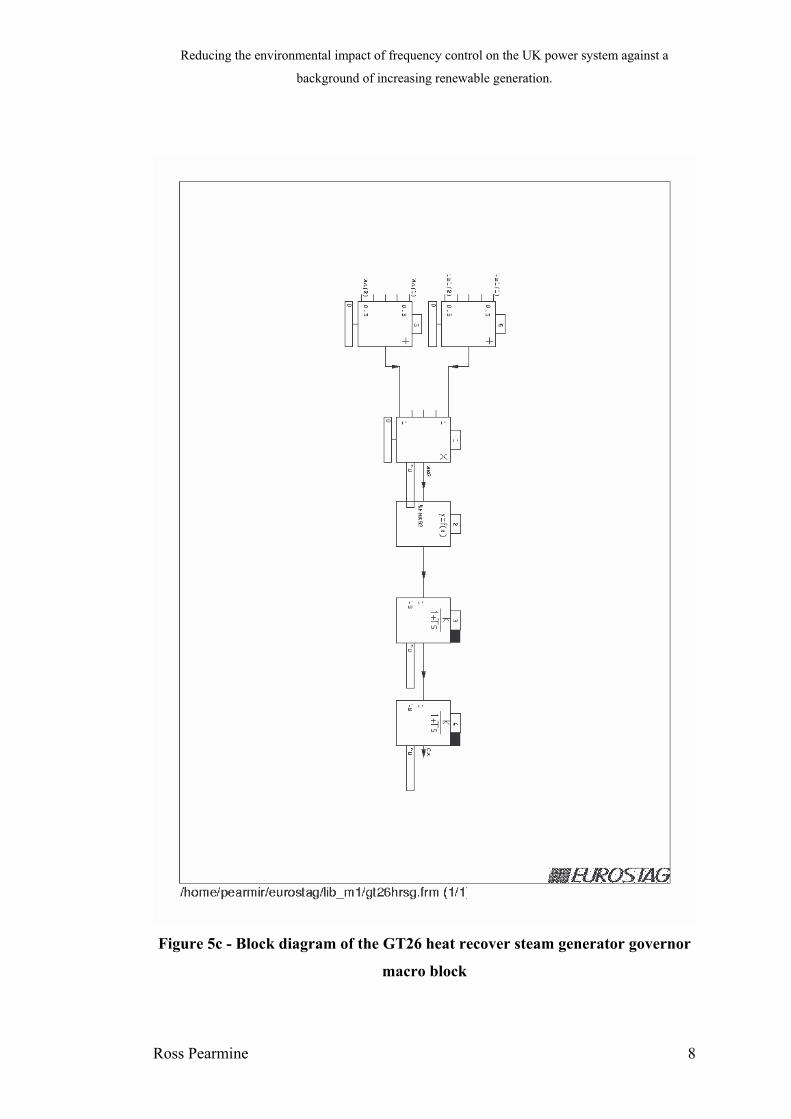
Reducing the environmental impact of frequency control on the UK power system against a
background of increasing renewable generation.
Ross Pearmine 8
Figure 5c - Block diagram of the GT26 heat recover steam generator governor
macro block

Reducing the environmental impact of frequency control on the UK power system against a
background of increasing renewable generation.
Ross Pearmine 9
Simulations of a frequency event where conducted with the model to validate its
response. Figure 6 shows the results of a simulation trial conducted in Eurostag with
the updated governor model for GT26 turbines. These models give an improvement
on response in the initial stages of the simulation compared to the generic models.
However, it is clear that further improvements can be made to increase the accuracy.
Figure 6 - Simulated GT26 response to an actual -0.6 Hz frequency drop.
In the above example, GT1 does not reach the peak output experienced on the actual
unit. This is due to the use of load controllers on the plant. Load controllers monitor
the response of the whole plant (two gas turbines and steam turbine) to ensure that
the required collective response of the power station is met. In this case the driving
signal to both gas turbines would have been greater than the normal 4% droop on
other machines because of the slow response of the steam unit.
A simple macro block can be introduced to provide the function of a load controller.

Reducing the environmental impact of frequency control on the UK power system against a
background of increasing renewable generation.
Ross Pearmine 10
This will be developed and tested against further incidents that led to a considerable
deviation in frequency.
1.4 Relevant Literature
A number of papers have been published recently from research conducted on the
Irish electricity grid. This research has developed with what seems the same
objective set out by National Grid in this project. References to earlier work
investigating the load frequency characteristic of the Irish Grid [2] had been made in
the transfer viva [1].
Further studies [3][4][5] have progressed with particular attention to frequency
response of combined-cycle plant which has been mentioned in section 1.3 of this
report. A number of possible problems arise in the methodology adopted by
O’Malley. The frequency studies have been conducted using a single bus system to
represent the entire Irish grid. The authors are aware that this technique assumes all
grid frequency is uniform across the grid. However, studies have shown that this is
not the case. Whilst monitoring generator data from the UK grid it is evident the
local grid frequencies rarely deviated from each other within a band of 0.1Hz.
In conjunction with homogeneous grid frequency there is also a more significant
impact in that the node voltages must also be uniform. This assumption has a greater
bearing on the simulations as in many cases the voltages across the network will
vary according to node impedances. These impedances are very different for each of
the substations on the grid, due to varied components, substation configurations and
connections to distribution networks. Generators also act to control these voltages
through AVRs which have an impact on the generator dynamic performance.
The second inaccuracy from the view point of the UK grid is the representation of
all gas turbines has been made through Rowen’s Models [6][7]. It has been shown
through this research that the operating characteristics of ABB and GE turbines are
critically different (not considering Siemens or Mitsubishi plants). As such the final
simulated grid frequency is heavily dependant on the chosen model to represent each

Reducing the environmental impact of frequency control on the UK power system against a
background of increasing renewable generation.
Ross Pearmine 11
turbine. Without looking at the composition of grid connected CCGTs in Ireland it is
impossible to say if the published results are affected by this oversight.
The latest research has been conducted in the impacts of increasing proportions of
wind turbines on the system [8]. The paper has considered two cases; case one with
all variable speed DFIG units, case two all units fixed speed units. The cases
represent those units that will not contribute to the inertial response of the system
and those that will respectively. The results show an influence on the initial rate of
change of frequency as to be expected and also the minimum frequency in both
cases. The severity of the disturbance is far greater with all wind turbines being
DFIG units.
This results was to be expected in the case of the UK system, however the different
makeup of the UK super grid will have an impact on the severity of the disturbance.
With the UK grid being much larger in size it requires a large in-feed loss to provide
deviations anywhere near those seen on the Irish grid. It is this difference and the
use of a 630-bus system model which provides a further contribution to knowledge
seen by this project.
2.0 Impacts of Governor Models in grid frequency simulations.
With alterations made to the governor models of thermal plant in section 1.2, and a
more accurate representation of GT26 turbines from section 1.3, a frequency
incident was revisited. The event chosen was initially studied in the transfer viva and
remains one of the largest frequency transients experienced by the National Grid
system. For the simulation the network configuration files remained untouched and
only the generator data file was altered to include the new validated governor macro
blocks. Non-GT26 CCGT gas turbine governor models were replaced with the GE
based GASTURB model included in the Eurostag package.
Figure 7and Figure 8 show the output simulations of the event together with the
actual recorded system values. The significant improvement in modelling of the

Reducing the environmental impact of frequency control on the UK power system against a
background of increasing renewable generation.
Ross Pearmine 12
generator responses is evident when comparing the charts to the early investigation
[1]. Closer inspection of the frequency trace shows good match with the grid
frequency in primary time scales. There is a noticeable difference at the secondary
time scales of around 0.15Hz. This may be in part still due to the need to validate the
CCGT plant and review the models for non-GT26 turbines.
Figure 7 - Simulation of 1260 MW generation loss 26/05/03; Frequency
Figure 8 - Simulation of 1260 MW loss 26/05/03; Responsive Generation
49.3
49.4
49.5
49.6
49.7
49.8
49.9
50
0 10 20 30 40 50 60
Time - sceonds
Fre
qu
en
cy
- H
z
Simulated Frequency Grid Frequency
8000
8200
8400
8600
8800
9000
9200
9400
0 10 20 30 40 50 60
Time - seconds
Cu
mu
lati
ve
Ou
tpu
t -
MW
Simulated Responsive Generators Grid Cumulative Response

Reducing the environmental impact of frequency control on the UK power system against a
background of increasing renewable generation.
Ross Pearmine 13
However, the initial results showing generator response in Figure 8 look promising,
and are certainly an improvement.
3.0 Demand database
Over the course of the last six months the number of recorded frequency incidents
rose to 81. This has allowed a journal paper to be submitted to the IEE Proceedings
on Generation, Transmission & Distribution. Through statistical analysis of the
recorded demand sensitivity it has been possible to derive a probability distribution
for the values. This enables a minimum expected load response to be identified for
network security.
The paper provides further support that the current load frequency sensitivity factor
of 2 %MW/Hz is justified. It suggests that the value may even be extended to a
value of 2.5 %MW/Hz. Therefore, this value can be substituted into the calculations
for response requirements on the electricity grid in Great Britain.
4.0 Targets from previous report
A number of milestones where met from the previous report including:
Monitoring of demand sensitivity
Ensure every generator has a simulation from a large frequency drop
Add a response limit to coal fired generation that can be defined by contract
values
Write/Submit paper1
Add Scottish nodes to grid model
However, the following tasks where not achieved:
Model actual events in Matlab

Reducing the environmental impact of frequency control on the UK power system against a
background of increasing renewable generation.
Ross Pearmine 14
Model different types of manufacturer, and implement in Eurostag
Review response requirements examining effects of geographic reserve holding
To ensure that these tasks are completed where necessary and that the project
remains on schedule a review of the project plan has been conducted.
5.0 Next 6 months
Difficulties in validating and implementing of the coal fired governor model
together with unrealistic estimates of the time spent writing up course work for
EngD modules have set back the project substantially. In order to keep to the
required schedule I have removed the task of reviewing the response requirements
examining effects of geographic reserve holding. If time allows at the later stages of
the project this task may be reintroduced into the project plan.
I feel this is justified, as the task does not have a great bearing on the objectives of
the project. It was originally included as an investigation piece to evaluate if
geographic response holding should be a consideration for future policy. With only
one further module to attend in the final year a solid twelve-month window exists to
complete research. By restructuring the remaining tasks completion of all research in
the allotted time scales is reasonable and attainable.
In the next six months it is hoped that the following can be achieved to the revised
schedule.
Validation of CCGT models in Eurostag
Model actual frequency events in Eurostag
Obtain data to validate a suitable model for representing wind turbines in
simulations studies
Start review of response requirements

Reducing the environmental impact of frequency control on the UK power system against a background of increasing renewable generation.
6.0 Project Plan
Years 2004 2005 2006
Months
Activity Oct Nov Dec Jan Feb Mar Apr May Jun Jul Aug Sept Oct Nov Dec Jan Feb Mar Apr May Jun Jul Aug Sept Oct Nov Dec
Progress report 2nd Year
viva
6 Month
Report
6 Month
Report
6 Month
Report Final Report
EngD
Conf
Economic
Approaches Energy Materials
Commu
nication
Modules /conferences
Wind power module Finance
Validate steam turbine models against individual plant
Develop CCGT model against individual plant
Review existing incidents using validated models
Add Scottish nodes to grid model
Write/Submit paper1
Write/Submit paper2
Review literature on modelling of wind turbines
Build wind farm model
Validate Wind farm model
Review response requirements with integration of wind
model
Translate response requirements into CO2 emissions
Final write up
Corrections/references/prepare for viva
24 M
onth
Rep
ort
Gen
erator an
d L
oad
Beh
avio
ur
R.P
earmin
e
Ro
ss Pearm
ine
1
5

Reducing the environmental impact of frequency control on the UK power system against a
background of increasing renewable generation.
Ross Pearmine 16
6.1 Summary
This report explains the current developments in validating coal fired governor models
against real incidents. Work is required to further increase the accuracy of the models in
some cases.
Development of a governor model for CCGT plant has also been started. A suitable
model has been identified for use with ABB GT26 plant. Development of this model will
continue for the next month, with validation trails against all grid connected units.
Further validation of other CCGT units on the system will also be conducted.
It still holds that the assumed National grid value of 2% seems to be accurate.
Within the next six months it is hoped that a second paper will be written and submitted
to the IEEE.
7.0 References
[1] Reducing the environmental impact of frequency control on the UK power
system against a background of increasing renewable generation.
Pearmine, R.S.;
Transfer Viva, Brunel University; Oct 2004
[2] Identification and validation of dynamic global load model parameters for
use in power system frequency simulation
O’Sullivan, J. W.; O’Malley, M. J.;
Power Systems, IEEE Transaction on,
Volume: 11, Issue: 2, May 1996
[3] Frequency Control in Competitive Electricity Market Dispatch
Doherty, R.; Lalor, G.; O'Malley, M.;
Power Systems, IEEE Transactions on
Volume 20, Issue 3, Aug. 2005

Reducing the environmental impact of frequency control on the UK power system against a
background of increasing renewable generation.
Ross Pearmine 17
[4] The Impact of Combined-Cycle Gas Turbine Short-Term Dynamics on
Frequency Control
Lalor, G.; Ritchie, J.; Flynn, D.; O'Malley, M.J.;
Power Systems, IEEE Transactions on
Volume 20, Issue 3, Aug. 2005
[5] Frequency control on an island power system with increasing proportions
of combined cycle gas turbines
Lalor, G.; O'Malley, M.;
Power Tech Conference Proceedings, 2003 IEEE Bologna
Volume 4, 23-26 June 2003
[6] Simplified Mathematical Representations of Heavy-Duty Gas Turbines
Rowen, W.I.;
ASME Paper 83-GT-63; Oct. 1983
[7] Simplified Mathematical Representations of Single Shaft Gas Turbines in
Mechanical Drive Service
Rowen, W.I.;
ASME Paper 92-GT-22; June 1992
[8] Dynamic frequency control with increasing wind generation
Lalor, G.; Ritchie, J.; Rourke, S.; Flynn, D.; O'Malley, M.J.;
Power Engineering Society General Meeting, 2004. IEEE
6-10 June 2004

Reducing the environmental impact of frequency control on the UK power system against a
background of increasing renewable generation.
Ross Pearmine i
Six Monthly Progress Report: Seventh Report
Section Title Page
1.0 ... ............................................ Work to Date ......................................................1
1.1 CCGT Plant validation ..............................................1
1.2........................ Full grid frequency simulations .......................................4
1.3.......................Review of response requirements......................................7
2.0 ... ...................................Demand response paper............................................11
3.0 ... ............................... Targets from previous report.......................................11
4.0 ... ............................................Next 6 months....................................................11
5.0 ... ............................................. Project Plan .....................................................13
6.0 ... ................................................Summary........................................................14
7.0 ... ...............................................References.......................................................14

Reducing the environmental impact of frequency control on the UK power system against a
background of increasing renewable generation.
Ross Pearmine 1
1.0 Work to Date
1.1 CCGT Plant validation
The developed model for CCGT plant was validated against tests carried out on
existing units or historic data. These tests form a basis to demonstrate compliance
with the Grid Code and are conducted on all grid-connected and large embedded
plant. As in previous reports the frequency injection signal is provided to the
governor to simulate the grid frequency during a real transient. Various injection
shapes are tested; the one chosen to validate against in this example is the 0.8Hz
ramp over 10 seconds, returning to 0.5 Hz at a load set point of 60 %. Power output,
inlet guide vane position, exhaust temperature and fuel valve positions are
monitored during the test at sampling intervals of 0.1 seconds. As for the original
tests the unit under simulation is synchronised to the full network model as was
experienced on the day of tests. The response of a simulation is shown in Figure 1
against compliance test results.
Figure 1 - Validation of a Siemens V94.3A gas turbine governor model at 60%
load.
0.0%
10.0%
20.0%
30.0%
40.0%
50.0%
60.0%
70.0%
80.0%
90.0%
100.0%
0 20 40 60 80 100 120 140
Time (Secs)
Va
lve
Po
sit
ion
(%
)
Fuel Valve WF
0
10
20
30
40
50
60
70
80
90
0 20 40 60 80 100 120 140
Time (Secs)
IGV
Po
sit
ion
(%
)
500
510
520
530
540
550
560
570
580
EG
T (
De
g C
)
IGV % WA Exhaust temp. T
100
120
140
160
180
200
220
0 20 40 60 80 100 120 140
Time (Secs)
Ac
tiv
e P
ow
er
(MW
)
-0.90
-0.80
-0.70
-0.60
-0.50
-0.40
-0.30
-0.20
-0.10
0.00
0.10
Fre
qu
en
cy
(H
z)
GT Power Pgt Finj Finj
150
155
160
165
170
175
180
0 20 40 60 80 100 120 140
Time (Secs)
Ac
tiv
e P
ow
er
(MW
)
ST Power Pst

Reducing the environmental impact of frequency control on the UK power system against a
background of increasing renewable generation.
Ross Pearmine 2
The fuel valve position signal from tests shows an opening from 60 to 73% as
frequency is injected, this is met by a rise from 60 to 87% in the model. However,
despite this difference the overall power output of the model remains within a tight
tolerance of actual unit, suggesting a supplementary fuel valve that was not
monitored during tests. The test frequency injection is a summation of grid
frequency and injection signal hence the signal is not as crisp as that seen in the
simulation due to minor fluctuations in the grid frequency. Figure 2 shows the
change in power for the same CCGT unit and model at a slightly higher loading
point.
Figure 2 - Power output from Siemens V94.3A gas turbine governor model at
73% load.
Marginal differences between the simulation of inlet guide vane position and
exhaust temperature from the test results bring attention to insufficient modelling of
temperature limit controls. This is also noticeable in the simulated power output
curve as it reaches peak output, which is not limited to the same level as the actual
unit. Output power, as simulated by the model, provides a close match to the
compliance test in the initial 30 seconds of the trip. This time scale is critical for
establishing response levels that curtail the drop in frequency. Response on
secondary time scales whilst important to restore system operation back to normality
does not critically influence the risks of demand disconnection provided it is
0
50
100
150
200
250
0 20 40 60 80 100 120 140
Time (Secs)
Ac
tiv
e P
ow
er
(MW
)
-0.90
-0.80
-0.70
-0.60
-0.50
-0.40
-0.30
-0.20
-0.10
0.00
0.10
Fre
qu
en
cy
(H
z)
GT Power Pgt Finj Finj

Reducing the environmental impact of frequency control on the UK power system against a
background of increasing renewable generation.
Ross Pearmine 3
sustained from primary levels. Whilst these results show a marked improvement in
comparison with the results obtained from standard models there remains an
opportunity to improve the model.
Instances where actual historic events can be used to validate models offer the
benefit of a real frequency change. However, these events do not provide the
opportunity to analyse data on exhaust temperature and airflow simulated by the
model. Figure 3 shows a simulation of a historic event against the experienced
values.
Figure 3 - Simulation of a frequency drop on an ABB GT26 unit
With accurate governor models of Oil, Coal and CCGT units established the project
can now progress to running full scale network simulations. The development of a
CCGT model and tuning of the generators provides the bulk of the work carried out
to date. The models and data collected are unique from all the papers reviewed from
literature sources. Considering this information a second draft journal paper has
been produced for internal review based on these findings. It is hoped to submit this
paper to the to Electric Power Systems Research journal by the end of March.
0
50
100
150
200
250
300
0 20 40 60 80 100 120 140 160 180 200
Time - secs
Ou
tpu
t -
MW
49.6
49.65
49.7
49.75
49.8
49.85
49.9
49.95
50
50.05
50.1
Fre
qu
en
cy
- H
z
GES1 GES2 GES3 SIM G1 SIM G2 SIM S1 FREQ

Reducing the environmental impact of frequency control on the UK power system against a
background of increasing renewable generation.
Ross Pearmine 4
1.2 Full grid frequency simulations
With a complete library of governor macro blocks the possibility exists to compare
the full network response of the simulation model to actual events. Precise
reproduction of the transient frequency response in the simulations will highlight the
accuracy of the complete model following the developments of the individual
generator governors.
Problems obtaining operational data from the Scottish networks and convergence of
load flows have meant that a reversion back to a lumped model of Scottish
generation and demand was necessary. Building on the simulation carried out in the
last report the event from 26 May 2003 was revisited with the full model, Figure 4.
Increased accuracy has been obtained in both frequency and generation traces.
A second event from 21 January 2006, following the progressive loss of a CCGT
unit totalling 790MW was also simulated, Figure 5. The traces show a very close
match to the experienced event. The load response was increased from 2%/Hz to
4%/Hz inline with calculations from the actual event.
A third event from 2nd
December 2005 simulates the response during a 1GW bipole
trip of the Anglo-French interconnector. During this simulation the lumped Scottish
response is somewhat sluggish compared to the actual event, it is this that is the
main cause of the difference in experienced and simulated grid frequency. Again the
load response was increased from 2%/Hz to 3.7%/Hz inline with the actual event.
Also of note is the fact that the frequency does not recover from 49.7Hz due to
increasing demands at that time.
These three events demonstrate the accuracy of the post event modelling techniques
employed to simulate grid frequency. Now that a high confidence is established in
the model a review of the response holding levels can begin.

Figure 4 - Network response and simulation to a 1.26GW loss 26/05/03
Red
ucin
g th
e env
iron
men
tal imp
act of freq
uen
cy co
ntro
l on
the U
K p
ow
er system
again
st a
back
gro
un
d o
f increasin
g ren
ewab
le gen
eration.
Ro
ss Pearm
ine
5
0.0
100.0
200.0
300.0
400.0
500.0
600.0
700.0
800.0
Resp
on
se, M
WSimulated Response Actual response
49.3
49.4
49.5
49.6
49.7
49.8
49.9
50
0 10 20 30 40 50 60
Time, s
Fre
qu
en
cy, H
z
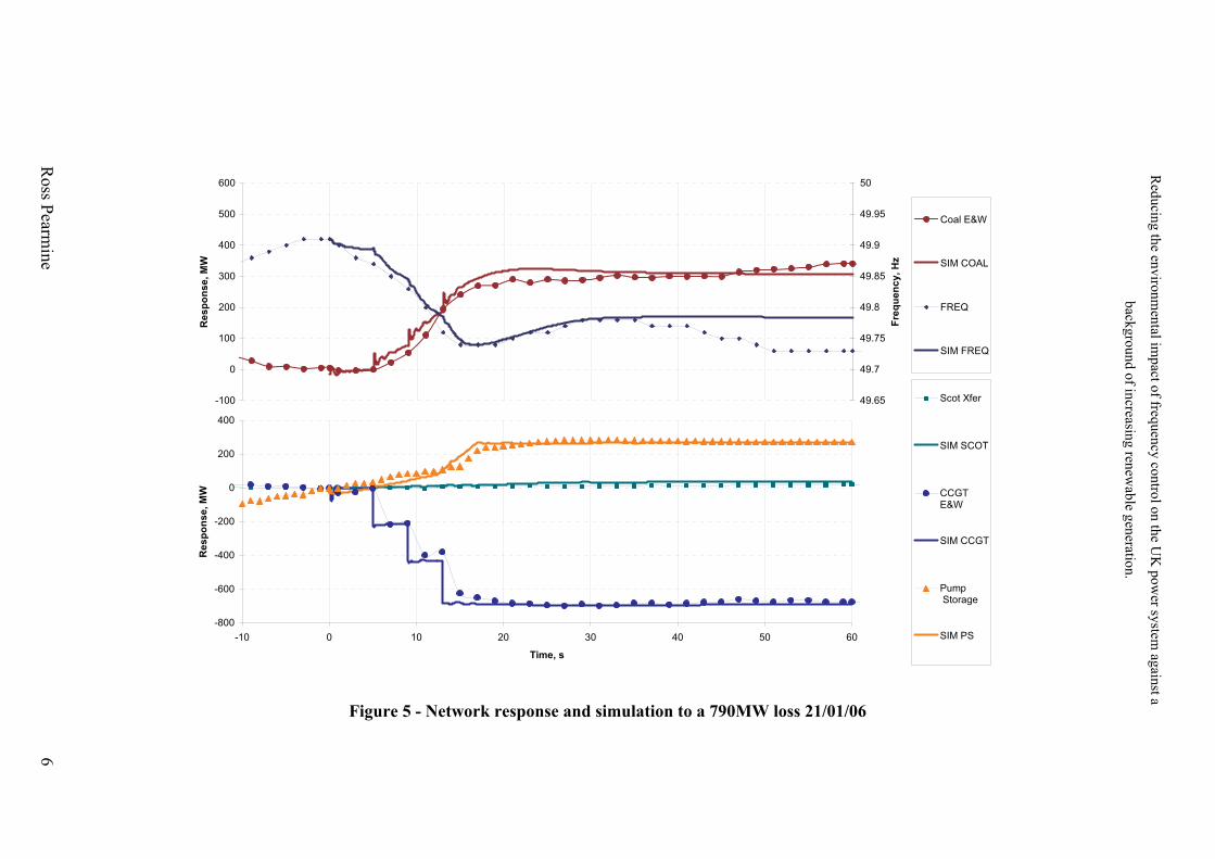
-800
-600
-400
-200
0
200
400
-10 0 10 20 30 40 50 60
Time, s
Re
sp
on
se
, M
W
Scot Xfer
SIM SCOT
CCGTE&W
SIM CCGT
Pump Storage
SIM PS
-100
0
100
200
300
400
500
600
Re
sp
on
se
, M
W
49.65
49.7
49.75
49.8
49.85
49.9
49.95
50
Fre
qu
en
cy
, H
z
Coal E&W
SIM COAL
FREQ
SIM FREQ
Figure 5 - Network response and simulation to a 790MW loss 21/01/06
Red
ucin
g th
e env
iron
men
tal imp
act of freq
uen
cy co
ntro
l on
the U
K p
ow
er system
again
st a
back
gro
un
d o
f increasin
g ren
ewab
le gen
eration.
Ro
ss Pearm
ine
6
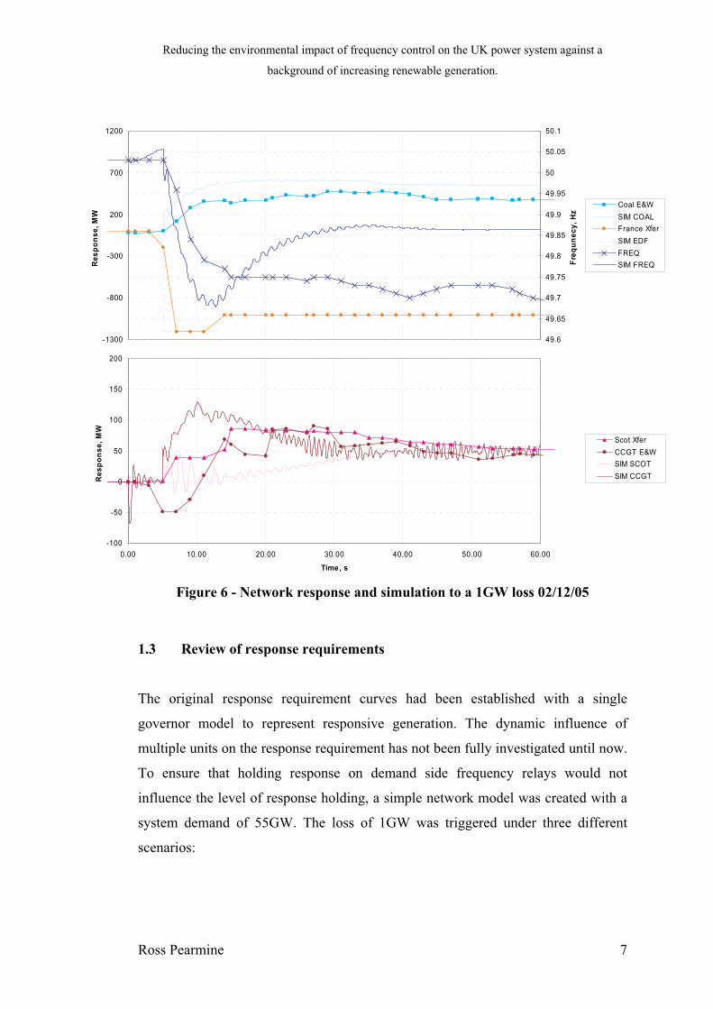
Reducing the environmental impact of frequency control on the UK power system against a
background of increasing renewable generation.
Ross Pearmine 7
-1300
-800
-300
200
700
1200
Re
sp
on
se
, M
W
49.6
49.65
49.7
49.75
49.8
49.85
49.9
49.95
50
50.05
50.1
Fre
qu
ne
cy
, H
z
Coal E&W
SIM COAL
France Xfer
SIM EDF
FREQ
SIM FREQ
-100
-50
0
50
100
150
200
0.00 10.00 20.00 30.00 40.00 50.00 60.00
Time, s
Re
sp
on
se
, M
W
Scot Xfer
CCGT E&W
SIM SCOT
SIM CCGT
Figure 6 - Network response and simulation to a 1GW loss 02/12/05
1.3 Review of response requirements
The original response requirement curves had been established with a single
governor model to represent responsive generation. The dynamic influence of
multiple units on the response requirement has not been fully investigated until now.
To ensure that holding response on demand side frequency relays would not
influence the level of response holding, a simple network model was created with a
system demand of 55GW. The loss of 1GW was triggered under three different
scenarios:

Reducing the environmental impact of frequency control on the UK power system against a
background of increasing renewable generation.
Ross Pearmine 8
Response on Coal Units all with the same governor model + 200MW of demand
side management (50% triggered at 49.7Hz, and a further 50% triggered at
49.65Hz)
Response on Coal Units all with the same governor model
Response on Coal Units each with specific governor models + 200MW of
demand side management
These scenarios would identify differences in response holding levels required to
contain the drop in frequency. As the frequency limit under a 1 GW loss is a
deviation of -0.5Hz, responsive plant output was adjusted and displaced until
frequency fell to 49.5Hz. Figure 7 shows the frequency and cumulative change in
response supplied in each of the three scenarios. The frequency minimum was not
at the same time for each of the transients, as expect. Due to the difference in
dynamic response each frequency trace is unique, however, the traces show that the
level of primary and secondary response under each scenario is similar. In fact,
further analysis of the three scenarios reveals no significant difference in the levels
of response holding at these points.
Figure 7 - Response required to contain a 1GW loss under three test scenarios
0
100
200
300
400
500
600
Coal all 1 Type &
200MW Shedding
No Shedding
Coal + Shedding
49.4
49.5
49.6
49.7
49.8
49.9
50
0 10 20 30 40 50 60 70 80 90 100
Time, s
Fre
que
nc
y, H
zR
esp
onse
, M
W

Reducing the environmental impact of frequency control on the UK power system against a
background of increasing renewable generation.
Ross Pearmine 9
The conclusion from these studies is that the inclusion of demand management in
response trails should have no untoward effect on the net response holding
requirement. These results also highlight the similarities in response levels
calculated from using machines with varying dynamic responses and simulations
when machines have the same dynamic response.
The system quality and security of supply document [1] defines the limits of
frequency that must be sustained during system operation. These limits define a
maximum permissible deviation of -0.8Hz from nominal during abnormal system
incidents. Here abnormal is defined as a generator loss of over 1GW. A second
clause to this limit requires that the system frequency must return to 49.5 Hz before
a minute after the event. In early response trails on abnormal losses the simulation
package was used to define the primary response levels to a deviation reaching
49.2Hz. However, this technique does not necessarily comply with the second part
of the SQSS constraint. Secondary response levels are established through Equation
1.
maxsec,..1 FDRiskR GBSEC
Equation 1
Where;
RSEC = Secondary response holding level
= Error margin
Risk = Largest infeed loss
= Frequency sensitivity to demand
DGB = National Demand
Fsec,max = Maximum permissible deviation under secondary response
timescales
This equation will determine the magnitude of the resulting frequency but imposes
no relation to the time at which this frequency will be attained. Consequently this
may allude to a primary response level which is less than the required power to
prevent a breach of legislated limits.

Reducing the environmental impact of frequency control on the UK power system against a
background of increasing renewable generation.
Ross Pearmine 10
Trials with the full network model at a system demand of 50GW support this
conclusion. Figure 8 shows the simulations conducted at a 50GW national demand
for both the SQSS requirement and the traditional 0.8Hz deviation. An approximate
mismatch of 100MW can be seen in the two situations, with the traditional method
conservative on its result. The current (and Pre-BETTA) response holding levels are
also shown on the figure, they follow the same pattern as the simulations to 0.8Hz.
Figure 8 - Primary response requirements at a 50GW national demand
It is unlikely that the control room would have put the system in any jeopardy by
operating to these levels. By the nature of the response contracts, balancing units can
supply either primary response only or combined primary and secondary response.
To meet the desired levels of response holding the secondary contracts cannot be
acquired as individual ancillary services. In this situation over commitment of
primary response would be more than likely as the secondary requirement is the
driving factor. If the contracting arrangement were ever change to allow a secondary
response market this situation would become more precarious.
Results under secondary time scales have show that calculating the secondary
response requirement using Equation 1 is still acceptable. Further trials are planned
0
100
200
300
400
500
600
700
600 700 800 900 1000 1100 1200 1300 1400
Infeed Risk
Resp
on
se H
old
ing
Holding to
SQSS
Holding to -0.8
Hz deviation
Pre-BETTA
levels
Current levels
Reducing the environmental impact of frequency control on the UK power system against a
background of increasing renewable generation.
Ross Pearmine 11
to establish a set of requirement curves at national demand levels of between 20 and
65GW at 5GW intervals.
2.0 Demand response paper
A paper entitled "Identification of a Load Frequency Characteristic for allocation of
spinning reserves on the UK Electricity Grid" was submitted to the IEE Proceedings
Generation, Transmission and Distribution on the 13th
of September 2005.
Following the submission some major alterations to the paper ensued and a second
revision was submitted 9th
January 2006, the paper was finally accepted for
publication on 11th
Febuary 2006.
3.0 Targets from previous report
A number of milestones where met from the previous report including:
Validation of CCGT models in Eurostag
Model actual frequency events in Eurostag
Start review of response requirements
However, the following tasks where not achieved:
Obtain data to validate a suitable model for representing wind turbines in
simulations studies
Several sources in the UK have been approached to provide data of turbine transient
response during frequency dips. All avenues of investigation have declined
providing information on either technical or commercial grounds. However, if
periods of frequency drops can be identified the data may be soured from the Danish
grid to at least provide some degree of validation.
4.0 Next 6 months

Reducing the environmental impact of frequency control on the UK power system against a
background of increasing renewable generation.
Ross Pearmine 12
Following the work plan submitted in the last six monthly report the project is a
month behind previous expectations, however, a deadline for completion in October
is still realistic. With no further modules expected, and only a conference paper to
write, concentration on simulations can be intensified. Minor adjustments have been
made to the initial task timing in the schedule (see section 6.0) in order to recover
the month lost.
In the next six months it is hoped that the following can be achieved to the revised
schedule.
Implementation and Validation of a wind turbine model in Eurostag
Conclude review of response requirements
Complete response requirements adding a degree of wind power
Conduct sensitivity analysis
Write final thesis
The possibility may also exist to conduct some live system tests with the update
response requirement curves. This would of course lend further credibility to the
work carried out this far on the developed system response model.

5.0 Project Plan
Years 2006
Months
Activity Jan Feb Mar Apr May Jun Jul Aug Sept Oct Nov
Progress report 6 Month Report Final Report
EngD
Conference Modules /conferences
Write/Submit paper2
Write paper for EngD conference
Review existing response requirements
Review literature on modelling of wind turbines
Build wind farm model
Validate Wind farm model
Review response requirements with integration of wind
model
Translate response requirements into CO2 emissions
Final write up
Corrections/references/prepare for viva
Red
ucin
g th
e env
iron
men
tal imp
act of freq
uen
cy co
ntro
l on
the U
K p
ow
er system
again
st a
back
gro
un
d o
f increasin
g ren
ewab
le gen
eration.
Ro
ss Pearm
ine
1
3

Reducing the environmental impact of frequency control on the UK power system against a
background of increasing renewable generation.
Ross Pearmine 14
6.0 Summary
Validation trials have been conducted on a number of combined cycle gas turbines using
both compliance tests and historic events. These tests have been successful in mimicking
the dynamic nature of the plants. This data has provided the possibility of writing a
second paper which it is hoped will be available to submit to the EPRS by the end of
March.
A set of three full network simulations has increased confidence in the response model
adopted. In light of these developments initial simulations have begun to identify a
response requirement. Trials conducted at a system demand of 50GW have revealed
shortcomings in the existing requirement curves. Future work to establish curves for the
remaining demand points has been set against project timescales. Implementation of a
wind turbine model in Eurostag is required to complete the analysis of future response
holding requirements with increased renewables.
The next report will consist of the project thesis, summarising the research conducted
over the duration of this project.
7.0 References
1. National Grid: 'GB Security and Quality of Supply Standard - version 1 ', September 22, 2004
Available on-line at http://www.nationalgrid.com/uk/library/documents/pdfs/GB_SQSS_V1.pdf

Reducing the environmental impact of frequency control on the UK power system against a
background of increasing renewable generation.
Ross Pearmine i
Six Monthly Progress Report: Eighth Report
Section Title Page
1.0 ... ............................................ Work to Date ......................................................1
1.1............................... Review of Response Requirements ...........................1
1.2................. Changes in the Response Requirements ................................3
1.3.................................Wind Turbine Model................................................3
2.0 ... .........Influence of Wind Generation on response requirement...................4
3.0 ... ........................................ Demand Response ..................................................6
4.0 ... ............................... Targets from previous report.........................................7
5.0 ... ................................................Summary..........................................................8
6.0 ... ...............................................References.........................................................9

Reducing the environmental impact of frequency control on the UK power system against a
background of increasing renewable generation.
Ross Pearmine 1
1.0 Work to Date
1.1 Review of Response Requirements
Following the developed CCGT model presented in the seventh progress report a full set
of response requirements have been produced. These curves are presented in Figure 1 for
secondary response and Figure 2 and 3 for the primary requirement.
Figure 1 – Secondary response requirements for all losses
Figure 1 gives curves of calculated secondary response levels using the secondary
response equation (1) and simulated spot results using the dynamic system model. In
most simulations the secondary response levels agree with the calculated values. The
larger losses (1320 and 1260 MW) show greater divergence from the calculated values,
particularly at the higher demand levels. This excess can be attributed to the over
provision of secondary response as envisaged through of selection of appropriate
generating plant. In these cases system frequency at the end of simulations was well
above the minimum requirement of 49.5 Hz.
Primary response requirement curve values are calculated from simulations of generation
losses using the dynamic network model. The starting frequency is assumed to be at 50
Hz. Only coal fired generation and up to 240 MW of demand management have been
0
200
400
600
800
1000
1200
20 25 30 35 40 45 50 55 60 65System Demand, GW
Resp
on
se H
old
ing
, M
W
600 700 800 900 1000 1100 1200 1260 1320
Level of Loss
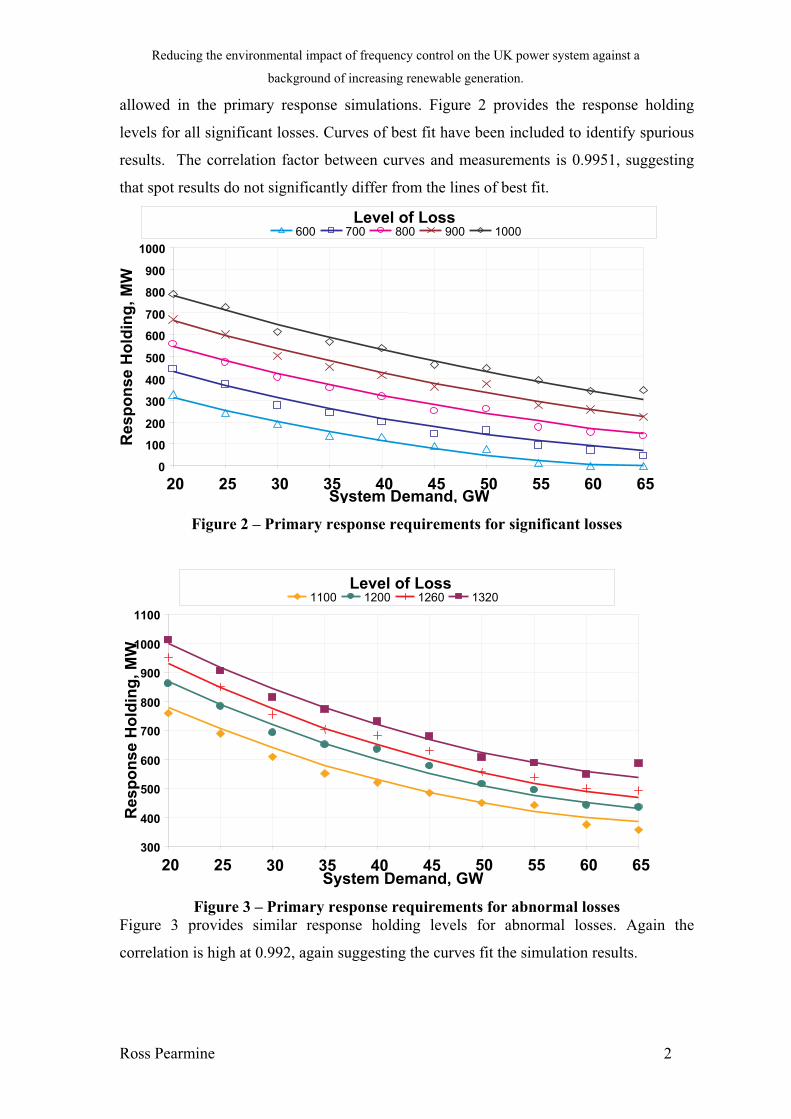
Reducing the environmental impact of frequency control on the UK power system against a
background of increasing renewable generation.
Ross Pearmine 2
allowed in the primary response simulations. Figure 2 provides the response holding
levels for all significant losses. Curves of best fit have been included to identify spurious
results. The correlation factor between curves and measurements is 0.9951, suggesting
that spot results do not significantly differ from the lines of best fit.
Figure 2 – Primary response requirements for significant losses
Figure 3 – Primary response requirements for abnormal losses
Figure 3 provides similar response holding levels for abnormal losses. Again the
correlation is high at 0.992, again suggesting the curves fit the simulation results.
0
100
200
300
400
500
600
700
800
900
1000
20 25 30 35 40 45 50 55 60 65System Demand, GW
Resp
on
se H
old
ing
, M
W
600 700 800 900 1000Level of Loss
300
400
500
600
700
800
900
1000
1100
20 25 30 35 40 45 50 55 60 65
Resp
on
se H
old
ing
, M
W
1100 1200 1260 1320
System Demand, GW
Level of Loss

Reducing the environmental impact of frequency control on the UK power system against a
background of increasing renewable generation.
Ross Pearmine 3
1.2 Changes in the Response Requirements
-300
-200
-100
0
100
200
300
400
500
20 25 30 35 40 45 50 55 60 65
System Demand, GW
MW
ch
an
ge in
re
sp
on
se h
old
ing
levels
1320
1260
1200
1100
1000
900
800
700
600
Figure 4 – Changes in primary response requirements (without margin)
Figure 4 shows the general trends of the current primary response requirements not
including a margin, against values calculated in this chapter. The simulations show that
the lower system demands generally require less primary response than operational
requirements suggest at present. In contrast, for the higher system demands response is
currently under provided by up to 400MW. Significant losses on the whole show a
reduction in requirements or no change at all, except at the higher system demands.
Abnormal losses require additional response according to the newly simulated values.
Secondary response requirements are identical to current values and so are not
considered.
1.3 Wind Turbine Model
The last report established significant problems in obtaining data to validate suitable wind
turbine models for simulations studies. The decision to use existing models from literate
sources to represent doubly fed induction machines was seen as a suitable compromise.
Figure 5 depicts the general structure of the variable speed wind turbine model with a
doubly fed induction generator. Each element of the model for the basis of this research is
presented in a relatively low level of detail. Full details of the model can be found in
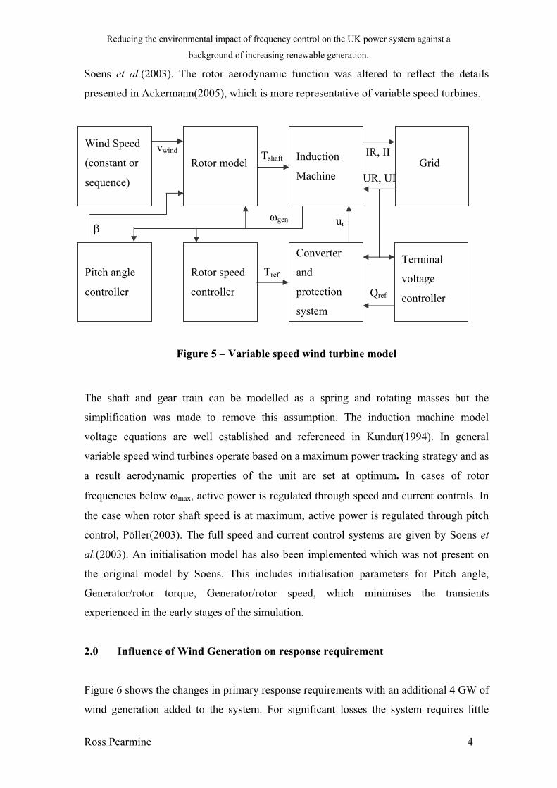
Reducing the environmental impact of frequency control on the UK power system against a
background of increasing renewable generation.
Ross Pearmine 4
Soens et al.(2003). The rotor aerodynamic function was altered to reflect the details
presented in Ackermann(2005), which is more representative of variable speed turbines.
Figure 5 – Variable speed wind turbine model
The shaft and gear train can be modelled as a spring and rotating masses but the
simplification was made to remove this assumption. The induction machine model
voltage equations are well established and referenced in Kundur(1994). In general
variable speed wind turbines operate based on a maximum power tracking strategy and as
a result aerodynamic properties of the unit are set at optimum. In cases of rotor
frequencies below max, active power is regulated through speed and current controls. In
the case when rotor shaft speed is at maximum, active power is regulated through pitch
control, Pöller(2003). The full speed and current control systems are given by Soens et
al.(2003). An initialisation model has also been implemented which was not present on
the original model by Soens. This includes initialisation parameters for Pitch angle,
Generator/rotor torque, Generator/rotor speed, which minimises the transients
experienced in the early stages of the simulation.
2.0 Influence of Wind Generation on response requirement
Figure 6 shows the changes in primary response requirements with an additional 4 GW of
wind generation added to the system. For significant losses the system requires little
Wind Speed
(constant or
sequence)
Rotor model Induction
Machine
Grid
Pitch angle
controller
Rotor speed
controller
Converter
and
protection
system
Terminal
voltage
controller
gen
Tshaft
vwind
ur
IR, II
UR, UI
Tref
Qref

Reducing the environmental impact of frequency control on the UK power system against a
background of increasing renewable generation.
Ross Pearmine 5
difference in primary response levels, however, there is a small increase in most cases.
The deviations notable in the 50 and 25 GW series are likely to be due to the chosen mix
of generation at that particular demand level affecting the system dynamics. Disregarding
these data points still allows a dominant trend to be established.
-250
-200
-150
-100
-50
0
50
100
20 25 30 35 40 45 50 55 60 65
Demand, GW
Ch
an
ge
s in
re
sp
on
se
req
uir
em
en
t, M
W
600
700
800
900
1000
1100
1200
1260
1320
Figure 6 – Changes in primary response requirements
For abnormal losses there is a general decrease in the primary response requirements.
This decrease is a result of the obligation to return to 49.5 Hz within one minute. In
previous simulations of the response requirements for the current generation mix this
factor was limiting the level of response. However, with lower system inertia as a result
of wind turbines displacing conventional plant, the system dynamics have changed. The
system is more susceptible to changes in frequency, and as a result the full frequency
deviation during primary timescales can be harnessed.
The reduction in response peaks at the 40 GW demand point, and falls off as demands
increase or reduce. This optimal point again results from the changes in system inertia. At
high demands the influence of wind turbine inertia is low due to a dominance of
conventional plant on the system. The total system inertia will become similar to the
current level experienced on the system as demands increase. Conversely, at low
demands the proportion of wind turbines to conventional plant is high. The total system
inertia becomes lower and as a result slightly more response is required to contain
frequency deviations within limits.

Reducing the environmental impact of frequency control on the UK power system against a
background of increasing renewable generation.
Ross Pearmine 6
-150
-100
-50
0
50
100
150
200
20 25 30 35 40 45 50 55 60 65
Demand, GW
Ch
an
ge
s in
re
sp
on
se
req
uir
em
en
t, M
W
600
700
800
900
1000
1100
1200
1260
1320
Figure 7 – Changes in secondary response requirements
Figure 7 gives changes in secondary response levels from the simulations with added
wind turbines. There is a noticeable peak in the 50 GW results series (except for the 600
and 1320 MW loss), which confirms that something untoward is occurring in this
particular system configuration. As explained earlier it is likely to be an effect of the
specific generation chosen to meet the demand level. Omitting these results, the general
trend of values is within around ±50 MW of the original simulations. This is typical of
some of the deviations noted in the simulations of the secondary response requirement in
section 1.1. This result is to be expected as the wind turbines should not significantly
affect the simulation under steady state conditions.
3.0 Demand Response
Figure 8 details the recorded load sensitivity to frequency from an additional 106 low
frequency incidents following generation loss. The results indicate a mean value of 3.43
%MW/Hz, however in the interests of security a worst case must be considered. The 15th
percentile from the line of best fit (derived from maximum likelihood estimation)
suggests a load sensitivity of 1.99 %MW/Hz, with a 95 percent confidence that the value
lies between 1.79 and 2.2. The results have shown that 85 percent of values calculated are
above a sensitivity of 2 %MW/Hz. This continues to give assurance in using this value as

Reducing the environmental impact of frequency control on the UK power system against a
background of increasing renewable generation.
Ross Pearmine 7
a minimum response expected from the load when used in conjunction with a margin in
the response requirement calculations.
Figure 8 - Distribution of load sensitivity to frequency
4.0 Targets from previous report
A number of milestones where met from the previous report including:
Implementation and Validation of a wind turbine model in Eurostag
Conclude review of response requirements
Complete response requirements adding a degree of wind power
Conduct sensitivity analysis
Write final thesis
Unfortunately it was not possible to conduct any live system tests with the updated
response requirement curves, due to the time required to give notice to all stakeholders.
The decision was also made not to translate response requirements into CO2 emissions.
Based on the work conducted, sufficient environmental benefit had been established. A
second paper was also submitted to the to Electric Power Systems Research journal with
minor revisions.
Sensitivity, %MW/Hz
Cu
mu
lati
ve
per
cen
t
0.1
0.1 1 10
0.51
510203050709099
Line of Best Fit Eq. 6.2
95 % Confidence limits
Load Sensitivity Eq. 6.2
99.9
1.99585 [1.7854,2.20173]
15.0
Eta Beta pve% n/s
3.866 2.748 23.32 187/0

Reducing the environmental impact of frequency control on the UK power system against a
background of increasing renewable generation.
Ross Pearmine 8
5.0 Summary
A complete dynamic response model was used to simulate the system response
requirements for safe and secure operation of the network under large infeed losses.
These results show some reduction in the primary response requirements is possible at
low system demands for significant losses (600-1000 MW). However, the simulations
also suggest that an increase in primary response holding is required at high system
demands for abnormal losses (>1000 MW). The secondary response requirements show
an overall reduction in the holding levels.
These simulations have shown that the existing system obligations under low frequency
events limit the potential reduction in primary response holding. The dynamic
requirement to return system frequency to 49.5 Hz in 60 seconds, in most cases, prevents
the system from reaching the minimum frequency. There is potential to reach the
minimum frequency under primary response timescales by allowing generators to provide
only secondary response. Alternatively, recommendations to extend the dynamic
requirement by a further minute would offer a more suitable transient frequency.
A doubly fed wind generator model was implemented from a number of research projects
to represent potential offshore wind farms around the British Isles. The wind farm models
were integrated with the complete dynamic model to assess changes in the response
requirements. As a result of a net decrease in the total system inertia significant losses
require up to 50 MW of additional primary response. The primary response holding for
abnormal is shown to be reduced by between 50 and 200 MW, dependant on loss and
system demands.
From the perspective of the system security this means there is no urgency in revising the
current response requirements as up to 8.5 GW of new wind generators are integrated
with the real system. The response margin should easily subsume an additional 50 MW
of primary response require in significant events, thus maintaining system security.
Under abnormal losses the system security should also be maintained with no further
actions. In the interests of system efficiency under abnormal losses, the operational
response requirements should be revised to realise any potential reductions in holding
levels.

Reducing the environmental impact of frequency control on the UK power system against a
background of increasing renewable generation.
Ross Pearmine 9
6.0 References
1. Ackermann, T., ‘Wind in power systems’, John Wiley & sons, Chichester, 2005,
Chap 25.
2. Pöller, M., and Achilles, S., ‘Aggregated Wind Park Models for Analyzing Power
System Dynamics’, Proc. 4th International Workshop on Large Scale Integration
of Wind Power and Transmission Networks for offshore wind farms, Billund,
2003.
3. Soens, J., Driesen, J., and Belmans, R., ‘A comprehensive model of a doubly fed
induction generator for dynamic simulations and power system studies’,
International conference on Renewable energies and power quality (ICREPQ),
Vigo, Spain, April 9-12, 2003.