Embed Size (px)
Citation preview

ROTATING TWO LEG BOSE HUBBARDLADDER
a thesis
submitted to the department of physics
and the institute of engineering and science
of bilkent university
in partial fulfillment of the requirements
for the degree of
master of science
By
Ahmet Keles
August, 2009

I certify that I have read this thesis and that in my opinion it is fully adequate,
in scope and in quality, as a thesis for the degree of Master of Science.
Assoc. Prof. Dr. M. Ozgur Oktel (Supervisor)
I certify that I have read this thesis and that in my opinion it is fully adequate,
in scope and in quality, as a thesis for the degree of Master of Science.
Prof. Dr. Cemal Yalabık
I certify that I have read this thesis and that in my opinion it is fully adequate,
in scope and in quality, as a thesis for the degree of Master of Science.
Assoc. Prof. Dr. Azer Kerimov
Approved for the Institute of Engineering and Science:
Prof. Dr. Mehmet B. BarayDirector of the Institute Engineering and Science
ii

ABSTRACT
ROTATING TWO LEG BOSE HUBBARD LADDER
Ahmet Keles
M.S. in Physics
Supervisor: Assoc. Prof. Dr. M. Ozgur Oktel
August, 2009
We analyze two leg Bose Hubbard model under uniform magnetic field within var-
ious methods. Before studying the model, we discuss the background on rotating
Bose Einstein condensates, Bose Hubbard model and superfluid Mott insulator
transition. We give a general overview of Density Matrix Renormalization Group
(DMRG) theory and show some of the applications. Introducing two leg system
Hamiltonian, we solve the single particle problem and find distinct structures
above and belove a critical magnetic field αc = 0.21π. Above this value of the
field, it is found that system has travelling wave solutions. To see the effects
of interactions, we use Gross Pitaevskii approximation. Spectrum of the system
below the critical field and the change of αc with the interaction strength are ob-
tained for small interactions, i.e Un/t < 1. To specify Mott insulator boundary,
variational mean field theory and strong coupling perturbation (SCP) theories
are used. The travelling wave solutions found in single particle spectrum above
αc is found to be persistent in mean field description. On the other hand, com-
paring with the strong coupling expansion results, it has been found that the
mean field theory gives poor results, because of the one dimensional structure
of the system. The change of the tip of the lobe where BKT transition takes
place is found as a function of magnetic field by SCP. Finally we use DMRG to
obtain the exact shape of the phase diagram. It is found that second order strong
coupling perturbation theory gives very good results. System is found to display
reenterant phase to Mott insulator. Looking at the infinite onsite interaction
limit via DMRG, the critical value of the magnetic field is found to be exactly
equal to the single particle solution. We have calculated the particle-hole gap for
various fillings and different magnetic fields and found Fractional Quantum Hall
like behaviors.
Keywords: Bose-Hubbard Model, Superfluid-Mott Insulator Transition, Renor-
malization, Strongly Correlated Systems.
iii

OZET
DONEN IKILI BOSE HUBBARD MERDIVENI
Ahmet Keles
Fizik, Yuksek Lisans
Tez Yoneticisi: Yard. Doc. Dr. M. Ozgur Oktel
Agustos, 2009
Duzgun manyetik alan altındaki iki bacaklı Bose Hubbard modeli farklı
yontemlerle analiz edildi. Bu model calısılmadan once, donen Bose Einstein
yogusuklarının, Bose Hubbard modelinin ve superakıskan Mott yalıtkanı gecisinin
arka planı tartısıldı. Yogunluk Matrisi Renormalizasyon Grubu (YMRG) teorisi
genel olarak anlatıldı ve bazı uygulamaları gosterildi. Iki bacaklı sistemin
Hamiltonyeni verildikten sonra, tek parcacık problemi cozuldu ve kritik bir
manyetik alanının αc = 0.21π altında ve ustunde birbirinden farklı yapılanmalar
bulundu. Kritik manyetik alanın bu degerinin uzerinde, hareketli dalga cozumleri
bulundu. Etkilesimlerin etkilerini gormek icin, Gross Pitaevskii yaklasımı kul-
lanıldı. Sistemin kritik manyetik alan altındaki spektrumu ve αc’nin etkilesim
kuvvetiyle degisimi zayıf etkilesimler icin, Un/t < 1, bulundu. Mott yalıtkanı
sınırının belirlenmesi amacıyla ortalama alan ve guclu baglasım perturbasyonu
(GBP) teorileri kullanıldı. Tek parcacık spektrumunda bulunan, kritik manyetik
alan uzerindeki hareketli dalga cozumlerinin ortalama alan teorisinde de kul-
lanılması gerektigi goruldu. Diger yandan, guclu baglasım teorisiyle karsılastırma
sonucunda, sistemin bir boyutlu yapısından da dolayı, ortalama alan teorisinin
kotu sonuc verdigi bulundu. BKT gecisinin oldugu, Mott yalıtkanı alanlarının
tam uc noktasının manyetik alan ile degisimi GBP ile bulundu. Son olarak,
YMRG kullanılarak faz diyagramının kesin sekli elde edildi. Bu sonuclarla ikinci
dereceye kadar yapılan GBP sonuclarının cok iyi oldugu goruldu. Sistemin Mott
yalıtkanı fazına geri-giris gosterdigi goruldu. Sonsuz site-ici etkilesimine YMRG
ile bakılarak, manyetik alanın kritik degerinin tek parcacık cozumune tam alarak
esit oldugu goruldu. Parcacık-bosluk enerji aralıgı degisik dolum oranlarınında
ve manyetik alanlarda hesaplandı ve Kesirli Kuantum Hall Etkisine benzeyen
davranıslar gozlemlendi.
Anahtar sozcukler : Bose-Hubbard Modeli, Superakıskan-Mott Yalıtkanı Gecisi,
Renormalizasyon, Guclu Baglasık Sistemler.
iv

Contents
1 Introduction 1
1.1 BEC: General Overview . . . . . . . . . . . . . . . . . . . . . . . 1
1.1.1 Gross Pitaevskii Equation . . . . . . . . . . . . . . . . . . 4
1.2 Superfluidity and Rotating Condensates . . . . . . . . . . . . . . 5
1.3 Landau Levels and Quantum Hall Regime . . . . . . . . . . . . . 7
1.4 Outline of the Thesis . . . . . . . . . . . . . . . . . . . . . . . . . 10
2 Bose Hubbard Model 11
2.1 Superfluid Mott Insulator Transition . . . . . . . . . . . . . . . . 12
2.2 Mean Field Theory . . . . . . . . . . . . . . . . . . . . . . . . . . 14
2.3 Strong Coupling Expansion . . . . . . . . . . . . . . . . . . . . . 16
2.4 Rotation in Bose Hubbard Model . . . . . . . . . . . . . . . . . . 21
3 Density Matrix Renormalization Group 22
3.1 Exact Diagonalization . . . . . . . . . . . . . . . . . . . . . . . . 23
3.2 Density Matrix . . . . . . . . . . . . . . . . . . . . . . . . . . . . 24
v
CONTENTS vi
3.2.1 Reduced Density Matrix . . . . . . . . . . . . . . . . . . . 26
3.2.2 Density Matrix Truncation . . . . . . . . . . . . . . . . . . 27
3.3 DMRG Algorithms . . . . . . . . . . . . . . . . . . . . . . . . . . 29
3.3.1 Infinite System Algorithm . . . . . . . . . . . . . . . . . . 30
3.3.2 Finite System Algorithm . . . . . . . . . . . . . . . . . . . 32
3.4 Applications . . . . . . . . . . . . . . . . . . . . . . . . . . . . . . 34
3.4.1 Heisenberg Model . . . . . . . . . . . . . . . . . . . . . . . 34
3.4.2 Bose-Hubbard Model . . . . . . . . . . . . . . . . . . . . . 41
3.5 Conclusion . . . . . . . . . . . . . . . . . . . . . . . . . . . . . . . 48
4 Two Leg Bose Hubbard Model 50
4.1 Single Particle Spectrum . . . . . . . . . . . . . . . . . . . . . . . 51
4.2 Gross-Pitaevskii Approximation . . . . . . . . . . . . . . . . . . . 53
4.3 Variational Mean Field Approach . . . . . . . . . . . . . . . . . . 57
4.4 Strong Coupling Expansion . . . . . . . . . . . . . . . . . . . . . 61
4.5 DMRG Calculations . . . . . . . . . . . . . . . . . . . . . . . . . 64
4.6 Evidence of Strongly Correlated Phases . . . . . . . . . . . . . . . 66
4.7 Conclusion . . . . . . . . . . . . . . . . . . . . . . . . . . . . . . . 71
List of Figures
2.1 The order parameter calculated from self consistent meanfield ap-
proximation as a function of chemical potential µ and hopping t is
shown on the left. The superfluid fraction as hopping in increased
is shown on the right for two different chemical potentials. . . . . 15
2.2 Phase diagram of one dimensional Bose Hubbard Model calculated
from strong coupling perturbation up to second order. . . . . . . . 20
3.1 Schematic representation of a system composed of two parts A
and B. |i〉 and |j〉 are the complete sets of states that span each
subsystem. . . . . . . . . . . . . . . . . . . . . . . . . . . . . . . . 27
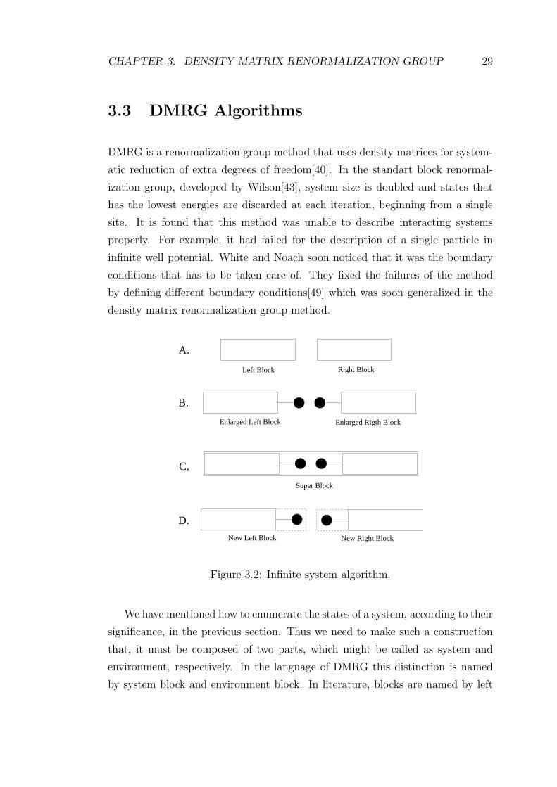
3.2 Infinite system algorithm. . . . . . . . . . . . . . . . . . . . . . . 29
3.3 Convergence of the energy to the exact value is shown in the left
pane and the decay of eigenvalues of the density matrix is in the
right panel for M=24 states kept. . . . . . . . . . . . . . . . . . . 38
3.4 Sparseness of the superblock and the left enlarged block respectively. 39
3.5 Energy per site as a function of system size is on the left for spin-
1 system with open boundary conditions. On the right decay of
density matrix eigenvalues are shown . . . . . . . . . . . . . . . . 41
vii

LIST OF FIGURES viii
3.6 Haldane gap for spin-1/2 system as a function of inverse system
size on the left and the one for spin-1 system as a function of inverse
system size squared on the right. Gap is defined as the difference
between ground state and the first excited state ∆1/2 = E1 − E0
for spin-1/2 and difference between first and second excited states
∆1 = E2 − E1 for spin-1. . . . . . . . . . . . . . . . . . . . . . . . 42
3.7 Ground state energies versus inverse system size of Bose Hubbard
model for Mott state and particle-hole defect states for two differ-
ent values of hopping parameter,J = 0.001 (on left) and J = 1 (on
right). Red straight lines are linear fits to DMRG points. . . . . . 45
3.8 Eigenvalue spectrum of the density matrices in Bose Hubbar model
DMRG for two different values of hopping strength. . . . . . . . . 46
3.9 Gap multiplied by size vs hopping strength for different system
sizes with M = 30 states kept. Coalescence of curves for different
lengths shows the transition to superfluid. Transition is Kosterlitz-
Thouless type. . . . . . . . . . . . . . . . . . . . . . . . . . . . . . 47
3.10 Phase diagram of one dimensional Bose hubbard model with onsite
interaction. M = 30 states are kept in the dmrg iteration for a
system of size L = 50. The BKT phase transition is not seen
because of the method used which is mentioned in the text. . . . . 48
4.1 Single particle band diagram two leg ladder under magnetic field.
Left pane is plotted for α = 0 whereas right pane is for α = 0.4.
The band gap between the conduction and the valance bands is
zero for the left which is nonzero for the right. . . . . . . . . . . 53

LIST OF FIGURES ix
4.2 Band minimums (dashed blue for the conduction band and solid
green for the valance band) and band maximums (solid blue for
the conduction band and dashed green for the valance band) as a
function of magneticfield. Analog of Hofstadter butterfly for two
leg ladder. A finite gap between conduction and valance band
appears at α = 1/3 . . . . . . . . . . . . . . . . . . . . . . . . . . 54
4.3 Band diagrams for two leg ladder with onsite interactions calcu-
lated from the Gross Pitaevskii approximation. Solid lines are for
U = 0 and dotted lines are for U = 0.5. Left panel is for zero
magnetic field and the right panel is for α = 0.2 . . . . . . . . . . 56
4.4 Change of critical magnetic field with the increase of interaction
strength for low values of U , that is Un/t < 1. Plot is scaled with
t = 1 and n = 1. In the limit U → 0, αc goes to the previously
obtained value from the single particle solutions. Inset shows the
behavior for large values of U , which is not reliable because of
strong interactions. . . . . . . . . . . . . . . . . . . . . . . . . . . 57
4.5 Mott phase boundary is shown on the left as a function of magnetic
field strength and the chemical potential. Unlike two dimensional
case, boundary is perfectly smooth. On the right, result of the
minimization of the energy with respect to phase parameter θ in
Eq.(4.12) is shown. It is seen that above the critical magnetic
field, the minimum energy ansatz bears complex amplitudes as in
the case of single particle solution. . . . . . . . . . . . . . . . . . 60
4.6 Labelling of sites in two leg ladder for the calculation of strong
coupling expansion . . . . . . . . . . . . . . . . . . . . . . . . . . 61

LIST OF FIGURES x
4.7 Phase diagram of two leg ladder, shown on the left, from strong
coupling perturbation theory for magnetic fields α = 0, α = 0.2
and α = 0.4 compared with the results of meanfield calculation
(dotted thin lines). Above α = 0.43 lines of µP and µH does not
cross and higher oder perturbation is required. On the left the tip
of the Mott region is shown as a function of field. Thin line after
α = 0.43 is spline interpolant. . . . . . . . . . . . . . . . . . . . . 63
4.8 Phase diagram of two leg Bose Hubbard ladder for α = 0 on the
left and α = 0.45 on the right. For comparison strong coupling
results are also shown. . . . . . . . . . . . . . . . . . . . . . . . . 65
4.9 Gap between ground state and two excited states for different mag-
netic field. The gap between first excited state E1 − E0 is shown
by green ’+’, whereas the one for E2 − E0 is shown by blue ’’.Thin lines are spline interpolation to data points. It is seen that
around αc = 0.21 spectrum has a jump to a completely different
behavior. . . . . . . . . . . . . . . . . . . . . . . . . . . . . . . . . 68
4.10 Energy gap defined in Eq.4.23 as a function of particle density for
α = 1/3 in the first figure, 2/5 in the second and 1/2 in the third
respectively. For each value of α, a different peak is seen in the
energy gap where the peaks are symmetric around 0.5. Apart from
the dominant peaks at 1/5, 1/6 for α = 1/3, 1/5, 4/5 for α = 2/5
and 1/4, 3/4 α = 1/2 and the persistent peak at 1/2, there seem
to be fluctuating non zero gap value for other fillings. . . . . . . . 69
List of Tables
1.1 Landau level index and corresponding angular momentum index
for a two dimensional rotating condensate with isotropic harmonic
confinement along the plane. The degeneracy increases as the en-
ergy eigenvalue is increased. . . . . . . . . . . . . . . . . . . . . . 8
3.1 Difference between energy calculated from exact diagonalization
and the energy of DMRG calculation for a finite size, L=8 site
system. . . . . . . . . . . . . . . . . . . . . . . . . . . . . . . . . . 41
4.1 Value of the filling factor defined in Eq.4.24 for different magnetic
fields shown in Fig.4.10 . . . . . . . . . . . . . . . . . . . . . . . . 70
xi

Chapter 1
Introduction
Achievement of Bose Einstein condensation (BEC) has made a revolution in the
development of many body physics in both theoretical and experimental studies.
Being born at the intersection of disciples like Quantum Optics, Condensed Mat-
ter Physics and Atomic Physics, BEC has grown out to be a totally new branch
of physics. In this chapter, we are going to give a short introduction to the basic
concepts, generally discussing the theoretical foundation of the phenomena and
consider the effect of fast rotation.
1.1 BEC: General Overview
Wave function describing a collection of identical quantum particles is either
symmetric or anti-symmetric under the exchange of two particles. This exchange
symmetry comes from the indistinguishability of the particles and separates the
nature into two different class of statistics. Bosons are identified by the inte-
ger total spin and obey the Bose Einstein distribution, whereas fermions have
half integer spin and obey Fermi Dirac distribution. For fermions, there is an
exchange force coming from the antisymmetry of the wavefunction. It prevents
two particles from occupying the same energy level and called Pauli exclusion
principle. On the other hand, there is no such constraint for bosons so that
1

CHAPTER 1. INTRODUCTION 2
infinitely many particles can be placed in the same energy eigenstate. Though
fermions have interesting physics, we are mainly interested in bosons, particularly
the macroscopic occupation of a single eigenstate in this thesis.
For a collection of bosonic atoms, having energy eigenstates Ei, the occupation
number of each state is given by the Bose Einstein statistics
〈ni〉 =1
eβ(Ei−µ) − 1(1.1)
where β = 1/kT is the inverse temperature, k is Boltzmann constant and µ is
the chemical potential. In the limit of low temperature (T → 0 or β → ∞) the
exponential term diverges and the occupation number of each state goes to zero so
that one of the states must be filled separately. It is a standart textbook exercise
to make this argument more quantitative. Defining the external potential to
provide the exact energy spectrum and the dimensionality, a critical temperature
where particles settle down to the ground state can be found [1, 2]. Another
simple approach to see the peculiarity about absolute zero can be obtained by
comparing the kinetic energies of particles (p2/2m) with the thermal energy (kT )
via the help of De Broglie relation λ = h/p (h is Planck’s constant). One can
obtain a relation of the form λ ∝√
h2/2mkT . Thus as the temperature of the
system goes to zero, particles will have a giant matter wave structure [3, 4].
BEC is defined as the macroscopic occupation of one of the single particle
energy levels. Let Ψs(x1, x2, . . . , xN ) be set of many-body wavefunctions of a
collection of N particles which is symmetric under the exchange of two particles,
with weights ws. Single particle reduced density matrix is defined as[5]
ρ1(x, y) = N∑
s
ws
∫
dx2dx3 . . . dxNΨ∗s(x, x2, . . . , xN)Ψs(y, x2, . . . , xN) (1.2)
where we have assumed one dimensional system for simplicity but this can be
extended to three dimension and time dependence can be considered. From
Eq.(1.2) it is seen that the density matrix ρ1(x, y) is Hermitian, thus it can be
put into a diagonal form,
ρ1(x, y) =∑
i
niφ∗i (x)φi(y) (1.3)

CHAPTER 1. INTRODUCTION 3
where φ is the complete set of orthogonal states. The coefficients in this expansion
can be found by exploiting the orthogonality 〈φn|φm〉 = δnm as
ni =
∫
φ∗(y)ρ1(x, y)φ(x)dxdy. (1.4)
Formal definition of BEC : If one of the eigenvalues n0 in Eq.(1.3) is order of
total number of particles so that, sum in Eq.(1.3) has to be done by separating
the dominant term[6]; like ρ1(x, y) = n0φ∗0(x)φ0(y) +
∑
i6=0 niφ∗i (x)φi(y), then the
system is said to be Bose condensed[5, 6, 7]. Accumulation of particles on one
of the single particle eigenstates enables a simple form for the many body wave
function. Condensate wave function can be written as
Φ(r) =√Nψ0(r) (1.5)
where it is normalized to the total number of particles. In this expression, ψ0(r)
is a complex valued function and called order parameter. One can safely write
this function of the form ψ0(r) = |ψ0(r)|eiθ, where θ is a function of r.
To extend the discussion further, it is necessary to introduce system Hamil-
tonian. Hamiltonian for a system of N particles interacting via the two body
interatomic potential V (r − r′) is given in second quantization
H =
∫
drΨ†(r)H0Ψ(r) +1
2
∫
drdr′Ψ†(r)Ψ†(r′)V (r − r′)Ψ(r)Ψ(r′) (1.6)
where Ψ(r) and Ψ†(r) are bosonic field operators that create and annihilate a
particle at position r which satisfy the commutation [Ψ(r), Ψ†(r)] = δ(r− r′), all
other commutators being zero, and H0 is the noninteracting part of the Hamil-
tonian given by H0 = ~2∇2/2m + Vext(r). The term Vext(r) in H0 is external
potential which is generally a harmonic oscillator potential. For a dilute gas
at low temperature the interaction comes from two body collisions and given
by[1, 5, 8]
V (r − r′) =4π~
2a
mδ(r − r′) (1.7)
where a is the s-wave scattering length.

CHAPTER 1. INTRODUCTION 4
1.1.1 Gross Pitaevskii Equation
A first strike at Eq.(1.6) is the exploitation of the mean field approximation. This
is essentially nothing but the replacement of the field operator with a classical
field such as Eq.(1.5). To obtain the equation of motion, one uses Heisenberg
equation i~∂Ψ/∂t = [Ψ, H ] which gives
i~∂Φ(r, t)
∂t= −~
2∇2
2mΦ(r, t) + Vext(r)Φ(r, t) +
4π~2a
m|Φ(r, t)|2Φ(r, t). (1.8)
This equation is called Gross-Pitaevskii equation. As long as the diluteness con-
dition na3 ≫ 1 (n is density of the condensate and a is s-wave scattering length)
is satisfied, this equation describes the condensate precisely in zero temperature
limit[1, 8]. Assuming a time dependence of the form Φ(r, t) = Φ(r)e−iµt/~ in the
wavefunction, time independent Gross-Pitaevskii equation can be obtained as[
−~2∇2
2m+ Vext(r) + g|Φ(r)|2
]
Φ(r) = µΦ(r) (1.9)
where µ is the chemical potential and g = 4π~2a/m. Eq.(1.9) is a nonlinear
Schrodinger equation and exact solution is not always possible. There are several
approaches for the approximate solution that will be mentioned briefly.
The first approach is variational, which is sometimes called ideal gas approx-
imation. Having a solution to the non-interacting part of the Hamiltonian, a
variational wavefunction can be defined that will minimize the energy. For an
example, if the external potential is a harmonic oscillator potential, than the
non-interacting part of the Hamiltonian will have a gaussian wave function in the
ground state. Thus, defining a parameter dependent gaussian function that is
properly normalized, one can obtain an upper limit for the energy. This method
is proved to be very accurate to describe both the ground state properties and
the collective excitations of Bose Einstein condensates.
Second approach is called Thomas-Fermi approximation. For sufficiently large
number of atoms, the kinetic energy is much less than the interaction and poten-
tial energies. Thus one can ignore the kinetic energy term and solve the remaining
algebraic equation for the chemical potential. Other quantities such as the total
energy and the radius of the condensate can be obtained with this method.

CHAPTER 1. INTRODUCTION 5
Literature on Gross Pitaevskii equation is pretty diverse and we have not men-
tioned most of the important methods like numerical solutions or soliton solutions.
Gross Pitaevskii theory is one of the very strong approaches for the analytical
treatment of Bose Einstein condensates and a detailed analysis can be obtained
from the references[1, 8]. A higher order approximation to Gross Pitaevskii the-
ory is the so called Bogoliubov theory. Looking at small perturbations around
the equilibrium wave function, one can consider the following[9]
Ψ = Φ + ueiwt + ve−iwt (1.10)
and the excitation spectrum at higher order can be obtained.
1.2 Superfluidity and Rotating Condensates
Superfluidity was discovered by Kamerlingh Onnes with the experiments on He at
low temperatures. Helium 4 is a superfluid that shows unusual properties below
a specific temperature called lambda point, it has zero viscosity that diminishes
the friction between the liquid and the container, zero entropy and infinite heat
conductivity. These properties cause the liquid to display extraordinary proper-
ties. For example, superfluid helium can pass through very thin capillaries that
it cannot pass above the lambda point. Another example is that the superfluid
He can flow up through a tube plunged into it, which is called fountain effect.
Among these surprises, the effect of rotation on superfluids is in particular in-
terest of this thesis. If the container is rotated up to some particular angular
velocity, superfluid does not rotate but stands still, whereas a classical fluid is
expected to rotate. An interesting observation is the following. Assume that the
container is rotated while the temperature is above the lambda point of Helium.
Since temperature is not low enough, the fluid is classical and will rotate with the
container. If the temperature is lowered below the transition temperature while
it is still in rotation, the fluid will go on rotation to conserve the angular mo-
mentum. However, if the container is stopped, the superfluid will keep rotating
without any change, indefinitely[7].
These unusual properties are later explained to be quantum mechanical by

CHAPTER 1. INTRODUCTION 6
Landau with his theory of quasiparticle excitations in liquid Helium[10]. The
superfluidity of liquid helium comes from the partial Bose Einstein condensation
that has taken place below lambda point. Though fraction of condensation (about
%10) is pretty low, Bogoliubov approximation outlined in the previous section
successfully describes its behavior[11].
We can figure out the effect of rotation on Bose Einstein condensates by using
the condensate wave function. The order parameter defined in Eq.(1.5) is used
to find particle current density
J =~
2mi[ψ∗
0∇ψ0 − ψ0∇ψ∗0] (1.11)
which can be found as J = ~n0∇θ/m where n0 = |ψ0|2 is the density. Using the
relation J = nv the superfluid velocity can be found as
vs =~
m∇θ. (1.12)
It follows from Eq.(1.12) that a superfluid defined by this order parameter is
irrotational ∇× vs = 0, because curl of a gradient is zero for any function. An
important consequence of this irrotationality follows from the surface integration
of curl of the velocity field, which is defined as the circulation. Circulation is
defined as: κ =∫
S∇×vs ·ndS, where n is the unit vector normal to the surface.
Using Stokes theorem it can be written as κ =∮
Cdl ·vs =
∮
Cdl ·∇θ. Considering
the single-valuedness of the wave function, the following relation can be obtained;
κ =2π~
ml (1.13)
which is called quantization of the circulation and l is an integer. This identity is
the basis of irrotationality of the superfluid. It requires the quantized circulation
which gives rise to formation of quantized vorticity in rotating superfluids. For
the example of superfluid helium, the liquid does not respond to rotations upon
small angular momentum. Whenever the critical rotation frequency is reached,
a sudden vortex formation appears that carries a quantized angular momentum
and a quantized circulation as given above. As the rotation frequency increases,
the number of vortices increases. In the limit of fast rotations, these vortices form
a regular array called vortex lattice. The meaning of fast rotation will be precise

CHAPTER 1. INTRODUCTION 7
in the next section. Vortex and vortex lattice formations are experimentally
achieved in both superfluid Helium and Bose Einstein condensates of alkali metal
gases.
The theory of vorticity in superfluids has remarkable similarities between the
vorticity in superconductors. The analogy of irrotationality in superconductivity
is the absence of a magnetic field inside a superconductor . It gives rise to the
so called Meissner Effect. The magnetic field inside a superconductor vanishes
but increasing the strength of the magnetic field, singularities start to form that
magnetic field can pass through. In the limit of strong magnetic field, these
singularities start to form a regular lattice which is called Abrikosov vortex lattice.
1.3 Landau Levels and Quantum Hall Regime
For a rotating condensate under the harmonic oscillator potential, the single
particle Hamiltonian H0, defined in Eq.(1.6) can be written as
H0 =p2
2m+
1
2mw2r2 − ΩLz (1.14)
in the rotating frame of reference. For simplicity we assume a two dimensional
condensate, trapped in a two dimensional isotropic potential. This assumption
could be made much more subtle by considering a three dimensional condensate
strongly trapped along z direction, but we will not consider this here for simplicity.
The angular momentum operator is Lz = xpy − ypx, Ω is the frequency of the
rotation and x, px obey the commutation [x, px] = i~ (similar for y components).
The creation and annihilation operators are defined as
ax =1√2~
(mωx+ ipx)
ay =1√2~
(mωy + ipy) (1.15)

CHAPTER 1. INTRODUCTION 8
Table 1.1: Landau level index and corresponding angular momentum index for atwo dimensional rotating condensate with isotropic harmonic confinement alongthe plane. The degeneracy increases as the energy eigenvalue is increased.
N M
0 01 1, -12 -2, 0, 23 -3, -1, 1, 3
which satisfy the commutations [ax, a†x] = 1 and [ay, a
†y] = 1, all other commuta-
tors being zero. Thus, the Hamiltonian in Eq.(1.14) can be cast into the form,
H
~ω= (a†xax + a†yay + 1) + i
Ω
ω(a†xay − axa
†x)
=(
a†x a†y
)
(
1 iΩ/ω
−iΩ/ω 1
)(
ax
ay
)
+ 1. (1.16)
Diagonalization of 2×2 matrix in Eq.(1.16) is simple which gives the eigenvalues
λ1,2 = 1 ± Ω/ω. Thus the energy eigenvalues of the Hamiltonian can be written
as,
En,m = ~(ω + Ω)n+ ~(ω − Ω)m+ ~ω (1.17)
where n and m are integers for band indices. In this form it is easy to see that
the index n gives the main separation between the energy levels and it is called
Landau Level index. The case n = 0 is called the lowest Landau level (LLL).
It is interesting to consider the case Ω → ω which is called the rapid rotation
limit introduced in previous section. In this case dependence of the energy to
m vanishes and each Landau level becomes highly degenerate. In this limit, the
separation between the lowest Landau levels become exactly 2~ω.
It is often convenient to separate the energy coming from angular momentum
in Eq.(1.17). Energy can be written as En,m = ~ω + ~ω(n + m) − ~Ω(m − n)
and new indices N = n + m, M = m − n can be introduced. In this form,
E ∼ ~ωN − ~ΩM , where N in the index of the energy level and M is the
angular momentum number. Three different regions can be identified along with
this form of the eigenstates[9]: i- Weak Rotation(Ω ≈ 0): The energy levels

CHAPTER 1. INTRODUCTION 9
depend only on the index N and each state shown in Table.1.1 is degenerate
within the allowed angular momentum quantum numbers. The degeneracy is
splitted for small values of angular frequency. ii- Moderate Rotation(Ω > 0): The
degeneracies of the weak rotation is now removed because of the Coriolis force
coming from the angular momentum. iii- Fast Rotation(Ω ≈ ω): A degeneracy
different from the weak rotation comes out and the separation of energy levels is
2~ω. The amount of angular momentum imposed on the condensate is very large
and the gas forms a uniform array of quantized vortices (vortex lattice) to carry
this angular momentum. This regime is sometimes called meanfield quantum
Hall regime.
To see the effect of Coriolis force, another approach[12, 13] is performed to the
Hamiltonian in Eq.(1.14). It can be shown that the following form is equivalent
to the Hamiltonian in Eq.(1.14)
H =(p− A)2
2m+
1
2m(ω2 − Ω2)r2 (1.18)
where A is the vector potential A = mΩ × r. This form is identical to the
Hamiltonian of a charged particle in a magnetic field. This shows that the rotation
decreases the effect of the harmonic confinement. The strength of Coriolis force is
limitted by the oscillator frequency. In the limit Ω → ω, it cancels the harmonic
confinement and the condensate flies apart.
It is an experimental challenge to put the condensate in the meanfield quantum
Hall regime. In the current experiments, rotation frequency attained is 99%
of the oscillator frequency[14]. The difficulty of rapid rotation comes from the
upper limit set by the harmonic trap. There are, on the other hand, some works
that propose to add a quadric potential to the harmonic trap which has been
shown to indicate promising implications like a giant vortex formation or the
entrance to the quantum Hall regime[15]. Another direction for the exploration
of fast rotation limit is the use of optical lattices[16]. Considering a condensate
loaded on a rotating optical lattice, it is possible to reach extremely fast rotation
rates, which is experimentally achieved[17]. On the other hand, Description of
rotating condensates in optical lattice is a difficult theoretical problem which we
will mention extensively throughout the thesis.

CHAPTER 1. INTRODUCTION 10
1.4 Outline of the Thesis
In this thesis, we aim to study the nature of a fast rotating Bose Einstein conden-
sate extensively. To provide fast rotation and get rid of the limit set by harmonic
confinemet, we will focus on the condensates in optical lattices, which is described
via the Bose Hubbard model. We will consider a toy model, two leg ladder, that
mimics the characteristic properties of rotating Hubbard model. Though the
model is in its simplest form, theoretical explanation of its physical properties
is a challenge. For this reason, we have employed a bunch of theoretical and
numerical methods for a reliable description.
The thesis is organized as follows: In Chapter 2 we will introduce the Bose
Hubbard model and its basic property; the superfluid Mott insulator transition.
We show its well established theoretical treatments within the mean field and the
perturbation approximations. In Chapter 3, we will make a review of the density
matrix renormalization group theory (DMRG) and show basic algorithms applied
to one dimensional spin systems. Application of DMRG to Bose Hubbard model
will be presented and the derivation of the superfluid Mott insulator transition
will be shown. Finally, in the last part, Chapter 4, we will use all of these methods
to analyze the rotating two leg Bose Hubbard ladder. It will be shown that system
bears evidence of strongly correlated states.

Chapter 2
Bose Hubbard Model
Bose Hubbard Hamiltonian is a model that describes strongly correlated systems
under periodic boundary conditions. This periodicity may come from the crystal
structure or the periodic optical confinement of atoms in Bose Einstein conden-
sates. It can be applied to a variety of bosonic or fermionic systems such as
electrons in the semiconductor crystal, liquid helium, Josephson junction arrays
and Bose Einstein condensates in optical lattices. Apart from the diversity of
applications, the model is valid under both weakly and strongly interacting re-
gions irrespective of the correlations included. Unfortunately an exact solution
to this model is only possible under special circumstances, particularly for low
dimensional systems like Bethe Ansatz solution. There are, however, very strong
theoretical and numerical approaches valid in a wide range of system parame-
ters. Some of them are the central point of this thesis and will be investigated
in detail. In this chapter, this model will be introduced in the context of Bose
Einstein condensates loaded onto optical lattices. Basic theoretical approaches
will be presented like a mean field approximations and a perturbative expansion.
An important property of the model, i.e superfluid to Mott insulator transition
will be investigated extensively within those approximations.
11

CHAPTER 2. BOSE HUBBARD MODEL 12
2.1 Superfluid Mott Insulator Transition
Bose Hubbard model is analyzed by Fisher et al.[18] in a more general form and
interplay between the superfluid and Mott insulator phases is introduced for the
first time by using scaling theory to mainly study the criticality. Upon Jaksch et
al.’s work[19] which shows the possibility of realization of Bose Hubbard model
in Bose Einstein condensates on optical lattices, the model has taken a new di-
rection towards the study of degenerate quantum gases. In [20], phase diagram is
obtained within different meanfield approaches and failure of Bogoliubov approx-
imation is shown which indicates the importance of interactions and correlations
in optical lattices. The superfluid to Mott insulator transition is observed ex-
perimentally by Greiner et al.[21]. This work placed Bose Hubbard model in the
center of researches on the strongly correlated systems[22, 23].
Bose Hubbard Hamiltonian is written as
H = −∑
〈i,j〉
tija†iaj +
U
2
∑
i
ni(ni − 1) − µ∑
i
ni (2.1)
where tij is the hopping matrix element between the sites i and j, U is the onsite
interaction energy and µ is the chemical potential that controls the total number
of particles as a Lagrange multiplier. ai and a†i are the creation and annihilation
operators of site i and the number operator is ni = a†iai. Hopping is generally
assumed to be between the nearest neighboring sites, thus it is shown by 〈i, j〉in the sum. This Hamiltonian can be easily generalized to describe next nearest
neighbor hopping, nearest neighbor interaction and disorder[18, 24].
For a fixed number of particles, two distinguished characters, which are com-
pletely different, can be identified in the above Hamiltonian. In the limit of
zero hopping matrix tij , called the atomic limit, the system is dominated by the
onsite interactions and total energy is minimized by uniform distribution of par-
ticles throughout the lattice. This provides a commensurate filling. Each site is
independent of the others and has its own wave function. The many body wave

CHAPTER 2. BOSE HUBBARD MODEL 13
function of the system can be written as
|Ψ〉 =
L∏
i
|n0〉i =
L∏
i
(a†i)n0
√n0!
|vac〉 (2.2)
where |vac〉 stands for the vacuum state and L is the total number of lattice
sites. There are exactly n0 particles per site so that total number of particles is
N = Ln0. In the other limit, the onsite interactions are zero, the system has full
translational symmetry and all of the particles form of a coherent wave that hope
around the lattice. In this case any particle is said to be in the superposition of
all sites. The many body wave function becomes
|Ψ〉 = (|Ψsp〉)N =
(
1√L
L∑
i=1
a†i |vac〉)N
(2.3)
where |Ψsp〉 is the single particle wave function. The first limit is called the Mott
insulator phase whereas the second one is the superfluid phase. For nonzero
values of the hopping and onsite interaction, there is an interplay between the
superfluid and Mott insulator states depending on the chemical potential µ.
Superfluid phase bears a coherence and has an order parameter related to
long range order. Particle number fluctuations are as large as the average site
occupation, that is 〈n20〉−〈n0〉2 ≈ n2
0. Particles are delocalized. As a consequence,
the average number of particles on a site may not be integer; the system has
incommensurate filling. There is no gap for particle hole excitations, E(N ±1) =
E(N) and the system is compressible (compressibility κ = ∂N/∂µ 6= 0 ). Mott
insulator phase is completely incoherent and each site is almost independent
of each other. Particle number fluctuations are zero, particles are localized to
the sites. The average number of particles per site is integer and system has
a commensurate filling. There exists a finite gap for particle hole excitations
making the system incompressible.
Onset of superfluidity is determined by the competition between the hopping
and the onsite interaction terms. In atomic (or strong coupling) limit, system is
Mott insulator if there is integer number of particles equal at all sites. As the
hopping strength is increased, localization of particles will be lost. Two different
types of phase transitions are expected to appear as the hopping is increased. For

CHAPTER 2. BOSE HUBBARD MODEL 14
fixed number of particles transition will be driven by phase fluctuations. This
transition is called Berezinskii, Kosterlitz and Thouless (BKT) transition. A
different transition appears if the system is allowed to change total number of
particles by making particle or hole excitations. This transition is seen in grand
canonical ensemble and called generic phase transition. Thus a finite region is
expected to exist for the Mott insulator phase in µ/U − t/U plane bounded
by the generic phase transitions from above and below (because of particle hole
symmetry) which ends up with the BKT transition point. The finite Mott regions,
Mott lobes, are repeated for different values of average filling n0. In the following
we will give two different methods for the derivation of Mott lobes based on
meanfield approximations and perturbative expansions. For simplicity we will
assume a one dimensional system.
2.2 Mean Field Theory
Different sites in Hamiltonian in Eq.(2.1) are only connected through the hopping
term. Without hopping, each site is independent so that the solution of the total
Hamiltonian can be reduced to a simple form at a local site. In the meanfield
approximation, effect of hopping from neighboring sites is considered only as a
meanfield and equation is solved for a single site. This approximation decouples
the terms like a†iaj. We give a complex amplitude to the expectation values of
field operators ai so that 〈ai〉 = ψ and 〈a†i 〉 = ψ∗. Thus a†iaj can be written as
a†iaj = 〈a†i 〉aj + a†i 〈aj〉 − 〈ai〉〈a†i〉= ψ∗aj + ψa†i − |ψ|2 (2.4)
where ψ is order the parameter for the system. Here, a numerical meanfield
approach[25] will be considered that decouples the Hamiltonian and solves it for
the complex amplitudes self consistently.
Quantitative form of the superfluid-Mott insulator phase diagram of Bose

CHAPTER 2. BOSE HUBBARD MODEL 15
t/U
µ/U
0 0.02 0.04 0.06 0.08 0.10
0.5
1
1.5
2
0 0.2 0.4 0.6 0.8
0 0.02 0.04 0.06 0.08 0.10
0.2
0.4
0.6
0.8
1
t
ρ s/ρ
µ=0.05µ=1.05
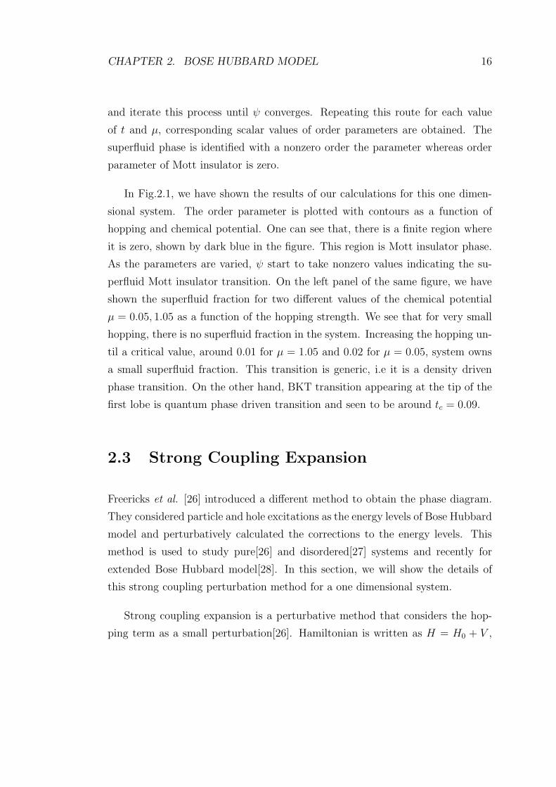
Figure 2.1: The order parameter calculated from self consistent meanfield ap-proximation as a function of chemical potential µ and hopping t is shown on theleft. The superfluid fraction as hopping in increased is shown on the right for twodifferent chemical potentials.
Hubbard model is obtained by Sheshadri et al. by use of this numerical mean-
field approximation. To show this method, we use one dimensional Bose Hub-
bard Hamiltonian. There are two nearest neighbors of each site under periodic
boundary conditions. Thus making the decoupling shown in Eq.(2.4) an effective
Hamiltonian valid for each site can be obtained as
Heffi = −t
[
2ψai + 2ψa†i − 2|ψ|2]
+1
2ni(ni − 1) − µni (2.5)
where ψ is a constant for order parameter. Note that, in general ψ may be
complex but we have taken it to be real for this specific case. The idea is the
following: For some fixed value of t and µ, we find a maximum occupation number
nmax for the Hamiltonian in Eq.(2.5) so that the ground state energy of the
effective Hamiltonian Heffi is the same for its representations in the truncated
basises nmax and nmax+1. Upon finding the maximum dimension of the truncated
basis (nmax) we solve Eq.(2.5) to find its lowest eigenvalue and corresponding
eigenvector. Let this eigenvector be |G〉, which is the ground state of effective
Hamiltonian. We substitute the following for order parameter
ψ = 〈G|a†i |G〉 (2.6)
CHAPTER 2. BOSE HUBBARD MODEL 16
and iterate this process until ψ converges. Repeating this route for each value
of t and µ, corresponding scalar values of order parameters are obtained. The
superfluid phase is identified with a nonzero order the parameter whereas order
parameter of Mott insulator is zero.
In Fig.2.1, we have shown the results of our calculations for this one dimen-
sional system. The order parameter is plotted with contours as a function of
hopping and chemical potential. One can see that, there is a finite region where
it is zero, shown by dark blue in the figure. This region is Mott insulator phase.
As the parameters are varied, ψ start to take nonzero values indicating the su-
perfluid Mott insulator transition. On the left panel of the same figure, we have
shown the superfluid fraction for two different values of the chemical potential
µ = 0.05, 1.05 as a function of the hopping strength. We see that for very small
hopping, there is no superfluid fraction in the system. Increasing the hopping un-
til a critical value, around 0.01 for µ = 1.05 and 0.02 for µ = 0.05, system owns
a small superfluid fraction. This transition is generic, i.e it is a density driven
phase transition. On the other hand, BKT transition appearing at the tip of the
first lobe is quantum phase driven transition and seen to be around tc = 0.09.
2.3 Strong Coupling Expansion
Freericks et al. [26] introduced a different method to obtain the phase diagram.
They considered particle and hole excitations as the energy levels of Bose Hubbard
model and perturbatively calculated the corrections to the energy levels. This
method is used to study pure[26] and disordered[27] systems and recently for
extended Bose Hubbard model[28]. In this section, we will show the details of
this strong coupling perturbation method for a one dimensional system.
Strong coupling expansion is a perturbative method that considers the hop-
ping term as a small perturbation[26]. Hamiltonian is written as H = H0 + V ,
CHAPTER 2. BOSE HUBBARD MODEL 17
where
H0 =1
2
∑
i
ni(ni − 1) − µ∑
i
ni
V = −∑
〈i,j〉
tija†iaj (2.7)
and U is taken to be one. Rayleigh-Schrodinger perturbation expression for the
energy up to second order can be written in its well known form,
Ek = E(0)k + E
(1)k + E
(2)k + . . .
= E(0)k + 〈Ψ(0)
k |V |Ψ(0)k 〉 +
∑
i6=k
|〈Ψ(0)k |V |Ψ(0)
i 〉|2E0k − E0
i
+ . . . (2.8)
where k is the state label that the correction will be done and |Ψ(0)k 〉 is the wave
function of this state. In the case of degeneracy, matrix representation of the
perturbation in the degenerate subspace is calculated and |Ψk〉 is chosen as the
ground state of this matrix. Exclusion of the state k in the sum turns out to
be exclusion of all states in the degenerate set, i.e i 6= k, for all k ∈ D, D is
the degenerate set. In the following we will show the calculation of perturbation
series up to second order for one dimensional Hubbard model to demonstare the
method.
Mott insulator state is characterized by a finite nonzero gap as mentioned
earlier. Gap is defined as the energy difference between two states; one with n0
particles in each lattice site and the other with a defect (one extra particle or
hole in one of the lattice sites). Let energies be shown by Em, Ep and Eh for
n0 particles per site, one extra particle and one extra hole respectively. Thus
Ep − Eh and Em − Eh will be nonzero at Mott insulator state. The place where
these gaps vanish will give the boundary of the Mott insulator state. In zeroth
order, atomic limit, the particle and hole excitation gaps can be written as
E(0)p −E(0)
m = E(n0 + 1) − E(n0) = n0 − µp
E(0)m −E
(0)h = E(n0) −E(n0 − 1) = (n0 − 1) − µh (2.9)
where E(n0) = n0(n0 − 1)/2 − µn0 is the single site energy. It can be seen
that, even in the atomic limit where hopping is not allowed, system can be in

CHAPTER 2. BOSE HUBBARD MODEL 18
the superfluid phase for µ = n0 or µ = n0 − 1 (at zero temperature). In the
following the energies of Mott and defect (particle and hole) states are calculated
perturbatively for nonzero hopping.
Mott State
In Mott state, all of the particle are localized and there are exactly n0 perticles
at each site. To the zeroth order, ground state of the system can be written as
|Ψ(0)M 〉 =
L∏
k=1
(a†k)n0
√n0!
|vac〉 (2.10)
where L is the number of lattice sites. The first order correction can be calculated
from Eq.(2.8) as E(0)M = 〈Ψ(0)
M |V |Ψ(0)M 〉 = 0, because 〈Ψ(0)
M |a†iaj |Ψ(0)M 〉 will be zero
for all i 6= j. The second order terms requires the calculation of matrix elements
〈Ψ(0)M |V |Ψ(0)
k 〉, where |Ψ(0)k 〉 is the set of all eigenvectors except the Mott state.
Explicit form of this term can be written as
〈Ψ(0)M |V |Ψ(0)
k 〉 = −∑
ij
tij〈Ψ(0)M |a†iaj |Ψ
(0)k 〉. (2.11)
The elements of the sum will be nonzero only for the eigenvectors of the form
|Ψ(0)k 〉 =
a†iaj√
n0(n0 + 1)|Ψ(0)
M 〉
where it is written in normalized form and i 6= j since otherwise it would be the
Mott state wave function. Also, i and j have to be nearest neighbors. For a one
dimensional model there are N such states. Matrix element for a particular such
state is found from the above wave function as 〈Ψ(0)M |V |Ψ(0)
k 〉 = −t√
n0(n0 + 1).
Energy difference between this state and the Mott state can be calculated by
considering that there are one extra particle and one extra hole in this state.
Thus the energy difference can be found as E(0)k − E
(0)M = −1. Using these
calculations, the second order correction is found from Eq.(2.8). The energy of
the Mott state up to second order is found as,
EM = E(0)M − 2Nt2n0(n0 + 1) +O(t3). (2.12)

CHAPTER 2. BOSE HUBBARD MODEL 19
Defect States
Correction to the defect states will be calculated in a similar manner. However
there is an important difference from the Mott state calculations: ground state of
the defects are N-fold degenerate, where N is the number of lattice sites. Because
an extra particle or hole can be placed N different places on the lattice each
having the same energy. Thus, we will use degenerate perturbation theory for
the first order correction. General normalized eigenvectors in this degenerate set
can be written as
|Ψ(0)P,i〉 =
a†i√n0 + 1
|Ψ(0)M 〉, |Ψ(0)
H,i〉 =ai√n0
|Ψ(0)M 〉 (2.13)
where P and H stand for particle and hole respectively and i runs from 1 to N.
Let us first consider the correction to the particle state. Construction of the
matrix representation of the perturbation in this degenerate set will be done by
using Vi′i = 〈Ψ(0)P,i′|V |Ψ(0)
P,i〉, which gives
Vi′i = −(n0 + 1)ti′i. (2.14)
Lowest eigenvalue of the hopping matrix can be calculated by Fourier trans-
forming the hopping term, which will give 2 in one dimension. Thus first order
correction to energy will be E(1)P = −2t(n0+1). Let the corresponding eigenvector
of this matrix V be shown by ~f . This will be used to find the correct form of the
ground state wave function as,
|Ψ(0)P 〉 =
∑
i
fia†i√n0 + 1
|Ψ(0)M 〉. (2.15)
Using this wavefunction in Eq.(2.8) the second order correction is found and the
total energy up to second is
EP = E(0)M +n0 −µp−2t(n0 +1)−2Nt2n0(n0 +1)+ t2n0(5n0 +4)−4t2n0(n0 +1).
(2.16)
Making the similar calculations for extra hole state, energy up to second order
can be found as
EH = E(0)M +µh−(n0−1)−2tn0−2Nt2n0(n0+1)+t2(n0+1)(5n0+1)−4t2n0(n0+1).
(2.17)

CHAPTER 2. BOSE HUBBARD MODEL 20
0 0.05 0.1 0.15 0.2 0.250
0.5
1
1.5
2
t
µ
Figure 2.2: Phase diagram of one dimensional Bose Hubbard Model calculatedfrom strong coupling perturbation up to second order.
Boundaries of the Mott insulator region will be found by solving EP − EM = 0
for µp, and EM − EH = 0 for µh. µp and µh give upper and lower boundaries
respectively. They are found to be
µp = n0 − 2t(n0 + 1) + t2n20
µh = (n0 − 1) + 2n0t− t2(n0 + 1)2. (2.18)
In Fig.2.2, we plot the boundaries found in Eq.(2.18) for the first two lobes
n0 = 1 and n0 = 2. The critical point that the BKT transition takes place is seen
to be at tc = 0.2. Comparison with the mean field calculation gives inconsistent
results. However we have shown both methods to show the details of the methods.
The decoupling approximation employed in the meanfield theory fails especially
for low dimensional systems where correlations are more pronounced. On the
other hand, strong coupling expansion is very strong for one dimensional systems.
In the next chapter, we will show the exact shape of phase diagram by using
density matrix renormalization group theory. One can see the power of the strong
coupling expansion by looking at this section of thesis.

CHAPTER 2. BOSE HUBBARD MODEL 21
2.4 Rotation in Bose Hubbard Model
Inclusion of a rotation to Bose Hubbard model is done by Pierls substitution,
which is based on the analogy between the rotation and the magnetic field pre-
sented in Chapter 1. For a two dimensional optical lattice rotating around an axis
perpendicular to the plane, Hamiltonian in Bose Hubbard model can be written
as
H = −t∑
〈i,j〉
eiAija†iaj +U
2
∑
i
ni(ni − 1) − µ∑
i
ni (2.19)
where A is the vector potential that satisfies B = ∇×A. Single particle spectrum
of this model was first considered by Hofstadter[29], in the context of electrons in
magnetic field. The range of magnetic field he argued was so large that it did not
get much attention by that time. However, the effective magnetic field in rotating
Bose Hubbard model is quite successfull for creation of these strong fields.
The energy spectrum of Bose Hubbard model under magnetic field gives Hofs-
tadter butterfly, which is strongly related to the Landau levels[30]. Thus, rotating
optical lattices provides a possibility to realize the exotic quantum phases in the
the fast rotation limit[31]. There has been a bunch of proposals and treatments for
the realization and detection of these strongly correlated phases[32, 33, 34, 35, 36].
But these works are limited to exact diagonalization studies of a few number of
particles on a few lattice sites which are far from thermodynamic limit. However
they have promising results for the discovery of fractional quantum Hall states in
the optical lattice setups. Recently, a composite fermion theory adapted to rotat-
ing Hubbard model is used to show the overlap of groundstate wavefunction with
the Loughlin state[37]. Theoretical and numerical tools are quite limited for the
exploration of rotating Hubbard model. The strongest approaches are meanfield
theory and strong coupling expansion which are both applied to rotating model
in [38] and [39] to find the Mott phase boundary. Motivated by these works, we
will analyze a toy model, rotating two leg Hubbard ladder, within these methods
in the following chapters. Apart from all, we will use density matrix renormal-
ization group theory to study exact nature of this simple quasi-one dimensional
system.

Chapter 3
Density Matrix Renormalization
Group Theory
Study of strongly correlated systems is one of the most active research areas of
both theoretical and experimental condensed matter physics. Bose Einstein con-
densates, Fermi gases, spin chains, superconducting curprates, Josephson junc-
tion arrays, cold atoms in optical lattices and even the quantum entanglement
can be given as examples of strongly correlated systems. Models of these systems
like Bose Hubbard model, Heisenberg spin Hamiltonian or t-J model contain the
key properties that display rich physical phenomena such as Mott transition,
spin gap, superconductivity etc. Yet, the solutions of these systems are difficult.
Analytical treatments are quite inadequate for the observation of important tran-
sitions. For example, mean field theory does not include the effect of correlations
whereas the perturbative approaches have limited range of validity due to the
strength of correlations. This makes computer simulations indispensable tools
for the exploration of strongly correlated systems.
On the other hand, numerical solution of those systems is not an easy job,
either. Exponential growth of the total Hilbert space dimension with increasing
lattice size makes it impossible to treat systems properly even for the strongest
computers today. Consider, for example, spin-1/2 antiferromagnetic Heisenberg
22

CHAPTER 3. DENSITY MATRIX RENORMALIZATION GROUP 23
chain, in which each individual site has a two dimensional Hilbert space. Hilbert
space grows as 2N with the number of lattice sites N which makes it very difficult
to simulate above a dozen of lattice sites.
Density Matrix Renormalization Group Theory (DMRG), developed by S.R.
White[40, 41, 42] as an extension of Wilson’s numerical renormalization group
method[43], is one of the strongest numerical approaches for the study of strongly
correlated quantum lattice models in one dimension. It systematically reduces
the dimension of the total Hilbert space by use of density matrices. Since its
invention it has been applied to a variety of lattice systems[44]. It is regarded
as giving the numerically exact solution but its main drawback is the absence
of implementation to higher than one dimensional systems which is currently an
active research area[45].
3.1 Exact Diagonalization
To introduce the mechanism of DMRG, the exact diagonalization methods will
be mentioned briefly. In this method, one considers the full Hilbert space of the
system as the direct products of the Hilbert spaces of the constituent subsystems
and solves the resulting eigenvalue problem exactly. There is no approximation
involved, thus this method gives exact solution for all parameter values up to
machine precision.
Consider a lattice system, that has local sites each having a finite Hilbert space
hi with the dimension di. One can write the full Hilbert space of a two site system,
for example, as H2 = h1⊗h2 where ⊗ is the direct product or Kronecker product
and the dimension of the total Hilbert space becomes d1d2 = d2. Similarly a
three site system can be written as H3 = h1 ⊗ h2 ⊗ h3 where the dimension of
total Hilbert space becomes d1d2d3 = d3. In general for an N site system, the full
Hilbert space can be written as
HN = h1 ⊗ h2 ⊗ · · · ⊗ hN (3.1)
with the dimension being d1d2 . . . dN = dN . It is seen that Hilbert space grows

CHAPTER 3. DENSITY MATRIX RENORMALIZATION GROUP 24
exponentially with increasing the number of sites. This is the reason why exact
diagonalization method is not applicable to all problems. It is difficult to fig-
ure out the properties of a system in the thermodynamic limit by use of exact
diagonalization.
For the reduction of the matrices to be diagonalized, the symmetries of the
system should be used. Conservation of the total angular momentum along z-
direction in antiferromagnetic Heisenberg model or the total number of particles
in Bose Hubbard model can be given as examples for the symmetries that can be
used. Consider one dimensional Heisenberg spin model. The Hamiltonian of this
model is
H = −J∑
i
Si · Si+1. (3.2)
For a simple system of 6 sites, Hilbert space dimension is 26 = 64. On the other
hand we know that the ground state of the system will be in Sztotal = 0 state.
This reduces the dimension down to 20, which is much less than that of the total
space. Symmetries to be used change from system to system but exploitation of
them is crucial for all numerical methods. To do this, one needs to find a quantity
that commutes with the Hamiltonian so that the Hamiltonian can be written in
block diagonal form and matrices to be solved will be much smaller.
3.2 Density Matrix
Consider an arbitrary state ket |φ〉. We define an operator like P = |φ〉〈φ|, which
is a projection operator on to the defined vector. What is the matrix representa-
tion of this operator in a given basis? The matrix elements of the operator can
be written as Pij = 〈i|φ〉〈φ|j〉. Expanding the kets in a set of complete states
as |φ〉 =∑
i′ ci′|i′〉, one can arrive at the following simple form; Pij = cic∗j . For
the case i = j the interpretation of this expression is straightforward: it is the
probability that the system can be in a specific state i. The case i 6= j , which
will be clear soon, seems to be undefined from a quantum mechanical point of
view. This can be made further complicated by slightly modifying the projection
operator P as; P = A|φ1〉〈φ1|+B|φ2〉〈φ2| where |φ1〉 and |φ2〉 are some arbitrary

CHAPTER 3. DENSITY MATRIX RENORMALIZATION GROUP 25
state vectors, which may or may not be orthogonal to each other. Action of
this operator is interpreted as the projection to two different states with some
weights A and B. Expanding the kets in a complete basis, |φ1〉 =∑
i′ ci′|i′〉and |φ2〉 =
∑
i′ di′ |i′〉 , one can find the matrix representation of this operator
as Pij = Acic∗j + Bdid
∗j . It is important for the case i = j that other weighting
factors A and B are introduced in the formalism, apart from the usual quantum
mechanical probabilities |ci|2 and |di|2.
Density matrix is the most general description for a quantum mechanical
system[46]. Quantum mechanics is established on the solution of Schrodinger
equation which results with a set of complete eigenstates. Once this is done,
any state |Ψ〉, whether an eigenstate of the Hamiltonian or not, can be described
by those complete set of vectors. Whenever some physical quantity S is con-
cerned, expectation values can be found as 〈Ψ|S|Ψ〉. On the other hand, real
systems cannot be described by this formalism since they are completely random
ensembles[46]. A collection of silver atoms in an oven or a beam of unpolarized
light can be given as the examples of completely random ensembles or ”mixed
ensembles” in the language of density matrix. For the example of silver atoms,
%50 of the atoms are spin up and %50 of them is spin down. Once they pass
from a Stern-Gerlach apparatus, they split into two diverging beams which are
now ”pure ensembles”, in terms of the z-components of the spins alone.
In general, density operator can be defined as,
ρ =∑
i
wi|φi〉〈φi| (3.3)
where wi’s are the percentages in the above example that are the statistical
probabilities in an ensemble. Density matrix is the matrix representation of this
operator in a basis, which can be obtained as above (in a more general way) by
using |φi〉 =∑
k cik|k〉, which gives
ρkk′ =∑
i
wicik(c
ik′)
∗. (3.4)
Notice that both quantum mechanical and statistical probabilities are combined
in the formalism. This is the basic purpose of the density matrix. Note that

CHAPTER 3. DENSITY MATRIX RENORMALIZATION GROUP 26
Tr(ρ) = 1 and it can be shown that the expectation value of any operator A
can be obtained as 〈A〉 = Tr(ρA). By using maximization of Neumann entropy
defined as S = −Tr(ρ ln ρ), it can also be shown that the weighting factors wi
are e−βEi so that the form of the density matrix is ρ = e−βH/Z, where Z is the
partition function[2]. In the limit of low temperatures which means β → ∞, only
the ground state’s weight becomes unity and all others zero. This is essentially a
pure state as explained above. Thus at low temperature limit, density matrix is
defined to be
ρ = |Ψ0〉〈Ψ0| (3.5)
3.2.1 Reduced Density Matrix
Physical systems are in general composite systems. System and heat bath or
environment in statistical mechanics, two particles entangled in a Bell state can
be given as specific examples for our purpose. Quantum mechanics treats a part
of those composite systems independently and solves them as if the other part
does not exits. Or, the solution is done for the whole composite system so that
constituent parts lose their identity. Another very important concept related to
the density matrix is the concept of reduced density matrix [47], which remedies
this inconvenience. Consider a system composed of two parts as shown in Fig.3.1.
Let the state vectors be |i〉 and |j〉 of each part A and B, respectively. Then the
most general state of the total system can be written as
|Ψ〉 =∑
ij
Ψij |i〉|j〉 (3.6)
where Ψij is the expansion coefficient. Assume we have an operator that acts
only one part of the system and does nothing to the other part. Then what is the
expectation value of this operator in state |Ψ〉? Let this operator be SA, where

CHAPTER 3. DENSITY MATRIX RENORMALIZATION GROUP 27
superscript A tells that it only acts on subsystem A. It can be evaluated as
〈Ψ|SA|Ψ〉 =∑
ij
∑
i′j′
ΨijΨ∗i′j′〈j′|j〉〈i′|SA|i〉 (3.7)
=∑
iji′
ΨijΨ∗i′j〈i′|SA|i〉
=∑
ii′
SAii′
[
∑
j
ΨijΨ∗i′j
]
where the term in the parantesis is defined to be the reduced density matrix. It
can be shown that it is equal to ρ = TrB(|Ψ〉〈Ψ|), where TrB(. . . ) means that
the trace is taken over the states of the system B alone. Thus, the expectation
value of the operator is 〈SA〉 = Tr(ρASA). We can write the reduced density
matrices of the subsystems A and B as
ρAii′ = TrB(|Ψ〉〈Ψ|) =∑
j
ΨijΨ∗i′j
ρBjj′ = TrA(|Ψ〉〈Ψ|) =∑
i
ΨijΨ∗ij′. (3.8)
i=1,2,...,NA
A B
|i> |j>
Bj=1,2,...,N
Figure 3.1: Schematic representation of a system composed of two parts A andB. |i〉 and |j〉 are the complete sets of states that span each subsystem.
3.2.2 Density Matrix Truncation
Assume that two systems A and B are in contact and correlated so that it is not
possible to write a separable solution for the energy eigenstates. Let there be NA

CHAPTER 3. DENSITY MATRIX RENORMALIZATION GROUP 28
states in the system A and NB states in B and let us label those states by |i〉 and
|j〉, respectively, as shown in Fig.3.1. Then, the most general state of the total
system A and B can be written in terms of complete set of states |i〉 and |j〉 as
|Ψ〉 =
NA∑
i=1
NB∑
j=1
Ψij|i〉|j〉. (3.9)
We want to take M most relevant states from the NA states in A so that NA −M states will be swept out[44, 48]. We can write those M states of the form
|α〉 =∑NA
i=1 uαi|i〉 where α = 1, ...,M and the expansion coefficients uαi are to be
determined later. We want to choose the most important states of the system A
where ‘important’ refers to the minimization of the norm, |||Ψ〉 − |Ψ〉|| for
˜|Ψ〉 =M∑
α=1
NB∑
j=1
aαj |α〉|j〉. (3.10)
Assuming real coefficients in the expansions for simplicity, we have
|||Ψ〉 − |Ψ〉||2 = 1 − 2∑
ijα
Ψijaαjuαi +∑
αj
a2αj . (3.11)
Taking the derivative of the above norm with respect to the coefficients aαj and
equating to zero, one finds that aαj =∑
i Ψijuαi. Inserting this expression into
Eq.(3.11), one arrives at
|||Ψ〉 − |Ψ〉||2 = 1 −∑
ijαi′
ΨijΨi′juαiuαi′ (3.12)
= 1 −∑
ii′α
uαiρii′uαi′
= 1 −∑
α
〈α|ρ|α〉
where ρ is the density matrix of the form ρii′ =∑
j ΨijΨi′j . For Eq.(3.12) to be
minimum |α〉’s must be eigenvectors corresponding to the largest eigenvalues of
the density matrix ρ, by Rayleigh-Ritz principle[44].
Thus, we arrive at the following conclusion. Once we have a very large Hilbert
space, we can systematically reduce the dimension by looking at the density
matrix eigenvalues. In DMRG, system is enlarged to a higher dimension by
adding a site to it and then reduced back to the beginning with the density
matrix projections. This will be explained in detail in the next section.
CHAPTER 3. DENSITY MATRIX RENORMALIZATION GROUP 29
3.3 DMRG Algorithms
DMRG is a renormalization group method that uses density matrices for system-
atic reduction of extra degrees of freedom[40]. In the standart block renormal-
ization group, developed by Wilson[43], system size is doubled and states that
has the lowest energies are discarded at each iteration, beginning from a single
site. It is found that this method was unable to describe interacting systems
properly. For example, it had failed for the description of a single particle in
infinite well potential. White and Noach soon noticed that it was the boundary
conditions that has to be taken care of. They fixed the failures of the method
by defining different boundary conditions[49] which was soon generalized in the
density matrix renormalization group method.
A.
Left Block Right Block
B.
Enlarged Rigth BlockEnlarged Left Block
D.
New Left Block New Right Block
C.
Super Block
Figure 3.2: Infinite system algorithm.
We have mentioned how to enumerate the states of a system, according to their
significance, in the previous section. Thus we need to make such a construction
that, it must be composed of two parts, which might be called as system and
environment, respectively. In the language of DMRG this distinction is named
by system block and environment block. In literature, blocks are named by left
CHAPTER 3. DENSITY MATRIX RENORMALIZATION GROUP 30
block for the system and right block for the environment, because of the one
dimensional structure of the models. Determination of the system and environ-
ment blocks is different in two different DMRG algorithms; infinite system and
finite system algorithms. In the infinite system algorithm, system size is increased
until convergence is obtained whereas in the finite system algorithm system size
is fixed but the the convergence is obtained by so called sweeps which will be
discussed later. To obtain a high numerical accuracy, infinite system algorithm
is insufficient and one needs to perform the finite system algorithm[40, 41].
3.3.1 Infinite System Algorithm
In the infinite system algorithm, both left and right blocks are enlarged at each
step, beginning from a single site, until the convergence is obtained. This process
is illustrated in Fig.3.2. In the beginning, left and right blocks are represented by
M-by-M matrices. Let us show left and right blocks by BL(k,M) and BR(k,M),
respectively. In this notation k stands for the number of sites in the block and
M is the dimension of the block. Similarly we represent a single site with s(D),
where D is the dimension of the site. Initially, we have right and left blocks as
shown in Fig.3.2A. Now, we enlarge these blocks by adding sites as shown in
Fig.2B. We have the left enlarged block BL(k,M) ⊗ s(D) and the right enlarged
block s(D)⊗BR(k,M). The size of the matrices of the enlarged blocks increased
to MD×MD. At this step it is important to write the Hamiltonian and other rel-
evant operators in the basis of an operator that commutes with the Hamiltonian.
This provides a block diagonal form for the Hamiltonian. The next step is the for-
mation of superblock Hamiltonian [BL(k,M) ⊗ s(D)]⊗ [s(D) ⊗ BR(k,M)] which
is shown if Fig.3.2C. This Hamiltonian is represented by (M ×D)2-by-(M ×D)2
matrix which is the largest matrix size that will be used. Thus it is crucial
to employ symmetries in the formation of the superblock Hamiltonian. Then,
the superblock Hamiltonian is diagonalized to find the lowest energy eigenstate
with a sparse matrix diagonalization routine and the reduced density matrices
are formed from Eq.(3.8). After that eigenvalues and eigenvectors of the density
CHAPTER 3. DENSITY MATRIX RENORMALIZATION GROUP 31
matrix are found with a dense matrix diagonalization routine and then the eigen-
vectors corresponding to the lowest M eigenvalues are used for the formation of
the projection matrices OL and OR as;
OL = (~v1~v2 . . . ~vM)
OR = (~u1~u2 . . . ~uM) (3.13)
where vi’s and ui’s are the eigenvectors of the left and right block density matrices
corresponding to M largest eigenvalues. OL and OR areMD×M matrices. Using
these matices, enlarged left and right block can be reduced to the dimension at
the beginning by using;
BL(k + 1,M) → O†L [BL(k,M) ⊗ s(D)]OL (3.14)
BR(k + 1,M) → O†R [s(D) ⊗ BL(k,M)]OR.
This process is shown is Fig.3.2D. After this step, left and right blocks are up-
dated and will be used as new blocks for the next iteration. After one iteration,
the number of sites in a block is increased from k to k+1 which shows the linear
growth in DMRG unlike the exponential growth in Wilson’s standart renormaliza-
tion group theory. Infinite system algorithm can be summarized in the following
steps;
1. Having left and right blocks, form the left and right enlarged blocks. Note
that left and right blocks are single sites at the very beginning of the algo-
rithm.
2. Form the superblock Hamiltonian which is composed of right and left en-
larged blocks.
3. Find the ground state eigenvector of the superblock Hamiltonian using a
sparse matrix diagonalization routine. The corresponding eigenvalue found
here gives the total energy of the system.
4. Using Eq.(3.8), form the reduced density matrices of the left and right
halves of the system from the eigenvector found in the previous step.

CHAPTER 3. DENSITY MATRIX RENORMALIZATION GROUP 32
5. Find the eigenvalues and eigenvectors of the reduced density matrices with a
dense matrix diagonalization routine and form the truncation operators OL
and OR from the highest weighted M eigenvectors of the density matrices
as given in Eq.(3.13).
6. Using OL and OR, transform the left and right enlarged blocks and save the
transformed blocks as new left and right blocks.
7. Using new left and right blocks, start from step 1 until the desired system
size is reached.
The most difficult and time consuming part of the algorithm is the diago-
nalization of the superblock Hamiltonian to find its ground state. Thus it very
important to make use of the symmetries of the system. For example total spin
along z direction in an antiferromagnetic Heisenberg spin model commutes with
the Hamiltonian so that Hamiltonian can be written in block diagonal form as we
mentioned before. Thus it is easier to find the ground state of this section in the
block diagonal form of the superblock. Similarly, commutation of total number
operator with total Hamiltonian in Bose Hubbard model can be exploited in the
diagonalization. For the diagonalization, one must use sparse matrix diagonal-
ization routines such as Lanczos or Jacobi algorithms[50].
3.3.2 Finite System Algorithm
Finite system algorithm is used to find the ground state properties of finite sys-
tems up to extreme accuracy. The procedure of the infinite system algorithm is
efficient for the search of properties in the thermodynamic limit. On the other
hand, one may be interested in some finite system where infinite system algorithm
gives relatively poor results. The difference between the two algorithms is in the
formation of environment and system blocks. In the finite system algorithm one
uses infinite system algorithm until the desired system length is obtained. This
part of the finite system algorithm is called warm up. In this process blocks are
saved as matrices in every iteration of warm up. If the length of the system is

CHAPTER 3. DENSITY MATRIX RENORMALIZATION GROUP 33
L, we than have information of BL1 ,BL
2 ,. . . ,BLL/2 and BR
1 ,BR2 ,. . . ,BR
L/2 at the end
of warm up. After this point, the size of the superblock is kept fixed in further
iterations so that system block size is increased whereas environment block size
is decreased. For example, the next superblock diagonalization after warp up is
of the form BLL/2 ⊗ s⊗ s⊗BR
L/2−2 , where s represents the operators of single sites
in between the blocks as before. The increase of the system size and the decrease
of the environment size is done until the system size reaches L − 3. That is,
superblocks in the successive steps are
BLL/2 ⊗ s⊗ s⊗ BR
L/2−2
BLL/2+1 ⊗ s⊗ s⊗BR
L/2−3
BLL/2+2 ⊗ s⊗ s⊗BR
L/2−4
...
BLL−3 ⊗ s⊗ s⊗BR
1 .
The system is swept to the right until the right block reduces to a single site. At
each step the information for the right block is read from the disk which was saved
in the warm up and new blocks for the left half are saved to the disk. For example,
BL/2+3 is obtained from the previous iteration by the truncation O†[BLL/2+2 ⊗s]O
where O is the truncation operator obtained from the reduced density matrix of
the left block as given in Eq.(3.13). Note that this density matrix is obtained
from the diagonalization of the super block BLL/2+2 ⊗ s⊗ s⊗BR
L/2−4. When right
block is a single site, the roles of left and right blocks are exchanged and same
procedure is applied until left block becomes a single site. And finally, the roles
of blocks are switched back again and left block is increased whereas right block
is reduced until the symmetric configuration BLL/2−1 ⊗ s⊗ s⊗BR
L/2−1 is obtained.
This whole operation,
. going right until the right end
. turning back and going left until the left end
. turning back and going right until the symmetric configuration BLL/2−1 ⊗
s⊗ s⊗BRL/2−1

CHAPTER 3. DENSITY MATRIX RENORMALIZATION GROUP 34
is called a complete sweep. After each sweep, accuracy increases and generally
two or three sweeps are enough for the convergence.
3.4 Applications
3.4.1 Heisenberg Model
Heisenberg Spin model has been the first application of density matrix renormal-
ization group theory because of its well established literature[51]. White applied
DMRG to spin-1/2 and spin-1 model to illustrate the power of the method he
developed[40].
The Hamiltonian for a one dimensional spin chain with nearest neighbor in-
teractions is given by,
H = −J∑
i
~Si · ~Si+1 = −J∑
i
Sxi Sxi+1 + Syi S
yi+1 + Szi S
zi+1 (3.15)
where i is the site index, J < 0 for the antiferromagnetic model and J > 0 for the
ferromagnetic model. The spin operators satisfy the usual commutation relations,
[Sx, Sy] = iSz
~ is taken to be unity and x,y and z can be permuted in cyclic order. Commutator
of the total Hamiltonian with Sz at a random site can be calculated as
[H,Szk ] =∑
i
[Sxi Sxi+1, S
zk ] + [Syi S
yi+1, S
zk ] (3.16)
= −iSxk+1Syk − iSxk−1S
yk + iSxkS
yk+1 + iSxkS
yk−1.
Summing this commutator over all k values gives zero which implies the conser-
vation of the total angular momentum along z direction. That is, for SzT =∑
i Szi ,
[H,SzT ] = 0.
In a similar fashion, it can be shown that [H, ~S2] = 0. These are the symmetries of
the Hamiltonian which are extremely important in the implementation of DMRG.

CHAPTER 3. DENSITY MATRIX RENORMALIZATION GROUP 35
Note that the second symmetry is very difficult to use in DMRG[44] but we will
show the use of conservation of SzT in the following discussion.
Using the transformation S± = Sx ± iSy and taking J = −1 for simplicity,
the Hamiltonian is written as
H =∑
i
1
2
(
S+i S
−i+1 + S−
i S+i+1
)
+ Szi Szi+1. (3.17)
3.4.1.1 Spin-1/2 System
For spin-1/2 system, the operators in above Hamiltonian are given by (for ~ = 1),
S+ =
(
0 1
0 0
)
S− =
(
0 0
1 0
)
Sz =1
2
(
1 0
0 −1
)
.
Analytical solution of this system is available[52] as well as numerical solution via
the Quantum Monte Carlo methods which makes it a strong benchmark for the
implementation of any numerical method. In the following, we are going to show
the first iteration of the infinite system algorithm as in the reference [53] but we
will give results of each step as it appears on a computer (instead of analytical
results of Malvezzi) for a demonstration.
At the beginning left and right blocks are single sites. Thus we define the
Hamiltonian of the blocks as
HL = HR =
(
0 0
0 0
)
(3.18)
and other operators of the blocks are same as single site operators so that
S+L = S+
R = S+ and SzL = SzR = Sz. One can obtain S− operator for a block
by taking the Hermitian conjugate of S−, thus it is unnecessary to save them
separately. Apart from the operators included in the interaction term, we need
to keep matrices that give the total angular momentum (along z direction) of the
blocks, separately. They are equal to Sz at the beginning so we save them as
STL = STR = Sz. We can now start to follow the DMRG algorithm:

CHAPTER 3. DENSITY MATRIX RENORMALIZATION GROUP 36
1. Obtaining the left and right enlarged blocks:
HeL = HL ⊗ I + S+
L ⊗ S− + S−L ⊗ S+ + SzL ⊗ Sz
HeR = I ⊗HR + S+ ⊗ S−
R + S− ⊗ S+R + Sz ⊗ SzL
Other operators of the enlarged blocks are constructed as (STL )e = STL⊗I+IL⊗Sz,(S+
L )e = IL ⊗ S+ and (SzL)e = IL ⊗ Sz where I stands for identity. Right block
operators can be constructed similarly. To show the results of these operations,
matrix representation of them are given as
HeL =
1
4
1 0 0 0
0 −1 2 0
0 2 −1 0
0 0 0 1
, (STL )e =
−1 0 0 0
0 0 0 0
0 0 0 0
0 0 0 1
, (3.19)
(SzL)e =
1
2
1 0 0 0
0 1 0 0
0 0 −1 0
0 0 0 −1
, (S+L )e =
0 0 1 0
0 0 0 1
0 0 0 0
0 0 0 0
.
Similar operators can be written for the right block. Note that Hamiltonian com-
mutes with the total angular momentum matrix along the z direction which is
seen from the block diagonal structure of the Hamiltonian. Keeping the states in
accordance with the SzT provides this block structure in the further iterations as
well.
2. Construction of the superblock Hamiltonian:
Hsb = HeL ⊗ IeR + IeL ⊗He
R + (S+L )e ⊗ (S−
R )e + (S−L )e ⊗ (S+
R)e + (SzL)e ⊗ (SzR)e
The dimension of the superblock is dim(Hsb) = dim(HeL)× dim(He
R) = 16 which
is the largest matrix throughout the iteration. Also, it is the matrix of which we
need to find the ground state eigenvalue and eigenvector. Thus, it is necessary to
employ symmetries here. It is known that ground state of Heisenberg spin system
without magnetic field is in total spin-z zero symmetry sector of the Hamiltonian.

CHAPTER 3. DENSITY MATRIX RENORMALIZATION GROUP 37
The dimension of this sector is 6, much less than the total dimension of the
superblock 16. The superblock is found as (see [53] for details),
Hsb =1
4
1 0 0 0 2 0
0 −3 2 2 0 2
0 2 −1 2 0 0
0 2 0 −1 2 0
2 0 2 2 −3 0
0 2 0 0 0 1
. (3.20)
3. Finding the ground state of the superblock : The lowest eigenvalue of this
matrix, found by a sparse matrix diagonalization routine is E = −1.6160 and
corresponding eigenvector is
|Ψ〉 =
0.1494
−0.5577
0.4082
0.4082
−0.5577
0.1494
. (3.21)
The state found above is called target state. Additional target states can be
obtained here if necessary. For example exited states of the system here can be
found by construction superblock in other nonzero spin-z sections which will be
used later to show the energy gaps in the system.
4. Formation of the reduced density matrices: At this step the coefficients
Ψij in Eq.(3.9) can be written as NA ×NB matrix. Thus density matrices of the
left and right blocks can be written as ρL = ΨΨ† and ρR = (Ψ†Ψ)T , respectively.

CHAPTER 3. DENSITY MATRIX RENORMALIZATION GROUP 38
Using the state given above, left block density matrix becomes
ρL =
0.0223 0 0 0
0 0.4777 −0.4553 0
0 −0.4553 0.4777 0
0 0 0 0.0223
. (3.22)
5. Finding the eigenvalues and eigenvectors of the density matrix : They are
0 10 20 30 40 5010
−5
10−4
10−3
10−2
10−1
100
L
Eex
act−E
dmrg
0 10 20 30 40
10−10
10−8
10−6
10−4
10−2
100
Figure 3.3: Convergence of the energy to the exact value is shown in the left paneand the decay of eigenvalues of the density matrix is in the right panel for M=24states kept.
found to be 0.9330, 0.0223, 0.0223, 0.0223, respectively. The exponential decay
of the eigenvalues can be seen here. Lets say we want to reduce the dimesion of
the enlarged blocks to 2, then the transformation matrix is constructed from the
highest two eigenvectors of the density matrix as
OL =
0 0
−0.7071 −0.7071
0.7071 −0.7071
0 0
(3.23)
where columns are the eigenvectors of ρL.
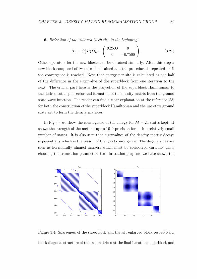
CHAPTER 3. DENSITY MATRIX RENORMALIZATION GROUP 39
6. Reduction of the enlarged block size to the beginning :
HL = O†LH
eLOL =
(
0.2500 0
0 −0.7500
)
. (3.24)
Other operators for the new blocks can be obtained similarly. After this step a
new block composed of two sites is obtained and the procedure is repeated until
the convergence is reached. Note that energy per site is calculated as one half
of the difference in the eigenvalue of the superblock from one iteration to the
next. The crucial part here is the projection of the superblock Hamiltonian to
the desired total spin sector and formation of the density matrix from the ground
state wave function. The reader can find a clear explanation at the reference [53]
for both the construction of the superblock Hamiltonian and the use of its ground
state ket to form the density matrices.
In Fig.3.3 we show the convergence of the energy for M = 24 states kept. It
shows the strength of the method up to 10−4 precision for such a relatively small
number of states. It is also seen that eigenvalues of the density matrix decays
exponentially which is the reason of the good convergence. The degeneracies are
seen as horizontally aligned markers which must be considered carefully while
choosing the truncation parameter. For illustration purposes we have shown the
0 100 200 300 400 500 600
0
100
200
300
400
500
600
Hsb
0 10 20 30 40
0
5
10
15
20
25
30
35
40
45
HL
Figure 3.4: Sparseness of the superblock and the left enlarged block respectively.
block diagonal structure of the two matrices at the final iteration; superblock and

CHAPTER 3. DENSITY MATRIX RENORMALIZATION GROUP 40
the left enlarged block. Superblock is the one corresponding to SzT = 0 symmetry
section and the off-block diagonal terms come from the interaction between the
left and right blocks. The block diagonal structure of the left enlarged block is
seen in the right panel; each block inside the matrix corresponds to a different
total spin.
3.4.1.2 Spin-1 System
Spin 1 system is modelled with the same Hamiltonian as in Eq.(3.17) where the
relevant operators have the following matrix representations
S+ =
0√
2 0
0 0√
2
0 0 0
S− =
0 0 0√2 0 0
0√
2 0
Sz =
1 0 0
0 0 0
0 0 −1
.
Haldane predicted that there must be a gap in the Heisenberg spin systems with
interger spin whereas no gap exists in the half interger systems[54]. There is
no analytical approach for the proof of this phenomenon and it was only shown
by other numerical methods such as quantum Monte Carlo method by the time
White developed the density matrix renormalization theory. He obtained the
energy gap for spin-1 system better than any other numerical method in his
work demonstrating the density matrix algorithm[40]. The algorithm for spin-1
system is a carbon copy of the procedure we demonstrated for spin-1/2 except
the definition of the local site operators. To check the reliability of our DMRG
code, we employed an exact diagonalization for some finite lattice, L = 8, and
calculated a few lowest lying states, as White did in his presentation of first
DMRG work[40]. Results of this comparison are given in Table 3.1. In Fig.3.5,
we have shown the convergence of the energy calculated from our code and the
eigenvalue spectrum of the density matrix. We have obtained ground state energy
per site as E/L = −1.40148 by taking M = 48 states and L = 100 sites in the
algorithm consistent with [42] up to 5 figures. Calculation of this energy took
about two minutes on a moderate PC. For comparison, we show the gap in spin-1
and spin-1/2 systems in Fig.3.5. Note that the gap is defined to be the energy
difference between the ground and first excited states for the spin-1/2 half system

CHAPTER 3. DENSITY MATRIX RENORMALIZATION GROUP 41
5 10 15 20 25 30 35−1.41
−1.4
−1.39
−1.38
−1.37
L
E
0 20 40 60 80 100 12010
−12
10−10
10−8
10−6
10−4
10−2
100
Figure 3.5: Energy per site as a function of system size is on the left for spin-1system with open boundary conditions. On the right decay of density matrixeigenvalues are shown
Table 3.1: Difference between energy calculated from exact diagonalization andthe energy of DMRG calculation for a finite size, L=8 site system.
M ST = 0 ST = 1 ST = 2
12 2.77 × 10⁻⁴ 1.42 × 10⁻³ 3.59 × 10⁻²
24 2.59 × 10⁻⁶ 2.01 × 10⁻⁵ 9.15 × 10⁻⁴
48 2.66 × 10⁻¹⁴ 1.24 × 10⁻¹⁴ 1.77 × 10⁻¹⁴
whereas it is the difference between SzT = 1 and SzT = 2 symmetry sectors which
correspond to the lowest two excited states for spin-1 system[51].
3.4.2 Bose-Hubbard Model
Bose Hubbard Hamiltonian is another model to which DMRG is applied. Al-
though the initial applications were done for the fermionic Hubbard model[55],

CHAPTER 3. DENSITY MATRIX RENORMALIZATION GROUP 42
0 0.02 0.04 0.06 0.08 0.1
0.05
0.1
0.15
0.2
1/L
E1 −E
0
0 0.05 0.1 0.15 0.2 0.250.4
0.41
0.42
0.43
0.44
0.45
100/L2
∆=E
2 −E1
y = 0.15*x + 0.41
dmrglinear fit
Figure 3.6: Haldane gap for spin-1/2 system as a function of inverse system sizeon the left and the one for spin-1 system as a function of inverse system sizesquared on the right. Gap is defined as the difference between ground state andthe first excited state ∆1/2 = E1 − E0 for spin-1/2 and difference between firstand second excited states ∆1 = E2 − E1 for spin-1.
we are going to present the results for the bosonic case. Bose Hubbard Hamilto-
nian with nearest neighbor hopping, in one dimension is given by,
H = −J∑
i
a†iai+1 + a†i+1ai +U
2
∑
i
ni(ni − 1) − µ∑
i
ni (3.25)
where ai and a†i are bosonic creation and annihilation operators defined on the
local sites which satisfy the commutation relation [ai, a†j ] = δij and ni = a†iai is the
number operator, J is the hopping strength, U is the onsite interaction strength
and µ is the chemical potential that controls the particle number fluctuation in
the grand canonical ensemble.
This model has been studied by density matrix renormalization extensively
and various properties has been explored. Mott-Superfluid-Bose glass phase dia-
gram of this model is obtained with and without additional nearest neighbor hop-
ping term by using both infinite and finite system algorithms[56, 57]. The model
with and without disorder has been explored by a different group via DMRG[58]
and phase diagrams are obtained for both extended Bose hubbard model[59] and
under harmonic confinement[60]. In the following, we give summary and details,

CHAPTER 3. DENSITY MATRIX RENORMALIZATION GROUP 43
when necessary, of some of these results and try to mention the basic methods
and approaches.
3.4.2.1 Ground State
Action of creation, annihilation and number operators on a state ket |n〉 can be
written as
a|n〉 =√n|n− 1〉, (3.26)
a†|n〉 =√n+ 1|n + 1〉,
n|n〉 = n|n〉.
Thus, one can write the infinite dimensional matrix representations of these op-
erators. In DMRG implementation, however, it is required to cut these infinite
dimensional operators at some point, say nmax, to use them in the algorithm. For
nmax = 4, they take the form
a =
0 1 0 0 0
0 0√
2 0 0
0 0 0√
3 0
0 0 0 0 2
0 0 0 0 0
, n =
0 0 0 0 0
0 1 0 0 0
0 0 2 0 0
0 0 0 3 0
0 0 0 0 4
. (3.27)
Having these finite matrices, its a straightforward application to implement usual
DMRG algorithm. To use the conservation of total number of particles, its pos-
sible to drop the term with chemical potential and work in canonical ensemble.
Hamiltonian for a single site will be hsite = n(n− I)/2 where I is identity matrix
and U is taken to be unity. Thus, it will be similar to the scheme presented be-
fore, except single site Hamiltonians are no longer zero. We follow the standart
recipe: enlargement of the blocks beginning from a single site, construction of the
superblock and finding the ground state to form the density matrices and finally
making truncations when necessary.
For the use of symmetries, it can be shown that [H,N ] = 0 where N is the
CHAPTER 3. DENSITY MATRIX RENORMALIZATION GROUP 44
total number operator given as
N =∑
i
ni (3.28)
Thus its the number operator that will be the basis for the construction of blocks
and enlarged blocks. To find the ground state of a system with known length, it
is necessary to set total number of particles. For example, to find ground state in
a Mott region, where there is one particle per site, we need to make projections
in the formation of superblock accordingly. For example, in the first iteration
projection will be made onto N = 4 sector where the superblock is composed of
4 sites . In the next iteration, where superblock this time has six sites, projection
will be made onto N = 6 sector, and so on. Energies of the defect states can be
found similarly. For instance, to find energy with one hole (particle), superblocks
will be projected onto L − 1 (L + 1) particles sector, where L is the number of
sites in the superblock. It is important to note that, accuracy of the results might
be poor for large differences between the length of the system (total number of
sites) and total number of particles. For the solution of one particle-hole defect
states, infinite system algorithm gives pretty good results, however it is necessary
to use the finite system algorithm for many particle-hole states.
In Fig.3.7, we have shown output of our DMRG code. Ground state energies
per particle have been plotted against the system size for Mott State, when
there is one particle per site, together with the additional one hole and one
particle states. The figure is plotted for two different values of the hopping
strength. For the small values of hopping strength, system is expected to be in
Mott insulator state that has a finite gap with particle hole excitations. As the
hopping strength increased, system undergoes a phase transition to the superfluid
phase characterized by gapless particle hole excitation. This transition is seen in
Fig.3.7 so that, the finite gap appearing for small J (left panel), disappears for a
large J (right panel).

CHAPTER 3. DENSITY MATRIX RENORMALIZATION GROUP 45
0 0.05 0.1 0.15 0.2 0.25−0.05
0
0.05
0.1
0.15
0.2
1/L
EJ=0.001
particleMottholelinear fit
0 0.05 0.1 0.15 0.2 0.25−1.8
−1.6
−1.4
−1.2J=1
1/L
E
particleMottholelinear fit
Figure 3.7: Ground state energies versus inverse system size of Bose Hubbardmodel for Mott state and particle-hole defect states for two different values ofhopping parameter,J = 0.001 (on left) and J = 1 (on right). Red straight linesare linear fits to DMRG points.
3.4.2.2 Superfluid-Mott Insulator Transition
The precision of the calculated energies with DMRG strongly depends on the
decay of density matrix eigenvalues. Carefull attention must be paid on the
determination of truncation parameter so that weighted majority of eigenvalues
of density matrix must be in the range of states that are kept at each iteration. For
the Bose Hubbard model treated here, correlations in the Mott insulator region
are small and the particles are well localized in sites if hopping strength is weak.
As the strength of hopping is increased, particles will loose their localization and
start to hop around. In this regime, the correlations are no more weak and the
number of states that are effective in the system increases. This can be seen
in Fig.3.8, where eigenvalue spectrum of the density matrix is shown for two
different hopping strengths. Thus the accuracy of the results decreases with the
same number of states kept while the hopping strength increases. One needs to
increase the number of states to obtain the same accuracy. In our calculations,
we calculated the error, ǫM = 1 −∑Mα=1 λα, to be order of 10−5 for J = 1 and
10−10 for J = 0.001 with M = 30 states kept.
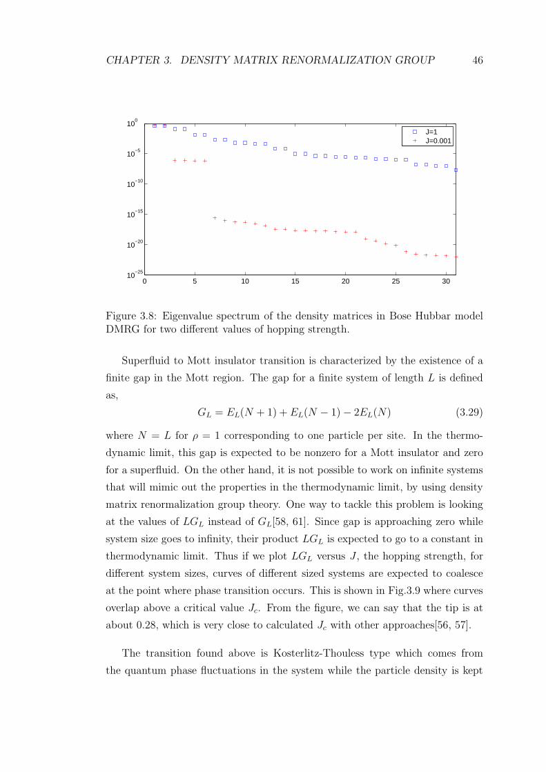
CHAPTER 3. DENSITY MATRIX RENORMALIZATION GROUP 46
0 5 10 15 20 25 3010
−25
10−20
10−15
10−10
10−5
100
J=1J=0.001
Figure 3.8: Eigenvalue spectrum of the density matrices in Bose Hubbar modelDMRG for two different values of hopping strength.
Superfluid to Mott insulator transition is characterized by the existence of a
finite gap in the Mott region. The gap for a finite system of length L is defined
as,
GL = EL(N + 1) + EL(N − 1) − 2EL(N) (3.29)
where N = L for ρ = 1 corresponding to one particle per site. In the thermo-
dynamic limit, this gap is expected to be nonzero for a Mott insulator and zero
for a superfluid. On the other hand, it is not possible to work on infinite systems
that will mimic out the properties in the thermodynamic limit, by using density
matrix renormalization group theory. One way to tackle this problem is looking
at the values of LGL instead of GL[58, 61]. Since gap is approaching zero while
system size goes to infinity, their product LGL is expected to go to a constant in
thermodynamic limit. Thus if we plot LGL versus J , the hopping strength, for
different system sizes, curves of different sized systems are expected to coalesce
at the point where phase transition occurs. This is shown in Fig.3.9 where curves
overlap above a critical value Jc. From the figure, we can say that the tip is at
about 0.28, which is very close to calculated Jc with other approaches[56, 57].
The transition found above is Kosterlitz-Thouless type which comes from
the quantum phase fluctuations in the system while the particle density is kept

CHAPTER 3. DENSITY MATRIX RENORMALIZATION GROUP 47
0 0.1 0.2 0.3 0.40
10
20
30
40
J
LGL
L=40L=30L=20
Figure 3.9: Gap multiplied by size vs hopping strength for different system sizeswith M = 30 states kept. Coalescence of curves for different lengths shows thetransition to superfluid. Transition is Kosterlitz-Thouless type.
constant. It is possible to obtain phase boundaries of Mott insulator region
coming from the density or number fluctuations in the system[56, 57]. Location
of this generic transition can be found by looking at the necessary energies to add
or subtract a particle from the system in Mott insulator, i.e
µpc = Ep −Em (3.30)
µhc = −Eh + Em
where µ is the chemical potential and Ep, Eh are the energies with one additional
particle, hole respectively and Em is the Mott insulator ground state energy. By
calculating these three energies the full phase boundary of the Mott Insulator
region can be obtained which is shown in Fig.10. It can be seen from the figure
that the tip of the insulator region do not close as J is increased, because the
transition is different at this point. They are expected to overlap in the thermo-
dynamic limit. This can be seen by running the same code for a larger system
size so that, the lines above and below will be closer to each other for larger L.
Combining the previous method shown in Fig.3.9, we can say that boundary at

CHAPTER 3. DENSITY MATRIX RENORMALIZATION GROUP 48
0 0.1 0.2 0.3 0.40
0.2
0.4
0.6
0.8
1
J
µ
MI
SF
SF
Figure 3.10: Phase diagram of one dimensional Bose hubbard model with onsiteinteraction. M = 30 states are kept in the dmrg iteration for a system of sizeL = 50. The BKT phase transition is not seen because of the method used whichis mentioned in the text.
this point is expected to be Jc = 0.28.
3.5 Conclusion
In this chapter, we summarize the steps of density matrix renormalization group
theory from the beginning. Very basic points of DMRG and details that were
difficult for us to understand are explained as we worked through the implemen-
tation of the algorithm. It is hoped that either the explanations given in the text
or the references given there will be helpful for a beginner. We tried to include all
the references that are used so that the reader can see them whenever necessary.
The basic theory of the DMRG, built on the density matrix formalism, is
presented and all steps required to write a program are given. To show the
mechanism and also the strength of the method, two different applications are
given; Heisenberg spin model and Bose Hubbard model. We skipped two very

CHAPTER 3. DENSITY MATRIX RENORMALIZATION GROUP 49
important parts: the observable expectations and the boundary conditions. The
method we have given is the so called open boundary consitions. Other boundary
conditions like periodic, soft or twisted is not mentioned. Reader might need to
see refences to work on these and a lot more topics that we did not mention here.
The most important problem of DMRG is that it can only be used for one
dimensional systems. If someone is working in one dimension or quasi-one dimen-
sion, DMRG is the most reliable method that can be used. It does not require
any information about the previous renormalization theories which makes it quite
accessible.

Chapter 4
Two Leg Bose Hubbard Model
In this chapter, two leg Bose Hubbard ladder under a uniform magnetic field is
studied. The model is introduced within the formalism of Bose Hubbard Hamil-
tonian and system parameters are defined below. Then different analytical and
numerical approaches are performed to study the model. In Section 4.1 nonin-
teracting particles on two legged ladder are studied and single particle spectrum
of the model is obtained. A critical magnetic field is found such that system
displays different properties above and below this critical value of the field. In
Section 4.2, interacting many particles on the two leg ladder are analyzed by use
of Gross Pitevskii approximation. An order parameter is defined and the result-
ing equation of motion is solved analytically to obtain the dispersion relation of
interacting many particles. In Section 4.3 superfluid to Mott insulator transition
is studied and Mott insulator phase boundary is obtained by using a variational
meanfield theory. In Section 4.4, the same phase diagram is obtained by strong
coupling perturbation and the results of the two different methods are compared.
In the last part, Section 4.5 and 4.6 exact behavior of the system is studied using
density matrix renormalization group (DMRG) theory .
50

CHAPTER 4. TWO LEG BOSE HUBBARD MODEL 51
System Hamiltonian is given by
H = − t∑
i
e−iαa†iai+1 + eiαb†ibi+1 + a†ibi +H.C. (4.1)
+U
2
∑
i
nai (nai − 1) + nbi(n
bi − 1) − µ
∑
i
nai + nbi
where ai (a†i ) are bosonic annihilation (creation) operators for upper leg, bi (b
†i ) are
bosonic annihilation (creation) operators for lower leg, nai = a†iai and nbi = b†ibi are
number operators, t is the hopping strength, U is the onsite interaction strength
and µ is the chemical potential. We are assuming a homogeneous system that
has up-down symmetry for zero magnetic field, so t, U and µ are taken identical
for each leg. The phase difference α gained by the hopping from position ri to rj
is calculated from
α =
∫ rj
ri
dr ·A(r) (4.2)
where and A is the vector potential satisfying ∇×A = B and B is the magnetic
field perpendicular to two leg plane. We use Landau gauge A = −Byx which
satisfies B = Bz. Note that this gauge does not brake the translational invariance
along x-direction. Thus the exponent in Eq.(4.1) is calculated from Eq.(4.2) as
α = πφ/φ0 where φ is the flux passing through each plaquette and φ0 = hc/e is
the flux quantum. For a two dimensional system, φ/φ0 is taken to be a rational
number p/q and the system is assumed to be q site periodic along y-direction
which partially fixes the symmetry broken by the gauge. Our system does not
require such a constraint so that α/π can be any real number between zero and
one.
4.1 Single Particle Spectrum
We first study the solution for non-interacting particles, U = 0, to obtain the
single particle spectrum. Single particle solution of the two dimensional Bose
Hubbard model under magnetic field ends up with a difference equation, called
Harper’s equation, that gives a fractal energy spectrum known as Hofstadter
butterfly. In the two leg ladder system, solution is much easier because of the

CHAPTER 4. TWO LEG BOSE HUBBARD MODEL 52
simpler symmetry of the system. Using the translational invariance along x-
direction, Fourier components of the field operators are written as,
aj =1√L
∑
k
akeikja, bj =
1√L
∑
k
bkeikja (4.3)
where L is the length of the system and Fourier components satisfy the commu-
tation [ak, a†k′] = δkk′ and [bk, b
†k′] = δkk′, all other commutators being zero. Using
these transformations in Eq.(4.1), the Hamiltonian is written in momentum space
as,
Hsp = −t∑
k
Aka†kak +Bkb
†kbk + a†kbk + b†kak (4.4)
where Ak = 2 cos (ka− πφ/φ0) and Bk = 2 cos (ka + πφ/φ0). One can define the
following Bogoliubov transformation for the diagonalization of the Hamiltonian
αk = cos θkak + sin θkbk, βk = − sin θkak + cos θkbk. (4.5)
It can be shown that this transformation is canonical and diagonalizes the Hamil-
tonian for θ = 12arctan ( 2
Ak−Bk). Thus the energy eigenvalues of this Hamiltonian
will have the form
ǫ1,2 = −Ak +Bk
2∓ 1
2
√
(Ak − Bk)2 + 4. (4.6)
In Fig.4.1, the dispersion relation in the first Brillouin zone is shown, for zero and
non-zero magnetic fields. It is seen that, as the strength of the field increases,
the energy band minimum in the dispersion shifts from k = 0 to two nonzero
k values which are degenerate and symmetric around the origin. Thus upon
increasing the magnetic field above a critical value, the system no longer bears
stationary solutions, but has travelling waves to the left or right. The critical value
of this magnetic field is found from the dispersion relation Eq.(4.6) by equating
the second derivative to zero with respect to k around k = 0. The critical value
of the field is αcr = cos−1[−√
17/4 + 1/4] which is numerically equal to 0.2148 or
0.7852 (0.7852 comes from the mirror symmetry of the energy spectrum around
α = 0.5). Above 0.2148 and and below 0.7852, k = 0 state changes from being
the energy minimum to a local energy maximum.
Another observation from the Fig.4.1 is that, for zero magnetic field, there
is no gap between the valence and the conduction band. On the other hand,

CHAPTER 4. TWO LEG BOSE HUBBARD MODEL 53
3−3 0−3
0
3
ka
E
ε1
ε2
−3 0 3−3
0
3
ka
E
ε1
ε2
Figure 4.1: Single particle band diagram two leg ladder under magnetic field.Left pane is plotted for α = 0 whereas right pane is for α = 0.4. The band gapbetween the conduction and the valance bands is zero for the left which is nonzerofor the right.
for α = 0.4 there is a finite band gap between these two energy bands. Thus,
introducing a magnetic field of a certain strength eventually gives rise to the
appearance of a gap in the spectrum. In Fig.4.2, we have plotted minima and
maxima of valence and conduction bands as a function of the magnetic field.
This plot can be regarded as ‘Hofstadter butterfly’ of the two legged quasi-one
dimensional system. From Fig.4.2 it is seen that the one and the largest gap
area of the spectrum is squeezed between α = 1/3 and α = 2/3 among the full
spectrum that is symmetric around α = 0.5.
4.2 Gross-Pitaevskii Approximation
For small values of the onsite interaction strength, the system is essentially in
the superfluid state, mostly governed by the hopping term in the Hamiltonian.
This enables us to define an order parameter which is the expectation value of
the field operator. Thus, assuming that the condensate is slowly varying over the
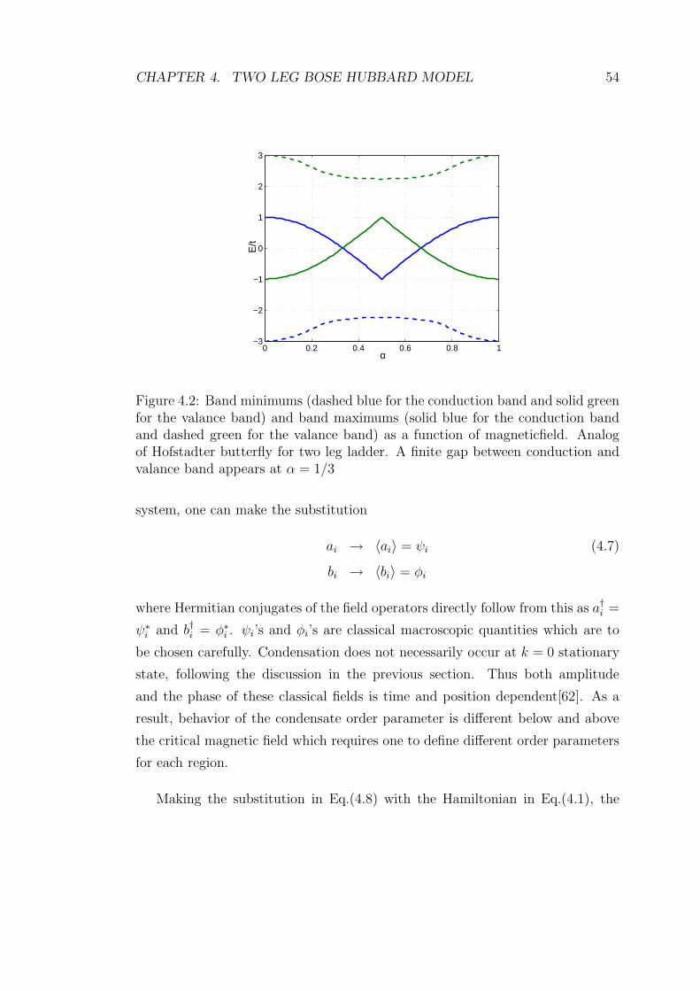
CHAPTER 4. TWO LEG BOSE HUBBARD MODEL 54
0 0.2 0.4 0.6 0.8 1−3
−2
−1
0
1
2
3
α
E/t
Figure 4.2: Band minimums (dashed blue for the conduction band and solid greenfor the valance band) and band maximums (solid blue for the conduction bandand dashed green for the valance band) as a function of magneticfield. Analogof Hofstadter butterfly for two leg ladder. A finite gap between conduction andvalance band appears at α = 1/3
system, one can make the substitution
ai → 〈ai〉 = ψi (4.7)
bi → 〈bi〉 = φi
where Hermitian conjugates of the field operators directly follow from this as a†i =
ψ∗i and b†i = φ∗
i . ψi’s and φi’s are classical macroscopic quantities which are to
be chosen carefully. Condensation does not necessarily occur at k = 0 stationary
state, following the discussion in the previous section. Thus both amplitude
and the phase of these classical fields is time and position dependent[62]. As a
result, behavior of the condensate order parameter is different below and above
the critical magnetic field which requires one to define different order parameters
for each region.
Making the substitution in Eq.(4.8) with the Hamiltonian in Eq.(4.1), the

CHAPTER 4. TWO LEG BOSE HUBBARD MODEL 55
following energy functional is obtained (take t = 1 for simplicity);
E[ψi, φi] = −∑
j
e−iαψ∗jψj+1 + eiαφ∗
jφj+1 + ψ∗jφj + c.c. (4.8)
+U
2
∑
j
ψ∗jψj(ψ
∗jψj − 1) + φ∗
jφj(φ∗jφj − 1) − µ
(
|ψi|2 + |φi|2)
.
Variations of the energy functional around the wavefunctions gives the dynamics
of the system, i.e. i~∂ψi
∂t= δE
δψi∗ and i~∂φi
∂t= δE
δφ∗i. These expressions give two
coupled equations,
i~∂ψj∂t
= −[
e−iαψj+1 + φj + eiαψj−1
]
+ U |ψj |2ψj −(
U
2+ µ
)
ψj (4.9)
i~∂φj∂t
= −[
eiαφj+1 + ψj + e−iαφj−1
]
+ U |φj |2φj −(
U
2+ µ
)
φj
which are nonlinear difference equations. These equations are nonlinear
Schodinger equations coupled to each other in discrete form, that is why we call
this section Gross-Pitaevskii approximation. Zeroth order terms ψj = φj =√n
will give the chemical potential as µ = −(2 cosα + 1) + 0.5U(2n− 1) which sat-
isfies the previously obtained dispersion relation in Eq.(4.6) for U = 0. For a
higher order approximation, small oscillations around this equilibrium value are
considered,
ψj =√n + Aei(k.rj−wt) +B∗e−i(k.rj−wt) (4.10)
φj =√n + Cei(k.rj−wt) +D∗e−i(k.rj−wt)
where A, B, C, D are small complex parameters and rj is a vector from the origin
to a lattice point and k being the reciprocal lattice vector. Inserting these wave-
functions into Eq.(4.10) and equating the exponents, the following determinant
is obtained for the existence of a nontrivial solution of the coefficients;
∣
∣
∣
∣
∣
∣
∣
∣
∣
∣
K + ~ω −Un 1 0
−Un L− ~ω 0 1
1 0 L+ ~ω −Un0 1 −Un K − ~ω
∣
∣
∣
∣
∣
∣
∣
∣
∣
∣
= 0

CHAPTER 4. TWO LEG BOSE HUBBARD MODEL 56
−3 0 30
2
4
6α=0
ka
E
−3 0 30
2
4
6
ka
E
Figure 4.3: Band diagrams for two leg ladder with onsite interactions calculatedfrom the Gross Pitaevskii approximation. Solid lines are for U = 0 and dottedlines are for U = 0.5. Left panel is for zero magnetic field and the right panel isfor α = 0.2
where K = 2cos(ka− α) − 2cos(α) − Un− 1 and L = 2cos(ka+ α) − 2cos(α) −Un − 1. Equating the determinant to zero, dispersion relation is obtained from
the solution of this matrix which is plotted in Fig.4.3.
In Fig.4.3, solid lines are for U = 0 and dotted lines are for U = 0.5. Non
interacting case is in agreement with the band diagram in Fig.4.1 apart from
an additive constant. The effect of interactions is to shift the band upward
for nonzero k whereas the band minimum persists on k = 0. Around k = 0,
interaction sharpens the band and provides a cusp like shape. On the other
hand, increase of the magnetic field, on the right panel, causes a smoother band
so that the linearity of the dispersion is lost. The expansion of the wave function
in Eq.(4.10) fails above the critical magnetic field, giving imaginary frequencies
which implies an unstable solution. We use this property to see the change of
the critical field with the interaction strength. In Fig.4.4, the change of the
critical magnetic field with the strength of the interaction is shown. It can be
seen that, U − αc relation is almost linear for small interaction strengths but it
saturates for strong interactions. Note that results of the strong onsite interaction
are not reliable because; firstly, the Gross Pitaevskii approximation is no more
valid in this region, secondly, attained magnetic field requires a wave function
different from the one in Eq.(4.10). Thus, we conclude that the critical magnetic

CHAPTER 4. TWO LEG BOSE HUBBARD MODEL 57
0 0.3 0.6 10.2
0.29
0.23
0.26
U
α c
0 25 500.3
0.4
0.5
Figure 4.4: Change of critical magnetic field with the increase of interactionstrength for low values of U , that is Un/t < 1. Plot is scaled with t = 1 andn = 1. In the limit U → 0, αc goes to the previously obtained value from thesingle particle solutions. Inset shows the behavior for large values of U , which isnot reliable because of strong interactions.
field increases linearly for weak interactions, that is for U < t/n. Increase of
interactions promotes solutions that are uniform through the lattice. That means,
to minimize the interaction energy, it is better to distribute particles uniformly
on the lattice. This makes wave functions proportional to√n more stable which
means that the onsite interaction increases the critical magnetic field strength.
4.3 Variational Mean Field Approach
In this section, we determine the Mott insulator phase boundary for different
values of the parameters t, µ and α. It is convenient to scale the Hamiltonian
in Eq.(4.1) with U = 1. In the perfect Mott insulator phase, each site has
a localized wavefunction and system is decoupled so that there are precisely n0
particles per site and the corresponding wavefunction is shown by |n0〉i in the Fock
basis. Allowing small variations around this equilibrium, the local wave functions
take the form ∆i|n0 − 1〉i + |n0〉i + ∆′i|n0 + 1〉i where ∆i and ∆′
i are variational
parameters to be determined. In general for a two dimensional Bose Hubbard

CHAPTER 4. TWO LEG BOSE HUBBARD MODEL 58
model, these parameters are assumed to be real since complex parameters are
expected to increase the energy[38] but for the two leg Bose Hubbard ladder, real
∆ assumption is found to give unbounded Mott insulator phase region. Thus,
the wave function is generalized to include complex values and the following
Gutzwiller ansatz is defined for local wave functions,
|G〉ka = ∆kaeiθk |n0 − 1〉ka + |n0〉ka + (∆k
a)′eiθk |n0 + 1〉ka (4.11)
|G〉kb = ∆kbeiθk |n0 − 1〉kb + |n0〉kb + (∆k
b )′eiθk |n0 + 1〉kb
where subscripts a and b stand for upper and lower legs respectively, superscripts
are site indices and θk is the additional variational parameter to be determined.
Having these local kets, the wave function for a rung becomes |Gr〉k = |G〉ka|G〉kband the total wavefunction of the system can be written as |Ψ〉 =
∏Nk |G〉ka|G〉kb .
This form of the wave function decouples the Hamiltonian in Eq.(4.1) and the
total energy of the system can be written as E = Nε, where ε is the variational
energy per a rung given by,
ε =〈Gr|H|Gr〉〈Gr|Gr〉
. (4.12)
Keeping terms up to second order in ∆, the following expression is obtained for
the energy per a rung
ε = − 2t cos (α + θ)[
∆2an0 + (∆′
a)2(n0 + 1) + 2
√
n0(n0 + 1)∆a∆′a
]
(4.13)
− 2t cos (α− θ)[
∆2bn0 + (∆′
b)2(n0 + 1) + 2
√
n0(n0 + 1)∆b∆′b
]
− 2t[
∆a∆bn0 + ∆′a∆
′b(n0 + 1) +
√
n0(n0 + 1)(∆a∆′b + ∆′
a∆b)]
+[
(1 − n0)(∆2a + ∆2
b) + n0(n0 − 1) + n0((∆′a)
2 + (∆′b)
2)]
+ µ[
(∆2a − (∆′
a)2) + (∆2
b − (∆′b)
2) − 2n0
]
where the site indices are not written for compactness. This energy is minimized
with respect to five variational parameters; four of them coming from ∆’s and
one from the phase θ. The first minimization is done on ∆’s. For the energy
in Eq.(4.14) to be a minimum, the Jacobian matrix should be positive definite (
all of the eigenvalues are positive). At the point where the determinant of the
Jacobian matrix is zero, the energy in Eq.(4.14) is no more a minimum of energy
which means that the system is not Mott insulator anymore. Jacobian matrix is

CHAPTER 4. TWO LEG BOSE HUBBARD MODEL 59
calculated as,
J = −2t
(
n0F√
n0(n0 + 1)F√
n0(n0 + 1)F (n0 + 1)F
)
(4.14)
+2
(
(1 − n+ µ)I 0
0 (n− µ)I
)
where I is 2 × 2 identity matrix and F has the same structure with the single
particle Hamiltonian in Eq.(4.4), which is
F =
(
2 cos (α + θ) 1
1 2 cos (α− θ)
)
. (4.15)
Positive definiteness of a matrix requires all eigenvalues to be positive. Thus the
minimum eigenvalue of the Jacobian matrix in Eq.(4.15) is found and equated to
zero to find the phase boundary of Mott insulator region. To find the eigenval-
ues, we use the following[38]; let λF and ~u be eigenvalues and eigenvectors of F
respectively, then one can apply an ansatz of the form
~v =
(
a~u
b~u
)
and solve the eigenvalue equation J~v = λ~v. The eigenvalues of Jacobian matrix
are found as
λ1,2 = 1 − tλF(2n0 + 1) (4.16)
±√
(1 − tλF(2n0 + 1))2 + 4tλF(µ+ 1) − 4(n0 − µ)(1 − n0 + µ).
Setting the smaller eigenvalue to zero and solving the corresponding equation for
t, the following relation is found for the boundary of Mott phase,
tc =(n0 − µ)(1 − n0 + µ)
(µ+ 1)λF
. (4.17)
Note that the eigenvalues λF in Eq.(4.17) are the same with energies in Eq.(4.6).
To plot the Mott phase boundary, we minimize the lowest eigenvalue with respect
to θ for each value of the magnetic field α.
In Fig.4.5, the result of the minimization is shown, which specifies a certain
region for Mott insulator phase. The complex variable θ plugged in the ansatz

CHAPTER 4. TWO LEG BOSE HUBBARD MODEL 60
0 0.2 0.4 0.6 0.8 1
0
0.2
0.4
0.6
0.8
1
α/π
θ/π
Figure 4.5: Mott phase boundary is shown on the left as a function of magneticfield strength and the chemical potential. Unlike two dimensional case, boundaryis perfectly smooth. On the right, result of the minimization of the energy withrespect to phase parameter θ in Eq.(4.12) is shown. It is seen that above thecritical magnetic field, the minimum energy ansatz bears complex amplitudes asin the case of single particle solution.
Eq.(4.12) follows the similar structure with that of the single particle solution;
above the critical magnetic field it takes nonzero values as shown on the right
panel of Fig.4.5. Our results are exact within mean field theory. On the other
hand, the meanfield theory applied to our system is not expected to give good re-
sults. This approach essentially decouples the hopping term in Eq.(4.1) and gives
it a mean field behavior. This decoupling is bad for low dimensions, especially for
one dimensional systems since correlations are more dominant in 1D relative to
two and three dimensions. Thus, this calculation is not expected to give accurate
results. The determination of the tip of the Mott lobe where BKT(Berezinskii,
Kosterlitz, Thouless) transition takes place and the calculation of the shape of
the Mott insulating region around this point is not reliable. On the other hand,
a rough sketch of the topology of the Mott insulator region is obtained within
this method. Additionally, for small values of the hopping strength, where the
correlations are diminished, the results are expected to be reliable.

CHAPTER 4. TWO LEG BOSE HUBBARD MODEL 61
...
...
...
1
2 4
3
6
5
N
N−1
Figure 4.6: Labelling of sites in two leg ladder for the calculation of strong cou-pling expansion
4.4 Strong Coupling Expansion
In the strong coupling perturbative expansion, the hopping term is taken to be
weak and considered as a perturbation. The Mott insulator state is character-
ized by a finite gap for particle-hole excitations whereas this gap vanishes for the
superfluid phase[18]. Thus if the energies of a system with n0 particles per site
(called Mott state) and a system with one additional defect (particle or hole) are
calculated, the difference between these two energies vanishes at the boundary of
Mott insulator phase. Then the solution of the equation, the difference of the two
energies be zero, with respect to chemical potential µ will give phase boundary
at the particle sector which is shown by µp. In a similar manner, phase bound-
ary of the hole sector, µh, can be obtained from the equation where the energy
difference of the Mott phase from one additional hole state becomes zero. In
the strong coupling expansion, energies of each of these three states (Mott state,
additional particle state and additional hole state) are calculated perturbatively.
This method has been used for systems with different dimensions[26, 27] and for
a two dimensional system under magnetic field[39].
To perform strong coupling expansion, it is convenient to write the Hamilto-
nian Eq.(4.1), in the following form,
H = −∑
ij
Tija†iaj +
1
2
∑
i
ni(ni − 1) − µ∑
i
ni (4.18)
where U is taken to be 1 and Tij is the hopping matrix, which is

CHAPTER 4. TWO LEG BOSE HUBBARD MODEL 62
T = t
A B 0 . . . 0 B†
B† A B 0. . . 0
0 B† A B. . .
......
.... . .
. . .. . . 0
0 . . . 0 B† A B
B 0 . . . 0 B† A
. (4.19)
A and B are 2 × 2 matrices of the form
A =
(
0 1
1 0
)
B =
(
e−iα 0
0 eiα
)
(4.20)
and α is the same parameter as before. It can be seen that, with the appropriate
labeling of sites as in Fig.4.6, this Hamiltonian is identical to the Hamiltonian in
Eq.(4.1) where the upper leg was distinguised from the lower one. This form of
Hamiltonian makes it easier to do perturbative calculations by considering the
hopping Tij as a general matrix which is real and symmetric.
We have performed strong coupling perturbation up to second order in our
calculations. The energies of Mott state EM , additional particle state EP and
additional hole state EH are found to be (up to second order)
EM = E0M − 3Nt2n0(n0 + 1) (4.21)
EP = E0P − (n0 + 1)λT − 3Nt2n0(n0 + 1) − n0(n0 + 1)λ2
T +3
2n0(5n0 + 4)t2
EH = E0H − n0λT − 3Nt2n0(n0 + 1) − n0(n0 + 1)λ2
T +3
2(n0 + 1)(5n0 + 1)t2
where λT is the lowest eigenvalue of the hopping matrix T and N is the number
of lattice sites which is always even in the two leg ladder. Zeroth order energies
are E0M = N(n0(n0−1)/2−µn0), E
0P = E0
M +n0−µ and E0H = E0
M−(n0−1)+µ.
A warning comes from first order corrections to EP and EH . Ground states of
these two systems (one additional hole-particle) are N-fold degenerate. In the first
order, these degeneracies do not split if the magnetic field is above the critical
field αc, which is expected because single particle solution give two degenerate
energies above αc as shown in Fig.4.6. On the other hand, matrix elements of
the perturbation, the hopping term, among those two degenerate kets do not

CHAPTER 4. TWO LEG BOSE HUBBARD MODEL 63
0 0.05 0.1 0.15 0.2 0.25 0.30
0.2
0.4
0.6
0.8
1
t
µ
00.5
1
α=0
α=0.2
α=0.4
0 0.2 0.4 0.6 0.8 1
0.1
0.2
0.3
0.4
α/π
t c
Figure 4.7: Phase diagram of two leg ladder, shown on the left, from strongcoupling perturbation theory for magnetic fields α = 0, α = 0.2 and α = 0.4compared with the results of meanfield calculation (dotted thin lines). Aboveα = 0.43 lines of µP and µH does not cross and higher oder perturbation isrequired. On the left the tip of the Mott region is shown as a function of field.Thin line after α = 0.43 is spline interpolant.
have any off-diagonal elements. This enables us to apply standart second order
perturbation safely as if the degeneracy is splitted in the first order[46]. Solving
the equations EP − EM = 0 and EM − EH = 0 for the chemical potentials µ
separately, the phase boundary of the particle and hole sector are obtained as,
µP = n0 − (n0 + 1)λT − n0(n0 + 1)λ2T +
3
2n0(5n0 + 4)t2 (4.22)
µH = (n0 − 1) + n0λT + n0(n0 + 1)λ2T − 3
2(n0 + 1)(5n0 + 1)t2.
Dependence of this form to the magnetic field comes indirectly from the eigenvalue
λT. To get a direct dependence on the field, higher order terms are required. An
interesting observation is that our results are similar to the results of Ref.[39] up
to second order if the number of nearest neighbors is taken 3, i.e z = 3. However
this is not guaranteed for higher order expansions since the flux attained should
be considered by additional particles and holes (see [26, 39] for details). The
eigenvalue spectrum of the T matrix is already shown in Fig.4.2. Dependence of
the minimum eigenvalue to the magnetic field is the dotted blue line in that figure.
It is seen that the spectrum has no cusp unlike the results in two dimension[39].

CHAPTER 4. TWO LEG BOSE HUBBARD MODEL 64
Results of strong coupling expansion in 1D are shown to be in very good
agreement with the numerically exact solutions[56, 57]. Thus, though we make
perturbation up to only second order, they are expected to be reliable for our
quasi-one dimensional system. In Fig.4.7 we have shown the results of our cal-
culation. It can be seen that, increase of the magnetic field, increases the Mott
insulating region. After some value of the magnetic field, reenterent behavior
to the Mott phase appears, as it is seen for α = 0.4 on the left panel. After
about the point α = 0.43 curves of particle and hole sector intersects at such a
large value of magnetic field that the second order perturbation fails to obtain
it and the two curves in Eq.(4.22) do not cross each other. However, apart from
the cusplike dip that BKT transition takes place, the results are expected to
be trustable. We have shown the change of critical hopping strength that BKT
transition occurs as a function of magnetic field on the right panel. Above the
point where two curves do not cross any more, a spline interpolation is done in
that figure. In Fig.4.7, we have also shown the related sector from the results
of meanfield calculation with dotted thin line. It is seen that mean field results
can hardly describe the system properly. Besides, mean field theory is already
expected to be poor for one dimensional systems as we have pointed out. A final
remark is that, for strong magnetic field αc > 0.4 the phase diagram takes the
shape of the one dimensional case found in [56]. The reenterent phase behavior
found in one dimensional system appears with the increase of magnetic field for
two leg ladder. This reenterent behavior was not previously seen in the results of
strong coupling perturbation neither in one two and three dimensions nor in two
dimensional lattice under magnetic field ( in [26, 27, 39] perturbation was carried
out up to third order). Existence of this reentrant phase is reliable since our
system is essentially one dimensional where strong coupling approach performs
its best.
4.5 DMRG Calculations
Density Matrix Renormalization Group (DMRG) theory has proven to provide
numerically exact solutions of one dimensional lattice systems[40, 41]. DMRG
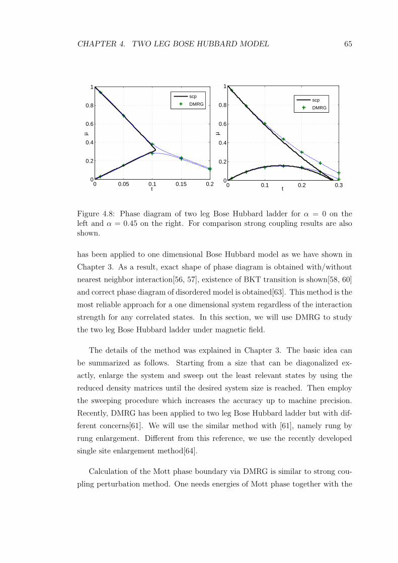
CHAPTER 4. TWO LEG BOSE HUBBARD MODEL 65
0 0.05 0.1 0.15 0.20
0.2
0.4
0.6
0.8
1
t
µ
scp
DMRG
0 0.1 0.2 0.30
0.2
0.4
0.6
0.8
1
t
µ
246
scp
DMRG
Figure 4.8: Phase diagram of two leg Bose Hubbard ladder for α = 0 on theleft and α = 0.45 on the right. For comparison strong coupling results are alsoshown.
has been applied to one dimensional Bose Hubbard model as we have shown in
Chapter 3. As a result, exact shape of phase diagram is obtained with/without
nearest neighbor interaction[56, 57], existence of BKT transition is shown[58, 60]
and correct phase diagram of disordered model is obtained[63]. This method is the
most reliable approach for a one dimensional system regardless of the interaction
strength for any correlated states. In this section, we will use DMRG to study
the two leg Bose Hubbard ladder under magnetic field.
The details of the method was explained in Chapter 3. The basic idea can
be summarized as follows. Starting from a size that can be diagonalized ex-
actly, enlarge the system and sweep out the least relevant states by using the
reduced density matrices until the desired system size is reached. Then employ
the sweeping procedure which increases the accuracy up to machine precision.
Recently, DMRG has been applied to two leg Bose Hubbard ladder but with dif-
ferent concerns[61]. We will use the similar method with [61], namely rung by
rung enlargement. Different from this reference, we use the recently developed
single site enlargement method[64].
Calculation of the Mott phase boundary via DMRG is similar to strong cou-
pling perturbation method. One needs energies of Mott phase together with the

CHAPTER 4. TWO LEG BOSE HUBBARD MODEL 66
additional particle and hole states to find the Mott insulator boundary. Thus,
the energies of particle and hole states are calculated as additional target states
in DMRG implementation[56]. Generally some limiting cases that are exactly
solvable are used to check the DMRG code. On the other hand, we have already
obtained the strong coupling expansion results for the system. There must be an
agreement between the two methods, especially for small hopping strength since
we make perturbation only up to second order. In Fig.4.8, one can see the good
agreement between the strong coupling result and DMRG. For larger values of
hopping, the strong coupling expansion fails to capture the exact behavior. An-
other point is the existence of reentrant phase even for zero magnetic field, which
is not seen by strong coupling. On the left panel we show the similar phase for
α = 0.45. Note that the strong coupling calculations give relatively poor results
above t ≈ 0.2 so that necessity of higher order terms becomes apparent. One
thing to be noted is that the tip of the Mott insulator region requires a special
treatment with DMRG. The two branches coming from particle and hole sector
intersect in the thermodynamic limit. However, DMRG takes finite systems far
from thermodynamic limit. There are several approaches (like consideration of
correlation length and extrapolation to Luttinger liquid correlation function in
[56] ) to remedy this situation which we don’t use because the tip of the lobe is
not our main concern (see Chapter 3).
4.6 Evidence of Strongly Correlated Phases
Up to now, we have performed various analytical calculations that can only work
around the Mott insulator phase. Theoretical approaches are quite limited for
the Bose Hubbard model under magnetic field, particularly for strong fields. This
is due to technical difficulties that stem from the strong correlations and high
number of degeneracies. Both strong coupling and mean field approaches work
on the region where those correlations are weak. On the other hand, the wealth
of the system lies underneath these ignored identities. Thus, the characterization
of the two dimensional Bose Hubbard model under strong magnetic field is very
important which is a popular research area. There has been several proposals

CHAPTER 4. TWO LEG BOSE HUBBARD MODEL 67
that try the connect these strongly correlated states either with the formation of
vortex lattice or with the incompressible quantum liquids found in quantum Hall
effect. Difficulty of the solution of the theoretical model makes it a hard task
to show the exact nature of the system. What can be done at best is an exact
diagonalization study of a small sized system with a few number of particles. But
these solutions are far from the thermodynamic limit and it has been found that
for strong magnetic fields the system does not resemble to be in some known
incompressible liquid phase[32, 37].
Strong coupling as well as mean field theory can predict quantum states near
Mott insulator phase as we have shown. They are valid when the total number
of particles is equal to the total number of lattice sites. On the other edge,
Gross Pitaevskii approximation assumes a uniform gas spread over the lattice to
reveal the dynamics of the system. Compared to these theoretical approaches,
DMRG gives a very wide range of applicability regardless of the particle number,
strength of the field and the interaction. One can calculate the ground state of the
system with any finite lattice size and any number of particles for all values of the
magnetic field and the interaction strength (as long as the eigenvalue spectrum
of the density matrix decays exponentially). The main drawback of DMRG is
that it can only be applied to one dimensional systems. The algorithm is difficult
to implement even for a few legged one dimensional systems. Another point is
the fact that DMRG works for finite sized systems which may be particularly
important for the properties in the thermodynamic limit. In this section we will
use DMRG to study the two leg Bose Hubbard model under magnetic field out
of the Mott insulator region.
We make DMRG calculations for hard core bosons in infinite U limit. Pro-
viding an easier implementation of the algorithm which also works fast, this limit
is particularly important for experimental realizations. Because the gaps are ex-
pected to be more prominent with strong interactions. With this approximation
each site is allowed to be empty or have only one boson so that maximum occu-
pation number nmax = 1 and the term with the onsite interaction in the Hamil-
tonian is removed. In this approximation, Bose Hubbard model is expected to be
mapped to spin-XXZ model, where ground state is at half filling[51]. We found

CHAPTER 4. TWO LEG BOSE HUBBARD MODEL 68
0 0.1 0.2 0.3 0.4 0.50
0.1
0.2
0.3
α/π
∆
Figure 4.9: Gap between ground state and two excited states for different mag-netic field. The gap between first excited state E1 − E0 is shown by green ’+’,whereas the one for E2 − E0 is shown by blue ’’. Thin lines are spline interpo-lation to data points. It is seen that around αc = 0.21 spectrum has a jump to acompletely different behavior.
that our system has a ground state at half filling not only for α = 0 but also
for nonzero α. In two distinct limits; all sites are empty and all sites are filled,
ground state energy is zero and minimum of the energy is always at half filling
which is in the middle of these two limits.
We obtain energies for different values of magnetic field, on the half filling par-
ticle sector of the superblock Hamiltonian. The energy gap between the ground
state and first two excited states is obtained and shown in Fig.4.9. From the fig-
ure, it can be seen that spectrum of the three lowest lying states changes abruptly
to a different pattern at αc = 0.21. This plot is symmetric around α = 0.5 so we
only show one half. The critical value found here is perfectly consistent with the
one found in single particle solution, which were equal to 0.2148 or 0.7852. Note
that spectrum is not smooth at α = 0.5 but has a cusp.
To get the energies at various fillings, we use the route proposed by Ramanan

CHAPTER 4. TWO LEG BOSE HUBBARD MODEL 69
0 0.167 0.5 0.835 1
0
0.04
0.08
0.12
n
∆
1/6 5/6
0 0.2 0.4 0.6 0.8 1
0
0.1
0.2
n
∆
1/5 4/5
0 0.25 0.5 0.75 1
0
0.1
0.2
0.3
0.4
n
∆
1/4 3/4
Figure 4.10: Energy gap defined in Eq.4.23 as a function of particle density forα = 1/3 in the first figure, 2/5 in the second and 1/2 in the third respectively.For each value of α, a different peak is seen in the energy gap where the peaks aresymmetric around 0.5. Apart from the dominant peaks at 1/5, 1/6 for α = 1/3,1/5, 4/5 for α = 2/5 and 1/4, 3/4 α = 1/2 and the persistent peak at 1/2, thereseem to be fluctuating non zero gap value for other fillings.

CHAPTER 4. TWO LEG BOSE HUBBARD MODEL 70
Table 4.1: Value of the filling factor defined in Eq.4.24 for different magneticfields shown in Fig.4.10
α n1 ν1 n2 ν2 n3 ν3
1/3 1/6 1/2 5/6 3/2 5/6 5/22/5 1/5 1/2 4/5 5/4 4/5 21/2 1/4 1/2 3/4 1 3/4 3/2
et al.[60] for a system of length L = 60 that has 2 × L = 120 sites. Beginning
from L = 4 and total number of particles N = 4 (since we know minimum energy
is at half filling for infinite U), we increase both the lattice length and the number
of particles up to where the total number of particles is, lets say, N = 10. After
that, the lattice length is increased while total number of particles held fixed at
10. Whenever lattice length reaches the desired length, L = 60, finite system
sweeps are used to get better energy. Next the system size is held fixed while
particle number is increased, by doing 5 sweeps for each particle number. Total
number of particles is increased up to N = 110. At the end, energies of systems
from N = 10 to N = 110 particles placed on 2 × L = 120 sites are obtained.
Ramanan et al. obtained the plateaus in the chemical potential versus density
plots and corresponding compressibilities by using this method. After that, the
gap formula defined by Cooper et al.[65] is used which has the form
∆ = N
[
E(N + 1)
N + 1+E(N − 1)
N − 1− 2
E(N)
N
]
(4.23)
which minimizes the finite size effects. This gap is shown for various values of
magnetic field in Fig.4.10. It is seen that the gap oscillates between zero and
nonzero values for low densities and becomes negative towards interger filling.
Apart from that, there are three dominant peaks one is always at 1/2 and the
other two change with different α. Magnitude of these changing peaks are also
seen to be getting smaller and smaller as the field approaches 1/2. It is interesting
to compare these peaks by defining the filling factor[66],
ν =n
f(4.24)
where n is particle density and f is vortex density defined as the phase attained
around a unit cell divided by 2π. In our model, it can be shown that 2πf = 2α so

CHAPTER 4. TWO LEG BOSE HUBBARD MODEL 71
that f = α/π. In Table 4.1, we have shown the values of filling factor by looking
at the peaks in Fig.4.10. One can see that various fillings are obtained as 1/2, 1,
5/4, 3/2, 5/2.
4.7 Conclusion
We have studied on the two leg Bose Hubbard ladder exposed to a strong magnetic
field within various theoretical approaches and implemented DMRG to study
the exact behavior of the system. It is found that system has two different
behaviors above and below the critical magnetic field. The shape of the Mott
insulator region is obtained within three different methods; variational meanfield
theory, strong coupling perturbation and DMRG. It is found that the shape
of the lobe is very consistent within DMRG and strong coupling whereas the
results of the meanfield theory is relatively poor. This was already expected
because mean field theory ignores the strong correlations that are particularly
important for low dimensional systems. Apart from the determination of the Mott
lobes, the system is found to display novel physical properties from the results of
single particle spectrum and Gross Pitaevskii approximation. We believe that this
toy model serves as an important tool for understanding the general properties
of the rotating optical lattices and the theoretical methods that are used most
frequently. In the last part of the chapter, we have worked on the characterization
of strongly correlated phases in the hard core limit. The system is found to display
incompressible liquid phases at various fillings depending on the field strength
where these states are completely different from the incompressible Mott insulator
state. Our work on the system for soft bosons (that is, different from the infinite
U limit) is in progress. This system is believed to be very rich for the exploration
of exotic quantum phases.

Bibliography
[1] F Dalfovo, S Giorgini, LP Pitaevskii, and S Stringari. Theory of Bose-
Einstein condensation in trapped gases. Reviews of Modern Physics,
71(3):463–512, Apr 1999.
[2] Kerson Huang. Statistical mechanics. Wiley, 1987.
[3] Wolfgang Ketterle. Nobel lecture: When atoms behave as waves: Bose-
einstein condensation and the atom laser. Reviews of Modern Physics,
74(4):1131+, November 2002.
[4] E. A. Cornell and C. E. Wieman. Nobel lecture: Bose-einstein condensation
in a dilute gas, the first 70 years and some recent experiments. Rev. Mod.
Phys., 74(3):875–893, Aug 2002.
[5] AJ Leggett. Bose-Einstein condensation in the alkali gases: Some funda-
mental concepts. Reviews of Modern Physics, 73(2):307–356, Apr 2001.
[6] V. I. Yukalov. Cold bosons in optical lattices. Laser Physics, 19(1):1–110,
Jan 2009.
[7] A. J. Leggett. Quantum liquids : Bose condensation and Cooper pairing in
condensed-matter systems. Oxford University Press, 2008.
[8] H. Smith C. J. Pethick. Bose-Einstein condensates in dilute atomic gases.
Cambridge University Press, 2002.
[9] Alexander L. Fetter. Rotating trapped bose-einstein condensates. Reviews
of Modern Physics, 81(2):647, 2009.
72

BIBLIOGRAPHY 73
[10] James F. Annet. Superconductivity, Superfluids and Condensates. Oxford
University Press, 2004.
[11] A. L. Fetter and J. D. Walecka. Quantum Theory of Many Particle Systems.
Dover Publications, 2003.
[12] TL Ho. Bose-Einstein condensates with large number of vortices. Physical
Review Letters, 87(6), Aug 6 2001.
[13] S Stock, B Battelier, V Bretin, Z Hadzibabic, and J Dalibard. Bose-Einstein
condensates in fast rotation. Laser Physics Letters, 2(6):275–284, Jun 2005.
[14] V. Schweikhard, I. Coddington, P. Engels, V. P. Mogendorff, and E. A.
Cornell. Rapidly rotating bose-einstein condensates in and near the lowest
landau level. Phys. Rev. Lett., 92(4):040404, Jan 2004.
[15] Vincent Bretin, Sabine Stock, Yannick Seurin, and Jean Dalibard. Fast
rotation of a bose-einstein condensate. Phys. Rev. Lett., 92(5):050403, Feb
2004.
[16] Rajiv Bhat, M. Kramer, J. Cooper, and M. J. Holland. Hall effects in bose-
einstein condensates in a rotating optical lattice. Physical Review A (Atomic,
Molecular, and Optical Physics), 76(4):043601, 2007.
[17] S. Tung, V. Schweikhard, and E. A. Cornell. Observation of vortex pinning
in bose-einstein condensates. Physical Review Letters, 97(24):240402, 2006.
[18] Matthew P. A. Fisher, Peter B. Weichman, G. Grinstein, and Daniel S.
Fisher. Boson localization and the superfluid-insulator transition. Phys.
Rev. B, 40(1):546–570, Jul 1989.
[19] D Jaksch, C Bruder, JI Cirac, CW Gardiner, and P Zoller. Cold bosonic
atoms in optical lattices. Physical Review Letters, 81(15):3108–3111, Oct 12
1998.
[20] D van Oosten, P van der Straten, and HTC Stoof. Quantum phases in an
optical lattice. Physical Review A, 63(5), May 2001.

BIBLIOGRAPHY 74
[21] M Greiner, O Mandel, T Esslinger, TW Hansch, and I Bloch. Quantum
phase transition from a superfluid to a Mott insulator in a gas of ultracold
atoms. Nature, 415(6867):39–44, Jan 3 2002.
[22] I Bloch. Ultracold quantum gases in optical lattices. Nature Physics, 1(1):23–
30, Oct 2005.
[23] Immanuel Bloch, Jean Dalibard, and Wilhelm Zwerger. Many-body physics
with ultracold gases. Reviews of Modern Physics, 80(3):885, 2008.
[24] C Bruder, R Fazio, and G Schon. The Bose-Hubbard model: from Josephson
junction arrays to optical lattices. Annalen Der Physik, 14(9-10):566–577,
Sep-Oct 2005.
[25] K Sheshadri, HR Krishnamurthy, R Pandit, and TV Ramakrishnan. Su-
perfluid and Insulating Phases in an Interacting-Boson Model - Mean-Field
Theory and the RPA. Europhysics Letters, 22(4):257–263, May 1 1993.
[26] JK Freericks and H Monien. Phase-Diagram of the Bose-Hubbard Model.
Europhysics Letters, 26(7):545–550, Jun 1 1994.
[27] J. K. Freericks and H. Monien. Strong-coupling expansions for the pure and
disordered bose-hubbard model. Phys. Rev. B, 53(5):2691–2700, Feb 1996.
[28] M. Iskin and J. K. Freericks. Strong-coupling perturbation theory for the
extended Bose-Hubbard model. Physical Review A, 79(5), May 2009.
[29] Douglas R. Hofstadter. Energy levels and wave functions of bloch electrons
in rational and irrational magnetic fields. Phys. Rev. B, 14(6):2239–2249,
Sep 1976.
[30] JG Analytis, SJ Blundell, and A Ardavan. Landau levels, molecular orbitals,
and the Hofstadter butterfly in finite systems. American Journal of Physics,
72(5):613–618, May 2004.
[31] Susanne Viefers. Quantum hall physics in rotating Bose-Einstein conden-
sates. Journal of Physics-Condensed Matter, 20(12), Mar 26 2008.
BIBLIOGRAPHY 75
[32] R Bhat, MJ Holland, and LD Carr. Bose-Einstein condensates in rotating
lattices. Physical Review Letters, 96(6), FEB 17 2006.
[33] RN Palmer and D Jaksch. High-field fractional quantum Hall effect in optical
lattices. Physical Review Letters, 96(18), May 12 2006.
[34] Rajiv Bhat, B. M. Peden, B. T. Seaman, M. Kramer, L. D. Carr, and M. J.
Holland. Quantized vortex states of strongly interacting bosons in a rotating
optical lattice. Physical Review A, 74(6), Dec 2006.
[35] Rajiv Bhat, M. Kraemer, J. Cooper, and M. J. Holland. Hall effects in Bose-
Einstein condensates in a rotating optical lattice. Physical Review A, 76(4),
Oct 2007.
[36] M. Hafezi, A. S. Sorensen, E. Demler, and M. D. Lukin. Fractional quantum
Hall effect in optical lattices. Physical Review A, 76(2), Aug 2007.
[37] Gunnar Moller and Nigel R. Cooper. Composite fermion theory for bosonic
atoms in optical lattices, 2009.
[38] R. O. Umucalilar and M. O. Oktel. Phase boundary of the boson Mott
insulator in a rotating optical lattice. Physical Review A, 76(5), Nov 2007.
[39] M. Niemeyer, J. K. Freericks, and H. Monien. Strong-coupling perturbation
theory for the two-dimensional bose-hubbard model in a magnetic field. Phys.
Rev. B, 60(4):2357–2362, Jul 1999.
[40] Steven R. White. Density matrix formulation for quantum renormalization
groups. Phys. Rev. Lett., 69(19):2863–2866, Nov 1992.
[41] Steven R. White. Density-matrix algorithms for quantum renormalization
groups. Phys. Rev. B, 48(14):10345–10356, Oct 1993.
[42] Steven R. White and David A. Huse. Numerical renormalization-group study
of low-lying eigenstates of the antiferromagnetic s=1 heisenberg chain. Phys.
Rev. B, 48(6):3844–3852, Aug 1993.
[43] KG Wilson. The renormalization and critical phenomena. Reviews Of Mod-
ern Physics, 55(3):583–600, 1983.

BIBLIOGRAPHY 76
[44] U. Schollwock. The density-matrix renormalization group. Rev. Mod. Phys.,
77(1):259–315, Apr 2005.
[45] N Shibata. Application of the density matrix renormalization group method
to finite temperatures and two-dimensional systems. Journal of Physics A-
Mathematical and General, 36(37):R381–R410, Sep 19 2003.
[46] J.J. Sakurai. Modern Quantum Mechanics. Addison-Wesley, revised edition,
1994.
[47] Richard Phillips Feynman. Statistical mechanics; a set of lectures / Ed. by
Jacob Shaham. Addison-Wesley, 1972.
[48] M. Kaulke I. Peschel, X. Wang and K. Hallberg (Eds.). Density-matrix
renormalization: a new numerical method in physics : lectures of a seminar
and workshop held at the Max-Planck-Institut fr Physik Komplexer Systeme,
Dresden, Germany, August 24th to September 18th, 1998. Springer Verlag,
1999.
[49] SR White and RM NOACK. Real space quantum-renormalization groups.
Physical Review Letters, 68(24):3487–3490, Jun 15 1992.
[50] RM Noack and SR Manmana. Diagonalization- and numerical
renormalization-group-based methods for interacting quantum systems. In
Avella, A and Mancini, F, editor, Lectures on the Physics of Highly Corre-
lated Electron Systems IX, volume 789 of AIP Conference Proceedings, pages
93–163, 2005. 9th Training Course in the Physics of Correlated Electron Sys-
tems and High-Tc Superconductors, Salerno, ITALY, OCT 04-15, 2004.
[51] I Affleck. Quantum spin chains and the Haldane gap. Journal of Physics-
Condensed Matter, 1(19):3047–3072, May 15 1989.
[52] Elliott Lieb, Theodore Schultz, and Daniel Mattis. Two soluble models of an
antiferromagnetic chain. Annals of Physics, 16(3):407–466, December 1961.
[53] AL Malvezzi. An introduction to numerical methods in low-dimensional
quantum systems. Brazilian Journal of Physics, 33(1):55–72, Mar 2003.

BIBLIOGRAPHY 77
[54] FDM Haldane. Continuum dynamics of the 10D Heisenberg anti-ferromagnet
- identification with the O(3) non-linear sigma-model. Physics Letters A,
93(9):464–468, 1983.
[55] R. M. Noack, S. R. White, and D. J. Scalapino. Correlations in a two-chain
hubbard model. Phys. Rev. Lett., 73(6):882–885, Aug 1994.
[56] TD Kuhner, SR White, and H Monien. One-dimensional Bose-Hubbard
model with nearest-neighbor interaction. Physical Review B, 61(18):12474–
12489, May 1 2000.
[57] TD Kuhner and H Monien. Phases of the one-dimensional Bose-Hubbard
model. Physical Review B, 58(22):14741–14744, Dec 1 1998.
[58] RV Pai, R Pandit, HR Krishnamurthy, and S Ramasesha. One-dimensional
disordered bosonic Hubbard model: A density-matrix renormalization group
study. Physical Review Letters, 76(16):2937–2940, APR 15 1996.
[59] RV Pai and R Pandit. Superfluid, Mott-insulator, and mass-density-wave
phases in the one-dimensional extended Bose-Hubbard model. Physical Re-
view B, 71(10), Mar 2005.
[60] S. Ramanan, Tapan Mishra, Meetu Sethi Luthra, Ramesh V. Pai, and B. P.
Das. Signatures of the superfluid-to-Mott-insulator transition in cold bosonic
atoms in a one-dimensional optical lattice. Physical Review A, 79(1), Jan
2009.
[61] Meetu Sethi Luthra, Tapan Mishra, Ramesh V. Pai, and B. P. Das. Phase
diagram of a bosonic ladder with two coupled chains. Physical Review B,
78(16), Oct 2008.
[62] L. D. Landau and E. M. Lifshitz. Statistical physics: Vol.2. Pergamon Press,
1980.
[63] S Rapsch, U Schollwock, and W Zwerger. Density matrix renormaliza-
tion group for disordered bosons in one dimension. Europhysics Letters,
46(5):559–564, Jun 1 1999.
BIBLIOGRAPHY 78
[64] Steven R. White. Density matrix renormalization group algorithms with a
single center site. Phys. Rev. B, 72(18):180403, Nov 2005.
[65] N. R. Cooper, N. K. Wilkin, and J. M. F. Gunn. Quantum phases of vortices
in rotating bose-einstein condensates. Phys. Rev. Lett., 87(12):120405, Aug
2001.
[66] N. R. Cooper. Rapidly rotating atomic gases. Advances In Physics,
57(6):539–616, 2008.