Rotation-induced nonlinear wavepackets in internal wavesA. J. Whitfield and E. R. Johnson

Citation: Physics of Fluids (1994-present) 26, 056606 (2014); doi: 10.1063/1.4879075 View online: http://dx.doi.org/10.1063/1.4879075 View Table of Contents: http://scitation.aip.org/content/aip/journal/pof2/26/5?ver=pdfcov Published by the AIP Publishing Articles you may be interested in Stability of steady gravity waves generated by a moving localised pressure disturbance in water of finite depth Phys. Fluids 25, 076605 (2013); 10.1063/1.4812285 Experimental study of the effect of rotation on nonlinear internal waves Phys. Fluids 25, 056602 (2013); 10.1063/1.4805092 Nonlinearizing linear equations to integrable systems including new hierarchies with nonholonomic deformations J. Math. Phys. 50, 102702 (2009); 10.1063/1.3204081 Stability of gravity-capillary waves generated by a moving pressure disturbance in water of finite depth Phys. Fluids 21, 082101 (2009); 10.1063/1.3207024 Decay and return of internal solitary waves with rotation Phys. Fluids 19, 026601 (2007); 10.1063/1.2472509

This article is copyrighted as indicated in the article. Reuse of AIP content is subject to the terms at: http://scitation.aip.org/termsconditions. Downloaded to IP:

128.40.56.72 On: Thu, 29 May 2014 10:08:22

PHYSICS OF FLUIDS 26, 056606 (2014)

Rotation-induced nonlinear wavepackets in internal wavesA. J. Whitfielda) and E. R. Johnsonb)

Department of Mathematics, University College London, London WC1E 6BT,United Kingdom

(Received 30 August 2013; accepted 10 May 2014; published online 28 May 2014)

The long time effect of weak rotation on an internal solitary wave is the decay intoinertia-gravity waves and the eventual formation of a localised wavepacket. Here thisinitial value problem is considered within the context of the Ostrovsky, or the rotation-modified Korteweg-de Vries (KdV), equation and a numerical method for obtainingaccurate wavepacket solutions is presented. The flow evolutions are described inthe regimes of relatively-strong and relatively-weak rotational effects. When rota-tional effects are relatively strong a second-order soliton solution of the nonlinearSchrodinger equation accurately predicts the shape, and phase and group velocitiesof the numerically determined wavepackets. It is suggested that these solitons mayform from a local Benjamin-Feir instability in the inertia-gravity wave-train radiatedwhen a KdV solitary wave rapidly adjusts to the presence of strong rotation. Whenrotational effects are relatively weak the initial KdV solitary wave remains coherentlonger, decaying only slowly due to weak radiation and modulational instability is nolonger relevant. Wavepacket solutions in this regime appear to consist of a modulatedKdV soliton wavetrain propagating on a slowly varying background of finite extent.C© 2014 AIP Publishing LLC. [http://dx.doi.org/10.1063/1.4879075]

I. INTRODUCTION

Rotational effects are often regarded as negligible when describing the dynamics of internalsolitary waves in the ocean, as the waves are short compared to the internal deformation radius of thestratified ocean. However, observed waves can persist for several days allowing rotational effects tobecome important. The main consequence of rotation is the decay of the otherwise persistent solitarywave into inertia-gravity waves that have been introduced into the system by rotation. Indeed thisfeature of rotational effects has received considerable attention recently. Simulations of variousrepresentative models, such as the Miyata-Choi-Camassa,1 Ostrovsky,2 Euler,3 and regularisedBoussinesq4 equations, have all found that not only does rotation cause a solitary wave to decay butthat for strong enough rotation a nonlinear wavepacket can eventually form from the original solitarywave radiation. These rotationally induced wavepackets have also been observed experimentally.5

The likelihood of whether the wavepackets could be observed under real oceanic conditionsis currently under debate. While it is accepted that rotational effects on internal solitary wavesare evident in locations of interest, such as the South China Sea6, 7 and the Strait of Gibraltar,8

the time required for a nonlinear wavepacket to form, approximately several days at mid-latitude,suggests observing the packets might prove difficult. Simulations of the full rotating stratified Eulerequations, which have probably produced the most representative study of purely rotational effectsin real oceanic conditions, reported that for mid-latitudinal parameters, rotational effects were notstrong enough for the nonlinear wavepackets to form.3

For oceanic internal solitary waves it is regularly assumed their amplitudes are small comparedwith the ocean depth (weak nonlinearity) and their wavelength is long compared with the ocean depth

a)Electronic mail: ashley.whitfield.12@ucl.ac.ukb)Electronic mail: e.johnson@ucl.ac.uk

1070-6631/2014/26(5)/056606/22/$30.00 C©2014 AIP Publishing LLC26, 056606-1

This article is copyrighted as indicated in the article. Reuse of AIP content is subject to the terms at: http://scitation.aip.org/termsconditions. Downloaded to IP:

128.40.56.72 On: Thu, 29 May 2014 10:08:22

056606-2 A. J. Whitfield and E. R. Johnson Phys. Fluids 26, 056606 (2014)

(weak dispersion). Based on these assumptions Korteweg-de Vries (KdV) theory is an appropriateapproximation and the simplest model that takes into account the effects of rotation within thisframework is the Ostrovsky (rotation-modified KdV) equation. The purpose of this study is todiscuss the underlying phenomena of rotationally-induced wavepackets, on the assumption that anyqualitative features present in an analysis of the Ostrovsky equation are likely to be present in thefully nonlinear set of equations.

Section II introduces the scaled Ostrovsky equation that forms the basis of the discussion here.It is noted that there are two distinct evolution regimes, of relatively strong and relatively weakrotational effects, depending on the amplitude of the initial disturbance to this scaled equation.Small initial scaled disturbances correspond to strong rotational effects, the problem is close toone of linear wave dispersion and the dynamics of the linear waves is paramount. In particular, thegroup velocity of the linear waves has a maximum at a finite non-zero wavenumber, kc = 3−1/4

∼ 0.76. Analysis2 in the neighbourhood of the wavenumber kc has been the basis of the only theoryto date to successfully predict any details of the wavepackets emerging in simulations. Technicaldifficulties arise since for wavenumbers k sufficiently close to kc the usual nonlinear Schrodingerequation (NLS) analysis ceases to apply and a higher-order NLS theory is required for the packets.

A well-known mechanism for wavepacket formation9, 10 is modulational instability (MI), or,in the context of water waves, Benjamin-Feir instability: a nonlinear process by which a dominantharmonic carrier wave can interact with infinitesimal sidebands resulting in the exponential growthof the sideband frequencies. The oceanic KdV equation is not modulationally unstable, althoughmodifications such as an additional cubic nonlinearity term, as in the extended KdV, can introduceMI.11 The Ostrovsky equation has also been shown to be focussing at some wavenumbers2 andso allow Benjamin-Feir instability. Thus Sec. III briefly notes the relevant results of the usualMI analysis, including the constraint on modulation wavenumber, and shows, through numericalsimulations, that the results accurately describe the instabilities seen in both wavetrains and Gaussianpackets for k = 0.80 and k = 0.90. The significance of these simulations arises from noting thatthe wavenumbers observed in the subsequent, numerically-determined wavepacket solutions of theOstrovsky equation all lie above k = 0.80 and so lie in a parameter range where the usual MI appearsto be valid.

Section IV discusses the evolution of an initial KdV soliton in the Ostrovsky equation. In thestrong-rotation, small-amplitude, near-linear regime, a local criterion for Benjamin-Feir instabilityof the dispersing inertial-gravity wave train is introduced which predicts that a wavepacket shouldform slightly behind the leading linear waves and should travel more slowly. This is confirmed bycomparison of an Ostrovsky equation simulation with a purely linear computation. The shape andphase and group speeds of these wavepackets are shown to be accurately predicted by the usualNLS soliton, particularly when second-order (in amplitude) terms are included, and simulationsindicate that these NLS solitons are persistent solutions of the equations. The simulations showthat for these packets higher-order (in (k − kc)) dispersion is only a small perturbation, leadingto the formation of exponentially small tails.12, 13 In the weak-rotation, large-amplitude, near-KdVregime the MI mechanism of packet formation is not relevant. The small-time behaviour in thisregime consists of a propagating KdV soliton decaying slowly due to weak inertia-gravity waveradiation.2, 14 Wavepacket solutions in this regime no longer resemble NLS solitons but are shownto more closely resemble a KdV soliton wavetrain propagating on a slowly varying background offinite extent. Section V gives a brief discussion.

II. THE OSTROVSKY EQUATION

The KdV equation for internal solitary waves expressed in a reference frame moving at linearlong wave speed is

ηt + νηηx + βηxxx = 0, (1)

where η represents the interfacial displacement, ν is the strength of weak nonlinearity, and β isweak hydrostatic dispersion (see Ref. 5 for more details). The KdV equation is fully integrable viathe inverse scattering transform,15 from which exact solitary wave solutions can be obtained. The

This article is copyrighted as indicated in the article. Reuse of AIP content is subject to the terms at: http://scitation.aip.org/termsconditions. Downloaded to IP:

128.40.56.72 On: Thu, 29 May 2014 10:08:22

056606-3 A. J. Whitfield and E. R. Johnson Phys. Fluids 26, 056606 (2014)

Ostrovsky equation

(ηt + νηηx + βηxxx )x = γ η (2)

is a linear long-wave perturbation to the KdV equation, where γ is a measure of the strength ofweak rotation. A consequence of adding the linear long-wave term to the right-hand side of the KdVequation is to remove the spectral gap required for the existence of solitary wave solutions and hence(2) predicts the destruction of the KdV solitary wave due to rotation.14, 16

The Ostrovsky equation is inherently a weakly nonlinear model leading to its being inaccuratein the small and large wavenumber limits. Past comparisons with the full Euler equations have showna quick divergence of quantitative results17 and it has been hypothesised that this is a result of anunphysical unbounded frequency in the Ostrovsky equation.3 Despite this, for the problem of thedecay of a solitary wave considered here all models appear in agreement that for sufficiently strongrotation a solitary wave decays and a nonlinear wavepacket emerges.

For the case of oceanic internal solitary waves it can be assumed without loss of generality thatνβ > 0 and γ > 0. Therefore, it is sufficient to consider the dimensionless Ostrovsky equation,

(ηt + ηηx + ηxxx )x = η, (3)

obtained2 by introducing

x = Lx, t = T t, η = M η with L4 = β/γ , T = L3/β, M = β/νL2. (4)

Equation (3) with “tildes” dropped will henceforth be referred to as the Ostrovsky equation. AlthoughEq. (3) is parameter free, the initial condition for any flow evolution introduces two scales: the lengthscale and the amplitude of the initial η. An initial condition of amplitude A can be re-scaled to unityby scaling η on A, x on A−1/2, and t on A−3/2, giving once again Eq. (3) with however a factor ofA−2 multiplying the right side. The spatial scaling is the standard KdV scaling and is satisfied by theKdV soliton initial conditions considered in Sec. IV. Thus small amplitude initial conditions (A �1) correspond to strong rotational effects, with the initial dynamics close to linear and dominated byrapid formation of a linear wavetrain from any initial disturbance. Large amplitude initial conditions(ε = A−1 � 1) correspond to weak rotational effects, with the initial dynamics close to KdVdynamics and an initial KdV soliton decaying only slowly due to weak linear wave radiation.14, 16

The parameter ε here corresponds precisely to ε in Ref. 18. For ease of comparison with earlierwork, results are described in Sec. IV in terms of the amplitude of the initial conditions however,because of this scaling, the large amplitude solutions should be regarded as weak-rotation near-KdVwavepackets of order unity amplitude and thus remain well within the validity of the Ostrovskyequation.

The dispersion relation, phase, and group velocity of linear waves in the Ostrovsky equation are

ω0 = 1/k − k3, cp = −k2 + 1/k2 and cg = −3k2 − 1/k2, (5)

for wavenumber k. The linear group velocity, with maximum cg(kc) at kc = 3−1/4, is shown inFig. 1(a). In describing rotationally-induced nonlinear wavepackets, this maximum cg(kc) has beena subject of interest, as previous studies1, 2 have described packets as propagating with the fastestgroup velocity of all the emitted radiation. This has posed a technical difficulty in the analysis asthe second-order dispersion, ω0kk = d2ω0/dk2 (see Fig. 1(b)), is zero at k = kc and so describing thewavepacket modulation through nonlinear Schrodinger theory becomes more complicated.2

III. BENJAMIN-FEIR INSTABILITY

A. Background

A fundamental result of MI analysis19 is that weakly nonlinear waves with an amplitude-dependent dispersion relation

ω = ω0(k) + ω2(k)a2 + O(a4) (6)

This article is copyrighted as indicated in the article. Reuse of AIP content is subject to the terms at: http://scitation.aip.org/termsconditions. Downloaded to IP:

128.40.56.72 On: Thu, 29 May 2014 10:08:22

056606-4 A. J. Whitfield and E. R. Johnson Phys. Fluids 26, 056606 (2014)

FIG. 1. (a) The linear group velocity cg (dω0/dk = ω0k) and (b) the second-order dispersion ω0kk, for the Ostrovsky equationas a function of the wavenumber k showing the critical wavenumber kc.

(where a is a measure of the amplitude, ω is the frequency, and ω2 is a nonlinear correction tothe linear dispersion relation ω0), are Benjamin-Feir unstable if the Benjamin-Feir-Lighthill (BFL)criterion

ω0kkω2 < 0 (7)

holds for some k. The sign of nonlinear correction in (6) determines the stability of the wave train.One approach to obtaining the ω2 term is a weakly nonlinear theory developed for water waves byHasimoto and Ono.20 This requires deriving a NLS for the Ostrovsky equation that to leading orderdescribes the modulation of the wave groups.

Grimshaw and Helfrich first derived the NLS for the Ostrovsky equation by the derivativeexpansion method.2 Their asymptotic analysis was based on the assumption of small amplitude(weak nonlinearity) in the Ostrovsky equation and an asymptotic expansion of the form

η(x, t) = Ao + Aexp(iθ ) + c.c. + A2exp(2iθ ) + c.c. + ..., (8)

where c.c. denotes the complex conjugate of the preceding term, θ = kx − ωt and |A| � 1. It isassumed in the above expansion A(x, t) is slowly varying and A2 ∼ O(|A|2). These assumptions aresufficient to show2 that A0 ∼ O(|A|4) and the leading order term A satisfies the NLS,

iAt + 12ω0kk AX X − ω2|A|2 A = 0, (9)

with ω2(k) = 2k3/(12k4 + 3) and X = x − cgt.An exact solution of the NLS is given by

A = a exp(−iω2a2t), (10)

which corresponds in the original problem to the asymptotically correct solution,

η ≈ 2acos(kx − (ω0 + ω2a2)t), (11)

i.e., a plane wave with a small frequency shift resulting from nonlinearity. Note expansion (8)requires |A| � 1, so for (11) to be valid a � 1 and hence a has taken the role here of a smallparameter. Since ω2 > 0 for all k, the sign of the BFL criterion is determined by ω0kk. Now ω0kk

is positive for k < kc and negative for k > kc and so a small amplitude plane wave solution of theOstrovsky equation is stable when k < kc and unstable when k > kc. In the absence of rotation, theOstrovsky equation reduces to the KdV equation for which ω2 > 0 for all k also but ω0kk > 0 forall k and so the KdV equation is modulationally stable.11 Rotation thus introduces modulational orBenjamin-Feir instability.2

This article is copyrighted as indicated in the article. Reuse of AIP content is subject to the terms at: http://scitation.aip.org/termsconditions. Downloaded to IP:

128.40.56.72 On: Thu, 29 May 2014 10:08:22

056606-5 A. J. Whitfield and E. R. Johnson Phys. Fluids 26, 056606 (2014)

Solution (11) corresponds to the original water-wave problem considered by Benjamin andFeir,21 and the details of the instability are well understood. For a slight modulation of the form

η = 2a(1 + δ)cos(kx − (ω0 + ω2a2)t), (12)

where |δ(Kx, t)| � 1 is a function of x and t of typical wavenumber K, linear stability analysisconfirms that when the BFL criterion is satisfied, (12) is unstable to modulations δ, provided Ksatisfies

0 < K < Kc where Kc = a (−4ω2/ω0kk)1/2 , (13)

and the growth rate of the modulation δ is

= (K/2)|ω0kk |√

K 2c − K 2. (14)

Now is accurate for et � 1. At longer times the decrease in the initial carrier wave amplitude a mustbe taken into account and this results in the eventual reversal of the process, i.e., demodulation. Therepeating cycle of increased modulation then demodulation is termed recurrence.22 Two conditionsmust thus be met for MI: the BFL carrier wavenumber condition (7) and the modulation wavelengthand amplitude condition (13).

B. Numerical simulations

The results noted above, valid in the small amplitude (A � 1), strong rotation (ε = A−1 � 1)regime, are examined here in a series of numerical simulations of the Ostrovsky equation (3) usingthe method of integrating factors23 with a pseudo-spectral method on a periodic domain in x and4th order Runge-Kutta Cash-Karp24 adaptive time-stepping in t with the error controlled in Fourierspace. The initial conditions are taken as modulated plane wave solutions (11), of the form

η(x, 0) = 2a(1 + δ(K x))cos(kx), (15)

for the three cases

δ(K x) = 0, δ(K x) = 0.1sin(K x), δ(K x) = exp(−K 2x2) − 1, (16)

i.e., an unmodulated plane wave, a periodic sinusoidal modulation, and a localised Gaussian modu-lation. To remain within the validity of small amplitude theory, the simulations take a = 0.1.

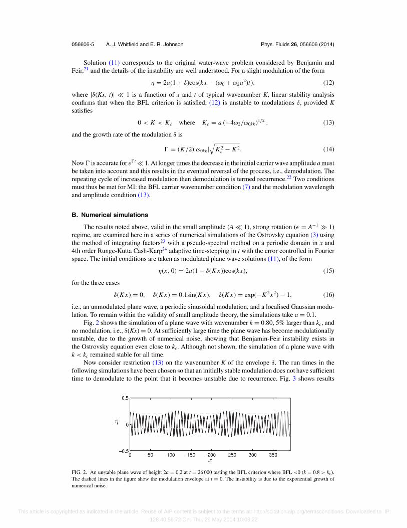
Fig. 2 shows the simulation of a plane wave with wavenumber k = 0.80, 5% larger than kc, andno modulation, i.e., δ(Kx) = 0. At sufficiently large time the plane wave has become modulationallyunstable, due to the growth of numerical noise, showing that Benjamin-Feir instability exists inthe Ostrovsky equation even close to kc. Although not shown, the simulation of a plane wave withk < kc remained stable for all time.

Now consider restriction (13) on the wavenumber K of the envelope δ. The run times in thefollowing simulations have been chosen so that an initially stable modulation does not have sufficienttime to demodulate to the point that it becomes unstable due to recurrence. Fig. 3 shows results

FIG. 2. An unstable plane wave of height 2a = 0.2 at t = 26 000 testing the BFL criterion where BFL <0 (k = 0.8 > kc).The dashed lines in the figure show the modulation envelope at t = 0. The instability is due to the exponential growth ofnumerical noise.

This article is copyrighted as indicated in the article. Reuse of AIP content is subject to the terms at: http://scitation.aip.org/termsconditions. Downloaded to IP:

128.40.56.72 On: Thu, 29 May 2014 10:08:22

056606-6 A. J. Whitfield and E. R. Johnson Phys. Fluids 26, 056606 (2014)

FIG. 3. Plane waves of height 2a = 0.2 satisfying the BFL criterion for instability (k = 0.8) with sinusoidal modulations ofdifferent wavelengths K shown relative to a frame moving at the group velocity of the carrier wave. (a) Stable modulation att = 2000 with K > Kc (K = 0.08). (b) Unstable modulation at t = 2000 with K < Kc (K = 0.06). The dashed lines in bothfigures show the modulation envelope at t = 0.

of a plane wave simulation with carrier wavenumber k = 0.80 and periodic sinusoidal modulationδ(Kx) = 0.1sin (Kx). For the case of the stable modulation K > Kc (Fig. 3(a)), a slight demodulationcan be seen from the initial condition. This is best demonstrated by noting that the height of thepeaks in the final form of the modulation is less than the original. For the modulation with K < Kc

(Fig. 3(b)) it is clear the disturbance grows as expected. Additional simulations of the periodicsinusoidal modulation, not shown in Fig. 3 were all in exact agreement with criterion (13), showingthat (13) needs to be satisfied in addition to (7) for instability to occur and that these criteria areaccurate for k within 5% of kc.

Finally, as a basis for the discussion in Sec. IV, a localised Gaussian modulation, δ(Kx)= exp (−K2x2) − 1, is considered. Here the condition δ � 1 does not hold and there is no en-velope wavenumber in the traditional sense with K serving only as a characteristic inverse lengthscale. The stability theory for modulation states that there is a critical envelope wavenumber Kc

such that all K below Kc are unstable and all K above Kc are stable. Thus it is to be expected thatfor sufficiently large K the localised structure will obey the linear theory of dispersive waves andthe structure will disperse away, and for sufficiently small K the modulation will increase due toinstability. To test this hypotheses Kc is approximated as 0.0225, where 2a has been taken in (13)to be the half height of the localised structure, and K’s are chosen such that they are sufficientlyfar away from the approximate critical envelope wavenumber Kc. Fig. 4 shows that the Gaussianmodulation for large K (Fig. 4(a)) disperses, whereas the modulation with small K (Fig. 4(b)) grows.

IV. WAVEPACKET EMERGENCE

A. Linear (strong rotation) evolution

Section III illustrated the Benjamin-Feir instability of the small-amplitude (A � 1), strong-rotation (ε = A−1 � 1), near-linear regime of the Ostrovsky equation. It is now hypothesisedthat in this regime, this instability could be the mechanism of creation for the rotationally-inducednonlinear wavepackets that have been observed to evolve from the decay of an internal solitarywave due to rotation. The proposed mechanism is that strong rotation causes an initial disturbanceto rapidly disperse into a long linear wavetrain where the amplitude and phase (and so wavenumber)of the linear wavetrain is a slowly varying function of position. This linear wavetrain is initiallystable to Benjamin-Feir instability but evolves to become unstable, selecting a particular position for

This article is copyrighted as indicated in the article. Reuse of AIP content is subject to the terms at: http://scitation.aip.org/termsconditions. Downloaded to IP:

128.40.56.72 On: Thu, 29 May 2014 10:08:22

056606-7 A. J. Whitfield and E. R. Johnson Phys. Fluids 26, 056606 (2014)

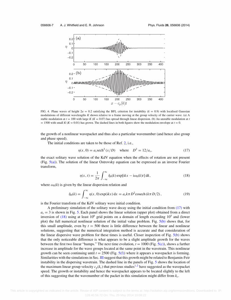
FIG. 4. Plane waves of height 2a = 0.2 satisfying the BFL criterion for instability (k = 0.9) with localised Gaussianmodulations of different wavelengths K shown relative to a frame moving at the group velocity of the carrier wave. (a) Astable modulation at t = 100 with large K (K = 0.07) has spread through linear dispersion. (b) An unstable modulation at t= 1500 with small K (K = 0.01) has grown. The dashed lines in both figures show the modulation envelope at t = 0.

the growth of a nonlinear wavepacket and thus also a particular wavenumber (and hence also groupand phase speed).

The initial conditions are taken to be those of Ref. 2, i.e.,

η(x, 0) = assech2 (x/D) where D2 = 12/as, (17)

the exact solitary wave solution of the KdV equation when the effects of rotation are not present(Fig. 5(a)). The solution of the linear Ostrovsky equation can be expressed as an inverse Fouriertransform,

η(x, t) = 1

2π

∫ ∞

−∞η0(k) exp[ikx − iω0(k)t] dk, (18)

where ω0(k) is given by the linear dispersion relation and

η0(k) =∫ ∞

−∞η(x, 0) exp(ikx) dx = askπ D2cosech (kπ D/2) , (19)

is the Fourier transform of the KdV solitary wave initial condition.A preliminary simulation of the solitary wave decay using the initial condition from (17) with

as = 3 is shown in Fig. 5. Each panel shows the linear solution (upper plot) obtained from a directinversion of (18) using at least 106 grid points on a domain of length exceeding 105 and (lowerplot) the full numerical nonlinear solution of the initial value problem. Fig. 5(b) shows that, forthis small amplitude, even by t = 500 there is little difference between the linear and nonlinearsolutions, suggesting that the numerical integration method is accurate and that consideration ofthe linear dispersive wave problem for these times is useful. Closer inspection of Fig. 5(b) showsthat the only noticeable difference is what appears to be a slight amplitude growth for the wavesbetween the first two linear “humps.” The next time evolution, t = 1000 (Fig. 5(c)), shows a furtherincrease in amplitude for the wave groups located at the same point in the wavetrain. This nonlineargrowth can be seen continuing until t = 2500 (Fig. 5(f)) where it appears a wavepacket is forming.Similarities with the simulations in Sec. III suggest that this growth might be related to Benjamin-Feirinstability in the dispersing wavetrain. The dashed line in the panels of Fig. 5 shows the location ofthe maximum linear group velocity cg(kc) that previous studies1, 2 have suggested as the wavepacketspeed. The growth or instability and hence the wavepacket appears to be located slightly to the leftof this suggesting that the wavenumber of the packet in this simulation might differ from kc.

This article is copyrighted as indicated in the article. Reuse of AIP content is subject to the terms at: http://scitation.aip.org/termsconditions. Downloaded to IP:

128.40.56.72 On: Thu, 29 May 2014 10:08:22

056606-8 A. J. Whitfield and E. R. Johnson Phys. Fluids 26, 056606 (2014)

FIG. 5. The time evolution of the linear (upper) and full nonlinear (lower) Ostrovsky equation shown relative to a framemoving at the maximum linear group velocity, cg(kc) for a KdV soliton of amplitude as = 3. (a) The initial condition,(b) t = 500, (c) t = 1000, (d) t = 1500, (e) t = 2000, and (f) t = 2500. The dashed line in (b)–(f) corresponds to a pointinitially at the origin and moving at cg(kc) and so is fixed in this frame. Note the nonlinear growth located to the left of cg(kc).

By t = 500 (Fig. 5(b)), the linear solution has dispersed sufficiently to be accurately describedusing the method of stationary phase (MSP).25 For wavenumbers away from kc, this gives the leadingorder behaviour of (18) as the sum of two slowly varying linear wavetrains,

η(x, t) ≈ η+ + η−, t → ∞, (20)

where

η+ = 2A+cos(k+x − ω0(k+)t + π/4), (21a)

η− = 2A−cos(k−x − ω0(k−)t − π/4), (21b)

with

A+ = η0(k+)[2π |c′g(k+)|t]−1/2, A− = η0(k−)[2π |c′

g(k−)|t]−1/2, (22)

This article is copyrighted as indicated in the article. Reuse of AIP content is subject to the terms at: http://scitation.aip.org/termsconditions. Downloaded to IP:

128.40.56.72 On: Thu, 29 May 2014 10:08:22

056606-9 A. J. Whitfield and E. R. Johnson Phys. Fluids 26, 056606 (2014)

FIG. 6. A comparison at t = 500 of the two-phase stationary phase approximation (dashed-dotted lines) with the full linearsolution (solid line) of the Ostrovsky equation for an initial solitary wave of amplitude as = 3 relative to a frame movingat the linear group velocity cg(kc). The envelope of the linear solution (dashed lines) was obtained by the usual Hilberttransform method. The vertical dotted lines show the measured k value for the wavepacket that eventually forms (left line)and kc (right line).

and

k±(x, t) = 6−1/2{−(x/t) ± [

(x/t)2 − 12]1/2

}1/2. (23)

The two-phase approximation (20) explains the amplitude-modulated structure that appears,strongly in the linear solution and slightly less markedly in the nonlinear solution, behind theleading packet at times t > 500. Close behind the leading packet of the wavetrain, η+ andη− have approximately the same amplitude, and wavenumbers k+ and k− lying approximatelyequidistantly above and below kc. The combined wave (20) is thus a beat pattern with orderunity modulation and carrier frequency kc. Closer to the wavefront, for x → cg(kc)t, the sta-tionary points k± coalesce at kc, giving a single packet which decays more slowly with time(t−1/3 versus t−1/2), an Airy function envelope with carrier frequency kc. This is noticeable inFig. 5(b) where the linear wavetrain is largest near the origin. The small difference between the lin-ear and nonlinear wavetrains at t = 500 means that estimates of wavepacket speed at times t < 500would return the linear value of cg(kc) (as would measurement for t < 100 for as = 4 in Fig. 8), perhapsrelated to the wavepacket speeds for small as reported in Ref. 2. Fig. 6 shows that the position wherethe wavepacket appears to begin growing (between the first two linear humps) coincides with thewavenumber of the nonlinear wavepackets that eventually emerge in the long-time full numerical sim-ulations (reported below) and that both lie to the left of the region of coalescence so that the two-phaseapproximation gives an adequate description of the wavetrain at the time and position of emergence.

Equation (20) gives an expression for a slowly varying wavetrain. Three significant differencesbetween the slightly-modulated plane wave results noted in Sec. III and (20) are that the wavetrainconsists of the superposition of two linear waves (21a), that the components η± have non-constantlocal wavenumbers k±(x, t) and that, similar to the localised Gaussian modulation example, there isno explicit envelope wavenumber as the modulation is non-periodic. To apply the results of Sec. III,we suppose that the two linear wavetrains can be treated separately, that η± vary sufficiently slowlythat the local wavenumbers k± and modulation amplitude A+ can be taken as constant, and that thewavenumber of the envelope η+ can be estimated as

K ∼ 1

A+

dA+dx

. (24)

Then, since k−(x, t) < kc, the wavetrain η− is stable to MI according to the BFL criterion (7) but,since k+(x, t) > kc, the wavetrain η+ is a candidate for MI and will be unstable if it locally also

This article is copyrighted as indicated in the article. Reuse of AIP content is subject to the terms at: http://scitation.aip.org/termsconditions. Downloaded to IP:

128.40.56.72 On: Thu, 29 May 2014 10:08:22

056606-10 A. J. Whitfield and E. R. Johnson Phys. Fluids 26, 056606 (2014)

FIG. 7. The instability index B(x, t) from (25) at various times for two different initial amplitudes as. (a) as = 3. (b) as =10. Note the larger times required in (a) for B to fall to any particular value when compared to (b), implying that instabilityoccurs at larger t for smaller initial amplitude solitary waves.

satisfies the modulation criterion (13) which becomes

B(x, t) < 4 where B(x, t) = − 1

A4+

(dA+dx

)2ωkk

ω2. (25)

If criterion (25) is satisfied at a point (x, t), then η+ should be unstable at this point, although theapproximations required to derive (25) mean that the estimate is not sharp.

Figs. 7(a) and 7(b) show plots at various times of B(x, t) for initial solitary waves of amplitude as

= 3, 10. The plots show that B has a single minimum in x/t and this minimum decreases monotonicallyin time, a property found for all as. As B decreases with time the minimum will be the first pointto cross the threshold for MI (B ∼ 4). Until then the wavetrain is locally stable and afterwards it islocally unstable. It is suggested that this is where weak nonlinear effects cause a wavepacket to growin the linear wavetrain. The crossing point fixes the time t and position x where the wavepacket startsto grow and, through (23), the carrier wavenumber, kB, of the wavepacket. The predicted carrierwavenumber kB is compared to the numerically determined value below. As with the position wherethe wavepacket appears to begin growing and the wavenumber of the nonlinear wavepackets thateventually emerge, the point where the wavetrain η+ first satisfies (25) lies within the region ofvalidity of the two-phase stationary phase approximation. To decrease to the threshold B ∼ 4, theevolution for as = 3 requires almost 40 times longer than that for as = 10. For all examples, smalleras take longer to reach the threshold and therefore it is to be expected that for smaller as instabilityoccurs at larger t, and so smaller solitary waves should take longer to form a wavepacket, a resultalso obtained in Ref. 2.

B. Numerical simulations

The predictions of Sec. IV A are examined here by numerically integrating the Ostrovskyequation to follow the decay of an internal solitary wave (17) using the same numerical methodoutlined in Sec. III with, however, a sponge region added at each end of the periodic domain toabsorb any radiation and so model computation on the physically relevant infinite domain. Previousnumerical studies2 have discussed extensively the evolution of the internal solitary wave to a nonlinearwavepacket and so here only a single example for a solitary wave with as = 4 (Fig. 8) is shown. Inagreement with Ref. 2, Fig. 8(b) shows the eventual formation of a nonlinear wavepacket from theemitted radiation. Similar to Fig. 5, the packet appears to be a consequence of nonlinear growth tothe left of the wave group at kc (the dashed line in Fig. 8). The final time in the comparable evolutionin Ref. 2 corresponds to t = 100 when the linear solution of Fig. 8(a) appears to differ little fromthe nonlinear solution of Fig. 8(b). Packet solutions arising from integrations initialised with KdVsolitons of amplitudes as = 3, 10, and 80 are shown in Figs. 9(a)–9(c). These were obtained byintegrating for a time sufficiently long that all linear radiation had separated totally from the packet.

This article is copyrighted as indicated in the article. Reuse of AIP content is subject to the terms at: http://scitation.aip.org/termsconditions. Downloaded to IP:

128.40.56.72 On: Thu, 29 May 2014 10:08:22

056606-11 A. J. Whitfield and E. R. Johnson Phys. Fluids 26, 056606 (2014)

FIG. 8. Packet emergence for an initial amplitude of as = 4 in a frame moving with the linear group velocity cg(kc). (a) Thelinear solution at t = 100. (b) The full Ostrovsky equation showing the evolution into a nonlinear wavepacket between timest = 100–1000. Note the similarity of the linear (a) and nonlinear (b) solutions at t = 100.

The integration was then continued and the packet group velocity s and period T of the packetobtained by considering the minimum of the function,

F(s, T ) =∫ L

0(η(x, 0) − η(x − sT ))2 dx

/ ∫ L

0η2(x, 0) dx, (26)

for L the length of the computational domain. The first minimum of F in the positive quadrant of(s, T) space estimates s and T and the minimum of F measures how close the solution is to periodicin the translating frame, being less than 10−5 for all converged packets discussed here. Once s andT are known other properties of a packet follow straightforwardly by considering the packet in theco-moving x − st frame. Additional solutions (e.g., that of Fig. 9(d)), referred to here as extendedpackets, were generated using a scaled packet solution of lower amplitude as an initial profile forthe evolution. Although packet solutions of the Ostrovsky equation, it appears that these extendedpackets are not accessible from initial conditions consisting of a simple isolated hump.

This article is copyrighted as indicated in the article. Reuse of AIP content is subject to the terms at: http://scitation.aip.org/termsconditions. Downloaded to IP:

128.40.56.72 On: Thu, 29 May 2014 10:08:22

056606-12 A. J. Whitfield and E. R. Johnson Phys. Fluids 26, 056606 (2014)

FIG. 9. Wave packet solutions of the Ostrovsky equation (solid lines) and their envelopes (dashed lines) created by solitarywave decay (a) as = 3, (b) as = 10, (c) as = 80, and (d) a higher, extended packet initialised using a scaled packet of loweramplitude.

The packet maximum and minimum values for solitary wave decay are shown in Fig. 10 as afunction of initial amplitude as. There is a clear asymmetry in packet maximum and minimum forlarge as (weak rotation), and a peak in packet maximum appears at as = 80, after which increasingas has negligible effect on the final packet height, as all initial KdV solitons with as � 100 evolveto the same packet. The packet asymmetry was observed in Ref. 2 as was the large as behaviour of

FIG. 10. The magnitudes of the packet maximum ηmax = max{η(x, t)} (circles) and minimum ηmin = |min{η(x, t)}|(squares) as a function of initial solitary wave amplitude as. For as � 100, all initial solitary waves appear to evolve tothe same packet solution.

This article is copyrighted as indicated in the article. Reuse of AIP content is subject to the terms at: http://scitation.aip.org/termsconditions. Downloaded to IP:

128.40.56.72 On: Thu, 29 May 2014 10:08:22

056606-13 A. J. Whitfield and E. R. Johnson Phys. Fluids 26, 056606 (2014)

FIG. 11. (a) The packet local wavenumber k as a function of x. Only the x region between the largest peak denoted k1 (whensymmetrical) and third largest peak k3 is shown. The decrease in x dependence of k with decreasing initial solitary waveamplitude supports the use of NLS theory in this regime. (b) The as = 40 packet (solid line) and its measured k (dashed-dottedline) plotted on the same x-axis to demonstrate the naming procedure for the local wavenumbers.

the maximum amplitude, discussed in more detail below. To obtain the local carrier wavenumberat any point in a packet, the instantaneous local wavelength λ(x, t) was estimated as the currentinter-peak distance at that point in the wavepacket at that time and then the time-mean of λ takenover the wave period. Fig. 11(a) gives examples of the calculated wavenumbers k(x) = 2π /λ for thepackets initialized from solitary waves with as = 3, 10, and 40. The region from the highest peak(when symmetrical), with local wavenumber denoted by k1, to the third highest peak (with localwavenumber k3) is shown, and the naming procedure for the local wavenumber is demonstrated inFig. 11(b). Only the region from the highest peak to the third highest peak is shown, since, as can beseen in Fig. 11(a), the local wavenumber appears to approach a constant beyond the third peak. Thisheld for all solutions, except the extended solutions where the determination of local wavenumbernear the third peak became inaccurate. Therefore, k1 gives a measure of the minimum k in the packetand k3 gives an approximate measure of the maximum. The relation k = 2π /λ is useful only for thenear-linear packets of Sec. IV B 1 when the carrier waves are close to sinusoidal. When there arefew crests inside the packet, as for the near-KdV packets of Sec. IV B 2 it is more useful to use thewavelength λ directly.

1. Strong rotation, small amplitude (A � 1), near-linear packets

Grimshaw and Helfrich2 note the similarity in appearance of the small amplitude wavepackets(Fig. 9(a)) to the nonlinear Schrodinger bright soliton solution. Taking the wavenumber of the carrierwave to be kc, Grimshaw and Helfrich2 thus derive an extended, higher-order NLS for the Ostrovskyequation and present envelope soliton solutions of the equation. The carrier wave has “chirped”wavenumber equal to 3kc/2 due to nonlinearity, and the solution also predicts nonlinear correctionsto both the linear phase and group velocities. The observation that the packet envelope is similarto the NLS soliton is also connected with the results here as it has been shown that from initialconditions such as localised hump perturbations to a uniform water wave9 and non-uniform initialstates in Bose-Einstein condensates,10 stable solitons can form through MI. It is thus suggested thatthe nonlinear packet in the strong rotation, small amplitude regime could be a stable soliton formedfrom MI due to weak nonlinear effects in the slowly-varying near-linear wavetrain formed by therapid dispersive destruction of the initial hump perturbation. Moreover, the observed wavenumbersin the computed packet solutions appear to lie sufficiently far from kc to suggest the standard NLS

This article is copyrighted as indicated in the article. Reuse of AIP content is subject to the terms at: http://scitation.aip.org/termsconditions. Downloaded to IP:

128.40.56.72 On: Thu, 29 May 2014 10:08:22

056606-14 A. J. Whitfield and E. R. Johnson Phys. Fluids 26, 056606 (2014)

FIG. 12. (a) The envelope of the as = 4 converged packet (solid line), along with the envelope predictions from the standardNLS (dashed line) and higher-order NLS (dashed-dotted line), both with the A2 correction. The standard NLS with A2

correction is indistinguishable from the as = 4 converged packet. (b) and (c) Details of the extrema of the packet in (a)with the symmetrical standard NLS envelope prediction without the A2 correction (dotted line) included. The A2 correctionaccurately captures the asymmetry of the packet.

bright soliton as an accurate model. This section tests the accuracy of the standard NLS soliton inthe strong rotation regime.

For k > kc (unstable) the standard NLS has bright soliton solution,

A = a sech(K X ) exp(−iσ t) where K = a (−ω2/ω0kk)1/2 , σ = ω2a2/2, (27)

which corresponds in the original problem to the asymptotically correct solution,

η ≈ 2a sech[K (x − cgt)] cos[k(x − cct)] a � 1, (28)

where cc = (ω0 + σ )/k is the phase speed of the carrier wave. One shortcoming of solution (28) is itsup-down symmetry as Fig. 10 suggests that an accurate model should display up-down asymmetryas found in the packets. The next term A2 in expansion (8) has precisely the correct asymmetry andcan be written2 in the form A2 = χA2 where χ = 2k2/(12k4 + 3). Including this term gives in theoriginal problem, correct to second-order in the amplitude, the solution

η ≈ 2a sech[K (x − cgt)] cos[k(x − cct)] + 2a2χsech2[K (x − cgt)] cos[2k(x − cct)]. (29)

Fig. 12 gives a detailed comparison of solutions (28) and (29) with the numerically determinedpacket for as = 4. The value of the carrier wavenumber is taken as k = k1, which is effectively constantthroughout the packet as shown by Fig. 11(a), and amplitude a = (max{η(x, t)} − min{η(x, t)})/2.Fig. 12(a) shows that (29) is graphically indistinguishable from the numerically determined packet.Fig. 12(a) also includes the higher-order NLS soliton from Ref. 2 (including its second-ordercorrection) which appears to be a less accurate model of the packet for these parameters. Figs. 12(b)and 12(c) give details near the extrema of the packet, including the solution (28) and thus showingthat the term A2 not only captures the asymmetry but also significantly increases the accuracy of thesolution.

To further test the asymptotic validity of the (28) and (29) solutions, the Ostrovsky equationwas integrated numerically taking (28) and (29), with the parameters of Fig. 12, as initial conditions.Fig. 13 shows the mean squared deviation (MSD) from the initial condition,

∫[η(x, t) − η(x, 0)]2 dx

measured when a crest is at the origin (x-symmetric), as a function of time. Although the standardNLS packet with A2 correction appears indistinguishable from the numerical packet solution inFig. 12, Fig. 13 shows the MSD converging to a deviation slightly less than 0.007. This constantdeviation appears to arise from the absence in the NLS solution (29) of exponentially small “tails”(discussed in depth below) found in the converged packets. Fig. 13 also includes the MSD for the

This article is copyrighted as indicated in the article. Reuse of AIP content is subject to the terms at: http://scitation.aip.org/termsconditions. Downloaded to IP:

128.40.56.72 On: Thu, 29 May 2014 10:08:22

056606-15 A. J. Whitfield and E. R. Johnson Phys. Fluids 26, 056606 (2014)

FIG. 13. The mean-squared-deviation (MSD) from the initial state for numerical integrations of the Ostrovsky equation withthe standard and higher-order NLS solitons (with and without the A2 correction) set as the initial conditions as a function oftime, t. The parameters used are those for the NLS solitons for the as = 4 packet in Fig. 12.

higher-order NLS soliton of Fig. 12 which increases monotonically indicating perhaps that thishigher-order NLS soliton with k = kc is not as close to an asymptotic solution of the Ostrovskyequation for these parameter values.

Fig. 14 shows the wavenumber estimate kB from Sec. IV A with the k1 and k3 wavenumbersas a function of initial solitary wave amplitude as. The values of k1 and k3 from the numericalsolutions are all greater than kc ≈ 0.76, thus satisfying the wavenumber criterion (7) for instability,and the agreement with kB is reasonable. NLS theory predicts a constant k for a given as as shownby the coincidence of k1 and k3 up to as ∼ 10, i.e., ηmax ∼ 3 (see also Fig. 11(a)). For larger as

(approaching the weak-rotation, near-KdV region) the wavenumber varies with x as these largerwaves are too strongly nonlinear for the weakly-nonlinear NLS approximation to apply. The endsof the packet should merge with the linear theory and so it is to be expected that kB would predict k3

(closer to edge of the packet) more closely than k1, and this is indeed seen in the solutions. Over theentire range of as here, kB estimates k3 to within 16%, lying always between k3 and the higher-orderNLS prediction2 of 3kc/2. The small deviation of kB from k3 might be ascribable to the growth ofnearby k once a band of wavenumbers is unstable, to inaccuracies in the two-phase stationary phaseapproximation for k near kc, or to the approximations required to derive the criterion (25).

Figs. 15 and 16 show the phase velocity c1 measured at the middle of the packet (the pointassociated with the wavenumber k1) and the group velocity s of the numerical solutions, along withthe velocity predictions cc(k1), cg(k1) (using the numerically determined k1) from the soliton solution

FIG. 14. The wavenumber predictions from modulation instability (kB, dashed line), higher-order NLS (3kc/2, dashed-dottedline), and numerical measurements k1 (squares) and k3 (circles).

This article is copyrighted as indicated in the article. Reuse of AIP content is subject to the terms at: http://scitation.aip.org/termsconditions. Downloaded to IP:

128.40.56.72 On: Thu, 29 May 2014 10:08:22

056606-16 A. J. Whitfield and E. R. Johnson Phys. Fluids 26, 056606 (2014)

FIG. 15. Maximum phase velocity (middle of the packet) predictions, cc(k1) (circles), and higher-order NLS (dashed-dottedline), along with the numerical measurements c1 (squares). The agreement between c1 and cc(k1) is close for ηmax � 5.

(28) and (29) and the extended NLS. The predictions from the standard NLS soliton solution areindistinguishable from the numerically determined values in the small amplitude regime, ηmax � 5.

While the agreement of the numerics with the standard NLS theory is good, it should benoted that the observed wavenumbers of the smallest amplitude packets are close to kc where thesecond-order dispersion term (ω0kk) in the NLS is zero. As noted in Ref. 2, for sufficiently smallω0kk, the effect of third-order dispersion ω0kkk = d3ω0/dk3 must be considered. The NLS for wavegroups near the zero-dispersion point (k = kc) can be written2

iAt + 12ω0kk AX X − ω2|A|2 A = i 1

6ω0kkk AX X X , (30)

where the term on the right-hand side gives the effect of third-order dispersion. To investigate thenecessity of including the higher-order dispersion, the two dispersive terms are plotted alongsideeach other in Fig. 17 for two of the smallest converged packets (as = 3, 6). Fig. 17 shows that thesecond-order dispersion term dominates helping to explain why the properties of these packets areso well described by the standard NLS. However, third-order dispersion can be as much as 10% ofsecond-order dispersion in places and so it is likely that it will have some effect. Because of therelative smallness of third-order dispersion it can be considered as a small perturbation in (30). For aNLS bright soliton this perturbation introduces exponentially small trailing oscillations12 or “tails”and these are seen upon close examination of the small amplitude converged packets. It was toobtain an explicit soliton solution without radiative leakage that Grimshaw and Helfrich2 followedthe approach from nonlinear optics of including higher-order mixed nonlinear-dispersive terms in

FIG. 16. Group velocity predictions, cg(k1) (circles) and higher-order NLS (dashed-dotted line), along with numericalmeasurements s (squares). The agreement between s and cg(k1) is close for ηmax � 7.

This article is copyrighted as indicated in the article. Reuse of AIP content is subject to the terms at: http://scitation.aip.org/termsconditions. Downloaded to IP:

128.40.56.72 On: Thu, 29 May 2014 10:08:22

056606-17 A. J. Whitfield and E. R. Johnson Phys. Fluids 26, 056606 (2014)

FIG. 17. The magnitudes of the second-order (|ω0kkAXX/2|, solid line) and third-order (|ω0kkkAXXX/6|, dashed line) lineardispersive terms of the NLS equation for the (a) as = 3 and (b) as = 6 converged packets. The oscillations on the left of thefigures are caused by exponentially small tails.

their governing equation. However they note, as has been seen above, that these higher-order termsdo not appear to improve agreement with the numerical solutions. Fig. 18 shows the packet half-amplitude, |A|, for the converged packets as = 3 and as = 4 plotted on a highly vertically expandedscale. The tails are clearly visible and are closely comparable to those in Fig. 2 of Ref. 12.

Wai, Chen, and Lee12 derived predictions for the wavenumber and amplitude of the tails whichwere later refined by Grimshaw.13 In order to compare the results here with those of Ref. 13, (30) iswritten in its canonical form using the scalings T = t/|ω0kk|, A = |ω0kk/ω2|1/2φ and the transformationsφ = ψ*, X = −Y to give the equation

iψT + 12ψY Y + |ψ |2ψ = iβψY Y Y with β = |ω0kkk/ω0kk |/6. (31)

The wavenumber prediction k ∼ 1/(2β) from Ref. 13 gives, for the as = 3 and as = 4 packets, tailwavenumbers of 0.31 and 0.47, respectively, to be compared with the numerically determined valuesof 0.17 and 0.89. The corresponding tail amplitude predictions (in the transformed coordinates) are10−13 and 10−5 to be compared with the measured values of 10−4 and 10−4. Apart from the as = 3tail amplitude, the predictions appear reasonable given the difficulty of measuring such small terms

FIG. 18. The packet half-amplitude |A| plotted on a highly vertically expanded scale for the (a) as = 3 and (b) as = 4converged packets showing the oscillating tails caused by third-order dispersion.

This article is copyrighted as indicated in the article. Reuse of AIP content is subject to the terms at: http://scitation.aip.org/termsconditions. Downloaded to IP:

128.40.56.72 On: Thu, 29 May 2014 10:08:22

056606-18 A. J. Whitfield and E. R. Johnson Phys. Fluids 26, 056606 (2014)

FIG. 19. Weak-rotation (large amplitude) packet wavelength measurements λ1 (circles) and λ3 (squares) for packets arisingfrom KdV solitary wave decay and λ1 (stars) and λ3 (diamonds) from extended solutions. Note here λ1 and λ3 refer to thesame positions in the wavepacket as k1 and k3, respectively (see Fig. 11(b)).

in an evolving flow, since here the envelope has been obtained from the full numerical solution ofthe Ostrovsky equation and, so includes the carrier wave, whereas the integrations in Ref. 12 are forthe envelope equation (31) only.

2. Weak-rotation (ε = A−1 � 1), near-KdV wavepackets

As noted in Sec. II, when the scaling in this region is chosen as the appropriate KdV scaling forη, x, and t, the governing equation transforms to (3) with coefficient ε2 = A−2 � 1 on the right-handside, giving the small rotational perturbation to the KdV. This is precisely the equation considered byGilman, Grimshaw, and Stepanyants18 and the wavepackets in the weak-rotation regime here havemany features in common with the solutions presented there. The weakness of rotational effectsmeans that the initial KdV soliton persists for relatively long (KdV-scaled) times, decaying onlyslowly due to linear wave radiation.2, 14 By determining this linear radiation Grimshaw and Helfrich2

predict that in this regime the wavepacket amplitude should oscillate with decaying amplitude abouta fixed constant value as as → ∞, precisely as seen in Fig. 10, where all initial conditions with as �100 evolve to the same limit packet (referred to as the KdV-IC-limit packet below) with ηmax ∼ 20and so ε ∼ 0.05. Grimshaw and Helfrich2 point out that for sufficiently small initial conditions themodel of a radiating KdV soliton is inappropriate as the radiated wavetrain cannot separate from theleading soliton. This corresponds to the strong-rotation, near-linear regime, described above, wherethe wavepacket appears to arise from MI in the dispersive wavetrain behind the leading disturbance.Converged higher amplitude, weaker rotation (and so smaller ε) extended wavepackets are obtained

FIG. 20. Weak-rotation (large amplitude) maximum phase velocity (middle of the packet) measurements, c1, of packetscreated from solitary wave decay (squares) and from extended solutions (diamonds).

This article is copyrighted as indicated in the article. Reuse of AIP content is subject to the terms at: http://scitation.aip.org/termsconditions. Downloaded to IP:

128.40.56.72 On: Thu, 29 May 2014 10:08:22

056606-19 A. J. Whitfield and E. R. Johnson Phys. Fluids 26, 056606 (2014)

FIG. 21. Weak-rotation (large amplitude) group velocity measurements, s, of packets created from solitary wave decay(squares) and from extended solutions (diamonds).

from evolutions initialised with scaled converged packets from solitary wave decay. Figs. 19–21show the computed wavelength, phase and group velocities for the higher amplitude solutions andextended solutions. Note that on each graph there are 5 entries for ηmax ∼ 20 corresponding to thefive integrations for as � 100 which all evolve to the KdV-IC-limit packet.

The Ostrovsky equation has an exact parabolic solution18 and a notable feature of the higheramplitude packets is that the lower envelope of the packet becomes increasingly close to parabolicwith the packet solutions taking the appearance of a train of solitary waves propagating adiabatically18

through a more slowly-varying background state of finite extent. Their dynamics is thus similar tothat described in Ref. 18 where a single solitary wave is shown propagating adiabatically throughan infinite periodic background. To quantify this observation a parabola

η = α2(ζ − ζ0)2 + α0 where ζ = x − st, (32)

was fitted by least squares to the bottom 40% of the lower envelope of the solutions. The values ofα2 for these weak-rotation solutions are shown in Fig. 22 and the parabolas for the KdV-IC-limitpacket from as = 400 and the largest extended solution are shown in Figs. 23(a) and 23(b). Thefit in both examples is good. The value of α2 for the KdV-IC-limit packet from as = 120, 160,

FIG. 22. The quadratic coefficient α2, obtained from a least squares fit of a parabola to the lower envelope of the weak-rotation (large amplitude) wavepackets, as a function of (a) the initial solitary wave amplitude as, and (b) the maximum wavepacket height ηmax. The dashed line represents the Ostrovsky parabola value, α2 = 1/6. The KdV-IC-limit packets formedfrom the decay of a solitary wave appear to have the same value of α2 as the Ostrovsky parabola.

This article is copyrighted as indicated in the article. Reuse of AIP content is subject to the terms at: http://scitation.aip.org/termsconditions. Downloaded to IP:

128.40.56.72 On: Thu, 29 May 2014 10:08:22

056606-20 A. J. Whitfield and E. R. Johnson Phys. Fluids 26, 056606 (2014)

FIG. 23. Weak-rotation (large amplitude) packet solutions (dashed lines) for a solution created by solitary wave decay (a)the KdV-IC-limit packet from as = 400 and an extended solution (b), along with the fitted parabolas (solid lines) and thelower packet envelopes (dashed-dotted lines).

200, 300, and 400 coincides with the exact parabolic solution of the Ostrovsky equation for whichα2 = 1/6 (Fig. 22(a)), but the velocity prediction from the Ostrovsky parabola of s = −2α0 (α0

∼ −9.5) differs in both direction and magnitude, from the packet envelope velocity. This appearsto reflect an interaction between the solitons within the packet and the slowly-varying (when KdV-scaled) background. The parabolic fit for the extended packets is even closer (Fig. 23) but the valuesfor α2 exceed 1/6 (Fig. 22(b)). This might be related to their being inaccessible from single humpinitial conditions. Similar to the small amplitude, strong rotation packets, all weak-rotation packetsappeared to have tails. Fig. 24 shows the KdV-IC-limit packet (as = 400) on a vertically expandedscale. Unlike the tails in the near linear regime which show modulations in their amplitude, the tailamplitude here appears to be independent of x.

V. DISCUSSION

An accurate numerical method has been presented for determining wavepacket solutions of theOstrovsky equation by requiring that the normalized mean-square-deviation (26) over one periodin the co-moving frame is at most 10−5. Using this method converged wavepacket solutions of theparameter-free Ostrovsky equation (3) have been obtained with amplitudes covering the range fromηmax = 0.1 to ηmax = 40. The precision of the method allows accurate measurement of the phasespeed and local wavenumber for individual crests, and the shape and group speed of the packetenvelopes. The envelopes can be divided conveniently into two regimes: a small amplitude, strong

FIG. 24. A snapshot of the KdV-IC-limit packet (as = 400) packet showing a typical tail in the weak-rotation limit.

This article is copyrighted as indicated in the article. Reuse of AIP content is subject to the terms at: http://scitation.aip.org/termsconditions. Downloaded to IP:

128.40.56.72 On: Thu, 29 May 2014 10:08:22

056606-21 A. J. Whitfield and E. R. Johnson Phys. Fluids 26, 056606 (2014)

rotation, near linear regime, where the relevant small parameter is the wavepacket amplitude, and aweak-rotation, near KdV regime where the relevant small parameter, measuring the strength of therotation, is the inverse of the amplitude of the packet in the parameter-free Ostrovsky equation.

In the near linear regime the computed wavenumber, k, of the carrier wave takes a unique constantvalue throughout each packet. This value of k gives immediately a unique linear group speed throughthe linear dispersion relation (5) and this speed coincides with the numerically determined groupspeed of the packets (Fig. 16). This leads to the hypothesis that the packets can be modelled as brightsolitons of the NLS equation. With the carrier wavenumber k determined, the only free parameter inthe expression for the NLS soliton (29) is the amplitude, a = (max{η(x, t)} − min{η(x, t)})/2. Witha determined for each packet, the phase speed is given immediately through (27), a weakly-nonlinearcorrection to the linear dispersion relation, and once again this speed coincides with the numericallydetermined speed of crests within the packets (Fig. 15). The amplitude a and wavenumber k uniquelydetermine the packet shape through (29) and, in particular, its asymmetry due to second-order (ina) terms is given immediately. These packet shapes closely model the numerically determinedwavepackets (Fig. 12). The accuracy of this NLS packet is confirmed by taking the packet as theinitial condition in the Ostrovsky equation and demonstrating that the solution deviates little fromthe initial condition during the evolution (Fig. 13).

Grimshaw and Helfrich2 point out that the wavenumbers of the packets can be expected to benear k = kc, the wavenumber corresponding to the maximum of the group velocity. Precisely atk = kc the second-order dispersion of the usual NLS equation vanishes and third-order dispersiondominates and thus Grimshaw and Helfrich2 derive a higher-order NLS equation which incorporatesthe effects of both second and third-order dispersion. A model2 of the packets obtained by settingk = kc in this higher-order NLS equation seems less successful in its predictions than the standardNLS soliton (29). This is perhaps explained by Fig. 17 which shows that, throughout the numericallydetermined wavepackets, second-order dispersion is approximately 10 times larger than third-orderdispersion. Third-order dispersion can thus be treated as a small perturbation to the soliton (29),following Grimshaw,13 leading to a prediction of exponentially small tails which are indeed observed(Fig. 18) and closely resemble those in Fig. 2 of Wai, Chen, and Lee.12

Modulational instability generates solitons from initial hump perturbations in water waves9 andBose-Einstein condensates10 and thus is suggested as a possible mechanism for the wavepacketsobserved in the strong rotation, near linear regime here. Standard results are applied by noting that anyinitial disturbance rapidly disperses into a linear wavetrain with slowly varying local wavenumberand amplitude. Over much longer times weakly nonlinear effects allow MI of this wavetrain anda local instability criterion (25), which must be satisfied in addition to the carrier wavenumbercondition (7), is suggested. The MI growth rate increases as k increases above kc, whereas lineararguments here and previously2 suggest that disturbance energy disperses slowest near k = kc.Criterion (25) captures the competition between these two effects, predicting the position and timewhen a nonlinear packet should first appear and an estimate of the carrier wavenumber for the packet,all of which are in accord with the numerically determined values (Fig. 14).

In the weak-rotation limit the initial KdV soliton does not disperse rapidly but persists forrelatively long (KdV-scaled) times, decaying only slowly due to linear wave radiation.2, 14 Sufficientlylarge initial solitons (sufficiently weak rotation, as � 100) all evolve to the same KdV-IC-limitpacket of Fig. 23(a) as predicted by Grimshaw and Helfrich2 by considering the weak radiatedlinear wavefield. The wavepackets are shown to resemble a wavetrain of KdV solitons propagatingadiabatically through a slowly varying (KdV-scaled) parabolic background of finite extent, withdynamics exactly those of the single KdV soliton on the infinite periodic background of Gilman,Grimshaw, and Stepanyants.18 These wave packets also appear to possess exponentially small tails.The analytical questions raised by the observations are under investigation.

ACKNOWLEDGMENTS

The authors are grateful to two anonymous referees whose questions and comments led to aclearer exposition. A.J.W. was supported by UCL Mathematics Department under the Wren Bequestand Sir James Lighthill Scholarships.

This article is copyrighted as indicated in the article. Reuse of AIP content is subject to the terms at: http://scitation.aip.org/termsconditions. Downloaded to IP:

128.40.56.72 On: Thu, 29 May 2014 10:08:22

056606-22 A. J. Whitfield and E. R. Johnson Phys. Fluids 26, 056606 (2014)

1 K. R. Helfrich, “Decay and return of internal solitary waves with rotation,” Phys. Fluids 19, 026601 (2007).2 R. H. J. Grimshaw and K. R. Helfrich, “Long-time solutions of the Ostrovsky equation,” Stud. Appl. Math. 121, 71–88

(2008).3 M. Stastna, F. J. Poulin, K. L. Rowe, and C. Subich, “On fully nonlinear, vertically trapped wave packets in a stratified

fluid on the f-plane,” Phys. Fluids 21, 106604 (2009).4 K. R. Khusnutdinova and K. R. Moore, “Initial-value problem for coupled Boussinesq equations and a hierarchy of

Ostrovsky equations,” Wave Motion 48, 738–752 (2011).5 R. H. J. Grimshaw, K. R. Helfrich, and E. R. Johnson, “Experimental study of the effect of rotation on nonlinear internal

waves,” Phys. Fluids 25, 056602 (2013).6 D. Farmer, Q. Li, and J.-H. Park, “Internal wave observations in the South China Sea: The role of rotation and non-linearity,”

Atmos.-Ocean 47, 267–280 (2009).7 Q. Li and D. M. Farmer, “The generation and evolution of nonlinear internal waves in the deep basin of the South China

Sea,” J. Phys. Oceanogr. 41, 1345–1363 (2011).8 V. Vlasenko, J. C. Sanchez Garrido, N. Stashchuk, J. Garcia Lafuente, and M. Losada, “Three-dimensional evolution of

large-amplitude internal waves in the Strait of Gibraltar,” J. Phys. Oceanogr. 39, 2230–2246 (2009).9 V. I. Shrira and V. Geogjaev, “What makes the Peregrine soliton so special as a prototype of freak waves?” . Eng. Math.

67, 11–22 (2010).10 L. D. Carr and J. Brand, “Spontaneous soliton formation and modulational instability in Bose-Einstein condensates,” Phys.

Rev. Lett. 92, 040401 (2004).11 R. H. J. Grimshaw, D. Pelinovsky, E. Pelinovsky, and T. Talipova, “Wave group dynamics in weakly nonlinear long-wave

models,” Phys. D 159, 35–57 (2001).12 P. Wai, H. Chen, and Y. Lee, “Radiations by “solitons” at the zero group-dispersion wavelength of single-mode optical

fibers,” Phys. Rev. A 41, 426 (1990).13 R. Grimshaw, “Weakly nonlocal solitary waves in a singularly perturbed nonlinear Schrodinger equation,” Stud. Appl.

Math. 94, 257–270 (1995).14 R. H. J. Grimshaw, J.-M. He, and L. A. Ostrovsky, “Terminal damping of a solitary wave due to radiation in rotational

systems,” Stud. Appl. Math. 101, 197–210 (1998).15 M. J. Ablowitz and H. Segur, Solitons and the Inverse Scattering Transform, Studies in Applied Mathematics Series

(Society for Industrial and Applied Mathematics, 2006).16 R. H. J. Grimshaw and K. R. Helfrich, “The effect of rotation on internal solitary waves,” IMA J. Appl. Math. 77, 326–339

(2012).17 M. Stastna and K. Rowe, “On weakly nonlinear descriptions of nonlinear internal gravity waves in a rotating reference

frame,” Atl. Electron. Math. 2, 30 (2007).18 O. A. Gilman, R. H. J. Grimshaw, and Y. A. Stepanyants, “Dynamics of internal solitary waves in a rotating fluid,” Dyn.

Atmos. Oceans 23, 403–411 (1996).19 M. J. Lighthill, “Contributions to the theory of waves in non-linear dispersive systems,” IMA J. Appl. Math. 1, 269–306

(1965).20 H. Hasimoto and H. Ono, “Nonlinear modulation of gravity waves,” J. Phys. Soc. Jpn. 33, 805–811 (1972).21 T. B. Benjamin and J. E. Feir, “The disintegration of wave trains on deep water,” J. Fluid Mech. 27, 417–430 (1967).22 A. M. Kamchatnov, Nonlinear Periodic Waves and Their Modulations: An Introductory Course (World Scientific Publishing

Company, Incorporated, 2000), p. 305.23 L. N. Trefethen, Spectral Methods in MATLAB, Vol. 10 (Society for Industrial and Applied Mathematics, 2000), p. 111.24 J. R. Cash and A. H. Karp, “A variable order Runge-Kutta method for initial value problems with rapidly varying right-hand

sides,” ACM Trans. Math. Software (TOMS) 16, 201–222 (1990).25 S. A. Orszag and C. M. Bender, Advanced Mathematical Methods for Scientists and Engineers (McGraw Hill, New York,

1978), p. 276.

This article is copyrighted as indicated in the article. Reuse of AIP content is subject to the terms at: http://scitation.aip.org/termsconditions. Downloaded to IP:

128.40.56.72 On: Thu, 29 May 2014 10:08:22