. . . . _ .. . . . -

I

. .

ROTATIONAL MOTIONS OF SATELLlTES IN A RADIAL GRAVITY FIELD

by Kurt Magnus

June 1963

GPO PRICE S-

OTS PRICEtS) S-

Microfiche (MF)

. . -

UNIVERSITY OF KANSAS CENTER FOR RESEARCH IN ENGINEERING SCIENCE

Lawrence, Kansas \

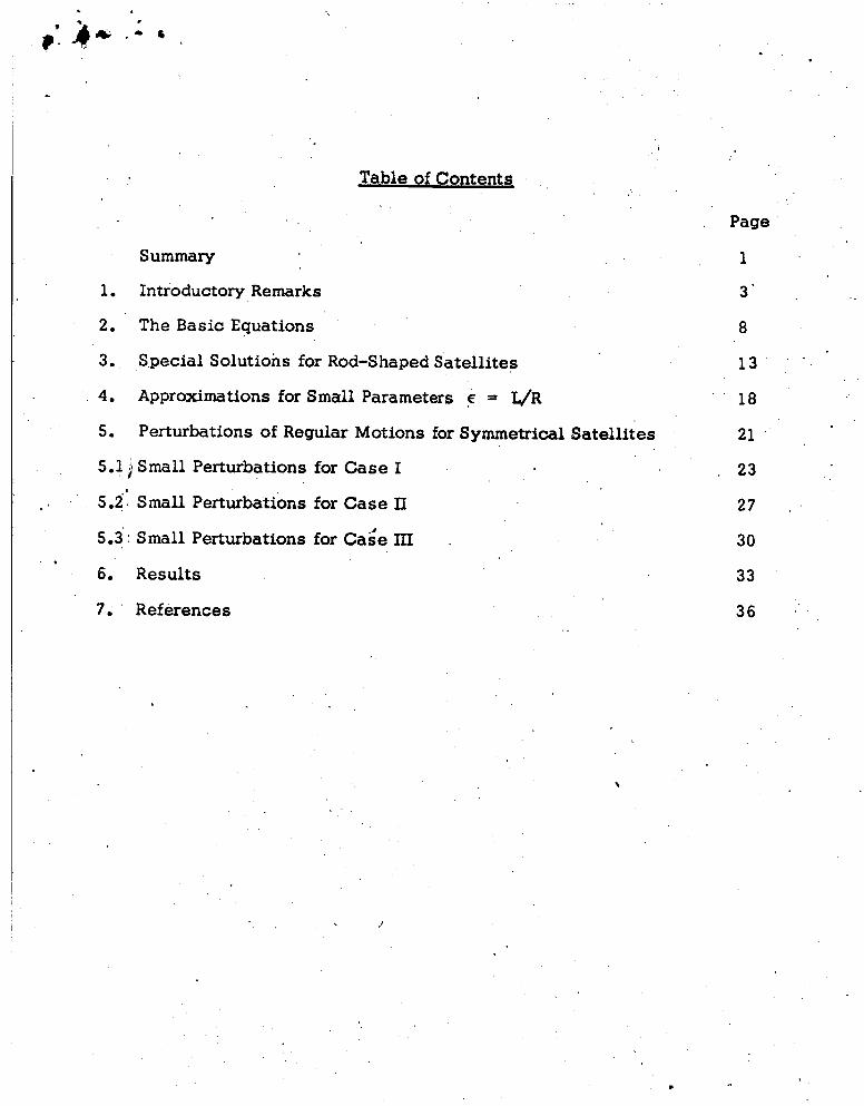
Table of Contents

Summary

1 . Introductory Remarks

2. The Basic Equations

3 . Special Solutions for Rod-Shaped Satellites

4. Approximations for Small Parameters 5 = L / R

5 Perturbations of Regular Motions for Symmetrlcal satellites

5.1 j Small Perturbations for Case I

5.2': Small Perturbations for Case II

5.3 : Small Perturbations for CaGe 111

6. Results

7. ' References

. Page

1

3'

8

13

' ' 18

21

. 23

27 .

30

33

36

1

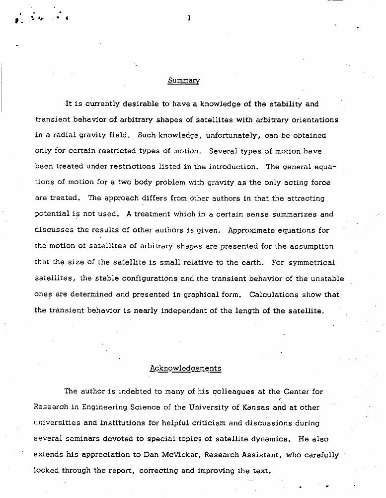
Summary

It is c k e n t l y desirable to have a knowledge of the stability and

transient behavior of arbitrary shapes of satellites with arbitrary orientations

in a radial gravity field. Such knowledge, unfortunately, can be obtained

only for certain restricted types of motion. Several types of motion have

been treated under restrictions listed in the introduction.

tions of motion for a two body problem with gravity as the only acting force

are treated.

The general equa-

The approach differs from other authors in that the attracting

potential is not used. A treatment which in a certain sense summarizes and

discusses the results of other authors is given. Approximate equations for

the motion of satellites of arbitrary shapes are presented for the assumption

that the size of the satellite is small relative to the earth. For symmetrical

satellites, the stable configurations and the transient behavior of the unstable

ones are determined and presented in graphical form. Calculations show that

the transient behavior is nearly independent of the length of the satellite.

Acknowledgements

The author is indebted to many of h i s colleagues at the Center for r

Research in Engineering Science of the University af Kansas and at other

universities and institutions for helpful criticism and discussions during

several seminars devoted to special topias of satellite dynamics. He also . extends his appreciation to Dan McVickar, Research Assistant, who carefully '

looked through the report, correcting and improving the text.

. *

.I

' . * 1 t . .

2

. The research described in this report was performed primarily during

the academjc year 1962 - 1963 while the ;rrlthcx WGS ii 'v'isiting Professor at

the University of Kansas and a Member of the Center for Research in Engineering

Science in Lawrence, Kansas. The National Aeronautics and Space Administration

sponsored the final phases of the work and publication of results through NASA

Research Grant NsG 298-62. . -

~

. -

3

1. Introdiictcn~ Ecmaiks

Motions of celestial bodies having nearly spherical ellipsoids of

inertia are usually described with sufficient accuracy by the Kepler equations . In mechanics of satellites however, motions of rod-shaped and disc-shaped

bodies are also of interest. Therefore, more general equations for a two-body

problem must be considered.

The differential equations of motion for the mutual gravitational

attraction of two finite rigid bodies contain the equations for forces and

torques. These equations describe position and angular velocity of the

satellite but are complicated by the coupling of vibrational and orbital motions.

It is necessary to combine these equations with geometrical equations of the

satellite to describe its orientation in space.

Certain aspects of this problem have been treated by several authors

in recent years . Roberson made general calculations for the gravitational

torques acting about the center of mass of a satellite (1) and also derived

general equations for rotational motions of satellites with moving parts inside

(2). The same problem was treated by Lurye'(3); however, neither author gave

a solution for a practical system of coordinates. In a series of publications,

Duboschin (4, 5, 6) treated several aspects of rotational motion. After deriving

general equations for the motion of n rigid bodies with gravitational attraction,

he restricts his consideration to a two-body problem with a homogeneous

sphere (earth) and a rod-shaped satellite. For this case, three special

.

solutions -- the so-called "regular motions" -- were calculated. Up to now,

these solutions seem to be the only exact solutions for-the equations in question.

.

4

Considerations concerning these special solutions are discussed in detail in

Chapter 3. Duboschir, (6) cko gave approximate results for satellites with

symmetrical ellipsoids of inertia. However, because he uses a system of

sophisticated variables, physical interpretation of his results is difficult.

Parts of his discussion are therefore completed and extended in Chapter 3.-

There are also other publications related to the problem in question.

Davis (7) calculated possible vibrations of a simplified satellite consisting

of two masses separated by.a fixed distance (dumbbell-shaped). However,

generalization of these results to satellites with arbitrary shapes does not

m e e t the requirements of an exact mathematical analysis. The simplifications

involved require that the results be interpreted with extreme caution. Stocker ,

and Vachino (8) treated a special case of motion of a dumbbell-shaped satel-

lite in an elliptical orbit. Their results show that vibrations of the dumbbell

axis in the orbital plane can take place with varying amplitude and frequency.

Angular motions of bodies of arbitrary shape were calculated by Suddath (9).

But, because he neglects the coupling between orbital and rotational motion

and assumes special kinds of acting torques not corresponding to gravitational

torques, his considerations do not apply to the type of motion of interest in

this investigation. The same applies to an investigation cohducted by Cole,

Epstrand, and O'Neill (10).

torques and solve the classical equations for the rotation of a rigid body for

several cases of special external torques.

.

They neglect from the start the gravitational

At the t i m e that this investigation was nearing completion, the author

became aware of several other reports related to this subject. They are listed

as numbers 11 to 14 in the references. The essence of each report is briefly

5

stated. Klemperer (11) indicated an exact solution for the vibrations in the

plana rllf the orhit sf a &iiiibbell-shapea satellite. His solution is analogous

to the familiar motion of a pendulum and can be expressed byselliptical inte-

grals. Beletskiy (12) calculated the stability of the positions of equilibrium

relative to the earth for non-spinning satell i tes of arbitrary shape. His cal-

culations are valid for the more general elliptical orbit, but they are restricted

to satellites which are s m a l l relative to the earth. Thomson (13) treated the

special case of a symmetrical satellite in a circular orbit oriented such that

i t s axis of symmetry is perpendicular to the plane of the orbit. His calculations

of the amount of spin necessary to stabilize the satellite appear in figure 5 of

this report in a completed form. Thomson only calculated the region of vibra-

tional instability, whereas fig. 5 contains the region of asymptotic instability

as well. A very comprehensive study of the investigations .,which have been

conducted in the field of stability of satellites is presented in a Ph.D. thesis

by DeBra (14) -. His personal contribution concerns the effects which ellipticity

of the orbit, oblateness of the earth, and inner damping have on stability of

the satellite.

The following considerations sha l l contribute to an understanding of

the complicated motions of satell i tes in orbit. Because the practical problem

is an extremely difficult one, this investigation is restricted by the following

assumptions:

1 e Forces and torques arising from atmospheric resistance, magnetic fields, and solar-pressure shall be neglected.

2 . Classical Newtonian mechanics and the Newtonian gravi- tational law shall be valid.

3. Only a two body problem I s treated; effects of other celestial bodies are neglected.

. b

6

4. The earth is a homogeneous sphere (or is composed of homogeneous concentric spherical shells).

5. The center of mass of t h e whole system (earth and satellite) is stationary or moves without acceleration.

6. The satellite is a rigid body.

In Chapter 4, it will furthermore be assumed that the dimensions of

the satellite are small compared with t h e radius of the earth. Special assump-

tions concerning the shape of the satellite are made in Chapter 3 where a rod-

shaped satellite is treated and in Chapter 5 where ellipsoids of inertia are

assumed to be rotational ellipsoids.

This restricted problem is much simpler than the real motion of satel-

lites. But, considering our present state of knowledge, the problem can only

be formulated clearly with these restrictions.

Extreme caution must be observed in calculating the behavior of

satellites due to the difference between celestial and terrestrial mechanics.

Effects negligible in terrestrial mechanics a re frequently quite appreciable in

celestial mechanics. An example is the concept of center of gravity which 1 .

cannot be used in this treatment. A center of gravity simply does not exist

because the directions of the resulting gravity forces do not pass through a

fixed "center" in the body i f the orientation of the body in the radial gravity

field varies. This investigation reveals that , even for very s m a l l satellites,

these effects cannot be neglected i f long periodic motions are of interest,.

The basic equations are given not in potential form but in vector

notation, using the equations of equilibrium of forces and torques. Also,

the geometrical description of body orientation shall be presented in a some-

what different way from mos t of the other authors. The well-known Euler-angles

t j

case 0 = 0 , It is t.".S&ie iiiciie convenient to take either the directional

cosines oianother set of angles. This makes it easier to interpret the physi-

cal significance of theoretical results.

vtiTr, 8 shall not be used because they lose their uniqueness in the special

t %

. .

. '

. .

. .

8

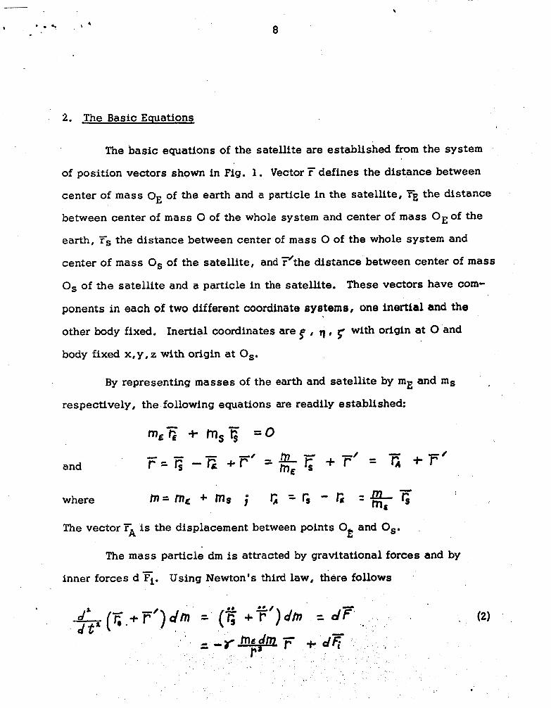
' 2. The Basic Equations

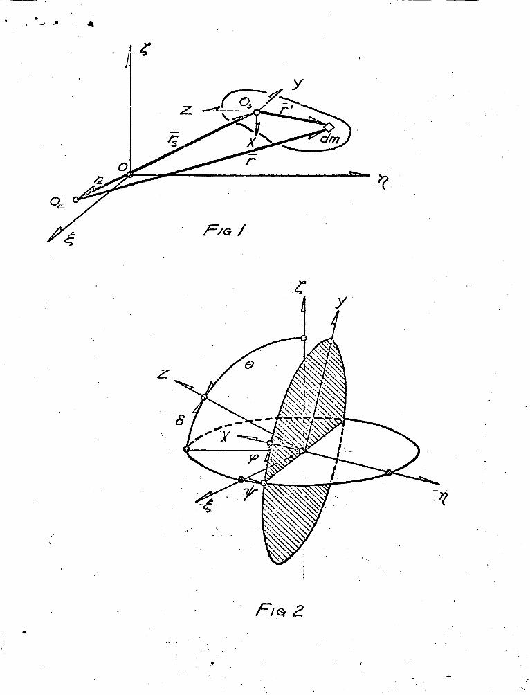
The basic equations of the satellite are established from the system

of position vectors shown in Fig. 1. Vector T- defines the distance between

center of m a s s OE of the earth and a particle in the satellite, YE the distance

between center of m a s s 0 of the whole system and center of m a s s OE of the

earth, TS the distance between center of m a s s 0 of the whole system and

center of mass 0, of the satellite, and ?'the distance between center of m a s s

Os of the satellite and a particle in the satellite. These vectors have com-

ponents in each of two different coordinate systems, one inertial and the

other body fixed. Inertial coordinates are 9 0 q I g with origin at 0 and

body fixed x,y,z with origin at 0,.

By representing masses of the earth and satellite by mE and ms

respectively, the following equations are readily established:

and

r n = m ~ + m s t' =r, - G = a c mti

where

The vector FA is the displacement between points 0 and Os. E The m a s s particle dm is attracted by gravitational forces and by

inner forces d 5. Using Newton's third law, &ere follows

9

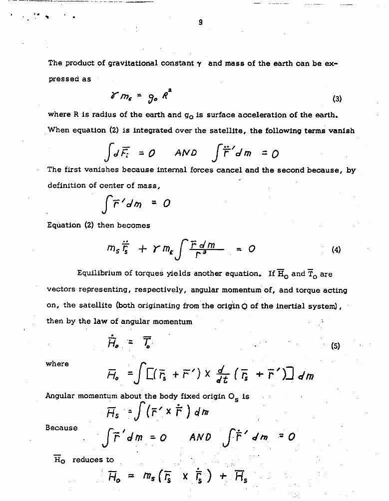
The product of gravitational constant 7 and mass of the earth can be ex-

pressed as

rm = 9. A= (3)

where R is radius of the earth and go is surface acceleration of the earth.

When equation (2) is integrated over the satellite, the following terms vanish

. The first vanishes because internal forces cancel and the second because, by

definition of center of mass ,

S F ' d m = 0

Equation (2) then becomes

Equilibrium of torques yields another equation. If zo and To are

vectors representing, respectively, angular momentum of, and torque acting

on, the satellite (both originating from the origin 0 of the inertial system),

then by the law of angular momentum

where

Angular momentum about the body f ixed origin Os is <

Rs 1

10

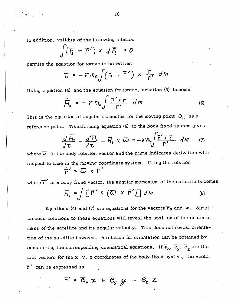
In addition, validity of the following relation n

permits the equation for torque to be written

Using equation (4) and the equation for torque, equation (5) become n

This is the equation of angular momentum for the moving point Os a s a

reference point. Transforming equation (6) to the body fixed system gives

where is the body rotation vector and the prime indicates derivation with

respect to t i m e in the moving coordinate system. Using the relation

?‘= a x F’ wherer’ is a body fixed vector, the angular momentum of the satellite becomes

Equations (4) and (7) are equations for the vectorsFs and z. Simul-

taneous solutions to these equations will reveal the position of the center of

mass of the satellite and its angular velocity. This does not reveal orienta-

tion of the satellite however. A relation for orientation can be obtained by

considering the corresponding kinematical equations. If Fx, 5 - eZ are the Y’

unit vectors for the x, y , z coordinates of the body fixed system, the vector

r can be expressed a s -/

+ + ez z

11

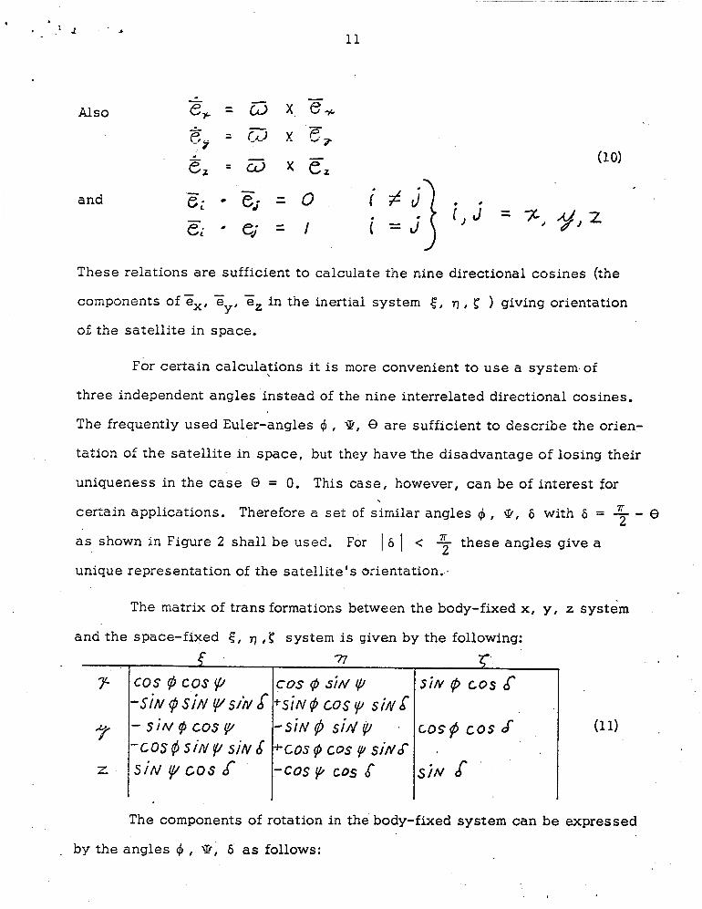
Also

and

These relations are sufficient to calculate the nine directional cosines (the -

components of ex. Z

of the satellite in space.

e, in the inertial system E , r ) , ) giving orientation Y'

For certain calculations it is more convenient to use a system,of

three independent angles instead of the nine interrelated directional cosines.

The frequently used Euler-angles C$ , Q, 0 are sufficient to describe the orien-

tation of the satellite in space, but they have t h e disadvantage of losing their

uniqueness in t h e case 8 = 0. Th i s case, however, can be of interest for

certain applications. Therefore a set of similar angles C$ , \k, 6 with 6 = - * e - 2 a s shown in Figure 2 shall be used. For 16 1 < 7 7r these angles give a

unique representation of the satellite's orientation. -

The matrix of trans formations between the body-fixed x, y, z system

and the space-fixed E f q ,p system is given by the following:

SiN 9 cos 6

cosp cos J

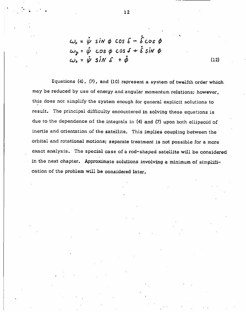
The components of rotation i n the body-fixed system can be expressed

. by the angles C$ , Q, 6 as follows:

12

4

#! = r; SiN @ cos 6- scos 9

Equations (4) (7) and (10) represent a system of -Nelfth order which

may be reduced by use of energy and angular momentum relations; however,

th i s does not simplify the system enough for general explicit solutions to

result. The principal difficulty encountered in solving these equations is

due to the dependence of the integrals in (4) and (7) upon both ellipsoid of

inertia and orientation of the satellite. This implies coupling between the

orbital and rotational motions; separate treatment is not possible for a more

exact analysis. The special case of a rod-shaped satellite will be considered

in the next chapter. Approximate solutions involving a minimum of simplifi-

cation of the problem will be considered later.

13

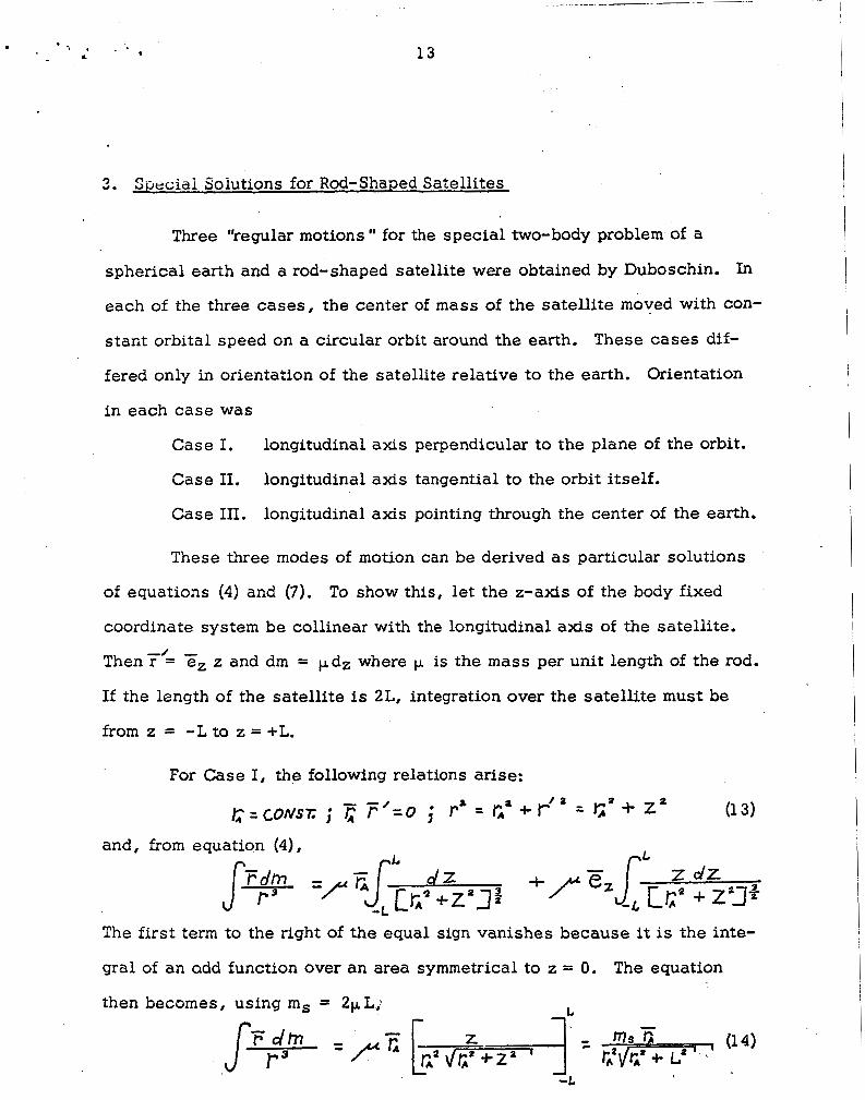
3. Sijeciai Soiutions for Rod-Shaped Satellites

Three "regular motions" for the special two-body problem of a

spherical earth and a rod-shaped satellite were obtained by Duboschin. In

each of the three cases, the center of m a s s of the satellite moved with con-

stant orbital speed on a circular orbit around the earth. These cases dif-

fered only in orientation of the satellite relative to the earth. Orientation

in each case was

Case I. longitudinal axis perpendicular to the plane of the orbit.

Case 11. longitudinal axis tangential to the orbit itself.

Case 111. longitudinal axis pointing through the center of the earth.

These three modes of motion can be derived as particular solutions

of equations (4) and (7).

coordinate system be collinear with the longitudinal axis of the satellite.

Then r = e, z and dm = pdz where p, is the m a s s per unit length of the rod.

If the length of the satellite is 2L, integration over the satellite must be

from z = -L to z = +L.

To show this, let the z-axis of the body fixed

-1 -

For Case I, the following relations arise:

(1 3) C = C ~ N S T ; ; - c -1 r =o ; r+ = t f + P = G' + 2'

and, from equation (4),

=/" r, Z t;' + z y

The f i rs t term to the right of the equal sign vanishes because it is the inte-

gral of an add function over an area symmetrical to z = 0. The equation

then becomes, using ms = 2pL; L -

-L

. . -. i . ' 14

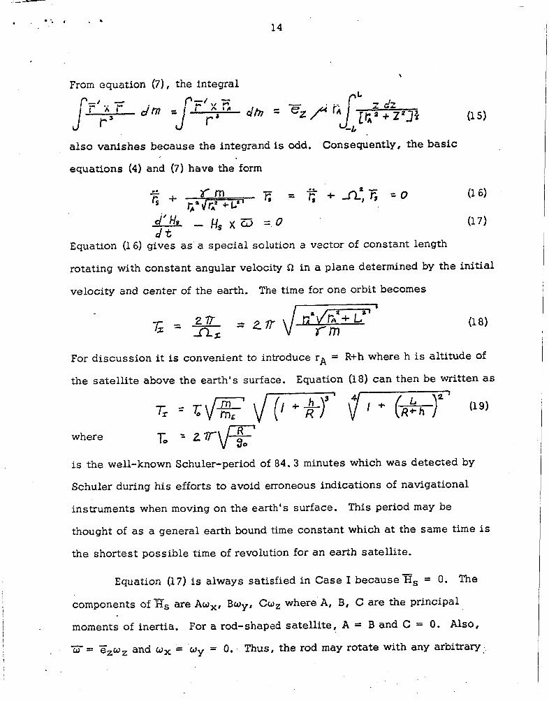
From equation (7), the integral

also vanishes because the integrand is odd. Consequently, the basic

equations (4) and (7) have the form

Equation (16) gives a s a special solution a vsctor of constant length

rotating with constant angular velocity fi in a plane determined by the initial

velocity and center of the earth. The t i m e for one orbit becomes

For discussion it is convenient to introduce rA = R+h where h is altitude of

the satellite above the earth's surface. Equation (18) can then be written as

where

is the well-known Schuler-period of 84.3 minutes which was detected by

Schuler during his efforts to avoid erroneous indications of navigational

instruments when moving on the earth's surface. This period may be

thought of as a general earth bound time constant which at the same t i m e is

the shortest possible t i m e of revolution for an earth satellite.

Equation (1 7) is always satisfied in Case I because xs = 0. The

components of gs are AwX, B o y , Co, where A, B, C are the principal

moments of inertia. ! For a rod-shapsd satellite, A = B and C = 0. Also,

I - - , o = ezuz and wx = wy = 0. Thus, the rod may rotate with any arbitrary

1

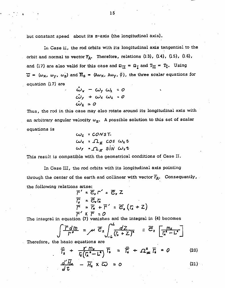
. - 15 7 . c

but constant speed about i t s z-axis (the longitudinal axis).

i ~ l Case i r , the rod orbits with its longitudinal axis tangential to the

orbit and normal to vector FA. Therefore 8 relations (1 3) 8 (14) 8 (1 5) 8 (1 6) 8

and (17) are also valid for this case and z211 = nI and TII = TI. Using

. equation (17) are Gt - wy w, = 0 cj, + c 3 x W z = o c;lr = o

Thus, the rod in this case may also rotate around its longitudinal axis with

an arbitrary angular velocity oz. A possible solution to t h i s set of scalar

equations is Cdz = CONST-

WJc = R, cos w,t W Y a n n siN uZt

This result is compatible with the geometrical conditions of Case 11.

In Case 111, the rod orbits with its longitudinal axis pointing

through the center of the earth and collinear with vector FA. Consequently,

the following relations arise: j=' = - e,r' = Ez z

j= F J & i" = o

= E +F' = E-(G + z ) The integral in equation (7) vanishes and the integral in (4) becomes

Therefore, the basic equations are

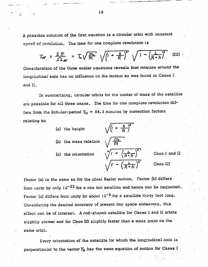
16

A possible solution of the first equation is a circular orbit with constant

speed cf rcvd i i th i i . Tie time for one complete revolution is

Consideration of the three scalar equations reveals that rotation around the

longitudinal axis has no influence on the motion a s was found in Cases I

and 11.

In summarizing, circular orbits for the center of mass of the satellite

are possible for a l l three cases. The t i m e for one complete revolution dif-

fers from the Schuler-period To = 84.3 minutes by correction factors

relating td:

(a) the height

(b) the mass relation

(c) the orientation Case I and I1

Factor (a) is the same as for the ideal Kepler motion. Factor (b) differs

from unity by only. 1 0-22 for a one ton satellite and hence can be neglected.

Factor (c) differs from unity by about

Considering the desired accuracy of present day space endeavors, this

effect can be of interest, A rod-shaped satellite for Cases I and I1 orbits

slightly slower and for Case I11 slightly faster than’a mass point on the

for a satellite thirty feet long.

. same orbit.

Every orientation of the satellite for which the longitudinal axis is

perpendicular to the vector 5 has the same equation of motion for Cases I . .

. . I

0 -

' . : 17

and 11. However, equation (17) has no soli tion which satisfies .he geome-

4 . d -- 9 U A ~ ~ ~ condiiions for the whole orbit -0 except for the special Cases I and 11.

Because the principal moment of inertia C Is zero, the vector of angular

momentum Rs is always perpendicular to the axis of the rod. Furthermore,

it is perpendicular toFA. For the satellite to have the same orientation

relative to the earth, must change its orientation i n space. This is pos-

sible if and only if a corresponding torque is present. However, this is not

the.case in equation (17).

8

.. .

. . . .

. . . . .

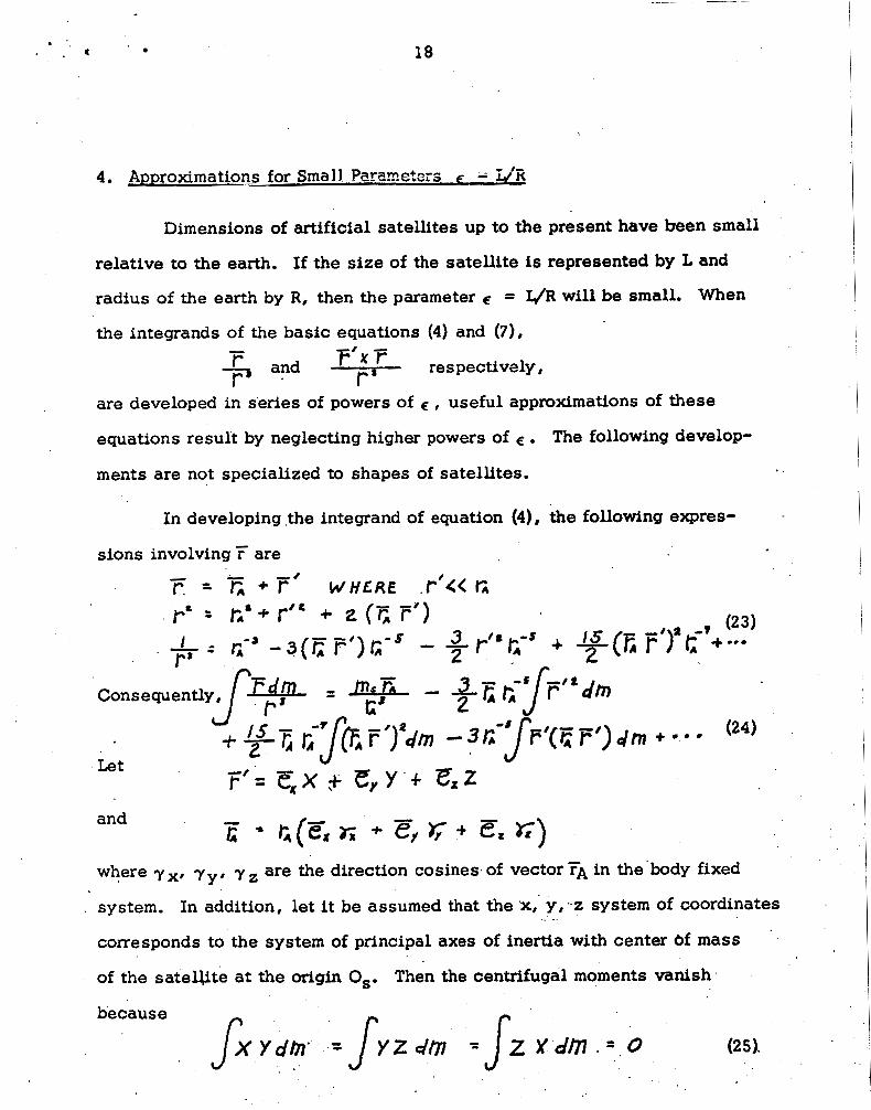
* . ' . 4 18

Dimensions of artificial satellites up to the present have been small

relative to the earth. If the size of the satellite is represented by L and

radius of the earth by R, then the parameter e: = I,/R will be small.

the integrands of the basic equations (4) and (7)#

When

respectively, F'x F r'

- and 7 .

are developed in series of powers of Q , useful approximations of these

equations result by neglecting higher powers of E: . ments are not specialized to shapes of satellites.

The following develop-

. .

In developing the integrand of equation (4), the following expres-

sions involving i are - - r. = r~ +F' W H E R E .t+< 6 P* = L*+ r'' + 2 (c F') (23)

Consequently,

(24)

- Let F'= exx ,c e y Y + e;z and

where yx, yy, y are the direction cosines of vector FA in the'body fixed

system. In addition, let it be assumed that the ZC, y,-z system of coordinates

corresponds to the system of principal axes of inertia with center bf m a s s

of the satelute at the origin Os. Then the centrifugal moments vanish

. .

f 19

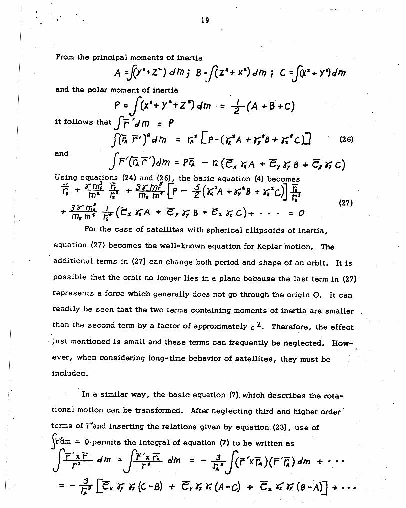
From the principal moments of inertia

A $Y .+zS) dm j 0 =JZ8 t X') dm ; C =J@'+Ys)dm and the polar moment of inertia

'+ Y'iZ*)dm . = r [ A ' .I. 8'+c)

and

equation (27) becomes the well-known equation for Kepler motion. The

additional terms in (27) can change both period and shape of an orbit. It is

possible that the orbit no longer lies i n a plane because the last term in (27)

represents a force which generally does not go through the origin 0. It can

readily be seen that the two terms containing moments of inertia are smaller. .

than the second te rm by a factor of approximately E 2. Therefore, the effect

just mentioned is s m a l l and these terms can frequently be neglected. How-

ever, when considering long-time behavior of satellites, they must be

included.

' In a similar way, the basic equation (7). which describes the rota-

tional motion can be transformed. After neglecting third and higher order

terms of ?and inserting the relations given by equation. (23) , use of

20

..- I

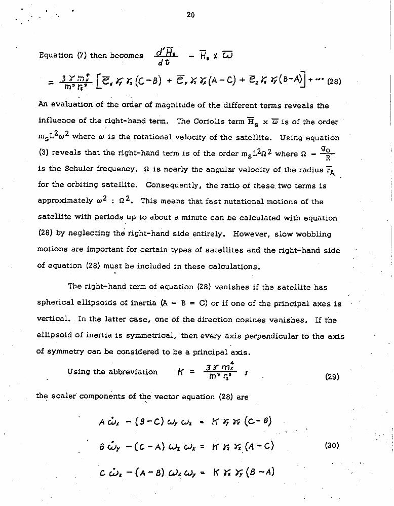
Equation (7) then becomes fi - H s x C 3 d t

An evaluation of the order of magnitude of the different terms reveals the

influence of the right-hand term. The Coriolis term Es x ?Z is of the order msL 2 2 w where w is the rotational velocity of the satellite. Using equation

(3) reveals that the right-hand term is of the order msL2522 where 52 = R g0 I

is the Schuler frequency. Q is nearly t h e angular velocity of the radius FA

for the orbiting satellite. Consequently, the ratio of these two terms is I

I

approximately a2 : Q2. This means that fast nutational motions of the I

I ~

, satellite with periods up to about a minute can be calculated with equation

(28) by neglecting the right-hand s ide entirely. However, slow wobbling

motions are important for certain types of satellites and the right-hand side

of equation (28) must be included in these calculations. . .

The right-hand term of equation (28) vanishes if the satell i te has

spherical ellipsoids of inertia (A = B = C) or i f one of the principal axes is

vertical. In the latter case, one of the direction cosines vanishes. If the

ellipsoid of inertia is symmetrical , then every axis perpendicular to the axis

of symmetry can be considered to be a principal axis.

1 3 r d m' 5' Using the abbreviation K =

the scaler'components of the vector equation (28) are -. I

. . .

- : ' - ' I . 21

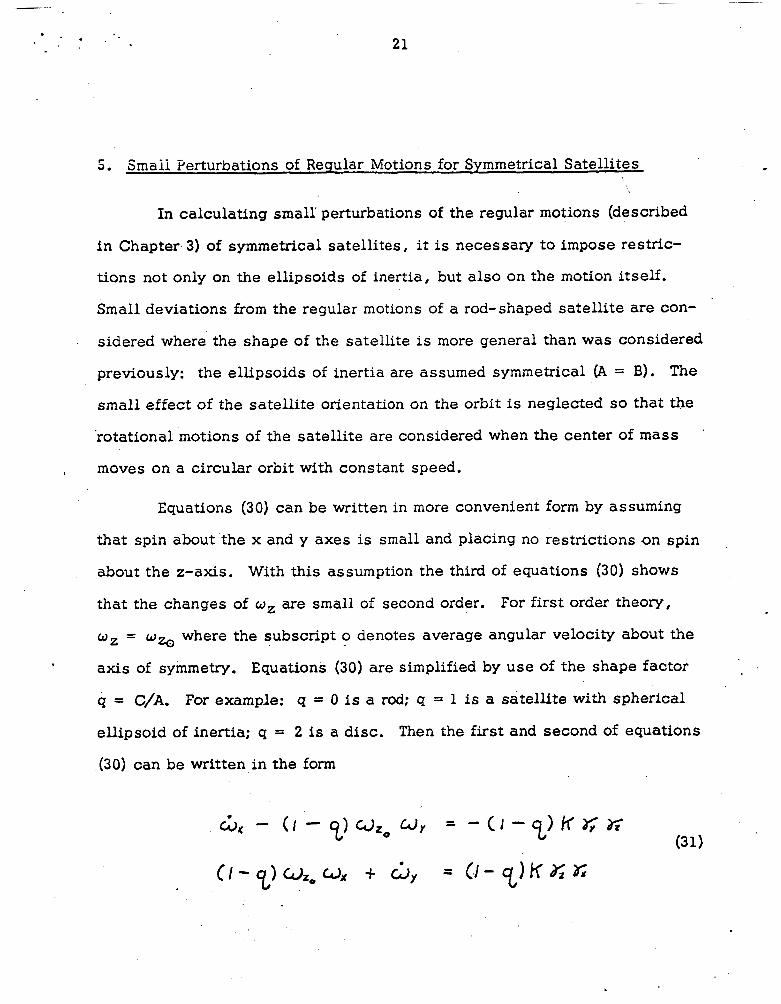
5. Smaii Perturbations of Reqular Motions for Symmetrical Satellites

In calculating small perturbations of the regular motions (described

i n Chapter 3) of symmetrical satellites, it is necessary to impose restric-

tions not only on the ellipsoids of inertia, but also on the motion itself.

Small deviations from the regular motions of a rod-shaped satellite are con-

sidered where the shape of the satellite is more general than was considered

previously: the ellipsoids of inertia are assumed symmetrical (A = B). The

small effect of the satellite orientation on the orbit is neglected so that the

'rotational motions of the satellite are considered when the center of mass

moves on a circular orbit with constant speed. ,

Equations (30) can be written in more convenient form by assuming

that spin about the x and y axes is small and placing no restrictions on spin

about the z-axis. With this assumption the third of equations (30) shows

that the changes of w z are small of second order. For first order theory,

oz = wzo where the subscript o denotes average angular velocity about the

axis of symmetry. Equations (30) are simplified by use of the shape factor

4 = C/A. For example: q = 0 is a rod; q = 1 is a satellite with spherical

.

ellipsoid of inertia; q = 2 is a disc. Then the first and second of equations

(30) can be written in the form

. r , *

, 8 . 22

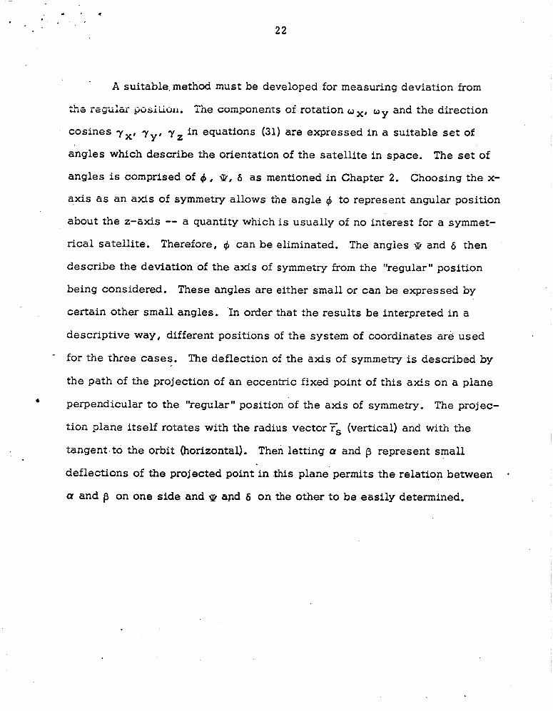
A sui-able. method mus be developed for measur,ng deviation from

&I- -_ -._ 7 -- u A ~ A F ; y U A a l Qjosiucjn. The componenrs of rotation w x, oY and the direction

cosines 7x8 7 y 8 7 , in equations (31) are expressed i n a suitable se t of

angles which describe the orientation of the satellite in space. The set of

angles is comprised of 6 8 a, 6 as mentioned in Chapter 2. Choosing the x-

axis a s an axis of symmetry allows t h e angle 4 to represent angular position

about the z-axis -- a quantity which is usually of no interest for a symmet-

rical satellite. Therefore, 4 can be eliminated. The angles Q and 6 then

describe the deviation of the axis of symmetry from the "regular" position

being considered. These angles are either small or can be expressed by

certain other small angles. In order that the results be interpreted in a

descriptive way, different positions of the system of coordinates are used

for the three cases. The deflection of the axis of symmetry is described by

the path of the projection of an eccentric fixed point of this axis on a plane

perpendicular to the "regular" position of the axis of symmetry. The projec-

tion plane itself rotates with the radius vector Ts (vertical) and with the

tangent. to the orbit (horizontal). Then letting cy and p represent small

deflections of the projected point in this plane permits the relation between

cy and p on one side and

*

and 6 on the other to be easily determined.

. - - ' . 23

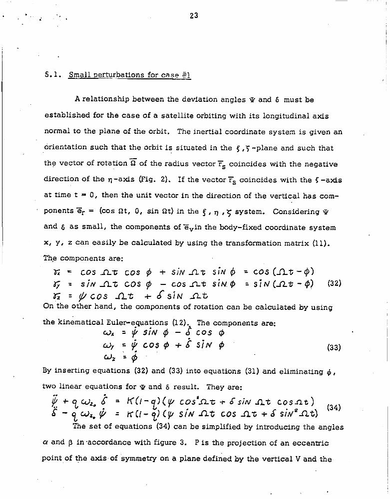
5.1. Small perturbations for case 81

A relationship between the deviation angles Q? and 6 must be

established for the case of a satellite orbiting with its longitudinal axis

normal to the plane of the orbit. The inertial coordinate system is given an

orientation such that the orbit is situated in the 5 8 5 -plane and such that

the vector of rotation 5 of the radius vector is coincides with the negative

direction of the q -axis (Fig. 2). If the vector Fs coincides with the C -axis

at t i m e t = 0, then the unit vector in the direction of the vertical has cam-

' ponents Zr = (COS at, 0, sin a t ) in the 5 , 11 ,5 system. Considering Q

and 6 as sma l l , the components of Zvin the body-fixed coordinate system

x, y8 z can easily be calculated by using the transformation ma t r ix (1 1).

The components are:

x = cos a-t; COS 9 + s i r / A t S ~ N 4 = cos ( f i t -@> q = s h n t cos p - c o s n t s i N @ = s i n l ( n t - 4 ) (32) i~ = p c o s fit -i- J s i ~ fit

On the other hand, the components of rotation can be calculated by using

the kinematical Euler-equations (1 2) .- The components are: 0 s = $b 5iN @ - 6 cos @ W, = y COS + 2 s i N p G1, = 8 (3 3)

By inserting equations (32) and (33) into equations (31) and eliminating 4 ,

two linear equations for Q? and d result. They are:

(34) $j + T u z e t = K ( I - % ) ( ~ cos 'n t t J s i M fit c o s n t ) 6 - y4 + = K C I - ~ I QU s h nt COS n.-t + d siu2fit)

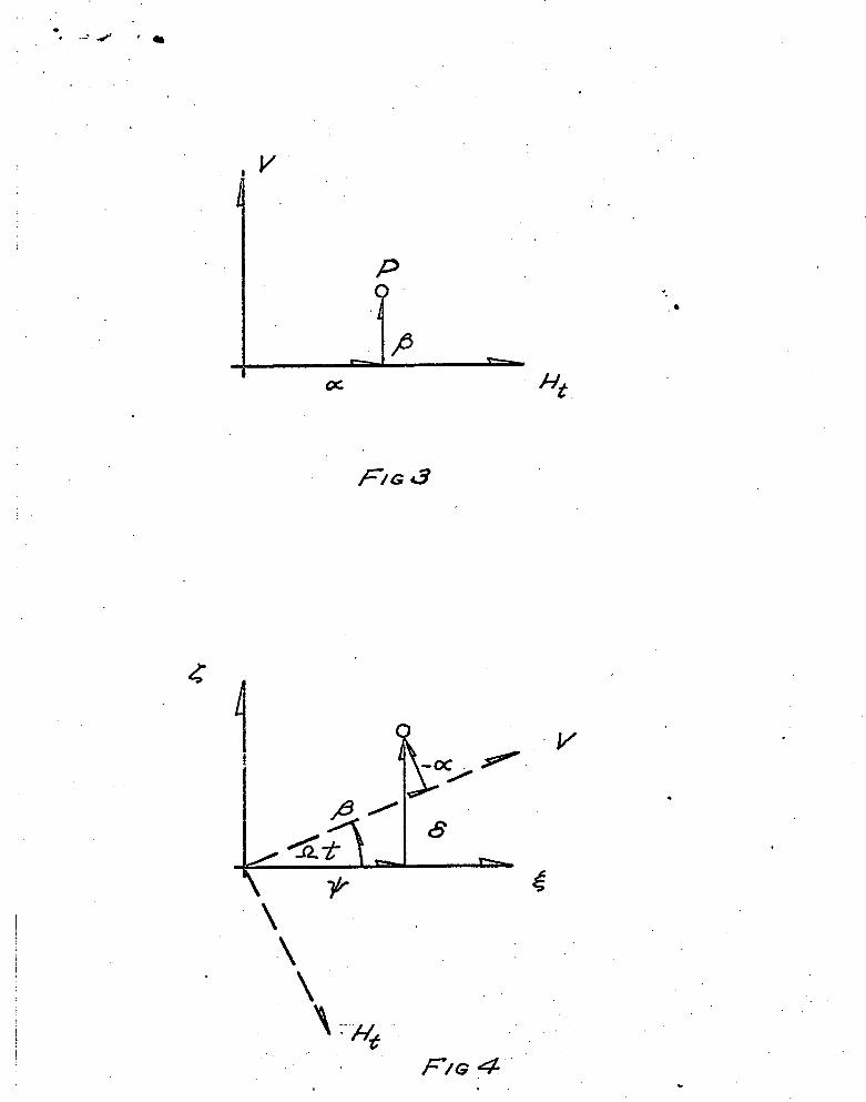
The set of equations (34) can be simplified by introducing the angles

CY and p in -accordance with figure 3. P is the projection of an eccentric

point of the axis of symmetry on a plane defined by the vertical V and the

. * . 24

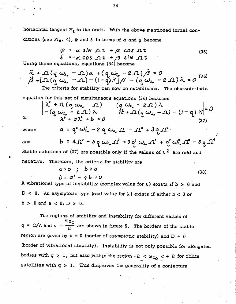
horizontal tangent Ht to the orbit. With the above mentioned initial con-

ditions (see Fig. 4), * and 6 in terms of a and p become

$b = a s i l v nt +/3 c o s f i t d cos nt + p s i N fit

Using these equations, equations (34) become

(35)

The criteria for stability can now be established. The characteristic

equation for this set of simultaneous equations (36) becomes 7c + n ( q w z o - a ) ( ~ " . - 2 R ) A -(q,wz, - 2 J l ) h 7ca + n (? or, -n> - ( I - q,)

. (37) or h 4 + d + b 5 0

Stable solutions of (37) are possible only if the values of X

negative. Therefore , the criteria for stability are

are real and

A vibrational type of instability (complex value for A ) exists if b > 0 and

D 0. . A n asymptotic type (real value for A ) exists if either b e 0 or

b > O a n d a O;D > 0.

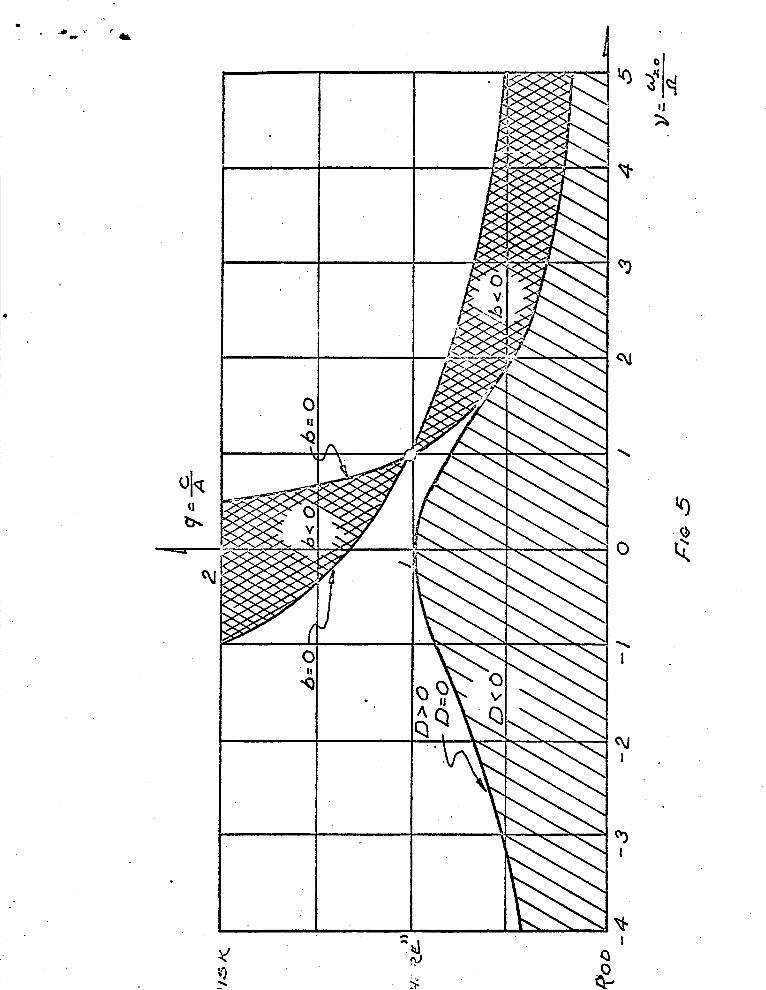
The regions of stability and instability for different values of

are shown in figure 5. The borders of the stable +O q = C/A and u =

region are given by b = 0 (border of asymptotic stability) and D = 0

(border of vibrational stability). Instability is not only possible for elongated

bodies with q > 1 , but also .within the-reginn -52 i: oz0 + $2 for oblite I - - - .

satellites with q > 1. This disproves the generality of a conjecture

I . . . .i

8

mentioned by Duboschin. In summarizing the results of his calculations,

he stated that the stability-properties of rod-shaped and disc-shaped

satellites are direct oppo.qite, meaning t ! !zt the disc-shapea sateiiite is

stable where the rod-shaped satellite is unstable and vice versa. As an

example, consider the case I for o = 0 where both types are unstable.

Only slightly oblated satellites with 1 c q c 1.33 can be used in this case 20

without spin. The situation can be improved by a spin w

frequency s1. For this case all types of oblate symmetrical satellites are

equal to orbital 20

stable.

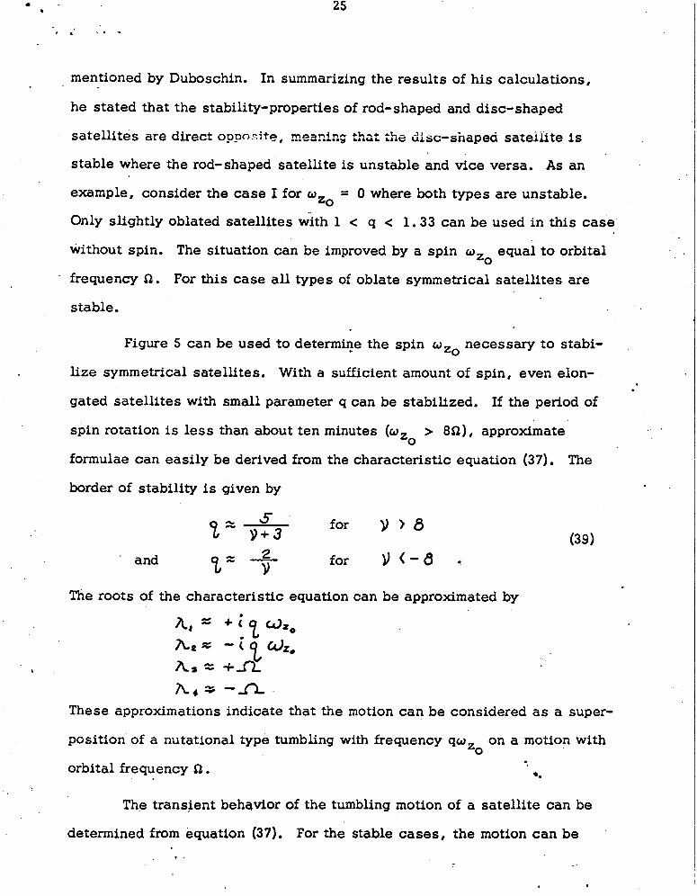
Figure 5 can be used to determine the spin wzo necessary to stabi- .

lize symmetrical satellites. With a sufficient amount of spin, even elon-

gated satellites with s m a l l parameter q can be stabilized. If the period of

spin rotation is less than about ten minutes (w

formulae can easily be derived from the characteristic equation (37). The

> 8521, approximate zO

border of stability is given by

and for 3 (-6 (39)

The roots of the characteristic equation can be approximated by

A , = + i , c 3 z , ha= - icpe A , = +,R.

I l 4 s - n

These approximations indicate tha t the motion can be considered as a super-

position of a nutational type tumbling with frequency qw on a motion with ZO

orbital frequency s1. .. The trans4ent behavior of the tumbling motion of a satellite can be

determined from equation (37). For the stable cases, the motion can be

26

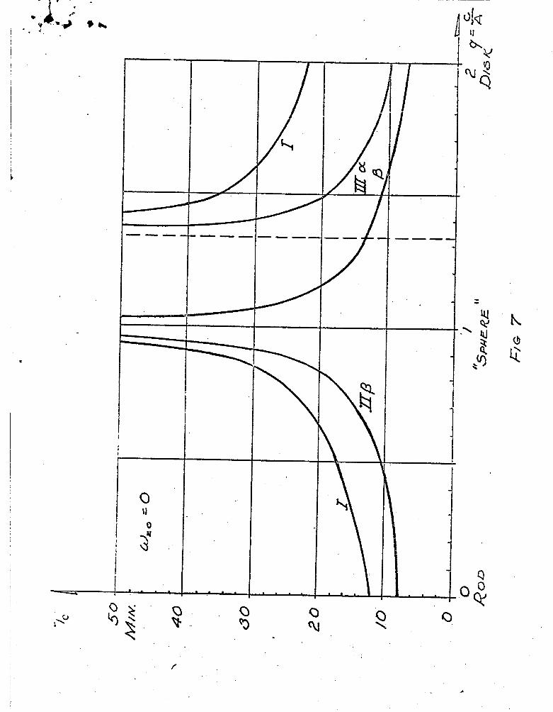
. characterized by the frequency-ratio n = # ; for the unstable cases, the 1 amount of instability can be determined by the t ime constant Tc = Far"L of

During the t ime T,, the deflection increases by a factor e = 2.718. Dia-

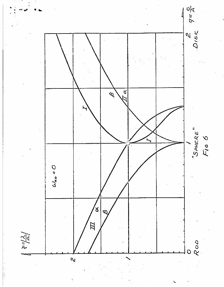
g rams of n and T, for the three cases considered herein are shown in figures

6 and 7. Both diagrams are valid for non-spinning satellites (w = 0). 20

For case I, the possible modes of motion are equally valid for both

angles a and p . Thus the curve in figure 6 corresponding to case I is simply

denoted by "I". When two frequencies exist (for 1 f q 5 1.333) , the

motion is stable. One of the frequencies is smaller and the other one

greater than the orbital frequency which is characterized by n = 1.

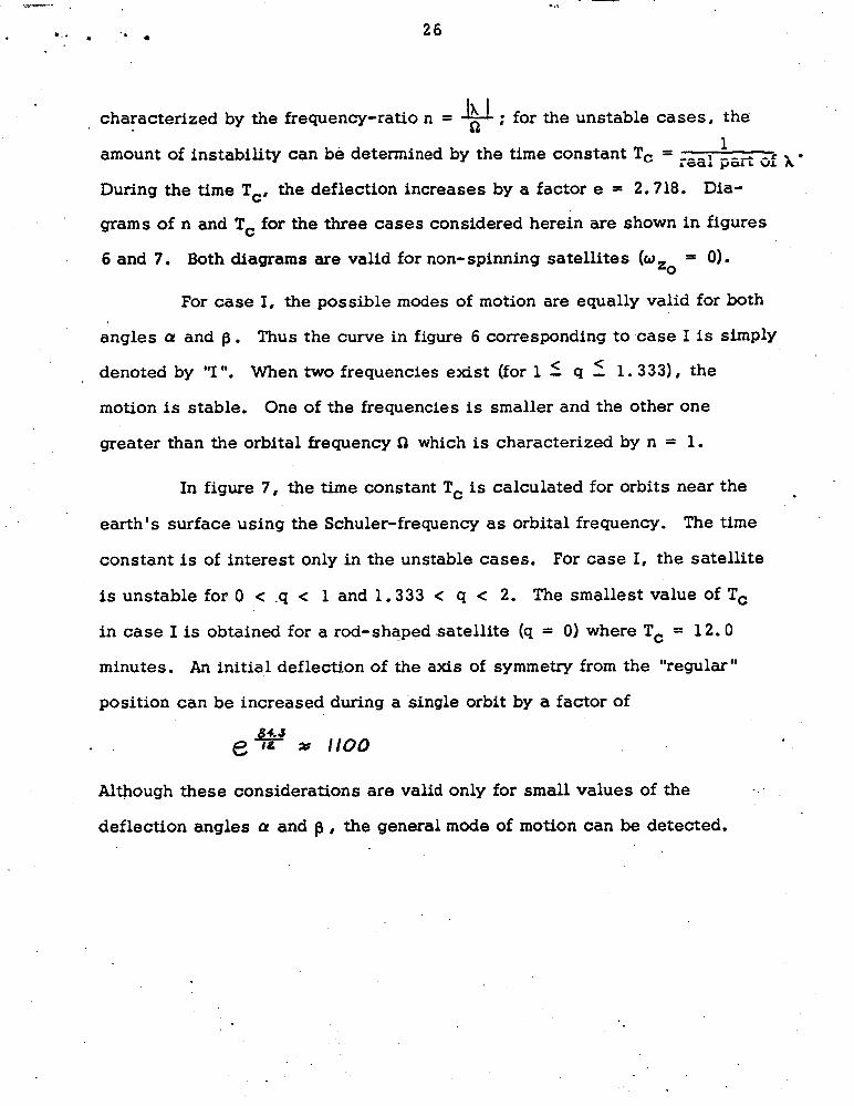
In figure 7, the t i m e constant Tc is calculated for orbits near the

earth's surface using the Schuler-frequency as orbital frequency. The t i m e

constant is of interest only in the unstable cases. For case I, the satellite

is unstable for 0 < .q c 1 and 1.333 e q < 2. The smallest value of Tc

in case I is obtained for a rod-shaped satellite (q = 0) where Tc = 12.0

minutes. An initial deflection of the axis of symmetry from the "regular"

position can be increased during a single orbit by a factor of

- .

Although these considerations are valid only for sma l l values of the

deflection angles a and p , the general mode of motion can be detected.

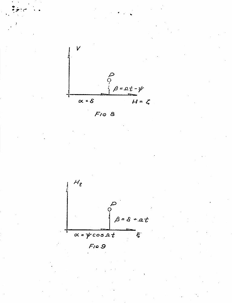
FIG 8

27

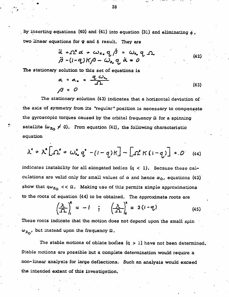
5 . 2 Small perturbations for the case I1

A relationship between thedeviation angles Q and 6 must be

established for the case of a satellite orbiting with its axis of symmetry

tangent to the orbit. The inertial coordinate system is given an orLentation

such that the orbit is situated in the f , 5 -plane (Fig. 2). The undisturbed

orientation of the satellite is given by qj = at and 6 = 0. If the.deviations

from these values are assumed s m a l l , then the variables

A = b A N D p = n t - y will also be small . Once again these angles indicate the deflection of the

axis of symmetry from the undisturbed position. This deflection can be

represented by the projection of a point eccentric to the axis of symmetry on

a plane comprised of the vertical direction and the horizontal 5 -axis (see

fig. 8). If TS coincides with the negative < -direction at t i m e t = 0, then

. the components of FV in the c , q , 9 system are

L e, = ( -COS n f , - S ~ N nt, 0 1 SI::e a! and are s m a l l angles, the corresponding components in the x, y, -

z system are -

(40) e, =: ( - c o s d l si4v

The components of rotation from equation (12) become

w* = a s;N # - k cos p - p SiN #

* * , ?

~~ ~ _. . ... . . . . . . . - , - . . . . . . -.. 28

. .

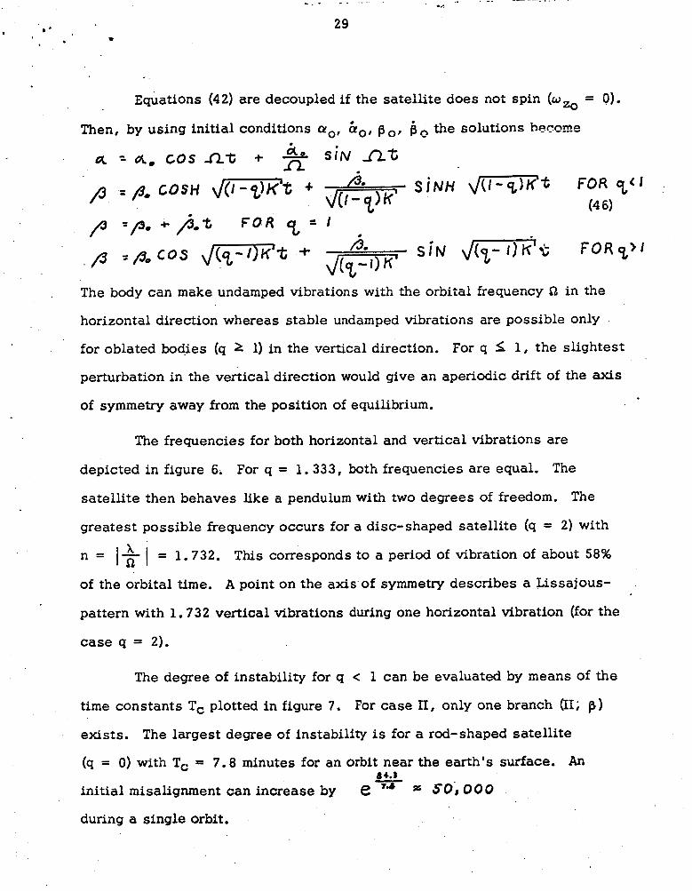
By inserting equations (40) and (41) into equation (31) and eliminating t$ 8

two.linear equations for Q and 6 result. They are

The stationary solution to this set of equations is % 0% n (43)

A =oc. =

/ 3 = 0 The stationary solution (43) indicates that a horizontal deviation of

the axis of symmetry from its "regular" position is necessary to compensate

the gyroscopic torques caused by the orbital frequency 42 for a spinning m.

satellite bz0 # 0). From equation (42), the following characteristic

equation

indicates instability for a l l elongated bodies (q c 1). Because these cal-

culations are valid only for s m a l l values of Q! and hence cyo8 equations (43)

show that qwzo << S i . Making use of th is permits simple approximations

. to the roots of equation (44) to be obtained. The approximate roots are

These roots indicate that the motion does not depend upon the s m a l l spin

o but instead upon the frequency 52. 20

The stable motions of oblate bodies (q > 1) have not been determined.

Stable motions are possible but a complete determination would require a

non-linear analysis for large deflections. Such an analysis would exceed

the intended extent of this investigation.

, 0 ’ 1

w

Equations (42) are decoupled i f the satellite does not spin (wzo = 0).

Then, by using initial conditions CY,, h0, pol b , the solutions hemme

4 = A , cos + i~ sinr nt A

The body can make undamped vibrations with the orbital frequency Q in the

horizontal direction whereas stable undamped vibrations are possible only

for oblated bodies (q 2 1) in the vertical direction. For q I 1, the slightest

perturbation in the vertical direction would give an aperiodic drift of the axis

of symmetry away from the position of equilibrium.

The frequencies for both horizontal and vertical vibrations are

depicted in figure 6. For q = 1.333, both frequencies are equal. The

satellite then behaves like a pendulum with two degrees of freedom. The

greatest possible frequency occurs for a disc-shaped satellite (q = 2) with

n = 1~ I = 1.732. This corresponds to a period of vibration of about 58% x

of the orbital time. A point on the axis of symmetry describes a Lissajous-

pattern with 1.732 vertical vibrations during one horizontal vibration (for the

case q = 2).

The degree of instability for q < 1 can be evaluated by means of the

t i m e constants T, plotted in figure 7. For case 11, only one branch (II; p)

exists. The largest degree of instability is for a rod-shaped satellite

(q = 0) with T, = 7.8 minutes for an orbit near the earth’s surface. An

initial misalignment can increase by e ‘4 1: 5 0 , 0 0 0

during a single orbit.

8 4.3 -

_. .--

. ' * % . ' . 30

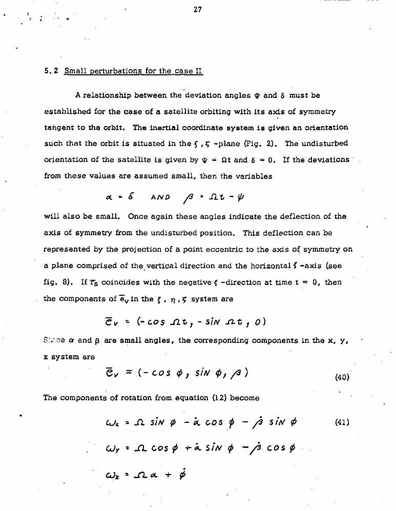
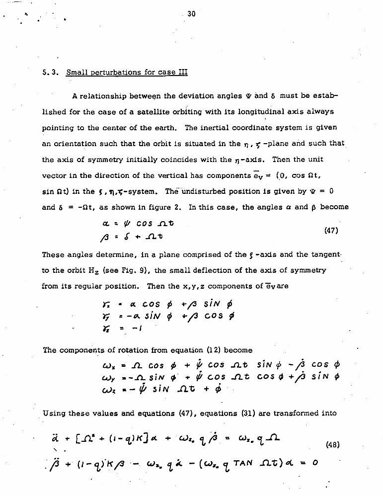
5.3. Small perturbations for case I11

A relationship between the deviation angles ip and 6 must be estab-

lished for the case of a satellite orbiting with its longitudinal axis always

pointing to the center of the earth. The inertial coordinate system is given

an orientation such that the orbit is situated in the , f -plane and such that

the axis of symmetry initially coincides with the q-axis. Then the unit

vector i n the direction of the vertical has components &, = ( 0 , cos at, s in h t ) in the S 8 q,y-system. The- undisturbed position is given by ip = 0

and 6 = -r(2t# as shown in figure 2. In this case, the angles a! and 8 become

These angles determine, in a plane comprised of the 5 -axis and the tangent-

to the orbit H, (see Fig. 9'), the s m a l l deflection of the axis of symmetry

from its regular position.. Then the x, y , z components of Zvare

The components of rotation from equation (12) become

w X = n COS + + t COS nt s i N 9 -/j C O S

0, = - n s i n r 9' + + cos nt COS 0 +/j S i N 9 ~ 1 3 ~ = - $ sir\ l nt + 6

Using these values and equations (47), equations (31) are transformed into

'L - W z o 4, T A N rrt) 4 0

31

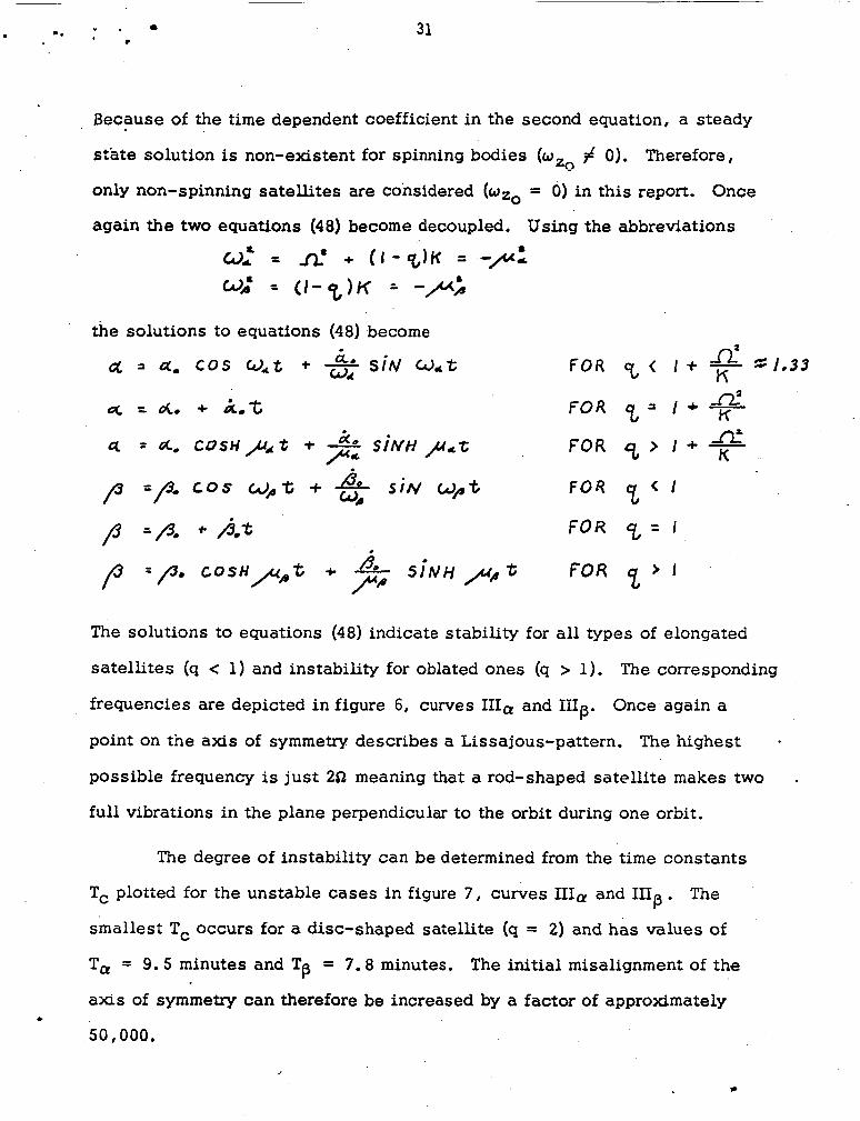
Because of the t i m e dependent coefficient in the second equation, a steady

state solution is non-existent for spinning bodies (w

only non-spinning satellites are considered (wzo = 0) in this report. Once

again the two equations (48) become decoupled. Using the abbreviations

# 0). Therefore, 20

a o,L = fi8 + ( 1 - q ) ~ = -pd G$ = ( l - % ) K = -/c.ifb

the solutions to equations (48) become

The solutions to equations (48) indicate stability for all types of elongated

satellites (q c 1) and instability for oblated ones (q > 1). The corresponding

frequencies are depicted in figure 6, curves IIIa and 111~. Once again a

point on the axis of symmetry describes a Lissajous-pattern. The highest *

possible frequency is just 20 meaning that a rod-shaped satell i te makes two -

full vibrations in the plane perpendicular to the orbit during one orbit.

The degree of instability can be determined from the t i m e constants

Tc plotted for the unstable cases in figure 7 , curves IIIa and IIIp. The

smallest Tc occurs for a disc-shaped satellite (q = 2) and has values of

T, = 9.5 minutes and Tp = 7.8 minutes. The initial misalignment of the

a ~ s of symmetry can therefore be increased by a factor of approximately

50,000.

32

It is remarkable that the periods of vibration and the t i m e oonstants

are nearly independent of length of the satellite. The influence of the s ize . 8 - \ z

of the satell i te is of the order (k) For approximate calculation, this

effect can be fully neglected. This shows that, even for very small satellites,

the surrounding gravity field cannot be considered homogeneous when long

periodic rotational motions are of interest.

c

6. Results

33

The direction of the gravity force acting on a finite body in a radial

gravity field does not generally pass through the center of mass of that body. ~

This results in (1) a torque about the center of m a s s and (2) a non-central i component of the force. These conditions produce a coupling between the 1

orbital and rotational motions; hence, the equations of motion must be treated

simultaneously. Both equations cannot be treated separately as is usually

done in the classical problems of celestial mechanics. The equations of

motion are derived in detail in this report using the restrictions mentioned in

the first chapter. These equations, together with the kinematical equations

necessary to describe the orientation of the satellite in space, constitute a

system of differential equations of twelfth order.

Three partial1 solutions for the exact equations, previously mentioned

by Duboschin, are treated more in detail. These partial solutions show the

effects of orientation of the axis of symmetry upon the period of circular orbits.

In addition to the well-knokn corrections for the relation between masses of

the earth and satellite and for the distance of the orbit from the earth's surface,

a third correction is necessary to consider the orientation of a satellite in

orbit. In the case of a rod-shaped satellite for instance, the orbiting t i m e is

less i f the axis of the rod always points toward the center of the earth than it

is i f the axis is always tangential to the orbit. The center of masses in both

cases will have identical circular orbits . A series development of the basic equations (4) and (7) in terms of

L the ratio R (length of the satellite to radius of the earth) shows that the

. & d ..

34

infl.uence of satellite orientation upon the orbital motion is of second order

and hence smal l . This causes a non Keplerian motion with a slightly altered

period of revolution and also a certain deformation of the orbit. Orbits not

situated in a plane are possible. The development in power series shows

furthermore’that the gravity gradient torques must be taken into account if

slow tumbling motions are of interest. Tumbling is considered slow when the

period is of the order of magnitude of the orbiting period. For nutational motion

of spinning satellites, however, calculations by means of the classical Euler-

equations (which neglect gravity-gradient torques) are usually sufficiently

accurate . An analysis of the disturbed motions of symmetrical satellites shows

the possible types of motion and their stability. Symmetrical satellites .with

an orientation of the axis of symmetry perpendicular to the plane of the orbit

can be stabilized by introducing a spin around the axis of symmetry. The .

necessary value of spin depends upon the ratio of the principal moments of

inertia. Satellites without spin are in this case stable only for a s m a l l range

1 < q < 1.33, meaning only for slightly oblated satellites. In contradiction

to a statement by Duboschin, the rod-shaped and disc-shaped satellites are . unstable in this particular case. In case of a symmetr ica l satellite with the

axis of symmetry tangential to the orbit or deflecting only slightly from this

position, stable motions are possible for oblate bodies (q > 1). If, however,

>

the axis of symmetry points to the center of the earth, only elongated bodies

can give stable steady-state motions in a circular orbit.

The frequencies of possible vibrations are plotted versus shape-factor

q = C/A in’ fig. 6 for the stable configurations; t i m e constants T, are plotted

versus shape-factor q in fig. 7 for the unstable configurations. The t i m e

. * rp. ' - * 35

constant is a suitable measure of the degree of instability: within a period

of t i m e Tc, an initial misalignment of the axis of symmetry is increased by a

factor e = 2.718. For the more severe cases, the t i m e constant is so s m a l l

e

. that an initial error may be increased by a factor of approximately 50,000 in

a single orbit. For these cases, however, the linear analysis performed in

this investigation is insufficient for evaluation of the motion in question over

a longer time.

A remarkable result is that the transient behavior of disturbed satellites,

characterized by the frequency and time constant curves of figs. 6 and 7 respec-

tively, is nearly independent of the size of the satellite. This indicates that

even for very small satellites of perhaps no more than an inch in length, the

gravity-field cannot be considered homogeneous. Neglecting the radial prop-

erties of the gravity field would result io a loss of the effects mentioned here.

36

References

i. fi. E. iioberson, "Gravitational Torque on a Satellite Vehicle", J. Frankl. ' Ins t . , Vol. 265, No. 1, 1958, pp. 13-22.

, 2. R. E. Roberson, "A Unified Analytical Description of Satellite Attitude Motions", Astronautica Acta, Vol. V, 1959, pp. 347-355.

3. A. I. Lurje, "Some Problems of the Dynamics of Rigid Body Systems" (in Russian) , Trudi Leningradskovo Politchniceskovo Instituta, 1960, pp. 7-22.

4. Go N. Duboschin, "On the Differentiai Equations for the Orbital and Ro- tational Motions of Rigid Bodies Attracted by Gravitational Forces 'I (in Russian) Astramniceski Journal 35, 1958.

5. G. N. Duboschin, "On a Special Case of Orbital and Rotaticzai Motions of Two Bodies (in Russian), Astronomiceski Journal 3 6 , 1953, pp. 153-163.

6. G. N. Duboschin, "On the Rotational Motions of Artificial Celestial Bodies" (in Russian), Buletin Instituta Teoreticeskoi Astronomii VII, 1960, pp. 511-520.

7. W. R. Davis, "Determination of a Unique Attitude for an Earth Satellite", Proc. Amer. Astronautical Society, 4th Annual Meeting - Jan. 1958, pp. 10.1 - 10.15.

' 8. T. A. J. Stocker and R. F. Vachino, "The Two-Dimensional Librations of a .Dumbbell-Shaped Satellite in a Uniform Gravitational Field", Proc. Amer. Astronaurical Society, 1958, pp. 37.1 - 37.20.

9. J. H. Suddath, "A Theoretical Study of the Angular Motions of Spinning Bodies in Space", Tech. Report R-83, Langley Research Center, Langley Field, Va. , 1961, 12 pp.

10. R. G. Dole, M. E. Ekstrand, and M. R. O'Neill, "Motion of a Rotating Body - A Mathematical Introduction to Satellite Attitude Control", NAVWEPS Report 7619, 1961, China Lake, Calif.

11 . W. 5 . Xlemperer, "Satellite Librations of Large Amplitudes ' I , AFG - Journal Vol. 3 0 , 1960, pp. 123.

12. V. V. Beletskiy, "The Libration of a Satellite", Iskusstvennyye Sputniki Z e d i No. 3, 1959, pp. 13-31.

13. W. T. Thomson, "Spin Stabilization of Attitude Against Gravity Torque", J. Astronautical Sci. Vol. IX, 1962, pp. 31-33.

14. D. B.. DeBra, "The Large Attitude Motions and Stability, due to Gravity, '

of a Satellite with Passive Damping in an Orbit of Arbitrary Eccentricity about a n Oblate Body", Stanford University, SNDMR No. 126, May 1962.

Z

. . .

I . .

.

\ \ \

cs “ . I I

Q

7- \

0 I1

3" 0

\

1

h

Q

0

I

I

- f’ -. -

-

T ----

I. -I-/ I