Rough solutions of the Stochastic Navier-Stokes Equation · Rough solutions of the Stochastic Navier-Stokes Equation Björn Birnir Center for Complex and Nonlinear Science Department

Turbulence

Birnir

TheStochasticClosure ofNavier-Stokes

TheKolmogorov-Obukhov-She-LevequeScaling

The variabledensity windtunnel

Fitting thedata

The Error inthe Fit

Existence ofRoughSolutions

Conclusions

Rough solutions of the StochasticNavier-Stokes Equation

Björn Birnir

Center for Complex and Nonlinear ScienceDepartment of Mathematics, UC Santa Barbara

andUniversity of Iceland, Reykjavík

RICAM, Linz, December 2016

Co-authors, Gregory Bewley, Cornell, Michael Sinhuber, Göttingen, JohnKaminsky and Shahab Karmini, UC Santa Barbara

Turbulence

Birnir




Fitting thedata

The Error inthe Fit


Conclusions

Outline

1 The Stochastic Closure of Navier-Stokes

2 The Kolmogorov-Obukhov-She-Leveque Scaling

3 The variable density wind tunnel

4 Fitting the data

5 The Error in the Fit

6 Existence of Rough Solutions

7 Conclusions

Turbulence

Birnir




Fitting thedata

The Error inthe Fit


Conclusions

Outline




4 Fitting the data



7 Conclusions

Turbulence

Birnir




Fitting thedata

The Error inthe Fit


Conclusions

The Deterministic Navier-Stokes Equations

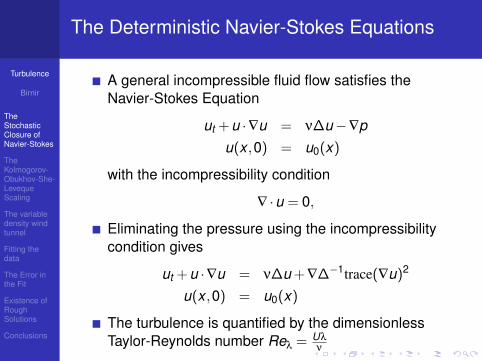
A general incompressible fluid flow satisfies theNavier-Stokes Equation

ut + u ·∇u = ν∆u−∇pu(x ,0) = u0(x)

with the incompressibility condition

∇ ·u = 0,

Eliminating the pressure using the incompressibilitycondition gives

ut + u ·∇u = ν∆u + ∇∆−1trace(∇u)2

u(x ,0) = u0(x)

The turbulence is quantified by the dimensionlessTaylor-Reynolds number Reλ = Uλ

ν

Turbulence

Birnir




Fitting thedata

The Error inthe Fit


Conclusions

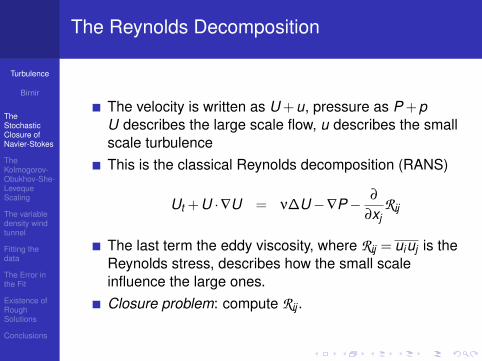
The Reynolds Decomposition

The velocity is written as U + u, pressure as P + pU describes the large scale flow, u describes the smallscale turbulenceThis is the classical Reynolds decomposition (RANS)

Ut + U ·∇U = ν∆U−∇P− ∂

∂xjRij

The last term the eddy viscosity, where Rij = uiuj is theReynolds stress, describes how the small scaleinfluence the large ones.Closure problem: compute Rij .

Turbulence

Birnir




Fitting thedata

The Error inthe Fit


Conclusions

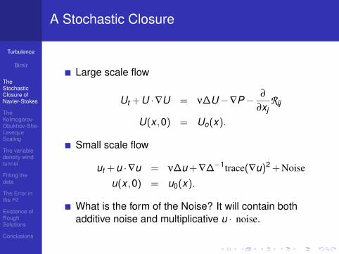
A Stochastic Closure

Large scale flow

Ut + U ·∇U = ν∆U−∇P− ∂

∂xjRij

U(x ,0) = Uo(x).

Small scale flow

ut + u ·∇u = ν∆u + ∇∆−1trace(∇u)2 + Noise

u(x ,0) = u0(x).

What is the form of the Noise? It will contain bothadditive noise and multiplicative u · noise.

Turbulence

Birnir




Fitting thedata

The Error inthe Fit


Conclusions

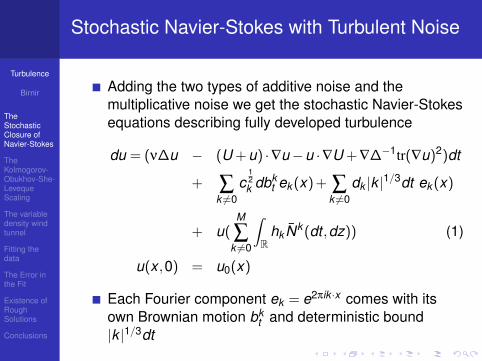
Stochastic Navier-Stokes with Turbulent Noise

Adding the two types of additive noise and themultiplicative noise we get the stochastic Navier-Stokesequations describing fully developed turbulence

du = (ν∆u − (U + u) ·∇u−u ·∇U + ∇∆−1tr(∇u)2)dt

+ ∑k 6=0

c12k dbk

t ek (x) + ∑k 6=0

dk |k |1/3dt ek (x)

+ u(M

∑k 6=0

∫R

hk Nk (dt ,dz)) (1)

u(x ,0) = u0(x)

Each Fourier component ek = e2πik ·x comes with itsown Brownian motion bk

t and deterministic bound|k |1/3dt

Turbulence

Birnir




Fitting thedata

The Error inthe Fit


Conclusions

Outline




4 Fitting the data



7 Conclusions

Turbulence

Birnir




Fitting thedata

The Error inthe Fit


Conclusions

The Kolmogorov-Obukhov Theory

In 1941 Kolmogorov and Obukhov [7, 6, 9] proposed astatistical theory of turbulenceThe structure functions of the velocity differences of aturbulent fluid, should scale with the distance (lagvariable) l between them, to the power p/3

E(|u(x , t)−u(x + l , t)|p) = Sp = Cplp/3

A. Kolmogorov A. Obukhov

Turbulence

Birnir




Fitting thedata

The Error inthe Fit


Conclusions

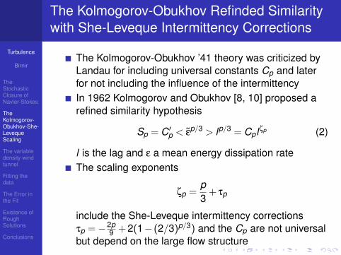
The Kolmogorov-Obukhov Refinded Similaritywith She-Leveque Intermittency Corrections

The Kolmogorov-Obukhov ’41 theory was criticized byLandau for including universal constants Cp and laterfor not including the influence of the intermittencyIn 1962 Kolmogorov and Obukhov [8, 10] proposed arefined similarity hypothesis

Sp = C ′p < εp/3 > lp/3 = Cplζp (2)

l is the lag and ε a mean energy dissipation rateThe scaling exponents

ζp =p3

+ τp

include the She-Leveque intermittency correctionsτp =−2p

9 + 2(1− (2/3)p/3) and the Cp are not universalbut depend on the large flow structure

Turbulence

Birnir




Fitting thedata

The Error inthe Fit


Conclusions

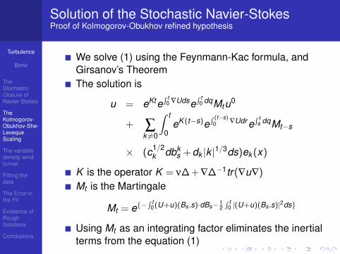
Solution of the Stochastic Navier-StokesProof of Kolmogorov-Obukhov refined hypothesis

We solve (1) using the Feynmann-Kac formula, andGirsanov’s TheoremThe solution is

u = eKte∫ t

0 ∇Udse∫ t

0 dqMtu0

+ ∑k 6=0

∫ t

0eK (t−s)e

∫ (t−s)0 ∇Udr e

∫ ts dqMt−s

× (c1/2k dbk

s + dk |k |1/3ds)ek (x)

K is the operator K = ν∆ + ∇∆−1tr(∇u∇)

Mt is the Martingale

Mt = e−∫ t

0(U+u)(Bs ,s)·dBs− 12∫ t

0 |(U+u)(Bs ,s)|2ds

Using Mt as an integrating factor eliminates the inertialterms from the equation (1)

Turbulence

Birnir




Fitting thedata

The Error inthe Fit


Conclusions

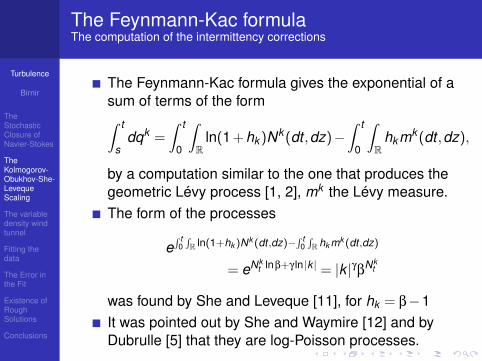
The Feynmann-Kac formulaThe computation of the intermittency corrections

The Feynmann-Kac formula gives the exponential of asum of terms of the form∫ t

sdqk =

∫ t

0

∫R

ln(1 + hk )Nk (dt ,dz)−∫ t

0

∫R

hkmk (dt ,dz),

by a computation similar to the one that produces thegeometric Lévy process [1, 2], mk the Lévy measure.The form of the processes

e∫ t

0∫R ln(1+hk )Nk (dt ,dz)−

∫ t0∫R hk mk (dt ,dz)

= eNkt lnβ+γ ln |k | = |k |γβNk

t

was found by She and Leveque [11], for hk = β−1It was pointed out by She and Waymire [12] and byDubrulle [5] that they are log-Poisson processes.

Turbulence

Birnir




Fitting thedata

The Error inthe Fit


Conclusions

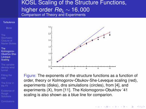
KOSL Scaling of the Structure Functions,higher order Reλ ∼ 16,000Comparison of Theory and Experiments

Figure: The exponents of the structure functions as a function oforder, theory or Kolmogorov-Obukov-She-Leveque scaling (red),experiments (disks), dns simulations (circles), from [4], andexperiments (X), from [11]. The Kolomogorov-Obukhov ’41scaling is also shown as a blue line for comparion.

Turbulence

Birnir




Fitting thedata

The Error inthe Fit


Conclusions

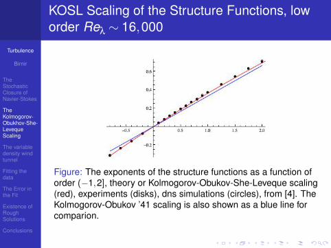
KOSL Scaling of the Structure Functions, loworder Reλ ∼ 16,000

Figure: The exponents of the structure functions as a function oforder (−1,2], theory or Kolmogorov-Obukov-She-Leveque scaling(red), experiments (disks), dns simulations (circles), from [4]. TheKolmogorov-Obukov ’41 scaling is also shown as a blue line forcomparion.

Turbulence

Birnir




Fitting thedata

The Error inthe Fit


Conclusions

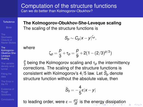
Computation of the structure functionsCan we do better than Kolmogorov-Obukhov?

The Kolmogorov-Obukhov-She-Leveque scalingThe scaling of the structure functions is

Sp ∼ Cp|x −y |ζp ,

whereζp =

p3

+ τp =p9

+ 2(1− (2/3)p/3)

p3 being the Kolmogorov scaling and τp the intermittencycorrections. The scaling of the structure functions isconsistent with Kolmogorov’s 4/5 law. Let Sp denotestructure function without the absolute value, then

S3 =−45

ε|x −y |

to leading order, were ε = dEdt is the energy dissipation

Turbulence

Birnir




Fitting thedata

The Error inthe Fit


Conclusions

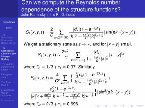
Can we compute the Reynolds numberdependence of the structure functions?John Kaminsky in his Ph.D. thesis

S1(x ,y , t) =2C ∑

k∈Z3\0

|dk |(1−e−λk t )

|k |ζ1 + 4π2ν

C |k |ζ1+

43|sin(πk · (x −y))|.

We get a stationary state as t → ∞, and for |x −y | small,

S1(x ,y , t)∼ 2πζ1

C ∑k∈Z3\0

|dk |1 + 4π2ν

C |k |43|x−y |ζ1 .

where ζ1 = 1/3 + τ1 ≈ 0.37. Similarly,

S2(x ,y , t) =4

C2 ∑k ∈Z3

C2 ck (1−e−2λk t )

|k |ζ2 + 4π2ν

C |k |ζ2+

43

+

d2k (1−e−λk t )

|k |ζ2 + 8π2ν

C |k |ζ2+

43 + 16π4ν2

C2 |k |ζ2+83

|sin2(πk · (x −y))|,

where ζ2 = 2/3 + τ2 ≈ 0.696.

Turbulence

Birnir




Fitting thedata

The Error inthe Fit


Conclusions

Higher order structure functionsThe third and pth structure functions are:

S3(x ,y , t) =8

C3 ∑k∈Z3

[ C2 ck |dk |(1−e−2λk t )(1−e−λk t )

|k |ζ3 + 8π2ν

C |k |ζ3+

43 + 16π4ν2

C2 |k |ζ3+83

+

|dk |3(1−e−λk t )3

|k |ζ3 + 12π2ν

C |k |ζ3+43 + 48π4ν2

C2 |k |ζ3+83 + 64π6ν3

C3 |k |ζ3+4

]×|sin3(πk · (x−y))|.

Sp(x ,y , t) =2p

Cp ∑k 6=0

Ap×|sinp[πk · (x −y)]|,

Ap =2

p2 Γ(p+1

2 )σpk 1F1(−1

2p, 12 ,−

12(Mk

σk)2)

|k |ζp + pk π2ν

C |k |ζp+43 + O(ν2)

,

and Mk = |dk |(1−e−λk t ), and σk =√

(C2 ck (1−e−2λk t )).

Turbulence

Birnir




Fitting thedata

The Error inthe Fit


Conclusions

Outline




4 Fitting the data



7 Conclusions

Turbulence

Birnir




Fitting thedata

The Error inthe Fit


Conclusions

The wind tunnel generating homogeneousturbulenceComparison of the new theory and experiments

The data comes from the Max Planck Institute forDynamical and Self-Orgranization, in Göttingen,Germany (E. Bodenschatz). It was generated by thevariable density turbulence tunnel (VDTT).The pressurized gases circulate in the VDTT in anupright, closed loop. At the upstream end of two testsections, the free stream is disturbed mechanically.The data in the current paper is generated by a fixedgrid, but the gas stream can also be disturbed by anactive grid resulting in even higher Reynolds numberturbulence.In the wake of the grid the resulting turbulence evolvesdown the length of the tunnel without the middle regionbeing substantially influenced by the walls of the tunnel.

Turbulence

Birnir




Fitting thedata

The Error inthe Fit


Conclusions

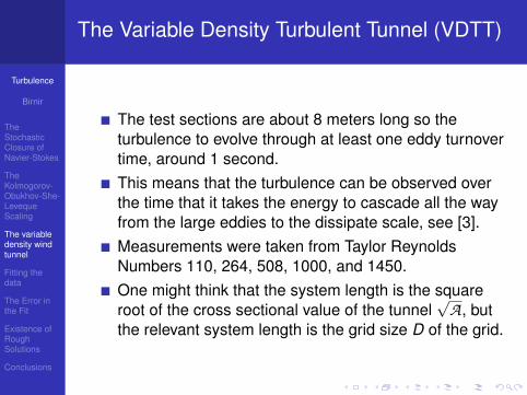
The Variable Density Turbulent Tunnel (VDTT)

The test sections are about 8 meters long so theturbulence to evolve through at least one eddy turnovertime, around 1 second.This means that the turbulence can be observed overthe time that it takes the energy to cascade all the wayfrom the large eddies to the dissipate scale, see [3].Measurements were taken from Taylor ReynoldsNumbers 110, 264, 508, 1000, and 1450.One might think that the system length is the squareroot of the cross sectional value of the tunnel

√A , but

the relevant system length is the grid size D of the grid.

Turbulence

Birnir




Fitting thedata

The Error inthe Fit


Conclusions

Outline




4 Fitting the data



7 Conclusions

Turbulence

Birnir




Fitting thedata

The Error inthe Fit


Conclusions

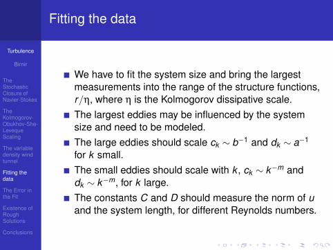
Fitting the data

We have to fit the system size and bring the largestmeasurements into the range of the structure functions,r/η, where η is the Kolmogorov dissipative scale.The largest eddies may be influenced by the systemsize and need to be modeled.The large eddies should scale ck ∼ b−1 and dk ∼ a−1

for k small.The small eddies should scale with k , ck ∼ k−m anddk ∼ k−m, for k large.The constants C and D should measure the norm of uand the system length, for different Reynolds numbers.

Turbulence

Birnir




Fitting thedata

The Error inthe Fit


Conclusions

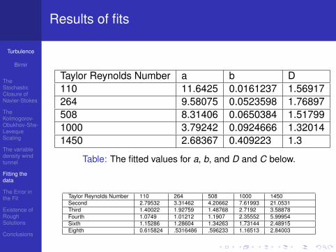
Results of fits

Taylor Reynolds Number a b D110 11.6425 0.0161237 1.56917264 9.58075 0.0523598 1.76897508 8.31406 0.0650384 1.517991000 3.79242 0.0924666 1.320141450 2.68367 0.409223 1.3

Table: The fitted values for a, b, and D and C below.

Taylor Reynolds Number 110 264 508 1000 1450Second 2.79532 3.31462 4.20662 7.61993 21.0531Third 1.40022 1.92759 1.48768 2.7192 3.58878Fourth 1.0749 1.01212 1.1907 2.35552 5.99954Sixth 1.15286 1.28604 1.34263 1.73144 2.48915Eighth 0.615824 .5316486 .596233 1.16513 2.84003

Turbulence

Birnir




Fitting thedata

The Error inthe Fit


Conclusions

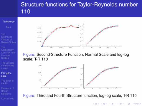
Structure functions for Taylor-Reynolds number110

Figure: Second Structure Function, Normal Scale and log-logscale, T-R 110

Figure: Third and Fourth Structure function, log-log scale, T-R 110

Turbulence

Birnir




Fitting thedata

The Error inthe Fit


Conclusions

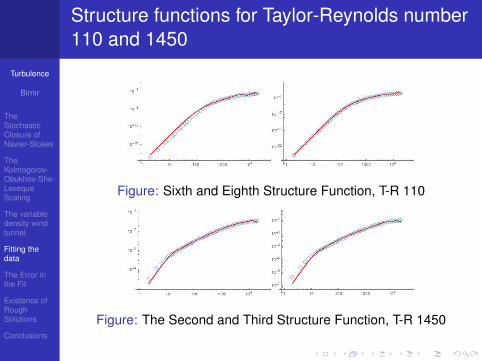
Structure functions for Taylor-Reynolds number110 and 1450

Figure: Sixth and Eighth Structure Function, T-R 110

Figure: The Second and Third Structure Function, T-R 1450

Turbulence

Birnir




Fitting thedata

The Error inthe Fit


Conclusions

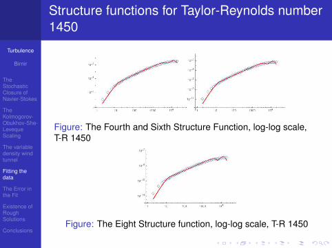
Structure functions for Taylor-Reynolds number1450

Figure: The Fourth and Sixth Structure Function, log-log scale,T-R 1450

Figure: The Eight Structure function, log-log scale, T-R 1450

Turbulence

Birnir




Fitting thedata

The Error inthe Fit


Conclusions

Onsager’s Observation

The velocity u, lies in Sobolev space Hs, where s = 116

when intermittency is not taken into account and s = 2918

when it is.This, in turn, implies that ∇u lies in Sobolev space Hs,where s = 5

6 without intermittency and s = 1118 with

intermittency, now Hs ⊂ Lp.This follows, by the Sobolev inequality, provided that

|∇u|p ≤ C‖∇u‖s,

or56≥ 3

2− 3

p.

This is true for p = 2, p = 3, and p = 4, but does nothold for p = 6 and p = 8.

Turbulence

Birnir




Fitting thedata

The Error inthe Fit


Conclusions

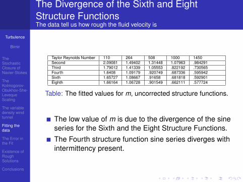
The Divergence of the Sixth and EightStructure FunctionsThe data tell us how rough the fluid velocity is

Taylor Reynolds Number 110 264 508 1000 1450Second 2.09081 1.49402 1.31448 1.07963 .984291Third 1.79012 1.41339 1.05553 .822192 .730565Fourth 1.6408 1.09179 .920749 .687336 .595942Sixth 1.65727 1.08667 .91658 .681818 .592901Eighth 1.66164 1.06728 .901549 .662111 .577724

Table: The fitted values for m, uncorrected structure functions.

The low value of m is due to the divergence of the sineseries for the Sixth and the Eight Structure Functions.The Fourth structure function sine series diverges withintermittency present.

Turbulence

Birnir




Fitting thedata

The Error inthe Fit


Conclusions

Outline




4 Fitting the data



7 Conclusions

Turbulence

Birnir




Fitting thedata

The Error inthe Fit


Conclusions

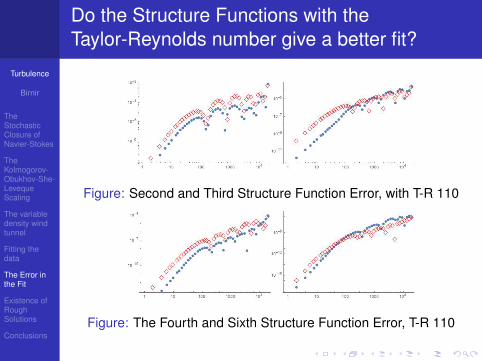
Do the Structure Functions with theTaylor-Reynolds number give a better fit?

Figure: Second and Third Structure Function Error, with T-R 110

Figure: The Fourth and Sixth Structure Function Error, T-R 110

Turbulence

Birnir




Fitting thedata

The Error inthe Fit


Conclusions

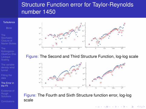
Structure Function error for Taylor-Reynoldsnumber 1450

Figure: The Second and Third Structure Function, log-log scale

Figure: The Fourth and Sixth Structure function error, log-logscale

Turbulence

Birnir




Fitting thedata

The Error inthe Fit


Conclusions

Outline




4 Fitting the data



7 Conclusions

Turbulence

Birnir




Fitting thedata

The Error inthe Fit


Conclusions

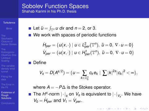
Sobolev Function SpacesShahab Karimi in his Ph.D. thesis

Let u =∫Tn u dx and n = 2, or 3.

We work with spaces of periodic functions

Hper = u(x , ·) | u ∈ L2per (Tn), u = 0, ∇ ·u = 0

Vper = u(x , ·) | u ∈ H1per (Tn), u = 0, ∇ ·u = 0

Define

Vs = D(As/2) = u = ∑k∈Zn

0

ckek | ∑ |k |2s|ck |2 < ∞,

where A =−P∆ is the Stokes operator.The Hs-norm | · |s on Vs is equivalent to | · |Vs

. We haveV0 = Hper and V1 = Vper .

Turbulence

Birnir




Fitting thedata

The Error inthe Fit


Conclusions

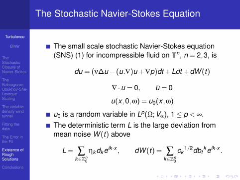
The Stochastic Navier-Stokes Equation

The small scale stochastic Navier-Stokes equation(SNS) (1) for incompressible fluid on Tn, n = 2,3, is

du = (ν∆u− (u.∇)u + ∇p)dt + Ldt + dW (t)

∇ ·u = 0, u = 0

u(x ,0,ω) = u0(x ,ω)

u0 is a random variable in Lp(Ω;Vα), 1≤ p < ∞.The deterministic term L is the large deviation frommean noise W (t) above

L = ∑k∈Zn

0

ηkdkeik ·x , dW (t) = ∑k∈Zn

0

ck1/2dbt

keik ·x .

Turbulence

Birnir




Fitting thedata

The Error inthe Fit


Conclusions

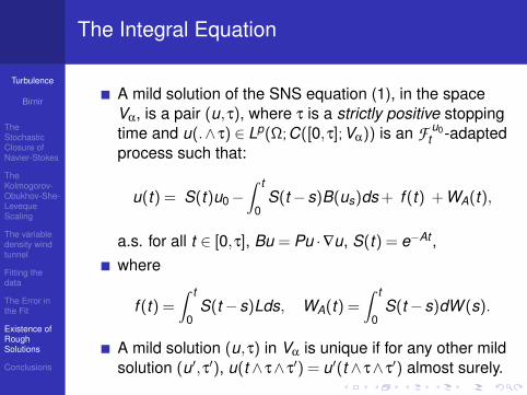
The Integral Equation

A mild solution of the SNS equation (1), in the spaceVα, is a pair (u,τ), where τ is a strictly positive stoppingtime and u(.∧ τ) ∈ Lp(Ω;C([0,τ];Vα)) is an F u0

t -adaptedprocess such that:

u(t) = S(t)u0−∫ t

0S(t−s)B(us)ds + f (t) + WA(t),

a.s. for all t ∈ [0,τ], Bu = Pu ·∇u, S(t) = e−At ,where

f (t) =∫ t

0S(t−s)Lds, WA(t) =

∫ t

0S(t−s)dW (s).

A mild solution (u,τ) in Vα is unique if for any other mildsolution (u′,τ′), u(t ∧ τ∧ τ′) = u′(t ∧ τ∧ τ′) almost surely.

Turbulence

Birnir




Fitting thedata

The Error inthe Fit


Conclusions

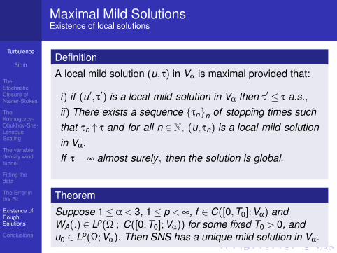
Maximal Mild SolutionsExistence of local solutions

Definition

A local mild solution (u,τ) in Vα is maximal provided that:

i) if (u′,τ′) is a local mild solution in Vα then τ′ ≤ τ a.s.,

ii) There exists a sequence τnn of stopping times suchthat τn ↑ τ and for all n ∈ N, (u,τn) is a local mild solutionin Vα.

If τ = ∞ almost surely , then the solution is global.

Theorem

Suppose 1≤ α < 3, 1≤ p < ∞, f ∈ C([0,T0];Vα) andWA(.) ∈ Lp(Ω ; C([0,T0];Vα)) for some fixed T0 > 0, andu0 ∈ Lp(Ω;Vα). Then SNS has a unique mild solution in Vα.

Turbulence

Birnir




Fitting thedata

The Error inthe Fit


Conclusions

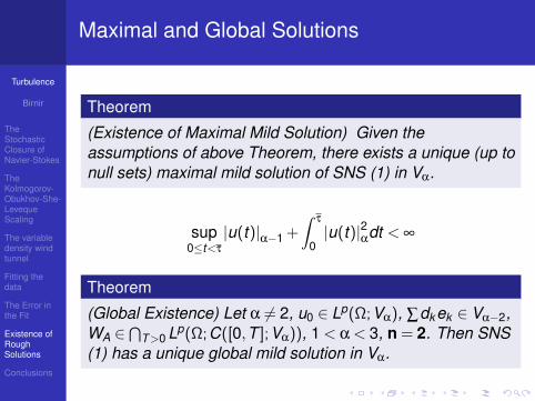
Maximal and Global Solutions

Theorem

(Existence of Maximal Mild Solution) Given theassumptions of above Theorem, there exists a unique (up tonull sets) maximal mild solution of SNS (1) in Vα.

sup0≤t<τ

|u(t)|α−1 +

∫τ

0|u(t)|2

αdt < ∞

Theorem

(Global Existence) Let α 6= 2, u0 ∈ Lp(Ω;Vα), ∑dkek ∈ Vα−2,WA ∈

⋂T>0 Lp(Ω;C([0,T ];Vα)), 1 < α < 3, n = 2. Then SNS

(1) has a unique global mild solution in Vα.

Turbulence

Birnir




Fitting thedata

The Error inthe Fit


Conclusions

Outline




4 Fitting the data



7 Conclusions

Turbulence

Birnir




Fitting thedata

The Error inthe Fit


Conclusions

Conclusions

The stochastic closure theory for Navier-Stokesreproduces the statistical theory of K-O with theintermittency corrections of She-Leveque.We computed the dependence of the structurefunctions of turbulence on the Taylor-Reynolds number.Comparisons with data from the VDTT tunnel areexcellent. The classical Prandtl windtunnel experimentis finally explained. After 100 years!Very surprisingly the data also determines thesmoothness of the fluid velocity u.Error analysis favors the Taylor-Reynolds numbercorrections and confirms the roughness of solutions:α = 4/3 and α = 2, n = 2, α = 29/18, n = 3.Existence of unique global (rough) solutions in Vα isproven, n = 2, and unique local (rough) solutions, n = 3.

Turbulence

Birnir




Fitting thedata

The Error inthe Fit


Conclusions

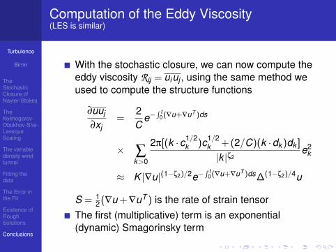
Computation of the Eddy Viscosity(LES is similar)

With the stochastic closure, we can now compute theeddy viscosity Rij = uiuj , using the same method weused to compute the structure functions

∂uuj

∂xj=

2C

e−∫ t

0(∇u+∇uT )ds

× ∑k>0

2π[(k ·c1/2k )c1/2

k + (2/C)(k ·dk )dk ]

|k |ζ2e2

k

≈ K |∇u|(1−ζ2)/2e−∫ t

0(∇u+∇uT )ds∆(1−ζ2)/4u

S = 12(∇u + ∇uT ) is the rate of strain tensor

The first (multiplicative) term is an exponential(dynamic) Smagorinsky term

Turbulence

Birnir




Fitting thedata

The Error inthe Fit


Conclusions

B. Birnir.The Kolmogorov-Obukhov statistical theory ofturbulence.J. Nonlinear Sci., 2013.DOI 10.1007/s00332-012-9164-z.

B. Birnir.The Kolmogorov-Obukhov Theory of Turbulence.Springer, New York, 2013.DOI 10.1007/978-1-4614-6262-0.

Eberhard Bodenschatz, Gregory P Bewley, HolgerNobach, Michael Sinhuber, and Haitao Xu.Variable density turbulence tunnel facility.Review of Scientific Instruments, 85(9):093908, 2014.

S. Y. Chen, B. Dhruva, S. Kurien, K. R. Sreenivasan,and M. A. Taylor.

Turbulence

Birnir




Fitting thedata

The Error inthe Fit


Conclusions

Anomalous scaling of low-order structure functions ofturbulent velocity.Journ. of Fluid Mech., 533:183–192, 2005.

B. Dubrulle.Intermittency in fully developed turbulence: inlog-poisson statistics and generalized scale covariance.Phys. Rev. Letters, 73(7):959–962, 1994.

A. N. Kolmogorov.Dissipation of energy under locally istotropic turbulence.

Dokl. Akad. Nauk SSSR, 32:16–18, 1941.

A. N. Kolmogorov.The local structure of turbulence in incompressibleviscous fluid for very large reynolds number.Dokl. Akad. Nauk SSSR, 30:9–13, 1941.

Turbulence

Birnir




Fitting thedata

The Error inthe Fit


Conclusions

A. N. Kolmogorov.A refinement of previous hypotheses concerning thelocal structure of turbulence in a viscous incompressiblefluid at high reynolds number.J. Fluid Mech., 13:82–85, 1962.

A. M. Obukhov.On the distribution of energy in the spectrum ofturbulent flow.Dokl. Akad. Nauk SSSR, 32:19, 1941.

A. M. Obukhov.Some specific features of atmospheric turbulence.J. Fluid Mech., 13:77–81, 1962.

Z-S She and E. Leveque.Universal scaling laws in fully developed turbulence.Phys. Rev. Letters, 72(3):336–339, 1994.

Turbulence

Birnir




Fitting thedata

The Error inthe Fit


Conclusions

Z-S She and E. Waymire.Quantized energy cascade and log-poisson statistics infully developed turbulence.Phys. Rev. Letters, 74(2):262–265, 1995.

Documents

Rough solutions of the Stochastic Navier-Stokes Equation · Rough solutions of the Stochastic Navier-Stokes Equation Björn Birnir Center for Complex and Nonlinear Science Department