1

Routing and charging locations for electric vehicles for intercity trips

Hong Zhenga*

and Srinivas Peetab

a. NEXTRANS Center, Purdue University, 3000 Kent Avenue, West Lafayette, IN 47906, USA b School of Civil Engineering, Purdue University, 550 Stadium Mall Drive, West Lafayette, IN 47907, USA

* Corresponding author. Email: hong112@gmail.com.

1

This study addresses two problems in the context of battery electric vehicles (EVs) for intercity trips: the EV routing

and the EV optimal charging station location problems. The paper first shows that the EV routing on the shortest

path subject to range feasibility for one origin-destination (O-D) pair, called the shortest walk problem, as well as a

stronger version of the problem – the -stop limited shortest walk problem, can be reduced to solving the shortest

path problem on an auxiliary network. Second, the paper addresses optimal charging station location problems in

which EVs are range feasible with and without stops. We formulate the models as mixed integer multi-commodity

flow problems on the same auxiliary network without path and relay pattern enumeration. The Benders

decomposition is used to propose an exact solution approach. Numerical experiments are conducted using the

Indiana state network.

Keywords: electric vehicles, routing, charging station locations, Benders decomposition

1. Introduction

Electric vehicles (EVs) have received much attention in the past few years with the promise of achieving reduced

fossil fuel dependency, enhanced energy efficiency, and improved environmental sustainability. While EVs can

achieve significantly lower operating costs and are more energy efficient (US Department of Energy, 2014a; Weaver,

2014), they have not yet been widely accepted by the traveling public. A primary reason is range anxiety which

denotes the driver concerns that the vehicle will run out of battery power before reaching the destination. This is a

serious issue, particularly for long or intercity trips (Mock et al., 2010; Yu et al., 2011).

Given the current battery technologies, an EV typically has a range of around 100 miles with a full charge,

depending on the motor type, vehicle size and battery pack style (US Department of Energy, 2014b). For example,

the 2015 Nissan Leaf and Chevrolet Spark EVs have a driving range of about 80 miles. The Tesla (model X and S)

EV with its advanced battery technology has a higher range of around 250-350 miles which is expected to improve

further (Tesla Motors, 2014). The charging time depends on the electric power connector, charging schemes, and

battery capacity (Botsford and Szczepanek, 2009). It usually takes 6-10 hours for an EV to be fully charged in a

slow charging mode (level I and II, see Table 1). For example, it takes the Nissan Leaf equipped with an 80kW

motor 8 hours to recharge for a 240V 3.6 kW on-board charger, and 5.5 hours for a 240V 6.6 kW charger (level II).

The Tesla Model S equipped with a 225kW motor with 60kWh battery pack takes about 10 hours for a 240V single

charger (US Department of Energy, 2014b). Fast charging technology, which requires a level III power connector,

can enable a range of over 100 miles with as little as a ten-minute charging time. It supplies direct current of up to

550A, 600V and specifies power level of the charger up to 500kW (Botsford and Szczepanek, 2009). Currently, the

fast charging operation is much more costly than level II charging, and thus these facilities are sparsely deployed in

the public domain. While fast charging can reduce the charging time, range anxiety concerns cannot be eliminated in

the near future due to the fast charging’s inability to provide a full charge in a limited amount of time. This is

because batteries currently require longer time to charge fully the closer they are to full charge, and hence fast

charging typically focuses on obtaining about 80% charge in a certain time duration.

Table 1. Charging schemes for electric vehicles

Types of charge Level I Level II Level III

Power (kW) 1.4 6.6 14.4

Charging voltage 120V, 15A 120V and 240V, 30A Up to 600V, 550A

Another technology that has been investigated to address the EV range limitation is battery exchange/swapping

(Senart et al., 2010). At battery exchange/swapping stations, a pallet of depleted batteries is removed from an EV

and replaced with a fully recharged battery (Squatriglia, 2009). Battery exchange can be performed quickly, usually

in minutes, but requires identical pallets and batteries. Battery exchange has been practiced in Israel, and is an

available option in Denmark (Environmental Defense Fund, 2014). Recently, Tesla Motors announced plans to open

battery swapping stations in California (Edelstein, 2014).

The range limitation specifies the maximum distance an EV can travel without stopping to recharge. The actual

range of an EV is relevant to several factors including travel speed, terrain, battery state of charge, temperature, etc.

2

In this paper, the travel range is assumed to be a fixed quantity corresponding to the normally encountered traffic

conditions in the rural context of typical intercity trips. The range limitation is an issue not only for EVs, but also for

vehicles that use alternative fuels as they need to find alternative fuel refueling facilities to successfully complete the

trip (Kang and Recker, 2012; Kuby and Lim, 2005, 2007; Ogden et al., 1999; Wang and Lin, 2009). Hence,

alternative fuel vehicles are also subject to a range limitation, and similar to EVs, need to visit the appropriate

refueling stations to complete a long or intercity trip.

This paper addresses two problems in the context of EVs for intercity trips. First, it analyzes the EV routing

problem subject to the range limitation. EVs are assigned on the shortest path in an auxiliary network, where each

arc represents a range feasible walk in the original network. The problem is similar to the EV range-constrained

shortest walk problem (Adler et al., 2014; Mirchandani et al., 2014) analyzed for a single origin-destination (O-D)

pair, but extended to the case of one origin to multiple destinations. It is shown that the EV shortest walk problem

from one origin to multiple destinations, as well as the -stop limited shortest walk problem (where an EV stops to

recharge at most times) from one origin to multiple destinations, have the same complexity as the corresponding

single O-D pair cases. This enables computational efficiency for planners, who seek EV routing feasibility for

multiple O-D pairs. Further, we show that the -stop limited shortest walk problem can be solved efficiently using a

dynamic programming, which is simpler than the existing method of creating an expanded network with multiple

layers. Note that , the number of stops, is a parameter herein rather than a decision variable. The associated EV

shortest walk problem minimizing is NP-complete (Ichimori et al., 1983). The -stop limited problem is a

restricted problem. Because en route charging can involve a significant amount of charging time (fast or slow

charging), EVs aim to recharge as few times as possible to reduce the en route charging time. Thereby, the -stop

limited problem can be viewed as the EV drivers not accepting routes with more than stops.

The unrestricted EV routing problem subject to range feasibility is a simplified version of bi-criteria weight

constraint shortest path problem (Beasley and Christofides, 1989). In it, there are two arc attributes, arc cost and

weight. The goal is to find the least cost path subject to a limit on the accumulation of weight. Similar to the EV

range limitation context, replenishment can be set on either nodes or arcs to reset the accumulated weight to zero;

the corresponding problems are known as the shortest path problem with relays (Laporte and Pascoal, 2011), or the

shortest path problem with replenishment arcs (Smith et al., 2012). In Laporte and Pascoal (2011), nodes can be

used as relays to reset the transported weight to zero. They present both a label-setting and a label-correcting

algorithm for the problem where all costs and weights are assumed to be non-negative and integer. In Smith et al.

(2012), replenishment occurs at arcs. They present a label-correcting method incorporating replenishment, and

explore several different label structure and treatment strategies. Further, they use a high-level network, called meta-

network, to exploit the inter-replenishment sub-path structure of feasible paths (Smith et al., 2012). Such solutions

consist of sequences of weight-feasible paths between replenishment arcs. Their meta-network is similar to the

auxiliary network in which we solve the EV routing problem. The methods discussed heretofore (Laporte and

Pascoal, 2011, Smith et al. 2012) can solve the general weight constraint shortest path problem, including the

unrestricted EV routing problem, efficiently. However, the routing problem in this study has specific characteristics

associated with EVs. For example, an EV usually does not accept a route that has more than stops, and thus we

consider the -stop limited problem in the EV context, which is a significant difference from the shortest path

problem with relays (Laporte and Pascoal, 2011) or with replenishment arcs (Smith et al., 2012).

Second, the paper addresses the optimal charging station location problems (CSLPs) subject to range feasibility

with and without stops. The unrestricted problem without stops is known as the network design problem with

relays (NDPR) (Cabral et al., 2007, Konak, 2012) in the operations research literature. The NDPR locates relays at a

subset of nodes in the graph such that there exists a path linking the origin and the destination for each commodity

for which the length between the origin and the first relay, the last relay and the destination, or any two consecutive

relays does not exceed a preset upper bound. The NDPR arises in telecommunications and logistic systems where

the payload must be reprocessed at intermediate stations called relays (Cabral et al., 2007). Although conceptually

similar to NDPR, a key difference exhibited by our CSLP is that the charging facilities (or relay nodes) in our study

consider capacity. In the real-world, because an EV will consume time to charge its battery, the maximum number

3

of EVs that can be served at a charging facility within a certain period is subject to an upper bound due to service

time. This feature makes the EV CSLP a capacitated network design problem while the NDPR is an uncapacitated

one. Further, EVs may travel on multiple paths in the CSLP whereas in the NDPR each commodity is routed on a

single path which simplifies the problem. The -stop limited CSLP is even more complex than the NDPR due to the

-stop constraint.

Cabral et al. (2007) studied the NDPR in the context of telecommunication network design. They formulated

the problem as a path-based integer programming model and proposed a column generation method for solving the

problem. This column generation method is not practical because it requires the enumeration of all possible paths

and relay locations a priori. Because each combination of possible path and relay pattern is represented as a binary

variable, the model formulation entails a huge number of binary variables. Cabral et al. used column generation to

solve a linear programming (LP) relaxation of the problem to generate the column set, and then solved the integer

problem with the generated column set. This approach may not generate an optimal solution because the generated

column set is restricted and does not guarantee the inclusion of the optimal column set. In the numerical experiments

reported in Cabral et al. (2007), the optimality gaps are more than 100% in most instances. Konak (2012) proposed a

set covering formulation with a meta-heuristic algorithm for the NDPR. It still enumerates the path set for each

commodity, which precludes the efficient design of an exact solution algorithm.

In this study, we propose a different network flow based model formulation. Specifically, the EV CSLPs are

formulated as multi-commodity mixed integer linear programs on the same auxiliary network developed for the EV

routing problem. Solution algorithms based on Benders decomposition are proposed to determine the exact solution

in a real-sized problem with small optimality gap. Due to their conceptual similarity in the problem context,

“charging”, “refueling” and “relays” are viewed interchangeably in this study. Hence, the methodologies

investigated here for EV charging also apply to the NDPR and alternative fuel vehicle refueling context.

The study contributions are as follows. First, it is shown that the -stop EV routing can be solved using

dynamic programming through one shortest-path computation on an auxiliary network, which is conceptually

simpler than the method of Adler et al. (2014) that creates a multi-level expanded network containing copies

of the nodes. Second, most prior studies investigate EV routing/equilibria without considering the determination of

the optimal charging station locations, and assume them to be pre-determined inputs. By contrast, this study

investigates the CSLPs under range feasibility. The CSLP is different from NDPR due to limited capacity at

charging facilities and -stop constraint in EV routing. Third, unlike the existing NDPR studies, this study proposes

a different network flow based mixed integer model formulation. As any feasible path on the established auxiliary

network respects the range limitation constraint, our link-based formulation (rather than a path-based formulation)

avoids enumerating the path set and the relay pattern set. A solution algorithm based on Benders decomposition is

designed to determine the exact solution with small optimality gap.

The remainder of the paper is organized as follows. Section 2 reviews relevant literature on the EV routing and

charging/refueling location problems. Section 3 addresses the EV routing problem. Section 4 addresses the charging

station location problem. Numerical experiments are analyzed in Section 5. Section 6 provides some concluding

comments.

2. Literature review of EV studies

Past studies relevant to EVs in the transportation domain can be broadly grouped into three categories: EV energy-

efficient routing, EV equilibrium assignment, and EV facility location of charging stations. Sachenbacher et al.

(2011) introduced the problem of determining the most energy-efficient path for EVs with recuperation in a graph-

theoretical context. Here, a recuperation capability implies that EVs can be equipped with regenerative braking

systems to recuperate a part of the kinetic energy lost during the deceleration phase so as to recharge the battery.

Artmeier et al. (2010) and Storandt (2012) proposed revised shortest-path algorithms to address the energy-optimal

routing. They formulated energy-efficient routing in the presence of rechargeable batteries as a special case of the

constrained shortest path problem and presented an adaptation of a shortest path algorithm. Ichimori et al. (1983)

and Adler et al. (2014) studied the EV shortest walk problem to determine the route from an origin to a destination

4

with minimum detouring; this route may include cycles for detouring to recharge batteries. Ichimori et al. (1983)

further showed that the EV shortest walk problem minimizing the number of stops is polynomial-time reducible to

the vertex cover problem, and is hence NP-complete. In a dynamic context, Schneider et al. (2014) investigated the

EV routing problem with custom time windows. Conrad and Figliozzi (2011) introduced the charging vehicle

routing problem, wherein vehicles with limited range must service a predetermined set of customers and may

recharge at specific customer locations in order to continue a tour. It can be used for EVs with fast charging

capabilities carrying short distance less-than-truckload deliveries in urban areas. The problem is an extension of the

distance-constrained vehicle routing problem (Figliozzi, 2008; Li et al., 1992).

Network equilibrium models have been studied for the EV class in the literature. Considering EV with no

charging capability, Jiang et al. (2012) formulated a multi-class path constrained traffic assignment model for mixed

EVs and internal combustion engine (ICE) vehicles. In it, the EV is one vehicle class with trip length no more than

the range of full battery capacity, and thus EVs’ equilibrium routes are restricted to the set of distance-constrained

paths. Jiang and Xie (2014) extended their model to the combined mode choice and assignment framework. In this

model, the EV class still has no capability to recharge, and travelers select vehicle class and route jointly. This

implies that travelers own both EV and ICE vehicles. Their analysis suggests that for the set of routes with length

less than the range, all travelers select EVs; and, for the set of routes with length beyond the range, all travelers

select ICE vehicles. Traffic equilibrium is then achieved for the two path sets. He et al. (2014) addressed single class

network equilibrium by considering EVs with charging capabilities. Their objective is to minimize the traditional

user equilibrium term plus the charging time. Most studies discussed heretofore consider network equilibrium with

flow-independent energy consumption, that is, EV travel cost is only related to the distance traveled and

independent of the traffic congestion. He et al. (2014) consider flow-dependent energy consumption to model EV

equilibria as a variational inequality (VI). In general, the aforementioned EV equilibrium models do not consider the

optimal deployment of the charging station locations.

Several studies have investigated the facility location problem of charging stations (Baouche et al., 2014; Chen

et al., 2013; He et al., 2013; Sellmair and Hamacher, 2014; Xi et al., 2013) and battery swapping stations (Mak et al.,

2013). Nie and Ghamami (2013) addressed the selection of the battery size and charging capacity to meet a given

level of service such that the total social cost is minimized. Mirchandani et al. (2014) addressed several logistic

issues of EVs with battery swap, which include EV routing, charging location, and scheduling problem for electric

buses. They showed that planned scheduling of EV fleet of buses to the routes and charging stations can reduce the

amount of energy used by the buses. The corresponding EV fleet scheduling problem, however, is NP-hard.

Mirchandani et al. also investigated the problem of locating minimum number of swapping stations such that the

total detouring cost for a single O-D pair flow is minimized. He et al. (2013) investigated the charging station

location problem for plug-in hybrid electric vehicles (PHEVs), wherein there is no range constraint for PHEVs.

They assumed that PHEVs are always charged at trip destinations. So, travelers are assumed to jointly select routes

and destinations based upon charging prices at destinations.

Alternative fuel refueling models mainly focus on the refueling station location problem. Hodgson (1990)

developed the first flow-capturing location model (FCLM), a flow-based maximal covering problem locates

facilities to maximize the flow volume captured. In FCLM, a flow is captured if at least one facility is located

anywhere along the path of flow without considering the driving range limitation. To enhance FCLM, Kuby and

Lim (Kuby and Lim, 2007; Lim and Kuby, 2010) studied the flow-refueling location model (FRLM) that is designed

to locate refueling stations so as to refuel the maximum volume of traffic flows traveling on their shortest paths

subject to the range limitation. Upchurch et al. (2009) extended the model to account for the limited capacity of the

refueling stations. A similar refueling location problem was investigated by Wang and Lin (2009) using the concept

of set covering. Wang (2007, 2008) explored the battery swapping location model to optimally meet the needs of

electric scooters used by tourists. In a nutshell, in the aforementioned alternative fuel refueling location studies,

vehicles travel on the shortest path for each O-D pair without restriction on the maximum number of stops/refuels.

Further, the model formulations are path-based. In our study, however, the charging location problem considers the

maximum number of stops/recharges, and proposes different model formulations and solution algorithms.

5

3. Electric vehicle routing

This section discusses the EV routing problem. The EV routing is subject to the range constraint imposed by the

battery technology. The battery range of an EV trip is denoted by , which represents the maximum length an EV

can travel without charging. Here, “charging” is used to broadly represent battery recharge, battery exchange, or any

other options to obtain a fully charged battery for the EV to continue its intercity travel.

Let denote a directed graph, where denotes a set of nodes and a set of arcs. Let and

. Let denote an origin and a destination. EVs are assigned from to in . A walk is represented by a

set of nodes visited in sequence, i.e., . If each node in is visited only once, the walk is also

labeled a path. Each arc in is associated with a distance (or length) , where . The length of a path (or

walk) is the summation of lengths of arcs contained in the path (or walk). Denote by a set of charging

stations whose geographic locations are known.

A walk is range feasible if the following condition holds: a sub-walk between any two

successive nodes in contained in has a length at most . For example, consider a walk

and the charging location . Then, two pairs of successive nodes in are and

. The range feasibility implies that both sub-walk and sub-walk are no longer than . The

EV routing problem assigns the EV on a walk from to such that the walk is range feasible and the length is the

shortest. This EV routing problem was studied by Adler et al. (2014), where the problem is referred to as the EV

shortest walk problem (EV-SWP). They show that EV-SWP is polynomially solvable. A stronger version of the

problem, EV-SWP subject to stops (charging stations are visited at most times) is also polynomially solvable. In

this paper, we extend the EV-SWP and the -stop EV-SWP for a single O-D pair in Adler et al. (2014) to the case of

multiple destinations. The proposed method leverages the fact that both EV-SWP and -stop EV-SWP can be

reduced to solving the shortest path problem (SPP) on an auxiliary network, as discussed hereafter.

Problem 1: Electric vehicle shortest walk problem (EV-SWP) (Adler et al., 2014)

Find a shortest walk in starting at and ending at such that the walk is range feasible. □

The EV-SWP can be polynomially reduced to a general shortest path problem on an auxiliary graph. Build a

complete graph between the set of nodes as follows. For any pair of nodes ,

compute the shortest length from to in , denoted by . If , we create an arc such that the

cost of the arc, denoted by , equals the shortest length . Therefore, each arc represents a shortest

path from to in . Building requires solving the all-to-all shortest path problem with nodes, and thus

the complexity is (for example, Floyd-Warshall algorithm). The EV-SWP then becomes the problem

of finding the shortest path from to in . The rationale of the problem reduction is that if there is a walk from

node to node and , then such a walk must follow one shortest path from to in .

Proposition 1: The EV-SWP can be solved in .

Proof. Building the auxiliary graph requires time to solve the all-to-all shortest path problem

using the Floyd-Warshall algorithm. contains at most nodes and arcs. Therefore,

solving the shortest path problem in requires .

The overall complexity of solving EW-SWP is .□

This complexity is slightly worse than in Adler et al. (2014). However, the approach

illustrated heretofore can be trivially extended to the case with multiple destinations.

Problem 2: Electric vehicle shortest walk problem for multiple destinations (EV-SWP-M)

Given an origin and a set of destinations , find a walk from to each destination such that any

walk from to is the shortest and range feasible. □

6

The case of multiple destinations is a little different from the single O-D pair case. We build an auxiliary graph

as follows. For any pair of nodes and , , compute the shortest length from to in

, denoted by . If , we create an arc such that the cost of the arc equals . Different from

the case of the single O-D pair, the set of destination nodes cannot be visited as intermediate nodes in the path

found in ; otherwise, it may violate the range feasibility. Therefore, in there are no outbound arcs

originating from , which restricts that a node in cannot be visited by a path found in unless it is the

destination. This, however, does not restrict visiting the set of nodes in in the shortest walk in graph , because

each arc represents a shortest path from to in which may visit nodes in in .

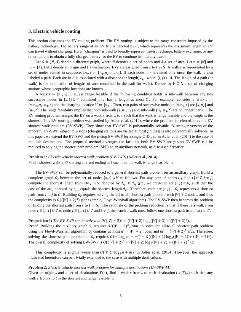
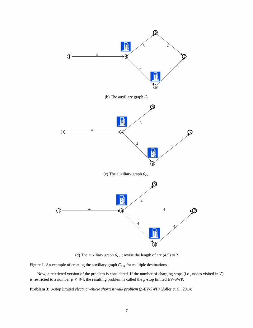
Figure 1 illustrates an example of creating for multiple destinations, and its difference from the single O-D

pair case. Suppose the driving range is 5. Applying the rule used to create for the single O-D pair, that is, for any

pair of nodes , create an arc if the shortest length from to in (shown in Figure

1(a)) is no more than . The auxiliary graph shown in Figure 1(b) is created, where the shortest path from 1 to 7 is

{1,4,5,7}. Here, the sub-walk {4,5,7} has a length 7, which is more than the range 5, violating the range limitation.

Figure 1(c) illustrates the rule of creating the auxiliary graph ; there are no outbound arcs associated with

destinations 5 and 7, hence the shortest path from 1 to 7 is {1,4,6,7}, which maintains range feasibility. To

demonstrate that the destination node 5 could be visited as an intermediate node in the shortest walk in , revise the

length of arc (4,5) to 2. Then the auxiliary graph is as shown in Figure 1(d), where the shortest path from 1 to 7

is {1,4,7}, which represents the shortest walk {1,2,4,5,7} in . It can be observed that the destination node 5 is

visited by the shortest walk in although it is not visited in the auxiliary graph because the arc (4,7) in

represents the shortest walk {4,5,7} in .

The EV-SWP-M is equivalent to solving a shortest path tree in . As solving the shortest path has the same

effort as solving the shortest path tree, EV-SWP and EV-SWP-M have the same complexity.

Proposition 2: The EV-SWP-M can be solved in

( + +1)2), where | | represents number of destinations.

Proof. Same as Proposition 1. □

1

3

4

2

6

5

7

2

3 3

3

2

4

5

2

44

1 is origin, 5 and 7 are destinations, 4 and 6 are charging locations, range is 5

(a) Network

7

1 4

6

5

7

5 2

4 4

4

(b) The auxiliary graph

1 4

6

5

7

5

44

4

(c) The auxiliary graph

1 4

6

5

7

2

4

4 4

4

(d) The auxiliary graph ; revise the length of arc (4,5) to 2

Figure 1. An example of creating the auxiliary graph for multiple destinations.

Now, a restricted version of the problem is considered. If the number of charging stops (i.e., nodes visited in )

is restricted to a number , the resulting problem is called the -stop limited EV-SWP.

Problem 3: -stop limited electric vehicle shortest walk problem (p-EV-SWP) (Adler et al., 2014)

8

Finding a shortest walk in starting at and ending at such that the walk is range feasible and charging occurs at

most times. □

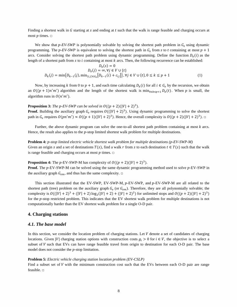
We show that -EV-SWP is polynomially solvable by solving the shortest path problem in using dynamic

programming. The -EV-SWP is equivalent to solving the shortest path in from to containing at most

arcs. Consider solving the shortest path problem using dynamic programming. Define the function as the

length of a shortest path from to containing at most arcs. Then, the following recurrence can be established:

(1)

Now, by increasing from 0 to , and each time calculating for all by the recursion, we obtain

an algorithm and the length of the shortest walk is . When is small, the

algorithm runs in .

Proposition 3: The -EV-SWP can be solved in .

Proof. Building the auxiliary graph requires . Using dynamic programming to solve the shortest

path in requires . Hence, the overall complexity is . □

Further, the above dynamic program can solve the one-to-all shortest path problem containing at most arcs.

Hence, the result also applies to the -stop limited shortest walk problem for multiple destinations.

Problem 4: -stop limited electric vehicle shortest walk problem for multiple destinations (p-EV-SWP-M)

Given an origin and a set of destinations , find a walk from to each destination such that the walk

is range feasible and charging occurs at most times. □

Proposition 4: The -EV-SWP-M has complexity of .

Proof. The -EV-SWP-M can be solved using the same dynamic programming method used to solve -EV-SWP in

the auxiliary graph , and thus has the same complexity. □

This section illustrated that the EV-SWP, EV-SWP-M, -EV-SWP, and -EV-SWP-M are all related to the

shortest path (tree) problem on the auxiliary graph (or ). Therefore, they are all polynomially solvable; the

complexity is for unlimited stops and

for the -stop restricted problem. This indicates that the EV shortest walk problem for multiple destinations is not

computationally harder than the EV shortest walk problem for a single O-D pair.

4. Charging stations

4.1. The base model

In this section, we consider the location problem of charging stations. Let denote a set of candidates of charging

locations. Given charging station options with construction costs for , the objective is to select a

subset of such that EVs can have range feasible travel from origin to destination for each O-D pair. The base

model does not consider the -stop limitation.

Problem 5: Electric vehicle charging station location problem (EV-CSLP)

Find a subset set of with the minimum construction cost such that the EVs between each O-D pair are range

feasible. □

9

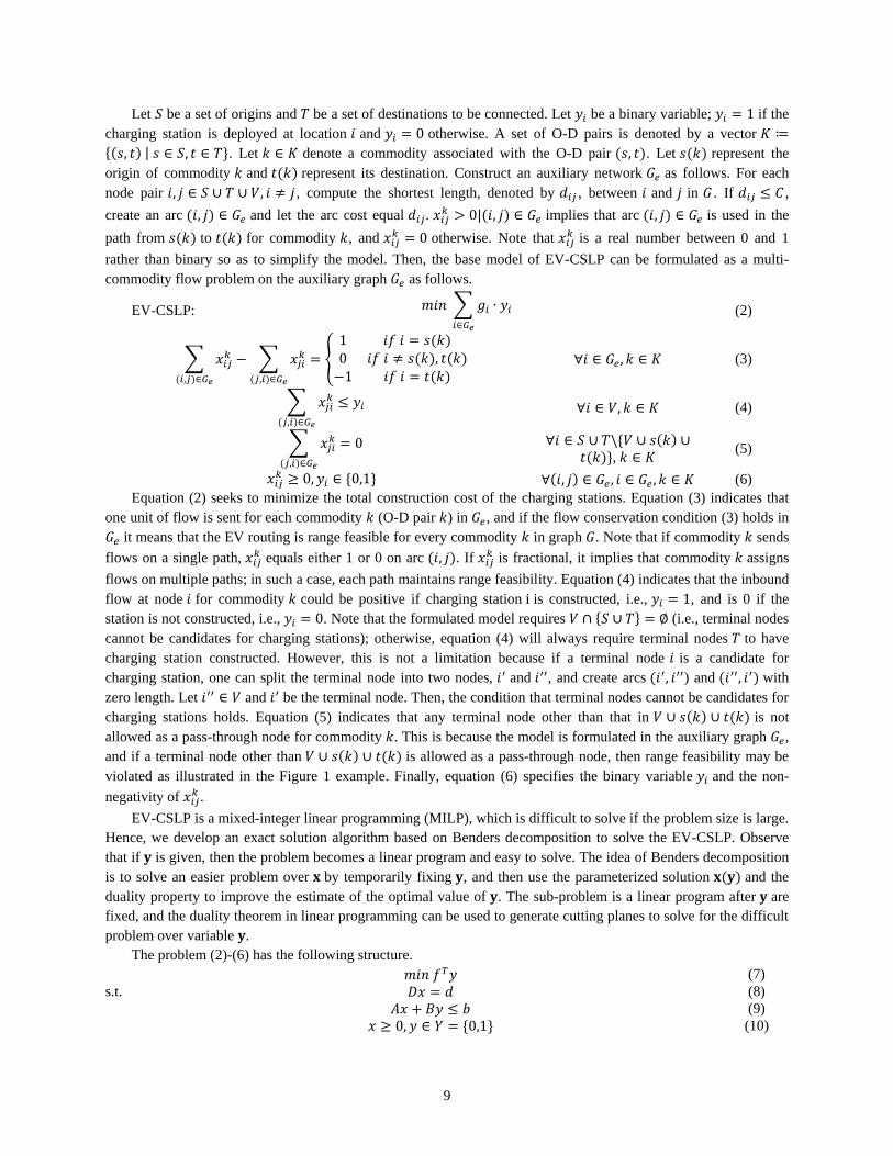
Let be a set of origins and be a set of destinations to be connected. Let be a binary variable; if the

charging station is deployed at location and otherwise. A set of O-D pairs is denoted by a vector

. Let denote a commodity associated with the O-D pair . Let represent the

origin of commodity and represent its destination. Construct an auxiliary network as follows. For each

node pair , compute the shortest length, denoted by , between and in . If ,

create an arc and let the arc cost equal . implies that arc is used in the

path from to for commodity , and otherwise. Note that

is a real number between 0 and 1

rather than binary so as to simplify the model. Then, the base model of EV-CSLP can be formulated as a multi-

commodity flow problem on the auxiliary graph as follows.

EV-CSLP:

(2)

(3)

(4)

,

(5)

(6)

Equation (2) seeks to minimize the total construction cost of the charging stations. Equation (3) indicates that

one unit of flow is sent for each commodity (O-D pair ) in , and if the flow conservation condition (3) holds in

it means that the EV routing is range feasible for every commodity in graph . Note that if commodity sends

flows on a single path, equals either 1 or 0 on arc . If

is fractional, it implies that commodity assigns

flows on multiple paths; in such a case, each path maintains range feasibility. Equation (4) indicates that the inbound

flow at node for commodity could be positive if charging station is constructed, i.e., , and is 0 if the

station is not constructed, i.e., . Note that the formulated model requires (i.e., terminal nodes

cannot be candidates for charging stations); otherwise, equation (4) will always require terminal nodes to have

charging station constructed. However, this is not a limitation because if a terminal node is a candidate for

charging station, one can split the terminal node into two nodes, and , and create arcs ) and with

zero length. Let and be the terminal node. Then, the condition that terminal nodes cannot be candidates for

charging stations holds. Equation (5) indicates that any terminal node other than that in is not

allowed as a pass-through node for commodity . This is because the model is formulated in the auxiliary graph ,

and if a terminal node other than is allowed as a pass-through node, then range feasibility may be

violated as illustrated in the Figure 1 example. Finally, equation (6) specifies the binary variable and the non-

negativity of .

EV-CSLP is a mixed-integer linear programming (MILP), which is difficult to solve if the problem size is large.

Hence, we develop an exact solution algorithm based on Benders decomposition to solve the EV-CSLP. Observe

that if is given, then the problem becomes a linear program and easy to solve. The idea of Benders decomposition

is to solve an easier problem over by temporarily fixing , and then use the parameterized solution and the

duality property to improve the estimate of the optimal value of . The sub-problem is a linear program after are

fixed, and the duality theorem in linear programming can be used to generate cutting planes to solve for the difficult

problem over variable .

The problem (2)-(6) has the following structure.

(7)

s.t. (8)

(9)

(10)

10

Benders decomposition partitions the problem (7)-(10) into two problems: (i) a master problem that contains the

variables, and (ii) a sub-problem that contains the variables. The master problem is as follows.

(11)

s.t. (12)

where is defined to be the optimal objective function value of:

(13)

s.t. (14)

(15)

(16)

Formulation (13)-(16) is a linear program for any given value of . The objective function (13) indicates

that the problem needs to solve for a feasible solution and does not have a specific objective. Instead of solving

directly, Benders decomposition solves by solving its dual. This is based on the key observation that the

feasible region of the dual formulation does not depend on the value of , which only affects the objective function.

Let us associate dual variable (unrestricted) with Eq. (14) and with Eq. (15). Then the dual problem is:

(17)

s.t. (18)

unrestricted, (19)

Let variable , matrix

, and vector

; then the dual problem has the following

structure.

(20)

s.t. (21)

Assuming that the feasible region of (20)-(21) is not empty, we can enumerate all extreme points

and extreme directions

, where and are the number of extreme points and extreme directions,

respectively. Using the extreme points and extreme directions, the dual problem can be reformulated as the

following equivalent problem.

(22)

s.t. (23)

(24)

Now, the dual-sub problem has the form (22)-(24), and the original master problem (11)-(12) becomes the

following formulation depending on the and varaibles.

(25)

s.t. (26)

(27)

unrestricted (28)

Since there is exponential number of extreme points and extreme directions, enumerating all constraints of type

(26) and (27) are not practical. Instead, Benders decomposition starts with a subset of these constraints, and solves a

“relaxed master problem”, which obtains a candidate optimal solution . It then solves the dual sub-problem

(20)-(21) to calculate . If the dual-sub problem has an optimal solution with , then the algorithm

stops with an optimal solution. If the dual-sub problem is unbounded, then a constraint of the type (26), labeled the

Benders feasibility cut, is generated and added to the relaxed master problem. If the dual-sub problem has an

optimal solution with , then a constraint of the type (27), labeled the Benders optimality cut, is generated

and added to the relaxed master problem. The relaxed master problem is then resolved with the added cut. Since

and are finite, new feasibility and optimality cuts are generated in each iteration, and the method converges to an

optimal solution in a finite number of iterations.

11

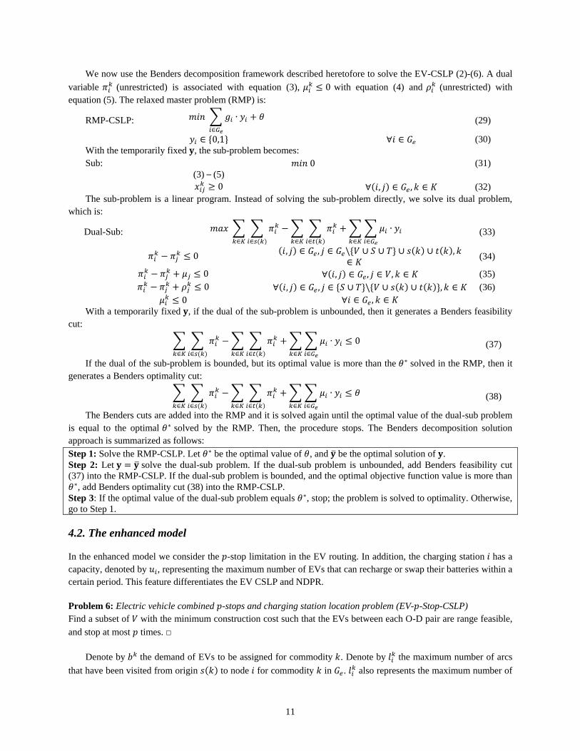
We now use the Benders decomposition framework described heretofore to solve the EV-CSLP (2)-(6). A dual

variable (unrestricted) is associated with equation (3),

with equation (4) and (unrestricted) with

equation (5). The relaxed master problem (RMP) is:

RMP-CSLP:

(29)

(30)

With the temporarily fixed , the sub-problem becomes:

Sub: (31)

(3) – (5)

(32)

The sub-problem is a linear program. Instead of solving the sub-problem directly, we solve its dual problem,

which is:

Dual-Sub:

(33)

(34)

(35)

(36)

With a temporarily fixed , if the dual of the sub-problem is unbounded, then it generates a Benders feasibility

cut:

(37)

If the dual of the sub-problem is bounded, but its optimal value is more than the solved in the RMP, then it

generates a Benders optimality cut:

(38)

The Benders cuts are added into the RMP and it is solved again until the optimal value of the dual-sub problem

is equal to the optimal solved by the RMP. Then, the procedure stops. The Benders decomposition solution

approach is summarized as follows:

Step 1: Solve the RMP-CSLP. Let be the optimal value of , and be the optimal solution of .

Step 2: Let solve the dual-sub problem. If the dual-sub problem is unbounded, add Benders feasibility cut

(37) into the RMP-CSLP. If the dual-sub problem is bounded, and the optimal objective function value is more than

, add Benders optimality cut (38) into the RMP-CSLP.

Step 3: If the optimal value of the dual-sub problem equals , stop; the problem is solved to optimality. Otherwise,

go to Step 1.

4.2. The enhanced model

In the enhanced model we consider the -stop limitation in the EV routing. In addition, the charging station has a

capacity, denoted by , representing the maximum number of EVs that can recharge or swap their batteries within a

certain period. This feature differentiates the EV CSLP and NDPR.

Problem 6: Electric vehicle combined -stops and charging station location problem (EV- -Stop-CSLP)

Find a subset of with the minimum construction cost such that the EVs between each O-D pair are range feasible,

and stop at most times. □

Denote by the demand of EVs to be assigned for commodity . Denote by the maximum number of arcs

that have been visited from origin to node for commodity in . also represents the maximum number of

12

charging stations that have been visited by the EVs. Denote an auxiliary variable which is 1 if arc is used by

commodity , and 0 otherwise. The EV- -Stop-CSLP can be formulated in the following link-based formulation.

EV- -Stop-CSLP:

(39)

(40)

(41)

,

(42)

(43)

(44)

(45)

(46)

(47)

(48)

Equation (39) seeks to minimize the construction cost. Equation (40) assigns demand along paths in . Note

that due to the limited capacity at charging stations, maybe assigned on multiple paths. The flow conservation

condition being satisfied in implies that flow is feasible subject to the range limitation for each utilized path.

Equation (41) indicates that flow can be positive if the charging location is constructed, and the total

commodity flow visiting charging location is no larger than its capacity ; must be zero if the charging

location is not constructed. Similar to the base model, equation (42) indicates that any node other than

cannot represent a pass-through node for commodity in . Equation (43) specifies that if is positive, arc

is utilized for commodity , and hence . Otherwise,

, which indicates is not utilized for

commodity , and thereby .

is an auxiliary variable. Equation (44) indicates that the inbound arcs for

node can be utilized only if the charging facility is constructed at . Equation (44) links variables and .

Equation (45) specifies that if , then

increases by one. If , then equation (45) becomes redundant.

implies the maximum number of charging stations visited from to for commodity . Equation (46)

indicates that the maximum number of visited charging locations is bounded by at each node for each commodity.

Equation (47) specifies the initial condition of which equals zero at the origin node for each commodity .

Equation (48) specifies the binary variables and , and the non-negativity of

and .

The solution algorithm again applies the Benders decomposition. We associate a dual variable (unrestricted)

with equation (40), and

with equations (41)-(43), (45)-(47),

respectively. The relaxed master problem (RMP) is:

RMP- -CSLP:

(49)

(44)

, (50)

With the temporarily fixed and , the sub-problem becomes:

-Sub: (51)

(40)-(43),(45)-(47)

(52)

The -sub problem is a linear program. For Benders decomposition, we solve the dual problem of -sub as

follows.

13

Dual- -

Sub:

(53)

s.t.

(54)

(55)

, (56)

(57)

(58)

(59)

(60)

(61)

With a temporarily fixed and e, if the dual of the sub-problem is unbounded, then it generates a Benders

feasibility cut:

(62)

If the dual of the sub-problem is bounded, but its optimal value is more than the solved in the RMP, then it

generates a Benders optimality cut:

(63)

The Benders cuts are added into the RMP and it is solved again until the optimal value of the dual-sub is equal

to the optimal solved by the RMP. Then, the procedure stops. The Benders decomposition solution approach can

be stated as follows:

Step 1: Solve the RMP- -CSLP. Let be the optimal value of , and , be the optimal solutions of and e,

respectively.

Step 2: Let , solve the dual- -sub problem. If the dual- -sub problem is unbounded, add Benders

feasibility cut (62) into the RMP- -CSLP. If the dual- -sub problem is bounded, and the optimal objective function

value is more than , add Benders optimality cut (63) into the RMP- -CSLP.

Step 3: If the optimal value of dual- -sub equals , stop; the problem is solved to optimality. Otherwise, go to Step

1.

5. Numerical examples

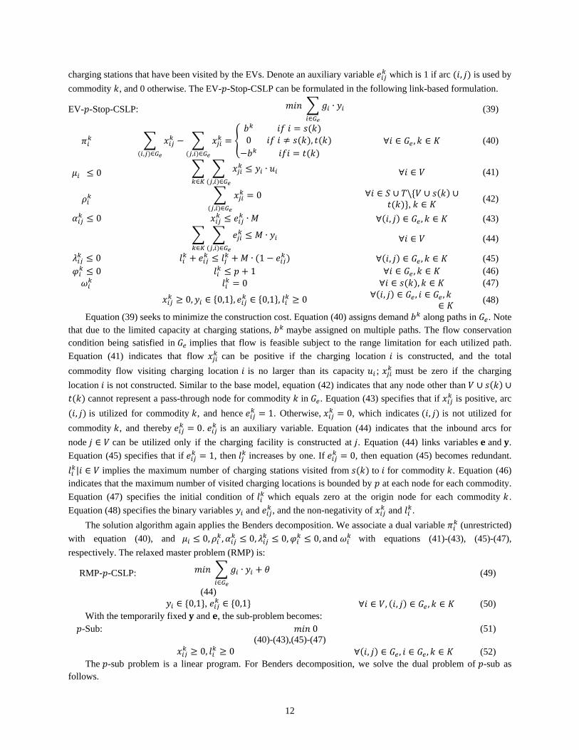
5.1. An illustrative hypothetical network example

We consider the small hypothetical network shown in Figure 2. is the origin and is the destination. Suppose the

battery range is 8, and the charging stations . The auxiliary graph is built in Figure 3. It can be

14

verified that the shortest walk from to is the shortest path in , i.e., , which has a length 12. This path

exhibits the shortest walk in , that is, . It can be verified that both sub-walks and

satisfy the range limitation, and thus the walk is range feasible.

There are two 1-stop-limited walks in the network, i.e., and in , or and

in . Among them, the latter is the walk with the shortest distance. It is range infeasible to travel

from to without stops; so, the minimum number of stops is 1. Note that both paths in have two arcs in their

paths. While the walk visits two charging stations, i.e., 5 and 11, the EV does not need to recharge at

11 because the distance from 5 to is 6 which is less than the feasible range. Hence, the walk is a 1-

stop-limited walk as exhibited in .

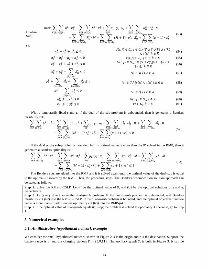
Next, we solve the charging location problem in this example. Suppose nodes 1 to 13 are candidates for

charging stations, and their construction costs are as shown in Table 2. Five destinations are considered in this

problem, . We solve the minimum charging location problem such that each O-D pair is range

feasible and has 2-limited stops. The auxiliary graph is built in Figure 4.

Table 2. Cost of charging stations in the illustrative hypothetical network example. Charging station Cost Charging station Cost

1 100 8 110

2 50 9 70

3 80 10 80

4 30 11 60

5 200 12 120

6 150 13 90

7 50

s

1

2

3

4

5

6

7

8

9

11

12

13

10

t

xdistance

2

Figure 2. Example hypothetical network.

15

s 8 5

9

11

t

xdistance

Figure 3. The auxiliary graph for EVs routing with charging locations .

s

1

2

3

4

5

6

7

8

9

11

12

13

10

t

xdistance

8

5

3

Figure 4. The auxiliary graph with candidates for charging locations 1-13.

16

s

1

2

3

4

5

6

7

8

9

11

12

13

10

t

xdistance

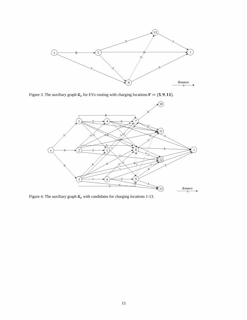
2

Shortest walk

Figure 5. Charging locations and 2-stop limited shortest walks in the network.

5.2. A real-world network example

The Indiana state network, shown in Figure 6, is used as a real-world network to illustrate the proposed methods.

The network consists of 17 cities with populations of more than 50,000, and 25 links. These cities are connected by

I-65 and U.S. highways, as shown in the figure. There are 9 traffic analysis zones (TAZs) and 81 O-D pairs. The

network is of medium size in the current practice of EV planning. As the EV demand in future years is not available,

the O-D trips in this study are hypothetical as shown in Table 3, and the total number of trips is 16,400. All cities are

candidates for charging locations. The capacities of the charging stations are assumed to be commensurate with the

population and the cost. The capacity and cost data are shown in

Table 4. The full battery range is assumed to be 150 miles, consistent with the optimal range forecasted in a recent

study (Lin, 2014). The auxiliary graph has 34 nodes and 368 arcs; hence, the -stop CSLP involves 368 81 =

29,808 binary variables of , and 17 binary variables of . Therefore the total number of binary variables is 29,825.

The size of the formulated mixed-integer linear program is very large and the problem is difficult to solve. The

Benders decomposition approach discussed in Section 4 is used to determine the optimal charging station locations

with the minimum construction cost, under the assumption that each O-D pair is range feasible and EVs stop at most

2 times. The problem is solved using CPLEX 12.1 interfaced with Python 2.7 on a personal computer equipped with

a 2.66-GHz Intel(R) Xeon(R) E5640 CPU with 24 GB of memory.

Table 3. O-D demand data. Origins\Destinations Indianapolis Fort Wayne Evansville South Bend Bloomington Gary Lafayette Terre Haute Louisville

Indianapolis 0 500 400 300 300 250 250 200 400

Fort Wayne 500 0 200 200 200 200 200 200 200

Evansville 400 200 0 200 200 200 200 200 200

South Bend 300 200 200 0 200 200 200 200 200

Bloomington 300 200 200 200 0 200 200 200 200

Gary 250 200 200 200 200 0 200 200 200

Lafayette 250 200 200 200 200 200 0 200 200

Terre Haute 200 200 200 200 200 200 200 0 200

Louisville 400 200 200 200 200 200 200 200 0

17

Table 4. Cost and capacities of charging stations in the real-world example. City Cost ($) Capacity (number of vehicles)

Indianapolis 500,000 5,000

Fort Wayne 250,000 2,500

Evansville 250,000 2,500

South Bend 250,000 2,500

Bloomington 250,000 5,000

Gary 250,000 2,500

Lafayette 250,000 2,500

Terre Haute 250,000 2,500

Louisville 250,000 2,500

Kokomo 100,000 1,000

Anderson 100,000 1,000

Noblesville 100,000 1,000

Elkhart 100,000 1,000

Muncie 100,000 1,000

Fishers 100,000 1,000

Carmel 100,000 1,000

Hammond 100,000 1,000

Figure 6. The Indiana state network.

18

Indianapolis

Fort Wayne

Evansville

South Bend

Carmel

Bloomington

Fishers

Hammond Gary

Muncie

Lafayette

Terre Haute

Kokomo

Anderson

Noblesville

Elkhart

Louisville

36

Figure 7. Travel distance of Indiana state network.

When the capacity constraint is not considered, the results of the optimal charging locations in this case are

Kokomo and Bloomington, as indicated in Figure 8(a). Only two charging stations are required to ensure the range

feasibility. The total construction cost is $350,000. It can be verified that between each O-D pair EVs are range

feasible, and stop to recharge at most twice.

When the capacity constraint is considered, Benders decomposition is applied to solve the -stop problem

where . The computational time to solve the problem to optimality is 74 minutes. The optimal charging

locations are Kokomo, Fishers, Lafayette and Bloomington. Because of the limited capacity in Kokomo, two more

charging stations are needed. Fishers and Lafayette are selected because of the low construction costs. Each O-D

pair is range feasible and EVs recharge at most twice. The total construction cost is $1.1 million. In this case,

Indianapolis is not selected because while it can provide enough capacity, its construction cost (which includes the

land cost) is expensive. Also, Fishers is a suburb of Indianapolis. The results suggest that instead of constructing

large charging stations with enough capacity in a single city, it is desirable to deploy the charging stations so that

they geographically spread with limited capacities, due to the range feasibility limitation and potential facility costs.

19

Indianapolis

Fort Wayne

Evansville

South Bend

Carmel

Bloomington

Fishers

Hammond Gary

Muncie

Lafayette

Terre Haute

Kokomo

Anderson

Noblesville

Elkhart

Louisville

36

Indianapolis

Fort Wayne

Evansville

South Bend

Carmel

Bloomington

Fishers

Hammond Gary

Muncie

Lafayette

Terre Haute

Kokomo

Anderson

Noblesville

Elkhart

Louisville

36

(a) Optimal charging locations without capacity

constraint

(b) Optimal charging locations with capacity constraint

Figure 8. Optimal charging location station deployment in the Indiana state network.

6. Conclusions

In this paper, we investigate the EV routing and optimal deployment of charging locations subject to the range

limitation. The EV routing subject to the range feasibility for the case of a single origin to multiple destinations is

shown to have the same complexity as that of a single O-D pair. A stronger version of the problem, the -stop

problem for the case of single origin to multiple destinations is not harder than the case of the single O-D pair, either.

Specifically, the four routing problems, EV shortest walk problem for a single O-D pair, EV shortest walk for a

single origin, -stop shortest walk problem for a single O-D pair, and -stop shortest walk problem for a single

origin, are all solvable by the shortest path algorithm on an auxiliary network. The difference is that the -stop

version of the problem uses a dynamic programming method to solve for the shortest path problem on the auxiliary

network.

The problem of optimal charging locations is analyzed. Each O-D pair is subject to range feasibility and EVs

are assumed to recharge at most times. The unrestricted problem (EVs can recharge with unlimited stops) is

known as the NDPR. In this paper, the -restricted problem is modeled as a mixed-integer multi-commodity flow

problem on the auxiliary network. In contrast to the prior NDPR methodologies, we present a link-based formulation

which circumvents feasible path and relay pattern enumeration. The problem involves a significant amount of binary

variables and is hence difficult to solve. We develop a novel solution algorithm based on Benders decomposition,

20

which is designed to determine the exact solution. A numerical example on a real-world network (the Indiana state

network) is analyzed, and shows that the Benders decomposition approach can determine the exact solution in a

reasonable amount of time. Due to the conceptual similarity, the proposed methodologies apply to the network

design problem with relays.

In the Benders decomposition method, the dual sub-problem is a feasibility problem. In our model formulation

the method generates feasibility cuts which are significantly more in number than the number of optimality cuts, and

thus the convergence could be slow, particularly at the initial stage where the feasibility cuts are not tight. The role

of feasibility cuts is to guarantee that the lower bound obtained from the relaxed master problem is valid and the role

of the optimality cuts is to restrict the lower bound. Thus, producing more optimality cuts would lead to faster

convergence of the Benders decomposition method (Magnanti and Wong, 1981; Saharidis and Ierapetritou, 2010).

Exploring algorithmic strategies to accelerate Benders decomposition by producing tight cuts is a future research

direction.

The EV routing problem in this study assigns flows on the shortest path; there is no congestion effect and the

operating cost is flow-independent. In the real world, traffic involves congestion in the network and the EVs will

likely factor travel time in the selection of the shortest route. It leads to a traffic equilibrium model subject to the

range feasibility. Investigating the equilibrium model of EVs subject to the range feasibility, combined with the

optimal charging location deployment, is another future research direction.

References

Adler, J.D., Mirchandani, P.B., Xue, G., Xia, M., 2014. The electric vehicle shortest-walk problem with battery exchanges.

Networks and Spatial Economics, in press.

Artmeier, A., Haselmayr, J., Leucker, M., Sachenbacher, M., 2010. The shortest path problem revisited: optimal routing for

electric vehicles. Lecture Notes in Computer Science: 309-316.

Baouche, F., Billot, R., Trigui, R., Faouzi, N.-E.E., 2014. Efficient allocation of electric vehicles charging stations: optimization

model and application to a dense urban network. Intelligent Transportation Systems Magazine, IEEE, 6(3): 33-43.

Beasley, J.E., and Christofides, N., 1989. An algorithm for the resource constrained shortest path problem. Networks, 19(4): 379-

394.

Botsford, C., Szczepanek, A., 2009. Fast charging vs. slow charging: pros and cons for the new age of electric vehicles EVS 24,

Stavanger, Norway.

Cabral, E.A., Krkut, E., Laporte G., Patterson, R.A. 2007. The network design problem with relays. European Journal of

Operational Research, 180(2): 834-844.

Chen, T.D., Kockelman, K.M., Khan., M., 2013. The electric vehicle charging station location problem: a parking-based

assignment method. 93rd Annual Meeting of the Transportation Research Board, Washington, DC.

Edelstein, S., 2014. Tesla to introduce electric car battery swapping stations in California within months. www.ecomento.com.

Environmental Defense Fund. 2014. Automated EV battery swap for faster refuel. www.edf.org/energy/innovation/.

Figliozzi, M.A., 2008. Planning approximations to the average length of vehicle routing problems with varying customer

demands and routing constraints. Transportation Research Record: Journal of the Transportation Research Board, 2089:

1-8.

Gonrad, R.G., Figliozzi, M.A., 2011. The recharging vehicle routing problem. T. Doolen, E.V. Aken, eds. Proceedings of the

2011 Industrial Engineering Research Conference.

He, F., Wu, D., Yin, Y., Guan, Y., 2013. Optimal deployment of public charging stations for plug-in hybrid electric vehicles.

Transportation Research Part B: Methodological, 47: 87-101.

He, F., Yin, Y., Lawphongpanich, S., 2014. Network equilibrium models with battery electric vehicles. Transportation Research

Part B: Methodological, 67: 306-319.

Hodgson, M.J., 1990. A flow capturing location-allocation model. Geographical Analysis, 22(3): 270-279.

Ichimori, T., Ishii, H., Nishida, T., 1983. Two routing problems with the limitation of fuel. Discrete Applied Mathematics, 6(1):

85-89.

Jiang, N., Xie, C., 2014. Computing and analyzing mixed equilibrium network flows with gasoline and electric vehicles.

Computer-Aided Civil and Infrastructure Engineering, 29(8): 626-641.

Jiang, N., Xie, C., Waller, S.T., 2012. Path-constrained traffic assignment: model and algorithm. Transportation Research Record:

Journal of the Transportation Research Board, 2283: 25-33.

Kang, J.E., Recker, W.W., 2012. Strategic hydrogen refueling station locations with scheduling and routing considerations of

individual vehicles UCI-ITS-WP-12-2. University of California, Irvine.

Konak, A. 2012. Network design problem with relays: A genetic algorithm with a path-based crossover and a set covering

formulation. European Journal of Operational Research, 218(3): 829-837.

21

Kuby, M., Lim, S., 2005. The flow-refueling location problem for alternative-fuel vehicles. Socio-Economic Planning Sciences,

39(2): 125-145.

Kuby, M., Lim, S., 2007. Location of alternative-fuel stations using the flow-refueling location model and dispersion of candidate

sites on arcs. Networks and Spatial Economics, 7(2): 129-152.

Laporte, G. and Pascoal, M.M.B., 2011. Minimum cost path problems with relays. Computers & Operations Research, 38: 165-

173.

Li, C.-L., Simchi-Levi, D., Desrochers, M., 1992. On the distance constrained vehicle routing problem. Operations Research,

40(4): 790-799.

Lim, S., Kuby, M., 2010. Heuristic algorithms for siting alternative-fuel stations using the Flow-Refueling Location Model.

European Journal of Operational Research, 2014: 51-61.

Lin, Z., 2014. Optimizing and diversifying electric vehicle driving range for U.S. drivers. Transportation Science, in press.

Mak, H.Y., Rong, Y., Shen, Z.J.M., 2013. Infrastructure planning for electric vehicles with battery swapping. Management

Science, 59(7): 1557-1575.

Magnanti, T., Wong, R., 1981. Accelerating Benders decomposition algorithmic enhancement and model selection criteria.

Operations Research, 29(3): 464–484.

Mirchandani, P., Adler, J., Madsen, O.B.G., 2014. New logistical issues in using electric vehicle fleets with battery exchange

infrastructure. Procedia - Social and Behavior Sciences, 108: 3-14.

Mock, P., Schmid, S., Friendrich, H., 2010. Market prospects of electric passenger vehicles. G. Pistoia, ed. Electric and Hybrid

Vehicles: Power Sources, Models, Sustainability, Infrastructure and the Market. Elsevier, Amsterdam, Netherlands.

Nie, Y., Ghamami, M., 2013. A corridor-centric approach to planning electric vehicle charging infrastructure. Transportation

Research Part B: Methodological, 57: 172-190.

Ogden, J.M., Steinbugler, M.M., Kreutz, T.G., 1999. A comparison of hydrogen, methanol and gasoline as fuels for fuel cell

vehicles: implications for vehicle design and infrastructure development. Journal of Power Sources, 79(2): 143-168.

Sachenbacher, M., Leucker, M., Artmeier, A., Haselmayr, J., 2011. Efficient energy-optimal routing for electric vehicles.

Proceedings of the Twenty-Fifth AAAI Conference on Artificial Intelligence.

Saharidis, G. K., Ierapetritou, M. G., 2010. Improving Benders decomposition using maximum feasible subsystem (MFS) cut

generation strategy. Computers & Chemical Engineering, 34(8): 1237-1245.

Schneider, M., Stenger, A., D. Goeke. 2014. The electric vehicle-routing problem with time windows and recharging stations.

Transportation Science, 48(4): 500-520.

Sellmair, R., Hamacher, T., 2014. Optimization of charging infrastructure for electric taxis. Transportation Research Record:

Journal of the Transportation Research Board, 2416: 82-91.

Senart, A., Kurth, S., Roux, G.L., Antipolis, S., Street, N.C., 2010. Assessment framework of plug-in electric vehicles strategies.

Smart Grid Communications, 2010 First IEEE International Conference on: 155-160.

Squatriglia, C., 2009. Better place unveils and electric car battery swap station. http://www.wired.com/2009/05/better-place/.

Smith, O.J., Boland, N. and Waterer, H. 2012. Solving shortest path problems with a weight constraint and replenishment arcs.

Computers & Operations Research, 39: 964-984.

Storandt, S., 2012. Quick and energy-efficient routes –computing constrained shortest paths for electric vehicles. IWCTS '12

Proceedings of the 5th ACM SIGSPATIAL International Workshop on Computational Transportation Science.

Tesla Motors. 2014. www.teslamotors.com.

Upchurch, C., Kuby, M., Lim, S., 2009. A model for location of capacitated alternative-fuel stations. Geographical Analysis,

41(1): 85-106.

US Department of Energy. 2014a. http://www.afdc.energy.gov/fuels/electricity_benefits.html.

US Department of Energy. 2014b. www.fueleconomy.gov.

Wang, Y.W., 2007. An optimal location choice model for recreation-oriented scooter recharge stations. Transportation Research

Part D: Transport and Environment, 12(3): 231-237.

Wang, Y.W., 2008. Locating battery exchange stations to serve tourism transport: a note. Transportation Research Part D:

Transport and Environment, 13(3): 193-197.

Wang, Y.W., Lin, C.C., 2009. Locating road-vehicle refueling stations. Transportation Research Part E: Logistics and

Transportation Review, 45(5): 821-829.

Weaver, L., 2014. Top three reasons for choosing an electric vehicle. http://alternativefuels.about.com/od/electricvehicles/a/Top-

Three-Reasons-For-Choosing-An-Electric-Vehicle.htm.

Xi, X., Sioshansi, R., Marano, V., 2013. Simulation-optimization model for location of a public electric vehicle charging

infrastructure. Transportation Research Part D: Transport and Environment, 22: 60-69.

Yu, A.S.O., Silva, L.L.C., Chu, C.L., Nascimento, P.T.S., Camargo, A.S., 2011. Electric vehicles: struggles in creating a market.

Technology Management in the Energy Smart World: 1-13.

View publication statsView publication stats