RR2011 - The comparison of 7 HFO · PDF fileMUMM Oostende (BE) Marijke Neyts Petrobras Rio de Janeiro (BR) Fabiana D. C. Gallotta ... The accident occurred 200 miles off the coast

BONN AGREEMENT Oil Spill Identification

Network of Experts

CEDRE

Centre de documentation, de

recherché et d'expérimentations

sur les pollutions accidentelles des

eaux.

RR2011 - The comparison of 7 HFO

samples

Sixth intercalibration in the framework of Bonn-OSINET

The results of nineteen international laboratories

Date 3 March 2014

Status Final version

On the front page:

Heavy Fuel Oil on the French coast

RR2011 - The comparison of 7 HFO

samples

Sixth intercalibration in the framework of Bonn-OSINET

The results of nineteen international laboratories

Colophon

Department WGML

Information Paul Kienhuis

Telephone:

0031 6 11 876 989

E-mail: [email protected]

Authors P. Kienhuis and G. Dahlmann,

Clients RR2011 participants,

RWS-WD_Department WGML,

RWS-North Sea and

Bonnagreement

Dated: 3 March 2014

Status Final version

Document # 2012.WGMLO 41xx

RR2011 - The comparison of 7 HFO samples | 17 april 2012

Page 4 of 55


Page 5 of 55

Contents

Executive summary 7

1 Introduction 11

2 Instructions 13

3 Real scenario 17

4 Evaluation of the case following CEN/TR 15522-2v2 v51. 19 4.1 Preliminary remark 19 4.2 GC-FID 20 4.3 GC-MS 22 4.3.1 First visual inspection 22 4.3.2 Spill 1- source 1 22 4.3.3 Spill 2 – source 1 24 4.3.4 Spill 3 and spill 4 – source 1 25 4.3.5 Spill 5 and spill 6 – source 1 28

5 Common aspects of the reports 29 5.1 Sample treatment 29 5.2 Variance of the duplicate analyses of the source sample 30 5.3 Oil type recognition. 31 5.4 Normative compound/ratio exclusion 35 5.5 Informative compound integration. 35

6 Table 2 evaluation 39

7 Evaluation of the weathering of oil by IMOF. 41

8 Judgement of the individual reports. 47 8.1 Evaluation methods 47 8.2 Evaluation method of Gerhard 47 8.3 Evaluation method of Paul 48 8.4 Judgement of the results 48

9 Conclusions 51 9.1 Summarizing conclusion 53

10 References 55


Page 6 of 55


Page 7 of 55

Executive summary

Round Robin 2011 (RR2011) was the sixth world-wide ring test of the expert group

on oil spill identification of the Bonn-Agreement (Bonn-OSINET), in which 19

laboratories from 14 countries participated.

Laboratory Location Contact

EPA-CES Victoria (AU) Syed Hasnain

NSWDECC Lidcombe (AU) Steve Fuller

MUMM Oostende (BE) Marijke Neyts

Petrobras Rio de Janeiro (BR) Fabiana D. C. Gallotta

EC-ALET Moncton (CA) Josee Losier

ESTS Ottawa (CA) Chun Yang

ALS Edmonton (CA) Deib Birkholz

NCSEMC Qingdao (CN) Sun Peiyan

BSH Hamburg (DE) Gerhard Dahlmann

EERC Tallinn (EE) Krista Mötz

CSIC Barcelona (ES) Joan Albaiges

NBI Helsinki (FI) Niina Viitala

CEDRE Brest (FR) Julien Guyomarch

LASEM Toulon (FR) Francois Davids

Total Harfleur (Fr) Pierre Giusti

LVA Riga (LV) Irina Dzene

RWS-WD Lelystad (NL) Paul Kienhuis

Sintef Trondheim (NO) Liv-Guri Faksness/ Kjersti Almås

SKL Linköping (SE) Helen Turesson/Magnus Kallberg

The laboratories received seven heavy fuel oil (HFO) samples related to a large oil

spill that occurred in 2001 for the French coast. According to the proposed scenario

two of the samples were collected in the year of the spill and four of the samples

were collected 10 years after the spill.

It was requested to work (if possible) according to draft version 51 of CEN/Tr

15522-2, published in September 2011 on the BonnOSInet - OSPAR web-server. It

is the same version that has been submitted to CEN as an update for CEN/Tr 15522-

2 (2006). A technical report should be returned and two spreadsheet files, which

were provided to the participants, should be filled with the measured data. The

spreadsheet files should / could already be used to evaluate the analytical results by

means of ratio comparisons and MS-PW-plots.

The reason to select these samples is to test whether the last update of the CEN/Tr

is suitable to use for oil spill identification of very weathered oil samples.

In the real scenario spill samples 1 and 2 were prepared from artificially-weathered

oil from the source sample. Spill samples 3 and 4 were collected on a contaminated

beach. Spill sample 5 was also from a beach but on a place that was related to a

different spill. Spill 6 was prepared from an artificial weathered different HFO.

On request of several participants Paul Kienhuis and Gerhard Dahlmann judged the

reports of the participants this year for the first time. Points were given to aspects

Table 1

Participants of RR2011


Page 8 of 55

like analytical quality of the data, assessment of the case and conclusions of oil type

and match conclusions. The final judgement was calculated as a percentage of the

maximum number of points that could be achieved.

In the summary report of RR2011, that is made available in public on the Bonn

agreement website, the results of the participants are presented anonymously by

means of a code for each lab.

The match conclusions of the laboratories are presented in Table 1.

Lab code Spill 1 Spill 2 Spill 3 Spill 4 Spill 5 Spill 6

Scenario M M PM PM NM NM

Lab1 M NM I I no results no results

Lab2 M M PM/I PM/I I I

Lab3 M M NM PM I I

Lab4 M PM PM PM NM NM

Lab5 M M NM / PM NM / PM NM NM

Lab6 M PM PM PM PM PM

Lab7 M PM NM I NM NM

Lab8 M M I PM NM NM

Lab9 M M NM NM NM NM

Lab10 M M I I I I

Lab11 PM PM PM NM NM I

Lab12 PM PM I PM I I

Lab13 M NM NM NM NM NM

Lab14 PM NM NM NM NM NM

Lab15 M M PM PM NM NM

Lab16 M NM I I I I

Lab17 M M PM PM NM NM

Lab18 no results no results no results no results no results no results

Lab19 PM PM NM PM NM NM

In this Round Robin all participants had problems to evaluate the severely

weathered spill samples. Most labs have given a clear conclusion for the artificial

weathered spill samples 1, 2 and 6, but were much more unsure regard to the real

spill samples. Insufficient knowledge about the fate of oil in severely weathered oil

samples was given as a reason. Several participants indicated that in a real case

one would take much more samples and follow the process of weathering much

closer.

For a Round Robin this is however not possible.

For the judgement of the reports two methods were used. Gerhard and Paul made

both an own judgement method and evaluated the reports each with both methods.

The results of the judgement of the reports are given in Table 2.

Table 2

Match conclusions of the

labs for the spill samples in

relation with the provided

source sample:

M = match;

PM=probable match;

I = inconclusive;

NM = non-match.

Differences of “more than

one” match conclusion apart

from the true conclusion are

indicated in bold


Page 9 of 55

Lab code Method Paul Method Gerhard mean

Lab1 81 79 80

Lab2 100 100 100

Lab3 88 83 85

Lab4 100 100 100

Lab5 38 39 38

Lab6 56 52 54

Lab7 94 97 95

Lab8 100 100 100

Lab9 69 76 72

Lab10 88 82 85

Lab11 88 88 88

Lab12 75 82 78

Lab13 75 73 74

Lab14 81 74 78

Lab15 81 77 79

Lab16 81 88 85

Lab17 100 100 100

Lab18

Lab19 94 97 95

After combining the results it can be concluded that the differences between the two

methods are small.

No points were given to the contribution of Lab 18. This lab participated for the first

time and had problems with entering the analytical data into the provided

spreadsheet files. Therefore no judgement was given.

Table 3 shows that many labs were able to write a good report, but also that some

labs have problems. This is often related to the fact, that they have a very limited

number of actual cases and are therefore less skilled in oil spill identification.

With regard to the test of the CEN-method, RR2011 was a very special and

problematic case. The participants got only a very small insight in post spill

investigations, and it has to be discussed, whether information of this kind can or

should be included in a next update of the method.

Table 3

Results of the judgement of

the reports as % of the

maximum reachable

number of points.


Page 10 of 55


Page 11 of 55

1 Introduction

At the OSINET meeting in Barcelona 2011, Pierre Giusti and Julien Guyomarch gave

a short presentation about their investigations in the Erika-case, which happened at

the end of 2001, and which led to a massive oil pollution at the French coast. Even

11 years after this accident, pollution is still present at some places. Identification of

the oil is difficult because this oil is extremely heavily weathered. Pierre and Julien

stated that the CEN-guideline was used, but this method seemed not to be

appropriate here: the compounds to calculate the DRs were often so heavily

weathered that barely ratios were left for comparison.

Other ratios were mentioned, which mainly are used in geochemical investigations,

and which obviously were more stable over the long time of weathering. It was

proposed to improve the DRs of the CEN-guideline with these ratios.

To get experience with this kind of samples and to test the new ratios, it was

decided that Pierre and Julien select relevant samples and arrange a scenario for the

round robin of 2011. They have also built a spreadsheet file that contains the

intended ratios and that should be used by the participants as an additional tool for

sample comparison.


Page 12 of 55


Page 13 of 55

2 Instructions

On 14-9-11 the instructions for RR2011 were published on the Bonn-OSINET forum:

Subject: Oil Spill Identification Round Robin 2011

From: Julien Guyomarch, Ronan Jezequel, Paul Kienhuis and Gerhard Dahlmann

Dear Colleagues,

For the sixth oil spill identification intercalibration round within the Bonn-OSINET

expert group you have received 7 samples.

You may regard 7 samples as too many for an inter-calibration as normally only up to

5 samples were sent. But we want to make this RR more interesting. Two of these samples

were sent for special purposes (see below), and may be analyzed or not depending on your time

and interest. But please notice: „real“ and rare samples are included!

Scenario and samples information:

In 2001, a tanker ran into a heavy storm and broke in two and sank, releasing thousands of tons

of oil into the sea. The accident occurred 200 miles off the coast of Brittany, and thousands of

kilometres of the shoreline were impacted. Few days after the accident, a sample representative

of the cargo was received and was considered as the reference oil (source 1). In the next few

months, many samples were collected to ensure the origin of the oil when cleaning beaches and

rocks covered with oil. Ten years later, several samples were collected for analyses. Reference

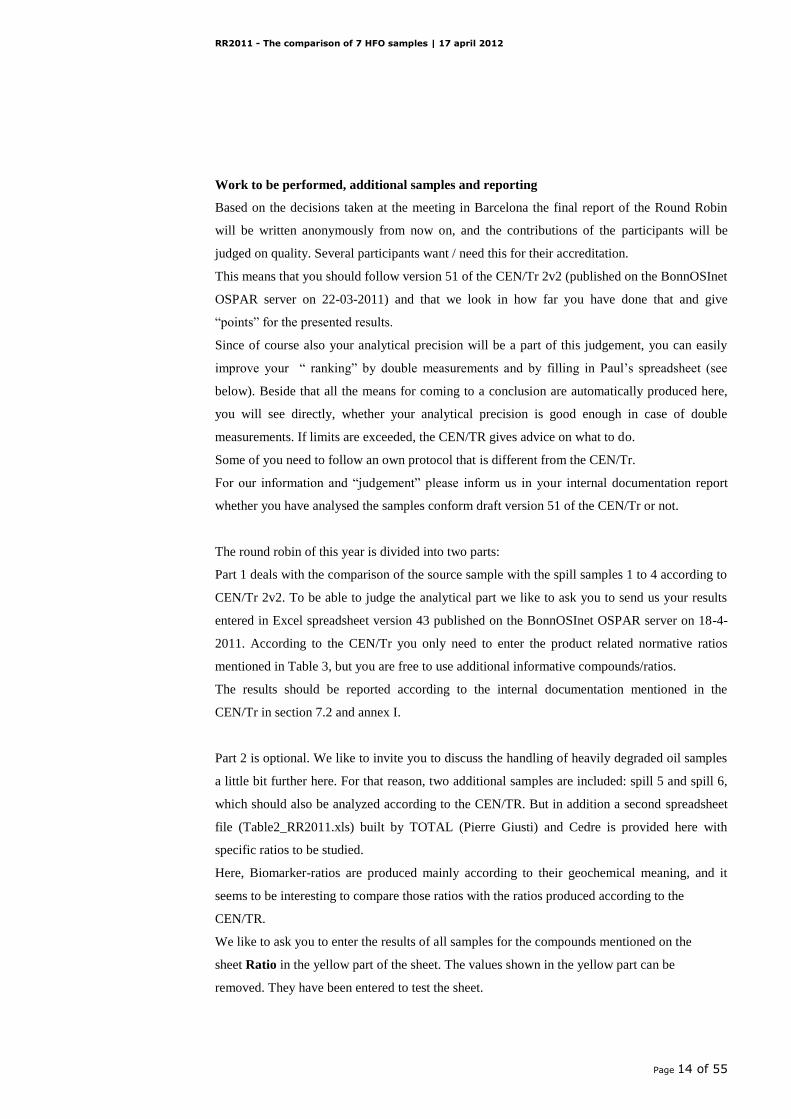
of samples collected either in 2001 or in 2011 is as follows:

2001 Reference oil (source 1)

2001

2001

Oil sampled on a rock (spill 1)

Oil from a contaminated sediment (spill 2)

2011, Tregana Beach

Oil from a contaminated sediment (spill 3),

Oil sampled on a rock (spill 4)

2011, Portez Beach Oil sampled on a rock (spill 5),

Oil from a contaminated sediment (spill 6),

To be able to send all participants the same samples, the oil spill samples have been dissolved in

DCM at a concentration of 100 mg/ml.

NOTE

For literal quotations of

parts of reports,

publications and letters, in

this report the typesetting

of the text to the right is

used

Table 2.1

RR2011 sample composition


Page 14 of 55

Work to be performed, additional samples and reporting

Based on the decisions taken at the meeting in Barcelona the final report of the Round Robin

will be written anonymously from now on, and the contributions of the participants will be

judged on quality. Several participants want / need this for their accreditation.

This means that you should follow version 51 of the CEN/Tr 2v2 (published on the BonnOSInet

OSPAR server on 22-03-2011) and that we look in how far you have done that and give

“points” for the presented results.

Since of course also your analytical precision will be a part of this judgement, you can easily

improve your “ ranking” by double measurements and by filling in Paul’s spreadsheet (see

below). Beside that all the means for coming to a conclusion are automatically produced here,

you will see directly, whether your analytical precision is good enough in case of double

measurements. If limits are exceeded, the CEN/TR gives advice on what to do.

Some of you need to follow an own protocol that is different from the CEN/Tr.

For our information and “judgement” please inform us in your internal documentation report

whether you have analysed the samples conform draft version 51 of the CEN/Tr or not.

The round robin of this year is divided into two parts:

Part 1 deals with the comparison of the source sample with the spill samples 1 to 4 according to

CEN/Tr 2v2. To be able to judge the analytical part we like to ask you to send us your results

entered in Excel spreadsheet version 43 published on the BonnOSInet OSPAR server on 18-4-

2011. According to the CEN/Tr you only need to enter the product related normative ratios

mentioned in Table 3, but you are free to use additional informative compounds/ratios.

The results should be reported according to the internal documentation mentioned in the

CEN/Tr in section 7.2 and annex I.

Part 2 is optional. We like to invite you to discuss the handling of heavily degraded oil samples

a little bit further here. For that reason, two additional samples are included: spill 5 and spill 6,

which should also be analyzed according to the CEN/TR. But in addition a second spreadsheet

file (Table2_RR2011.xls) built by TOTAL (Pierre Giusti) and Cedre is provided here with

specific ratios to be studied.

Here, Biomarker-ratios are produced mainly according to their geochemical meaning, and it

seems to be interesting to compare those ratios with the ratios produced according to the

CEN/TR.

We like to ask you to enter the results of all samples for the compounds mentioned on the

sheet Ratio in the yellow part of the sheet. The values shown in the yellow part can be

removed. They have been entered to test the sheet.


Page 15 of 55

The remaining tables and the graphs on the sheet Figures are based on the data entered in

the yellow part. The sheet Chromato shows chromatograms with the peaks intended.

All the analyses will have to be run in duplicates.

The results of the comparisons can directly be seen in the column diagrams.

Are these “geochemical” ratios better suitable in case of heavily degraded samples?

Or are they even better suitable in all cases?

Time schedule

19-09-11: The samples have been sent out.

Before 1st February 2012: Reports have to be returned.

March: Final report will be sent to the participants.

Meeting: 24-26 April 2011 in France.

On request of some of the participants the final date to send the reports has been moved from

the 1st of November to the 1

st of February. When you have finished your results earlier, don’t

hesitate to send us the results. It gives us more time for the evaluation.

In previous round robins we were quite liberal in accepting reports that were sent in too late.

But we cannot do that with a final date of the 1st of February, so it is a real deadline.

The results should be sent by email to:

Julien.Guyomarch, Ronan.Jezequel; Gerhard.Dahlmann and Paul.Kienhuis.

Yours sincerely,

Julien Guyomarch & Ronan Jezequel, CEDRE.

Pierre Giusti, TOTAL

Paul Kienhuis, RWS-WD

Gerhard Dahlmann, BSH


Page 16 of 55


Page 17 of 55

3 Real scenario

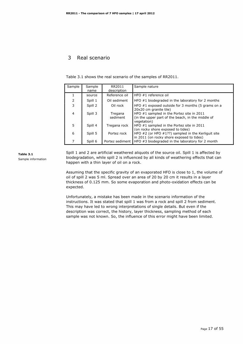
Table 3.1 shows the real scenario of the samples of RR2011.

Sample Sample name

RR2011 description

Sample nature

1 source Reference oil HFO #1 reference oil

2 Spill 1 Oil sediment HFO #1 biodegraded in the laboratory for 2 months

3 Spill 2 Oil rock HFO #1 exposed outside for 3 months (5 grams on a 20x20 cm granite tile)

4 Spill 3 Tregana sediment

HFO #1 sampled in the Portez site in 2011 (in the upper part of the beach, in the middle of vegetation)

5 Spill 4 Tregana rock HFO #1 sampled in the Portez site in 2011 (on rocky shore exposed to tides)

6 Spill 5 Portez rock HFO #2 (or HFO #1??) sampled in the Kerliguit site in 2011 (on rocky shore exposed to tides)

7 Spill 6 Portez sediment HFO #3 biodegraded in the laboratory for 2 month

Spill 1 and 2 are artificial weathered aliquots of the source oil. Spill 1 is affected by

biodegradation, while spill 2 is influenced by all kinds of weathering effects that can

happen with a thin layer of oil on a rock.

Assuming that the specific gravity of an evaporated HFO is close to 1, the volume of

oil of spill 2 was 5 ml. Spread over an area of 20 by 20 cm it results in a layer

thickness of 0.125 mm. So some evaporation and photo-oxidation effects can be

expected.

Unfortunately, a mistake has been made in the scenario information of the

instructions. It was stated that spill 1 was from a rock and spill 2 from sediment.

This may have led to wrong interpretations of single details. But even if the

description was correct, the history, layer thickness, sampling method of each

sample was not known. So, the influence of this error might have been limited.

Table 3.1

Sample information


Page 18 of 55


Page 19 of 55

4 Evaluation of the case following CEN/TR 15522-2v2 v51.

4.1 Preliminary remark

RR2011 was the most difficult inter-calibration we had so far. Generally, the

question arose: how should an analyst decide, whether differences even among the

most stable biomarkers are caused by weathering over ten years or are true

differences? This is not possible by means of the few samples, included in this

Round Robin. As indicated also by several participants, an investigation like this

requires a much higher number of samples, taken continuously over the time of ten

years. Only then, sound conclusions may be possible: depending on the specific

environmental conditions (e.g. oil on rocks or oil in sediments) a homogeneous

distribution cannot be expected as different parts of the spill might alter differently.

Thus, the general trend has to be worked out over the years, and those

inhomogeneous distributions have to be taken into account.

CEDRE has indeed monitored the spill over more than ten years, and from the big

number of analyzed spill samples, only very few were chosen for this Round Robin.

It is indeed interesting to be confronted with highest degrees of weathering of oil

spills.

But with regard to the very limited number of samples, which can be used in our

Round Robins, „the scenario hinders a robust conclusion and it is a matter of

definition (choice?) to conclude a “probable match” or a “non-match”.

Therefore, in this exercise, the way to come to a conclusion must be regarded as

much more important than the conclusion itself. This is especially true because even

the conclusion of a “match” between source and spill samples might have only a

very limited value in a court proceeding, because of many other possibly matching

sources.

Diagrams from the individual reports, which best showed the single steps of the

CEN/TR, were combined in this chapter, together with corresponding interpretations.

In Round Robins like this, a “story” has to be invented because participants should

not know the results, i.e. the actual origin of the samples, from the beginning. On

the other hand, the truth must be known because participants must know, whether

they were right or not with regard to their conclusions.

The story as given here in the “Instructions” seems to be suitable: the two samples

described as “taken one year after the accident”, i.e. spill 1 and spill 2, were

actually samples taken from the spill, but they were artificially weathered. The right

conclusion is thus a match with the source sample 1. The next two samples

described as “taken 10 years after the accident”, where indeed taken after 10

years, and they indeed originate from source 1. This was ensured by CEDRE by

continuous sample taking on the same location over this long time. Spill 6 originates

from another accident, where also long time investigations have been carried out.

Merely the origin of spill 5 is not clear, and CEDRE has used the opportunity of this

Round Robin to get the opinions about this sample from different laboratories from

all over the world.


Page 20 of 55

4.2 GC-FID

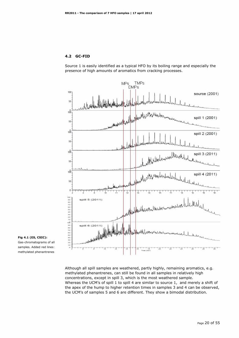
Source 1 is easily identified as a typical HFO by its boiling range and especially the

presence of high amounts of aromatics from cracking processes.

Although all spill samples are weathered, partly highly, remaining aromatics, e.g.

methylated phenantrenes, can still be found in all samples in relatively high

concentrations, except in spill 3, which is the most weathered sample.

Whereas the UCM’s of spill 1 to spill 4 are similar to source 1, and merely a shift of

the apex of the hump to higher retention times in samples 3 and 4 can be observed,

the UCM’s of samples 5 and 6 are different. They show a bimodal distribution.

Fig 4.1 (ES, CSIC):

Gas-chromatograms of all

samples. Added red lines:

methylated phenantrenes


Page 21 of 55

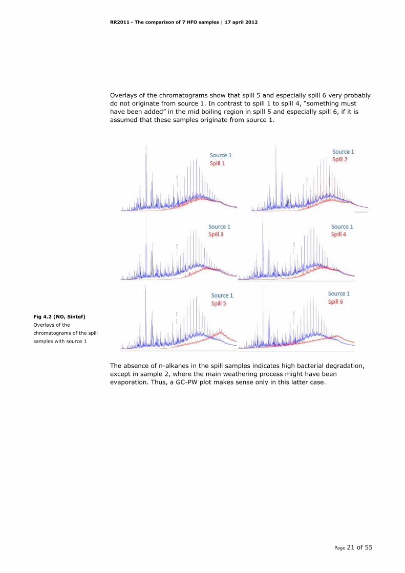
Overlays of the chromatograms show that spill 5 and especially spill 6 very probably

do not originate from source 1. In contrast to spill 1 to spill 4, “something must

have been added” in the mid boiling region in spill 5 and especially spill 6, if it is

assumed that these samples originate from source 1.

The absence of n-alkanes in the spill samples indicates high bacterial degradation,

except in sample 2, where the main weathering process might have been

evaporation. Thus, a GC-PW plot makes sense only in this latter case.

Fig 4.2 (NO, Sintef)

Overlays of the

chromatograms of the spill

samples with source 1


Page 22 of 55

PW-plot RR2011 spill 2 vs source 1

0

20

40

60

80

100

120

5 10 15 20 25 30 35

n-alkane number

Re

ma

inin

g a

mo

un

t, %

2

isopren

The GC-PW plot of spill 2 versus source 1 points to a possible match: a typical S-

shaped evaporation curve can be found. Pristane and phytane are in line with this

curve. There is thus no indication of biodegradation.

4.3 GC-MS

4.3.1 First visual inspection

All samples consist of HFO: They show the typical mass-chromatograms of HFO

including the typical pattern of the methylphenanthrenes and the absence of retene.

Methylanthracene is present in the typical higher concentration except for spill 3 and

6, which can have been caused by weathering here.

Besides retene, 30O is not present, except may be in spill 6 in very low amount.

SC26TA shows a too low S/N-ratio, except in spill 6 and spill 7.

4.3.2 Spill 1- source 1

As found already by GC-FID, also the MS-PW-plot of Fig. 4 shows that sample Spill 1

was affected by weathering when compared to sample Source 1. The complex

pattern combines the effects of evaporation, biodegradation, and dissolution. The

presence of pristane and phytane and the absence of C17 and C18 and of all further

n-alkanes indicates that biodegradation has occurred.

The C1-fluoranthenes/pyrenes/benzofluorenes (m/z 216) pattern has been affected

by dissolution and/or biodegradation. In this case, the compounds 2-

methylfluoranthene and the two benzofluorenes were more reduced than the methyl

pyrenes.

The compounds eluting after a retention time of 42 min are above 85% and have

not been affected by weathering. These include both normative and informative

biomarkers. The similar relative concentration of biomarkers is an indication of same

source.

Fig 4.3 (SE, SKL)

GC-PW plot spill 2 versus

source 1


Page 23 of 55

“Unknown” peaks appear in m/z 198 originating from fragments of other

compounds, e.g. alkanes:

As TMPhen is also reduced in spill 1 by dissolution and/or biodegradation, the stable

biomarkers are shifted to the 130-140% line, when the PW-plot is based on TMPhen

(Fig. 5).

A final visual inspection of all mass-chromatograms shows a high similarity between

source 1 and spill 1.

Conclusion:

There is no significant difference between spill 1 and source 1: positive match.

Fig 4.4

MS-PW-plot and DR

comparison graph

spill 1 - source 1.

Fig 4.5

MS-PW-plot spill 1 - source

1, based on TMPhen.


Page 24 of 55

4.3.3 Spill 2 – source 1

As already was found in GC-FID and in the GC-PW-plot, spill 2 shows high

evaporative loss of compounds up to about 40 minutes. But n-alkanes are still

present, and the GC-PW plot shows a match situation (Fig. 3).

The C1-fluoranthenes/pyrenes/benzofluorenes (m/z 216) show a strong reduction in

intensity. For C1-pyrenes, the degradation pattern was 1-MPy (PW: 23%) > 4-MPy

(PW: 40%) >2-MPy (PW: 44%). Benzo(b+c)fluorene and benzo(a)fluorene have

been remarkably reduced. These effects must especially be attributed to photo

oxidation.

But the most remarkable feature of spill 2 is the reduction of the triaromatic

steranes to about 70%.

TAS are among the compounds most resistant to biodegradation.

But biodegradation has hardly occurred in spill 2 because high n-alkanes are still

present, and pristane and phytane are in line with the S-shaped evaporation curve

of the n-alkanes.

As belonging to the PAHs, TAS might have been affected in spill 2 in the same way

as the other aromatics, i.e. by dissolution and especially by photo oxidation. This is

in accordance with the strong effect of photo oxidation on the compounds of m/z

216 in this sample (see above).

It is worth to notice here that the TAS are effected nearly equally. This means that

the differences of the DRs produced from the TAS are very well below the

repeatability limit of 14%, when spill 2 is compared to source 1.

A final visual inspection of all mass-chromatograms shows a very high similarity

between spill 2 and source 1.

Taking all this information into account, it can be concluded:

Fig 4.6

MS-PW-plot and DR

comparison graph spill 2 -

source 1.


Page 25 of 55

Conclusion:

There is no significant difference between spill 2 and source 1: positive match.

4.3.4 Spill 3 and spill 4 – source 1

It is not astonishing that highest weathering effects occur in 10 year old samples,

and the interpretation of the analytical results would be much easier, if samples

taken continuously over this long time were present. In this Round Robin, we can

only compare the samples we have. But it might be a good idea also to compare the

spill samples among each other.

As found already in the comparison of the GCs (Fig. 1 and 2) the MS-PW-plots show

increased weathering in spills 3 and 4. With regard to these weathering effects,

discussed already, when spills 1 and 2 are compared to source 1, the following

range can be observed:

spill 1 < spill 2 < spill 4 < spill 3. These include evaporation and biodegradation in

spill 1, evaporation in spill 2, and the reduction of the aromatics by dissolution and

photo oxidation.

The same reduction of the TAS as in spill 2 can be observed in spills 4 and 3,

whereas these compounds are more spread in spill 3. Spill 3 is the most weathered

sample, and if a match is assumed with source 1, this can only be explained by

additional biodegradation. Correspondingly, the differences of the DRs produced

from these TAS are above the repeatability limit, when spill 3 is compared to source

1.

Fig 4.7 (DE, BSH)

MS-PW-plots spills 1 to 4

based on source 1


Page 26 of 55

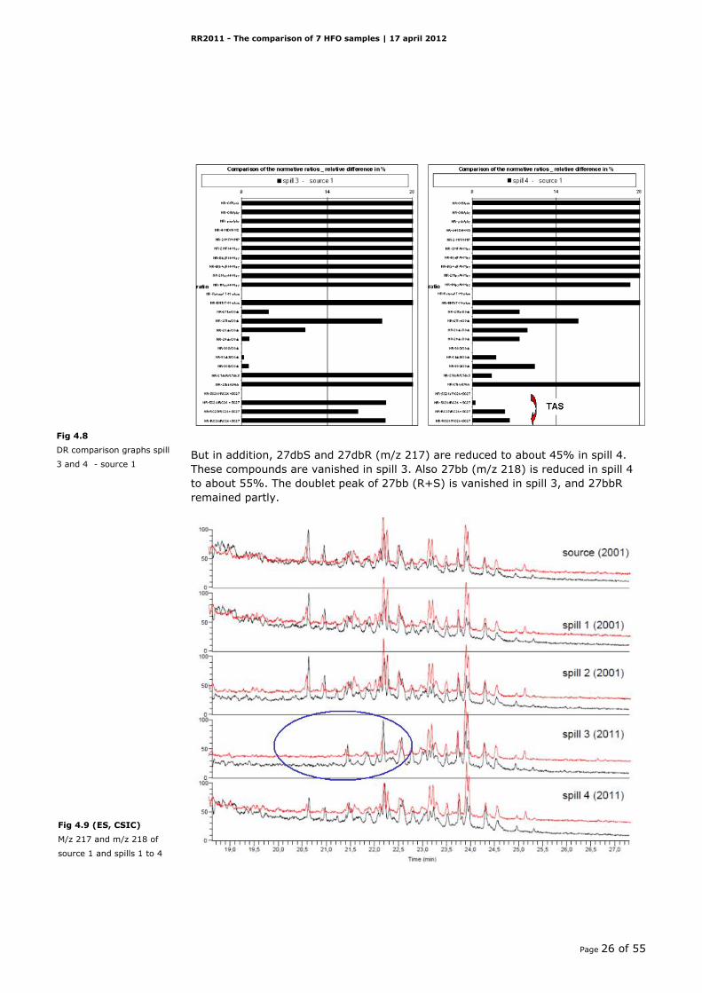
But in addition, 27dbS and 27dbR (m/z 217) are reduced to about 45% in spill 4.

These compounds are vanished in spill 3. Also 27bb (m/z 218) is reduced in spill 4

to about 55%. The doublet peak of 27bb (R+S) is vanished in spill 3, and 27bbR

remained partly.

Fig 4.8

DR comparison graphs spill

3 and 4 - source 1

Fig 4.9 (ES, CSIC)

M/z 217 and m/z 218 of

source 1 and spills 1 to 4


Page 27 of 55

Beside those differences, the visual inspection of the mass-chromatograms still

shows a high similarity between source 1 and spills 4 and 3.

Some differences are the same as found between spills 1, 2 and source 1 and could

be explained here uniquely. The fact that there is a chain from source 1 over spill 1

and 2 and especially spill 4 to spill 3 makes it highly probable that spill 4 and also

spill 3 originate from source 1.

Conclusion:

Spill 3 and source 1: probable match

Spill 4 and source 1: probable match


Page 28 of 55

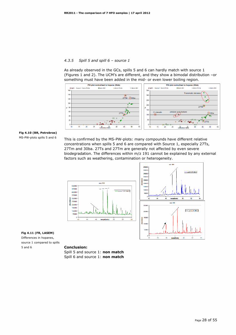
4.3.5 Spill 5 and spill 6 – source 1

As already observed in the GCs, spills 5 and 6 can hardly match with source 1

(Figures 1 and 2). The UCM’s are different, and they show a bimodal distribution –or

something must have been added in the mid- or even lower boiling region.

This is confirmed by the MS-PW-plots: many compounds have different relative

concentrations when spills 5 and 6 are compared with Source 1, especially 27Ts,

27Tm and 30ba. 27Ts and 27Tm are generally not affected by even severe

biodegradation. The differences within m/z 191 cannot be explained by any external

factors such as weathering, contamination or heterogeneity.

Conclusion:

Spill 5 and source 1: non match

Spill 6 and source 1: non match

Fig 4.10 (BR, Petrobras)

MS-PW-plots spills 5 and 6

Fig 4.11 (FR, LASEM)

Differences in hopanes,

source 1 compared to spills

5 and 6


Page 29 of 55

5 Common aspects of the reports

In this chapter some general issues are discussed. For the judgement of the

individual reports see chapter 7.

5.1 Sample treatment

In the CEN/Tr section 5.4.1 it is strongly advised to clean “black” samples over silica

or florisil before analyses. From the scenario it can be concluded that the samples

contain a high boiling fraction that is resistant against weathering for more than 10

years. The clean-up is used to remove the high amount of asphaltenes and/ or

particles that do not leave the column and influence the column performance.

Table 5.1 shows that not all participants have cleaned the samples before injection.

injection injection

Lab code Clean-up concentration volume

mg/ml µl

Lab1 no 10 1

Lab2 no 5 1

Lab3 no 2 FID_20 MS n.a.

Lab4 yes 1 n.a.

Lab5 n.a. n.a. n.a.

Lab6 n.a. 5 1

Lab7 no 5 or 10 n.a.

Lab8 yes 5 1

Lab9 yes n.a. n.a.

Lab10 no 20 n.a.

Lab11 yes 20 1

Lab12 no 10 1

Lab13 n.a. n.a. n.a.

Lab14 no 2.5 1


Lab16 yes 5 1

Lab17 yes 5 3


Lab19 yes 3 1

A “yes” for the clean-up has been indicated when it was mentioned in the report. A

“no” was concluded when e.g. in the report it was mentioned that the samples were

diluted before injection without mentioning the clean-up step. Some reports did not

describe the sample treatment at all. The information could also not been found in

the spreadsheet file. This is indicated with n.a.

The injection concentration varies from 1 to 20 mg/ml. Basically the amount of oil

should not be more than needed to receive reliable data. Small peaks should be

seen, while the higher peaks should not be overloaded.

Table 5.1

Sample clean-up and

injection volume and

concentration.

n.a. = not available.


Page 30 of 55

Specific for the heavily weathered samples of the ring test is that the alkanes are

not present. For such samples it is advised to inject such an amount that the peak

height of the hopanes is at the level of the hopanes in the source sample.

5.2 Variance of the duplicate analyses of the source sample

Table 5.2 shows the variance of the duplicate analyses of the source sample. The

data are retrieved from two tables in the spreadsheet file v43 available on the

BonnOSInet web server.

The MS-PW-plot variance can be found in cell AE82 of each comparison sheet. This

table has been used for the evaluation of the PW-plot of RR2009 and more

information can be found in section 5.2 of the summary report of RR2009.

The st. deviation of the paired ratios [1] can be found in the Table belonging to cell

A104 of each comparison sheet. First the ratios that have been analyzed should be

selected in column G (1 = taken into account and empty= not taken into account).

The st. dev. can be calculated separately for the normative and informative ratios.

So Table 5.2 shows also how many of the ratios have been used by each lab.

MS-PW-plot Number and st. dev. of the paired ratios

Lab code Normalized to hopane Normative ratios

Informative ratios

all ratios

mean St. dev. Number St dev Number St dev Number St dev

Lab1 105 5.3 24 5.5 12 3.8 36 5.0

Lab2 97 2.7 17 2.7 6 0.9 23 2.3

Lab3 107 7.4 20 3.1 11 2.9 31 3.0

Lab4 104 3.4 23 3.2 6 3.4 29 3.2

Lab5 121 19.0 24 3.1 24 3.1

Lab6 101 9.5 22 5.8 5 3.3 27 5.4

Lab7 96 4.0 22 3.4 4 2.1 26 3.3

Lab8 96 4.0 22 4.7 6 2.9 28 4.3

Lab9 95 7.3 8 3.1 3 1.2 11 2.7

Lab10 108 14.3 24 4.2 24 4.2

Lab11 103 4.6 24 3.9 12 2.8 36 3.6

Lab12 106 11.6 24 5.6 6 2.9 30 5.2

Lab13 109 6.5 24 4.0 12 3.4 36 3.8

Lab14 101 4.8 25 3.1 12 4.4 37 3.6

Lab15 100 12.1 25 6.3 25 6.3

Lab16 99 4.3 21 3.3 21 3.3

Lab17 101 5.5 22 3.5 22 3.5

Lab18 n.r. n.r. n.r. n.r. n.r. n.r. n.r. n.r.

Lab19 93 3.0 22 3.2 6 4.1 28 3.4

In the summary report of RR2009 it was concluded that a reasonably value for the

st. dev of the MS-PW-plot would be 7 to 8%. Table 5.2 shows that most of the

participants were able to stay below that value.

The highest value was found for lab 5, while the st. dev of their ratio comparison is

3.1, much lower than the accepted limit of 5%. The higher value is related to a

“drifting” of the data points of the MS-PW-plot.

Table 5.2

Variance of the MS-PW-plot

and the combined ratios by

means of a paired

calculation of the st. dev of

the ratios.

Pw-plot >7 in bold

Ratios > 4.5 in bold


Page 31 of 55

Lab 5 MS-PW-plot Number and st. dev of the paired ratios

Normalized to hopane Normative Informative all ratios

mean St. dev Number St dev Number St dev Number St dev

source 121 19.0 24 3.1 spill 1 99 2.7 24 2.2 spill 2 124 15.0 24 4.1

Table 5.3.shows that the results for spill 1 are much better but for spill 2 again very

high for the MS-PW-plot. The reason is unknown.

Lab 10 has also a higher variance for the MS-PW-plot. Their report indicated that

the duplicate sequence was analyzed one week later, which has probably caused the

high variance of the PW plot. The variance of the ratios however is less sensible for

the difference of one week in analysis.

The duplicate analyses of some to all of the samples is used to check the quality of

the data and also to eliminate ratios with a higher variance (see sections 6.4.3 and

6.5.6.3 of the CEN/Tr). It is strongly advised to perform these steps to check the

data quality and to be able to eliminate ratios with a higher variance.

5.3 Oil type recognition.

Table 5.4 shows the oil type indication found in the reports.

source spill 1 spill 2 spill 3 spill 4 spill 5 spill 6

Lab1 n.m. n.m. n.m. n.m. n.m. n.m. n.m.

Lab2 HFO HFO HFO HFO HFO HFO HFO


Lab4 HFO HFO HFO HFO HFO HFO/crude HFO





Lab9 n.p. n.p. n.p. n.p. n.p. n.p. n.p.



Lab12 HFO HFO HFO n.m. HFO n.m. n.m.


Lab14 HFO HFO HFO HFO HFO n.m. n.m.


Lab16 HFO HFO HFO/crude n.p. HFO HFO/crude HFO


Lab18 n.r. n.r. n.r. n.r. n.r. n.r. n.r.


Most of the participants reported that the samples contained heavy fuel oil (HFO).

Lab 9 reported that an indication was not possible because of the severe

weathering. Several labs reported the oil type only for those samples that were not

Table 5.3

St dev of the MS-PW-plot

and ratio comparison of Lab

5 for also spill 1 and spill 2

Table 5.4

Oil type recognition:

n.m. = not mentioned

n.p. = not possible

n.r. = no report received


Page 32 of 55

too weathered (indicated with n.p. = not possible) or indicated some samples with

an HFO/crude because the C1-phenantrenes pattern was changed too much.

Some labs just started with the sample comparison without mentioning the oil type.

This is indicated with n.m. (not mentioned)

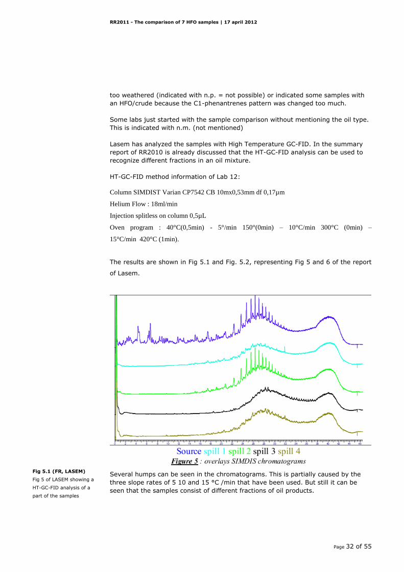
Lasem has analyzed the samples with High Temperature GC-FID. In the summary

report of RR2010 is already discussed that the HT-GC-FID analysis can be used to

recognize different fractions in an oil mixture.

HT-GC-FID method information of Lab 12:

Column SIMDIST Varian CP7542 CB 10mx0,53mm df 0,17µm

Helium Flow : 18ml/min

Injection splitless on column 0,5µL

Oven program : 40°C(0,5min) - 5°/min 150°(0min) – 10°C/min 300°C (0min) –

15°C/min 420°C (1min).

The results are shown in Fig 5.1 and Fig. 5.2, representing Fig 5 and 6 of the report

of Lasem.

Several humps can be seen in the chromatograms. This is partially caused by the

three slope rates of 5 10 and 15 °C /min that have been used. But still it can be

seen that the samples consist of different fractions of oil products.

Fig 5.1 (FR, LASEM)

Fig 5 of LASEM showing a

HT-GC-FID analysis of a

part of the samples


Page 33 of 55

Fig 5.2 shows that spill 5 and spill 6 are very different from the source sample but

also different between themselves. Weathering might have had an effect but the

difference in the HT part is very likely caused by a difference in composition.

The chromatogram of Spill 3 is remarkable. The sample comparison, see section

4.3.4 showed that the sample is more weathered than sample 4 which can explain

the difference in UCM of the first hump compared with the source sample. The

retention time section from 32 to 38 min shows however differences in shape and

an n-alkane pattern that is not present in the source sample.

This extra range of alkanes is also shown in Fig 5.3.

Fig 5.2 (FR, LASEM)

Fig 6 of LASEM showing a

HT-GC-FID analysis of a

part of the samples


Page 34 of 55

- Alkanes m/z 85

46.00 48.00 50.00 52.00 54.00 56.00 58.00 60.00 62.00 64.000

170000

Time-->

AbundanceIon 85.00 (84.70 to 85.70): C1100504.D\data.ms

46.00 48.00 50.00 52.00 54.00 56.00 58.00 60.00 62.00 64.000

12500

Time-->


46.00 48.00 50.00 52.00 54.00 56.00 58.00 60.00 62.00 64.000

180000

Time-->


46.00 48.00 50.00 52.00 54.00 56.00 58.00 60.00 62.00 64.000500

13000

Time-->


46.00 48.00 50.00 52.00 54.00 56.00 58.00 60.00 62.00 64.000

40000

Time-->


46.00 48.00 50.00 52.00 54.00 56.00 58.00 60.00 62.00 64.000

52000

Time-->


46.00 48.00 50.00 52.00 54.00 56.00 58.00 60.00 62.00 64.000

23000

Time-->


Height hopane

47.618

Height hopane

48.433

Height hopane

53.046

Height hopane

67.403

Height hopane

67.325

Source

2001

Spill 1

Rock 2001

Spill 2

Sediment 2001

Spill 3

Sediment 2011

Spill 4

Rock 2011

Spill 5

Rock 2011

Spill 6

Sediment 2011

Height hopane

92.564

Height hopane

72.264

C34

C36

C32 C38

It suggests oil from a different source or a contamination of the weathered source 1.

Redistribution of the alkanes as weathering process is unlikely because the source

barely contains alkanes in this range.

Fig 5.3 (NL, RWS-WD)

Comparison of the samples

for m/z 85 representing the

alkanes


Page 35 of 55

5.4 Normative compound/ratio exclusion

Table 5.5 shows that participants have excluded normative ratios differently. In

section 6.5.3 of the CEN/TR one can find that the exclusion of normative ratios

should be conducted carefully, and reasons should be mentioned in the technical

report. Not all participants followed this advice. Information about this point was

found partly in the reports and partly in the spreadsheet files. It is possible that a

lab integrates all normative compounds and eliminates ratios for comparison based

on the results of the duplicate comparison while the integration results can still be

found in the spreadsheet file. We found however no indication of this procedure in

the reports.

Retene is normally not present in HFO. This can be found in Table 3 of the CEN/Tr.

Retene elutes together with the C4-phenantrenes (m/z 234) and it is sometimes

difficult to see whether it is present or not. Checking the presence of fragment ion

m/z 219 helps to recognize it properly, see Fig E.2 of the CEN/Tr.

The other peaks SC26TA, 30O and 28ab are on a very low level or absent in the

samples. 30O is only present at a little bit higher level in spill sample 5.

NR-retene NR-SC26TA NR-30O 28ab

Lab1 no yes yes yes

Lab2 no no no no

Lab3 no no no no

Lab4 no yes no yes

Lab5 yes yes no yes

Lab6 no no no yes

Lab7 no no no yes

Lab8 no no no yes

Lab9 no no no no

Lab10 yes yes no yes

Lab11 yes yes yes yes

Lab12 no no no no





Lab17 no no no no


Lab19 no yes no no

5.5 Informative compound integration.

The comparison spreadsheet used to generate the PW-plots and to compare the

ratios, also contains a range of informative ratios that can be used, depending on

the type of samples, to generate extra information about the weathering of

Table 5.5

Normative ratios excluded /

included by the participants.


Page 36 of 55

compounds and the similarity of samples. Table 5.2 shows that 13 labs have used a

part to most of these ratios.

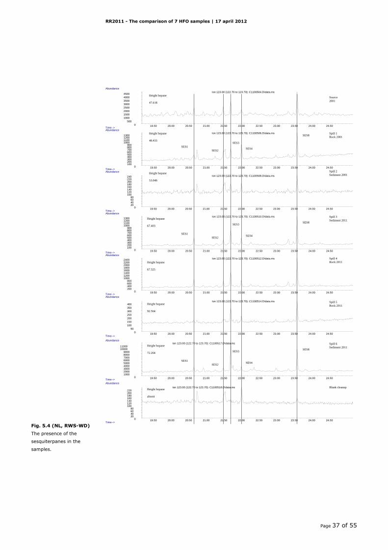
Among these compounds are the sesquiterpanes, see Fig 5.4. These compounds

have a low boiling point and thus easily evaporate but are very stable against other

weathering effects like biodegradation and photo-oxidation.

According to the real scenario spill 1 is an aliquote of the source sample that is

biodegraded for 3 months at the lab, spill 2 an aliquote of the source that has been

weathered on a tile for three months.

Both spill samples show a clear pattern of the sesquiterpanes. The pattern of the

source sample is however disturbed by a high background. The baseline of the

source sample is at a level of 1500, while the baseline of the blanc is at a level of

140. This background is caused by the high number of lighter compounds in this

section of the chromatogram, which generate m/z 123 as fragment ion.

In spill samples 1 and 2 this background is strongly reduced.

Together with the partly evaporation of the sesquiterpanes it is difficult to use this

information for comparing the samples. Spill sample 6 is an exception because it can

be seen that SES4 is higher than SES 8 in spill 6 while it is lower than SES 8 in spill

samples 1 and 2. This cannot be caused by evaporation and is a real difference.

The blanc that underwent a cleanup shows besides a low baseline also some peaks

of which two coelute with resp SES 4 and SES 8. SES 8 is used in the PW-plots

shown in section 7 and the data are reliable because the peak height of the pek in

the blanc is neglectable compared with the peak heights in the source and spill

samples.

Besides the sesquiterpanes also decalin and the C1-dekalins are present in the

samples. These compounds have the same weathering behaviour as the

sesquiterpanes and can be used as weathering markers in the MS-PW-plots.


Page 37 of 55

Sesquiterpanes

19.50 20.00 20.50 21.00 21.50 22.00 22.50 23.00 23.50 24.00 24.500

500

1000

1500

2000

2500

3000

3500

4000

4500

Time-->

Abundance

Ion 123.00 (122.70 to 123.70): C1100504.D\data.ms

19.50 20.00 20.50 21.00 21.50 22.00 22.50 23.00 23.50 24.00 24.500100200300400500600700800900

1000110012001300

Time-->


19.50 20.00 20.50 21.00 21.50 22.00 22.50 23.00 23.50 24.00 24.500

20406080

100120140160180200220240

Time-->

Abundance

Ion 123.00 (122.70 to 123.70): C1100508.D\data.ms

19.50 20.00 20.50 21.00 21.50 22.00 22.50 23.00 23.50 24.00 24.500100200300400500600700800900

1000110012001300

Time-->


19.50 20.00 20.50 21.00 21.50 22.00 22.50 23.00 23.50 24.00 24.500200400600800

10001200140016001800200022002400

Time-->

Abundance

Ion 123.00 (122.70 to 123.70): C1100512.D\data.ms

SES1

SES2

SES3

SES4

SES8

Height hopane

47.618

Height hopane

48.433

Height hopane

53.046

Height hopane

67.403

Height hopane

67.325

Source

2001

Spill 1

Rock 2001

Spill 2

Sediment 2001

Spill 3

Sediment 2011

Spill 4

Rock 2011

19.50 20.00 20.50 21.00 21.50 22.00 22.50 23.00 23.50 24.00 24.500

50

100

150

200

250

300

350

400

Time-->

Abundance

Ion 123.00 (122.70 to 123.70): C1100514.D\data.ms

19.50 20.00 20.50 21.00 21.50 22.00 22.50 23.00 23.50 24.00 24.500100020003000400050006000700080009000

1000011000

Time-->


19.50 20.00 20.50 21.00 21.50 22.00 22.50 23.00 23.50 24.00 24.500

20406080

100120140160180200220

Time-->

Abundance

Ion 123.00 (122.70 to 123.70): C1100518.D\data.ms

Spill 5

Rock 2011

Spill 6

Sediment 2011

Blank cleanup

Height hopane

92.564

Height hopane

72.264

Height hopane

absent

SES1

SES2

SES3

SES4

SES8

SES1

SES2

SES3

SES4

SES8

Fig. 5.4 (NL, RWS-WD)

The presence of the

sesquiterpanes in the

samples.


Page 38 of 55

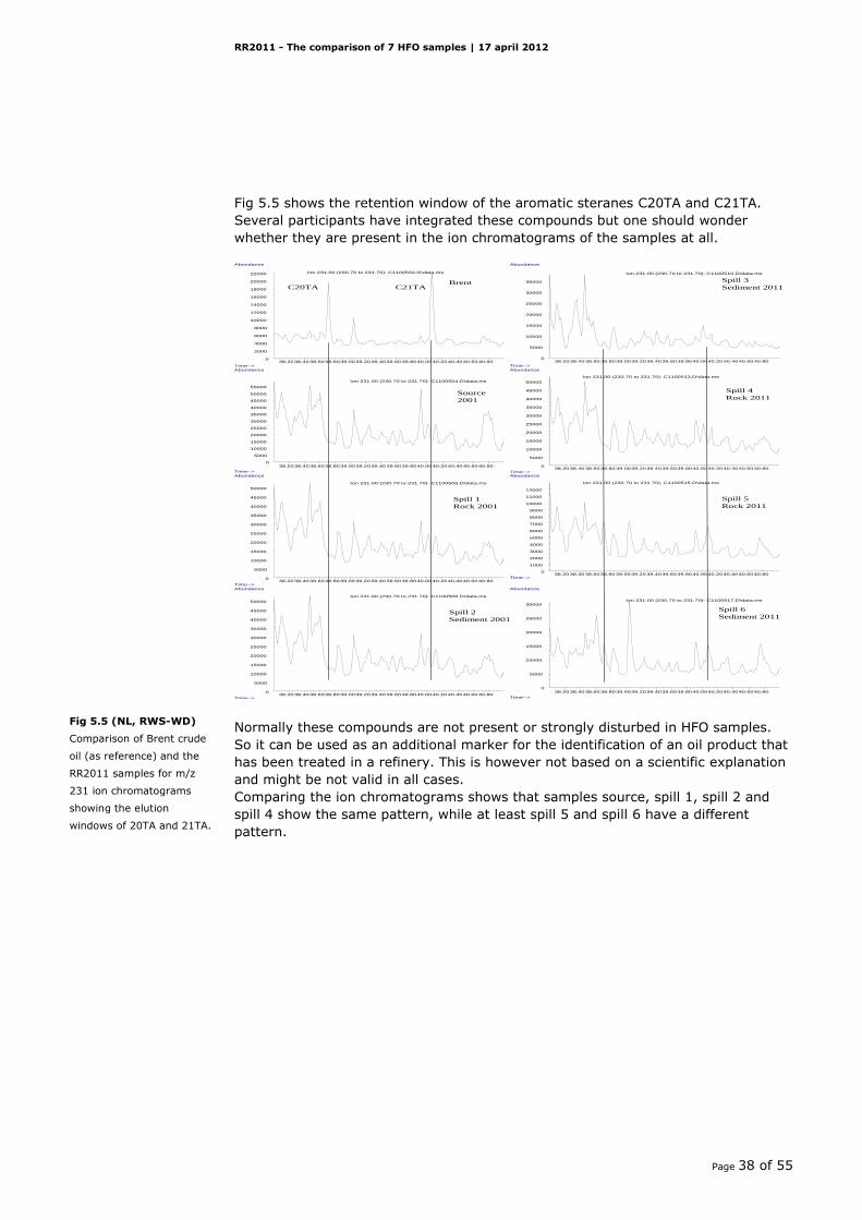
Fig 5.5 shows the retention window of the aromatic steranes C20TA and C21TA.

Several participants have integrated these compounds but one should wonder

whether they are present in the ion chromatograms of the samples at all.

38.2038.4038.6038.8039.0039.2039.4039.6039.8040.0040.2040.4040.6040.800

5000

10000

15000

20000

25000

30000

Time-->

Abundance

Ion 231.00 (230.70 to 231.70): C1100517.D\data.ms

38.2038.4038.6038.8039.0039.2039.4039.6039.8040.0040.2040.4040.6040.800

5000

10000

15000

20000

25000

30000

35000

Time-->

Abundance

Ion 231.00 (230.70 to 231.70): C1100510.D\data.ms

38.2038.4038.6038.8039.0039.2039.4039.6039.8040.0040.2040.4040.6040.800

5000

10000

15000

20000

25000

30000

35000

40000

45000

50000

Time-->

Abundance

Ion 231.00 (230.70 to 231.70): C1100513.D\data.ms

38.2038.4038.6038.8039.0039.2039.4039.6039.8040.0040.2040.4040.6040.800

5000

10000

15000

20000

25000

30000

35000

40000

45000

50000

Time-->

Abundance

Ion 231.00 (230.70 to 231.70): C1100506.D\data.ms

38.2038.4038.6038.8039.0039.2039.4039.6039.8040.0040.2040.4040.6040.800

2000

4000

6000

8000

10000

12000

14000

16000

18000

20000

22000

Time-->

Abundance

Ion 231.00 (230.70 to 231.70): C1100502.D\data.ms

38.2038.4038.6038.8039.0039.2039.4039.6039.8040.0040.2040.4040.6040.800

5000

10000

15000

20000

25000

30000

35000

40000

45000

50000

Time-->

Abundance

Ion 231.00 (230.70 to 231.70): C1100506.D\data.ms

38.2038.4038.6038.8039.0039.2039.4039.6039.8040.0040.2040.4040.6040.800

5000

10000

15000

20000

25000

30000

35000

40000

45000

50000

55000

Time-->

Abundance

Ion 231.00 (230.70 to 231.70): C1100504.D\data.ms

C20TA and C21TA 231

Source

2001

Spill 1

Rock 2001

Spill 2

Sediment 2001

Spill 3

Sediment 2011

Spill 4

Rock 2011

Spill 5

Rock 2011

Spill 6

Sediment 2011

Brent

38.2038.4038.6038.8039.0039.2039.4039.6039.8040.0040.2040.4040.6040.800

1000

2000

3000

4000

5000

6000

7000

8000

9000

10000

11000

12000

Time-->

Abundance

Ion 231.00 (230.70 to 231.70): C1100515.D\data.ms

C20TA C21TA

Normally these compounds are not present or strongly disturbed in HFO samples.

So it can be used as an additional marker for the identification of an oil product that

has been treated in a refinery. This is however not based on a scientific explanation

and might be not valid in all cases.

Comparing the ion chromatograms shows that samples source, spill 1, spill 2 and

spill 4 show the same pattern, while at least spill 5 and spill 6 have a different

pattern.

Fig 5.5 (NL, RWS-WD)

Comparison of Brent crude

oil (as reference) and the

RR2011 samples for m/z

231 ion chromatograms

showing the elution

windows of 20TA and 21TA.


Page 39 of 55

6 Table 2 evaluation

The participants were asked to enter results in a second spreadsheet file called

“Table 2”. The table makes use of ratios based on biomarkers.

R1 27Ts/27Tm (DR-27)

R2 27Ts/30ab

R3 29ab/30ab (DR-29ab)

R4 30d/30ab

R5 31abS/31abR

R6 31abS/30ab

R7 (27dbS + 27dbR)/28aaR

R8 29aaS/29aaR (DR-29aaS)

R9 27bb(R+S)/[28bb(R+S)+29bb(R+S)] (DR-27bbSTER)



R12 [(RC26TA+SC27TA) + SC28 TA] / RC28TA

Table 2 was made by Cedre and Total to test whether it is useful to add (some) of

these ratios to the normative/informative ratios listed in the CEN/Tr.

The report of Total discusses and compares both methods:

Evaluation according the CEN/Tr

When using the guidelines and comparative tables described in the technical report CEN15522,

it can be stated that:

- Extraction of specific hydrocarbons ions such as m/z=85, 191, 192, 198, 216, 217 and 218

show that the 4 samples (SPILL 1 to SPILL 4) are in the same boiling range (hydrocarbon cut)

than the source.

- The height of the normal-paraffin C17 and C18 versus the height of pristane (C19H40) and

phytane (C20H42) proved that the 4 spill samples are biodegraded.

Therefore, in order to correctly compare source and spill sample, only the biomarkers ratios

should and will be used. The comparison of the different biomarkers ratios, shows that spill 1

and spill 2 have an common origin with source 1 (no ratio is over 14%) and that spill 3 and spill

4 have a different origin than source 1 (several ratio are over 28 %)

Conclusion: In accordance with the technical report CEN15522, it can be stated that the

samples Spill 1 and Spill 2 are very biodegraded spills, which have the same origin than the

source 1. On the other hand, Spill 3 and Spill 4 have a different origin than source 1.

Evaluation according Table 2

The second part of the RR2011 takes into account more specific diagnostics ratios of

biomarkers in order to provide some information about the biodegradability level.


Page 40 of 55

Ratios R7, R9, R10 and R11 (pointed in table 2) are not recommended ones in the Technical

Report CEN15522, because these ratios are known to be affected by the biodegradation. For

this reason, associated values from these 4 ratios can be used to estimate the biodegradability

level.

After having checked and proved that the 12 ratios are stable by duplicated measurements in

each sample (delta <14%), the comparison of the 6 spills samples 12 ratios with the source ones

lead to the conclusion that:

- Spill 1 and Spill 2 have a common origin with Source 1

- Spill 3 and Spill 4 have a nearly common origin with Source 1 (without taking into account

the 4 “biodegradation-level-ratios”). Solely a few ratios are between 14 and 28 %.

- Spill 3 seems to be a sample with a very advanced level of the biodegradation (absence of the

following steranes : « 27dbS : 13(H),17(H),20S-cholestane » et « 27dbR : 13(H),17(H),20R-

cholestane »),

- Spill 5 and Spill 6 have a clear different origin than the source 1 : 3 ratios other that R7, R9,

R10 and R11 overrun the 28% barrier)

Conclusion: when using comparative ratios adapted to old spills, it can be stated that Spills 1

and 2 are clearly the same origin than Source1. Spills 3 and 4 have probably the same origin

that source 1 but are very biodegraded and Spills 5 and 6 are coming from a different source.

Table 2 however didn’t help the participants very much in finding a conclusion for

the comparison of spill 3 and spill 4 with Source 1. Many participants where

“confused” by the severe weathering of the 10 years old samples and concluded an

inconclusive or non-match. But still six reported a probable match for the relation

between spill 3-source 1 and nine for the relation between spill 4 – source 1 based

on the CEN/Tr.

This can be explained by the Cen/Tr approach that all sample information should be

compared and not only the biomarkers. See chapter 9 for a discussion about this

issue.

The samples of RR2011 and Table 2 however indicates that information about the

effects of severe weathering, reducing even some of the biomarkers, is missing in

the current version of the CEN/Tr.


Page 41 of 55

7 Evaluation of the weathering of oil by IMOF.

7.1 IMOF

Jan Christensen presented at the meeting in Brest the IMOF method based on

Principle Component Analyses (PCA) [10.3]. The method uses whole ion

chromatograms as base for evaluation.

The presentations of Jan and Fabiana Gallota (BR, Petrobras) dealing with IMOF can

be found on the BonnOSInet server for the participants of the round robin and on

request for others. Some highligths from the presentation of Jan dealing with the

weathering of the PAH’s of the RR2011 samples will be discussed here.

The PCA plot of the RR2011 samples based on 8 ion chromatograms representing

the PAH’s is shown in Fig 7.1

The crosses in the middle of the plot are the result of 16 analyses of a Brent

standard analysed in a period of two years. Also each RR2011 sample is analysed in

duplicate. Both types of data sets indicate the variance caused by the GC-MS

analyses. It indicates that the differences seen between the samples in the plot are

significant. The PCA plot shows that the PC 1 axis differentiates in the rate of

biodegradation and that the PC 2 axis differentiates in the rate of photo oxidation.

Spill 1 is biodegraded in the lab and Spill 2 on a tile in the sun. Spill 3 and Spill 4

are real samples of which Spill 3 has been weathered most by both photo oxidation

and biodegradation.

Fig 7.1

PCA plot, based on the IMOF

method, showing the

RR2011 samples relative to

each other.


Page 42 of 55

7.2 Photo oxidation

The effects of photo oxidation on the PAH’s can be studied in the loading plot of PC2

showing eight PAH ion chromatograms. See Fig 7.2

Blue peaks above zero indicate compounds strongly influenced by photo oxidation,

while blue peaks below zero indicate compounds not sensitive for photo oxidation.

M/z 192 shows the C1-phenantrenes and methyl anthracene and indicates that the

C1-phenantrenes (MP) have not been changed.

N.B. The small peaks around the first doublet of 3-MP and 2-MP are caused by small

differences of the peak shape between samples.

The two blue peaks visible at m/z 192 indicate 2-methyl anthracene and 1- methyl

anthracene. 2-methyl anthracene can be found between the two MP clusters, but 1-

methyl anthracene elutes in the 9/4- and 1-MP cluster. Both are very sensitive for

photo oxidation.

M/z 252 of Fig 7.2 shows a reduction of two peaks. Fig 7.3 shows the ions traces of

m/z 252 for the source sample and spill 2.

The reduction of perylene and benzo (a) pyrene are obvious, while benzo(e) pyrene

and benzo (b) fluoranthene are less sensitive for photooxidation.

Fig 7.2 (IMOF method).

PC2 loading plot of 8 PAH

ion chromatograms behind

each other. In red the

normal chromatogram. In

blue the relative differences

related to photo xidation.


Page 43 of 55

Fig 7.2 and Fig 7.4 show a preferential reduction of benz (a) anthracene compared

to chrysene by photooxidation.

In the same way it can also be concluded for

- m/z 216 Low relative concentration of 1-MPy and the benzofluorenes compared

to 4-MPy and methylfluoranthene

- m/z 230 Very distinct changes in the isomer patterns of C2-pyrenes .

Correlates nicely with the changes seen in the C1- pyrenes of m/z 216.

- m/z 242 Low relative concentration of C1-benzoanthracenes compared to C1-

chrysenes

Fig 7.3. (NL, RWS-WD)

m/z 252 ion chromatogram

of source 1 (above) and spill

2.

1 Perylene.

2 Benzo(a)pyrene

3 benzo(e) pyrene

4 benzo(b) fluoranthene


m/z 228 ion chromatogram

of source 1 (left) and spill 2.

Left Peak is benz (a)

anthracene.

Right peak is chrysene


Page 44 of 55

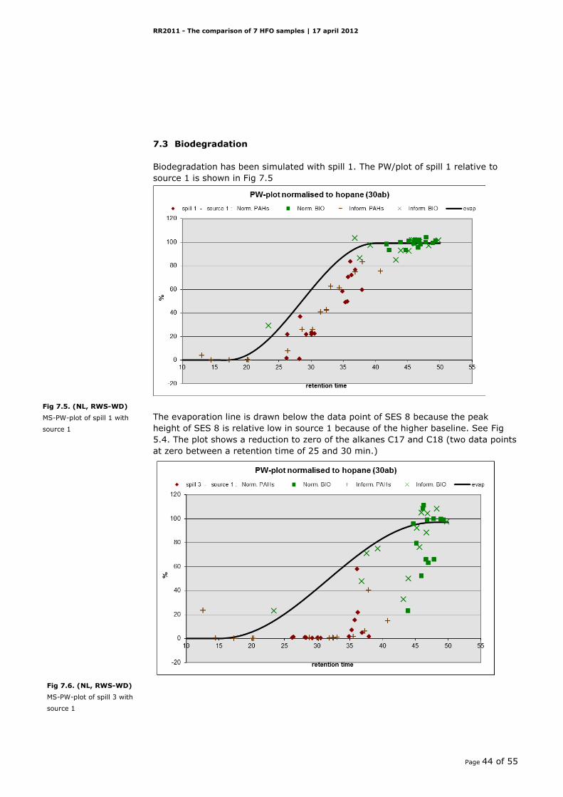
7.3 Biodegradation

Biodegradation has been simulated with spill 1. The PW/plot of spill 1 relative to

source 1 is shown in Fig 7.5

The evaporation line is drawn below the data point of SES 8 because the peak

height of SES 8 is relative low in source 1 because of the higher baseline. See Fig

5.4. The plot shows a reduction to zero of the alkanes C17 and C18 (two data points

at zero between a retention time of 25 and 30 min.)


MS-PW-plot of spill 1 with

source 1


MS-PW-plot of spill 3 with

source 1


Page 45 of 55

The PW/plot of spill 3 relative to source 1 is shown in Fig 7.6. The evaporation line

neglects the C1 decalins data point, is drawn again below the data point of SES 8

and uses the triterpanes C24 and C25 at 80% and the hopanes as references.

N.B. The data points of the C1-decalins and SES 8 are on the same level of about 23%. The

evaporation line of spreadsheet file v51 is designed to start always from zero. Spill sample 3 is

from a 10 years old patch of oil on a beach in between the vegetation. It is very well possible

that the lighter compounds in the upper layer of the patch are evaporated, but in a lower layer

still exist. For this PW-plot it would be useful to add the option to start the evaporation line at

a higher choosen level.

The plot shows not alone a reduction to zero for the alkanes C17 and C18, but also

for pristane, phytane and many PAH’s and some of the biomarkers.

The effects of biodegradation on the eight PAH ion chromatograms can be studied in

the loading plot of PC1. See Fig 7.7

- m/z 192 shows a reduction order of 2 M-phenantrene > 3M-P > 1M-P > 9/4 M-

P> 1 and 2 M-anthracene.

- m/z 202 reduction of fluoranthene and a better resistance of pyrene.

- m/z 206 evident changes in the C2-phenantrene isomers.

Fig 7.7 (IMOF)

PC1 loading plot of 8 PAH

ion chromatograms behind

each other. In red the

normal chromatogram. In

blue the relative differences

specific for biodegradation.


Page 46 of 55

- m/z 216 4 M-Py is the most resistant m/z 216 compound to “biodegradation”

followed by 1 M-Py and the other fluoranthene and benzofluorene isomers.

The same is the case for the C2-isomers (m/z 230)

- m/z 228 reduction of benz (a) anthracene

- m/z 242 evident changes in the C1 chrysene isomers.

- m/z 252 reduction of benzo (b) fluoranthene


Page 47 of 55

8 Judgement of the individual reports.

8.1 Evaluation methods

Gerhard and Paul have discussed how to judge the reports. Just reading them and

giving a final judgement in a description or figure is not sufficiently objective and

informative. So both of then made a proposal and optimized the method in

discussions.

8.2 Evaluation method of Gerhard

Gerhard has prepared Table 6.1 for report judgement:

Item Criteria 1 with 2

1 with 3

1 with 4

1 with 5

1 with 6

1 with 7

Sum

1 presence of means 2 2 2 2 2 2 12

2 oil type correct? 1 1 1 1 1 1 6

3 ratios correctly chosen/excluded 2 2 2 2 2 2 12

4 QM 2 2 2 2 2 2 12

5 interpretation of ratios and weathering

2 2 2 2 2 2 12

6 Right conclusion? 2 2 2 2 2 2 12

Max. reachable points 11 11 11 11 11 11 66

for every comparison

Item Criteria Comments

1 presence of means 0 or 2 Presence of all necessary means for tracing back a conclusion

2 oil type correct? 0 or 1

3 ratios correctly chosen/excluded 0 or 1 or 2

4 QM 0 or 1 or 2

Double measurements sd<5%, quality of chromatograms

5 interpretation of ratios and weathering

0 or 1 or 2

Explanations for differences >14%

6 Right conclusion? 0 or 2

0= not present/wrong/bad 1= fair 2= present/right/good

Table 6.1

Report evaluation by

Gerhard with regard to

correct and traceable

conclusions


Page 48 of 55

8.3 Evaluation method of Paul

Paul has prepared Table 6.2 for report judgement:

Item Main groups aspects points remarks

1 FID level 1.1 analysis analytical method and data quality

2 FID level 1.2 data evaluation which conclusions are drawn from the results, e.g. concentration

adjustment, oil type, elimination of samples.

3 MS level 2.1 analysis - visual inspection analytical method and data quality

4 MS level 2.2 PW-plots - ratios comp. integration, elimination of ratios, variance.

5 Result conclusions from chromatograms e.g. oil type, elimination of samples.

evaluation conclusions from PW-plots similarity and weathering aspects

conclusions from the ratio comparison similarity and weathering aspects.

6 Match conclusion

final match conclusions. Conclusions related to the scenario.

7 Reporting internal documentation results that are important for the final conclusions;

description of the reasons for conclusions.

8 Reporting external - summery report. Completeness according to CEN/Tr chapter 7.3

9 Overall Personal judgement of the whole report To be able to give an additional personal opinion.

impression Useful? I don't know We will see.

Total (ranks from 0 to 18 points) 0 For each item: 0 = bad 1 = fair 2 = good

Item 8 “External report” is for this year not used, because it was not requested in

the instructions. It should however be a part of the judgement of the next Round

Robins.

8.4 Judgement of the results

The individual reports of the participants are available for members of the

BonnOSInet expert group, but are treated as confidential for the public. Therefore it

does not make sense to discuss here the results of the judgement of the individual

reports even by using a code for each participant.

But certain aspects and the overall results can be shown and discussed. Therefore

they are reported in chapter 7 of the summary report while the results of the

judgement of the labs is shown in Table 6.3 (Identical to Table 3 of the executive

summary

Table 6.2

Report evaluation by Paul

with regard to correct and

traceable conclusions


Page 49 of 55

Lab code Method Paul Method Gerhard mean

Lab1 81 79 80

Lab2 100 100 100

Lab3 88 83 85

Lab4 100 100 100

Lab5 38 39 38

Lab6 56 52 54

Lab7 94 97 95

Lab8 100 100 100

Lab9 69 76 72

Lab10 88 82 85

Lab11 88 88 88

Lab12 75 82 78

Lab13 75 73 74

Lab14 81 74 78

Lab15 81 77 79

Lab16 81 88 85

Lab17 100 100 100

Lab18

Lab19 94 97 95

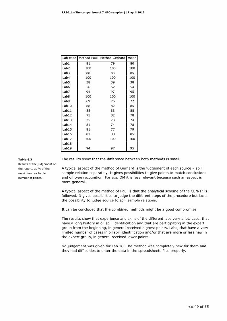
The results show that the difference between both methods is small.

A typical aspect of the method of Gerhard is the judgement of each source – spill

sample relation separately. It gives possibilities to give points to match conclusions

and oil type recognition. For e.g. QM it is less relevant because such an aspect is

more general.

A typical aspect of the method of Paul is that the analytical scheme of the CEN/Tr is

followed. It gives possibilities to judge the different steps of the procedure but lacks

the possibility to judge source to spill sample relations.

It can be concluded that the combined methods might be a good compromise.

The results show that experience and skills of the different labs vary a lot. Labs, that

have a long history in oil spill identification and that are participating in the expert

group from the beginning, in general received highest points. Labs, that have a very

limited number of cases in oil spill identification and/or that are more or less new in

the expert group, in general received lower points.

No judgement was given for Lab 18. The method was completely new for them and

they had difficulties to enter the data in the spreadsheets files properly.

Table 6.3

Results of the judgement of

the reports as % of the

maximum reachable

number of points.


Page 50 of 55


Page 51 of 55

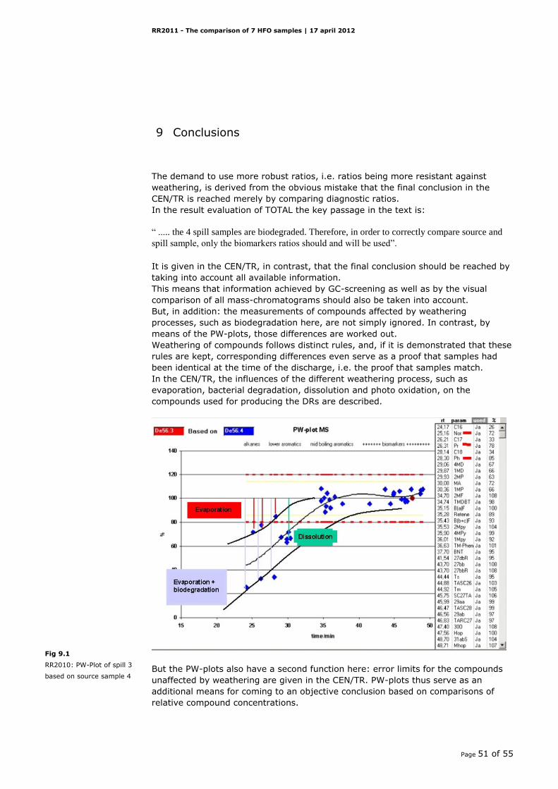
9 Conclusions

The demand to use more robust ratios, i.e. ratios being more resistant against

weathering, is derived from the obvious mistake that the final conclusion in the

CEN/TR is reached merely by comparing diagnostic ratios.

In the result evaluation of TOTAL the key passage in the text is:

“ ..... the 4 spill samples are biodegraded. Therefore, in order to correctly compare source and

spill sample, only the biomarkers ratios should and will be used”.

It is given in the CEN/TR, in contrast, that the final conclusion should be reached by

taking into account all available information.

This means that information achieved by GC-screening as well as by the visual

comparison of all mass-chromatograms should also be taken into account.

But, in addition: the measurements of compounds affected by weathering

processes, such as biodegradation here, are not simply ignored. In contrast, by

means of the PW-plots, those differences are worked out.

Weathering of compounds follows distinct rules, and, if it is demonstrated that these

rules are kept, corresponding differences even serve as a proof that samples had

been identical at the time of the discharge, i.e. the proof that samples match.

In the CEN/TR, the influences of the different weathering process, such as

evaporation, bacterial degradation, dissolution and photo oxidation, on the

compounds used for producing the DRs are described.

But the PW-plots also have a second function here: error limits for the compounds

unaffected by weathering are given in the CEN/TR. PW-plots thus serve as an

additional means for coming to an objective conclusion based on comparisons of

relative compound concentrations.

Fig 9.1

RR2010: PW-Plot of spill 3

based on source sample 4


Page 52 of 55

In summary: to reduce the role of the PW-plots to their mere function for deleting

diagnostic ratios, which are affected by weathering, must therefore be regarded as

an obvious mistake.

Admittedly, not all situations and circumstances are covered by the CEN/TR, and

nothing is said about the bacterial degradation of biomarkers, which are the most

stable compounds here. But the task to identify 10 year old oil samples must be

regarded as a very special one, which cannot be solved my means of only 3 or 4

samples, taken at the beginning and at the end of this time.

Nevertheless, the analyst is not left alone here: in RR2011 additional information is

present by comparing the two 10 year old samples among each other, and their

relation to the samples, which were taken one year after the accident.

Of course, it would be much better, if much more samples, taken also over the

years, were present. Thus, in this Round Robin, the participants got only a short

insight into the problems, which appear during post-spill investigations, conducted

over a longer time.

But PW-plots may also lead to additional “problems”: the PW-plots here show

differences, which are not found, when only the diagnostic ratios are compared: the

reduction of the triaromatic steranes. These compounds are found to be very stable

against biodegradation.

Spill 2 gives an answer here: as spill 2 is rarely affected by biodegradation,

biodegradation cannot be responsible for the reduction. The reduction must have

been caused by dissolution and photo oxidation. It could be found out that

especially photo oxidation led to strong reductions of other aromatics in this sample.

Fig 9.2

PW-Plots of spills 1 to 4,

which show the increasing

reduction of the lower

boiling (M-Phens, M-DBTs)

and mid boiling aromatics

(pyrenes) from spills 1and 2

over spill 4 to 3, the

reduction of the TAS in spills

2 to 4, and the stepwise

reduction of 27dbS+27dbR

and 27bb from spills 1 and

2 over spill 4 to spill 3.


Page 53 of 55

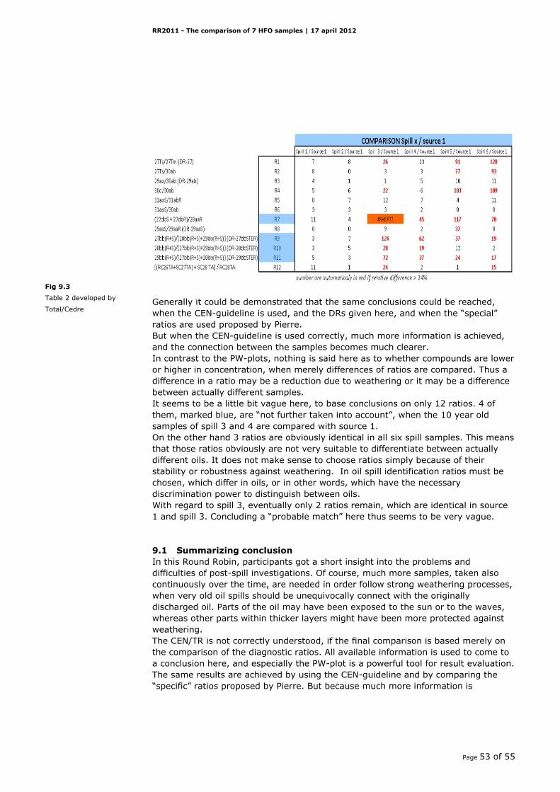
Generally it could be demonstrated that the same conclusions could be reached,

when the CEN-guideline is used, and the DRs given here, and when the “special”

ratios are used proposed by Pierre.

But when the CEN-guideline is used correctly, much more information is achieved,

and the connection between the samples becomes much clearer.

In contrast to the PW-plots, nothing is said here as to whether compounds are lower

or higher in concentration, when merely differences of ratios are compared. Thus a

difference in a ratio may be a reduction due to weathering or it may be a difference

between actually different samples.

It seems to be a little bit vague here, to base conclusions on only 12 ratios. 4 of

them, marked blue, are “not further taken into account”, when the 10 year old

samples of spill 3 and 4 are compared with source 1.

On the other hand 3 ratios are obviously identical in all six spill samples. This means

that those ratios obviously are not very suitable to differentiate between actually

different oils. It does not make sense to choose ratios simply because of their

stability or robustness against weathering. In oil spill identification ratios must be

chosen, which differ in oils, or in other words, which have the necessary

discrimination power to distinguish between oils.

With regard to spill 3, eventually only 2 ratios remain, which are identical in source

1 and spill 3. Concluding a “probable match” here thus seems to be very vague.

9.1 Summarizing conclusion

In this Round Robin, participants got a short insight into the problems and

difficulties of post-spill investigations. Of course, much more samples, taken also

continuously over the time, are needed in order follow strong weathering processes,

when very old oil spills should be unequivocally connect with the originally

discharged oil. Parts of the oil may have been exposed to the sun or to the waves,

whereas other parts within thicker layers might have been more protected against

weathering.

The CEN/TR is not correctly understood, if the final comparison is based merely on

the comparison of the diagnostic ratios. All available information is used to come to

a conclusion here, and especially the PW-plot is a powerful tool for result evaluation.

The same results are achieved by using the CEN-guideline and by comparing the

“specific” ratios proposed by Pierre. But because much more information is

Fig 9.3

Table 2 developed by

Total/Cedre


Page 54 of 55

achieved, when the CEN-guideline is used, conclusions achieved here are much

more substantiated.

There is definitely no need to change the diagnostic ratios as given in the CEN-

guideline


Page 55 of 55

10 References

[1] Currie, L.A., Svehla, G.. Nomenclature for the presentation of results of chemical

data. Pure & Appl. Chem. , Vol 66, No 3, pp 595-608, 1994.

[2] Miller, J.S. and Olejnic D., Photolysis of polycyclic aromatic hydrocarbons in

water. Wat. Res. Vol. 35, No 1, pp. 233-243, 2001.

[3] Christensen, J.H. and Tomasi, G. A multivariate approach to oil hydrocarbon

fingerprinting and spill source identification: in Z Wang & SA Stout (eds), Oil spill

environmental forensics: fingerprinting and source identification. Academic Press,

Incorporated, chapter 9, pp. 293-325, 2006.

Documents

RR2011 - The comparison of 7 HFO · PDF fileMUMM Oostende (BE) Marijke Neyts Petrobras Rio de Janeiro (BR) Fabiana D. C. Gallotta ... The accident occurred 200 miles off the coast