RSMGUI User Guide

Regional Simulation Model Graphical User Interface

RSMGUI Ver. 4.1.7 (64bit) Document Last Updated on April 14, 2009

South Florida Water Management District (SFWMD) Hydrologic & Environmental Systems Modeling Department (HESM)

3301 Gun Club Road, West Palm Beach, FL 33406

ii

Revision History for The Regional Simulation Model (RSM)

Graphical User Interface (GUI) User Guide

Version Name Date Comments 1.0 Rick Miessau 2/9/2007 Initial Version. 3.0.4 Rick Miessau 12/11/2007 Version 3.0.4 Release update 3.0.11 Rick Miessau 3/28/2008 Version 3.0.11 Release update 3.0.13 Rick Miessau 4/18/2008 Version 3.0.13 Release update 3.0.15 Rick Miessau 5/23/2008 Version 3.0.15 Release update 3.0.16 Rick Miessau 5/30/2008 Version 3.0.16 Release updates 3.0.17 Rick Miessau 6/20/2008 Final 32bit version of RSMGUI

3.0.17b 3.0.17b Rick Miessau 6/30/2008 Updated to reflect all tools in the final 32bit

version 4.0.0 Rick Miessau 6/30/2008 Version 4.0.0 64bit Release Update 4.1.0 Rick Miessau 12/15/2008 Version4.0.9 update.

New: cell comparison tool, Google Mesh Variable tool, Tecplot Loader, Parameter Sensitivity tool updated: transect tool, Estuary PMGs, Run Model, Scenario Builder, Watermover_CAT

4.1.4 Rick Miessau 2/4/2009 Version 4.1.3 update Updated cover, Google Earth Animation New: Vector QA, Parameter Sensitivity, Google Mesh Variable

4.1.5 Rick Miessau 3/26/2009 Version 4.1.5 update Updated: cover, Mesh Intersect New: Mesh Export, GIS transect tool, Chloride SQL to DSS tool

4.1.6 Rick Miessau 4/16/2009 Version 4.1.6 update Updated: watermover_CAT, Google Animation w/ hydrographs New: RSM WEB GUI, DBHYDRO SQL to DSS tool,

4.1.7 Rick Miessau Version 4.1.7 update Updated: waterbody_PLOT, CAT, watermover _PLOT, CAT

iii

List of Figures........................................................................................................................ vii List of Tables .......................................................................................................................... ix Preface...................................................................................................................................... x Introduction.............................................................................................................................. 1

1.1 RSM GUI Programming Information............................................................................ 1 1.2 Programming Dependencies on the Geodatabase...................................................... 1 1.3 How Are RSM Input Files Generated? ........................................................................ 2 1.4 How This Manual Should Be Used.............................................................................. 2

General Overview .................................................................................................................... 3 2.1 RSM GUI Vision Statement......................................................................................... 3 2.2 Some Important Things to Know ................................................................................. 3 2.3 RSM Basics................................................................................................................. 3

Getting Started in GIS and Accessing the RSM GIS Toolbar............................................... 7 3.1 Open RSM Template Geodatabase in ArcGIS Using Citrix......................................... 7 3.2 RSM GIS Major Elements ........................................................................................... 8 3.3 Accessing the RSM GIS Toolbar............................................................................... 12

Building an RSM Geodatabase............................................................................................. 13 4.1 Mesh Tools................................................................................................................ 13 4.2 Load Simple Mesh Tool............................................................................................. 13 4.3 Load SFRSM Template............................................................................................. 13 4.4 Export Mesh .............................................................................................................. 14 4.5 Intersect Mesh........................................................................................................... 14 4.5 Viewing Attributes.................................................................................................. 15 4.6 CHANGING ATTRIBUTES........................................................................................ 18 4.7 Enable and Disable Geodatabase Features.............................................................. 18 4.8 Segmenting Canals ................................................................................................... 19 4.9 Index Tool ................................................................................................................. 21

Generate XML Files ............................................................................................................... 22 5.1 Generating the MSE (Water Control Unit) XML’s ...................................................... 22 5.2 Lake Watermover XML.............................................................................................. 22 5.3 Watermover XML ...................................................................................................... 23 5.4 Levee Seepage XML................................................................................................. 23 5.5 Waterbody List .......................................................................................................... 23 5.6 PWS XML.................................................................................................................. 23 5.7 Junction Blocks ......................................................................................................... 23 5.8 Cell Monitors ............................................................................................................. 24 5.9 Transect Flowgage.................................................................................................... 24 5.10 Levee BC .................................................................................................................. 25 5.11 Waterbudget.............................................................................................................. 25 5.12 Headstage................................................................................................................. 25 5.13 Mesh Attribute ........................................................................................................... 25 5.14 Canal File (.MAP) ...................................................................................................... 25

Utilities.................................................................................................................................... 28 6.1 Compare Mesh.......................................................................................................... 28 6.2 Compare Framework................................................................................................. 29 6.3 Build NetCDF Rasters ............................................................................................... 29 6.4 Reporting Triggers..................................................................................................... 30

iv

6.5 Mesh Suitability Test ................................................................................................. 30 Browser Based GIS Tools..................................................................................................... 31

7.1 Arc GIS Server Usage and Capabilities .................................................................... 32 7.2 Uploading an RSM Geo-database............................................................................. 32 7.3 RSM GIS Server9.2 Main Navigation Buttons........................................................... 32 7.4 RSM GIS TOOL MENU............................................................................................. 33 U

7.5 Results Menu ............................................................................................................ 33 7.6 Map Contents Menu .................................................................................................. 34 7.7 Navigation ................................................................................................................. 34 7.8 Overview Menu ......................................................................................................... 35 7.9 RSM GUI Tools Menu ............................................................................................... 35 7.10 HSE Network Tools Menu ......................................................................................... 35 7.11 MSE Network Tools Menu......................................................................................... 36 7.12 Generate XML Tools Menu ....................................................................................... 37

The RSM GUI.......................................................................................................................... 38 8.1 Starting the RSM GUI................................................................................................ 38 8.2 File Menu .................................................................................................................. 39 8.3 Exit Feature............................................................................................................... 39

PreProcessing Menu ............................................................................................................. 40 9.1 Edit an XML File Tool ................................................................................................ 40 9.2 Scenario Builder Tool ................................................................................................ 40

9.2.1 Entity .................................................................................................................. 41 9.2.2 Control ............................................................................................................... 43 9.2.3 Conveyance Tool ............................................................................................... 44 9.2.4 Svconverter ........................................................................................................ 45 9.2.5 Transmissivity Tool ............................................................................................ 45 9.2.6 arcs (xsentry) ..................................................................................................... 47 9.2.7 MSE Controllers ................................................................................................. 47 9.2.8 BC Monitor ......................................................................................................... 48 9.2.9 Cell Monitor ........................................................................................................ 49 9.2.10 Flowgage............................................................................................................ 50 9.2.11 Global Monitor.................................................................................................... 51 9.2.12 Impoundment Monitor ........................................................................................ 51 9.2.13 Junction Monitor................................................................................................. 51 9.2.14 Segment Monitor................................................................................................ 51 9.2.15 Waterbudget Output........................................................................................... 52 9.2.16 WCD Monitor...................................................................................................... 52 9.2.17 WCU Monitor...................................................................................................... 52 9.2.18 WM Monitor........................................................................................................ 52

9.3 PWS XML Tool.......................................................................................................... 53 9.4 Rulecurve XML.......................................................................................................... 54 9.5 Reverse Engineer...................................................................................................... 54 9.6 Chloride SQL to DSS ................................................................................................ 55 9.6 DBHYDRO SQL to DSS............................................................................................ 55

Run Model Menu.................................................................................................................... 56 10.1 Run Model Tool ......................................................................................................... 56 10.3 Parameter Sensitivity Tool ........................................................................................ 57 10.2 View Model Log......................................................................................................... 60

View Model Results Menu..................................................................................................... 62

v

11.1 Results Viewer .......................................................................................................... 62 11.1.1 Pest Visualization............................................................................................... 64

11.2 ncBrowse .................................................................................................................. 66 11.3 HecDSSVue .............................................................................................................. 66 11.4 DSSMapVue.............................................................................................................. 67 11.5 OpenDX .................................................................................................................... 68 11.6 Cell Comparison Hydrographs .................................................................................. 70 11.7 Waterbody_CAT........................................................................................................ 72 11.8 Waterbody_PLOT...................................................................................................... 73 11.9 Watermover_CAT...................................................................................................... 74 11.10 Watermover_PLOT................................................................................................ 76 11.11 Google KMZ Animation.......................................................................................... 77 11.12 Transect Tool......................................................................................................... 81

Process Model Output Menu ................................................................................................ 83 12.1 Waterbudget Residual Animation .............................................................................. 83 12.2 NCDump ................................................................................................................... 85 12.3 List of Mesh Cells ...................................................................................................... 85 12.4 WBBUD..................................................................................................................... 86 12.5 NC Difference Tool.................................................................................................... 88 12.6 Dynamic Charting Tool.............................................................................................. 89 12.7 EFDC Structure Translator ........................................................................................ 92 12. 8 EFDC Headstage Translator.................................................................................. 93 12.9 Tecplot Loader .......................................................................................................... 93

Output Graphics Menu.......................................................................................................... 94 13.1 DSS Stage/Flow Plots ............................................................................................... 95 13.2 NetCDF Stage/Flow Plots ......................................................................................... 96 13.3 Canal Animation Graphics......................................................................................... 98 13.4 Presentation Graphics............................................................................................... 99 13.5 Verification Plots...................................................................................................... 102 13.6 Inundation Report.................................................................................................... 103 13.7 Levee Seepage Report ........................................................................................... 105

Performance Measure Graphics......................................................................................... 108 14.1 LOK PMG’s ............................................................................................................. 109

14.1.1 LOK Envelope PMG........................................................................................ 109 14.1.2 LOK Minimum Water Level ............................................................................. 112

14.2 Estuary PMG’s ........................................................................................................ 113 14.2.1 Caloo and STL ................................................................................................ 113 14.2.2 Caloo and STL (NERSM rivers) ...................................................................... 116 14.2.3 C43 Target Flow Index.................................................................................... 119

14.3 KISS PMG’s ............................................................................................................ 120 14.3.1 LKB Mean Monthly Flows................................................................................ 120 14.3.2 LKB Seasonal Min/Max Flows......................................................................... 121 14.3.3 LKB 14 Day Low Flows ................................................................................... 123 14.3.4 KUB Probable High Lake Stages .................................................................... 125

14.4 PMI’s ....................................................................................................................... 128 14.4.1 LOK Stage Duration Curve.............................................................................. 128 14.4.2 Water Supply Indicator 7 Worst Years ............................................................ 129 14.4.3 4-1in-1 LOK Water Supply Indicator................................................................ 130 14.4.4 Intra-Annual Lake Variability ........................................................................... 131

vi

14.4.5 KUB Stage Duration for Navigation................................................................. 132 Cluster Tools Menu ............................................................................................................. 134

15.1 Top Processes ........................................................................................................ 134 15.2 Load ........................................................................................................................ 134 15.3 Cluster Report ......................................................................................................... 135

HELP Menu........................................................................................................................... 136 16.1 About… ................................................................................................................... 136 16.2 Request Help........................................................................................................... 136 16.3 RSM Homepage...................................................................................................... 136 16.4 RSM GUI UserGuide............................................................................................... 137 16.5 SFRSM Toolbar Python Documentation ................................................................. 138 16.6 CVS/SVN Code Repository..................................................................................... 138 16.7 Bugzilla 2.22............................................................................................................ 139 16.8 fixDSS ..................................................................................................................... 139 16.9 Customize Toolbar .................................................................................................. 139

Appendix A - Definitions, Abbreviations and Acronyms ................................................. 140 Appendix B – RSM Template Geodatabase Report .......................................................... 142 Appendix C – Preparing an RSM Scenario........................................................................ 158 Appendix D - RSM Input Files............................................................................................. 159 Appendix E – The Calibration XML .................................................................................... 162 Appendix F – The PMG SOURCE FILE............................................................................... 173 Appendix G – The LeveeSeepage Report Input Files....................................................... 175

List of Figures Figure 1: RSM GUI GIS Workflow Diagram............................................................................... 5 Figure 2: RSM Process Flow Diagram....................................................................................... 6 Figure 3: View of the c-111_12_5a.mdb geodatabase .............................................................. 8 Figure 4: Using the GIS Identify Tool....................................................................................... 10 Figure 5: Viewing GIS Attributes.............................................................................................. 11 Figure 6: View of RSM GIS Toolbar ........................................................................................ 12 Figure 7: Generate Mesh Attributes Tool................................................................................. 15 Figure 8: GIS Map Showing the Active Layers and Anchored RSM Toolbar ........................... 16 Figure 9: View of Selected Structure Highlighted in Blue and Attribute Information ................ 17 Figure 10: Enabled Attribute Field ........................................................................................... 18 Figure 11: Reach 617 Before Segmenting............................................................................... 19 Figure 12: Segmentation Tool ................................................................................................. 20 Figure 13: Reach 617 After Segmentation............................................................................... 20 Figure 14: Canal .MAP Tool (default view) .............................................................................. 26 Figure 15: Canal .MAP Tool (advanced Options View) ........................................................... 27 Figure 16: Compare Mesh Tool ............................................................................................... 28 Figure 17: Compare Framework Tool ...................................................................................... 29 Figure 18: Build NetCDF Rasters Tool .................................................................................... 29 Figure 19: Reporting Triggers Tool.......................................................................................... 30 Figure 20: Mesh Suitability Tool .............................................................................................. 30 Figure 21: ArcGIS Server 9.2 Application Displaying the C-111 Geodatabase ....................... 31 Figure 22: The RSM GUI Python Toolbar................................................................................ 38 Figure 23: The RSM GUI File Menu ........................................................................................ 39

vii

Figure 24: The PreProcessing Menu ....................................................................................... 40 Figure 25: Scenario Builder Tool ............................................................................................. 41 Figure 26: PWS XML Tool and PWS XML file ......................................................................... 53 Figure 27: Rule Curve Tool...................................................................................................... 54 Figure 28: Reverse Engineer Tool........................................................................................... 54 Figure 29: The Run Model Menu ............................................................................................. 56 Figure 30: Run Model Tool ...................................................................................................... 56 Figure 31: Output from Parameter Sensitivity Tool.................................................................. 59 Figure 32: Interface Used to Search the Model Log ................................................................ 60 Figure 33: Sample Output from the Run Model Log ................................................................ 61 Figure 34: The View Model Results Menu............................................................................... 62 Figure 35: ResultsViewer start-up interface............................................................................. 62 Figure 36: Results Viewer Display Windows ........................................................................... 63 Figure 37: Pest Visualization Options Menu............................................................................ 64 Figure 38: Viewing Jacobian Matrix Output from PEST........................................................... 65 Figure 39: Viewing Correlation Matrix Output from PEST........................................................ 65 Figure 40: ncBrowse Tool........................................................................................................ 66 Figure 41: Hec-DSSVue Tool .................................................................................................. 67 Figure 42: Hec-DSS MapVue Tool .......................................................................................... 67 Figure 43: Open_DX Graphic Window .................................................................................... 69 Figure 44: Open_DX Animation Output ................................................................................... 70 Figure 45: Cell Comparison Hydrograph Tool ......................................................................... 72 Figure 46: Waterbody_CAT Tool ............................................................................................. 73 Figure 47: Waterbody_PLOT Tool........................................................................................... 74 Figure 48: Output from the Watermover_CAT Tool ................................................................. 76 Figure 49: Watermover_PLOT Tool......................................................................................... 77 Figure 50: Google Earth Tool .................................................................................................. 79 Figure 51: GoogleEarth KMZ Animation Showing ComputedHead Elevations in 2D .............. 80 Figure 52: Output from the RSM GUI Transect Tool ............................................................... 82 Figure 53: Process Model Output Menu .................................................................................. 83 Figure 54: Waterbudget Residual Animation Input Options ..................................................... 84 Figure 55: Output from the Waterbudget Residual Animation Tool ......................................... 85 Figure 56: Output from List of Mesh Cells Tool ....................................................................... 86 Figure 57: WBBUD Main Options Menu .................................................................................. 87 Figure 58: Output report from WBBUD for waterbody 19 ........................................................ 88 Figure 59: NC Difference Tool Menu ....................................................................................... 88 Figure 60: Dynamic Charting Tool Initial menu........................................................................ 89 Figure 61: Dynamic Charting main settings menu ................................................................... 90 Figure 62: Dynamic Charting sample output............................................................................ 91 Figure 63: Dynamic Charting settings file ................................................................................ 92 Figure 64: Output Graphics Menu ........................................................................................... 94 Figure 65: DSS Stage/Flow Plots Input Menu ......................................................................... 95 Figure 66: Output from DSS Stage/Flow Plot Tool .................................................................. 95 Figure 67: output from the netCDF Stage/Flow Tool ............................................................... 97 Figure 68: Canal Animation Graphics Menu ............................................................................ 98 Figure 69: Output from the Canal Animation Graphics Tool .................................................... 99 Figure 70: Presentation Graphics Tool Menu ........................................................................ 100 Figure 71: Output from the Presentation Graphics Tool ........................................................ 101 Figure 72: Output from the Verification Tool .......................................................................... 103

viii

Figure 73: Inundation Report Tool Options Menu.................................................................. 104 Figure 74: Output from the Inundation Report Tool ............................................................... 105 Figure 75: Levee Seepage Report Options Menu ................................................................. 106 Figure 76: Output from the Levee Seepage Report Tool ....................................................... 107 Figure 77: Performance Measure Graphics Menu................................................................. 108 Figure 78: lo1_weekly_low_lake_annualized.pdf................................................................... 109 Figure 79: lo2_weekly_high_lake_annualized.pdf ................................................................. 110 Figure 80: lo3_weekly_low_annualized.pdf ........................................................................... 110 Figure 81: lo3_weekly_high_lake_annualized.pdf ................................................................. 111 Figure 82: lok_minlvl_bar.pdf................................................................................................. 112 Figure 83: caloos_2800_4500_flow_bar.pdf.......................................................................... 113 Figure 84: caloos_salinity_flow_bar.pdf................................................................................. 114 Figure 85: stluc_2000_flow_bar.pdf....................................................................................... 114 Figure 86: stluc_salinity_flow_bar.pdf.................................................................................... 115 Figure 87: caloos_nersm_2800_4500_flow_bar.pdf.............................................................. 116 Figure 88: caloos_nersm_salinity_flow_bar.pdf..................................................................... 117 Figure 89: stluc_nersm_2000_flow_bar.pdf........................................................................... 117 Figure 90: stluc_nersm_salinity_flow_bar.pdf........................................................................ 118 Figure 91: C43 Target Flow Index PMG ................................................................................ 119 Figure 92: kiss-pmg1.pdf LKB Mean Monthly Flows.............................................................. 120 Figure 93: kiss-pmg2.pdf maximum monthly flows at S-65.................................................... 121 Figure 94: kiss-pmg2.pdf minimum monthly flows at S-65..................................................... 121 Figure 95: kiss-pmg2.pdf maximum monthly flows at S-65E ................................................. 122 Figure 96: kiss-pmg2.pdf minimum monthly flow at S-65E.................................................... 122 Figure 97: kiss-pmg3.pdf Flows at S-65 ................................................................................ 123 Figure 98: kiss-pmg3.pdf Flows at S-65E.............................................................................. 124 Figure 99: kiss-pmg4.pdf ....................................................................................................... 125 Figure 100: kiss-pmg4.html ................................................................................................... 127 Figure 101: pmi1.pdf.............................................................................................................. 128 Figure 102: losa_cutback_yrs_bar.pdf................................................................................... 129 Figure 103: losa_dmd_4in1.pdf ............................................................................................. 130 Figure 104: pmi8.html ............................................................................................................ 131 Figure 105: pmi9.pdf.............................................................................................................. 132 Figure 106: Cluster Tools Menu ............................................................................................ 134 Figure 107: Display produced by the "Top" Command.......................................................... 134 Figure 108: Display produced by the "Load" Command ........................................................ 134 Figure 109: Help Menu .......................................................................................................... 136 Figure 110: RSM Homepage ................................................................................................. 137 Figure 111: RSM GUI Customized Toolbar ........................................................................... 139

List of Tables Table 1: Sample RSM Geodatabase Summary Report ........................................................... 10

ix

Preface This document is a guide to using the Regional Simulation Model (RSM) Graphical User Interface (GUI). The RSM GUI is a collection of tools and data methods organized under a common toolbar to aid and simplify preparing and analyzing an RSM model run. A geographic information system (GIS) has been utilized to capture and organize the data representing the physical features in the model such as; the mesh, canals, structures and complex interconnectivity of the features in the hydrologic system. At the time of this writing, the RSM GUI helps automate approximately 90% of the input files and provides 66 post-processing features. Version 4.0.0 is the first 64bit version of the RSM GUI. Users on a 32bit computer can run the rsmgui32 command to access an older version of the RSM GUI that is unsupported, but should run on a 32bit computer. Acknowledgements The South Florida Water Management District gratefully acknowledges the contributions of the professionals who have made this project a reality. The RSM Graphical User Interface has been evolving over several years and many people have contributed to this development effort.

Project Manager: Rick Miessau, Project Manager has organized and led this effort while trying to keep pace with the evolving state of the RSM and changing needs of the RSM model implementers. While diligently sticking to a requirements driven approach the GUI development has been carried out following a rapid or extreme programming methodology.

Principal Engineers: Michael “Clay” Brown, Sr. Hydrologic Modeler and Dr. Eric Flaig PhD,

Sr. Engineer and Dr. Ruben Arteaga, Lead Hydrologic Modeler were the principal engineers from whom the high level requirements were gathered. Clay has provided the GUI development team with a combined perspective of both an implementer of the RSM, a developer of GIS and a GUI application developer. Eric has provided training support, engineering insight and quality assurances throughout the life of this effort.

Development Team: The RSM GUI has been designed and developed by Aimond Alexis, Joseph

Rodrigues, Mike Warner, Charles Haynes and Bruce Hammond (contractor) and incorporates contributions from other very talented programmers. Vic Kelson is especially recognized for contributing the design and XML interface for the original RSM GUI.

FOR FURTHER INFORMATION CONTACT:

Rick Miessau, PMP Sr. Project Manager Hydrologic and Environmental Systems Modeling Department, 4510 South Florida Water Management District 3301 Gun Club Road, West Palm Beach, FL 33406 561-682-6521 rmiessau@sfwmd.gov

x

Chapter 1

Introduction The Regional Simulation Model (RSM) is a regional hydrologic model developed principally for application in South Florida. The RSM simulates the coupled movement and distribution of groundwater and surface water throughout the model domain using a Hydrologic Simulation Engine (HSE) to simulate the natural hydrology and a Management Simulation Engine (MSE) to provide a wide-range of operational capability. The RSM has been developed on a sound conceptual and mathematical framework that allows it to be applied generically to a wide range of hydrologic situations. The RSM HSE Users Manual should be consulted for the guiding principals and engineering specifics on how an RSM model should be set up to properly model hydrologic alternatives. This RSM GUI User Manual has been written as a companion to the RSM HSE User Manual. New users of the RSM should attend the RSM Training class after which this manual will offer practical assistance and step-by-step instructions on how to pre- and post-process an implementation of the RSM.

1.1 RSM GUI Programming Information The RSM GUI has been written using the Python programming language. The RSM GIS Toolbar, which a collection of pre-processing tools has been written in C-sharp (C#) and runs inside of ESRI’s ArcGIS 9.2. As the RSM continues to evolve and take on new the RSM GUI will also evolve to meet the changing needs of the modelers. As of March 2009, the RSM GIS Toolbar contains 37 pre-processing functions. The RSM GUI contains 67 features to run and post-process RSM data. All sample data referenced within this manual can be found on the whqoom01d server in:

/opt/local/share3/share/samples/

1.2 Programming Dependencies on the Geodatabase Early on in the design phase of the RSM GUI an ESRI ArcGIS personal geodatabase was chosen to be the primary repository for all spatial data. This geodatabase contains descriptions and attributes pertaining to all physical features being simulated by an RSM run. Once the attributes in the geodatabase have been setup to represent the desired conditions to be modeled, the GUI tools read the geodatabase and automate assembly of the RSM input files. Work is under way to migrate the RSM personal geodatabase to an Arc SDE versioned database. The data elements stored in the RSM geodatabase were selected based on the needs of the modelers and the prescribed content of the model input files. The geodatbase schema was designed to facilitate development of applications to automatically generate the RSM files. While the database schema must be adhered to for the RSM GUI tools to work, the schema can also be expanded to fit each modelers specific application of the RSM. A guiding principle of implementing a standard data schema and offering flexible user options has strongly influenced the GUI development. The RSM geodatabase schema can be reviewed via the published geodatabase report in Appendix A.

1

1.3 How Are RSM Input Files Generated? Input files for the RSM can be created a number of different ways: by-hand, by running custom scripts, by the RSM GIS tools or copied from other users. The recommended method for creating RSM input files is to assemble a geodatabase based on the RSM schema and generate the files using the RSM GIS tools. This ensures consistency of formatting and the use of documented methods. The resulting files can be verified and are self-documenting using contents in the geodatabase used to create the files. Once the modeler is satisfied with the data parameters the GUI has been designed to function very efficiently against the data schema and offer a fully automated process to generate the files needed to assemble an RSM run. Several of the tools are single click applications, yet they perform full geo-processing and generate files base on geospatial relationships within the geodatabase. By generating all RSM input files from a geodatabase the files themselves become expendable and can always be easily re-generated from the database using the GUI. The RSM GIS tools provide self-documenting header information to help identify the geodatabase from which the resulting files were generated.

1.4 How This Manual Should Be Used This RSM GUI Manual does not make any attempt to guide or explain engineering principles behind setting up a model run; rather it covers the steps taken by a modeler while setting up a simulation only after the conditions to be reflected in the model have been chosen. The template geodatabase has been designed to contain sufficient information to represent the range of conditions and interactions expected to be included in the south Florida hydrologic network. Following the steps in this manual should help guide a modeler in setting up their own RSM run using their own data. Given the flexibility in the RSM and the broad-range of ways to configure a run we tried to choose the best examples offering some of the most common ways the model is being used at the time of writing this manual. By following the examples in this manual, modelers should gain a basic understanding of how to assemble RSM input files using the RSM GUI. Figure 1 is a workflow diagram showing how the data is assembled in the geodatabase during the setup of a typical RSM simulation. SYMBOLS

Indicates steps taken to perform a specific task and should be tried by the reader of this manual

Indicates a valuable tip containing specific requirements, conditions or assumptions

Indicates features only available to users on the SFWMD network

The example C-

s used in this manual are intended to provide a step-by-step example on how to use each tool in the RSM GUI. The examples chosen are based on the RSM benchmarks and an implemented111 basin run. All sample data used in these examples are available on the server where the RSM GUI is being run or they can be found on the RSM DVD.

Sample GIS Data Location: /opt/local/share3/share/samples/

2

Chapter 2

General Overview

2.1 RSM GUI Vision Statement The vision statement for the RSM GUI is to deliver a graphical interface that will help make the RSM the most admired and widely used hydrologic model. The RSM GUI will be a comprehensive, easy-to-use modeling interface that will deliver output from the RSM in support of the DISTRICT’s scientific, engineering and decision making processes.

2.2 Some Important Things to Know There are some tips to keep in mind when building an RSM implementation. Understanding some of these important details and concepts will hopefully help modelers avoid making costly and time consuming mistakes. Tip 1: Every new RSM implementation should have an accompanying RSM compliant geodatabase that organizes the mesh, and physical features being represented in the model. Tip 2: When it is necessary to make changes to RSM input files, the changes should be applied to the geodatabase and then the RSM input files should be regenerated using the RSM GIS Tools. Tip 3: The RSM geodatabase can be added to but DO NOT remove any of the attributes that are part of the original template geodatabase. If the required features in the geodatabase are deleted or changed the RSM GIS pre-processing tools will not function correctly. Tip 4: The RSM GIS Toolbar is primarily maintained to run in GIS 9.2 on the SFWMD Citrix server. Tip 5: To run the RSM GUI from your Linux workspace, your environment setup files should contain the latest updates which can be found in: /opt/local/share3/bin/ .cshrc, .login, .bashrc, .bash_profile

2.3 RSM Basics To help orient new users, the following describes, in an overly simplified manner, the basic steps to building an implementation of the RSM. Step 1: Build a Mesh Currently GMS is the preferred method for building an RSM mesh. The mesh should be exported from GMS as a .2dm file. Steps 2-7 assume you have access to an ESRI ArcGIS9.2 environment.

3

Step 2: Build RSM Geodatabase Using ArcGIS9.2, open the RSM GIS Toolbar and select the Mesh Import tool. Import the .2dm file from GMS and combine it with the RSM Template Geodatabase. The resulting new geodatabase will use the .2dm mesh file to cookie-cut data layers from the template geodatabase. Step 3: Intersect Mesh with Desired attributes Open the RSM GIS Toolbar and select the Mesh Intersect Tool. This tool provides a method to populate the mesh with attributes such as soil_type, landuse_type, topo_elevation, etc. Step 4: Assign Canal Attributes Use the basic GIS functionality to select and assign attributes to the canal network such as width, slope, bottom_elevation, mannings_coefficient, etc. Step 5: Assign Structure Attributes Use the basic GIS functionality to select and assign attributes to the structures such as length, diameter, discharge_coefficient, etc. Step 6: Assign Levee and Boundary Conditions Use the basic GIS functionality to select and assign attributes to the mesh_framework layer to define boundary conditions and levees. Assign a levee type or boundary type and set the condition to enabled. Step 7: Generate the RSM Input Files Open the RSM GIS Toolbar and select the Generate XML Menu. These tools provide a method to easily generate RSM compliant XML files from information in the geodatabase. The remaining steps assume you are working from a Linux workspace. Step 8: Gather Standard Input Files Several input files are “standard” for all RSM implementations. These files should be gathered from appropriate sources: ETp_recomputed_tin.bin, Rain_v2.0-global.bin, mannings_prop.xml, evap_prop.xml, DSS input files, etc. Step 9: Setup Model Run Setup a directory for your model based on a previous run. Sub-folders such as: input, run_template and workspace should be created. Copy your newly created input files into the appropriate locations. Step 10: Create the Run XML Copy an existing run.xml to use as a template. Open the RSM GUI and select the Scenario Builder Tool from under the PreProcessing Menu which will help build XML blocks that can be copied into your run.xml. Start simple and add complexity. Make sure path references are correct. Step 11: Run the RSM Run your model. Make sure you are using a current version of the HSE and DTD files. Step 12: View Your RSM Output Open the RSM GUI and select from the variety of post-processing tools under the View Model Results Menu, the Process Model Output Menu, or the Output Graphics Menu.

4

Figure 1: RSM GUI GIS Workflow Diagram.

5

Figure 2: RSM Process Flow Diagram

6

Chapter 3

Getting Started in GIS and Accessing the RSM GIS Toolbar This chapter describes the pre-processing steps and usage of the tools in the RSM Geographic Information System Toolbar (RSM GIS TOOLBAR) to generate the input files needed to execute the Regional Simulation Model. The first step in preparing an RSM model is to start ArcGIS and assemble the spatial data into an RSM compliant personal geodatabase schema. The RSM GIS TOOLBAR can be accessed via the SFWMD Citrix GIS environment. If you are a new GIS user it would benefit you to attend SFWMD GIS I and II training classes. Ideally, modelers will also have attended the GIS for RSM Overview Training Class which helps orient new GIS users to the specific terminology and data elements used as part of RSM. This chapter will cover getting started in Citrix, accessing the RSM Toolbar and some of the fundamental RSM GIS terminology.

The RSM GIS Toolbar can also be installed locally for users running on a local copy of Arc GIS 9.2. Contact a member of the RSM GUI Development team to request help installing the RSM GIS Toolbar on your local PC.

3.1 Open RSM Template Geodatabase in ArcGIS Using Citrix An ArcGIS template geodatabase with a geometric network is used to store the RSM geographic data representing the mesh, canal network, watermovers and boundary conditions. Associated tables within the geodatabase contain information describing all features and attributes and can be queried to view conditions that will be represented in the RSM. You must have your own copy of the personal geodatabase to allow write access to the data.

Copy the sample RSM Geodatabase from this location: \\opt\local\share3\share\samples\gis\c-111_12_5a.mdb and copy it to a location where Citrix can access it such as your local harddrive.

Start Citrix on the SFWMD network

From the users desktop locate and open the icon called Citrix Program Neighborhood.

Open the folder named ArcGIS v9 Open the folder named ArcInfo Open double-click the icon named ArcMap-ArcInfo When ArcGIS opens, select “A New Empty map” and click OK. When the new map opens, right-click on Layers, under the Sthe right side of the window and select Add Data.

ource tab, on

Navigate to your copy of c-111_12_5a.mdb. Select the icon at the top of the window to “Connect to Folder”. Select C$ on ‘Client’ (V:) Find and double click the geodatabase on your local drive.

Select all features in the geodatabase by left-clicking on the first feature, hold down the shift button on your keyboard and then left-click the last feature in the list. Then click add.

7

After the map has drawn, zoom to the mesh by right-clicking on the layer named “mesh” and selecting “Zoom to Layer”.

Finally uncheck the boxes next to the layers named: sfrsm_gis_Net_Junctions, mesh_node, mesh_pnt, sfrsm_gis_Net2_Junctions, and watersheds.

Your personal copy of the Master RSM Geodatabase contains the RSM scheme and all the base attribute information and hydrologic network necessary for the RSM. The database schema within the geodatabase is required in order to use the custom RSM GIS tools. Explore the attribute tables and view the relational tables.

Figure 3: View of the c-111_12_5a.mdb geodatabase

3.2 RSM GIS Major Elements The geodatabase (mesh_import_template.mdb) provides a chance to explore the data schema and view the data objects expected to be present in a typical RSM model. The geodatabase has been designed to include class objects, relationship classes, domains, geometric network and attribute field names to help organize and contain the information needed to assemble RSM input files and to also support the development of the RSM GIS customized tools. A complete RSM Geodatabase Report is included in Appendix F.

8

GEODATABASE SUMMARY REPORT Object Name Object Type Geometry Subtypes canal_has_mse_unit RelationshipClass Canal->mse_unit canal Complex Edge Polyline canal

water mover mesh_bnd Simple Feature Polyline none mesh_framework Simple Edge Polyline none mesh_node Simple Junction Point none mesh_pnt Simple Feature Point none mesh Simple Feature Polygon none sfrsm_gis_net_junctions Simple Junction Point none sfrsm_Net Geometric Network sfrsm_gis_Net2_junctions Simple Junction Point none Sfrsm_gis_Net2 Geometric Network structure_has_culvert_box RelationshipClass structure->culvert_box none structure_has_culvert_circular RelationshipClass structure->culvert_circular structure_has_fixed_weir RelationshipClass structure->fixed_weir structure_has_mes_unit RelationshipClass structure->mse_unit structure_has_pump RelationshipClass structure->pump structure_has_spillway RelationshipClass structure->spillway structure_has_variable_weir RelationshipClass structure->variable_weir structure Simple Junction Point Diversion Structure

Inline Structure Junction Block

watersheds Simple Feature Polygon None culvert_box Table none None culvert_circular Table none None fixed_weir Table none None genstruc Table none None mse_const Table none None mse_dss Table none None mse_inout Table none None mse_node Table none None mse_rc Table none None mse_unit Table none None pump Table none None

9

spillway Table none None variable_weir Table none None boundary Domain Coded Value EnabledDomain Domain Coded Value rc_domain Domain Range vaule Domain Coded Value WM_type Domain Coded Value Table 1: Sample RSM Geodatabase Summary Report

Use the GIS Identify Tool to select and view features on the screen. Click on any cell in the mesh and view the attributes.

Figure 4: Using the GIS Identify Tool

10

Structure Structures include pumps, culverts, weirs, and spillways. Each structure can be associated with collection of units and each unit will be defined by attributes. Units such as culverts will have attributes such as: discharge_coefficient, culvert_length, name, manning_coefficient, width, height, diameter, etc. Mesh The Mesh is a layer of irregular triangle cells designed to capture the desired level of detail in areas of interest. Mesh cells may contain observation wells, structures, monitoring points. Mesh walls will typically follow geographic boundaries, levees, canals or other features that make up the framework of the region being modeled. Use the GIS identify tool and select inside a mesh cell. A typical mesh will be intersected with several other layers so that each mesh cell will contain a variety of attributes such as: bottom elevation, topo, conductivity, and landuse. Canal The Canal layer contains all the canal segments in the canal network. Segments are combined to make a canal reach which will span between two junctions. Canals can be made from multiple reaches which in turn can be made up from multiple segments. Each segment is defined by attributes such as: type, depth, slope, bottom_elevation, mannings_coefficient, name, upstream_structure, downstream_structure, etc.

Figure 5: Viewing GIS Attributes

11

3.3 Accessing the RSM GIS Toolbar The RSM GIS Toolbar has been created by the RSM GUI Development Team to help organize a collection of custom GIS applications that help assemble the data and generate files needed by the RSM. Built in ESRI ArcGIS geoprocessing capabilities and custom ArcObjects programming have been leveraged to meet the needs of modelers using the RSM. The RSM GIS Toolbar is a custom toolbar which can be activated by the user and will remain present as part of the user settings every time the user starts GIS until it is removed by the user. To access the RSM Toolbar for the first time, users must:

select the TOOLS Menu from the top of the GIS window select the CUSTOMIZE… option from the menu make sure the TOOLBAR tab has been selected check the box next to the RSM Toolbar Ver. 4.3

The RSM GIS Toolbar will appear as a new toolbar free floating on the screen. It can be anchored at the top of the GIS window along with the other standard GIS tools. Being a free floating toolbar it may be hidden behind your other windows.

Click on the menu button labeled “RSM GIS Toolset v4.3” to view the RSM GIS Toolbar.

It can be dragged around and positioned anywhere on the windows desktop. It may fall behind other windows open on the desktop. If this happens you can click on the toolbar on the lower system tray and it will call the most recent item to the foreground by clicking on it.

Figure 6: View of RSM GIS Toolbar

If RSM GIS Toolbar is sometimes hidden behind another CITRIX window, click on the CITRIX tab on the windows application tray and select the RSM GIS Toolbar ver. 4.3 to bring it to the foreground.

The toolbar contains a collection of tools to help manipulate the geodatabase and generate a variety of RSM input files. There are dropdown menus containing tools to help import the mesh, assemble the HSE Network, Generate the XMLs and Help. There are also place holders for future tools such as the MSE Network and to help create HPMs.

12

Chapter 4

Building an RSM Geodatabase A new RSM compliant Geodatabase can be created by adding a newly created mesh to the Master Development Geodatabase. The Master Development Geodatabase contains all the regional layers used by the RSM in the standard RSM database schema. The geodatabase layers can be clipped using any mesh to create a new project specific RSM compliant geodatabase suitable for setting up an RSM scenario. Other GIS layers can also be added from a variety of locations. Canal layers and structure layers must comply with the RSM database schema and participate in the RSM hydrologic network to properly function with the RSM GIS tools. Other layers can be added to aid in locating features and analyzing geographic conditions before the scenario is created.

4.1 Mesh Tools The first set of tools in the RSM GIS Toolbar are the Mesh Tools which assist with importing an irregular triangular mesh (.2dm file) from GMS and populating the mesh with data attributes. To view how these tools work we will start with a blank map and import a GMS mesh. There are two options for importing a mesh: Load SFRSM Template or Load Simple Mesh Tool.

4.2 Load Simple Mesh Tool The Load Simple Mesh tool takes input from the user and imports a GMS .2dm file resulting in a simple GIS mesh. This is a simplified approach to creating a new mesh in GIS.

Import a Simple Mesh

Select the Import Simple Mesh tool from the Mesh pulldown menu on the RSM GIS TOOLBAR.

Browse to the desired .2DM file you wish to import.

Browse to a location and input the name for a new geodatabase you wish to create.

Click Run A new geodatabase will be created which will contain three layers to define your new mesh.

4.3 Load SFRSM Template The Load SFRSM Template tool takes input from the user and combines a GMS mesh with a template geodatabase.

13

This results in a (cookie cut) RSM geodatsabase containing the base data layers and a new mesh. Select the Import SFRSM Template tool from the Mesh pulldown menu on the RSM GIS TOOLBAR.

Browse to the default geodatabase template or specify your own custom geodatabase

Browse to the desired .2DM file Browse to the corresponding .SHP file used to create the GMS framework Browse to a writable location and input the name for a new geodatabase you wish to create.

Click Run

4.4 Export Mesh The Export Mesh tool generates a new GMS .2DM file from a mesh layer that was modified using GIS. The tool requires the user specify the mesh layer and the output location for the new .2DM file.

4.5 Intersect Mesh After generating a new mesh the next step is to populate the mesh with attributes. The Generate Mesh Attribute tool automates intersecting the mesh with existing data layers from which the mesh will inherit new attributes.

Browse to the location of the target geodatabase containing the mesh and select the mesh-poly layer which will receive the new attributes.

Browse to the location of a geodatabase containing the desired attribute you wish to add to the mesh and select the desired layer within that geodatabase

Four methods are offered for how the mesh will acquire the new attribute. o Mesh Centered – (polygon method) the mesh cell will acquire the new value by acquiring

the value nearest the centroid of the cell. o Node Average – (point method) from nodes falling in the cell the average will be

calculated for the attribute and assigned to the cell. o Maximum Area – (polygon method) the area of each intersecting polygon will be

calculated and the largest will be selected and assigned to the cell.

14

o Percentage – (polygon method) the area of each intersecting polygon will be calculated and a weighted average of the attribute value will be assigned to the cell.

Enter a name for the new field (attribute) to be added to the mesh-poly.

Figure 7: Generate Mesh Attributes Tool Viewing and Changing GIS Attributes

4.5 Viewing Attributes The geodatabase contains an extensive array of attribute information. Each structure, canal segment and mesh cell contains unique attributes identifying and describing them and the physical properties of each feature. Structures (watermovers) have related tables containing information pertaining to the individual units at each structure (spillway, culvert, weir, etc.). Several features have an attribute called “active” which controls if the feature is to be represented in the output files being generated. By setting active equal to false, essentially that feature will be deactivated and ignored when the output files are generated and it will not be represented in the model.

15

Figure 8: GIS Map Showing the Active Layers and Anchored RSM Toolbar

From the center bar in the GIS window locate the basic GIS tool icons. Select the “Zoom In” tool at the top and zoom in to view a smaller area.

Select the information tool . Move the mouse over a feature on the geodatabase such as a mesh cell or canal segment and left- click. An attribute table will be displayed for the selected feature. To ensure a certain layer is being selected, when the feature table is visible a menu in the upper right corner a box for identifying the layer being shown.

16

Figure 9: View of Selected Structure Highlighted in Blue and Attribute Information

Selections can be made by specifying attribute values and executing a query.

From the top GIS menu open the Selection Menu and choose “Select by Attribute”.

In the dropdown list at the top, select the Layer named “structure”. In the bottom part of the window type in the query: OBJECTID=175 and click OK.

Open the Selection Menu again and click on “Zoom to Selected Features”. In the left window under the Display tab, Right-click on the layer named “structure” and choose the option called “Open Attribute Table”.

At the bottom of the attribute table next to the word Show: click the “Selected” button. This will display the attributes for the selected structure.

17

4.6 CHANGING ATTRIBUTES

You must first be in Edit Mode to change attributes in the geodatabase.

In the upper left corner of the GIS window locate and click on the button called Editor

Select the option to Start Editing. Return to the attribute window.

If a record is no longer displayed in the attribute window repeat the steps to select OBJECTID=175 using the Selection Select by Attribute method.

Click on the different attribute fields in the window.

Some attributes are simple text fields that can be changed by typing a new value and some are domains which contain dropdown lists offering acceptable values to choose from.

4.7 Enable and Disable Geodatabase Features Features in the geodatabase have an attribute called “enabled”. This attribute is a domain attribute which can only be set to “true” or “false”. Setting this attribute to “false” will disable the feature and it will be ignored when the RSM GIS tools are used to generate the XML files. This method allows users to enable and disable features in the geodatabase before generating the files to be used as input to the RSM. This is much easier than deleting features that are temporarily not desired to be included in the XML files.

Figure 10: Enabled Attribute Field

18

4.8 Segmenting Canals

After all desired changes are made to the attribute tables the canals can be segmented to a specified length. An ideal scenario will contain canals consisting of at least two segments and all segments within a reach are of equal length. Canals are organized into reaches. Each segment contains an attribute called reach which indicates which canal they are a member. The Segmentation Tool offers a means to segment canals while preserving the physical properties of the canal (mannings roughness coefficient, volume and other attributes). The tool offers an automated way to segment the entire canal network or one canal reach at a time.

Figure 11: Reach 617 Before Segmenting

You must first be in EDIT MODE.

Using the Selection menu, select the option to “Clear Selected Features”. Next select the option “Select by Attribute” to make a new selection. From the Layer dropdown list select the canal layer and enter this query: reach = 617 Apply your selection criteria. Close the Selection window and your selection will appear highlighted in the main GIS window.

From the Selection menu, select “Zoom to Selected Features”.

19

There will be four (2) canal segments selected as part of reach 617. Each segment has a length of 7,826ft before segmenting.

From the RSM GIS Toolbar click on the HSE Network menu and select the option called Segment Canals.

This tool offers options to set a desired range for segmenting (min, max, target) and minimum number of segments desired.

Set the minimum = 3000 target = 5280, maximum =8000 and Min. No. of segment = 2.

Click on the Segment Interactively button and the tool will alert you to the optimum segmentation length based on your input. In this case the optimum length will be 5217 feet and the final result will change the two segments in reach 617 into 3 segments of equal length.

The segmentation can be undone and the user can try again if the results are not satisfactory. After a reach is segmented it can not be segmented again.

Figure 12: Segmentation Tool

Figure 13: Reach 617 After Segmentation

20

4.9 Index Tool The Index tool generates RSM index files from the information in the geodatabase. An index file is a file containing header information and an ascending list of attribute information about a GIS layer.

From the RSM GIS Toolbar click on the HSE Network menu and select the option called Index Tool.

Any layer in the geodatabase can be selected and any attribute from that layer can be used to generate an index file. To generate an index of mesh bottom layers:

Select the layer called mesh Select the attribute called bot_lyr1.

The resulting file will contain an ascending list of mesh bottom layer elevations. This is a generic tool which can be used to generate a variety of index files for any layer in the GIS geodatabase such as:

DATASET OBJTYPE 'mesh' BEGSCL ND 27604 NAME 'cellid' TS 0 0 1 2 3 4 5 6 7 8 9 10 11 12 13 14 15

• mesh_index.dat • canal_index.dat • canal_start_head.dat • lu_index.xml • bot_lyr.xml • parameter_zones.xml

21

CHAPTER 5

Generate XML Files There are a number of RSM GIS tools that aid in generating files to be used as input to the RSM. Generally the files produced are XML files or ASCII data files. These tools operate in a variety of ways. Some prompt users for input options and others are automated single click tools. The end result is a formatted XML or ASCII file to be used as input to an RSM scenario. These tools can be found under the Generate XML menu on the RSM GIS Toolbar.

5.1 Generating the MSE (Water Control Unit) XML’s The MSE XML tool prompts the user to select either Simple MSE or Full MSE XML format. This tool is not currently being used by RSM modelers due to changes in the RSM MSE code.

The MSE has undergone changes but this GUI feature is still used by modelers. The file will require editing before it can be used in an RSM run. Future updates to the GUI will enhance the MSE XML tool and include the latest changes as implemented in the HSE.

The geodatabase must conform to the current geodatabase schema and must contain valid MSE attribute information.

5.2 Lake Watermover XML This tool is not currently in use.

22

5.3 Watermover XML The WaterMover tool is a simple point and click tool which reads the geodatabase and generates the watermover XML file. It will only output information for water movers that are designated as “active”.

5.4 Levee Seepage XML The LeveeSeepage tool is a simple point and click tool which reads the geodatabase and generates the levee_seepage XML file. It will only output information for levees that are designated as “active”.

5.5 Waterbody List The Waterbody List tool is a simple point and click tool which reads the geodatabase and generates a list of waterbody IDs for each water control district (WCD). This tool requires a layer named WCD to perform the operation. The WCD layer is expected to contain the associated water control district for each mesh cell.

5.6 PWS XML The PWS XML tool generates a public water supply (PWS) monitoring XML for the RSM, by extracting information from a PWS shapefile, the mesh layer and writing the HEC-DSS output lines. This tool requires input for the location of the PWS shapefile, a HEC-DSS filename and output location where the model output will be written and the default DSS path for each PWS monitor to be written. The gage name will be used by default in the DSS path.

5.7 Junction Blocks The JunctionBlock tool is a simple point and click tool which reads the geodatabase and generates the juntionblock XML file. It will only output information for junction blocks that are designated as “active”.

23

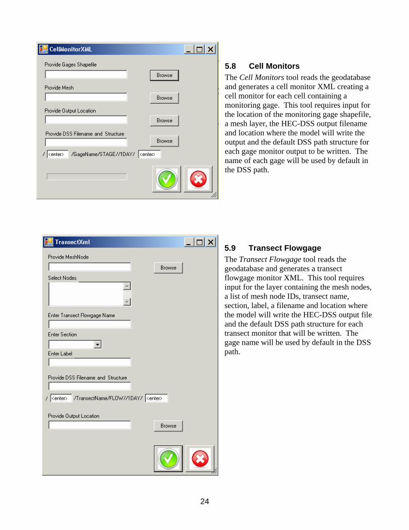
5.8 Cell Monitors The Cell Monitors tool reads the geodatabase and generates a cell monitor XML creating a cell monitor for each cell containing a monitoring gage. This tool requires input for the location of the monitoring gage shapefile, a mesh layer, the HEC-DSS output filename and location where the model will write the output and the default DSS path structure for each gage monitor output to be written. The name of each gage will be used by default in the DSS path.

5.9 Transect Flowgage The Transect Flowgage tool reads the geodatabase and generates a transect flowgage monitor XML. This tool requires input for the layer containing the mesh nodes, a list of mesh node IDs, transect name, section, label, a filename and location where the model will write the HEC-DSS output file and the default DSS path structure for each transect monitor that will be written. The gage name will be used by default in the DSS path.

24

5.10 Levee BC The LeveeBC tool is a simple point and click tool which reads the geodatabase and generates the leveeBC XML file. It will only output information for boundary conditions that are designated as “active”.

5.11 Waterbudget The WaterBudget tool is not currently being used by RSM modelers. It previously was used to generate an XML file that was used to run the RSMBUD tool which is also no longer being used.

5.12 Headstage The Headstage tool is not currently being used by RSM modelers. It previously was used to generate an XML file that was used to run the Headstage tool which is also no longer being used.

5.13 Mesh Attribute The Mesh Attribute tool can output GIS attribute information to a formatted file which is then saved, named as an XML and used as input to the RSM. The mesh attribute file contains header information pertaining to the layer used to supply the information and it contains a sorted list of attribute values. The Mesh attribute tool can be used to create:

• topo.xml • lu_index.xml • bot_lyr.xml • parameter_zones.xml • hyd_con.xml

5.14 Canal File (.MAP) The Canal File (.MAP) tool can output GIS attribute information to a formatted file which is then saved, and used as input to the RSM. The .MAP file contains header information pertaining to the layer used to supply the information and it contains geospatial data descriptions for each segment in the canal network.

25

Figure 14: Canal .MAP Tool (default view) NOTE: This tool MUST be opened prior to opening the geodatabase to be used. This tool will open the geodatabase and it will remain opened after the tool has completed. Opening the geodatabase prior to running this tool will result in the database being locked and the tool will not function properly. The Canal File (.MAP) tool prompts the user to select a canal feature from a geodatabase and the user must also provide an output file location. The tool also offers Advanced Features which use filters to process the selection and then outputs the selected attribute information into an .MAP (ASCII) file.

The Advance Options offers user specified options to modify the information output ot the .MAP file. The default option will output infroamtion for all enabled canals in the geodatabase.

26

Figure 15: Canal .MAP Tool (advanced Options View)

Close any open geodatabases. Start with a blank map. Open an RSM geodatabase. The tool will automatically select the canal layer.

Specify an output location and name for the .MAP file. Click the Advance Options link to view the options. Click OK to generate the .MAP file

27

CHAPTER 6

Utilities There are a number of RSM GIS tools that aid in evaluating and producing output from an RSM mesh. These tools can be found under the Utilities menu on the RSM GIS Toolbar. Features in this menu include the Mesh Suitability test (a.k.a. badness test) and NetCDF Rastor animations.

6.1 Compare Mesh

Figure 16: Compare Mesh Tool

28

6.2 Compare Framework

Figure 17: Compare Framework Tool

6.3 Build NetCDF Rasters

Figure 18: Build NetCDF Rasters Tool

29

6.4 Reporting Triggers

Figure 19: Reporting Triggers Tool

6.5 Mesh Suitability Test

Figure 20: Mesh Suitability Tool

30

CHAPTER 7

Browser Based GIS Tools ArcGIS Server9.2 has been implemented to offer a browser interface to the RSM GIS pre-processing tools. To date GIS server provides a means to examine attributes in a geodatabase and generate the RSM input XML files. As of February 2008, work is underway to migrate the RSM personal geodatabase schema to a versioned SDE geodatabase. This will enable for further development and deployment of the full RSM GIS Toolbar capabilities including the geo-processing tools.

Figure 21: ArcGIS Server 9.2 Application Displaying the C-111 Geodatabase

31

7.1 Arc GIS Server Usage and Capabilities ArcGIS Server is a new package in the ESRI ArcGIS suite of applications. The browser based capability holds very high value for users of the RSM as it allows the SFWMD to web enable the RSM pre-processing tools. To access the current ArcGIS applications use Windows Internet Explorer 7.x or Firefox and navigate to:

http://whqgsrv01d/c111RSM or

http://whqgsrv01d/lecsa_gladesRSM Implemented Tools/Features include:

• Navigation and display of geodatabase layers • Identification and display of layer attribute information • Index Tool (makes several XML files used by the RSM ) • Junction Block XML Tool • Levee XML Tool • Watermover XML Tool

7.2 Uploading an RSM Geo-database At this time users must contact the RSM GUI Development team to upload an RSM geo-database to the ArcGIS Server. In this initial phase, modeling teams will each be given a URL to access their own geo-database. The database can then be shared and viewed by an unlimited number of users on the SFWMD internal computer network.

7.3 RSM GIS Server9.2 Main Navigation Buttons The modeler will use Internet Explorer 7.X or Firefox 2.X to view the main RSM Model page for their geo-database. There are known issue when using older versions of these browsers.

Using your browser navigate to this URL: http://whqgsrv01d/c111RSM The main navigation buttons are located along the top of the main viewing area. They offer buttons to zoom in/out pan, zoom to full extent, identify features, measure distances between features and a magnifier window. Navigation Buttons

Zoom In, Zoom Out, Pan, Full Extent, Identify, Measure, Magnifier

32

7.4 RSM GIS TOOL MENU The RSM GIS tools are organized in a menu along the left side of the browser window where dropdown lists organize the tools into MENU CATEGORIES.

The main menu categories offer tools for: viewing attributes, controlling which layers are viewable, and tools for generating RSM XML files. Each menu can be detached and relocated on the screen as a free-floating menu by clicking on the >> icon. Free-floating menus offer the ability to locate the menu anywhere on the screen and they can be resized. The RSM GUI Tool menu offers a second level of dropdown menus organizing the tools into 3 sub-categories HSE, MSE and XML.

7.5 Results Menu The Results Menu displays output from using the identity button.

Use the Identify button to select a feature in the main viewing window.

A series of expandable lists organize the different levels of information about the features classes retrieved from the geodatabase. Similar to a windows folder system users can navigate by expanding and collapsing the categories by clicking on a series of check boxes to view the levels of information.

33

7.6 Map Contents Menu The Map Contents menu will display the table of contents for the data layers shown on the screen. Layers can be turned on or off by clicking on the box next to each layer name. Each layer in the table of contents can be expanded to display more detailed information about the display settings such as color, line type, etc.

7.7 Navigation The Navigation Menu offers a compass rose which helps navigate within the main map window. Using the mouse, clicking the left button while hovering over the N will pan north. Using the mouse, clicking the left button while hovering over the S will pan south, and so on.

34

7.8 Overview Menu The Overview Menu offers a window showing the present location of the map, relative to the overall extent of the data.

7.9 RSM GUI Tools Menu The RSM GUI Tools Menu organizes the custom GIS tools into groups for pre-processing the HSE canal network, pre-processing the MSE network and for generating XML’s. The groupings are made available through an interface of dropdown menus. These are the primary tools used by modelers preparing an RSM run. The tools extract data from the geodatabase and assemble the information into XML’s formatted for use in the RSM. Header information and comments are also added to the file (where allowed) to self-document the files to aid with post-processing and model output analysis.

XML’s generated from the RSM GUI can easily be identified by the header information and can be traced to the originating geodatabase. Selection of the Index Canal tool will present the user with a sof choices the other XML generating tools are fully autosingle-click tools, and only prompt the user for an output file location. Future development work is expected to expand the

number of tools offered through this interface and completely replace the need for modelers to use ArcGIS desktop or Citrix software.

et mated

The ArcGIS Server deployed tools can be made available to any user, but the ability to upload a geodatabase is expected to be controlled by a smaller set of administrative users who will control the information made available for use through this interface.

7.10 HSE Network Tools Menu

HSE Network Segment Canals Not available at this time. Requires versioned geo-database using ArcSDE.

35

HSE Network Index Canal The Index Tool presents a forms interface for users to selects a GIS Layer and an associated attribute from that layer to generate an Index XML. Typical usage of this tool is for generating the canal_index XML. The user can select from three header formats for the XML which allow this tool to also be used for generating other index files:

• canal_index.dat • hyd_con.xml • lu_index.xml • topo.xml • bot_lyr1.xml

After selecting the desired options the user clicks on the Create Index File button and they are prompted to provide a location to save the resulting XML file.

7.11 MSE Network Tools Menu The MSE Network tools offer assistance in generating two versions of the MSE XML: Complex and Simple. These XML’s are further edited by the modelers to produce an MXML suitable for use in the RSM.

SE

In order for this tool to function there must be water control units (WCU) defined in the geo-database. The MSE XML organizes the attribute information for nodes, segments and junctions in each water control unit.

MSE Network MSE Simple XML Single-click tool used to generate the mse_simple.xml Not available at this time. Requires versioned geo-database using ArcSDE MSE Network MSE Complex XML Single-click tool used to generate the mse_complex.xml Not available at this time. Requires versioned geo-database using ArcSDE

36

7.12 Generate XML Tools Menu The generate XML tools offer several single-click fully automated tools used for generating XML’s for use in an RSM run.

Generate XML Junction Blocks Single-click tool used to generate the junction_block.xml Generate XML Watermover Single-click tool used to generate the watermover.xml Generate XML Levee Seepage Single-click tool used to generate the levee_seepage.xml Generate XML Boundary Condition Single-click tool used to generate the bc.xml

37

CHAPTER 8

The RSM GUI

8.1 Starting the RSM GUI The RSMGUI has been created to organize a set of applications and tools that help modelers with the final steps assembling an RSM scenario, running the model and processing output from the model. The vision for the RSMGUI is to eventually be the single source for all RSM pre- and post-processing. Further development using Arc GIS Server9.2 for pre-processing RSM data will allow us to retire the GIS Toolbar and provide one comprehensive RSMGUI for all RSM user needs. From a Linux PC To run the RSMGUI from any 64bit SFWMD Linux computer, the user must secure shell login to the “whqoom01d” server:

ssh –Y whqoom01d Execute the command to start the RSMGUI:

/opt/local/share3/bin/rsmgui

Optionally users on older computers can run the 32bit RSMGUI by executing the “rsmgui32” command. From a Windows PC Using Xming

Using Xming, start the Xlaunch application using the settings: One Large Window, XDMCP, whqoom01d and accept the defaults to finish the setup.

If you need to have Xming installed contact someone from the RSM GUI Development Team for assistance.

Figure 22: The RSM GUI Python Toolbar The RSMGUI is organized using dropdown menus grouping the (currently 66) features based on the type of function they provide. Typically only one feature can be run at a time. Links under each menu will call open a window to run the selected feature. RSM GUI features are categorized as follows:

• TOOLS: Custom written Python tools • SYSTEM CALLS: calls to Linux system commands • BROWSER LINKS: Links to browser based files (PDF, HTML, etc.) • APPLICATION LINKS: Links to Linux commercial applications (DSSVue, OpenDX, etc.) • GIS SERVER APPLCATIONS: Browser based GIS tools using ArcGIS 9.2 Each feature in the RSM GUI will be explained in this manual.

38

8.2 File Menu

Figure 23: The RSM GUI File Menu The first dropdown menu on the RSMGUI is the File menu. This menu offers only one option, Exit, to exit the RSMGUI. The RSMGUI establishes several environment settings when it starts. Future development is planned to offer interactive settings menus so users can customize their environment and retain preferences within the RSMGUI.

8.3 Exit Feature The most reliable way to quit the RSMGUI is to use the Quit option under the File Menu.

On the RSMGUI under the File menu, select Exit to exit the RSMGUI and to terminate all RSMGUI background processes.

39

CHAPTER 9

PreProcessing Menu

Figure 24: The PreProcessing Menu

9.1 Edit an XML File Tool The Edit an XML File feature calls the nedit utility to edit an XML file. Other text editors are available within Linux but nedit is one of the more basic and simple to use.

Other editors you may like to try are: gedit, xemacs, and kedit

9.2 Scenario Builder Tool The Scenario Builder gives assistance in generating blocks of XML assembled from manual user input, reading input files and from user selections from dropdown menus. There are 22 features in the Scenario Builder. The RSM employs a very open and highly customizable framework. XML input files must adhere to rules and are expected to contain certain information but they can be assembled and combined to create an endless variety of configurations. To help modelers create their XML files the GUI offers a means to generate blocks of XML. These XML blocks can be saved as files or copy and pasted into other XML files. The MAIN XML, which refers to the XML used to run an RSM scenario, has several customizable blocks. The scenario builder helps assemble several of the blocks so they can be quickly generated and assembled together. At a minimum this tool helps generate consistently formatted XML blocks that are readable, contain and it helps avoid typing errors over creating and XML entirely by hand.

On the RSM Toolbar under the Pre-processing menu select the Scenario Builder tool.

40

Figure 25: Scenario Builder Tool

9.2.1 Entity The Entity Tool generates the <entity> portion of the MAIN XML. This block of XML specifies the associated files used to create the RSM. Entity is similar to an <include> statement as used in other mark-up languages. Users can browse to a file for the pre-specified entities or 6 custom entities can be created where users can browse to a file and specify their own entity names. A relative path can be typed in or by browsing the literal path will be captured also verifying the existence of the file. Once browsed to the path can be edited to form of a relative path. The READ FILE button will read and generate entities from an existing XML. The GENERATE OUTPUT button will generate the output form this tool.

41

42

9.2.2 Control The Control Tool generates the <control> portion of the MAIN XML. This block of XML specifies the options used to run the RSM. By choosing form dropdown list, radio button and selcting options the user can avoid time consuming mistakes of typing incorrect options or incorrect format. The READ FILE button will read and generate control settings from an existing XML. By using this tool the order by which the control settings appear in the XML will be consistent and easier to read by modelers who are familiar with these standard settings. The GENERATE OUTPUT button will generate the output form this tool.

43

<MESH>

9.2.3 Conveyance Tool Writes: conveyance.xml The conveyance tool reads in an existing XML containing a conveyance xml block and extracts jus the conveyance block and presents the data for viewing and editing. Conveyance consists of one index file.

44

9.2.4 Svconverter Writes: svconverter.xml The svconverter reads in an existing svconverter xml and presents the data in an easy to navigate menu for viewing and editing. Svconverter consists of one type or a mix of types such as: confined, unconfined, unconfined_gms_layer, or layered. This tool utilizes the DTD to ensure proper formatting for each type present in the XML

9.2.5 Transmissivity Tool Writes: transmisivity.xml The transmissivity tool reads in an existing transmissivity xml and presents the data in an easy to navigate menu for viewing and editing. Transmissivity can consist of one type or a mix of types such as: confined, unconfined, unconfined_gms_layer, or layered. This tool utilizes the DTD to ensure proper formatting for each type present in the XML.

45

46

<Network> The network XML assigns all the information pertaining to the canal network such as: geometry, initial stage conditions, network boundary conditions, segment sources, junctions, and connectivity.

9.2.6 arcs (xsentry) Writes: arcs xml This RSMGUI tool reads the main XML, acquires xsentry and parses it for editing.

<Controllers>

9.2.7 MSE Controllers Writes: controllers.xml This RSMGUI tool reads the MAIN XML, acquires MSE Controllers and parses them for editing.

47

<Output> The output tools assist with creating XML blocks for generating output from the RSM by placing them in the <output> section of the MAIN XML.

9.2.8 BC Monitor This RSMGUI tool reads the BC XML, acquires information for every boundary condition and generates the BCMONITOR XML block. Users are prompted to specify the DSS output path and the default fields in the HEC-DSS path. The BC label is automatically used for field 2 in the DSS path to help identify each boundary condition.

48

9.2.9 Cell Monitor This RSMGUI tool generates the CELL MONITOR XML block. Users are prompted to enter a list of cell IDs or a list can be read in from a file containing a single column of IDs. Users are prompted to specify the DSS output path and the default fields in the HEC-DSS path. The cell ID is automatically used in the id for each cell monitor. The DSS path can be hand edited to make a unique DSS path for each cell monitor.

49

9.2.10 Flowgage This RSMGUI tool generates the FLOWGAGE MONITOR XML block. Users are prompted to enter a list of node IDs or a list can be read in from a file containing a single column of IDs. Users are prompted to specify the DSS output path and the default fields in the HEC-DSS path. The DSS path can be hand edited to make a unique DSS path for each flowgage monitor.

50

9.2.11 Global Monitor

9.2.12 Impoundment Monitor

9.2.13 Junction Monitor

9.2.14 Segment Monitor

51

9.2.15 Waterbudget Output

9.2.16 WCD Monitor

9.2.17 WCU Monitor

9.2.18 WM Monitor

52

9.3 PWS XML Tool The Public Watersupply Well XML (PWS XML) tool helps build the public water supply XML. This tool reads in a list of well ID’s, a list of cell ID’s, offers a means to set attributes for the PWS XML and then generates a well XML block.

On the RSM Toolbar under the Pre-processing menu select the PWS XML Tool.

Figure 26: PWS XML Tool and PWS XML file

Click the Read File button. Select /opt/local/share3/share/samples/pws/pws_inputfile.csv Click the generate Output button.

53

9.4 Rulecurve XML The Rulecurve XML tool helps build a rule curve XML. This tool prompts the modeler to first generate a generic rule or standard wet/dry season curve. The user is prompted to set the ID, label and units for the rule curve and then provides inputs start/end for each elevation. After a rule is finished additional rules can be added to the same XML. The output is a rulecurves XML with one or many rc entries.

Figure 27: Rule Curve Tool

9.5 Reverse Engineer The Reverse Engineer tool was created to traverse an RSM Main XML and generate containing all references to GIS attributes that are present in the XML (an included XMLs). There has been very limited use of this tool, redesign is being considered and no sample data is available.

Figure 28: Reverse Engineer Tool

54

9.6 Chloride SQL to DSS The Chloride SQL to DSS tool was created to help users extract chloride data from Oracle and export it to a HEC-DSS file to be used as model input. The user provides a control file consisting of comma delimited rows of permit numbers and station IDs. Output options include choices to interpolate missing data, output to HEC-DSS, ASCII or to generate graphs in PDF format. PDF graphics can be displayed automatically when the tool completes the operation.

Sample control file : 06-01474-W, 41584

9.6 DBHYDRO SQL to DSS B s created to help users extract data from DBHYDRO and export it

ut to

Sample control file:

06-01474-W, 19644

The D HYDRO SQL to DSS tool wato a HEC-DSS file to be used as model input. The user provides a control file consisting of signle column of DBHYDRO DBKEYs. Output options include choices to interpolate missing data, outpHEC-DSS, ASCII or to generate graphs in PDF format. PDF graphics can be displayed automatically when the tool completes the operation.

06-01474-W, 41584 06-01474-W, 19644

55

Chapter 10

Run Model Menu

Figure 29: The Run Model Menu After all files have been assembled the model can be run via the Run Model menu on the toolbar. The Run Model interface offers input options to browse to the compiled HSE version of the model, the calibration XML to be used to control the scenario and it also has optional comment fields to help catalog the model run. Statistics from each run are captured and stored in the Model Log, which can also be found under the Run Model menu on the toolbar.

10.1 Run Model Tool The Run Model tool provides an interface to help run the model, capture information about the run, and send an email notification when the run is completed successfully.

Figure 30: Run Model Tool The input files for a scenario are typically stored on dcluster1 (whqoom01d) under the workdirs directory. The model directory will contain an input and output subdirectory. In addition the modeler will specify the location of a compiled version of the HSE to be used to make the run. The MAIN XML controls how the scenario will be executed. The MAIN XML contains references to the DTD (data type definition) file, the location and names of the input files, the location and names for output files, and all externally referenced files.

56

Features in the Run Model tool include: • XML File: the MAIN XML to be used to make this run. • Model Executable Path: the compiled HSE executable • Reason to Run Model: optional comment to document the reason for making this run • Comments: optional comments about this run • Select Existing Region Name: select the region (names) for this run from a dropdown list of

previously made runs • Enter New Region Name: input the region (name) for this run and it will be added to the dropdown

list for future use in this tool • Send Email: email address where an automated email notice will be sent upon completion of the run • Run Locally: execute this run on the server where the RSMGUI is being run • Run On Cluster: execute this run on the compute cluster dcluster1

See Appendix D for a description of all the files used to execute a sample RSM implementation.

10.3 Parameter Sensitivity Tool The parameter Sensitivity tool provides a means to prescribe a value range for a parameter to be tested, execute up to 10 runs of the RSM, capture output the test results into a DSS file and plot a graph comparing the results. The model implementation can be modified, executed and analyzed using this tool. The user provides the location of the MAIN XML and the path the HSE executable.

The user is then presented with a choice of variables that can be tested in the run. The user can click on the first variable shown in the text box and then a selection window will open giving the user a choice from all variables found in the run.

57

After the variable has been selected, the next menu gives a choice of the parameters associated with the chosen variable. Valid variable types and parameters include:

Variable Parameters Mannings a, b, detent Leakage_coeff coeff Seepage_coeff coeff

The next menu allows the user to prescribe a range to be tested for the chosen parameter by selecting a min and max value. Increments can be set by specifying the increment or by choosing the number of runs to be made and letting the tool calculate the increment. The user then creates a monitor to capture and compare the results. Users must be familiar with the RSM implementation being run in order to know what monitor will be impacted by the parameter being tested. Options include creating a cell_monitor, segment_monitor, junction_monitor, or a wm_monitor. The monitor can be set for the default time of the model or a longer timeframe (dbintl) and the resulting DSS file can be saved to a named location. A browse button helps locate a suitable location and then the user is expected to enter a desired name for the resulting file that will contain the data for each parameter interval to be tested.

The final menu displays the settings for the model run(s) to be made: Path the main XML, Path the HSE, Variable name, Parameter name, Parameter min & max, Number of runs to be made and the Parameter increment. The user can also enter optional information about the run and choose to have an email sent to an address when the runs are complete. The run can be executed locally where the RSMGUI is being run from or on the DCLUSTER if the user is on the SFWMD network and the run is stored on the Storage Area Network (SAN).

58

NOTE: DCLUSTER runs must be made using a model that is on the SFWMD network and is stored on the Storage Area Network (SAN).

Figure 31: Output from Parameter Sensitivity Tool

59

10.2 View Model Log After a run has been made using the Run Model tool, information about the run is stored in a Model Log file. If the RSMGUI is run while off of the SFWMD network, the model log file is stored locally and then copied to the RSMGUI Master Model Log the next time the GUI is started while the computer is connected to the SFWMD network. The Model Log can be searched using the following options: • All Users: this will display the entire Model Log. • Single User: enter the name of a user in field provided to search for runs made that user • Region Name: select the name of a region from a dropdown list to search for runs associated with

that region • Display: execute the search • Cancel: dismiss the tool\ •

Figure 32: Interface Used to Search the Model Log

60

Figure 33: Sample Output from the Run Model Log Additional system information is captured when the RSM runs are made using the Run Model tool. Information is captured pertaining to two different areas about the run, System Information and Model Information.

System Information: • Name of the user who made this run • Execution start date/time • Execution end date/time • Elapsed system execution time • Server name

Model information: • Path to the HSE used • Path to the MAIN XML used • Model simulation start date & time • Model simulation end date/time • Budget package invoked (yes or no) • Region name

61

Chapter 11

View Model Results Menu

Figure 34: The View Model Results Menu

11.1 Results Viewer The Results Viewer feature is a Python tool. It contains over 33 features organized with its own system of dropdown menus. This is one of the earliest GUI tools developed for the RSM. A Help Menu within the Results Viewer provides detailed instructions on usage for many of the features it contains. When the Results Viewer first starts it prompts the user for an RSM netCDF file. Optionally, a second netCDF file can be specified and a GIS shape (.shp) file can be specified to be displayed along with the netCDF data.

Figure 35: ResultsViewer start-up interface After specifying the netCDF file(s) the user clicks the Run button and three display windows will open on the screen: • The main window (canvas) will display the mesh • The Time Navigator Window offers buttons to move forward and back in the timesteps • The Info Window displays information about the data being displayed on the screen.

Run the ResultsViewer tool using: /opt/local/share3/share/samples/results_viewer/C111_PIR1_Alt2Db.nc

Under the View menu check the box next to Flow Vectors. Under the Tools menu Change the Change Flow Vector Grid Size to 50.

62

It may be necessary to move the windows on the screen to view all three at the same time.

Figure 36: Results Viewer Display Windows

63

The following is an inventory of the features available in the Results Viewer: File Menu:

• Export – export screen captures of the main display window

View Menu • Zoom – zoom in/out (also works using: page-up, page-down) • Flow Vector – display flow vectors from the netCDF which are created by using the

<globalmonitor attr=“olvector”> output option. • Legend – display a legend for cell colorflood shading

Cells Menu

• Show Cells – non-functioning feature • Cell Colorflood – displays colorflood of ponding depth or computed head elevations

Segments Menu • Show Segments – non-functioning feature • Segment Color flood - non-functioning feature

Tools Menu • Digitize ROI – select a Region of Interest (ROI) to only colorflood a sub-region of the model • Cell Colorflood Tools - non-functioning feature • Time Tools – Display the time navigator and the time converter • Misc Tool – A collection of tools to display a colorflood Movie, Calibration, Hydrographs,

Segment Viewer, Summary Statistics, and a Pest Visualization tool. • Segment Colorflood Tools - non-functioning feature • Change flowvector Grid Size – Change the size of the grid which is overlayed on the mesh to

select the flowvector arrows to be displayed. Help Menu

• Show HTML Help – displays an HTML help manual for the features in the Results Viewer

11.1.1 Pest Visualization Within the Results Viewer there are 2 features to help visualize PEST output. These tools display Jacobian Matrix (.jco) and Correlation Matrix (.rec) output from PEST.

Figure 37: Pest Visualization Options Menu

At the top of the Results Viewer main window, select the Tools Menu Select the Misc Tools Option Select the Pest Visualization Tool

64

Select to view the corresponding Jacobian or Correlation Matrix file from the NC file you are viewing in the Results Viewer

Select to view the file: /opt/local/share3/share/samples/results_viewer/bbw_95_jsc.jco

Select to view the file: /opt/local/share3/share/samples/results_viewer/bbcw_9.rec

Figure 38: Viewing Jacobian Matrix Output from PEST

Figure 39: Viewing Correlation Matrix Output from PEST

65

11.2 ncBrowse The ncBrowse feature is an application link to the ncBrowse application written by the National Oceanographic & Atmospheric Administration (NOAA.) ncBrowse is a netCDF binary file browser utility. http://www.epic.noaa.gov/java/ncBrowse/ Command Line Option: /opt/local/share2/bin/ncBrowse

Select to view the file: /opt/local/share3/share/samples/nc_diff/C111_Alt6-Base_94-95.nc

Select the to view the ComputedHead variable from the list on the right (double-click)

The settings window will appear. Change the start value for cells to be the same as the end value (3544) Click the Graph Variable button to view a hydrograph for waterbody ID 3544.

Figure 40: ncBrowse Tool

11.3 HecDSSVue The HecDSSVue feature is an application link to the Hydrologic Engineering Center’s Data Storage System Visual Utility Engine (HecDSSVue) application written by the U.S. Army Corps of Engineers (USACE). HecDSSVue is a DSS binary file browser utility. http://www.waterengr.com/HECDSSVue/hecdssvue.html Command Line Option: /opt/local/share2_64/bin_32/dssvue

66

Figure 41: Hec-DSSVue Tool

11.4 DSSMapVue The HecDSS MapVue feature is an application link to the Hydrologic Engineering Center's Data Storage System Mapping Visual Utility Engine (Hec-DSS MapVue). Command Line Option: /opt/local/share2/bin/dssmapvue

Figure 42: Hec-DSS MapVue Tool MapVue ver 1.0 for Linux has been installed based on a request by Ruben Arteaga. No other information is available on the usage of this tool.

67

11.5 OpenDX The OpenDX feature is an application link to Open Visualization Data Explorer (OpenDX). OpenDX is an opensource application used by RSM modelers to view netCDF output files and display 3D animations. http://www.opendx.org/ Command Line Option: /opt/local/share2/bin/dx

After Open DX starts click on the button to “Edit Visual Program”. Open the file “/opt/local/share3/share/samples/open_DX/pretty_plot.net” A graphic window will open displaying the pretty_plot.net program. Within the graphic window double-click on the icon labeled as “Import” On the right side of the menu make sure:

o the file name is “/opt/local/share3/share/samples/open_DX/bbw_test.nc”

o variable is set to “ComputedHead” o format is set to “netCDF”

Click the “Apply” button Click the “OK” button Select Execute from the top menu choices in the graphic window Click on the choice called “Sequencer” Click the Play button “ ”in the sequencer to start the animation.

68

Figure 43: Open_DX Graphic Window Open DX Sequencer

69

Figure 44: Open_DX Animation Output

11.6 Cell Comparison Hydrographs The Cell Comparison Hydrograph feature is a Python tool under the View Model Results menu. This tool has been created to provide an easy means to compare indicator cells from 2 or 3 model runs from the same implementation. The tool accepts 2 or 3 Globalmonitor netCDF files which must contain HEAD and TOPOGRAPHY global monitor output or optionally PONDING output can also be used. The final result is a hydrograph and a duration curve for each selected cell.

Using the Cell Comparison Tool The first input menu captures the location of 2 or 3 globalmonitor netCDF files and a name for each one which is used to create the legend in each graph.

70

The second input menu captures the cell IDs and a title for each graph. Cell IDs can be entered by clicking in the text field and selecting an ID form the dropdown list of cells found in the netCDF file. Additional cell IDs can be added by clicking the [Add Another ID] button and they can be removed from the list by clicking on [Delete ID] button next to each line. The file must contain the cell ID and Main Title separated by commas. Sample input file: cellid,gage 308, Sawgrass Gage 724, Ridge and Slouge Gage #1 854, Ridge and Slouge Gage #2 Users can select from the Chart Type dropdown menu to choose the variable to be used to create the hydrograph. The duration curve will only display Ponding Depth. If the globalmonitor file does not include ponding output, the pondingdepth will be calculated by subtracting (Computedhead – Topo). This may result in negative (below land surface) ponding values.

The globalmonitor netCDF file MUST contain HEAD and TOPO output.

<output> <globalmonitor attr="ponding">

<netcdf file="globalmonitor.nc"></netcdf> </globalmonitor> <globalmonitor attr="topo"> <netcdf file=" globalmonitor.nc"></netcdf> </globalmonitor> <globalmonitor attr="head"> <netcdf file=" globalmonitor.nc"></netcdf> </globalmonitor> </output> Optionally, the hydrograph can be displayed on one graph for the period of record or it can be split into 2 graphs on one page by clicking on the Split hydrograph button. A title block can be created by adding text into the Title Block field. The title block will appear in the lower right corner of each output page. A maximum of 3 lines should be used for the title block but usage of this feature is optional. There are 3 color choices for the title block (blue, black, green, red).

71

Figure 45: Cell Comparison Hydrograph Tool

11.7 Waterbody_CAT The Waterbody_CAT feature is a Python tool. This tool is used to display waterbody data from a netCDF file in tabular format. The tool prompts the user for a netCDF input file, extracts a list of waterbody IDs the user then selects an attribute type to include in the (.csv) report. The user also has an option to generate a GMS formatted file. The netCDF can be a budgetpackage or wbbudgetpackage file.

Select to view the file: /opt/local/share3/share/samples/waterbody_cat/BM54_compbudget.nc

Select to view the Cell waterbody type, then click Next Select waterbody ID 1, Select Time Series Variable Type, then click Next Select the WBStorageVolume Attribute Type, click on Generate Report

The final report from Waterbody_CAT includes a header, summarized daily, monthly, annual min/max/mean/sum values and is CSV formatted for importing into Excel.

72

Figure 46: Waterbody_CAT Tool

11.8 Waterbody_PLOT The Waterbody_PLOT feature is a Python tool that is very similar to Waterbody_CAT but it generates a plot from the selected netCDF data rather than a report. The output is in PDF format.

Select to view the file: /opt/local/share3/share/samples/waterbody_cat/BM54_compbudget.nc

73

Figure 47: Waterbody_PLOT Tool

11.9 Watermover_CAT The Watermover_CAT feature is used to extract and tabulate a watermover data report from a netCDF file. The tool prompts the user for a wbbudgetpackage netCDF file, extracts a list of waterbodys to choose from. The tool then extracts a list of watermovers and timesteps associated with the selected waterbodies. The user selects the watermovers they wish to report and they select a start and end timestep. There are also options for summarizing monthly, annual or seasonal reports.

74

The tool generates a report (.csv) report showing the data for the selected watermovers in a column CSV formatted file suitable for viewing in a spreadsheet for analysis.

Select to view the file: /opt/local/share3/share/samples/watermover_cat/wbbudgetpackage.nc

Select a watermover from the list of watermovers by clicking on it Select a beginning and ending timestep Click the Execute button, the tool will generate a report.

75

Figure 48: Output from the Watermover_CAT Tool

11.10 Watermover_PLOT The Watermover_PLOT feature is a Python tool that is very similar to Watermover_CAT but it generates a plot from the selected netCDF data rather than a report. The output is in PDF format.

Select to view the file: /opt/local/share3/share/samples/watermover_cat/BM54_compbudget.nc

76

Figure 49: Watermover_PLOT Tool

11.11 Google KMZ Animation The Google KMZ Animation feature is a Python tool that generates a KMZ file that can be viewed using GoogleEarth. This tool uses information from an RSM netCDF file and two files output from GIS to help draw the mesh. The files from GIS provide a base mesh KML file to draw the RSM mesh and a cross-walk file to help translate the mesh object IDs to cell IDs. The KMZ file can be used to display timeseries animations showing ponding depths, computedhead elevations or flow vector arrows. The tool prompts the user for 3 files: • NetCDF file: a netCDF file containing global monitor data for Ponding or ComputedHead and/or

totalvector • mesh KML file: a KML file generated from Arc2Earth tool in GIS containing the information to

draw the mesh. • Cell ID crosswalk file: an ASCII (.csv) file containing 2 columns of data (cell objID, cellID) After the files are read, a menu then offers configuration options for building the KMZ file. Options include: • Date Range: change the start/end date for the animation. • Timestep type: generate timesteps based on a selected increment (1=every value), or day of the

month (31=end of the month for all months). • Data on/off: include display of cell ID in the KMZ file

77

• Flow Vectors on/off: generate a layer with flow vector arrows in the KMZ file, (will only work if totalvector is in the netCDF file)

• Flow Vector Grid: flow vector arrows are generated based by overlaying a square grid (25x25 default) on top of the mesh

• Color Ramp Range: 2 pre-set ranges can be used for colorshading the cells or a min/max value can be manually entered. 20 increments are calculated and assigned a pre-set color.

• Output Dir: specify the location for the resulting output file. The name will be generated based on the name of the netCDF file.

• Mesh Type: select the mesh attribute to animate Select the following 3 files to test this tool:

o /opt/local/share3/share/samples/googleearth/bbcw-calib.nc o /opt/local/share3/share/samples/googleearth/bbcw-mesh.kml o /opt/local/share3/share/samples/googleearth/bbcw-crosswalk.csv

Select a date range of 1983-01-01 to 1983-01-05 Set Data = off Set Flow Vector = on Set Grid = 25 Set color Ramp Range = Large Specify a location to save the KMZ file. Set Mesh Type = ComputedHead

Click the Build Mesh Animation button to run the tool.

The tool will generate an alert when it is complete and give a reminder on where the output file was saved. If a file already exists with the same name the tool will pause and prompt to overwrite the file.

Open Google Earth and view the KMZ file.

DO NOT try to create a KMZ file with more than 30 timesteps. The file size will likely exceed the memory limits of GoogleEarth.

78

Figure 50: Google Earth Tool

It may be necessary to open the mesh.kml generated by Arc2Earth inside GoogleEarth, save it as a new file and then use the new file as input to this tool.

A sample KMZ file for viewing in GoogleEarth is available at: /opt/local/share3/share/samples/googleearth/bbcw-calib-mesh.kmz

Start Google Earth and view the KMZ file. GoogleEarth offers controls to play the animation, speed-up, slow-down, zoom in/out, rotate, and tilt the landscape perspective.

79

Figure 51: GoogleEarth KMZ Animation Showing ComputedHead Elevations in 2D While viewing the Google Animation users can click on any cell and select to view the hydrograph which is generated from the model output netCDF file. The first time the hydrograph option is selected a browser window will appear in the Google Earth window and the user must specify the location of the netCDF file to be used. The tool will then remember the file location to be used for viewing other hydrographs from the same file. The hydrograph will appear in a separate browser window where it can be viewed or saved to a location specified by the user. The hydrograph is presented in PDF format.

80

11.12 Transect Tool The Transect Tool is a Python tool used to report flows across transects by reading global monitor information from either a budgetpackage or wbbudgetpackage netCDF file and a file containing a list of mesh node IDs. This tool generates a report similar to the output generated by the RSM when transect monitor output is specified in the MAIN XML. If a transect monitor is desired after completing an RSM run, but it was not specified at the time the run was made, the only alternative was to re-run the model. With a wbbudget netCDF file a transect flow report can be generated for any transect in the model. The mesh nodes define the location of transect. The tool analyzes the netCDF file, extracts the flows across the specified transect and then generates 4 reports:

• Transect Report • Daily Report

81

• Monthly Summary Report • Annual Summary Report

The list of mesh nodes specified by the user is printed at the top of each report [1 6 11 16]. The corresponding IDs in netCDF file have an offset of (-1). Mesh node IDs are selected form the “triple” array in the netCDF file which have IDs that are offset by (-1) from the mesh node IDs used in the RSM geodatabase. The IDs gathered from the netCDF are listed for verification: wall [0 5 10 15]. To generate transect flow output form the RSM this output option must be included as part of the RUN XML to generate similar output as seen in this example.

Specifying transect output in the RSM: <flowgage section=”ol_gw” label=”Transect_olgw”> <nodelist>1 6 11 16</nodelist> <asciiform file=”./Transect_olgw611.txt” format=”%10.6f”></asciiform> </fowgage>

Figure 52: Output from the RSM GUI Transect Tool

Run the tool using these sample files: /opt/local/share3/share/samples/transect/compbudget.nc and nodelist.csv

This tool has been tested using output from ver. HSE2.0.0, 32-bt, 64-bit and against wbbudgetpackage output.

82

Chapter 12

Process Model Output Menu

Figure 53: Process Model Output Menu

12.1 Waterbudget Residual Animation The Waterbudget Residual Animation feature is a Python tool that generates a timeseries animation of the model using colors to symbolize the amount of residual for each mesh cell. The tool requires a composite budgetpackage netCDF output file and a wbbudgetpackage netCDF output file. It offers a menu with options to specify how the animation should be formatted. The user is prompted to select waterbody IDs, choose a date range and is given options to control the format of the report. The composite waterbudget report is a combination of waterbody volumes and HPM volumes which should produce a balanced (less than 10-4 discrepancy) report. Format options for the Waterbudget Residual Animation tool include: • Save Pathname: specify an output location for the output animation • Show Mesh Border: outline the mesh cells in the animation • Animate Cells: animate each cell • Animate Segments: animate each segment • Colorflood min/max: specify a range to assign 20 color variations • Timestep Increment: specify a timestep interval to animate (ie. every 5th timestep) or specify a

certain day of the month (ie. the 1st day of each month) • Start/end date: select a start and end time range to animate

83

Figure 54: Waterbudget Residual Animation Input Options Output form the Waterbudget Residual Animation tool is in the form of PNG images that can be viewed in an HTML viewer using any browser. The animation viewer has controls to stop, start, go forward, and to go back. Play speed can be adjusted by specifying the duration each frame will be viewed (1000 milliseconds = 1 second). The display also includes a color legend, the timestep being viewed and meta information documenting the units, file name and variable being displayed.

Select the Map netCDF file: /opt/local/share3/share/samples/C111/CERP_Alts/output/SR5_sss/waterbudget_C111_SR5_sss.nc

Select the Waterbudget netCDF file: /opt/local/share3/share/samples/C111/CERP_Alts/output/SR5_sss/composite_budget_C111_91_94-95.nc

Specify an output directory where you would like to store the output Unclick the Show Mesh Borders option Click the Animate Cells option Specify a 0 to 35 colorflood range Select a timestep increment of 1 Select timestep 0 as the start and timestep 9 as the end timestep Click generate to create the waterbudget residual animation

84

Figure 55: Output from the Waterbudget Residual Animation Tool

12.2 NCDump The NCDump feature is an application link to the Unidata ncdump application. ncdump generates an ASCII report from a specified netCDF file. The user is prompted to supply the location of a netCDF file and output is generated to a display window. http://www.unidata.ucar.edu/software/netcdf/docs/ncdump-man-1.html

12.3 List of Mesh Cells The List of Mesh Cells feature is a Python tool. This tool is used to display a list of Cell IDs contained in a netCDF file. The tool prompts the user for a netCDF input file and extracts a list of cell IDs from the file.

Select to view the file: /opt/local/share3/share/samples/nc_diff/C111_ALT-Base_94-95.nc

Click Get Cell Ids and a list of cell IDs in the netCDF file will be displayed (1-3584 in this example).

Output from this tool can be saved to a file.

85

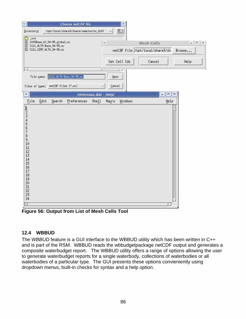
Figure 56: Output from List of Mesh Cells Tool

12.4 WBBUD The WBBUD feature is a GUI interface to the WBBUD utility which has been written in C++ and is part of the RSM. WBBUD reads the wbbudgetpackage netCDF output and generates a composite waterbudget report. The WBBUD utility offers a range of options allowing the user to generate waterbudget reports for a single waterbody, collections of waterbodies or all waterbodies of a particular type. The GUI presents these options convieniently using dropdown menus, built-in checks for syntax and a help option.

86

WBBUD Options include: -a: report a summed report for all waterbodies of the specified type -s: report a summed report for a subset (list) of waterbodies either provided in a file or entered by hand. -m: Multiply the output (ie. –m 12 to convert inches to feet) -u: Units to be displayed in the header (required field if using the multiplier option) -v: Verbose expanded output. -c: Condensed report -t: Transform output to volume, rate or Depth -f: Format the report to summarize all (raw) data, daily, monthly or annual -j: Julian date conversion The GUI requires a location and name for the output file that will be generated. There is also an option to immediately display the output when the report is generated.

Select to the file: /opt/local/share3/samples/C111/CERP_Alts/output/SR5_sss/

wbbudget_C111_SR5_sss.nc Select the Subset option Enter 19 in the IDs Subset input box Multiplier should be set to default value of 1.0 Units should be left blank Enter a path and file name in the output box Select the Verbose option Select the Volume transform option Select the Day format option Disable the Julian option Click Next>>> The output will be written to the output file and a window will prompt the user to view the file that has been written.

wbbud can be run from the command line by using the wbbud utility located in trunk/src/budtool/wbbud

Figure 57: WBBUD Main Options Menu

87

Figure 58: Output report from WBBUD for waterbody 19

12.5 NC Difference Tool The NC Difference feature is a Python tool that calculates the difference between to netCDF files and generates a new netCDF. This tool was created to help analyze the difference between two RSM alternative runs. Two netCDF files are read, the difference is calculated for the selected attribute and the new netCDF file is written. Users are prompted to provide the location of an alternative netCDF file, a base netCDF file and the location where the new netCDF file will be written. The tool calculates the difference: Alt – Base = newfile The user can specify to calculate the difference between PondDepth or ComputedHead. Variable sin the netCDF file.

Figure 59: NC Difference Tool Menu

88

Select to use the files:

/opt/local/share3/share/samples/nc_diff/C111_ALT-Base_94-95.nc 2005Base_AJ_94-95_global.nc

Provide an output location where the resulting new file can be written Click merge the PondDepth variable

12.6 Dynamic Charting Tool The Dynamic Charting feature is a Python tool that provides an interface for users to chart data from DSS and/or netCDF output files and dynamically change the charting options to achieve the desired output graphic. This tool is inteneded to be a precursor to creating new performance measure graphics allowing the user to specify data, change legends, titles and line symbols. Users are presented with an interface that prompts for an existing control file or it will assist users in creating a new graphic and save the control file when it is completed. The main menu offers numerous options to select and display data sets.

Figure 60: Dynamic Charting Tool Initial menu

89

The main menu screen offers options to open an existing settings file, start a new session. Once an existing control file is open the user can:

• directly edit the text in the file • Save the control file to a new name/location • Export data specified in the control file to a CSV file • Export the graphical output resulting from use of the control file to a PDF file • Open the GUI to modify the control file • View the graphical output. • View the tabular data resulting from use of the control file

Figure 61: Dynamic Charting main settings menu Once an existing control file is open the user can open the GUI to modify the control file, directly edit the text in the file or choose to view the graphical output. Options in the GUI allow users to:

• Set the data date range • Set the Y-axis range • Control display of tick marks • Set titles, y-axis and x-axis titles • Specify location and size of the legend • Control display of grid lines

90

• Add/remove (DSS or NC) data sets to be included • Control display of each data line

o Line weight o Line color o Line symbol o Legend text o Order datasets are shown in the legend

Figure 62: Dynamic Charting sample output

91

Figure 63: Dynamic Charting settings file 12.7 EFDC Structure Translator

In order to support and promote use of output from the RSM this tool has been created reformat RSM output data into a format readable by the SNOOK model reader being used by Michael Kohler and CERP. NetCDF output form the RSM is read and reformatted into either a structure data set or a headstage dataset. Output from this tool is a binary file and an ascii file. The EFDC Structure Translator translates data for the structure watermovers from the RSM <wbbudgetpackage> and produces an ascii (.dat) file and a binary (.bin) file. The files contain a column of data for each structure in the netCDF file.

92

Output from this tool is presented in a browser offering a hypertext link to the binary and ascii file.

12. 8 EFDC Headstage Translator The EFDC Headstage Translator tool translates computedHead stage data from the RSM <globalmonitor attr=”head”> and produces an ascii (.dat) file and a binary (.bin) file. The files contain an array of data for each waterbody in the netCDF file.

12.9 Tecplot Loader <information to be added in next release>

93

Chapter 13

Output Graphics Menu

Figure 64: Output Graphics Menu

Several of the tools found under the Output Graphics menu use CONTROL FILES as input. These are ASCII text files designed to contain references to data files, titles and other formatting information that help control the specific application being run. The HELP button on each RSM GUI tool contains a reference where a sample control file can be found. Where it is helpful, these instructions reference how to create each control file. Control File This example control file demonstrates how “file” is used to indicate a line containing references to data files. In this case there are 3 files references by using relative paths from where the control file is located. The second line uses “run” to indicate this is a line containing references to dss data for a particular model run. In this case there are 3 DSS data paths which will be retrieved form the 3 files listed on the “file” line. The first string of text after the “run” is CH_EVER1 which is the name of this dataset and it will be used in the main title of the plot. file ./output/glades_lecsa_output.dss ./output/struct_flow.dss ./output/struct_flow.dss run CH_EVER1 /GLADES_LECSA/EVER1/STAGE//1DAY/SIMULATED/ /SFRSM/S2/STAGE//1DAY/CALC/ /SFRSM/S3/STAGE//1DAY/CALC/

94

13.1 DSS Stage/Flow Plots The DSS Stage/Flow Plots feature is a Python tool that reads DSS output from the RSM and produces flow or stage comparison hydrographs. The output also includes statistics comparing the RSM and SFWMM output. The tool reads in a CONTROL FILE which contains references to the DSS files and DSS data paths to be plotted.

Figure 65: DSS Stage/Flow Plots Input Menu

Select to use the file:

/opt/local/share3/share/samples/dss_plots/sample.ctl Click to output the Graphs Accept the default start and end dates Click the Generate button to create the DSS Stage/Flow Plots

Figure 66: Output from DSS Stage/Flow Plot Tool

95

13.2 NetCDF Stage/Flow Plots The netCDF Stage/Flow Plots feature is a Python tool that produces a series of 4 plots showing RSM flow and stages for comparison with SFWMM model output. The output also includes statistics comparing the RSM and SFWMM output. The tool reads in an RSM netCDF file and it reads in an OBSERVED CELLS XML file. The OBSERVED CELLS XML file contains information linking DSS data for each gage to a cell in the model. Users are offered options to generate output graphics, CSV tabular data or both. The user can also select to output all 4 graphics or one type.

Select to use the file: /opt/local/share3/share/samples/netcdf_plots/broward_bm.nc and obs_cells.xml

Sample CSV file can also be found in this location: /opt/local/share3/share/samples/netcdf_plots/stageCV_v1.csv Observed Cells File The observed cells XML contains an <observations> element which contains a link to a file (stageCV_v1.csv). The XML also contains an <observation> entry for each gage to be used by the netCDF Flow/Stage tool. The station name and id are used to retrieve the associated stage/flow data from the model NC file and DSS files containing the historical and SFWMM comparison data. <observations start_date="1991-01-01" end_date="1995-12-31" > <!-- Gages outside of canal --> <file name="stageCV_v1.csv" type="csv" missing_value="-901.0" key="stageData" />

96

<observation name="G2030" description="G2030, Well" stationname="G2030" type="cell" id="13439" variable="ComputedHead" weight="1.0" file="stageData" />

Figure 67: output from the netCDF Stage/Flow Tool

97

13.3 Canal Animation Graphics The Canal Animation Graphics feature is a Python tool that reads the RUN XML from an RSM run, acquires the <segmentmonitor> output and generates a canal segment animation. The animation displays each segment selected by the user and displays the canal elevation for each timestep. Gaps between segments will be noted by placing the missing canal segment ID in the gap. The animation viewer has controls to: stop, start, go backup, go forward. The display includes: the timestep being viewed, segment IDs and an optional title input by the user. This tool takes into account that there are differences in how <segmentmonitors> can be referenced in the RUN XML. For instance: Shorthand method: <segmentmonitor id="19" attr="head" label="s19"><dss file="heads" /></segmentmonitor> Referenced Method: <!ENTITY c111_output SYSTEM "./input/c111_hse+mse_output_average_conditions_opened_structures_8inch.xml"> <!-- output to dss file --> &c111_output; Longhand Method: <segmentmonitor id="309517" attr="head"> <dss file="./output/average_conditions_opened_structures_8inch_storm/c111_stage_flow_monitors_base.dss" pn="/c111/S174_TW/stage//1day/CALC-2005BASE/"> </dss> </segmentmonitor>

Figure 68: Canal Animation Graphics Menu

98

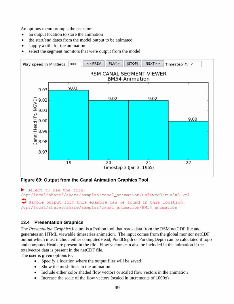
An options menu prompts the user for: • an output location to store the animation • the start/end dates from the model output to be animated • supply a title for the animation • select the segment monitors that were output from the model

Figure 69: Output from the Canal Animation Graphics Tool

Select to use the file: /opt/local/share3/share/samples/canal_animation/BM54wcd3/run3x3.xml

Sample output form this example can be found in this location: /opt/local/share3/share/samples/canal_animation/BM54_animation

13.4 Presentation Graphics The Presentation Graphics feature is a Python tool that reads data from the RSM netCDF file and generates an HTML viewable timeseries animation. The input comes from the global monitor netCDF output which must include either computedHead, PondDepth or PondingDepth can be calculated if topo and computedHead are present in the file. Flow vectors can also be included in the animation if the totalvector data is present in the netCDF file. The user is given options to:

• Specify a location where the output files will be saved • Show the mesh lines in the animation • Include either color shaded flow vectors or scaled flow vectors in the animation • Increase the scale of the flow vectors (scaled in increments of 1000x)

99

• Specify the size of a square grid (25x25 is default) that is used to acquire the mesh cells that will provide the flow vector values in the animation

• Specify a colorflood min/max range for assigning 20 bracketed color ranges to the shaded cells in the animation

• Specify the variable to be animated (computedhead, ponddepth or pondingdepth which is a calculation using (topo-computedhead)

• Specify the method for acquiring the timesteps to be animated. Either a timestep increment (5 = every 5th timestep) or day of the month (31=last day of every month)

• Select a color ramp • Select the start/end timestep from the netCDF model output file

Figure 70: Presentation Graphics Tool Menu Output from the Presentation Graphics Tool is in the form of an HTML browser viewable animation. Each individual timestep is saved in PNG format and can be viewed in the output directory that was specified when the animation was created. The animation viewer has controls to: stop, start, go backup,

100

go forward. The display includes: a color legend, the timestep being viewed and meta information documenting the units, file name and variable being displayed.

Select to view the file: /opt/local/share3/share/samples/C111/CERP_Alts/output/SR5_sss/C111_PIR1_Alt2Db.nc

Specify an output directory where you would like to store the output Click the None option for flow vectors Select a colorflood min/max of 0 to 4 Select the ComputedHead data type Select a timestep increment of 1 Select color ramp 3 Select timestep 0 as the start and timestep 14 as the end timestep Click the Generate button to create the animation

Figure 71: Output from the Presentation Graphics Tool

101

13.5 Verification Plots The Verification Plot feature is a Python tool that generates a series of three hydrographs showing comparison stages for RSM model output, SFWMM model output and Historical data. The hydrographs are formatted to show data for three specific ranges: 1984-1995, 1981-1983, 1996-2000. The output also includes statistics comparing the RSM and SFWMM output. The tool reads in an ASCII CONTROL FILE that contains references to data locations. An options menu also offers a choice to turn the display of the statistics on/off and to input a title for the Graph. CONTROL FILE: file ./output/glades_lecsa_output.dss ./output/struct_flow.dss ./output/struct_flow.dss run CH_EVER1 /GLADES_LECSA/EVER1/STAGE//1DAY/SIMULATED/ /SFRSM/S2/STAGE//1DAY/CALC/ /SFRSM/S3/STAGE//1DAY/CALC/

Select to view the file: /opt/local/share3/share/samples/verification_plots/sample.ctl

Specify a title for the plot Specify to show statistics Click the Generate button to create the Verification Plots.

102

Figure 72: Output from the Verification Tool

13.6 Inundation Report The Inundation Report feature is a Python tool that produces two graphs: 1) Ponding Stage Hydrograph 2) Stage Distribution Curve. The distribution curve shows the percent of time depth exceeds the ground elevation and an optional offset line. This tool uses three input files: NetCDF FILE: expected to contain Topography and ComputedHead to calculate PondDepth Cell ID CSV FILE: Cell ID, Landuse, Index, Eval Area, Offset Area1, 1, 1, 512, 1,-0.65 Area1, 1, , 512, 1, -0.65 LANDUSE CSV FILE:

LUCode, PDLD#, LU, Hydroperiod Range(mths), Seasonal Wet Level(ft), Seasonal Dry Level(ft), Temp

410,4.1, Cypress Swamp, 6 - 8,1.5,-1.5, junk 420,4.2, Hardwood Swamp, 8 - 10, 2, -1, junk

103

An options menu provides a method to:

• Specify a start/end date • Specify a daily or a weekly time period • Set date ranges for wet year, avg year and dry year

Figure 73: Inundation Report Tool Options Menu

Select to view the file: /opt/local/share3/share/samples/inundation_report/calib.nc, Multi_obs_cells_sample.csv, and landuse_v2_3b.csv

Specify a start/end date Select a Daily time period Accept the default date ranges Click the Generate button to create the inundation report

104

Figure 74: Output from the Inundation Report Tool

13.7 Levee Seepage Report The Levee Seepage Report feature is a Python tool that generates flow graphs showing seepage across a levee. Three graphs are produced for each levee: marsh-to-drycell, marsh-to-segment, drycell-to-segment. A report can also be produced showing daily, monthly or annual summarization of the data. As input this tool function against DSS or wbbudget NC files, and it requires a corresponding levee-seepage XML file from the model run. Optionally it can accept one or more than one XML files.

Required Data files • wbbudgetpackage NC or DSS file • XML file: levee-seepage.xml

Sample output form this example can be found in this location: /opt/local/share3/share/samples/leveeseepage_report/levee_seepage.pdf Examples of the XML files can be found in Appendix G. An options menu provides a method to select the input files, specify a start/end date. The tool acquires the levees and produces a list of seepage locations to choose from.

105

Select to use the files: /opt/local/share3/share/samples/leveeseepage_report/wbbudget.nc and single-seep.xml

Accept the default start date Select one or several seepage(s) across a levee. Indicate if you want a CSV report Indicate if Click the generate button to create the Levee Seepage report.

Figure 75: Levee Seepage Report Options Menu

106

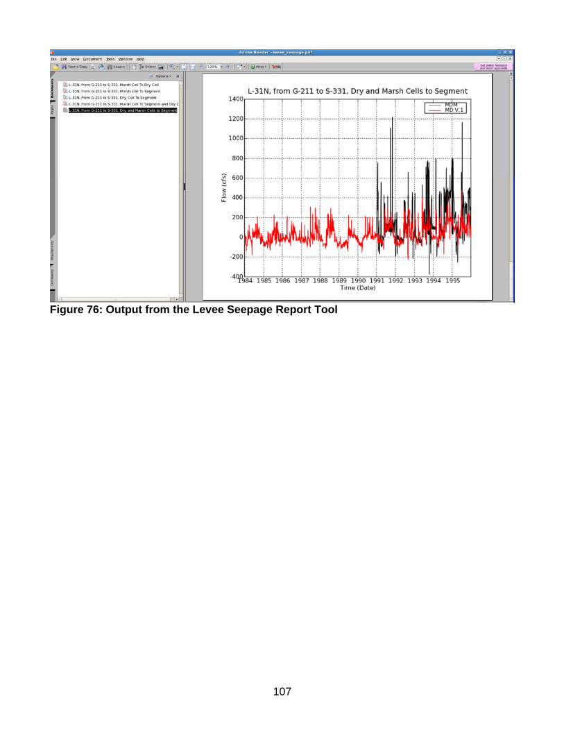
Figure 76: Output from the Levee Seepage Report Tool

107

Chapter 14

Performance Measure Graphics

Figure 77: Performance Measure Graphics Menu The RSM GUI offers a variety of Performance Measure Graphic (PMG) and Performance Measure Indicator (PMI) options. These tools have been designed to meet the needs for the Northern Everglades Project but they may be applied and adopted to fit other projects.

Some of the PMG and PMI tools use SOURCE FILES as input. These are ASCII text files designed to contain references to data files, titles and other formatting information that help control the specific application being run. Source files are carried over from previous usage on the SFWMM model performance measure graphics. The HELP button on each RSM GUI tools that use source files contains a reference where a sample source file can be found. Where it is helpful, these instructions reference how to create each source file. Source File An example source file can be found in Appendix F. The file species the location for each dataset, text for the legend, text for the main title, and other formatting controls used by the XMGRACE application used to produce the graphics.

108

14.1 LOK PMG’s The LOK PMG’s menu includes a list of tools to produce Lake Okeechobee Performance Measure Graphics for the Northern Everglades Project.

14.1.1 LOK Envelope PMG This tool generates 4 PMG’s: LOK Envelope (Above, Below, Extreme High, Extreme Low). Output is generated in PDF format. The command line option to run this tool outputs files into a Lok sub-directory from where the tool is run. Output files are given default names:

Figure 78: lo1_weekly_low_lake_annualized.pdf

109

Figure 79: lo2_weekly_high_lake_annualized.pdf

Figure 80: lo3_weekly_low_annualized.pdf

110

Figure 81: lo3_weekly_high_lake_annualized.pdf Command Line:

• source the source_pmg1.txt source file. • execute: /opt/local/share3/bin/run_lo_generator.scr • Output: stored in Lok sub-directory

TOOLBAR:

• From RSMTOOLBAR select menu choice OUTPUT GRAPHICS>>LOK PMGs>>1-4 LOK Envelope

• Provide location of source_file • Output: 4 PDF files are displayed on screen.

Sample Files: /opt/local/share3/share/samples/pmg_input/source_pmg1.txt

111

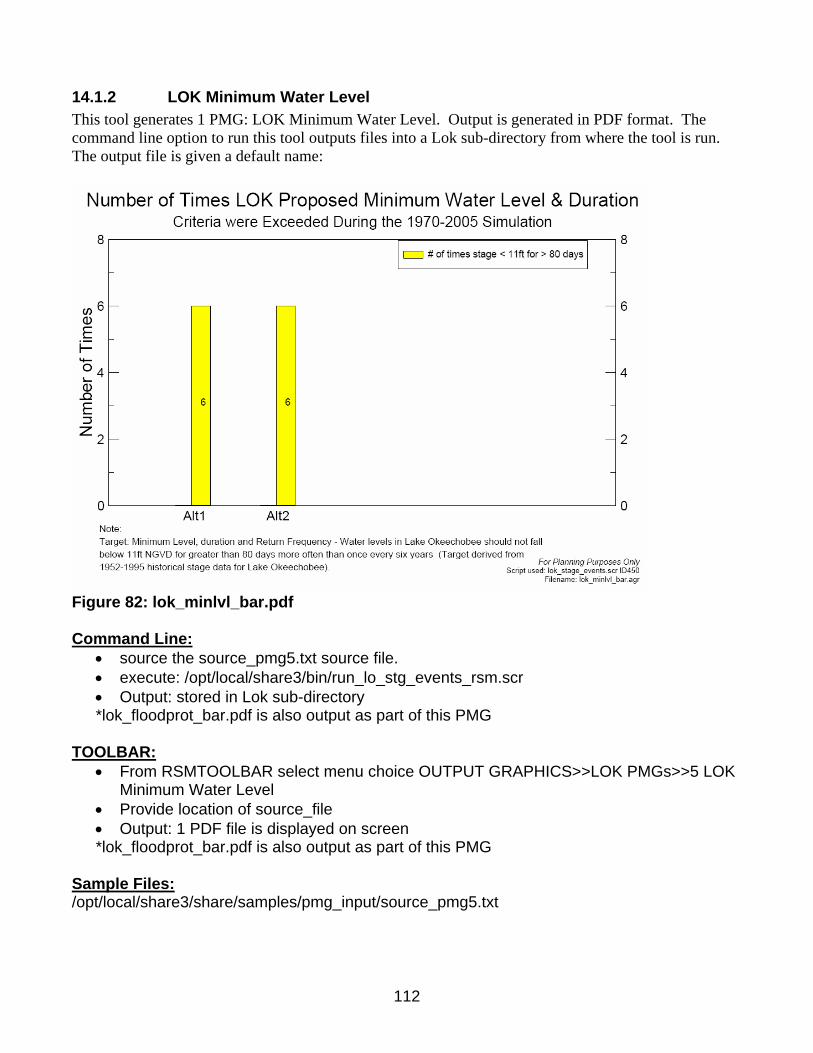
14.1.2 LOK Minimum Water Level This tool generates 1 PMG: LOK Minimum Water Level. Output is generated in PDF format. The command line option to run this tool outputs files into a Lok sub-directory from where the tool is run. The output file is given a default name:

Figure 82: lok_minlvl_bar.pdf Command Line:

• source the source_pmg5.txt source file. • execute: /opt/local/share3/bin/run_lo_stg_events_rsm.scr • Output: stored in Lok sub-directory *lok_floodprot_bar.pdf is also output as part of this PMG

TOOLBAR:

• From RSMTOOLBAR select menu choice OUTPUT GRAPHICS>>LOK PMGs>>5 LOK Minimum Water Level

• Provide location of source_file • Output: 1 PDF file is displayed on screen *lok_floodprot_bar.pdf is also output as part of this PMG

Sample Files: /opt/local/share3/share/samples/pmg_input/source_pmg5.txt

112

14.2 Estuary PMG’s The Estuary PMG’s menu includes a list of tools to produce St. Lucie and Caloosahatchee Estuary Performance Measure Graphics for the Northern Everglades Project.

14.2.1 Caloo and STL This tool generates 4 PMG’s: High Discharge and Salinity Envelope Criteria for St. Lucie Estuary and Caloosahatchee Estuary. Output is generated in PDF format. The command line option to run this tool outputs files into a Estuary sub-directory from where the tool is run. The output files are given a default names:

Figure 83: caloos_2800_4500_flow_bar.pdf

113

Figure 84: caloos_salinity_flow_bar.pdf

Figure 85: stluc_2000_flow_bar.pdf

114

Figure 86: stluc_salinity_flow_bar.pdf Command Line:

• source the source_pmg6.txt source file. • execute: /opt/local/share3/bin/run_estuary_rsm.scr • Output: stored in Estuary sub-directory

TOOLBAR:

• From RSMTOOLBAR select menu choice OUTPUT GRAPHICS>>Estuary PMGs>>1-4 Caloo and STL

• Provide location of source_file • Output: 4 PDF’s are displayed on screen.

Sample Files: /opt/local/share3/samples/pmg_input/source_pmg6.txt

115

14.2.2 Caloo and STL (NERSM rivers) This tool is a modification from the original Caloo STL PMG tool. The target values have been changed for STL High Discharge Criteria(21 & 6), the minimum <350cfs has been deleted from the STL Salinity graph and the STL Salinity graph reflects mean monthly values instead of a 14-day moving average. This tool generates 4 PMG’s: High Discharge and Salinity Envelope Criteria for St. Lucie Estuary and Caloosahatchee Estuary. Output is generated in PDF format. The command line option to run this tool outputs files onto the screen where they can be saved to any location by the user. The output files are given default names but they can be changed as they are being saved by the user:

Figure 87: caloos_nersm_2800_4500_flow_bar.pdf

116

Figure 88: caloos_nersm_salinity_flow_bar.pdf

Figure 89: stluc_nersm_2000_flow_bar.pdf

117

Figure 90: stluc_nersm_salinity_flow_bar.pdf Command Line:

• execute: /opt/local/share3/bin/PMG-CALOOSTL-NERSM [yourcontrolfile.ctl] • Output: displayed on screen

TOOLBAR:

• From RSMTOOLBAR select menu choice OUTPUT GRAPHICS>>Estuary PMGs>>1-4 Caloo and STL (NERSM rivers)

• Provide location of source_file • Output: 4 PDF’s are displayed on screen.

Sample Files: /opt/local/share3/samples/pmg_input/source_pmg6.txt

118

14.2.3 C43 Target Flow Index This tool generates one graphic that compares a pre-selected target flow against alternative flows. Output is generated in PDF format. There is no command line option to run this tool as of yet.

Figure 91: C43 Target Flow Index PMG Command Line:

• execute: /opt/local/share3/bin/PMG_TFI [yourcontrolfile.ctl] • Output: displayed on screen

TOOLBAR:

• From RSMTOOLBAR select menu choice OUTPUT GRAPHICS>>Estuary PMGs>> >>C43 Target Flow Index

• Provide location of control_file • Output: 1 PDF is displayed on screen.

Sample Files: /opt/local/share3/samples/pmg_input/source_tfi.ctl

119

14.3 KISS PMG’s The KISS PMG’s menu includes a list of tools to produce Kissimmee River Performance Measure Graphics for the Northern Everglades Project.

14.3.1 LKB Mean Monthly Flows This tool generates one PMG: LKB Mean Monthly Flows. Output is generated in PDF format. Output is generated to the screen and can be saved to any specified location.

Figure 92: kiss-pmg1.pdf LKB Mean Monthly Flows Command Line:

• execute: on whqoom01d • /opt/loca/share3/bin/kiss-pmg1 [control file name]

TOOLBAR: • From RSMTOOLBAR select menu choice OUTPUT GRAPHICS>>KISS PMGs>>1 LKB

Mean Monthly Flows • Provide location of control_file • Output: PDF is displayed on screen along with the XMGRACE (.agr) file used to

generate the graphic. Sample Files: /opt/local/share3/samples/pmg_input/kiss-pmg1.ctl

120

14.3.2 LKB Seasonal Min/Max Flows This tool generates 4 PMG’s: LKB Seasonal Min and Seasonal Max Flows for S-65 and S-65E. Output is generated into one indexed PDF file. Output is generated to the screen and can be saved to any specified location.

Figure 93: kiss-pmg2.pdf maximum monthly flows at S-65

Figure 94: kiss-pmg2.pdf minimum monthly flows at S-65

121

Figure 95: kiss-pmg2.pdf maximum monthly flows at S-65E

Figure 96: kiss-pmg2.pdf minimum monthly flow at S-65E

122

Command Line: • execute: from whqoom01d • /opt/local/share3/bin/kiss-pmg2 [control file name]

TOOLBAR: • From RSMTOOLBAR select menu choice OUTPUT GRAPHICS>>KISS PMGs>>2 LKB

Seasonal Min/Max Flows • Provide location of control_file • Output: PDF is displayed on screen along with ASCII files containing data used to

generate the graphs. Sample Files: /opt/local/share3/samples/pmg_input/kiss-pmg2.ctl

14.3.3 LKB 14 Day Low Flows This tool generates 2 PMG: LKB 14 Day Low Flows for S-65 and S-65E. Output is generated into one indexed PDF file. Output is generated to the screen and can be saved to any specified location.

Figure 97: kiss-pmg3.pdf Flows at S-65

123

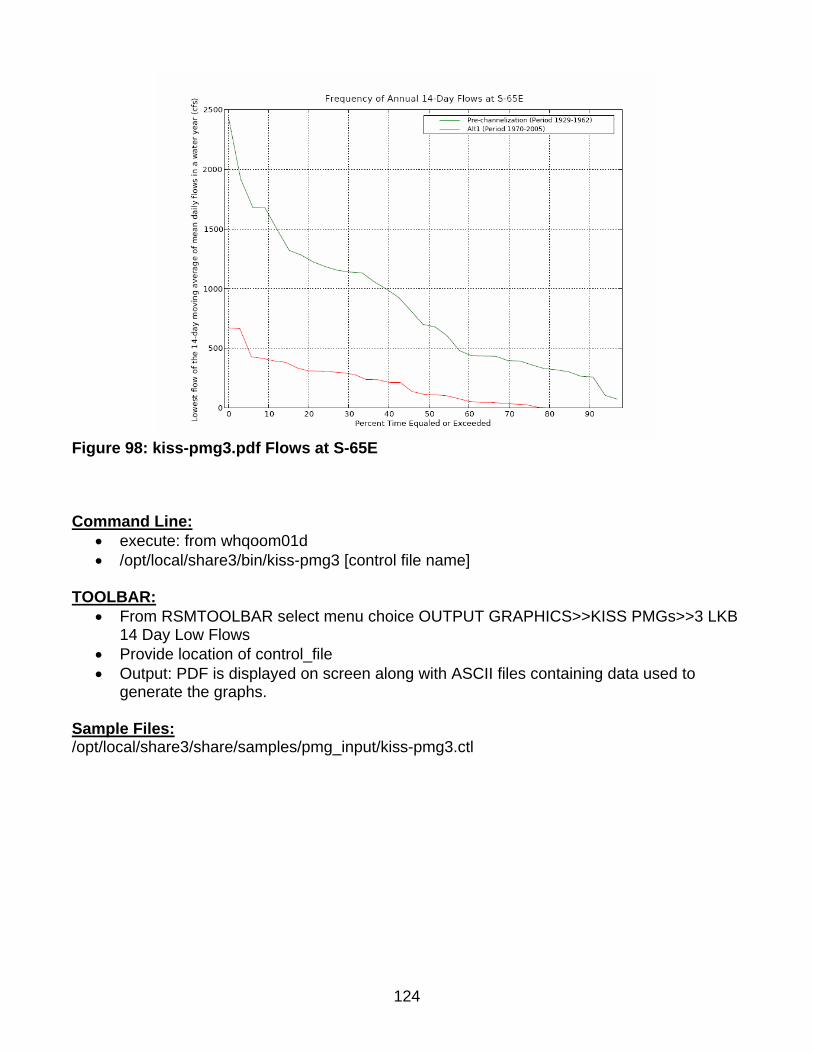
Figure 98: kiss-pmg3.pdf Flows at S-65E Command Line:

• execute: from whqoom01d • /opt/local/share3/bin/kiss-pmg3 [control file name]

TOOLBAR: • From RSMTOOLBAR select menu choice OUTPUT GRAPHICS>>KISS PMGs>>3 LKB

14 Day Low Flows • Provide location of control_file • Output: PDF is displayed on screen along with ASCII files containing data used to

generate the graphs. Sample Files: /opt/local/share3/share/samples/pmg_input/kiss-pmg3.ctl

124

14.3.4 KUB Probable High Lake Stages This GUI tool generates 1 PMG and 3 HTML tables: KUB probable High Lake Stages, Duration Above High Pool Stage, High Stage Summary, and Peak Annual Stage. Users can specify the date range for running this tool. Output is generated in PDF format and HTML. Output is generated to the screen and can be saved to any specified location.

Figure 99: kiss-pmg4.pdf

125

<partial view>

126

<partial view>

Figure 100: kiss-pmg4.html Command Line:

• execute: from whqoom01d • /opt/local/share3/bin/kiss-pmg4 [control file name]

TOOLBAR: • From RSMTOOLBAR select menu choice OUTPUT GRAPHICS>>KISS PMGs>>4 KUB

Probable High Lake Stages • Provide location of control_file • Output: 1 PDF is displayed on screen along with a browser window displaying 3 tables.

Sample Files: /opt/local/hsare3/share/samples/pmg_input/kiss-pmg4.ctl

127

14.4 PMI’s The PMI’s menu includes a list of tools to produce Performance Measure indicators for the Northern Everglades Project.

14.4.1 LOK Stage Duration Curve This tool generates 1 PMG: LOK Stage Duration Curve. Output is generated in PDF format. Output is generated to the screen and can be saved to any specified location.

Figure 101: pmi1.pdf Command Line:

• execute: from whqoom01d • /opt/local/share3/bin/pmi-1 [control file name]

TOOLBAR:

• From RSMTOOLBAR select menu choice OUTPUT GRAPHICS>>LOK PMIs>>2 LOK Stage Duration Curve

• Provide location of control_file • Output: 1 PDF file is displayed on screen.

Sample Files: /opt/local/share3/share/samples/pmg_input/pmg_pmi/pmi1.ctl

128

14.4.2 Water Supply Indicator 7 Worst Years This tool generates 1 PMG: Water Supply Indicator 7 Worst Years. The command line option to run this tool outputs files into a Wsupply sub-directory from where the tool is run. The output file is given a default name:

Figure 102: losa_cutback_yrs_bar.pdf Command Line:

• source the source_pmi5a.txt source file. • execute: /opt/local/share3/bin/run_losa_cutback_yrs.scr • Output: stored in Wsupply sub-directory

TOOLBAR:

• From RSMTOOLBAR select menu choice OUTPUT GRAPHICS>>PMI’s>>5a Watersupply indicator

• Provide location of source_file • Output: 1 PDF file is displayed on screen.

Sample Files: /opt/local/share3/share/samples/pmg_input/source_pmi5a.txt NOTE: The only change necessary to make in the source file for this PMI is the line indicating the location of the data.txt file. The data.txt file contains the data for creating the graph. See a sample data.txt file at: /opt/local/share3/share/samples/pmg_input/data/pmi5a.txt

129

14.4.3 4-1in-1 LOK Water Supply Indicator This tool generates 1 PMG: Water Supply Indicator 7 Worst Years. The command line option to run this tool outputs files into a Wsupply sub-directory from where the tool is run. The output file is given a default name:

Figure 103: losa_dmd_4in1.pdf Command Line:

• source the source_pmi5b.txt source file. • execute: /opt/local/share3/bin/run_4in1_data_rsm.scr • Output: stored in Wsupply sub-directory

TOOLBAR:

• From RSMTOOLBAR select menu choice OUTPUT GRAPHICS>>PMI’s>>5b 4-in-1 LOK Water Supply Indicator

• Provide location of source_file • Output: 1 PDF file is displayed on screen.

Sample Files: /opt/local/share3/share/samples/pmg_input/source_pmi5b.txt NOTE: The only change necessary to make in the source file for this PMI is the line indicating the location of the data.txt file. The data.txt file contains the data for creating the graph. See a sample data.txt file at: /opt/local/share3/share/samples/pmg_input/data/pmi5b.txt

130

14.4.4 Intra-Annual Lake Variability This tool generates 1 HTML table: Intra-annual lake Variability. Output is generated in HTML format. Output is generated to the screen, is displayed in a browser and can be saved to any specified location.

Figure 104: pmi8.html Command Line:

• execute: from whqoom01d • /opt/local/share3/bin/pmi-8 [control file name]

TOOLBAR:

• From RSMTOOLBAR select menu choice OUTPUT GRAPHICS>>PMI’s>>8 Intra-annual Lake Variability

• Provide location of control_file • Output: 1 HTML file is displayed on screen.

Sample Files: /opt/local/share3/share/samples/pmg_input/pmi8.ctl

131

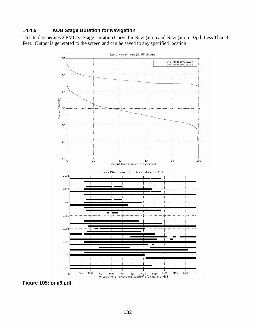
14.4.5 KUB Stage Duration for Navigation This tool generates 2 PMG’s: Stage Duration Curve for Navigation and Navigation Depth Less Than 3 Feet. Output is generated to the screen and can be saved to any specified location.

Figure 105: pmi9.pdf

132

Command Line: • execute: from whqoom01d • /opt/local/share3/bin/pmi-9 [control file name]

TOOLBAR:

• From RSMTOOLBAR select menu choice OUTPUT GRAPHICS>>PMI’s>>9 KUB Stage Duration for Navigation

• Provide location of control_file • Output: 1 PDF file is displayed on screen along with the data files used to produce the

graphs. Sample Files: /opt/local/share3/share/samples/pmg_input/pmi9.ctl

133

Chapter 15

Cluster Tools Menu

Figure 106: Cluster Tools Menu

15.1 Top Processes The Top Processes feature is a Linux System Call to the “top” command. Top displays list of the top 10 processes utilizing the CPU on the computer on which the RSM GUI is currently being run from. An HSE process represents an executing RSM model run.

Figure 107: Display produced by the "Top" Command

15.2 Load The Load feature is a Linux System Call to the “load” command. Load displays a moving bar graph representing the CPU load on the server on which the RSM GUI is currently being run from.

Figure 108: Display produced by the "Load" Command

134

15.3 Cluster Report The Cluster Report feature is a browser link to Ganglia. Ganglia is a scalable distributed monitoring system for high-performance computing systems such as clusters and Grids. http://ganglia.sourceforge.net/

135

Chapter 16

HELP Menu

Figure 109: Help Menu

16.1 About… The About feature displays the version and release date of the RSM GUI.

16.2 Request Help The Request Help feature provides a means to report problems directly to the RSM GUI Development Team. The user can enter a message which is then emailed to the development team.

16.3 RSM Homepage The RSM Homepage feature is a link to the RSM Homepage. Information regarding the RSM development, RSM implementations and the RSM GUI is posted to the RSM Homepage.

136

Figure 110: RSM Homepage

16.4 RSM GUI UserGuide The RSM GUI UserGuide feature is a link to the current RSM GUI Users Guide. It is a PDF document containing instructions on the use of every tool in the RSM GUI.

137

16.5 SFRSM Toolbar Python Documentation

16.6 CVS/SVN Code Repository The CVS/SVN feature is a browser link to SVN Subversion. SVN is a software version control system. The RSM SVN repository contains the versioned RSM HSE model code and RSM GUI code. http://subversion.tigris.org/

138

16.7 Bugzilla 2.22 The Bugzilla 2.22 feature is a link to the browser based Bugzilla work task management system. Bugzilla is used to track all RSM tasks and projects.

16.8 fixDSS The fixDSS feature is a Python tool that reads in an RSM DSS file and generates a duplicate file with corrected time/date stamps. In earlier version of the RSM (prior to 1.1.1) the DSS output files periodically contained a data format that was not readable by Python 2.4. This tool has been included as a precaution in case older files are still in use.

If a tool encounters an error when reading a DSS file and generates an error message referring to “zrt” or “not a regular timeseries” then fxDSS is needed to correct the problem.

16.9 Customize Toolbar The Customize Toolbar feature is an option to select customized views of the RSM GUI Toolbar. The options and dropdown menus offered on the RSM GUI are driven by an XML. The Default XML is what most users will use when the run the RSM GUI. Advanced users may prefer to select from a list of customized views or they may choose to create their own XML. This feature will be further developed and automated in future versions of the RSM GUI.

Figure 111: RSM GUI Customized Toolbar

139

Appendix A - Definitions, Abbreviations and Acronyms Definitions Term Definition calibration XML The main XML used to configure an RSM scenario. model run XML The main XML used to configure an RSM scenario. configuration XML The main XML used to configure an RSM scenario. Citrix Commercial computer application access platform. GMS Environmental Modeling Systems Inc. groundwater

modeling and mesh creation software Linux Open source, UNIX like operating system. geodatabase a database designed to store query, and manipulate

geographic information and spatial data. DSS HEC Data Storage System file format used for storing

time series data polygon A finite number of sequential line segments which

begin and end at the same, point forming a closed planar path.

Abbreviations & Acronyms Abbreviation Meaning ESRI Environmental Systems Research Institute ET Evapotranspiration GIS Geographic Information System GUI Graphical User Interface HESM Hydrologic and Environmental Simulation Modeling HIS Habitat Suitability Index HPM Hydrologic Processing Module in the RSM HSE Hydrologic Simulation Engine in the RSM HTML Hypertext Markup Language IR Indicator Region KISS Kissimmee KUB Kissimmee Upper Basin LKB Lake Kissimmee Basin LOK Lake Okeechobee MFL Minimum Flows and Levels MSE Management Simulation Engine in the RSM netCDF Network Common Data Format NSRSM Natural Systems Regional Simulation Model PMG Performance Measure Graphic PMI Performance Measure Indicator PMViewer Performance Measure Graphics Viewer PWS Public Water Supply RSM Regional Simulation Model SFWMD South Florida Water Management District

140

STA Stormwater Treatment Area SWMM South Florida Water Management Model XML Extensible Markup Language

141

Appendix B – RSM Template Geodatabase Report

Geodatabase Reporting Tool

Date Of Report 6/8/2005 4:47:17 PM Generated By jsulliva (on 7J0YF61) Geodatabase Type Personal [Version 1.3.0 (Previous Release)] Database \\dcluster1\oom\sfrsm\data\gis\network\sumit\sfrsm_gis_v4_copy.mdb

Geodatabase Report Contents Geodatabase Summary

Geometric Network Summary

ObjectClass Information

RelationshipClass Information

Domain Information

Spatial Reference Information

Row/Feature Count Information

Geodatabase Summary FeatureDataset Object Name (Alias) Type Geometry Subtypes

broward_subset (broward_subset) (C) Simple Feature Polyline None canal_has_mse_unit RelationshipClass canal->mse_unit

canal (canal) (C) Complex Edge Polyline Canal Water Mover

mesh_bnd (mesh_bnd) (C) Simple Feature Polygon None mesh_framework (mesh_framework) (C) Simple Edge Polyline None mesh_node (mesh_node) (C) Simple Junction Point None mesh_pnt (mesh_pnt) (C) Simple Feature Point None mesh (mesh) (C) Simple Feature Polygon None sfrsm_gis_Net_Junctions (sfrsm_gis_Net_Junctions) (C) Simple Junction Point None sfrsm_gis_Net GeometricNetwork sfrsm_gis_Net2_Junctions (sfrsm_gis_Net2_Junctions) (C) Simple Junction Point None sfrsm_gis_Net2 GeometricNetwork structure_has_culvert_box RelationshipClass structure->culvert_box

RelationshipClass structure->culvert_circularstructure_has_culvert_circular

RelationshipClass structure->fixed_weirstructure_has_fixed_weir

RelationshipClass structure->genstrucstructure_has_genstruc

RelationshipClass structure->mse_unitstructure_has_mse_unit

RelationshipClass structure->pumpstructure_has_pump

RelationshipClass structure->spillwaystructure_has_spillway

RelationshipClass structure->variable_weirstructure_has_variable_weir

structure (structure) (C) Simple Junction Point Diversion Structure Inline Structure Junction Block

sfrsm_gis (S)

watersheds (watersheds) (C) Simple Feature Polygon None culvert_box (culvert_box) (C) Table None None culvert_circular (culvert_circular) (C) Table None None fixed_weir (fixed_weir) (C) Table None None genstruc (genstruc) (C) Table None None

None

mse_const (mse_const) (C) Table None None

142

mse_dss (mse_dss) (C) Table None None mse_inout (mse_inout) (C) Table None None mse_node (mse_node) (C) Table None None mse_rc (mse_rc) (C) Table None None mse_unit (mse_unit) (C) Table None None pump (pump) (C) Table None None spillway (spillway) (C) Table None None variable_weir (variable_weir) (C) Table None None boundary Domain Coded Value EnabledDomain Domain Coded Value rc_domain Domain Range vaule Domain Coded Value WM_type Domain Coded Value

Geometric Network Summary Geometric Newtork Name Role FeatureClass Name Links

sfrsm_gis_Net_Junctions Simple Junction structure

Complex Junction None Simple Edge None

sfrsm_gis_Net

Complex Edge canal EJ Rules EE Rules

mesh_node Simple Junction sfrsm_gis_Net2_Junctions

Complex Junction None Simple Edge mesh_framework EJ Rules EE Rules

sfrsm_gis_Net2

Complex Edge None

ObjectClass Information broward_subset (Simple Feature) (Polyline) No Subtypes Field Name Field Type Pre Sc Len DV Domain OBJECTID OID 0 0 4 Shape Geome ry t 0 0 0 FNODE_ Integer 0 0 4 TNODE_ Integer 0 0 4 LPOLY_ Integer 0 0 4 RPOLY_ Integer 0 0 4 LENGTH Double 0 0 8 BRO_CANAL8 Integer 0 0 4 BRO_CANA_ 1 Intege r 0 0 4 DIST_CODE String 0 0 1 0 HYDR_CON D Double 0 0 8 BOT_THICK Double 0 0 8 CSLOPE Double 0 0 8 MAX_LAYER Double 0 0 8 CAN_NAME String 0 0 15 BOT_ELEV Double 0 0 8 TOP_WIDTH Double 0 0 8 BOT_WIDTH Double 0 0 8 SIDE_THICK Doubl e 0 0 8 STATUS String 0 0 1 0 FUNCTION String 0 0 5 OPT_LEV Double 0 0 8 ROAD_CROWN Double 0 0 8 SIDE_SLOPE Double 0 0 8 STRUCTURE String 0 0 15 CLASS String 0 0 1 LEVEL_ Double 0 0 8 MAXBOT_THK Double 0 0 8

143

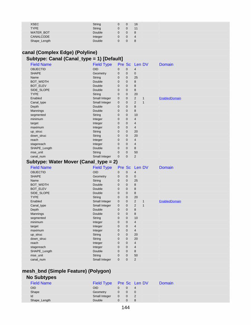
XSEC String 0 0 16 TYPE String 0 0 1 1 WATER_BOT Double 0 0 8 CANALCODE Integer 0 0 4 Shape_Length Double 0 0 8 canal (Complex Edge) (Polyline) Subtype: Canal (Canal_type = 1) [Default] Field Name Field Type Pre Sc Len DV Domain OBJECTID OID 0 0 4 SHAPE Geometry 0 0 0 Name String 0 0 25 BOT_WIDT H Double 0 0 8 BOT_ELEV Double 0 0 8 SIDE_ LOPE S Doubl e 0 0 8 TYPE String 0 0 20 Enabled Small Integer 0 0 2 1 EnabledDomain

Canal_type Small Integer 0 0 2 1 Depth Double 0 0 8 Mannings Double 0 0 8 segment ed String 0 0 1 0 minimum Integer 0 0 4 target Integer 0 0 4 maximum Integer 0 0 4 up_struc String 0 0 20 down_struc String 0 0 20 reach Integer 0 0 4 stagereach Integer 0 0 4 SHAPE_Length Doubl e 0 0 8 mse_unit String 0 0 5 0 canal_num Small Integer 0 0 2 Subtype: Water Mover (Canal_type = 2) Field Name Field Type Pre Sc Len DV Domain OBJECTID OID 0 0 4 SHAPE Geometry 0 0 0 Name String 0 0 2 5 BOT_WIDT H Double 0 0 8 BOT_ELEV Double 0 0 8 SIDE_ LOPE S Doubl e 0 0 8 TYPE String 0 0 20 Enabled Small Integer 0 0 2 1 EnabledDomain

Canal_type Small Integer 0 0 2 1 Depth Double 0 0 8 Mannings Doubl e 0 0 8 segment ed String 0 0 1 0 minimum Integer 0 0 4 target Integer 0 0 4 maximum Integer 0 0 4 up_struc String 0 0 20 down_struc String 0 0 20 reach Integer 0 0 4 stagereach Integer 0 0 4 SHAPE_Length Doubl e 0 0 8 mse_unit String 0 0 5 0 canal_num Small Integer 0 0 2 mesh_bnd (Simple Feature) (Polygon) No Subtypes Field Name Field Type Pre Sc Len DV Domain OID OID 0 0 4 Shape Geometry 0 0 0 Id Small Integer 0 0 2 Shape_Length Double 0 0 8

144

Shape_Area Double 0 0 8 mesh_framework (Simple Edge) (Polyline) No Subtypes Field Name Field Type Pre Sc Len DV Domain OBJECTID_12 OID 0 0 4 Shape Geome try 0 0 0 DENSITY Double 0 0 8 LINEID Double 0 0 8 DSCRPN String 0 0 30 Enabled Small Integer 0 0 2 1 EnabledDomain

checked String 0 0 5 noflow String 0 0 5 0 Shape_Length Doubl e 0 0 8 boundary String 0 0 50 boundary

mesh_node (Simple Junction) (Point) No Subtypes Field Name Field Type Pre Sc Len DV Domain OID OID 0 0 4 Shape Geometry 0 0 0 Id Small Integer 0 0 2 X_coord Double 0 0 8 Y_coord Double 0 0 8 Z_coord Double 0 0 8 Enabled Small Integer 0 0 2 1 EnabledDomain

mesh_pnt (Simple Feature) (Point) No Subtypes Field Name Field Type Pre Sc Len DV Domain OID OID 0 0 4 S ape h Geometry 0 0 0 Id Small I teger n 0 0 2 X_coord Double 0 0 8 Y_coord Double 0 0 8 mesh (Simple Feature) (Polygon) No Subtypes Field Name Field Type Pre Sc Len DV Domain OID OID 0 0 4 Shape Geometry 0 0 0 Node1 Small Integer 0 0 2 Node2 Small Integer 0 0 2 Node3 Small Integer 0 0 2 lu88_flucs String 0 0 8 lu95_flucs String 0 0 4 topo Double 0 0 8 elev_bot_lyr1 Double 0 0 8 kh_lyr1 Double 0 0 8 lu88_beta String 0 0 10 lu95_beta String 0 0 10 bc_lko Small Integer 0 0 2 bc_tide Small Integer 0 0 2 Calib_reg String 0 0 100 topo2 Double 0 0 8 cellid Small Integer 0 0 2 meshid String 0 0 20 water String 0 0 50 county String 0 0 32 Shape_Length Double 0 0 8

145

Shape_Area Double 0 0 8 sfrsm_gis_Net_Junctions (Simple Junction) (Point) No Subtypes Field Name Field Type Pre Sc Len DV Domain OBJECTID OID 0 0 4 SHAPE Geometry 0 0 0 Enabled Small Integer 0 0 2 1 EnabledDomain

sfrsm_gis_Net2_Junctions (Simple Junction) (Point) No Subtypes Field Name Field Type Pre Sc Len DV Domain OBJECTID OID 0 0 4 SHAPE Geometry 0 0 0 Enabled Small Integer 0 0 2 1 EnabledDomain

structure (Simple Junction) (Point) Subtype: Inline Structure (Flow = 0) Field Name Field Type Pre Sc Len DV Domain OBJECTID OID 0 0 4 Shape Geometry 0 0 0 AREA Double 0 0 8 PERIMETER Double 0 0 8 IMFDCSTR_ Integer 0 0 4 IMFDCSTR_ID Intege r 0 0 4 NAME String 0 0 12 FLOW_TYPE String 0 0 15 CONTROL String 0 0 15 MATERIAL String 0 0 25 PURPOSE String 0 0 20 ESTUARY String 0 0 2 5 SOURCE String 0 0 4 GPSDEVICE String 0 0 20 FIELDSTA String 0 0 17 CANAL String 0 0 30 SYMBOL Integer 0 0 4 SYMBOL500K Integer 0 0 4 ANGLE Small Integer 0 0 2 VER IED IF String 0 0 3 STA String 0 0 5 NAME2 String 0 0 1 2 FLAG Small Integer 0 0 2 TIME_STAMP String 0 0 30 WALLMAP String 0 0 3 SYMBOLXWEB Integer 0 0 4 SYMBOLXWEB500K Integer 0 0 4 CRITICAL String 0 0 4 ANGLEM P A Small Integer 0 0 2 COUNTY String 0 0 12 OWNERSHIP String 0 0 10 POLYGONID Integer 0 0 4 SCALE Double 0 0 8 ANGLE_1 Integer 0 0 4 checked String 0 0 5 no SFWMM_i pose m String 0 0 10 struc type _ String 0 0 40 type String 0 0 1 0 Enabled Small Integer 0 0 2 1 EnabledDomain

Flow Small Integer 0 0 2 0 WM_type String 0 0 50 WM_type

Subtype: Diversion Structure (Flow = 1) [Default]

146

Field Name Field Type Pre Sc Len DV Domain OBJECTID OID 0 0 4 Shape Geometry 0 0 0 AREA Double 0 0 8 PERIMETER Double 0 0 8 IMFDCSTR_ Integer 0 0 4 IMFDCSTR_ID Integer 0 0 4 NAME String 0 0 12 FLOW_TY E P String 0 0 15 CONTROL String 0 0 15 MATERIAL String 0 0 25 PURPOSE String 0 0 20 ESTUARY String 0 0 25 SOURCE String 0 0 4 GPSDEVICE String 0 0 20 FIELDSTA String 0 0 17 CANAL String 0 0 3 0 SYMBOL Integer 0 0 4 SYMBO L500K Integer 0 0 4 ANGLE Small Integer 0 0 2 VERIFIED String 0 0 3 STA String 0 0 5 NAME2 String 0 0 12 FLAG Small Integer 0 0 2 TIME_STAMP String 0 0 3 0 WALLMAP String 0 0 3 SYMBOLXWEB Integer 0 0 4 SYMBOLXWEB500K Integer 0 0 4 CRITICAL String 0 0 4 ANGLEMAP Small Integer 0 0 2 COUNTY String 0 0 12 OWNERSHIP String 0 0 10 POLYGONID Integer 0 0 4 SCALE Double 0 0 8 ANGLE_ 1 Intege r 0 0 4 checked String 0 0 5 n o SFWMM_impose String 0 0 10 struc_type String 0 0 40 type String 0 0 10 Enabled Small Integer 0 0 2 1 EnabledDomain

Flow Small Integer 0 0 2 0 WM_type String 0 0 50 WM_type

Subtype: Junction Block (Flow = 2) Field Name Field Type Pre Sc Len DV Domain OBJECTID OID 0 0 4 Shape Geometry 0 0 0 AREA Double 0 0 8 PERIMETER Double 0 0 8 IMFDCSTR_ Integer 0 0 4 IMFDCSTR_ID Intege r 0 0 4 NAME String 0 0 12 FLOW_TYPE String 0 0 15 CONTROL String 0 0 15 MATERIAL String 0 0 25 PURPOSE String 0 0 20 ESTUARY String 0 0 25 SOURCE String 0 0 4 GPSDEVICE String 0 0 20 FIELDSTA String 0 0 17 CANAL String 0 0 30 SYMBOL Integer 0 0 4 SYMBOL500K Integer 0 0 4 ANGLE Small Integer 0 0 2 VERIFIED String 0 0 3 STA String 0 0 5 NAME2 String 0 0 12

147

FLAG Small Integer 0 0 2 TIME_STAMP String 0 0 3 0 WALLMAP String 0 0 3 SYMBOLXWEB Integer 0 0 4 SYMBOLXWEB500K Integer 0 0 4 CRITICAL String 0 0 4 ANGLEMAP Small Integer 0 0 2 COUNTY String 0 0 12 OWNERSHIP String 0 0 1 0 POLYGONID Integer 0 0 4 SCALE Double 0 0 8 ANGLE_1 Integer 0 0 4 checked String 0 0 5 no SFWMM_impose String 0 0 10 struc_type String 0 0 40 type String 0 0 1 0 Enab ed l Small Integer 0 0 2 1 E edDomainnabl

Flow Small Integer 0 0 2 0 WM_type String 0 0 50 WM_type

watersheds (Simple Feature) (Polygon) No Subtypes Field Name Field Type Pre Sc Len DV Domain OBJECTID_1 OID 0 0 4 Shape Geometry 0 0 0 OBJECTID Integer 0 0 4 Watershed String 0 0 50 SHAPE_Leng Double 0 0 8 extra Small I teger n 0 0 2 Shape_Leng th Double 0 0 8 Shape_Area Double 0 0 8 culvert_box [Table] No Subtypes Field Name Field Type Pre Sc Len DV Domain OBJECTID OID 0 0 4 structure_name String 0 0 255 station String 0 0 255 unitid String 0 0 255 eff_date Date 0 0 8 cul_length Integer 0 0 4 cul_heigh t Integer 0 0 4 cul_width Integer 0 0 4 ent_loss o c Integer 0 0 4 dis_coef Integer 0 0 4 cdw Integer 0 0 4 cdg Double 0 0 8 down_inv_el Integer 0 0 4 up_inv_el Integer 0 0 4 barrel_num Intege r 0 0 4 barrel_sha String 0 0 255 manning _co Intege r 0 0 4 con_type String 0 0 255 con_num Integer 0 0 4 gate_height Integer 0 0 4 gate_width Integer 0 0 4 hyd_rad Integer 0 0 4 area Integer 0 0 4 with_flow Integer 0 0 4 enabled Double 0 0 8 culvert_circular [Table]

148

No Subtypes Field Name Field Type Pre Sc Len DV Domain OBJECTID OID 0 0 4 structure_name String 0 0 255 dbhyd_sta String 0 0 255 unitid String 0 0 255 eff_dat e Date 0 0 8 cul_dia Integer 0 0 4 cul_length Integer 0 0 4 ent_loss o c Double 0 0 8 dis_coef Double 0 0 8 cdw Double 0 0 8 cdg Double 0 0 8 down_inv_el Double 0 0 8 up_inv_el Double 0 0 8 barrel_num Intege r 0 0 4 barrel_sha String 0 0 255 manning _co Doubl e 0 0 8 con_type String 0 0 255 con_num Integer 0 0 4 gate_dia Integer 0 0 4 gate_height Integer 0 0 4 gate_width Integer 0 0 4 hyd_rad Double 0 0 8 area Double 0 0 8 pipeopen Double 0 0 8 with_flow Integer 0 0 4 enabled Integer 0 0 4 fixed_weir [Table] No Subtypes Field Name Field Type Pre Sc Len DV Domain OBJECTID OID 0 0 4 structure_name String 0 0 255 station String 0 0 255 eff_date Integer 0 0 4 chan_w th id Integer 0 0 4 crest_el Double 0 0 8 crest_length Double 0 0 8 crest_width Double 0 0 8 notch_dept Double 0 0 8 top_width Double 0 0 8 dis_coef Double 0 0 8 with_flow Integer 0 0 4 enabl d e Doubl e 0 0 8 unitid String 0 0 50 genstruc [Table] No Subtypes Field Name Field Type Pre Sc Len DV Domain OBJE TID C OID 0 0 4 unitid String 0 0 255 dis_coef Double 0 0 8 with_flow Integer 0 0 4 enabled Integer 0 0 4 mse_const [Table] No Subtypes Field Name Field Type Pre Sc Len DV Domain OBJECTID OID 0 0 4 node_name String 0 0 50

149

unit_name String 0 0 5 0 const_supply Integer 0 0 4 const_supplyMax Integer 0 0 4 const_demand Integer 0 0 4 const_open Integer 0 0 4 const_close Integer 0 0 4 const_twheadLimit Integer 0 0 4 const_maintLeve l Integer 0 0 4 const_localLe el v Integer 0 0 4 const_fcLevel Integer 0 0 4 const_resLevel Integer 0 0 4 mse_dss [Table] No Subtypes Field Name Field Type Pre Sc Len DV Domain OBJECTID OID 0 0 4 node_name String 0 0 50 unit_name String 0 0 50 dss_supply String 0 0 50 dss_supplyMax String 0 0 50 dss_dema d n String 0 0 50 dss_open String 0 0 50 dss_close String 0 0 50 dss_twheadLimit String 0 0 50 dss_maintLevel String 0 0 50 dss_localLevel String 0 0 50 dss_fcLevel String 0 0 50 dss_resLevel String 0 0 50 mse_inout [Table] No Subtypes Field Name Field Type Pre Sc Len DV Domain OBJECTID OID 0 0 4 unit_name String 0 0 50 iostr c_name u String 0 0 50 type String 0 0 50 mse_node [Table] No Subtypes Field Name Field Type Pre Sc Len DV Domain OBJECTID OID 0 0 4 NODE_NAME String 0 0 11 PURPOSE String 0 0 11 LABEL String 0 0 10 DESIGN_CAP Double 0 0 8 MANAGED String 0 0 9 PN_OPEN String 0 0 33 PN_CLOS E String 0 0 3 3 wsPriorit y Small Integer 0 0 2 fcPriority Small Integer 0 0 2 DEMAND Small Integer 0 0 2 vaule

SUPPLY Small Integer 0 0 2 vaule

SUPPLYMAX Small Integer 0 0 2 vaule

OPEN_ Small Integer 0 0 2 vaule

CLOSE_ Small Integer 0 0 2 v ulea

twHeadLimit Small Integer 0 0 2 mse_rc [Table] No Subtypes Field Name Field Type Pre Sc Len DV Domain

150

OBJECTID OID 0 0 4 node_nam e String 0 0 50 unit_name String 0 0 50 rc_supply Integer 0 0 4 rc_supplyMax Integer 0 0 4 rc_demand Integer 0 0 4 rc_open Integer 0 0 4 rc_close Integer 0 0 4 rc_twheadLim it Integer 0 0 4 rc_maintLeve l Integer 0 0 4 rc_localLevel Integer 0 0 4 rc_fcLevel Integer 0 0 4 rc_resLevel Integer 0 0 4 mse_unit [Table] No Subtypes Field Name Field Type Pre Sc Len DV Domain OBJECTID OID 0 0 4 ID Integer 0 0 4 UNIT_NAME String 0 0 11 MAINT_LEVE Small Integer 0 0 2 vaule

LOCAL_LE E V Small Integer 0 0 2 vaule

FC_LEVEL Small Integer 0 0 2 vaule

RES_LEVEL Small Integer 0 0 2 vaule

pump [Table] No Subtypes Field Name Field Type Pre Sc Len DV Domain OBJECTID OID 0 0 4 structure_name String 0 0 255 case_ Integer 0 0 4 station String 0 0 255 unitid String 0 0 255 pum no p_ Integer 0 0 4 v_0 Double 0 0 8 v_0_2 5 Double 0 0 8 v_0_5 Double 0 0 8 v_0_75 Double 0 0 8 v_1 Double 0 0 8 v_1_25 Double 0 0 8 v_1_5 Double 0 0 8 v_1_75 Double 0 0 8 v_2 Double 0 0 8 v_2_2 5 Double 0 0 8 v_2_5 Double 0 0 8 v_2_75 Double 0 0 8 v_3 Double 0 0 8 v_3_25 Double 0 0 8 v_3_5 Double 0 0 8 v_3_75 Double 0 0 8 v_4 Double 0 0 8 v_4_2 5 Double 0 0 8 v_4_5 Double 0 0 8 v_4_75 Double 0 0 8 v_5 Double 0 0 8 v_5_25 Double 0 0 8 v_5_5 Double 0 0 8 v_5_75 Double 0 0 8 v_6 Double 0 0 8 v_6_2 5 Double 0 0 8 v_6_5 Double 0 0 8 v_6_75 Double 0 0 8 v_7 Double 0 0 8

151

v_7_2 5 Double 0 0 8 v_7_5 Double 0 0 8 v_7_75 Double 0 0 8 v_8 Double 0 0 8 v_8_25 Double 0 0 8 v_8_5 Double 0 0 8 v_8_75 Double 0 0 8 v_9 Double 0 0 8 v_9_2 5 Double 0 0 8 v_9_5 Double 0 0 8 v_9_75 Double 0 0 8 v_10 Double 0 0 8 v_10_25 Double 0 0 8 v_10_5 Double 0 0 8 v_10_75 Double 0 0 8 v_11 Double 0 0 8 v_11_2 5 Double 0 0 8 v_11_5 Double 0 0 8 v_11_75 Double 0 0 8 v_12 Double 0 0 8 v_12_25 Double 0 0 8 v_12_5 Double 0 0 8 v_12_75 Double 0 0 8 v_13 Double 0 0 8 v_13_2 5 Double 0 0 8 v_13_5 Double 0 0 8 v_13_75 Double 0 0 8 v_14 Double 0 0 8 v_14_25 Double 0 0 8 v_14_5 Double 0 0 8 v_14_75 Double 0 0 8 with_flow Integer 0 0 4 enabled Integer 0 0 4 spillway [Table] No Subtypes Field Name Field Type Pre Sc Len DV Domain OBJECTID OID 0 0 4 structure_ me na String 0 0 255 dbhyd_sta String 0 0 255 dis_coef Integer 0 0 4 with_flow Integer 0 0 4 enabled Double 0 0 8 unitid String 0 0 50 variable_weir [Table] No Subtypes Field Name Field Type Pre Sc Len DV Domain OBJECTID OID 0 0 4 structu e_name r String 0 0 255 station String 0 0 255 eff_date Integer 0 0 4 mincrest_el Double 0 0 8 maxcrest_el Double 0 0 8 crest_length Double 0 0 8 dis_coef Integer 0 0 4 with_flow Integer 0 0 4 enabl d e Doubl e 0 0 8 unitid String 0 0 50

RelationshipClass Information

152

Name canal_has_mse_unit [Simple] Cardinality One To Many Notification Both Attributed No Origin ObjectClass Destination ObjectClass Name canal [FeatureClass] mse_unit [Table] Key mse_unit [Origin Primary Key] UNIT_NAME [Origin Foreign Key] Labels mse_unit canal Rules This RelationshipClass has no rules. Name structure_has_culvert_box [Simple] Cardinality One To Many Notification None Attributed No Origin ObjectClass Destination ObjectClass Name structure [FeatureClass] culvert_box [Table] Key NAME [Origin Primary Key] structure_name [Origin Foreign Key] Labels culvert_box structure Rules This RelationshipClass has no rules. Name structure_has_culvert_circular [Simple] Cardinality One To Many Notification None Attributed No Origin ObjectClass Destination ObjectClass Name structure [FeatureClass] culvert_circular [Table] Key NAME [Origin Primary Key] structure_name [Origin Foreign Key] Labels culvert_circular structure Rules This RelationshipClass has no rules. Name structure_has_fixed_weir [Simple] Cardinality One To Many Notification None Attributed No Origin ObjectClass Destination ObjectClass Name structure [FeatureClass] fixed_weir [Table] Key NAME [Origin Primary Key] structure_name [Origin Foreign Key] Labels fixed_weir structure Rules This RelationshipClass has no rules. Name structure_has_genstruc [Simple] Cardinality One To Many Notification None Attributed No Origin ObjectClass Destination ObjectClass Name structure [FeatureClass] genstruc [Table] Key NAME [Origin Primary Key] unitid [Origin Foreign Key] Labels genstruc structure Rules This RelationshipClass has no rules.

153

Name structure_has_mse_unit [Simple] Cardinality One To One Notification None Attributed No Origin ObjectClass Destination ObjectClass Name structure [FeatureClass] mse_unit [Table] Key NAME [Origin Primary Key] UNIT_NAME [Origin Foreign Key] Labels mse_unit structure Rules This RelationshipClass has no rules. Name structure_has_pump [Simple] Cardinality One To Many Notification None Attributed No Origin ObjectClass Destination ObjectClass Name structure [FeatureClass] pump [Table] Key NAME [Origin Primary Key] structure_name [Origin Foreign Key] Labels pump structure Rules This RelationshipClass has no rules. Name structure_has_spillway [Simple] Cardinality One To Many Notification None Attributed No Origin ObjectClass Destination ObjectClass Name structure [FeatureClass] spillway [Table] Key NAME [Origin Primary Key] structure_name [Origin Foreign Key] Labels spillway structure Rules This RelationshipClass has no rules. Name structure_has_variable_weir [Simple] Cardinality One To Many Notification None Attributed No Origin ObjectClass Destination ObjectClass Name structure [FeatureClass] variable_weir [Table] Key NAME [Origin Primary Key] structure_name [Origin Foreign Key] Labels variable_weir structure Rules This RelationshipClass has no rules.

Domain Information boundary Field Type String Merge Policy Default Value Domain Type Coded Value Split policy Default Value Value Description ol Overland Flow gw Groundwater Flow ol/gw Overland and Groundwater Flow none No Boundary Conditions Domain Assigned To

154

ObjectClass Type ObjectClass Name Subtype Field FeatureClass mesh_framework None boundary EnabledDomain Field Type Small Integer Merge Policy Default Value Domain Type Coded Value Split policy Default Value Value Description 0 False 1 True Domain Assigned To ObjectClass Type ObjectClass Name Subtype Field FeatureClass canal Canal Enabled FeatureClass canal Water Mover Enabled FeatureClass mesh_framework None Enabled FeatureClass mesh_node None Enabled FeatureClass sfrsm_gis_Net_Junctions None Enabled FeatureClass sfrsm_gi Net2_Junctionss_ None Enabled FeatureClass structure Diversion Structure Enabled FeatureClass structure Inline Structure Enabled FeatureClass structure Junction Block Enabled rc_domain Field Type Integer Merge Policy Default Value Domain Type Range Split policy Default Value Value Description 450001 Minimum 455000 Maximum Domain Assigned To ObjectClass Type ObjectClass Name Subtype Field Not Assigned vaule Field Type Small Integer Merge Policy Default Value Domain Type Coded Value Split policy Default Value Value Description 1 RC 2 DSS 3 Constant Domain Assigned To ObjectClass Type ObjectClass Name Subtype Field Table mse_node None CLOSE_ Table mse_node None DEMAN D Table mse_node None OPEN_ Table mse_node None SUPPLY Table mse_node None SUPPLYMAX Table mse_unit None FC_LEVEL Table mse_unit None LOCAL_LEVE Table mse_unit None MAINT_LEVE Table mse_unit None RES_LEVEL WM_type Field Type String Merge Policy Default Value Domain Type Coded Value Split policy Default Value Value Description Seg to Seg Seg to Seg Structure_Flow Structure_Flow Cell to Seg Cell to Seg

155

Seg to Cell Seg to Cell Cell to Cell Cell to Cell Domain Assigned To ObjectClass Type ObjectClass Name Subtype Field FeatureClass structure Diversion Structure WM_type FeatureClass structure Inline Structure WM_type FeatureClass structure Junction Block WM_type

Spatial Reference Information sfrsm_gis (FeatureDataset)

Spatial Domain Minimum Maximum Precision

X -2450000 6497848.52083333 Y -1800000 7147848.52083333 } 240

M 0 21474.83645 100000

Z 0 21474.83645 100000 Projection System Geographic Coordinate System

PROJCS["NAD_1983_HARN_StatePlane_Florida_East_FIPS_0901" PROJECTION["Transverse_Mercator"] PARAMETER["False_Easting",656166.6666666666] PARAMETER["False_Northing",0.0] PARAMETER["Central_Meridian",-81.0] PARAMETER["Scale_Factor",0.9999411764705882] PARAMETER["Latitude_Of_Origin",24.33333333333333] UNIT["Foot_US",0.3048006096012192]]

GEOGCS["GCS_North_American_1983_HARN" DATUM["D_North_American_1983_HARN" SPHEROID["GRS_1980",6378137.0,298.257222101]] PRIMEM["Greenwich",0.0] UNIT["Degree",0.0174532925199433]]

Row/Feature Count Information Feature Dataset Dataset (Type) Subtype/ Band Count Extent SnapShot

broward_subset (FeatureClass) No Subtypes 186

Xmin 921142.8125 Xmax 945340.125 Ymin 684351.3125 Ymax 725799.6875

Click for larger picture...

Canal 3526

canal (FeatureClass) Water Mover 61

Xmin 423706.65 Xmax 968212.379166667 Ymin 286805.091666667 Ymax 1109800.58333333

Click for larger picture...

mesh_bnd (FeatureClass) No Subtypes 1

Xmin 423706.65 Xmax 968212.379166667 Ymin 286805.091666667 Ymax 1109800.58333333

Click for larger picture...

mesh_framework (FeatureClass) No Subtypes 640

Xmin 423706.65 Xmax 968212.379166667 Ymin 286805.091666667 Ymax 1109800.58333333

Click for larger picture...

mesh_node (FeatureClass) No Subtypes 14156

Xmin 423706.65 Xmax 968212.379166667 Ymin 286805.091666667 Ymax 1109800.58333333

Click for larger picture...

mesh_pnt (FeatureClass) No Subtypes 27604

Xmin 426803.2125 Xmax 967354.833333333 Ymin 288603.3375 Ymax 1104674.1625

Click for larger picture...

mesh (FeatureClass) No Subtypes 27604

Xmin 423706.65 Xmax 968212.379166667 Ymin 286805.091666667 Ymax 1109800.58333333

Click for larger picture...

sfrsm_gis

sfrsm_gis_Net_Junctions (FeatureClass) No Subtypes 3509

Xmin 431148.620833333 Xmax 968195.791666667 Ymin 336820.408333333 Ymax 1026906.99166667

Click for larger picture...

156

sfrsm_gis_Net2_Junctions (FeatureClass) No Subtypes 0 No Spatial Extent

Diversion Structure 81 Inline Structure 119 structure

(FeatureClass) Junction Block 0

Xmin 429956.5125 Xmax 964822.708333333 Ymin 347027.541666667 Ymax 1015481.79166667

Click for larger picture...

watersheds (FeatureClass) No Subtypes 163

Xmin 237292.9875 Xmax 972362.620833333 Ymin 66166.3166666667 Ymax 1540447.625

Click for larger picture...

culvert_box (Table) No Subtypes 24 No Spatial Extent culvert_circular (Table) No Subtypes 201 No Spatial Extent fixed_weir (Table) No Subtypes 3 No Spatial Extent genstruc (Table) No Subtypes 84 No Spatial Extent mse_const (Table) No Subtypes 211 No Spatial Extent mse_dss (Table) No Subtypes 211 No Spatial Extent mse_inout (Table) No Subtypes 11 No Spatial Extent mse_node (Table) No Subtypes 10 No Spatial Extent mse_rc (Table) No Subtypes 211 No Spatial Extent mse_unit (Table) No Subtypes 11 No Spatial Extent pump (Table) No Subtypes 138 No Spatial Extent spillway (Table) No Subtypes 75 No Spatial Extent

None

variable_weir (Table) No Subtypes 10 No Spatial Extent

157

Appendix C – Preparing an RSM Scenario Steps for creating a “new” RSM implementation: 1. Generate a new mesh.

• Use GMS to generate a new mesh.2dm file. • The mesh generation requires a new framework. (Start with SFRSM framework) • Test for thin triangles and other mesh criteria. • Import GMS mesh.2dm into GIS to get mesh node, point and bnd.

2. Populate mesh with necessary attributes. • Use GUI Mesh Intersect tool to “intersect” the mesh with physical model system properties. (Eg, topo,

land use, hydraulic conductivity, bottom aquifer elevation, etc…) • Generate mesh input files using GUI.

3. Build canal network.

• Decide which canals will be physically represented in the model. • Decide how to segment the canals to best meet the regional modeling and MSE needs. (This needs a fair

amount of thought to help limit the need to re-segment later.) • Decide which structures will be used in the model. • Generate canal input datasets using the GUI where possible.

4. Boundary conditions.

• Assign levee bc’s to the mesh framework lines and generate input with GUI. • Build tide bc file. There is not currently a tool to do this. • Build watermover input files. The current tools offer limited help for this. • Build canal bc file. This file or files will represent a mix of bc types and is very time consuming.

5. Levee Seepage

• Build levee seepage files. The tools for this are not yet completed. This is very time consuming. 6. Public Water Supply

• All PWS wells need to be assigned to their appropriate cell and an xml file needs to be built. I think Dave may have a script to do this.

7. Time Series Data

• All necessary time series data needs to be gathered and compiled into DSS files. 8. Monitors

• Build any necessary monitor xml files. (There are no tools to do this.) 9. MSE

• Assign MSE information to canal segments, canal reaches, and watermovers to assemble MSE water control units.

• Use the RSM GIS TOOLBAR tool to build the MSE XML.

158

Appendix D - RSM Input Files Steps used to create all input files used for run_calib_MDM_v1_4_19 All files can be found on dcluster1 under: /opt/local/share3/share/samples/run_model/input lu88_index.xml

• Use the Index tool found under the GIS HSE Network menu • Select the mesh layer • Select the lu88_index attribute • Designate an output directory to write a file called lu_index.xml

bot_lyr1.xml

• Use the Index tool found under the GIS HSE Network menu • Select the mesh layer • Select the bot_lyr1 attribute • Designate an output directory to write a file called bot_lyr1.xml

hyd_con.xml

• Use the Index tool found under the GIS HSE Network menu • Select the mesh layer • Select the kn_lyr1 attribute • Designate an output directory to write a file called hyd_con.xml

topo.xml

• Use the Index tool found under the GIS HSE Network menu • Select the mesh layer • Select the topo attribute • Designate an output directory to write a file called topo.xml

parameter_zones.gms

• Use the Index tool found under the GIS HSE Network menu • Select the mesh layer • Select the kzones attribute • Designate an output directory to write a file called parameter_zones.gms

canal_3_14.map • Use the Canal File (.map) tool found under the GIS Generate XML menu • Select the Mesh Feature rsm-geodatabase.mdb/sfrsm_gis/canal • Designate an output directory to write a file called canal_3_14.map • Set filter 1 to specify enabled=1 and filter 2 to specify canal_type=1 • Accept all the other default settings and run the tool

canal_index.dat

• Use the Index tool found under the GIS HSE Network menu • Select the canal layer

159

• Select the calib attribute • Designate an output directory to write a file called canal_index.dat

canal_start_head.dat • Use the Index tool found under GIS HSE Network menu • Select the canal layer • Select the BOT_ELEV attribute • Designate an output directory to write a file called canal_start_head.dat

levee_bc_3_13_2006.xml

• You must first be in EDIT MODE. • Use the Boundary Condition tool found under GIS Generate XML menu • Output will be written to \\gisdata2\citirix • Rename file boundaryconditionreport.xml to levee_bc_3_13_2006.xml

junction_blocks.xml

• Use the HSE Network tool found under the GIS Generate XML menu • Output will be written to \\gisdata2\citirix • Rename file network.xml to MDM_junction_blocks040406.xml

Headstage • Use the headstage tool found under the GIS generate XML menu • Output will be written to \\gisdata2\citirix • The file will be named Headstage.txt

mann_prop_3_13-2006.xml • On the Python Toolbar use the Conveyance tool found under the Pre-Processing menu, Scenario

Builder • Use /nw/oom/sfrsm/workdirs/sfrsm_gui/sample_files/edit_scenario/conveyance.dat as input.

pws_3-13_2006.xml

• On the Python Toolbar use the PWS tool found under the Pre-Processing menu • Use /nw/oom/sfrsm/workdirs/sfrsm_gui/sample_files/edit_scenario/pws_input.csv as input.

md_canal_bc_floats_ghb_pest03292006a.xml

• Output from Headstage tool The following DSS files must be obtained for this scenario:

• all_canal_bc.dss • all_canal_historical.dss • canal_bc.dss • Canal_Stage_Glades1072005a.dss • flow_v5.0_09122003.dss • md_canal_bc.dss • regional_cell_heads.dss • rsm_calibVerif_v1.2.dss • rsm_hourly_to_daily_tidal_65_00_v1.dss • RSM_TIDES-2006.dss

160

• Meas+comp_submodel.dss The following binary .BIN files must be obtained for this scenario:

• ETp_recomputed_tin.bin • rain_v2.0_global.bin

The GMS .2dm mesh file must be obtained for this scenario:

• 2dm_mesh.2dm

The following static XML files must be obtained for this scenario: • evap_prop_3_13_2006.xml • tide_wallghb_3_16_2006.xml

The following XML files are being considered for the next phase of tool development but in the mean time must be obtained for this scenario:

• cellghb_bc_4_10a-2006.xml • levee_bc_3_13_2006.xml • mdm_flow+stage_monitors.xml • MDM_LVspg_PEST-03292006.xml • Watermover_bc_MDM_03142006.xml

161

Appendix E – The Calibration XML

Calibration.xml

The RSM utilizes an XML formatted file to configure a scenario. This XML is referred to as the “calibration.xml”. First let’s examine the main parts of the XML and then we will examine each block a little closer to gain a better understanding on how to configure a scenario.

XML BLOCK Description <Entity> references to external files that will be

used construct an RSM scenario <Control> control parameters used to construct a

scenario such as: timestep, units, beginning data, end date.

<Mesh> information describing the 2-D irregular triangular mesh

<Network> information describing the canal network

<Watermovers> information describing the watermovers (structures) represented in the scenario

<Output> designations of how the model results will be output

<ENTITY> The entity block contains references to files that will be used as input to the model. Validation of the XML elements and content accepted by the RSM are dictated by the RSM DTD file. The files are then referenced by the designated name (i.e. &tide_bc) elsewhere in the calibration.xml. Following this logic, each file being referenced can also contain references to other files. <?xml version="1.0" ?> <!DOCTYPE hse SYSTEM "./hse.dtd" [ <!ENTITY tide_bc SYSTEM "../input/tide_wallghb_3_16_2006.xml"> <!ENTITY evap_prop SYSTEM "../input/evap_prop_3_13_2006.xml"> <!ENTITY mann_prop SYSTEM "../input/mann_prop_3_13_2006.xml"> <!ENTITY pws_bc SYSTEM "../input/pws_3_13_2006.xml"> <!ENTITY levee_bc SYSTEM "../input/levee_bc_3_13_2006.xml"> <!ENTITY levee-seep SYSTEM "../input/MDM_LVSpg_PEST_03292006.xml"> <!ENTITY network_bc SYSTEM "../input/md_canal_bc_floats_ghb_pest03292006a.xml"> <!ENTITY junction_blocks SYSTEM "../input/MDM_junction_blocks040406.xml"> <!ENTITY struc_ops SYSTEM "../input/Watermover_bc_MDM_03142006.xml"> <!ENTITY bnd_flux SYSTEM "../input/cellghb_bc_4_10a_2006.xml"> <!ENTITY dss_output1 SYSTEM "../input/mdm_flow+stage_monitors.xml"> ]> <hse version="0.1">

162

Files commonly included in the entity block include:

NAME DESCRIPTION hse XML lexicon used to validate acceptable XML input to the

model. data type definition (DTD) file tide_bc tidal boundary conditions evap_prop avapotranspiration properties mann_prop mannings coefficient properties pws_bc public water supply boundary conditions levee_bc levee boundary conditions levee-seep levee seepage network_bc canal network boundary conditions junction_blocks canal network junction blocks struc_ops structure operations bnd_flux boundary condition flux dss_output1 dss input file containing flow and stage observations

<CONTROL>

The control block contains control parameters used to define an RSM scenario.

<control tslen="1" tstype="day" startdate="01Jan1983" starttime="0000" enddate="31Dec1995" endtime="2359" alpha="1.0" solver="PETSC" petscplot="none" method="bcgs" units="ENGLISH" controllers="off" supervisors="off" precond="bjacobi"> </control> Elements within the control block Element Description tslen time stamp length tstype time step type start date scenario start date start time scenario start time end date scenario end date end time scenario end time alpha numeric time weighting factor solver PETSC is currently the only sparse solver method available

163

petscplot solver monitor method sparse solver method used units units used in the model controllers controllers setting supervisors supervisors setting precond pre-conditioner setting <MESH> The mesh block contains information describing the 2-D irregular triangular mesh. The mesh contains information from several layers that help define the model scenario such as topo, landuse, hydraulic conductivity, transmissivity and storage coefficient. <!-- Mesh Geometry file --> <mesh> <geometry file="../input/2dm_mesh.2dm" mult="1.0"></geometry> &tide_bc; &bnd_flux; &pws_bc; &levee_bc; <!-- Starting Head or intial condition - using land surface elevation --> <shead> <gms file="../input/topo.xml" mult="0.8"> </gms> </shead> <!-- Rainfall & ET in GRIDIO --> <rain> <gridio file="../input/rain_v2.0_global.bin" xorig="237027" yorig="286611" mult=".0833" dbintl="1440"> </gridio> </rain> <refet> <gridio file="../input/ETp_recomputed_tin.bin" xorig="237027" yorig="286611" mult=".0833" dbintl="1440"> </gridio> </refet> <!-- Top of layer 1 or landsurface --> <surface> <gms file="../input/topo.xml" mult="1.0"></gms> </surface> <!-- Bottom of layer 1 --> <bottom>

164

<gms file="../input/bot_lyr1.xml" mult="1.0"></gms> </bottom> &evap_prop; &mann_prop; <!-- horizontal hydraulic conductivity of layer 1 --> <!-- Zone 12 is default --> <transmissivity> <indexed file="../input/parameter_zones.gms"> <entry id="1"> <unconfined_gms_layer layer="1" file="../input/hyd_con.xml" mult=" 4.8106251E-05"/> </entry> <entry id="2"> <unconfined_gms_layer layer="1" file="../input/hyd_con.xml" mult=" 7.4167186E-05"/> </entry> <entry id="3"> <unconfined_gms_layer layer="1" file="../input/hyd_con.xml" mult=" 6.7493859E-06"/> </entry> <entry id="4"> <unconfined_gms_layer layer="1" file="../input/hyd_con.xml" mult=" 2.2810139E-05"/> </entry> <entry id="5"> <unconfined_gms_layer layer="1" file="../input/hyd_con.xml" mult=" 9.4342727E-06"/> </entry> <entry id="6"> <unconfined_gms_layer layer="1" file="../input/hyd_con.xml" mult=" 1.8824841E-05"/> </entry> <entry id="7"> <unconfined_gms_layer layer="1" file="../input/hyd_con.xml" mult=" 4.9521702E-05"/> </entry> <entry id="8"> <unconfined_gms_layer layer="1" file="../input/hyd_con.xml" mult=" 2.2289671E-04"/> </entry> <entry id="9"> <unconfined_gms_layer layer="1" file="../input/hyd_con.xml" mult=" 8.0060304E-06"/> </entry> <entry id="10"> <unconfined_gms_layer layer="1" file="../input/hyd_con.xml" mult=" 3.3059612E-06"/> </entry> <entry id="11">

165

<unconfined_gms_layer layer="1" file="../input/hyd_con.xml" mult=" 1.0000000E-06"/> </entry> <entry id="12"> <unconfined_gms_layer layer="1" file="../input/hyd_con.xml" mult="1.1574E-5"/> </entry> </indexed> </transmissivity> <!-- Storage coefficient or specific yield for layer 1 --> <!-- Zone 12 is default --> <svconverter> <indexed file="../input/parameter_zones.gms"> <entry id="1"> <constsv sc=" 2.0000000E-01"></constsv> </entry> <entry id="2"> <constsv sc=" 2.0000000E-01"></constsv> </entry> <entry id="3"> <constsv sc=" 2.0000000E-01"></constsv> </entry> <entry id="4"> <constsv sc=" 2.0000000E-01"></constsv> </entry> <entry id="5"> <constsv sc=" 2.0000000E-01"></constsv> </entry> <entry id="6"> <constsv sc=" 2.0000000E-01"></constsv> </entry> <entry id="7"> <constsv sc=" 2.0000000E-01"></constsv> </entry> <entry id="8"> <constsv sc=" 2.0000000E-01"></constsv> </entry> <entry id="9"> <constsv sc=" 2.0000000E-01"></constsv> </entry> <entry id="10"> <constsv sc=" 2.0000000E-01"></constsv> </entry> <entry id="11"> <constsv sc=" 9.5000000E-01"></constsv> </entry> <entry id="12"> <constsv sc=" 2.0000000E-01"></constsv> </entry> </indexed>

166

</svconverter> </mesh>

<NETWORK>

The network block contains information describing the canal network. The canal network contains information pertaining to cross-sectional values, leekage coefficients, flow coefficients boundary conditions and the geometry of the canal network. <!-- Canal Network --> <network> <geometry file="../input/canal_3_14.map"> </geometry> <initial file="../input/canal_start_head.dat"> </initial> <arcs> <indexed file="../input/canal_index_04052006.dat"> <xsentry id="1"> <arcflow n="0.06"></arcflow> <arcseepage leakage_coeff="0.00001"></arcseepage> </xsentry> <xsentry id="2"> <arcflow n="0.06"></arcflow> <arcseepage leakage_coeff="0.00001"></arcseepage> </xsentry> <xsentry id="3"> <arcflow n="0.04"></arcflow> <arcseepage leakage_coeff="0.00001"></arcseepage> </xsentry> <xsentry id="4"> <arcflow n="0.06"></arcflow> <arcseepage leakage_coeff="0.00001"></arcseepage> </xsentry> <xsentry id="5"> <arcflow n="0.06"></arcflow> <arcseepage leakage_coeff="0.00001"></arcseepage> </xsentry> <xsentry id="6"> <arcflow n="0.06"></arcflow> <arcseepage leakage_coeff="0.00001"></arcseepage> </xsentry> <xsentry id="7"> <arcflow n="0.06"></arcflow> <arcseepage leakage_coeff="0.00001"></arcseepage> </xsentry> <xsentry id="8"> <arcflow n="0.06"></arcflow> <arcseepage leakage_coeff="0.00001"></arcseepage> <arcoverbank bank_height="0.00" bank_coeff="0.05"></arcoverbank>

167

</xsentry> <xsentry id="9"> <arcflow n="0.06"></arcflow> <arcseepage leakage_coeff="0.00001"></arcseepage> <arcoverbank bank_height="0.00" bank_coeff="0.05"></arcoverbank> </xsentry> <xsentry id="10"> <arcflow n="0.06"></arcflow> <arcseepage leakage_coeff="0.00001"></arcseepage> <arcoverbank bank_height="0.00" bank_coeff="0.05"></arcoverbank> </xsentry> <xsentry id="11"> <arcflow n="0.045"></arcflow> <arcseepage leakage_coeff="0.00001"></arcseepage> <arcoverbank bank_height="0.00" bank_coeff="0.05"></arcoverbank> </xsentry> <xsentry id="12"> <arcflow n="0.045"></arcflow> <arcseepage leakage_coeff="0.00001"></arcseepage> <arcoverbank bank_height="0.00" bank_coeff="0.05"></arcoverbank> </xsentry> <xsentry id="13"> <arcflow n="0.045"></arcflow> <arcseepage leakage_coeff="0.00001"></arcseepage> <arcoverbank bank_height="0.00" bank_coeff="0.05"></arcoverbank> </xsentry> <xsentry id="14"> <arcflow n="0.06"></arcflow> <arcseepage leakage_coeff="0.00001"></arcseepage> <arcoverbank bank_height="0.00" bank_coeff="0.05"></arcoverbank> </xsentry> <xsentry id="15"> <arcflow n="0.06"></arcflow> <arcseepage leakage_coeff="0.00001"></arcseepage> </xsentry> <xsentry id="16"> <arcflow n="0.06"></arcflow> <arcseepage leakage_coeff="0.00001"></arcseepage> </xsentry> <xsentry id="17"> <arcflow n="0.06"></arcflow> <arcseepage leakage_coeff="0.00001"></arcseepage> </xsentry> <xsentry id="18"> <arcflow n="0.06"></arcflow> <arcseepage leakage_coeff="0.00001"></arcseepage> </xsentry> <xsentry id="94"> <arcflow n="0.04"></arcflow>

168

<arcseepage leakage_coeff="0"></arcseepage> <arcoverbank bank_height="20" bank_coeff="0.05"></arcoverbank> </xsentry> <xsentry id="96"> <arcflow n="0.04"></arcflow> <arcseepage leakage_coeff="0"></arcseepage> </xsentry> <xsentry id="97"> <arcflow n="0.04"></arcflow> <arcseepage leakage_coeff="0"></arcseepage> </xsentry> <xsentry id="98"> <arcflow n="0.04"></arcflow> <arcseepage leakage_coeff="0"></arcseepage> </xsentry> <xsentry id="99"> <arcflow n="0.04"></arcflow> <arcseepage leakage_coeff="0"></arcseepage> </xsentry> <xsentry id="4601"> <arcflow n=".0300000000" /> <arcseepage leakage_coeff="0.0" /> </xsentry> <xsentry id="4202"> <arcflow n=".0656452397" /> <arcseepage leakage_coeff=".0017746582" /> </xsentry> <xsentry id="4502"> <arcflow n=".0300000000" /> <arcseepage leakage_coeff=".0017746582" /> </xsentry> <xsentry id="4602"> <arcflow n=".0300000000" /> <arcseepage leakage_coeff=".0017746582" /> </xsentry> <xsentry id="4702"> <arcflow n=".1000000000" /> <arcseepage leakage_coeff=".0017746582" /> </xsentry> <xsentry id="4103"> <arcflow n=".1000000000" /> <arcseepage leakage_coeff="9.185292E-4" /> </xsentry> <xsentry id="4204"> <arcflow n=".0656452397" /> <arcseepage leakage_coeff="7.777518E-5" /> </xsentry> <xsentry id="4404"> <arcflow n=".0300000000" />

169

<arcseepage leakage_coeff="7.777518E-5" /> </xsentry> <xsentry id="4504"> <arcflow n=".0300000000" /> <arcseepage leakage_coeff="7.777518E-5" /> </xsentry> <xsentry id="4704"> <arcflow n=".1000000000" /> <arcseepage leakage_coeff="7.777518E-5" /> </xsentry> <xsentry id="4705"> <arcflow n=".1000000000" /> <arcseepage leakage_coeff="5.035207E-4" /> </xsentry> <xsentry id="4106"> <arcflow n=".1000000000" /> <arcseepage leakage_coeff="1.360386E-4" /> </xsentry> <xsentry id="4206"> <arcflow n=".0656452397" /> <arcseepage leakage_coeff="1.360386E-4" /> </xsentry> <xsentry id="4306"> <arcflow n=".1000000000" /> <arcseepage leakage_coeff="1.360386E-4" /> </xsentry> <xsentry id="4107"> <arcflow n=".1000000000" /> <arcseepage leakage_coeff="9.443868E-4" /> </xsentry> <xsentry id="4207"> <arcflow n=".0656452397" /> <arcseepage leakage_coeff="9.443868E-4" /> </xsentry> <xsentry id="4607"> <arcflow n=".0300000000" /> <arcseepage leakage_coeff="9.443868E-4" /> </xsentry> <xsentry id="4208"> <arcflow n=".0656452397" /> <arcseepage leakage_coeff="1.359664E-5" /> </xsentry> <xsentry id="4308"> <arcflow n=".1000000000" /> <arcseepage leakage_coeff="1.359664E-5" /> </xsentry> <xsentry id="4809"> <arcflow n=".1000000000" /> <arcseepage leakage_coeff="1.796430E-5" />

170

</xsentry> <xsentry id="4110"> <arcflow n=".1000000000" /> <arcseepage leakage_coeff="4.916325E-5" /> </xsentry> <xsentry id="4210"> <arcflow n=".0656452397" /> <arcseepage leakage_coeff="4.916325E-5" /> </xsentry> <xsentry id="4511"> <arcflow n=".0300000000" /> <arcseepage leakage_coeff="8.299992E-5" /> </xsentry> <xsentry id="4611"> <arcflow n=".0300000000" /> <arcseepage leakage_coeff="8.299992E-5" /> </xsentry> <xsentry id="4711"> <arcflow n=".1000000000" /> <arcseepage leakage_coeff="8.299992E-5" /> </xsentry> <xsentry id="4811"> <arcflow n=".1000000000" /> <arcseepage leakage_coeff="8.299992E-5" /> </xsentry> </indexed> </arcs> <network_bc> &network_bc; &junction_blocks; </network_bc> </network>

<WATERMOVERS>

The watermover block contains information describing the structures represented in the scenario. The watermovers contain information pertaining to structure operations and levee seepage. <watermovers> &levee-seep; &struc_ops; </watermovers>

171

<OUTPUT>

The output block contains information describing the output to be generated from the model run. The output information can include information pertaining to global monitors, waterbudgets and flow observations. Output is directed to a specified directory into specified netCDF files. <!-- Model output - we are using NetCDF so that results can be viewed using the python post processing GUI --> <output> <!-- &BC_mon; --> &dss_output1; <globalmonitor attr="topo"> <netcdf file="./output/sfrsm_calib_cellghb041006.nc"> </netcdf> </globalmonitor> <globalmonitor attr="head"> <netcdf file="./output/sfrsm_calib_cellghb041006.nc"> </netcdf> </globalmonitor> <globalmonitor attr="segmenthead"> <netcdf file="./output/sfrsm_calib_cellghb041006.nc"> </netcdf> </globalmonitor> <globalmonitor attr="olvector" > <netcdf file="./output/sfrsm_calib_cellghb041006.nc"> </netcdf> </globalmonitor> <!-- <budget file="./output/budget.dat"></budget> <budgetpackage file="./output/budgetpackage_3_22_2006.nc" dbintl="525600"></budgetpackage> <psbudgetpackage file="./output/psbudgetpackage_3_22_2006.nc" dbintl="525600"></psbudgetpackage> --> <flowgage section="gw" label="MDM_wBC_GW"> <nodelist> 1320 1415 1517 1516 1515 1514 1513 1512 1511 1510 1509 1620 1619 </nodelist> <dss file="./output/transect_flows.dss" pn="/SFRSM/ENP/GWFLOW//1DAY/CALC/"> </dss></flowgage> <flowgage section="ol" label="MDM_wBC_SWF"> <nodelist> 1320 1415 1517 1516 1515 1514 1513 1512 1511 1510 1509 1620 1619 </nodelist> <dss file="./output/transect_flows.dss" pn="/SFRSM/ENP/SWFLOW//1DAY/CALC/"> </dss> </flowgage> </output> </hse>

172

Appendix F – The PMG SOURCE FILE # This file contains the ENVIRONMENT VARIABLES for the various SFWMM runs that we want to compare in the # Performance Measure (PM) Graphics. This file should be updated BEFORE making a run of the PM graphics. # When running frmo the command line, "source" this file as the first step. # When running throught the RSMTOOLBAR you will be prompted for this file to run the graphics tools. # All the run variables should be defined/updated (to to six runs). If only two runs along # with the base run are desired, the 3rd, 4th, & 5th variable can be designated as null (" "). # The legends, xaxis labels should also be set to null. # Further comments below are to help understand how to edit this file. ### Title block information, version, etc. included at the bottom of the graphs ### unsetenv SFRSM_VER unsetenv DISCLAIM unsetenv RECOVER setenv SFRSM_VER "Regional Simulation Model (RSM)" setenv DISCLAIM "For Planning Purposes Only" setenv RECOVER "N" ### directory paths ### # In this area you will designate the path to the output.dss files for each run. unsetenv SFWMM_NSM unsetenv SFWMM_RUN1 unsetenv SFWMM_RUN2 unsetenv SFWMM_RUN3 unsetenv SFWMM_RUN4 unsetenv SFWMM_RUN5 setenv SFWMM_NSM "/opt/local/share3/share/samples/pmg_pmi/data" setenv SFWMM_RUN1 "/opt/local/share3/share/samples/pmg_pmi/data" setenv SFWMM_RUN2 "/opt/local/share3/share/samples/pmg_pmi/data" setenv SFWMM_RUN3 "/opt/local/share3/share/samples/pmg_pmi/data" setenv SFWMM_RUN4 "/opt/local/share3/share/samples/pmg_pmi/data" setenv SFWMM_RUN5 "/opt/local/share3/share/samples/pmg_pmi/data" ### legend ### # In this area you will designate the names to be used in the legend for each run. unsetenv SFWMM_NSM_LEGEND unsetenv SFWMM_RUN1_LEGEND unsetenv SFWMM_RUN2_LEGEND unsetenv SFWMM_RUN3_LEGEND unsetenv SFWMM_RUN4_LEGEND unsetenv SFWMM_RUN5_LEGEND

173

setenv SFWMM_NSM_LEGEND "CBASE" setenv SFWMM_RUN1_LEGEND "FBASE" setenv SFWMM_RUN2_LEGEND "ALT1" setenv SFWMM_RUN3_LEGEND "ALT2" setenv SFWMM_RUN4_LEGEND "ALT3" setenv SFWMM_RUN5_LEGEND "ALT4" ### x-axis labels ### # In this area you will designate the X-axis labels for each run. unsetenv SFWMM_NSM_XAXIS unsetenv SFWMM_RUN1_XAXIS unsetenv SFWMM_RUN2_XAXIS unsetenv SFWMM_RUN3_XAXIS unsetenv SFWMM_RUN4_XAXIS unsetenv SFWMM_RUN5_XAXIS setenv SFWMM_NSM_XAXIS "BASE" setenv SFWMM_RUN1_XAXIS "SAMPLE1" setenv SFWMM_RUN2_XAXIS "SAMPLE2" setenv SFWMM_RUN3_XAXIS "SAMPLE3" setenv SFWMM_RUN4_XAXIS "SAMPLE4" setenv SFWMM_RUN5_XAXIS "SAMPLE5" ### time frame to be graphed ### # In this area you will designate the start and end time for the graphic. unsetenv SFWMM_START_YR unsetenv SFWMM_START_MONTH unsetenv SFWMM_START_DAY unsetenv SFWMM_END_YR unsetenv SFWMM_END_MONTH unsetenv SFWMM_END_DAY setenv SFWMM_START_YR 1965 setenv SFWMM_START_MONTH 1 setenv SFWMM_START_DAY 1 setenv SFWMM_END_YR 2005 setenv SFWMM_END_MONTH 12 setenv SFWMM_END_DAY 31 ### "C" current OR "F" future w/o reservoir OR "R" future with reservoir ### # In this area you will designate type to be used in processing each run. unsetenv SFWMM_RUN1_YEAR unsetenv SFWMM_RUN2_YEAR unsetenv SFWMM_RUN3_YEAR unsetenv SFWMM_RUN4_YEAR unsetenv SFWMM_RUN5_YEAR setenv SFWMM_RUN1_YEAR "C" setenv SFWMM_RUN2_YEAR "C"

174

setenv SFWMM_RUN3_YEAR "C" setenv SFWMM_RUN4_YEAR "C" setenv SFWMM_RUN5_YEAR "C" ### variables pointing to dmdro2x2 files ### # In this area you will designate the location of the 2x2 output to be used in processing each run. unsetenv SFWMM_DMDRO_FILE1 unsetenv SFWMM_DMDRO_FILE2 unsetenv SFWMM_DMDRO_FILE3 unsetenv SFWMM_DMDRO_FILE4 unsetenv SFWMM_DMDRO_FILE5 setenv SFWMM_DMDRO_FILE1 "/opt/local/share3/share/samples/pmg_pmi/data/dmdro_v5.0_100306.dss" setenv SFWMM_DMDRO_FILE2 "/opt/local/share3/share/samples/pmg_pmi/data/dmdro_v5.0_100306.dss" setenv SFWMM_DMDRO_FILE3 "/opt/local/share3/share/samples/pmg_pmi/data/dmdro_v5.0_100306.dss" setenv SFWMM_DMDRO_FILE4 "/opt/local/share3/share/samples/pmg_pmi/data/dmdro_v5.0_100306.dss" setenv SFWMM_DMDRO_FILE5 "/opt/local/share3/share/samples/pmg_pmi/data/dmdro_v5.0_100306.dss" ### general variables for most scripts ### # This area typically does NOT need to be edited as the paths are standard for running on the whqoom01d server. unsetenv GRBATCH_DIR unsetenv PM_DATA_DIR unsetenv PM_EXEC_DIR unsetenv PM_TMP_DIR unsetenv HSM_BIN setenv PM_TMP_DIR "/tmp" setenv GRBATCH_DIR "/usr/local/grace/bin" setenv HSM_BIN "/opt/local/share3/share/samples/pmgs/bin" setenv PM_DATA_DIR "/opt/local/share3/share/rsmpost/pmgs/data" setenv PM_EXEC_DIR "/opt/local/share3/share/rsmpost/pmgs/exec" setenv SFWMM_VER "5.5"

Appendix G – The LeveeSeepage Report Input Files LeveeSeepage XML <!-- seepage across C-111, from S-18C to S-197 (extrapolated from S-177 to 18C) --> <leveeSeepage> <MarshCellToDryCell MarshCellId="26866" DryCellId="26865" K_md="3.1300000E-05" wmID="604206" length="5700" /> <MarshCellToSegment MarshCellId="26866" SegmentId="309554" K_ms="9.4955613E-03" wmID="604207" length="5700" />

175

<DryCellToSegment DryCellId="26865" SegmentId="309554" K_ds="1.0571970E-02" wmID="604208" length="5700" />

</leveeSeepage> <leveeSeepage> <MarshCellToDryCell MarshCellId="27041" DryCellId="27040" K_md="3.1300000E-05" wmID="604209" length="5600" /> <MarshCellToSegment MarshCellId="27041" SegmentId="309554" K_ms="9.4955613E-03" wmID="604210" length="5600" /> <DryCellToSegment DryCellId="27040" SegmentId="309554" K_ds="1.0571970E-02" wmID="604211" length="5600" /> </leveeSeepage> <leveeSeepage> <MarshCellToDryCell MarshCellId="27151" DryCellId="27150" K_md="3.1300000E-05" wmID="604212" length="6300" /> <MarshCellToSegment MarshCellId="27151" SegmentId="309553" K_ms="9.4955613E-03" wmID="604213" length="6300" /> <DryCellToSegment DryCellId="27150" SegmentId="309553" K_ds="1.0571970E-02" wmID="604214" length="6300" /> </leveeSeepage> <leveeSeepage> <MarshCellToDryCell MarshCellId="27232" DryCellId="27231" K_md="3.1300000E-05" wmID="604215" length="6000" /> <MarshCellToSegment MarshCellId="27232" SegmentId="309555" K_ms="9.4955613E-03" wmID="604216" length="6000" /> <DryCellToSegment DryCellId="27231" SegmentId="309555" K_ds="1.0571970E-02" wmID="604217" length="6000" /> </leveeSeepage> <leveeSeepage> <MarshCellToDryCell MarshCellId="27301" DryCellId="27300" K_md="3.1300000E-05" wmID="604218" length="5600" /> <MarshCellToSegment MarshCellId="27301" SegmentId="309558" K_ms="9.4955613E-03" wmID="604219" length="5600" /> <DryCellToSegment DryCellId="27300" SegmentId="309558" K_ds="1.0571970E-02" wmID="604220" length="5600" /> </leveeSeepage> <leveeSeepage> <MarshCellToDryCell MarshCellId="27362" DryCellId="27361" K_md="3.1300000E-05" wmID="604221" length="6100" /> <MarshCellToSegment MarshCellId="27362" SegmentId="309558" K_ms="9.4955613E-03" wmID="604222" length="6100" /> <DryCellToSegment DryCellId="27361" SegmentId="309558" K_ds="1.0571970E-02" wmID="604223" length="6100" /> </leveeSeepage> <!-- end of input -->

176