Embed Size (px)
Citation preview
Real-Time Syst (2017) 53:857–885DOI 10.1007/s11241-017-9284-5
rt-muse: measuring real-time characteristicsof execution platforms
Martina Maggio1 · Juri Lelli2 · Enrico Bini3
Published online: 30 June 2017© The Author(s) 2017. This article is an open access publication
Abstract Operating systems code is often developed according to principles likesimplicity, low overhead, and low memory footprint. Schedulers are no exceptions.A scheduler is usually developed with flexibility in mind, and this restricts the abilityto provide real-time guarantees. Moreover, even when schedulers can provide real-time guarantees, it is unlikely that these guarantees are properly quantified usingtheoretical analysis that carries on to the implementation. To be able to analyze theguarantees offered by operating systems’ schedulers, we developed a publicly avail-able tool that analyzes timing properties extracted from the execution of a set ofthreads and computes the lower and upper bounds to the supply function offered bythe execution platform, together with information about migrations and statistics onexecution times. rt-muse evaluates the impact of many application and platformcharacteristics including the scheduling algorithm, the amount of available resources,the usage of shared resources, and the memory access overhead. Using rt-muse, weshow the impact of Linux scheduling classes, shared data and application parallelism,on the delivered computing capacity. The tool provides useful insights on the runtimebehavior of the applications and scheduler. In the reported experiments, rt-musedetected some issues arising with the real-time Linux scheduler: despite having avail-
B Martina [email protected]
Juri [email protected]
Enrico [email protected]
1 Department of Automatic Control, Lund University, Lund, Sweden
2 ARM, Cambridge, UK
3 University of Turin, Turin, Italy
123
858 Real-Time Syst (2017) 53:857–885
able cores, Linux does not migrate SCHED_RR threads which are enqueued behindSCHED_FIFO threads with the same priority.
Keywords Supply functions · Resource measurement · Linux kernel · Tools
1 Introduction
Real-time resource allocation policies are usually developed together with theoreticalresults that support claims about their behavior. However, these claims apply to idealconditions and it is unknown if they hold when the policies are implemented in realoperating systems (OSes). For this reason, these results are often confined to theory.OSdevelopers are resistant to the adoption of real-time algorithms,mostly because generalpurpose OSes are designed for flexibility and to operate in complex and variablescenarios compared to the one assumed in real-time systems.
The gap between theory and practice can be closed by making the implementationof real-time policies more accessible to non-kernel experts. A notable example inthis direction is LITMUSRT (Calandrino et al. 2006). LITMUSRT offers a simpleenvironment to implement sophisticated scheduling policies with a reasonably loweffort. PD2 (Anderson and Srinivasan 2001) and RUN (Regnier et al. 2011) are justtwo examples of scheduling policies implemented in LITMUSRT.
Anotherway tofill the gap is to determine real-time characteristics of existing sched-ulers’ implementations. rt-muse aims to go in this second direction. The timingproperties of scheduling policies can indeed be monitored. Feather-Trace (Branden-burg and Anderson 2007), trace-cmd,1 and kernelshark2 are just examples of tools,which help to monitor and to visualize some properties of the execution of threads.However, the analysis of the large amount of data produced by these tracing tools oftenneeds to be extracted and interpreted by experts. rt-muse is an easy-to-use tool toextract the real-time characteristics of an execution platform in an interpretable way.
Contribution rt-muse measures real-time characteristics of platforms by runningexperiments with a synthetic taskset with user-defined characteristics and extractingsequences of timestamps from the run. These sequences are then analyzed for real-timefeatures like supply functions and the number of migrations, together with statisticson the response times of jobs. The analysis performed by rt-muse is organized inmodules, making the tool easily extensible. The advantage of a modular analysis isthat the user can specify the analysis of interest for any thread or for the taskset. Amodular analysis allows creating new modules easily. In rt-muse, implementing anew module requires the creation of a Matlab/Octave function to perform the desiredoperations. This paper extends the previous contribution of rt-muse (Maggio et al.2016) adding a new analysis module, the statistical module presented in Sect. 3.4.
This paper also presents a broad set of experiments, covering several schedulingpolicies and settings. Some of the experiments are particularly insightful and sug-
1 https://lwn.net/Articles/410200/.2 http://rostedt.homelinux.com/kernelshark/.
123

Real-Time Syst (2017) 53:857–885 859
gest that the current implementation of the Linux scheduling classes may actually beimproved. For example, the experiment described in Sect. 6.3 shows that threads thatcould migrate and execute do not receive any CPU because of a problem with thepush/pull migration. As a new contribution of this paper over the previous publica-tion (Maggio et al. 2016), two new sets of experiments are introduced, respectivelyin Sects. 6.2 and 6.5, to further demonstrate the results that the tool allows one toobtain. In particular, the experiment presented in Sect. 6.2 describes the behavior ofSCHED_OTHER and shows that it cannot be used as a real-time scheduling policy,since it does not provide any guarantee on the computation time allocated to thethreads in the taskset and the set of experiments presented in Sect. 6.5 analyze theSCHED_DEADLINE scheduling class both from the perspective of how it manages asingle reservation and in the presence of an additional load.
The results of the experiments performed by rt-muse are reproducible, as werely on tools that are integrated into the Linux kernel.
2 Overview of rt-muse
The goal of rt-muse is to measure the real-time characteristics of executionplatforms (Sect. 3 describes precisely the real-time characteristics extracted byrt-muse). The platform includes the hardware, the operating system and all of itscomponents, among which the scheduler. rt-muse achieves its goal by analyzingthe traces of the execution of a set of experiments, properly constructed in accordanceto the user’s specifications.
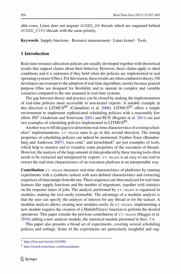
The steps for using rt-muse are illustrated in Fig. 1. The first step is the creationof a set-up file (in JSON format) that specifies the characteristics of the platform thatwe want to extract. The format of the configuration file is described in Sect. 5.
To avoid the bias introduced by the measuring infrastructure, the target machinethat runs the experiments and the host machine collecting and analyzing the executiontraces are different.
Once the configuration file is completed, the invocation of a script file at the hostmachine takes care of:
– Copying the configuration file to the target machine;– starting the experiments at the target machine.While the experiment is in progress,the target machine sends timestamps (via UDP datagrams) to the host machine thatcollects them;
– as soon as the experiment terminates, the target machine informs the host machine,which analyzes the data collected in accordance to the measurements requestedby the user.
During run-time, the timestamping infrastructure records the instant ti, j when thej-th execution of the job body belonging to the thread τi starts and the processingunit index πi, j . To record these timestamps, as well as to monitor other kernel events(thread migrations, scheduler invocation, etc.), we use trace-cmd,3 the user-space
3 http://lwn.net/Articles/410200/.
123
860 Real-Time Syst (2017) 53:857–885
Target machineHost machine
launchingthe script file
transferingthe configuration file
start ofthe experiment
experimentin progress
collectingtimestamps
analysisof data
end ofthe experiment
preparingthe configuration file
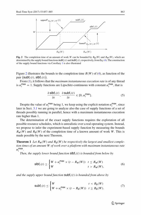
Fig. 1 Steps of rt-muse measurement procedure
front end for Ftrace.4 Ftrace is a lightweight tracer of kernel events developed bySteven Rostedt, one of the Linux kernel developers. Together with kernel events, suchas thread migrations or context switches, it can monitor user-defined events. On x86machines, Ftrace has nanoseconds precision.
Events can be collected by Ftrace in two ways: (1) stored in a buffer, which isthen flushed to disk when full, or (2) sent via User Datagram Protocol (UDP) to alistener instance of Ftrace running on a remote machine. Due to disk writing, if thecollector is executed on the same machine, there is a risk of service outage. This isespecially true if a large number of events is generated. To avoid this problem andto minimize the impact of the tool itself on the monitored experiment, we used theremote monitoring via UDP. The drawback of using UDP is the possibility of losingsome events. Although this never happened in the experiments reported in the paper,rt-muse is capable to reconstruct any missing event, by linearly interpolating thetwo neighboring ones.
rt-muse is invoked on a host machine and performs the following steps:
1. It sends the experiment description, formatted as described in Sect. 4, to the targetmachine, which is the one actually running the experiment;
2. It starts listening events sent by the target machine;
4 http://elinux.org/Ftrace.
123
Real-Time Syst (2017) 53:857–885 861
3. It communicates to the target machine to start the experiment run;4. It collects all received events until the target communicates the completion of the
experiment;5. It performs all the analysis modules requested by the user.
After the script file on the host machine has terminated, the user can read the outputof the experiment in a human readable form.
Finally, rt-muse is freely available on-line.5
Organization of the paper In the following, Sect. 3 describes the analysis modulesavailable. We start with the analysis to highlight what are the benefits of analyzing ataskset execution tracewithrt-muse. The paper then describes the applicationmodeland how it is possible to construct a synthetic taskset that models the real applicationin Sect. 4. rt-muse focuses on one specific type of applications (applications thatrepeats the same job continuously, like multimedia applications, streaming services,image analysis software and many others). Sections 5 and 6 then describe how the toolcan be used, and the results of the experiments that we have conductedwith rt-muse.Finally, Sect. 7 discusses related research efforts and Sect. 8 concludes the paper.
3 The analysis capabilities of rt-muse
This section describes the analysis modules offered by rt-muse. Each of the follow-ing subsections focuses on one of specific module currently implemented. rt-museis engineered to make it simple to add a new analysis module and to use the dataproduced by other modules for further investigations.
First, Sect. 3.1 describes the supply analysis module and the additional backgroundand definitions necessary to understand the analysis method. The supply modulecomputes an experiment-based approximation of the lower and upper supply boundfunctions of the computing resource allocated to a single thread as well as the boundsto the overall resource allocated to a set of threads. The section also lists several prop-erties, which are exploited for computing bounds to the supply functions. Second, inSect. 3.2 we describe the runmap module, which computes a map with informationabout where threads are executed. Third, in Sect. 3.3 we introduce the migration mod-ule, that computes the migrations experiences by each thread. Finally, in Sect. 3.4 weintroduce the statistical module that computes statistics about the average responsetime of jobs.
3.1 The supply analysis module
The supply analysis module aims at extracting an experiment-based supply functionfrom the trace of execution of the threads in the taskset. For each of the threadswe want to approximate the computational capacity offered by the platform with apowerful analysis tool. Supply functions have been used, possibly under differentnames in different contexts [e.g. service curves in network/real-time calculus (Cruz
5 https://github.com/martinamaggio/rt-muse.
123

862 Real-Time Syst (2017) 53:857–885
1991; Baccelli et al. 1992; Thiele et al. 2000)], to model the availability of differenttypes of resource: processing time of a single (Mok et al. 2001; Lipari and Bini 2003;Shin and Lee 2003) or multi-core (Bini 2009; Xu et al. 2015) platform, network (Cruz1991; Almeida et al. 2002), memory (Yun et al. 2016; Åkesson and Goossens 2011),and I/O (Pellizzoni et al. 2008). However, this is the first instance in which a supplyfunction is constructed based on the experimental execution trace.
To understand how supply functions are extracted from the application execution,let us first define an execution platform P as any mechanism that provides computingcapacity [such as a virtual machine, a priority level of a scheduler, or a periodicresource (Lipari and Bini 2003; Shin and Lee 2003)]. The supply analysis modulecomputes the experiment-based supply lower (respectively upper) bound functions˜slbf(t) (resp. ˜subf(t)) of the platform P , based on actual measurements.
The instrument of the supply module to measure the supply functions of a platformP , is a set T = {τ1, . . . , τn} of n threads which are going to be executed over theplatform itself. Each of the n threads τi ∈ T executes forever the same job in loop,with nominal duration ei . The job body can be configured by the user, as described inSect. 4, to test the response of the platform to different types of loads. For the durationof the experiment, the start time ti, j of the j-th job of the i-th thread is recordedby the monitoring infrastructure. The supply module extracts the supply lower andupper bounds by comparing the length of sequences of jobs with their nominal value.Intuitively, the longer the jobs take, the smaller is the amount of computing capacitydelivered by the platform P .
In the following we present our implementation choices for the supply module.Before, we recall some background on supply functions. The resource allocation oper-ated by the scheduler to thread τi is modeled by means of a scheduling function ξi (t)with the standard interpretation
ξi (t) ={1 τi runs at t0 otherwise.
(1)
The supply lower bound function slbfi (t) and the supply upper bound functionsubfi (t) of thread τi are functions such that (Mok et al. 2001; Lipari and Bini 2003;Shin and Lee 2003)
slbfi (b − a) ≤∫ b
aξi (t) dt ≤ subfi (b − a), (2)
meaning that slbfi (t) and subfi (t) are lower and upper bounds to the amount ofresource allocated to the thread τi in any interval of length t .
Supply functions also determine bounds to the completion time R(W ) of anyamount of work W to be made by the thread τi . In fact
Rb(W ) ≤ R(W ) ≤ Rw(W ), (3)
with Rb(W ) and Rw(W ) defined as
{Rw(W ) = sup{t : slbfi (t) < W }Rb(W ) = inf{t : subfi (t) ≥ W }. (4)
123
Real-Time Syst (2017) 53:857–885 863
W
Rb(W ) Rw(W )
subfi(t)
slbfi(t)
upperFRb(W ),W (t)
lowerFRw(W ),W (t)
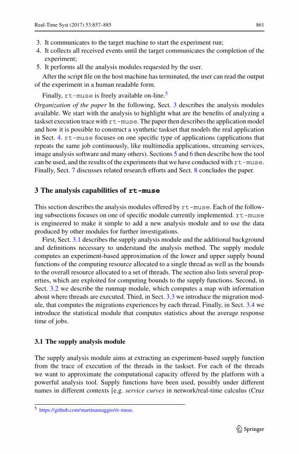
Fig. 2 The completion time of an amount of work W can be bounded by Rb(W ) and Rw(W ), which aredeterminedby the supply bound functionssubfi (t) andsubfi (t), respectively, fromEq. (4). The constructionof the supply bound functions via Corollary 1 is also illustrated
Figure 2 illustrates the bounds to the completion time R(W ) of (4), as function of thepair
(subfi (t), slbfi (t)
).
From (1), it follows that the maximum instantaneous execution rate is of any threadis αmax
i = 1. Supply functions are Lipschitz-continuous with constant αmaxi , that is
∂ slbfi (t)∂t
,∂ subfi (t)
∂t∈ [0, αmax
i ]. (5)
Despite the value of αmaxi being 1, we keep using the explicit notation αmax
i , sincelater in Sect. 3.1 we are going to analyze also the case of supply functions of a set ofthreads possibly running in parallel, hence with a maximum instantaneous executionrate higher than 1.
The determination of the exact supply functions requires the exploration of allpossible resource schedules, which is unrealistic over a real operating system. Instead,we propose to infer the experiment-based supply function by measuring the boundsRw(W ) and Rb(W ) of the completion time of a known amount of work W . This ismade possible by the next Theorem.
Theorem 1 Let Rw(W ) and Rb(W ) be respectively the largest and smallest comple-tion times of an amount W of work over a platform with maximum instantaneous rateαmax
i .Then, the supply lower bound function slbfi (t) is bounded from below by
slbfi (t) ≥{
W + αmaxi × (t − Rw(W )) t ≤ Rw(W )
W t > Rw(W ),(6)
and the supply upper bound function subfi (t) is bounded from above by
subfi (t) ≤{
W t < Rb(W )
W + αmaxi × (t − Rb(W )) t ≥ Rb(W ).
(7)
123

864 Real-Time Syst (2017) 53:857–885
Proof First, we prove the Theorem for the slbfi (t). By the definition of Rw(W ) in (4),it follows that
t > Rw(W ) ⇒ slbfi (t) ≥ W. (8)
In fact, if there is any t∗ > Rw(W )with slbfi (t∗) ≥ W , then Rw(W )would be at leastas big as t∗, which is a contradiction.
For any t ≤ Rw(W ) we invoke the Lipschitz-continuity of slbfi (t) with constantαmax
i , that is
slbfi (Rw(W )) − slbfi (t) ≤ αmaxi (Rw(W ) − t)
slbfi (t) ≥ slbfi (Rw(W )) + αmaxi (t − Rw(W )).
From (4), since Rw(W ) is the supremum of a set, then there is a sequence {tk}k∈Nwithin {t : slbfi (t) < W } such that limk tk = Rw(W ) and limk slbfi (tk) = W .From the continuity of slbfi (t), it follows that slbfi (Rw(W )) = W and then from theLipschitz-continuity
t ≤ Rw(W ) ⇒ slbfi (t) ≥ W + αmaxi (t − Rw(W )), (9)
which proves, together with (8), the lower bound on slbfi (t) of (6). The proof of (7)is analogous and it omitted for brevity. ��
The inequalities (6) and (7), can be written more compactly as
∀t, slbf(t) ≥ lowerFRw(W ),W (t)
∀t, slbf(t) ≤ upperFRb(W ),W (t)
respectively, with the auxiliary functions lowerFx,y(t) and upperFx,y(t) illustratedin 2, and defined as
lowerFx,y(t) ={
y + αmax × (t − x) t ≤ x
y t > x,(10)
upperFx,y(t) ={
y t < x
y + αmax × (t − x) t ≥ x .(11)
Since the bounds of (6) and (7) hold for any amount of work W , the next corollaryfollows.
Corollary 1 Let
– lowerFx,y(t) and upperFx,y(t) be defined as in (10) and (11), respectively, and– Rw(W ) and Rb(W ) be longest and shortest completion time of an amount of work
W over a platform with maximum instantaneous execution rate αmaxi .
123
Real-Time Syst (2017) 53:857–885 865
Then the following bounds on the slbfi (t) and subfi (t) hold
slbfi (t) ≥ supW≥0
{lowerFRw(W ),W (t)
}(12)
subfi (t) ≤ infW≥0
{upperFRb(W ),W (t)
}. (13)
Equations (12), (13) provide an alternate definition of the bounds to supply func-tions. The advantage of (12), (13) over the standard definitions of supply functions isthat they depend on the bounds Rw(W ) and Rb(W ) of the completion time of the workW made by thread τi . These values, in fact, can be measured by targeted experimentsand used, through (12) and (13), to compute the experiment-based supply functions.More precisely, the steps made by rt-muse to measure the supply functions of aplatform are
1. the set of threads {τ1, . . . , τn}, each one with nominal duration ei , are created bythe user (Sect. 4 describes how);
2. from the execution traces, the sequence of timestamps ti, j of the start time of thej-th job of τi is extracted ( j from 0 to the index maxJi of the latest timestamp);
3. from the sequence of timestamps {ti, j }maxJij=0 , following sequences
∀k = 0, . . . ,maxJi si,k = maxj=0,...,maxJi −k
{ti, j+k − ti, j }∀k = 0, . . . ,maxJi si,k = min
j=0,...,maxJi −k{ti, j+k − ti, j },
are computed (notice, it is always si,0 = si,0 = 0);4. since each τi is structured as forever loop,we approximated the longest and shortest
time to complete an amount of work equal to k × ei as follows
Rw(k × ei ) ≈ si,k Rb(k × ei ) ≈ si,k . (14)
5. finally, in accordance to the bounds of (12) and (13), we define the experiment-based supply upper/lower bound functions as
˜slbfi (t) = maxk=0...,maxJi
{lowerFsi,k ,kei (t)
}(15)
˜subfi (t) = mink=0...,maxJi
{upperFsi,k ,kei
(t)}. (16)
For thread τi , the job nominal length ei represents the duration of the job bodyin ideal conditions (with no interference by the execution of other threads). In ourexperiment-based computation, this value is set to
ei = si,1, (17)
that is the shortest duration among all job of τi in the experiment. The user can alsospecify any other value. Since the job lengths extracted from the timestamps sequence
123

866 Real-Time Syst (2017) 53:857–885
have to be compared against the nominal length ei , setting ei to a bigger value maylead to too optimistic conclusions about the computing capacity of the platform, whilesetting ei smaller than si,1 may be too conservative.
To summarize the content of supply functions in amore compact andunderstandableform, they are often abstracted by the bandwidth and the delay. More precisely, with
a given˜slbfi (t), we say that the supply lower bound function has bandwidth αi anddelay �i if
∀t, ˜slbfi (t) ≥ αi (t − �i ). (18)
Among the many pairs (α,�) satisfying (18), we choose the one such that thecorresponding linear lower bound better approximate the exact supply lower boundfunction slbf(t). Such a pair corresponds to the solution of the followingmaximizationproblem
maximize∫ H
�
α(t − �)
such that slbf(t) ≥ α(t − �) ∀t
with H being a user-defined time-horizon of interest. In fact, the area below the linearlower bound over the interval of interest [0, H ] can be considered a measure of thetightness of the linear lower bound.
Analogously as in (18), we also define the bandwidth and delay of the supply upperbound function as any pair (αi ,�i ) such that:
∀t, ˜subfi (t) ≤ αi (t − �i ). (19)
Notice that from the property that ˜subfi (0) = 0, it follows that �i is always going tobe non-positive. Similarly to the lower bound case, to among all linear upper boundssatisfying (19), our tool computes explicitly the pair (αi ,�i ) among the feasible ones,such that the area below the linear upper boundover the interval [0, H ] isminimized.Toenable the computation of different linear upper/lower bounds, the tool also computesthe convex hull of both the lower and the upper bound functions.
The supplymodule also allows the characterization of the overall computing capac-ity delivered by the platform P to the entire set of n threads T . These measures aredenoted by the subscript “∗” rather than “i” of the per-thread analysis. The steps areexactly the same as for the per-thread analysis, with the following adaptation
1. the overall schedule is defined by
ξ∗(t) =∑τi ∈T
ξi (t),
2. the maximum instantaneous execution rate is set to αmax∗ = min(n, m), with mbeing the number of processors of the platform, and
123

Real-Time Syst (2017) 53:857–885 867
3. the timestamps are
{t∗,k} =n⋃
i=1
{ti,k},
since, in this case, we aim at measuring the amount of computation delivered bythe platform to any thread.
After the analysis of the overall platform P is completed, the results are the supply
function bounds˜slbf∗(t),˜subf∗(t), the bandwidth/delay pair of the linear lower bound(α∗,�∗), and the pair of the linear upper bound (α∗,�∗).
3.2 The runmap analysis module
At the begin of all jobs, Ftrace collects both the timestamp ti, j as well as the index ofthe CPU on which the j-th job by the i-th thread started on, denoted with πi, j . Thisinformation is used by the runmap analysis module, together with the total number ofjobs terminated by each thread, to compute the runmap. For each CPU included in theaffinity mask of the thread, the tool reports the percentage of jobs that started on thatCPU. This analysis can only be performed per thread.
3.3 The migration analysis module
For each thread, we compute the number of migrations experienced by the threadduring its execution. This analysis can only be performed per thread. The migrationmodule analyzes migrations data and allows one to compute the frequency of migra-tion over time. This will make the information about conditions in which thread areconstantly migrated more accessible to the user, who can then understand when thelimits of the platform have been reached.
3.4 The statistical analysis module
If we define the random variable si,k as the time it takes to execute k consecutive jobsof the thread τi (i.e., the time elapsing between the start times of k + 1 consecutivejobs), we can say that the supply analysis module provides information about the tworandom variables min{si,k} and max{si,k}. The statistical analysis module, instead,investigates the mean and the variance of the random variable si,k . If we assume thatthe timestamps of the start times of τi ’s jobs are indexed from 0 to maxJi , then thestatistical analysis module computes, for all k = 1, . . . ,maxJi , the average μi,k andthe variance σ 2
i,k , as described below
μi,k =∑maxJi −k
j=0 (ti, j+k − ti, j )
maxJi − k + 1(20)
123

868 Real-Time Syst (2017) 53:857–885
σ 2i,k =
∑maxJi −kj=0 (μi,k − (ti, j+k − ti, j ))
2
maxJi − k + 1(21)
therefore avoiding the last k−1 jobs, thatwould not contribute to ameaningful estimateof the time it takes to execute k jobs.
4 Modeling a taskset with rt-muse
The goal of rt-muse is to measure the computing capacity delivered by theexecution platform to different types of workloads. Such a feature is realized byallowing the testing threads T to be configured by the user. For this purpose, thejob body of each thread τi is composed by the sequential concatenation of pi
job phases denoted by φi,1, φi,2, . . . , φi,pi . Each phase φi,k belongs to a set
of available phases. Currently, the tool offers the following set of phases ={φcompute, φlock, φmemory, φshared, φuser}. Each phase may be configured throughsome input parameters, as described below.
The phase φcompute(�), called compute phase, is configured with a positive integer�. The execution of the phase φcompute(�) keeps the CPU busy for a time proportionalto �. In our current implementation, this phase executes � floating point operations.This can be used to simulate any computational intensive work such as the run of acontrol algorithm, the aggregation of data from different sensors or else.
The phase φlock(�, r), called lock phase, is configured with a positive integer �
and an index r of a shared resource. The body of the phase is exactly the same as thecompute phase.However, before starting the execution of themathematical operations,the thread locks the shared resource r . The lock is released at the end of the execution.Resource identifiers are numbered from 0 to R − 1, where R is the total numberof available resources, as specified in the test configuration file. We use the defaultpthread_mutex_lock function offered by glibc version 2.19. This phase can,therefore, be used to evaluate the impact of shared resources on the overall computingcapacity and to test different locking protocols.
The phase φmemory(�, m), called memory phase, is configured with a positive inte-ger � and a size m of memory to be used. The body of the phase is exactly the same asthe compute phase. However, before entering the computation part, the phase dynam-ically allocates an amount of memory corresponding to m double values on the heapand saves the results of the mathematical computation in the allocated vector. When-ever the result storage reaches the end of the vector, it restarts from the beginning. Thisphase can be used to test the platform in presence of memory writing and to evaluatethe impact of cache sizes on the performance delivered to the running applications.
The phase φshared(�), called shared phase, is configured with a positive integer �.The phase behaves similarly to the memory phase, but it writes the data to a memorybuffer shared among all the threads (rather than in a private buffer as in φmemory). Theshared memory is locked before usage and the lock is released when the � operationsare completed. The size of the shared memory buffer is specified as a configurationparameter for the entire application and thememory is allocated on the heap at start-up.
123
Real-Time Syst (2017) 53:857–885 869
This phase can be used to evaluate the performance degradation in presence of sharedmemory.
Finally, the phase φuser offers the user the possibility to define any user-specificphase. During this phase, the user function is invoked. The code of this phase can bemodified by the user to analyze the computing capacity delivered by the platform toany type of application, which cannot be precisely described by any sequence of thepredefined phases.
5 Specification of experiments
As anticipated in Sect. 2, an experiment is defined by a configuration file that specifiesthe taskset characteristics and the execution platform characteristics. This file is for-matted using the JavaScript Object Notation (JSON6). As illustrated in the exampleof Listing 1, and has four main sections (“objects” in the JSON terminology):
1. global, specifying the global settings,2. resources, specifying the available resources,3. shared, denoting the shared memory size, and4. threads, describing the threads in T to be executed.
Theglobal configuration section (lines 1–4 in the example of Listing 1) allows theuser to specify the default scheduling policy to be used.Currently, onlyLinuxmachinesare allowed, and the scheduling classes can be chosen among SCHED_OTHER,SCHED_RR, SCHED_FIFO and SCHED_DEADLINE, which are implemented in thelatest kernel (at line 2, SCHED_RR is specified as default). Also, the duration of theexperiment in seconds is specified in the global section (10 seconds in the example,at line 3). The resources section (line 6 in the example) reports the number R oftotal different shared resources to be used by any φlock phase. In the lock phase, onecan specify that the thread locks the resource r = 0, . . . , R − 1. The section shared(line 7 in the example) specifies the size in bytes of the shared memory buffer to beshared by the φshared thread phases. Such a buffer is protected with an additional lock(not belonging to the R mutexes specified in the resources section).
1 { "global" : {2 "default_policy" : "SCHED_RR",3 "duration" : 10,4 "analysis": { "supply": true }5 },6 "resources": 2,7 "shared": 50,8 "threads": {9 "thread1": {
10 "priority": 10,11 "cpus": [0,1,2],12 "phases": {13 "c0": { "loops": 1000 },14 "l0": { "loops": 2000, "res": 0 },15 "s0": { "loops": 1000 },
6 http://www.json.org.
123

870 Real-Time Syst (2017) 53:857–885
16 "l1": { "loops": 3000, "res": 1 },17 "m0": { "loops": 1000, "memory": 10 },18 "c1": { "loops": 5000 }19 },20 "analysis": { "supply": true,21 "runmap": true,22 "migrations": true,23 "statistical": true }24 },25 "thread2": {26 "cpus": [0,1],27 "policy": "SCHED_DEADLINE",28 "budget": 1000,29 "period": 2000,30 "phases": {31 "c0": { "loops": 5000 },32 "m0": { "loops": 1000, "memory": 100 },33 "l0": { "loops": 10000, "res": 1 }34 } } } }
Listing 1 Example of JSON test configuration file.
The threads τ ∈ T are described in thethread section (lines 8–34 in the example).For each thread τi the scheduling parameters are specified. These parameters are usedby the scheduler to select the threads to be executed over the execution platform P (inthe example, τ1 is scheduled by the default scheduling policySCHED_RRwith priority10 set at line 10, while at lines 27–29 τ2 is set to be scheduled by SCHED_DEADLINEwith budget 1000 and period 2000 nanoseconds). Also, for each thread it is possibleto specify its affinity, that is the subset of the available CPUs on which the thread isallowed to execute (in the example, τ1 can execute only on CPUs 0, 1, and 2, while τ2can execute only on CPUs 0 and 1). If left unspecified, the thread can migrate over allthe available CPUs.
Finally, for each thread τi the phases section contains the list of the pi phases tobe executed in sequence. Each phase has a name and the corresponding parameters.The name of the phase identifies its type. A phase name that starts with the letter c is aφcompute(�) phase and expects to receive the parameter �. A phase name starting withthe letter l indicates a lock phase φlock(�, r) and should receive two parameters, thenumber of iterations � and the resource r to be locked. A phase name starting with theletter m denotes a memory phase φmemory(�, m) and takes two parameters, the numberof iterations � and the amount of memory to be used m. Finally, a phase name startingwith the letter s identify a shared phase φshared(�) and receives one parameter, thenumber of iterations �. Phases of the same type may repeat within the thread body.In the example, τ1 has p1 = 5 phases described in lines 12–19. According to thespecification of Listing 1, the phases of τ1 are:
1. φ1,1 = φcompute(1000), that is a loop of 1000 mathematical operations,2. φ1,2 = φlock(2000, 0), that is a loop of 2000 mathematical operations while lock-
ing resource 0,3. φ1,3 = φshared(1000), that is it computes 1000 operations on the shared memory
buffer of size 50 (as specified at line 7),4. φ1,4 = φlock(1000, 1), that is τ1 uses resource 1, and then does 1000 iterations,
123
Real-Time Syst (2017) 53:857–885 871
5. φ1,5 = φmemory(1000, 10), that is τ1 does 1000 iterations writing circularly in amemory area of 10 elements, and finally
6. φ1,6 = φcompute(5000), that is a loop of 5000 mathematical operations.
Thread τ2 of the example, instead, has the following phases: φ2,1 = φcompute(5000),φ2,2 = φmemory(1000, 100), and φ2,3 = φlock(10000, 1).
The analysis section can be specified within each thread specification as well aswithin the global section. In both cases, it lists the name of the analysis modules tobe executed. In case the analysis element is missing (such as for τ2 in the example),then the corresponding thread data is not analyzed, although executed. This feature canbe used to create someworkload interferingwith the threads to bemonitored.When theanalysis section is present in theglobal section, the corresponding analysismod-ules are performedover thedata aggregated fromall threads that contain ananalysissection. Such a type of aggregated analysis can be used to determine the overall char-acteristics of the platform (such as the overall delivered computing capacity).
5.1 Example of results
To better illustrate the output of rt-muse, we present an example with 6 threadsall equal to each other. We assigned them the SCHED_OTHER scheduling class andset an affinity mask that contains CPUs [1, 2, 3], meaning that all the 6 threads wereconfined to run over 3 among the 4 CPUs available on our platform. All thread bodieswere composed by the only one phase φi,1 = φcompute(100000), for all i = 1, . . . , 6.The experiment lasted 100 seconds.
The actual duration of the monitored window was 99.0567 s. Compared to theduration of the experiment (set to 100 s), it means that it took about one second to startup the tool, create the threads, take first scheduling decisions, etc. before the first jobof all 6 threads was activated.
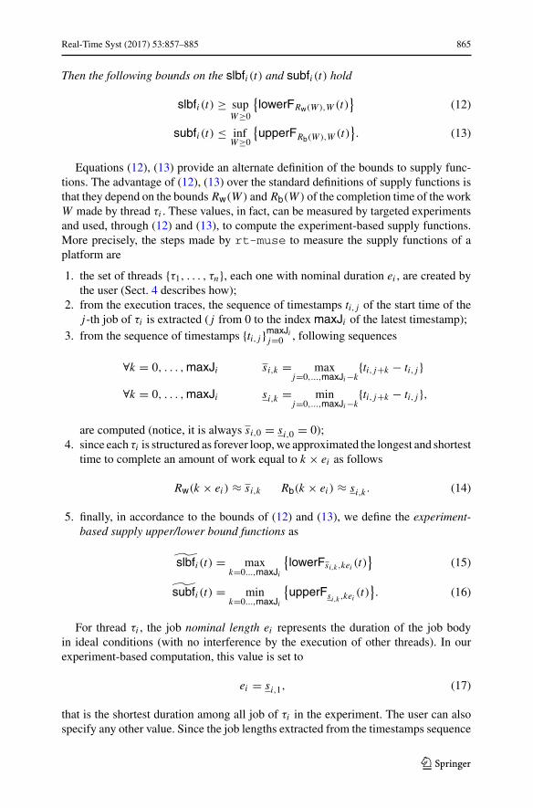
Let us illustrate the results of the analysis of thread τ3 (anyother selectionwould givesimilar data, as all threads are the same). Thread τ3 released 35838 (denoted bymaxJ3in Sect. 3.1) jobs in the analysis window. The number of job migrations measured bythe migrations module is 220. Thread τ3 did run over the 3 CPUs according tothe shares [0.009, 0.440, 0.551]. The experiment-based supply lower/upper bounds˜slbf3(t) and ˜subf3(t) are plotted in Fig. 3. Notice that, to illustrate the informationover different timescales, the lower-left corner of the top figure is properly magnifiedbelow. Lower and upper linear bounds, with parameters (α3,�3) and (α3,�3), arealso drawn in dashed lines. Finally, we observe that any valid linear bound, other thanthe ones explicitly computed by our method, can be determined by evaluating only
the points over the convex hull of˜slbf3(t) (or ˜subf3(t)) provided with the results. Thevertices of the supply function along the convex hull are also drawn in the figure.
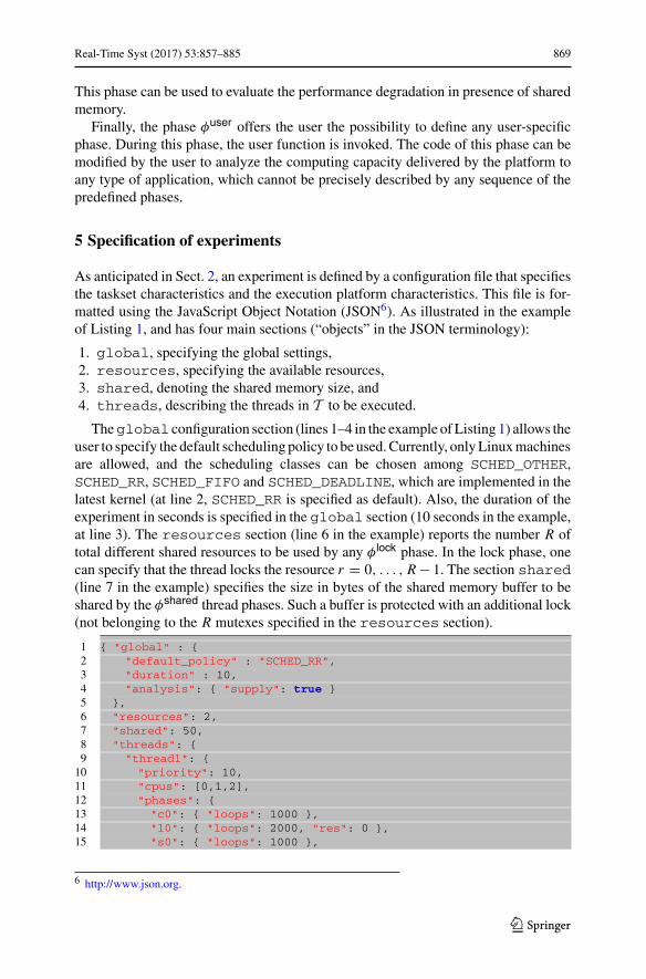
For the same thread τ3, Fig. 4 illustrates the standard deviation σ3,k , that is thesquare root of the expression of (21). As illustrated in the figure, σ3,k grows up to amaximum and then decreases to 0 when k ← maxJ3. In fact, when k grows, thenthe sample space over which the variance is computed shrinks. Unless the schedulingalgorithm of the platform P can provide some level of determinism in the resource
123

872 Real-Time Syst (2017) 53:857–885
125
100
75
50
25
00 25 50 75 100 125 150 175 200 225 250
0 0.5 1 1.5 2 2.5 3 3.5 4 4.5 5
2.5
2
1.5
1
0.5
0
[msec]
[msec]
[sec]
[sec]
slbf(t)
subf(t)
max{0, α(t − Δ)}min{αmaxt, α(t − Δ)}convex hull of slbf(t)
convex hull of subf(t)
Fig. 3 Illustration of the results of the supply analysis module
0 5 10 15 20 25 30 35 40
0.6
0.4
0.2
0.8
0
σ3,k
k × 103
Fig. 4 Standard deviation σ3,k over k, as computed by the statistical analysis module
allocation to k consecutive jobs for some k, a decrease of σi,k should be interpreted asan indication of a short experiment duration.
123
Real-Time Syst (2017) 53:857–885 873
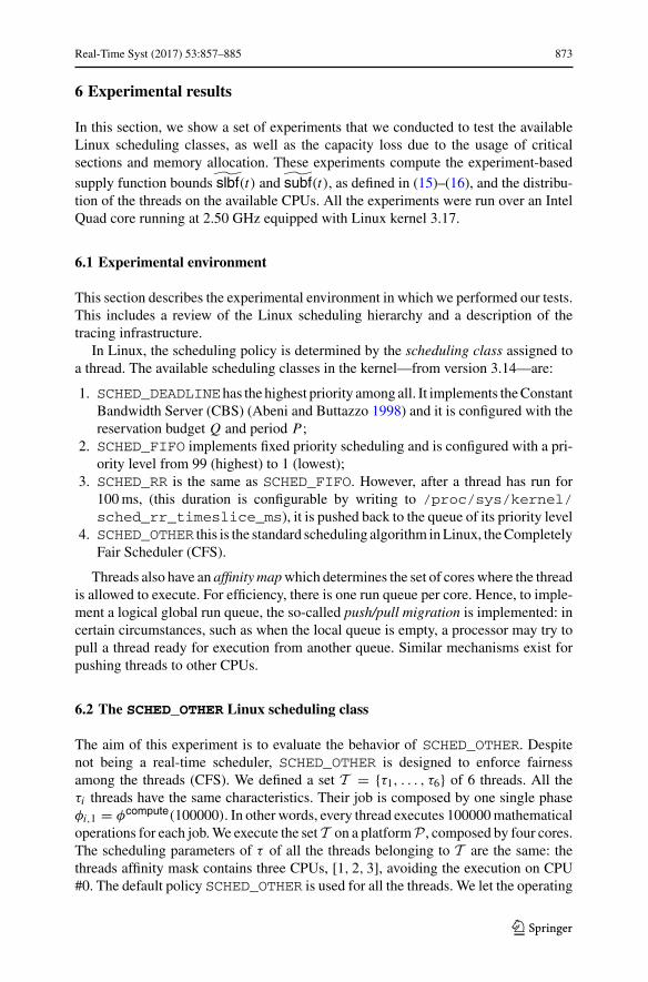
6 Experimental results
In this section, we show a set of experiments that we conducted to test the availableLinux scheduling classes, as well as the capacity loss due to the usage of criticalsections and memory allocation. These experiments compute the experiment-based
supply function bounds˜slbf(t) and ˜subf(t), as defined in (15)–(16), and the distribu-tion of the threads on the available CPUs. All the experiments were run over an IntelQuad core running at 2.50 GHz equipped with Linux kernel 3.17.
6.1 Experimental environment
This section describes the experimental environment in which we performed our tests.This includes a review of the Linux scheduling hierarchy and a description of thetracing infrastructure.
In Linux, the scheduling policy is determined by the scheduling class assigned toa thread. The available scheduling classes in the kernel—from version 3.14—are:
1. SCHED_DEADLINEhas the highest priority among all. It implements theConstantBandwidth Server (CBS) (Abeni and Buttazzo 1998) and it is configured with thereservation budget Q and period P;
2. SCHED_FIFO implements fixed priority scheduling and is configured with a pri-ority level from 99 (highest) to 1 (lowest);
3. SCHED_RR is the same as SCHED_FIFO. However, after a thread has run for100ms, (this duration is configurable by writing to /proc/sys/kernel/sched_rr_timeslice_ms), it is pushed back to the queue of its priority level
4. SCHED_OTHER this is the standard scheduling algorithm inLinux, theCompletelyFair Scheduler (CFS).
Threads also have an affinity mapwhich determines the set of coreswhere the threadis allowed to execute. For efficiency, there is one run queue per core. Hence, to imple-ment a logical global run queue, the so-called push/pull migration is implemented: incertain circumstances, such as when the local queue is empty, a processor may try topull a thread ready for execution from another queue. Similar mechanisms exist forpushing threads to other CPUs.
6.2 The SCHED_OTHER Linux scheduling class
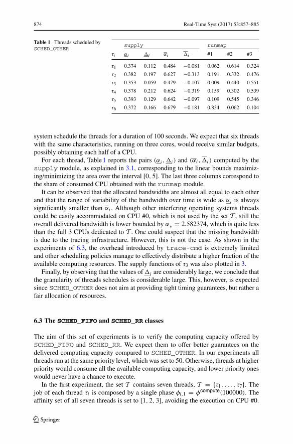
The aim of this experiment is to evaluate the behavior of SCHED_OTHER. Despitenot being a real-time scheduler, SCHED_OTHER is designed to enforce fairnessamong the threads (CFS). We defined a set T = {τ1, . . . , τ6} of 6 threads. All theτi threads have the same characteristics. Their job is composed by one single phaseφi,1 = φcompute(100000). In other words, every thread executes 100000mathematicaloperations for each job.We execute the set T on a platformP , composed by four cores.The scheduling parameters of τ of all the threads belonging to T are the same: thethreads affinity mask contains three CPUs, [1, 2, 3], avoiding the execution on CPU#0. The default policy SCHED_OTHER is used for all the threads. We let the operating
123
874 Real-Time Syst (2017) 53:857–885
Table 1 Threads scheduled bySCHED_OTHER
supply runmap
τi αi �i αi �i #1 #2 #3
τ1 0.374 0.112 0.484 −0.081 0.062 0.614 0.324
τ2 0.382 0.197 0.627 −0.313 0.191 0.332 0.476
τ3 0.353 0.059 0.479 −0.107 0.009 0.440 0.551
τ4 0.378 0.212 0.624 −0.319 0.159 0.302 0.539
τ5 0.393 0.129 0.642 −0.097 0.109 0.545 0.346
τ6 0.372 0.166 0.679 −0.181 0.834 0.062 0.104
system schedule the threads for a duration of 100 seconds. We expect that six threadswith the same characteristics, running on three cores, would receive similar budgets,possibly obtaining each half of a CPU.
For each thread, Table1 reports the pairs (αi ,�i ) and (αi ,�i ) computed by thesupply module, as explained in 3.1, corresponding to the linear bounds maximiz-ing/minimizing the area over the interval [0, 5]. The last three columns correspond tothe share of consumed CPU obtained with the runmap module.
It can be observed that the allocated bandwidths are almost all equal to each otherand that the range of variability of the bandwidth over time is wide as αi is alwayssignificantly smaller than αi . Although other interfering operating systems threadscould be easily accommodated on CPU #0, which is not used by the set T , still theoverall delivered bandwidth is lower bounded by α∗ = 2.582374, which is quite lessthan the full 3 CPUs dedicated to T . One could suspect that the missing bandwidthis due to the tracing infrastructure. However, this is not the case. As shown in theexperiments of 6.3, the overhead introduced by trace-cmd is extremely limitedand other scheduling policies manage to effectively distribute a higher fraction of theavailable computing resources. The supply functions of τ3 was also plotted in 3.
Finally, by observing that the values of �i are considerably large, we conclude thatthe granularity of threads schedules is considerable large. This, however, is expectedsince SCHED_OTHER does not aim at providing tight timing guarantees, but rather afair allocation of resources.
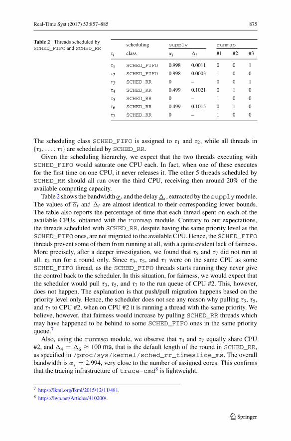
6.3 The SCHED_FIFO and SCHED_RR classes
The aim of this set of experiments is to verify the computing capacity offered bySCHED_FIFO and SCHED_RR. We expect them to offer better guarantees on thedelivered computing capacity compared to SCHED_OTHER. In our experiments allthreads run at the same priority level, which was set to 50. Otherwise, threads at higherpriority would consume all the available computing capacity, and lower priority oneswould never have a chance to execute.
In the first experiment, the set T contains seven threads, T = {τ1, . . . , τ7}. Thejob of each thread τi is composed by a single phase φi,1 = φcompute(100000). Theaffinity set of all seven threads is set to [1, 2, 3], avoiding the execution on CPU #0.
123
Real-Time Syst (2017) 53:857–885 875
Table 2 Threads scheduled bySCHED_FIFO and SCHED_RR
scheduling supply runmap
τi class αi �i #1 #2 #3
τ1 SCHED_FIFO 0.998 0.0011 0 0 1
τ2 SCHED_FIFO 0.998 0.0003 1 0 0
τ3 SCHED_RR 0 – 0 0 1
τ4 SCHED_RR 0.499 0.1021 0 1 0
τ5 SCHED_RR 0 – 1 0 0
τ6 SCHED_RR 0.499 0.1015 0 1 0
τ7 SCHED_RR 0 – 1 0 0
The scheduling class SCHED_FIFO is assigned to τ1 and τ2, while all threads in{τ3, . . . , τ7} are scheduled by SCHED_RR.
Given the scheduling hierarchy, we expect that the two threads executing withSCHED_FIFO would saturate one CPU each. In fact, when one of these executesfor the first time on one CPU, it never releases it. The other 5 threads scheduled bySCHED_RR should all run over the third CPU, receiving then around 20% of theavailable computing capacity.
Table2 shows the bandwidthαi and the delay�i , extracted by thesupplymodule.The values of αi and �i are almost identical to their corresponding lower bounds.The table also reports the percentage of time that each thread spent on each of theavailable CPUs, obtained with the runmap module. Contrary to our expectations,the threads scheduled with SCHED_RR, despite having the same priority level as theSCHED_FIFO ones, are not migrated to the available CPU. Hence, the SCHED_FIFOthreads prevent some of them from running at all, with a quite evident lack of fairness.More precisely, after a deeper investigation, we found that τ5 and τ7 did not run atall. τ3 run for a round only. Since τ3, τ5, and τ7 were on the same CPU as someSCHED_FIFO thread, as the SCHED_FIFO threads starts running they never givethe control back to the scheduler. In this situation, for fairness, we would expect thatthe scheduler would pull τ3, τ5, and τ7 to the run queue of CPU #2. This, however,does not happen. The explanation is that push/pull migration happens based on thepriority level only. Hence, the scheduler does not see any reason why pulling τ3, τ5,and τ7 to CPU #2, when on CPU #2 it is running a thread with the same priority. Webelieve, however, that fairness would increase by pulling SCHED_RR threads whichmay have happened to be behind to some SCHED_FIFO ones in the same priorityqueue.7
Also, using the runmap module, we observe that τ4 and τ7 equally share CPU#2, and �4 = �6 ≈ 100 ms, that is the default length of the round in SCHED_RR,as specified in /proc/sys/kernel/sched_rr_timeslice_ms. The overallbandwidth is α∗ = 2.994, very close to the number of assigned cores. This confirmsthat the tracing infrastructure of trace-cmd8 is lightweight.
7 https://lkml.org/lkml/2015/12/11/481.8 https://lwn.net/Articles/410200/.
123
876 Real-Time Syst (2017) 53:857–885
Table 3 Threads scheduled bySCHED_RR
supply runmap
τi αi �i �i #1 #2 #3
τ1 0.499088 0.103804 −0.101733 0 1 0
τ2 0.332735 0.201808 −0.202646 1 0 0
τ3 0.332756 0.202721 −0.202454 1 0 0
τ4 0.499114 0.102200 −0.197099 0 0 1
τ5 0.499065 0.104840 −0.101514 0 1 0
τ6 0.332763 0.202703 −0.202447 1 0 0
τ7 0.499093 0.197762 −0.102400 0 0 1
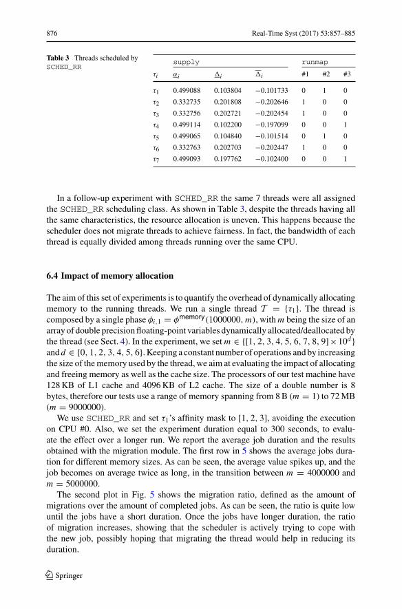
In a follow-up experiment with SCHED_RR the same 7 threads were all assignedthe SCHED_RR scheduling class. As shown in Table 3, despite the threads having allthe same characteristics, the resource allocation is uneven. This happens because thescheduler does not migrate threads to achieve fairness. In fact, the bandwidth of eachthread is equally divided among threads running over the same CPU.
6.4 Impact of memory allocation
The aim of this set of experiments is to quantify the overhead of dynamically allocatingmemory to the running threads. We run a single thread T = {τ1}. The thread iscomposed by a single phase φi,1 = φmemory(1000000, m), with m being the size of anarray of double precisionfloating-point variables dynamically allocated/deallocated bythe thread (see Sect. 4). In the experiment, we set m ∈ {[1, 2, 3, 4, 5, 6, 7, 8, 9]×10d }andd ∈ {0, 1, 2, 3, 4, 5, 6}.Keeping a constant number of operations andby increasingthe size of thememory used by the thread, we aim at evaluating the impact of allocatingand freeing memory as well as the cache size. The processors of our test machine have128KB of L1 cache and 4096KB of L2 cache. The size of a double number is 8bytes, therefore our tests use a range of memory spanning from 8B (m = 1) to 72MB(m = 9000000).
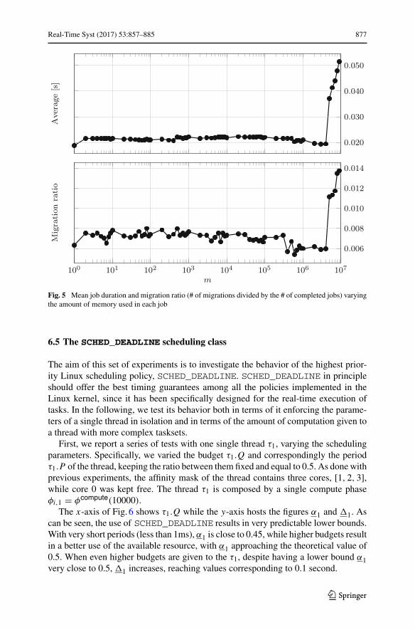
We use SCHED_RR and set τ1’s affinity mask to [1, 2, 3], avoiding the executionon CPU #0. Also, we set the experiment duration equal to 300 seconds, to evalu-ate the effect over a longer run. We report the average job duration and the resultsobtained with the migration module. The first row in 5 shows the average jobs dura-tion for different memory sizes. As can be seen, the average value spikes up, and thejob becomes on average twice as long, in the transition between m = 4000000 andm = 5000000.
The second plot in Fig. 5 shows the migration ratio, defined as the amount ofmigrations over the amount of completed jobs. As can be seen, the ratio is quite lowuntil the jobs have a short duration. Once the jobs have longer duration, the ratioof migration increases, showing that the scheduler is actively trying to cope withthe new job, possibly hoping that migrating the thread would help in reducing itsduration.
123
Real-Time Syst (2017) 53:857–885 877
0.020
0.030
0.040
0.050Average
[s]
100 101 102 103 104 105 106 107
0.006
0.008
0.010
0.012
0.014
m
Migration
ratio
Fig. 5 Mean job duration and migration ratio (# of migrations divided by the # of completed jobs) varyingthe amount of memory used in each job
6.5 The SCHED_DEADLINE scheduling class
The aim of this set of experiments is to investigate the behavior of the highest prior-ity Linux scheduling policy, SCHED_DEADLINE. SCHED_DEADLINE in principleshould offer the best timing guarantees among all the policies implemented in theLinux kernel, since it has been specifically designed for the real-time execution oftasks. In the following, we test its behavior both in terms of it enforcing the parame-ters of a single thread in isolation and in terms of the amount of computation given toa thread with more complex tasksets.
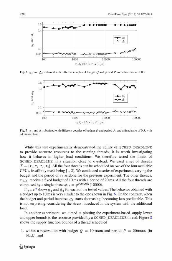
First, we report a series of tests with one single thread τ1, varying the schedulingparameters. Specifically, we varied the budget τ1.Q and correspondingly the periodτ1.P of the thread, keeping the ratio between them fixed and equal to 0.5. As done withprevious experiments, the affinity mask of the thread contains three cores, [1, 2, 3],while core 0 was kept free. The thread τ1 is composed by a single compute phaseφi,1 = φcompute(10000).
The x-axis of Fig. 6 shows τ1.Q while the y-axis hosts the figures α1 and �1. Ascan be seen, the use of SCHED_DEADLINE results in very predictable lower bounds.With very short periods (less than 1ms), α1 is close to 0.45, while higher budgets resultin a better use of the available resource, with α1 approaching the theoretical value of0.5. When even higher budgets are given to the τ1, despite having a lower bound α1very close to 0.5, �1 increases, reaching values corresponding to 0.1 second.
123
878 Real-Time Syst (2017) 53:857–885
100 1000 10000 100000
0.01
0.1
0.4
0.5
τ1.Q (0.5 × τ1.P ) [μs]
α1an
dΔ
1
α1Δ1
Fig. 6 α1 and �1 obtained with different couples of budget Q and period P and a fixed ratio of 0.5
100 1000 10000 100000
0.01
0.1
0.4
0.5
τ1.Q (0.5 × τ1.P ) [μs]
α1an
dΔ
1
α1Δ1
Fig. 7 α1 and �1 obtained with different couples of budget Q and period P , and a fixed ratio of 0.5, withadditional load
While this test experimentally demonstrated the ability of SCHED_DEADLINEto provide accurate resources to the running threads, it is worth investigatinghow it behaves in higher load conditions. We therefore tested the limits ofSCHED_DEADLINE in a situation close to overload. We used a set of threadsT = {τ1, τ2, τ3, τ4}. All the four threads can be scheduled on two of the four availableCPUs, its affinity mask being [1, 2]. We conducted a series of experiment, varying thebudget and the period of τ1 as done for the previous experiment. The other threads,τ{2..4} receive a fixed budget of 10ms with a period of 20ms. All the four threads arecomposed by a single phase φi,∗ = φcompute(10000).
Figure7 shows α1 and�1 for each of the tested values. The behavior obtained witha budget up to 10 ms is very similar to the one shown in Fig. 6. On the contrary, whenthe budget and period increase, α1 starts decreasing, becoming less predictable. Thisis not surprising, considering the stress introduced in the system with the additionalload.
In another experiment, we aimed at plotting the experiment-based supply lowerand upper bounds to the resource provided by a SCHED_DEADLINE thread. Figure 8shows the supply function bounds of a thread scheduled
1. within a reservation with budget Q = 10msec and period P = 20msec (inblack), and
123

Real-Time Syst (2017) 53:857–885 879
100
80
60
40
20
00 20 40 60 80 100 120 140 160 180 200
0 0.2 0.4 0.6 0.8 1 1.2 1.4 1.6 1.8 2
1
0.8
0.6
0.4
0.2
0
[msec]
[msec]
[sec]
[sec]
slbf(t), subf(t), Q = 10msec, P = 20msec
linear bounds, Q = 10msec, P = 20msec
slbf(t), subf(t), Q = 50msec, P = 100msec
linear bounds, Q = 50msec, P = 100msec
Fig. 8 Supply functions of a SCHED_DEADLINE thread
2. within a reservation with budget Q = 50msec and period P = 100msec (ingray).
Also, the linear bounds are drawn by dashed lines. In addition to the analized thread,7 more threads create load to the 4 CPUs, such that the total load by the 8 threads tothe 4 CPUs is about 3.5.
In the case of period P = 20msec, the lower bound to the bandwidth is α1 =0.495127, very close to the theoretical value of 0.5. Similarly, in the case of periodP = 100msec, the lower bound to the bandwidth is α1 = 0.495218.
6.6 Decrease of capacity with shared resources
The aim of this set of experiments is to investigate the variation in the total offeredcomputing capacity α∗ due to critical sections. To do so, we define a set of nthreads T = {τ1, . . . , τn} with n belonging to the set {3, 5, 10}. All jobs of allthreads are composed by two different phases: φi,1 = φlock(x × 10000, 0) and
123
880 Real-Time Syst (2017) 53:857–885
3
2.5
2
1.5
1
0.50 10 20 30 40 50 60 70 80 90 1005 15 25 35 45 55 65 75 85 95
[lock %]
α∗
n = 3
n = 5
n = 10
Fig. 9 Total computing capacity α∗ as the size of critical section varies
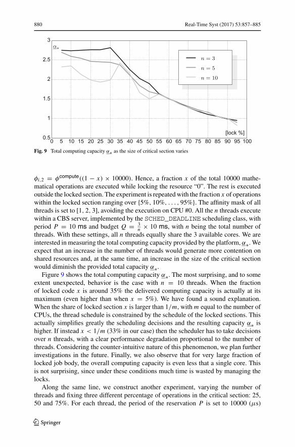
φi,2 = φcompute((1 − x) × 10000). Hence, a fraction x of the total 10000 mathe-matical operations are executed while locking the resource “0”. The rest is executedoutside the locked section. The experiment is repeatedwith the fraction x of operationswithin the locked section ranging over {5%, 10%, . . . , 95%}. The affinity mask of allthreads is set to [1, 2, 3], avoiding the execution on CPU #0. All the n threads executewithin a CBS server, implemented by the SCHED_DEADLINE scheduling class, withperiod P = 10 ms and budget Q = 3
n × 10 ms, with n being the total number ofthreads. With these settings, all n threads equally share the 3 available cores. We areinterested in measuring the total computing capacity provided by the platform, α∗. Weexpect that an increase in the number of threads would generate more contention onshared resources and, at the same time, an increase in the size of the critical sectionwould diminish the provided total capacity α∗.
Figure 9 shows the total computing capacity α∗. The most surprising, and to someextent unexpected, behavior is the case with n = 10 threads. When the fractionof locked code x is around 35% the delivered computing capacity is actually at itsmaximum (even higher than when x = 5%). We have found a sound explanation.When the share of locked section x is larger than 1/m, with m equal to the number ofCPUs, the thread schedule is constrained by the schedule of the locked sections. Thisactually simplifies greatly the scheduling decisions and the resulting capacity α∗ ishigher. If instead x < 1/m (33% in our case) then the scheduler has to take decisionsover n threads, with a clear performance degradation proportional to the number ofthreads. Considering the counter-intuitive nature of this phenomenon, we plan furtherinvestigations in the future. Finally, we also observe that for very large fraction oflocked job body, the overall computing capacity is even less that a single core. Thisis not surprising, since under these conditions much time is wasted by managing thelocks.
Along the same line, we construct another experiment, varying the number ofthreads and fixing three different percentage of operations in the critical section: 25,50 and 75%. For each thread, the period of the reservation P is set to 10000 (μs)
123
Real-Time Syst (2017) 53:857–885 881
0 20 40 60 80 100
0.5
1
1.5
2
2.5
Number of threads
α∗
α∗25% α∗50% α∗75%
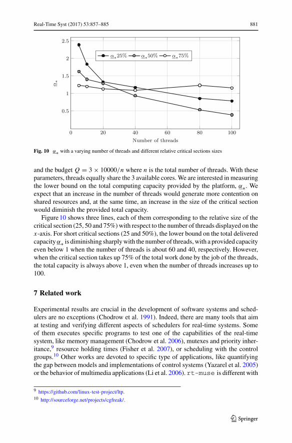
Fig. 10 α∗ with a varying number of threads and different relative critical sections sizes
and the budget Q = 3 × 10000/n where n is the total number of threads. With theseparameters, threads equally share the 3 available cores.We are interested in measuringthe lower bound on the total computing capacity provided by the platform, α∗. Weexpect that an increase in the number of threads would generate more contention onshared resources and, at the same time, an increase in the size of the critical sectionwould diminish the provided total capacity.
Figure10 shows three lines, each of them corresponding to the relative size of thecritical section (25, 50 and 75%)with respect to the number of threads displayed on thex-axis. For short critical sections (25 and 50%), the lower bound on the total deliveredcapacityα∗ is diminishing sharplywith the number of threads,with a provided capacityeven below 1 when the number of threads is about 60 and 40, respectively. However,when the critical section takes up 75% of the total work done by the job of the threads,the total capacity is always above 1, even when the number of threads increases up to100.
7 Related work
Experimental results are crucial in the development of software systems and sched-ulers are no exceptions (Chodrow et al. 1991). Indeed, there are many tools that aimat testing and verifying different aspects of schedulers for real-time systems. Someof them executes specific programs to test one of the capabilities of the real-timesystem, like memory management (Chodrow et al. 2006), mutexes and priority inher-itance,9 resource holding times (Fisher et al. 2007), or scheduling with the controlgroups.10 Other works are devoted to specific type of applications, like quantifyingthe gap between models and implementations of control systems (Yazarel et al. 2005)or the behavior of multimedia applications (Li et al. 2006). rt-muse is different with
9 https://github.com/linux-test-project/ltp.10 http://sourceforge.net/projects/cgfreak/.
123
882 Real-Time Syst (2017) 53:857–885
respect to both these classes, since it extracts performance metrics running a genericprogram, that represents the real application in its entirety. This is not the first workusing measurements from a real system to extract characteristics and models of dif-ferent aspects of the execution of a program on a particular architecture. A notableexample is (Baier et al. 2015), where the authors use measurement-based techniquesto fine-tune stochastic models that can be analyzed by a probabilistic model checker,applying the technique to the analysis of a test-and-set spinlock protocol (Anderson1990). Despite the similarity of performing tests on a real architecture to extract mod-els, the models and the aim of the two projects are complementary. The main ideaof (Baier et al. 2015) is to derive models from current architectures that could beextended to provide insight on the behavior of future platforms. However, it is quitecumbersome to obtain precise and reliable information about the operating systemsbehavior (Traeger et al. 2008). Due to this, we are satisfied with approximate compu-tation models and the generated upper and lower bounds.
Other tools like Hourglass (Regehr 2002) and rt-muse execute a specific work-load that could be specified as a command line parameter. Hourglass aims at testingthe behavior of schedulers for uniprocessor platforms. It computes a schedule for agiven workload, by executing the workload and recording which thread was runningand when context switches were happening. While rt-muse has in common withHourglass the execution of a workload that could be customized, rt-muse targetsmulticore platforms and provides experimental bounds to the amount of CPU providedin the given run. Since Hourglass provides a schedule, it is quite difficult to quantifythe results and understand if something could be improved in the implementation ofthe scheduler. One of the earliest tools for analyzing schedulers was the Hartstonebenchmark (Kamenoff and Weiderman 1991). Hartstone aims at testing the capabili-ties of a uniprocessor architecture by executing tests of increasing difficulty. In everyiteration, the pool of threads to be scheduled generates more load for the architectureand the number of iterations that could be executed without deadline misses deter-mines the benchmark score. While being extremely simple to implement in everyarchitecture, Hartstone lacks generality, since it assumes that threads do not interferewith each other, neither with shared memory nor with messages or similar. It also doesnot provide a clear interpretation of the results.
In an attempt to measure the effect of the most known sources of bottlenecksin production environments, lmbench (McVoy and Staelin 1996) provides a set ofmicrobenchmarks to test different performance issue sources in modern operating sys-tems. Similarly to rt-muse, it measures latencies and delays. However, the intentof lmbench is to reproduce problems and issues and not to benchmark the imple-mentation of real-time environments. The benchmark is not application-independent,nor it provides further analysis capabilities on the obtained result for the platform as awhole. A widely used real-time benchmark, cyclictest11 is a high-resolution analysistool to test a real-time system in its entirety, including the architecture, the schedulerand the workload. It measures the latency response of an application that only sleepsby continuously setting the instant in which the application should be woken up and
11 http://www.kernel.org/pub/linux/kernel/people/clrkwllms/rt-tests/.
123
Real-Time Syst (2017) 53:857–885 883
records the difference between this instant and the real wake up time. It is useful todetect unexpected large latencies on a system, for example due to overload condi-tions. This benchmark is very difficult to extend and does neither provide any insighton the behavior of the application in case its load is complex, nor combine differenttypes of operations. The suite of MiBench (Guthaus et al. 2001) is composed by 35applications that could be used in the context of embedded and real-time systems,for example in telecommunications or in the automotive domain. Despite it being acomplete workload, it does not provide any data analysis.
Bastoni et al. (2011) studied semi-partitioned schedulers in depth, evaluat-ing the scheduling overhead, the cache-induced delays and other metrics withLITMUSRT (Calandrino et al. 2006). While both rt-muse and (Bastoni et al. 2011)use traces of events to analyze the behavior of schedulers, LITMUSRT aims at sim-plifying the implementation of complex scheduling policies, while rt-muse aims atclosing the gap between theory and implementation by exposing the real-time char-acteristics of already implemented schedulers.
8 Conclusions and future work
To respond to the need of profiling the real-time behavior of real-time schedulers, weproposedrt-muse. Due to the extensible nature of the tool,we plan to implement newphaseswhich uses disk, network, or simply sleep. In addition, the results of the analysiscould be used to propose some patches in the Linux kernel, such as the introductionof more fairness when scheduling together SCHED_FIFO and SCHED_RR threads.
Acknowledgements The authors would like to thank Tommaso Cucinotta for his insightful comments onan earlier version of this draft.
Open Access This article is distributed under the terms of the Creative Commons Attribution 4.0 Interna-tional License (http://creativecommons.org/licenses/by/4.0/), which permits unrestricted use, distribution,and reproduction in any medium, provided you give appropriate credit to the original author(s) and thesource, provide a link to the Creative Commons license, and indicate if changes were made.
References
Abeni L, Buttazzo G (1998) Integrating multimedia applications in hard real-time systems. In: Proceedingsof the 19th IEEE real-time systems symposium, pp 4–13
Åkesson B, Goossens K (2011) Architectures andmodeling of predictable memory controllers for improvedsystem integration. In: Design, automation & test in europe conference & exhibition, pp 1–6
AlmeidaL, Pedreiras P, Fonseca JAG (2002) The FTT-CANprotocol:why and how. IEEETrans IndElectron49(6):1189–1201
Anderson JH, Srinivasan A (2001) Mixed Pfair/ERfair scheduling of asynchronous periodic tasks. In:Proceedings of the 13th Euromicro conference on real-time systems, pp 76–85
Anderson TE (1990) The performance of spin lock alternatives for shared-memory multiprocessors. IEEETrans Parallel Distrib Syst 1(1):6–16
Baccelli F, Cohen G, Olsder GJ, Quadrat JP (1992) Synchronization and linearity, vol 3. Wiley, New YorkBaier C, Daum M, Engel B, Härtig H, Klein J, Klüppelholz S, Märcker S, Tews H, Völp M (2015) Locks:
picking key methods for a scalable quantitative analysis. J Comput Syst Sci 81(1):258–287Bastoni A, Brandenburg BB, Anderson JH (2011) Is semi-partitioned scheduling practical? In: Proceedings
of the 2011 23rd Euromicro conference on real-time systems, pp 125–135
123
884 Real-Time Syst (2017) 53:857–885
Bini E, Bertogna M, Baruah S (2009) Virtual multiprocessor platforms: specification and use. In: Proceed-ings of the 2009 30th IEEE real-time systems symposium, pp 437–446
Brandenburg B, Anderson J (2007) Feather-trace: a light-weight event tracing toolkit. In: Proceedings ofthe third international workshop on operating systems platforms for embedded real-time applications,pp 19–28
Calandrino JM, Leontyev H, Block A, Devi UC, Anderson JH (2006) LitmusRT : a testbed for empiricallycomparing real-time multiprocessor schedulers. In: Proceedings of the 27th IEEE international real-time systems symposium, pp 111–126
Chodrow S, Jahanian F, Donner M (1991) Run-time monitoring of real-time systems. In: Proceedings ofthe 12th real-time systems symposium, pp 74–83
Cruz RL (1991) A calculus for network delay, part I: network elements in isolation. IEEE Trans Inf Theory37(1):114–131
Fisher N, Bertogna M, Baruah S (2007) Resource-locking durations in EDF-scheduled systems. In: Pro-ceedings of the 13th IEEE real time and embedded technology and applications symposium, pp 91–100
Guthaus MR, Ringenberg JS, Ernst D, Austin TM, Mudge T, Brown RB (2001) MiBench: a free, commer-cially representative embedded benchmark suite. In: 2001 IEEE internationalworkshoponproceedingsof the workload characterization. WWC-4, pp 3–14
Kamenoff N, Weiderman N (1991) Hartstone distributed benchmark: requirements and definitions. In:Proceedings of the twelfth real-time systems symposium, pp 199–208
Li ML, Van Achteren T, Brockmeyer E, Catthoor F (2006) Statistical performance analysis and estimationof coarse grain parallel multimedia processing system. In: Proceedings of the 12th IEEE real-time andembedded technology and applications symposium, pp 277–288
Lipari G, Bini E (2003) Resource partitioning among real-time applications. In: 15th Euromicro conferenceon real-time systems, pp 151–161
Maggio M, Lelli J, Bini E (2016) A tool for measuring supply functions of execution platforms. In: 2016IEEE 22nd international conference on embedded and real-time computing systems and applications(RTCSA), pp 39–48, Aug 2016
McVoy L, Staelin C (1996) LMBench: portable tools for performance analysis. In: Proceedings of the 1996annual conference on USENIX annual technical conference, pp 23–23
Mok AK, Feng X, Chen D (2001) Resource partition for real-time systems. In: Proceedings of the 7th IEEEreal-time technology and applications symposium, pp 75–84
Pellizzoni R, Bui BD, CaccamoM, Sha L (2008) Coscheduling of CPU and I/O transactions in COTS-basedembedded systems. In: Proceedings of the 2008 real-time systems symposium, pp 221–231
Pizlo F, Vitek J (2006) An emprical evaluation of memory management alternatives for real-time java. In:Proceedings of the 27th IEEE international real-time systems symposium, pp 35–46
Regehr J (2002) Inferring scheduling behavior with hourglass. In: Proceedings of the FREENIX track: 2002USENIX annual technical conference, pp 143–156
Regnier P, Lima G, Massa E, Levin G, Brandt S (2011) RUN: optimal multiprocessor real-time schedulingvia reduction to uniprocessor. In: Proceedings of the 32nd IEEE real-time systems symposium, pp104–115, Dec 2011
Shin I, Lee I (2003) Periodic resource model for compositional real-time guarantees. In: Proceedings of the24th IEEE international real-time systems symposium, pp 2–13
Thiele L, Chakraborty S, Naedele M (2000) Real-time calculus for scheduling hard real-time systems. In:Proceedings of the IEEE international symposium on circuits and systems, pp 101–104
TraegerA, ZadokE, JoukovN,Wright CP (2008)Anine year study of file system and storage benchmarking.Trans Storage 4(2):5:1–5:56
Xu M, Phan LT, Sokolsky O, Xi S, Lu C, Gill C, Lee I (2015) Cache-aware compositional analysis ofreal-time multicore virtualization platforms. Real Time Syst 51(6):675–723
Yazarel H, Girard A, Pappas GJ, Alur R (2005) Quantifying the gap between embedded control modelsand time-triggered implementations. In: Proceedings of the 26th IEEE international real-time systemssymposium, pp 111–120
Yun H, Yao G, Pellizzoni R, Caccamo M, Sha L (2016) Memory bandwidth management for efficientperformance isolation in multi-core platforms. IEEE Trans Comput 65(2):562–576
123
Real-Time Syst (2017) 53:857–885 885
Martina Maggio is an Associate Professor at the department ofAutomatic Control, Lund University. The focus of her PhD stud-ies at the Dipartimento di Elettronica e Informazione at Politecnicodi Milano, supervised by Alberto Leva, was the control-theoreticaldesign of computing systems components. For one year, she vis-ited the Computer Science and Artificial Intelligence Laboratory, atMassachusetts Institute of Technology, working under the supervi-sion of Anant Agarwal and together with Henry Hoffmann on theSelf-Aware Computing project, named one of ten “World ChangingIdeas” by Scientific American in 2011. During her stay at the LundUniversity, she worked with Karl-Erik Årzén on resource manage-ment in Real-Time computing systems and cloud computing prob-lems. Her research interests include the application of control the-ory to Software Engineering problems, with the goal of designingsoftware systems that provide predictable performance despite run-time variations.
Juri Lelli received a BS and a MS in Computer Engineering atthe University of Pisa (Italy). He then earned a PhD degree at theScuola Superiore Sant’Anna of Pisa, Italy (ReTiS Lab). He is oneof the original authors of the SCHED_DEADLINE scheduling pol-icy in Linux, and he is actively helping maintaining it. He is cur-rently working at ARM Ltd., where he continues contributing to theLinux scheduler development, with a special focus on energy awarescheduling and power management.
Enrico Bini is Associate Professor at Department of Computer Sci-ence, University of Turin. Until 2016, he was assistant professor atScuola Superiore Sant’Anna, Pisa. Also in 2012–14, he was Marie-Curie fellow at Lund University. In 2004, he completed the PhDon Real-Time Systems at Scuola Superiore Sant’Anna (recipientof the Spitali Award for best PhD thesis of the whole university).In January 2010 he also completed a Master degree in Mathe-matics with a thesis on optimal sampling for linear control sys-tems. He has published more than 90 papers (4 best-paper awards@RTNS @RTCSA @ICC) on real-time scheduling, operating sys-tems, optimization methods for real-time and control systems, opti-mal management of distributed and parallel resources. His serviceto the research community includes the participation in 58 Tech-nical Program Committees (including RTSS (2010, 2014, 2015,2017), RTAS (2009, 2010, 2011, 2013, 2015, 2016) and EMSOFT(2011, 2016)), the organization of 12 events (including PC co-Chair
of RTNS 2017, Local co-Organizer of ESWeek 2018), the review of 9 PhD thesis and about 40 papers/year, in the above mentioned research areas.
123