Rubidium 87 D Line Data - Daniel A. Stecksteck.us/alkalidata/rubidium87numbers.1.6.pdfRubidium 87 D Line Data Daniel A. Steck Theoretical Division (T-8), MS B285 Los Alamos National

Rubidium 87 D Line Data

Daniel A. SteckTheoretical Division (T-8), MS B285

Los Alamos National LaboratoryLos Alamos, NM 87545

25 September 2001(revision 1.6, 14 October 2003)

1 Introduction

In this reference we present many of the physical and optical properties of 87Rb that are relevant to variousquantum optics experiments. In particular, we give parameters that are useful in treating the mechanical effects oflight on 87Rb atoms. The measured numbers are given with their original references, and the calculated numbersare presented with an overview of their calculation along with references to more comprehensive discussions oftheir underlying theory. We also present a detailed discussion of the calculation of fluorescence scattering rates,because this topic is often not treated carefully in the literature.

The current version of this document is available at http://steck.us/alkalidata, along with “Cesium DLine Data” and “Sodium D Line Data.” Please send comments and corrections to [email protected].

2 87Rb Physical and Optical Properties

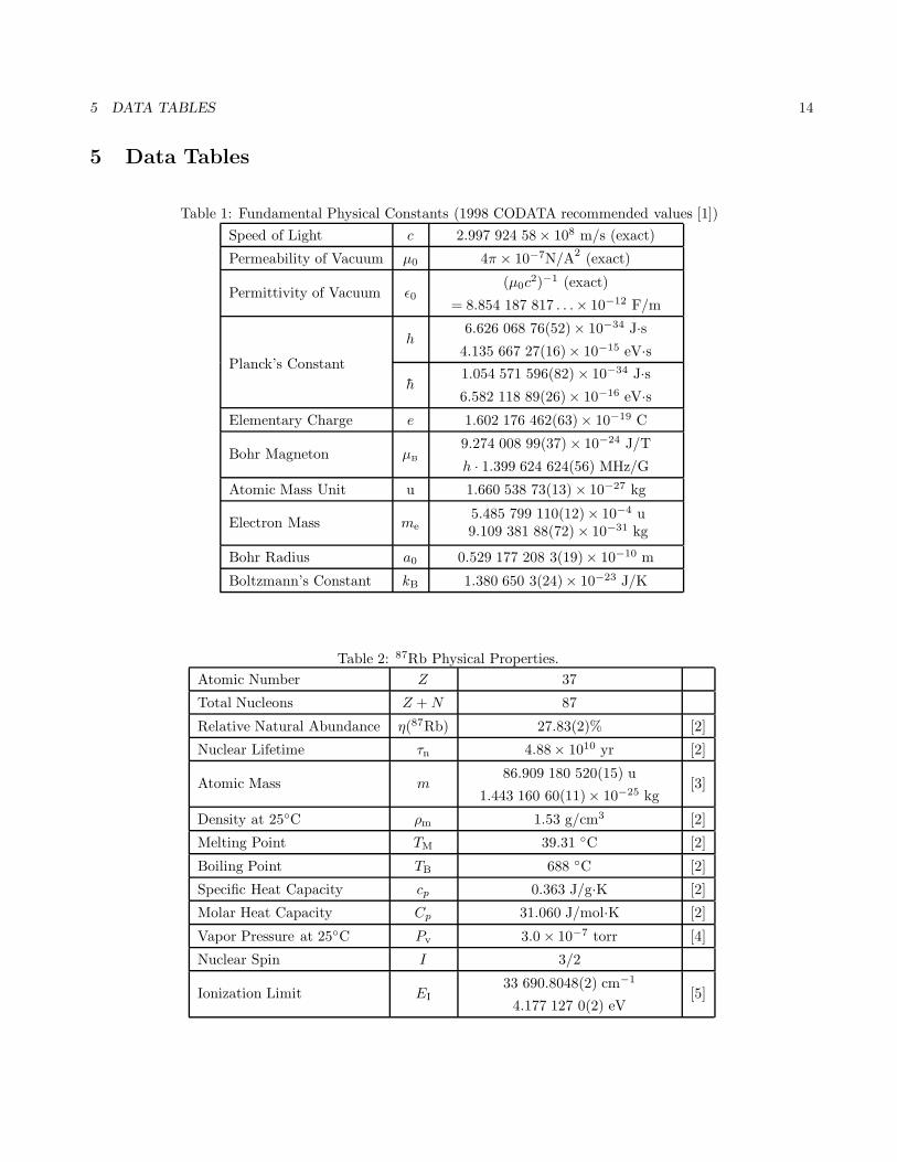
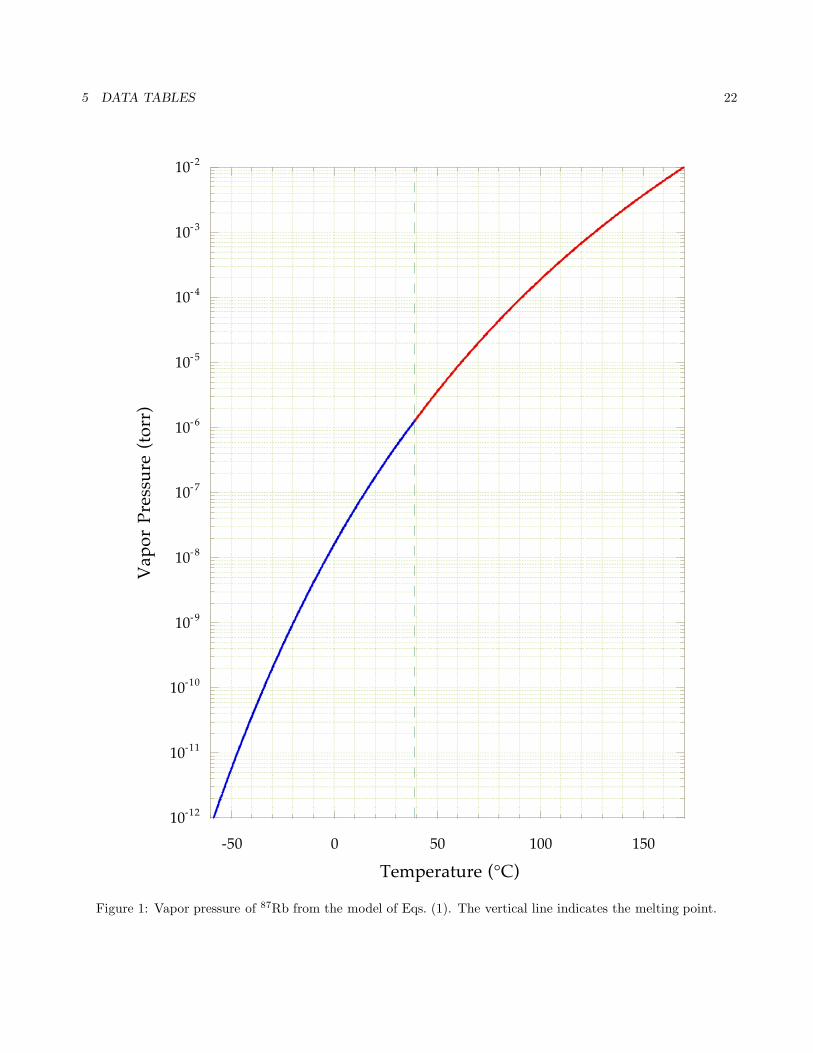
Some useful fundamental physical constants are given in Table 1. The values given are the 1998 CODATArecommended values, as listed in [1]. Some of the overall physical properties of 87Rb are given in Table 2. 87Rbhas 37 electrons, only one of which is in the outermost shell. 87Rb is not a stable isotope of rubidium, decayingto β− + 87Sr with a total disintegration energy of 0.283 MeV [2] (the only stable isotope is 85Rb), but has anextremely slow decay rate, thus making it effectively stable. This is the only isotope we consider in this reference.The mass is taken from the high-precision measurement of [3], and the density, melting point, boiling point, andheat capacities (for the naturally occurring form of Rb) are taken from [2]. The vapor pressure at 25C and thevapor pressure curve in Fig. 1 are taken from the vapor-pressure model given by [4], which is

log10 Pv = −94.048 26 − 1961.258T

− 0.037 716 87 T + 42.575 26 log10 T (solid phase)

log10 Pv = 15.882 53 − 4529.635T

+ 0.000 586 63 T − 2.991 38 log10 T (liquid phase),

(1)

where Pv is the vapor pressure in torr, and T is the temperature in K. This model should be viewed as a roughguide rather than a source of precise vapor-pressure values. The ionization limit is the minimum energy requiredto ionize a 87Rb atom; this value is taken from Ref. [5].

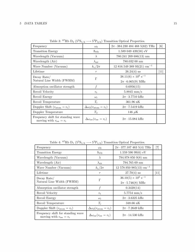
The optical properties of the 87Rb D line are given in Tables 3 and 4. The properties are given separatelyfor each of the two D-line components; the D2 line (the 52S1/2 −→ 52P3/2 transition) properties are given inTable 3, and the optical properties of the D1 line (the 52S1/2 −→ 52P1/2 transition) are given in Table 4. Of thesetwo components, the D2 transition is of much more relevance to current quantum and atom optics experiments,

http://steck.us/alkalidata

2 87RB PHYSICAL AND OPTICAL PROPERTIES 2

because it has a cycling transition that is used for cooling and trapping 87Rb. The frequencies ω0 of the D2 andD1 transitions were measured in [6] and [7], respectively (see also [8, 9] for more information on the D1 transitionmeasurement); the vacuum wavelengths λ and the wave numbers kL are then determined via the following relations:

λ =2πc

ω0kL =

2π

λ. (2)

The air wavelength λair = λ/n assumes index of refraction of n = 1.000 268 21, corresponding to dry air at apressure of 760 torr and a temperature of 22C. The index of refraction is calculated from the Edlen formula [10]:

nair = 1 +[(

8342.13 +2 406 030130 − κ2

+15 997

38.9− κ2

)×

(0.001 388 23 P

1 + 0.003 671 T

)− f

(5.722− 0.0457κ2

)]× 10−8 . (3)

Here, P is the air pressure in torr, T is the temperature in C, κ is the vacuum wave number kL/2π in µm−1, andf is the partial pressure of water vapor in the air, in torr. This formula is appropriate for laboratory conditionsand has an estimated uncertainty of ≤ 10−8.

The lifetimes are taken from a recent measurement employing beam-gas-laser spectroscopy [11]. Invertingthe lifetime gives the spontaneous decay rate Γ (Einstein A coefficient), which is also the natural (homogenous)line width (as an angular frequency) of the emitted radiation.

The spontaneous emission rate is a measure of the relative intensity of a spectral line. Commonly, the relativeintensity is reported as an absorption oscillator strength f , which is related to the decay rate by [12]

Γ =e2ω2

0

2πε0mec3

2J + 12J ′ + 1

f (4)

for a J −→ J ′ fine-structure transition, where me is the electron mass.The recoil velocity vr is the change in the 87Rb atomic velocity when absorbing or emitting a resonant photon,

and is given by

vr =hkL

m. (5)

The recoil energy hωr is defined as the kinetic energy of an atom moving with velocity v = vr, which is

hωr =h2k2

L

2m. (6)

The Doppler shift of an incident light field of frequency ωL due to motion of the atom is

∆ωd =vatom

cωL (7)

for small atomic velocities relative to c. For an atomic velocity vatom = vr, the Doppler shift is simply 2ωr. Finally,if one wishes to create a standing wave that is moving with respect to the lab frame, the two traveling-wavecomponents must have a frequency difference determined by the relation

vsw =∆ωsw

2π

λ

2, (8)

because ∆ωsw/2π is the beat frequency of the two waves, and λ/2 is the spatial periodicity of the standing wave.For a standing wave velocity of vr, Eq. (8) gives ∆ωsw = 4ωr. Two temperatures that are useful in cooling andtrapping experiments are also given here. The recoil temperature is the temperature corresponding to an ensemblewith a one-dimensional rms momentum of one photon recoil hkL:

Tr =h2k2

L

mkB

. (9)

3 HYPERFINE STRUCTURE 3

The Doppler temperature,

TD =hΓ2kB

, (10)

is the lowest temperature to which one expects to be able to cool two-level atoms in optical molasses, due to abalance of Doppler cooling and recoil heating [13]. Of course, in Zeeman-degenerate atoms, sub-Doppler coolingmechanisms permit temperatures substantially below this limit [14].

3 Hyperfine Structure

3.1 Energy Level Splittings

The 52S1/2 −→ 52P3/2 and 52S1/2 −→ 52P1/2 transitions are the components of a fine-structure doublet, and eachof these transitions additionally have hyperfine structure. The fine structure is a result of the coupling between theorbital angular momentum L of the outer electron and its spin angular momentum S. The total electron angularmomentum is then given by

J = L + S , (11)

and the corresponding quantum number J must lie in the range

|L − S| ≤ J ≤ L + S . (12)

(Here we use the convention that the magnitude of J is√

J(J + 1)h, and the eigenvalue of Jz is mJ h.) For theground state in 87Rb, L = 0 and S = 1/2, so J = 1/2; for the first excited state, L = 1, so J = 1/2 or J = 3/2.The energy of any particular level is shifted according to the value of J , so the L = 0 −→ L = 1 (D line) transitionis split into two components, the D1 line (52S1/2 −→ 52P1/2) and the D2 line (52S1/2 −→ 52P3/2). The meaningof the energy level labels is as follows: the first number is the principal quantum number of the outer electron, thesuperscript is 2S + 1, the letter refers to L (i.e., S ↔ L = 0, P ↔ L = 1, etc.), and the subscript gives the valueof J .

The hyperfine structure is a result of the coupling of J with the total nuclear angular momentum I. The totalatomic angular momentum F is then given by

F = J + I . (13)

As before, the magnitude of F can take the values

|J − I| ≤ F ≤ J + I . (14)

For the 87Rb ground state, J = 1/2 and I = 3/2, so F = 1 or F = 2. For the excited state of the D2 line (52P3/2),F can take any of the values 0, 1, 2, or 3, and for the D1 excited state (52P1/2), F is either 1 or 2. Again, theatomic energy levels are shifted according to the value of F .

Because the fine structure splitting in 87Rb is large enough to be resolved by many lasers (∼ 15 nm), thetwo D-line components are generally treated separately. The hyperfine splittings, however, are much smaller, andit is useful to have some formalism to describe the energy shifts. The Hamiltonian that describes the hyperfinestructure for each of the D-line components is [12, 15]

Hhfs = AhfsI · J + Bhfs

3(I · J)2 + 32I · J − I(I + 1)J(J + 1)

2I(2I − 1)J(2J − 1), (15)

which leads to a hyperfine energy shift of

∆Ehfs =12AhfsK + Bhfs

32K(K + 1) − 2I(I + 1)J(J + 1)

2I(2I − 1)2J(2J − 1), (16)

whereK = F (F + 1) − I(I + 1) − J(J + 1) , (17)


Ahfs is the magnetic dipole constant, and Bhfs is the electric quadrupole constant (although the term with Bhfs

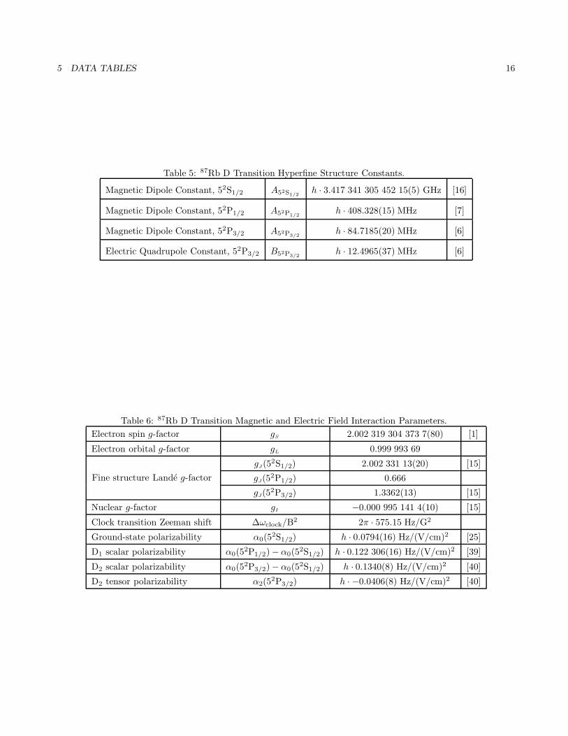
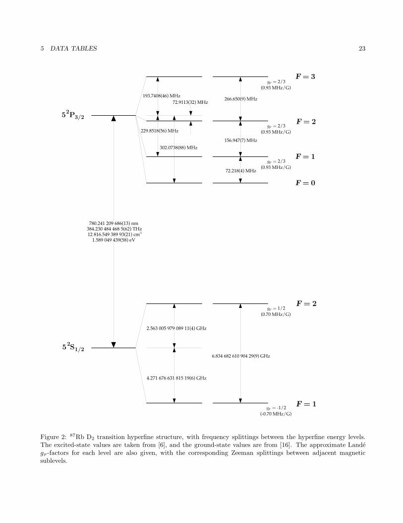
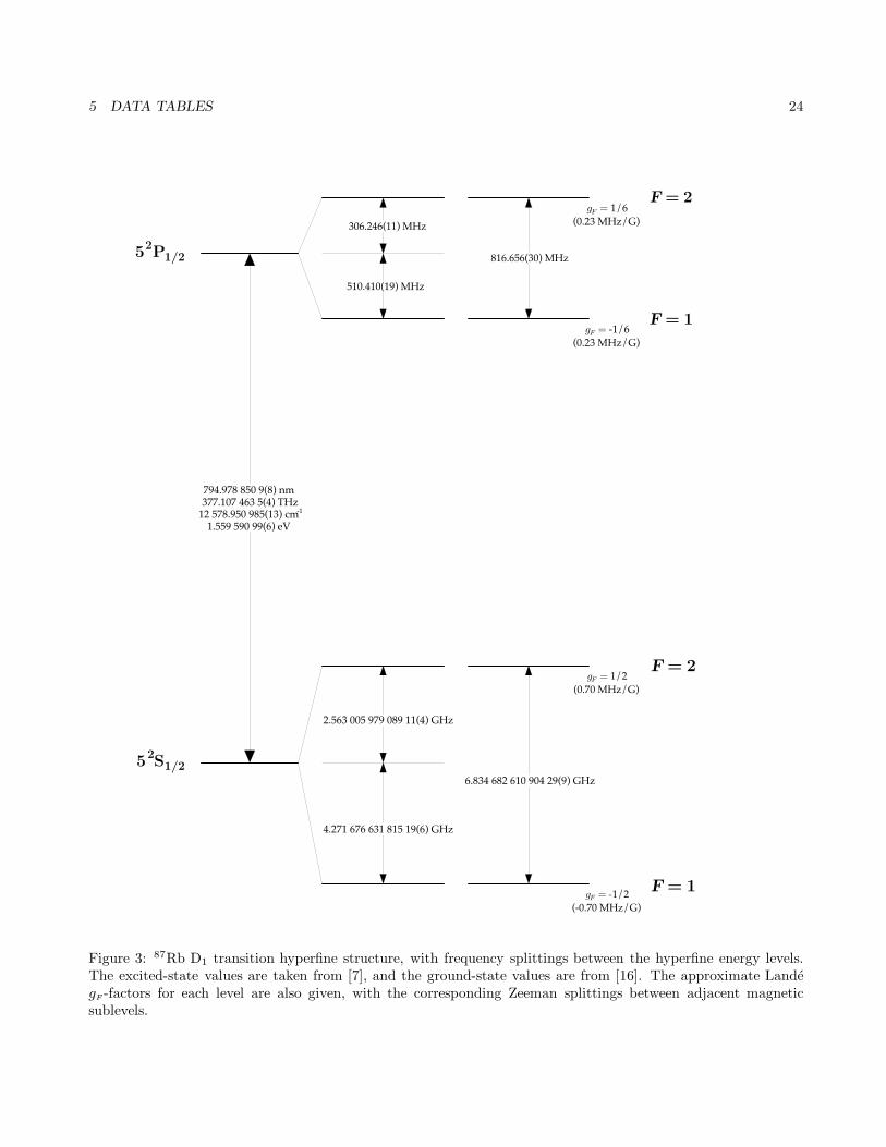
applies only to the excited manifold of the D2 transition and not to the levels with J = 1/2). These constants forthe 87Rb D line are listed in Table 5. The value for the ground state Ahfs constant is from a recent atomic-fountainmeasurement [16], while the constants listed for the 52P3/2 manifold were taken from a recent, precise measurement[6]. The Ahfs constant for the 52P1/2 manifold is taken from another recent measurement [7]. The energy shiftgiven by (16) is relative to the unshifted value (the “center of gravity”) listed in Table 3. The hyperfine structureof 87Rb, along with the energy splitting values, is diagrammed in Figs. 2 and 3.

3.2 Interaction with Static External Fields

3.2.1 Magnetic Fields

Each of the hyperfine (F ) energy levels contains 2F +1 magnetic sublevels that determine the angular distributionof the electron wave function. In the absence of external magnetic fields, these sublevels are degenerate. However,when an external magnetic field is applied, their degeneracy is broken. The Hamiltonian describing the atomicinteraction with the magnetic field is

HB =µB

h(gSS + gLL + gII) · B

=µB

h(gSSz + gLLz + gIIz)Bz ,

(18)

if we take the magnetic field to be along the z-direction (i.e., along the atomic quantization axis). In this Hamilto-nian, the quantities gS, gL, and gI are respectively the electron spin, electron orbital, and nuclear “g-factors” thataccount for various modifications to the corresponding magnetic dipole moments. The values for these factors arelisted in Table 6, with the sign convention of [15]. The value for gS has been measured very precisely, and thevalue given is the CODATA recommended value. The value for gL is approximately 1, but to account for the finitenuclear mass, the quoted value is given by

gL = 1 − me

mnuc, (19)

which is correct to lowest order in me/mnuc, where me is the electron mass and mnuc is the nuclear mass [17].The nuclear factor gI accounts for the entire complex structure of the nucleus, and so the quoted value is anexperimental measurement [15].

If the energy shift due to the magnetic field is small compared to the fine-structure splitting, then J is a goodquantum number and the interaction Hamiltonian can be written as

HB =µB

h(gJJz + gIIz)Bz . (20)

Here, the Lande factor gJ is given by [17]

gJ = gL

J(J + 1) − S(S + 1) + L(L + 1)2J(J + 1)

+ gS

J(J + 1) + S(S + 1) − L(L + 1)2J(J + 1)

1 +J(J + 1) + S(S + 1) − L(L + 1)

2J(J + 1),

(21)

where the second, approximate expression comes from taking the approximate values gS 2 and gL 1. Theexpression here does not include corrections due to the complicated multielectron structure of 87Rb [17] and QEDeffects [18], so the values of gJ given in Table 6 are experimental measurements [15] (except for the 52P1/2 statevalue, for which there has apparently been no experimental measurement).

If the energy shift due to the magnetic field is small compared to the hyperfine splittings, then similarly F isa good quantum number, so the interaction Hamiltonian becomes [19]

HB = µB gF Fz Bz , (22)


where the hyperfine Lande g-factor is given by

gF = gJ

F (F + 1) − I(I + 1) + J(J + 1)2F (F + 1)

+ gI

F (F + 1) + I(I + 1) − J(J + 1)2F (F + 1)

gJ

F (F + 1) − I(I + 1) + J(J + 1)2F (F + 1)

.

(23)

The second, approximate expression here neglects the nuclear term, which is a correction at the level of 0.1%,since gI is much smaller than gJ .

For weak magnetic fields, the interaction Hamiltonian HB perturbs the zero-field eigenstates of Hhfs. To lowestorder, the levels split linearly according to [12]

∆E|F mF 〉 = µB gF mF Bz . (24)

The approximate gF factors computed from Eq. (23) and the corresponding splittings between adjacent magneticsublevels are given in Figs. 2 and 3. The splitting in this regime is called the anomalous Zeeman effect.

For strong fields where the appropriate interaction is described by Eq. (20), the interaction term dominatesthe hyperfine energies, so that the hyperfine Hamiltonian perturbs the strong-field eigenstates |J mJ I mI〉. Theenergies are then given to lowest order by [20]

E|J mJ I mI〉 = AhfsmJmI + Bhfs

3(mJmI )2 + 32mJmI − I(I + 1)J(J + 1)

2J(2J − 1)I(2I − 1)+ µB(gJ mJ + gI mI)Bz . (25)

The energy shift in this regime is called the Paschen-Back effect.For intermediate fields, the energy shift is more difficult to calculate, and in general one must numerically

diagonalize Hhfs + HB. A notable exception is the Breit-Rabi formula [12, 19, 21], which applies to the ground-state manifold of the D transition:

E|J=1/2 mJ I mI〉 = − ∆Ehfs

2(2I + 1)+ gI µB mB ± ∆Ehfs

2

(1 +

4mx

2I + 1+ x2

)1/2

. (26)

In this formula, ∆Ehfs = Ahfs(I + 1/2) is the hyperfine splitting, m = mI ± mJ = mI ± 1/2 (where the ± sign istaken to be the same as in (26)), and

x =(gJ − gI)µB B

∆Ehfs. (27)

In order to avoid a sign ambiguity in evaluating (26), the more direct formula

E|J=1/2 mJ I mI〉 = ∆EhfsI

2I + 1± 1

2(gJ + 2IgI)µB B (28)

can be used for the two states m = ±(I + 1/2). The Breit-Rabi formula is useful in finding the small-field shift ofthe “clock transition” between the mF = 0 sublevels of the two hyperfine ground states, which has no first-orderZeeman shift. Using m = mF for small magnetic fields, we obtain

∆ωclock =(gJ − gI)2µ2

B

2h∆EhfsB2 (29)

to second order in the field strength.If the magnetic field is sufficiently strong that the hyperfine Hamiltonian is negligible compared to the inter-

action Hamiltonian, then the effect is termed the normal Zeeman effect for hyperfine structure. For even strongerfields, there are Paschen-Back and normal Zeeman regimes for the fine structure, where states with different J canmix, and the appropriate form of the interaction energy is Eq. (18). Yet stronger fields induce other behaviors,such as the quadratic Zeeman effect [19], which are beyond the scope of the present discussion.

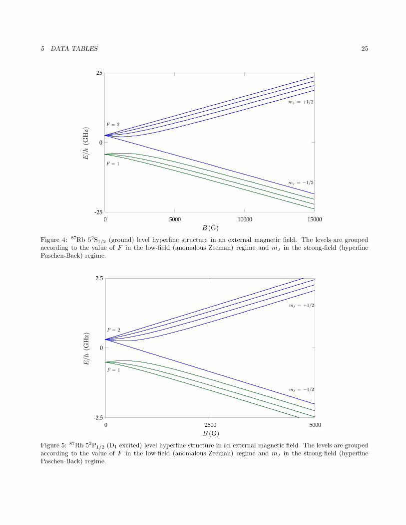
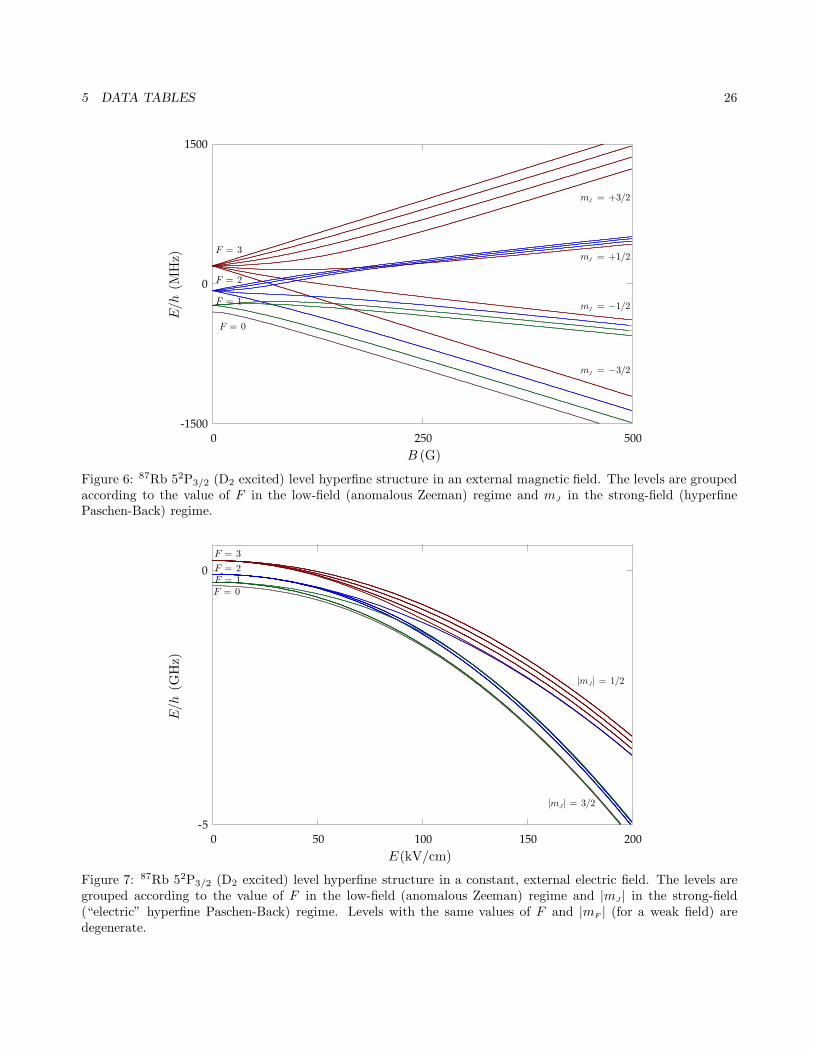
The level structure of 87Rb in the presence of a magnetic field is shown in Figs. 4-6 in the weak-field (anomalousZeeman) regime through the hyperfine Paschen-Back regime.


3.2.2 Electric Fields

An analogous effect, the dc Stark effect, occurs in the presence of a static external electric field. The interactionHamiltonian in this case is [22–24]

HE = −12α0E

2z − 1

2α2E

2z

3J2z − J(J + 1)J(2J − 1)

, (30)

where we have taken the electric field to be along the z-direction, α0 and α2 are respectively termed the scalarand tensor polarizabilities, and the second (α2) term is nonvanishing only for the J = 3/2 level. The first termshifts all the sublevels with a given J together, so that the Stark shift for the J = 1/2 states is trivial. Theonly mechanism for breaking the degeneracy of the hyperfine sublevels in (30) is the Jz contribution in the tensorterm. This interaction splits the sublevels such that sublevels with the same value of |mF | remain degenerate.An expression for the hyperfine Stark shift, assuming a weak enough field that the shift is small compared to thehyperfine splittings, is [22]

∆E|J I F mF 〉 = −12α0E

2z − 1

2α2E

2z

[3m2F− F (F + 1)][3X(X − 1) − 4F (F + 1)J(J + 1)]

(2F + 3)(2F + 2)F (2F − 1)J(2J − 1), (31)

whereX = F (F + 1) + J(J + 1) − I(I + 1) . (32)

For stronger fields, when the Stark interaction Hamiltonian dominates the hyperfine splittings, the levels splitaccording to the value of |mJ |, leading to an electric-field analog to the Paschen-Back effect for magnetic fields.

The static polarizability is also useful in the context of optical traps that are very far off resonance (i.e., severalto many nm away from resonance, where the rotating-wave approximation is invalid), since the optical potential isgiven in terms of the ground-state polarizability as V = −1/2α0E

2, where E is the amplitude of the optical field.A more accurate expression for the far-off resonant potential arises by replacing the static polarizability with thefrequency-dependent polarizability [25]

α0(ω) =ω 2

0 α0

ω 20 − ω2

, (33)

where ω0 is the resonant frequency of the lowest-energy transition (i.e., the D1 resonance); this approximateexpression is valid for light tuned far to the red of the D1 line.

The 87Rb polarizabilities are tabulated in Table 6. Notice that the differences in the excited state and groundstate scalar polarizabilities are given, rather than the excited state polarizabilities, since these are the quantitiesthat were actually measured experimentally. The polarizabilities given here are in SI units, although they areoften given in cgs units (units of cm3) or atomic units (units of a3

0, where the Bohr radius a0 is given in Table 1).The SI values can be converted to cgs units via α[cm3] = 5.95531× 10−22 α[Hz/(V/cm)2] [25], and subsequentlythe conversion to atomic units is straightforward.

The level structure of 87Rb in the presence of an external dc electric field is shown in Fig. 7 in the weak-fieldregime through the electric hyperfine Paschen-Back regime.

3.3 Reduction of the Dipole Operator

The strength of the interaction between 87Rb and nearly-resonant optical radiation is characterized by the dipolematrix elements. Specifically, 〈F mF |er|F ′ m′

F〉 denotes the matrix element that couples the two hyperfine

sublevels |F mF 〉 and |F ′ m′F〉 (where the primed variables refer to the excited states and the unprimed variables

refer to the ground states). To calculate these matrix elements, it is useful to factor out the angular dependenceand write the matrix element as a product of a Clebsch-Gordan coefficient and a reduced matrix element, usingthe Wigner-Eckart theorem [26]:

〈F mF |erq|F ′ m′F 〉 = 〈F ‖er‖F ′〉〈F mF |F ′ 1 m′

F q〉 . (34)

4 RESONANCE FLUORESCENCE 7

Here, q is an index labeling the component of r in the spherical basis, and the doubled bars indicate that thematrix element is reduced. We can also write (34) in terms of a Wigner 3-j symbol as

〈F mF |erq|F ′ m′F 〉 = 〈F ‖er‖F ′〉(−1)F ′−1+mF

√2F + 1

(F ′ 1 Fm′

F q −mF

). (35)

Notice that the 3-j symbol (or, equivalently, the Clebsch-Gordan coefficient) vanishes unless the sublevels satisfymF = m′

F + q. This reduced matrix element can be further simplified by factoring out the F and F ′ dependenceinto a Wigner 6-j symbol, leaving a further reduced matrix element that depends only on the L, S, and J quantumnumbers [26]:

〈F ‖er‖F ′〉 ≡ 〈J I F ‖er‖J ′ I′ F ′〉= 〈J‖er‖J ′〉(−1)F ′+J+1+I

√(2F ′ + 1)(2J + 1)

J J ′ 1F ′ F I

.

(36)

Again, this new matrix element can be further factored into another 6-j symbol and a reduced matrix elementinvolving only the L quantum number:

〈J‖er‖J ′〉 ≡ 〈L S J‖er‖L′ S′ J ′〉= 〈L‖er‖L′〉(−1)J′+L+1+S

√(2J ′ + 1)(2L + 1)

L L′ 1J ′ J S

.

(37)

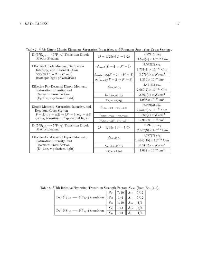
The numerical value of the 〈J = 1/2‖er‖J ′ = 3/2〉 (D2) and the 〈J = 1/2‖er‖J ′ = 1/2〉 (D1) matrix elements aregiven in Table 7. These values were calculated from the lifetime via the expression [27]

1τ

=ω3

0

3πε0hc3

2J + 12J ′ + 1

|〈J‖er‖J ′〉|2 . (38)

Note that all the equations we have presented here assume the normalization convention∑M ′

|〈J M |er|J ′ M ′〉|2 =∑M ′q

|〈J M |erq|J ′ M ′〉|2 = |〈J‖er‖J ′〉|2 . (39)

There is, however, another common convention (used in Ref. [28]) that is related to the convention used hereby (J‖er‖J ′) =

√2J + 1 〈J‖er‖J ′〉. Also, we have used the standard phase convention for the Clebsch-Gordan

coefficients as given in Ref. [26], where formulae for the computation of the Wigner 3-j (equivalently, Clebsch-Gordan) and 6-j (equivalently, Racah) coefficients may also be found.

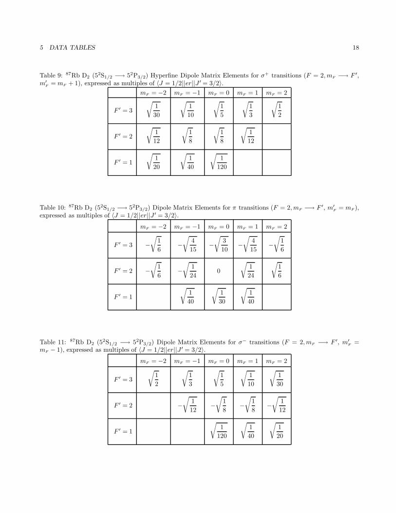
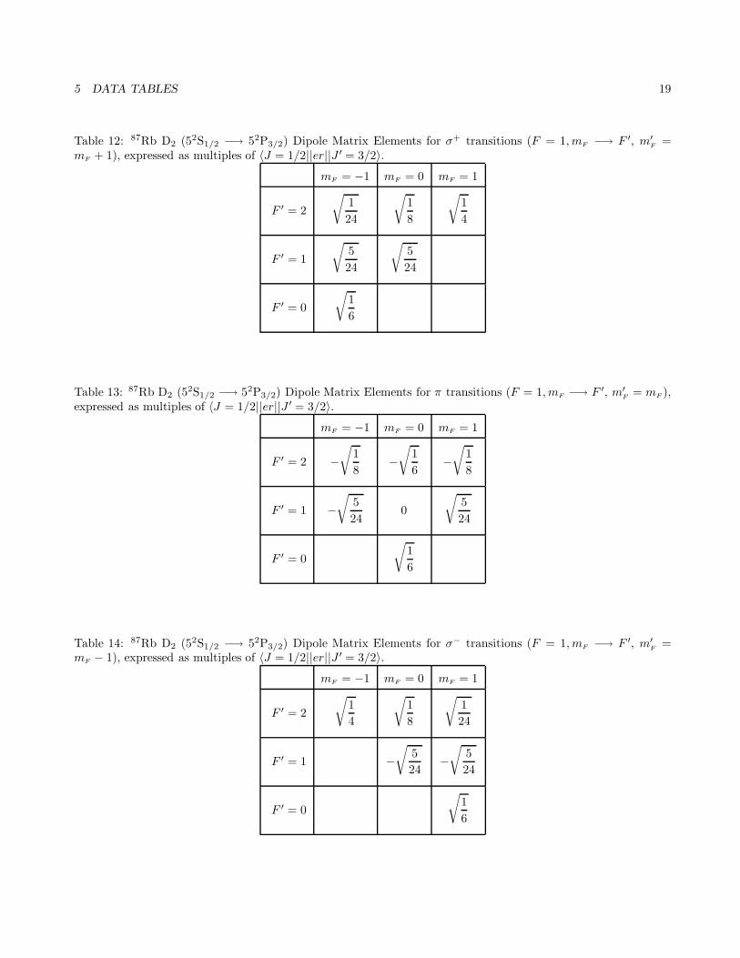
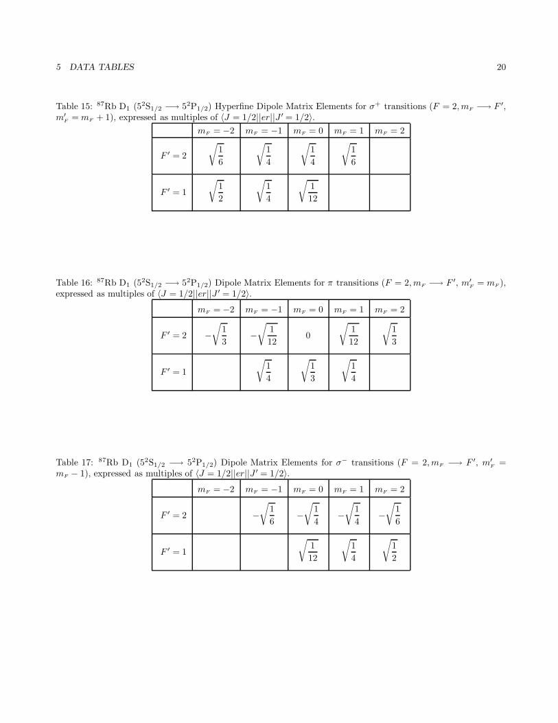
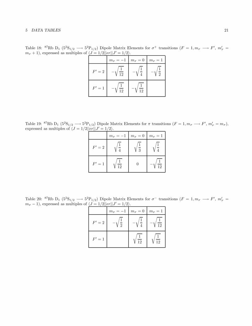
The dipole matrix elements for specific |F mF 〉 −→ |F ′ m′F 〉 transitions are listed in Tables 9-20 as multiples of

〈J‖er‖J ′〉. The tables are separated by the ground-state F number and the polarization of the transition (whereσ+-polarized light couples mF −→ m′

F= mF + 1, π-polarized light couples mF −→ m′

F= mF , and σ−-polarized

light couples mF −→ m′F = mF − 1).

4 Resonance Fluorescence

4.1 Symmetries of the Dipole Operator

Although the hyperfine structure of 87Rb is quite complicated, it is possible to take advantage of some symmetriesof the dipole operator in order to obtain relatively simple expressions for the photon scattering rates due toresonance fluorescence. In the spirit of treating the D1 and D2 lines separately, we will discuss the symmetries inthis section implicitly assuming that the light is interacting with only one of the fine-structure components at atime. First, notice that the matrix elements that couple to any single excited state sublevel |F ′ m′

F 〉 add up to afactor that is independent of the particular sublevel chosen,

∑q F

|〈F (m′F + q)|erq|F ′ m′

F 〉|2 =2J + 12J ′ + 1

|〈J‖er‖J ′〉|2 , (40)


as can be verified from the dipole matrix element tables. The degeneracy-ratio factor of (2J +1)/(2J ′ +1) (whichis 1 for the D1 line or 1/2 for the D2 line) is the same factor that appears in Eq. (38), and is a consequence of thenormalization convention (39). The interpretation of this symmetry is simply that all the excited state sublevelsdecay at the same rate Γ, and the decaying population “branches” into various ground state sublevels.

Another symmetry arises from summing the matrix elements from a single ground-state sublevel to the levelsin a particular F ′ energy level:

SFF ′ :=∑

q

(2F ′ + 1)(2J + 1)

J J ′ 1F ′ F I

2

|〈F mF |F ′ 1 (mF − q) q〉|2

= (2F ′ + 1)(2J + 1)

J J ′ 1F ′ F I

2

.

(41)

This sum SFF ′ is independent of the particular ground state sublevel chosen, and also obeys the sum rule∑F ′

SFF ′ = 1. (42)

The interpretation of this symmetry is that for an isotropic pump field (i.e., a pumping field with equal componentsin all three possible polarizations), the coupling to the atom is independent of how the population is distributedamong the sublevels. These factors SFF ′ (which are listed in Table 8) provide a measure of the relative strengthof each of the F −→ F ′ transitions. In the case where the incident light is isotropic and couples two of the Flevels, the atom can be treated as a two-level atom, with an effective dipole moment given by

|diso,eff(F −→ F ′)|2 =13SFF ′ |〈J ||er||J ′〉|2 . (43)

The factor of 1/3 in this expression comes from the fact that any given polarization of the field only interacts withone (of three) components of the dipole moment, so that it is appropriate to average over the couplings ratherthan sum over the couplings as in (41).

When the light is detuned far from the atomic resonance (∆ Γ), the light interacts with several hyperfinelevels. If the detuning is large compared to the excited-state frequency splittings, then the appropriate dipolestrength comes from choosing any ground state sublevel |F mF 〉 and summing over its couplings to the excitedstates. In the case of π-polarized light, the sum is independent of the particular sublevel chosen:

∑F ′

(2F ′ + 1)(2J + 1)

J J ′ 1F ′ F I

2

|〈F mF |F ′ 1 mF 0〉|2 =13

. (44)

This sum leads to an effective dipole moment for far detuned radiation given by

|ddet,eff|2 =13|〈J ||er||J ′〉|2 . (45)

The interpretation of this factor is also straightforward. Because the radiation is far detuned, it interacts withthe full J −→ J ′ transition; however, because the light is linearly polarized, it interacts with only one componentof the dipole operator. Then, because of spherical symmetry, |d|2 ≡ |er|2 = e2(|x|2 + |y|2 + |z|2) = 3e2|z|2. Notethat this factor of 1/3 also appears for σ± light, but only when the sublevels are uniformly populated (which, ofcourse, is not the equilibrium configuration for these polarizations). The effective dipole moments for this caseand the case of isotropic pumping are given in Table 7.

4.2 Resonance Fluorescence in a Two-Level Atom


In these two cases, where we have an effective dipole moment, the atoms behave like simple two-level atoms. Atwo-level atom interacting with a monochromatic field is described by the optical Bloch equations [27],

ρgg =iΩ2

(ρge − ρeg) + Γρee

ρee = − iΩ2

(ρge − ρeg) − Γρee

˙ρge = −(γ + i∆)ρge −iΩ2

(ρee − ρgg) ,

(46)

where the ρij are the matrix elements of the density operator ρ := |ψ〉〈ψ|, Ω := −d ·E0/h is the resonant Rabifrequency, d is the dipole operator, E0 is the electric field amplitude (E = E0 cos ωLt), ∆ := ωL − ω0 is thedetuning of the laser field from the atomic resonance, Γ = 1/τ is the natural decay rate of the excited state,γ := Γ/2 + γc is the “transverse” decay rate (where γc is a phenomenological decay rate that models collisions),ρge := ρge exp(−i∆t) is a “slowly varying coherence,” and ρge = ρ∗eg. In writing down these equations, we havemade the rotating-wave approximation and used a master-equation approach to model spontaneous emission.Additionally, we have ignored any effects due to the motion of the atom and decays or couplings to other auxiliarystates. In the case of purely radiative damping (γ = Γ/2), the excited state population settles to the steady statesolution

ρee(t → ∞) =(Ω/Γ)2

1 + 4 (∆/Γ)2 + 2 (Ω/Γ)2. (47)

The (steady state) total photon scattering rate (integrated over all directions and frequencies) is then given byΓρee(t → ∞):

Rsc =(

Γ2

)(I/Isat)

1 + 4 (∆/Γ)2 + (I/Isat). (48)

In writing down this expression, we have defined the saturation intensity Isat such that

I

Isat= 2

(ΩΓ

)2

, (49)

which gives (with I = (1/2)cε0E 20 )

Isat =cε0Γ2h2

4|ε · d|2 , (50)

where ε is the unit polarization vector of the light field, and d is the atomic dipole moment. With Isat definedin this way, the on-resonance scattering cross section σ, which is proportional to Rsc(∆ = 0)/I, drops to 1/2 ofits weakly pumped value σ0 when I = Isat. More precisely, we can define the scattering cross section σ as thepower radiated by the atom divided by the incident energy flux (i.e., so that the scattered power is σI), whichfrom Eq. (48) becomes

σ =σ0

1 + 4 (∆/Γ)2 + (I/Isat), (51)

where the on-resonance cross section is defined by

σ0 =hωΓ2Isat

. (52)

Additionally, the saturation intensity (and thus the scattering cross section) depends on the polarization of thepumping light as well as the atomic alignment, although the smallest saturation intensity (Isat(mF =±2 →m′

F=±3),

discussed below) is often quoted as a representative value. Some saturation intensities and scattering cross sectionscorresponding to the discussions in Section 4.1 are given in Table 7. A more detailed discussion of the resonancefluorescence from a two-level atom, including the spectral distribution of the emitted radiation, can be found inRef. [27].


4.3 Optical Pumping

If none of the special situations in Section 4.1 applies to the fluorescence problem of interest, then the effects ofoptical pumping must be accounted for. A discussion of the effects of optical pumping in an atomic vapor on thesaturation intensity using a rate-equation approach can be found in Ref. [29]. Here, however, we will carry out ananalysis based on the generalization of the optical Bloch equations (46) to the degenerate level structure of alkaliatoms. The appropriate master equation for the density matrix of a Fg → Fe hyperfine transition is [30–33]

∂

∂tρα mα, β mβ = − i

2

⎡⎣δαe

∑mg

Ω(mα, mg) ρg mg, β mβ − δgβ

∑me

Ω(me, mβ) ρα mα , e me

+ δαg

∑me

Ω∗(me, mα) ρe me, β mβ − δeβ

∑mg

Ω∗(mβ , mg) ρα mα , g mg

⎤⎦

⎫⎪⎪⎪⎪⎪⎪⎬⎪⎪⎪⎪⎪⎪⎭

(pump field)

− δαeδeβ Γ ρα mα, β mβ

− δαeδgβΓ2

ρα mα, β mβ

− δαgδeβΓ2

ρα mα, β mβ

+ δαgδgβ Γ1∑

q=−1

[ρe (mα+q), e (mβ+q)

〈Fe (mα + q)|Fg 1 mα q〉〈Fe (mβ + q)|Fg 1 mβ q〉]

⎫⎪⎪⎪⎪⎪⎪⎪⎪⎪⎪⎪⎪⎪⎪⎪⎬⎪⎪⎪⎪⎪⎪⎪⎪⎪⎪⎪⎪⎪⎪⎪⎭

(dissipation)

+ i(δαeδgβ − δαgδeβ) ∆ ρα mα , β mβ

(free evolution)

(53)where

Ω(me, mg) = 〈Fg mg |Fe 1 me − (me − mg)〉 Ω−(me−mg)

= (−1)Fe−Fg+me−mg

√2Fg + 12Fe + 1

〈Fe me|Fg 1 mg (me − mg)〉 Ω−(me−mg)

(54)

is the Rabi frequency between two magnetic sublevels,

Ωq =2〈Fe||er||Fg〉E(+)

q

h(55)

is the overall Rabi frequency with polarization q (E(+)q is the field amplitude associated with the positive-rotating

component, with polarization q in the spherical basis), and δ is the Kronecker delta symbol. This master equationignores coupling to F levels other than the ground (g) and excited (e) levels; hence, this equation is appropriatefor a cycling transition such as F = 2 −→ F ′ = 3. Additionally, this master equation assumes purely radiativedamping and, as before, does not describe the motion of the atom.

To calculate the scattering rate from a Zeeman-degenerate atom, it is necessary to solve the master equationfor the steady-state populations. Then, the total scattering rate is given by

Rsc = ΓPe = Γ∑me

ρe me, e me , (56)

where Pe is the total population in the excited state. In addition, by including the branching ratios of thespontaneous decay, it is possible to account for the polarization of the emitted radiation. Defining the scattering


rate Rsc, −q for the polarization (−q), we have

Rsc, −q =∑

me mg

|〈Fe me|Fg 1 mg q〉|2ρe me, e me , (57)

where, as before, the only nonzero Clebsch-Gordan coefficients occur for me = mg + q. As we have defined ithere, q = ±1 corresponds to σ±-polarized radiation, and q = 0 corresponds to π-polarized radiation. The angulardistribution for the σ± scattered light is simply the classical radiation pattern for a rotating dipole,

f ±sc (θ, φ) =

316π

(1 + cos2 θ) , (58)

and the angular distribution for the π-scattered light is the classical radiation pattern for an oscillating dipole,

f 0sc(θ, φ) =

38π

sin2 θ . (59)

The net angular pattern will result from the interference of these three distributions.In general, this master equation is difficult to treat analytically, and even a numerical solution of the time-

dependent equations can be time-consuming if a large number of degenerate states are involved. In the followingdiscussions, we will only consider some simple light configurations interacting with the F = 2 −→ F ′ = 3 cyclingtransition that can be treated analytically. Discussions of Zeeman-degenerate atoms and their spectra can befound in Refs. [33–37].

4.3.1 Circularly (σ±) Polarized Light

The cases where the atom is driven by either σ+ or σ− light (i.e. circularly polarized light with the atomicquantization axis aligned with the light propagation direction) are straightforward to analyze. In these cases, thelight transfers its angular momentum to the atom, and thus the atomic population is transferred to the state withthe largest corresponding angular momentum. In the case of the F = 2 −→ F ′ = 3 cycling transition, a σ+ drivingfield will transfer all the atomic population into the |F = 2, mF = 2〉 −→ |F ′ = 3, m′

F= 3〉 cycling transition,

and a σ− driving field will transfer all the population into the |F = 2, mF = −2〉 −→ |F ′ = 3, m′F = −3〉 cycling

transition. In both cases, the dipole moment,

d(mF =±2 →mF =±3) =2J + 12J ′ + 1

|〈J = 1/2‖er‖J ′ = 3/2〉|2 , (60)

is given in Table 7. Also, in this case, the saturation intensity reduces to

Isat =hω3Γ12πc2

, (61)

and the scattering cross section reduces to

σ0 =3λ2

2π. (62)

Note that these values are only valid in steady state. If the pumping field is weak, the “settling time” of the atomto its steady state can be long, resulting in a time-dependent effective dipole moment (and saturation intensity).For example, beginning with a uniform sublevel population in the F = 2 ground level, the saturation intensity willbegin at 3.58 mW/cm2 and equilibrate at 1.67 mW/cm2 for a circularly polarized pump. Also, if there are any“remixing” effects such as collisions or magnetic fields not aligned with the axis of quantization, the system maycome to equilibrium in some other configuration.


4.3.2 Linearly (π) Polarized Light

If the light is π-polarized (linearly polarized along the quantization axis), the equilibrium population distributionis more complicated. In this case, the atoms tend to accumulate in the sublevels near m = 0. Gao [33] has derivedanalytic expressions for the equilibrium populations of each sublevel and showed that the equilibrium excited-statepopulation is given by Eq. (47) if Ω2 is replaced by

gP(2Fg + 1)|Ω0|2 , (63)

where Ω0 is the only nonzero component of the Rabi-frequency vector (calculated with respect to the reduced dipolemoment |〈F ||er||F ′〉|2 = SFF ′ |〈J ||er||J ′〉|2), and gP is a (constant) geometric factor that accounts for the opticalpumping. For the 87Rb F = 2 −→ F ′ = 3 cycling transition, this factor has the value gP = 36/461 ≈ 0.07809,leading to a steady-state saturation intensity of Isat = 3.05 mW/cm2.

4.3.3 One-Dimensional σ+ − σ− Optical Molasses

We now consider the important case of an optical molasses in one dimension formed by one σ+ and one σ−

field (e.g., by two right-circularly polarized, counterpropagating laser fields). These fields interfere to form afield that is linearly polarized, where the polarization vector traces out a helix in space. Because the light islinearly polarized everywhere, and the steady-state populations are independent of the polarization direction (inthe plane orthogonal to the axis of quantization), the analysis of the previous section applies. When we applythe formula (48) to calculate the scattering rate, then, we simply use the saturation intensity calculated in theprevious section, and use the total intensity (twice the single-beam intensity) for I in the formula. Of course,this steady-state treatment is only strictly valid for a stationary atom, since a moving atom will see a changingpolarization and will thus be slightly out of equilibrium, leading to sub-Doppler cooling mechanism [14].

4.3.4 Three-Dimensional Optical Molasses

Finally, we consider an optical molasses in three dimensions, composed of six circularly polarized beams. Thisoptical configuration is found in the commonly used six-beam magneto-optic trap (MOT). However, as we shall see,this optical configuration is quite complicated, and we will only be able to estimate the total rate of fluorescence.

First, we will derive an expression for the electric field and intensity of the light. A typical MOT is formed withtwo counterpropagating, right-circularly polarized beams along the z-axis and two pairs of counterpropagating,left-circularly polarized beams along the x- and y-axes. Thus, the net electric field is given by

E(r, t) =E0

2e−iωt

[eikz

(x − iy√

2

)+ e−ikz

(x + iy√

2

)

+ eikx

(y + iz√

2

)+ e−ikx

(y − iz√

2

)+ eiky

(z + ix√

2

)+ e−iky

(z − ix√

2

)]+ c.c.

=√

2E0e−iωt

[(cos kz − sin ky)x + (sin kz + cos kx)y + (cos ky − sinkx)z

].

(64)

The polarization is linear everywhere for this choice of phases, but the orientation of the polarization vector isstrongly position-dependent. The corresponding intensity is given by

I(r) = I0

[6 − 4(cos kz sin ky + cos ky sin kx − sinkz cos kx)

], (65)

where I0 := (1/2)cε0E 20 is the intensity of a single beam. The six beams form an intensity lattice in space, with

an average intensity of 6I0 and a discrete set of points with zero intensity. Note, however, that the form of thisinterference pattern is specific to the set of phases chosen here, since there are more than the minimal number ofbeams needed to determine the lattice pattern.


It is clear that this situation is quite complicated, because an atom moving in this molasses will experience botha changing intensity and polarization direction. The situation becomes even more complicated when the magneticfield gradient from the MOT is taken into account. However, we can estimate the scattering rate if we ignore themagnetic field and assume that the atoms do not remain localized in the lattice, so that they are, on the average,illuminated by all polarizations with intensity 6I0. In this case, the scattering rate is given by the two-level atomexpression (48), with the saturation intensity corresponding to an isotropic pump field (Isat = 3.58 mW/cm2 forthe F = 2 −→ F ′ = 3 cycling transition, ignoring the scattering from any light tuned to the F = 1 −→ F ′ = 2repump transition). Of course, this is almost certainly an overestimate of the effective saturation intensity, sincesub-Doppler cooling mechanisms will lead to optical pumping and localization in the light maxima [38]. Theseeffects can be minimized, for example, by using a very large intensity to operate in the saturated limit, where thescattering rate approaches Γ/2.

This estimate of the scattering rate is quite useful since it can be used to calculate the number of atoms in anoptical molasses from a measurement of the optical scattering rate. For example, if the atoms are imaged by aCCD camera, then the number of atoms Natoms is given by

Natoms =8π

[1 + 4(∆/Γ)2 + (6I0/Isat)

]Γ(6I0/Isat)texpηcountdΩ

Ncounts , (66)

where I0 is the intensity of one of the six beams, Ncounts is the integrated number of counts recorded on the CCDchip, texp is the CCD exposure time, ηcount is the CCD camera efficiency (in counts/photon), and dΩ is the solidangle of the light collected by the camera. An expression for the solid angle is

dΩ =π

4

(f

(f/#)d0

)2

, (67)

where f is the focal length of the imaging lens, d0 is the object distance (from the MOT to the lens aperture),and f/# is the f-number of the imaging system.

5 DATA TABLES 14

5 Data Tables

Table 1: Fundamental Physical Constants (1998 CODATA recommended values [1])Speed of Light c 2.997 924 58× 108 m/s (exact)

Permeability of Vacuum µ0 4π × 10−7N/A2 (exact)

Permittivity of Vacuum ε0(µ0c

2)−1 (exact)

= 8.854 187 817 . . .× 10−12 F/m

Planck’s Constant

h6.626 068 76(52)× 10−34 J·s

4.135 667 27(16)× 10−15 eV·s

h1.054 571 596(82) × 10−34 J·s6.582 118 89(26)× 10−16 eV·s

Elementary Charge e 1.602 176 462(63)× 10−19 C

Bohr Magneton µB

9.274 008 99(37) × 10−24 J/T

h · 1.399 624 624(56) MHz/G

Atomic Mass Unit u 1.660 538 73(13) × 10−27 kg

Electron Mass me5.485 799 110(12)× 10−4 u9.109 381 88(72) × 10−31 kg

Bohr Radius a0 0.529 177 208 3(19)× 10−10 m

Boltzmann’s Constant kB 1.380 650 3(24)× 10−23 J/K

Table 2: 87Rb Physical Properties.Atomic Number Z 37

Total Nucleons Z + N 87

Relative Natural Abundance η(87Rb) 27.83(2)% [2]

Nuclear Lifetime τn 4.88× 1010 yr [2]

Atomic Mass m86.909 180 520(15) u

1.443 160 60(11)× 10−25 kg[3]

Density at 25C ρm 1.53 g/cm3 [2]

Melting Point TM 39.31 C [2]

Boiling Point TB 688 C [2]

Specific Heat Capacity cp 0.363 J/g·K [2]

Molar Heat Capacity Cp 31.060 J/mol·K [2]

Vapor Pressure at 25C Pv 3.0 × 10−7 torr [4]

Nuclear Spin I 3/2

Ionization Limit EI33 690.8048(2) cm−1

4.177 127 0(2) eV[5]

5 DATA TABLES 15

Table 3: 87Rb D2 (52S1/2 −→ 52P3/2) Transition Optical Properties.

Frequency ω0 2π · 384.230 484 468 5(62) THz [6]

Transition Energy hω0 1.589 049 439(58) eV

Wavelength (Vacuum) λ 780.241 209 686(13) nm

Wavelength (Air) λair 780.032 00 nm

Wave Number (Vacuum) kL/2π 12 816.549 389 93(21) cm−1

Lifetime τ 26.24(4) ns [11]

Decay Rate/Natural Line Width (FWHM) Γ

38.11(6)× 106 s−1

2π · 6.065(9) MHz

Absorption oscillator strength f 0.6956(15)

Recoil Velocity vr 5.8845 mm/s

Recoil Energy ωr 2π · 3.7710 kHz

Recoil Temperature Tr 361.96 nK

Doppler Shift (vatom = vr) ∆ωd(vatom = vr) 2π · 7.5419 kHz

Doppler Temperature TD 146 µK

Frequency shift for standing wavemoving with vsw = vr

∆ωsw(vsw = vr) 2π · 15.084 kHz

Table 4: 87Rb D1 (52S1/2 −→ 52P1/2) Transition Optical Properties.

Frequency ω0 2π · 377.107 463 5(4) THz [7]

Transition Energy hω0 1.559 590 99(6) eV

Wavelength (Vacuum) λ 794.978 850 9(8) nm

Wavelength (Air) λair 794.765 69 nm

Wave Number (Vacuum) kL/2π 12 578.950 985(13) cm−1

Lifetime τ 27.70(4) ns [11]

Decay Rate/Natural Line Width (FWHM) Γ

36.10(5)× 106 s−1

2π · 5.746(8) MHz

Absorption oscillator strength f 0.3420(14)

Recoil Velocity vr 5.7754 mm/s

Recoil Energy ωr 2π · 3.6325 kHz

Recoil Temperature Tr 348.66 nK

Doppler Shift (vatom = vr) ∆ωd(vatom = vr) 2π · 7.2649 kHz

Frequency shift for standing wavemoving with vsw = vr

∆ωsw(vsw = vr) 2π · 14.530 kHz

5 DATA TABLES 16

Table 5: 87Rb D Transition Hyperfine Structure Constants.

Magnetic Dipole Constant, 52S1/2 A52S1/2h · 3.417 341 305 452 15(5) GHz [16]

Magnetic Dipole Constant, 52P1/2 A52P1/2h · 408.328(15) MHz [7]

Magnetic Dipole Constant, 52P3/2 A52P3/2h · 84.7185(20) MHz [6]

Electric Quadrupole Constant, 52P3/2 B52P3/2h · 12.4965(37) MHz [6]

Table 6: 87Rb D Transition Magnetic and Electric Field Interaction Parameters.Electron spin g-factor gS 2.002 319 304 373 7(80) [1]

Electron orbital g-factor gL 0.999 993 69

Fine structure Lande g-factorgJ(52S1/2) 2.002 331 13(20) [15]

gJ(52P1/2) 0.666

gJ(52P3/2) 1.3362(13) [15]

Nuclear g-factor gI −0.000 995 141 4(10) [15]

Clock transition Zeeman shift ∆ωclock/B2 2π · 575.15 Hz/G2

Ground-state polarizability α0(52S1/2) h · 0.0794(16) Hz/(V/cm)2 [25]

D1 scalar polarizability α0(52P1/2) − α0(52S1/2) h · 0.122 306(16) Hz/(V/cm)2 [39]

D2 scalar polarizability α0(52P3/2) − α0(52S1/2) h · 0.1340(8) Hz/(V/cm)2 [40]

D2 tensor polarizability α2(52P3/2) h · −0.0406(8) Hz/(V/cm)2 [40]

5 DATA TABLES 17

Table 7: 87Rb Dipole Matrix Elements, Saturation Intensities, and Resonant Scattering Cross Sections.

D2(52S1/2 −→ 52P3/2) Transition DipoleMatrix Element 〈J = 1/2‖er‖J ′ = 3/2〉 4.227(5) ea0

3.584(4)× 10−29 C·m

Effective Dipole Moment, SaturationIntensity, and Resonant CrossSection (F = 2 → F ′ = 3)(isotropic light polarization)

diso,eff(F = 2 → F ′ = 3)2.042(2) ea0

1.731(2)× 10−29 C·mIsat(iso,eff)(F = 2 → F ′ = 3) 3.576(4) mW/cm2

σ0(iso,eff)(F = 2 → F ′ = 3) 1.356× 10−9 cm2

Effective Far-Detuned Dipole Moment,Saturation Intensity, andResonant Cross Section(D2 line, π-polarized light)

ddet,eff,D2

2.441(3) ea0

2.069(2)× 10−29 C·mIsat(det,eff,D2) 2.503(3) mW/cm2

σ0(det,eff,D2) 1.938× 10−9 cm2

Dipole Moment, Saturation Intensity, andResonant Cross Section|F = 2, mF = ±2〉 → |F ′ = 3, m′

F = ±3〉cycling transition (σ±-polarized light)

d(mF =±2 →m′F

=±3)2.989(3) ea0

2.534(3)× 10−29 C·mIsat(mF =±2→m′

F=±3) 1.669(2) mW/cm2

σ0(mF =±2 →m′F

=±3) 2.907× 10−9 cm2

D1(52S1/2 −→ 52P1/2) Transition DipoleMatrix Element 〈J = 1/2‖er‖J ′ = 1/2〉 2.992(3) ea0

2.537(3)× 10−29 C·m

Effective Far-Detuned Dipole Moment,Saturation Intensity, andResonant Cross Section(D1 line, π-polarized light)

ddet,eff,D1

1.727(2) ea0

1.4646(15)× 10−29 C·mIsat(det,eff,D1) 4.484(5) mW/cm2

σ0(det,eff,D1) 1.082× 10−9 cm2

Table 8: 87Rb Relative Hyperfine Transition Strength Factors SFF ′ (from Eq. (41)).

D2 (52S1/2 −→ 52P3/2) transitionS23 7/10 S12 5/12

S22 1/4 S11 5/12

S21 1/20 S10 1/6

D1 (52S1/2 −→ 52P1/2) transitionS22 1/2 S12 5/6

S21 1/2 S11 1/6

5 DATA TABLES 18

Table 9: 87Rb D2 (52S1/2 −→ 52P3/2) Hyperfine Dipole Matrix Elements for σ+ transitions (F = 2, mF −→ F ′,m′

F = mF + 1), expressed as multiples of 〈J = 1/2||er||J ′ = 3/2〉.mF = −2 mF = −1 mF = 0 mF = 1 mF = 2

F ′ = 3

√130

√110

√15

√13

√12

F ′ = 2

√112

√18

√18

√112

F ′ = 1

√120

√140

√1

120

Table 10: 87Rb D2 (52S1/2 −→ 52P3/2) Dipole Matrix Elements for π transitions (F = 2, mF −→ F ′, m′F = mF ),

expressed as multiples of 〈J = 1/2||er||J ′ = 3/2〉.mF = −2 mF = −1 mF = 0 mF = 1 mF = 2

F ′ = 3 −√

16

−√

415

−√

310

−√

415

−√

16

F ′ = 2 −√

16

−√

124

0

√124

√16

F ′ = 1

√140

√130

√140

Table 11: 87Rb D2 (52S1/2 −→ 52P3/2) Dipole Matrix Elements for σ− transitions (F = 2, mF −→ F ′, m′F =

mF − 1), expressed as multiples of 〈J = 1/2||er||J ′ = 3/2〉.mF = −2 mF = −1 mF = 0 mF = 1 mF = 2

F ′ = 3

√12

√13

√15

√110

√130

F ′ = 2 −√

112

−√

18

−√

18

−√

112

F ′ = 1

√1

120

√140

√120

5 DATA TABLES 19

Table 12: 87Rb D2 (52S1/2 −→ 52P3/2) Dipole Matrix Elements for σ+ transitions (F = 1, mF −→ F ′, m′F =

mF + 1), expressed as multiples of 〈J = 1/2||er||J ′ = 3/2〉.mF = −1 mF = 0 mF = 1

F ′ = 2

√124

√18

√14

F ′ = 1

√524

√524

F ′ = 0

√16


expressed as multiples of 〈J = 1/2||er||J ′ = 3/2〉.mF = −1 mF = 0 mF = 1

F ′ = 2 −√

18

−√

16

−√

18

F ′ = 1 −√

524

0

√524

F ′ = 0

√16


mF − 1), expressed as multiples of 〈J = 1/2||er||J ′ = 3/2〉.mF = −1 mF = 0 mF = 1

F ′ = 2

√14

√18

√124

F ′ = 1 −√

524

−√

524

F ′ = 0

√16

5 DATA TABLES 20

Table 15: 87Rb D1 (52S1/2 −→ 52P1/2) Hyperfine Dipole Matrix Elements for σ+ transitions (F = 2, mF −→ F ′,m′

F = mF + 1), expressed as multiples of 〈J = 1/2||er||J ′ = 1/2〉.mF = −2 mF = −1 mF = 0 mF = 1 mF = 2

F ′ = 2

√16

√14

√14

√16

F ′ = 1

√12

√14

√112


expressed as multiples of 〈J = 1/2||er||J ′ = 1/2〉.mF = −2 mF = −1 mF = 0 mF = 1 mF = 2

F ′ = 2 −√

13

−√

112

0

√112

√13

F ′ = 1

√14

√13

√14


mF − 1), expressed as multiples of 〈J = 1/2||er||J ′ = 1/2〉.mF = −2 mF = −1 mF = 0 mF = 1 mF = 2

F ′ = 2 −√

16

−√

14

−√

14

−√

16

F ′ = 1

√112

√14

√12

5 DATA TABLES 21

Table 18: 87Rb D1 (52S1/2 −→ 52P1/2) Dipole Matrix Elements for σ+ transitions (F = 1, mF −→ F ′, m′F =

mF + 1), expressed as multiples of 〈J = 1/2||er||J ′ = 1/2〉.mF = −1 mF = 0 mF = 1

F ′ = 2 −√

112

−√

14

−√

12

F ′ = 1 −√

112

−√

112


expressed as multiples of 〈J = 1/2||er||J ′ = 1/2〉.mF = −1 mF = 0 mF = 1

F ′ = 2

√14

√13

√14

F ′ = 1

√112

0 −√

112


mF − 1), expressed as multiples of 〈J = 1/2||er||J ′ = 1/2〉.mF = −1 mF = 0 mF = 1

F ′ = 2 −√

12

−√

14

−√

112

F ′ = 1

√112

√112

5 DATA TABLES 22

10-12

10-11

10-10

10-9

10-8

10-7

10-6

10-5

10-4

10-3

10-2

-50 0 50 100 150

Vap

or P

ress

ure

(to

rr)

Temperature (°C)

Figure 1: Vapor pressure of 87Rb from the model of Eqs. (1). The vertical line indicates the melting point.

5 DATA TABLES 23

193.7408(46) MHz

229.8518(56) MHz

302.0738(88) MHz

72.9113(32) MHz266.650(9) MHz

156.947(7) MHz

72.218(4) MHz

F = 3

F = 2

F = 1

F = 0

F = 2

F = 1

2.563 005 979 089 11(4) GHz

4.271 676 631 815 19(6) GHz

6.834 682 610 904 29(9) GHz

g = 1/2(0.70 MHz/G)

F

g = -1/2(-0.70 MHz/G)

F

g = 2/3(0.93 MHz/G)

F

g = 2/3(0.93 MHz/G)

F

g = 2/3(0.93 MHz/G)

F

5 P3/22

5 S1/22

780.241 209 686(13) nm 384.230 484 468 5(62) THz12 816.549 389 93(21) cm

1.589 049 439(58) eV

-1

Figure 2: 87Rb D2 transition hyperfine structure, with frequency splittings between the hyperfine energy levels.The excited-state values are taken from [6], and the ground-state values are from [16]. The approximate LandegF -factors for each level are also given, with the corresponding Zeeman splittings between adjacent magneticsublevels.

5 DATA TABLES 24

306.246(11) MHz

510.410(19) MHz

816.656(30) MHz

F = 2

F = 1

F = 2

F = 1

2.563 005 979 089 11(4) GHz

4.271 676 631 815 19(6) GHz

6.834 682 610 904 29(9) GHz

g = 1/2(0.70 MHz/G)

F

g = -1/2(-0.70 MHz/G)

F

g = 1/6(0.23 MHz/G)

F

g = -1/6(0.23 MHz/G)

F

5 P1/22

5 S1/22

794.978 850 9(8) nm 377.107 463 5(4) THz12 578.950 985(13) cm

1.559 590 99(6) eV

-1

Figure 3: 87Rb D1 transition hyperfine structure, with frequency splittings between the hyperfine energy levels.The excited-state values are taken from [7], and the ground-state values are from [16]. The approximate LandegF -factors for each level are also given, with the corresponding Zeeman splittings between adjacent magneticsublevels.

5 DATA TABLES 25

-25

0

25

0 5000 10000 15000

E/h

B

(GH

z)

(G)

F = 2

F = 1

m = -1/2

m = +1/2J

J

Figure 4: 87Rb 52S1/2 (ground) level hyperfine structure in an external magnetic field. The levels are groupedaccording to the value of F in the low-field (anomalous Zeeman) regime and mJ in the strong-field (hyperfinePaschen-Back) regime.

-2.5

0

2.5

0 2500 5000

E/h

B

(GH

z)

(G)

F = 2

F = 1

m = -1/2

m = +1/2J

J

Figure 5: 87Rb 52P1/2 (D1 excited) level hyperfine structure in an external magnetic field. The levels are groupedaccording to the value of F in the low-field (anomalous Zeeman) regime and mJ in the strong-field (hyperfinePaschen-Back) regime.

5 DATA TABLES 26

-1500

0

1500

0 250 500

E/h

B

(MH

z)

(G)

F = 3

F = 2

F = 1

F = 0

m = -3/2

m = -1/2

m = +1/2

m = +3/2J

J

J

J

Figure 6: 87Rb 52P3/2 (D2 excited) level hyperfine structure in an external magnetic field. The levels are groupedaccording to the value of F in the low-field (anomalous Zeeman) regime and mJ in the strong-field (hyperfinePaschen-Back) regime.

-5

0

0 50 100 150 200

E/h

E

(GH

z)

(kV/cm)

F = 3F = 2F = 1F = 0

|m | = 1/2

|m | = 3/2J

J

Figure 7: 87Rb 52P3/2 (D2 excited) level hyperfine structure in a constant, external electric field. The levels aregrouped according to the value of F in the low-field (anomalous Zeeman) regime and |mJ | in the strong-field(“electric” hyperfine Paschen-Back) regime. Levels with the same values of F and |mF | (for a weak field) aredegenerate.

6 ACKNOWLEDGEMENTS 27

6 Acknowledgements

Thanks to Windell Oskay, Martin Fischer, Andrew Klekociuk, Mark Saffman, Sadiq Rangwala, Blair Blakie,Markus Kottke, and Bjorn Brezger for corrections and suggestions.

References

[1] Peter J. Mohr and Barry N. Taylor, “CODATA recommended values of the fundamental physical constants:1998,” Rev. Mod. Phys. 72, 351 (2000). Constants are available on-line at http://physics.nist.gov/constants.

[2] David R. Lide (Ed.), CRC Handbook of Chemistry and Physics, 81st ed. (CRC Press, Boca Raton, 2000).

[3] Michael P. Bradley, James V. Porto, Simon Rainville, James K. Thompson, and David E. Pritchard, “PenningTrap Measurements of the Masses of 133Cs, 87,85Rb, and 23Na with Uncertainties ≤0.2 ppb,” Phys. Rev. Lett.83, 4510 (1999).

[4] A. N. Nesmeyanov, Vapor Pressure of the Chemical Elements (Elsevier, Amsterdam, 1963). English editionedited by Robert Gary.

[5] S. A. Lee, J. Helmcke, J. L. Hall, and B. P. Stoicheff, “Doppler-free two-photon transitions to Rydberg levels:convenient, useful, and precise reference wavelengths for dye lasers,” Opt. Lett. 3, 141 (1978).

[6] Jun Ye, Steve Swartz, Peter Jungner, and John L. Hall, “Hyperfine structure and absolute frequency of the87Rb 5P3/2 state,” Opt. Lett. 21, 1280 (1996).

[7] G. P. Barwood, P. Gill, and W. R. C. Rowley, “Frequency Measurements on Optically Narrowed Rb-StabilisedLaser Diodes at 780 nm and 795 nm,” Appl. Phys. B 53, 142 (1991).

[8] G. P. Barwood, P. Gill, and W. R. C. Rowley, “Optically Narrowed Rb-Stabilised GaAlAs Diode LaserFrequency Standards with 1.5 × 10−10 Absolute Accuracy,” Proc. SPIE 1837, 262 (1992).

[9] B. Bodermann, M. Klug, U. Winkelhoff, H. Knockel, and E. Tiemann, “Precise frequency measurements ofI2 lines in the near infrared by Rb reference lines,” Eur. Phys. J. D 11, 213 (2000).

[10] Bengt Edlen, “The Refractive Index of Air,” Metrologia 2, 12 (1966).

[11] U. Volz and H. Schmoranzer, “Precision Lifetime Measurements on Alkali Atoms and on Helium by Beam-Gas-Laser Spectroscopy,” Physica Scripta T65, 48 (1996).

[12] Alan Corney, Atomic and Laser Spectroscopy (Oxford, 1977).

[13] Paul D. Lett, Richard N. Watts, Christoph I. Westbrook, and William D. Phillips, “Observation of AtomsLaser Cooled below the Doppler Limit,” Phys. Rev. Lett. 61, 169 (1988).

[14] J. Dalibard and C. Cohen-Tannoudji, “Laser cooling below the Doppler limit by polarization gradients: simpletheoretical models,” J. Opt. Soc. Am. B 6, 2023 (1989).

[15] E. Arimondo, M. Inguscio, and P. Violino, “Experimental determinations of the hyperfine structure in thealkali atoms,” Rev. Mod. Phys. 49, 31 (1977).

[16] S. Bize, Y. Sortais, M. S. Santos, C. Mandache, A. Clairon, and C. Salomon, “High-accuracy measurementof the 87Rb ground-state hyperfine splitting in an atomic fountain,” Europhys. Lett. 45, 558 (1999).

[17] Hans A. Bethe and Edwin E. Salpeter, Quantum Mechanics of One- and Two-Electron Atoms (Springer-Verlag, Berlin, 1957).

http://physics.nist.gov/constants

http://physics.nist.gov/constants

REFERENCES 28

[18] Leonti Labzowsky, Igor Goidenko, and Pekka Pyykko, “Estimates of the bound-state QED contributions tothe g-factor of valence ns electrons in alkali metal atoms,” Phys. Lett. A 258, 31 (1999).

[19] Hans Kleinpoppen, “Atoms,” in Ludwig Bergmann and Clemens Schaefer, Constituents of Matter: Atoms,Molecules, Nuclei, and Particles, Wilhelm Raith, Ed. (Walter de Gruyter, Berlin, 1997).

[20] E. B. Alexandrov, M. P. Chaika, and G. I. Khvostenko, Interference of Atomic States (Springer-Verlag, Berlin,1993).

[21] G. Breit and I. I. Rabi, “Measurement of Nuclear Spin,” Phys. Rev. 38, 2082 (1931).

[22] Lloyd Armstrong, Jr., Theory of the Hyperfine Structure of Free Atoms (Wiley-Interscience, New York, 1971).

[23] Robert W. Schmieder, Allen Lurio, and W. Happer, “Quadratic Stark Effect in the 2P3/2 States of the AlkaliAtoms,” Phys. Rev. A 3, 1209 (1971).

[24] Robert W. Schmieder, “Matrix Elements of the Quadratic Stark Effect on Atoms with Hyperfine Structure,”Am. J. Phys. 40, 297 (1972).

[25] Thomas M. Miller, “Atomic and Molecular Polarizabilities,” in CRC Handbook of Chemistry and Physics,David R. Lide, Ed., 81st ed. (CRC Press, Boca Raton, 2000).

[26] D. M. Brink and G. R. Satchler, Angular Momentum (Oxford, 1962).

[27] R. Loudon, The Quantum Theory of Light, 2nd ed. (Oxford University Press, 1983).

[28] Carol E. Tanner, “Precision Measurements of Atomic Lifetimes,” in Atomic Physics 14: The FourteenthInternational Conference on Atomic Physics, D. J. Wineland, C. E. Wieman, and S. J. Smith, Eds. (AIPPress, 1995).

[29] J. Sagle, R. K. Namiotka, and J. Huennekens, “Measurement and modelling of intensity dependent absorptionand transit relaxation on the cesium D1 line,” J. Phys. B 29, 2629 (1996).

[30] Daniel A. Steck, “The Angular Distribution of Resonance Fluorescence from a Zeeman-Degenerate Atom:Formalism,” (1998). Unpublished, available on-line at http://www.ph.utexas.edu/~quantopt.

[31] T. A. Brian Kennedy, private communication (1994).

[32] Claude Cohen-Tannoudji, “Atoms in strong resonant fields,” in Les Houches, Session XXVII, 1975 — Fron-tiers in Laser Spectroscopy, R. Balian, S. Haroche, and S. Liberman, Eds. (North-Holland, Amsterdam, 1977).

[33] Bo Gao, “Effects of Zeeman degeneracy on the steady-state properties of an atom interacting with a near-resonant laser field: Analytic results,” Phys. Rev. A 48, 2443 (1993).

[34] Bo Gao, “Effects of Zeeman degeneracy on the steady-state properties of an atom interacting with a near-resonant laser field: Probe spectra,” Phys. Rev. A 49, 3391 (1994).

[35] Bo Gao, “Effects of Zeeman degeneracy on the steady-state properties of an atom interacting with a near-resonant laser field: Resonance fluorescence,” Phys. Rev. A 50, 4139 (1994).

[36] D. Polder and M. F. H. Schuurmans, “Resonance fluorescence from a j = 1/2 to j = 1/2 transition,” Phys.Rev. A 14, 1468 (1976).

[37] J. Javanainen, “Quasi-Elastic Scattering in Fluorescence from Real Atoms,” Europhys. Lett. 20, 395 (1992).

[38] C. G. Townsend, N. H. Edwards, C. J. Cooper, K. P. Zetie, C. J. Foot, A. M. Steane, P. Szriftgiser, H. Perrin,and J. Dalibard, “Phase-space density in the magneto-optical trap,” Phys. Rev. A 52, 1423 (1995).

http://www.ph.utexas.edu/~quantopt/resources/ang_dist.pdf

http://www.ph.utexas.edu/~quantopt/resources/ang_dist.pdf

REFERENCES 29

[39] K. E. Miller, D. Krause, Jr., and L. R. Hunter, “Precise measurement of the Stark shift of the rubidium andpotassium D1 lines,” Phys. Rev. A 49, 5128 (1994).

[40] C. Krenn, W. Scherf, O. Khait, M. Musso, and L. Windholz, “Stark effect investigations of resonance lines ofneutral potassium, rubidium, europium and gallium,” Z. Phys. D 41, 229 (1997).

Documents

Rubidium 87 D Line Data - Daniel A. Stecksteck.us/alkalidata/rubidium87numbers.1.6.pdfRubidium 87 D Line Data Daniel A. Steck Theoretical Division (T-8), MS B285 Los Alamos National