arX

iv:h

ep-t

h/96

0318

8v1

28

Mar

199

6

Rudiments of Dual Feynman Rules for

Yang-Mills Monopoles in Loop-space

Chan Hong-Mo

Rutherford Appleton Laboratory,

Chilton, Didcot, Oxon, OX11 0QX, U.K.

Jacqueline Faridani

Department of Physics, University of Toronto,

60 St. George St., Toronto, Ontario, M5S 1A7, Canada.

Jakov Pfaudler

Department of Theoretical Physics, Oxford University,

1 Keble Rd., Oxford, OX1 3NP, U.K.

Tsou Sheung Tsun

Mathematical Institute, Oxford University,

24-29 St.Giles’, Oxford, OX1 3LB, U.K.

Abstract

Dual Feynman rules for Dirac monopoles in Yang-Mills fields are ob-tained by the Wu-Yang (1976) criterion in which dynamics result as a con-sequence of the constraint defining the monopole as a topological obstruc-tion in the field. The usual path-integral approach is adopted, but usingloop-space variables of the type introduced by Polyakov (1980). An anti-symmetric tensor potential Lµν [ξ|s] appears as the Lagrange multiplier forthe Wu-Yang constraint which has to be gauge-fixed because of the “mag-netic” U -symmetry of the theory. Two sets of ghosts are thus introduced,which subsequently integrate out and decouple. The generating functionalis then calculated to order g0 and expanded in a series in g. It is shown to beexpressible in terms of a local “dual potential” Aµ(x) found earlier, whichhas the same propagator and the same interaction vertex with the monopolefield as those of the ordinary Yang-Mills potential Aµ with a colour charge,indicating thus a certain degree of dual symmetry in the theory. For theabelian case the Feynman rules obtained here are the same as in QED toall orders in g, as expected by dual symmetry.

1 Introduction

It has long been known that monopoles in gauge theories acquire through their

definition as topological obstructions in the gauge field an intrinsic interaction

with the field. In fact, in an inspiring paper of 1976, Wu and Yang [1] first showed

by a beautiful line of argument how the standard (dual) Lorentz equation for a

classical point magnetic charge could be derived as a consequence of its definition

as a monopole of the Maxwell field. Since electromagnetism is dual symmetric, it

follows that the ordinary Lorentz equation for a point electric charge can also be

derived by considering the latter as a monopole of the dual Maxwell field. More-

over, it can be seen that this approach for deriving the interactions of monopoles,

which we shall henceforth refer to as the Wu-Yang criterion, is in principle not

restricted alone to electromagnetism. Indeed, having been supplemented by some

technical development necessary for its implementation, the method has since been

generalized to monopole charges in nonabelian Yang-Mills theories [2, 3, 4], not

only for classical point particles but also for Dirac particles, giving respectively

the Wong and the Yang-Mills-Dirac equations or their respective generalized duals

as the result. [5, 6, 7]

All this work so far on the Wu-Yang criterion, however, has been restricted to

the classical field level. The purpose of the present paper is to begin exploring the

dynamics of nonabelian monopoles at the quantum field level as implied by the

same Wu-Yang criterion. We shall start by attempting to derive some rudiments

of the “dual Feynman rules” in this approach.

One purpose of this exercise is to compare the Feynman rules so derived for

(colour) monopoles with those for (colour source) charges of the standard ap-

proach. Although it has recently been shown that nonabelian Yang-Mills theory

possesses a generalized dual symmetry in which monopoles and sources play exact

dual roles [8], so that the dynamics of (colour) charges derived using the Wu-Yang

criterion when they are considered as monopoles of the field is the same as that

of the usual Yang-Mills dynamics when these charges are considered as sources,

this result is again known to hold so far only at the field equation level. On the

other hand, the exciting fully quantum investigation program on duality initiated

by Seiberg and Witten and extended by many others [9, 10, 11, 12] applies at

present strictly only to supersymmetric theories in a framework in which the Wu-

Yang criterion plays no role, and is for these reasons not yet very helpful to the

questions raised in the present paper. The crucial point is the existence of the

dual potential which is guaranteed only by the equation of motion obtained by

extremizing the action and thus need no longer hold in the quantum theory when

the field variables move off-shell. It is therefore interesting to explore whether this

generalized dual symmetry breaks down at the quantum field level and if so in

what way. Furthermore, even if the presently known generalized dual symmetry

1

is eventually seen to apply also at the quantum field level, as seems to us possi-

ble, we believe that our investigation here is still likely to prove useful in future

for attacking the ultimate problem of both (colour) electric and magnetic charges

interacting together with the Yang-Mills field.

Another purpose of this work is mainly of technical interest, namely to ex-

amine how Feynman integrals work in loop space. As is well-known, the loop

space approach to gauge theory is attractive in that it gives in principle a gauge

independent description in terms of physical observables, in contrast to the stan-

dard description in terms of the gauge potential Aµ(x). A grave drawback of the

loop space approach, however, is the high degree of redundancy of loop variables

which necessitates the imposition on them of an infinite number of constraints to

remove this redundancy, making thus the whole approach rather unwieldy. For

the problem of nonabelian monopoles, on the other hand, it turns out that it

pays for various reasons to work in loop space, and a set of useful tools has been

developed for the purpose. [5, 6, 7] In fact, it was only by means of these loop

space tools that the results quoted above on nonabelian monopoles at the classical

field level have so far been derived. We are therefore keen to investigate how these

tools apply to Feynman integrals at the quantum field level, the understanding of

which, we think, may contribute towards the future utilization of the loop space

technique as a whole.

That the definition of a charge as a topological obstruction in a field should

imply already an interaction between the charge and the field is intuitively clear,

because the presence of a charge at a point x in space means that the field around

that point will have a certain topological configuration. When that point moves,

therefore, the field around it will have to re-adapt itself so as to give the same

topological configuration around the new point. Hence, it follows that there must

be a coupling between the coordinates of the charge and the variables describing

the field, or in other words in physical language, an “interaction” between the

charge and the field.

The Wu-Yang criterion enframes the above intuitive assertion as follows. One

starts with the free action of the field and the particle, which one may write

symbollically as:

A0 = A0F +A0

M , (1.1)

where A0F depends on only the field variables and A0

M on only the particle vari-

ables. If the variables are regarded as independent, then the field is completely

decoupled from the particle. However, by specifying that the particle is a topo-

logical obstruction of the field, one has imposed a constraint on the system in the

form of a condition relating the field variables to the particle variables. Hence,

for example, if one extremizes the free action (1.1) subject to this constraint, one

obtains not free equations any more but equations with interactions between the

2

particle and the field. Indeed, it was in this way that the Wu-Yang criterion

has been shown to lead to the Lorentz-Wong and Dirac-Yang-Mills equations for

respectively the classical and Dirac charge. [1, 5, 7]

For the quantum theory, the equations of motion will not be enough. One

will need instead to calculate Feynman integrals over the field and particle vari-

ables with the exponential of the action (1.1) above as a weight factor. If the

variables are regarded as independent and integrated freely with respect to one

another, then we have again a free decoupled system, but since the particle and

field variables are here related by the constraint specifying that the particle car-

ries a monopole charge, the resulting Feynman integrals will involve interactions

between the particle and the field. Our aim in this paper then is just to evaluate

some such Feynman integrals to see what sort of interactions will emerge.

Let us now be specific and consider an su(2) Yang-Mills field with a Dirac

particle carrying a (colour) magnetic charge. The free action in that case is:1

A0F = −

1

16π

∫d4xTrFµν(x)F

µν(x), (1.2)

with:

Fµν(x) = ∂νAµ(x)− ∂µAν(x) + ig[Aµ(x), Aν(x)], (1.3)

for the field in terms of the gauge potential Aµ(x) as variable, and:

A0M =

∫d4xψ(x)(i∂µγ

µ −m)ψ(x), (1.4)

for the particle in terms of the wave function ψ(x) as variable.

In the presence of monopoles, however, Aµ(x) has to be patched, which makes

it rather clumsy to use in this problem. For this reason, it was found convenient

in all previous work on the classical theory [5, 6, 7] to employ as field variable

instead the Polyakov variable Fµ[ξ|s] [13] defined as:

Fµ[ξ|s] =i

gΦ[ξ]−1δµ(s)Φ[ξ], (1.5)

for:

Φ[ξ] = Ps exp ig∫ 2π

0dsAµ(ξ(s))ξ

µ(s), (1.6)

where Φ[ξ] is the holonomy element for the loop parametrized by the function ξ

of s for s = 0 → 2π with ξ(0) = ξ(2π) = P0, or in other words, maps of the

circle into space-time beginning and ending at the fixed reference point P0, and

1Although given explicitly only for su(2), our results are trivially generalizable to all su(N)theories. In our convention for su(2), B = BiTi, Ti = τi/2, T rB = 2× sum of diagonal elements,so that Tr(TiTj) = δij . Our metric is gµν = diag(1,−1,−1,−1).

3

δµ(s) = δ/δξµ(s) is the functional derivative with respect to ξµ at s. In terms of

Fµ[ξ|s] as variable, the free action of the field now reads as:

A0F =

∫δξdsaξ(s)TrFµ[ξ|s]F

µ[ξ|s], (1.7)

where:

aξ(s) = −1

4πNξ(s)−2, (1.8)

with ξµ(s) being the tangent to the loop ξ at s and N an (infinite) normalization

factor defined as:

N =∫ 2π

0ds∫ ∏

s′ 6=s

d4ξ(s′), (1.9)

and where the integral is to be taken over all parametrized loops2 and over all

points s on each loop.

The action (1.1), with A0F as given in (1.7) and A0

M as given in (1.4), is subject

to constraints on two counts. First, the variables Fµ[ξ|s], as already noted, are

highly redundant as all loop variables are and have to be constrained so as to

remove this redundancy. Second, the stipulation that the particle represented

by ψ(x) should correspond to a monopole of the field implies that ψ(x) must be

related to the field variable Fµ[ξ|s] by a topological condition representing this

fact. The beauty of the loop space formalism is that both these constraints are

contained in the single statement:

Gµν [ξ|s] = −4πJµν [ξ|s], (1.10)

where:

Gµν [ξ|s] = δν(s)Fµ[ξ|s]− δµ(s)Fν [ξ|s] + ig[Fµ[ξ|s], Fν[ξ|s]], (1.11)

is the loop space curvature with Fµ[ξ|s] as connection, and Jµν [ξ|s] is essentially

just the (colour) magnetic current carried by ψ(x), only expressed in loop space

terms, the explicit form of which will be given later but need not at present bother

us.3

That being the case, the Wu-Yang criterion then says that the dynamics of

the monopole interacting with the field is already contained in the constraint

2We note that parametrized loops ξ being by definition just functions of s, integrals over ξare just ordinary functional integrals, which is in fact one reason why we prefer to work withparametrized loops rather than the actual loops in space-time.

3Strictly speaking, to remove completely their redundancy, the variables Fµ[ξ|s] are requiredto have vanishing components along the direction of the loop ξ, which “transversality condition”has in principle to be treated as an additional constraint on the system. [5] This constraint ishowever easily handled though giving added complications. The calculations reported in thispaper have actually been done taking full account of transversality but since the result is thesame, the arguments are not given here for the sake of a simpler presentation. For details, seeref. [14, 15].

4

(1.10). Indeed, it was by extremizing the ‘free’ action (1.1) under this constraint

(1.10) that in our earlier work the (dual) Yang-Mills equations of motion for the

monopole have been derived. To extend now the considerations to the quantum

theory, we shall need to evaluate Feynman integrals over the variables Fµ[ξ|s] and

ψ(x), but subject again to the constraint (1.10). Thus, the partition function of

the quantum theory would be of the form:

Z =∫δFδψδψ exp iA0

∏

µ,ν,[ξ|s]

δGµν [ξ|s] + 4πJµν [ξ|s]. (1.12)

Equivalently, writing the δ-functions representing the constraint as Fourier inte-

grals, we have:

Z =∫δFδψδψδL exp iA, (1.13)

with:

A = A0 + TrLµν [ξ|s](Gµν [ξ|s] + 4πJµν [ξ|s]). (1.14)

Since basically the only functional integral we can do is the Gaussian, the

standard procedure is to expand into a power series all terms of higher order in

the exponent of the integrand and perform the integral power by power in the

expansion. We shall follow here the same procedure. However, in contrast to

the usual cases met with in quantum field theory, there are in the exponent of

the integrand in (1.13) two terms of order higher than the quadratic, namely one

coming from the commutator term ofGµν [ξ|s] in (1.11) which is proportional to the

Yang-Mills coupling g, and the other coming from Jµν [ξ|s] which is proportional

to the colour magnetic charge g. The result of the expansion would thus be a

double power series in g and g. In view of the fact that g and g are related by the

Dirac quantization condition which means usually that if one is small then the

other will be large, we can normally regard such a double series only as a formal

and not as a perturbation expansion. Only in certain special circumstances can

one see it leading possibly to an approximate perturbative method. For example,

for gauge group SU(N), the Dirac condition reads as:

gg = 1/2N, (1.15)

with an additional factor N compared with the standard Dirac condition for elec-

tromagnetism. Thus if the effective gauge symmetry is continually enlarged so

that N → ∞ as energy is increased as some believe it may, then in principle both

g and g can be asymptotically small. A case of perhaps more practical interest is

quantum chromodynamics with N = 3 where for Q ranging from 3 to 100 GeV,

phenomenological values quoted for αs run from about .25 to .115 [16]. This cor-

responds to g, say, running from about 1/2 to 1/3 4 and implies by (1.15) that4Notice that the coupling g occurring in the Dirac condition (1.15) is the so-called unra-

tionalized coupling related to αs by g2 = αs without a factor 4π.

5

the dual coupling g runs also in the same range, namely from 1/3 to 1/2. Thus,

if we accept, as is at present generally accepted, that the expansion in g gives a

reasonable approximation, then it is not excluded that a parallel expansion in g

can also do so. However, as far as this paper is concerned, we treat the double

expansion in g and g merely as a formal means of generating Feynman diagrams,

the study of which only is our immediate purpose.

The expansion having been made, the evaluation of the remaining Gaussian

integrals then proceeds along more or less conventional lines apart from two com-

plications. First, as was shown in an earlier work [7], the theory possesses now an

enlarged gauge symmetry, from the original SU(N) doubled to an SU(N)×SU(N)

where the second SU(N) has a parity opposite to that of the first and is associated

with the phase of the monopole wave function ψ(x). Under this second SU(N)

symmetry the Lagrange multiplier Lµν [ξ|s] occurring in the integral (1.13) trans-

forms as an antisymmetric tensor potential of the Freedman-Townsend type [17]

and has thus to be gauge-fixed using the technology given in the literature for

such tensor potentials. [18, 19, 20] Second, the field variables Fµ[ξ|s] and Lµν [ξ|s]

being themselves functionals (i.e. functions of the parametrized loops ξ which are

functions of s), extra care has to be used in defining functional operations, such

as the Fourier transform, of the field quantities. Apart from these complications,

the calculations are otherwise fairly straightforward.

In this paper, we have carried the calculation only to order g0. Although there

is in principle no great difficulty apart from complication to carry some of the

calculation to higher orders in g, and we have done so for exploration, the ex-

pansion cannot yet be carried out systematically until some basic questions are

resolved. Nevertheless, even the simple examples we have calculated are sufficient

to demonstrate several interesting facts. First, that it is possible, though unwieldy,

to calculate Feynman diagrams in loop space. Secondly, that the Wu-Yang cri-

terion does yield specific rules for evaluating Feynman diagrams of monopoles

interacting with the field. Thirdly, that the result so far is dual symmetric to

the standard interaction of a colour (electric or source) charge. We are therefore

hopeful that these, albeit yet strictly limited, results will give at least a foothold

to serve as a base for extending the exploration further.

2 Preliminaries, Gauge-Fixing and Ghosts

We begin by quoting from earlier work the form of the monopole (or colour mag-

netic) current expressed in loop space terms: [7]

Jµν [ξ|s] = g ǫµνρσ ξσ(s)[ψ(ξ(s))γρT iψ(ξ(s))]Ω−1

ξ (s, 0)τiΩξ(s, 0), (2.1)

6

which is to be substituted into the topological constraint (1.10) defining the

monopole charge at ξ(s). Here,

Ωξ(s, 0) = ω(ξ(s+))Φξ(s+, 0), (2.2)

where Φξ(s, 0) is the parallel phase transport from the reference point P0 to the

point ξ(s), and ω(x) is a local transformation matrix which rotates from the frame

in which the field is measured to the frame in which the “phase” of the monopole

is measured. An important point here is the appearance of s+ in the argument of

Φξ(s+, 0) which represents s + ǫ/2 with ǫ > 0 where ǫ is taken to zero after the

functional differentiation and integration in ξ have been performed. [7, 8] As a

result, Ωξ(s, 0) satisfies, for example,

Ω−1ξ (s, 0)

δ

δξµ(s)Ωξ(s, 0) = −ig Fµ[ξ|s]. (2.3)

The occurrence in Jµν [ξ|s] of the factors Ωξ(s, 0) and its inverse, both depend-

ing on the point ξ(s), will make the integrations we have to do rather awkward.

For this reason, we prefer to recast the whole problem in terms of a new set of

rotated, “hatted” variables:

Fµ[ξ|s] = Φ[ξ]Fµ[ξ|s]Φ−1[ξ], (2.4)

and

Lµν [ξ|s] = Φ[ξ]Lµν [ξ|s]Φ−1[ξ]. (2.5)

Note that these hatted variables no longer depend on the early part of ξ from

s′ = 0 to s′ = s as the original variables Fµ[ξ|s] and Lµν [ξ|s] do, but rather on

the later part of the loop with s− ≤ s′ ≤ 2π, where s− = s− ǫ/2, with ǫ being a

positive infinitesimal quantity. This can be seen by observing that Fµ = igΦ−1δµΦ

and therefore Fµ = ig(δµΦ)Φ

−1, which is a function of ξ(s′) with s− ≤ s′ ≤ 2π. In

terms of the hatted variables, we have for (1.14):

A =∫δξ ds aξ Tr

FµF

µ+∫d4x ψ (i∂µγ

µ −m)ψ

+∫δξ ds Tr

Lµν

[δνF µ − δµF ν − ig

[F µ, F ν

]+ 4πJµν

], (2.6)

where Jµν [ξ|s] differs from Jµν [ξ|s] only by having Ωξ(s, 0) in (2.1) replaced by

Ωξ(s, 0) = Ωξ(s, 0)Φ−1[ξ], (2.7)

which is independent of the early part of the loop up to and including the point

ξ(s) since by (2.3), for s′ < s+:

δµ(s′)Ωξ(s, 0) = δµ(s

′)[ω(ξ(s+))Φξ(s+, 0)Φ

−1[ξ]]

= ω(ξ(s+))δµ(s′)[Φξ(2π, s+)] = 0. (2.8)

7

As we shall see, this property of Ωξ in Jµν [ξ|s] will make our task in evaluating

Feynman integrals much easier.

In terms of the hatted variables, the partition function Z appears now as:5

Z =∫δF δLδψδψ exp iA. (2.9)

Since we shall be working exclusively with these hatted variables from now on, we

shall henceforth drop the “hat” in our notation, assuming it now to be understood.

We shall also suppress the arguments of the field variables unless this should lead

to ambiguities.

We shall try now to evaluate the integral (2.9) to order 0 in g starting with the

integral in F . To this order, A is quadratic in F so that the integral in F is Gaus-

sian and can be evaluated just by completing squares. This brings about a term of

the form δαLµαδρLµρ in the exponent of the resulting integrand which is thus again

quadratic in the variable Lµν . To evaluate next the integral in L, we encounter

a problem in completing the square for Lµν , due to the noninvertibility of the

projection operator involved in the quadratic term. This is a reflection of the fact

that in L there is a gauge redundancy. Although Lµν , like the Polyakov variable

Fµ, is by construction gauge invariant (apart from an unimportant x-independent

gauge rotation at the reference point P0) under the original Yang-Mills gauge

transformation, there is another gauge symmetry of the theory [7] under which

Lµν transforms like an antisymmetric tensor potential of the Freedman-Townsend

type [17]. Thus, in order to complete the square for Lµν and integrate this field

out, we need to impose a gauge-fixing condition on Lµν by taking advantage of

this new U -symmetry of the theory.

We propose then to impose on Lµν the following gauge condition: [14, 20]

Cµ(L) = ǫµνρσδν(s)Lρσ[ξ|s] = 0. (2.10)

In this gauge, which can be shown to be always possible [14], the transverse degrees

of freedom of Lµν do not propagate and only the longitudinal ones are physical.

Following the standard procedures, we introduce then the suppression factor C2

and the Faddeev-Popov determinant ∆1 as follows:

C2 =∫δξ ds

1

2α(s)ǫµνρσǫ

µαβγ Tr [δνLρσδαLβγ ] , (2.11)

5There can in principle be a Jacobian of transformation in the integral depending on whichvariable one chooses originally to quantize in, whether Fµ[ξ|s], Fµ[ξ|s] or Aµ(x). However,working to order g0 as we do here we need not bother, the Jacobian between any pair of thesevariables being then just a constant factor. To higher orders, it will matter. In fact our inabilityas yet to handle the Jacobian is one main reason preventing us from going to higher orders in gat present.

8

and:

∆1 =∫δη δη exp i

∫δξ ds Tr

ηµ[ξ|s]

(δC

′µ(LΛ)

δΛν

)ην [ξ|s]

, (2.12)

where η and η are two independent vector-valued Grassmann variables depending

on the later part of the loop, and C′µ(LΛ) is obtained by applying to (2.10) a

U -transformation with gauge parameter Λβ[ξ|s] [7, 14], thus:

C ′µ(L

Λ) = Cµ(L) + ǫµνρσδν(s)∆Lρσ[ξ|s], (2.13)

for ∆Lρσ = ǫρσαβδαΛβ. The path-integral in (2.9) then becomes:

Z =∫δL δF δη δη δψ δψ exp i

∫d4x ψ(i∂µγ

µ −m)ψ

exp i∫δξ ds Tr aξ FµF

µ + Lµν [δνF µ − δµF ν − ig [F µ, F ν] + 4πJµν ]

+(2α)−1ǫµνρσǫµαβγ δνLρσ δαLβγ + 2ηµ(g

µνξ − δµδν)ην

, (2.14)

where ξ denotes:

ξ(s) =δ2

δξµ(s)δξµ(s). (2.15)

Here, α(s) = 2aξ(s) is chosen such that the gauge-fixing term for Lµν cancels the

term δαLµαδρLµρ brought about by completing the square for Fµ.

In (2.14), we see again the appearance of a non-invertible operator gµνξ−δµδν .

In order to integrate out the fields η and η and eliminate the off-diagonal term

ηµδµδνην , we must fix the gauge for a second time, by finding a second gauge-

symmetry of the action. This is accomplished by writing the last term in (2.14)

as:∫δξ dsTr [ηµ(g

µνδρδρ − δµδν)ην ] = −

∫δξ dsTr [(δν ηµ − δµην)(δ

νηµ − δµην)] ,

(2.16)

which we notice is invariant under:

ηµ[ξ|s] → ηµ[ξ|s] + δµλ[ξ|s]. (2.17)

This symmetry allows us to “fix the gauge” for η by choosing λ such that:

δµη′µ = δµη

µ +ξλ = 0, (2.18)

which is always possible, given initial conditions for λ.

Including the suppression factor:

D2 =∫δξ ds

1

2βTr [(δµη

µ)(δνην)] , (2.19)

9

as well as the Faddeev-Popov determinant:

∆2 =∫ ∏

i=1,2

δφi δφi exp i∫δξ ds

1

2βTr

∑

i=1,2

φiξφi

, (2.20)

in (2.14) yields:

Z =∫δL δF δη δη δψδψ

∏

i=1,2

δφi δφi exp i∫d4x ψ(i∂µγ

µ −m)ψ

exp i∫δξ ds Tr aξ FµF

µ + 2 ηµξηµ

+Lµν [δνF µ − δµF ν − ig [F µ, F ν ] + 4πJµν ]−

1

4

∑

i=1,2

φi ξφi

+(4aξ)−1ǫµνρσǫ

µαβγδνLρσδαLβγ

. (2.21)

where φi[ξ|s] and φi[ξ|s] for i = 1, 2, are four independent commuting fields

depending on the later part of the loop ξ [18, 19], and we have chosen β = −1/2,

in order for the second gauge-fixing condition to cancel the off-diagonal term in

ηµδµδνην .

The ghosts η, η, φi and φi can easily be integrated out and decouple from the

theory. The effective action after integrating out the ghost fields is:

Aeff =∫δξ ds Tr

aξ FµF

µ + 2 ψ(i∂µγµ −m)ψ

+Lµν [δνF µ − δµF ν − ig [F µ, F ν ] + 4πJµν ]

+(4aξ)−1ǫµνρσǫ

µαβγδνLρσδαLβγ

. (2.22)

The decoupling of the ghosts can be explained as follows: although the theory itself

is nonabelian in character, the U -transformation on Lµν does not involve a term

coupling Λµ to Lµν [7], in contrast to the usual Yang-Mills “U”-transformation on

the gauge potential Aµ(x). In the following, we shall assume that the ghost fields

have all been integrated out, and drop henceforth the subscript eff to A from

our notation.

3 Generating Functional, Propagators, and Ver-

tex

To manage the perturbation expansion we shall adopt the usual generating func-

tional method. One starts by considering in the action only the “free field” terms

of order 2 and lower in the fields, denoted generically say by H , and ignoring all

“interaction” terms of higher order. External current terms are then added to

this action. On integrating out the fields H by completing squares one obtains

10

the free-field generating functional Z(2)[J ] which depends on the external current

J only. The propagator for any field H say, will then be given by the expression:

〈H(x)H(y)〉 =1

i

δ

δJ (x)

1

i

δ

δJ (y)Z(2)[J ]|J=0, (3.1)

where J here denotes the external current which corresponds to H . Next, collect-

ing the higher order “interaction” terms of the action, say, AI [H ], one can write

the full generating functional formally as:

Z[J ] = exp [iAI [−iδ/δJ ] ] Z(2)[J ]. (3.2)

Any term in the perturbation expansion can then be obtained by taking the

appropriate derivative of Z[J ] with respect to J .

In our problem here formulated in loop space, the terms of the action A in

(1.14) which are second order or lower in the fields ψ, Fµ and Lµν do not correspond

to just the free action A0 of (1.1), and the concept of interaction has been replaced

by that of a constraint imposed through the Wu-Yang criterion. Nevertheless, the

method can still be applied. Writing then the action (1.14) to second order in the

fields, including external current terms, we have:

A(2)[J ] =∫δξ ds

aξF

iµF

µi + Li

µν (δνF µ

i − δµF νi ) + J µν

i Liµν + J i

µFµi

+(2α)−1ǫµνρσ ǫµαβγδνLρσ

i δαLiβγ

+∫d4x

[(Jψ + ψJ ) + ψ(i∂µγ

µ −m)ψ]

= A(2)F +A

(2)M . (3.3)

The generating functional factors into a gauge term and a matter term where the

matter term is the same as in ordinary local formulations. For the gauge term

written in loop space:

Z(2)F =

∫δLδF exp iA

(2)F , (3.4)

after completing the squares for Fµ and Lµν and integrating them out, we obtain,

up to a multiplicative factor:

Z(2)F [J ] = exp−i

∫δξds

1

4aξ

[2−1

ξ (δνJ µi − aξJ

µνi )2 + J i

µJµi

]

= exp−i∫δξds

[ 1

2aξ

−1ξ δνJ µ

i δνJiµ −

−1ξ δνJ µ

i Jiµν

+aξ2

−1ξ J µν

i J iµν +

1

4aξJ i

µJµi

]. (3.5)

Differentiating functionally with respect to the currents yields for the propagators:

〈F iµ[ξ|s]F

i′

µ′[ξ′|s′]〉 = −3i

4aξ′(s′)δii

′

gµµ′ δ(s− s′)2π∏

s=0

δ4(ξ(s)− ξ′(s)), (3.6)

11

and:

〈Liµν [ξ|s]L

i′

µ′ν′ [ξ′|s′]〉 =

i aξ′(s′)

2δii

′

δ(s−s′)−1ξ′ (s

′)2π∏

s=0

δ4(ξ(s)−ξ′(s)) (gµµ′gνν′−gµν′gνµ′).

(3.7)

Note that for the functional differentiation above, we have used:

δX iµ[ξ|s]

δXαj [ξ

′|s′]= δij gµα δ(s− s′)

2π∏

s=0

δ4(ξ(s)− ξ′(s)),

δY iµν [ξ|s]

δY αβj [ξ′|s′]

=1

2δij(gµαgνβ − gµβgνα) δ(s− s′)

2π∏

s=0

δ4(ξ(s)− ξ′(s)). (3.8)

To order g0, the commutator term in the loop space curvature Gµν can be

dropped so that there remains only one term in the action A of (1.14) which is

of higher than second order, namely the term coming from the current Jµν in the

constraint:

A(3) = 4πg∫δξdsǫµνσρ ξ

σ(s) ψ(ξ(s))Ωξ(s, 0)TiΩ−1

ξ (s, 0)ψ(ξ(s))γρLµνi [ξ|s] . (3.9)

This can be substituted as AI in (3.2) to construct the generating functional Z[J ].

Since the “interaction” only involves the fields ψ and Lµν and not Fµ, we can put

J iµ, the external current for Fµ, equal to zero in (3.5), keeping only the remaining

relevant terms. If we denote the propagator of ψ by SF (x−y) and the propagator

(3.7) for Lµν by ∆µν,µ′ν′[ξ, ξ′|s, s′], the free field generating functional up to factors

can then be written as:

Z(2)[J ] = exp−i∫d4xd4y J (x)SF (x− y)J (y)

exp−i

2

∫δξδξ′dsds′J µν

j [ξ|s]∆jj′

µν,µ′ν′[ξ, ξ′|s, s′]J µ′ν′

j′ [ξ′|s′].(3.10)

Applying the operation as indicated in (3.2) to this will give us the full generating

functional we want.

For example, suppose we are interested in the “interaction vertex”, we ex-

pand (3.2) to first order in g, obtaining after a straightforward calculation, up to

numerical factors:

Z[J ] =

[1 + 4πig

∫δξds ǫµνσρΩ

klξ (s, 0)T

ilmΩ−1mn

ξ (s, 0) γρ ξσ(s)

+∫d4y Snℓ

F (ξ(s)− y)Jℓ(y)∫d4x Jj(x)S

jkF (x− ξ(s))

∫δξ′ds′ ∆ii′

µν,µ′ν′ [ξ, ξ′|s, s′]J µ′ν′

i′ [ξ′|s′]

]Z(2)[J ], (3.11)

where we have dropped the vacuum term SF (0) and, to avoid confusion, we have

written out explicitly the internal symmetry indices. Differentiating with respect

12

to the appropriate currents then yields:

(−i)3δ

δJ lµν [ξ

′|s′]

δ

δJm(x2)

δ

δJ i(x1)Z[J ]

∣∣∣J=0

= −4πg∫δξds Sik

F (x1 − ξ(s))Ωkl′

ξ (s, 0)T jl′m′Ω−1 m′n

ξ (s, 0)SnmF (ξ(s)− x2)

ǫµ′ν′ρσγρξσ(s)∆

ljµν,µ′ν′[ξ, ξ

′|s, s′], (3.12)

where the vertex is obtained by eliminating the propagators from the external

lines.

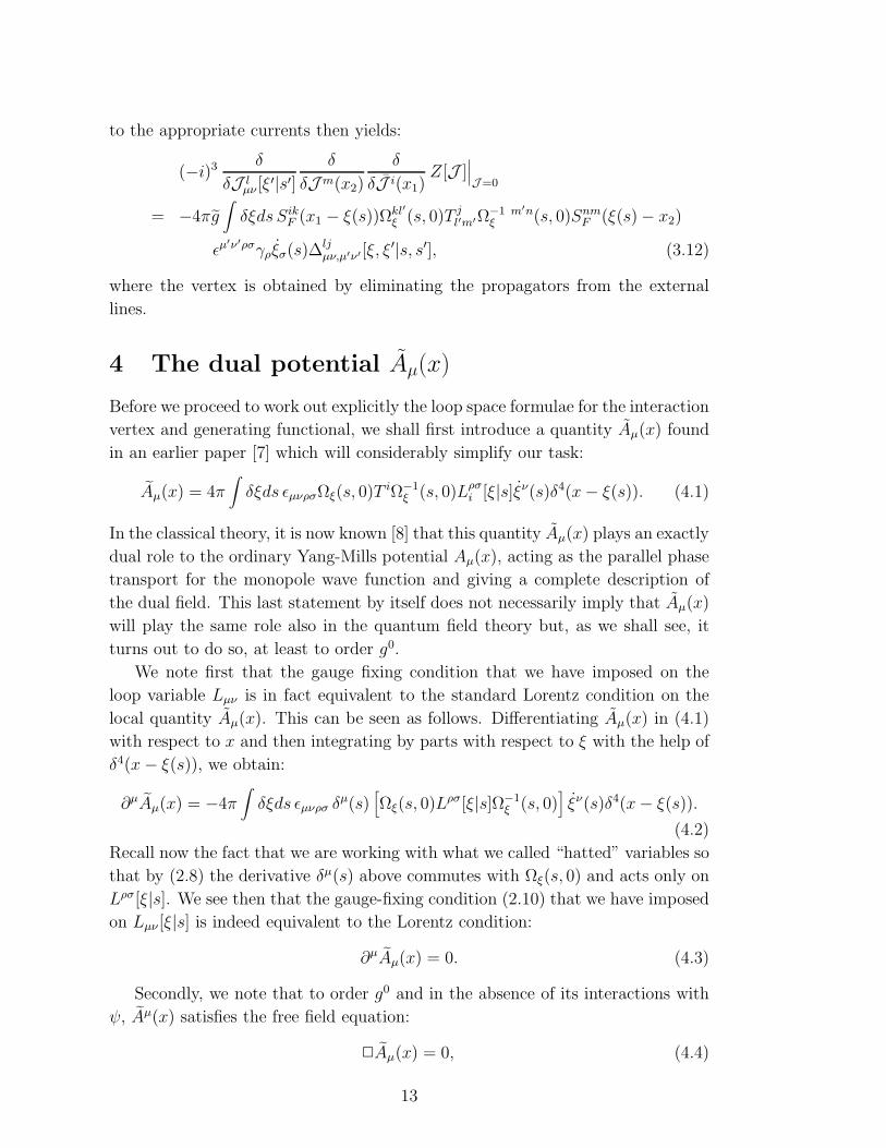
4 The dual potential Aµ(x)

Before we proceed to work out explicitly the loop space formulae for the interaction

vertex and generating functional, we shall first introduce a quantity Aµ(x) found

in an earlier paper [7] which will considerably simplify our task:

Aµ(x) = 4π∫δξds ǫµνρσΩξ(s, 0)T

iΩ−1ξ (s, 0)Lρσ

i [ξ|s]ξν(s)δ4(x− ξ(s)). (4.1)

In the classical theory, it is now known [8] that this quantity Aµ(x) plays an exactly

dual role to the ordinary Yang-Mills potential Aµ(x), acting as the parallel phase

transport for the monopole wave function and giving a complete description of

the dual field. This last statement by itself does not necessarily imply that Aµ(x)

will play the same role also in the quantum field theory but, as we shall see, it

turns out to do so, at least to order g0.

We note first that the gauge fixing condition that we have imposed on the

loop variable Lµν is in fact equivalent to the standard Lorentz condition on the

local quantity Aµ(x). This can be seen as follows. Differentiating Aµ(x) in (4.1)

with respect to x and then integrating by parts with respect to ξ with the help of

δ4(x− ξ(s)), we obtain:

∂µAµ(x) = −4π∫δξds ǫµνρσ δ

µ(s)[Ωξ(s, 0)L

ρσ[ξ|s]Ω−1ξ (s, 0)

]ξν(s)δ4(x− ξ(s)).

(4.2)

Recall now the fact that we are working with what we called “hatted” variables so

that by (2.8) the derivative δµ(s) above commutes with Ωξ(s, 0) and acts only on

Lρσ[ξ|s]. We see then that the gauge-fixing condition (2.10) that we have imposed

on Lµν [ξ|s] is indeed equivalent to the Lorentz condition:

∂µAµ(x) = 0. (4.3)

Secondly, we note that to order g0 and in the absence of its interactions with

ψ, Aµ(x) satisfies the free field equation:

Aµ(x) = 0, (4.4)

13

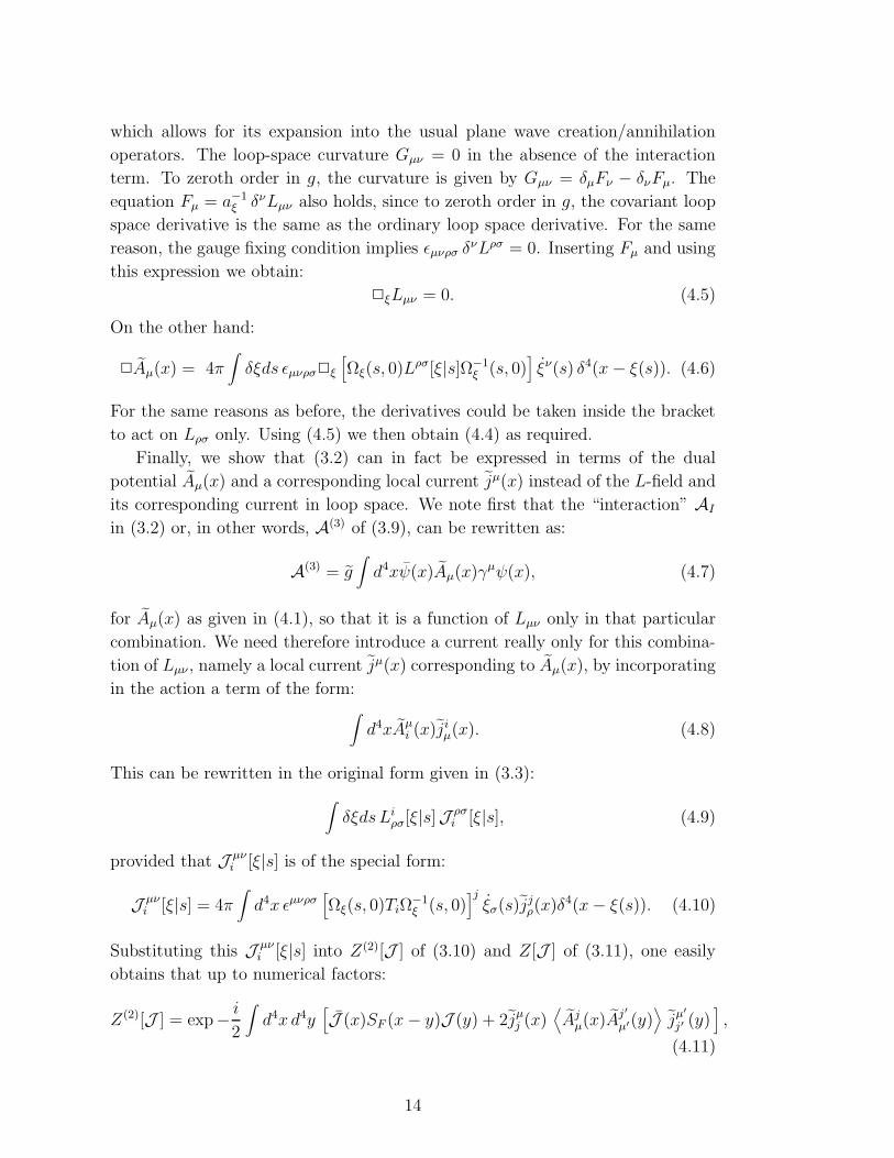
which allows for its expansion into the usual plane wave creation/annihilation

operators. The loop-space curvature Gµν = 0 in the absence of the interaction

term. To zeroth order in g, the curvature is given by Gµν = δµFν − δνFµ. The

equation Fµ = a−1ξ δνLµν also holds, since to zeroth order in g, the covariant loop

space derivative is the same as the ordinary loop space derivative. For the same

reason, the gauge fixing condition implies ǫµνρσ δνLρσ = 0. Inserting Fµ and using

this expression we obtain:

ξLµν = 0. (4.5)

On the other hand:

Aµ(x) = 4π∫δξds ǫµνρσξ

[Ωξ(s, 0)L

ρσ[ξ|s]Ω−1ξ (s, 0)

]ξν(s) δ4(x− ξ(s)). (4.6)

For the same reasons as before, the derivatives could be taken inside the bracket

to act on Lρσ only. Using (4.5) we then obtain (4.4) as required.

Finally, we show that (3.2) can in fact be expressed in terms of the dual

potential Aµ(x) and a corresponding local current jµ(x) instead of the L-field and

its corresponding current in loop space. We note first that the “interaction” AI

in (3.2) or, in other words, A(3) of (3.9), can be rewritten as:

A(3) = g∫d4xψ(x)Aµ(x)γ

µψ(x), (4.7)

for Aµ(x) as given in (4.1), so that it is a function of Lµν only in that particular

combination. We need therefore introduce a current really only for this combina-

tion of Lµν , namely a local current jµ(x) corresponding to Aµ(x), by incorporating

in the action a term of the form:∫d4xAµ

i (x)jiµ(x). (4.8)

This can be rewritten in the original form given in (3.3):

∫δξds Li

ρσ[ξ|s]Jρσi [ξ|s], (4.9)

provided that J µνi [ξ|s] is of the special form:

J µνi [ξ|s] = 4π

∫d4x ǫµνρσ

[Ωξ(s, 0)TiΩ

−1ξ (s, 0)

]jξσ(s)j

jρ(x)δ

4(x− ξ(s)). (4.10)

Substituting this J µνi [ξ|s] into Z(2)[J ] of (3.10) and Z[J ] of (3.11), one easily

obtains that up to numerical factors:

Z(2)[J ] = exp−i

2

∫d4x d4y

[J (x)SF (x− y)J (y) + 2jµj (x)

⟨Aj

µ(x)Aj′

µ′(y)⟩jµ

′

j′ (y)],

(4.11)

14

and that:

Z[J ] =

[1 + ig

∫d4x d4y d4z d4w J i(x)Sik

F (x− w)T knj

Sni′

F (w − y)J i′(y)γρ⟨Aj

ρ(x)Aj′

ρ′(z)⟩jρ

′

j′ (z)

]Z(2)[J ], (4.12)

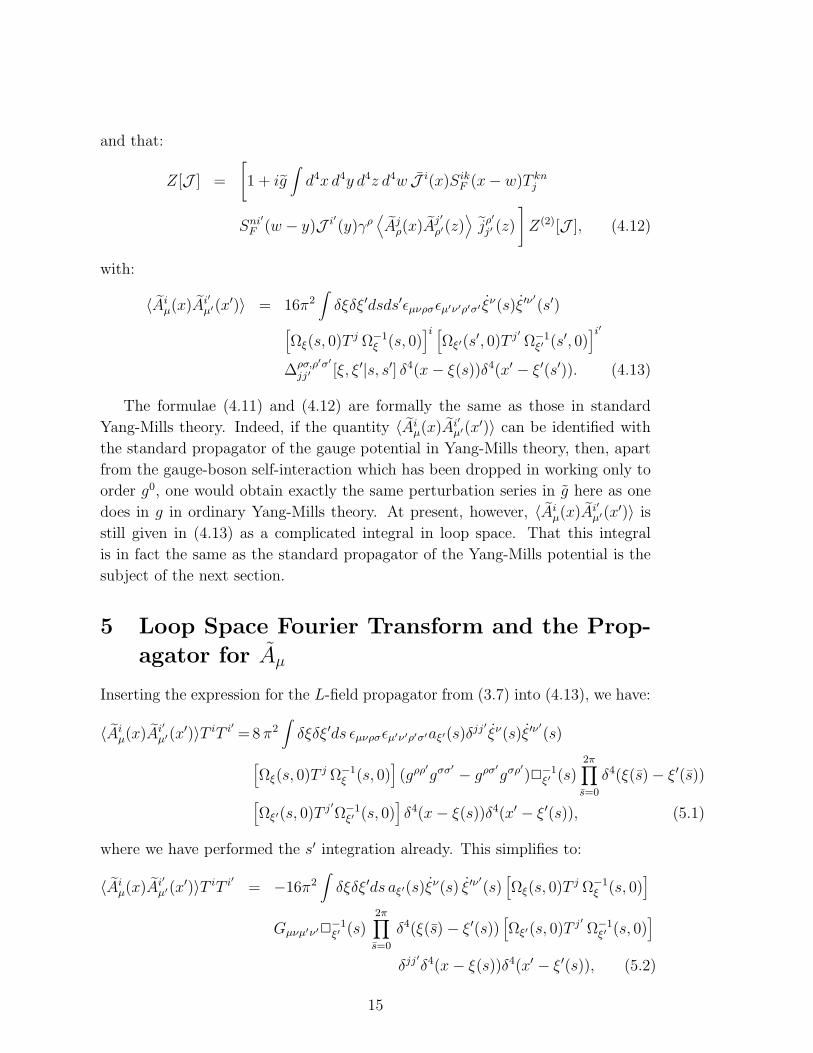
with:

〈Aiµ(x)A

i′

µ′(x′)〉 = 16π2∫δξδξ′dsds′ǫµνρσǫµ′ν′ρ′σ′ ξν(s)ξ′ν

′

(s′)

[Ωξ(s, 0)T

j Ω−1ξ (s, 0)

]i [Ωξ′(s

′, 0)T j′ Ω−1ξ′ (s

′, 0)]i′

∆ρσ,ρ′σ′

jj′ [ξ, ξ′|s, s′] δ4(x− ξ(s))δ4(x′ − ξ′(s′)). (4.13)

The formulae (4.11) and (4.12) are formally the same as those in standard

Yang-Mills theory. Indeed, if the quantity 〈Aiµ(x)A

i′

µ′(x′)〉 can be identified with

the standard propagator of the gauge potential in Yang-Mills theory, then, apart

from the gauge-boson self-interaction which has been dropped in working only to

order g0, one would obtain exactly the same perturbation series in g here as one

does in g in ordinary Yang-Mills theory. At present, however, 〈Aiµ(x)A

i′

µ′(x′)〉 is

still given in (4.13) as a complicated integral in loop space. That this integral

is in fact the same as the standard propagator of the Yang-Mills potential is the

subject of the next section.

5 Loop Space Fourier Transform and the Prop-

agator for Aµ

Inserting the expression for the L-field propagator from (3.7) into (4.13), we have:

〈Aiµ(x)A

i′

µ′(x′)〉T iT i′ =8 π2∫δξδξ′ds ǫµνρσǫµ′ν′ρ′σ′aξ′(s)δ

jj′ ξν(s)ξ′ν′

(s)

[Ωξ(s, 0)T

j Ω−1ξ (s, 0)

](gρρ

′

gσσ′

− gρσ′

gσρ′

)−1ξ′ (s)

2π∏

s=0

δ4(ξ(s)− ξ′(s))

[Ωξ′(s, 0)T

j′Ω−1ξ′ (s, 0)

]δ4(x− ξ(s))δ4(x′ − ξ′(s)), (5.1)

where we have performed the s′ integration already. This simplifies to:

〈Aiµ(x)A

i′

µ′(x′)〉T iT i′ = −16π2∫δξδξ′ds aξ′(s)ξ

ν(s) ξ′ν′

(s)[Ωξ(s, 0)T

j Ω−1ξ (s, 0)

]

Gµνµ′ν′−1ξ′ (s)

2π∏

s=0

δ4(ξ(s)− ξ′(s))[Ωξ′(s, 0)T

j′ Ω−1ξ′ (s, 0)

]

δjj′

δ4(x− ξ(s))δ4(x′ − ξ′(s)), (5.2)

15

where we have used the abbreviation:

Gµνµ′ν′ = (gµµ′gνν′ − gµν′gνµ′). (5.3)

Using the bra-ket notation of Dirac, we now define:

〈x|Γνj |ξ〉 = 4πi ξν(s)

[Ωξ(s, 0)T

j Ω−1ξ (s, 0)

]δ4(x− ξ(s)), (5.4)

〈ξ|∆jj′

µνµ′ν′ |ξ′〉 = aξ′(s)Gµνµ′ν′δ

jj′

−1ξ′ (s)

2π∏

s=0

δ4(ξ(s)− ξ′(s)), (5.5)

and write:

〈Aiµ(x)A

i′

µ′(x′)〉T iT i′ =∫ds 〈x|Ωµµ′ |x′〉, (5.6)

with:

Ωµµ′ = Γνj∆

jj′

µνµ′ν′Γν′

j′ . (5.7)

Our aim now is to transform this propagator to momentum space so as to

compare with the standard propagator of the Yang-Mills potential. Although

this propagator is itself an ordinary space-time quantity for which the Fourier

transform is well-defined, it is expressed in terms of loop quantities the Fourier

transformation of which will require some care. First, if in analogy to 〈x|p〉 =

exp (−ipx) in ordinary space-time, we define in loop space:

〈ξ|π〉 =∫dt exp i ξ(t)π(t). (5.8)

then we can write:

〈p|Γνj |π〉 = i

∫d4x δξ 〈p|x〉〈x|Γ|ξ〉〈ξ|π〉

= i∫δξ eip ξ(s) 4πξν(s)

[ΩξT

j Ω−1ξ

]exp−i

∫dt ξ(t)π(t), (5.9)

〈π′|Γ′ν′

j |p′〉 = i∫δξ′ e−ip′ξ′(s)4πξν

′

(s)[Ωξ′T

j′Ω−1ξ′

]exp i

∫dt ξ′(t)π′(t). (5.10)

and:

〈π|∆jj′

µµ′νν′|π′〉 =

∫δξ δξ′ aξ(s)

[Gµνµ′ν′δ

jj′

−1ξ′ (s)

2π∏

s=0

δ4(ξ(s)− ξ′(s))

]

(exp i

∫ 2π

0dt π(t)ξ(t)

) (exp−i

∫ 2π

0dt π′(t)ξ′(t)

). (5.11)

However, if we proceed now to evaluate these quantities, we shall find δ-functional

ambiguities connected with the definition of the loop derivative δµ(s) = δ/δξµ(s)

and the tangent to the loop ξµ(s) both of which occur in the formulae above.

In other words, some regularization procedure is required in order to give these

quantities an unambiguous meaning. Our procedure, which we have followed

16

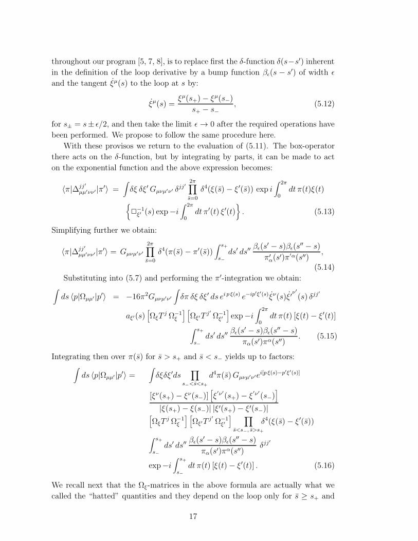
throughout our program [5, 7, 8], is to replace first the δ-function δ(s−s′) inherent

in the definition of the loop derivative by a bump function βǫ(s − s′) of width ǫ

and the tangent ξµ(s) to the loop at s by:

ξµ(s) =ξµ(s+)− ξµ(s−)

s+ − s−, (5.12)

for s± = s± ǫ/2, and then take the limit ǫ→ 0 after the required operations have

been performed. We propose to follow the same procedure here.

With these provisos we return to the evaluation of (5.11). The box-operator

there acts on the δ-function, but by integrating by parts, it can be made to act

on the exponential function and the above expression becomes:

〈π|∆jj′

µµ′νν′|π′〉 =

∫δξ δξ′Gµνµ′ν′ δ

jj′2π∏

s=0

δ4(ξ(s)− ξ′(s)) exp i∫ 2π

0dt π(t)ξ(t)

−1ξ′ (s) exp−i

∫ 2π

0dt π′(t) ξ′(t)

. (5.13)

Simplifying further we obtain:

〈π|∆jj′

µµ′νν′|π′〉 = Gµνµ′ν′

2π∏

s=0

δ4(π(s)− π′(s))∫ s+

s−

ds′ ds′′βǫ(s

′ − s)βǫ(s′′ − s)

π′α(s

′)π′α(s′′),

(5.14)

Substituting into (5.7) and performing the π′-integration we obtain:∫ds 〈p|Ωµµ′ |p′〉 = −16π2Gµνµ′ν′

∫δπ δξ δξ′ ds ei p ξ(s) e−ip′ξ′(s)ξν(s)ξ′

ν′

(s) δjj′

aξ′(s)[ΩξT

j Ω−1ξ

] [Ωξ′T

j′ Ω−1ξ′

]exp−i

∫ 2π

0dt π(t) [ξ(t)− ξ′(t)]

∫ s+

s−

ds′ ds′′βǫ(s

′ − s)βǫ(s′′ − s)

πα(s′)πα(s′′). (5.15)

Integrating then over π(s) for s > s+ and s < s− yields up to factors:∫ds 〈p|Ωµµ′|p′〉 =

∫δξδξ′ds

∏

s−<s<s+

d4π(s)Gµνµ′ν′ei[p ξ(s)−p′ξ′(s)]

[ξν(s+)− ξν(s−)][ξ′ν′(s+)− ξ

′ν′(s−)]

|ξ(s+)− ξ(s−)| |ξ′(s+)− ξ′(s−)|[ΩξT

j Ω−1ξ

] [Ωξ′T

j′ Ω−1ξ′

] ∏

s<s−, s>s+

δ4(ξ(s)− ξ′(s))

∫ s+

s−

ds′ ds′′βǫ(s

′ − s)βǫ(s′′ − s)

πα(s′)πα(s′′)δjj

′

exp−i∫ s+

s−

dt π(t) [ξ(t)− ξ′(t)] . (5.16)

We recall next that the Ωξ-matrices in the above formula are actually what we

called the “hatted” quantities and they depend on the loop only for s ≥ s+ and

17

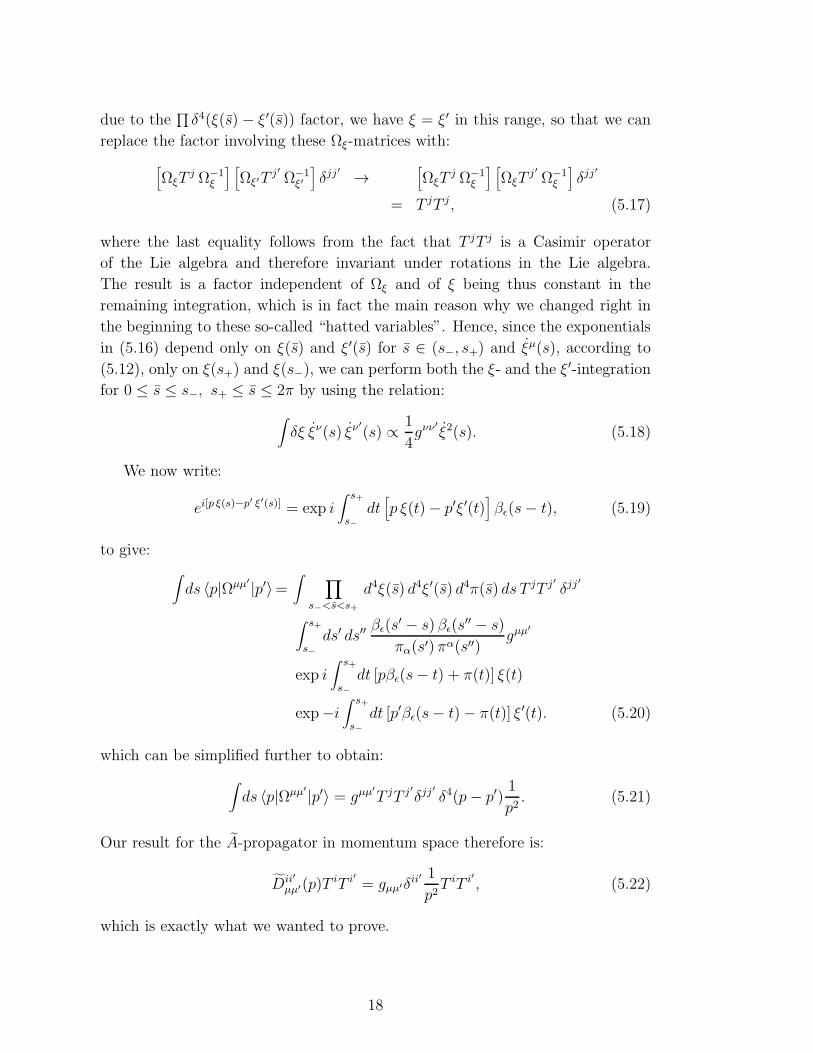
due to the∏δ4(ξ(s)− ξ′(s)) factor, we have ξ = ξ′ in this range, so that we can

replace the factor involving these Ωξ-matrices with:

[ΩξT

j Ω−1ξ

] [Ωξ′T

j′ Ω−1ξ′

]δjj

′

→[ΩξT

j Ω−1ξ

] [ΩξT

j′ Ω−1ξ

]δjj

′

= T jT j, (5.17)

where the last equality follows from the fact that T jT j is a Casimir operator

of the Lie algebra and therefore invariant under rotations in the Lie algebra.

The result is a factor independent of Ωξ and of ξ being thus constant in the

remaining integration, which is in fact the main reason why we changed right in

the beginning to these so-called “hatted variables”. Hence, since the exponentials

in (5.16) depend only on ξ(s) and ξ′(s) for s ∈ (s−, s+) and ξµ(s), according to

(5.12), only on ξ(s+) and ξ(s−), we can perform both the ξ- and the ξ′-integration

for 0 ≤ s ≤ s−, s+ ≤ s ≤ 2π by using the relation:

∫δξ ξν(s) ξν

′

(s) ∝1

4gνν

′

ξ2(s). (5.18)

We now write:

ei[p ξ(s)−p′ ξ′(s)] = exp i∫ s+

s−

dt[p ξ(t)− p′ξ′(t)

]βǫ(s− t), (5.19)

to give:

∫ds 〈p|Ωµµ′

|p′〉=∫ ∏

s−<s<s+

d4ξ(s) d4ξ′(s) d4π(s) ds T jT j′ δjj′

∫ s+

s−

ds′ ds′′βǫ(s

′ − s) βǫ(s′′ − s)

πα(s′) πα(s′′)gµµ

′

exp i∫ s+

s−

dt [pβǫ(s− t) + π(t)] ξ(t)

exp−i∫ s+

s−

dt [p′βǫ(s− t)− π(t)] ξ′(t). (5.20)

which can be simplified further to obtain:

∫ds 〈p|Ωµµ′

|p′〉 = gµµ′

T jT j′δjj′

δ4(p− p′)1

p2. (5.21)

Our result for the A-propagator in momentum space therefore is:

Dii′

µµ′(p)T iT i′ = gµµ′δii′ 1

p2T iT i′, (5.22)

which is exactly what we wanted to prove.

18

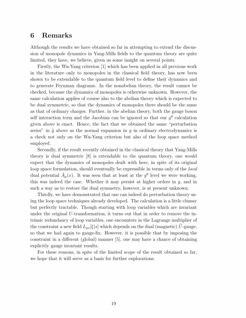
6 Remarks

Although the results we have obtained so far in attempting to extend the discus-

sion of monopole dynamics in Yang-Mills fields to the quantum theory are quite

limited, they have, we believe, given us some insight on several points.

Firstly, the Wu-Yang criterion [1] which has been applied in all previous work

in the literature only to monopoles in the classical field theory, has now been

shown to be extendable to the quantum field level to define their dynamics and

to generate Feynman diagrams. In the nonabelian theory, the result cannot be

checked, because the dynamics of monopoles is otherwise unknown. However, the

same calculation applies of course also to the abelian theory which is expected to

be dual symmetric, so that the dynamics of monopoles there should be the same

as that of ordinary charges. Further, in the abelian theory, both the gauge boson

self interaction term and the Jacobian can be ignored so that our g0 calculation

given above is exact. Hence, the fact that we obtained the same “perturbation

series” in g above as the normal expansion in g in ordinary electrodynamics is

a check not only on the Wu-Yang criterion but also of the loop space method

employed.

Secondly, if the result recently obtained in the classical theory that Yang-Mills

theory is dual symmetric [8] is extendable to the quantum theory, one would

expect that the dynamics of monopoles dealt with here, in spite of its original

loop space formulation, should eventually be expressible in terms only of the local

dual potential Aµ(x). It was seen that at least at the g0 level we were working,

this was indeed the case. Whether it may persist at higher orders in g, and in

such a way as to restore the dual symmetry, however, is at present unknown.

Thirdly, we have demonstrated that one can indeed do perturbation theory us-

ing the loop space techniques already developed. The calculation is a little clumsy

but perfectly tractable. Though starting with loop variables which are invariant

under the original U -transformation, it turns out that in order to remove the in-

trinsic redundancy of loop variables, one encounters in the Lagrange multiplier of

the constraint a new field Lµν [ξ|s] which depends on the dual (magnetic) U -gauge,

so that we had again to gauge-fix. However, it is possible that by imposing the

constraint in a different (global) manner [5], one may have a chance of obtaining

explicitly gauge invariant results.

For these reasons, in spite of the limited scope of the result obtained so far,

we hope that it will serve as a basis for further explorations.

19

7 Acknowledgements

JF acknowledges the support of the Mihran and Azniv Essefian Foundation (Lon-

don), the Soudavar Foundation (Oxford) and the Calouste Gulbenkian Foundation

(Lisbon), JP is grateful to Studienstiftung d.d. Volkes for financial support and

TST thanks the Wingate Foundation for partial support during most of this work.

References

[1] T.T. Wu and C.N. Yang, Phys. Rev. D14. 437 (1976).

[2] E. Lubkin, Ann. Phys. N.Y. 23 233 (1963).

[3] T.S. Wu and C.N. Yang, Phys. Rev. D12 (1975) 3845.

[4] S. Coleman (1974), in Proceedings of the 1974 Erice School (Plenum, New

York, 1975), p. 297.

[5] Chan Hong-Mo, P. Scharbach and Tsou Sheung Tsun, Ann. Phys. (N.Y.)

167 454 (1986); ibid. 166 396 (1986); Chan Hong-Mo and Tsou Sheung

Tsun, Act. Phys. Pol. B17, 259 (1986).

[6] Chan Hong-Mo and Tsou Sheung Tsun, Some Elementary Gauge Theory

Concepts (World Scientific, London-New York-Singapore, 1993).

[7] Chan Hong-Mo, J. Faridani and Tsou Shueng Tsun, Phys. Rev. D51 7040

(1995); ibid. D52 6134 (1995).

[8] Chan Hong-Mo, J. Faridani and Tsou Sheung Tsun, Rutherford Appleton

Laboratory preprint, RAL-TR-95-076 (1995), hep-th 9512173, to appear in

Phys. Rev. D.

[9] N. Seiberg and E. Witten, Nucl. Phys. B426, 19 (1994); B431, 484 (1994).

[10] K. Intriligator and N. Seiberg, Nucl. Phys. B431, 551 (1994); N. Seiberg,

ibid. B435, 129 (1995); N. Seiberg, in Particles, Strings, and Cosmology,

Proceedings of the Workshop, Syracuse, New York, 1994, edited by K.C.

Wali (World Scientific, Singapore, 1995).

[11] C. Vafa and E. Witten, Nucl. Phys. B431, 3 (1994); E. Witten, Math. Res.

Lett. 1, 769 (1994).

[12] O. Aharony, Phys. Lett. 351B, 220 (1995); L. Girardello, A. Giveon, M.

Porrati, and A. Zaffaroni, Nucl. Phys. B448, 127 (1995), hep-th/9507064; A.

Ceresole, R. D’Auria, S. Ferrara and A. Van Proeyen, Nucl. Phys. B444 92

20

(1995); J.A. Harvey, G. Moore and A. Strominger, hep-th/9501022; R.G.

Leigh and M.J. Strassler, Nucl. Phys. B447, 95 (1995); E. Comay hep-

th/9503234; D. Kutasov and A. Schwimmer, Phys. Lett. 354B, 315 (1995);

K. Intriligator and P. Pouliot, Phys. Lett. 353B, 471 (1995); K. Intriligator,

Nucl. Phys. B448, 187 (1995); C. Gomez and E. Lopez, Phys. Lett. 357B,

558 (1995); E. Witten, hep-th/9505186; G.W. Gibbons and D.A. Rasheed,

Nucl. Phys. B454, 185 (1995); K. Intriligator, R.G. Leigh and M.J. Strassler,

Nucl. Phys. B456, 567 (1995); N. Mohammedi, hep-th/9507040; E. Alvarez,

L. Alvarez-Gaume and I. Bakas, Nucl. Phys. B457, 3 (1995); Y. Lozano,

Phys. Lett. B364, 19 (1995); D. Olive, hep-th/9508091; C. Ford and I.

Sachs, Phys. Lett. B362, 88 (1995); O. Aharony and S. Yankielowicz, hep-

th/9601011; Kimyeong Lee, E.J. Weinberg and Piljin Yi, hep-th/9601097;

S.F. Hewson and M.J. Perry, hep-th/9603015. The above is still only a par-

tial list of the many articles which have recently appeared on the subject.

[13] A.M. Polyakov, Nucl. Phys. B164, 171 (1980)

[14] J. Faridani, D. Phil. thesis: University of Oxford, 1994.

[15] Jakov Pfaudler, M.Sc. thesis: University of Oxford, 1995.

[16] Particle Physics Booklet (ed. M. Aguilar-Benitez et al., American Institute

of Physics, 1994) p. 202.

[17] D. Freedman and P.K. Townsend, Nucl. Phys. B177, 282 (1981).

[18] M.A. Namazie and D. Storey, Nucl. Phys. B157, 170 (1979).

[19] W. Siegel, Phys. Lett. 93B, 170 (1980).

[20] G.L. Demarco, C. Fosco and R.C. Trinchero, Phys. Rev. D45, 3701 (1992).

21