Running head: CUDA-BASED GLOBAL ILLUMINATION 1 · Running head: CUDA-BASED GLOBAL ILLUMINATION 1 CUDA-Based Global Illumination Aaron Jensen San Jose State University 13 May, 2014

Running head: CUDA-BASED GLOBAL ILLUMINATION 1

CUDA-Based Global Illumination

Aaron Jensen

San Jose State University

13 May, 2014

CS 180H: Independent Research for Department Honors

Author Note

Aaron Jensen, Undergraduate, Department of Computer Science, San Jose State University.

Research was conducted under the guidance of Dr. Pollett, Department of Computer Science,

San Jose State University.

CUDA-BASED GLOBAL ILLUMINATION 2

Abstract

This paper summarizes a semester of individual research on NVIDIA CUDA programming and

global illumination. What started out as an attempt to update a CPU-based radiosity engine from

a previous graphics class evolved into an exploration of other lighting techniques and models

(collectively known as global illumination) and other graphics-based languages (OpenCL and

GLSL). After several attempts and roadblocks, the final software project is a CUDA-based port

of David Bucciarelli's SmallPt GPU, which itself is an OpenCL-based port of Kevin Beason's

smallpt. The paper concludes with potential additions and alterations to the project.


CUDA-Based Global Illumination

Accurately representing lighting in computer graphics has been a topic that spans many

fields and applications: mock-ups for architecture, environments in video games and computer

generated images in movies to name a few (Dutré). One of the biggest issues with performing

lighting calculations is that they typically take an enormous amount of time and resources to

calculate accurately (Teoh). There have been many advances in lighting algorithms to reduce the

time spent in calculations. One common approach is to approximate a solution rather than

perform an exhaustive calculation of a true solution. The evolution of multi-core graphics cards

has also proved very interesting. What once was computed on a single or dual-core CPU can

now be offloaded to several-hundred to several-thousand-core GPUs. While each individual

GPU core may not be as fast as a single CPU core, parallelization of work can greatly reduce

time needed to compute for properly designed algorithms (Luebke).

The purpose of this project is to gain experience with CUDA as a general purpose

computing platform via a global illumination engine.

Background

What is Global Illumination?

First we break down the term "global illumination." Because the final visualization of an

object in a scene is dependent on the light that hits it from the whole environment, we say it is

"global." "Illumination" is used because we are strictly discussing how light interacts with these

objects in a scene (Dutré). It is important to note that there are two main approaches to

approximating true global illumination: radiosity and ray tracing. Ray tracing is preferred for

specular highlights because individual rays are traced from the eye through each pixel in a frame


and are reflected about a scene to compute a final color. Unfortunately, we do not live in glass

houses made of perfectly shiny materials. Traditional ray tracing largely ignores diffuse

reflections. This is where radiosity comes into play: radiosity deals with the diffuse reflections

and bleeding of colors amongst objects by simulating light bouncing off objects. However,

radiosity largely ignores specular reflections (Teoh). As we will see in the final project, we can

blend both ray tracing and radiosity to create very realistic computer generated images.

The Cornell Box

The Cornell Box originated from the Cornell University Program of Computer Graphics

in 1984. It was featured in a SIGGRAPH paper Modeling the Interaction of Light Between

Diffuse Surfaces. The basic structure is described as a cubic room with a red wall on the left and

a green or blue wall on the right. The ceiling, floor and back wall are typically white. There is a

single light in the center of the ceiling to illuminate the room. Although the original Cornell Box

was a room without any objects, it has been infinitely modified and is widely considered the

standard for multiple graphics simulations. Cubes, spheres, water, dragons and bunnies made

from a variety of diffuse, reflective and refractive materials, can be found neatly housed in a

Cornell Box simply by searching Google Images for "Cornell Box" (Teoh).

Why CUDA?

From the start, I was biased because I have always purchased NVIDIA graphics cards for

my personal computers and had recently purchased a Razer Blade laptop with a GeForce 765M

NVIDIA card. The two leaders for general purpose GPU computing at the time I was doing

preliminary research (summer of 2013) were OpenCL (widely supported on ATI and NVIDIA

graphics cards) and CUDA (NVIDIA only). Unfortunately, the online documentation for

OpenCL was a mess at this time; there were broken links and conflicting information on


different webpage's. CUDA, however, had a very nice developer's webpage and there were

several modern books and resources available. For these reasons, I choose to pursue CUDA as

the primary language for this project.

Monte Carlo Sampling

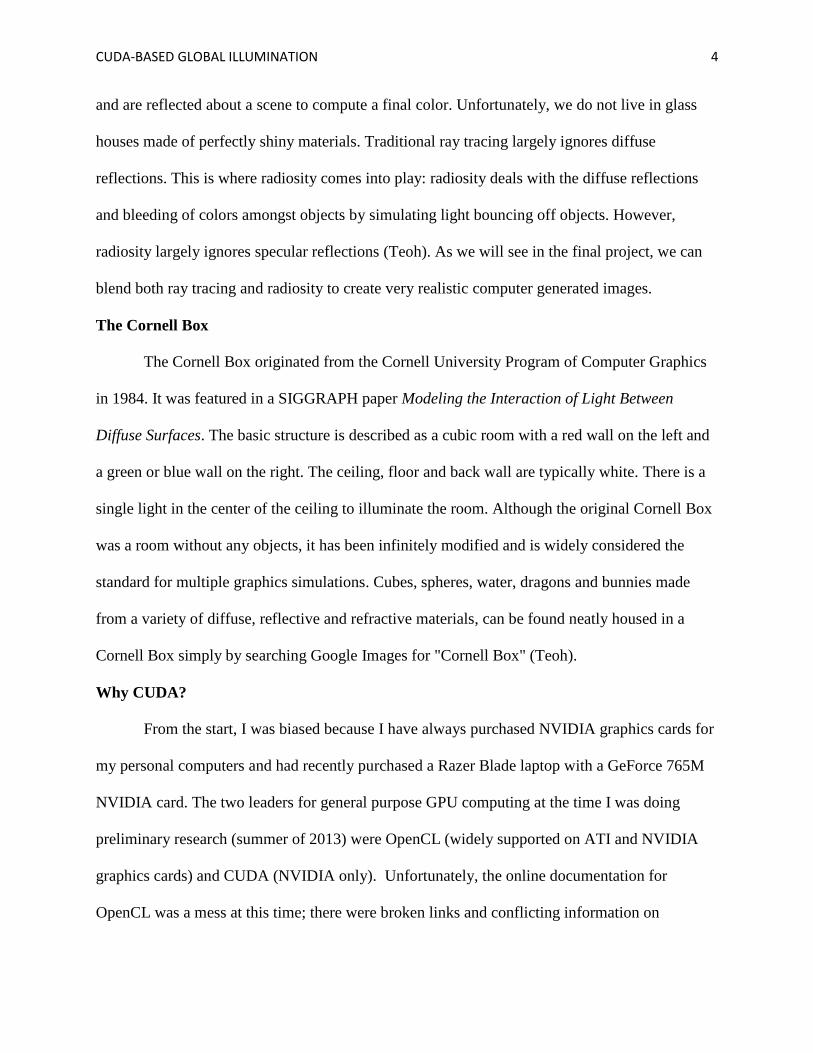
One of the important techniques used in the global illumination technique used in the

final project is Monte Carlo sampling. In this application, when a ray intersects an object, it is

bounced off at a random angle. By taking an average of multiple random samples, we converge

on the solution. Although this idea is easy to explain, in practice it converges at a rate of

for N

samples (Dutré). This is one potential cause for the graininess that is visible in the final images

of the original smallpt algorithm seen below in Figure 1:

Figure 1. Graininess of smallpt generated images. This figure depicts a drawback to Monte Carlo

methods.

It is appropriate to point out some of the run times of the CPU variant of smallpt here. A

reasonable sample takes about five minutes to compute using four CPU threads (approximately

200 samples) (Beason). To put this in perspective, last year when I took CS 116B I created a


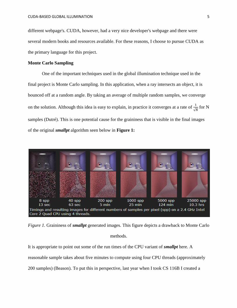
CPU-based radiosity engine which followed the traditional radiosity approach. It took five

minutes to create the image in Figure 2.

Figure 2. Traditional CPU-based Radiosity. Image took five minutes to generate.

Traditional Radiosity

Traditional radiosity involves computing the color for each patch of each surface by

summing the light that it "sees." As can be seen in Figure 2, each surface is subdivided into

many smaller patches. One can move the camera from each patch and sample the light that hits it

from every other patch (the gathering phase). This is typically implemented by rendering each

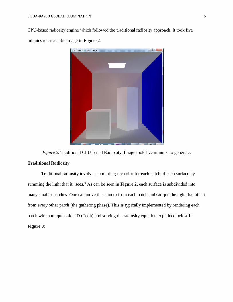
patch with a unique color ID (Teoh) and solving the radiosity equation explained below in

Figure 3:


Figure 3. The Radiosity Equation. How to calculate the color of a patch (Spencer).

Starting by emitting light only from light sources and then letting the light "bounce" around the

scene, actual lighting can be approximated given enough iterations. As one could imagine,

rendering the scene from every patch can be very costly with respect to time.

Development

Initial Approach and Evolution

My initial approach was to calculate all of the patch colors in CUDA. This proved to be

more troublesome than initially anticipated. One of the improvements I was trying to implement

to optimize for time was the idea of adaptive subdivision. Rather than subdividing each surface

into a fixed grid of patches, I would start with a rather low resolution quad tree for each surface

and subdivide as needed when patches differed too much (e.g. corners and sharp shadows)

(Coombe). Learning CUDA and implementing an unfamiliar algorithm proved more time

consuming than anticipated; I moved on to evolving my approach.


I began working on the Udacity course for parallel programming to introduce me to

CUDA. One of the most frustrating things was that CUDA code was not running on my

computer despite having a NVIDIA graphics card. I finally figured out that NVIDIA Optimus

technology automatically switches between integrated and dedicated graphics to optimize battery

life. Once I forced Visual Studio to use the dedicated card, CUDA samples and programming

worked (Luebke). While I was conducting the research for this paper, I was concurrently

employed as a grader for CS 116B being taught by Dr. Pollett. When I took CS 116B a year ago

under Dr. Teoh, the course focused on OpenGL 1.x and 2.x. Dr. Pollett's 116B focused on using

modern OpenGL in tandem with GLSL. This provided new insights and approaches to solving

the problems that had arisen. I spent some time learning basic GLSL for grading as well as

attempting to implement a radiosity fragment and vertex shader from scratch (Gortler). This also

proved to be a very time consuming task and very difficult to balance with my final semester.

With deadlines quickly approaching, it was time to focus back on CUDA.

I found a wonderful project named smallpt by Beason. As its name implies, it is global

illumination in 99 lines of C++ code. What was most beneficial was that Bucciarelli had spent

the time implementing it in OpenCL. After discussing with Dr. Pollett, I switched gears to

implementing a port of SmallPt GPU to CUDA. This closely followed my original intent of

learning CUDA by implementing a global illumination engine. This would also serve as a nice

opportunity to compare OpenCL and CUDA.


Final Implementation

Porting to CUDA

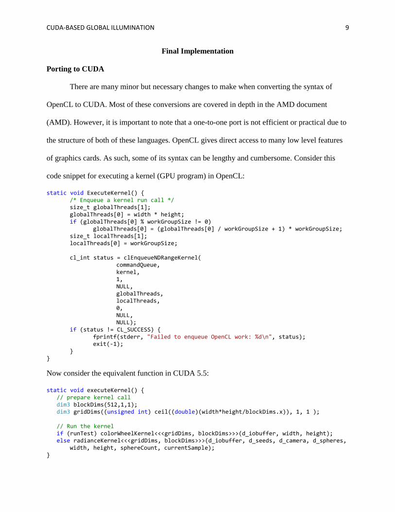
There are many minor but necessary changes to make when converting the syntax of

OpenCL to CUDA. Most of these conversions are covered in depth in the AMD document

(AMD). However, it is important to note that a one-to-one port is not efficient or practical due to

the structure of both of these languages. OpenCL gives direct access to many low level features

of graphics cards. As such, some of its syntax can be lengthy and cumbersome. Consider this

code snippet for executing a kernel (GPU program) in OpenCL:

static void ExecuteKernel() { /* Enqueue a kernel run call */ size_t globalThreads[1]; globalThreads[0] = width * height; if (globalThreads[0] % workGroupSize != 0) globalThreads[0] = (globalThreads[0] / workGroupSize + 1) * workGroupSize; size_t localThreads[1]; localThreads[0] = workGroupSize; cl_int status = clEnqueueNDRangeKernel( commandQueue, kernel, 1, NULL, globalThreads, localThreads, 0, NULL, NULL); if (status != CL_SUCCESS) { fprintf(stderr, "Failed to enqueue OpenCL work: %d\n", status); exit(-1); } }

Now consider the equivalent function in CUDA 5.5:

static void executeKernel() { // prepare kernel call dim3 blockDims(512,1,1); dim3 gridDims((unsigned int) ceil((double)(width*height/blockDims.x)), 1, 1 ); // Run the kernel if (runTest) colorWheelKernel<<<gridDims, blockDims>>>(d_iobuffer, width, height); else radianceKernel<<<gridDims, blockDims>>>(d_iobuffer, d_seeds, d_camera, d_spheres, width, height, sphereCount, currentSample); }


Almost immediately, one notices that CUDA 5.5 syntax is much more succinct than OpenCL.

Whereas OpenCL sets up and manages queues to process commands, a CUDA kernel is simply

called via syntax very similar to a function call in C/C++. The only difference is some extra

parameters in <<<gridDims, blockDims >>>, which help define the structure of how the CUDA

cores should process the data. Overall, I was able to reduce ~1450 lines of code in OpenCL over

three files (geomfunc.h, smallptGPU.c, and rendering_kernel.cl) to ~750 lines of code while

adding extensive comments in one file (SmallPtCUDA.cu). This is roughly a source code

reduction of about half to write in CUDA 5.5 when compared to OpenCL.

CUDA Memory Structure

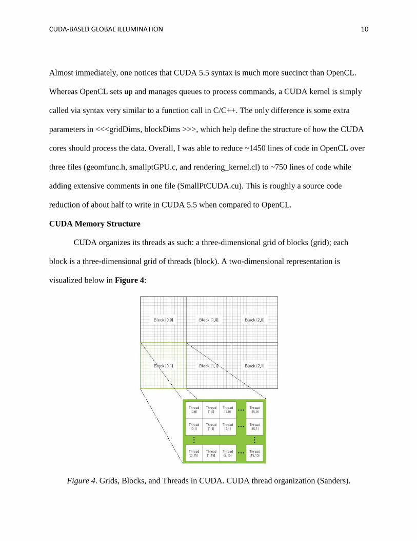
CUDA organizes its threads as such: a three-dimensional grid of blocks (grid); each

block is a three-dimensional grid of threads (block). A two-dimensional representation is

visualized below in Figure 4:

Figure 4. Grids, Blocks, and Threads in CUDA. CUDA thread organization (Sanders).


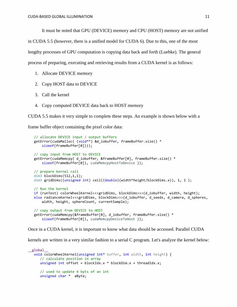
It must be noted that GPU (DEVICE) memory and CPU (HOST) memory are not unified

in CUDA 5.5 (however, there is a unified model for CUDA 6). Due to this, one of the most

lengthy processes of GPU computation is copying data back and forth (Luebke). The general

process of preparing, executing and retrieving results from a CUDA kernel is as follows:

1. Allocate DEVICE memory

2. Copy HOST data to DEVICE

3. Call the kernel

4. Copy computed DEVICE data back to HOST memory

CUDA 5.5 makes it very simple to complete these steps. An example is shown below with a

frame buffer object containing the pixel color data:

// allocate DEVICE input / output buffers getError(cudaMalloc( (void**) &d_iobuffer, frameBuffer.size() * sizeof(frameBuffer[0]))); // copy input from HOST to DEVICE getError(cudaMemcpy( d_iobuffer, &frameBuffer[0], frameBuffer.size() * sizeof(frameBuffer[0]), cudaMemcpyHostToDevice )); // prepare kernel call dim3 blockDims(512,1,1); dim3 gridDims((unsigned int) ceil((double)(width*height/blockDims.x)), 1, 1 ); // Run the kernel if (runTest) colorWheelKernel<<<gridDims, blockDims>>>(d_iobuffer, width, height); else radianceKernel<<<gridDims, blockDims>>>(d_iobuffer, d_seeds, d_camera, d_spheres, width, height, sphereCount, currentSample); // copy output from DEVICE to HOST getError(cudaMemcpy(&frameBuffer[0], d_iobuffer, frameBuffer.size() * sizeof(frameBuffer[0]), cudaMemcpyDeviceToHost ));

Once in a CUDA kernel, it is important to know what data should be accessed. Parallel CUDA

kernels are written in a very similar fashion to a serial C program. Let's analyze the kernel below:

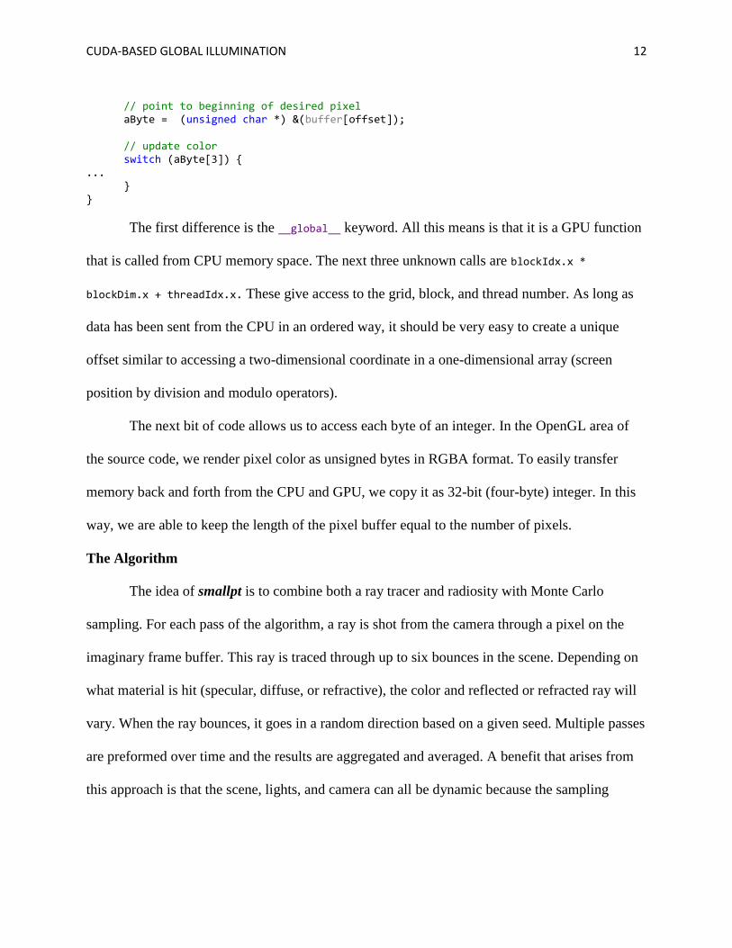
__global__ void colorWheelKernel(unsigned int* buffer, int width, int height) { // calculate position in array unsigned int offset = blockIdx.x * blockDim.x + threadIdx.x; // used to update 4 byts of an int unsigned char * aByte;


// point to beginning of desired pixel aByte = (unsigned char *) &(buffer[offset]); // update color switch (aByte[3]) { ... } }

The first difference is the __global__ keyword. All this means is that it is a GPU function

that is called from CPU memory space. The next three unknown calls are blockIdx.x *

blockDim.x + threadIdx.x. These give access to the grid, block, and thread number. As long as

data has been sent from the CPU in an ordered way, it should be very easy to create a unique

offset similar to accessing a two-dimensional coordinate in a one-dimensional array (screen

position by division and modulo operators).

The next bit of code allows us to access each byte of an integer. In the OpenGL area of

the source code, we render pixel color as unsigned bytes in RGBA format. To easily transfer

memory back and forth from the CPU and GPU, we copy it as 32-bit (four-byte) integer. In this

way, we are able to keep the length of the pixel buffer equal to the number of pixels.

The Algorithm

The idea of smallpt is to combine both a ray tracer and radiosity with Monte Carlo

sampling. For each pass of the algorithm, a ray is shot from the camera through a pixel on the

imaginary frame buffer. This ray is traced through up to six bounces in the scene. Depending on

what material is hit (specular, diffuse, or refractive), the color and reflected or refracted ray will

vary. When the ray bounces, it goes in a random direction based on a given seed. Multiple passes

are preformed over time and the results are aggregated and averaged. A benefit that arises from

this approach is that the scene, lights, and camera can all be dynamic because the sampling


process will simply reset itself. Once objects in the scene are at rest, the rendering process

continues to sample and improve the final image.

Scenes

Scenes are defined in smallpt as a series of spheres (Beason). Each sphere is described

with a radius, position, emission, color and material. The default modified Cornell Box test

image is described below:

#define WALL_RAD 1e4f static Sphere CornellSpheres[] = { /* Scene: radius, position, emission, color, material */ { WALL_RAD, {WALL_RAD + 1.f, 40.8f, 81.6f}, {0.f, 0.f, 0.f}, {.75f, .25f, .25f}, DIFF }, /*Left*/ { WALL_RAD, {-WALL_RAD + 99.f, 40.8f, 81.6f}, {0.f, 0.f, 0.f}, {.25f, .25f, .75f}, DIFF },/*Rght*/ { WALL_RAD, {50.f, 40.8f, WALL_RAD}, {0.f, 0.f, 0.f}, {.75f, .75f, .75f}, DIFF }, /* Back */ { WALL_RAD, {50.f, 40.8f, -WALL_RAD + 270.f}, {0.f, 0.f, 0.f}, {.75f, .75f, 0.f}, DIFF }, /*Frnt*/ { WALL_RAD, {50.f, WALL_RAD, 81.6f}, {0.f, 0.f, 0.f}, {.25f, .75f, .25f}, DIFF }, /* Botm */ { WALL_RAD, {50.f, -WALL_RAD + 81.6f, 81.6f}, {0.f, 0.f, 0.f}, {.75f, .75f, .75f}, DIFF }, /*Top*/ { 16.5f, {27.f, 16.5f, 47.f}, {0.f, 0.f, 0.f}, {.9f, .9f, .9f}, SPEC }, /* Mirr */ { 16.5f, {73.f, 16.5f, 78.f}, {0.f, 0.f, 0.f}, {.9f, .9f, .9f}, REFR }, /* Glas */ { 5.f, {50.f, 81.6f - 15.f, 81.6f}, {30.f, 30.f, 30.f}, {0.f, 0.f, 0.f}, DIFF } /* Light */ };

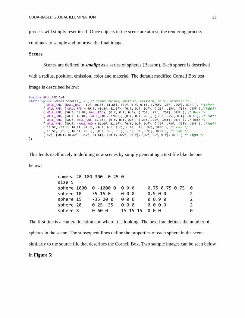
This lends itself nicely to defining new scenes by simply generating a text file like the one

below:

camera 20 100 300 0 25 0 size 5 sphere 1000 0 -1000 0 0 0 0 0.75 0.75 0.75 0 sphere 10 35 15 0 0 0 0 0.9 0 0 2 sphere 15 -35 20 0 0 0 0 0 0.9 0 2 sphere 20 0 25 -35 0 0 0 0 0 0.9 2 sphere 8 0 60 0 15 15 15 0 0 0 0

The first line is a camera location and where it is looking. The next line defines the number of

spheres in the scene. The subsequent lines define the properties of each sphere in the scene

similarly to the source file that describes the Cornell Box. Two sample images can be seen below

in Figure 5:


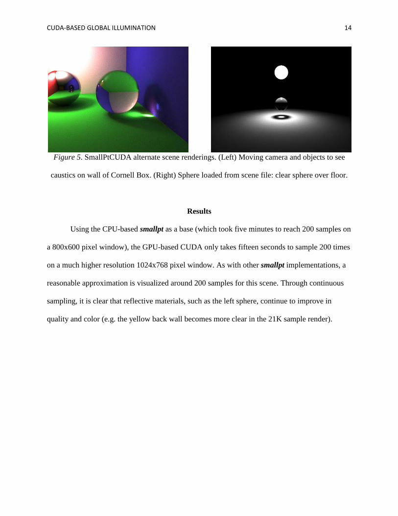
Figure 5. SmallPtCUDA alternate scene renderings. (Left) Moving camera and objects to see

caustics on wall of Cornell Box. (Right) Sphere loaded from scene file: clear sphere over floor.

Results

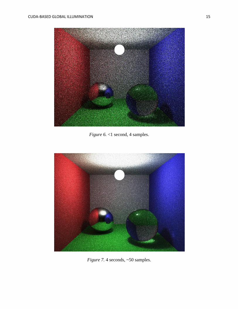
Using the CPU-based smallpt as a base (which took five minutes to reach 200 samples on

a 800x600 pixel window), the GPU-based CUDA only takes fifteen seconds to sample 200 times

on a much higher resolution 1024x768 pixel window. As with other smallpt implementations, a

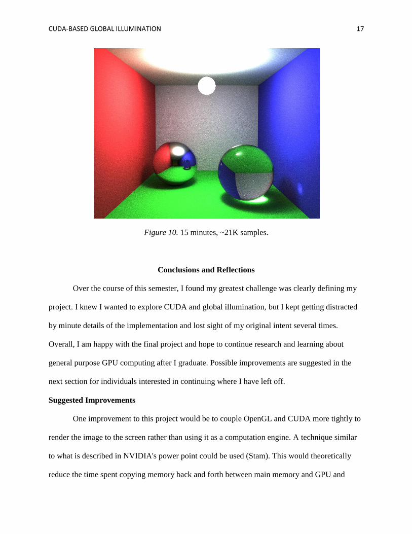
reasonable approximation is visualized around 200 samples for this scene. Through continuous

sampling, it is clear that reflective materials, such as the left sphere, continue to improve in

quality and color (e.g. the yellow back wall becomes more clear in the 21K sample render).


Figure 6. <1 second, 4 samples.

Figure 7. 4 seconds, ~50 samples.


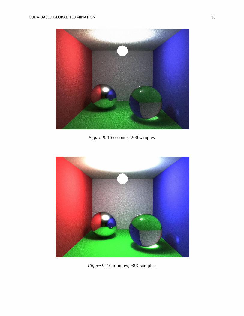
Figure 8. 15 seconds, 200 samples.

Figure 9. 10 minutes, ~8K samples.


Figure 10. 15 minutes, ~21K samples.

Conclusions and Reflections

Over the course of this semester, I found my greatest challenge was clearly defining my

project. I knew I wanted to explore CUDA and global illumination, but I kept getting distracted

by minute details of the implementation and lost sight of my original intent several times.

Overall, I am happy with the final project and hope to continue research and learning about

general purpose GPU computing after I graduate. Possible improvements are suggested in the

next section for individuals interested in continuing where I have left off.

Suggested Improvements

One improvement to this project would be to couple OpenGL and CUDA more tightly to

render the image to the screen rather than using it as a computation engine. A technique similar

to what is described in NVIDIA's power point could be used (Stam). This would theoretically

reduce the time spent copying memory back and forth between main memory and GPU and


could potentially even be eliminated beyond the initial configuration and allocation of memory.

Another improvement would be the support of different geometries beyond spheres. Triangles

and cylinders would help create more realistic scenes. Yet another improvement would involve

testing and finding out exactly what division of labor works best with respect to block and grid

dimensions. A third optimization is to come back to the smallpt algorithm and update it with any

optimizations that may be CUDA specific (GPU built-in functions, passing parameters as const,

etc...). Also, there is a loss of precision caused by floating-point numbers' conversion to unsigned

bytes in the smallpt algorithm. Finally, it would be very beneficial to run benchmarks between

OpenCL, CUDA and GLSL implementations of smallpt as long as care is taken to ensure that

each implementation is not algorithmically biased.


References

AMD (2014). Porting CUDA Applications to OpenCL™. Retrieved from

http://developer.amd.com/tools-and-sdks/opencl-zone/opencl-resources/programming-in-

opencl/porting-cuda-applications-to-opencl/

Beason, K. (2010, Oct 11). smallpt: Global Illumination in 99 lines of C++. Retrieved from

http://www.kevinbeason.com/smallpt/

Bucciarelli, D. SmallptCPU vs SmallptGPU. Retrieved from

http://davibu.interfree.it/opencl/smallptgpu/smallptGPU.html

Cline, D. (2012, Feb 28). smallpt: Global Illumination in 99 lines of C++. Retrieved from

https://docs.google.com/open?id=0B8g97JkuSSBwUENiWTJXeGtTOHFmSm51UC01YWt

CZw

Coombe, G.; Harris, M. (Apr 2005). GPU Gems 2 (Ch 39: Global Illumination Using

Progressive Refinement Radiosity) (2nd ed.). Retrieved from

http://http.developer.nvidia.com/GPUGems2/gpugems2_chapter39.html

Dutré, P.; Bala, K.; & Bekaert, P. (2006). Advanced Global Illumination (2nd ed.). Wellesly,

MA: A K Peters, Ltd.

Gortler, S. J. (2012). Foundations of 3D Computer Graphics. Cambridge, MA: The MIT Press.

Luebke, D.; Owens, J. (2014). Intro to Parallel Programming: Using CUDA to Harness the

Power of GPUs. Udacity, Inc. Retrieved from https://www.udacity.com/course/cs344

Stam, J. (1 Oct 2009). What Every CUDA Programmer Should Know About OpenGL. GPU

Technology Conference. Retrieved from

http://www.nvidia.com/content/GTC/documents/1055_GTC09.pdf


Sanders, J.; Kandrot, E. (19 July 2010). CUDA by Example: An Introduction to General-Purpose

GPU Programming. Pearson Education. Kindle Edition.

Spencer, S. (1993). Radiosity OverView Part 1. SIGGRAPH. Retrieved from

https://www.siggraph.org/education/materials/HyperGraph/radiosity/overview_1.htm

Teoh, S. T. (Spring 2013). Computer Graphics Algorithms. Lectures conducted from San Jose

State University, San Jose, CA.

Documents

Running head: CUDA-BASED GLOBAL ILLUMINATION 1 · Running head: CUDA-BASED GLOBAL ILLUMINATION 1 CUDA-Based Global Illumination Aaron Jensen San Jose State University 13 May, 2014