Runoff and Peak Flow - Statewide Urban Design and ... · method provides only an estimate of a single point on the runoff hydrograph). ... Composite Runoff Analysis: ... 2 - Stormwater

2B-4

Design Manual

Chapter 2 - Stormwater

2B - Urban Hydrology and Runoff

1 Revised: 2013 Edition

Runoff and Peak Flow

A. Introduction

Determining the volume and peak rate of runoff from a site is critical in designing and signing

stormwater infrastructure including storm sewer, ditches, culverts, and detention basins. The

common methods used to evaluate stormwater runoff include the Rational method for determination

of peak flow and SCS methods for determination of both peak flow and runoff volume.

B. Rational Method

The Rational equation is commonly used for design in developed urban areas. The Rational equation

is given as:

Equation 2B-4.01

where:

QT = estimate of the peak rate of runoff (cfs) for some recurrence interval, T

C = runoff coefficient; fraction of runoff, expressed as a dimensionless decimal fraction, that

appears as surface runoff from the contributing drainage area.

iT = average rainfall intensity (in/hr) for some recurrence interval, T, during that period of time

equal to the Tc.

A = the contributing drainage area (acres) to the point of design that produces the maximum

peak rate of runoff.

Tc = Time of concentration, minutes.

1. Rational Method Characteristics:

a. When using the Rational formula, an assumption is made that the maximum rate of flow is

produced by a constant rainfall, which is maintained for a time equal to the time of

concentration, which is the time required for the surface runoff from the most remote part of

the drainage basin to reach the point being considered. There are other assumptions used in

the Rational method, and thus the designer or engineer should consider how exceptions or

other unusual circumstances might affect those results.

1) The rainfall is uniform in space over the drainage area being considered.

2) The rainfall intensity remains constant during the time period equal to the time of

concentration.

3) The runoff frequency curve is parallel to the rainfall frequency curve. This implies that

the same value of the runoff coefficient is used for all recurrence intervals. In practice,

the runoff coefficient is adjusted with a frequency coefficient (Cf) for the 25 year through

100 year recurrence intervals.

4) The drainage area is the total area tributary to the point of design.

Chapter 2 - Stormwater Section 2B-4 - Runoff and Peak Flow


b. The following are additional factors that might not normally be considered, yet could prove

important:

1) The storm duration gives the length of time over which the average rainfall intensity (iT)

persists. Neither the storm duration, nor iT, says anything about how the intensity varies

during the storm, nor do they consider how much rain fell before the period in question.

2) A 20% increase or decrease in the value of C has a similar effect as changing a 5 year

recurrence interval to a 15 year or a 2 year interval, respectively.

3) The chance of all design assumptions being satisfied simultaneously is less than the

chance that the rainfall rate used in the design will actually occur. This, in effect, creates

a built-in factor of safety.

4) In an irregularly-shaped drainage area, a part of the area that has a short time of

concentration (Tc) may cause a greater runoff rate (Q) at the intake or other design point)

than the runoff rate calculated for the entire area. This is because parts of the area with

long concentration times are far less susceptible to high-intensity rainfall. Thus, they

skew the calculation.

5) A portion of a drainage area that has a value of C much higher than the rest of the area

may produce a greater amount of runoff at a design point than that calculated for the

entire area. This effect is similar to that described above. In the design of storm sewers

for small subbasin areas such as a cul-de-sac in a subdivision, the designer should be

aware that an extremely short time of concentration will result in a high estimate of the

rainfall intensity and the peak rate of runoff. The time of concentration estimates should

be checked to make sure they are reasonable. For most applications, a minimum Tc of 15

minutes may be assumed.

6) In some cases, runoff from a portion of the drainage area that is highly-impervious may

result in a greater peak discharge than would occur if the entire area was considered. In

these cases, adjustments can be made to the drainage area by disregarding those areas

where flow time is too slow to add to the peak discharge. Sometimes it is necessary to

estimate several different times of concentration to determine the design flow that is

critical for a particular application.

7) When designing a drainage system, the overland flow path is not necessarily the same

before and after development and grading operations have been completed. Selecting

overland flow paths in excess of 100 feet in urban areas and 300 feet in rural areas should

be done only after careful consideration.

2. Rational Method Limitations: The use of the rational formula is subject to several limitations

and procedural issues in its use.

a. The most important limitation is that the only output from the method is a peak discharge (the

method provides only an estimate of a single point on the runoff hydrograph).

b. The average rainfall intensities used in the formula have no time sequence relation to the

actual rainfall pattern during the storm.

c. The computation of Tc should include the overland flow time, plus the time of flow in open

and/or closed channels to the point of design.

d. The runoff coefficient, C, is usually estimated from a table of values (see Table 2B-4.01).

The user must use good judgment when evaluating the land use in the drainage area under

consideration. Note in Table 2B-4.01, that the value of C will vary with the return frequency.

e. Many users assume the entire drainage area is the value to be entered in the Rational method

equation. In some cases, the runoff from the only interconnected impervious area yields the

larger peak flow rate.



f. Studies and experience have shown that the Rational method tends to underestimate runoff

rates for large drainage areas. This is due, in part, to the fact that a difference can exist

between intense point rainfall (rainfall over a small area) and mean catchment area rainfall

(average rainfall). For these reasons, use of the Rational method should be limited to

drainage areas 40 acres or less.

3. Use of the Rational Method:

a. Runoff Coefficient: The runoff coefficient (C) represents the integrated effects of

infiltration, evaporation, retention, flow routing, and interception; all of which affect the time

distribution and peak rate of runoff. The runoff coefficient is the variable of the Rational

method that requires the most judgment and understanding on the part of the designer. While

engineering judgment will always be required in the selection of runoff coefficients, a typical

coefficient represents the integrated effects of many drainage basin parameters. The Engineer

should realize the C values shown in Table 2B-4.01 are typical values, and may have to be

adjusted if the site deviates from typical conditions such as an increase or decrease in percent

impervious.

The values are presented for different surface characteristics, as well as for different

aggregate land uses. The coefficient for various surface areas can be used to develop a

composite value for a different land use. The runoff values for business, residential,

industrial, schools, and railroad yard areas are an average of all surfaces typically found in the

particular land use.

The hydrologic soil groups used in Table 2B-4.01 are discussed in detail later in this section.



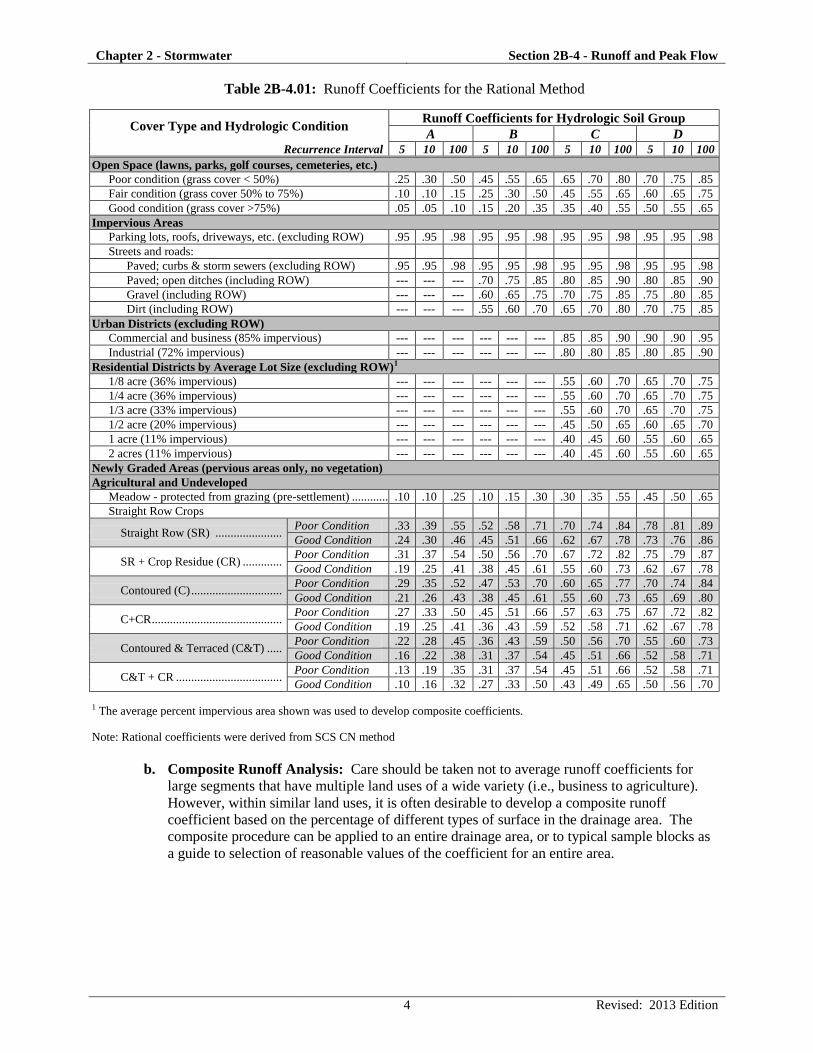
Table 2B-4.01: Runoff Coefficients for the Rational Method

Cover Type and Hydrologic Condition Runoff Coefficients for Hydrologic Soil Group

A B C D

Recurrence Interval 5 10 100 5 10 100 5 10 100 5 10 100

Open Space (lawns, parks, golf courses, cemeteries, etc.)

Poor condition (grass cover < 50%) .25 .30 .50 .45 .55 .65 .65 .70 .80 .70 .75 .85

Fair condition (grass cover 50% to 75%) .10 .10 .15 .25 .30 .50 .45 .55 .65 .60 .65 .75

Good condition (grass cover >75%) .05 .05 .10 .15 .20 .35 .35 .40 .55 .50 .55 .65

Impervious Areas

Parking lots, roofs, driveways, etc. (excluding ROW) .95 .95 .98 .95 .95 .98 .95 .95 .98 .95 .95 .98

Streets and roads:

Paved; curbs & storm sewers (excluding ROW) .95 .95 .98 .95 .95 .98 .95 .95 .98 .95 .95 .98

Paved; open ditches (including ROW) --- --- --- .70 .75 .85 .80 .85 .90 .80 .85 .90

Gravel (including ROW) --- --- --- .60 .65 .75 .70 .75 .85 .75 .80 .85

Dirt (including ROW) --- --- --- .55 .60 .70 .65 .70 .80 .70 .75 .85

Urban Districts (excluding ROW)

Commercial and business (85% impervious) --- --- --- --- --- --- .85 .85 .90 .90 .90 .95

Industrial (72% impervious) --- --- --- --- --- --- .80 .80 .85 .80 .85 .90

Residential Districts by Average Lot Size (excluding ROW)1

1/8 acre (36% impervious) --- --- --- --- --- --- .55 .60 .70 .65 .70 .75

1/4 acre (36% impervious) --- --- --- --- --- --- .55 .60 .70 .65 .70 .75

1/3 acre (33% impervious) --- --- --- --- --- --- .55 .60 .70 .65 .70 .75

1/2 acre (20% impervious) --- --- --- --- --- --- .45 .50 .65 .60 .65 .70

1 acre (11% impervious) --- --- --- --- --- --- .40 .45 .60 .55 .60 .65

2 acres (11% impervious) --- --- --- --- --- --- .40 .45 .60 .55 .60 .65

Newly Graded Areas (pervious areas only, no vegetation)

Agricultural and Undeveloped

Meadow - protected from grazing (pre-settlement) ........................ .10 .10 .25 .10 .15 .30 .30 .35 .55 .45 .50 .65

Straight Row Crops

Straight Row (SR) ...................... Poor Condition .33 .39 .55 .52 .58 .71 .70 .74 .84 .78 .81 .89

Good Condition .24 .30 .46 .45 .51 .66 .62 .67 .78 .73 .76 .86

SR + Crop Residue (CR) ............. Poor Condition .31 .37 .54 .50 .56 .70 .67 .72 .82 .75 .79 .87

Good Condition .19 .25 .41 .38 .45 .61 .55 .60 .73 .62 .67 .78

Contoured (C) .............................. Poor Condition .29 .35 .52 .47 .53 .70 .60 .65 .77 .70 .74 .84

Good Condition .21 .26 .43 .38 .45 .61 .55 .60 .73 .65 .69 .80

C+CR ........................................... Poor Condition .27 .33 .50 .45 .51 .66 .57 .63 .75 .67 .72 .82

Good Condition .19 .25 .41 .36 .43 .59 .52 .58 .71 .62 .67 .78

Contoured & Terraced (C&T) ..... Poor Condition .22 .28 .45 .36 .43 .59 .50 .56 .70 .55 .60 .73

Good Condition .16 .22 .38 .31 .37 .54 .45 .51 .66 .52 .58 .71

C&T + CR ................................... Poor Condition .13 .19 .35 .31 .37 .54 .45 .51 .66 .52 .58 .71

Good Condition .10 .16 .32 .27 .33 .50 .43 .49 .65 .50 .56 .70 1 The average percent impervious area shown was used to develop composite coefficients.

Note: Rational coefficients were derived from SCS CN method

b. Composite Runoff Analysis: Care should be taken not to average runoff coefficients for

large segments that have multiple land uses of a wide variety (i.e., business to agriculture).

However, within similar land uses, it is often desirable to develop a composite runoff

coefficient based on the percentage of different types of surface in the drainage area. The

composite procedure can be applied to an entire drainage area, or to typical sample blocks as

a guide to selection of reasonable values of the coefficient for an entire area.



c. Rainfall Intensity: The intensity (iT) is the average rainfall rate in inches per hour for the

period of maximum rainfall of a given frequency, with duration equal to the time of

concentration. The method(s) for determining time of concentration are presented in Section

2B-3.

From a practical standpoint, using a Tc of less than 15 minutes may yield unreasonably high

flow rates. For most applications, a minimum Tc of 15 minutes may be used.

After the Tc has been determined, the rainfall intensity should be obtained. For the Rational

method, the design rainfall intensity is that which occurs for the design year storm whose

duration equals the time of concentration. Tables 2B-2.02 through 2B-2.10 in Section 2B-2

provide the Iowa rainfall data from Bulletin 71 to allow determination of rainfall intensity

based on duration equaling the time of concentration.

d. Area: The area (A) of the basin in acres. A map showing the limits of the drainage basin

used in design should be provided with design data and will be superimposed on the grading

plan showing subbasins. As mentioned earlier, the configuration of the contributing area with

respect to pervious and impervious sub-areas and the flow path should be considered when

deciding whether to use all or a portion of the total area.

C. SCS Methods

Several methods of determining total runoff and peak runoff have been developed by the SCS (now

known as the NRCS). The two methods described below include the SCS Runoff Curve Number

method for determining the total runoff depth and the SCS Peak flow method, which utilizes the

runoff depth and site conditions to determine the peak rate of runoff from a drainage area.

These methods are described in full detail in the NRCS Technical Release 55: Urban Hydrology for

Small Watersheds. This document is also the basis for the publicly available computer program

WIN-TR55. This section also includes information from the NRCS National Engineering Handbook,

Part 630.

1. SCS Curve Number: The SCS methods classify the land use and soil type by a single parameter

called the Curve Number (CN). The CN can be used to represent the drainage properties for any

sized homogeneous watershed with a known percentage of imperviousness.

The major factors that determine CN are the hydrologic soil group, cover type, treatment,

hydrologic condition, and antecedent runoff condition. Tables 2B-4.03 through 2B-4.05 include

typical CN values for urban and agricultural areas respectively.

Several factors, such as the percentage of impervious area and the means of conveying runoff

from the impervious areas to the drainage system, should be considered in computing the CN for

urban areas. For example, do the impervious areas connect directly to the drainage system, or do

they outlet onto lawns or other pervious areas where infiltration can occur?

The urban CN values (Table 2B-4.03) were developed for typical land use relationships based

upon specific assumed percentages of impervious area. These CN values were developed on the

assumptions that (a) the pervious urban areas are equivalent to pasture in good hydrologic

condition, (b) impervious areas have a CN of 98 and are directly connected to the drainage

system, and (c) the CN values for urban and residential districts assume an average percent

impervious as shown in Table 2B-4.03.



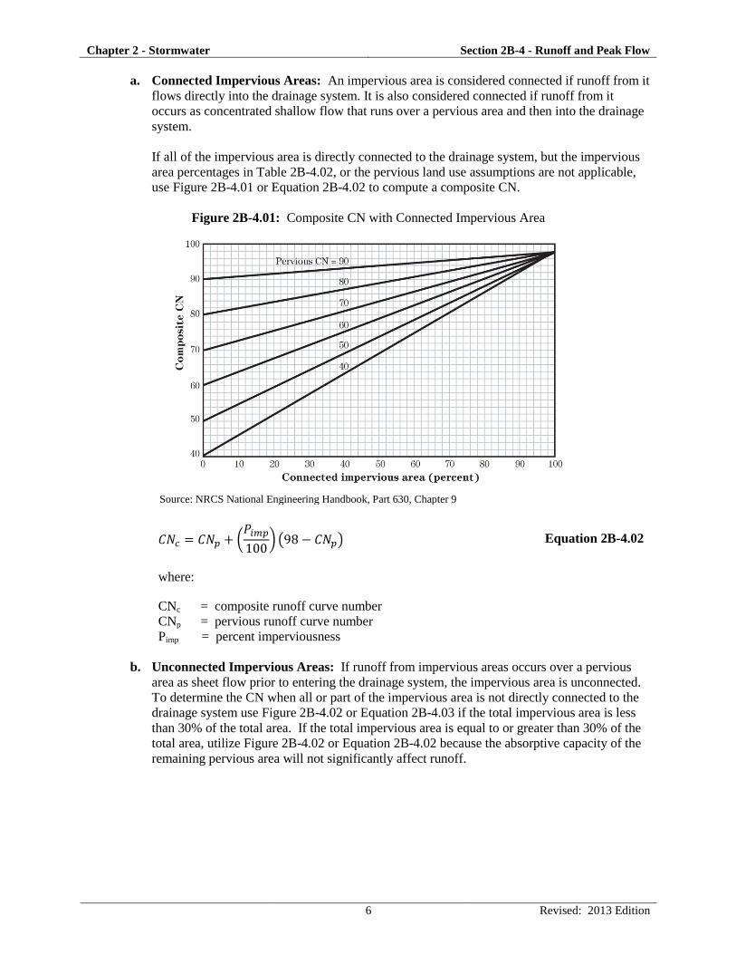
a. Connected Impervious Areas: An impervious area is considered connected if runoff from it

flows directly into the drainage system. It is also considered connected if runoff from it

occurs as concentrated shallow flow that runs over a pervious area and then into the drainage

system.

If all of the impervious area is directly connected to the drainage system, but the impervious

area percentages in Table 2B-4.02, or the pervious land use assumptions are not applicable,

use Figure 2B-4.01 or Equation 2B-4.02 to compute a composite CN.

Figure 2B-4.01: Composite CN with Connected Impervious Area

Source: NRCS National Engineering Handbook, Part 630, Chapter 9

(

) ( ) Equation 2B-4.02

where:

CNc = composite runoff curve number

CNp = pervious runoff curve number

Pimp = percent imperviousness

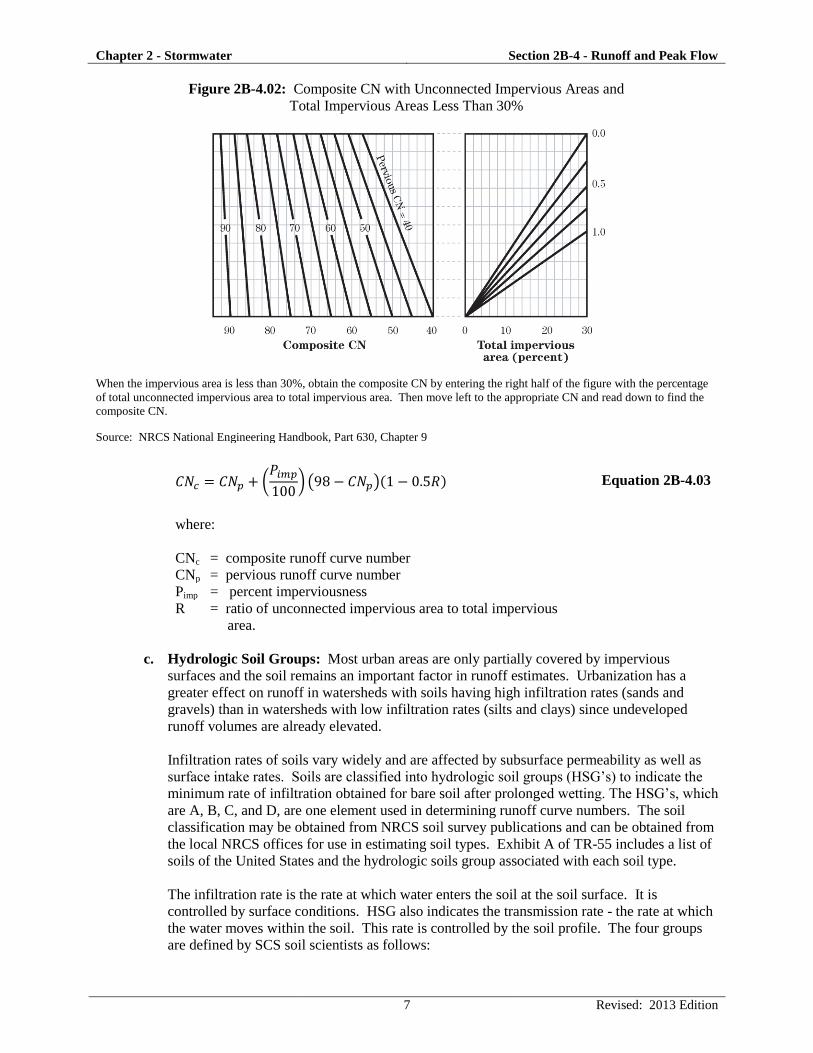
b. Unconnected Impervious Areas: If runoff from impervious areas occurs over a pervious

area as sheet flow prior to entering the drainage system, the impervious area is unconnected.

To determine the CN when all or part of the impervious area is not directly connected to the

drainage system use Figure 2B-4.02 or Equation 2B-4.03 if the total impervious area is less

than 30% of the total area. If the total impervious area is equal to or greater than 30% of the

total area, utilize Figure 2B-4.02 or Equation 2B-4.02 because the absorptive capacity of the

remaining pervious area will not significantly affect runoff.



Figure 2B-4.02: Composite CN with Unconnected Impervious Areas and

Total Impervious Areas Less Than 30%

When the impervious area is less than 30%, obtain the composite CN by entering the right half of the figure with the percentage

of total unconnected impervious area to total impervious area. Then move left to the appropriate CN and read down to find the

composite CN.


(

) ( )( ) Equation 2B-4.03

where:

CNc = composite runoff curve number

CNp = pervious runoff curve number

Pimp = percent imperviousness

R = ratio of unconnected impervious area to total impervious

area.

c. Hydrologic Soil Groups: Most urban areas are only partially covered by impervious

surfaces and the soil remains an important factor in runoff estimates. Urbanization has a

greater effect on runoff in watersheds with soils having high infiltration rates (sands and

gravels) than in watersheds with low infiltration rates (silts and clays) since undeveloped

runoff volumes are already elevated.

Infiltration rates of soils vary widely and are affected by subsurface permeability as well as

surface intake rates. Soils are classified into hydrologic soil groups (HSG’s) to indicate the

minimum rate of infiltration obtained for bare soil after prolonged wetting. The HSG’s, which

are A, B, C, and D, are one element used in determining runoff curve numbers. The soil

classification may be obtained from NRCS soil survey publications and can be obtained from

the local NRCS offices for use in estimating soil types. Exhibit A of TR-55 includes a list of

soils of the United States and the hydrologic soils group associated with each soil type.

The infiltration rate is the rate at which water enters the soil at the soil surface. It is

controlled by surface conditions. HSG also indicates the transmission rate - the rate at which

the water moves within the soil. This rate is controlled by the soil profile. The four groups

are defined by SCS soil scientists as follows:



1) Group A: Group A soils have low runoff potential and high infiltration rates even when

thoroughly wetted. They consist chiefly of deep, well to excessively drained sand or

gravel and have a high rate of water transmission (greater than 0.30 in/hr).

2) Group B: Group B soils have moderate infiltration rates when thoroughly wetted and

consist chiefly of moderately deep to deep, moderately well to well drained soils with

moderately fine to moderately coarse textures. These soils have a moderate rate of water

transmission (0.15 to 0.30 in/hr).

3) Group C: Group C soils have low infiltration rates when thoroughly wetted and consist

chiefly of soils with a layer that impedes downward movement of water and soils with

moderately fine to fine texture. These soils have a low rate of water transmission (0.05 to

0.15 in/hr).

4) Group D: Group D soils have high runoff potential. They have very low infiltration

rates when thoroughly wetted and consist chiefly of clay soils with a high swelling

potential, soils with a permanent high water table, soils with a claypan or clay layer at or

near the surface, and shallow soils over nearly impervious material. These soils have a

very low rate of water transmission (0 to 0.05 in/hr).

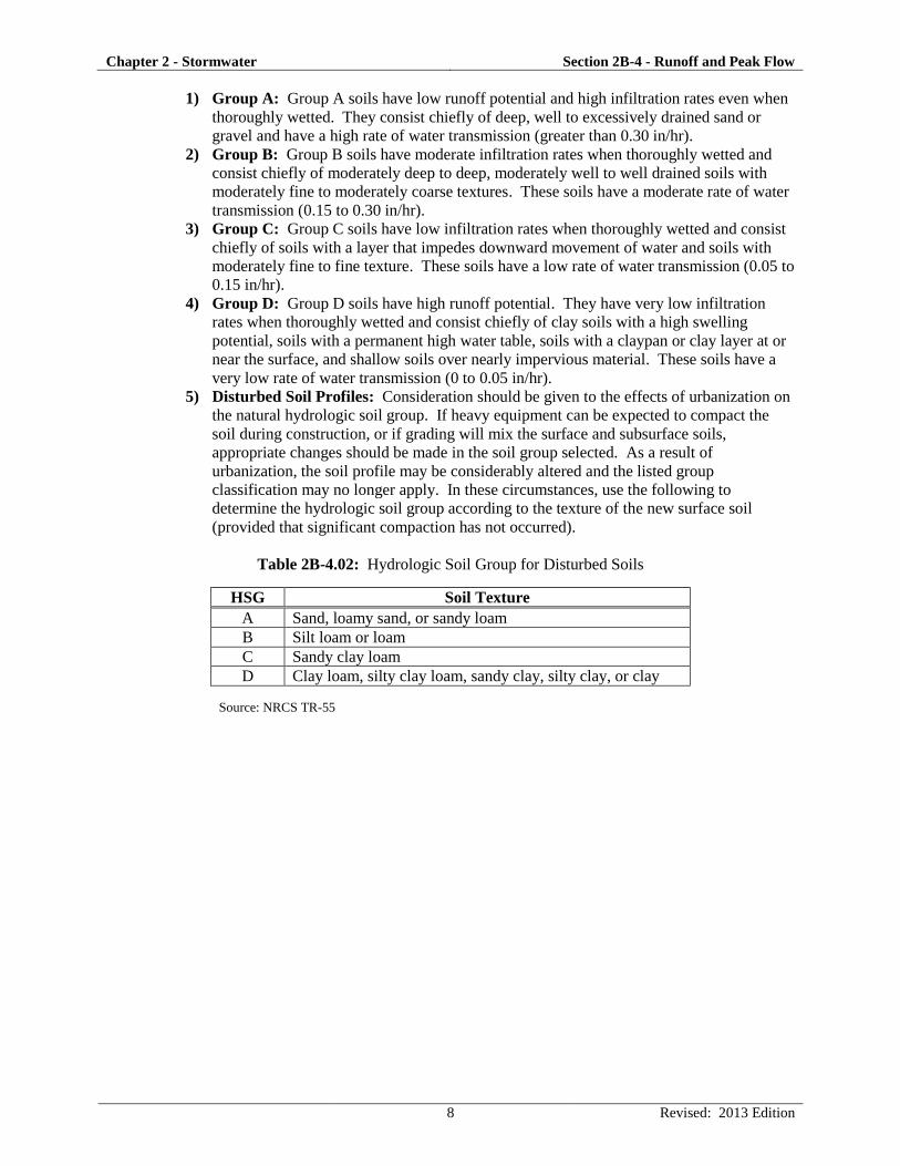
5) Disturbed Soil Profiles: Consideration should be given to the effects of urbanization on

the natural hydrologic soil group. If heavy equipment can be expected to compact the

soil during construction, or if grading will mix the surface and subsurface soils,

appropriate changes should be made in the soil group selected. As a result of

urbanization, the soil profile may be considerably altered and the listed group

classification may no longer apply. In these circumstances, use the following to

determine the hydrologic soil group according to the texture of the new surface soil

(provided that significant compaction has not occurred).

Table 2B-4.02: Hydrologic Soil Group for Disturbed Soils

HSG Soil Texture

A Sand, loamy sand, or sandy loam

B Silt loam or loam

C Sandy clay loam

D Clay loam, silty clay loam, sandy clay, silty clay, or clay

Source: NRCS TR-55



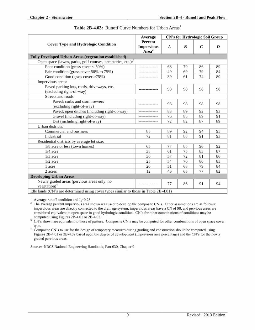
Table 2B-4.03: Runoff Curve Numbers for Urban Areas1

Cover Type and Hydrologic Condition

Average

Percent

Impervious

Area2

CN’s for Hydrologic Soil Group

A B C D

Fully Developed Urban Areas (vegetation established)

Open space (lawns, parks, golf courses, cemeteries, etc.):3

Poor condition (grass cover < 50%) -------------- 68 79 86 89

Fair condition (grass cover 50% to 75%) -------------- 49 69 79 84

Good condition (grass cover >75%) -------------- 39 61 74 80

Impervious areas:

Paved parking lots, roofs, driveways, etc.

(excluding right-of-way) -------------- 98 98 98 98

Streets and roads:

Paved; curbs and storm sewers

(excluding right-of-way) -------------- 98 98 98 98

Paved; open ditches (including right-of-way) -------------- 83 89 92 93

Gravel (including right-of-way) -------------- 76 85 89 91

Dirt (including right-of-way) -------------- 72 82 87 89

Urban districts:

Commercial and business 85 89 92 94 95

Industrial 72 81 88 91 93

Residential districts by average lot size:

1/8 acre or less (town homes) 65 77 85 90 92

1/4 acre 38 61 75 83 87

1/3 acre 30 57 72 81 86

1/2 acre 25 54 70 80 85

1 acre 20 51 68 79 84

2 acres 12 46 65 77 82

Developing Urban Areas

Newly graded areas (pervious areas only, no

vegetation)4

-------------- 77 86 91 94

Idle lands (CN’s are determined using cover types similar to those in Table 2B-4.01)

1 Average runoff condition and Ia=0.2S 2 The average percent impervious area shown was used to develop the composite CN’s. Other assumptions are as follows:

impervious areas are directly connected to the drainage system, impervious areas have a CN of 98, and pervious areas are

considered equivalent to open space in good hydrologic condition. CN’s for other combinations of conditions may be

computed using Figures 2B-4.01 or 2B-4.02. 3 CN’s shown are equivalent to those of pasture. Composite CN’s may be computed for other combinations of open space cover

type. 4 Composite CN’s to use for the design of temporary measures during grading and construction should be computed using

Figures 2B-4.01 or 2B-4.02 based upon the degree of development (impervious area percentage) and the CN’s for the newly

graded pervious areas.




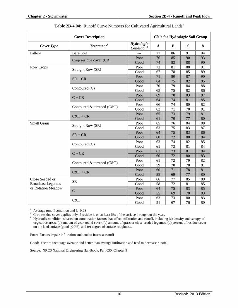
Table 2B-4.04: Runoff Curve Numbers for Cultivated Agricultural Lands1

Cover Description CN’s for Hydrologic Soil Group

Cover Type Treatment2

Hydrologic

Condition3

A B C D

Fallow Bare Soil --- 77 86 91 94

Crop residue cover (CR) Poor 76 85 90 93

Good 74 83 88 90

Row Crops Straight Row (SR)

Poor 72 81 88 91

Good 67 78 85 89

SR + CR Poor 71 80 87 90

Good 64 75 82 85

Contoured (C) Poor 70 79 84 88

Good 65 75 82 86

C + CR Poor 69 78 83 87

Good 64 74 81 85

Contoured & terraced (C&T) Poor 66 74 80 82

Good 62 71 78 81

C&T + CR Poor 65 73 79 81

Good 61 70 77 80

Small Grain Straight Row (SR)

Poor 65 76 84 88

Good 63 75 83 87

SR + CR Poor 64 75 83 86

Good 60 72 80 84

Contoured (C) Poor 63 74 82 85

Good 61 73 81 84

C + CR Poor 62 73 81 84

Good 60 72 80 83

Contoured & terraced (C&T) Poor 61 72 79 82

Good 59 70 78 81

C&T + CR Poor 60 71 78 81

Good 58 69 77 80

Close Seeded or

Broadcast Legumes

or Rotation Meadow

SR Poor 66 77 85 89

Good 58 72 81 85

C Poor 64 75 83 85

Good 55 69 78 83

C&T Poor 63 73 80 83

Good 51 67 76 80 1 Average runoff condition and Ia=0.2S 2 Crop residue cover applies only if residue is on at least 5% of the surface throughout the year. 3 Hydraulic condition is based on combination factors that affect infiltration and runoff, including (a) density and canopy of

vegetative areas, (b) amount of year-round cover, (c) amount of grass or close-seeded legumes, (d) percent of residue cover

on the land surface (good >20%), and (e) degree of surface roughness.

Poor: Factors impair infiltration and tend to increase runoff

Good: Factors encourage average and better than average infiltration and tend to decrease runoff.




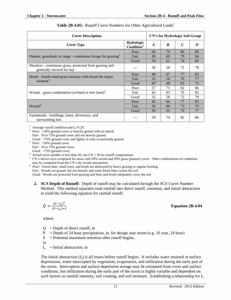
Table 2B-4.05: Runoff Curve Numbers for Other Agricultural Lands1

Cover Description CN’s for Hydrologic Soil Group

Cover Type Hydrologic

Condition3

A B C D

Pasture, grassland, or range - continuous forage for grazing2

Poor 68 79 86 89

Fair 49 69 79 84

Good 39 61 74 80

Meadow - continuous grass, protected from grazing and

generally mowed for hay --- 30 58 71 78

Brush - brush-weed-grass mixture with brush the major

element3

Poor 48 67 77 83

Fair 35 56 70 77

Good 304 48 65 73

Woods - grass combination (orchard or tree farm)5

Poor 57 73 82 86

Fair 43 65 76 82

Good 32 58 72 79

Woods6

Poor 45 66 77 83

Fair 36 60 73 79

Good 30 55 70 77

Farmsteads - buildings, lanes, driveways, and

surrounding lots --- 59 74 82 86

1 Average runoff condition and Ia=0.2S. 2 Poor: <50% ground cover or heavily grazed with no mulch.

Fair: 50 to 75% ground cover and not heavily grazed.

Good: >75% ground cover and lightly or only occasionally grazed. 3 Poor: <50% ground cover.

Fair: 50 to 75% ground cover.

Good: >75% ground cover. 4 Actual curve number is less than 30; use CN = 30 for runoff computations 5 CN’s shown were computed for areas with 50% woods and 50% grass (pasture) cover. Other combinations of conditions

may be computed from the CN’s for woods and pasture. 6 Poor: Forest litter, small trees, and brush are destroyed by heavy grazing or regular burning.

Fair: Woods are grazed, but not burned, and some forest litter covers the soil.

Good: Woods are protected from grazing and litter and brush adequately cover the soil

2. SCS Depth of Runoff: Depth of runoff may be calculated through the SCS Curve Number

Method. This method separates total rainfall into direct runoff, retention, and initial abstraction

to yield the following equation for rainfall runoff.

( )

( ) Equation 2B-4.04

where:

Q = Depth of direct runoff, in

P = Depth of 24 hour precipitation, in. for design year storm (e.g. 10 year, 24 hour)

S = Potential maximum retention after runoff begins,

in

Ia = Initial abstraction, in

The initial abstraction (Ia) is all losses before runoff begins. It includes water retained in surface

depressions, water intercepted by vegetation, evaporation, and infiltration during the early part of

the storm. Interception and surface depression storage may be estimated from cover and surface

conditions, but infiltration during the early part of the storm is highly variable and dependent on

such factors as rainfall intensity, soil crusting, and soil moisture. Establishing a relationship for Ia



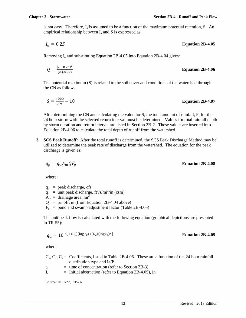
is not easy. Therefore, Ia is assumed to be a function of the maximum potential retention, S. An

empirical relationship between Ia and S is expressed as:

Equation 2B-4.05

Removing Ia and substituting Equation 2B-4.05 into Equation 2B-4.04 gives:

( )

( ) Equation 2B-4.06

The potential maximum (S) is related to the soil cover and conditions of the watershed through

the CN as follows:

Equation 2B-4.07

After determining the CN and calculating the value for S, the total amount of rainfall, P, for the

24 hour storm with the selected return interval must be determined. Values for total rainfall depth

by storm duration and return interval are listed in Section 2B-2. These values are inserted into

Equation 2B-4.06 to calculate the total depth of runoff from the watershed.

3. SCS Peak Runoff: After the total runoff is determined, the SCS Peak Discharge Method may be

utilized to determine the peak rate of discharge from the watershed. The equation for the peak

discharge is given as:

Equation 2B-4.08

where:

qp = peak discharge, cfs

qu = unit peak discharge, ft3/s/mi

2/in (csm)

Am = drainage area, mi2

Q = runoff, in (from Equation 2B-4.04 above)

Fp = pond and swamp adjustment factor (Table 2B-4.05)

The unit peak flow is calculated with the following equation (graphical depictions are presented

in TR-55):

[ ( )( ) ( )( )

] Equation 2B-4.09

where:

C0, C1, C2 = Coefficients, listed in Table 2B-4.06. These are a function of the 24 hour rainfall

distribution type and Ia/P.

tc = time of concentration (refer to Section 2B-3)

Ia = Initial abstraction (refer to Equation 2B-4.05), in

Source: HEC-22, FHWA



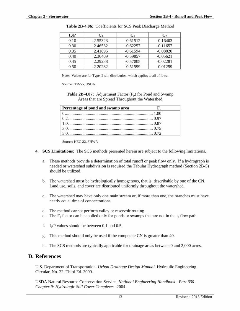
Table 2B-4.06: Coefficients for SCS Peak Discharge Method

Ia/P C0 C1 C2

0.10 2.55323 -0.61512 -0.16403

0.30 2.46532 -0.62257 -0.11657

0.35 2.41896 -0.61594 -0.08820

0.40 2.36409 -0.59857 -0.05621

0.45 2.29238 -0.57005 -0.02281

0.50 2.20282 -0.51599 -0.01259

Note: Values are for Type II rain distribution, which applies to all of Iowa.

Source: TR-55, USDA

Table 2B-4.07: Adjustment Factor (Fp) for Pond and Swamp

Areas that are Spread Throughout the Watershed

Percentage of pond and swamp area Fp

0 ................................................................................. 1.00

0.2 .............................................................................. 0.97

1.0 .............................................................................. 0.87

3.0 .............................................................................. 0.75

5.0 .............................................................................. 0.72

Source: HEC-22, FHWA

4. SCS Limitations: The SCS methods presented herein are subject to the following limitations.

a. These methods provide a determination of total runoff or peak flow only. If a hydrograph is

needed or watershed subdivision is required the Tabular Hydrograph method (Section 2B-5)

should be utilized.

b. The watershed must be hydrologically homogenous, that is, describable by one of the CN.

Land use, soils, and cover are distributed uniformly throughout the watershed.

c. The watershed may have only one main stream or, if more than one, the branches must have

nearly equal time of concentrations.

d. The method cannot perform valley or reservoir routing.

e. The Fp factor can be applied only for ponds or swamps that are not in the tc flow path.

f. Ia/P values should be between 0.1 and 0.5.

g. This method should only be used if the composite CN is greater than 40.

h. The SCS methods are typically applicable for drainage areas between 0 and 2,000 acres.

D. References

U.S. Department of Transportation. Urban Drainage Design Manual. Hydraulic Engineering

Circular, No. 22. Third Ed. 2009.

USDA Natural Resource Conservation Service. National Engineering Handbook - Part 630.

Chapter 9: Hydrologic Soil Cover Complexes. 2004.

Documents

Runoff and Peak Flow - Statewide Urban Design and ... · method provides only an estimate of a single point on the runoff hydrograph). ... Composite Runoff Analysis: ... 2 - Stormwater