1

Toktrapport/Havforskningsinstituttet/ISSN 1503-6294/Nr. 20 - 2004

RV G.O. Sars

MAR-ECO Expedition to the MID-ATLANTIC RIDGE

Leg 2. AZORES - Charlie-Gibbs Fracture Zone.

4 July-5 August 2004

Principal Investigator: Odd Aksel Bergstad, Institute of Marine Research, Norway

Institute of Marine Research and the University of Bergen Bergen, Norway December 2004

2

Please see WWW.MAR-ECO.NO for overall MAR-ECO Science Plan, component

project descriptions, and plans for the RV G.O. Sars expedition 2004. MAR-ECO is a field project of the Census of Marine Life (www.coml.org)

Table of contents 1 Introduction ........................................................................................................................ 2 2 Goals................................................................................................................................... 3 3 Strategies and Methodologies ............................................................................................ 4

3.1 Demersal nekton mapping and sampling. .................................................................. 5 3.2 Zooplankton mapping and process studies, and epibenthos sampling....................... 5 3.3 Abiotic data ................................................................................................................ 9

4 Stations sampled, data and material collected.................................................................... 9 5 Preliminary results............................................................................................................ 12

5.1 Demersal fish catches and observations................................................................... 12 5.2 Cephalopods. ............................................................................................................ 13 5.3 Zooplankton studies ................................................................................................. 22 5.4 UVP-results .............................................................................................................. 22 5.5 Epibenthos................................................................................................................ 28 5.6 Observations by free-fall landers and the ISIT bioluminescence recorder .............. 35 5.7 Physical oceanography............................................................................................. 40

1 Introduction Leg 2 of the MAR-ECO expedition on the RV G.O.Sars started on 4 July 2004 in the afternoon (15:00 Hrs local time) in Horta in the Azores. The schedule for Leg 2 was presented in the cruise plan: Departure Horta: 4 July Arrival Bergen: 4 August Unloading Bergen: 5 August Call at Aberdeen: 3 August During the call in Horta on 3 July crew and scientific personnel for Leg 2 boarded the vessel, and the project organised scientific colloquia, seminars for the Census of Marine Life scientific steering committee, invited guests, schoolchildren, and the media. There was also a social event hosted by MAR-ECO and the Department of Fisheries and Oceanography (DOP) of the University of the Azores, and a formal dinner for invited guests in the Hotel Horta. In the morning of 4 July, the ship was open to the public. The departure from Horta was delayed by late arrival of spare parts for the ROV Bathysaurus. The parts arrived in the morning of 5 July and had then to be fitted and the vehicle tested. The vessel left the harbour of Horta and began steaming towards the first station on 6 July at 01 Hrs. Despite this delay, it was decided to follow the original cruise plan, with the intention to compensate for lost time during the course of the operation.

3

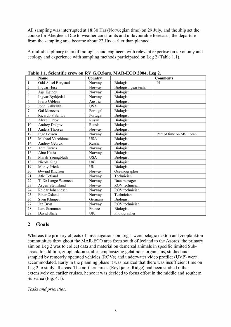
All sampling was interrupted at 18:30 Hrs (Norwegian time) on 29 July, and the ship set the course for Aberdeen. Due to weather constraints and unfavourable forecasts, the departure from the sampling area became about 22 Hrs earlier than planned. A multidisciplinary team of biologists and engineers with relevant expertise on taxonomy and ecology and experience with sampling methods participated on Leg 2 (Table 1.1). Table 1.1. Scientific crew on RV G.O.Sars. MAR-ECO 2004, Leg 2. Name Country Comments 1 Odd Aksel Bergstad Norway Biologist PI 2 Ingvar Huse Norway Biologist, gear tech. 3 Åge Høines Norway Biologist 4 Ingvar Byrkjedal Norway Biologist 5 Franz Uiblein Austria Biologist 6 John Galbraith USA Biologist 7 Gui Menezes Portugal Biologist 8 Ricardo S Santos Portugal Biologist 9 Alexei Orlov Russia Biologist 10 Andrey Dolgov Russia Biologist 11 Anders Thorsen Norway Biologist 12 Inge Fossen Norway Biologist Part of time on MS Loran 13 Michael Vecchione USA Biologist 14 Andrey Gebruk Russia Biologist 15 Tom Sørnes Norway Biologist 16 Aino Hosia Norway Biologist 17 Marsh Youngbluth USA Biologist 18 Nicola King UK Biologist 19 Monty Priede UK Biologist 20 Øyvind Knutsen Norway Oceanographer 21 Atle Totland Norway Technician 22 T. De Lange Wenneck Norway Data manager 23 Asgeir Steinsland Norway ROV technician 24 Reidar Johannesen Norway ROV technician 25 Einar Osland Norway Technician 26 Sven Klimpel Germany Biologist 27 Jan Bryn Norway ROV technician 28 Lars Stemman France Biologist 29 David Shale UK Photographer 2 Goals Whereas the primary objects of investigations on Leg 1 were pelagic nekton and zooplankton communities throughout the MAR-ECO area from south of Iceland to the Azores, the primary aim on Leg 2 was to collect data and material on demersal animals in specific limited Sub-areas. In addition, zooplankton studies emphasizing gelatinous organisms, studied and sampled by remotely operated vehicles (ROVs) and underwater video profiler (UVP) were accommodated. Early in the planning phase it was realized that there was insufficient time on Leg 2 to study all areas. The northern areas (Reykjanes Ridge) had been studied rather extensively on earlier cruises, hence it was decided to focus effort in the middle and southern Sub-area (Fig. 4.1). Tasks and priorities:

4

• To provide data and samples to a range of MAR-ECO component projects, but primarily those focusing on benthopelagic and benthic fauna (Demersal nekton projects DN1, DN2, DN3, DN4), and secondarily the zooplankton components Z1, and Z2.

• To retrieve long-term moorings in southern and middle MAR-ECO sub-areas (moorings deployed during Leg 1).

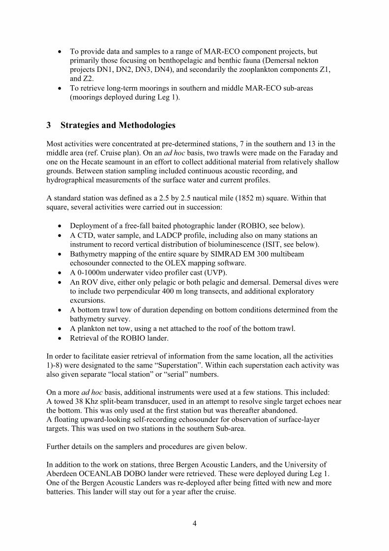
3 Strategies and Methodologies Most activities were concentrated at pre-determined stations, 7 in the southern and 13 in the middle area (ref. Cruise plan). On an ad hoc basis, two trawls were made on the Faraday and one on the Hecate seamount in an effort to collect additional material from relatively shallow grounds. Between station sampling included continuous acoustic recording, and hydrographical measurements of the surface water and current profiles. A standard station was defined as a 2.5 by 2.5 nautical mile (1852 m) square. Within that square, several activities were carried out in succession:

• Deployment of a free-fall baited photographic lander (ROBIO, see below). • A CTD, water sample, and LADCP profile, including also on many stations an

instrument to record vertical distribution of bioluminescence (ISIT, see below). • Bathymetry mapping of the entire square by SIMRAD EM 300 multibeam

echosounder connected to the OLEX mapping software. • A 0-1000m underwater video profiler cast (UVP). • An ROV dive, either only pelagic or both pelagic and demersal. Demersal dives were

to include two perpendicular 400 m long transects, and additional exploratory excursions.

• A bottom trawl tow of duration depending on bottom conditions determined from the bathymetry survey.

• A plankton net tow, using a net attached to the roof of the bottom trawl. • Retrieval of the ROBIO lander.

In order to facilitate easier retrieval of information from the same location, all the activities 1)-8) were designated to the same “Superstation”. Within each superstation each activity was also given separate “local station” or “serial” numbers. On a more ad hoc basis, additional instruments were used at a few stations. This included: A towed 38 Khz split-beam transducer, used in an attempt to resolve single target echoes near the bottom. This was only used at the first station but was thereafter abandoned. A floating upward-looking self-recording echosounder for observation of surface-layer targets. This was used on two stations in the southern Sub-area. Further details on the samplers and procedures are given below. In addition to the work on stations, three Bergen Acoustic Landers, and the University of Aberdeen OCEANLAB DOBO lander were retrieved. These were deployed during Leg 1. One of the Bergen Acoustic Landers was re-deployed after being fitted with new and more batteries. This lander will stay out for a year after the cruise.

5

3.1 Demersal nekton mapping and sampling. General strategy: combination of hydroacoustic mapping, depth-stratified sampling using bottom trawl and ROV observations, along cross-ridge transects in each MAR-ECO box. On Leg 1 of the cruise, semi-quantitative hydroacoustic mapping of demersal (benthopelagic) scatterers was conducted along pre-determined cross-ridge corridors, spanning the depth range from the ridge crest to 3500 m on either side. Zig-zag cruise tracks were surveyed using keel- and hull-mounted transducers (using 5 transmission frequencies). The same was conducted routinely and continuously on Leg 2. Onboard regular scrutinizing of the echosounder (SIMRAD ES 60) recordings was carried out. The main sampler on Leg 2 used to collect depth-stratified nekton samples was a double-warp bottom trawl (Campeln 1800, see details in text box) with associated SCANMAR wireless monitoring instruments. For most tows a downward-looking video camera was fitted to the headline of the trawl. In each sub-area it was an aim to sample down the slope on either side of the ridge to 3500 m. In the middle Sub-area, the plan was to sample a full cross-ridge sequence of stations both south and north of the Charlie-Gibbs Fracture Zone. Deep-sea ROVs were used to provide direct observations and counts of demersal fish and cephalopods, and also epibenthos at selected locations, again depth-stratified. The ROV also provided video footage, but unfortunately not still photos. The ROVs used were produced and operated by Argus Remote Systems (Bergen, Norway) and IMR staff, and two vehicles with a working range to 2000 and 5000m, respectively, were available. Unfortunately, neither vehicle worked satisfactorily for the entire period, so dives were restricted to the depth range 0-2500 m. The vehicle with the deepest range did not operate for more than a few dives, and these were less extensive than planned. Configuration details of the ROVs are given in Table 3.1 and 3.2. Data on near-bottom scavengers (fish and some invertebrates) was obtained by the use of the ROBIO lander provided by the University of Aberdeen OCEANLAB. This free-fall lander collects photographs of fish attracted to a bait throughout a 6-hour period after deployment.

3.2 Zooplankton mapping and process studies, and epibenthos sampling Zooplankton was enumerated and collected by running pelagic transects and exploratory dives using ROV, and by 0-1000m profiles using UVP. The focus was on gelatinous forms, yet the UVP provided more comprehensive data sets. The ROV was fitted with a suction sampler, and the “D-sampler” specially designed for collecting delicate pelagic animals (essentially 4 cylindrical chambers with horizontally movable lids that can be closed when an animal has been teased into the chamber). The D-sampler was provided by the Harbour Branch Oceanographic Institution. Net sampling was not extensive on Leg 2, but a 1m diameter circular net (mesh size) was fitted to the roof of the bottom trawl as a simple device to collect additional animals. This net provided useful samples of some gelatinous animals and also ichthyoplankton. Bioluminescence was recorded by the ISIT provided by the University of Aberdeen OCEANLAB. ISIT is essentially a downward looking video camera filming a screen with a

6

webbing of 1cm mesh. The ISIT was mounted on the CTD-rosette, and as the rosette was lowered through the water column, luminescent organisms would hit the screen and flash. Subsequent analyses of numbers and character of flashes reveals vertical patterns of bioluminescence. Epibenthos sampling included collection of video footage from the ROVs, and sampling of animals from a wide range of taxa caught by the bottom trawl. Equipment applied for demersal trawling

By Ingvar Huse The bottom trawl applied was a Campelen 1800 shrimp trawl, presently used as the standard demersal survey trawl in Norway, northwestern Russia, Canada and Portugal (For a more detailed description, see Engås,1991*). The trawl had four net panels and three bridles. The total distance between the doors and the wing ends was 50 m. Horizontal opening between the upper bridles at the wing tips was 17 m at 50 m doorspread, while the distance between Danlenos at the tips of the ground gear was 12 m. Vertical opening was 4.5 m at 50 m doorspread. The vertical opening was maintained using eight 50 cm diameter plastic encapsulated glass floats evenly spaced along the headrope. The cod-end was equipped with a liner of 22 mm mesh size. The groundgear (rockhopper type, with discs of 35 cm diameter) travelled 3.5 m behind the headrope in the centre of the trawl. There was 10 m of chain as a first part of the lower bridles in front of the Danlenos. According to video recordings made by means of camcorders and lamps in deep water housings attached to the headrope, the rockhoppers travelled within the normally soft substrate, more than halfway submerged, so that most of the fish and epifauna resting on the bottom were caught. Six trawls were brought for the cruise, and two were damaged beyond shipboard repair. Three were torn and fixed on board. The trawl doors used were standard Steinshamn W9 bottom V doors with an area of 6.7 m2 and a weight of 2250 kg. The winch drums held 5000 m of 24 mm wire, which was sufficient for trawling down to 3500 m at 1.5 knots. We could probably have trawled down towards 4000 m with acceptablebottom contact at speeds of around 1.2-1.3 knots. SCANMAR borrowed the project a full suite of newly developed deep-water sensors with reserves for the cruise. These consisted of door spread sensors with depth built in, door angle sensors, depth sensors, temperature sensors, and trawl sounders with ground gear clearance, and headrope distance from the bottom. The door sensors mere adjustable in terms of direction towards the vessel, and angles in three planes calculated by a SCANMAR developed computer program could be set according to the conditions of each haul. Presented on the SCANBAS display the sensors gave a sufficient and generally satisfactory presentation of the trawl geometry during all trawl hauls. A Kongsberg Simrad EM 300 30 kHz 1ox2o multi-beam bottom profiling sounder was applied in the preparatory phase prior to each trawl haul. This sounder provided data for a detailed 3-D mapping of each area, normally with a swat width of around 1.5-2.5 nautical miles. The data could be collected at 5 knots in good weather conditions. Non-processed data were transferred to, and presented on, the Olex navigational plotting system in real time, and detailed 3-D maps of sub-areas at user selected perspective angles and orientations could be readily presented and altered. This tool was an invaluable aid in the planning and documentation of trawl hauls. *Engås, A., 1991. The effects of trawl performance and fish behaviour on the catching efficiency of sampling trawls. Dr. Phil. Thesis, Department of Fisheries and Marine Biology University of Bergen, Norway: 99 pp.

7

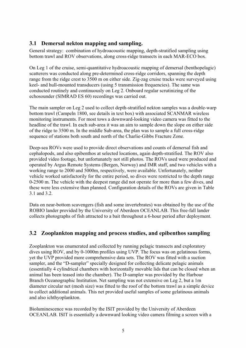
Table 3.1. Specifications of the ROV Aglantha as used on the MAR-ECO Expedition 2004.

Size without tooling skid: Length: 200 cm Width: 125 cm Height: 115 cm Weight: ca. 800 kg Payload: 150 kg Forward/backward speed: 3 knots. Lateral speed: 2 knots. Vertical speed: 2 knots. Depth-rating: 2000 msw Electrical thrusters: 4 x 1,5kW horizontal.

2 x 4 kW vertical. Hydraulics: 1 x Hydraulic powerpack

2 x Hydraulic valvepacks (8 functions) 1 x Hydraulic Pan/Tilt unit 1 x Hydralek 5 function manipulator arm

Camera: 4 x black/white camera.

1 x Colour/Black-white video camera with focus/zoom (Sony EVI-401) Lights: 4 x Halogen lights 500W

4 x HID lights á 150W 4 x IR –lights 2 x Parallel Lasers on the Pan/Tilt for scaling.

Sonar: Mesotech MS1000 (675kHz)

- Tritech Altimeter. - Saiv CTD with salinity, temperature, density, turbidity, oxygen, chlorophyll, - Saiv depthsensor. - KVH FOG Fibre Optical Gyro - KVH C-100 Fluxgate Compass - Roll/Pitch sensor - Simrad MPT324 Transponders used with ship’s Hipap 500 system. Samplers:

- Suction sampler from HBOI with 12 samplers. - 4 x D-samplers from HBOI.

8

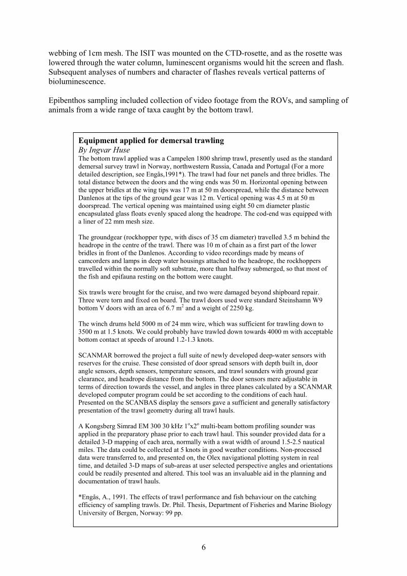
Table 3.2. Specifications of the ROV Bathysaurus as used on the MAR-ECO Expedition 2004.

Size without tooling skid: Length: 170 cm Width: 130 cm Height: 130 cm Weight: ca. 1100 kg Payload: 150 kg Forward/backward speed: 3 knots. Lateral speed: 2 knots. Vertical speed: 2 knots. Depth-rating: 5000 msw Electrical thrusters: 8 x 850W horizontal.

5 x 850W vertical. Hydraulics: 1 x Hydraulic powerpack

1 x Hydraulic valvepack (7 functions) 1 x Hydro-lek 4 function manipulator arm

Camera: 4 x black/white camera.

1 x Colour/Black-white video camera with focus/zoom (Sony FCB-471), controlled via RS-232 with possibility to control Iris and White balance manually.

Lights: 4 x Halogen lights 500W

4 x HID lights á 150W 2 x Parallel Lasers on the Pan/Tilt for scaling.

Sonar: Mesotech MS1000 (675kHz) - Electric pan & Tilt and Tilt unit - Mesotech Altimeter. - Saiv CTD with salinity, temperature, density, turbidity, oxygen, chlorophyll, - Saiv depthsensor. - KVH FOG Fibre Optical Gyro - KVH C-100 Fluxgate Compass - Roll/Pitch sensor - Simrad MPT324 Transponders used with ship’s Hipap 500 system. Samplers:

- Suction sampler from HBOI with 12 samplers. - 4 x D-samplers from HBOI.

9

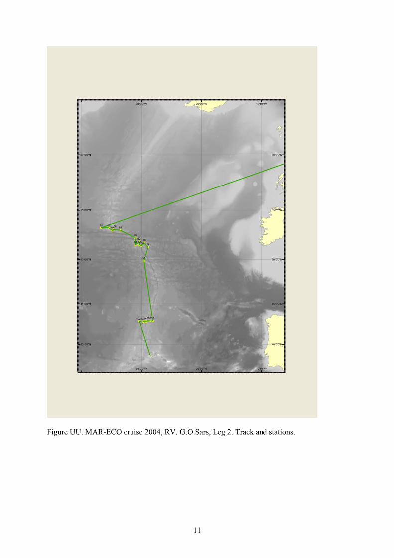
3.3 Abiotic data This included physico-chemical support data in the focus areas, and continuous near-surface sampling along the cruise track. Vertical CTD-casts, current profiling by lowered ADCP, oxygen measurements and sampling of water for nutrient analyses were made regularly in association with sampling activities with e.g. trawls and plankton gear. In addition, continuous recording of hydrographical variables and current profiles was made by ship-mounted instruments (thermosalinograph, ADCP 25-750m). From the Department of Fisheries and Oceanography (DOP), University of the Azores, satellite images of surface temperature were received, mainly as 8-day composites. Charts of the area were inaccurate, hence multi-beam acoustic mapping of focus areas for demersal sampling had to be made to assist the sampling activity and to describe habitats for later analyses. However, the multi-beam echosounder was run continuously, also outside the focus areas. 4 Stations sampled, data and material collected A simplified cruise track and the locations sampled during Leg 2 are shown on Fig. 4.1. Table 4.1 gives details for individual Superstations. In the middle sub-area new locations with similar depths were selected for some stations compared with those given in the cruise plan (M8, 10, 12, 13). This was necessary to save time. One station was skipped (Cruise plan St. M11). The delayed departure from Horta and technical problems with the ROVs introduced time constraints and reduced predictability. There was a frequent need for revision of plans. This resulted in a lot of additional steaming between individual stations within the clusters. Time constraints limited the scope for opportunistic or additional sampling, and the ROV operations became substantially less than planned. The weather was good for most of the period, and only about 1.5 days were lost due to poor working conditions. Due to weather constraints and a problem with the trawl winches on the final day, activities were interrupted about 22 hours earlier than planned, and this resulted in cancellation of the trawl tow and ROV on Supestation 76. A planned repeat dive at Superstation 68 also had to be cancelled for the same reason.

10

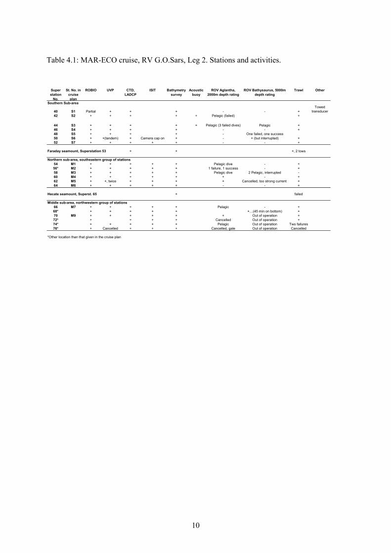
Table 4.1: MAR-ECO cruise, RV G.O.Sars, Leg 2. Stations and activities.

Super station

No.

St. No. in cruise plan

ROBIO UVP CTD, LADCP

ISIT Bathymetry survey

Acoustic buoy

ROV Aglantha, 2000m depth rating

ROV Bathysaurus, 5000m depth rating

Trawl Other

Southern Sub-area

40 S1 Partial + + + - - +Towed

transducer42 S2 + + + + + Pelagic (failed) +

44 S3 + + + + + Pelagic (3 failed dives) Pelagic +46 S4 + + + + - - +48 S5 + + + + - One failed, one success 50 S6 + +(tandem) + Camera cap on + - + (but interrupted) +52 S7 + + + + + - - +

Faraday seamount, Superstation 53 + + +, 2 tows

Northern sub-area, southeastern group of stations54 M1 + + + + + Pelagic dive - +56* M2 + + + + + 1 failure, 1 success - +58 M3 + + + + + Pelagic dive 2 Pelagic, interrupted -60 M4 + + + + + + - +62 M5 + +, twice + + + + Cancelled, too strong current +64 M6 + + + + + - - +

Hecate seamount, Superst. 65 + failed

Middle sub-area, northwestern group of stations66 M7 + + + + + Pelagic - +68* + + + + + +…(45 min on bottom) +70 M9 + + + + + + Out of operation +72* + + + + Cancelled Out of operation +74* + + + + + Pelagic Out of operation Two failures76* + Cancelled + + + Cancelled, gale Out of operation Cancelled

*Other location than that given in the cruise plan

11

Figure UU. MAR-ECO cruise 2004, RV. G.O.Sars, Leg 2. Track and stations.

12

5 Preliminary results.

5.1 Demersal fish catches and observations Uiblein, F., Bergstad, O.A., Byrkjedal, I., Dolgov, A., Fossen, I., Galbraith, J., Hoines, Å., Huse, I., King, N., Klimpel, S., Menezes, G., Orlov, A. & Santos, R.S. The following summarizes the preliminary results of the collections with bottom trawl, and the first results of the observations of demersal fishes with the ROVs Aglantha and Bathysaurus. 1) Results from bottom trawls A total of 22 bottom trawl operations at 18 pre-selected super-stations and the Faraday Seamount were carried out. All of the eight trawl tows in the southern MAR-ECO study box and the two on Faraday Seamount were successful. Of the 12 operations in the middle study box, five of the six tows in the south and all six performed in the north of the Charlie-Gibbs Fracture zone resulted in collection of fishes. The overall depth range covered was 826 to 3505 m. A total of 8335 individual fish of 171 species, 51 families, and 21 orders were collected. However, 456 specimens could only be identified to family level, hence the number of taxa is expected to rise after further work. 88 of the species identified so far belong to pelagic fish families (including all Osmeriformes except for the Alepocephalidae) and 83 to demersal ones. Based on comparison with a list of fishes previously recorded in the investigation area, eight pelagic species (=9.1%) and 21 demersal (=25.3%) were new to the area. Among those new to the area, a single demersal and two pelagic species had been encountered also during Leg1 of the cruise. Potential new species for science were found among the family Ophidiidae of the highly diverse order Ophidiiformes. In particular two specimens of the genus Porogadus collected in the central rift valley of the southern box are candidate new species, as they seemed to differ in morphological characters from other species, including P. miles. However, to arrive at a definitive conclusion further taxonomic studies have to be carried out for this and other potentially new species using comparative material from museum collections. Among the demersal species collected, 47 were encountered in the southern box and 63 in the northern box (including the Faraday Seamount). In pelagic fishes 53 were collected in the south and 49 in the north. Contrasting differences for the two ecological groups were also found by a preliminary multivariate analysis using multidimensional scaling. Whereas pelagic species showed a clear separation in species association patterns between south and north, no such variation occurred in demersals. No patterns were found for both groups when comparing among western and eastern flanks of the ridge. A few demersal fish species showed rather uneven latitudional distribution. In particular the roundnose grenadier Coryphaenoides rupestris occurred only in the northern area where it

13

was dominant in many catches. Another grenadier species, C. brevibarbis, occurred only in the northernmost area north of the Charlie-Gibbs Fracture zone where it also dominated catches. The morid cod Antimora rostrata was only encountered in the middle box and was dominant in two catches. 2) Results from ROV bottom dives Three dives with the ROV Aglantha and four dives with the ROV Bathysaurus provided footage suitable for studies of demersal fishes, and the depth rane of then observations was 789-2355 m. From these seven dives video material representing 24 hrs 33 min in total is available for detailed analyses. In addition, a 51 min sequence deriving from a lander inspection dive with ROV Aglantha on Leg 1can be included. All Leg 2 bottom dives were composed of phases with linear transects over distance of up to 450 m, and exploratory phases. Close-ups during both phases were done to enhance the quality of identifications. At the end of the cruise video material of ca. 7 hrs bottom dive time had been analysed, resulting in the identification of 20 demersal and 5 pelagic fish taxa. Many interesting observations require however further and more detailed analyses, among them the occurrence of mesopelagic fishes at or close to deep sea bottoms indicating possible interaction with these habitats and their fauna. For the second time in all submersible and ROV studies known to us an aggregation of orange roughy Hoplostethus atlanticus (density about 1400 individuals/hectar) was encountered and closely observed. As in former observations in the Bay of Biscay (1600 individuals/hectar) individuals mostly resided inactively close to the bottom, showing both red and white body colouration. For the first time an aggregation of roundnose grenadier was found with an estimated density of between 600 and 700 individuals per hectar. Particularly interesting was that both aggregations were encountered during the same 100 m dive transect, but were spatially segregated. This is a very remarkable finding also for the understanding of biologically relevant scales in the deep-sea. Further working plans include the preparation and storage of the biological material at the Bergen Museum and distribution of the numerous sub-samples for genetic, trophic, and life-history studies. A detailed description and subsequent publication of the very successful deep trawling technique applied during this cruise leg is planned and the acoustic results shall be worked out into detailed to search for evident patterns of demersal fish aggregations. Furthermore, detailed taxonomic studies will be organized to advance with the fish identification work. The video analysis shall be continued. Community analyses shall start as soon as possible and another goal to be reached is the entering of data into OBIS.

5.2 Cephalopods. Michael Vecchione Cephalopods comprise part of the fauna sampled by the pelagic nekton, demersal nekton (and epibenthos), and gelatinous megaplankton components of the MAR-ECO project. However, rather than scattering the reports of the cephalopod fauna among these sub-tasks, these

14

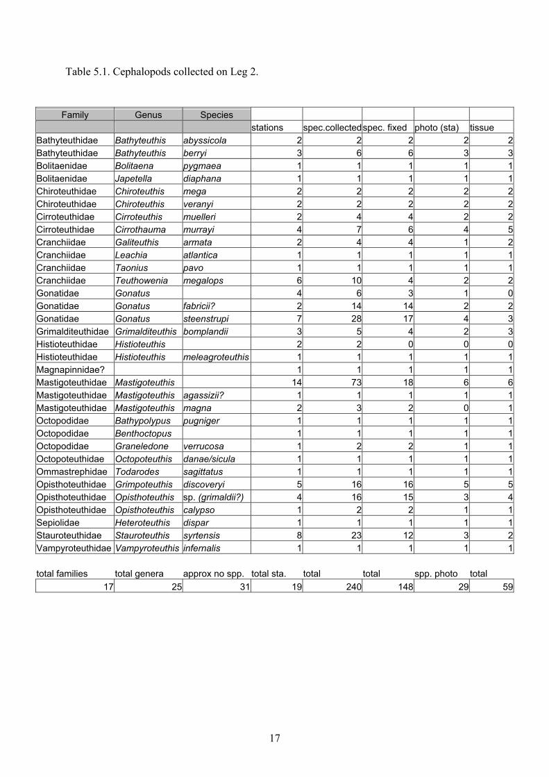
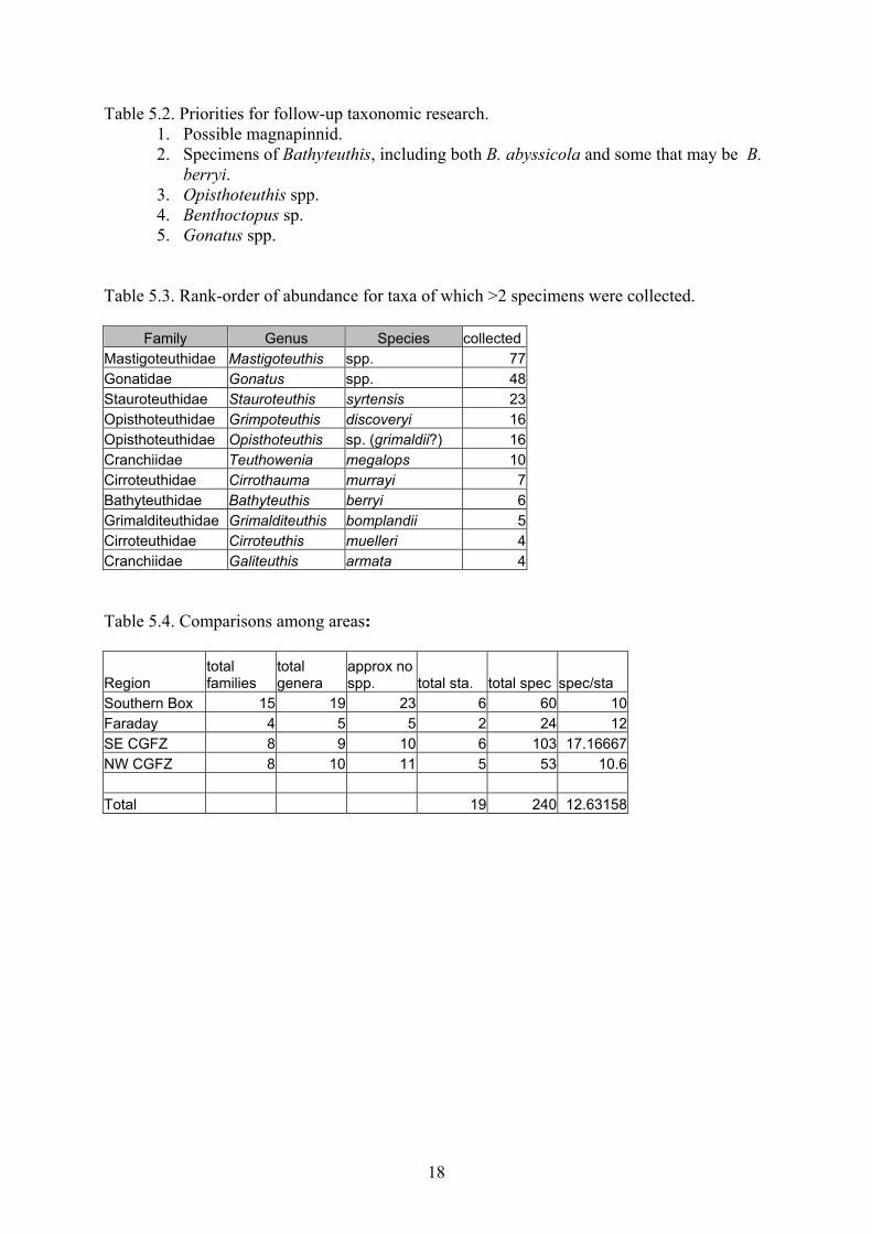
observations are consolidated here into a single section. The results of Leg 2 will be combined with those of Leg 1 for publications on cephalopods of the Mid-Atlantic Ridge. The primary goal of the cephalopod investigation was to explore and to document the diversity of deep-water cephalopods associated with the northern Mid-Atlantic Ridge. The combined results will also contribute to knowledge of distribution and relative abundance, although these observations cannot be considered to be rigorously quantitative. Methods. The strategy for Leg 2 was to record any cephalopod specimens or observations obtained from any operations. The bottom trawl was the primary means of collecting specimens; in addition to the catch in the cod-end, specimens entangled in the mesh of the net were removed and examined. All specimens were identified to the lowest possible taxon and, when the mantle was not too damaged, dorsal mantle length (ML) was measured. Large specimens were weighed as well. Tissue samples were taken and fixed in 96% ethanol for post-cruise analyses of DNA sequences, with the goal of compiling multiple samples from as broad a spectrum of diversity as possible. Digital photographs were taken of the freshly collected whole animals, taxonomic characters, and other anatomical features. Then specimens were selected for fixation in formalin. The fixed specimens are to be transferred to alcohol (either 50% isopropanol or 70% ethanol) at the Bergen Museum for permanent archival. Selection of archival specimens was based on rarity and condition, with preference given to specimens vouchering rare species, taxonomic problems, and tissue samples. Additionally, a few specimens were obtained from the plankton net attached to the headrope of the trawl. Video outputs of all ROV dives were monitored for the presence of cephalopods throughout almost the entire dive, both pelagic and benthic phases. Results. Net Collections. In total, 240 specimens were collected and identified. Of these, 148 were preserved to be archived at the Bergen Museum. Approximately 31 species were included; varying numbers of tissue samples were collected and representative specimens preserved for all distinct types/species (Table 5.1). Among the archival material are several specimens of particular taxonomic interest (Table 5.2). Prime among these is a single specimen of a squid with comparatively huge fins, which may belong to the recently described but poorly known family Magnapinnidae (Vecchione and Young, 1998). Another single specimen of importance is an incirrate octopod of the genus Benthoctopus; the taxonomy of this genus is very confused and this specimen appears to represent a species commonly seen from deep submersibles but for which a valid published name cannot yet be associated. Serious taxonomic problems also exist among four of the eight most common species (Table 5.3). The commonest species encountered was a squid of the family Mastigoteuthidae which, like most mastigoteuthids, was universally damaged by the trawl, including loss of tentacles, skin, and photophores. The loss of these taxonomically important characters precludes confident identification of the species. In the second commonest taxon, Gonatus spp. squids, two species have been described from the North Atlantic. Although most of the specimens of adequate size and condition for confident identification appeared to belong to a single species, G. steenstrupi, a few specimens seemed to have combinations of character states described for G. steenstrupi and G. fabricii. The identity of these specimens and perhaps the status of these two species warrant investigation. In yet another squid genus, Bathyteuthis, only a single species (B. abyssicola) is currently known from the North Atlantic.

15

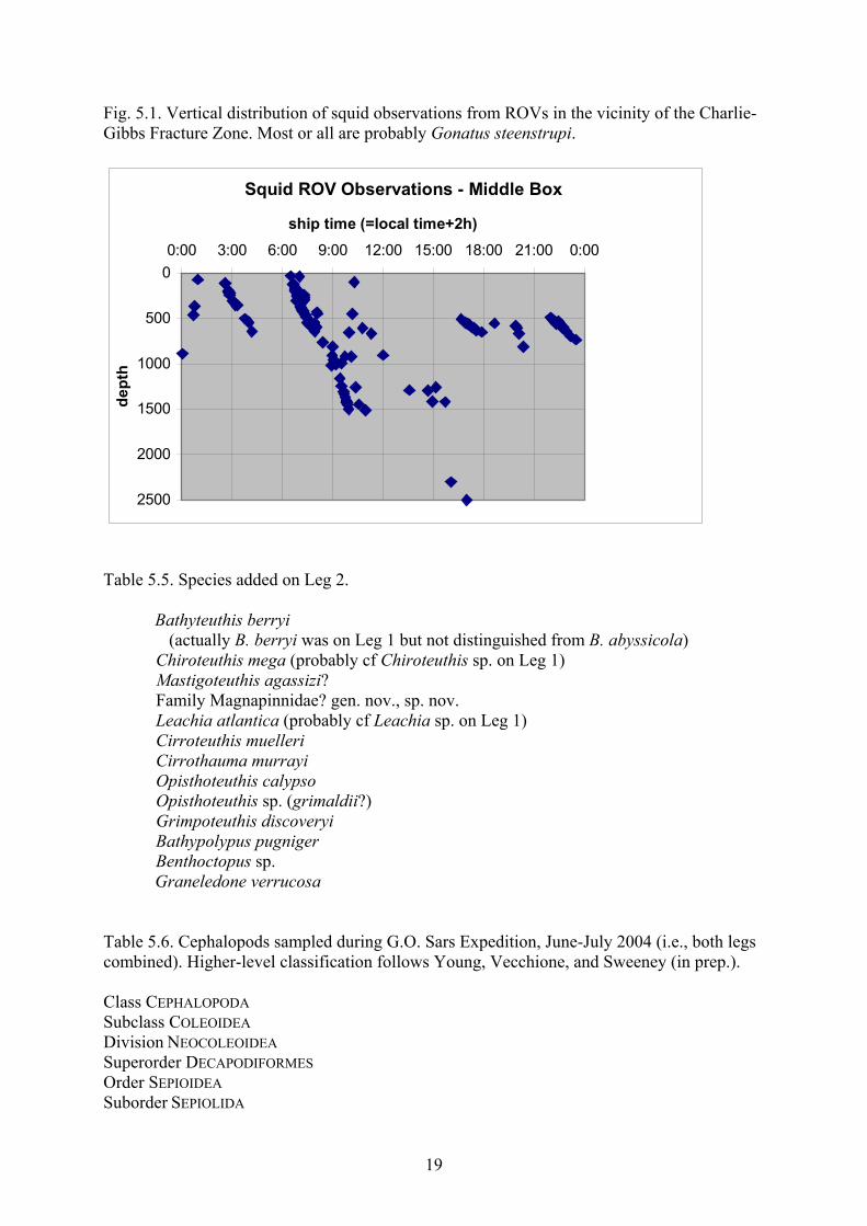
However, most of the Bathyteuthis specimens collected during both legs of this cruise do not fit the taxonomic characters described for B. abyssicola. They are, in fact, more similar to a species known only from the northeastern Pacific Ocean, B. berryi. Finally, specimens of the cirrate octopod genus Opisthoteuthis appear not to match the taxonomic characters of any described Atlantic species. Further study of these specimens is recommended. Five of the ten most commonly collected taxa are cirrate octopods. These large animals appear to be an important component of the benthopelagic and deep bathypelagic nekton of the MAR-ECO study area. The sampling of many specimens in good condition will provide the Bergen Museum with an important collection of Atlantic cirrates. As with many taxonomic groups sampled on this cruise, north-south differences were apparent in the cephalopod fauna (Table 5.4). The highest number of species was collected in the southern box. Conversely, the maximum overall abundance (number collected per trawl) came from farther north, especially from the middle-box transect located southeast of the Charlie-Gibbs Fracture Zone. ROV Observations and Collections. Cephalopod observations from ROV operations can be divided into several categories: (1) multiple squids, (2) single squids, (3) ink only, (4) probable squids. Additionally, two squids were collected by the ROV and a cirrate octopod was observed on one occasion. I consider categories 1 and 2 to represent a higher level of confidence than 3 and 4 and present the numbers below as confident observations+[less confident]. By any measure, dives in the southern MAR-ECO box observed fewer squids (6+[7]) than those on either transect of the middle box. On the southeast transect, 43+[13] observations were recorded, whereas on the northwest transect the total was 55+[22]. Additionally, the cirrate octopod Stauroteuthis syrtensis was observed swimming at 1294 m depth, near bottom at northwest-transect Super Station 70. The observed squids were obviously not mastigoteuthids, which have unique posture and behavior that is recognizable even at a distance (Roper and Vecchione, 1997; Vecchione et al., 2002; Young et al., 1998). All ROV squid observations in the middle box were morphologically consistent with the squids second most common in the trawl samples, Gonatus spp. The squids collected by the ROV were both G. steenstrupi, as were most of the trawl-caught specimens. I therefore assume that most or all of the squid observations in the middle box are that species. Direct observation by submersible allows the time-at-depth for these squids to be known much more precisely than in discrete-depth trawl sampling. Time-at-depth for all squid observations in the middle box is summarized by Fig. 5.1. Almost all observations occurred during the descent phase of the dives. Some interesting patterns are apparent in the presence data. The published depth range for Gonatus spp. in the North Atlantic is from the surface to 1200 m. During these dives, squids were commonly observed at depths down to 1500 m, and occasionally to 2500 m (confident observations). No squids were observed in the upper 1000 m during mid-day, although this interpretation should not be considered to be very rigorous because areas without observations cannot be assumed to indicate absence. Alternative explanations include differential avoidance of the ROV during daylight or lack of sufficient observations during that period. After dark, squids were commonly seen throughout the upper 500 m. These observations should be combined with the discrete-depth midwater trawl results from Leg 1 to provide a better overall picture of vertical distribution and diel migration by G. steenstrupi. The results of Leg 2 add about nine species to the list compiled during Leg 1 (Table 5.5). The additions are primarily cirrate and benthic incirrate octopods. These results also provide possible resolution for some of the unidentified species from the first leg. Pooling the results of this leg with those of Leg 1 results in a preliminary species list of cephalopods in the vicinity of the northern Mid-Atlantic Ridge (Table 5.6). Pending resolution of taxonomic problems, about 53 species were found, representing 43 genera in 29 families. However,

16

because species (and indeed families) were being added right until the end of Leg 2, it is likely that additional sampling would result in the discovery of additional species. Problems and Recommendations. The success of bottom trawling with a large, double-warp otter trawl in this deep and difficult environment actually seem better than expected. As noted above, though, additional sampling, particularly to address both seasonal and inter-annual variability, and bottom trawling in the northern MAR-ECO box are all likely to increase known cephalopod diversity in this area. Conversely, ROV operations could have been much more successful. Additional time in the water, both pelagic and near-bottom, especially at depths >1500 m, would likely have resulted in valuable observations. Cephalopod encounters to be expected in such dives include cirrate octopods, mastigoteuthid squids, and possibly some of the rarely observed and poorly known bathypelagic squids and deep-benthic octopods. References. Roper, C.F.E. and M. Vecchione. 1997. In-situ observations test hypotheses of functional

morphology in Mastigoteuthis. Vie et Milieu 47(2):87-93. Vecchione, M. and R.E. Young. 1998. The Magnapinnidae, a newly discovered family of

oceanic squids (Cephalopoda; Oegopsida). S. Afr. J. Mar. Sci. 20:429-437. Vecchione, M., C.F.E. Roper, E.A. Widder and T.M. Frank. 2002. In-situ observations on

three species of large-finned deep-sea squids. Bull. Mar. Sci. 71(2):893-901. Young, R.E., M. Vecchione, and D.T. Donovan. 1998. The evolution of coleoid cephalopods

and their present biodiversity and ecology. S. Afr. J. Mar. Sci. 20:393-420.

17

Table 5.1. Cephalopods collected on Leg 2.

Family Genus Species stations spec.collectedspec. fixed photo (sta) tissue

Bathyteuthidae Bathyteuthis abyssicola 2 2 2 2 2Bathyteuthidae Bathyteuthis berryi 3 6 6 3 3Bolitaenidae Bolitaena pygmaea 1 1 1 1 1Bolitaenidae Japetella diaphana 1 1 1 1 1Chiroteuthidae Chiroteuthis mega 2 2 2 2 2Chiroteuthidae Chiroteuthis veranyi 2 2 2 2 2Cirroteuthidae Cirroteuthis muelleri 2 4 4 2 2Cirroteuthidae Cirrothauma murrayi 4 7 6 4 5Cranchiidae Galiteuthis armata 2 4 4 1 2Cranchiidae Leachia atlantica 1 1 1 1 1Cranchiidae Taonius pavo 1 1 1 1 1Cranchiidae Teuthowenia megalops 6 10 4 2 2Gonatidae Gonatus 4 6 3 1 0Gonatidae Gonatus fabricii? 2 14 14 2 2Gonatidae Gonatus steenstrupi 7 28 17 4 3Grimalditeuthidae Grimalditeuthis bomplandii 3 5 4 2 3Histioteuthidae Histioteuthis 2 2 0 0 0Histioteuthidae Histioteuthis meleagroteuthis 1 1 1 1 1Magnapinnidae? 1 1 1 1 1Mastigoteuthidae Mastigoteuthis 14 73 18 6 6Mastigoteuthidae Mastigoteuthis agassizii? 1 1 1 1 1Mastigoteuthidae Mastigoteuthis magna 2 3 2 0 1Octopodidae Bathypolypus pugniger 1 1 1 1 1Octopodidae Benthoctopus 1 1 1 1 1Octopodidae Graneledone verrucosa 1 2 2 1 1Octopoteuthidae Octopoteuthis danae/sicula 1 1 1 1 1Ommastrephidae Todarodes sagittatus 1 1 1 1 1Opisthoteuthidae Grimpoteuthis discoveryi 5 16 16 5 5Opisthoteuthidae Opisthoteuthis sp. (grimaldii?) 4 16 15 3 4Opisthoteuthidae Opisthoteuthis calypso 1 2 2 1 1Sepiolidae Heteroteuthis dispar 1 1 1 1 1Stauroteuthidae Stauroteuthis syrtensis 8 23 12 3 2Vampyroteuthidae Vampyroteuthis infernalis 1 1 1 1 1 total families total genera approx no spp. total sta. total total spp. photo total

17 25 31 19 240 148 29 59

18

Table 5.2. Priorities for follow-up taxonomic research. 1. Possible magnapinnid. 2. Specimens of Bathyteuthis, including both B. abyssicola and some that may be B.

berryi. 3. Opisthoteuthis spp. 4. Benthoctopus sp. 5. Gonatus spp.

Table 5.3. Rank-order of abundance for taxa of which >2 specimens were collected.

Family Genus Species collectedMastigoteuthidae Mastigoteuthis spp. 77Gonatidae Gonatus spp. 48Stauroteuthidae Stauroteuthis syrtensis 23Opisthoteuthidae Grimpoteuthis discoveryi 16Opisthoteuthidae Opisthoteuthis sp. (grimaldii?) 16Cranchiidae Teuthowenia megalops 10Cirroteuthidae Cirrothauma murrayi 7Bathyteuthidae Bathyteuthis berryi 6Grimalditeuthidae Grimalditeuthis bomplandii 5Cirroteuthidae Cirroteuthis muelleri 4Cranchiidae Galiteuthis armata 4 Table 5.4. Comparisons among areas:

Region total families

total genera

approx no spp. total sta. total spec spec/sta

Southern Box 15 19 23 6 60 10 Faraday 4 5 5 2 24 12 SE CGFZ 8 9 10 6 103 17.16667 NW CGFZ 8 10 11 5 53 10.6 Total 19 240 12.63158

19

Fig. 5.1. Vertical distribution of squid observations from ROVs in the vicinity of the Charlie-Gibbs Fracture Zone. Most or all are probably Gonatus steenstrupi.

Squid ROV Observations - Middle Box

0

500

1000

1500

2000

2500

0:00 3:00 6:00 9:00 12:00 15:00 18:00 21:00 0:00

ship time (=local time+2h)

dept

h

Table 5.5. Species added on Leg 2.

Bathyteuthis berryi (actually B. berryi was on Leg 1 but not distinguished from B. abyssicola) Chiroteuthis mega (probably cf Chiroteuthis sp. on Leg 1) Mastigoteuthis agassizi? Family Magnapinnidae? gen. nov., sp. nov. Leachia atlantica (probably cf Leachia sp. on Leg 1) Cirroteuthis muelleri Cirrothauma murrayi Opisthoteuthis calypso Opisthoteuthis sp. (grimaldii?) Grimpoteuthis discoveryi Bathypolypus pugniger Benthoctopus sp. Graneledone verrucosa

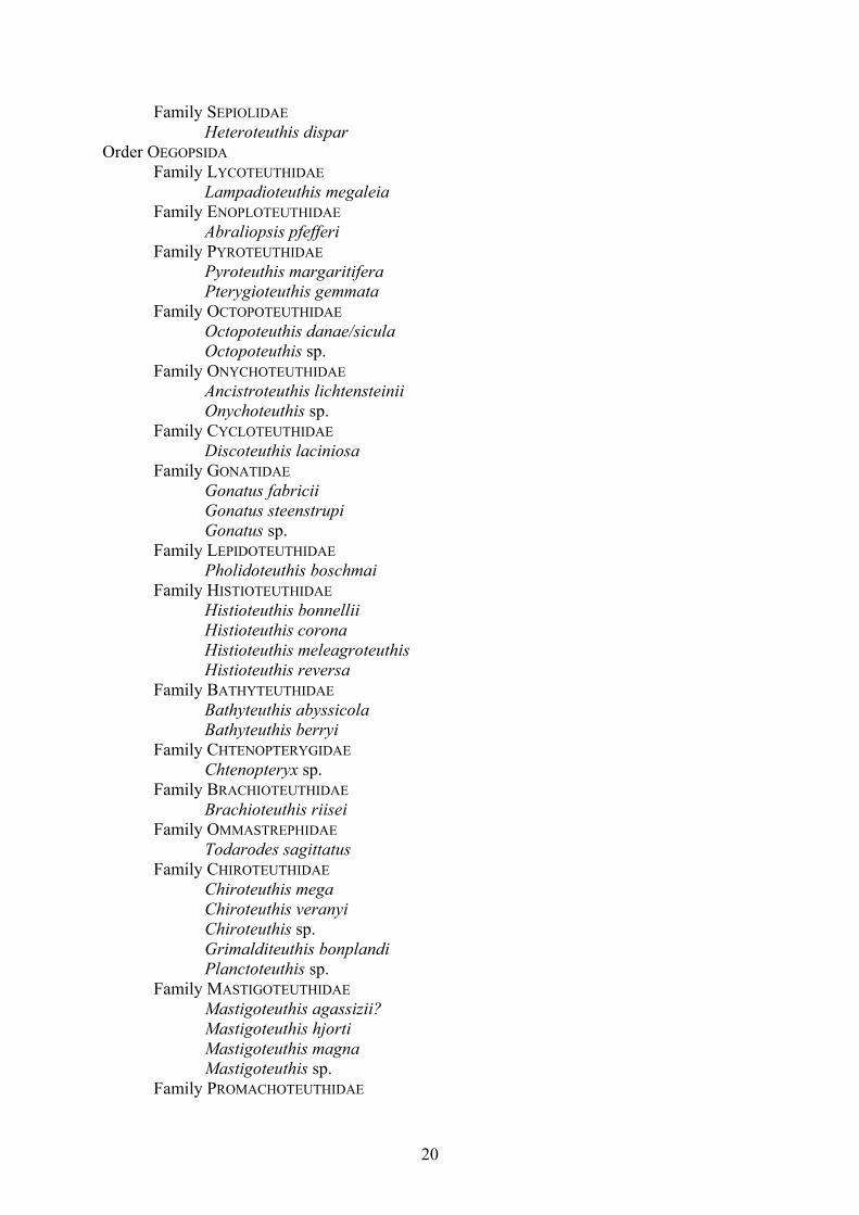
Table 5.6. Cephalopods sampled during G.O. Sars Expedition, June-July 2004 (i.e., both legs combined). Higher-level classification follows Young, Vecchione, and Sweeney (in prep.). Class CEPHALOPODA Subclass COLEOIDEA Division NEOCOLEOIDEA Superorder DECAPODIFORMES Order SEPIOIDEA Suborder SEPIOLIDA

20

Family SEPIOLIDAE Heteroteuthis dispar Order OEGOPSIDA Family LYCOTEUTHIDAE Lampadioteuthis megaleia Family ENOPLOTEUTHIDAE Abraliopsis pfefferi

Family PYROTEUTHIDAE Pyroteuthis margaritifera Pterygioteuthis gemmata Family OCTOPOTEUTHIDAE

Octopoteuthis danae/sicula Octopoteuthis sp. Family ONYCHOTEUTHIDAE Ancistroteuthis lichtensteinii Onychoteuthis sp.

Family CYCLOTEUTHIDAE Discoteuthis laciniosa Family GONATIDAE

Gonatus fabricii Gonatus steenstrupi Gonatus sp. Family LEPIDOTEUTHIDAE Pholidoteuthis boschmai Family HISTIOTEUTHIDAE Histioteuthis bonnellii Histioteuthis corona Histioteuthis meleagroteuthis Histioteuthis reversa Family BATHYTEUTHIDAE Bathyteuthis abyssicola Bathyteuthis berryi Family CHTENOPTERYGIDAE Chtenopteryx sp.

Family BRACHIOTEUTHIDAE Brachioteuthis riisei Family OMMASTREPHIDAE Todarodes sagittatus Family CHIROTEUTHIDAE Chiroteuthis mega

Chiroteuthis veranyi Chiroteuthis sp. Grimalditeuthis bonplandi

Planctoteuthis sp. Family MASTIGOTEUTHIDAE Mastigoteuthis agassizii?

Mastigoteuthis hjorti Mastigoteuthis magna

Mastigoteuthis sp. Family PROMACHOTEUTHIDAE

21

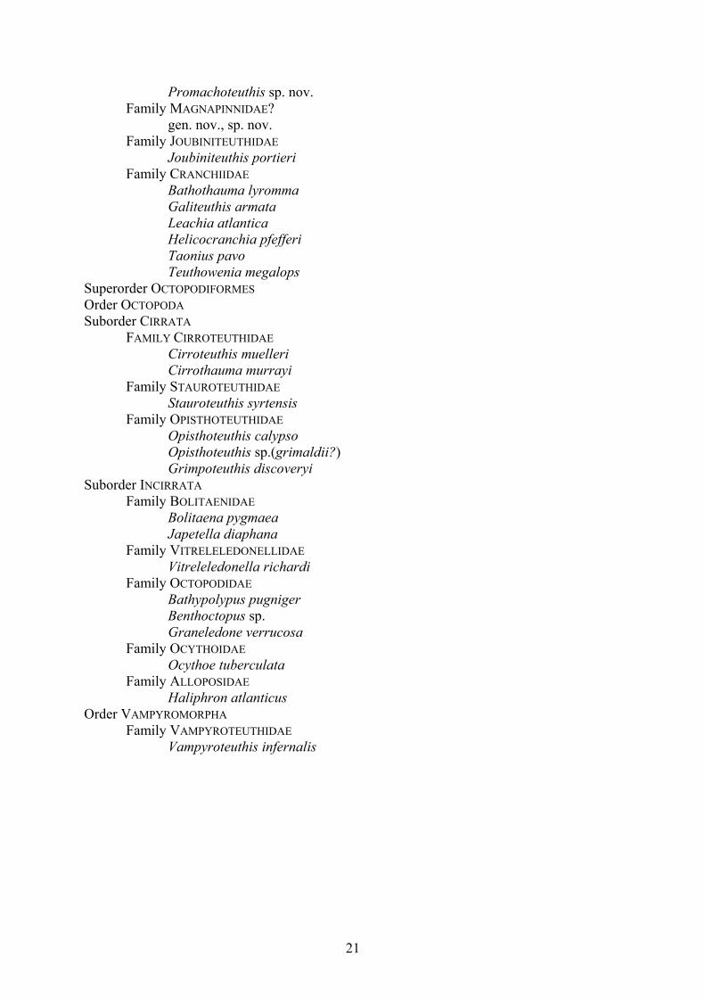
Promachoteuthis sp. nov. Family MAGNAPINNIDAE? gen. nov., sp. nov. Family JOUBINITEUTHIDAE Joubiniteuthis portieri

Family CRANCHIIDAE Bathothauma lyromma

Galiteuthis armata Leachia atlantica

Helicocranchia pfefferi Taonius pavo Teuthowenia megalops Superorder OCTOPODIFORMES Order OCTOPODA Suborder CIRRATA FAMILY CIRROTEUTHIDAE Cirroteuthis muelleri Cirrothauma murrayi Family STAUROTEUTHIDAE Stauroteuthis syrtensis Family OPISTHOTEUTHIDAE Opisthoteuthis calypso Opisthoteuthis sp.(grimaldii?)

Grimpoteuthis discoveryi Suborder INCIRRATA Family BOLITAENIDAE Bolitaena pygmaea Japetella diaphana Family VITRELELEDONELLIDAE Vitreleledonella richardi Family OCTOPODIDAE Bathypolypus pugniger

Benthoctopus sp. Graneledone verrucosa

Family OCYTHOIDAE Ocythoe tuberculata Family ALLOPOSIDAE Haliphron atlanticus Order VAMPYROMORPHA Family VAMPYROTEUTHIDAE Vampyroteuthis infernalis

22

5.3 Zooplankton studies Marsh Youngbluth, Aino Hosia, Tom Sørnes The aims of the zooplankton investigations on Leg 2 were to study the biodiversity, vertical distribution, relative abundance, behavior and metabolism of gelatinous zooplankton at the Mid-Atlantic Ridge. The zooplankton studies on leg 2 relied heavily on the ROVs Bathysaurus and Aglantha, which were used to film the animals in situ as well as to gently capture them and bring them to the surface for further studies with minimal damage. Footage of gelatinous zooplankton distribution in the water column was filmed during the descent to the sea floor on 14 ROV dives. Preliminary analysis suggests that the gelatinous zooplankton in the water column at the study area segregate in layers with regard to depth, with the largest biomass and greatest abundance of animals occurring close to the permanent thermocline, at around 400-800 m. Comparing the results from the ROV footage with those from other sources, such as the UVP and the Multinet, is a task for the post-processing period. The majority of the gelatinous organisms observed were rather small (1-5 cm). A large number of the animals could not be identified to species level from the moving image during the ROV descent and were therefore assigned to a higher taxon only. Several interesting and potentially undescribed gelatinous organisms were seen during the dives but could not be positively identified from the ROV footage alone. Disappointingly, efforts to catch live specimens of these interesting species for further study were largely unsuccessful. The ROVs did, however, facilitate the gentle capture of several specimens of known species for closer investigation and respiration measurements. 15 individuals of the small mesopelagic narcomedusa Aeginura grimaldii were brought to the surface unharmed for estimation of their metabolic rate. Onboard respiration measurements were carried out using a micro-optode system yielding continuous data on the oxygen consumption of the animals. The overall biodiversity of gelatinous zooplankton in the study area seemed to be low, with a higher diversity observed in the southern than in the middle box. A plankton net attached to the bottom trawl allowed a preliminary glimpse into the species composition of gelatinous zooplankton in the region. A total of 47 taxa were identified from the net samples. There are indications that the species composition of gelatinous zooplankton differed between the two study areas: 14 taxa were found exclusively in the Southern box and 13 in the middle box, while 16 taxa occurred throughout the study area. The same plankton net also caught ichthyoplankton, and samples were preserved for subsequent examination.

5.4 UVP-results Lars Stemman The UVP4 has been developed for the acquisition of large-particle (> 60 µm) and zooplankton abundance and size distribution data from 0 to 1000 m. It was designed to minimise the disturbance of the illuminated volume in order to reduce a possible disruption of

23

imaged particles. It is autonomous has been be lowered to 1000m at each station on the hydrological steel cable of the GO SARS. The fourth digital model of the UVP used during MAR-ECO 2004 cruise is described here. The UVP model 4 is a vertically lowered instrument mounted on a galvanized steel frame (1.1 x 0.9 x 1.25 m). The lighting is based on two 54W Chadwick Helmuth stroboscopes. Two mirrors spread the beams into a structured 10 cm thick slab. The strobes are synchronized with two full frame video cameras with 25 and 8 mm C-mount lenses and IR filters. The illuminated particles in a volume of respectively 1.25 and 10.5 liters are recorded simultaneously by the computer. The cameras are positioned perpendicular to the light slab and only illuminated particles in dark background are recorded. The short flash duration (pulse duration = 30 µs) allowed a 1m/s lowering speed without the deterioration of image quality. Depth, temperature and conductivity data are acquired using a Seabird Seacat 19 CTD probe (S/N 1539) with fluorometer and nephelometer (both from Chelsea Instruments Ltd.). The system is powered by four 24V batteries and is piloted by a powerful computer. The data acquisition is time related and programmed prior to the immersion.. The UVP is well adapted to count and measure fragile aggregates such as marine snow as well as delicate zooplankton.

The depth of the images is obtained with the SBE19 probe fixed in the main frame and geographical position by the ships instruments (mainly GPS). Samples consist of computer video files and CTD data. During leg 2, we have performed 19 stations along the mid Atlantic ridge. Nine of them were recorded during the night in order to avoid sun light perturbation on UVP images. All the profiles went down to 1000m (maximum UVP rating) except SuperStation 60 due to the 750 depth of the place. All the UVP data were treated immediately according to our standard procedures to give quasi real-time evaluation of the vertical distributions of particulate matter, CTD data and zooplankton above 5mm (ESD) and copepods above 1mm (ESD). B. PARTICLE PROCESSING The UVP has two important features:

a) it does not disturb the recorded particles or organisms b) b) it allows quick data retrieval and processing.

Processing of images obtained by the UVP in the structured light beam is automated and made by the system during the recovery. The images are analysed and treated automatically by custom-made software. The objects in each image are detected and enumerated. The area and the other parameters of every individual object interesting (measuring above a pre-set size) are measured. Data are stored in an ASCII file and are combined with the associated CTD, fluorometer and nephelometer data (Seasoft Software) using a spreadsheet software. Vertical profiles are printed out onboard immediately after the recovery of the UVP. The results of the calibrations indicate that the tested configuration can detect 60 µm-sized particles and can reliably measure particles larger than 120 µm in diameter. The metric surface as a function of the pixel surface for the 25 mm and 8 mm lens cameras can be expressed by the following equations: Equations for cam0 (X=0) : Sréelle = 0,0024×( Spixels)1,4959

24

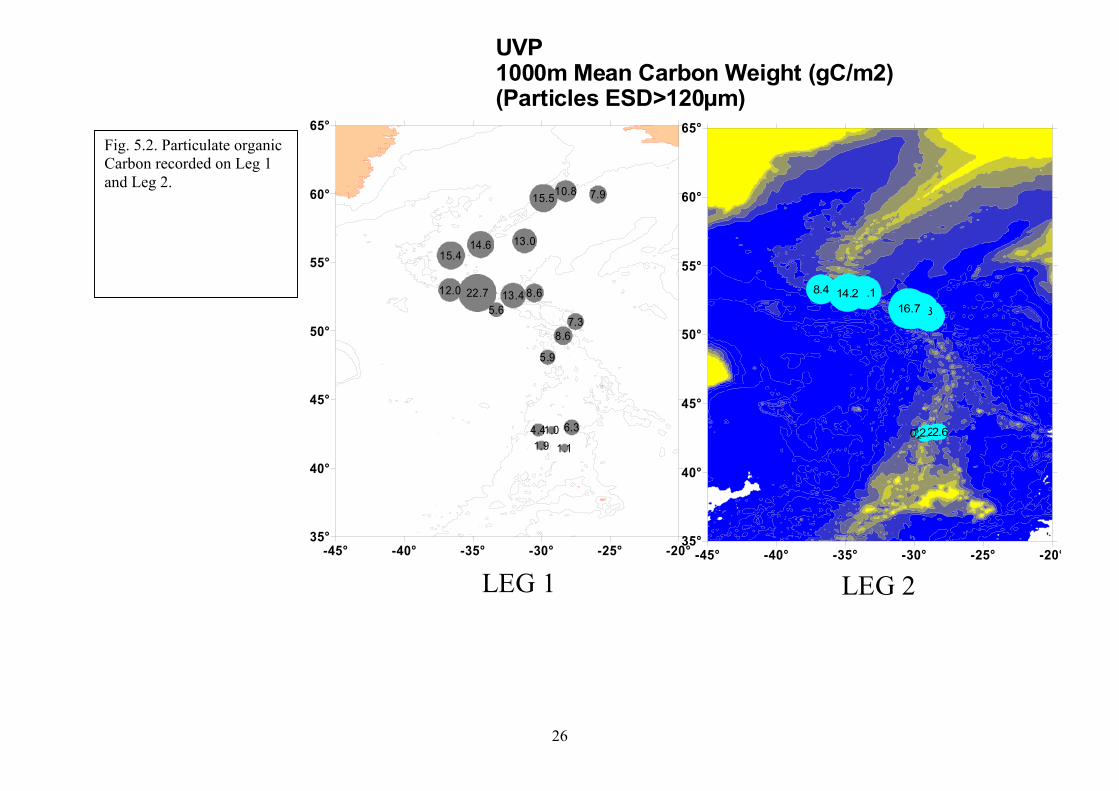
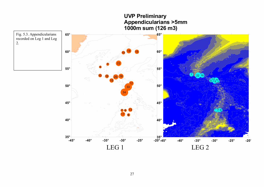
Equations for cam1 (X=1) : Sréelle = 0,0149×( Spixels)1,6128 These equations have to be checked for cross-calibration of both cameras. The calibrations were carried out in a dark test tank filled with 3 m3 filtered (20 µm) sea water. The brightness measured in the test tank was similar to that in the aphotic layers. A calibration grid, placed at different depths of the light slab, was used to estimate the recorded water volume. The dimensions and volume of the parallel light beam recorded by the cameras are : Caméra 25 mm : 14.1 x 10.6 cm Caméra 8 mm : 43.5 x 32.7 cm The pixel/mm relationship was calibrated in a test tank by injection of biological particles (range 40 µm - 20 mm) measured prior to their use with a stereomicroscope (Gorsky et al., Estuarine, Coastal and Shelf Science). C. ZOOPLANKTON PROCESSING We used both Camera 0 and Camera 1 for Zooplankton identification. Camera 0 targets measuring more than 1mm ESD have been visually identified above 200m (and deep to 1000m at some stations) to count large copepodlike bodies. The results are given as total numbers of copepods per 10m of profiles (equivalent to 150L of seawater). Camera 1 targets measuring more than 5 mm ESD and filtered for surface noise due to the sun or on interesting large aggregates have also been manually identified and sorted in major groups : appendic euphaus largedecapod maedusa radiolarians chaetognathe largeaggregates fish thaliacae siphon ctenophore sphere mollusk shapeless otherzoo particle copepodlike diatommatslike. The results are given in total numbers of organisms per 10m of profile (equivalent to 1263 Liters). D. PROBLEMS Lot of targets remains non-identified and will checked by qualified taxonomist after the cruise. Figure 5.2. and 5.3 show examples of outputs from the UVP recordings, comparing data recorded on Leg 1 and Leg 2 of the cruise.

25

26

-45° -40° -35° -30° -25° -20°35°

40°

45°

50°

55°

60°

65°

7.910.815.5

13.014.615.4

22.712.0

5.613.4 8.6

7.38.6

5.9

6.31.04.41.9 1.1

-45° -40° -35° -30° -25° -20°35°

40°

45°

50°

55°

60°

65°

0.81.02.22.72.62.32.6

9.512.85.75.93.812.316.711.112.514.28.88.4

UVP1000m Mean Carbon Weight (gC/m2)(Particles ESD>120µm)

LEG 1 LEG 2

Fig. 5.2. Particulate organic Carbon recorded on Leg 1 and Leg 2.

27

-45° -40° -35° -30° -25° -20°35°

40°

45°

50°

55°

60°

65°

151810

2275

1210

1520 19

1733

34

136717 8

-45° -40° -35° -30° -25° -20°35°

40°

45°

50°

55°

60°

65°

5887 8138

6181689 812162222127

UVP PreliminaryAppendicularians >5mm1000m sum (126 m3)

LEG 1 LEG 2

Fig. 5.3. Appendicularians recorded on Leg 1 and Leg 2.

28

5.5 Epibenthos Andrey V.Gebruk ‘Epibenthos’ is a minor but a separate target of the MAR-ECO project. In the project structure it is designated as a component DN3. On the G.O. Sars MAR-ECO cruise studies of epibenthos were conducted only on Leg 2, from 4 July to 4 August 2004. The main goal of these studies was • to document species diversity of epibenthos in the Mid-Atlantic Ridge area and • to examine the patterns of fauna change along the south-north and east-west gradients in the

Mid-Atlantic Ridge area Strategies and methods. Studies of epibenthos on this cruise included two components:

- sampling of fauna and - observations using ROV

Sampling: Epibenthic organisms were obtained from catches of the fish bottom trawl (Otter Trawl) with the opening 18x4 m. Fauna was first sorted out on deck and then in the lab to the lowest reasonable taxonomical level. Samples were preserved in 80° alcohol or 4% formaldehyde depending on the taxon. Representatives of selected taxa were photographed prior to preservation. Further taxonomical studies of fauna will be conducted on shore by different experts. All collected material will be deposited at the Bergen Museum. ROV observations: The ROVs Aglantha (2000m) and Bathysaurus (5000m) were used for observations both in the water column and at the bottom. Bottom observations were ideally conducted by two pairs of observers (Uiblein/Vecchione and Gebruk/Santos), each working 1.5-2 hours. On each dive video transects and occasional observations with close ups of fauna were planned (see a separate section on ROV observations). Obtained video records will be analysed quantitatively on shore.

Stations sampled Benthic fauna was sampled in total at the following 19 stations: Southern Box: Super Stations 40, 42, 44, 46, 48, 50 and 52.

29

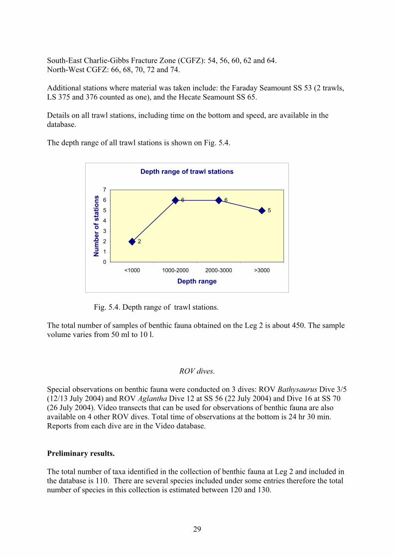
South-East Charlie-Gibbs Fracture Zone (CGFZ): 54, 56, 60, 62 and 64. North-West CGFZ: 66, 68, 70, 72 and 74. Additional stations where material was taken include: the Faraday Seamount SS 53 (2 trawls, LS 375 and 376 counted as one), and the Hecate Seamount SS 65. Details on all trawl stations, including time on the bottom and speed, are available in the database. The depth range of all trawl stations is shown on Fig. 5.4.

Fig. 5.4. Depth range of trawl stations. The total number of samples of benthic fauna obtained on the Leg 2 is about 450. The sample volume varies from 50 ml to 10 l.

ROV dives. Special observations on benthic fauna were conducted on 3 dives: ROV Bathysaurus Dive 3/5 (12/13 July 2004) and ROV Aglantha Dive 12 at SS 56 (22 July 2004) and Dive 16 at SS 70 (26 July 2004). Video transects that can be used for observations of benthic fauna are also available on 4 other ROV dives. Total time of observations at the bottom is 24 hr 30 min. Reports from each dive are in the Video database. Preliminary results. The total number of taxa identified in the collection of benthic fauna at Leg 2 and included in the database is 110. There are several species included under some entries therefore the total number of species in this collection is estimated between 120 and 130.

Depth range of trawl stations

2

6 6

5

0

1

2

3

4

5

6

7

<1000 1000-2000 2000-3000 >3000

Depth range

Num

ber o

f sta

tions

30

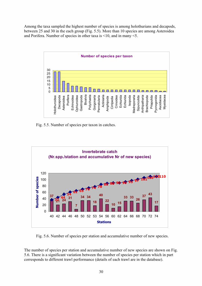
Among the taxa sampled the highest number of species is among holothurians and decapods, between 25 and 30 in the each group (Fig. 5.5). More than 10 species are among Asteroidea and Porifera. Number of species in other taxa is <10, and in many <5.

Fig. 5.5. Number of species per taxon in catches.

Fig. 5.6. Number of species per station and accumulative number of new species.

The number of species per station and accumulative number of new species are shown on Fig. 5.6. There is a significant variation between the number of species per station which in part corresponds to different trawl performance (details of each trawl are in the database).

Number of species per taxon

05

1015202530

Hol

othu

roid

eaD

ecap

oda

Aste

roid

ea

Por

ifera

Echi

noid

eaO

phiu

roid

eaG

astro

poda

Biva

lvia

Poly

chae

taG

orgo

naria

Penn

atul

aria

Actin

iaria

Amph

ipod

a C

irrip

edia

C

rinoi

dea

Echi

urid

aEc

hiur

ida

Isop

oda

Mad

repo

raria

Sipu

ncul

ida

Anth

ipat

haria

Brac

hiop

oda

Pria

pulid

aPy

cnog

onid

aAs

cidi

acea

Mys

idac

ea

Invertebrate catch(Nr.spp./station and accumulative Nr of new species)

3721 24 31

7

34 3418

4022

10 1533 33 26

37 43

1737

4454

61 65 70 74 7885 88 90 90 93 97 101106110110

0

20

40

60

80

100

120

40 42 44 46 48 50 52 53 54 56 60 62 64 66 68 70 72 74

Stations

Nu

mbe

r of

spe

cies

31

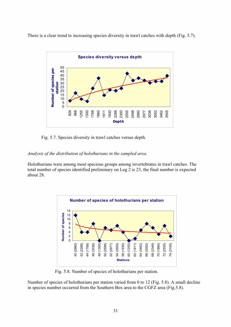
There is a clear trend to increasing species diversity in trawl catches with depth (Fig. 5.7).

Fig. 5.7. Species diversity in trawl catches versus depth. Analysis of the distribution of holothurians in the sampled area. Holothurians were among most specious groups among invertebrates in trawl catches. The total number of species identified preliminary on Leg 2 is 23, the final number is expected about 28.

Fig. 5.8. Number of species of holothurians per station. Number of species of holothurians per station varied from 0 to 12 (Fig. 5.8). A small decline in species number occurred from the Southern Box area to the CGFZ area (Fig.5.8).

Species diversity versus depth

05

101520253035404550

826

966

1255

1300

1768

1860

1911

1930

2288

2300

2555

2598

2960

2977

3036

3052

3462

3505

Depth

Nu

mbe

r of

spe

cies

per

st

atio

n

Number of species of holothurians per station

02468

101214

40 (2

960)

42 (2

288)

44 (1

768)

46 (3

036)

48 (1

300)

50 (2

588)

52 (2

977)

54 (3

505)

56 (1

930)

60 (1

255)

62 (1

911)

64 (3

462)

66 (3

052)

68 (2

349)

70 (1

860)

72 (2

555)

74 (3

100)

Stations

Num

ber o

f spe

cies

32

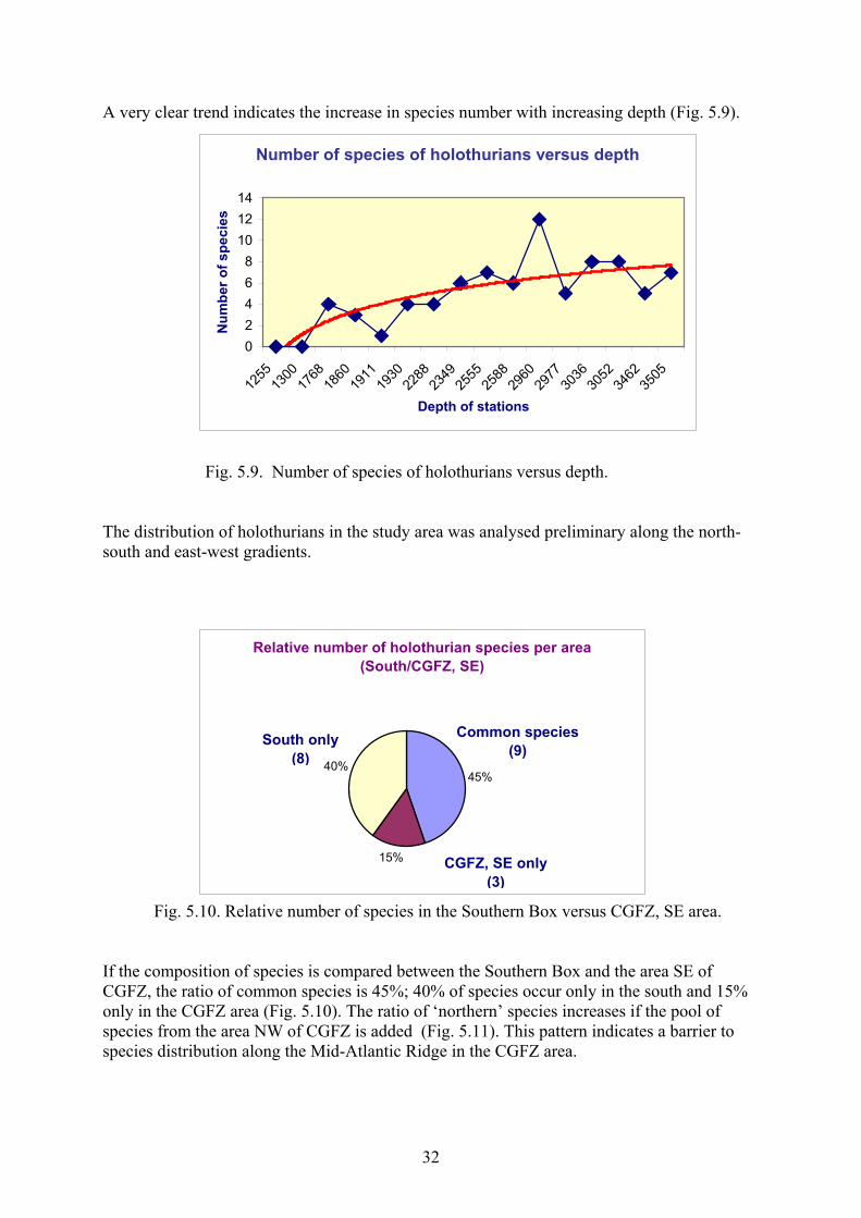
A very clear trend indicates the increase in species number with increasing depth (Fig. 5.9).

Fig. 5.9. Number of species of holothurians versus depth. The distribution of holothurians in the study area was analysed preliminary along the north-south and east-west gradients.

Fig. 5.10. Relative number of species in the Southern Box versus CGFZ, SE area. If the composition of species is compared between the Southern Box and the area SE of CGFZ, the ratio of common species is 45%; 40% of species occur only in the south and 15% only in the CGFZ area (Fig. 5.10). The ratio of ‘northern’ species increases if the pool of species from the area NW of CGFZ is added (Fig. 5.11). This pattern indicates a barrier to species distribution along the Mid-Atlantic Ridge in the CGFZ area.

Relative number of holothurian species per area(South/CGFZ, SE)

15%

40%45%

Common species(9)

South only (8)

CGFZ, SE only(3)

Number of species of holothurians versus depth

02468

101214

1255

1300

1768

1860

1911

1930

2288

2349

2555

2588

2960

2977

3036

3052

3462

3505

Depth of stations

Num

ber o

f spe

cies

33

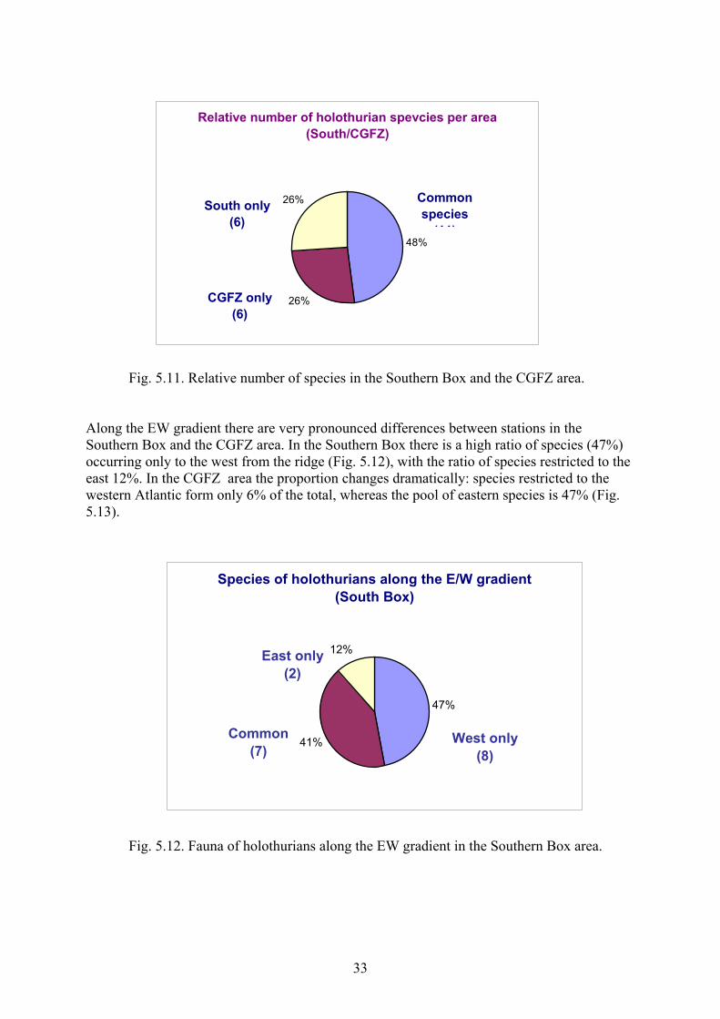
Fig. 5.11. Relative number of species in the Southern Box and the CGFZ area. Along the EW gradient there are very pronounced differences between stations in the Southern Box and the CGFZ area. In the Southern Box there is a high ratio of species (47%) occurring only to the west from the ridge (Fig. 5.12), with the ratio of species restricted to the east 12%. In the CGFZ area the proportion changes dramatically: species restricted to the western Atlantic form only 6% of the total, whereas the pool of eastern species is 47% (Fig. 5.13).

Fig. 5.12. Fauna of holothurians along the EW gradient in the Southern Box area.

Relative number of holothurian spevcies per area(South/CGFZ)

48%

26%

26% Common species

(11)

South only(6)

CGFZ only(6)

Species of holothurians along the E/W gradient(South Box)

47%

41%

12%

West only (8)

Common (7)

East only (2)

34

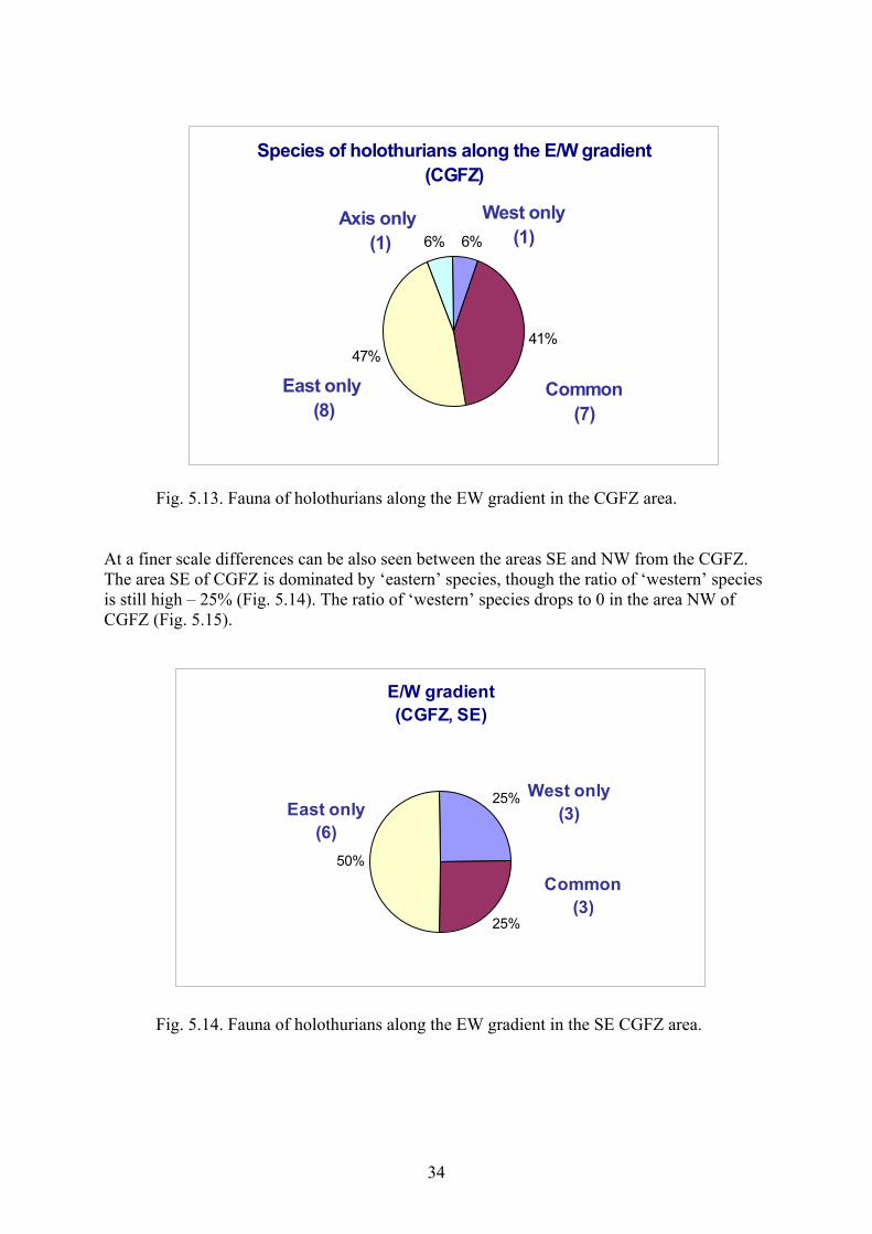
Fig. 5.13. Fauna of holothurians along the EW gradient in the CGFZ area. At a finer scale differences can be also seen between the areas SE and NW from the CGFZ. The area SE of CGFZ is dominated by ‘eastern’ species, though the ratio of ‘western’ species is still high – 25% (Fig. 5.14). The ratio of ‘western’ species drops to 0 in the area NW of CGFZ (Fig. 5.15).

Fig. 5.14. Fauna of holothurians along the EW gradient in the SE CGFZ area.

Species of holothurians along the E/W gradient(CGFZ)

6%

41%47%

6%

East only (8)

Common (7)

West only (1)

Axis only (1)

E/W gradient(CGFZ, SE)

25%

25%

50%

West only (3)

Common (3)

East only (6)

35

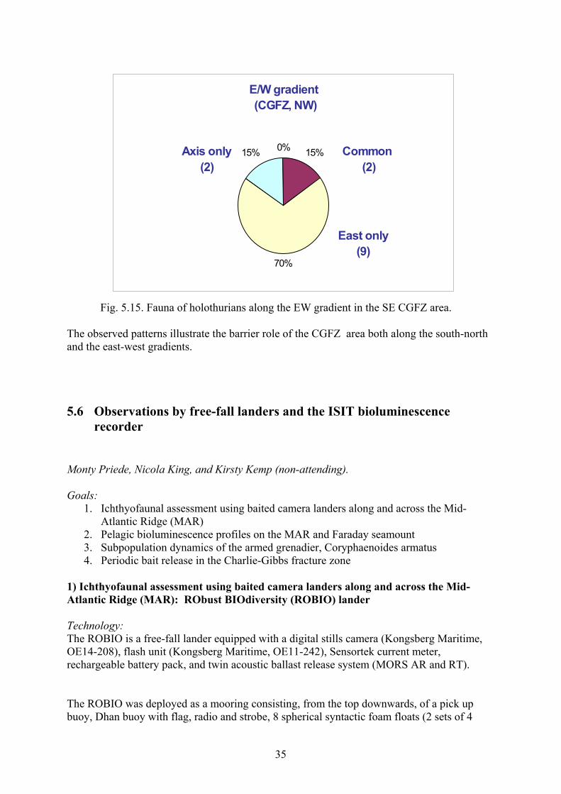
Fig. 5.15. Fauna of holothurians along the EW gradient in the SE CGFZ area.

The observed patterns illustrate the barrier role of the CGFZ area both along the south-north and the east-west gradients.

5.6 Observations by free-fall landers and the ISIT bioluminescence recorder

Monty Priede, Nicola King, and Kirsty Kemp (non-attending). Goals:

1. Ichthyofaunal assessment using baited camera landers along and across the Mid-Atlantic Ridge (MAR)

2. Pelagic bioluminescence profiles on the MAR and Faraday seamount 3. Subpopulation dynamics of the armed grenadier, Coryphaenoides armatus 4. Periodic bait release in the Charlie-Gibbs fracture zone

1) Ichthyofaunal assessment using baited camera landers along and across the Mid-Atlantic Ridge (MAR): RObust BIOdiversity (ROBIO) lander Technology: The ROBIO is a free-fall lander equipped with a digital stills camera (Kongsberg Maritime, OE14-208), flash unit (Kongsberg Maritime, OE11-242), Sensortek current meter, rechargeable battery pack, and twin acoustic ballast release system (MORS AR and RT). The ROBIO was deployed as a mooring consisting, from the top downwards, of a pick up buoy, Dhan buoy with flag, radio and strobe, 8 spherical syntactic foam floats (2 sets of 4

E/W gradient (CGFZ, NW)

0% 15%

70%

15%

East only (9)

Common (2)

Axis only (2)

36

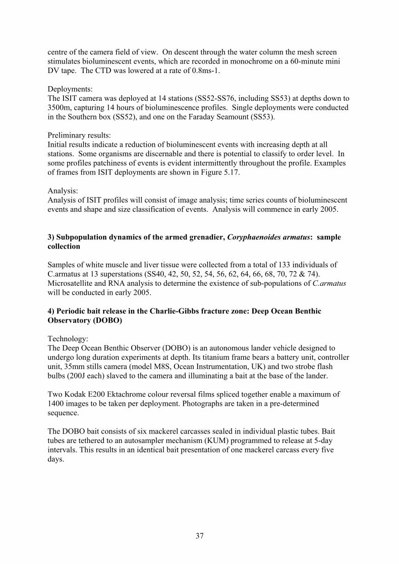
separated by 10m; CRP Marine), 2 glass spheres (Benthos), ROBIO frame, cross reference scale and 95Kg of ballast. When deployed ROBIO descends to the sea floor at 36 m.min-1. The ballast is suspended 2m below the frame of the lander anchoring the mooring, with the reference cross and bait (500g mackerel) attached. The reference scale is situated in the centre of the field of view (1m x 1m cross with 10cm graduated intervals) approximately 20-50cm above the seafloor (dependant on sinkage). Ribbons are attached to the end of each arm to indicate current direction. The camera was programmed to take digital photographs at 90-second intervals, with an average of 250 photos per deployment. The current meter was programmed to measure depth, temperature, current speed and direction and conductivity at one minute intervals throughout the deployment. On deployment completion the ROBIO was released from the ballast by acoustic command from a MORS deck unit via a transponder lowered into the water. The lander therefore returning to the surface by virtue of positive buoyancy. Deployments: The ROBIO lander was deployed at all 19 Super Stations (SS42–SS76). Images were not captured at SS42 due to camera programming problems, deployment 2 at SS44 captured images but due to intermittent autofocus failure the image capture sequence was not consistent. Therefore a total of 17 fully successful deployments were achieved at SS46–SS76. Capturing in excess of 4100 images, at depths ranging from 1012–3508m. Preliminary results: A total of 18 ichthyofaunal species were observed attending the bait, 13 in the Southern box, 11 in the South Eastern cluster of the Middle box and 15 in the North Western cluster. There are a total of 10 species common to both the Southern and Middle boxes. Dominant species attending bait appear to be highly specific to depth strata, with Antimora rostrata and Hydrolagus affinis being the most common species at depths 1500-2500m in both the Southern and Middle boxes. Occurrences of Etmopterus princeps were more prevalent within this depth range in the Southern box. Consistent dominant species at depths exceeding 2500m are Coryphaenoides armatus and Histiobranchus bathybius. Examples of photographs from different deployments are shown in Fig. 5.16. Analysis: Analysis of the ROBIO data will consist of a) image analysis; simple time series counts, length frequency determination, bait visitation by individuals, abundance estimate calculation, confirmation of species identification, behavioural observations, and b) collation and interpretation of current meter data. 2) Pelagic bioluminescence profiles on the MAR and Faraday seamount: Intensified Silicon Intensifier Target (ISIT) camera Technology: The ISIT camera was mounted in profile on the CTD profiler frame (University of Bergen), with a mesh screen, Barium LED and controller unit to interface camera and power, and to provide data storage. The mesh screen was located 60cm from the camera faceplate in the

37

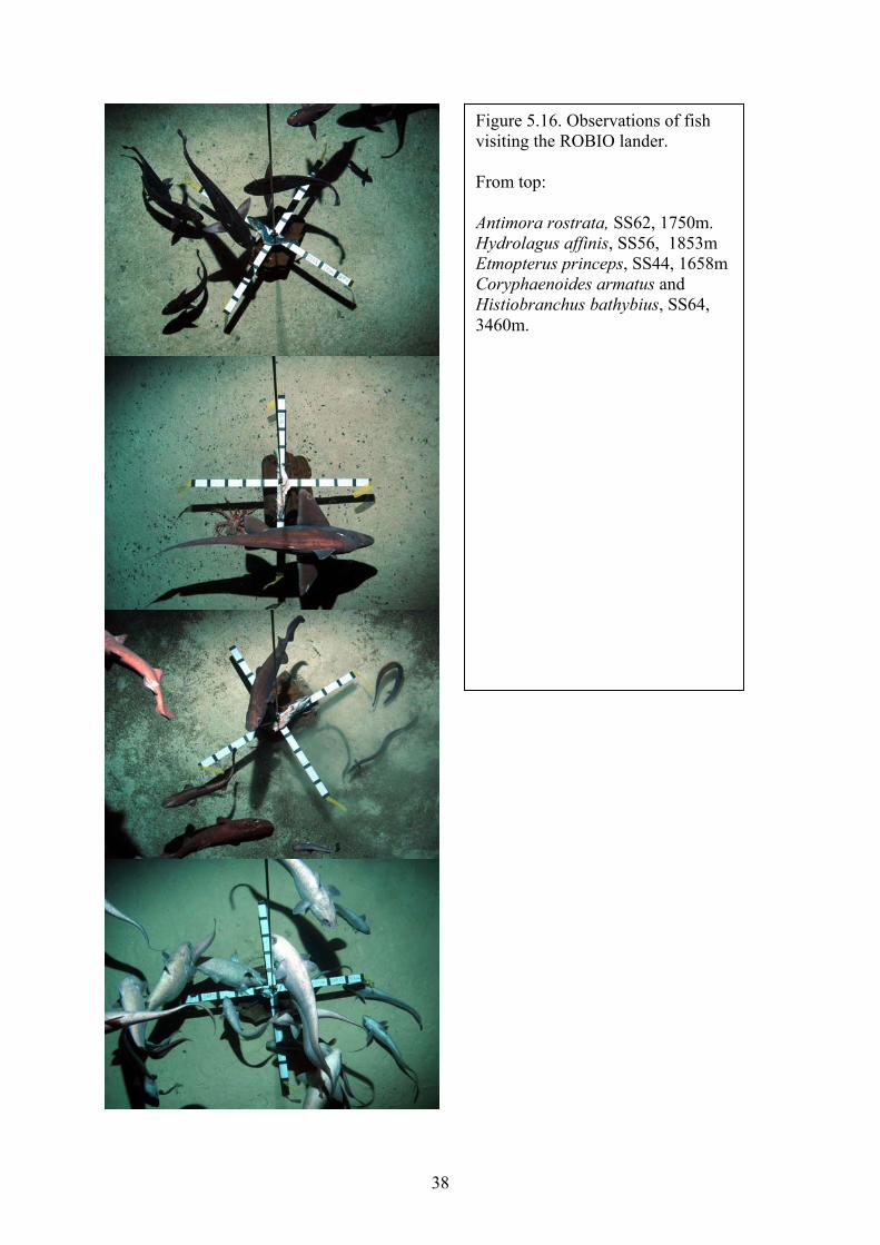
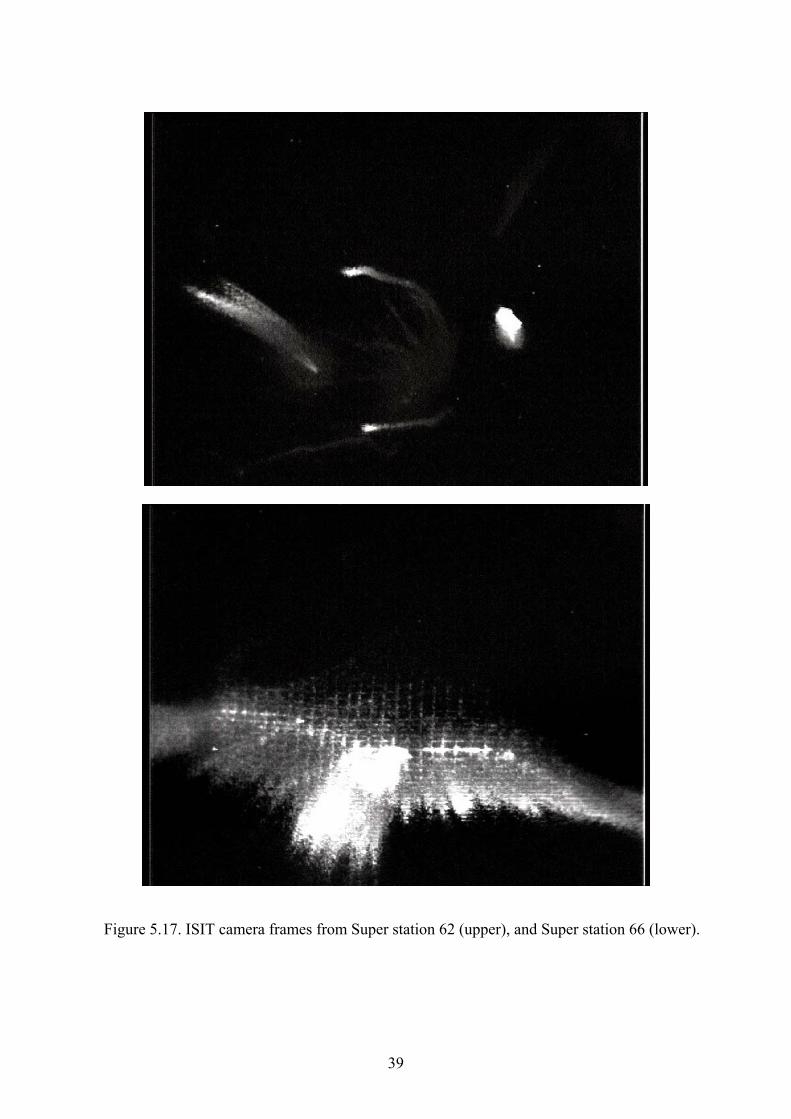
centre of the camera field of view. On descent through the water column the mesh screen stimulates bioluminescent events, which are recorded in monochrome on a 60-minute mini DV tape. The CTD was lowered at a rate of 0.8ms-1. Deployments: The ISIT camera was deployed at 14 stations (SS52-SS76, including SS53) at depths down to 3500m, capturing 14 hours of bioluminescence profiles. Single deployments were conducted in the Southern box (SS52), and one on the Faraday Seamount (SS53). Preliminary results: Initial results indicate a reduction of bioluminescent events with increasing depth at all stations. Some organisms are discernable and there is potential to classify to order level. In some profiles patchiness of events is evident intermittently throughout the profile. Examples of frames from ISIT deployments are shown in Figure 5.17. Analysis: Analysis of ISIT profiles will consist of image analysis; time series counts of bioluminescent events and shape and size classification of events. Analysis will commence in early 2005. 3) Subpopulation dynamics of the armed grenadier, Coryphaenoides armatus: sample collection Samples of white muscle and liver tissue were collected from a total of 133 individuals of C.armatus at 13 superstations (SS40, 42, 50, 52, 54, 56, 62, 64, 66, 68, 70, 72 & 74). Microsatellite and RNA analysis to determine the existence of sub-populations of C.armatus will be conducted in early 2005. 4) Periodic bait release in the Charlie-Gibbs fracture zone: Deep Ocean Benthic Observatory (DOBO) Technology: The Deep Ocean Benthic Observer (DOBO) is an autonomous lander vehicle designed to undergo long duration experiments at depth. Its titanium frame bears a battery unit, controller unit, 35mm stills camera (model M8S, Ocean Instrumentation, UK) and two strobe flash bulbs (200J each) slaved to the camera and illuminating a bait at the base of the lander. Two Kodak E200 Ektachrome colour reversal films spliced together enable a maximum of 1400 images to be taken per deployment. Photographs are taken in a pre-determined sequence. The DOBO bait consists of six mackerel carcasses sealed in individual plastic tubes. Bait tubes are tethered to an autosampler mechanism (KUM) programmed to release at 5-day intervals. This results in an identical bait presentation of one mackerel carcass every five days.

38

Figure 5.16. Observations of fish visiting the ROBIO lander. From top: Antimora rostrata, SS62, 1750m. Hydrolagus affinis, SS56, 1853m Etmopterus princeps, SS44, 1658mCoryphaenoides armatus and Histiobranchus bathybius, SS64, 3460m.

39

Figure 5.17. ISIT camera frames from Super station 62 (upper), and Super station 66 (lower).

40

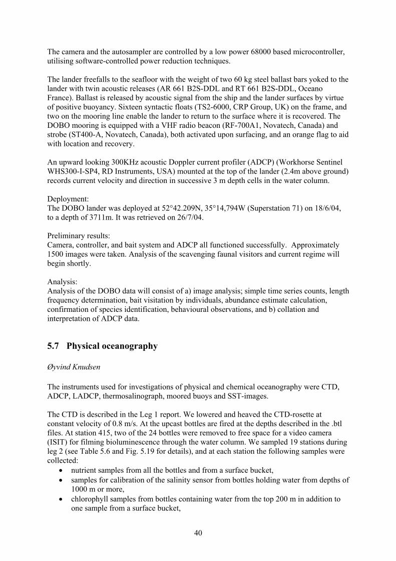
The camera and the autosampler are controlled by a low power 68000 based microcontroller, utilising software-controlled power reduction techniques. The lander freefalls to the seafloor with the weight of two 60 kg steel ballast bars yoked to the lander with twin acoustic releases (AR 661 B2S-DDL and RT 661 B2S-DDL, Oceano France). Ballast is released by acoustic signal from the ship and the lander surfaces by virtue of positive buoyancy. Sixteen syntactic floats (TS2-6000, CRP Group, UK) on the frame, and two on the mooring line enable the lander to return to the surface where it is recovered. The DOBO mooring is equipped with a VHF radio beacon (RF-700A1, Novatech, Canada) and strobe (ST400-A, Novatech, Canada), both activated upon surfacing, and an orange flag to aid with location and recovery. An upward looking 300KHz acoustic Doppler current profiler (ADCP) (Workhorse Sentinel WHS300-I-SP4, RD Instruments, USA) mounted at the top of the lander (2.4m above ground) records current velocity and direction in successive 3 m depth cells in the water column. Deployment: The DOBO lander was deployed at 52°42.209N, 35°14,794W (Superstation 71) on 18/6/04, to a depth of 3711m. It was retrieved on 26/7/04. Preliminary results: Camera, controller, and bait system and ADCP all functioned successfully. Approximately 1500 images were taken. Analysis of the scavenging faunal visitors and current regime will begin shortly. Analysis: Analysis of the DOBO data will consist of a) image analysis; simple time series counts, length frequency determination, bait visitation by individuals, abundance estimate calculation, confirmation of species identification, behavioural observations, and b) collation and interpretation of ADCP data.

5.7 Physical oceanography Øyvind Knudsen The instruments used for investigations of physical and chemical oceanography were CTD, ADCP, LADCP, thermosalinograph, moored buoys and SST-images. The CTD is described in the Leg 1 report. We lowered and heaved the CTD-rosette at constant velocity of 0.8 m/s. At the upcast bottles are fired at the depths described in the .btl files. At station 415, two of the 24 bottles were removed to free space for a video camera (ISIT) for filming bioluminescence through the water column. We sampled 19 stations during leg 2 (see Table 5.6 and Fig. 5.19 for details), and at each station the following samples were collected:

• nutrient samples from all the bottles and from a surface bucket, • samples for calibration of the salinity sensor from bottles holding water from depths of

1000 m or more, • chlorophyll samples from bottles containing water from the top 200 m in addition to

one sample from a surface bucket,

41

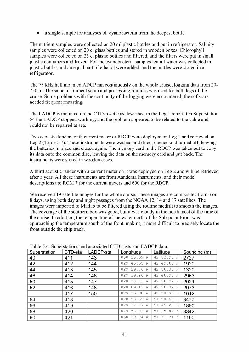
• a single sample for analyses of cyanobacteria from the deepest bottle. The nutrient samples were collected on 20 ml plastic bottles and put in refrigerator. Salinity samples were collected on 20 cl glass bottles and stored in wooden boxes. Chlorophyll samples were collected on 25 cl plastic bottles and filtered, and the filters were put in small plastic containers and frozen. For the cyanobacteria samples ten ml water was collected in plastic bottles and an equal part of ethanol were added, and the bottles were stored in a refrigerator. The 75 kHz hull mounted ADCP ran continuously on the whole cruise, logging data from 20-750 m. The same instrument setup and processing routines was used for both legs of the cruise. Some problems with the continuity of the logging were encountered; the software needed frequent restarting. The LADCP is mounted on the CTD-rosette as described in the Leg 1 report. On Superstation 54 the LADCP stopped working, and the problem appeared to be related to the cable and could not be repaired at sea. Two acoustic landers with current meter or RDCP were deployed on Leg 1 and retrieved on Leg 2 (Table 5.7). These instruments were washed and dried, opened and turned off, leaving the batteries in place and closed again. The memory card in the RDCP was taken out to copy its data onto the common disc, leaving the data on the memory card and put back. The instruments were stored in wooden cases. A third acoustic lander with a current meter on it was deployed on Leg 2 and will be retrieved after a year. All these instruments are from Aanderaa Instruments, and their model descriptions are RCM 7 for the current meters and 600 for the RDCP. We received 19 satellite images for the whole cruise. These images are composites from 3 or 8 days, using both day and night passages from the NOAA 12, 14 and 17 satellites. The images were imported to Matlab to be filtered using the routine medfilt to smooth the images. The coverage of the southern box was good, but it was cloudy in the north most of the time of the cruise. In addition, the temperature of the water north of the Sub-polar Front was approaching the temperature south of the front, making it more difficult to precisely locate the front outside the ship track. Table 5.6. Superstations and associated CTD casts and LADCP data. Superstation CTD-sta LADCP-sta Longitude Latitude Sounding (m) 40 411 143 030 23.69 W 42 52.98 N 2727 42 412 144 029 45.65 W 42 49.65 N 1920 44 413 145 029 29.76 W 42 56.38 N 1320 46 414 146 029 19.26 W 42 46.90 N 2963 50 415 147 028 30.81 W 42 56.92 N 2021 52 416 148 028 09.13 W 42 56.02 N 2973 417 150 029 36.90 W 49 50.99 N 1012 54 418 028 53.52 W 51 20.56 N 3477 56 419 029 32.07 W 51 45.29 N 1890 58 420 029 58.01 W 51 25.42 N 3342 60 421 030 19.04 W 51 31.71 N 1100

42

62 422 030 23.72 W 51 53.79 N 1697 64 423 030 59.62 W 51 32.58 N 3462 66 424 033 33.47 W 53 02.55 N 3067 68 425 034 44.80 W 53 07.43 N 2144 70 426 034 54.94 W 53 00.26 N 1748 72 427 035 30.58 W 53 18.15 N 2435 74 428 036 46.04 W 53 17.55 N 3059 76 429 035 28.18 W 53 05.96 N 1243 Table 5.7. Current meter moorings. Acoustic lander

Longitude Latitude Instrument deployed retrieved Echo-depth

1 029 06.90 W 42 51.99 N RCM 7 28/6 10/7 899 2 035°27.89 W 53°05.98 N RDCP 600 17/6 27/7 1100 3 030°19.83 W 51°31.59 N RCM 7 22/7 868

4e+003

3e+003

3e+003

4e+003

2e+003

3e+003

4e+003

4e+003

3e+003

2e+003

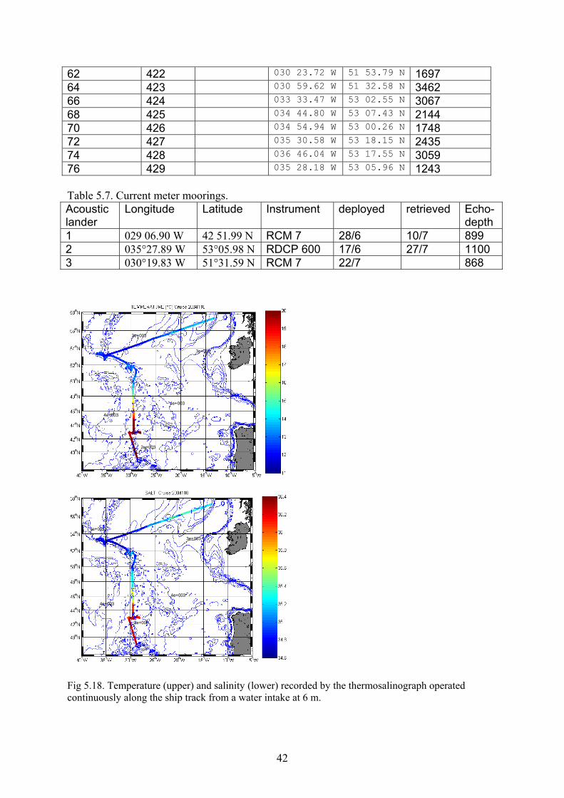
Fig 5.18. Temperature (upper) and salinity (lower) recorded by the thermosalinograph operated continuously along the ship track from a water intake at 6 m.

43

Main results The thermosalinograph showed Atlantic Water (AW) in the surface layer of the Iceland Basin east of about 26°W (Fig. 5.18). West of this and north of 52°N we found a colder Arctic water mass with a salinity of about 34.7 – 34.9 overlying a layer of Subpolar Mode Water (SPMW) from about 200-600 m for the CTD-stations north of the CGFZ, except the westernmost. The surface mixed layer in this area was about 20 – 30 m, and the water column was characterized by low salinities. On the southern side of the CGFZ there was an eddy containing AW in the top 500 m (stations 419-422), surrounded by waters of lower salinity. From about 800-1500 m there was a layer of Labrador Sea Water (LSW) and below that a layer of North Atlantic Deep Water in the middle box. The temperature gradient across the Subpolar Front decreased from Leg 1 to Leg 2, and the front moved 2°-2.5° south to about 49.5°N. The heating of the surface layer was about 3-4°C around CGFZ, decreasing to 1-2°C heating (on shorter time) farther south. In the southern box the differences between Leg 1 and Leg 2 were rather small in the CTD-profiles.

38oW 36oW 34oW 32oW 30oW 28oW 48oN

50oN

52oN

54oN

416

417

418

419

420421

422

423

424425426

427428429

-4500

-4000

-3500

-3000

-2500

30oW 28oW 42oN

44oN

0

411 412413

414

415 416

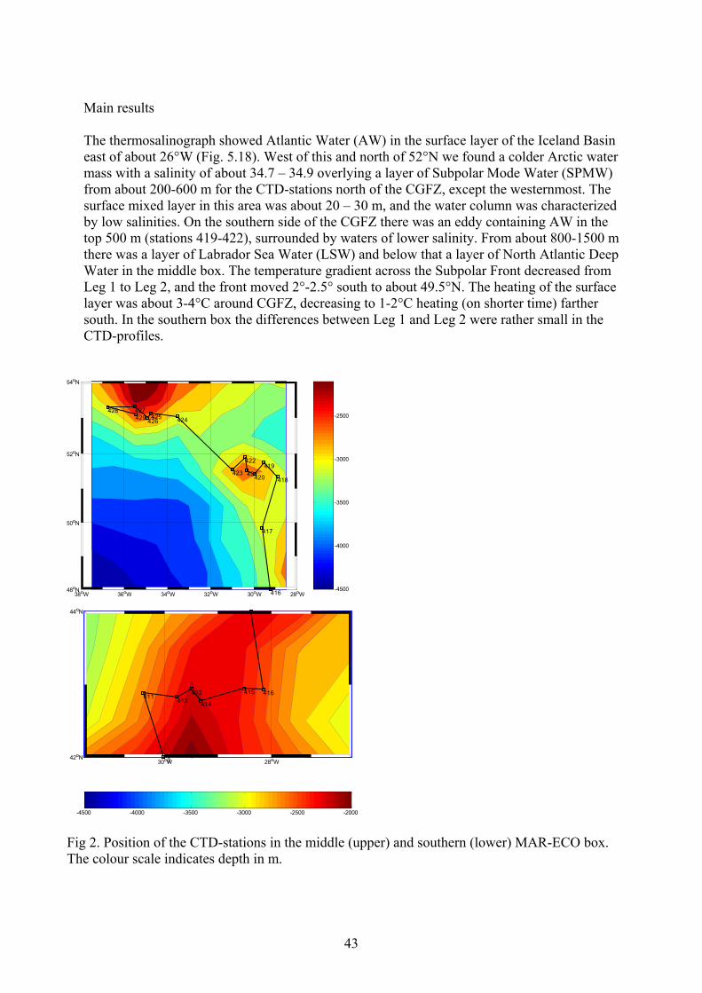
-4500 -4000 -3500 -3000 -2500 -2000 Fig 2. Position of the CTD-stations in the middle (upper) and southern (lower) MAR-ECO box. The colour scale indicates depth in m.