Embed Size (px)
Citation preview

1
Kleene Algebra Modulo Theories
RYAN BECKETT, Princeton UniversityERIC CAMPBELL, Pomona CollegeMICHAEL GREENBERG, Pomona College
Kleene algebras with tests (KATs) o�er sound, complete, and decidable equational reasoning about regularlystructured programs. Since NetKAT demonstrated how well various extensions of KATs apply to computernetworks, interest in KATs has increased greatly. Unfortunately, extending a KAT to a particular domain byadding custom primitives, proving its equational theory sound and complete, and coming up with e�cientautomata-theoretic implementations is still an expert’s task.
We present a general framework for deriving KATs we call Kleene algebra modulo theories: given primitivesand notions of state, we can automatically derive a corresponding KAT’s semantics, prove its equational theorysound and complete, and generate an automata-based implementation of equivalence checking. Our frameworkis based on pushback, a way of specifying how predicates and actions interact, �rst used in Temporal NetKAT.We o�er several case studies, including theories for bitvectors, increasing natural numbers, unbounded setsand maps, temporal logic, and network protocols. Finally, we provide an OCaml implementation that closelymatches the theory: with only a few declarations, users can automatically derive an automata-theoreticdecision procedure for a KAT.
1 INTRODUCTIONKleene algebras with tests (KATs) provide a powerful framework for reasoning about regularlystructured programs. Able to model abstractions of programs with while loops, KATs can handlea variety of analysis tasks [3, 7, 11–13, 34] and typically enjoy sound, complete, and decidableequational theories. Interest in KATs has increased recently as they have been applied to thedomain of computer networks. NetKAT, a language for programming and verifying SoftwareDe�ned Networks (SDNs), was the �rst [1], followed by many variations and extensions [5, 8, 22,35, 37, 46]. However, extending a KAT remains a challenging task, requiring experts familiar withKATs and their metatheory to craft custom domain primitives, derive a collection of new domain-speci�c axioms, prove the soundness and completeness of the resulting algebra, and implement adecision procedure. Our goal in this paper is to democratize KATs, o�ering a general frameworkfor automatically deriving sound, complete, and decidable KATs for client theories. Our theoreticalframework corresponds closely to an OCaml implementation, which derives a KAT with a decisionprocedure from small modules specifying theories.
What is a KAT?. From a bird’s-eye view, a Kleene algebra with tests is a �rst-order languagewith loops (the Kleene algebra) and interesting decision making (the tests). More formally, a KATconsists of two parts: a Kleene algebra 〈0, 1,+, ·, ∗〉 of “actions” with an embedded Boolean algebra〈0, 1,+, ·,¬〉 of “predicates”. KATs are useful for representing propositional programs with whileloops: we use · as sequential composition, + as branching (a/k/a parallel composition), and ∗ foriteration. For example, if α and β are predicates and π and ρ are actions, then the KAT termα · π + ¬α(β · ρ)∗ · ¬β · π de�nes a program denoting two kinds of traces: either α holds and wesimply run π , or α doesn’t hold, and we run ρ until β no longer holds and then run π . Translatingthe KAT term into a While program, we write: if α then π else { while β do { ρ } ; π }.Reasoning in KAT is purely propositional, and the actions and tests are opaque. We know nothingabout α , β , π , or ρ, or how they might interact. For example, π might be the assignment i := i + 1and ρ might be the test i > 100. Clearly these ought to be related—the action π can a�ect the
, Vol. 1, No. 1, Article 1. Publication date: July 2017.
arX
iv:1
707.
0289
4v3
[cs
.PL
] 1
2 Ju
l 201
7

1:2 Ryan Becke�, Eric Campbell, and Michael Greenberg
truth of ρ. To allow for reasoning with respect to a particular domain (e.g., the domain of naturalnumbers with addition and comparison), one typically must extend KAT with additional axiomsthat capture the domain-speci�c behavior [1, 5, 8, 29, 33].
As an example, NetKAT showed how packet forwarding in computer networks can be modeledas simple While programs. Devices in a network must drop or permit packets (tests), update packetsby modifying their �elds (actions), and iteratively pass packets to and from other devices (loops).NetKAT extends KAT with two actions and one predicate: an action to write to packet �elds, f ← v ,where we write valuev to �eld f of the current packet; an action dup, which records a packet in thehistory; and a �eld matching predicate, f = v , which determines whether the �eld f of the currentpacket is set to the value v . Each NetKAT program is denoted as a function from a packet historyto a set of packet histories. For example, the program dstIP← 192.168.0.1 · dstPort← 4747 · duptakes a packet history as input, updates the topmost packet to have a new destination IP addressand port, and then saves the current packet state. The NetKAT paper goes on to explicitly restatethe KAT equational theory along with custom equations for the new primitive forms, prove thetheory’s soundness, and then devise a novel normal form to reduce NetKAT to an existing KATwith a known completeness result. Later papers [21, 50] then developed the NetKAT automatatheory used to compile of NetKAT programs into forwarding tables and to verify existing networks.
We aim to make it easier to de�ne new KATs. Our theoretical framework and its correspondingimplementation allow for quick and easy derivation of sound and complete KATs with automata-theoretic decision procedures when given arbitrary domain-speci�c theories.
How do we build our KATs? Our framework for deriving Kleene algebras with tests requires, ata minimum, custom predicates and actions along with a description of how these apply to somenotion of state. We call these parts the client theory, and we call the client theory’s predicates andactions “primitive”, as opposed to those built with the KAT’s composition operators. We call theresulting KAT a Kleene algebra modulo theory (KMT). Deriving a trace-based semantics for theKMT and proving it sound isn’t particularly hard—it amounts to “turning the crank”. Proving theKMT is complete and decidable, however, can be much harder.
Our framework hinges on an operation relating predicates and operations called pushback, �rstused to prove relative completeness for Temporal NetKAT [8]. Given a primitive action π and aprimitive predicate α , the pushback operation tells us how to go from π · α to some set of terms:∑n
i=0 αi · π = α0 · π + α1 · π + . . . . That is, the client theory must be able to take any of its primitivetests and “push it back” through any of its primitive actions. Pushback allows us to take an arbitraryterm and normalize into a form where all of the predicates appear only at the front of the term, aconvenient representation both for our completeness proof (Section 3.4) and our automata-theoreticimplementation (Sections 5 and 6).
The quid pro quo. Our method takes a client theory T of custom primitive predicates and actions;from the client theory we generate a KMT, T ∗, on top of T . Depending on what we know about T ,we can prove a variety of properties of T ∗; in dependency order:
(1) As a baseline, we need a notion of state and a way to assign meaning to primitive operations;we can then de�ne a semantics for T ∗ that denotes each term as a function from a trace ofstates to a set of traces of states and a log of actions (Section 3.1).
(2) Our resulting semantics is sound as a KAT, with sound client equations added to accountfor primitives (Section 3.2; Theorem 3.5).
(3) If the client theory can de�ne an appropriate pushback operation, we can de�ne a normal-ization procedure for T ∗ (Section 3.3).
, Vol. 1, No. 1, Article 1. Publication date: July 2017.

Kleene Algebra Modulo Theories 1:3
(4) IfT is deductively complete, can decide satis�ability of predicates, and satis�es the pushbackrequirements, then the equational theory for T ∗ is complete and decidable given thetrace-based interpretation of actions (Section 3.4; Theorem 3.40), and we can derive bothan automata-theoretic model of T ∗, and an implementation in OCaml that can decideequivalence of terms in T ∗ (Sections 5 and 6).
What are our contributions?• A new framework for de�ning KATs and proving their metatheory, with a novel, explicit
development of the normalization procedure used in completeness (Section 3).• Several case studies of this framework (Section 4), including a strengthening of Temporal
NetKAT’s completeness result, theories for unbounded state (naturals, sets, and maps), anddistributed routing protocols.• An automata theoretic account of our proof technique, which can inform compilation strategies
for, e.g., NetKAT and enable equivalence checking (Section 5).• An implementation of our framework (Section 6) which follows the proofs directly, automati-
cally deriving automata-theoretic decision procedures for client theories.Finally, our framework o�ers a new way in to those looking to work with KATs. Researchersfamiliar with inductive relations from, e.g., type theory and semantics, will �nd a familiar friend inour generalization of the pushback operation—we de�ne it as an inductive relation.
2 MOTIVATION AND INTUITIONBefore getting into the technical details, we o�er an overview of how KATs are used (Section 2.1),what kinds of KMTs we can de�ne (Section 2.2), and an extended networking example (Section 2.3).
2.1 Modeling While programsHistorically, KAT has been used to model the behavior of simple While programs. The Kleenestar operator (p∗) captures the iterative behavior of while loops, and tests model conditionals inif statements and loop guards. For example, consider the program Pnat (Figure 1a), a short loopover two natural-valued variables. To model such a program in KAT, one replaces each concretetest or action with an abstract representation. Let the atomic test α represent the test i < 50, βrepresent i < 100, and γ represent j > 100; the atomic actions p and q represent the assignmentsi := i + 1 and j := j + 2, respectively. We can now write the program as the KAT expressionα · (β · p · q)∗ · ¬β · γ . The complete equational theory of KAT makes it possible to reason aboutprogram transformations and decide equivalence between KAT terms. For example, KAT’s theorycan prove that the original loop is equivalent to its unfolding, i.e.:
α · (β · p · q)∗ · ¬β · γ ≡ α · (1 + β · p · q) · (β · p · q · β · p · q)∗ · ¬β · γUnfortunately, KATs are naïvely propositional: the algebra understands nothing of the underlyingdomain or the semantics of the abstract predicates and actions. For example, the fact that (j :=j + 2 · j > 200) ≡ (j > 198 · j := j + 2) does not follow from the KAT axioms—to reason using thisequivalence, we must add it as an equational assumption. Reasoning about the particular values ofthe variable i over time in Pnat demands some number of relevant equational assumptions.
While purely abstract reasoning with KAT can often work for particular programs, it requiresthat we know exactly which equational assumptions we need on a per-program basis. Yet the abilityto reason about the equivalence of programs in the presence of particular domains (such as thedomain of natural numbers with addition and comparison) is important in order to model many realprograms and domain-speci�c languages. Can we come up with theories that allow us to reasonin a general way, and not per-program? Yes: we can build our own KAT, adding domain-speci�c
, Vol. 1, No. 1, Article 1. Publication date: July 2017.

1:4 Ryan Becke�, Eric Campbell, and Michael Greenberg
assume i < 50while (i < 100) do
i := i + 1j := j + 2
endassert j > 100
assume 0 ≤ j < 4while (i < 10) doi := i + 1j := (j << 1) + 3if i < 5 theninsert(X, j)
endassert in(X, 9)
i := 0parity := false
while (true) doodd[i] := parity
i := i + 1parity := !parity
endassert odd[99]
(a) Pnat (b) Pset (c) Pmap
Fig. 1. Example simple while programs.
equational rules for our actions. Such an approach is taken by NetKAT [1], which adds the “packetaxioms” for reasoning about packets as they move through the network. Since NetKAT’s equationaltheory has these packet axioms baked in, there’s no need for per-program reasoning. But NetKAT’sgenerality comes at the cost of proving its metatheory and developing an implementation—a highbarrier to entry for those hoping to adapt KAT to their needs.
Our framework for Kleene algebras modulo theories (KMTs) allow us to derive metatheory andimplementation for KATs based on a given theory. KMTs o�er the best of both worlds: obviating bothper-program reasoning and the need to deeply understand KAT metatheory and implementation.
2.2 Building new theoriesWe o�er some cartoons of KMTs here; see Section 4 for technical details.
We can model the program Pnat (Figure 1a) by introducing a new client theory with actionsx := n and x := x + 1 and a new test x > n for some collection of variables x and natural numberconstants n. For this theory we can add axioms like the following (where x , y):
(x := n) · (x > m) ≡ (n > m) · (x := n)(x := x + 1) · (y > n) ≡ (y > n) · (x := x + 1)(x := x + 1) · (x > n) ≡ (x > n − 1) · (x := x + 1)
To derive completeness and decidability for the resulting KAT, the client must know how to takeone of their primitive actions π (here, either x := n or x := x + 1) and any primitive predicate α(here, just x > n) and take π · α and push the test back, yielding an equivalent term b · π , such thatπ · α ≡ b · π and b is in some sense no larger than α . The client’s pushback operation is a criticalcomponent of our metatheory. Here, the last axiom shows how to push back a comparison testthrough an increment action and generate predicates that do not grow in size: x > n−1 is a “smaller”test than x > n. Given, say, a Presburger arithmetic decision procedure, we can automatically verifyproperties, like the assertion j > 100 that appears in Pnat, for programs with while loops.
Consider Pset (Figure 1b), a program de�ned over both naturals and a set data structure with twooperations: insertion and membership tests. The insertion action insert(x , j) inserts the value ofan expression (j) into a given set (x ); the membership test in(x , c) determines whether a constant(c) is included in a given set (x ). An axiom characterizing pushback for this theory has the form:
insert(x , e) · in(x , c) ≡ (e = c) · insert(x , e)Our theory of sets works for expressions e taken from another theory, so long as the underlyingtheory supports tests of the form e = c . For example, this would work over the theory of naturalssince a test like j = 10 can be encoded as (j > 9) · ¬(j > 10).
, Vol. 1, No. 1, Article 1. Publication date: July 2017.

Kleene Algebra Modulo Theories 1:5
Finally, Pmap (Figure 1c) uses a combination of mutable boolean values and a map data structure.Just as before, we can craft custom theories for reasoning about each of these types of state. Forbooleans, we can add actions of the form b := true and b := false and tests of the form b = trueand b = false. The axioms are then simple equivalences like (b := true · b = false) ≡ 0 and(b := true · b = true) ≡ (b := true). To model map data structures, we add actions of the formX[e] := e and tests of the form X[c] = c . Just as with the set theory, the map theory is parameterizedover other theories, which can provide the type of keys and values—here, integers and booleans. InPmap, the odd map tracks whether certain natural numbers are odd or not by storing a boolean intothe map’s index. A sound axiom characterizing pushback in the theory of maps has the form:
(X[e1] := e2 · X[c1] = c2) ≡ (e1 = c1 · e2 = c2 + ¬(e1 = c1) · X[c1] = c2) · X[e1] := e2
Each of the theories we have described so far—naturals, sets, booleans, and maps—have teststhat only examine the current state of the program. However, we need not restrict ourselves inthis way. Primitive tests can make dynamic decisions or assertions based on any previous state ofthe program. As an example, consider the theory of past-time, �nite-trace linear temporal logic(LTLf ) [15, 16]. Linear temporal logic introduces new operators such as: ©a (in the last state a), ♦a(in some previous state a), and �a (in every state a); we use �nite-time LTL because �nite tracesare a reasonable model in most domains modeling programs. As a use of LTLf , we may want tocheck for Pnat (Figure 1a) that, before the last state, the variable j was always less than or equal to200. We can capture this with the test ©�(j ≤ 200). For LTLf , our axioms include equalities likep · ©a ≡ a · p and �a ≡ a · ©�a. We can use these axioms to push tests back through actions; forexample, we can rewrite terms using these LTLf axioms alongside the natural number axioms:
j := j + 2 ·�(j ≤ 200) ≡ j := j + 2 · (j ≤ 200 · ©�(j ≤ 200))≡ (j := j + 2 · j ≤ 200) · ©�(j ≤ 200)≡ (j ≤ 198) · j := j + 2 · ©�(j ≤ 200)≡ (j ≤ 198) ·�(j ≤ 200) · j := j + 2
Pushing the temporal test back through the action reveals that j is never greater than 200 if beforethe action j was not greater than 198 in the previous state and j never exceeded 200 before theaction as well. The �nal pushed back test (j ≤ 198) ·�(j ≤ 200) satis�es the theory requirementsfor pushback not yielding larger tests, since the resulting test is only in terms of the original testand its subterms. Note that we’ve embedded our theory of naturals into LTLf : we can generate acomplete equational theory for LTLf over any other complete theory.
The ability to use temporal logic in KAT means that we can model check programs by phrasingmodel checking questions in terms of program equivalence. For example, for some program r , wecan check if r ≡ r · ©�(j ≤ 200). In other words, if there exists some program trace that does notsatisfy the test, then it will be �ltered—resulting in non-equivalent terms. If the terms are equal,then every trace from r satis�es the test. Similarly, we can test whether r · ©�(j ≤ 200) is empty—ifso, there are no satisfying traces.
Finally, we can encode NetKAT, a system that extends KAT with actions of the form f ← v , wheresome value v is assigned to one of a �nite number of �elds f , and tests of the form f = v where�eld f is tested for value v . It also includes a number of axioms such as f ← v · f = v ≡ f ← v .The NetKAT axioms can be captured in our framework with minor changes. Further extendingNetKAT to Temporal NetKAT is captured trivially in our framework as an application of the LTLftheory to NetKAT’s theory, deriving Beckett et al.’s [8] completeness result compositionally (infact, we can strengthen it—see Section 4.6).
, Vol. 1, No. 1, Article 1. Publication date: July 2017.

1:6 Ryan Becke�, Eric Campbell, and Michael Greenberg
A := 0B :=∞C :=∞D :=∞while (true) doB := min+(A, C, D)C := min+(A, B, D)D := min+(B, C)
end
A := (0, true)B := (0, false)C := (0, false)D := (0, false)while (true) do
updateB
updateC
updateD
end
(a) Sample network with policy on C (b) PSP, default policy (c) PBGP, local policiesFig. 2. An example network and models of BGP routing.
2.3 A case study: network routing protocolsAs a �nal example demonstrating the kinds of theories supported by KMT, we turn our attentionto modeling network routing protocols. While NetKAT uses Kleene algebra to de�ne simple,stateless forwarding tables of networks, the most common network routing protocols are distributedalgorithms that actually compute paths in a network by passing messages between devices. Asan example the Border Gateway Protocol (BGP) [43], which allows users to de�ne rich routingpolicy, has become the de facto internet routing protocol used to transport data between betweenautonomous networks under the control of di�erent entities (e.g. Verizon, Comcast). However, thecombination of the distributed nature of BGP, the di�culty of writing policy per-device, and thefact that network devices can and often do fail [27] all contribute to the fact that network outagescaused by BGP miscon�guration are common [2, 28, 30, 36, 39, 48, 52]. By encoding BGP policiesin our framework, it immediately follows that we can decide properties about networks runningBGP such as “will router A always be able to reach router B after at most 1 link failure".
Figure 2a shows an example network that is con�gured to run BGP. In BGP, devices exchangemessages between neighbors to determine routes to a destination. In the �gure, routerA is connectedto an end host (the line going to the left) and wants to tell other routers how to get to this destination.
In the default behavior of the BGP protocol, each router selects the shortest path among allof its neighbors and then informs each of its neighbors about this route (with the path lengthincreased by one). In e�ect, the devices will compute the shortest paths through the network ina distributed fashion. We can model shortest paths routing in a KMT using the theory of naturalnumbers: in PSP (Figure 2b), each router maintains a distance to the destination. Since A knowsabout the destination, it will start with a distance of 0, while all other routers start with distance∞.Then, iteratively, each other router updates its distance to be 1 more than the minimum of eachof its peers, which is captured by the min+ operator. The behavior of min+ can be described bypushback equivalences like:
B := min+(A,C,D) · B < 3 ≡ (A < 2 +C < 2 + D < 2) · B := min+(A,C,D)BGP gets interesting when users go beyond shortest path routing and also de�ne router-local
policy. In our example network, router C is con�gured with local policy (Figure 2a): router C willblock messages received from D and will prioritize paths received from neighbor B over those fromA (using distance as a tie breaker). In order to accommodate this richer routing behavior, we mustextend our model to PBGP (Figure 2c). Now, each router is associated with a variable storing a tupleof both the distance and whether or not the router has a path to the destination; we write C1 for
, Vol. 1, No. 1, Article 1. Publication date: July 2017.

Kleene Algebra Modulo Theories 1:7
Predicates T ∗preda,b ::= 0 additive identity
| 1 multiplicative identity| ¬a negation| a + b disjunction| a · b conjunction| α primitive predicates (Tα )
Actionsp,q ::= a embedded predicates
| p + q parallel composition| p · q sequential composition| p∗ Kleene star| π primitive actions (Tπ )
Fig. 3. Generalized KAT syntax (client parts highlighted)
the “does C have a path” boolean and C0 for the length of that path, if it exists. We can then createa separate update action for each device in the network to re�ect the semantics of the device’s localpolicy (updateC, etc.). Further, suppose we have a boolean variable failX ,Y for each link betweenrouters X and Y indicating whether or not the link is failed. The update action for router C’s localpolicy can be captured with the following type of equivalence:
updateC ·C0 < 3 ≡ (¬failA,C · (¬B1 + failB,C ) · A1 · (A0 < 2) + ¬failB,C · B1 · (B0 < 2)) · updateC
In order for router C to have a path length < 3 to the destination after applying the local updatefunction, it must have either been the case that B did not have a route to the destination (or theB-C link is down) and A had a route with length < 2 and the A-C link is not down, or B had aroute with length < 2 and the B-C link is not down. Similarly, we would need an axiom to capturewhen router C will have a path to the destination based on equivalences like: updateC · C1 ≡(A1 · ¬failA,C + B1 · ¬failB,C ) · updateC—C has a path to the destination if any of its neighborshas a path to the destination and the corresponding link is not failed.
It is now possible to ask questions such as “if there is any single network link failure, will C everhave a path with length greater than 2?”. Assuming the network program is encoded as ρ, we cananswer this question by checking language non-emptiness for
(failA,C · ¬failB,C + ¬failA,C · failB,C ) · ρ · (C0 > 2) ≡ 0
While we have in a sense come back to a per-program world—PBGP requires de�nitions and axiomsfor each router’s local policy—we can reason in a very complex domain.
3 LIFTING PUSHBACK TO SOUNDNESS AND COMPLETENESSThis section details the structure of our framework for de�ning a KAT in terms of a client the-ory. While we have striven to make this section accessible to readers without much familiaritywith KATs, those completely new to KATs may do well to skip directly to our case studies (Sec-tion 4). Throughout this paper, we mark those parts which must be provided by the client byhighlighting them in marmalade.
We derive a KAT T ∗ (Figure 3) on top of a client theory T where T has two fundamentalparts—predicates α ∈ Tα and actions π ∈ Tπ . We refer to the Boolean algebra over the client theoryas T ∗pred ⊆ T
∗.We can provide results for T ∗ in a pay-as-you-go fashion: given a model for the predicates and
actions of T , we derive a trace semantics for T ∗ (Section 3.1); if T has a sound equational theorywith respect to our semantics, so does T ∗ (Section 3.2); if T has a complete equational theory withrespect to our semantics, so does T ∗ (Section 3.4); and �nally, with just a few lines of code aboutthe structure of T , we can provide an automata-theoretic implementation of T ∗ (Section 5).
, Vol. 1, No. 1, Article 1. Publication date: July 2017.
1:8 Ryan Becke�, Eric Campbell, and Michael Greenberg
The key to our general, parameterized proof is a novel pushback operation (Section 3.3.2): givenan understanding of how to push primitive predicates back to the front of a term, we can derive amethod for �nding normal forms for our completeness proof (Section 3.4).
3.1 SemanticsThe �rst step in turning the client theory T into a KAT is to de�ne a semantics (Figure 4). We cangive any KAT a trace semantics: the meaning of a term is a trace t , which is a non-empty list of logentries l . Each log entry records a state σ and (in all but the initial state) an action π . The clientassigns meaning to predicates and actions by de�ning a set of states State and two functions: oneto determine whether a predicate holds (pred) and another to determine an action’s e�ects (act). Torun a T ∗ term on a state σ , we start with an initial state 〈σ ,⊥〉; when we’re done, we’ll have a setof traces of the form 〈σ0,⊥〉, 〈σ1,π1〉, . . . ,, where σi = act(πi ,σi−1) for i > 0. (A similar semanticsshows up in Kozen’s application of KAT to static analysis [32].)
A reader new to KATs should compare this de�nition with that of NetKAT or Temporal NetKAT [1,8]: de�ned recursively over the syntax, the denotation function collapses predicates and actionsinto a single semantics, using Kleisli composition (written •) to give meaning to sequence and anin�nite union and exponentiation (written −n ) to give meaning to Kleene star. We’ve generalizedthe way that predicates and actions work, though, deferring to two functions that must be de�nedby the client theory: pred and act.
The client’s pred function takes a primitive predicate α and a trace, returning true or false.Predicates can examine the entire trace—no such predicates exist in NetKAT, but those in TemporalNetKAT do. When the pred function returns true, we return the singleton set holding our input trace;when pred returns false, we return the empty set. (Composite predicates follow this same pattern,always returning either a singleton set holding their input trace or the empty set(Lemma 3.4).) It’sacceptable for the pred function to recursively call the denotational semantics, though we haveskipped the formal detail here. Such a feature is particularly useful for de�ning primitive predicatesthat draw from, e.g., temporal logic (see Section 4.8).
The client’s act function takes a primitive action π and the last state in the trace, returning a newstate. Whatever new state comes out is recorded in the trace, along with the action just performed.
3.2 SoundnessProving soundness is relatively straightforward: we only depend on the client’s act and predfunctions, and none of our KAT axioms (Figure 4) even mention the client’s primitives. We do needto use several KAT theorems in our completeness proof (Figure 4, Consequences), the most complexbeing star expansion (Star-Expand), which we take from Temporal NetKAT [8]. We believe thepushback negation theorem (Pushback-Neg) is novel.
Lemma 3.1 (Pushback negation). If p · a ≡ b · p then p · ¬a ≡ ¬b · p.
, Vol. 1, No. 1, Article 1. Publication date: July 2017.

Kleene Algebra Modulo Theories 1:9
Trace de�nitions
σ ∈ Statel ∈ Log ::= 〈σ ,⊥〉 | 〈σ ,π 〉t ∈ Trace = Log+
pred : Tα × Trace→ {true, false}act : Tπ × State→ State
Trace semantics
[[−]] : T ∗ → Trace→ P(Trace)[[0]](t) = ∅[[1]](t) = {t}[[α]](t) = {t | pred(α , t) = true}[[¬a]](t) = {t | [[a]](t) = ∅}[[π ]](t) = {t 〈σ ′,π 〉 | σ ′ = act(π , last(t))}
[[p + q]](t) = [[p]](t) ∪ [[q]](t)[[p · q]](t) = ([[p]] • [[q]])(t)[[p∗]](t) = ⋃
0≤i [[p]]i (t)
(f • д)(t) = ⋃t ′∈f (t ) д(t ′)
f 0(t) = {t}f i+1(t) = (f • f i )(t)
last(. . . 〈σ , _〉) = σ
Kleene Algebrap + (q + r ) ≡ (p + q) + r KA-Plus-Assoc
p + q ≡ q + p KA-Plus-Commp + 0 ≡ p KA-Plus-Zerop + p ≡ p KA-Plus-Idem
p · (q · r ) ≡ (p · q) · r KA-Seq-Assoc1 · p ≡ p KA-Seq-Onep · 1 ≡ p KA-One-Seq
p · (q + r ) ≡ p · q + p · r KA-Dist-L(p + q) · r ≡ p · r + q · r KA-Dist-R
0 · p ≡ 0 KA-Zero-Seqp · 0 ≡ 0 KA-Seq-Zero
1 + p · p∗ ≡ p∗ KA-Unroll-L1 + p∗ · p ≡ p∗ KA-Unroll-R
q + p · r ≤ r → p∗ · q ≤ r KA-LFP-Lp + q · r ≤ q → p · r ∗ ≤ q KA-LFP-R
p ≤ q ⇔ p + q ≡ q
Boolean Algebraa + (b · c) ≡ (a + b) · (a + c) BA-Plus-Dist
a + 1 ≡ 1 BA-Plus-Onea + ¬a ≡ 1 BA-Excl-Mida · b ≡ b · a BA-Seq-Comma · ¬a ≡ 0 BA-Contraa · a ≡ a BA-Seq-Idem
Consequencesp · a ≡ b · p →
p · ¬a ≡ ¬b · p Pushback-Negp · (q · p)∗ ≡ (p · q)∗ · p Sliding(p + q)∗ ≡ q∗ · (p · q∗)∗ Denesting
p · a ≡ a · q + r →p∗ · a ≡ (a + p∗ · r ) · q∗ Star-Inv
p · a ≡ a · q + r →p · a · (p · a)∗ ≡(a · q + r ) · (q + r )∗ Star-Expand
Fig. 4. Semantics and equational theory for T ∗
Proof. We show that both sides p · ¬a and ¬b · p are equivalent to ¬b · p · ¬a by way ofBA-Excl-Mid:
p · ¬a ≡ (b + ¬b) · p · ¬a (KA-Seq-One, BA-Excl-Mid)≡ b · p · ¬a + ¬b · p · ¬a (KA-Dist-L)≡ p · a · ¬a + ¬b · p · ¬a (assumption)≡ p · 0 + ¬b · p · ¬a (BA-Contra)≡ ¬b · p · ¬a (KA-Plus-Comm, KA-Plus-Zero)≡ 0 · p + ¬b · p · ¬a (BA-Contra)≡ ¬b · b · p + ¬b · p · ¬a (assumption)≡ ¬b · p · a + ¬b · p · ¬a (KA-Dist-R)≡ ¬b · p · (a + ¬a) (KA-One-Seq, BA-Excl-Mid)≡ ¬b · p
, Vol. 1, No. 1, Article 1. Publication date: July 2017.

1:10 Ryan Becke�, Eric Campbell, and Michael Greenberg
�
Our soundness proof naturally enough requires that any equations the client theory adds needto be sound in our trace semantics.
Lemma 3.2 (Kleisli composition is associative). [[p]] • ([[q]] • [[r ]]) = ([[p]] • [[q]]) • [[r ]].
Proof. We compute:[[p · (q · r )]](t) = ⋃
t ′∈[[p]](t )[[q · r ]](t ′)=
⋃t ′∈[[p]](t )
⋃t ′′∈[[q]](t ′)[[r ]](t ′′)
=⋃
t ′′∈⋃t ′∈[[p]](t )[[q]](t ′)[[r ]](t′′)
=⋃
t ′′∈[[p ·q]](t )[[r ]](t ′′)= [[(p · q) · r ]](t)
�
Lemma 3.3 (Exponentiation commutes). [[p]]i+1 = [[p]]i • [[p]]
Proof. By induction on i . When i = 0, both yield [[p]]. In the inductive case, we compute:[[p]]i+2 = [[p]] • [[p]]i+1
= [[p]] • ([[p]]i • [[p]]) by the IH= ([[p]] • [[p]]i ) • [[p]] by Lemma 3.2= ([[p]]i+1) • [[p]] by Lemma 3.2
�
Lemma 3.4 (Predicates produce singleton or empty sets). [[a]](t) ⊆ {t}.
Proof. By induction on a, leaving t general.(a = 0) We have [[a]](t) = ∅.(a = 1) We have [[a]](t) = {t}.(a = α ) If pred(α , t) = true, then our output trace is {t}; otherwise, it is ∅.(a = ¬b) We have [[¬a]](t) = {t | [[b]](t) = ∅}. By the IH, [[b]](t) is either ∅ (in which case we get{t} as our output) or {t} (in which case we get ∅).
(a = b + c) By the IHs.(a = b · c) We get [[b · c]](t) = ⋃
t ′ in[[b]](t )[[c]](t ′). By the IH on b, we know that b yields eitherthe set {t} or the emptyset; by the IH on c , we �nd the same.
�
Theorem 3.5 (Soundness of T ∗). If T ’s equational reasoning is sound (p ≡T q ⇒ [[p]] = [[q]])then T ∗’s equational reasoning is sound (p ≡ q ⇒ [[p]] = [[q]]).
Proof. By induction on the derivation of p ≡ q.1
(KA-Plus-Assoc) We have p + (q + r ) ≡ (p + q) + r ; by associativity of union.(KA-Plus-Comm) We have p + q ≡ q + p; by commutativity of union.(KA-Plus-Zero) We have p + 0 ≡ p; immediate, since [[0]](t) = ∅.(KA-Plus-Idem) By idempotence of union p + p ≡ p.(KA-Seq-Assoc) We have p · (q · r ) ≡ (p · q) · r ; by Lemma 3.2.(KA-Seq-One) We have 1 · p ≡ p; immediate, since [[1]](t) = {t}.(KA-One-Seq) We have p · 1 ≡ p; immediate, since [[1]](t) = {t}.
1Full proofs with all necessary lemmas are available in an extended version of this paper in the supplementary material.
, Vol. 1, No. 1, Article 1. Publication date: July 2017.

Kleene Algebra Modulo Theories 1:11
(KA-Dist-L) We have p · (q + r ) ≡ p · q + p · r ; we compute:
[[p · (q + r )]](t) = ⋃t ′∈[[p]](t )[[q + r ]](t ′)
=⋃
t ′∈[[p]](t )[[q]](t ′) ∪ [[r ]](t ′)=
⋃t ′∈[[p]](t )[[q]](t ′) ∪
⋃t ′∈[[p]](t )[[r ]](t ′)
= [[p · q]](t) ∪ [[p · r ]](t)= [[p · q + p · r ]](t)
(KA-Dist-R) We have (p + q) · r ≡ p · r + q · r ; we compute:
[[(p + q) · r ]](t) = ⋃t ′∈[[p+q]](t )[[r ]](t ′)
=⋃
t ′∈[[p]](t )∪[[q]](t )[[r ]](t ′)=
⋃t ′∈[[p]](t )[[r ]](t ′) ∪
⋃t ′∈[[q]](t )[[r ]](t ′)
= [[p · r ]](t) ∪ [[q · r ]](t)= [[p · r + q · r ]](t)
(KA-Zero-Seq) We have 0 · pequiv0; immediate, since [[0]](t) = ∅.(KA-Seq-Zero) We have p · 0equiv0; immediate, since [[0]](t) = ∅.(KA-Unroll-L) We have p∗ ≡ 1 + p · p∗. We compute:
[[p∗]](t) = ⋃0≤i [[p]]i (t)
= [[1]](t) ∪⋃1≤i [[p]]i (t)
= [[1]](t) ∪ [[p]](t) ∪⋃2≤i [[p]]i (t))
= [[1]](t) ∪ ([[p]] • [[1]])(t) ∪⋃1≤i ([[p]] • [[p]]i )(t)
= [[1]](t) ∪ ([[p]] • [[1]])(t ′) ∪ ([[p]] •⋃1≤i [[p]]i )(t)= [[1]](t) ∪ ([[p]] •⋃0≤i [[p]]i )(t)= [[1]](t) ∪ [[p · p∗]](t))= [[1 + p · p∗]](t)
(KA-Unroll-R) We have p∗ ≡ 1+p∗ ·p. We compute, using Lemma 3.3 to unroll the exponentialin the other direction:
[[p∗]](t) = ⋃0≤i [[p]]i (t)
= [[1]](t) ∪⋃1≤i [[p]]i (t)
= [[1]](t) ∪ [[p]](t) ∪⋃2≤i [[p]]i (t)
= [[1]](t) ∪ [[p]](t) ∪⋃1≤i ([[p]]i • [[p]])(t ′) by Lemma 3.3
= [[1]](t) ∪ ([[1]] • [[p]])(t) ∪⋃1≤i ([[p]]i • [[p]])(t ′)
= [[1]](t) ∪⋃0≤i ([[p]]i • [[p]])(t ′)
= [[1]](t) ∪ (⋃0≤i [[p]]i • [[p]])(t ′)= [[1]](t) ∪ [[p∗ · p]](t)= [[1 + p∗ · p]](t)
(KA-LFP-L) We have p∗ · q ≤ r , i.e., p∗ · q + r ≡ r . By the IH, we know that [[q]](t) ∪ ([[p]] •[[r ]])(t) ∪ [[r ]](t) = [[r ]](t). We show, by induction on i , that ([[p]]i • [[q]])(t) ∪ [[r ]](t) = [[r ]](t).
(i = 0) We compute:
([[p]]0 • [[q]])(t) ∪ [[r ]](t)= ([[1]] • [[q]])(t) ∪ [[r ]](t)= [[q]](t) ∪ [[r ]](t)= [[q]](t) ∪ ([[q]](t) ∪ ([[p]] • [[r ]])(t) ∪ [[r ]]) by the outer IH= [[q]](t) ∪ ([[p]] · [[r ]])(t) ∪ [[r ]](t)= [[r ]](t) by the outer IH again
, Vol. 1, No. 1, Article 1. Publication date: July 2017.
1:12 Ryan Becke�, Eric Campbell, and Michael Greenberg
(i = i ′ + 1) We compute:([[p]]i′+1 • [[q]])(t) ∪ [[r ]](t)= ([[p]] • [[p]]i′ • [[q]])(t) ∪ [[r ]](t)= ([[p]] • [[p]]i′ • [[q]])(t) ∪ ([[q]](t) ∪ ([[p]] • [[r ]])(t) ∪ [[r ]](t)) by the outer IH=
⋃t ′∈[[p]](t )(
⋃t ′′∈[[p]]i′ (t ′)[[q]](t ′) ∪ [[r ]](t ′)) ∪ ([[q]](t) ∪ [[r ]](t))
= ([[p]] • [[r ]])(t) ∪ ([[q]](t) ∪ [[r ]](t)) by the inner IH= [[r ]](t) by the outer IH again
So, �nally, we have:
[[p∗ · q + r ]](t) = (⋃0≤i[[p]]i • [[q]])(t) ∪ [[r ]](t) =
⋃0≤i([[p]]i • [[q]])(t) ∪ [[r ]](t)) =
⋃0≤i[[r ]](t) = [[r ]](t)
(KA-LFP-R) We have p · r ∗ ≤ q, i.e., p · r ∗ + q ≡ q. By the IH, we know that [[p]](t) ∪ ([[q]] •[[r ]])(t) ∪ [[q]](t) = [[q]](t). We show, by induction on i , that ([[p]] • [[r ]]i )(t) ∪ [[q]](t) = [[q]](t).
(i = 0) We compute:([[p]] • [[r ]]0)(t) ∪ [[q]](t)= ([[p]] • [[1]])(t) ∪ [[q]](t)= [[p]](t) ∪ [[q]](t)= [[p]](t) ∪ [[p]](t) ∪ ([[q]] • [[r ]])(t) ∪ [[q]](t) by the outer IH= [[p]](t) ∪ ([[q]] • [[r ]])(t) ∪ [[q]](t)= [[q]](t)
(i = i ′ + 1) We compute:([[p]] • [[r ]]i′+1)(t ′) ∪ [[q]](t)= ([[p]] • [[r ]]i′ • [[r ]])(t) ∪ [[q]](t) by Lemma 3.3= ([[p]] • [[r ]]i′ • [[r ]])(t) ∪ [[p]](t) ∪ ([[q]] • [[r ]])(t) ∪ [[q]](t) by the outer IH=
⋃t ′∈[[p]](t )
⋃t ′′∈[[r ]]i′ (t ′)∪[[q]](t )[[r ]](t ′′) ∪ [[p]](t) ∪ [[q]](t)
=⋃
t ′∈⋃t ′′∈[[p]](t )[[r ]]i′ (t ′′)∪[[q]](t )[[r ]](t ′) ∪ [[p]](t) ∪ [[q]](t)
= ([[q]] • [[r ]])(t) ∪ [[p]](t) ∪ [[q]](t) by the inner IH= [[q]](t) by the inner IH again
So, �nally, we have:
[[p · r ∗ + q]](t) = ([[p]] •⋃0≤i[[r ]]i )(t) ∪ [[q]](t) =
⋃0≤i([[p]] • [[r ]]i )(t) ∪ [[q]](t)) =
⋃0≤i[[q]](t) = [[q]](t)
(BA-Plus-Dist) We have a+(b ·c) ≡ (a+b)·(a+c). We have [[a+(b ·c)]](t) = [[a]](t)∪([[b]]•[[c]])(t).By Lemma 3.4, we know that each of these denotations produces either {t} or ∅, where ∪ isdisjunction and • is conjunction. By distributivity of these operations.
(BA-Plus-One) We have a + 1 ≡ 1; we have this directly by Lemma 3.4.(BA-Excl-Mid) We have a + ¬a ≡ 1; we have this directly by Lemma 3.4 and the de�nition of
negation.(BA-Seq-Comm) a · b ≡ b · a; we have this directly by Lemma 3.4 and unfolding the union.(BA-Contra) We have a · ¬a ≡ 0; we have this directly by Lemma 3.4 and the de�nition of
negation.(BA-Seq-Idem) a · a ≡ a; we have this directly by Lemma 3.4 and unfolding the union.
�
For the duration of this section, we assume that any equations T adds are sound and, so, T ∗ issound by Theorem 3.5.
, Vol. 1, No. 1, Article 1. Publication date: July 2017.
Kleene Algebra Modulo Theories 1:13
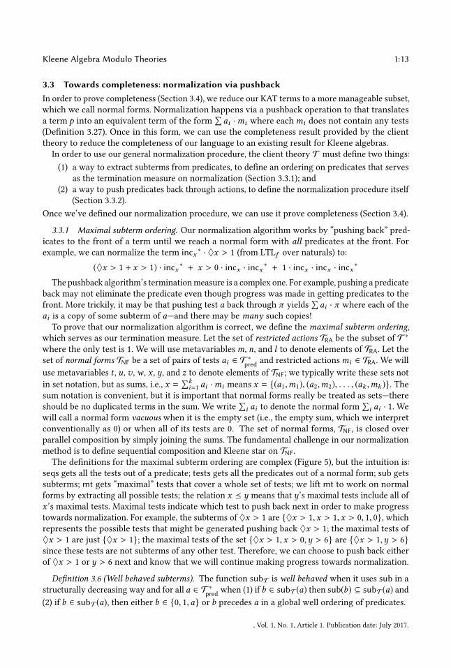
3.3 Towards completeness: normalization via pushbackIn order to prove completeness (Section 3.4), we reduce our KAT terms to a more manageable subset,which we call normal forms. Normalization happens via a pushback operation to that translatesa term p into an equivalent term of the form
∑ai ·mi where eachmi does not contain any tests
(De�nition 3.27). Once in this form, we can use the completeness result provided by the clienttheory to reduce the completeness of our language to an existing result for Kleene algebras.
In order to use our general normalization procedure, the client theory T must de�ne two things:(1) a way to extract subterms from predicates, to de�ne an ordering on predicates that serves
as the termination measure on normalization (Section 3.3.1); and(2) a way to push predicates back through actions, to de�ne the normalization procedure itself
(Section 3.3.2).Once we’ve de�ned our normalization procedure, we can use it prove completeness (Section 3.4).
3.3.1 Maximal subterm ordering. Our normalization algorithm works by “pushing back” pred-icates to the front of a term until we reach a normal form with all predicates at the front. Forexample, we can normalize the term incx ∗ · ♦x > 1 (from LTLf over naturals) to:
(♦x > 1 + x > 1) · incx ∗ + x > 0 · incx · incx ∗ + 1 · incx · incx · incx ∗
The pushback algorithm’s termination measure is a complex one. For example, pushing a predicateback may not eliminate the predicate even though progress was made in getting predicates to thefront. More trickily, it may be that pushing test a back through π yields
∑ai · π where each of the
ai is a copy of some subterm of a—and there may be many such copies!To prove that our normalization algorithm is correct, we de�ne the maximal subterm ordering,
which serves as our termination measure. Let the set of restricted actions TRA be the subset of T ∗where the only test is 1. We will use metavariablesm, n, and l to denote elements of TRA. Let theset of normal forms TNF be a set of pairs of tests ai ∈ T ∗pred and restricted actions mi ∈ TRA. We willuse metavariables t , u, v , w , x , y, and z to denote elements of TNF; we typically write these sets notin set notation, but as sums, i.e., x =
∑ki=1 ai ·mi means x = {(a1,m1), (a2,m2), . . . , (ak ,mk )}. The
sum notation is convenient, but it is important that normal forms really be treated as sets—thereshould be no duplicated terms in the sum. We write
∑i ai to denote the normal form
∑i ai · 1. We
will call a normal form vacuous when it is the empty set (i.e., the empty sum, which we interpretconventionally as 0) or when all of its tests are 0. The set of normal forms, TNF, is closed overparallel composition by simply joining the sums. The fundamental challenge in our normalizationmethod is to de�ne sequential composition and Kleene star on TNF.
The de�nitions for the maximal subterm ordering are complex (Figure 5), but the intuition is:seqs gets all the tests out of a predicate; tests gets all the predicates out of a normal form; sub getssubterms; mt gets “maximal” tests that cover a whole set of tests; we lift mt to work on normalforms by extracting all possible tests; the relation x � y means that y’s maximal tests include all ofx ’s maximal tests. Maximal tests indicate which test to push back next in order to make progresstowards normalization. For example, the subterms of ♦x > 1 are {♦x > 1,x > 1,x > 0, 1, 0}, whichrepresents the possible tests that might be generated pushing back ♦x > 1; the maximal tests of♦x > 1 are just {♦x > 1}; the maximal tests of the set {♦x > 1,x > 0,y > 6} are {♦x > 1,y > 6}since these tests are not subterms of any other test. Therefore, we can choose to push back eitherof ♦x > 1 or y > 6 next and know that we will continue making progress towards normalization.
De�nition 3.6 (Well behaved subterms). The function subT is well behaved when it uses sub in astructurally decreasing way and for all a ∈ T ∗pred when (1) if b ∈ subT(a) then sub(b) ⊆ subT(a) and(2) if b ∈ subT(a), then either b ∈ {0, 1,a} or b precedes a in a global well ordering of predicates.
, Vol. 1, No. 1, Article 1. Publication date: July 2017.

1:14 Ryan Becke�, Eric Campbell, and Michael Greenberg
Sequenced tests and test of normal forms seqs : T ∗pred → P(T∗pred)
seqs : P(T ∗pred) → P(T∗pred) tests : T ∗nf → P(T
∗pred)
seqs(a · b) = seqs(a) ∪ seqs(b)seqs(a) = {a}
seqs(A) = ⋃a∈A seqs(a)
tests(∑ai ·mi ) = {1} ∪ {ai }
Subterms sub : T ∗pred → P(T∗pred) subT : Tα → P(T ∗pred) sub : P(T ∗pred) → P(T
∗pred)
sub(0) = {0}sub(1) = {0, 1}sub(α) = {0, 1,α } ∪ subT(α)
sub(¬a) = {0, 1} ∪ sub(a) ∪ {¬b | b ∈ sub(a)}sub(a + b) = {a + b} ∪ sub(a) ∪ sub(b)sub(a · b) = {a · b} ∪ sub(a) ∪ sub(b)
sub(A) =⋃a∈A
sub(a)
Maximal tests mt : P(T ∗pred) → P(T∗pred) mt : T ∗nf → P(T
∗pred)
mt(A) = {b ∈ seqs(A) | ∀c ∈ seqs(A), c , b ⇒ b < sub(c)} mt(x) = mt(tests(x))
Maximal subterm ordering �,≺,≈ ⊆ T ∗nf × T∗nf
x � y ⇐⇒ sub(mt(x)) ⊆ sub(mt(y)) x ≺ y ⇐⇒ sub(mt(x)) ( sub(mt(y))x ≈ y ⇐⇒ x � y ∧ y � x
Fig. 5. Maximal tests and the maximal subterm ordering
In most cases, it’s su�cient to use the size of terms as the well ordering, but as we develophigher-order theories, we use a lexicographic ordering of “universe level” paired with term size.Throughout the following, we assume that subT is well behaved.
Lemma 3.7 (Terms are subterms of themselves). a ∈ sub(a)
Proof. By induction on a. All cases are immediate except for ¬a, which uses the IH. �
Lemma 3.8 (0 is a subterm of all terms). 0 ∈ sub(a)
Proof. By induction on a. The cases for 0, 1, and α are immediate; the rest of the cases followby the IH. �
Lemma 3.9 (Maximal tests are tests). mt(A) ⊆ seqs(A) for all sets of tests A.
Proof. We have by de�nition:
mt(A) = {b ∈ seqs(A) | ∀c ∈ seqs(A), c , b ⇒ b < sub(c)}⊆ seqs(A)
�
Lemma 3.10 (Maximal tests contain all tests). seqs(A) ⊆ sub(mt(A)) for all sets of tests A.
, Vol. 1, No. 1, Article 1. Publication date: July 2017.

Kleene Algebra Modulo Theories 1:15
Proof. Let an a ∈ seqs(A) be given; we must show that a ∈ sub(mt(A)). If a ∈ mt(A), thena ∈ sub(mt(A)) (Lemma 3.7). If a < mt(A), then there must exist a b ∈ mt(A) such that a ∈ sub(b).But in that case, a ∈ sub(b) ∪⋃
a∈mt(A)\{b } sub(mt(a)), so a ∈ sub(mt(A)). �
Lemma 3.11 (seqs distributes over union). seqs(A ∪ B) = seqs(A) ∪ seqs(B)
Proof. We compute:
seqs(A ∪ B) = ⋃c ∈A∪B seqs(c)
=⋃
c ∈A seqs(c) ∪⋃c ∈B seqs(C)
= seqs(A) ∪ seqs(B)�
Lemma 3.12 (seqs is idempotent). seqs(a) = seqs(seqs(a))
Proof. By induction on a.(a = b · c) We compute:
seqs(seqs(b · c)) = seqs(seqs(b) ∪ seqs(c))= seqs(seqs(b)) ∪ seqs(seqs(c)) (by the IH)= seqs(b) ∪ seqs(c)= seqs(b · c)
(a = 0, 1,α ,¬b,b + c) We compute:
seqs(a) = {a}= seqs(a)=
⋃a∈{a } seqs(a)
= seqs({a})= seqs(seqs(a))
�
NB that we can lift Lemma 3.12 to sets of terms, as well.
Lemma 3.13 (Seqence extraction). If seqs(a) = {a1, . . . ,ak } then a ≡ a1 · · · · · ak .
Proof.(a = b · c) We have:
{a1, . . . ,ak } = seqs(a) = seqs(b · c) = seqs(b) ∪ seqs(c).
Furthermore, seqs(b) (resp. seqs(c)) is equal to some subset of the ai ∈ seqs(a), such that seqs(b) ∪seqs(c) = seqs(a). By the IH, we know that b ≡ Πbi ∈seqs(b)bi and c ≡ Πci ∈seqs(c)ci , so we have:
a ≡ b · c≡
(∏bi ∈seqs(b) bi
)·(∏
bi ∈seqs(b) bi)
(BA-Seq-Idem)≡ ∏
ai ∈seqs(b)∪seqs(c) ai (BA-Seq-Comm)≡ ∏k
i=1 ai
(a = 0, 1,α ,¬b,b + c) Immediate by re�exivity, since seqs(a) = {a}. �
Corollary 3.14 (Maximal tests are invariant over tests). mt(A) = mt(seqs(A))
, Vol. 1, No. 1, Article 1. Publication date: July 2017.

1:16 Ryan Becke�, Eric Campbell, and Michael Greenberg
Proof. We compute:mt(A) = {b ∈ seqs(A) | ∀c ∈ seqs(A), c , b ⇒ b < sub(c)}
(Lemma 3.12)= {b ∈ seqs(seqs(A)) | ∀c ∈ seqs(seqs(A)), c , b ⇒ b < sub(c)}= mt(seqs(A))
�
Lemma 3.15 (Subterms are closed under subterms). If a ∈ sub(b) then sub(a) ⊆ sub(b).
Proof. By induction on b, letting some a ∈ sub(b) be given.(b = 0) We have sub(0) = {0}, so it must be that a = 0 and sub(a) = sub(b).(b = 1) We have sub(0) = {0, 1}; either a = 0 (and so sub(a) = {0} ⊆ sub(1)) or a = 1 (and so
sub(a) = sub(b)).(b = α ) Immediate, since subT is well behaved.(b = ¬c) a is either in sub(c) or a = ¬d and d ∈ sub(c). We can use the IH either way.(b = c + d) We have sub(b) = {c + d} ∪ sub(c) ∪ subd . If a is in the �rst set, we have a = b and
we’re done immediately. If a is in the second set, we have sub(a) ⊆ sub(c) by the IH, and sub(c) isclearly a subset of sub(b). If a is in the third set, we similarly have sub(a) ⊆ sub(d) ⊆ sub(b).
(b = c · d) We have sub(b) = {c · d} ∪ sub(c) ∪ subd . If a is in the �rst set, we have a = b andwe’re done immediately. If a is in the second set, we have sub(a) ⊆ sub(c) by the IH, and sub(c) isclearly a subset of sub(b). If a is in the third set, we similarly have sub(a) ⊆ sub(d) ⊆ sub(b).
�
Lemma 3.16 (Subterms decrease in size). If a ∈ sub(b), then either a ∈ {0, 1,b} or a comesbefore b in the global well ordering.
Proof. By induction on b.(b = 0) Immediate, since sub(b) = {0}.(b = 1) Immediate, since sub(b) = {0, 1}.(b = α ) By the assumption that subT(α) is well behaved.(b = ¬c) Either a = ¬c—and we’re done immediately, or a , ¬c , so a is a possibly negated
subterm of c . In the latter case, we’re done by the IH.(b = c + d) Either a = c+d—and we’re done immediately, or a , c+d , and so a ∈ sub(c)∪sub(d).
In the latter case, we’re done by the IH.(b = c · d) Either a = c · d—and we’re done immediately, or a , c · d , and so a ∈ sub(c) ∪ sub(d).
In the latter case, we’re done by the IH.�
Lemma 3.17 (Maximal tests always exist). If A is a non-empty set of tests, then mt(A) , 0.
Proof. We must show there exists at least one term in mt(A).If seqs(A) = {a}, then a is a maximal test. If seqs(A) = {0, 1}, then 1 is a maximal test. If
seqs(A) = {0, 1,α }, then α is a maximal test. If seqs(A) isn’t any of those, then let aseqsA be theterm that comes last in the well ordering on predicates.
To see why a ∈mt(A), suppose (for a contradiction) we haveb ∈ mt(A) suchb , a and a ∈ sub(b).By Lemma 3.16, either a ∈ {0, 1,b} or a comes before b in the global well ordering. We’ve ruledout the �rst two cases above. If a = b, then we’re �ne—a is a maximal test. But if a comes before bin the well ordering, we’ve reached a contradiction, since we selected a as the term which comeslatest in the well ordering. �
, Vol. 1, No. 1, Article 1. Publication date: July 2017.

Kleene Algebra Modulo Theories 1:17
As a corollary, note that a maximal test exists even for vacuous normal forms, where mt(x) = {0}when x is vacuous.
Lemma 3.18 (Maximal tests generate subterms). sub(mt(A)) = ⋃a∈seqs(A) sub(a)
Proof. Since mt(A) ⊆ seqs(A) (Lemma 3.9), we can restate our goal as:
sub(mt(A)) =⋃
a∈mt(A)sub(a) ∪
⋃a∈seqs(A)\mt(A)
sub(a)
We have sub(mt(A)) = ⋃a∈mt(A) sub(a) by de�nition; it remains to see that the latter union is
subsumed by the former; but we have seqs(A) ⊆ sub(mt(A)) by Lemma 3.10. �
Lemma 3.19 (Union distributes over maximal tests).sub(mt(A ∪ B)) = sub(mt(A)) ∪ sub(mt(B))
Proof. We compute:sub(mt(A ∪ B)) = ⋃
a∈seqs(A∪B) sub(a) (Lemma 3.18)=
⋃a∈seqs(A)∪seqs(B) sub(a)
=[⋃
a∈seqs(A) a]∪
[⋃b ∈seqs(B) sub(b)
]= sub(mt(A)) ∪ sub(mt(B)) (Lemma 3.18)
�
Lemma 3.20 (Maximal tests are monotonic). If A ⊆ B then sub(mt(A)) ⊆ sub(mt(B)).
Proof. We have sub(mt(B)) = sub(mt(A∪B)) = sub(mt(A))∪ sub(mt(B)) (by Lemma 3.19). �
Corollary 3.21 (Seqences of maximal tests). sub(mt(a · b)) = sub(mt(a)) ∪ sub(mt(b))
Proof.sub(mt(c · d))
= sub(mt(seqs(c · d))) (Corollary 3.14)= sub(mt(seqs(c) ∪ seqs(d)))= sub(mt(seqs(c))) ∪ sub(mt(seqs(d))) (distributivity; Lemma 3.19)= sub(mt(c)) ∪ sub(mt(d)) (Corollary 3.14)
�
Lemma 3.22 (Negation normal form is monotonic). If a � b then nnf(¬a) � ¬b.
Proof. By induction on a.(a = 0) We have nnf(¬0) = 1 and 1 � ¬b by de�nition.(a = 1) We have nnf(¬1) = 0 and 0 � ¬b by de�nition.(a = α ) We have nnf(¬α) = ¬α ; since a � b, it must be that α ∈ sub(mt(b)), so ¬α ∈
sub(mt(¬b)). We have α ∈ sub(¬b), since α ∈ sub(b).(a = ¬c) We have nnf(¬¬c) = nnf(c); since c ∈ sub(a) and a � b, it must be that c ∈ sub(mt(b)),
so nnf(c) � ¬b by the IH.(a = c + d) We have nnf(¬(c +d)) = nnf(¬c) ·nnf(¬d); since c and d are subterms of a and a � b,¬c and ¬d must be in sub(mt(¬b)), and we are done by the IHs.
(a = c · d) We have nnf(¬(c ·d)) = nnf(¬c)+ nnf(¬d); since c and d are subterms of a and a � b,¬c and ¬d must be in sub(mt(¬b)), and we are done by the IHs.
�
, Vol. 1, No. 1, Article 1. Publication date: July 2017.

1:18 Ryan Becke�, Eric Campbell, and Michael Greenberg
Lemma 3.23 (Normal form ordering). For all tests a,b, c and normal forms x ,y, z, the followinginequalities hold:
(1) a � a · b (extension);(2) if a ∈ tests(x), then a � x (subsumption);(3) x ≈ ∑
a∈tests(x ) a (equivalence);(4) if x � x ′ and y � y ′, then x + y � x ′ + y ′ (normal-form parallel congruence);(5) if x + y � z, then x � z and y � z (inversion);(6) if a � a′ and b � b ′, then a · b � a′ · b ′ (test sequence congruence);(7) if a � x and b � x then a · b � x (test bounding);(8) if a � b and x � c then a · x � b · c (mixed sequence congruence);(9) if a � b then nnf(¬a) � ¬b (negation normal-form monotonic).
Each of the above equalities also hold replacing � with ≺, excluding the equivalence (3).
Proof. We prove each properly independently and in turn.(1) We must show that a � a · b (extension); we compute:
sub(mt(a)) = sub(mt(seqs(a)) (Corollary 3.14)⊆ sub(mt(seqs(a))) ∪ sub(mt(seqs(b)))= sub(mt(seqs(a) ∪ seqs(b)))
(distributivity; Lemma 3.19)= sub(mt(seqs(a · b)))= sub(mt(a · b)) (Corollary 3.14)
(2) We must show that if a ∈ tests(x), then a � x (subsumption). We have sub(mt({a})) ⊆sub(mt(tests(x))) by monotonicity (Lemma 3.20) immediately.
(3) We must show that x ≈ ∑a∈tests(x ) a (equivalence). Let x =
∑ai · mi , and recall that∑
aintests(x ) a really denotes the normal form∑
a∈tests(x ) a · 1. We compute:
sub(mt(x)) = sub(mt(tests(x)))= sub(mt({ai }))= sub(mt(⋃a∈tests(x ) a))= sub(mt(tests(∑a∈tests(x ) a · 1)))= sub(mt(∑a∈tests(x ) a))
(4) We must show that if x � x ′ and y � y ′, then x + y � x ′ + y ′ (normal-form parallelcongruence). Unfolding de�nitions, we �nd sub(mt(x)) ⊆ sub(mt(x ′)) and sub(mt(y)) ⊆sub(mt(y ′)). We compute:
sub(mt(x + y))= sub(mt(tests(x + y)))= sub(mt(tests(x) ∪ tests(y)))= sub(mt(tests(x))) ∪ sub(mt(tests(y))) (distributivity; Lemma 3.19)⊆ sub(mt(tests(x ′))) ∪ sub(mt(tests(y ′))) (assumptions)= sub(mt(tests(x ′) ∪ tests(y ′))) (distributivity; Lemma 3.19)= sub(mt(x ′ + y ′))
(5) We must show that if x +y � z, then x � z andy � z (inversion). We have sub(mt(x +y)) =sub(mt(x)) ∪ sub(mt(y)) by distributivity (Lemma 3.19). Since we’ve assumed sub(mt(x +y)) ⊆ sub(mt(z)), we must have sub(mt(x)) ⊆ sub(mt(z)) (and similarly for y).
, Vol. 1, No. 1, Article 1. Publication date: July 2017.

Kleene Algebra Modulo Theories 1:19
(6) We must show that if a � a′ and b � b ′, then a · b � a′ · b ′ (test sequence congruence). Un-folding our assumptions, we have sub(mt(a)) ⊆ sub(mt(a′)) and sub(mt(b)) ⊆ sub(mt(b ′)).We can compute:
sub(mt(a · b)) = sub(mt(a)) ∪ sub(mt(b)) (Corollary 3.21)⊆ sub(mt(a′)) ∪ sub(mt(b ′))= sub(mt(a′ · b ′)) (Corollary 3.21)
(7) We must show that if a � x and b � x then a · b � x (test bounding). Immediate byCorollary 3.21.
(8) We must show that if a � b and x � c then a · x � b · c (mixed sequence congruence). Wecompute:
sub(mt(a · x)) = sub(mt(tests(∑a · ai ·mi )))= sub(mt({a} ∪ {ai }))= sub(mt(a)) ∪ sub(mt(x)) (Corollary 3.21)⊆ sub(mt(b)) ∪ sub(mt(c))= sub(mt(b · c)) (Corollary 3.21)
(9) A restatement of Lemma 3.22.�
Lemma 3.24 (Test seqence split). If a ∈ mt(c) then c ≡ a · b for some b ≺ c .
Proof. We have a ∈ seqs(c) by de�nition. Suppose seqs(c) = {a, c1, . . . , ck }. By sequenceextraction, we have c ≡ a · c1 · · · · · ck (Lemma 3.13). So let b = c1 · · · · · ck ; we must show b ≺ c , i.e.,sub(mt(b)) ( sub(mt(c)). Note that {c1, . . . , ck } = seqs(b). We �nd:
sub(mt(b)) ( sub(mt(c))m (Corollary 3.14)
sub(mt(seqs(b))) ( sub(mt(seqs(c)))m
sub(mt({c1, . . . , ck })) ( sub(mt({a, c1, . . . , ck }))m (distributivity; Lemma 3.19)⋃k
i=1 sub(mt({ci })) ( sub(mt(a)) ∪⋃ki=1 sub(mt({ci }))
Since a ∈ mt(c), we know that none of a < sub(mt(ci )). But a know that terms are subterms ofthemselves (Lemma 3.7), so a ∈ sub(a) = sub(mt(a)). �
Lemma 3.25 (Maximal test ineqality). If a ∈ mt(y) and x � y then either a ∈ mt(x) or x ≺ y.
Proof. Since a ∈ mt(y), we have a ∈ sub(mt(y)). Since x � y, we know that sub(mt(x)) ⊆sub(mt(y)). We go by cases on whether or not a ∈ mt(x):
(a ∈ mt(x)) We are done immediately.(a < mt(x)) In this case, we show that a < sub(mt(x)) and therefore x ≺ y. Suppose, for a
contradiction, that a ∈ sub(mt(x)). Since a < mt(x), there must exist some b ∈ sub(mt(x)) wherea ∈ sub(b). But since x � y, we must also have b ∈ sub(mt(y))... and so it couldn’t be that case thata ∈ mt(y)). We can conclude that it must, then, be the case that a < sub(mt(x)) and so x ≺ y.
�
We can take a normal form x and split it around a maximal test a ∈ mt(x) such that we have apair of normal forms: a · y + z, where both y and z are smaller than x in our ordering, because a (1)appears at the front of y and (2) doesn’t appear in z at all.
, Vol. 1, No. 1, Article 1. Publication date: July 2017.

1:20 Ryan Becke�, Eric Campbell, and Michael Greenberg
Lemma 3.26 (Splitting). If a ∈ mt(x), then there exist y and z such that x ≡ a · y + z and y ≺ xand z ≺ x .
Proof. Suppose x =∑k
i=1 ci ·mi . We have a ∈ mt(x), so, in particular:
a ∈ seqs(tests(x)) = seqs(tests(k∑i=1
ci ·mi )) = seqs({c1, . . . , ck }) =k⋃i=1
seqs(ci ).
That is, a ∈ seqs(ci ) for at least one i . We can, without loss of generality, rearrange x into two sums,where the �rst j elements have a in them but the rest don’t, i.e., x ≡ ∑j
i=1 ci ·mi +∑k
i=j+1 ci ·miwhere a ∈ seqs(ci ) for 1 ≤ i ≤ j but a < seqs(ci ) for j + 1 ≤ i ≤ k . By subsumption (Lemma 3.23),we have ci � x . Since a ∈ mt(x), it must be that a ∈ mt(ci ) for 1 ≤ i ≤ j (instantiating Lemma 3.25with the normal form ci · 1). By test sequence splitting (Lemma 3.24), we �nd that ci ≡ a · bi withbi ≺ ci � x for 1 ≤ i ≤ j, as well.
We are �nally ready to producey and z: they are the �rst j tests with a removed and the remainingtests which never had a, respectively. Formally, let y =
∑ji=1 bi ·mi ; we immediately have that
a · y ≡ ∑ji=1 ci ·mi ; let z =
∑ki=j+1 ci ·mi . We can conclude that x ≡ a · y + z.
It remains to be seen that y ≺ x and z ≺ x . The argument is the same for both; presenting itfor y, we have a < seqs(y) (because of sequence splitting), so a < sub(mt(y)). But we assumeda ∈ mt(x), so a ∈ sub(mt(x)), and therefore y ≺ x . The argument for z is nearly identical but needsno recourse to sequence splitting—we never had any a ∈ seqs(ci ) for j + 1 ≤ i ≤ k . �
Splitting is the key lemma for making progress pushing tests back, allowing us to take a normalform and slowly push its maximal tests to the front; its proof follows from a chain of lemmas givenin the supplementary material.
3.3.2 Pushback. In order to de�ne normalization—necessary for completeness (Section 3.4)—theclient theory must have a pushback operation.
De�nition 3.27 (Pushback). Let the sets ΠT = {π ∈ T ∗} and AT = {α ∈ T ∗}. Then the pushbackoperation of the client theory is a relation PB ⊆ ΠT × AT × P(T ∗pred). We write the relation asπ · α PB
∑ai · π and read it as “α pushes back through π to yield
∑ai · π”. We require that if
π · α PB {a1, . . . ,ak }, then π · α ≡ ∑ki=1 ai · π , and ai � a.
Given the client theory’s PB relation, we de�ne a normalization procedure for T ∗ (Figure 6) byextending the client’s PB relation (Figure 7). The PB relation need not be a function, nor do the theai need to be obviously related to α or π in any way.
The top-level normalization routine is de�ned by the p norm x relation (Figure 6), a syntaxdirected relation that takes a term p and produces a normal form x =
∑i aimi . Most syntactic forms
are easy to normalize: predicates are already normal forms (Pred); primitive actions π are normalforms where there’s just one summand and the predicate is 1 (Act); and parallel composition oftwo normal forms means just joining the sums (Par). But sequence and Kleene star are harder: wede�ne judgments using PB to lift these operations to normal forms.
For sequences, we can recursively take p · q and normalize p into x =∑ai · mi and q into
y =∑bj · nj . But how can we combine x and y into a new normal form? We can concatenate and
rearrange the normal forms to get∑
i, j ai ·mi · bj · nj . If we can push bj back throughmi to �ndsome new normal form
∑ck · lk , then
∑i, j,k ai · ck · lk ·nj is a normal form. We use the PBJ relation
(Figure 6), which joins two normal forms along the lines described here; we write x ·y PBJ z to meanthat the concatenation of x and y is equivalent to the normal form z—the · is merely suggestivenotation, as are other operators that appear on the left-hand side of the judgment schemata.
, Vol. 1, No. 1, Article 1. Publication date: July 2017.

Kleene Algebra Modulo Theories 1:21
Normalization p norm x
a norm aPred
π norm 1 · πAct
p norm x q norm y
p + q norm x + yPar
p norm x q norm y x · y PBJ z
p · q norm zSeq
p norm x x∗ PB∗ y
p∗ norm yStar
Sequential composition of normal forms x · y PBJ z
mi · bj PB• xi j(∑i ai ·mi ) · (
∑j bj · nj ) PBJ ∑
i∑
j ai · xi j · njJoin
Normalization of star x∗ PB∗ y
0∗ PB∗ 1StarZero
x ≺ a x · a PBT y y∗ PB∗ y ′ y ′ · x PBJ z
(a · x)∗ PB∗ 1 + a · zSlide
x ⊀ a x · a PBT a · t + u(t + u)∗ PB∗ y y · x PBJ z
(a · x)∗ PB∗ 1 + a · zExpand
a < mt(z) y . 0 y∗ PB∗ y ′
x · y ′ PBJ x ′ (a · x ′)∗ PB∗ z y ′ · z PBJ z ′
(a · x + y)∗ PB∗ z ′Denest
Fig. 6. Normalization T ∗
For Kleene star, we can take p∗ and normalize p into x =∑ai ·mi , but x∗ isn’t a normal form—we
need to somehow move all of the tests to the front. We do so with the PB∗ relation (Figure 6),writing x∗ PB∗ y to mean that the Kleene star of x is equivalent to the normal form y—the ∗ isagain just suggestive notation. The PB∗ relation is more subtle than PBJ. There are four possibleways to treat x , based on how it factors via splitting (Lemma 3.26): if x = 0, then our work is trivialsince 0∗ ≡ 1 (StarZero); if x splits into a · x ′ where a is a maximal test and there are no othersummands, then we can either use the KAT sliding lemma (Lemma 3.30)to pull the test out when ais strictly the largest test in x (Slide) or by using the KAT expansion lemma (Lemma 3.33)otherwise(Expand); if x splits into a · x ′ + z, we use the KAT denesting lemma (Lemma 3.31)to pull a outbefore recurring on what remains (Denest).
The PBJ and PB∗ relations rely on others to do their work (Figure 7): the bulk of the work happensin the PB• relation, which pushes a test back through a restricted action; PBR and PBT are wrappersaround PB• it for pushing tests back through normal forms and for pushing normal forms backthrough restricted actions, respectively. We write m · a PB• y to mean that pushing the test aback through restricted actionm yields the equivalent normal form y. The PB• relation works byanalyzing both the action and the test. The client theory’s PB relation is used in PB• when we tryto push a primitive predicate α through a primitive action π (Prim); all other KAT predicates canbe handled by rules matching on the action or predicate structure, deferring to other PB relations.To handle negation, we de�ne a function nnf that takes a predicate and translates it to negationnormal form, where negations only appear on primitive predicates (Figure 7); the Pushback-Negtheorem justi�es this case(Lemma 3.1); we use nnf to guarantee that we obey the maximal subtermordering.
De�nition 3.28 (Negation normal form). The negation normal form of a term p is a term p ′ suchthat p ≡ p ′ and negations occur only on primitive predicates in p ′.
, Vol. 1, No. 1, Article 1. Publication date: July 2017.

1:22 Ryan Becke�, Eric Campbell, and Michael Greenberg
Lemma 3.29 (Terms are eqivalent to their negation-normal forms). nnf(p) ≡ p andnnf(p) is in negation normal form.
Proof. By induction on the size of p.(p = 0) Immediate.(p = 1) Immediate.(p = α ) Immediate.(p = π ) Immediate.(p = ¬a) By cases on a.(a = 0) We have ¬0 ≡ 1 immediately, and the latter is clearly negation free.(a = 1) We have ¬1 ≡ 0; as above.(a = α ) We have ¬alpha, which is in normal form.(a = b + c) We have ¬(b + c) ≡ ¬b · ¬c as a consequence of BA-Excl-Mid and soundness
(Theorem 3.5). By the IH on ¬b and ¬c , we �nd that nnf(¬b) ≡ ¬b and nnf(¬c) ≡ ¬c—where theleft-hand sides are negation normal. So transitively, we have ¬(b + c) ≡ nnf(¬b) · nnf(¬c), and thelatter is negation normal.
(a = b · c) We have ¬(b · c) ≡ ¬b + ¬c as a consequence of BA-Excl-Mid and soundness(Theorem 3.5). By the IH on ¬b and ¬c , we �nd that nnf(¬b) ≡ ¬b and nnf(¬c) ≡ ¬c—where theleft-hand sides are negation normal. So transitively, we have ¬(b · c) ≡ nnf(¬b) + nnf(¬c), and thelatter is negation normal.
(p = q + r ) By the IHs on q and r .(p = q · r ) By the IHs on q and r .(p = q∗) By the IH on q.
�
To elucidate the way PB• handles structure, suppose we have the term (π1+π2) · (α1+α2). One oftwo rules could apply: we could split up the tests and push them through individually (SeqParTest),or we could split up the actions and push the tests through together (SeqParAction). It doesn’tparticularly matter which we do �rst: the next step will almost certainly be the other rule, and inany case the results will be equivalent from the perspective of our equational theory. It could bethe case that choosing a one rule over another could give us a smaller term, which might yield amore e�cient normalization procedure. Similarly, a given normal form may have more than onemaximal test—and therefore be splittable in more than one way (Lemma 3.26)—and it may be thatdi�erent splits produce more or less e�cient terms. We haven’t yet studied di�ering strategies forpushback, but see Sections 5 and 6 for discussion of our automata-theoretic implementation.
Lemma 3.30 (Sliding). p · (q · p)∗ ≡ (p · q)∗ · p.
Proof. �
Lemma 3.31 (Denesting). (p + q)∗ ≡ q∗ · (p · q∗)∗.
Proof. �
Lemma 3.32 (Star invariant). If p · a ≡ a · q + r then p∗ · a ≡ (a + p∗ · r ) · q∗.
Proof. �
Lemma 3.33 (Star expansion). If p · a ≡ a · q + r then p · a · (p · a)∗ ≡ (a · q + r ) · (q + r )∗.
Proof. �
, Vol. 1, No. 1, Article 1. Publication date: July 2017.
Kleene Algebra Modulo Theories 1:23
Pushback m · a PB• y m · x PBR y x · a PBT y
m · 0 PB• 0SeqZero
m · 1 PB• 1 ·mSeqOne
m · a PB• y y · b PBT z
m · (a · b) PB• zSeqSeqTest
n · a PB• x m · x PBR y
(m · n) · a PB• ySeqSeqAction
m · a PB• x m · b PB• y
m · (a + b) PB• x + ySeqParTest
m · a PB• x n · a PB• y
(m + n) · a PB• x + ySeqParAction
π · α PB {a1, . . . }π · α PB•
∑i ai · π
Primπ · a PB•
∑i ai · π nnf(¬(∑i ai )) = bπ · ¬a PB• b · π
PrimNeg
m · a PB• x x ≺ am∗ · x PBR y
m∗ · a PB• a + ySeqStarSmaller
m · a PB• a · t + u m∗ · t PBR xu∗ PB∗ y x · y PBJ z
m∗ · a PB• a · y + zSeqStarInv
m · ai PB• xim ·∑i ai · ni PBR ∑
i xi · niRestricted
mi · a PB•∑
j bi j ·mi j
(∑i ai ·mi ) · a PBT ∑i∑
j ai · bi j ·mi jTest
Negation normal form nnf : T ∗pred → T∗pred
nnf(0) = 0nnf(1) = 1nnf(α) = α
nnf(a + b) = nnf(a) + nnf(b)nnf(a · b) = nnf(a) · nnf(b)
nnf(¬0) = 1nnf(¬1) = 0nnf(¬α) = ¬α
nnf(¬¬a) = nnf(a)nnf(¬(a + b)) = nnf(¬a) · nnf(¬b)nnf(¬(a · b)) = nnf(¬a) + nnf(¬b)
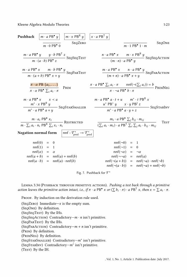
Fig. 7. Pushback for T ∗
Lemma 3.34 (Pushback through primitive actions). Pushing a test back through a primitiveaction leaves the primitive action intact, i.e., if π · a PB• x or (∑bi · π ) · a PBT x , then x =
∑ai · π .
Proof. By induction on the derivation rule used.(SeqZero) Immediate—x is the empty sum.(SeqOne) By de�nition.(SeqSeqTest) By the IHs.(SeqSeqAction) Contradictory—m · n isn’t primitive.(SeqParTest) By the IHs.(SeqParAction) Contradictory—m + n isn’t primitive.(Prim) By de�nition.(PrimNeg) By de�nition.(SeqStarSmaller) Contradictory—m∗ isn’t primitive.(SeqStarInv) Contradictory—m∗ isn’t primitive.(Test) By the IH.
, Vol. 1, No. 1, Article 1. Publication date: July 2017.

1:24 Ryan Becke�, Eric Campbell, and Michael Greenberg
�
We show that our notion of pushback is correct in two steps. First we prove that pushback ispartially correct, i.e., if we can form a derivation in the pushback relations, the right-hand sidesare equivalent to the left-hand-sides (Theorem 3.35). Once we’ve established that our pushbackrelations’ derivations mean what we want, we have to show that we can �nd such derivations;here we use our maximal subterm measure to show that the recursive tangle of our PB relationsalways terminates (Theorem 3.36) , which makes extensive use of our subterm ordering lemma(Lemma 3.23) and splitting (Lemma 3.26)).
Theorem 3.35 (Pushback soundness).
(1) If x · y PBJ z ′ then x · y ≡ z ′.(2) If x∗ PB∗ y then x∗ ≡ y.(3) Ifm · a PB• y thenm · a ≡ y.(4) Ifm · x PBR y thenm · x ≡ y.(5) If x · a PBT y then x · a ≡ y.
Proof. By simultaneous induction on the derivations. Cases are grouped by judgment.
Sequential composition of normal forms (x · y PBJ z).
(Join) We have x =∑k
i=1 ai ·mi and y =∑l
j=1 bj · nj . By the IH on (3), eachmi · bj PB• xi j . Wecompute:
x · y≡
[∑ki=1 ai ·mi
]·[∑l
j=1 bj · nj]
≡ ∑ki=1 ai ·mi ·
[∑lj=1 bj · nj
](KA-Dist-R)
≡ ∑ki=1 ai ·
[mi ·
∑lj=1 bj · nj
](KA-Seq-Assoc)
≡ ∑ki=1 ai ·
[∑lj=1mi · bj · nj
](KA-Dist-L)
≡ ∑ki=1 ai ·
[∑lj=1 xi j · nj
](IH (3))
≡ ∑ki=1
∑lj=1 ai · xi j · nj (KA-Dist-L)
Kleene star of normal forms (x∗ PBJ y).
(StarZero) We have 0∗ PB∗ 1. We compute:
0∗≡ 1 + 0 · 0∗ (KA-Unroll-L)≡ 1 + 0 (KA-Zero-Seq)≡ 1 (KA-Plus-Zero)
(Slide) We are trying to pushback the minimal term a of x through a star, i.e., we have (a · x)∗;by the IH on (5), we know there exists some y such that x · a ≡ y; by the IH on (2), we know thaty∗ ≡ y ′; and by the IH on (1), we know that y ′ · x ≡ z. We must show that (a · x)∗ ≡ 1 + a · z. We
, Vol. 1, No. 1, Article 1. Publication date: July 2017.

Kleene Algebra Modulo Theories 1:25
compute:
(a · x)∗≡ 1 + a · x · (a · x)∗ (KA-Unroll-L)≡ 1 + a · (x · a)∗ · x (sliding with p = x and q = a; Lemma 3.30)≡ 1 + a · y∗ · x (IH (5))≡ 1 + a · y ′ · x (IH (2))≡ 1 + a · z (IH (1))
(Expand) We are trying to pushback the minimal term a of x through a star, i.e., we have (a ·x)∗;by the IH on (5), we know that there exist t and u such that x · a ≡ a · t + u; by the IH on (2), weknow that there exists a y such that (t + u)∗ ≡ y; and by the IH on (1), we know that there is somez such that y · x ≡ z. We compute:
(a · x)∗≡ 1 + a · x + a · x · a · x · (a · x)∗ (KA-Unroll-L)≡ 1 + a · x + a · x · a · (x · a)∗ · x
(sliding with p = x and q = a; Lemma 3.30)≡ 1 + a · x + a · [x · a · (x · a)∗] · x (KA-Seq-Assoc)≡ 1 + a · x + a · [(a · t + u) · (t + u)∗] · x
(expansion using IH (5); Lemma 3.33)≡ 1 + a · x + a · (a · t + u) · (t + u)∗ · x (KA-Seq-Assoc)≡ 1 + a · x + (a · a · t + a · u) · (t + u)∗ · x (KA-Dist-L)≡ 1 + a · x + (a · t + a · u) · (t + u)∗ · x (BA-Seq-Idem)≡ 1 + a · x + a · (t + u) · (t + u)∗ · x (BA-Seq-Idem)≡ 1 + a · 1 · x + a · (t + u) · (t + u)∗ · x (KA-One-Seq)≡ 1 + (a · 1 + a · (t + u) · (t + u)∗) · x (KA-Dist-R)≡ 1 + a · (1 + (t + u) · (t + u)∗) · x (KA-Dist-L)≡ 1 + a · (t + u)∗ · x (KA-Unroll-L)≡ 1 + a · y · x (IH (2))≡ 1 + a · z (IH (1))
(Denest) We have a compound normal form a ·x+y under a star; we will push back the maximaltest a. By our �rst IH on (2) we know that that y∗ ≡ y ′ for some y ′; by our �rst IH on (1), we knowthat x · y ′ ≡ x ′ for some x ′; by our second IH on (2), we know that (a · x ′)∗ ≡ z for some z; and byour second IH on (1), we know that y ′ · z ≡ z ′ for some z ′. We must show that (a · x + y)∗ ≡ z ′. Wecompute:
(a · x + y)∗≡ y∗ · (a · x · y∗)∗ (denesting with p = a · x and q = y; Lemma 3.31)≡ y ′ · (a · x · y ′)∗ (�rst IH (2))≡ y ′ · (a · x ′)∗ (�rst IH (1))≡ y ′ · z (second IH (2))≡ z ′ (second IH (1))
Pushing tests through actions (m · a PB• y).
(SeqZero) We are pushing 0 back through a restricted action m. We immediately �nd m · 0 ≡ 0by KA-Seq-Zero.
, Vol. 1, No. 1, Article 1. Publication date: July 2017.

1:26 Ryan Becke�, Eric Campbell, and Michael Greenberg
(SeqOne) We are pushing 1 back through a restricted actionm. We �nd:m · 1
≡ m (KA-One-Seq)≡ 1 ·m (KA-Seq-One)
(SeqSeqTest) We are pushing the tests a · b through the restricted actionm. By our �rst IH on(3), we havem · a ≡ y; by our second IH on (3), we have y · b ≡ z. We compute:
m · (a · b)≡ m · a · b (KA-Seq-Assoc)≡ y · b (�rst IH (3))≡ z (second IH (3))
(SeqSeqAction) We are pushing the test a through the restricted actionsm · n. By our IH on(3), we have n · a ≡ x ; by our IH on (4), we havem · x ≡ y. We compute:
(m · n) · a≡ m · (n · a) (KA-Seq-Assoc)≡ m · x (IH (3))≡ y (IH (4))
(SeqParTest) We are pushing the tests a + b through the restricted actionm. By our �rst IH on(3), we havem · a ≡ x ; by our second IH on (3), we havem · b ≡ y. We compute:
m · (a + b)m · a +m · b (KA-Dist-L)
≡ x +m · b (�rst IH (3))≡ x + y (second IH (3))
(SeqParAction) We are pushing the test a through the restricted actions m + n. By our �rst IHon (3), we havem · a ≡ x ; by our second IH on (3), we have n · a ≡ y. We compute:
(m + n) · am · a + n · a (KA-Dist-R)
≡ x + n · a (�rst IH (3))≡ x + y (second IH (3))
(Prim) We are pushing a primitive predicate α through a primitive action π . We have, byassumption, that π · a PB {a1, . . . ,ak }. By de�nition of the PB relation, it must be the case thatπ · α ≡ ∑k
i=1 ai · π(PrimNeg) We are pushing a negated predicate ¬a back through a primitive action π . We have,
by assumption, that π · a PB•∑
i ai · pi and that nnf(¬(∑i ai )) = b, so ¬(∑i ai ) ≡ b (Lemma 3.29).By the IH, we know that π · a ≡ ∑
i ai · π ; we must show that π · ¬a ≡ b · π . By our assumptions,we know that b · π ≡ ¬(∑i ai ) · π , so by pushback negation (Pushback-Neg/Lemma 3.1).
(SeqStarSmaller) We are pushing the test a through the restricted actionm∗. By our IH on (3),we havem · a ≡ x for some x ; by our IH on (4), we havem∗ · x ≡ y for some y. We compute:
m∗ · a≡ (1 +m∗ ·m) · a (KA-Unroll-R)≡ a +m∗ ·m · a (KA-Dist-R)≡ a +m∗ · (m · a) (KA-Seq-Assoc)≡ a +m∗ · x (IH (3))≡ a + y (IH (4))
, Vol. 1, No. 1, Article 1. Publication date: July 2017.

Kleene Algebra Modulo Theories 1:27
(SeqStarInv) We are pushing the test a through the restricted actionm∗. By our IH on (3), thereexist t and u such that m · a ≡ a · t + u; by our IH on (4), there exists an x such that m∗ · t ≡ x ;by our IH on (2), there exists a y such that u∗ ≡ y; and by our IH on (1), there exists a z such thatx · y ≡ z. We compute:
m∗ · a≡ (a +m∗ · t) · u∗ (star invariant on IH (3); Lemma 3.32)≡ a · u∗ +m∗ · t · u∗ (KA-Dist-R)≡ a · u∗ + x · u∗ (IH (4))≡ a · y + x · y (IH (2))≡ a · y + z (IH (1))
Pushing normal forms through actions (m · x PBR z).
(Restricted) We have x =∑k
i=1 ai · ni . By the IH on (3),m · ai PB• yi . We compute:
m · x≡ m ·∑k
i=1 ai · ni≡ ∑k
i=1m · ai · ni (KA-Dist-L)≡ ∑k
i=1 yi · ni (IH (3))
Pushing tests through normal forms (x · a PBT y).
(Test) We have x =∑k
i=1 ai ·mi . By the IH on (3), we havemi ·a PB• yi whereyi =∑l
j=1 bi j ·mi j .We compute:
x · a≡
[∑ki=1 ai ·mi
]· a
≡ ∑ki=1 ai ·mi · a (KA-Dist-R)
≡ ∑ki=1 ai · (mi · a) (KA-Seq-Assoc)
≡ ∑ki=1 ai · yi (IH (3))
≡ ∑ki=1 ai ·
∑lj=1 bi j ·mi j
≡ ∑ki=1
∑lj=1 ai · bi j ·mi j (KA-Dist-L)
�
Theorem 3.36 (Pushback existence). For all x andm and a:(1) For all y and z, if x � z and y � z then there exists some z ′ � z such that x · y PBJ z ′.(2) There exists a y � x such that x∗ PB∗ y.(3) There exists some y � a such thatm · a PB• y.(4) There exists a y � x such thatm · x PBR y.(5) If x � z and a � z then there exists a y � z such that x · a PBT y.
Proof. By induction on the lexicographical order of: the subterm ordering (≺); the size of x (for(1), (2), (4), and (5)); the size ofm(for (3) and (4)); and the size of a(for (3)).
Sequential composition of normal forms (x ·y PBJ z). We have x =∑k
i=1 ai ·mi andy =∑l
j=1 bj ·nj ;by the IH on (3) with the size decreasing onmi , we know that mi · bj PB• xi j for each i and j suchthat xi j � ai , so by Join, we know that x · y PBJ ∑k
i=1∑l
j=1 aixi jnj = z ′.Given that x ,y � z, it remains to be seen that z ′ � z. We’ve assumed that ai � x � z. By our IH
on (3) we found earlier that xi j � ai � z. Therefore, by unpacking x and applying test bounding(Lemma 3.23), ai · xi j · nj � z. By normal form parallel congruence (Lemma 3.23), we have z ′ � z.)
, Vol. 1, No. 1, Article 1. Publication date: July 2017.

1:28 Ryan Becke�, Eric Campbell, and Michael Greenberg
Kleene star of normal forms (x∗ PBJ y). If x is vacuous, we �nd that 0∗ PB∗ 1 by StarZero, with1 � 0 since they have the same maximal terms (just 1).
If x isn’t vacuous, then we have x ≡ a · x1 + x2 where x1,x2 ≺ x and a ∈ mt(x) by splitting(Lemma 3.26. We �rst consider whether x2 is vacuous.
(x2 is vacuous) We have x ≡ a · x1 + 0 ≡ a · x1.By our IH on (5) with x1 decreasing in size, we have x1 · a PBT w where w � x (because x1 ≺ x
and a � x). By maximal test inequality (Lemma 3.25), we have two cases: either a ∈ mt(w) orw ≺ a � x .
(a ∈ mt(w)) By splitting (Lemma 3.26), we have w ≡ a · t + u for some normal forms t ,u ≺ w .By normal-form parallel congruence (Lemma 3.23), t+u ≺ x ; so by the IH on (2) with our subterm
ordering decreasing on t + u ≺ x , we �nd that (t + u)∗ PB∗ w ′ for some w ′ � (t + u)∗ ≺ w � x .Since w ′ ≺ x , we can apply our IH on (1) with our subterm ordering decreasing on w ′ ≺ x to �ndthat w ′ · x1 PBJ z such that z � x1 ≺ x (since w ′ � x and x1 ≺ x ).
Finally, we can see by Expand that x = (a · x1)∗ PB∗ 1 + a · z = y. Since each 1,a, z � x , we havey = 1 + a · z � x as needed.
(w ≺ a) Since w ≺ a, we can apply our IH on (2) with our subterm order decreasing on w ≺ x to�nd that w∗ PB∗ w ′ such that w ′ � w ≺ a � x . By our IH on (1) with our subterm order decreasingon w ′ ≺ x to �nd that w ′ · x1 PBJ z where z � x (because w ′ � x and x1 ≺ x ).
We can now see by Slide that x = (a · x1)∗ PB∗ 1 + a · z = y. Since each 1,a, z � x , we havey = 1 + a · z � x as needed.
(x2 isn’t vacuous) We have x ≡ a · x1 + x2 where xi ≺ x and a ∈ mt(x). Since x2 isn’t vacuous,we must have a ≺ x , not just a � x .
By the IH on (2) with the subterm ordering decreasing on x2 ≺ x , we �nd x2 PB∗ w such thatw � x2. By the IH on (1) with the subterm ordering decreasing on x1 ≺ x , we have x1 ·w PBJ vwhere v � x (because x1 � x and w � x). By the IH on (2) with the subterm ordering decreasingon a ·v ≺ x , we �nd (a ·v)∗ PB∗ z where z � a ·v ≺ x . By our IH on (1) with the subterm orderingdecreasing on w ≺ x , we �nd w · z PBJ y where y ≺ x (because w ≺ x and z ≺ x ).
By Denest, we can see that x ≡ (a · x1 + x2)∗ PB∗ y, and we’ve already found that y � x asneeded.
Pushing tests through actions (m · a PB• y). We go by cases on a and m to �nd the y � a suchthatm · a PB• y.(m, 0) We havem · 0 PB• 0 by SeqZero, and 0 � 0 immediately.(m, 1) We havem · 1 PB• 1 ·m by SeqOne and 1 � 1 immediately.(m,a · b) By the IH on (3) decreasing in size on a, we know thatm · a PB• x where x � a � a · b.
By the IH on (5) decreasing in size on b, we know that x ·b PBT y. Finally, we know by SeqSeqTestthatm · (a · b) PB• y. Since x � a · b and b � a · b, we know by the IH on (5) earlier that y � a · b.(m,a + b) By the IH on (3) decreasing in size on a, we know that m · a PB• x such that x �
a � a + b. Similarly, by the IH on (3) decreasing in size on b, we know thatm · b PB• z such thatz � b � a + b. By SeqParTest, we know that m · (a + b) PB• x + z = y; by normal form parallelcongruence, we know that y = x + z � a + b as needed.(m · n,a) By the IH on (3) decreasing in size on n, we know that n · a PB• x such that x � a. By
the IH on (4) decreasing in size onm, we know thatm · x PBR y such that y � x � a (which are thesize bounds on y we needed to show). All that remains to be seen is that (m ·n) · a PB• y, which wehave by SeqSeqAction.(m + n,a) By the IH on (3) decreasing in size on m, we know that m · a PB• x . Similarly, by
the IH on (3) decreasing in size on n, we know that n · a PB• z. By SeqParAction, we know that
, Vol. 1, No. 1, Article 1. Publication date: July 2017.

Kleene Algebra Modulo Theories 1:29
(m + n) · a PB• x + z = y. Furthermore, both IHs let us know that x , z � a, so by normal formparallel congruence, we know that y = x + z � a.(π ,¬a) By the IH on (3) decreasing in size on a, we can �nd that π · a PB•
∑i ai · π where∑
i ai � a, and nnf(¬(∑i ai )) = b for some term b. It remains to be seen that b � ¬a, which wehave by monotonicity of nnf (Lemma 3.22).(π ,α) In this case, we fall back on the client theory’s pushback operation (De�nition 3.27). We
have π ·α PB {a1, . . . ,ak } such that ai � α . By Prim, we have π ·α PB•∑k
i=1 ai · π = y; since eachai � α , we �nd y � α by the monotonicity of union (Lemma 3.19).(m∗,a) We’ve already ruled out the case where a = b ·c , so it must be the case that seqs(a) = {a},
so mt(a) = {a}.By the IH on (3) decreasing in size onm, we know thatm · a PB• x such that x � a. There are
now two possibilities: either x ≺ a or a ∈ mt(x) = {a}.(x ≺ a) By the IH on (4) with x ≺ a, we know by SeqStarSmaller thatm∗ · x PBR y such that
y � x ≺ a.(a ∈ mt(x)) By splitting (Lemma 3.26), we have x ≡ a · t + u, where t and u are normal forms
such that t ,u ≺ x � a.By the IH on (4) with t ≺ a, we know thatm∗ · t PBR w such that w � t ≺ x � a. By the IH on
(2) with u ≺ x � a, we know that u∗ PB∗ z such that z � u ≺ x � a. By the IH on (1) with w ≺ aand z ≺ a, we �nd that w · z PBJ v such that v � w ≺ a.
Finally we have our y: by SeqStarInv, we havem∗ · a PB• a · z +v = y. Since z � a and a � a,we have a · z � a (mixed sequence congruence; Lemma 3.23) and v ≺ a. By normal form parallelcongruence, we have a · z +v � a (Lemma 3.23).
Pushing normal forms through actions (m · x PBR z). We have x =∑k
i=1 ai · ni ; by the IH on (3)with the size decreasing on ni , we know that m · ai PB• xi for each i such that xi � ai , so byRestricted, we know thatm · x PBR ∑k
i=1 xini = y.We must show that y � x . By our IH on (3) we found earlier that xi � ai . By normal form parallel
congruence (Lemma 3.23), we have y � x .
Pushing tests through normal forms (x · a PBT y). We have x =∑k
i=1 ai ·mi ; by the IH on (3) withthe size decreasing onmi , we know thatmi · a PB• yi =
∑lj=1 bi jmi j where yi � a. Therefore, we
know that x · a PBT ∑ki=1
∑lj=1 ai · bi j ·mi j = y by Test.
Given that x � z and a � z, We must show that y � z. We already know that ai � x � z, and wefound from the IH on (3) earlier that bi j � yi � a � z. By test bounding (Lemma 3.23), we haveai · bi j � z, and therefore y � z by normal form parallel congruence (Lemma 3.23).
�
Finally, to reiterate our discussion of PB•, Theorem 3.36 shows that every left-hand side ofthe pushback relation has a corresponding right-hand side. We haven’t proved that the pushbackrelation is functional— if a term has more than one maximal test, there could be many di�erentchoices of how we perform the pushback.
Now that we can push back tests, we can show that every term has an equivalent normal form.
Corollary 3.37 (Normal forms). For all p ∈ T ∗, there exists a normal form x such p norm xand that p ≡ x .
Proof. By induction on p.(Pred) We have a ≡ a immediately.(Act) We have π ≡ 1 · π by KA-Seq-One.
, Vol. 1, No. 1, Article 1. Publication date: July 2017.

1:30 Ryan Becke�, Eric Campbell, and Michael Greenberg
R : TRA → P(Π∗T)R(1) = {ϵ}R(π ) = {π }
R(m + n) = R(m) ∪ R(n)R(m · n) = {uv | u ∈ R(m),v ∈ R(n)}R(m∗) = ⋃
0≤i Rmi
where L0 = {ϵ}Ln+1 = {uv | u ∈ L,v ∈ Ln}
label : Trace→ Π∗Tlabel(〈σ ,⊥〉) = ϵlabel(t 〈σ ,π 〉) = label(t)π
Fig. 8. Regular interpretation of restricted actions
(Par) By the IHs and congruence.(Seq) We have p = q ·r ; by the IHs, we know that q norm x and r norm y. By pushback existence
(Theorem 3.36), we know that x · y PBJ z for some z. By pushback soundness (Theorem 3.35), weknow that x · y ≡ z. By congruence, p ≡ z.
(Star) We havep = q∗. By the IH, we know thatq norm x . By pushback existence (Theorem 3.36),we know that x∗ PB∗ y. By pushback soundness (Theorem 3.35), we know that x∗ ≡ y.
�
The PB relations and these two separate proofs are one of the contributions of this paper: webelieve it is the �rst time that a KAT normalization procedure has been made explicit, rather thanhiding inside of completeness proofs. Temporal NetKAT, which introduced the idea of pushback,proved a more limited variation of Theorems 3.35 and 3.36 as a single theorem.
3.4 CompletenessWe prove completeness—that if [[p]] = [[q]] then p ≡ q—by normalizing p and q and comparing theresulting terms, just like other KATs do [1, 8]. Our completeness proof uses the completeness ofKleene algebra (KA) as its foundation: the set of possible traces of actions performed for a restrictedaction in our denotational semantics is a regular language, and so the KA axioms are sound andcomplete for it. In order to relate our denotational semantics to regular languages, we de�ne theregular interpretation of restricted actionsm ∈ TRA in the conventional way and then relate ourdenotational semantics to the regular interpretation (Figure 8). Readers familiar with NetKAT maynotice that we’ve omitted the language model and gone straight to the regular interpretation. We’reable to shorten our proof because our tracing semantics is more directly relatable to its regularinterpretation, and because our completeness proof separately defers to the client theory’s decisionprocedure for the predicates at the front.
Lemma 3.38 (Restricted actions are context-free). If [[m]](t1) = t1, t and last(t1) = last(t2)then [[m]](t2) = t2, t .
Proof. By inductionm.(m = 1) Immediate, since t is empty.(m = π ) We immediately have t = 〈last(t1),π 〉.(m =m + n) We have [[m + n]](t1) = [[m]](t1) ∪ [[n]](t1) and [[m + n]](t2) = [[m]](t2) ∪ [[n]](t2). By
the IHs.(m =m · n) We have [[m · n]](t1) = ([[m]] • [[n]])(t1) and [[m · n]](t2) = ([[m]] • [[n]])(t2). It must be
that [[m]](t1) = {t1, tmi }, so by the IH we have [[m]](t2) = {t2, tmi }. These sets have the same laststates, so we can apply the IH again for n, and we are done.
, Vol. 1, No. 1, Article 1. Publication date: July 2017.

Kleene Algebra Modulo Theories 1:31
(m =m∗) We have [[m∗]](t1) =⋃
0≤i [[m]]i (t1). By induction on i .(i = 0) Immediate, since [[m]]0(ti ) = ti and so t is empty.(i = i + 1) By the IH and the reasoning above for ·.
�
Lemma 3.39 (Labels are regular). {label([[m]](〈σ ,⊥〉)) | σ ∈ State} = R(m)
Proof. By induction on the restricted actionm.(m = 1) We have R(1) = {ϵ}. For all σ , we �nd [[1]](〈σ ,⊥〉) = {〈σ ,⊥〉}, and label(〈σ ,⊥〉) = ϵ .(m = π ) We R(π ) = {π }. For all σ , we �nd [[π ]](〈σ ,⊥〉) = {〈σ ,⊥〉, 〈act(π ,σ ),π 〉}, and so
label(〈σ ,⊥〉, 〈act(π ,σ ),π 〉) = π .(m =m + n) We have R(m + n) = R(m) ∪ R(n). For all σ , we have:
label([[m+n]](〈σ ,⊥〉)) = label([[m]](〈σ ,⊥〉)∪[[n]](〈σ ,⊥〉)) = label([[m]](〈σ ,⊥〉))∪label([[n]](〈σ ,⊥〉))
and we are done by the IHs.(m =m · n) We have R(m · n) = {uv | u ∈ R(m),v ∈ R(n)}. For all σ , we have:
label([[m · n]](〈σ ,⊥〉)) = label(([[m]] • [[n]])(〈σ ,⊥〉))= label(⋃t ∈[[m]](〈σ ,⊥〉) label([[n]](t)))= label(⋃t ∈[[m]](〈σ ,⊥〉) label(t[[n]](〈σ ,⊥〉))) by Lemma 3.38= label([[m]](〈σ ,⊥〉))label([[n]](〈σ ,⊥〉))
and we are done by the IHs.(m =m∗) We have R(m∗) = ⋃
0≤i R(m)i . For all σ , we have:
label([[m∗]](〈σ ,⊥〉)) = label(⋃0≤i [[m]]i (〈σ ,⊥〉))=
⋃0≤i label([[m]]i (〈σ ,⊥〉))
and we are done by the IH.�
Theorem 3.40 (Completeness). If there is a complete emptiness-checking procedure for T predi-cates, then if [[p]] = [[q]] then p ≡ q.
Proof. There must exist normal forms x and y such that p norm x and q norm y and p ≡ x andq ≡ y (Corollary 3.37); by soundness (Theorem 3.5), we can �nd that [[p]] = [[x]] and [[q]] = [[y]],so it must be the case that [[x]] = [[y]]. We will �nd a proof that x ≡ y; we can then transitivelyconstruct a proof that p ≡ q.
We have x =∑
i ai ·mi and y =∑
j bj · nj . In principle, we ought to be able to match up eachof the ai with one of the bj and then check to see whether mi is equivalent to nj (by appealingto the completeness on Kleene algebra). But we can’t simply do a syntactic matching—we couldhave ai and bj that are in e�ect equivalent, but not obviously so. Worse still, we could have ai andai′ which both apply! We need to perform two steps of disambiguation: �rst each normal formmust be unambiguous on its own, and then they must be pairwise unambiguous between the twonormal forms.
We begin by constructing independently unambiguous normal forms. To do so, we explode ournormal form x into a disjoint form x , where we test each possible combination of ai and run the
, Vol. 1, No. 1, Article 1. Publication date: July 2017.

1:32 Ryan Becke�, Eric Campbell, and Michael Greenberg
actions corresponding to the true predicates, i.e.,mi gets run precisely when ai is true:x = a1 · a2 · · · · · an ·m1 ·m2 · · · · ·mn+ ¬a1 · a2 · · · · · an ·m2 · · · · ·mn+ a1 · ¬a2 · · · · · an ·m1 · · · · ·mn+ . . .+ ¬a1 · ¬a2 · · · · an ·mn
and similarly for y. We can �nd x ≡ x via distributivity (BA-Plus-Dist) and the excluded middle(BA-Excl-Mid).
Now we have normal forms with unambiguously disjoint cases within each normal form, wecan take the cross product of the x and y, which allows us to do a syntactic comparison on each ofthe predicates. Let Üx and Üy be the extension of x and y with the tests from the other form, giving usÜx = ∑
i, j ci · dj · li and Üy = ∑i, j ci · dj ·mj . Extending the normal forms to be disjoint between the
two normal forms is still provably equivalent using commutativity (BA-Seq-Comm), distributivity(BA-Plus-Dist), and the excluded middle (BA-Excl-Mid).
Now that each of the predicates are syntactically uniform and disjoint, we can proceed to comparethe commands. But there is one �nal risk: what if the ci · dj ≡ 0? Then li and oj could safely bedi�erent. We therefore use the client’s emptiness checker to eliminate those cases where theexpanded tests at the front of Üx and Üy are equivalent to zero, which is sound by the client theory’scompleteness and zero-cancellation (KA-Zero-Seq and KA-Seq-Zero).
Finally, we can defer to deductive completeness for KA to �nd proofs that the commands are equal.To use KA’s completeness to get a proof over commands, we have to show that if our commandshave equal denotations in our semantics, then they will also have equal denotations in the KAsemantics. We’ve done exactly this by showing that restricted actions have regular interpretations:because the zero-canceled Üx and Üy are provably equal, soundness guarantees that their denotationsare equal. Since their tests are pairwise disjoint, if their denotations are equal, it must be thatany non-canceled commands are equal, which means that each label of these commands mustbe equal—and so R(li ) = Roj (Lemma 3.39). By the deductive completeness of KA, we know thatKA ` li ≡ oj . Since we have the KA axioms in our system, then li ≡ oj ; by re�exivity, we know thatci · dj ≡ ci · dj , and we have proved that Üx ≡ Üy. By transitivity, we can see that x ≡ y and so x ≡ yand so p ≡ q, as desired.
�
4 CASE STUDIES: CLIENT THEORIES AND HIGHER-ORDER THEORIESWe de�ne each of the client theories and higher-order theories that were discussed in Section 2.We start with a simple theory (bit vectors in Section 4.1), building up to unbounded state fromnaturals (Section 4.2) to sets and maps (Sections 4.4 and 4.5) parameterized over a notion of valueand variable. As an example of a higher-order theory, we de�ne LTL on �nite traces (a/k/a LTLf ;Section 4.6), extending the predicate language with temporal operators like ©a, meaning “thepredicate a holds in the previous state of the trace”.
4.1 Bit vectorsThe simplest KMT we can add is one of bit vectors: we add some �nite number of bits whichcan be set to true or false and tested for their current value (Figure 9). The theory adds actionsb := true and b := false for boolean variables b, and tests of the form b = true, where b isdrawn from some set of names B. Since our bit vectors are embedded in a KAT, we can use KAToperators to build up encodings on top of bits: b = false desugars to ¬(b = true); flip b desugars to(b = true · b := false) + (b = false · b := true). We could go further and de�ne numeric operators
, Vol. 1, No. 1, Article 1. Publication date: July 2017.

Kleene Algebra Modulo Theories 1:33
α ::= b = trueπ ::= b := true | b := false
pred(b = true, t) = last(t)(b)sub(α) = {α }
b ∈ BState = B → {true, false}
act(b := true,σ ) = σ [b 7→ true]act(b := false,σ ) = σ [b 7→ false]
Pushbackb := true · b = true PB 1b := false · b = true PB 0
Axioms(b := true) · (b = true) ≡ (b := true) Set-Test-True-True
(b := false) · (b = true) ≡ 0 Set-Test-False-True
Fig. 9. BitVec, bit vectors
α ::= x > nπ ::= incx | x := n
pred(x > n, t) = last(t)(x) > nsub(x > n) = {x > m | m ≤ n}
n ∈ Nx ∈ V
State = V → Nact(incx ,σ ) = σ [x 7→ σ (x) + 1]
act(x := n,σ ) = σ [x 7→ n]
Pushbackx := n · (x > m) PB (n > m)incy · (x > n) PB (x > n)incx · (x > n) PB (x > n − 1)
when n , 0incx · (x > 0) PB 1
Axioms¬(x > n) · (x > m) ≡ 0 when n ≤ m GT-Contrax := n · (x > m) ≡ (m > n) · x := n Asgn-GT(x > m) · (x > n) ≡ (x > max(m,n)) GT-Min
incy · (x > n) ≡ (x > n) · incy GT-Commincx · (x > n) ≡ (x > n − 1) · incx when n > 0 Inc-GT
incx · (x > 0) ≡ incx Inc-GT-Z
Fig. 10. IncNat, increasing naturals
on collections of bits, at the cost of producing larger terms. We aren’t limited to just numbers, ofcourse; once we have bits, we can encode any size-bounded data structure we like.
KAT+B! [29] develops a nearly identical theory, though our semantics admit di�erent equations.We use a trace semantics, where we distinguish between (b := true · b := true) and (b := true).Even though the �nal states are equivalent, they produce di�erent traces because they run di�erentactions. KAT+B!, on the other hand, doesn’t distinguish based on the trace of actions, so they �ndthat (b := true · b := true) ≡ (b := true). It’s di�cult to say whether one model is better than theother—we imagine that either could be appropriate, depending on the setting. Our system can onlywork with a tracing semantics—see related work (Section 7) for a comparison with Kleene algebrawith equations [33], a framework that can handle non-tracing semantics.
4.2 Increasing naturalsOne particularly useful client theory is IncNat, which we pronounce increasing naturals: �x aset of variables,V , which range over natural numbers, and allow for increment operations andcomparison to constants (Figure 10). We desugar x < n to ¬(x > n − 1); we writem > n to mean 1whenm is greater than n and 0 otherwise and max(m,n) similarly.
The proof obligations are not particularly di�cult: if we count n as part of the size of x > n, thensub(x > n) produces appropriately “smaller” terms. The pushback’s soundness is relatively easy tosee, since it corresponds precisely to equivalence rules: incx · incx · x > 5 ≡ x > 3 · incx · incx . The
, Vol. 1, No. 1, Article 1. Publication date: July 2017.

1:34 Ryan Becke�, Eric Campbell, and Michael Greenberg
α ::= α1 | α2π ::= π1 | π2
sub(αi ) = subi (αi )
State = State1 × State2pred(αi , t) = predi (αi , ti )act(πi ,σ ) = σ [σi 7→ acti (πi ,σi )]
Pushback extending T1 and T2π1 · α2 PB α2 π2 · α1 PB α1
Axioms extending T1 and T2π1 · α2 ≡ α2 · π1 L-R-Commπ2 · α1 ≡ α1 · π2 R-L-Comm
Fig. 11. Prod(T1,T2), products of two disjoint theories
deductive completeness of the model shown here can be reduced to Presburger arithmetic, thoughwe can of course use a much simpler solver for integer interval constraints.
For the relative ease of de�ning IncNat, we get real power—we’ve extended KAT with unboundedstate! It is sound to add other operations to IncNat, like multiplication or addition by a scalar. Solong as the operations are monotonically increasing and invertible, we can still de�ne a pushbackand corresponding equational rules. It is not possible, however, to compare two variables directlywith tests like x = y—to do so would not satisfy the pushback requirement. It would be bad if it did:the test x = y can encode context-free languages! The (inadmissible!) term x := 0 · y := 0; (x :=x + 1)∗ · (y := y + 1)∗ · x = y describes programs with balanced increments between x and y. Forthe same reason, we cannot safely add a decrement operation decx . Either of these would allow usto de�ne counter machines, leading inevitably to undecidability.
4.3 Disjoint productsGiven two client theories, we can combine them into a disjoint product theory, Prod(T1,T2), wherethe our states our products and the predicates and actions from T1 can’t a�ect T2 and vice versa(Figure 11). We explicitly give de�nitions for pred and act that defer to the corresponding sub-theory, using ti to project the trace state to the ith component. It may seem that disjoint productsdon’t give us much, but they in fact allow for us to simulate much more interesting languages inour derived KATs. For example, Prod(BitVec, IncNat) allows us to program with both variablesvalued as either booleans or (increasing) naturals; the product theory lets us directly express thesorts of programs that Kozen’s early static analysis work had to encode manually, i.e., loops overboolean and numeric state [32].
4.4 Unbounded setsWe de�ne a KMT for unbounded sets (Figure 12), parameterized on a theory of expressions E. Theset data type supports two operations: add(x , e) adds the value of expression e to set x, and del(x , e)removes the value of expression e from set x . It also supports a single test: in(x , c) checks if theconstant c is contained in set x .
To instantiate the Set theory, we need a few things: expressions E, a subset of constants C ⊆ E,and predicates for testing (in)equality between expressions and constants (e = c and e , c). (Wecan’t, in general, expect tests for equality of non-constant expressions, as it may cause us toaccidentally de�ne a counter machine.) We treat these two extra predicates as inputs, and expectthat they have well behaved subterms. Our state has two parts: σ1 : V → P(C) records the currentsets for each set inV , while σ2 : E → C evaluates expressions in each state. Since each state hasits own evaluation function, the expression language can have actions that update σ2.
For example, we can have sets of naturals by setting E ::= n ∈ N | i ∈ V ′, whereV ′ is some setof variables distinct from those we use for sets. We can update the variables inV ′ using IncNat’s
, Vol. 1, No. 1, Article 1. Publication date: July 2017.
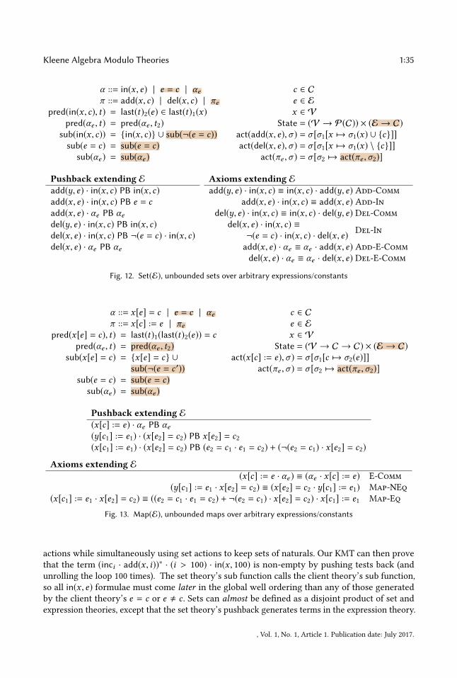
Kleene Algebra Modulo Theories 1:35
α ::= in(x , e) | e = c | αeπ ::= add(x , c) | del(x , c) | πe
pred(in(x , c), t) = last(t)2(e) ∈ last(t)1(x)pred(αe , t) = pred(αe , t2)
sub(in(x , c)) = {in(x , c)} ∪ sub(¬(e = c))sub(e = c) = sub(e = c)
sub(αe ) = sub(αe )
c ∈ Ce ∈ Ex ∈ V
State = (V → P(C)) × (E → C)act(add(x , e),σ ) = σ [σ1[x 7→ σ1(x) ∪ {c}]]act(del(x , e),σ ) = σ [σ1[x 7→ σ1(x) \ {c}]]
act(πe ,σ ) = σ [σ2 7→ act(πe ,σ2)]
Pushback extending Eadd(y, e) · in(x , c) PB in(x , c)add(x , e) · in(x , c) PB e = cadd(x , e) · αe PB αedel(y, e) · in(x , c) PB in(x , c)del(x , e) · in(x , c) PB ¬(e = c) · in(x , c)del(x , e) · αe PB αe
Axioms extending Eadd(y, e) · in(x , c) ≡ in(x , c) · add(y, e) Add-Comm
add(x , e) · in(x , c) ≡ add(x , e) Add-Indel(y, e) · in(x , c) ≡ in(x , c) · del(y, e) Del-Comm
del(x , e) · in(x , c) ≡¬(e = c) · in(x , c) · del(x , e) Del-In
add(x , e) · αe ≡ αe · add(x , e) Add-E-Commdel(x , e) · αe ≡ αe · del(x , e) Del-E-Comm
Fig. 12. Set(E), unbounded sets over arbitrary expressions/constants
α ::= x[e] = c | e = c | αeπ ::= x[c] := e | πe
pred(x[e] = c), t) = last(t)1(last(t)2(e)) = cpred(αe , t) = pred(αe , t2)
sub(x[e] = c) = {x[e] = c} ∪sub(¬(e = c ′))
sub(e = c) = sub(e = c)sub(αe ) = sub(αe )
c ∈ Ce ∈ Ex ∈ V
State = (V → C → C) × (E → C)act(x[c] := e),σ ) = σ [σ1[c 7→ σ2(e)]]
act(πe ,σ ) = σ [σ2 7→ act(πe ,σ2)]
Pushback extending E(x[c] := e) · αe PB αe(y[c1] := e1) · (x[e2] = c2) PB x[e2] = c2(x[c1] := e1) · (x[e2] = c2) PB (e2 = c1 · e1 = c2) + (¬(e2 = c1) · x[e2] = c2)
Axioms extending E(x[c] := e · αe ) ≡ (αe · x[c] := e) E-Comm
(y[c1] := e1 · x[e2] = c2) ≡ (x[e2] = c2 · y[c1] := e1) Map-NEq(x[c1] := e1 · x[e2] = c2) ≡ ((e2 = c1 · e1 = c2) + ¬(e2 = c1) · x[e2] = c2) · x[c1] := e1 Map-Eq
Fig. 13. Map(E), unbounded maps over arbitrary expressions/constants
actions while simultaneously using set actions to keep sets of naturals. Our KMT can then provethat the term (inci · add(x , i))∗ · (i > 100) · in(x , 100) is non-empty by pushing tests back (andunrolling the loop 100 times). The set theory’s sub function calls the client theory’s sub function,so all in(x , e) formulae must come later in the global well ordering than any of those generatedby the client theory’s e = c or e , c . Sets can almost be de�ned as a disjoint product of set andexpression theories, except that the set theory’s pushback generates terms in the expression theory.
, Vol. 1, No. 1, Article 1. Publication date: July 2017.

1:36 Ryan Becke�, Eric Campbell, and Michael Greenberg
α ::= ©a | a S b | aπ ::= πT
sub(©a) = {©a} ∪ sub(a)sub(a S b) = {a S b} ∪ sub(a) ∪ sub(b)act(π ,σ ) = act(π ,σ )
a = ¬ © ¬aa B b = a S b +�astart = ¬ © 1♦a = 1 S a
�a = ¬♦¬aPushback extending T
π · ©a PB a
π · a PB•T a′ · π π · b PB•T b ′ · ππ · (a S b) PB b ′ + a′ · (a S b)
State = StateTpred(©a, 〈σ , l〉)) = falsepred(©a, t 〈σ , l〉)) = pred(a, t)pred(a S b, 〈σ , l〉) = pred(b, 〈σ , l〉)pred(a S b, t 〈σ , l〉) = pred(b, t 〈σ , l〉) ∨
(pred(a, t 〈σ , l〉) ∧ pred(a S b, t))Axioms extending T
inherited from T©(a · b) ≡ ©a · ©b LTL-Last-Dist-Seq©(a + b) ≡ ©a +©b LTL-Last-Dist-Plus
1 ≡ 1 LTL-WLast-Onea S b ≡ b + a · ©(a S b) LTL-Since-Unroll
¬(a S b) ≡ (¬b) B (¬a · ¬b) LTL-Not-Sincea ≤ a · b → a ≤ �b LTL-Induction
�a ≤ ♦(start · a) LTL-Finite
Fig. 14. LTLf (T ), linear temporal logic on finite traces over an arbitrary theory
4.5 Unbounded mapsMaps aren’t much di�erent from sets; rather than having simple membership tests, we insteadcheck to see whether a given key maps to a given constant (Figure 13). Our writes use constant keysand expression values, while our reads use variable keys but constant values. We could have �ippedthis arrangement—writing to expression keys and reading from constant ones—but we cannot allowboth reads and writes to expression keys. Doing so would allow us to compare variables, putting usin the realm of context-free languages and foreclosing on the possibility of a complete theory. Wecould add other operations (at the cost of even more equational rules/pushback entries), like theability to remove keys from maps or to test whether a key is in the map or not. Just as for Set(E),we must put all x[e] = c and x[e] , c formulae later in the global well ordering than any of thosegenerated by the client theory’s e = c or e , c .
4.6 LTLfThe most interesting higher-order theory we present is that for past-time linear temporal logic on�nite traces, LTLf (Figure 14). Our theory of LTLf is itself parameterized on a theory T , whichintroduces its own predicates and actions—any T predicate can appear inside of LTLf ’s predicates.
LTLf only needs two predicates: ©a, pronounced “last a”, means a held in the prior state; anda S b, pronounced “a since b”, means b held at some point in the past, and a has held since then.There is a slight subtlety around the beginning of time: we say that ©a is false at the beginning(what can be true in a state that never happened?), and a S b degenerates to b at the beginning oftime. The last and since predicates together are enough to encode the rest of LTLf ; encodings aregiven below the syntax.
The pred de�nitions mostly defer to the client theory’s de�nition of pred (which may recursivelyreference the LTLf pred function), unrolling S as it goes (LTL-Since-Unroll). The pushbackoperation uses inference rules: to push back S, we unroll a S b into a · ©(a S b) + b; pushing lastthrough an action is easy, but pushing back a or b recursively uses the PB• judgment. Adding theserules leaves our judgments monotonic, and if π · a PB• x , then x =
∑aiπ (Lemma 3.34).
, Vol. 1, No. 1, Article 1. Publication date: July 2017.

Kleene Algebra Modulo Theories 1:37
α ::= f = vπ ::= f ← v
sub(α) = {α }pred(f = v, t) = last(t). f = vPushbackf ← v · f = v PB 1f ← v · f = v ′ PB 0 when v , v ′f ′← v · f = v PB f = v
F = packet �eldsV = packet �eld values
State = F→ Vact(f ← v,σ ) = σ [f 7→ v]
Axiomsf ← v · f ′ = v ′ ≡ f ′ = v ′ · f ← v PA-Mod-Comm
f ← v · f = v ≡ f ← v PA-Mod-Filterf = v · f = v ′ ≡ 0, if v , v ′ PA-Contra∑
v f = v ≡ 1 PA-Match-All
Fig. 15. Tracing NetKAT a/k/a NetKAT without dup
The equivalences given are borrowed from Temporal NetKAT [8] and the deductive completenessresult is borrowed from Campbell’s undergraduate thesis, which proves deductive completenessfor an axiomatic framing and then relates those axioms to our equations [10].
4.7 Tracing NetKATNetKAT de�nes a KMT over packets, which we model as functions from packet �elds to values (Fig-ure 15). NetKAT could, in principle, be implemented as a particular instance of BitVec (Section 4.1),but we present it in full in order to simplify Temporal NetKAT (Section 4.8).
Our trace-based strategy for the semantics means we have a slightly di�erent model fromconventional NetKAT [1]. NetKAT, like KAT+B! [29], normally merges adjacent writes. If the policyanalysis demands reasoning about the history of packets traversing the network—reasoning, forexample, about which routes packets actually take—the programmer must insert dup commands torecord relevant moments in time. Typically, dups are automatically inserted at the topology level, i.e.,before a packet enters a switch, we record its state by running dup. From our perspective, NetKATvery nearly has a tracing semantics, but the traces are selective. If we put an implicit dup beforeevery �eld update, NetKAT has our tracing semantics. The upshot is that our “tracing NetKAT” hasa slightly di�erent equational theory from conventional NetKAT, rejecting the following NetKATlaws as unsound for trace semantics:
f = v · f ← v ≡ f = v PA-Filter-Modf ← v · f ← v ′ ≡ f ← v ′ PA-Mod-Mod
f ← v · f ′← v ′ ≡ f ′← v ′ · f ← v PA-Mod-Mod-Comm
In principle, one can abstract our semantics’ traces to �nd the more restricted NetKAT traces, butwe can’t o�er any formal support in our framework for abstracted reasoning. Just as for BitVec, Itis possible that ideas from Kozen and Mamouras could apply here [33]; see Section 7.
4.8 Temporal NetKATWe can derive Temporal NetKAT as LTLf (NetKAT), i.e., LTLf instantiated over tracing NetKAT;the combination yields precisely the system described in the Temporal NetKAT paper [8]. Since ourLTLf theory can now rely on Campbell’s proof of deductive completeness for LTLf [10], we canautomatically derive a stronger completeness result for Temporal NetKAT, which was completeonly for “network-wide” policies, i.e., those with start at the front.
, Vol. 1, No. 1, Article 1. Publication date: July 2017.

1:38 Ryan Becke�, Eric Campbell, and Michael Greenberg
α ::= x < nπ ::= x := min+(®x)
pred(x < n, t) = last(t)(x) < nsub(x < n) = {xi < m | m ≤ n,xi ∈ V}
act(x := min+(®x),σ ) = σ [x 7→ 1 +min(σ (®x))]
n ∈ N ∪ {∞}x ∈ V
State = V → N
Pushback axioms are identical to pushbackx := min+(®x) · (x < ∞) PB Σi (xi < ∞)x := min+(®x) · (x < n) PB Σi (xi < n − 1)
Fig. 16. SP, shortest paths in a graph
α ::= C0 < n | C1 | failR1,R2 R = Routersπ ::= updateC L = R × R Links
pred(C1, t) = last(t)1(C)1 n ∈ Npred(C0 < n, t) = last(t)1(C)0 < n x ∈ Rpred(failR1,R2 , t) = last(t)2(R1,R2) State = R→ N × {true, false}
sub(failR1,R2 ) = {failR1,R2 } × L→ {true, false}sub(C1) = {A1,B1, failA,C , failB,C }
sub(C0 < n) = {A0 < n − 1,B0 < n − 1,A1,B1, failA,C , failB,C }
act(updateC),σ ) = σ
C 7→(1 + σ (B)0, true) path(B)(1 + σ (A)0, true) else if path(A)(σ (C)0,σ (C)1) otherwise
where path(X ) = σ (X )1 ∧ σ ((X ,C))1
Pushback axioms are identical to pushback(π · failR1,R2 ) PB failR1,R2(updateC · D1) PB D1(updateC ·C1) PB ¬failA,C · A1 + failB,C · B1(updateC · D0 < n) PB (D < n)(updateC ·C0 < n) PB ¬failA,C · (¬B1 + failB,C ) · A1 · (A0 < n − 1) +
¬failB,C · B1 · (B0 < n − 1)
Fig. 17. BGP, protocol theory for router C from the network in Figure 2
4.9 Distributed routing protocolsThe theory for naturals with the min+ operator used for shortest path routing is shown in Figure 16.The theory is similar to the IncNat theory but for some minor di�erences. First, the domain is nowover N ∪ {∞}. Second, there is a new axiom and pushback relation relating min+ to a test of theform x < n. Third, the subterms function is now de�ned in terms of all other variables, which arein�nite in principle but �nite in any given term (e.g., the number of routers in a given network).
The theory for the BGP protocol instance with local router policy described in Figure 2 is nowshown in Figure 17. For brevity, we only show the theory for router C in the network. The statehas two parts: the �rst part maps each router to a pair of a natural number describing the pathlength to the destination for that router, and a boolean describing whether or not the router has aroute to the destination; the second part maps links to a boolean representing whether the link is
, Vol. 1, No. 1, Article 1. Publication date: July 2017.

Kleene Algebra Modulo Theories 1:39
up or not. We require new axioms corresponding to each of the pushback operations shown. Theaction updateC commutes with unrelated tests, and otherwise behaves as described in Section 2.
5 AUTOMATAWhile the deductive completeness proof from Section 3 gave a way to determine equivalence ofKAT terms through a normalization rewriting, using such rewriting-based proofs as the basis of adecision procedure would be impractical. But just as pushback gave us a novel completeness proof,it can also help us develop an automata-theoretic account of equivalence.
Our automata theory is heavily based on previous work on Antimirov partial derivatives [4] andNetKAT’s compiler [50]. We must diverge from prior work, though, to account for client theorypredicates that depend on more than the last state of the trace. Our solution is adapted from thecompilation strategy from Temporal NetKAT [8]: to construct an automaton for a term in a KMT,we build two separate automata—one for the policy fragment of the term and one for each predicatethat occurs therein—and combine the two in a specialized intersection operation.
5.1 KMT automata, formally and by exampleA KMT automaton is a 5-tuple (S, s0, ϵ,δ ,δ0), where: the set of automata states S identi�es non-initial states (unrelated to State); the initial state s0 is distinguished from those in S ; the acceptancefunction ϵ : S → P(State) is a function identifying which theory states (in State) are acceptedin each automaton state s ∈ S ; the transition function δ : S → State → P(S × Log) identi�essuccessor states given an automaton and a single KMT state; and the initial transition functionδ0 : Trace→ P(S × State) looks at a trace and identi�es a set of successor states. Intuitively, theautomata match traces, which are sequences of log entries: 〈σ0,π1〉 . . . 〈σn ,πn〉.
Consider the KMT automaton shown in Figure 18 (right) for the term incx ∗ · ♦x > 2 taken fromthe LTLf (IncNat) theory. The automaton would accept a trace of the form: 〈[x 7→ 1,⊥]〉〈[x 7→2, incx ]〉〈[x 7→ 3], incx 〉. Informally, the automaton starts in the initial state s0, which is (0,0) (theparticular value used to represent the state, tuples in this case, is unimportant), and moves to state(1,1) for the transition labeled with x > 0. This predicate describes a set of theory states includingthe one where x is 1. The automaton then moves to state (3,1) and then (4,1) unconditionally for theincx action, which corresponds to actions in the log entries of the trace. The acceptance functionassigns state (4,1) the condition 1, meaning that all theory states are accepted; no other states areaccepting, i.e., the acceptance function assigns them the condition 0.
The transition function δ takes an automaton state S and a KMT state and maps them to a setof new pairs of automaton state and and KMT log items (a KMT state/action pair). In the �gure,we transitions as arcs between states with a pair of a KMT test and a primitive KMT action. Forexample, the transition from state (1,1) to (2,1) is captured by the term 1 · incx , which captures thee�ect of updating the theory domain state in the log by incrementing the value of x . Finally, theinitial transition function δ0 is similar to δ , but accounts for the fact that there may be an initialtrace of log items in the initial state (as in LTLf ). For example, the transition from (0,0) to (4,1) istaken if either the initial trace has x > 2 in the current state or at some point in the past (representedwith multiple transitions). Representing initial transitions separately allows us to compose KMTautomata, overcoming the limited “network-wide” completeness in Temporal NetKAT [8].
Taken all together, our KMT automaton captures the fact that there are 4 interesting cases forthe term incx ∗ · ♦x > 2. If the program trace already had x > 2 at some point in the past or hasx > 2 in the current state, then we move to state (4,1) and will accept the trace regardless of howmany increment commands are executed in the future. If the initial trace has x > 1, then we moveto state (3,1). If we see at least one more increment command, then we move to state (4,1) where the
, Vol. 1, No. 1, Article 1. Publication date: July 2017.
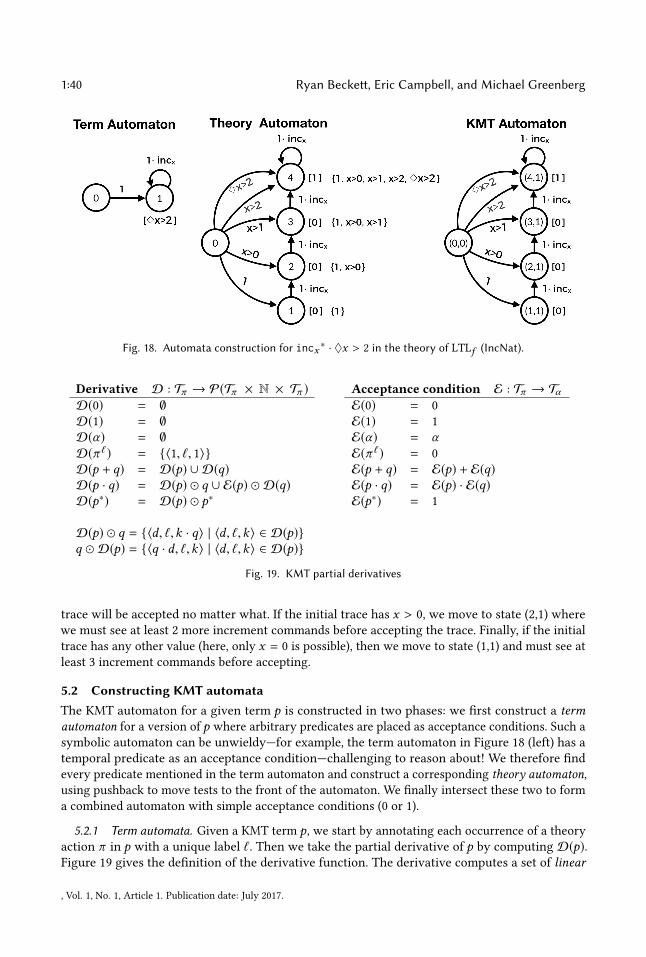
1:40 Ryan Becke�, Eric Campbell, and Michael Greenberg
Fig. 18. Automata construction for incx ∗ · ♦x > 2 in the theory of LTLf (IncNat).
Derivative D : Tπ → P(Tπ × N × Tπ )D(0) = ∅D(1) = ∅D(α) = ∅D(π `) = {〈1, `, 1〉}D(p + q) = D(p) ∪ D(q)D(p · q) = D(p) � q ∪ E(p) � D(q)D(p∗) = D(p) � p∗
D(p) � q = {〈d, `,k · q〉 | 〈d, `,k〉 ∈ D(p)}q � D(p) = {〈q · d, `,k〉 | 〈d, `,k〉 ∈ D(p)}
Acceptance condition E : Tπ → TαE(0) = 0E(1) = 1E(α) = αE(π `) = 0E(p + q) = E(p) + E(q)E(p · q) = E(p) · E(q)E(p∗) = 1
Fig. 19. KMT partial derivatives
trace will be accepted no matter what. If the initial trace has x > 0, we move to state (2,1) wherewe must see at least 2 more increment commands before accepting the trace. Finally, if the initialtrace has any other value (here, only x = 0 is possible), then we move to state (1,1) and must see atleast 3 increment commands before accepting.
5.2 Constructing KMT automataThe KMT automaton for a given term p is constructed in two phases: we �rst construct a termautomaton for a version of p where arbitrary predicates are placed as acceptance conditions. Such asymbolic automaton can be unwieldy—for example, the term automaton in Figure 18 (left) has atemporal predicate as an acceptance condition—challenging to reason about! We therefore �ndevery predicate mentioned in the term automaton and construct a corresponding theory automaton,using pushback to move tests to the front of the automaton. We �nally intersect these two to forma combined automaton with simple acceptance conditions (0 or 1).
5.2.1 Term automata. Given a KMT term p, we start by annotating each occurrence of a theoryaction π in p with a unique label `. Then we take the partial derivative of p by computing D(p).Figure 19 gives the de�nition of the derivative function. The derivative computes a set of linear
, Vol. 1, No. 1, Article 1. Publication date: July 2017.

Kleene Algebra Modulo Theories 1:41
forms—tuples of the form 〈d, `,k〉. There will be exactly one such tuple for each unique label `, andeach label will represent a single state in the automaton. The acceptance function for state ` isgiven by E(k). To compute the transition function, for each such tuple, we then compute D(k),which will return another set of tuples. For each such tuple: 〈d ′, `′,k ′〉 ∈ D(k), we add a transitionfrom state ` to state `′ labeled with the term d ′ · π `′ . The d part is a predicate identifying when thetransition activates, while the k part is the “continuation”, i.e., what else in the term can be run.
For example, the term incx ∗ · ♦x > 2, is �rst labeled as (incx 1)∗ · ♦x > 2. We then computeD((incx 1)∗ · ♦x > 2) = {〈1, inc1, (inc1x )∗ · ♦x > 2〉}. Taking the derivative of the resulting value,(inc1x )∗ · ♦x > 2, results in the same tuple, so there is a single transition from state 1 to itself,which has its transition labeled with 1 · inc1x . The acceptance function for this state is given byE((inc1x )∗ · ♦x > 2) = ♦x > 2. The resulting automaton is shown in Figure 18 (left). We add atransition from the initial state 0 to state 1 to represent the initial transition function.
5.2.2 Theory automata. Once we’ve constructed the term automaton, we construct theoryautomata for each predicate that appears in an acceptance or transition condition of the termautomaton. The theory automaton for a predicate a tracks whether a holds so far in a trace, givensome initial trace and a sequence of primitive actions. We use pushback (Section 3.3.2) to generatethe transition relation of the theory automaton, since the pushback exactly characterizes the e�ectof a primitive action π on predicates a: to determine if a predicate α is true after some action a, wecan instead check if b is true in the previous state when we know that π · a PB• b · π .
While a KMT may include an in�nite number of primitive actions (e.g., x := n for n ∈ N inIncNat), any given term only has �nitely many. For incx ∗ · ♦x > 2, there is only a single primitiveaction: incx . For each such action π that appears in the term and each subterm s of the test ♦x > 2,we compute the pushback of π and s .
For non-initial states, we maintain a labeling function L, which identi�es the set subterms ofthe top-level predicate a that hold in that state. For each subterm s , we add a transition 1 · π fromstates x to y if s ∈ L(y) and π · s PB• b · π , and b is true given the labeling L(x). For example,in the theory automaton show in Figure 18 (middle), there is a transition from state 3 to state 4for action incx . State 4 is labeled with {1,x > 0,x > 1,x > 2,♦x > 2} and state 3 is labeled with{1,x > 0,x > 1}. We compute incx · ♦x > 2 PB (♦x > 2 + x > 1). Therefore, ♦x > 2 should belabeled in state 4 if and only if either ♦x > 2 is labeled in state 3 or x > 1 is labeled in state 3. Sincestate 3 is labeled with x > 1, it follows that state 4 must be labeled with ♦x > 2.
We must again treat the initial state specially: there is a transition for each satis�able combinationof subterms of the top-level predicate a; the transition leads to a state labeled with all the othersubterms implied by this subterm. For example, if a = ♦x > 2 and we are considering the subtermx > 2, then we know that if x > 2, then x > 1 and ♦x > 2 as well, so we construct an edge toa node with all three in its label. We can discover these implications by calling out to the clienttheory to check validity of the implication.
Finally, a state is accepting in the theory automaton if it is labeled with the top-level predicatefor which the automaton was built. For example, state 4 is accepting (with acceptance function [1]),since it is labeled with ♦x > 2.
5.3 KMT automataWe can combine the term and theory automata to create a KMT automaton. The idea is to intersectthe two automata together, and replace instances of theory tests in the acceptance and transitionfunctions of the term automaton with the acceptance condition for the given state in the theoryautomata. For example, in Figure 18, the combined automata (right) replaces instances of the ♦x > 2condition in state 1 of the term automaton, with the acceptance condition from the corresponding
, Vol. 1, No. 1, Article 1. Publication date: July 2017.

1:42 Ryan Becke�, Eric Campbell, and Michael Greenberg
module rec IncNat : THEORY = struct
module K = KAT(IncNat) (* recursive self reference to generated KMT *)
type a = Gt of string ∗ int (* alpha ::= x > n *)
type p = string (* pi ::= inc x *)
let parse name es = (* extensible parser *)
match name, es with| "inc", [EId s1]→ Action s1
| ">", [EId s1; EId s2]→ Test (Gt(s1, int_of_string s2))| _, _→ failwith "Cannot create theory object"
let rec subterms (a : K.a) = (* for maximal term ordering/pushback *)
match a with
| Gt(_,0)→ PSet.empty| Gt(v,i)→ PSet.add a (subterms (Gt(v,i−1)))let push_back (x : K.p) (a : K.a) = (* pushback on theory terms *)
match a with
| Gt(_,0)→ PSet.singleton a
| Gt (y,v) when x = y→ PSet.add (K.theory a) (subterms (Gt(y,i−1)))| _→ PSet.singleton (K.theory a)let satisfiable (t : K.test) = ... (* decision procedure *)
end
module K = KAT(LTLF(IncNat)) (* build KAT from LTLF on incrementing naturals *)
module A = Automata(K) (* construct automata for our KAT *)
let main () =let a = K.parse "inc(x)*; since(true, x>2)" in
let b = K.parse "since(true, x>2); inc(x)* + inc(x)*; x > 2; inc(x)*" in
assert (A.equivalent (A.of_term a) (A.of_term b))
Fig. 20. Simplified example and use of an implementation of IncNat in OCaml.
state in the theory automaton. In state (3,1) this is true, while in states (2,1) and (1,1) this is false.For transitions with the same action π , the intersection takes the conjunction of each edge’s tests.
5.4 Equivalence checkingDue to space constraints, we only brie�y summarize the ideas behind equivalence checking. Tocheck the equivalence of two KMT terms p and q, we �rst convert both p and q to their respective(symbolic) automata. We then determinize the automata, using an algorithm based on minterms [14],to ensure that all transition predicates are disjoint, and the typical automata powerset construction.We then check for a bisimulation between the two automata [9, 21, 42] by checking if, given anytwo bisimilar states, all transitions from the states lead to bisimilar states.
6 IMPLEMENTATIONWe have implemented our ideas in OCaml. Users of the library write theory implementations byde�ning new OCaml modules that de�ne the types of actions and tests, and functions for parsing,
, Vol. 1, No. 1, Article 1. Publication date: July 2017.
Kleene Algebra Modulo Theories 1:43
computing subterms, calculating pushback for primitive actions and predicates, and deciding theorysatis�ability functions.
Figure 20 shows an example library implementation of the theory of naturals. The implementationstarts by de�ning a new, recursive module called IncNat. Recursive modules are useful, becauseit allows the author of the module to access the �nal KAT functions and types derived afterinstantiating KA with their theory while still implementing the theory itself. For example, themodule K on the second line gives us a recursive reference to the resulting KAT instantiated with theIncNat theory; such self-reference is key for theories like LTLf , which must embed KAT predicatesinside of temporal operators and call the KAT pushback while performing its own (Section 4.6). Inthe example, the user then de�nes two types: the type a for tests, and the type p for actions. Testsare of the form x > n where variable names are represented with strings, and values with OCamlints. The only action is to increment the variable, so we simply need to know the variable name.
The �rst function, parse, allows the library author to extend the KAT parser (if desired) toinclude new kinds of tests and actions in terms of in�x and named operators. In this example, theparser is extended to read actions of the form inc(x) and tests of the form x > c . The other functions:subterms and push_back follow from the KMT theory directly. Finally, the user must implement afunction that checks satis�ability of a theory test. To use a theory, one need only instantiate theappropriate modules: The module K instantiates LTLF over our theory of incrementing naturals;the module A gives us an automata theory for K. Checking language equivalence is then simply amatter of reading in a term, constructing an automata and checking equivalence. In practice, ourimplementation uses several optimizations, with the two most prominent being (1) hash-consing allKAT terms to ensure fast set operations, and (2) lazy construction and exploration of automata forequivalence checking. Our satis�ability procedure for IncNat makes a heuristic decision betweenusing our incomplete custom solver or Z3 [17]—our solver is much faster on its restricted domain.
7 RELATEDWORKKozen and Mamouras’s Kleene algebra with equations [33] is perhaps the most closely related work:they also devise a framework for proving extensions of KAT sound and complete. Both their workand ours use rewriting to �nd normal forms and prove deductive completeness. Their rewritingsystems work on mixed sequences of actions and predicates, but they they can only delete thesesequences wholesale or replace them with a single primitive action or predicate; our rewritingsystem (pushback) only works on predicates due to the trace semantics that preserves the orderof actions, but pushing a test back can yield something larger than a single primitive predicate.In the big picture, Kozen and Mamouras can accommodate equations that combine actions, likethose that eliminate redundant writes in KAT+B! and NetKAT [1, 29], while we can accommodatecomplex predicates and their interaction with actions, like those found in Temporal NetKAT [8] orthose produced by the theory combinators in Section 4. A trace semantics like the one described inthis paper is used in previous work on KAT as well [25, 32].
Coalgebra provides a general framework for reasoning about state-based systems [44, 49], whichhas proven useful in the development of automata theory for KAT extensions. Although we do notexplicitly develop the connection in this paper, Kleene algebra modulo theories uses tools similarto those used in coalgebraic approaches, and one could perhaps adapt our scheme to that setting.
Propositional dynamic logic (PDL) [20] gives an alternative approach to reasoning about regularlystructured programs. It is a decidable logic with a complete axiomatization [41] that can embedKleene algebra. However, like KAT, PDL is purely propositional and does not address the problemof reasoning within a particular domain of interest. Further PDL comes with a di�erent set oftradeo�s: while KAT is PSPACE complete, PDL is known to be EXPTIME-complete. von Karger
, Vol. 1, No. 1, Article 1. Publication date: July 2017.

1:44 Ryan Becke�, Eric Campbell, and Michael Greenberg
[53] shows how Kleene algebra can be extended with domain and codomain operators to give analgebraic approach to PDL, however he does not prove that the extension is complete, and stillcannot reason about particular theories.
Our work is loosely related to Satis�ability Modulo Theories (SMT) [18]. The high-level motiva-tion is the same—to create an extensible framework where custom theories can be combined [38]and used to increase the expressiveness and power [51] of the underlying technique (SAT vs. KA).However, the speci�cs vary greatly—while SMT is used to reason about the satis�ability of aformula, KMT is used to reason about the structure of the program and its interaction with tests.
The pushback requirement detailed in this paper is strongly related to the classical notion ofweakest precondition [6, 19, 45]. However, automatic weakest precondition generation is generallylimited in the presence of loops in while-programs. While there has been much work on loopinvariant inference [23, 24, 26, 31, 40, 47], the problems remains undecidable in most cases. However,the pushback restrictions of “growth” of terms makes it possible for us to automatically lift theweakest precondition generation to loops in KAT. In fact, this is exactly what the normalizationproof does when lifting tests out of the Kleene star operator.
The automata representation described in Section 5 is based on prior work on symbolic au-tomata [14, 42, 50]. One notable di�erence with previous work is that the construction of automatain our setting is complicated by the fact that theories can introduce predicates that take into accountthe entire view of the previous trace. The separate account of theory and term automata we presenttakes this into account is based on ideas in Temporal NetKAT [8].
8 CONCLUSIONKleene algebra modulo theories (KMT) is a new framework for extending Kleene algebra withtests with the addition of actions and predicates in a custom domain. KMT uses an operation thatpushes tests back through actions to go from a decidable client theory to a domain-speci�c KMT.Derived KMTs are sound and complete equational theory sound with respect to a trace semantics,and automatically construct automata-theoretic decision procedures for the KMT. Our theoreticalframework captures common use cases in the form of theories for bitvectors, natural numbers,unbounded sets and maps, networks, and temporal logic.
ACKNOWLEDGMENTSDave Walker and Aarti Gupta provided valuable advice. Ryan Beckett was supported by NSF CNSaward 1703493.
REFERENCES[1] Carolyn Jane Anderson, Nate Foster, Arjun Guha, Jean-Baptiste Jeannin, Dexter Kozen, Cole Schlesinger, and David
Walker. Netkat: Semantic foundations for networks. In Proceedings of the 41st ACM SIGPLAN-SIGACT Symposium onPrinciples of Programming Languages, POPL ’14, pages 113–126, New York, NY, USA, 2014. ACM.
[2] M Anderson. Time warner cable says outages largely resolved. http://www.seattletimes.com/business/time-warner-cable-says-outages-largely-resolved, 2014.
[3] Allegra Angus and Dexter Kozen. Kleene algebra with tests and program schematology. Technical report, CornellUniversity, Ithaca, NY, USA, 2001.
[4] Valentin Antimirov. Partial derivatives of regular expressions and �nite automata constructions. Theoretical ComputerScience, 155:291–319, 1995.
[5] Mina Tahmasbi Arashloo, Yaron Koral, Michael Greenberg, Jennifer Rexford, and David Walker. Snap: Statefulnetwork-wide abstractions for packet processing. In Proceedings of the 2016 ACM SIGCOMM Conference, SIGCOMM’16, pages 29–43, New York, NY, USA, 2016. ACM.
[6] Mike Barnett and K. Rustan M. Leino. Weakest-precondition of unstructured programs. In Proceedings of the 6th ACMSIGPLAN-SIGSOFT Workshop on Program Analysis for Software Tools and Engineering, PASTE ’05, pages 82–87, NewYork, NY, USA, 2005. ACM.
, Vol. 1, No. 1, Article 1. Publication date: July 2017.

Kleene Algebra Modulo Theories 1:45
[7] Adam Barth and Dexter Kozen. Equational veri�cation of cache blocking in lu decomposition using kleene algebrawith tests. Technical report, Cornell University, 2002.
[8] Ryan Beckett, Michael Greenberg, and David Walker. Temporal netkat. In Proceedings of the 37th ACM SIGPLANConference on Programming Language Design and Implementation, PLDI ’16, pages 386–401, New York, NY, USA, 2016.ACM.
[9] Filippo Bonchi and Damien Pous. Checking nfa equivalence with bisimulations up to congruence. SIGPLAN Not., 48(1):457–468, January 2013.
[10] Eric Hayden Campbell. In�niteness and linear temporal logic: Soundness, completeness, and decidability. Undergrad-uate thesis, Pomona College, 2017.
[11] Ernie Cohen. Using kleene algebra to reason about concurrency control. Technical report, Telcordia, 1994.[12] Ernie Cohen. Hypotheses in kleene algebra, 1994. URL http://citeseerx.ist.psu.edu/viewdoc/summary?doi=10.1.1.56.
6067.[13] Ernie Cohen. Lazy caching in kleene algebra, 1994. URL http://citeseerx.ist.psu.edu/viewdoc/summary?doi=10.1.1.57.
5074.[14] Loris D’Antoni and Margus Veanes. Minimization of symbolic automata. SIGPLAN Not., 49(1):541–553, January 2014.
ISSN 0362-1340.[15] Giuseppe De Giacomo and Moshe Y Vardi. Linear temporal logic and linear dynamic logic on �nite traces. In IJCAI’13
Proceedings of the Twenty-Third international joint conference on Arti�cial Intelligence, pages 854–860. Association forComputing Machinery, 2013.
[16] Giuseppe De Giacomo, Riccardo De Masellis, and Marco Montali. Reasoning on ltl on �nite traces: Insensitivity toin�niteness. In AAAI, pages 1027–1033. Citeseer, 2014.
[17] Leonardo De Moura and Nikolaj Bjørner. Z3: An e�cient smt solver. In Proceedings of the Theory and Practice of Software,14th International Conference on Tools and Algorithms for the Construction and Analysis of Systems, TACAS’08/ETAPS’08,pages 337–340, Berlin, Heidelberg, 2008. Springer-Verlag.
[18] Leonardo De Moura and Nikolaj Bjørner. Satis�ability modulo theories: Introduction and applications. Commun.ACM, 54(9):69–77, September 2011.
[19] Edsger W. Dijkstra. Guarded commands, nondeterminacy and formal derivation of programs. Commun. ACM, 18(8):453–457, August 1975.
[20] Michael J. Fischer and Richard E. Ladner. Propositional dynamic logic of regular programs. Journal of Computer andSystem Sciences, 18(2):194 – 211, 1979.
[21] Nate Foster, Dexter Kozen, Matthew Milano, Alexandra Silva, and Laure Thompson. A coalgebraic decision procedurefor netkat. In Proceedings of the 42Nd Annual ACM SIGPLAN-SIGACT Symposium on Principles of ProgrammingLanguages, POPL ’15, pages 343–355, New York, NY, USA, 2015. ACM.
[22] Nate Foster, Dexter Kozen, Konstantinos Mamouras, Mark Reitblatt, and Alexandra Silva. Probabilistic netkat. In PeterThiemann, editor, Programming Languages and Systems: 25th European Symposium on Programming, ESOP 2016, Heldas Part of the European Joint Conferences on Theory and Practice of Software, ETAPS 2016, Eindhoven, The Netherlands,April 2–8, 2016, Proceedings, pages 282–309, Berlin, Heidelberg, 2016. Springer Berlin Heidelberg.
[23] Carlo A. Furia and Bertrand Meyer. Inferring loop invariants using postconditions. CoRR, abs/0909.0884, 2009.[24] Carlo Alberto Furia and Bertrand Meyer. Inferring Loop Invariants Using Postconditions, pages 277–300. Springer Berlin
Heidelberg, Berlin, Heidelberg, 2010.[25] Murdoch J. Gabbay and Vincenzo Ciancia. Freshness and name-restriction in sets of traces with names. In Proceedings
of the 14th International Conference on Foundations of Software Science and Computational Structures: Part of the JointEuropean Conferences on Theory and Practice of Software, FOSSACS’11/ETAPS’11, pages 365–380, Berlin, Heidelberg,2011.
[26] Juan P. Galeotti, Carlo A. Furia, Eva May, Gordon Fraser, and Andreas Zeller. Automating full functional veri�cationof programs with loops. CoRR, abs/1407.5286, 2014. URL http://arxiv.org/abs/1407.5286.
[27] Phillipa Gill, Navendu Jain, and Nachiappan Nagappan. Understanding network failures in data centers: Measurement,analysis, and implications. In SIGCOMM, 2011.
[28] Joanne Godfrey. The summer of network miscon�gurations. https://blog.algosec.com/2016/08/business-outages-caused-miscon�gurations-headline-news-summer.html, 2016.
[29] Niels Bjørn Bugge Grathwohl, Dexter Kozen, and Konstantinos Mamouras. Kat + b! In Proceedings of the Joint Meetingof the Twenty-Third EACSL Annual Conference on Computer Science Logic (CSL) and the Twenty-Ninth Annual ACM/IEEESymposium on Logic in Computer Science (LICS), CSL-LICS ’14, pages 44:1–44:10, New York, NY, USA, 2014. ACM.
[30] Zeus Kerravala. What is behind network downtime? proactive steps to reduce human error and improve availabilityof networks. https://www.cs.princeton.edu/courses/archive/fall10/cos561/papers/Yankee04.pdf, 2004.
, Vol. 1, No. 1, Article 1. Publication date: July 2017.

1:46 Ryan Becke�, Eric Campbell, and Michael Greenberg
[31] Soonho Kong, Yungbum Jung, Cristina David, Bow-Yaw Wang, and Kwangkeun Yi. Automatically inferring quan-ti�ed loop invariants by algorithmic learning from simple templates. In Proceedings of the 8th Asian Conference onProgramming Languages and Systems, APLAS’10, pages 328–343, 2010.
[32] Dexter Kozen. Kleene algebra with tests and the static analysis of programs. Technical report, Cornell University,2003.
[33] Dexter Kozen and Konstantinos Mamouras. Kleene algebra with equations. In Javier Esparza, Pierre Fraigniaud, ThoreHusfeldt, and Elias Koutsoupias, editors, Automata, Languages, and Programming: 41st International Colloquium, ICALP2014, Copenhagen, Denmark, July 8-11, 2014, Proceedings, Part II, pages 280–292, Berlin, Heidelberg, 2014. SpringerBerlin Heidelberg.
[34] Dexter Kozen and Maria-Christina Patron. Certi�cation of compiler optimizations using kleene algebra with tests. InProceedings of the First International Conference on Computational Logic, CL ’00, pages 568–582, London, UK, UK, 2000.Springer-Verlag. ISBN 3-540-67797-6.
[35] Kim G Larsen, Stefan Schmid, and Bingtian Xue. Wnetkat: Programming and verifying weighted software-de�nednetworks. In OPODIS, 2016.
[36] Ratul Mahajan, David Wetherall, and Tom Anderson. Understanding BGP miscon�guration. In SIGCOMM, 2002.[37] Jedidiah McClurg, Hossein Hojjat, Nate Foster, and Pavol Černý. Event-driven network programming. In Proceedings
of the 37th ACM SIGPLAN Conference on Programming Language Design and Implementation, PLDI ’16, pages 369–385,New York, NY, USA, 2016. ACM.
[38] Greg Nelson and Derek C. Oppen. Simpli�cation by cooperating decision procedures. ACM Trans. Program. Lang.Syst., 1(2):245–257, October 1979.
[39] Juniper Networks. As the value of enterprise networks escalates, so does the need for con�guration management.https://www-935.ibm.com/services/au/gts/pdf/200249.pdf, 2008.
[40] Saswat Padhi, Rahul Sharma, and Todd Millstein. Data-driven precondition inference with learned features. InProceedings of the 37th ACM SIGPLAN Conference on Programming Language Design and Implementation, PLDI ’16,pages 42–56, New York, NY, USA, 2016.
[41] Rohit Parikh. The completeness of propositional dynamic logic. In J. Winkowski, editor, Mathematical Foundationsof Computer Science 1978: Proceedings, 7th Symposium Zakopane, Poland, September 4–8, 1978, pages 403–415, Berlin,Heidelberg, 1978.
[42] Damien Pous. Symbolic algorithms for language equivalence and kleene algebra with tests. In Proceedings of the 42NdAnnual ACM SIGPLAN-SIGACT Symposium on Principles of Programming Languages, POPL ’15, pages 357–368, NewYork, NY, USA, 2015.
[43] Yakov Rekhter and Tony Li. A Border Gateway Protocol 4 (BGP-4). RFC 1654, RFC Editor, July 1995. URL http://www.rfc-editor.org/rfc/rfc1654.txt.
[44] J. J.M.M. Rutten. Universal coalgebra: A theory of systems. Technical report, CWI (Centre for Mathematics andComputer Science), Amsterdam, The Netherlands, The Netherlands, 1996.
[45] Andrew E. Santosa. Comparing weakest precondition and weakest liberal precondition. CoRR, abs/1512.04013, 2015.[46] Cole Schlesinger, Michael Greenberg, and David Walker. Concurrent netcore: From policies to pipelines. In Proceedings
of the 19th ACM SIGPLAN International Conference on Functional Programming, ICFP ’14, pages 11–24, New York, NY,USA, 2014. ACM.
[47] Rahul Sharma and Alex Aiken. From invariant checking to invariant inference using randomized search. In Proceedingsof the 16th International Conference on Computer Aided Veri�cation - Volume 8559, pages 88–105, New York, NY, USA,2014.
[48] Simon Sharwood. Google cloud wobbles as workers patch wrong routers. http://www.theregister.co.uk/2016/03/01/google_cloud_wobbles_as_workers_patch_wrong_routers/, 2016.
[49] Alexandra Silva. Kleene coalgebra. Phd thesis, University of Minho, Braga, Portugal, 2010.[50] Ste�en Smolka, Spiridon Eliopoulos, Nate Foster, and Arjun Guha. A fast compiler for netkat. In Proceedings of the
20th ACM SIGPLAN International Conference on Functional Programming, ICFP 2015, pages 328–341, New York, NY,USA, 2015. ACM.
[51] Aaron Stump, Clark W. Barrett, David L. Dill, and Jeremy R. Levitt. A decision procedure for an extensional theory ofarrays. In LICS, 2001.
[52] Yevgenly Sverdlik. Microsoft: miscon�gured network device led to azure outage. http://www.datacenterdynamics.com/content-tracks/servers-storage/microsoft-miscon�gured-network-device-led-to-azure-outage/68312.fullarticle, 2012.
[53] Burghard von Karger. Temporal algebra. In Roland Backhouse, Roy Crole, and Jeremy Gibbons, editors, Algebraic andCoalgebraic Methods in the Mathematics of Program Construction, pages 309–385. Springer-Verlag New York, Inc., NewYork, NY, USA, 2002.
, Vol. 1, No. 1, Article 1. Publication date: July 2017.
![Encyclopaedia of Proof Systems - hansdieterhiep.nl · 15 Resolution for Modal Logic K ... Stephen Cole Kleene. ... 1952. [2]Stephen Cole Kleene. Mathematical Logic. Dover reprint](https://img.pdfslide.net/doc/110x75/5b7950d57f8b9ad77e8d4876/encyclopaedia-of-proof-systems-15-resolution-for-modal-logic-k-stephen.jpg)