S-2 -Theory of the Firm - Dartmouth Collegeecon21/x02-topic2.pdfTopic 2: Theory of the Firm Economics 21, Summer 2002 Andreas Bentz Based Primarily on Varian, Ch. 18-25 2 The Setup

DARTMOUTH COLLEGE, DEPARTMENT OF ECONOMICS ECONOMICS 21

© Andreas Bentz page 1

Dartmouth College, Department of Economics: Economics 21, SummerDartmouth College, Department of Economics: Economics 21, SummerDartmouth College, Department of Economics: Economics 21, Summer‘02‘02‘02

Topic 2: Theory of the FirmTopic 2: Theory of the Firm

Economics 21, Summer 2002Andreas Bentz

Based Primarily on Varian, Ch. 18-25

2

The SetupThe SetupA firm

produces output y, which it can sell for price p(y)» p(y) is the inverse market demand function

from quantities of inputs (factors): x1, x2, …input cost (per unit): w1, w2, …

How can this firm produce?technology

How should this firm produce?cost minimization

How much should this firm produce?profit maximization




TechnologyTechnology

Production

4

Intro: ProductionIntro: ProductionIn our problem, the firm’s production technology is given;and: the technology is independent of the market form (market structure):

in particular it has nothing to do with competition or firm behavior.



5

Production FunctionProduction FunctionA production function tells you how much output (at most) you can get from given quantities of inputs (factors).

Example (Cobb-Douglas): f(x1, x2) = x1a x2

b.

Here: x10.5 x2

0.5.

6

ShortShort--Run Production FunctionRun Production FunctionIn the short run, not all inputs can be varied: at least one input is fixed.

Suppose input 2 is fixed at x2 = x2: y = f(x1, x2)We can still vary output by varying input 1. This is the short-run production function.



7

Marginal ProductMarginal ProductSuppose input 2 is held constant: how does output change as we change input 1?

The marginal product of input 1 is the partial derivative of the production function with respect to input 1.Example: Holding x2 constant at x2 = 2, how does u change as we change x1 by a little, i.e. what is the slope of the blue line?

8

Marginal Product, cont’dMarginal Product, cont’dFormally, the marginal product of input 1 of the production function f(x1, x2) is:

That is, at which rate does output increase as this firm uses more of input 1?

1

212110x1 x

)x,x(f)x,xx(flimMP1 ∆

−∆+=

→∆1

21

x)x,x(f

∂∂

=



9

Buzz Group: Marginal ProductBuzz Group: Marginal ProductWhat is the marginal product of input 1 of the Cobb-Douglas production function

f(x1, x2) = x10.5 x2

0.5?Does the marginal product increase or decrease as the firm uses more of input 1?Answer:

MP1 = 0.5 x1-0.5 x2

0.5.This decreases as x1 increases, because its slope is negative: ∂MP1 / ∂x1 = -0.25 x1

-1.5 x20.5.

10

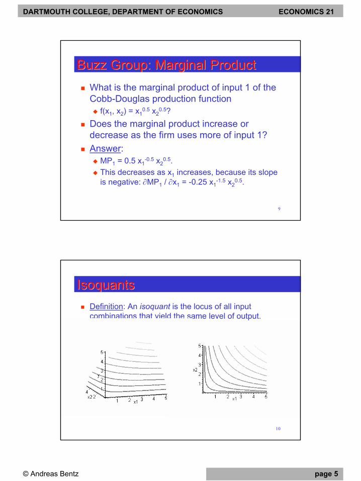
IsoquantsIsoquantsDefinition: An isoquant is the locus of all input combinations that yield the same level of output.



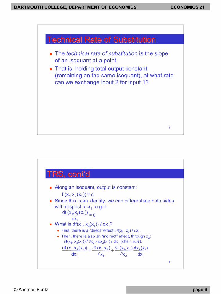
11

Technical Rate of SubstitutionTechnical Rate of SubstitutionThe technical rate of substitution is the slope of an isoquant at a point.That is, holding total output constant (remaining on the same isoquant), at what rate can we exchange input 2 for input 1?

12

TRS, cont’dTRS, cont’d

0dx

))x(x,x(df1

121 =

c))x(x,x(f 121 ≡

1

12

2

21

1

21

1

121

dx)x(dx

x)x,x(f

x)x,x(f

dx))x(x,x(df

∂∂

+∂

∂=

Along an isoquant, output is constant:

Since this is an identity, we can differentiate both sides with respect to x1 to get:

What is df(x1, x2(x1)) / dx1?First, there is a “direct” effect: ∂f(x1, x2) / ∂x1.Then, there is also an “indirect” effect, through x2: ∂f(x1, x2(x1)) / ∂x2 • dx2(x1) / dx1 (chain rule).



13

TRS, cont’dTRS, cont’dSo we know that

But we wanted to keep output constant, so

So we have:

which we can rearrange as:

2

1

MPMP−=

x)x,x(f

x)x,x(f

1

12

dx)x(dx

2

21

1

21

−=∂

∂∂

∂

1

12

2

21

1

21

1

121

dx)x(dx

x)x,x(f

x)x,x(f

dx))x(x,x(df

∂∂

+∂

∂=

0dx

))x(x,x(df1

121 =

0dx

)x(dxx

)x,x(fx

)x,x(f1

12

2

21

1

21 =∂

∂+

∂∂

14

Buzz Group: TRSBuzz Group: TRSWhat is the technical rate of substitution (slope of the isoquant) for the Cobb-Douglas production function

f(x1, x2) = x10.5 x2

0.5

… at the point x1 = x2 = 2?… at the point x1 = 4, x2 = 1 ?

(this is the same isoquant)




Firm Decisions and Firm Decisions and Market StructureMarket Structure

What to do, when.

16

Intro: Tools for Firm DecisionsIntro: Tools for Firm DecisionsHow should firms make choices (about production, input purchases, etc.)?These tools (unlike production technology) depend on market structure:

e.g. does the firm operate in a competitive market, or is it a monopolist?

For instance, we assume that the firm operates in a market, so that there are prices for inputs and output.




Firm Decisions IFirm Decisions I

Profit Maximization

18

Profit MaximizationProfit MaximizationFirms maximize profits (revenue - cost).Why?

Shareholders are interested in the value of their shares.Shares reflect the present value of the firm, that is the present discounted value of all future profits.Shareholders therefore will want management to maximize profits.(Is this really true? Can shareholders control management sufficiently? See topic 5.)



19

Short Run Profit MaximizationShort Run Profit MaximizationA (competitive) firm’s profit maximization problem is:

maxx1 p f(x1, x2) - (w1 x1 + w2 x2).The necessary (first order) condition is:

p • ∂f(x1, x2)/∂x1 - w1 = 0, or:» p • MP1 = w1

The value of the marginal product of the variable input has to be equal to that input’s price.

20

Long Run Profit MaximizationLong Run Profit MaximizationA (competitive) firm’s profit maximization problem is:

maxx1,x2 p f(x1, x2) - (w1 x1 + w2 x2).The necessary (first order) conditions are:

(i) p • ∂f(x1, x2)/∂x1 - w1 = 0, or:» p • MP1 = w1

(ii) p • ∂f(x1, x2)/∂x2 - w2 = 0, or:» p • MP2 = w2

The value of the marginal product of each input has to be equal to the input’s price.




Firm Decisions IIFirm Decisions II

Cost Minimization

22

Cost MinimizationCost MinimizationHow should a firm produce?

Given that the firm wishes to produce a certain level of output, with what combination of inputs should it produce that output?The firm should use inputs so as to minimize cost.This fits a “delegation story.”

That is, the firm solves:

y)x,x(f:.t.s

xwxwmin

21

2211x,x 21

=

+



23

Cost Min., GraphicallyCost Min., GraphicallyA firm’s cost c is:

c = w1 x1 + w2 x2» where x1, x2 are inputs at prices w1, w2

rearrange: x2 = c / w2 - (w1 / w2) x1

This is the equation for the isocost linecorresponding to cost level c.

Definition: An isocost line is the locus of input combinations that have the same cost.

24

Cost Min., Graphically, cont’dCost Min., Graphically, cont’d

Isocost lines: x2 = c / w2 - (w1 / w2) x1



25

Cost Min., Graphically, cont’dCost Min., Graphically, cont’dFirms choose to produce a given level of output (on a given isoquant) using the least cost combination of inputs (they minimize cost).

Firms choose to locate on the lowest isocost line, subject to the constraint of producing a given level of output.

Implication: TRS = - MP1 / MP2 = - w1 / w2

26

Cost Min., CalculusCost Min., CalculusWrite down the Lagrangean:

Write down the necessary (first-order) conditions:

Then solve for x1 and x2.Without a specific functional form for f(•, •) we cannot solve for x1 and x2. But the necessary conditions are still informative.

( )y)x,x(fxwxwL 212211 −λ−+=

0y)x,x(f 21 =−

0x

)x,x(fw2

212 =

∂∂

λ−

0x

)x,x(fw1

211 =

∂∂

λ−

y)x,x(f:or 21 =x

)x,x(fw:or2

212 ∂

∂λ=

x)x,x(fw:or

1

211 ∂

∂λ=



27

Cost Min., Calculus, cont’dCost Min., Calculus, cont’dNecessary conditions:

Divide (i) by (ii) to obtain the familiar:2

212

1

211

x)x,x(fw:)ii(

x)x,x(fw:)i(

∂∂

λ=

∂∂

λ=

2

1

2

21

1

21

2

1

MPMP

x)x,x(f

x)x,x(f

ww =

∂∂

∂∂

=

28

Buzz Group: Cost MinimizationBuzz Group: Cost MinimizationFind the firm’s cost minimizing choices of inputs 1 and 2, when it produces with the following (Cobb-Douglas) production function:

f(x1, x2) = x1a x2

b.Given that the firm chooses inputs in a cost-minimizing way, what is its (minimum) cost for any level of output?



29

Buzz Group: Cost Min., cont’dBuzz Group: Cost Min., cont’d

30


multiply (i) by x1 and (ii) by x2 to get:

now put these into (i):

yxx:)iii(xbxw:)ii(xaxw:)i(

b2

a1

1b2

a12

b2

1a11

=

λ=

λ=−

−

b2

a122 xbxxw:)ii( λ=

b2

a111 xaxxw:)i( λ=

byxw:or 22 λ=

ayxw:or 11 λ=

a11

b2

1bababa1

b

2

1a

11 wwybaw:or,

wyb

wyaaw −−−++

−

λ=

λ

λλ=

22 w

ybx:or λ=

11 w

yax:or λ=

baba1

bab

2baa

1ba

bba

a

ywwba +−−

+++−

+−

=λ



31


Putting λ into the expressions for x1 and x2:2

2

11

wybx

wyax

λ=

λ=

baba1

bab

2baa

1ba

bba

a

ywwba +−−

+++−

+−

=λ

ba1

baa

2baa

1ba

aba

a

2 ywwbax ++−

+++−

=

ba1

bab

2bab

1ba

bba

b

1 ywwbax +++−+

−+=

32

Buzz Group: Cost Min., cont’dBuzz Group: Cost Min., cont’dthese are the input demands:

so this firm’s cost (when it uses the cost minimizing quantities of inputs) is:

ba1

baa

2baa

1ba

aba

a

2

ba1

bab

2bab

1ba

bba

b

1

ywwbax

ywwbax

++−

+++−

+++−+

−+

=

=

ba1

bab

2baa

1ba

aba

aba

bba

b

ywwbaba)y(c +++++−

+−

+

+=

ba1

baa

2baa

1ba

aba

a

2ba

1

bab

2bab

1ba

bba

b

1 ywwbawywwbaw)y(c ++−

+++−

+++−+

−+ +=

2211 xwxw)y(c +=



33

(Long Run) Total Cost(Long Run) Total CostOut of the firm’s cost minimization problem comes its (long run) total cost function:

The long run total cost function tells you what the cost of producing different output level is, given that you use inputs in the best possible (cost minimizing) way.

34

LMC, LACLMC, LAC(Long run) marginal cost is the ratio at which cost increases with output:

(Long run) average cost is the per-unit production cost:

y

c c(y)

y

LAC LMC

LAC

LMC

dy)y(dc)y(LMC =

y)y(c)y(LAC =



35

Buzz Group: LMC, LACBuzz Group: LMC, LACDerive LMC and LAC for the long run total cost function:

ba1

bab

2baa

1ba

aba

aba

bba

b

ywwbaba)y(c +++++−

+−

+

+=

Answer:

36

Long Run and Short Run CostLong Run and Short Run CostThe long run total cost function tells you what the cost of producing different output level is, given that you use inputs in the best possible (cost minimizing) way.

This implies that you can vary all inputs: in the long run, all inputs can be varied. Production function f(x1, x2).Long run cost: c(y)

In the short run, not all inputs are variable: some (at least one) inputs are fixed.

Remember: short run production function f(x1, x2).Short run cost: cs(y, x2)



37

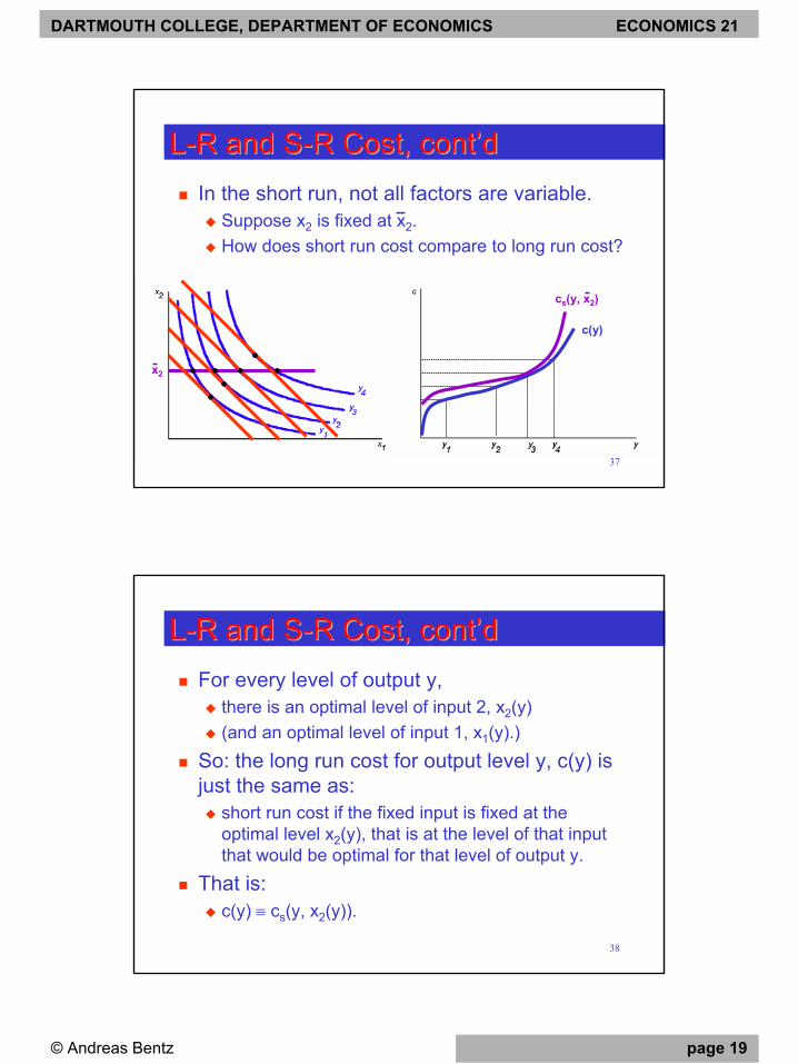
LL--R and SR and S--R Cost, cont’dR Cost, cont’d

x2

c(y)

cs(y, x2)

In the short run, not all factors are variable.Suppose x2 is fixed at x2.How does short run cost compare to long run cost?

38

LL--R and SR and S--R Cost, cont’dR Cost, cont’dFor every level of output y,

there is an optimal level of input 2, x2(y)(and an optimal level of input 1, x1(y).)

So: the long run cost for output level y, c(y) is just the same as:

short run cost if the fixed input is fixed at the optimal level x2(y), that is at the level of that input that would be optimal for that level of output y.

That is:c(y) ≡ cs(y, x2(y)).



39

LL--R and SR and S--R Cost, cont’dR Cost, cont’dIn the diagram on slide 37, the optimal level of input 2 for an output level of y3 would have been x2.

Therefore, when in the short run input 2 was fixed at x2, the short run cost function for output y3 was the same as the long run cost function for output y3.But for all other output levels, the short run cost was higher than the long run cost, because input 2 was fixed at the “wrong” level.

40

(Short Run) Marginal Cost(Short Run) Marginal CostThe short run total cost function is: cs(y, x2).Marginal cost is the rate at which short run cost increases as output is increased. So:

y)x,y(c)y(MC 2s

∂∂

=

y

cs cs(y, x2)

y

MCMC



41

(Short Run) Marginal Cost, cont’d(Short Run) Marginal Cost, cont’dThere is a close connection between long run marginal cost and (short run) marginal cost:

Remember that: c(y) ≡ cs(y, x2(y)).

y

cscs(y, x2*)

y

MCMC

c(y)

LMC

y* y*

42

(Short Run) Marginal Cost, cont’d(Short Run) Marginal Cost, cont’dRemember that: c(y) ≡ cs(y, x2(y)).

Differentiate both sides with respect to y to obtain:

dy)y(dx

x)x,y(c 2

2

2s

∂∂

+y

)x,y(c 2s

∂∂

dy)y(dc =

LMC = MC + stuffWe want to know what LMC is at the output level y* for which x2* is just the right level of input 2:

∂cs(y*, x2*) / ∂x2 = 0 when x2 is chosen optimally (i.e. such that it minimizes cost), so at that point:

y*)x*,y(c

dy*)y(dc 2s

∂∂

=



43

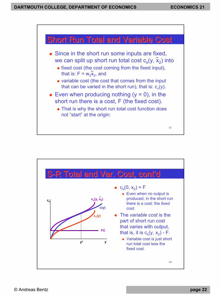
Short Run Total and Variable CostShort Run Total and Variable CostSince in the short run some inputs are fixed, we can split up short run total cost cs(y, x2) into

fixed cost (the cost coming from the fixed input), that is: F = w2x2, andvariable cost (the cost that comes from the input that can be varied in the short run), that is: cv(y).

Even when producing nothing (y = 0), in the short run there is a cost, F (the fixed cost).

That is why the short run total cost function does not “start” at the origin:

44

SS--R Total and Var. Cost, cont’dR Total and Var. Cost, cont’dcs(0, x2) = F

Even when no output is produced, in the short run there is a cost: the fixed cost.

The variable cost is the part of short run cost that varies with output, that is, it is cs(y, x2) - F.

Variable cost is just short run total cost less the fixed cost.

y

cscs(y, x2)

c(y)

y*

FC

cv(y)



45

SS--R Average CostR Average CostAverage Fixed Cost:

AFC = F / yAverage Variable Cost:

AVC = cv(y) / yAverage Total Cost

ATC = cs(y, x2) / y, or:

cs(y, x2) = cv(y) + Fcs(y, x2)/y = cv(y)/y + F/yATC = AVC + AFCy

c

AFC

AVC

ATC

MC

Marginal Cost intersects AVC and ATC at their minimum points.

46

Buzz Group: CostBuzz Group: CostIf the short run total cost curve is: cs(y, 2) = 5 y2 + 20

What is Average Total Cost?» ATC(y) =

What is Fixed Cost?» F =

What is Variable Cost?» VC(y) =

What is Average Variable Cost?» AVC(y) =

What is Marginal Cost?» MC(y) =



47

Short Run Average Total CostShort Run Average Total CostRemember that:

c(y*) ≡ cs(y*, x2*), and c(y) ≤ cs(y, x2).So we have the following relationship between (short run) average total cost and (long run) average cost:

AC(y*) = c(y*) / y* = cs(y*, x2*) / y* = ATC(y*)AC(y) = c(y) / y ≤ cs(y, x2) / y = ATC(y)

That is:Short run ATC is always above long run AC ...and the two are equal at the output level where short run cost = long run cost (which is also the output level at which marginal costs are equal).

48

SS--R Average Total Cost, cont’dR Average Total Cost, cont’d

Short run ATC is always above long run AC ...… and the two are equal at the output level where short run cost = long run cost



49

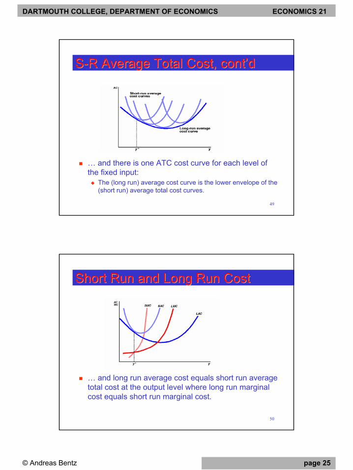
SS--R Average Total Cost, cont’dR Average Total Cost, cont’d

… and there is one ATC cost curve for each level of the fixed input:

The (long run) average cost curve is the lower envelope of the (short run) average total cost curves.

50

Short Run and Long Run CostShort Run and Long Run Cost

… and long run average cost equals short run average total cost at the output level where long run marginal cost equals short run marginal cost.



51

Returns to Scale: Returns to Scale: ConstConst. Returns. Returns


Firm Decisions IIIFirm Decisions III

Profit Maximization again



53

SupplySupplyA firm aims to supply the quantity of output that maximizes its profit:

maxy revenue - costfor each perfectly competitive firm:

competitive firms are “price takers”: they face a horizontal demand curve:maxy p • y - cs(y, x2)

for a monopolist:a monopolist faces the (inverse) market demand curve p(y):maxy p(y) • y - cs(y, x2)


Firm Decisions:Firm Decisions:Competitive FirmsCompetitive Firms

ex pluribus unum



55

Supply: Competitive FirmSupply: Competitive FirmA perfectly competitive firm’s problem is to:

maxy p • y - cs(y, x2)The necessary (first-order) condition for maximization is:

p - ∂cs(y, x2)/∂y = 0∂cs(y, x2)/∂y = pMC(y) = p(but only when it’s better to produce in the short run than to shut down, that is when:

» p • y - cs(y, x2) > - F» p • y - VC(y) - F > - F» p > VC(y)/y, or: p > AVC(y).)

56

Supply: Competitive Firm, cont’dSupply: Competitive Firm, cont’d

A competitive firm’s supply curve is its marginal cost curve above AVC.



57

Buzz Group: Competitive FirmBuzz Group: Competitive FirmIf the short run total cost curve is: cs(y, 2) = 5 y2 + 20What is the firm’s profit? At what output is it maximized?

π(y) = p y - (5 y2 + 20)π’(y) = p - 10 yprofit maximum: π’(y) = 0, or: p = 10 y, or: y = p/10

If the firm produces that output, what is its (maximum) profit?

p (p/10) - (5 • (p/10)2 + 20) = p2/20 - 20

58

Supply: Competitive Firm, cont’dSupply: Competitive Firm, cont’dIn competitive markets, there is free entry into, and exit from, the market.

If firms in this market make positive profits, there is an incentive for other firms to enter the market …… which lowers price …… and erodes profits.

When is there no opportunity for firms to make positive profits (i.e. when will entry no longer occur)?

When π(y) = p y - cs(y, x2) = 0, and no other choice of x2 can give you lower cost.That is, when p = cs(y, x2) / y ≡ ATC(y), and you are operating on the lowest possible ATC curve.That is, when you are operating at the lowest point on LAC.



59

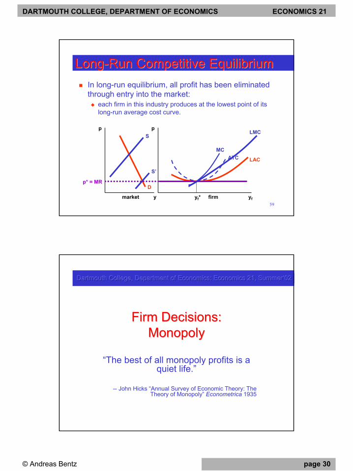
LongLong--Run Competitive EquilibriumRun Competitive EquilibriumIn long-run equilibrium, all profit has been eliminated through entry into the market:

each firm in this industry produces at the lowest point of its long-run average cost curve.

y

p

yf

p

D

S

market firm

LAC

LMC

yf*

S’

p* = MR

MCATC


Firm Decisions:Firm Decisions:MonopolyMonopoly

“The best of all monopoly profits is a quiet life.”

-- John Hicks “Annual Survey of Economic Theory: The Theory of Monopoly” Econometrica 1935



61

Supply: MonopolistSupply: MonopolistA monopolist’s problem is to:

maxy p(y) • y - cs(y, x2)The necessary (first-order) condition for maximization is:

dp(y)/dy • y + p(y) - ∂cs(y, x2)/∂y = 0∂cs(y, x2)/∂y = p(y) [1 + dp(y)/dy • y/p(y)]MC(y) = p(y) [1 + 1/η] ≡ MR(y)

Mark-up pricing:p(y) = [1/(1+1/η)] • MC(y)

62

Supply: Monopolist, cont’dSupply: Monopolist, cont’dExample:

linear (inverse) demand p(y) = a - byπ(y) = (a - by) • y - cs(y, x2) = ay - by2 - cs(y, x2)

» ay - by2 is revenueπ’(y) = a - 2by - ∂cs(y, x2)/∂y

» a - 2by is marginal revenueprofit maximum: a - 2by = MC(y)



63

Supply: Monopolist, cont’dSupply: Monopolist, cont’d

Linear demand p(y) = a - by, so MR(y) = a - 2by


Market Structure IMarket Structure I

Monopoly Behavior:Price Discrimination and

Two-Part Tariffs



65

Price DiscriminationPrice DiscriminationFirst-degree (perfect) price discrimination:

different prices for different units of output, anddifferent prices for different consumers.

Second-degree price discrimination (non-linear pricing):

different prices for different units of output, andsame prices for similar customers.

Third-degree price discrimination:same prices for different units of output, butdifferent prices for different customers.

66

FirstFirst--Degree Price DiscriminationDegree Price Discrimination

The perfectly discriminating monopolist knows each consumer’s demand curve.The monopolist prices each unit of output at each consumer’s marginal willingness to pay.



67

FirstFirst--Degree Price Disc., cont’dDegree Price Disc., cont’d

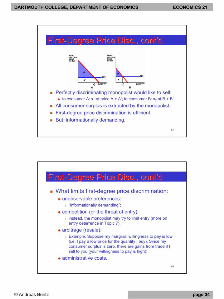
Perfectly discriminating monopolist would like to sell:to consumer A: x1 at price A + A’; to consumer B: x2 at B + B’

All consumer surplus is extracted by the monopolist.First-degree price discrimination is efficient.But: informationally demanding.

68

FirstFirst--Degree Price Disc., cont’dDegree Price Disc., cont’dWhat limits first-degree price discrimination:

unobservable preferences:» “informationally demanding”;

competition (or the threat of entry):» instead, the monopolist may try to limit entry (more on

entry deterrence in Topic 7);arbitrage (resale):

» Example: Suppose my marginal willingness to pay is low (i.e. I pay a low price for the quantity I buy). Since my consumer surplus is zero, there are gains from trade if I sell to you (your willingness to pay is high);

administrative costs.



69

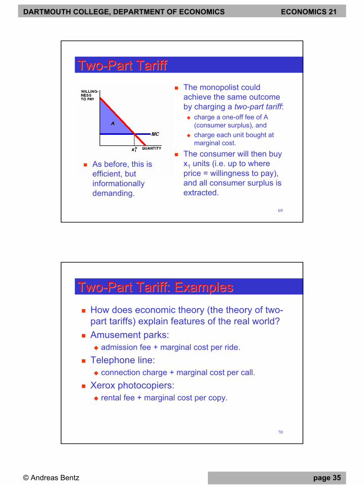
TwoTwo--Part TariffPart TariffThe monopolist could achieve the same outcome by charging a two-part tariff:

charge a one-off fee of A (consumer surplus), andcharge each unit bought at marginal cost.

The consumer will then buy x1 units (i.e. up to where price = willingness to pay), and all consumer surplus is extracted.

As before, this is efficient, but informationally demanding.

70

TwoTwo--Part Tariff: ExamplesPart Tariff: ExamplesHow does economic theory (the theory of two-part tariffs) explain features of the real world?Amusement parks:

admission fee + marginal cost per ride.Telephone line:

connection charge + marginal cost per call.Xerox photocopiers:

rental fee + marginal cost per copy.



71

SecondSecond--Degree Price Disc.Degree Price Disc.Suppose a monopolist cannot observe each customer’s marginal willingness to pay.

But: she can observe the quantity demanded by customers.She could sell different price-quantity “packages”, aimed at customers with different marginal willingness to pay: customers will self-select into buying the “package” designed for them.

An example of an asymmetric information problem (more in Topic 5).

72

ThirdThird--Degree Price DiscriminationDegree Price DiscriminationThe monopolist charges different prices to different customers (i.e. in different elasticity markets).

Examples: private/business telephony, student discounts, business/economy class air travel, …(The monopolist must be able to observe a customer’s demand elasticity.)

Marginal cost equals marginal revenue in each market. (Monopoly pricing in each market.)

(argument by contradiction)



73

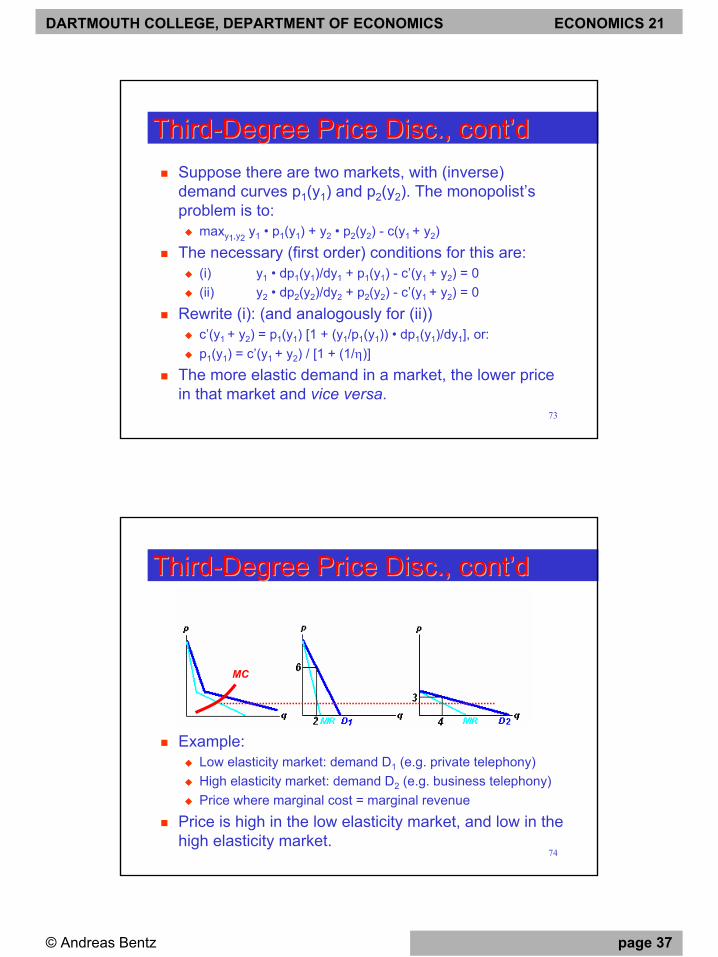
ThirdThird--Degree Price Disc., cont’dDegree Price Disc., cont’dSuppose there are two markets, with (inverse) demand curves p1(y1) and p2(y2). The monopolist’s problem is to:

maxy1,y2 y1 • p1(y1) + y2 • p2(y2) - c(y1 + y2)The necessary (first order) conditions for this are:

(i) y1 • dp1(y1)/dy1 + p1(y1) - c’(y1 + y2) = 0(ii) y2 • dp2(y2)/dy2 + p2(y2) - c’(y1 + y2) = 0

Rewrite (i): (and analogously for (ii))c’(y1 + y2) = p1(y1) [1 + (y1/p1(y1)) • dp1(y1)/dy1], or:p1(y1) = c’(y1 + y2) / [1 + (1/η)]

The more elastic demand in a market, the lower price in that market and vice versa.

74

ThirdThird--Degree Price Disc., cont’dDegree Price Disc., cont’d

Example:Low elasticity market: demand D1 (e.g. private telephony)High elasticity market: demand D2 (e.g. business telephony)Price where marginal cost = marginal revenue

Price is high in the low elasticity market, and low in the high elasticity market.

MC



75

ThirdThird--Degree Price Disc.: WelfareDegree Price Disc.: WelfareThe welfare effects of third-degree price discrimination (compared with standard monopoly pricing) are ambiguous:Two inefficiencies:

Output is too low:» The monopolist charges the monopoly price in each market.

(She restricts output below the efficient level.)Misallocation of goods:

» Goods are allocated to the wrong individuals.» Example: I value a theater ticket at $20, you value it at $10. You

get a student discount (ticket for $8) and buy the ticket. I have to pay the normal price ($28) so I don’t buy the ticket. But my valuation is higher than yours!

And a welfare improvement over monopoly: ...

76

ThirdThird--Degree Price Disc.: WelfareDegree Price Disc.: Welfare

If the monopolist were not allowed to (third-degree) price-discriminate, she might only sell in one market:

Pricing uniformly in both markets may be less profitable than selling in only one market.In this example, the monopolist would only sell in market 1: profit in market 1 is greater than profit in market 2

MC




Market Structure IIMarket Structure II

Monopolistic Competition:Differentiated Products and the

Hotelling Model

78

Product DifferentiationProduct DifferentiationMonopolistic Competition: every firm faces a downward-sloping demand curve (i.e. has some degree of monopoly power).In an industry with non-homogeneous products, how do firms choose their products’ characteristics?

Example: cars, economics courses, …Imagine one product characteristic that can be chosen continuously: e.g. location of two ice-cream vendors along a beachfront.



79

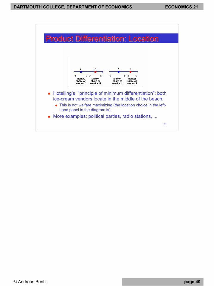
Product Differentiation: LocationProduct Differentiation: Location

Hotelling’s “principle of minimum differentiation”: both ice-cream vendors locate in the middle of the beach.

This is not welfare maximizing (the location choice in the left-hand panel in the diagram is).

More examples: political parties, radio stations, ...

Documents

S-2 -Theory of the Firm - Dartmouth Collegeecon21/x02-topic2.pdfTopic 2: Theory of the Firm Economics 21, Summer 2002 Andreas Bentz Based Primarily on Varian, Ch. 18-25 2 The Setup