Embed Size (px)
DESCRIPTION
mechanics
Citation preview
Date:
Experiment - 1
Basics of Structures
Aim : To study various civil engineering structures and general structural
understanding and how to find structural degrees of indeterminacy.
Theory : i) Basic understanding of structures
An important consideration in engineering design is the capacity of the
object being designed to support or transmit loads. Objects that must sustain
loads include building structures, machines, aircrafts, vehicles, ships and
seemingly endless list of other man-made things. For simplicity, we will
refer to all such objects as structures; thus, a structure is any object that must
support or transmit loads. In other word a structure is an arrangement of
structural elements to receive and transfer safely the load to the subsoil.
If structural failure is to be avoided, the loads that a structure actually can
support must be greater than the loads it will required to sustain when in
service. The ability of a structure to resist loads is called strength.
A detailed study of structures, including their design for safe working
condition is known as “Theory of Structures”. Actually structural analysis is
an integral part of structural design, involves the determination of forces
developed in various components of the structure for the given loading.
A structural element subjected to loads or forces is termed as body. Body
may be rigid or elastic (deformable) in nature.
Elastic body- A body is said to be perfectly elastic if deformation produced
due to application of external force completely disappears after the removal
of the load. In other word deformable bodies are those whose shape and
volume change under the action of forces.
Rigid body- A body is said to be rigid when distance between two points
remains always the same for any arbitrary chosen points of the body under
loading. Actually, solid bodies are never rigid; the deform under the action
of applied forces. In many cases, this deformation is negligible compared to
the size of the body and the body may be assumed rigid. The study of
strength of materials is based on the deformation of elastic bodies. Whereas
the study of engineering mechanics is entirely based on the rigid bodies.
If the body traces back the original path of deflection on removal of load is
termed as a linearly elastic body.
ii) Classification of structures- structures can be classified in several ways,
depending upon the parameters involved. These parameters include
structural action, structural configuration, type of structural systems, types of
joints, type of applied loading and material of the structure.
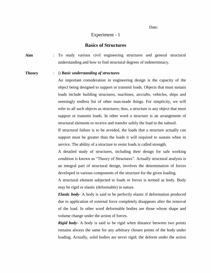
1. On the basis of structural action : Basically there are two types of
structural elements – those subjected to axial forces (A.F) and others
subjected to moments. Axial forces can be tensile or compressive,
and moment can be bending or torsion. A combination of these
structural actions is possible in complex structures.
P P1 P2
Bending
P
P
Axial Compression Axial Tension P Torsion
2. On the basis of structural geometry : Structural geometry can vary
over a wide spectrum, and can include one, two and three
dimensional forms. The structure may comprises
a. Linear elements (1D) (Skeletal structures)
The two dimensions are negligible as compared with first one.
Like frames and trusses.
b. Planar elements (2D) (Surface structures)
One of the three dimensions is negligible compared to others.
Examples are plates, shells and walls.
c. Solid elements (3D) (Solid structures)
All the 3 dimensions i.e. length, breadth and height are
comparable. e.g. dams, tunnels etc.
d. Curved elements like arches and shells.
3. On the basis of joints:
a. Pin jointed structure – examples are Trusses, hinges of doors &
windows etc.
b. Rigid jointed structure – examples are Angle structures, fixed
end, Welded structures, buildings etc.
Each one of these are further classified as-
Plane frames & Space frame.
Plane frames- All the structural members and forces lie on one
plane.
Space frames- any one of the structural members or forces do not
lie in the same plane as others.
4. On the basis of structural systems: structures can be grouped as
statically determinate or statically indeterminate depending upon the
complexity of the analysis involved. The former type can be
analyzed by applying simply the principles of equilibrium of forces,
whereas the latter require more complex techniques involving the
displacement conditions in addition to the equilibrium conditions.
Further, forces or displacements can form the basis of analysis for
statically or kinematically structures.
5. On the basis of applied loading :
a) Structure subjected to static load
b) Structure subjected to dynamic load
c) Structure subjected to impact load.
6. On the basis of materials : Like R.C.C structure, Steel Structure,
Wooden structure, Masonry structures etc.
iii) Force system :
Force- it is defined as an external agent which produces or tends to
produce a change in a body‟s state of rest or of uniform motion . force
system i.e. combination of different forces acting in different directions &
can be classified as :
Concurrent forces- if the line of action of forces pass through the same
point.
Non – concurrent forces- if the lines of actions of the forces do not pass
through the same point.
Coplanar forces- if the forces lie in the same plane.
Non –coplanar forces: if at least one force does not lie in the same plane.
Concurrent coplanar forces: if the lines of action of forces pass through the
same point and all forces lie in the same plane.
Concurrent non – coplanar forces: if the lines of action of forces pass
through the same point and at least one force does not lie the same plane.
Similarly we can define Non-concurrent coplanar forces & non-concurrent
non-coplanar forces.
iv) Equilibrium:-
It is that state of the body where all the resultant forces acting on the
body is zero. It can be further classified into two types:
1) Static equilibrium: it is that state of the body where all the net forces
acting is zero and the structure is at rest.
2) Dynamic equilibrium: it is that state of the body where the net forces
acting is zero and the structure is in uniform motion i.e. dynamic
state.
3) Free body diagram: the free body diagram is a diagram of a section
of the structure showing all the internal and external forces acting on
that part when isolated. It is drawn to know the internal and external
forces.
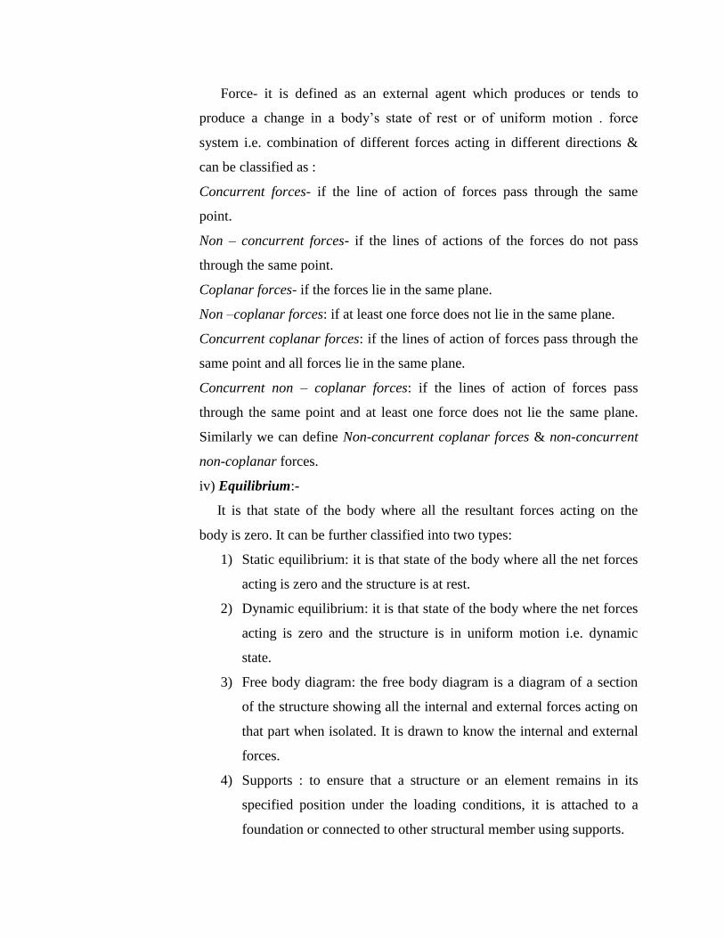
4) Supports : to ensure that a structure or an element remains in its
specified position under the loading conditions, it is attached to a
foundation or connected to other structural member using supports.
e.g. hinged support, roller support and fixed support.
Hinged / Pinned support Roller support
Fixed Support
v) Degree of freedom
A structure may be capable of movements (displacement and rotations) at its
joints and supports after the load are applied. The total numbers of such
possible movements in a structure is known as degree of kinematic
indeterminacy or degrees of freedom.
The pinned support is allows rotation about the defined axes but at the same
time it cannot allow the translation along all the axes.
The roller support is allowed rotation about all the axes and translation along
one define axis whereas other translation are restricted.
The fixed support is not allowed any translation and rotation along and about
the axis respectively.
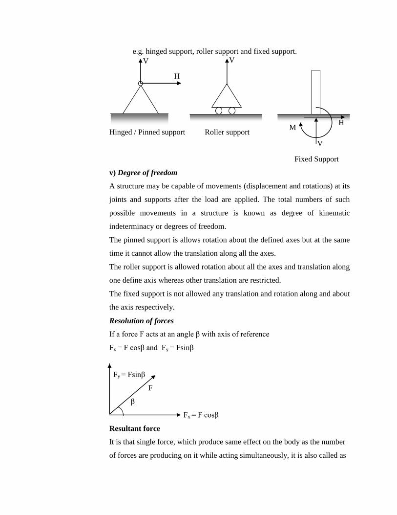
Resolution of forces
If a force F acts at an angle β with axis of reference
Fx = F cosβ and Fy = Fsinβ
Fy = Fsinβ
F
β
Fx = F cosβ
Resultant force
It is that single force, which produce same effect on the body as the number
of forces are producing on it while acting simultaneously, it is also called as
V
H
V
V
H M
equivalent force. Resultant of forces can be found out by graphical method
or analytical method
Compatibility of deformation
In addition to the equilibrium conditions, some the mathematical conditions
are to be included for to solve the unknown quantities of the structure such
additional conditions are called as compatibility of deformation or
compatibility conditions.
For e.g. For a fixed support ∆H=0, ∆V=0 and Ө=0.
In general structures are of following two types
1. Statically determinate structures
2. Statically indeterminate structures
Statically determinate structures
Statically indeterminate
structures
Conditions of equilibrium are
sufficient to fully analyze the
structure
Conditions of equilibrium are
not sufficient.
B.M at a section and the force
in any member is independent
of material of the components
of structure.
They are not independent
No stress are caused due to
temporary changes
Stress are generated due to
temporary changes.
On the basis of alignment of forces, support and members structures are
classified as
Plane frame: in which all members and forces are in the same plane.
Space frames: in which at least one member is out of plane.
On the basis of the type of support, structure are classified as pin jointed and
rigid jointed.
iii) Degree of indeterminacy
It is the number of additional equations required besides the equations of
equilibrium to determine all the external and internal reactions and moments.
It is also called the degree of redundancy.
Statically indeterminacy:
It is stated in terms of external indeterminacy and internal indeterminacy.
External indeterminacy.
When the three equations of equilibrium are insufficient to determine all the
reactions at the supports. It is given by number of unknown reactions at
support minus number of known equations of equilibrium.
Internal indeterminacy.
A structure is said to be statically indeterminate if it is a closed structure. So
the minimum cuts are required to open all close loops gives the internal
indeterminacy.
Kinematic indeterminacy: A structure is said to be statically kinematically
Indeterminate if its deformation cannot be determined completely using the
support condition.
For pin jointed structures:
Internal indeterminacy:
A plane frame pin jointed structure is said to be a perfect or statically
internally determinate if
M = 2j – 3
Where,
M – no. of structural members in frame
j - no. of joints in the frame
For a space frame, pin jointed structure is said to be determinate one if,
M = 3j – 6
The excess no. of members adds to the degree of redundancy.
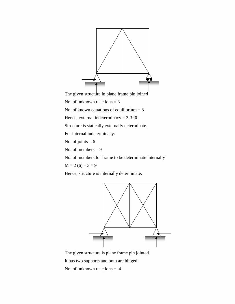
i) The given structure in plane frame pin joined
No. of unknown reactions = 3
No. of known equations of equilibrium = 3
Hence, external indeterminacy = 3-3=0
Structure is statically externally determinate.
For internal indeterminacy:
No. of joints = 6
No. of members = 9
No. of members for frame to be determinate internally
M = 2 (6) – 3 = 9
Hence, structure is internally determinate.
ii) The given structure is plane frame pin jointed
It has two supports and both are hinged
No. of unknown reactions = 4
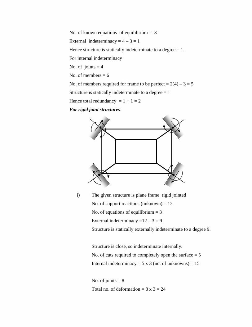
No. of known equations of equilibrium = 3
External indeterminacy = 4 – 3 = 1
Hence structure is statically indeterminate to a degree = 1.
For internal indeterminacy
No. of joints = 4
No. of members = 6
No. of members required for frame to be perfect = 2(4) – 3 = 5
Structure is statically indeterminate to a degree = 1
Hence total redundancy = 1 + 1 = 2
For rigid joint structures:
i) The given structure is plane frame rigid jointed
No. of support reactions (unknown) = 12
No. of equations of equilibrium = 3
External indeterminacy =12 – 3 = 9
Structure is statically externally indeterminate to a degree 9.
Structure is close, so indeterminate internally.
No. of cuts required to completely open the surface = 5
Internal indeterminacy = 5 x 3 (no. of unknowns) = 15
No. of joints = 8
Total no. of deformation = 8 x 3 = 24
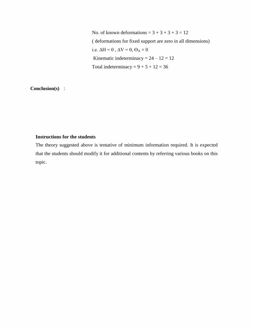
No. of known deformations = 3 + 3 + 3 + 3 = 12
( deformations for fixed support are zero in all dimensions)
i.e. ∆H = 0 , ∆V = 0, ӨA = 0
Kinematic indeterminacy = 24 – 12 = 12
Total indeterminacy = 9 + 5 + 12 = 36
Conclusion(s) :
Instructions for the students
The theory suggested above is tentative of minimum information required. It is expected
that the students should modify it for additional contents by referring various books on this
topic.
Date:
Experiment - 2
Verification of Shear Force and Bending Moment Diagrams
for Beams using Standard Structural Analysis Package
Aim : To determine the shear force and bending moment diagrams for different
structures manually and verifying it using SAP2000 NL software
Theory : The term beam refers to a slender bar that carries transverse loading; that
is, the applied forces are perpendicular to the bar. In a beam, the internal
force system consists of a shear force and bending moment acting on the
cross section of the bar. The internal forces give rise to two kinds of
stresses on a transverse section of a beam: 1) Normal stress that is caused
by the bending moment and 2) shear stress due to the shear force.
The determination of the internal force system acting at a given section
of a beam is straightforward: We draw a free-body diagram that exposes
these forces and then compute the forces using equilibrium equations.
However the goal of beam analysis is to determine the shear force V and
the bending moment M at every cross section of the beam. To
accomplish this task, we must derive the expressions for V and M in
terms of the distance x measured along the beam. By plotting these
expressions to scale, we obtain the shear force and bending moment
diagrams for the beam. The shear force and bending moment diagrams
are convenient visual references to the internal forces in a beam; in
particular, they identify the maximum values of V and M.
When loads are not at right angle to the beam, they also produce axial
forces in the beam.
The transverse loading of a beam consists of concentrated loads,
distributed loads, uniformly distributed loads or a combination of all.
Depending upon the type of support, the reactions at support can be force
or moment. These reactions can be determined by the equations of
equilibrium in case of determinate structures. The bending couple creates
normal stresses while the shear force creates shearing stresses.
Bending moment diagram
The value of bending moment is determined at various points of beam
and plotted against the distance x measured from one end of the beam.
This plotting is known as bending moment diagram.
Sign conventions
Sagging BM is considered +ve
Hogging BM is considered –ve
Shear force diagram
The diagram obtained by plotting values of shear force at various points
of beam and plotted them against x measured from one end of beam is
the shear force diagram.
Sign conventions: if the loads acting on the beam on the right side of the
section deflect it downwards or those at the left side of the section
deflect it upwards then the SF at the section is considered to be +ve.
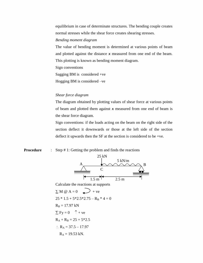
Procedure : Step # 1: Getting the problem and finds the reactions
Calculate the reactions at supports
M @ A = 0 + ve
25 * 1.5 + 5*2.5*2.75 – RB * 4 = 0
RB = 17.97 kN
Fy = 0 + ve
RA + RB = 25 + 5*2.5
RA = 37.5 – 17.97
RA = 19.53 kN.
25 kN 5 kN/m
A B
C
1.5 m 2.5 m
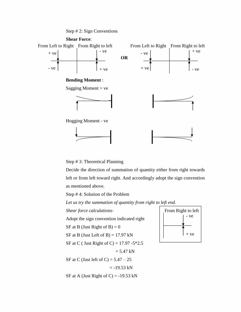
Step # 2: Sign Conventions
Shear Force:
Bending Moment :
Sagging Moment + ve
Hogging Moment - ve
Step # 3: Theoretical Planning
Decide the direction of summation of quantity either from right towards
left or from left toward right. And accordingly adopt the sign convention
as mentioned above.
Step # 4: Solution of the Problem
Let us try the summation of quantity from right to left end.
Shear force calculations-
Adopt the sign convention indicated right
SF at B (Just Right of B) = 0
SF at B (Just Left of B) = 17.97 kN
SF at C ( Just Right of C) = 17.97 -5*2.5
= 5.47 kN
SF at C (Just left of C) = 5.47 – 25
= -19.53 kN
SF at A (Just Right of C) = -19.53 kN
From Left to Right From Right to left
+ ve
- ve
- ve
+ ve
OR
From Left to Right From Right to left
- ve
+ ve
+ ve
- ve
From Right to left - ve
+ ve
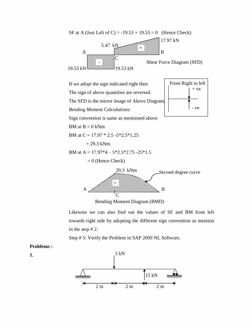
SF at A (Just Left of C) = -19.53 + 19.53 = 0 (Hence Check)
If we adopt the sign indicated right then
The sign of above quantities are reversed.
The SFD is the mirror image of Above Diagram.
Bending Moment Calculations:
Sign convention is same as mentioned above
BM at B = 0 kNm
BM at C = 17.97 * 2.5 -5*2.5*1.25
= 29.3 kNm.
BM at A = 17.97*4 – 5*2.5*2.75 -25*1.5
= 0 (Hence Check)
Likewise we can also find out the values of SF and BM from left
towards right side by adopting the different sign convention as mention
in the step # 2.
Step # 5: Verify the Problem in SAP 2000 NL Software.
Problems :
1.
5 kN
15 kN
2 m 2 m 2 m
From Right to left + ve
- ve
A B
C -
+
17.97 kN 5.47 kN
19.53 kN 19.53 kN
Shear Force Diagram (SFD)
A B
C
29.3 kNm
Bending Moment Diagram (BMD)
+
Second degree curve
2.
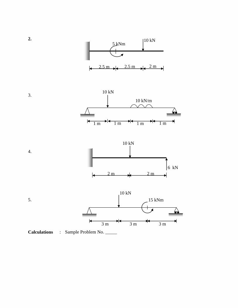
3.
4.
5.
Calculations : Sample Problem No. _____
5 kNm 10 kN
2.5 m 2.5 m 2 m
10 kN
2 m 2 m
6 kN
10 kN
3 m 3 m 3 m
15 kNm
10 kN
1 m 1 m 1 m 1 m
10 kN/m

Instructions for the students
The theory written and sample problems taken above is tentative of minimum information
required. It is expected that the students should modify it for additional contents by
referring various books on this topic. And also the exercise problem may be different for
each student/batch.
Conclusion(s) :
Date:
Experiment -
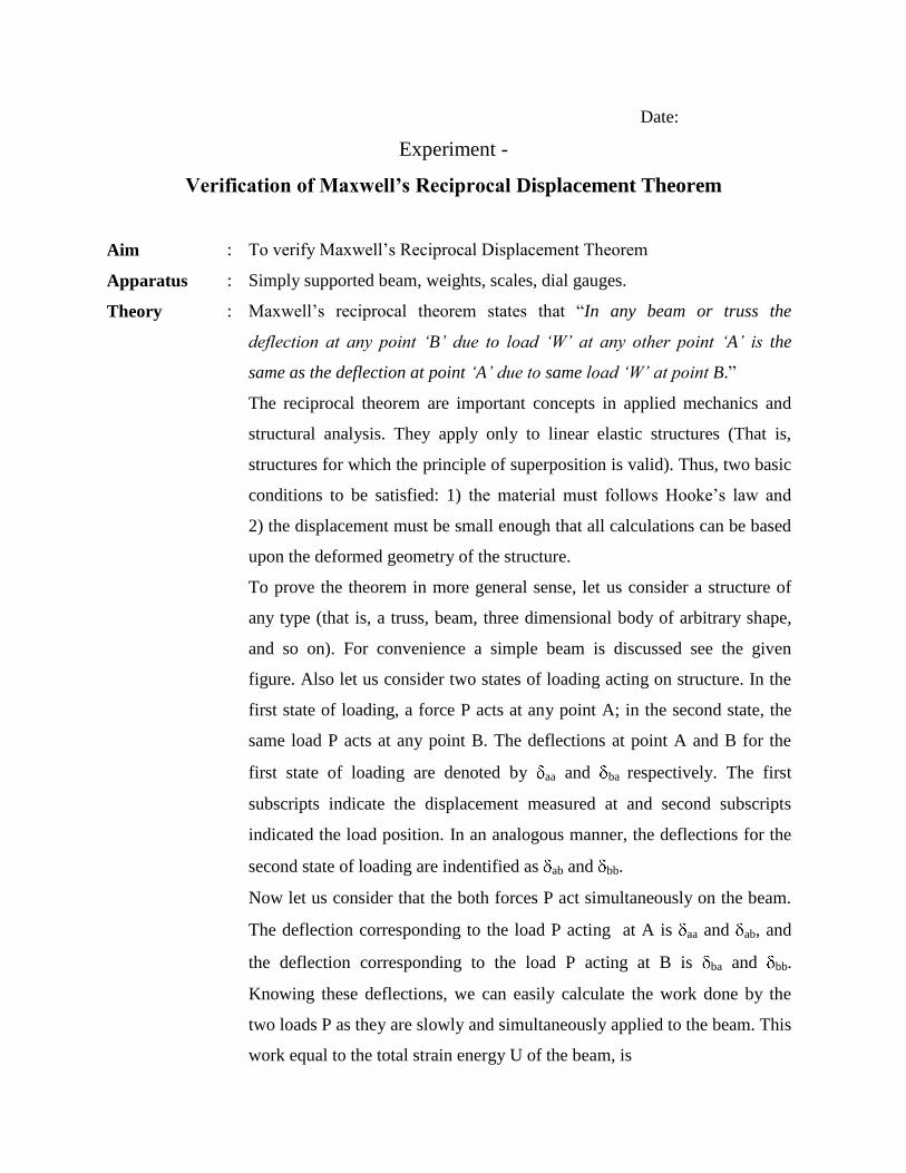
Verification of Maxwell’s Reciprocal Displacement Theorem
Aim : To verify Maxwell‟s Reciprocal Displacement Theorem
Apparatus : Simply supported beam, weights, scales, dial gauges.
Theory : Maxwell‟s reciprocal theorem states that “In any beam or truss the
deflection at any point ‘B’ due to load ‘W’ at any other point ‘A’ is the
same as the deflection at point ‘A’ due to same load ‘W’ at point B.”
The reciprocal theorem are important concepts in applied mechanics and
structural analysis. They apply only to linear elastic structures (That is,
structures for which the principle of superposition is valid). Thus, two basic
conditions to be satisfied: 1) the material must follows Hooke‟s law and
2) the displacement must be small enough that all calculations can be based
upon the deformed geometry of the structure.
To prove the theorem in more general sense, let us consider a structure of
any type (that is, a truss, beam, three dimensional body of arbitrary shape,
and so on). For convenience a simple beam is discussed see the given
figure. Also let us consider two states of loading acting on structure. In the
first state of loading, a force P acts at any point A; in the second state, the
same load P acts at any point B. The deflections at point A and B for the
first state of loading are denoted by aa and ba respectively. The first
subscripts indicate the displacement measured at and second subscripts
indicated the load position. In an analogous manner, the deflections for the
second state of loading are indentified as ab and bb.
Now let us consider that the both forces P act simultaneously on the beam.
The deflection corresponding to the load P acting at A is aa and ab, and
the deflection corresponding to the load P acting at B is ba and bb.
Knowing these deflections, we can easily calculate the work done by the
two loads P as they are slowly and simultaneously applied to the beam. This
work equal to the total strain energy U of the beam, is
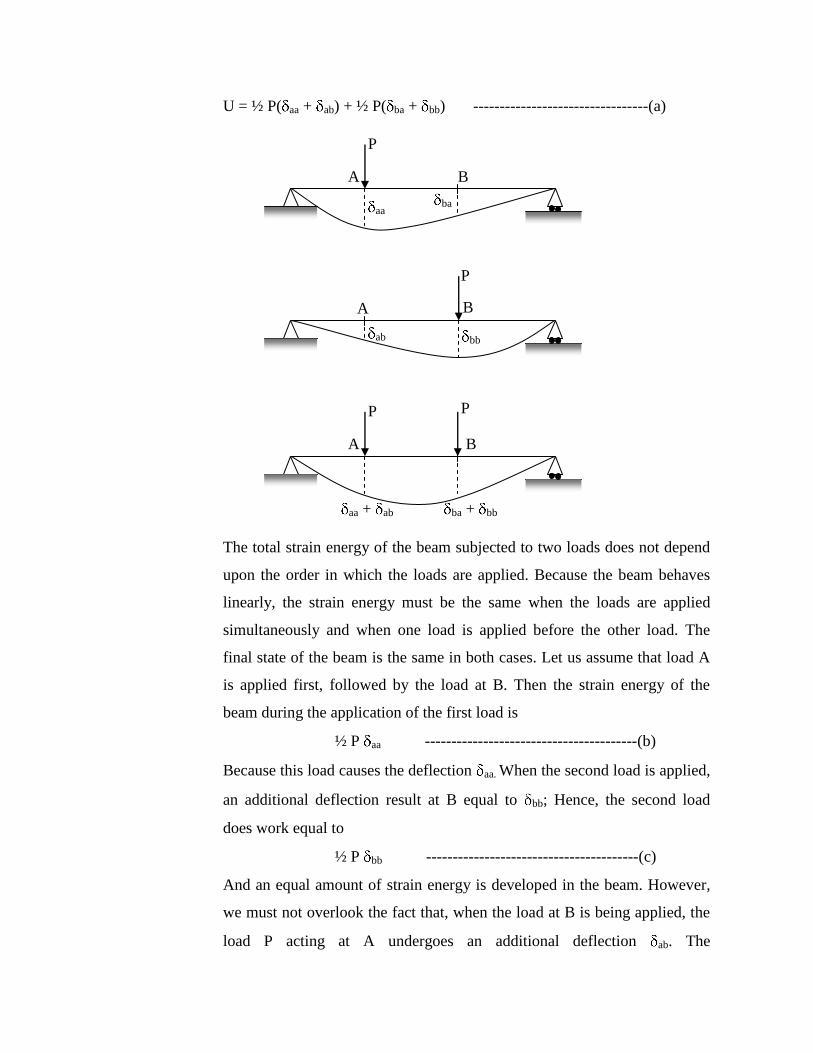
U = ½ P( aa + ab) + ½ P( ba + bb) ---------------------------------(a)
The total strain energy of the beam subjected to two loads does not depend
upon the order in which the loads are applied. Because the beam behaves
linearly, the strain energy must be the same when the loads are applied
simultaneously and when one load is applied before the other load. The
final state of the beam is the same in both cases. Let us assume that load A
is applied first, followed by the load at B. Then the strain energy of the
beam during the application of the first load is
½ P aa ----------------------------------------(b)
Because this load causes the deflection aa. When the second load is applied,
an additional deflection result at B equal to bb; Hence, the second load
does work equal to
½ P bb ----------------------------------------(c)
And an equal amount of strain energy is developed in the beam. However,
we must not overlook the fact that, when the load at B is being applied, the
load P acting at A undergoes an additional deflection ab. The
P
A B
aa ba
P
A B
ab bb
P
A B
aa + ab ba + bb
P
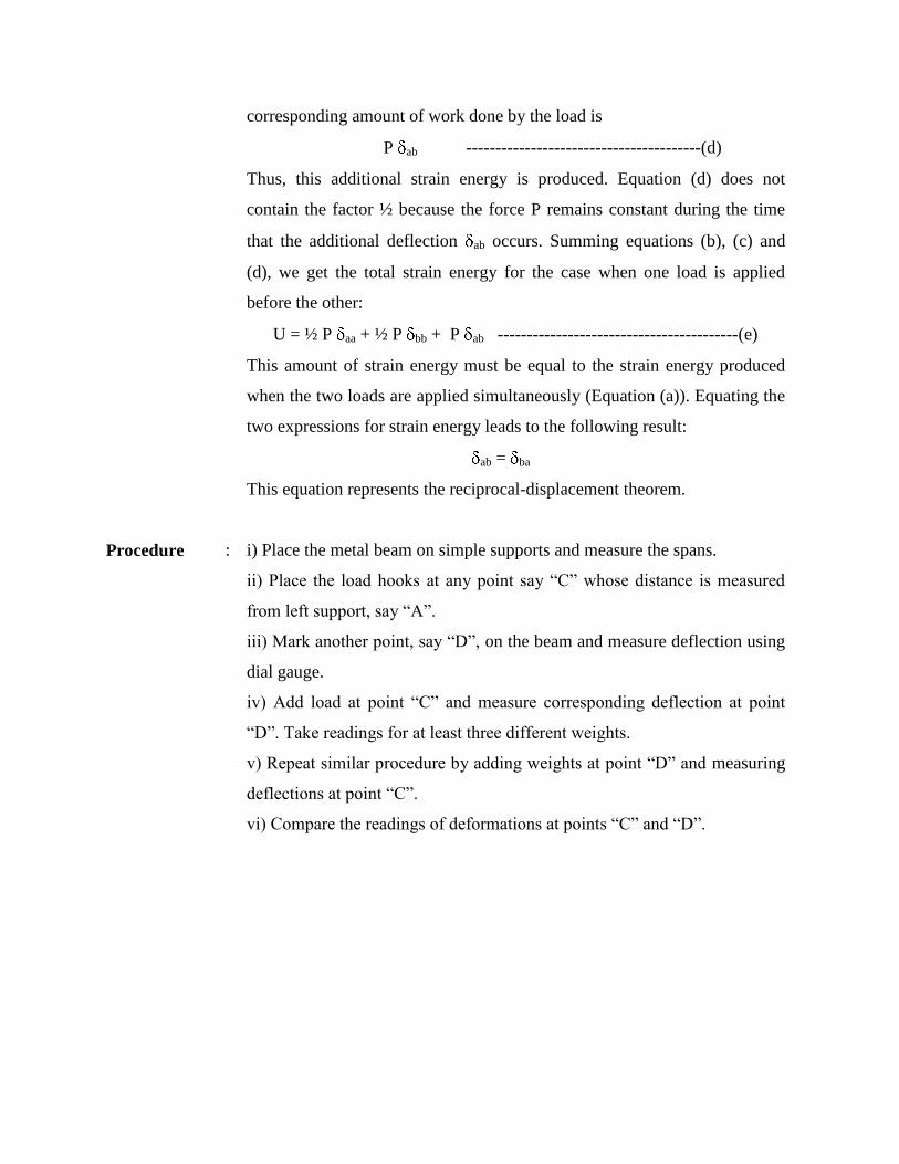
corresponding amount of work done by the load is
P ab ----------------------------------------(d)
Thus, this additional strain energy is produced. Equation (d) does not
contain the factor ½ because the force P remains constant during the time
that the additional deflection ab occurs. Summing equations (b), (c) and
(d), we get the total strain energy for the case when one load is applied
before the other:
U = ½ P aa + ½ P bb + P ab -----------------------------------------(e)
This amount of strain energy must be equal to the strain energy produced
when the two loads are applied simultaneously (Equation (a)). Equating the
two expressions for strain energy leads to the following result:
ab = ba
This equation represents the reciprocal-displacement theorem.
Procedure : i) Place the metal beam on simple supports and measure the spans.
ii) Place the load hooks at any point say “C” whose distance is measured
from left support, say “A”.
iii) Mark another point, say “D”, on the beam and measure deflection using
dial gauge.
iv) Add load at point “C” and measure corresponding deflection at point
“D”. Take readings for at least three different weights.
v) Repeat similar procedure by adding weights at point “D” and measuring
deflections at point “C”.
vi) Compare the readings of deformations at points “C” and “D”.
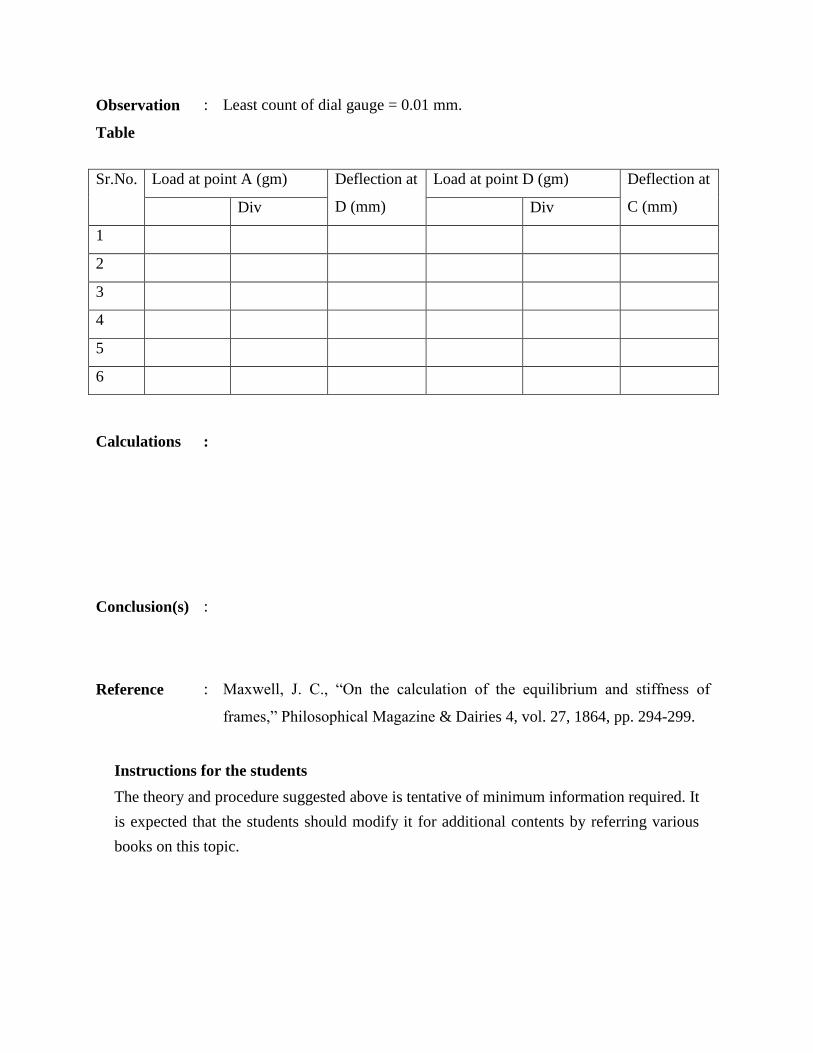
Observation
Table
: Least count of dial gauge = 0.01 mm.
Sr.No. Load at point A (gm) Deflection at
D (mm)
Load at point D (gm) Deflection at
C (mm) Div Div
1
2
3
4
5
6
Calculations
:
Conclusion(s) :
Reference : Maxwell, J. C., “On the calculation of the equilibrium and stiffness of
frames,” Philosophical Magazine & Dairies 4, vol. 27, 1864, pp. 294-299.
Instructions for the students
The theory and procedure suggested above is tentative of minimum information required. It
is expected that the students should modify it for additional contents by referring various
books on this topic.
Experiment No –
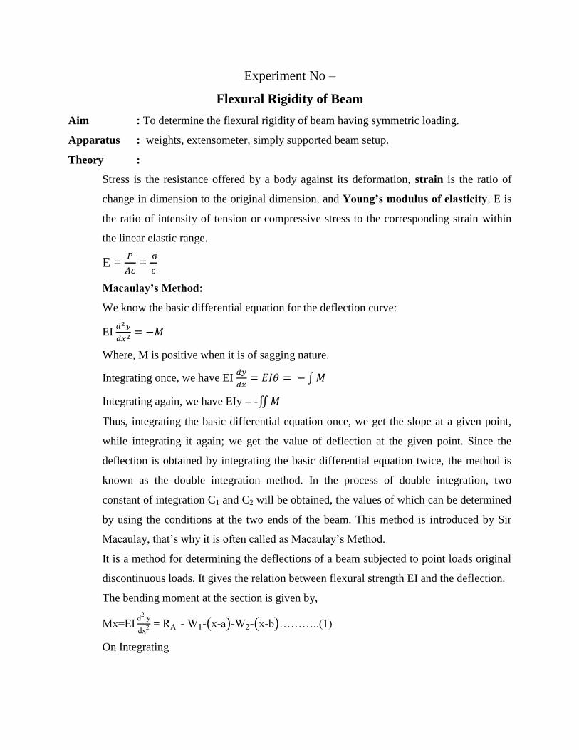
Flexural Rigidity of Beam
Aim : To determine the flexural rigidity of beam having symmetric loading.
Apparatus : weights, extensometer, simply supported beam setup.
Theory :
Stress is the resistance offered by a body against its deformation, strain is the ratio of
change in dimension to the original dimension, and Young’s modulus of elasticity, E is
the ratio of intensity of tension or compressive stress to the corresponding strain within
the linear elastic range.
E = =
Macaulay’s Method:
We know the basic differential equation for the deflection curve:
EI
Where, M is positive when it is of sagging nature.
Integrating once, we have EI
Integrating again, we have EIy = -
Thus, integrating the basic differential equation once, we get the slope at a given point,
while integrating it again; we get the value of deflection at the given point. Since the
deflection is obtained by integrating the basic differential equation twice, the method is
known as the double integration method. In the process of double integration, two
constant of integration C1 and C2 will be obtained, the values of which can be determined
by using the conditions at the two ends of the beam. This method is introduced by Sir
Macaulay, that‟s why it is often called as Macaulay‟s Method.
It is a method for determining the deflections of a beam subjected to point loads original
discontinuous loads. It gives the relation between flexural strength EI and the deflection.
The bending moment at the section is given by,
= - - - - - -
On Integrating
For symmetrically loaded beam,
At = 0
At
Integrating the equation (1),
At y = ymax, putting in equation (3)
Procedure :
Take a simply supported beam and mark point equidistant from the opposite side.
Dial gauge was placed at the centre of the beam to find the deflection.
For different set of symmetric loadings find the deflection.
The observation were made and requisite calculation were performed
Observations :
Span length =
Least count of dial gauge =
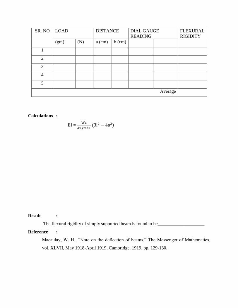
SR. NO LOAD DISTANCE DIAL GAUGE
READING
FLEXURAL
RIGIDITY
(gm) (N)
a (cm) b (cm)
1
2
3
4
5
Average
Calculations :
EI =
Result :
The flexural rigidity of simply supported beam is found to be____________________
Reference :
Macaulay, W. H., “Note on the deflection of beams,” The Messenger of Mathematics,
vol. XLVII, May 1918-April 1919, Cambridge, 1919, pp. 129-130.
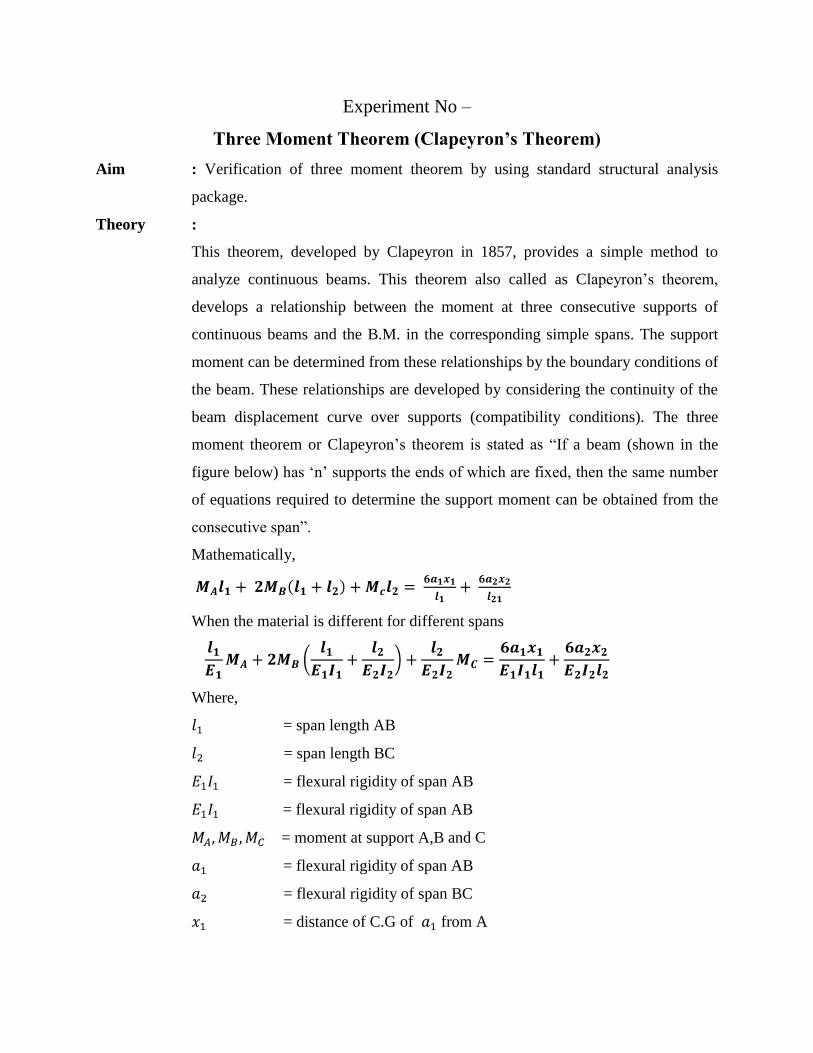
Experiment No –
Three Moment Theorem (Clapeyron’s Theorem)
Aim : Verification of three moment theorem by using standard structural analysis
package.
Theory :
This theorem, developed by Clapeyron in 1857, provides a simple method to
analyze continuous beams. This theorem also called as Clapeyron‟s theorem,
develops a relationship between the moment at three consecutive supports of
continuous beams and the B.M. in the corresponding simple spans. The support
moment can be determined from these relationships by the boundary conditions of
the beam. These relationships are developed by considering the continuity of the
beam displacement curve over supports (compatibility conditions). The three
moment theorem or Clapeyron‟s theorem is stated as “If a beam (shown in the
figure below) has „n‟ supports the ends of which are fixed, then the same number
of equations required to determine the support moment can be obtained from the
consecutive span”.
Mathematically,
When the material is different for different spans
Where,
= span length AB
= span length BC
= flexural rigidity of span AB
= flexural rigidity of span AB
= moment at support A,B and C
= flexural rigidity of span AB
= flexural rigidity of span BC
= distance of C.G of from A
= distance of C.G of from C
Application :
The three hinge moment theorem can be used to analyze beams which are
indeterminate easily. Theory is the most useful in analysis of continuous beams
with simply supports, fixed supports and with overhang.
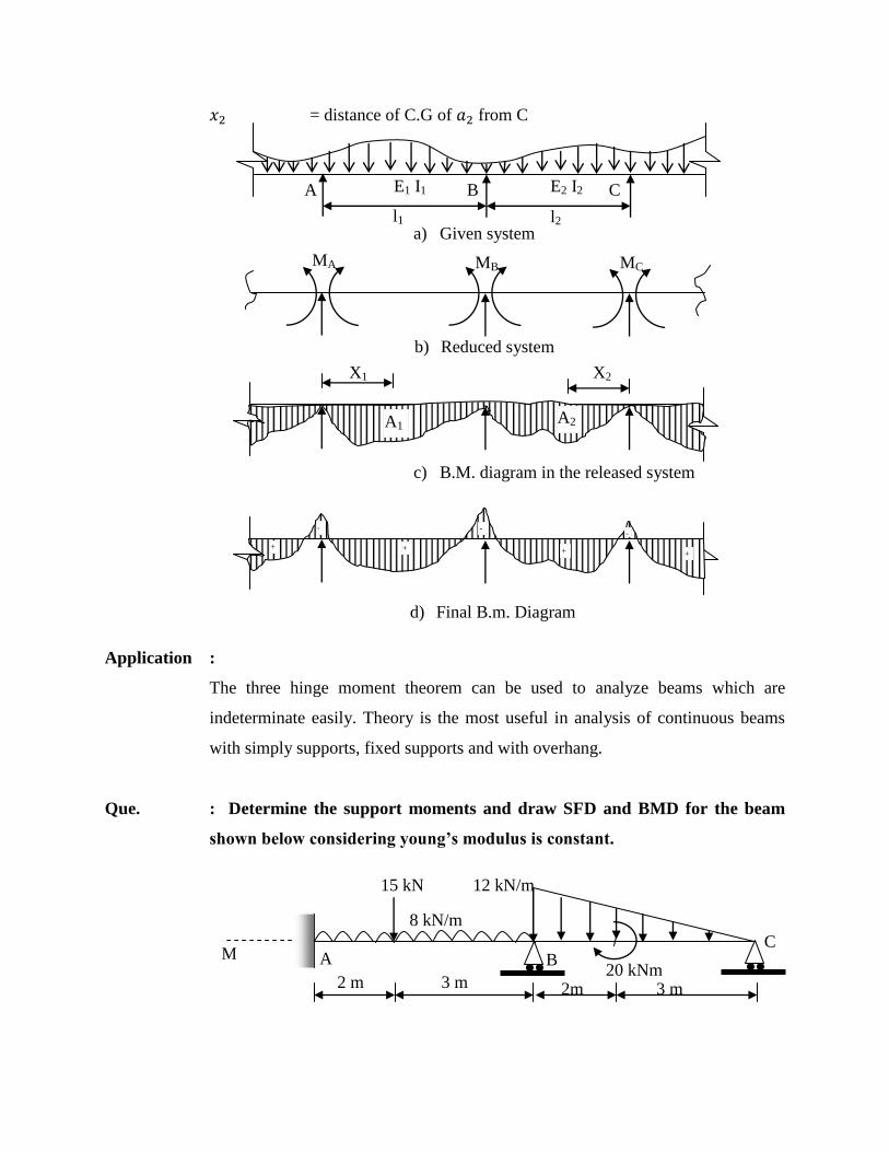
Que. : Determine the support moments and draw SFD and BMD for the beam
shown below considering young’s modulus is constant.
A B C E1 I1 E2 I2
l1 l2
MA MB MC
A1 A2
-
+
-
+ + +
-
X1 X2
a) Given system
b) Reduced system
c) B.M. diagram in the released system
d) Final B.m. Diagram
A B C
15 kN
8 kN/m
12 kN/m
20 kNm 2 m 3 m 3 m 2m
M
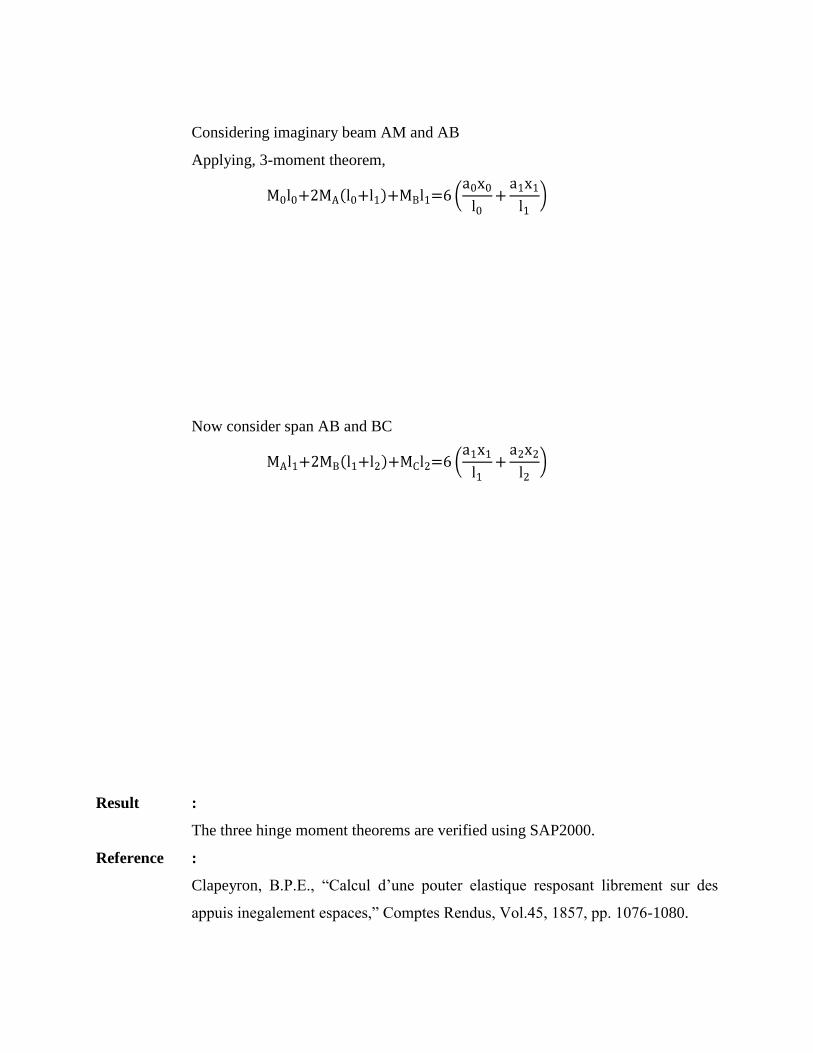
Considering imaginary beam AM and AB
Applying, 3-moment theorem,
Now consider span AB and BC
Result :
The three hinge moment theorems are verified using SAP2000.
Reference :
Clapeyron, B.P.E., “Calcul d‟une pouter elastique resposant librement sur des
appuis inegalement espaces,” Comptes Rendus, Vol.45, 1857, pp. 1076-1080.
Experiment No –
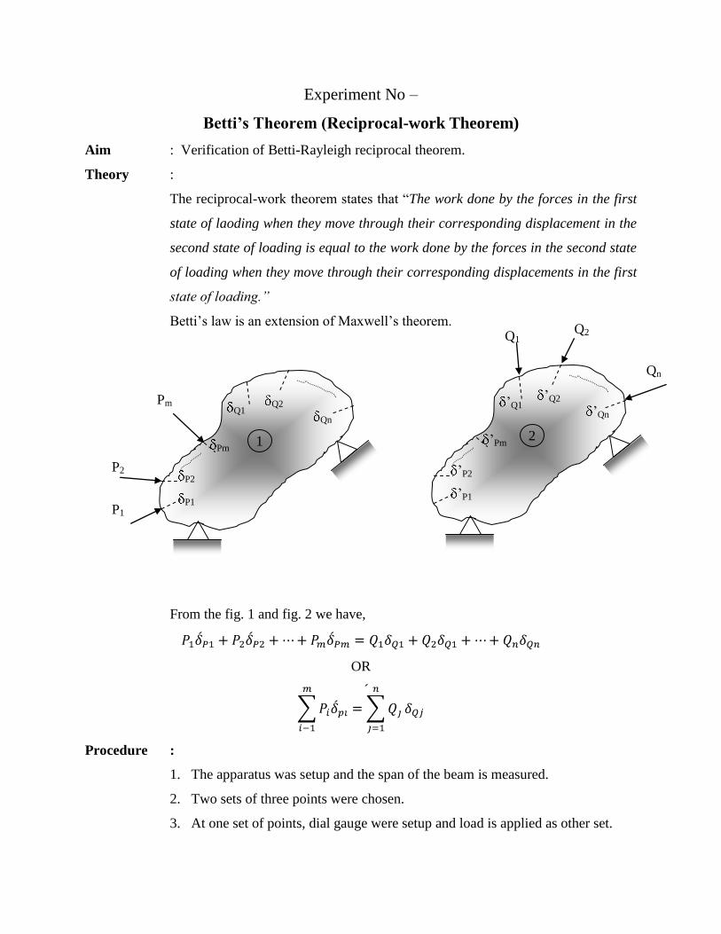
Betti’s Theorem (Reciprocal-work Theorem)
Aim : Verification of Betti-Rayleigh reciprocal theorem.
Theory :
The reciprocal-work theorem states that “The work done by the forces in the first
state of laoding when they move through their corresponding displacement in the
second state of loading is equal to the work done by the forces in the second state
of loading when they move through their corresponding displacements in the first
state of loading.”
Betti‟s law is an extension of Maxwell‟s theorem.
From the fig. 1 and fig. 2 we have,
OR
Procedure :
1. The apparatus was setup and the span of the beam is measured.
2. Two sets of three points were chosen.
3. At one set of points, dial gauge were setup and load is applied as other set.
Pm
P2
P1 P1
P2
Pm
Q1 Q2
Qn
1
‟P1
‟P2
‟Pm
‟Q1 ‟Q2
‟Qn
2
Q1 Q2
Qn
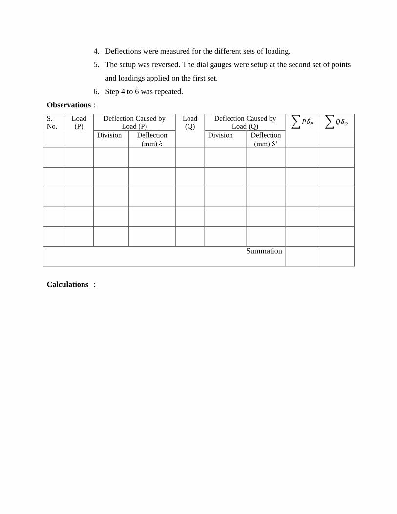
4. Deflections were measured for the different sets of loading.
5. The setup was reversed. The dial gauges were setup at the second set of points
and loadings applied on the first set.
6. Step 4 to 6 was repeated.
Observations :
S.
No.
Load
(P)
Deflection Caused by
Load (P)
Load
(Q)
Deflection Caused by
Load (Q)
Division Deflection
(mm)
Division Deflection
(mm) ‟
Summation
Calculations :
Result :
Reference :
1) Betti, E., “Teoria della Elasticita,” II Nuova Cimento, Series 2, Vol. 7 and 8,
1872.
2) Rayleigh, Lord, “Some General Theorems relating to vibrations,” Proceeding
of London Mathematical Society, Vol. 4, 1873, pp. 357-368.
Date:
Experiment -
Verification of Moment Distribution Method by using Standard Structural
Analysis Software
Aim : Verification of moment distribution method by using some standard structural
analysis software.
Theory : The method of analysis of indeterminate structures involves the formulation and
solution of simultaneous equations. Such process can be tedious, time consuming
and error prone when large structure are analyzed. Thus, methods that did not
involve simultaneous equations were required to analyze large structures before
the advent of computers. Such method was developed early this century which did
not rely exclusive on the solution of simultaneous equations.
The moment distribution method was developed by Prof. Hardy Cross in the
1930s (some time referred as Hardy Cross‟ Method). This method involves the
distributing the known fixed-end moments of the structural members to the
adjacent members of the joints, in order to satisfy the conditions of continuity of
slope and displacements (compatibility conditions). Though this method is
iterative in nature, they converge in a few iterations to the correct solution.
The structural system is first reduced to its kinematically determinate form in this
method. This is accomplished by assuming all the joints to be fully restrained.
The end moments of all the members are computed for this condition of the
structure (all the members having fixed ends). The joints are allow to rotate one
after other by releasing them successively. The unbalanced moment at the joint is
shared by the members connected at the joint when it is released. This method
makes use of the ability of various structural members at a joint to sustain
moments in proportion to their relative stiffnesses. This method provides an
elegant and quick procedure to analyze continuous beams. The method can also
be applied to frames with few additional computations.
Procedure : The process of moment distribution method for prismatic beams is summarized
below:
1. Rotational stiffnesses K of all the members meeting at a joint are computed
depending upon the condition at the far end. The value of K is given by
K = 4EI/L (If the far end is fixed);
K = 3EI/L ( if the far end is simply supported), and
K = 0 (if the far end is free).
2. Distribution factors at each joint are computed on the basis of relative
rotational stiffnesses of the members at that joint. These factors are noted
alone each member meeting at the joint.
3. Fixed end moments (F.E.M) are computed for each member for the given
loading.
4. Moments are released at the simply supported end; these moments are referred
as released moment (R.M). The released moments are carried over to the far
ends of the corresponding members depending upon the carry over factors;
these moments are known as carry over moments (C.O.M.)
5. The unbalanced moments at each joint are computed from the total moments
(T.M) these moments are distributed among the various members meeting at
the joint on the basis of D.F. The unbalanced moments so distributed at a joint
are known as distributed moments (D.M.).
6. The D.M are carried over to the far ends of the corresponding members on the
basis of their C.O.M.
7. Steps 5 and 6 are repeated at each joint until no unbalanced moment exists at
any joint or till the moment carried over is negligible compared to their final
end moments (usually within about one percent)
8. The algebraic sum of all the moments (F.E.M. or T.M., R.M., D.M. and
C.O.M) from all the cycles (Step 5 to 7) for each member meeting at the joint
is calculated. These values are known as the final end moments (F.M.).
Exercise
Problem : Determine the B.M and S.F. diagrams for the beams shown in Fig below.
10 kN/m 50 kN
B C A EI EI
8 m 4 m 2 m
1)
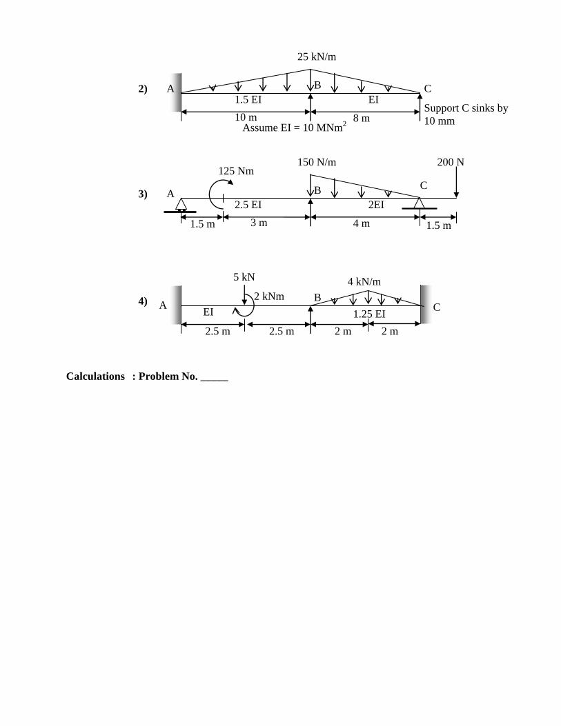
Calculations : Problem No. _____
25 kN/m
B C A 1.5 EI EI
10 m 8 m
2)
Support C sinks by
10 mm Assume EI = 10 MNm
2
150 N/m
B C A
2.5 EI 2EI
3 m 4 m
3)
200 N 125 Nm
1.5 m 1.5 m
4 kN/m
B C A
EI 1.25 EI
2 m
4)
2 m 2.5 m 2.5 m
5 kN
2 kNm
Conclusion :
References : 1. Cross, Hardy (1930), “Analysis of Continuous Frames by Distributing Fixed-
End Moments”. Proceeding of the American Society of Civil Engineers(ASCE):
pp. 919-928.
2. Wang C. K., Indeterminate Structural Analysis, McGraw-Hill Book Co.,
New York (1983).
Date:
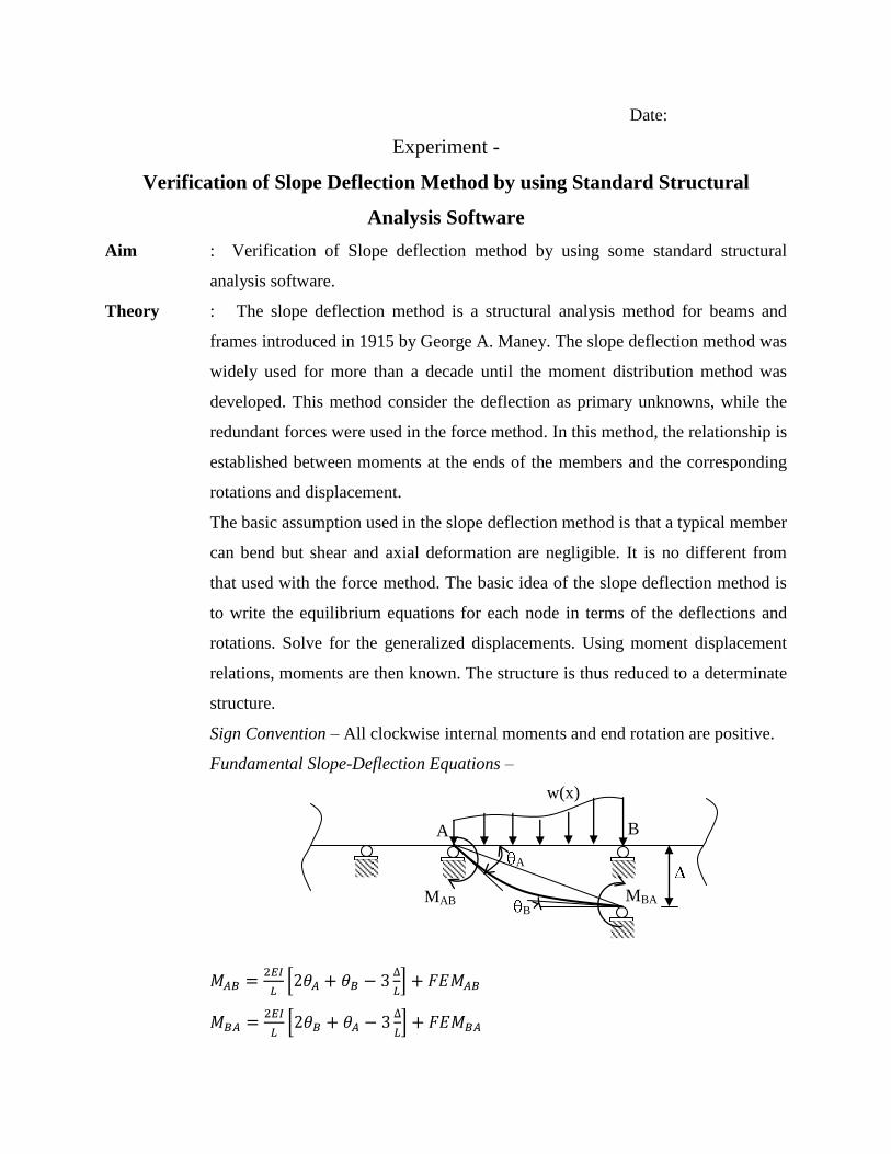
Experiment -
Verification of Slope Deflection Method by using Standard Structural
Analysis Software
Aim : Verification of Slope deflection method by using some standard structural
analysis software.
Theory : The slope deflection method is a structural analysis method for beams and
frames introduced in 1915 by George A. Maney. The slope deflection method was
widely used for more than a decade until the moment distribution method was
developed. This method consider the deflection as primary unknowns, while the
redundant forces were used in the force method. In this method, the relationship is
established between moments at the ends of the members and the corresponding
rotations and displacement.
The basic assumption used in the slope deflection method is that a typical member
can bend but shear and axial deformation are negligible. It is no different from
that used with the force method. The basic idea of the slope deflection method is
to write the equilibrium equations for each node in terms of the deflections and
rotations. Solve for the generalized displacements. Using moment displacement
relations, moments are then known. The structure is thus reduced to a determinate
structure.
Sign Convention – All clockwise internal moments and end rotation are positive.
Fundamental Slope-Deflection Equations –
w(x)
B A
MAB
A
B MBA
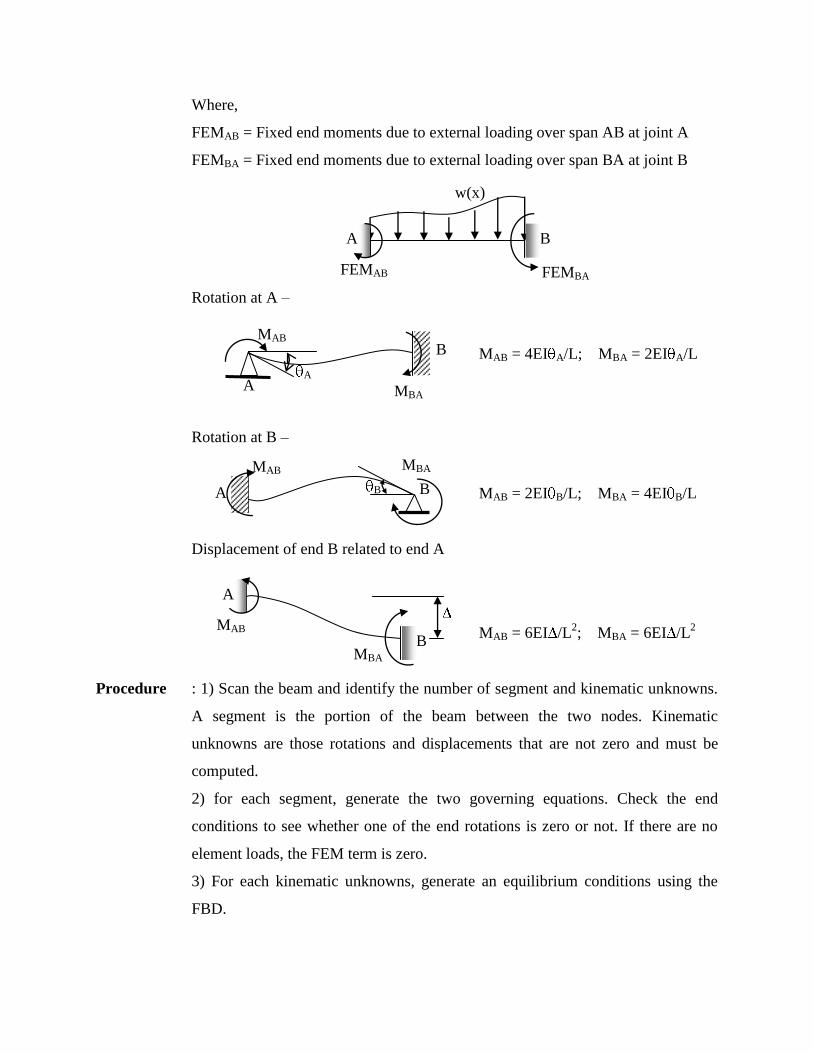
Where,
FEMAB = Fixed end moments due to external loading over span AB at joint A
FEMBA = Fixed end moments due to external loading over span BA at joint B
Rotation at A –
MAB = 4EI A/L; MBA = 2EI A/L
Rotation at B –
MAB = 2EI B/L; MBA = 4EI B/L
Displacement of end B related to end A
MAB = 6EI /L2; MBA = 6EI /L
2
Procedure : 1) Scan the beam and identify the number of segment and kinematic unknowns.
A segment is the portion of the beam between the two nodes. Kinematic
unknowns are those rotations and displacements that are not zero and must be
computed.
2) for each segment, generate the two governing equations. Check the end
conditions to see whether one of the end rotations is zero or not. If there are no
element loads, the FEM term is zero.
3) For each kinematic unknowns, generate an equilibrium conditions using the
FBD.
w(x)
B A
FEMBA FEMAB
MAB
MBA
B
A A
B
MBA MAB
A B
B
A
MBA
MAB
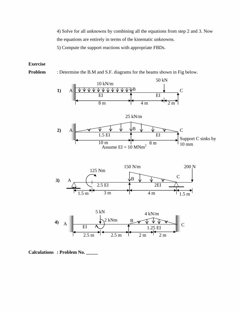
4) Solve for all unknowns by combining all the equations from step 2 and 3. Now
the equations are entirely in terms of the kinematic unknowns.
5) Compute the support reactions with appropriate FBDs.
Exercise
Problem : Determine the B.M and S.F. diagrams for the beams shown in Fig below.
Calculations : Problem No. _____
10 kN/m 50 kN
B C A EI EI
8 m 4 m 2 m
1)
25 kN/m
B C A 1.5 EI EI
10 m 8 m
2)
Support C sinks by
10 mm Assume EI = 10 MNm
2
150 N/m
B C A
2.5 EI 2EI
3 m 4 m
3)
200 N 125 Nm
1.5 m 1.5 m
4 kN/m
B C A
EI 1.25 EI
2 m
4)
2 m 2.5 m 2.5 m
5 kN
2 kNm

Conclusion :
References : 1. Maney, George A.(1915). Studies in Engineering. Minneapolis: University of
Minnesota.
Date:
Experiment -
Verification of Strain Energy Method by using Standard Structural Analysis
Software
Aim : Verification of strain energy method by using some standard structural analysis
software.
Theory : Energy principles are used to determine displacement in structures and
redundant action of an indeterminate structures. Its application is not only in
elementary analysis but also in advanced analysis and finite element methods.
Energy principles and principles of structural analysis are based on Newton‟s
laws of motion. Some significant concepts about force and energy are explained
here.
Work is done when a force acting on a body displaces it from its original position.
It is equal to product of the force applied and distance moved by its point of
application in the direction of force applied.
When a force displaces a body. The body receives either Kinetic Energy (if its
velocity is changed) or potential energy (if its position in the gravitational field is
changed).
If the force applied results in the distortion (or deformation) of the body, the work
done by the force is stored in the body as strain energy.
Strain energy is released in elastic bodies on removal of the loads. Strain energy
can be visualized as another form of potential energy and is sometimes referred to
as internal work done.
It is generally assumed that energy is converted from one form to another within a
given structural system, and no energy is dissipated in vibrations or as heat. This
is ideal situation, which may not always be realized in practice. This assumption,
however, does not often leads to serious errors in practical structures, especially
when steady loads are applied. Since the total energy of a system remains
constant, the algebraic sum of external and internal work done must be zero.
Computation of real energy can be tedious because of high order terms involved.
However, the concepts of strain energy can be applied to determine displacements
in a structure by making use of principle of minimum energy of a system. This
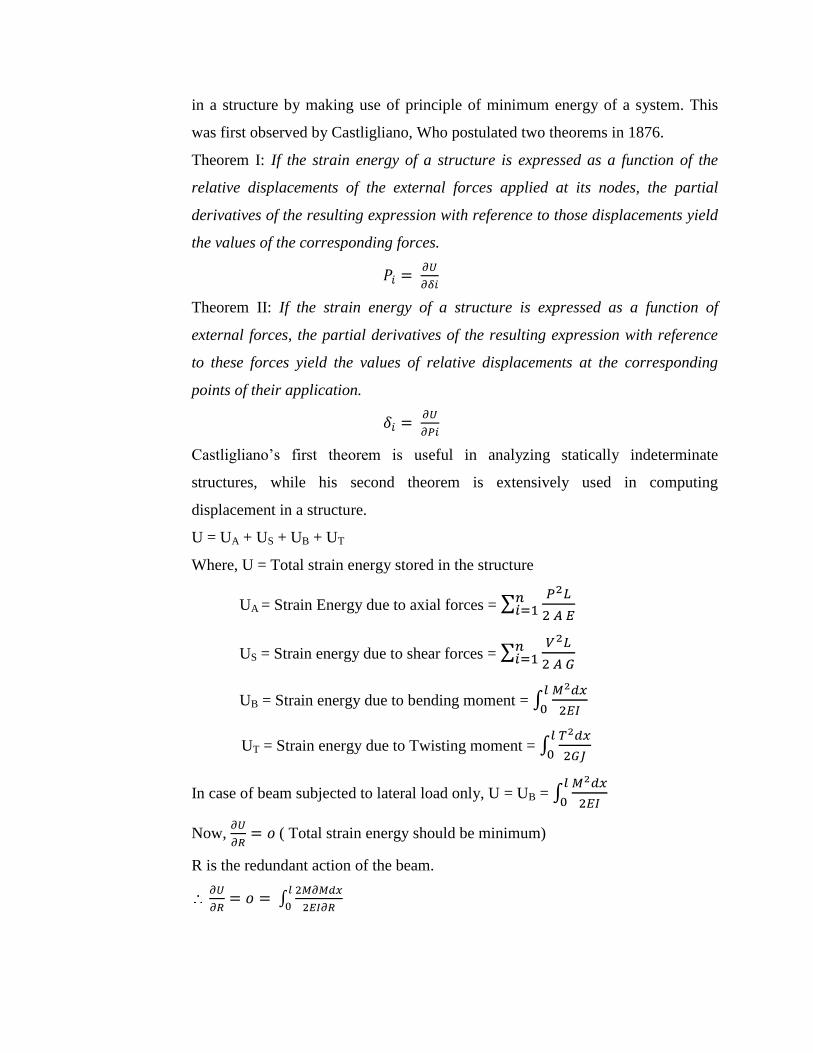
was first observed by Castligliano, Who postulated two theorems in 1876.
Theorem I: If the strain energy of a structure is expressed as a function of the
relative displacements of the external forces applied at its nodes, the partial
derivatives of the resulting expression with reference to those displacements yield
the values of the corresponding forces.
Theorem II: If the strain energy of a structure is expressed as a function of
external forces, the partial derivatives of the resulting expression with reference
to these forces yield the values of relative displacements at the corresponding
points of their application.
Castligliano‟s first theorem is useful in analyzing statically indeterminate
structures, while his second theorem is extensively used in computing
displacement in a structure.
U = UA + US + UB + UT
Where, U = Total strain energy stored in the structure
UA = Strain Energy due to axial forces =
US = Strain energy due to shear forces =
UB = Strain energy due to bending moment =
UT = Strain energy due to Twisting moment =
In case of beam subjected to lateral load only, U = UB =
Now, ( Total strain energy should be minimum)
R is the redundant action of the beam.
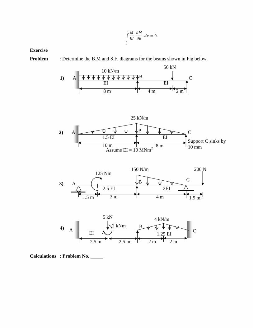
Exercise
Problem : Determine the B.M and S.F. diagrams for the beams shown in Fig below.
Calculations : Problem No. _____
10 kN/m 50 kN
B C A EI EI
8 m 4 m 2 m
1)
25 kN/m
B C A 1.5 EI EI
10 m 8 m
2)
Support C sinks by
10 mm Assume EI = 10 MNm
2
150 N/m
B C A
2.5 EI 2EI
3 m 4 m
3)
200 N 125 Nm
1.5 m 1.5 m
4 kN/m
B C A
EI 1.25 EI
2 m
4)
2 m 2.5 m 2.5 m
5 kN
2 kNm
Conclusion :
References : 1) Castligliano, C. A. P., The Theory of Equlibirium of Elastic Systems and Its
Applications, translated by E. S. Andrews with a new introduction and
biographical portrait section by G. A. Oravas, Dover Publications, Inc., New
York, 1966.
Date:
Experiment -
Study of Three Hinged Arch
Aim : Study of Three Hinged Arch.
Theory : An Arch may be visualized as a beam curved in elevation with convexity
upward which is restrained at its ends from spreading outwards under the action
of downward vertical loading. Arches have a long and interesting history through
several countries and their development spans over several countries. Etruscans,
people of Asiatic origin who invaded northern Italy around 1300 B.C., apparently
used in recorded history. Ancient Egyptians, Assyrians and Babylonians also
knew the advantages of arches, and used them extensively as architectural units.
The support of arch must be strong enough to develop horizontal thrust. In some
cases, horizontal thrust can be developed by means of a tie rod connecting the two
end of an arch.
Arches are very efficient forms of structural elements that develop only small
B.M. and resist external loads predominantly through axial compression. The
central line of an arch should be approximately, as close as possible to the
funicular polygon for dead load and at least a part of live load so that the B.M. are
small. This concept is called as Theoretical arch concept. Circular segments,
parabolas and multicentre circular curves provide ideal shapes to the approximate
funicular polygons for usual loading conditions.
Arches can be classified in several ways; on the basis of materials, shape and
structural systems. Structural shape/configuration permits classification of arches
as three-hinged, two-hinged, two-hinge with tie rod, suspended tie arch and fixed
arch.
Arches are used in buildings either for their functionality and aesthetics. Their use
in other structures is also extensive on account of their efficient structural
performance. Bridges, dams and large subterranean structures make use of arch
profiles for safety and economy.
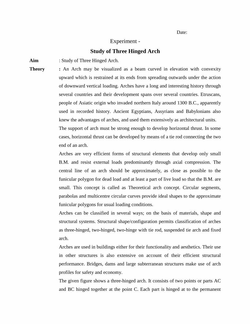
The given figure shows a three-hinged arch. It consists of two points or parts AC
and BC hinged together at the point C. Each part is hinged at to the permanent
support like an abutment at the lower ends (A and B). Hinge C, is provided at the
highest point of the centre line of the arch. The horizontal distance between the
lower ends A and B is called the span of the arch. When ends A and B are at the
same level, the height of the crown (point C), above the level of the ends is called
the rise of the arch.
Any external loads tends to cause an increase in the span length, as horizontal and
vertical movement are not possible. Reactions at both ends A and B will have
both horizontal and vertical components. The horizontal component of reactions
are equal if there is no horizontal applied load over the arch. By using MC = 0, we
can easily find out the horizontal reactive component whereas the vertical
reactions will get from MA = 0 and FY = 0. The difference between beam and
arch is that in case of arch a horizontal thrust is induced at each support which
provides a hogging moment Hy at any section. This is called the H moment at
section X-X.
Actual BM at X-X = Beam moment at X-X – H moment at X-X.
Taking moment about C,
Va . (L/2) = H.h + W1((L/2)-a)
Hence, H is calculated.
The bending moment at section XX, „x‟ distance from support A is
MX = VA. x – W1(x-a) – H.y
In case of parabolic arch the numerical relation between x and y is
Crown, MC = 0,
Rise, yc
Span
C
A B HB HA
VA VB
y
x
W1
a

Advantages : 1) The sagging moments are compensated by the hogging produced by
horizontal reaction.
2) For the same material of construction, span, thickness of arches is less than that
of beams, hence more economical.
3) More resistance to temperature stresses.
4) Three hinged arches adjust themselves in case of yielding of support and so
does not fail.
Disadvantages: 1) They are difficult to construct.
3) Three hinged arch fail easily if any of the horizontal support fails.
References : 1) S.P.Gupta, G.S. Pandit and R. Gupta.(1999), “Theory of Structures.” Volume
II, Tata Mc-Graw Hill Publishing company limited, New Delhi.
Date:
Experiment No -
Study of Non-Destructive Testing
(Schmidt Rebound Hammer Test)
Aim : To determine the strength of concrete member by rebound hammer test.
Theory : Importance and need of non-destructive testing
It is often necessary to test concrete structures after the concrete has hardened
to determine whether the structure is suitable for its designed use. Ideally such
testing should be done without damaging the concrete. The tests available for
testing concrete range from the completely non destructive, where there is no
damage to the concrete, through those where the concrete surface is slightly
damaged, to partially destructive tests, such as core tests and pullout and pull
off tests, where the surface can be repaired after the test. The range of
properties that can be assessed using non-destructive test is quite large and
includes such fundamental parameters as density, elastic modulus and strength
as well as surface hardness and surface absorption etc. In some cases it is also
possible to check the quality of workmanship and structural integrity by the
ability to detect voids, cracking and delamination. Non destructive testing can
be applied to both old and new structures.
Basic Methods for NDT of Concrete structures
The following methods, with some typical applications, have been used for the
NDT of concrete.
a) Visual inspection, which is an essential part of NDT.
b) Half cell electrical potential method, used to detect corrosion potential of
reinforcing bars in concrete.
c) Schmidt/rebound hammer test, used to evaluate the surface hardness of
concrete.
d) Carbonation depth measurement test, used to determine whether moisture
has reached the depth of the reinforcing bars and hence corrosion may
occurring.
e) Permeability test, used to measure the flow of water through the concrete.
f) Radiographic testing, used to detect void of concrete and the position of
stressing ducts.
g) Ultrasonic pulse velocity testing, mainly used to measure the sound velocity
of the concrete and hence compressive strength of concrete.
h) Infrared theromography, used to detect voids, delamination and other
anomalies in concrete and also detect water entry points in buildings.
Fundamental principle
The Schmidt rebound hammer is principally a surface hardness tester. It works
on the principle that the rebound of an elastic mass depends on the hardness of
the surface against which the mass impinges. There is little apparent
theoretical relationship between the strength of concrete and the rebound
number of the hammer. However, within limits, empirical correlations have
been established between strength properties and the rebound number. Further,
Kolek has attempted to establish a correlation between the hammer rebound
number and the hardness as measured by the Brinell method.
EQUIPMENT FOR SCHMIDT/REBOUND HAMMER TEST
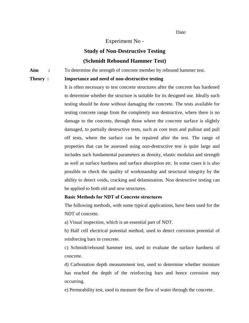
The Schmidt rebound hammer is shown in Fig. 1. The hammer weighs about
1.8 kg and is suitable for use both in a laboratory and in the field. A schematic
cutaway view of the rebound hammer is shown in Fig. 2. The main
components include the outer body, the plunger, the hammer mass, and the
main spring. Other features include a latching mechanism that locks the
hammer mass to the plunger rod and a sliding rider to measure the rebound of
the hammer mass. The rebound distance is measured on an arbitrary scale
marked from 10 to 100. The rebound distance is recorded as a “rebound
number” corresponding to the position of the rider on the scale.
FIG. 1. Schmidt rebound hammer.
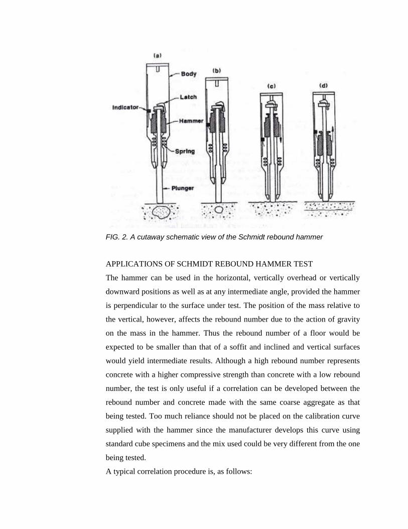
FIG. 2. A cutaway schematic view of the Schmidt rebound hammer
APPLICATIONS OF SCHMIDT REBOUND HAMMER TEST
The hammer can be used in the horizontal, vertically overhead or vertically
downward positions as well as at any intermediate angle, provided the hammer
is perpendicular to the surface under test. The position of the mass relative to
the vertical, however, affects the rebound number due to the action of gravity
on the mass in the hammer. Thus the rebound number of a floor would be
expected to be smaller than that of a soffit and inclined and vertical surfaces
would yield intermediate results. Although a high rebound number represents
concrete with a higher compressive strength than concrete with a low rebound
number, the test is only useful if a correlation can be developed between the
rebound number and concrete made with the same coarse aggregate as that
being tested. Too much reliance should not be placed on the calibration curve
supplied with the hammer since the manufacturer develops this curve using
standard cube specimens and the mix used could be very different from the one
being tested.
A typical correlation procedure is, as follows:
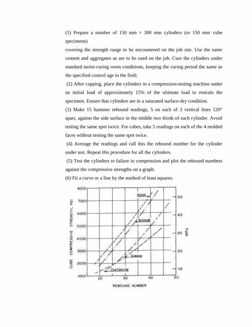
(1) Prepare a number of 150 mm × 300 mm cylinders (or 150 mm3 cube
specimens)
covering the strength range to be encountered on the job site. Use the same
cement and aggregates as are to be used on the job. Cure the cylinders under
standard moist-curing room conditions, keeping the curing period the same as
the specified control age in the field.
(2) After capping, place the cylinders in a compression-testing machine under
an initial load of approximately 15% of the ultimate load to restrain the
specimen. Ensure that cylinders are in a saturated surface-dry condition.
(3) Make 15 hammer rebound readings, 5 on each of 3 vertical lines 120°
apart, against the side surface in the middle two thirds of each cylinder. Avoid
testing the same spot twice. For cubes, take 5 readings on each of the 4 molded
faces without testing the same spot twice.
(4) Average the readings and call this the rebound number for the cylinder
under test. Repeat this procedure for all the cylinders.
(5) Test the cylinders to failure in compression and plot the rebound numbers
against the compressive strengths on a graph.
(6) Fit a curve or a line by the method of least squares.
Correlation curves produced by different researchers. (Greene curve used
Type N hammer; others used Type N-2).
RANGE AND LIMITATIONS OF SCHMIDT REBOUND HAMMER TEST
Although the rebound hammer does provide a quick, inexpensive method of
checking the uniformity of concrete, it has some serious limitations. The
results are affected by :
1. Smoothness of the test surface
2. Size, shape and rigidity of the specimen
3. Age of the specimen
4. Surface and internal moisture conditions of concrete
5. Type of coarse aggregate
6. Type of cement
7. Carbonation of the concrete surface
Procedure: The method of using the hammer is explained using Fig.2. With the hammer
pushed hard against the concrete, the body is allowed to move away from the
concrete until the latch connects the hammer mass to the plunger, Fig.2a. The
plunger is then held perpendicular to the concrete surface and the body pushed
towards the concrete, Fig.2b. This movement extends the spring holding the
mass to the body. When the maximum extension of the spring is reached, the
latch releases and the mass is pulled towards the surface by the spring, Fig.2c.
The mass hits the shoulder of the plunger rod and rebounds because the rod is
pushed hard against the concrete, Fig.2d. During rebound the slide indicator
travels with the hammer mass and stops at the maximum distance the mass
reaches after rebounding. A button on the side of the body is pushed to lock
the plunger into the retracted position and the rebound number is read from a
scale on the body.
Observations:

Results :
Conclusion :
Date:
Experiment No -
Influence Line Diagram and moving loads application in bridges
Aim : Study the influence line diagram and special application of moving
loads in bridges.
Theory : Superimposed loads on structures are not always static. Bridges, for
instance, are subjected to moving loads whose effects on structures vary
depending upon the position occupied by the load systems. For any
system, there will be at least one position of the given loads, for which
their effects (B.M., S.F., A.F. or deflections) will be maximum. In some
cases, it will be possible to locate the position of loads for maximum. In
some cases, it will be possible to locate the position of loads for
maximum effects by inspection or intuition. Trial and error process may
be adequate in few other cases. However, a systematic procedure to
determine the critical effects of moving loads is offered by the concept
of influence lines (I.L.).
The variation of significant effects in a structures caused by a moving
unit load can be expressed as a function of the position of the load. This
variation, when expressed in a graphical form, is known as the
influence diagram. In the case of linear structures such as beams,
trusses and frames, these diagrams are called influence lines.
The concept of I.L. was first formulated in 1867 by E. Winkler, a
German scientist. The importance of the concept was not realized until
after 1887, when Heinrich Mueller-Breslau, another German, developed
in further by extending the principle of reciprocity enunciated by J. C.
Maxwell. Mueller-Breslau also discovered a simple method of
developing influence diagrams qualitatively (Which bears his name).
An influence line, in general, can be defined as the graphical
representation of the variation of a specified parameter at a section in a
structure, when a unit load moves along its length.
Influence diagrams can be drawn for statically determinate as well as
indeterminate structures. They can be drawn for structures comprising
linear elements (beams, arches and frames), and for planar structures
(plates); in the latter case they are called influence surfaces.
The ordinates of the influence line for any chosen reaction component
may be determined by adopting any one of the following methods:
i) Direct Method
In this approach, the unit load is placed at any point P and the value of
the chosen reaction component is determined by using any one of the
methods.
ii) Indirect Method
The indirect method is based on Muller Breslau‟s principle, accordingly
the constraints corresponding to the chosen reaction component is
released and the chosen reaction component is given a unit
displacement while all other reaction components are kept undisplaced.
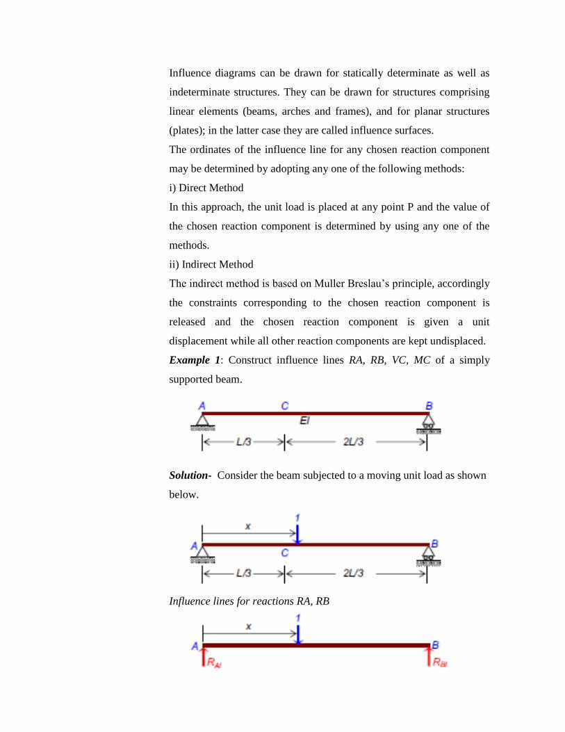
Example 1: Construct influence lines RA, RB, VC, MC of a simply
supported beam.
Solution- Consider the beam subjected to a moving unit load as shown
below.
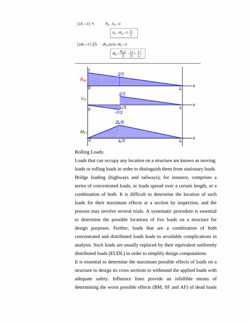
Influence lines for reactions RA, RB
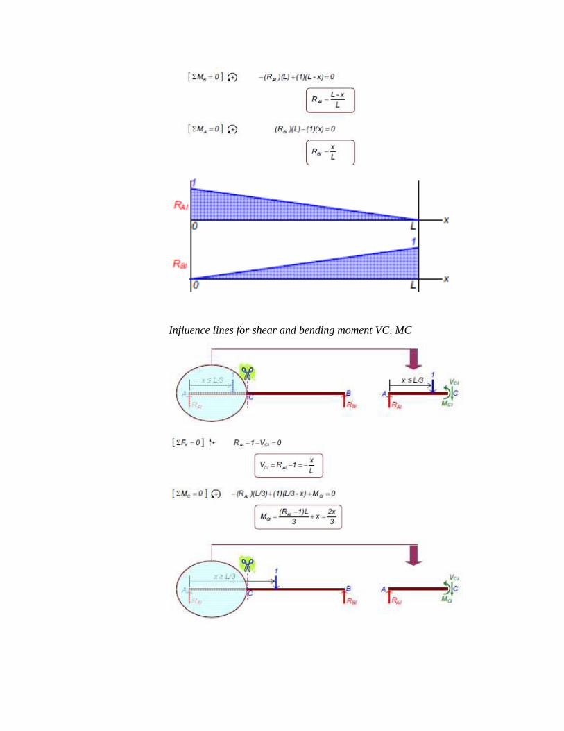
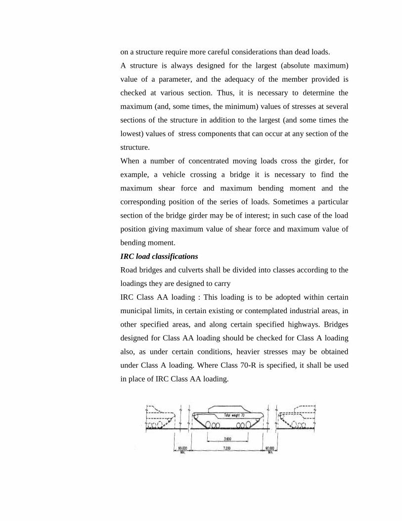
Influence lines for shear and bending moment VC, MC
Rolling Loads:
Loads that can occupy any location on a structure are known as moving
loads or rolling loads in order to distinguish them from stationary loads.
Bridge loading (highways and railways), for instance, comprises a
series of concentrated loads, or loads spread over a certain length, or a
combination of both. It is difficult to determine the location of such
loads for their maximum effects at a section by inspection, and the
process may involve several trials. A systematic procedure is essential
to determine the possible locations of live loads on a structure for
design purposes. Further, loads that are a combination of both
concentrated and distributed loads leads to avoidable complications in
analysis. Such loads are usually replaced by their equivalent uniformly
distributed loads (EUDL) in order to simplify design computations.
It is essential to determine the maximum possible effects of loads on a
structure to design its cross sections to withstand the applied loads with
adequate safety. Influence lines provide an infallible means of
determining the worst possible effects (BM, SF and AF) of dead loads
on a structure require more careful considerations than dead loads.
A structure is always designed for the largest (absolute maximum)
value of a parameter, and the adequacy of the member provided is
checked at various section. Thus, it is necessary to determine the
maximum (and, some times, the minimum) values of stresses at several
sections of the structure in addition to the largest (and some times the
lowest) values of stress components that can occur at any section of the
structure.
When a number of concentrated moving loads cross the girder, for
example, a vehicle crossing a bridge it is necessary to find the
maximum shear force and maximum bending moment and the
corresponding position of the series of loads. Sometimes a particular
section of the bridge girder may be of interest; in such case of the load
position giving maximum value of shear force and maximum value of
bending moment.
IRC load classifications
Road bridges and culverts shall be divided into classes according to the
loadings they are designed to carry
IRC Class AA loading : This loading is to be adopted within certain
municipal limits, in certain existing or contemplated industrial areas, in
other specified areas, and along certain specified highways. Bridges
designed for Class AA loading should be checked for Class A loading
also, as under certain conditions, heavier stresses may be obtained
under Class A loading. Where Class 70-R is specified, it shall be used
in place of IRC Class AA loading.
IRC Class A Loading: This loading is to be normally adopted on all
roads on which permanent bridges and culverts are constructed.
IRC Class B Loading: This loading is to be normally adopted for
temporary structures and for bridges in specified areas. Structure with
timber span are to be consider as temporary structures.
Conclusion(s) :