S tationkeeping - University of Toronto T-Spacetspace.library.utoronto.ca/bitstream/1807/11782/1/mq29367.pdf · Abstract The Space Shuttle middeck is an unlikeIy place to hd a fiee-

S tationkeeping in the Space Shuttle Middeck: Preliminary Design for the DICE Bus Module

Johanne Heald

A thesis submitted in conformity with the requirements for the degree of Master of Applied Science

Institute for Aerospace Studies University of Toronto

@Copyright by Johanne Heald (1997)

395 Wellington Street 395, rue Wellington Ottawa ON K I A ON4 Ottawa ON K I A ON4 Canada Canada

Your file Votre refërence

Our file Notre reklr8nce

The author has granted a non- L'auteur a accordé une licence non exclusive licence allowing the exclusive permettant à la National Library of Canada to Bibliothèque nationale du Canada de reproduce, loan, distribute or sel1 reproduire, prêter, distribuer ou copies of this thesis in microform, vendre des copies de cette thèse sous paper or electronic formats. la fome de microfichelfilm, de

reproduction sur papier ou sur format électronique.

The author retains ownership of the L'auteur conserve la propriété du copyright in this thesis. Neither the droit d'auteur qui protège cette thèse. thesis nor substantial extracts fkom it Ni la thèse ni des extraits substantiels may be printed or otherwise de celle-ci ne doivent être imprimés reproduced without the author's ou autrement reproduits sans son permission. autorisation.

Abstract

The Space Shuttle middeck is an unlikeIy place to h d a fiee- fioating satellite. That, however, is just what DICE proposes to be: an untethered free-flyer under astronaut supervision. In support of the DICE project , this thesis examines the disturbance forces to which that free-flyer would fa11 prey, proposes a design for an actuation system which would counter those disturbances, and simulates the control of this actuation system.

From a survey of middeck disturbance forces, five significant ones are examined: middeck air circulation, solar radiation pressure, atmospheric drag, graviiy gradient torque, and orbital offset between Shuttle Orbiter and DICE mass centers. A simulation of these forces is created in XMath. Middeck air circulation proves to be the greatest disturbance, exerting forces up to 10-~ N and torques up to IOy4 Nm. In reply to these disturbances, an actuation system is proposed. It re-circulates middeck cabin air through the DICE bus and ejects it through 3 nozzle clusters in order to produce a net thrust. The airflow created by such an actuation system is characterised, while mock-up condit ions, t hruster location, and valve position are varied. The force output of one nozzle on the mock-up most faithful to curent design is measured to be 10-2 N.

Acknowledgment s

The author wishes to acknowledge the contributions of the following persons or agencies in support of this thesis:

Dr. P. C. Hughes, for supervising this thesis and assisting in its final production

NSERC and Canadian Space Agency, for financial support

rn Dr. J . D. DeLaurier, for the cheerful loan of equipment

Eric Choi, Robert Zee, Robert Bauer, and James Crawford, al1 fel- low students at UTIAS, for their multitudes of advice, assistance, and patience

Kieran Carroll, Don McTavish, and Stephen Piggott, colleagues on the DICE Project at Dynacon Enterprises, for ensuring progress and relevance to the project

rn Finally, my parents, sister, and friends - al1 those who were with me along the way

iii

Contents

1 Stationkeeping for a Purpose 1 . . . . . . . . . . . . . . . . . . . . . . . 1.1 Background on DICE 1

. . . . . . . . . . . . 1.2 Development of a Stationkeeping System 7 . . . . . . . . . . . . . . . . . . . . . . . . . 1.2.1 Motivation 7

. . . . . . . . . . . . . . . . . . . . . . 1.2.2 Previous Work 10 . . . . . . . . . . . . . . . . . . . . . . . . 1.3 Scope of This Work 11

. . . . . . . . . . . . . . . . . . . . 1.3.1 Aim and Structure 11 . . . . . . . . . . . . . . . . . . . . . 1.3.2 Task Breakdown 12

2 A Disturbing Environment 13 . . . . . . . . . . . . . . . . . . . . . . . . 2.1 Rames of Reference 13

. . . . . . . . . . . . . . . . . 2.2 A Survey of Disturbance Forces 14 . . . . . . . . . . . 2.3 Mathematical Formulation of Disturbances 16

. . . . . . . . . . . . . . . . . 2.3.1 Middeck Air Circulation 16 . . . . . . . . . . . . . . . . . . . . . . . 2.3.2 Orbital Offset 19

. . . . . . . . . . . . . . . . . 2.3.3 Solar Radiation Pressure 21 . . . . . . . . . . . . . . . . . . . . 2.3.4 Atmospheric Drag 24

. . . . . . . . . . . . . . . . . 2.3.5 Gravity Gradient Torque 27

3 Disturbance Forces in Simulation 31 . . . . . . . . . . . . . . . . . . . . . . . . . . 3.1 Apparent Forces 31

. . . . . . . . . . . . . . . . . . . . . . . . 3.1.1 Formulation 31 . . . . . . . . . . . . . . . . . . . . . . . . . . . 3.1.2 Results 33

. . . . . . . . . . . . . . . . 3.1.3 Total Orbiter Disturbances 44 . . . . . . . . . . . . . . . . . . . . . . . . . . . . 3.2 Real Forces 46

. . . . . . . . . . . . . . . . . . . . . . . . 3.2.1 Formulation 46 . . . . . . . . . . . . . . . . . . . . . . . . . . . 3.2.2 Results 47

. . . . . . . . . . . . . . 3.2.3 Total DICE Hub Disturbances 56

3.3 Summary of the Simulation Results . . . . . . . . . . . . . . . 58

4 Air on the Move: Actuation 59 4.1 Design Requirements . . . . . . . . . . . . . . . . . . . . . . . 59

. . . . . . . . . . . . . . . . . . . . . . 4.2 Design Characteristics 61 . . . . . . . . . . . . . . . . . . . 4.2.1 Actuator Subsystems 61

. . . . . . . . . . . . . . . 4.2.2 Implementation on the IPM 62 . . . . . . . . . . . . . 4.2.3 Lessons Learned from the IPM 62

. . . . . . . . . . . . . . . . . . . . . . . . . 4.3 Design Evaluation 68

5 Stationkeeping Put to the Test 69 . . . . . . . . . . . . . . . . . . . . . 5.1 A Forum for Verification 69

. . . . . . . . . . . . . 5.2 Bus Mock-up Design and Construction 70 . . . . . . . . . . . . . . . . . . . . . . . . . . . . 5.3 Test Results 73

. . . . . . . . . . . . . . . . . . 5.3.1 Preliminary IPM Tests 73 . . . . . . . . . . . . . . . . . . . . 5.3.2 Bus Mock-up Tests 81

. . . . . . . . . . . . . . . . . . . . . . . . 5.4 Actuator Modelling 90 . . . . . . . . . . . . . . . 5.4.1 Trends in Empirical ResuIts 90

5.4.2 Simulation ModelIing of Actuators . . . . . . . . . . . 90 . . . . . . . . . . . . . . . . 5.4.3 Controlling the Actuators 92

6 Some Concluding Remarks 101 . . . . . . . . . . . . . . . . . . . . 6.1 What Has Been Learned? 101

. . . . . . . . . . . . . . . 6.2 Recommendations for Fùrther Work 102

A Thesis Task List 109

B Orbiter Characteristics

C XMath/Systembuild Code for Disturbances 113 . . . . . . . . . . . . . . . . . . . . . . . . C . 1 set .parameters.msf 114

. . . . . . . . . . . . . . . . . . . . . . . . . . . . . . C.2 drag.msf 117 . . . . . . . . . . . . . . . . . . . . . . . . . . . . . C.3 density.msf 119

. . . . . . . . . . . . . . . . . . . . . . . . . . . . . . C.4 so1ar.msf 120 . . . . . . . . . . . . . . . . . . . . . . . . . . . . . C.5 orient.msf 123

. . . . . . . . . . . . . . . . . . . . . . . . . . . (2.6 torquecp.msf. 126 . . . . . . . . . . . . . . . . . . . . . . . . . . . . . C.7 fframe.msf 127 . . . . . . . . . . . . . . . . . . . . . . . . . . . . . C.8 frame.msf 128

. . . . . . . . . . . . . . . . . . . . . . . . C.9 Systembuild Blocks 130

. . . . . . . . . . . . . . . . . . . . . C.9.1 Hub Disturbances 131 . . . . . . . . . . . . . . . . . . . . C.9.2 Atmospheric Drag 133

. . . . . . . . . . . . . . . . . . . . . . C.9.3 Solar Radiation 135 . . . . . . . . . . . . . . . . . C.9.4 Gravity Gradient Torque 137

. . . . . . . . . . . . . . C . 9.5 Total Run-time Disturbances 139 . . . . . . . . . . . . . . . . . . . . . . . . C.9.6 Locker Fans 141

. . . . . . . . . . . . . . . . . . . C.9.7 Orbital Offset Forces 147

D Empirical Data from Air FIow Tests 149 . . . . . . . . . . . . . . . . . . . . . . . . . . . . . D.1 IPM Trials 150

. . . . . . . . . . . . . . . . . . . . . . . . . . . . D.2 BMU Trials 154 . . . . . . . . . . . . . . . . . . . . . . . . D.2.1 Empty Bus 154

. . . . . . . . . . . . D.2.2 Interior Elements Installed in Bus 157

E XMath/Systembuild Code for Actuators 161 . . . . . . . . . . . . . . . . . E.l Additions to set-parameters.msf 161

. . . . . . . . . . . . . . . . . . . . . . . . E.2 Systembuild Blocks 163

. . . . . . . . . . . . . . . . . . . . . . . . E.2.1 Air Thruster 163 . . . . . . . . . . . . . . . . . . E . 2.2 Stationkeeping System 165 . . . . . . . . . . . . . . . . . . E.2.3 Controller in One DOF 167 . . . . . . . . . . . . . . . . . . E.2.4 Six Channel Controller 169

vii

viii

List of Figures

. . . . . . . . . . . . . 1.1 Examples of Flexible Space Structures 3 1.2 Test articles for Daisy and DICE . . . . . . . . . . . . . . . . 5

. . . . . . . . . . . . . . . . . . . . . . . . . 1.3 RadarSat satellite 8

. . . . . . . . . . . . . . . . . . . . . . . . 2.1 Frames of Reference 14 2.2 ARS Vent Locations in the Orbiter Middeck (in inches) . . . . 17

. . . . . . . . . . . . . . . . . . . . . . . . 2.3 Air Jet in middeck 18 2.4 Target (Orbiter) and Chase (DICE) Vehicles in Orbit . . . . . 20

. . . . . . . . . . . . . . . . . . . 2.5 Radiation on an Earth Orbit 22 . . . . . . . . . . . 2.6 Orbiter Surface Area Perpendicular to Sun 23

. . . . . . . . . . . . . . . . . 2.7 Atrnospheric Density Variation 25 . . . . . . . . . . . . . 2.8 Gravity Gradient Force on the Shuttle 28

3.1 Shuttle in Orientation 1. Nose Forward. PBDs Away fiom Earth 3.2 Shuttle in Orientation 1. Nose Away from Earth. PBDs Aft . . 3.3 Atmospheric Drag at 200 km in Orientation 1 . . . . . . . . . 3.4 Atmospheric Drag at 300 km in Orientation 1 . . . . . . . . . 3.5 Atmospheric Drag at 400 km in Orientation 1 . . . . . . . . . 3.6 Atmospheric Drag at 450 km in Orientation 1 . . . . . . . . . 3.7 Solar Radiation Pressure. Start Time = O sec . . . . . . . . . 3.8 Solar Radiation Pressure. Start Time = -1000 sec . . . . . . . 3.9 Solar Radiation Pressure. Start Time = -2000 sec . . . . . . . 3.10 Gravity Gradient Torque: Orbiter Nose Forward . . . . . . . . 3.11 Apparent Forces in Concert . . . . . . . . . . . . . . . . . . . 3.12 Orbital Offset Acceleration: Orbiter Nose Forward . . . . . . . 3.13 Orbital Offset Acceleration: Orbiter Nose Up . . . . . . . . . . 3.14 Orbital Offset Acceleration: DICE off Cargo Bay Center Line 3.15 Force due to Single Fan - Middeck Forward . . . . . . . . . . .

. . . . . . . . . . . . . 3.16 Force due to Single Fan - Middeck Aft

. . . . . 3.17 Force due to Multiple Fans Middeck Forward and Aft 55 3.18 Real Disturbance Forces Acting in Concert (SVS fiame) . . . 57

Alternative Nozzle Positioning on DICE Bus . . . . . . . . . . 63 . . . . . . . . . . . . . . . . . . . . . Proposed Nozzle Cluster 63

Performance Curves for Axial Flow Fan . . . . . . . . . . . . . 65 Performance Curves for Centrifugal Backward-Bladed Fan . . 65 Performance Curves for Centrifuga1 Radial-Bladed Fan . . . . 66 Performance Curves for Centrifuga1 Forward-Bladed Fan . . . 66 Operation of Two Identical Fans in Parallel . . . . . . . . . . 67 Effect of Change of Ambient Air Density on Fan and System . 67

. . . . . . . . . . . . . . . . 5.1 The Bus Mock.up. Exterior View 71 5.2 The Bus Mock.up. Interior View with Selected Components . 71

. . . . . . . . . . . . . . . . . . . 5.3 Bus Mock-Up Specifications 72 5.4 Apparatus for Air Flow Tests . . . . . . . . . . . . . . . . . . 74 5.5 Thruster and Nozzle System in IPM Interior . . . . . . . . . . 75 5.6 Pressure Profiles of the Side IPM Thrusters . . . . . . . . . . 76 5.7 Velocity Profiles of Side IPM Thrusters . . . . . . . . . . . . . 77 5.8 Pressure and Velocity Profiles of IPM Main Thruster . . . . . 79 5.9 Pressure Profiles at Different IPM Wedge Angles . . . . . . . . 80 5.10 Air Pressure Profiles for Nozzles on the Bus Mock-up . . . . . 82 5.11 Air Velocity Profiles for Nozzles on the Bus Mock-up . . . . . 83 5.12 Thrust Distribution Amoung Bus Mock-up Nozzles . . . . . . 85 5.13 Thrust vs . Valve Position for Bus Mock-up . . . . . . . . . . . 86 5.14 Air Pressure a t Various Wedge Angles for Bus Mock-up . . . . 87 5.15 Location of Thrusters in DICE Rame of Reference . . . . . . 91 5.16 Results of Step Input without PID Control . . . . . . . . . . . 94 5.17 Results of Step Input with PID Control . . . . . . . . . . . . . 96 5.18 Results of Disturbance Input . . . . . . . . . . . . . . . . . . . 97 5.19 Control of Several Degrees of F'reedom . . . . . . . . . . . . . 99

C.l Precalculated Hub Disturbances . . . . . . . . . . . . . . . . . 132 . . . . . . . . . . . . . . . . . . . . . . . . . C.2 Atmospheric Drag 134

. . . . . . . . . . . . . . . . . . . . . C.3 Solar Radiation Pressure 136

. . . . . . . . . . . . . . . . . . . . . C.4 Gravity Gradient Torque 138 . . . . . . . . . . . . . . . . . . . . C.5 Runtime Hub Disturbances 140

. . . . . . . . . . . . . . . . . C.6 Space Shuttie Middeck Lockers 142

. . . . . . . . . . . . . . . . . . . . C.7 Middeck Fan Formulation 144 . . . . . . . . . . . . . . . . . C.8 Air Jet as a Standard Deviation 146

. . . . . . . . . . . . . . . . . . . . . . . C.9 Orbital Offset Forces 148

. . . . . . . . . . . . . . . . . . . . E.1 Individual Thruster Mode1 164 . . . . . . . . . . . . . . . . . . E.2 Stationkeeping System Mode1 166

. . . . . . . . . . . . . . E.3 Controller for One Degree of F'reedom 168 . . . . . . . . . . . . . . . . . . . . . . . . . . . E.4 Fùll Controller 170

List of Tables

2.1 Area and Absorptivity of Orbiter Surfaces . . . . . . . . . . . 24 2.2 Diurnal Effect at 30 degrees latitude . . . . . . . . . . . . . . 27

D.1 Manometer Readings (mm) for Right Side Thruster . . . . . . 150 D.2 Mânometer Readings (mm) for Left Side Thruster . . . . . . . 151 D.3 Manometer Readings (mm) for Main Thruster . . . . . . . . . 152 D.4 Manometer Readings (mm) for Different Valve Positions, Left

. . . . . . . . . . . . . . . . . . . . . . . . . . . . . . Thruster 153 D.5 Manometer Readings (mm) for Left Thruster . . . . . . . . . . 154 D.6 Manometer Readings (mm) for Right Thruster . . . . . . . . . 155 D.7 Force Readings for Al1 Nozzles . . . . . . . . . . . . . . . . . . 156 D.8 Manometer Readings (mm) for Different Valve Positions, Left

. . . . . . . . . . . . . . . . . . . . . . . . . . . . . . Thruster 157 D.9 Force Readings for Al1 Nozzles . . . . . . . . . . . . . . . . . . 158 D . 10 Force (g) vs . Valve Position . . . . . . . . . . . . . . . . . . . 158 D . l l Force Time Variations . . . . . . . . . . . . . . . . . . . . . . 159

xiii

List of Symbols

Altitude (km) Reference altitude (km) Flow area (m2) Acceleration ( 3 ) Factor indicating turbulence (3.3 - 10) Speed of light (2.99 x 108 y ) Direction cosines Coefficient of drag Phase of the year Nozzle diameter (m) Force delivered by airflow (N) Force due to atmospheric drag (N) Frame of principle axes Solar radiation force (N) Acceleration due to gravity (9) Torque due to gravity (Nm) Shuttle inertia matrix Specific Impulse (9 or g) Absorptivity constant Gravitational constant for Earth (3.986 x 10l4Y) Mean orbital rate (y) Solar pressure (5) Principal axis of orbiting vehicle Aow rate ($) Principal axis of orbiting vehicle Separation between two vehicles (m) Distance from Earth CM to chase vehicle (m) Distance fiom CM to CP (m) Earth radius (6300km) Gas constant Distance from Earth CM to target vehicle (m) Density (3) Density at reference altitude (9) Principal axis of orbiting vehicle Shuttle surface area (m2) Time (sec) Temperatme (K)

xiv

T. Torque exerted by solar pressure (Nm) 9 Angle of umbra about Earth (rad) V Air velocity ( y ) vWis Air velocity along nozzle axis (5) vd Air velocity at nozzle exit ( y ) y Distance from nozzle exit along axis (m)

List of Acronyms

ARS ASVS BMW CM CP DICE FSS FTA IPM ISS MACE MAUE MIT MODE NASA NSERC PID PBD SI S 1 STA STS svs UTIAS

Air Recirculation System Advanced Space Vision System Bus Mock-up Center of Mass Center of Pressure Dynamics, Identification, and Control Experiment Flexible Space Structures Fluid Test Article Integrated Prototype Mode1 International Space Station Middeck Active Control Experiment Middeck Active Umbilical Experiment Massechusett s Institute of Technology Middeck O-Gravity Dynamics Experiment National Aeronautics and Space Administration Natural Science and Engineering Reseasch Council Proport ional, Integrator , Derivat ive Payload Bay Door Systeme Internationale System Identification Solid Test Article Space Sransportation System Space Vision System (see also ASVS) Univerisity of Toronto Institute for Aerospace Studies

xvi

Chapter 1

Stationkeeping for a Purpose

The subject of this thesis is the preliminary design of a stationkeeping system for the DICE project. In course of this design, a range of different aerospace fields will be dealt with: fluid flow, orbital mechanics, and rigid body attitude motion, to name a few. However, before any discourse on these subjects can take place, some background is necessary. Specifically, it is necessary to understand the context in which this thesis takes place, and the DICE Project as a whole. This chapter will cover that material, as well as describing the scope of this thesis itself.

1.1 Background on DICE

The DICE (Dynamics, Identification, and Control Experiment) Project was conceived in 1994 as a joint project between Dynacon Enterprises Ltd. and the Spacecraft Dynamics Group at the University of Toronto Institute for Aerospace Studies (UTIAS). Its aim is to study the dynamics and control of flexible space structures (FSS) using a fiee-flying module [30]. This goal raises several important questions about the project: What space structures are considered flexible? Why is it important to control them? How is it proposed to study them? And, of course, to what end?

First, consider the question of flexibility. The class of spacecraft which can be described as FSS must possess inherent physical flexibility. This is true of al1 spacecraft, of course - no structure is perfectly rigid. However, in orbit, many structures behave as though they were rigid, and can be treated as such, so long as extremely accurate positioning and pointing are not required.

Other spacecraft possess long, slender, spindly features, such as booms and sol= panels, which cannot be considered rigid by aay stretch of the imagi- nation. These features react to disturbance forces with large deflections and low frequency vibrations. In other words, there are two criteria for spacecraft flexibility : high point ing accuracy requirements, and high structural deflections or deformations. The Hubble Space Telescope, for instance, must keep a deep sky object steady in its field of view for a specified exposure time; it is an excellent example of a space structure which is considered flexible due to its high-accuracy pointing requirernents. The plans for the upcoming International Space Station cal1 for it to be a structure consisting of trusses and solar panels and modules al1 connected together; it is an example of a structure with high structural deformations.

In order to control the orbit of an FSS, it must be considered separately from rigid structures. Many of the control methods used with such rigid- behaving spacecraft cannot cope with the vibration hequencies involved with flexible structures. In dealing with FSS, necessity has been the mother of invention, and many controllers have evolved specifically to improve the ability to control the high deflections caused by excitation of flexible modes of vibration. In theory, that is. Al1 controllers that are successful on paper must also prove that they are successful on spacecraft. Therefore, control theory must be translated into algorithm and applied to a structure in order to demonstrate its utility.

Due to spacecraft complexity and high launch costs, ground testing has always been the method of choice for FSS control research and evaluation. However, a ground test cannot, by definition, simulate the single most important factor aflecting a spacecraft in orbit: the fiee-fa11 (often called O-g) environment. Ideally, one should conduct FSS control experiments in space, with little risk or required financial expenditure.

Enter the DICE Project, as well as its preceders, the MODE and MACE projects of MIT. These are Çee-fall experimental facilities, designed specifically to carry out procedures under the supervision of an astronaut in the American Space Shuttle middeck. Middeck experiments are an ideal solution to the quandary of FSS control researchers, since each of these projects provides a small testbed which features FSS characteristics. In the course of one shuttle mission, many control a l g o r i t h cm be tested. If further data is required later, the testbed is reusable, and can be flown again. This is a relatively low-risk, low-cost way for researchers to try out new control algori thms in space.

(a) Hubble Space Telescope

(b) International Space Station

Figure 1.1: Examples of $lexible Space Structures

The MODE project at MIT was the first to take advantage of this phi- losophy. The first version of this project, MODEl, flew on STS-48 and consisted of two test articles, both described in [8] : a fluid test article (FTA) which investigated nonlinear slosh efTects of contained fiuids in microgravity, and a structura1 test article (STA) which was used to investigate the microgravity dynamics of truss structures with nonlinear components. This second test article was of particular interest, since it impacted on an upcorning space project. It is proposed to construct the upcoming Interna- tional Space Station with a number of truss structures, similar to the STA. The results of data taken during the MODEl flight both in space and on the ground showed that gravity significantly alters the mode1 characteristics of flexible structures [8], and that existing linear models predicted the fluid slosh natural frequencies to within 5 to 35% [7].

The follow-on project to MODEl was originally designated MODE2, and then became known as MACE. The MACE project was flown aboard STS-67, and its objective was to develop controller techniques which could be used to evaluate algorithms for control of FSS. In contrat to the open- b o p dynamic tests used for MODE-1, MACE was intended to demonstrate high aut hority active structural control in O-g using closed-bop dynamics. The test article itself consisted of multiple platforms, and the goal was to use different control algorithms to maintain the pointing accuracy of one payload, while the other payload moved independently [NI.

Due to the success of the MODE and MACE experiments, reflight of the STA has been proposed to follow-up on issues which were neglected during MODE- 1.

The DICE project intends to take advantage of the success of MODE and MACE as Space Shuttle Orbiter experiments in FSS dynamics and control. The DICE test article ressembles a different class of spacecraft from the MODE and MACE variety, and is based on previous work done at UTIAS, on a ground facility called Daisy. In mimicking Daisy's structure, which consists of a central hub with flexible ribs, much of the expertise gained from Daisy can be extended to DICE. See Figure 1.2 for a visual representation of both Daisy and DICE.

The DICE experiment consists of the three elements which give it its name:

Dynarnics The DICE project deals specifically with flexible structures. Thus, the test acticle will exhibit two phenomena common to flexible space-

(a) Daisy

(b) DICE

Figure 1.2: Test articles for Daisy and DICE

5

craft: mode clustering and mode localization. These two phenomena are explained in [20]. Mode clustering simply means that many of the vibration modes have similar frequencies; thus, it can be difficult to in- dentify the contributions of each mode when using a sensor to measure their effect. Mode localization occurs when the shapes of the modes are changed out of all proportion in the vicinity of a small imperfection of the structure.

Identification System Identification (SI) involves the development of a mathematical model of the dynamics of a structure in question. A series of known, random disturbance forces and torques act on the structure, and, from the resulting output (e.g. displacements, velocities, and accelerations), a mathematical model for 'what happened in between' can be developed. It is the method of developing this mathematical model that differentiates different SI methods. One of the goals of the DICE project is to conduct on-board system identification using different methods, and to compare the results.

Control Control Systems involve the use of a mathematical model of the structural dynamics of a structure (provided by the SI work, above, or using other methods such as the Finite Element Method) and a feedback algorithm in order to effect changes in the position, orientation, velocity, and acceleration of a structure. In the case of the DICE project, it is desirable to control both the central hub (the rigid part) and the rib tips (the flexible part). Controllers used on the test article cover different designs, ranging fiom convent ional Single Input Single Output methods to more recent Multiple Input Multiple Out- put methods. One of the goals of the DICE project is to evaluate the performance of these different controllers [30].

In order to achieve these goals, the DICE test article must have certain physical characteristics. The preliminary design for the test article includes a rigid component (a central hub) and a flexible component (a set of flexible ribs) . The central hub provides power , sensing, actuation, and on-board control; the five ribs provide the flexible dynamics, and additional actuat ion from the rib tips.

1.2 Development of a Stationkeeping System

1.2.1 Motivation

What is Stationkeeping?

This t hesis is concerned wit h the development of a st ationkeeping system for the DICE project. It is important to clarify what is meant by stationkeep ing in this context. Often, the word 'stationkeeping' is heard in conjunction with orbiting spacecraft, and refers to that spacecraft maintainhg a fixed orbital position. The orbit of a spacecraft is often calculated from a simple two-body problem involving a primary body, such as Earth, and the vehicle itself. Such a calculation yields a solution which is constant and repeats itself for an indefinite number of orbits. However, it neglects entropy at work. The presence of other influential bodies, the non-ideal nature of the primary, and disturbance forces, both on the spacecraft and within the vehicle itself, al1 serve to influence the progress of the vehicle. This causes changes in al1 the 'classical' orbital elements which describe the orbit, elements which are defined in [21] and of which altitude and orbital inclination are examples. The spacecraft's orbit begins to decay, deviating from its desired trajectory. The process of monitoring the position of a spacecraft and correcting its position to account for disturbances is called stationkeeping.

Stationkeeping in Orbit: RadarSat

Let's examine a real stationkeeping system more closely. In 1995, a Cana- dian satellite called RadarSat was launched aboard a Delta II rocket. Build- ing on experience gained by participating in the development of the Euro- pean Space Agency's ERS-1 satellite, RadarSat is a satellite whose primary mission is Earth observation. Specifically, this satellite uses a microwave instrument, called the Synethetic Aperture Radar [Il, to image large swaths of land or ocean from orbit. This instrument sends pulsed signals to Earth, and processes the refiected pulses. The data thus obtained can be used for a variety of purposes, many of them a concern for a country of Canada's size: geoïogy, agriculture, hydrology, forestry, fishery, sea ice andysis, and ocean applications. The RadarSat spacecraft on-orbit configuration is shown below in Figure 1.3.

The designed mission lifetime of RadarSat stated in [l] is 10 years. It is obvious that, over a lifetime of this length, even very small disturbance effects

Figure 1.3: RadarSat satellite

would cumulate and take their toll on the orbit of a satellite. For a satellite like RadarSat, accuracy in position and orientation is vital, as its mission is to image precise areas on Earth. Hence, it must have a stationkeeping system.

Indeed, the Radar Sat bus module hosts six thrusters which provide orbit trim and maintenance. The six monopropellant thrusters al1 use hydrazine (N2H4), and are grouped into three banks. Two of these banks effect altitude changes, while the third is used to make changes in inclination. Each thruster provides 1 .O Newtons of force. The arrangement of the thrusters in the bus is such that it provides simplicity in operation and high functional redundancy.

These thrusters are the actuators for the RadarSat stationkeeping system, and are part of the larger propulsion sub-system which is used for various purposes. The sensors used to determine the position of the bus include horizon scanners, sun sensors, and magnetometers. A Thruster Drive Electronics unit provides t hruster on/off control, and the attitude control sub-systern controls the actuators through the Attitude Control Processor. Further details can be found in [26].

F'rom the example of Radar Sat , several things can be noted about stationkeeping. First, it can be concluded that a stationkeeping system consists of actuators, sensors, and control processes. Secondly, these components tend to be subsystems which are part of larger systems within the satellite. Fi- nally, note the two important criteria for stationkeeping: high redundancy

and simple operability.

Stationkeeping for DICE

DICE, however, is a middeck experiment, not an Earth-orbiting satellite. In this context, what is meant by stationkeeping?

In this case, stationkeeping refers, not to the maintainance of predetermined values of orbital elements, but to the maintainance of a predetermined position inside the Space Shuttle Orbiter middeck. Continuing the analogy with RadarSat, in this case DICE represents the spacecraft in orbit, and a monitoring sensor on one of the middeck walls is analogous to the sensors which monitor Earth's horizon. Just as it is important to keep RadarSat at the sarne position relative to its precalculated ground track at al1 times in order to ensure accurate imaging, so it is important to keep DICE in the same position relative to its monitoring sensor at d l times.

This process of keeping DICE stationary with respect to the Orbiter middeck walls is the process described in the rest of this document as stationkeeping .

The Importance of Stationkeeping for DICE

The environment aboard the Space Shuttle Orbiter is one of free- fa11 and minute forces. One would not think that, in such an environment, DICE would 'rnove' inside the Space Shuttle. Indeed, intuitiveiy, it seems that DICE would simply hang in space. It does not seem as if DICE would need any help keeping station.

However, intuition can be deceiving. Small forces, such as that imparted by air circulation, will 'push' DICE around the middeck. Other forces, such as drag caused by the residual atmosphere at orbital altitudes, will act on the Orbiter. DICE, protected from that atmosphere inside the middeck, will not experience the same forces. An accumulation of such forces will cause DICE to be displaced with respect to the middeck walls. A full account of such forces and of their effect can be found in Chapter 2.

DICE must possess some way of rnaintaining its position in the middeck. Previous middeck experiments, such as MODE and MACE, have used a tether for that purpose. In fact, the MODE reseacrchers looked upon this opportunity as a way to develop their Middeck Active Umbilical Experiment (MAUE) [6]. An elastic umbilical tether system forced the experiment to

maintain a fixed distance from its anchor in the rniddeck. The Çequency of the STA on this tether "suspension" was 0.025 Hz, a factor of forty below the lowest ground suspension frequency, as quoted in [7].

Unfortunately, a tether is a compromise in a dynamics experiment, just as suspension of the test article on the ground to simulate free-fa11 would be one. Spacecraft such as satellites and interplanetary probes are, in general, fkee-flyers - they are not tethered to other, larger spacecraft in close orbit. In order to study the dynamics of such spacecraft, we must attempt to duplicate the conditions of their use as closely as possible. The problem with tethers in this context is the stiffness they add to that vehicle's rigid-body modes of mot ion. In order to achieve significant controls/structures interaction, DICE needs to vibrate a t low frequencies, and added stiffness raises the frequencies of these vibrations [3]. The flexible spacecraft dynamics which we wish to study are the low frequency ones; hence, the addition of a tether destroys the very motion that it is desirable to study.

The obvious alternative to a tether is a system on-board the DICE module, capable of moving the test article around the middeck under its own power. This system would have to have the authority to overcome disturbance forces on DICE, but be gentle enough to be safe to operate inside the Space Shuttle, a spacecraft that supports crew. The development of such a stationkeeping system is the topic of t his thesis.

1.2.2 Previous Work

During the first phase of the DICE project, a concept for the stationkeeping system was developed. This concept originated from the DICE Project Manager a t Dynacon Enterprises, Ltd., Dr. Kieran Carroll, and was developed by the author in [18]. The appeal of this concept lay in its use of one system for two functions. Since DICE must carry many of its systems on- board, the savings in m a s , volume, power, and complexity engendered by using one system for two purposes were inately appealing.

The concept itself was a simple one: employ air which would be circulated inside the bus module of DICE for thrust. Space Shuttle safety requirements would demand that air be circulated inside the bus in order to cool the electronic equipment within. Why not use that air to some purpose once its primary function was performed? Hence, an air thmster system evolved. It involved ejecting the air used to cool the electronics at strategic angles from the bus, in order to produce a net thrust when required, and no net force

otherwise. The air thruster system consisted of three basic elements: inlet fans to pull air into the bus; the bus itself, which causes the air to circulate and acts as a plenum; and the outlet nozzles, which direct the air as needed.

The air thruster system was examined more closely during the development of the Integrated Prototype Mode1 (IPM) of DICE. The IPM was intended to show what DICE would look like, and to be a testbed for the development of each of its subsystems, of which the air thruster system was one. The results of work on the IPM showed that the air thruster system did work in concept, if not completely in realization. The primary problem that was highlighted by IPM test work was that the force delivered by the system was significantly lower than predicted [18].

1.3 Scope of This Work

1.3.1 Aim and Structure

In previous sections of this chapter, it has been emphasised that a stationkeeping system consists of actuators, sensors, and control processing. Now it is desirable to narrow that focus. The sensor which will be used for the DICE project wi l be the ASVS system, a previously developed and flight- tested syst em. Control processing development cannot take place at this point in the project - there is not enough information available to procede. Much more crucial is the actual actuator development work. I t is therefore the stationkeeping actuators which are the focus of this thesis.

The previous work on the DICE stationkeeping actuators (outlined in [18]) demonstrated the problem areas for such a system. At the completion of that phase of work, questions were raised about the air thruster system. What, exactly, are the stationkeeping requirements on DICE? How much authority must the system have in order to overcome disturbance forces? Can an air thruster system such as the one detailed in [18] provide the necessary thrust? What are the characteristics of the air thruster system? How will such a system function in conjunction with other systems in the DICE bus module?

It is these specific questions that this document addresses. Basically, this thesis covers two main areas: an e x h n a t i o n of the forces

which cause DICE to lose station, and an examination of the actuators which will counter those disturbance forces. Note that in the work which follows,

particularly the disturbance analysis in Chapters 2 and 3, it has been assumed that the Space Shuttle is a free-flyer itself, and is not tethered to another body. This may not be the case in actuality, however, since the upcoming manifest for almost al1 Shuttle flights involves the construction of International Space Station. The inclusion of the ISS was beyond the scope of this thesis, but it is recommended that its impact be considered in further detail.

1.3.2 Task Breakdown The breakdown of the work done during this thesis by task is included

in Appendix A. It covers al1 aspects of the thesis, and fulfills its aim and its requirements.

Chapter 2

A Disturbing Environment

In the previous chapter, it was made clear that the DICE test article requires a stationkeeping system. In this chapter, the forces which 'prope17 DICE about the middeck will be examined. In effect, it is these forces and torques which motivate st ationkeeping. The magnitude of these dist urbances will determine the authority required in order to maintain a h e d position relative to the middeck walls. In other words, it is through the calculation of these disturbance forces and torques that it will be determined just how much force the stationkeeping system must exert.

2.1 Frames of Reference

Figure 2.1, below , demonstrates the different frames of reference which will be used to calculate the disturbance forces on DICE. The 'inertial' or 'fixed' frame here is taken to be that of Earth. An orbital fiame traces the 'nominal' position of the Space Shuttle Orbiter m a s center, that is, the position it would have if Earth were a perfect sphere and only Earth's gravity acted on the Orbiter. The Orbiter £rame is fixed with respect to the Orbiter mass center, and al1 forces on the Orbiter will be measured in this frame with respect to the orbital frame. (Note that this frame has its origin a t the Orbiter mass center. However, it has the same orientation as another fiame, FSTS, which is defined in [5], and has i t s origin in fiont of and below the nose of the Orbiter, a t the coordinates defined by the tip of the External Tank. As it is NASA convension to use this coordinate frame, in what follows, we will follow suit.) A constant distance away fiom the Orbiter frame is the middeck

/'-

Orbltsr Mess Cenler OICE Mass &ter

Figure 2.1: Rames of Reference

frame, whose location coincides with DICE's origin (its initial position in the middeck). This frame is fixed with respect to the Advanced Space Vision System (ASVS) that monitors DICE's position and orientation. Finally, the DICE frame is located at the DICE mass center within the hub.

It is important to recognize that DICE will experience two types of forces: real forces which actually act on DICE in the DICE kame of reference, and apparent forces, which will act on the Orbiter in the Orbiter frame of reference, but which will appear to act on DICE when transformed to the DICE frame.

2.2 A Survey of Disturbance Forces

Disturbance forces on and in the Space Shuttle Orbiter are many and varied. A survey of literature on this topic reveals that the Orbiter falls prey to a great number of forces. In what follows, an attempt will be made to identify which disturbance forces must be considered in a disturbance analysis of DICE. In other words, which disturbances will produce a relative acceleration between DICE and the Space Shuttle Orbiter?

To begin, consider the forces which typically motivate stationkeeping in

orbit. In (341, for example, one finds a list of forces which cause orbital pertur- bat ions in satellites: anisotropic terrestrial potential, gravitational influences of other bodies, radiation pressure, acquisition errors, leakages from spacecraft , coupling with the attitude dynamics and controllers, interaction with charged environment, and relativistic effects. To this Est one can add additional forces listed in 1171, which examines the case of the Space Shuttle in particular: atmospheric forces, changes in spacecraft total m a s , and gravity gradient effects. Finally, the microgravity environment in the middeck was measured during STS-32 aboard the Space Shuttle Columbia, and the results are documented in [Il]. Identified sources of acceleration include crew treadmill activity, orbiter engine burns, crew push-off forces, and operation of Orbiter equipment including pumps and fans.

Which of these forces are relevant for DICE? Several of the forces listed will affect both DICE and the Orbiter, produc-

ing no net acceleration between them. We can therefore ignore such forces, particularly geapotential efFects, luni-solar attraction, and relativistic effects. Some forces, while quite strong, are difficult to predict. Consider the mass expulsion torques, for example. A sample calculation in [14] estimates such a torque to have a magnitude on the order of O(IO-~) Nm. The results from [Il] show that the acceleration from a Space Shuttle OMS burn can be in the range of 10 000 micro-g's. However, since these events are either un- predictable (as in the case of leakage from a spacecraft or the use of the Shuttle's Attitude Control System) or rarely scheduled (as in the case of an OMS burn), these forces will be ignored in what follows. Similarly, crew push-off forces and other crew activity, and changes in Shuttle mass will be ignored since inclusion of such forces would demand extensive knowledge of a particular Shuttle mission profile. F'urthermore, these forces are quite low in magnitude. Finally, magnetic torques will be left aside due to the complex nature of the Shut tle magnetic environment.

The remaining forces and torques create a disturbance environment for DICE in the Space Shuttle middeck.

Radiation forces in this case will consist of solar radiation pressure, since the effects of Earth radiation are 2 orders of magnitude smaller than those of the Sun, as stated in [15]. Similarly, when speaking of atmospheric forces, it is atmospheric drag that is meant. Measurements fiom STS-6 and STS-7, documented in [2], show that the L/D (or lift to drag) ratio for the Space Shuttle in orbit (above 160 km) is < 0.04. Hence, the lift will be at least two orders of magnitude smaller than the drag. Forces due to gravity gradient

can be divided into two categories: torque on the Shuttle due to the gravity gradient, and a relative acceleration between DICE and the Orbiter, since their mass centers do not coincide at the same orbit. This last effect will be called orbital offset. Finally, DICE will be affected by middeck cabin air, circulated by the operation of fans.

Therefore, the disturbance forces affecting DICE relative to the Space Shuttle middeck are:

1. Solar Radiation Pressure

2. Atmospheric Drag

3. Gravity Gradient Torque

4. Orbital Offset

5. Middeck Fan Operation

2.3 Mat hematical Formulation of Disturbances

2.3.1 Middeck Air Circulation

Air circulation in the Orbiter middeck has several sources, including air circulation due to crew motions and ventilation. Of these, two sources are predictable ones: the Air Recirculation System (ARS) of the Orbiter itself, and the circulation of air by cooling systems installed in middeck locker experiments. The location of the ARS vents in the middeck are shown in Figure 2.2, where the coordinates are given in inches in the STS frame of reference. (The origin of this reference frame is at the tip of the External Tank - see [5] for a more complete description.) The orientation of the axes for the STS frame is shown, as is the orientation of the principal axes of the DICE frame of reference. This figure also shows the location of some of the other equipment that may be manifested on different flights. The configuration shown in Figure 2.2 is the one which will be assumed in al1 calculations. Although it undoubtedly varies from Shuttle to Shuttle, in what follows the airflow from these outlets is assumed to be steady at the value specified by [5].

The other source of circulation in the middeck is the middeck lockers, where individual experiments are located. In order to meet Space Shuttle

MIDDECK LOCKERS

WASTE MGMT

Figure 2.2: ARS Vent Locations in the Orbiter Middeck (in inches)

Figure 2.3: Air Jet in middeck

Orbiter requirements, these experiments must often be cooled by circulating air over electronic equipment [5]. In total, there are 42 identical lockers, 33 of which are located on the forward bulkhead, while the remaining 9 are located on the aft bulkhead. The number of lockers manifested on any one Aight varies with the needs of the mission and of the crew. Locker sizes are specified in [29] at 11 by 18 by 21 inches.

Let us try to quantify the forces produced by this air circulation. The mass air flow rate for an incompressible air jet can be given by

and the force delivered by this airflow is then given by

where, if the airflow is striking a solid object, the final velocity will be 0, and AV = V . The air flow from a jet in the middeck is shown in Figure 2.3.

Naturally, the velocity of air from an air jet does not remain constant with distance from the jet nozzle. If the velocity at the nozzle exit is vd, then the velocity of air along the symmetrical axis is given by [33] as

where D is the nozzle diameter and y is the distance from the nozzle along the axis, and a is a factor describing the turbulence of the flow (3.3 is considered turbulent, 10 is considered lamina). Note that this relationship only applies when the distance y is greater than the factor aiD, since the air velocity can never be greater than that at the nozzle exit.

Due to entrainment of air along the jet boundary, the velocity of the air is not constant across the cross section. However, that velocity is always less than that OR the axis; hence, a maximum upper bound on the force is found by using the axis velocity thoughout the cross section.

Finally, the jet diameter grows linearly with y (as given in [33]), so the jet area grows as y2. The area of impact is also limited by the hub cross section which is presented to the air jet.

Cornbining Equations (2.2) and (2.3) gives the force imparted by an air jet gives:

Note also that the force from an air jet will impart a torque on the bus if it is not centered on the bus mass center. That torque will be given by the force multiplied by distance from the bus mass center to the center of the impacting air jet. The force and torque are both exerted in the DICE frame of reference.

2.3.2 Orbital Offset

Although it can Vary significantly from mission to mission, and even thoughout a single mission, the mass center of the Space Shuttle Orbiter will rarely be colocated with the DICE mass center. Due to the absence of a tether or some other connection between the two, DICE and the Orbiter become two separate spacecraft orbiting in different orbits, albeit that one of those spacecraft is inside the other. The effect is an apparent acceleration on DICE with respect to the Orbiter.

It is presumed that when DICE is initially released in the Orbiter middeck, it will have the same velocity as the Orbiter. However, its orbit will not be the same. The distance between DICE and the center of Earth will be slightly longer or shorter than that between the Orbiter mass center and the center of Earth. DICE will be ahead or behind the Orbiter mass center in the direction of their tangential velocity. In this respect, DICE and the Or- biter can be compared to two vehicles in an orbital docking maneuver, which is described in [13]. The distance separating them is small when compared with the dimensions of their orbits, and it is desirable to find the acceleration of one vehicle (DICE) with respect to the other (the Orbiter).

\ \

Chase Vehicle \ \ \ \ \ \ \ \

I I I l I I I I

1 1 /

Figure 2.4: Target (Orbiter) and Chase (DICE) Vehicles in Orbit

Figure 2.4 is taken from [13] and demonstrates the problem and the coordinates which are used. In order to measure the relative motion between the two spacecraft, the Orbiter is labelled the 'target' vehicle, and DICE becomes the 'chase' vehicle. The motion of DICE will be described in the noninertial frame of the target.

The separation between the two vehicles is described by:

If it is assumed that the chase vehicle is maneuvering with acceleration ac wit h respect to a nonmaneuvering target , the orbital equations in the Earth- centered frame become:

According to [13], if it is assumed that both vehicles are in a circular orbit wit h similar altitudes and orbital inclinations, and the motion between them

is small, Equations (2.5), (2.6) and (2.7) reduce to the Clohessy-Wiltshire equations. They express the relative motion of the chase vehicle with respect to the target vehicle:

Here, n is the mean orbital rate of the target vehicle. The coordinate system (r,s,q) is centered in the target frame, as shown in Figure 2.4. If the Orbiter is the target vehicle, and DICE is the chase vehicle, then their relative motion will be measured in frame Fm, as identified earlier in Figure 2.1.

The acceleration ac is a disturbance or forcing function. Zn the unforced case, ac = 0, and the relative acceleration of the DICE bus with respect to the Orbiter mass center is based on its relative position and velocity. Since these forces are measured in frame Fm, tbey must be transformed to the DICE frame of reference.

2.3.3 Solar Radiation Pressure Solar radiation pressure is a function of photons emanating from the

sun impacting on an object. Hence, momentum is imparted to that object. Insofar as DICE is concerned, solar radiation pressure is important in that it irnparts a momentum to the Space Shuttle Orbiter. As DICE is safely ensconced within the Orbiter middeck, it is protected from radiation, and therefore does not experience the change in momentum experienced by the Orbiter. In essence, the Orbiter is 'pushed around' by photons, while DICE maintains its original orbit. This is an excellent example of an apparent force on DICE.

As can be seen in Figure 2.5, several assumptions have been made in order to simplify the formulation of the effect of solar radiation on the Orbiter. In particular, parallel rays of light have been assumed, a property which is strictly true only when the light source is an infinite distance away from the illuminated object. Additionally, a sharp umbra (or shadow) has been assumed behind the Earth. In reality, a gradient of increasing/decreasing

UMBRA

SOLAR RAYS !

Figure 2.5: Radiation on an Earth Orbit

light, or penumbra, should exist between full illumination and full shadow [36]. It has been neglected in this case, as the effect is small. Note also that the spacecraft is assumed to orbit a t a uniform distance from the center of Earth in a circular orbit, so Earth oblateness eEects have also been neglected.

Solar radiation will ex& a pressure on the Orbiter for over half its orbit, and then be abruptly cut off for the Orbiter in Earth's shadow. How much more than half will depend on the altitude of the spacecraft 's original orbit, and is represented in Figure 2.5 as 8. Simple geometry shows that

where O is expressed in radians. The pressure exerted on the spacecraft can be most easily formulated in

the form given by [36], in which

where c is the speed of light and I,, the specific impulse exerted by the photons, is given by:

1358 I8 = 1.0004 + 0.0334 cos d

Figure 2.6: Orbiter Surface Area Perpendicular to Sun

In this formulation, d is the phase of the year, compensating for the fact that the solar constant 1358 W/m2 will be different at different phases of Earth's orbit around the Sun. Its value increases from O on July 4 (aphelion) to ~r at perihelion and to 27r at aphelion again.

Finally, the total force on the spacecraft can be calculated from

where S is the surface area exposed to the Sun, and K is the absorptivity of the surface. Figure 2.6 shows how the surface area perpendicular to the Sun can be calculated. Note that this formulation is not strictly correct, as it assumes that al1 Orbiter surfaces are planar and parallel to the principal axes. However, it gives a good estimation, in the absence of lengthy area calculations.

References [35] and [16] were used to compile Table 1, which contains the S and K values for various Orbiter surfaces, identified by the numbering in Figure 2.6.

1 Orbiter Surface 1 S (m2) 1 K ( S x K 1

It is important to note that the solar radiation pressure exerts not only a force on the Orbiter in the direction away from the sun, but it also exerts a torque. The torque aises due to the fact that the pressure can be assumed to be acting at a single point on the spacecraft: the center of pressure. Rarely will the center of pressure coincide with the mass center of the Orbiter, as the mass center varies from mission t o mission (as different hardware is manifested and stowed) and even from milestone to milestone during a single flight (as fuel is consumed and payloads are deployed) . We must then take this torque into account, which can be formulated as

1 2 3 4 5 6

where TG is the vector from the Orbiter mass center to its optical center of pressure.

Finally, note that both F. and are acting on the Shuttle Orbiter, in the frame F, in Figure 2.1. A frame transformation is necessary to transform these forces to the DICE frame of reference.

2.3.4 Atmospheric Drag

Table 2.1: Area and Absorptivity of Orbiter Surfaces

While the Orbiter orbits a t altitudes far above the thick layers of air which provide lift to commercial aircraft, it nevertheless experiences a drag force from the residual atmosphere, which, in the absence of other perturbing forces, can significantly influence the Orbiter's acceleration. Hence, it must be accounted for in the survey of disturbance forces.

374.3 513.8 83.3 101.3 297.8 297.8

367.0 367.0 64.1 64.1

212.7 212.7

1.02 1.40 1.30 1.58 1.40 1.40

Direction of Earth's Rotation

Earth

- - - - - -A - - - - - - - - - - - - - -

".-,4 Sun

-. . . -- ,:\ Diurnal Bulge in Atmosphere

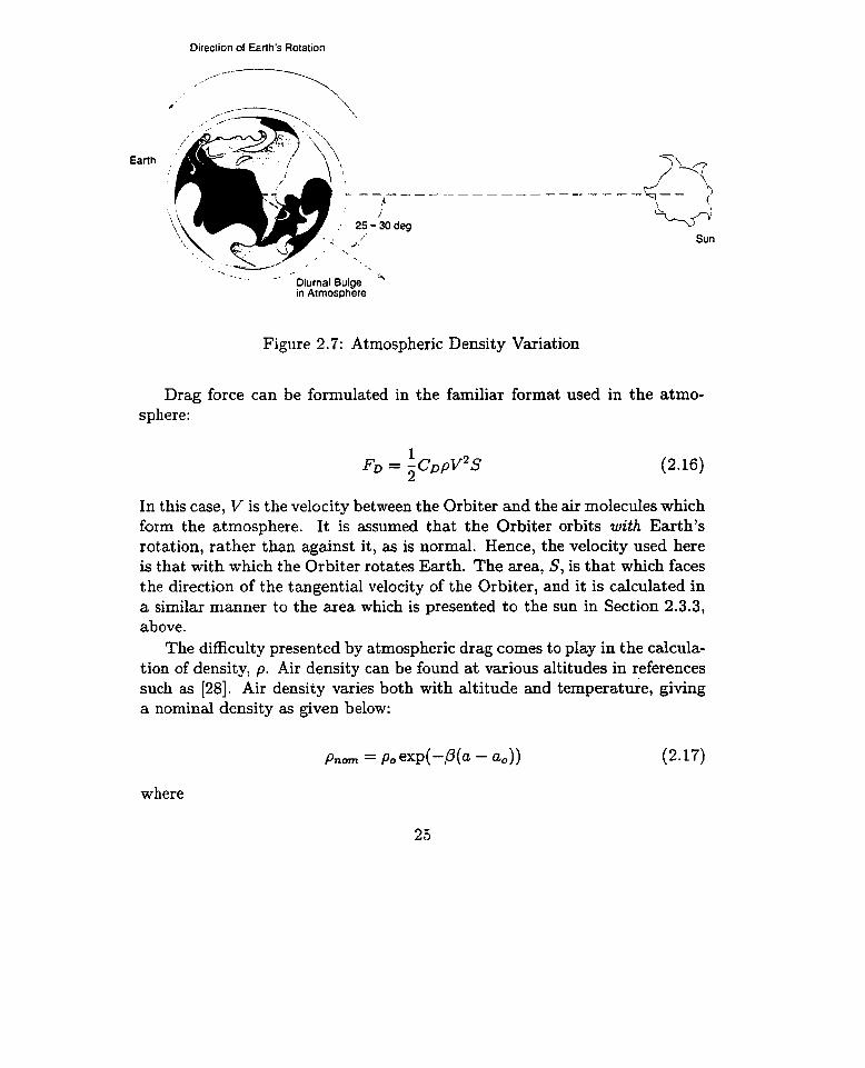
Figure 2.7: Atmospheric Density Variation

Drag force can be formulated in the familiar format used in the atmosphere:

In this case, V is the velocity between the Orbiter and the air molecules which form the atmosphere. It is assumed that the Orbiter orbits with Earth's rotation, rather than against it, as is normal. Hence, the velocity used here is that with which the Orbiter rotates Earth. The area, S, is that which faces the direction of the tangential velocity of the Orbiter, and it is calculated in a similar manner to the area which is presented to the sun in Section 2.3.3, above.

The difficulty presented by atmospheric drag comes to play in the calculation of density, p. Air density can be found at various altitudes in references such as [28]. Air density varies both with altitude and temperature, giving a nominal density as given below:

where

and where p, is the density measured at some reference altitude a,, sea level, for example. The R,,. used in this case is 0.28, as suggested in [IO].

The variation in temperature occurs due to what is c d e d the diurnal effect: the heating of atmosphere on the side of Earth exposed to the Sun. This heat causes the air to expand in volume and decrease in density, often by significant amounts. This diurnal bulge can be seen in Figure 2.7, and is actually offset from the direct Earth-Sun line by approximately 30 degrees (see reference [17]). This is due to the rotation of the atmosphere with Earth.

Hence, density can be calculated once the temperature variation in a given orbit is known.

Such information can be found in references such as [IO], for different latitudinal positions. As an example, the multiplicative values of the diurnal effect for a latitude of 30 degrees (where local solar time is given as hours from midnight) is reproduced below:

1 HOUTS fTOm Midnight Diurnal E#ect ut 30 deg lut. 1 .O68 1 .O53 1.043 1 .O38 1.037 1.040 1 .O49 1.069 1.097 1.133 1.172 1.208 1.238 1.258 1.266 1.263 1.251

Hence, the air density can be calculated as the nominal density, multiplied by the diurnal effect factors given in Table 2.2:

17 18 19 20 21 22 23

p = DizlrnalEf fed x p,, (2.19)

1.232 1.209 1.184 1.159 1.133 1.109 1.087

Finally, the value of CD must be calculated. According to [17], CD takes into account both the spacecraft shape and the type of molecular interaction of the atmospheric species with its surface. In its most aerodynamic position (nose in the direction of travel), the Orbiter is cited as having a coefficient of drag of 2.0 [36]. In its other orientations, however, the Orbiter acts mostly as a flat plate. For the purposes of a conservative estimate, the coefficient of drag is assumed to be 2.6 in these cases. However, this will also Vary with altitude, as the air flow changes from a more continuous flow at lower altitudes to a more molecular flow at higher ones.

As with solar radiation pressure, the force and torque is exerted by atmospheric drag on the Orbiter in the nominal orbit frarne. They must be transformed to the DICE frame of reference.

Table 2.2: Diumal Effect at 30 degrees latitude

2.3.5 Gravity Gradient T'orque

Like al1 other large spacecraft in orbit about a primary, the Space Shut- tle Orbiter experiences gravity gradient torque about its mass center. This torque is due to the fact that force due to gravity is not uniform, but varies according to an inverse-square relationship with distance separating the two bodies in question. In other words, there is a distinct gradient in the magnitude of the force exerted by gravity.

Gravity Field

Figure 2.8: Gravity Gradient Force on the Shuttle

Following the development in [22], one can see how the torque about the Orbiter shown in Figure 2.8 cornes about. In what follows, several assumptions are made. Specifically, only one primary, Earth, is considered to have influence; the mass distribution of Earth is assumed spherical; the Orbiter is considered a single body; and its size is considered small when compared to the distance from its m a s center to that of Earth. These assumptions lead to a formulation of torque due to the gravity gradient of:

This torque is measured in the body-fked frarne of the Orbiter. Note, from this equation, that 6 is perpendicular to l?,, and that, therefore, there can be no torque about the local vertical.

Following the substitutions made in [22], it can be shown that

where ~ 1 3 , ~ 2 3 , c33 are the direction cosines of the Orbiter axes with respect to the local vertical, defined by the unit vector

and 1, above, is given by the Orbiter's inertia matrix. If the principal axes of the Orbiter are selected as the reference frame,

the above formulation can thankfully be simplified to:

Note that one of the principal axes must be aligned with the local vertical in order for the gravity gradient torque to vanish. Thus, the tendency of such a torque will be to turn the Orbiter in order t o align its principal axes with the local vertical. This torque is exerted on the Orbiter in the nominal orbit frame of reference.

In order to solve this problem, an inertia matrix for the Orbiter must be determined (a nominal one is provided in Appendix B) and the altitude of the Orbiter must be known. The torque will be calculated in the frame of the Orbiter Fm (see Figure 2.1), and must be transformed to the DICE frame of reference Fd.

Chapter 3

Disturbance Forces in Simulation

The disturbance forces outlined in Chapter 2 are dependent on many factors: orbital altitude, Space Shuttle orientation, the mass and inertia of DICE, to name only a few. In addition, they are alrnost al1 dependent on each other, as they interact simultaneously on one system. In order to size these disturbances at different times and with different parameters, a simulation in XMath and SystemBuild was constructed. Simulations were run for the 7-minute run-time envisioned for controller and SI tests. In this way, it is possible to see how DICE will have to cope with different disturbance forces a t different times during its mission.

3.1 Apparent Forces

3.1.1 Forrnulat ion

Apparent forces are those forces which act on the Space Shuttle Orbiter, while DICE remains stationary in the orbital frarne of reference. From the discussion in Chapter 2, solar radiation pressure, atmospheric drag, and gravity gradient torque must al1 be classified as apparent forces.

These three different types of force were formulated in SystemBuild. Hardcopies of their block diagrams and supporting functions can be found in Appendix C. The parameters with which these forces vary were collected into one function (called 'set -parameters'), which is called prior to simulation

Figure 3.1: Shuttle in Orientation 1, Nose Forward, PBDs Away from Earth

Figure 3.2: Shuttle in Orientation 1, Nose Away Tom Eartb, PBDs Aft

as an initialization step. The very nature of these apparent forces, in that they act on the Or-

biter and not on DICE itself, demands that particular functions be created specifically for their needs. For instance, the atmospheric density must be calculated at a specific time in orbit, taking orbital altitude and diurnal effect into account, in order to allow the calculation of atmospheric drag. Functions such as these have been coded as MathScript blocks which cal1 functions during the simulation runtime. These functions can also be found in Appendix C.

In many instances, it is necessary to find the orientation of the Orbiter relative to the orbital frame. A nominal orbit is therefore specified at the outset by the user, and a MathScript function named 'orient' is used to find the orientation at which one would expect to find the Orbiter if it was following this nominal orbit exactly. To this is added the angular displacement caused by the disturbing torques which have acted on the Orbiter up to this point in time. Thus, a time-history of the Orbiter orientation emerges.

The 'orient' function allows the user to specify one of three different types of orbits:

Orientation 1: Earth pointing, in a standard configuration such as those shown in Figures 3.1 and 3.2, with the principal Orbiter axes aligned with the axes of the orbital frarne.

Orientation 2: Earth point ing in a non-standard configuration (Le., point-

ing along a user-specified vector in the Orbital frame)

Orientation 3: Pointing along a user-specified vector in the inertial frame (Sun-pointing, for example)

The surfaces of the Orbiter are referred to by number in many of the functions that are used to calculate the apparent forces. The nose is surface 1, the tail is surface 2, the Cargo Bay is surface 3, the belly is surface 4, and the two remaining identical sides are surfaces 5 and 6. These values correspond to the entries in Table 2.1.

The apparent forces on DICE have been formulated into a pre- pro- grammed simulation, both individually and collectively. Since these forces act on the Orbiter, and not on DICE, they are independent of DICE's position in the middeck. Therefore, they can be calculated 'ahead of time' and added to a full simulation of DICE during a controller or SI run.

3.1.2 Results

The following figures demonstrate how these apparent forces affect DICE, and how they differ when their parameters are varied.

Atmospheric Drag

Figures 3.3 to 3.6 demonstrate how Atmospheric Drag varies with altitude. The range of selected altitudes (200 km to 450 km) are those a t which the Orbiter generally flies. The accelerations, both linear and angular , which are displayed, are the accelerations of DICE as seen from the SVS fiame of reference. That is, the orientation of the axes corresponds to those of fiTS as seen in 2.2, and the origin is the 'nominal' or initial position of DICE in the middeck. As is to be expected, the magnitude of the accelerations decreases a t higher altitudes. The 'step' which appears in these figures is a result of diurnal effect. This effect has been implemented as it appeared in Table 2.2. In other words, the orbit has been divided into zones, each of which is kth of an orbit long. The diurnal effect is considered constant in each zone, and steps up or down to its new value when a new zone is entered.

In the atmospheric drag results shown, the accelerations are measured in SI units: the linear accelerations in 7 and the angular accelerations in 9. The Shuttle was in Orientation 1, nose forward, PBDs down for all r u s , and the Shuttle mass and inertia values found in Appendix B were used.

Figure 3.3: Atmospheric Drag at 200 km in Orientation 1




Solar Radiation

Figures 3.7 to 3.9 demonstrate how solar radiation pressure varies with orbital position. Once again, the graphs indicate the linear and angular accelerations of DICE as seen from the SVS frame of reference.

The orbital position variations are indicated on each figure with a starting time in seconds. That start time indicates the postion of the Orbiter with respect to the Sun. In other words, Figure 3.7 has a start time of O seconds, meaning that a t time = O s, the Orbiter is at the position in the orbit which is closest to the sun. At an orbital rate of 0.0012 radis (or 90 min/orbit), the Orbiter will cover an angular distance of 0.49 rad in the course of one 7-minute run.

In Figure 3.8, the start time is -1000 seconds, so the Orbiter initial position is 1000 seconds in the orbit before the closest point to the Sun. Interpret- ing this figure, it is obvious that the Orbiter changes position with respect to the Sun. While the solar radition flux from the Sun is always constant, the fact that the Orbiter presents different angles and surfaces to this flux as its orbit progresses accounts for the increasing and decreasing amounts of pressure along different axes.

Finally, in Figure 3.9, the effects of starting the Orbiter in the shadow of Earth's umbra can be seen. At approximately 320 seconds into the run, the Orbiter cornes out from behind Earth and experiences a distinct increase in radiation pressure.

In order to demonstrate how the forces on the Orbiter change during the orbit, the Orbiter has been oriented in a non-solar pointing orbit. Specifically, these results have the Orbiter in a nose-forward orientation (Orientation 1 from section 3.1.1). As for the atmospheric drag, the linear acceleration is expressed in 5 and the rotational acceleration is in 9.

Figure 3.7: Solar Radiation Pressure, Start Time = O sec

Figure 3.8: Solar Radiation Pressure, Start Time = -1000 sec

Figure 3.9: Solar Radiation Pressure, Start Time = -2000 sec

Gravity Gradient Torque

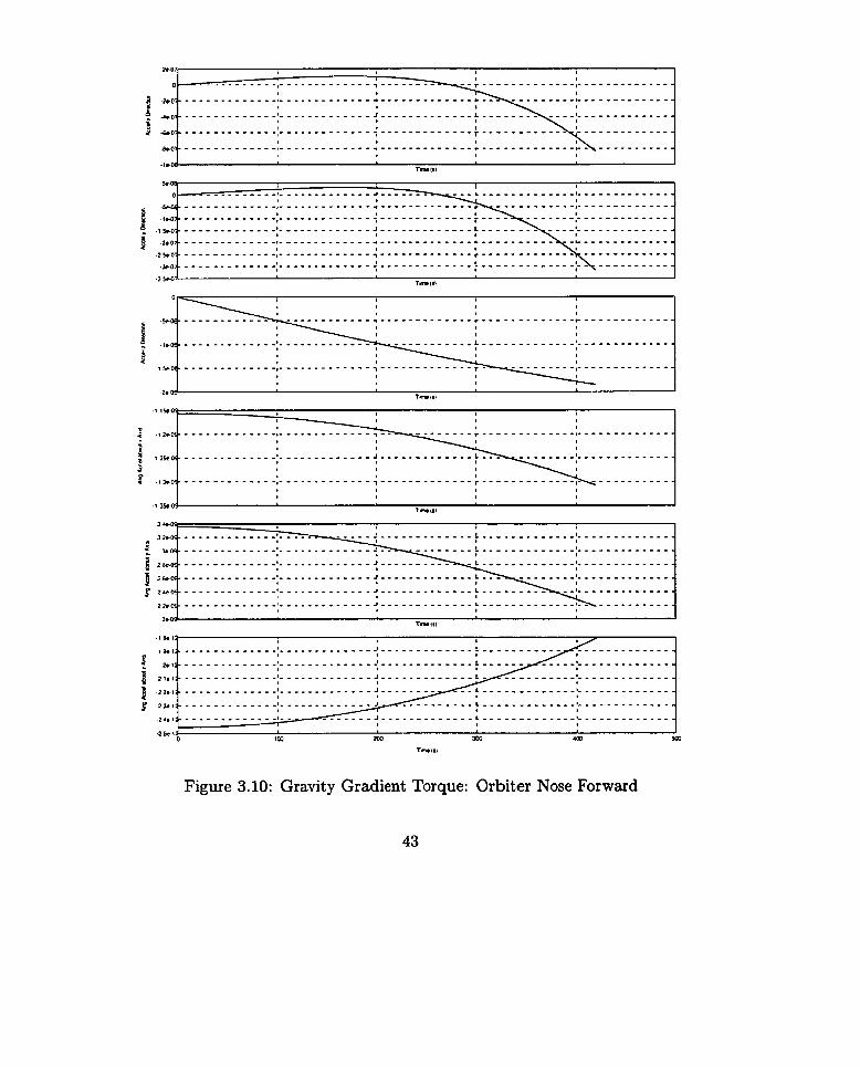
Figure 3.10 shows the gravity gradient torque for the Orbiter in the 'nose forward' orientation. Since the gravity gradient will tend to act in order to turn the Orbiter into a 'Payload Bay vertical' position (ie, nose toward Earth or away fiom it), this is the maximum amount of torque which can be expected to act on the Orbiter. The altitude of the orbit in the case shown in Figure 3.10 is 200 km. Once again, note that the linear accelerations are expressed in z, while the rotational accelerations are in 5.

- - - - - - - - - - - - -:- - - - - - - - - - - - -:--- - - - - - - ----; - - - - - - - - - - - - - ;\ - - - - - - - - - - 1 l I t

Tmi III

Figure 3.10: Gravity Gradient Torque: Orbiter Nose Forward

3.1.3 Total Orbiter Disturbances Finally, Figure 3.11 demonstrates al1 three of these apparent forces working together. This tirne, it is the total forces and torques acting on DICE in the SVS frame of reference which are displayed. The Orbiter is in the 'nose forward, PBDs up' position of Orientation 1, with an orbital start time of O seconds (indicating that the Orbiter is on the Sun- side of the Earth), and at an altitude of 200 km. These conditions should combine to give the worst case scenario for the Shuttle disturbance forces. Note that the forces are measured in Newtons, and the torques are in Nm.

Figure 3.11: Apparent Forces in Concert

3.2 Real Forces

3.2.1 Formulation

In addition to the apparent forces presented above, there are also forces acting directly on DICE. In this simulation, these are termed 'real', and are the two remaining sources of disturbance: the net acceleration of DICE fkom the Orbiter mass center due to orbital offset, and the force on DICE due t o the circulation of middeck cabin air.

The force due t o air circulation is calculated knowing the distance from DICE to the fan outlet, d, and calculating the force of the air ejected from a fan at that distance away. That force is calculated over the area of DICE. The air ejected from the fan is assumed to be a t a uniform speed at the nozzle exit, but the velocity spreads in a Gaussian distribution as air is entrained farther from the nozzle. The nozzle exit speed can be set in the 'set-parameters' file.

The manner in which the force is calculated can be seen in the System- Build block 'Fan Force-Torque' in Appendix C. The total jet force at the nozzle exit is calculated at the bottom left of the diagram, and this is multiplied by a weighing factor. (As the jet progresses towards DICE, it spreads over a larger area. The speed of the jet varies through the jet cross- section as a normal distribution. The amount and speed of the air that hits DICE is what makes up the weighing factor.)

The calculation of this weighing factor takes up the rest of block 'Fan Force-Torque'. Since this calculation is quite involved, many assumptions have been made to simplify it: DICE is assumed to be a circle of radius 0.1515 m, the center of mass is assumed to be located at the center of that disk, and the amount of air being blocked is often slightly overexaggerated. However, the effect of al1 these assumptions has been to overestirnate the forces on DICE. In other words, these forces represent the maximum forces possible.

In block 'Fan Force-Torque', the distance fiom the DICE mass center to the jet axis of symmetry is compared to the DICE radius. If it is less than the radius, most of the air jet impacts on DICE; if it is greater than the radius, less than half the air jet impacts on DICE. Using the standard deviation of the normal distribution, a fraction of the total jet area can be calculated. The normal distribution created by the jet is divided into 8 areas, and weighted according to how much jet force is produced in each area. This is represented by the cornparison and gain blocks, and the values were taken from (91. In

the case of most of the air impacting on DICE, one jet area is calculated, while in the case of less than half the air impacting on DICE, a smaller area is subtracted from the larger area in order to obtain the correct answer. In both cases, an exponential factor determines what angular fraction of the circular jet impacts on DICE.

Only the air circulation is a source of torque, since the orbital offset simply produces linear accelerations between the two m a s centers. A torque is exerted by the air jet if it is not centered on the DICE mass center. This torque occurs about the two axes perpendicular to the jet axis of symmetry. It is calculated by finding the moment arm between the jet axis and the DICE m a s center, and multiplying that by the force exerted on the exposed area of DICE. Note that this is not strictly correct. It is quite possible that DICE does not block the entire area of the jet. This possibility is taken into account in the calculated of the force exerted by the jet, but, in the case of torque, the centroid of the area DICE does block should be found. The moment arm would then be from this centroid to the DICE mass center. However, such a procedure complicates the calculations in an amount out of al1 proportion to the refinements in accuracy that it provides. Hence, it was not done.

Note that forces and torques caused by air circulation over the rib tip masses was ignored in this simulation, since this simulation concentrates on hub disturbances only.

The orbital offset formulation is a straight-forward application of the equations listed in Chapter 2.

Both these disturbances require knowledge of the position of DICE relative to the middeck walls. Hence, the simulation must be run in parallel with control or SI runs.

3.2.2 Results

The following figures show how DICE is dec ted by the real disturbances. Note that no control or SI runs were run in parallel with these results, and so DICE was assumed to be initially a t the origin (see Figure 2.2 for the origin coordinates), and to subsequently rnove only due to orbital offset and air circulation.

Orbital Offset

Figures 3.12 and 3.13 demonstrate how the acceleration due to orbital offset changes with Orbiter orientation. Figure 3.12 shows the acceleration when the Orbiter is in Orientation 1 with its 'nose forward', while the following figure shows it for the Orbiter in Orientation 1 with its 'nose up'. In each case, DICE is initially a t its origin in the middeck. Note that the 'nose up' position, which provides a greater vertical distance between the DICE mass center and that of the Orbiter, causes greater relative accelerations of DICE. This makes sense, because the two are in more different orbits than in the 'nose forward' case.

Figure 3.14 shows how the acceleration changes if the DICE bus is not centered with the center of the Orbiter. That center is represented by the Cargo Bay Center Line as defined in [5]. The acceleration that is now present in the y direction is sinusoidal, with a period of one orbit.

The forces shown here are in the SVS frame of reference. As always, the accelerations in these figures are in SI units: N for linear accelerations, and Nrn for rotational.

Figure 3.12: Orbital Offset Acceleration: Orbiter Nose Forward

Time (s)

Figure 3.13: Orbital Offset Acceleration: Orbiter Nose Up

Air Circulation

Figures 3.15 to 3.17 demonstrate the forces (in N) and torques (in Nm) exerted by air circulation on the DICE bus. Figure 3.15 demonstrates the force due to a single fan on the forward bulkhead. The jet axis of symmetry is offset from the DICE mass center, but the entire plume impinges on the DICE bus. This would be the largest force exerted on the bus. As seen fkom the figure, the largest force is approximately 0.0006 N. The results show several 'step' characteristics. This is an artifice introduced by the way that the DICE area affected by the air jet was modelled. In reality, the cuve would be smooth.

Figure 3.16 demonstrates the force due to a single fan on the aft bulkhead. The forces in this case are smaller, since the distance from the fan exit to DICE is greater. The forces are negative since they act along the negative z-axis in the SVS reference frame.

Finally, Figure 3.17 demonstrates how the magnitude of the force changes when fans are added to both bulkheads of the middeck.

The fan characteristics used in this simulation are those listed in the 'set-parameters' file shown in Appendix C. Note that the forces and torques are displayed in the SVS frame of reference.

Figure 3.15: Force due to Single Fan - Middeck Forward

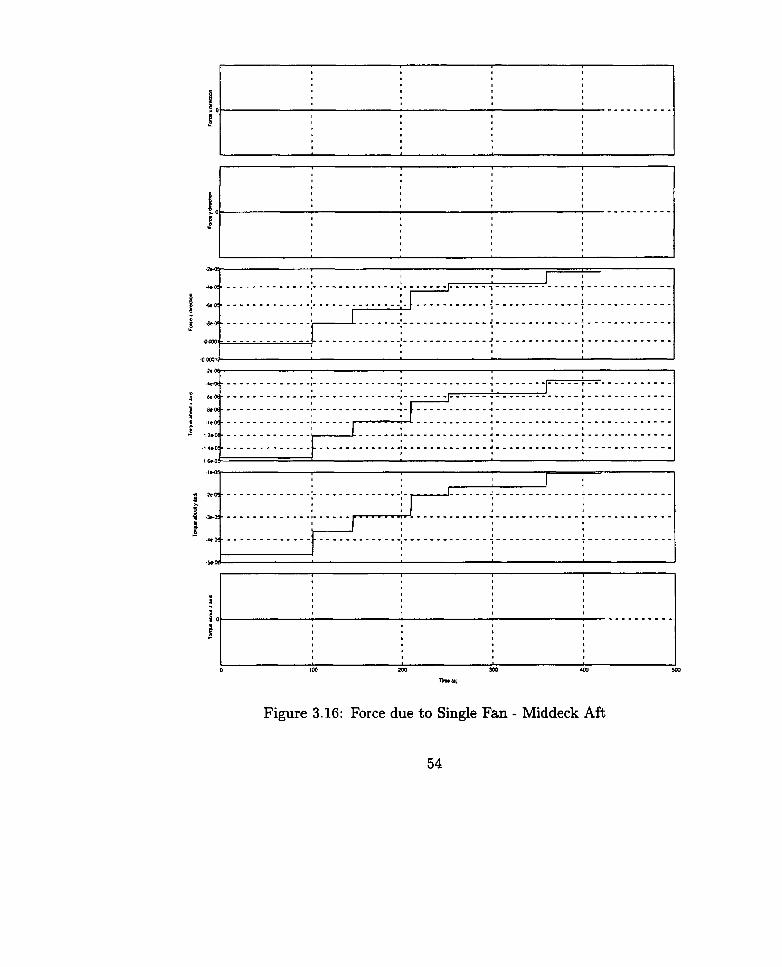
Figure 3.16: Force due t o Single Fan - Middeck Aft

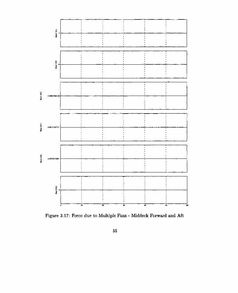
Figure 3.17: Force due to Multide Fans - Middeck Forward and Aft

3.2.3 Total DICE Hub Disturbances

Finally, Figure 3.18 shows these two effects - orbital offset and gravity gradient - acting in concert. As in previous figures, the forces are in N and the torques are in Nm. fn this simulation, the Orbiter is in the nose forwârd position, and fans are acting on both the forward and aft middeck walls. This would be the most disturbing environment for DICE as far as forces on its hub are concerned. In 3.18, these forces are seen from the SVS frame of reference, and the disturbances are clearly favouring particular axes. However, since DICE is turning in response to the torques exerted upon it, the thrusters will al1 require similar authority in order to react to these disturbances.

Figure 3.18: Real Disturbance Forces Acting in Concert (SVS Ftame)

3.3 Summary of the Simulation Results

Comparing Figures 3.18 and 3.11, it becomes clear that the forces acting directly on the DICE bus are greater than those acting on the Orbiter. The largest force in Figure 3.18 has a magnitude of 0.0005 N; the largest torque has a magnitude of 0.00016 Nm. These numbers seem reasonable, and also typical of the forces and torques seen in these simulations. Therefore, if they are rounded up to dlow for a margin of safety, i t can be seen that forces on the order of O(IO-~) and torques on the order of 0(10-~) will be exerted upon DICE.

It now falls to DICE to find a way to refute these disturbances.

Chapter 4

Air on the Move: Actuation

4.1 Design Requirement s

The requirements for the stationkeeping system as a whole drive the design of the actuators it uses. These requirements are fairly straight-forward and may seem obvious. However, it is essential that they be understood, in order to have the proper context to follow the forthcoming discussion. Hence, they are listed here for the reader's reference.

1. The stationkeeping system will be an integrated part of the DICE bus.

DICE must be stowed and deployed from middeck lockers on the Space Shuttle. The constraints on volume are numerous, and the stationkeeping system is therefore constrained to the DICE bus, a volume of approximately 0.3 m x 0.3 m x 0.15 m.

2. The stationkeeping system will provide thrust greater than that of the disturbances acting on DICE.

The disturbances acting on the DICE bus were detailed in Chapter 2. Recall that when middeck lockers are circulating air, that force was the greatest, exerting a force of O ( I O - ~ ) N. The actuators of the stationkeeping system must therefore be capable of exerting a force greater than this.

3. The stationkeeping system will provide additional torque for momen- turn dumping of reaction wheels.

In addition to providing torque to overcome DICE disturbances, the stationkeeping system must provide additional torque which will be used to 'dump' momentum fiom the reaction wheels. The reaction wheels will be on-board t o act as control experiment actuators - that is t o say, they will be used t o introduce known disturbances t o the system. Reaction wheels operate most efficiently around t heir zero-level, far from saturation, and the stationkeeping system must be capable of keeping the reaction wheek at this level. The exact impact of this requirement on the DICE design was not studied within the scope of this thesis, and it is recommended as a topic of further study.

4. The stationkeeping system will provide thrust less than NASA safety limits.

Since freeflyers are not a de rigeur presence on the Space Shuttle Or- biter middeck, it is difficult to guess what safety limits NASA will choose to impose on DICE. In order to get a ballpark idea, impact safety iimits used by Spar Aerospace in constructing its robotic arms for space applications in the Shuttle Payload Bay and the upcoming International Space Station were used. The 'runaway' impact energy of such a structure must not exceed 0.5 Joules 1121. Assuming DICE has a mass of 22.7 kg (or 50 lb), the speed of the freeflyer on impact could not exceed 0.21 m/s. Assuming DICE has 3.5 m of maximum runaway space in the middeck, this limits the acceleration t o 0.006m/s2. Hence, the net force exerted by DICE is limited to 0.14 N, or 0.07 N per thruster.

5. The stationkeeping system will not outgas foreign gases into the Or- biter.

In order to comply with NASA safety requirements (271, the stationkeeping system must not emit foreign gases into the Space Shuttle middeck.

6. The stationkeeping system will provide cooling to DICE interior electronics.

In addition to providing thrust to the DICE freeflyer, the stationkeep ing system will also cool DICE bus interior electronics so that they meet NASA temperature requirements, which specify that inaccessible

surfaces will not exceed 120 F, while external surface temperatures will not exceed 113 F. [2î] .

4.2 Design Characteristics

The concept of the system used for the actuators in the DICE stationkeeping system is deceptively simple. Air must be circulated inside the bus in order to cool the electronic equipment on-board. Instead of allowing that air to simply exit the bus, it is exhausted at strategic locations and angles to produce a net force or a net torque on DICE. In this way, one system, that of air recirculation, will perform two functions.

While the concept is simple, the implementation has not been so. The design of the DICE air system has undergone many design evolutions, each with its own benefits and drawbacks. The folfowing sections describe how that system was first conceptualized and implemented on the Integrated Prototype Model, and what design evolutions have been made since then. Chapter 5 will provide some details of how those two systems compare in practice.

4.2.1 Actuator Subsystems

The initial design of the DICE stationkeeping system was based on the theoretical predictions detailed in [18]. Using air as a source of propulsion would satisfy requirements 4 and 5 from section 4.1, since recirculated cabin air would be used to cool the electronics and provide a source of propulsion free of foreign contaminents. The air was to propel the DICE bus in order to provide both translational and rotational position control. In order to do this, the air system was designed to have three major subsystems: fans, plenum, and nozzles.

The design of the stationkeeping actuators is as follows: The fans drive the air through the bus, and, as such, are the largest

consumers of power in the air system. The fans operate on an on-going basis, providing a continua1 source of cool air to the DICE bus electronics. They are located in opposition on DICE (i.e., on opposite bus walls) in order to counter-balance each other and reduce the amount of net torque which is imparted to DICE by the rotation of the fan impeHors.

The air drawn in by the fans is pulled into a plenum, or pressure vessel. In this case, because the required thrust is so low, the pressure that is built up

in the plenum is equally low. The electronics that require cooling are located within the plenum, where air will circulate around them. The plenum's volume rnust therefore be quite a large fraction of the bus volume. Air is directed as required at the plenum entrance and exit using appropriate guide vanes.

When the air exits the plenum, it does so by way of several T- joint nozzIes. These nozzles are designed to provide a net thrust of zero unless thrust is desired. A valve in the nozzle controls the amount of air exitting each end, and can be calibrated to a zero-position appropriate for that nozzle. The nozzles are strategically located on the DICE bus so that, in sum, the nozzles provide thrust in the x- y- and z- directions, and torque about those same axes. Efforts are made to reduce the amount of exitting air which impacts on the flexible ribs.

4 - 2 2 Implementation on the IPM The Integrated Prototype Model served as the initial engineering mode1

for the DICE project, and, as such, has a scaled-down version of the air system installed. Since the IPM sits on air bearings and maneuvers in an almost frictionless manner on a flat table top, the IPM can only implement a two-dimensional version of the stationkeeping system. Two axial fans are mounted flush on opposite bus walls, and draw air into the upper level of the IPM. The entire upper level serves as the plenum in this case, with ducting leading to the nozzles. Two types of nozzle have been implemented: two identical exterior T-nozzles serve as the side thrusters, while a larger interior T-nozzle with extended ducting provides forward and backward thrust.

For specific details on the implementation of the air system on the Inte- grated Prototype Model, see the appropriate sections in 151 and [18].

4.2.3 Lessons Learned frorn the IPM The initial air system design was based on t heoretical considerations.

However , the construction of the IPM highlighted several poorly- understood design problems. Part of the requirements of this thesis was to examine these problems and suggest solutions to them.

The first was the overall layout of the stationkeeping system nozzles. The initial flight design had the thrusters aligned along three orthogonal axes al1 passing through the DICE center of mass. The third of these axes (passing

Figure Alternative Nozzle Positioning on DICE Bus

Figure 4.2: Proposed Nozzle Cluster

63

through DICE top to bottom, orthogonal to the plane of the ribs) was prob- lematic. Since these nozzles were not directly attached to the air plenum as were the nozzles on the other two axes, they would require significant ducting. As volume inside the DICE bus is at a premium, an increasing amount of ducting is not desirable. Also, the existence of these nozzles in their present position means that the bus does not possess a flat surface, which could be a concern for stowage. An alternative arrangement for nozzle positioning is shown in Figure 4.1, and the details of its design can be found in 1191. It provides a design symmetry which is aesthetically appealing, and a redundancy in certain directions. A more detailed view of a 'nozzle cluster' can be seen in Figure 4.2.

The second design problern was the choice of fans. According to [31], fans can be classified as propellor, axial, or centrifugal. It was found (see 1191) that axial fans, as used on the IPM, are primarily volume-flow devices, while centrifuga1 fans are pressure devices. In its present configuration, the stationkeeping system for DICE has been designed as a pressure system. The use of axial fans in such a situation is inefficient, particularly flush- rnounted as they have been on the IPM. Centrifuga1 fans corne in three shapes: backward-bladed (the blades are curved backward from the direction of rotation), radial-bladed, and forward-bladed (with the blades curved int O

the direction of rotation). Fan characteristics for these fans, as well as axial fans, can be seen in Figures 4.3 through 4.6, as taken from [4]. The backward- bladed fan is that which is generally used for low- pressure applications such as ours. Identification of the fan operating point is dependent on the interior bus layout and the air flow rate required.

The third design problem is closely related t o the second: the design of the fan system. The use of two counter-rotating fans in parallel is still anticipated, and Figure 4.7, reproduced from [31], shows how the system operating point is changed when considering fans in parallel. Figure 4.8, also from [31], shows the effect of changing the ambient air density on both the fan and the 'system', where the system here is the fan inlet, bus plenum, and the outlet nozzles. This is an important design consideration, since DICE will undoubtedly experience bot h nominal Space Shut tle cabin pressure (14.7 psi) and the pressure used when EVA activity is underway (10.2 psi).

The fourth design problem is that of designing an effective 'system' - that is, the air inlets, bus plenum, and nozzle outlets. A system consisting of fan inlets, ducting through electronics, two counter-rotating fans, an open plenum, and the outlet nozzle configuration suggested in Figure 4.1 was de-

5 T\ Pressure

Normal ~peratihg Range

Volume Flow

Figure 4.3: Performance Curves for Axial Flow Fan

Volume Flow

Figure 4.4: Performance Curves for Centrifuga1 Backward-Bladed Fan

Volume Flow

Figure 4.5: Performance Curves for Centrifuga1 Radial-Bladed Fan

Volume Flow

Figure 4.6: Performance Curves for Centrifugal Forward-Bladed Fan

Volume Flow

Figure 4.7: Operation of Two Identical Fans in Parallel (Dashed Line Represents the Fan System at a Particular Operating Point)

.' System Operaiion Fan Pressure 1

i

Volume Flow

Figure 4.8: Effect of Change of Ambient Air Density on Fan and System

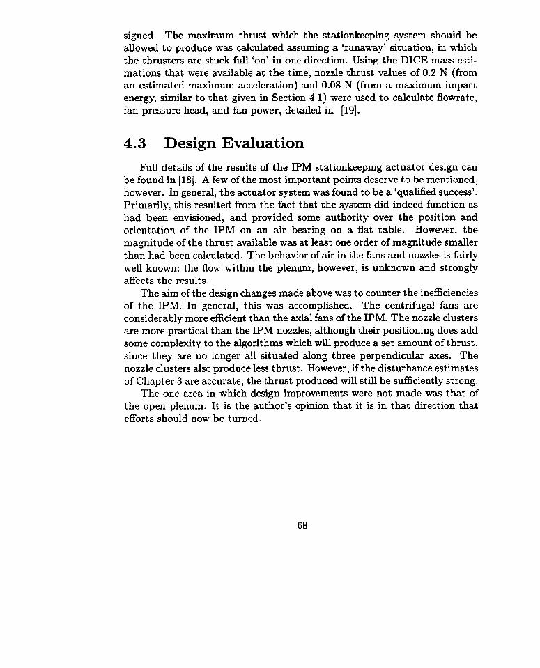
signed. The maximum thrust which the stationkeeping system shouid be allowed to produce was cdculated assuming a 'runaway' situation, in which the thrusters are stuck full 'on' in one direction. Using the DICE mass esti- mations that were available at the time, nozzle thrust values of 0.2 N (from an estimated maximum acceleration) and 0.08 N (from a maximum impact energy, similar to that given in Section 4.1) were used to calculate flowrate, fan pressure head, and fan power, detailed in [19].

4.3 Design Evaluation

Full details of the results of the IPM stationkeeping actuator design can be found in (181. A few of the most important points deserve to be mentioned, however. In general, the actuator system was found to be a 'qualified success'. Primarily, this resulted from the fact that the system did indeed function as had been envisioned, and provided some authority over the position and orientation of the IPM on an air bearing on a flat table. However, the magnitude of the thrust available was at least one order of magnitude srnaller than had been calculated. The behavior of air in the fans and nozzles is fairly well known; the flow within the plenum, however, is unknown and strongly affects the results.

The aim of the design changes made above was to counter the inefficiencies of the IPM. In general, this was accomplished. The centrifuga1 fans are considerably more efficient than the axial fans of the IPM. The nozzle clusters are more practical than the IPM nozzles, although their positioning does add some complexity to the algorithms which will produce a set amount of thrust, since they are no longer al1 situated along three perpendicular axes. The nozzle clusters also produce less thrust. However, if the disturbance estimates of Chapter 3 are accurate, the thrust produced will still be sufficiently strong.

The one area in which design improvements were not made was that of the open plenum. It is the author's opinion that it is in that direction that efforts should now be turned.

Chapter 5

Stationkeeping Put to the Test

Much of the foregoing discussion has been theoretical or cornputational in nature. These methods of attacking the stationkeeping problem have been essential for the development of a suitable stationkeeping system. It is now time to take that systern out of the theoretical world and put it t o the test. This involves building a hardware model of the system and taking meaçurements of the system as it would be constructed. The importance of doing so cannot be overexaggerated. Building a hardware model effectively tests al1 the assumptions made during the design process. It points out errors and interactions which are not obvious on paper, but which greatly affect the performance of the system in actualization. Finally, it demonstrates to the designer the difficulties, limitations, and possibilities of the system.

This chapter will present the results of tests made on both the Integrated Prototype Mode1 and a new, more evolved model of the DICE bus, and, thus, will evaluate the performance of the stationkeeping system.

5.1 A Forum for Verification

The design of a stationkeeping system for DICE has been based on many assumptions of the system's performance. For instance, certain friction losses inside the DICE hub were assumed (see [18] for further elaboration). While these assumptions were necessary in the initial conceptual phase of the DICE project , they must be checked against reality, in order to confirm their validity for the problern in question.

The aim of the IPM was to resolve the question of whether design as-

surnptions made in the conceptual stage of the DICE project were valid. While the IPM did resolve this question in some areas, it was unsuccessful in others due to the rapidly evolving flight design. The IPM was unable to adapt to match the design on paper. Measurements made on the IPM could be used as representative or "ballpark" measurements, but they codd not be used to characterize the stationkeeping system for the flight model. This was principally due to the IPM design problem solutions that were presented in Chapter 4: a new t hruster design, a different fan selection, and an alternative layout of the interior volume.

It was decided that a completely new mock-up of the current DICE design should be created, in order to test the performance of the stationkeeping system. The design of this mock-up was based on drawings of the most recent DICE hub design by Dynacon Enterprises Ltd. The primary goal of the mock-up was to mimic, as closely as possible, the interior volume of the DICE hub, as well as the stationkeeping system. This way, the effectiveness of the stationkeeping system actuators could be verified in the situation for which it was designed.

5.2 Bus Mock-up Design and Construction

The Bus Mock-up, as it becarne known, is shown below in Figures 5.1 and 5.2, taken from [32]. Figure 5.2 is an interior view, and shows the ceiling of the Bus Mock-up, to which most of the interior elements are attached.

The Bus Mock-up outer shell was constructed out of dark plexiglas, sized to match the interna1 volume of the DICE flight model, as shown in Figure 5.3. The interior elements, including rate sensors, reaction wheels, and computer boards, were modelled out of styrofoarn, and were accurate in shape and size only. That is to say, they contained no mechanical elements. The thrusters were also modelled for size and shape, and did not include motorized servos to dictate valve position. In fact, only one thruster set was equipped with a directional valve which could be used to direct airflow. Centrifuga1 fans were operated at what were envisioned to be normal operating conditions.

The Bus Mock-up, as a facility, can be used to answer many questions about the DICE design. In particular, tests on such a facility could obtain the following results:

The relationship of nozzle thrust with respect to thruster valve angle

Figure 5.1: The Bus Mock-up, Exterior View

Figure 5.2: The Bus Mock-up, Interior View with Selected Components

Figure 5.3: Bus Mock-Up Specifications

r The relationship of thrust with respect to time (i.e., are there any time variations to the flow?)

A velocity profile of flow (for both nozzles of a thruster)

The torque and/or force induced on DICE by valve movements in the thruster

Whether coupling between thrusters due to internal flow variations occurs

Power consumption properties

r The effect of pressure scaling

r Patterns of internal flow

While it does not fa11 within the scope of this thesis to answer al1 these questions, many of them are quite important, and deserve careful scrutiny. In particular, examining the power consumption of the entire stationkeeping system and introducing variablity in the ambient pressure are two areas of study deemed crucial, but will not be covered in the following sections. They have been recommended for further study at the end of this document.

5.3 Test Results

5.3.1 Preliminary IPM Tests

As an exercise in familiarization with the apparatus, and also as a characterization of the early design, air flow tests were first performed on the In- tergrated Prototype Mode1 before applying them to the Bus Mock-up. Data gathered during this IPM procedure could then be compared with compara- ble data gathered from tests made on the Bus Mock-up. It was hoped that such a procedure would allow one to see the effect of the design changes which had occured between the two models. It was also felt that the data from the Bus Mock-up would not be nearly so illuminating, if there was nothing with which to compare it.

Support

Figure 5.4: Apparatus for Air Flow Tests

Procedure and Results

The aim of the tests performed on the IPM were to accumulate experience with the equipment, and to form a baseline against which further tests on the Bus Mock-up could be compared. Therefore, the tests which where performed were the following:

A characterization of the flow field exitting both nozzles on one side thruster

a A characterization of the air fiow from the larger thruster

0 A cornparison of mid-stream air flows a t different valve angles

A low-speed manometer, contributed by Dr. J. D. DeLaurier, was used to make the flow characterizations, while a force balance was used t o make

Travarsal Disiance (cm)

' 8 C--*-----< I .

4 0 20 0 0

Figure 5.5: Thruster and Nozzle System in IPM Interior

the force measurements. Use of such apparatus in the measurement of air velocities and forces exerted by a free jet is common, and specific references and details cari be found in [25] and [33]. A vice was used to regulate the distance between measurement points. The complete apparatus is shown in Figure 5.4.

Figure 5.5 shows how air is regulated in the thrusters on the IPM. A wedge slides back and forth in the thruster in order to regulate the amount of air each side will receive. The wedge traverses a total distance of 4.0 cm. Thus, when the wedge is centered between the two sides, its position is 2.0 cm. When it is full to the right, its value is 0.0 cm; when it is full to the left, its value is 4.0 cm.

The results of each of the experiments themselves can be found on the following pages. Figures 5.6 and 5.7 show the pressure and velocity profiles, respectively, of both the right and left nozzles of one side thruster, when the wedge is in its neutral position. Note that the horizontal distance is measured in centimeters, and increases as the bus wall is approached. The interior diameter of the IPM side thruster nozzles is 3.3 cm.

The particularly striking feature of these profiles is their asymmetry. The same quality is evident in Figure 5.8, in which pressure and velocity profiles of the main thruster are shown. The asymmetry indicates that the air is 'hugging' the outside wall of the thruster nozzle, to the extent that a slight suction or recirculation area is created on the inside thruster wall. It is interesting that this feature is as prominent for the main thruster as for the side ones, since it was the author's intuition that the long duct after

Right Side Thruster - IPM

20

Vertical Distance (cm) Horizontal Distance (cm) Left Side Thruster - IPM

Vertical Distance (cm) Horizontal Distance (cm)

Figure 5.6: Pressure Profiles of the Side IPM Thrusters

Right Side Thruster - IPM

Vertical Distance (cm) Horizontal Distance (cm) Left Side Thruster - IPM


Figure 5.7: Velocity Profiles of Side IPM Thrusters

the turning wedge in the main thruster system would smooth the flow more evenly throughout the nozzle area. This intuition would appear to be in error, assuming it is not a simple case of inadequate duct length.

The air velocity £rom each thruster can be seen to be quite high, with a maximum in the neighborhood of 10 m/s. The maximum velocity of the side thrusters is a factor of two higher than that of the main thruster. Since the area of the side thrusters is lower than that of the main thruster by approximately a factor of two, it can be surmised (referring to equation (2.1)), that the flow rate is the same through each type of thruster.

In Figure 5.9, a series of pressure profiles have been cornpiled, where each profile is taken at the same vertical height on the thruster, but at a different wedge position. The general trend is of decreased dynamic air pressure as the wedge position is decreased, the expected outcome. Note that the changes in pressure occur only in the peaking pressure section, and not in the suction section of the curves. This provides further evidence that the majority of the air is hugging the outer circumference of the thruster nozzle, rat her than smoothing out and using the full thruster area.

Sources of Error

The sources of error in the manometer measurements are easy to enu- merate. The most predictable error is the reading error, which is dependent on the scale of the measurements taken. In this case, the scale was in mil- limeters, and the reading error consists of f 0.25 mm, which translates to an uncertainty in the velocity of 0.06 m/s. While the low-speed manometer has been constructed with a time lag in order to smooth out the influence of turbulence, some variability in the readings was noticed a t some data points nonetheless. The maximum value of this variability was & 1.5 mm, or f 0.37 m/s.

In addition to these quantitative sources of error, there were some which could not be quantified so easily. Because the manometer has a significant time lag, it took quite some time for the height of the liquid in the manometer t o achieve a steady-state value. The rate of change of the liquid height could be quite slow in some cases. Due to this efFect, it is possible that some measurements were taken prematurely, before the liquid height had achieved its true steady-state value. h t h e r errors could evolve from the lack of correct positioning of the pitot tube, parallel to the direction of the flow, possible inaccuracies made in the height of the pitot tube during a

Main Thruster - IPM

Vertical Distance (cm) Horizontal Distance (cm) Main Thruster - IPM


Figure 5.8: Pressure and Velocity Profiles of IPM Main Thruster

Air Pressure at Various Wedge Angles for IPM Thrusters 90 1 1 1 1

+++ Wedge Position 0.0 cm --- Wedge Position 1 .O cm -.- Wedge Position 2.0 cm . . . . Wedge Position 3.0 cm - Wedge Position 4.0 cm

1 O 15 Horizontal Position

Figure 5.9: Pressure Profiles at Different IPM Wedge Angles (Horizontal Position of 25 Equally Distributed Points = 3.3 cm Diameter)

single traverse of the air jet, and the evaporation of the alcohol used in the manometer, since the manometer cannot be sealed to the atmosphere.

5.3.2 Bus Mock-up Tests

Actuator Airflow Test Procedure and Itesults

The tests which were performed on the Bus Mock-up closely ressembled those performed on the IPM. Both flow characterizations and force measurements were made. The measurements made in this case inchded:

A characterization of the flow field exitting both nozzles on one thruster

O A comparison of mid-stream air flows at different valve positions

0 A comparison of the 12 nozzle force values with the bus empty

0 A comparison of the 12 nozzle force values with the bus full

0 A compilation of thrust vs. valve position measurements

0 Observations of the time-varying nature of force meaçurements

The measurements made on the Bus Mock-up occured a t several inter- vals. Initially, the Bus Mock-up was kept empty, similar to the interior state of the IPM. In this way, measurements could be made and reasonable con- clusions could be drawn concerning the distribution of air inside the bus. Meaçurements were also made with al1 the interior components correctly sized and fitted into place. 'Before' and 'after' measurements of this nature demonstrate the energy dissipation introduced by the interior elements.

One of the thruster nozzles on the Bus Mock-up was equipped with a wedge valve similar to that which was used in the IPM thrusters. Its total traverse length was 5.0 cm. Hence, it's neutral position was located a t 2.5 cm.

Figures 5.10 and 5. I l show the air pressure and air velocity profiles for both the right and left nozzles of one thruster. The abbreviation BMU which appears on the graphs stands for Bus Mock-up. In order to compare these results with those obtained for the IPM, the profiles were taken with the Bus Mock-up empty of components. Note that the pressures and velocities are significantly smaller than those seen in Figures 5.5 and 5.6 for the IPM.

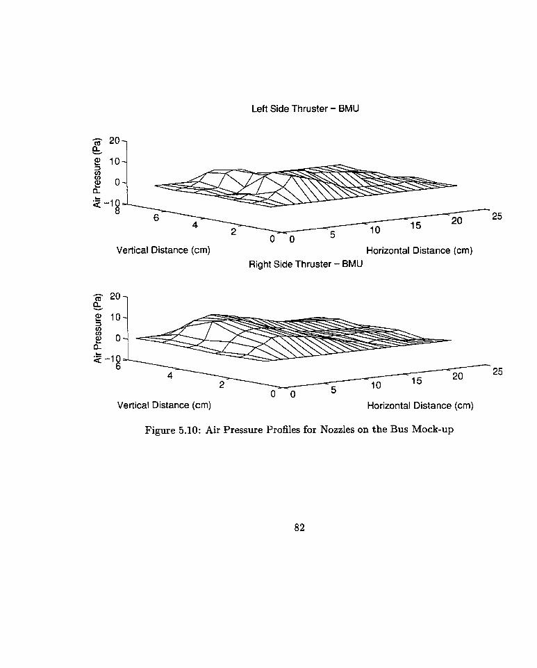
Left Side Thruster - BMU

Vertical Distance (cm) Horizontal Distance (cm) Right Side Thruster - BMU

- 20 25


Figure 5.10: Air Pressure Profiles for Nozzles on the Bus Mock-up

Left Side Thruster - BMU

Vertical Distance (cm) Horizontal Distance (cm) Right Side Thruster - BMU


Figure 5.11: Air Velocity Profiles for Nozzles on the Bus Mock-up

In order t o measure the force exerted by each thruster, a scale was placed perpendicular to the flow, from which it measured the force in grams. This value was converted to kilograms, and a gravitational constant of 9.8 m/s2 was used to convert this t o Newtons. Complete reflection of the air from the surface of the scale was assumed as a worst case, so d l force values were divided by two. Additionally, care was taken to make sure that the entire air flow impacted on the scale by placing it five centimeters from the mouth of the thruster.

Figure 5.12 shows the thrust values of al1 12 nozzles, when the bus is both empty and full. The plots show the nozzles grouped into 4 categories of 3 nozzles. This grouping was done simply to clmiS. the results. Each of the categories represents a nozzle direction, and, in 5.12, the first is down, the second is up, the third is left, and the fourth is right. The number at each data point is simply an identification of that nozzle. The figures were plotted this way in order to make obvious certain trends among like-pointing nozzles. Note, for example, that , when the bus is empty, the vertically pointing nozzles are considerably stronger than the horizontally pointing ones. When the bus is full, no particular direction seems favored over the others, as the air is dissipated more randomly about the interior.

Overall, the effect of filling the bus is the depression of the thrust exerted a t the nozzles. An average drop of approximately 30% is seen in the case where the interior components are installed. This leads us to believe that, in its present configuration, the interior components of the bus dissipate a considerable fraction of the energy injected into the system by the fans.

Figure 5.13 gives us a very important result: the maximum value of force which can be obtained by turning a thruster 'full on'. This maximum value can be read off the graph to be 0.0094 N, or approximately 0.01 N when ease of calculation is desired.

The information in Figure 5.13 is also helpful in modelling the stationkeeping actuators. It is interesting t o note that the relationship is almost linear, until the very extremes of the valve position are reached. One could postulate that a certain area threshold exists, below which the resistance incurred through wall friction would be high enough to discourage air flow through that region. If a sirnilar plateau existed at the top end of the scale, it would support this argument. However, the results of Figure 5.13 are ambi- gious in this case, as the deviation of the b a l point from a linear relationship could be due to simple experimental error.

Finally, Figure 5.14 shows the variation of air pressure with wedge posi-

Figure 5.12: Thrust Distribution Amoung Bus Mock-up Nozzles

Thrust vs. Valve Position with BMU Full

Valve Position (cm)

Figure 5.13: Thrust vs. Valve Position for Bus Mock-up

Air Pressure at Various Wedge Angles for BMU Thrusters 12[ 1 1 1 1

"' Wedge Position 0.0 cm + --- Wedge Position 1 .O cm

+ -.- Wedge Position 2.0 cm . . . . Wedge Position 3.0 cm +++ Wedge Position 4.0 cm - Wedge Position 5.0 cm

\ +

-4 I 1 1 I I O 5 10 15 20 25

Horizontal Position

Figure 5.14: Air Pressure at Various Wedge Angles for Bus Mock-up (Horizontal Position of 25 Equally Distributed Points = 4.0 cm Diameter)

tion. The observations show similar trends to that which was observed on the similar experiments involving the IPM wedge.

Time variations of the force data where observed in al1 cases. This variation showed considerable jitter, and varied quite randomly up or down from some average value. In general, this introduced an error of f: 0.0007 N to al1 the results taken. I t can be presumed from this observation that the system had some difficulty in establishing steady flow inside the bus.

Sources of Error

The sources of error for the tests made on the IPM are al1 equally valid for the Bus Mock-up. In addition, the Bus Mock-up suffers from possible modelling errors, include machining inaccuracy, inaccurately sized interior elements, and incorrectly constructed thruster nozzies. The wedges used

to control air flow in the nozzles are also possible error sources, as they may have been inaccurately positioned with respect to the air fiow. Al1 force measurements were subject to a f 0.0005 N measurement error due to the accuracy of the measuring instrument, as well as the f: 0.0007 N time- variancy introduced above.

Airfiow Observations

When the tests for the Bus Mock-up were begun, the plans shown in Figures 5.1 and 5.2 were strictly adhered to. However, it was soon seen that these plans, while well-executed to meet volume and operational constraints, had some shortcomings from an airflow point of view.

Fan-Thruster Interaction The most apparent problem was that of the placement of the fans with respect to the 'corner thrusters', thruster sets 2 and 3. Because the fans and corner thrusters were too closely positioned, the air ejected from these thrusters was being pulled into fan inlets.

The problem 2s not that momentum is robbed from the system. Indeed, the thrusters irnpart a force on DICE, not by ejecting that air into the cabin, but by turning it with an internal wedge or valve. The force that is imparted on that turning wedge is transrnitted to the DICE bus as a whole. Since that wedge is internal to the thruster, it is unafkcted by the recirculation area at the fan inlet.

Rather, the problem is one of calibration. Because the fans create a low pressure region, they are actively 'pulling' air from one side of the thruster. Thus, when the internal turning wedge is in its center or neutral position, the air ejected from the thruster nozzle on the fan side is significantly more than that ejected from the opposite nozzle. The wedge would have to be moved significantly over to one side in order to achieve a net force of zero from the thruster. It would be possible to do this as a form of calibration. However, doing so would be undesirable. I t would lirnit the amount of authority the controller would have over the thrust produced by that thruster in one direction. The distance through which the wedge would travel in order to go from its neutral position to its 'full on' position would be significantly greater on one side and less on the other.

Air recirculation seemed significantly reduced by moving the horizonal nozzles (Nozzles 3 and 4) off center from the fan. This was accomplished simply by flipping the thuster set upsidedown. However, it was seen when

thread was attached to the outside of the horizontal nozzles, that some recirculation still took place. The best solution in this case would be moving the fans so that they are positioned in the corners opposite the corner thrusters.

There is also an additional problem associated with the close positioning of fans and corner thrusters. This problem is internal. When nothing inter- venes between them (and in Figure 5.2, nothing does), the air from the fans is blasted directly into the inlets of the corner thrusters. Therefore, these corner thrusters are favoured over the third thuster, which has Iess air %ow and, therefore, less t hrust.

When baffles were added to the Bus Mock-up, a marked change was seen. These baffles were simply cardboard rectangles which spanned the height of the mock-up and completely blocked the flow between the fans and the corner thrusters. (Note t hat al1 observations documented in this chapter were taken with t hese baffles installed.) The thrust from the corner thrusters decreased; that of the third thruster increased. Unfortunately, the third thruster was now slightly favoured over the two corner thrusters. Therefore, it is obviously necessary, not only to install baWes between the fans and the thrusters, but to provide more guidance to the air flow in order to distribute it evenly within the bus.

Interior airflow By attaching threads at various points inside the bus, a general qualitative view of the air circulation was achieved. In general, it was seen that the air circulation inside the bus was quite good. Some features of note are described below.

Information about air circulation around the computer was the most anticipated. Since a computer board spans almost the entire height of the Bus Mock-up, it was doubted that air would actually enter to circulate between the boards. For the most part, this suspicion was confirmed. The air tended to circulate over, under, and around the computer, but did not circulate well between the boards. Some slight agitation of the threads between the boards was seen, however, and it is possible that with a little bit of guidance, enough air could be diverted to cool the computer boards properly.

A similar situation was seen with the Vision, Rate Sensor Filter, and Health Monitoring boards - air circulation around the boards was good, but there was no circulation between them.

As was remarked above, the baffles blocked off the air flow between the fans and the corner thrusters. This was confirmed through observation.

There was extreme agitation of threads in areas where the baffles didn't block the flow, while the agitation behind these b d e s a t the inlet of the corner thrusters was much more subdued.

Finally, it was seen that, in the vicinity of the reaction wheels, the heat sinks tended to direct the air flow. Often, this meant that some heat sinks were directly in the air flow, while others were blocked from it. Such a situation will result in uneven cooling of the reaction wheel apparatus. If this causes a problem, it could be fked by adding air fiow guides in the volume around the reaction wheel.

Overall, it was seen that the air circulation in the bus was quite vigourous. Most elements are cooled directly by the recirculating air, and those which are not could be, if some small efforts were made at guiding the air inside the bus.

5.4 Actuator Modelling

5.4.1 Trends in Empirical Results

Figure 5.13 demonstrates the empirical force vs. valve position relationship for a single nozzle. For modelling purposes, this relationship is a slightly nonlinear one, with a slope close to 0.002 N/cm. The magnitude of the force fluxuation is approximately 10% of the total value, and appears to have an average frequency of 0.06 Hz. Some higher frequency jitter of a lower magnitude was also present.

5 A . 2 Simulation Modelling of Actuators

In order to model an air thruster actuator, the above information about the nozzle must be incorporated with information about the motor. The reaction between the re-positioning of the valve and the change in thrust is quite fast, demonstrating very little time lag. The motor characteristics must include a function for the conversion of the input signal (nominally voltage) into an angle on the motor shaft. Finally, gears, if they exist, must be included in the model.

Therefore, the mode1 of the actuator, assuming a steady plenum pressure, consists of these elements: a motor relationship relating input signal to shaft angle, a gear relationship relating shaft angle to valve position, a time lag

Figure 5.15: Location of Thrusters in DICE Rame of Reference

with a very low time constant, and the force vs. valve position relationship. This signal must be added to a noise signal of the magnitude and frequency given by the empirical results, above.

This is exactly what was done in order to model the air thrusters. Dia- grams of an air thruster model created in XMath Systembuild can be found in Appendix E. Inputs to this model are the motor voltage and a calibration factor; the output is the net force exerted by the thruster. Due to uncertainty about the motor to be used, the relationship between the motor speed and the voltage is left as a variable, located in the initial 'set-parameters' file. Some effort was made to model motor friction, and the slightly nonlinear relationship between the force exerted and the valve angle is included for higher fidelity. Note that this nonlinearity has been included in the model as it was observed during the Bus Mock- up tests. Therefore, it is iacluded as a seperate factor on each nozzle, and the nozzle forces are added together to get a net force. Hard stops also appear, in order to limit the distance the valve can traverse in the nozzle. The input to the air thruster is a voltage, and the output is the net thrust exerted by that thruster.

In order t o see how the forces exerted by one air thruster affect the DICE bus as a whole, the 'Stationkeeping System' was also modelled, and the

SystemBuild representation of this can also be seen in Appendix E. The inputs to this system are a unit vector (a vector of ones of the same size as the time vector), and the desired forces in the 3 principle directions and the torques about the 3 principle axes. An assumption has been made in order to distribute the six inputs arnong the thrusters, that assumption being that each of the voltage inputs to the air thruster models will be derived assuming maximum use is be made of each thruster. Six individual thruster blocks represent the actuators themselves. A calibration term can be set for each in the 'set-parameters' file. The noise or 'jitter' observed during the Bus Mock-up tests has been included at this level, so that the six thrusters will each have an independent noise source. Finally, the net thrust from each t hrust er is combined with the others, according to the following equat ions:

These equations were derived by assuming a 3-cluster thruster arrangement, identical to that which was used on the Bus Mock-up. Figure 5.15 shows where these thrusters are located in the DICE frame of reference. The origin (0,O) of the DICE frame is located at the geometric center of the bus. The first cluster exerts FI and F4, is located on the x-axis, and has the coordinates (9.5,0,0) with respect to the geometric center when viewed from the top. The two other clusters are located on the opposite corners of the DICE bus. They exert forces F2 and F5, and forces F3 and F6, respectively. Their coordinates are (-6.6,8.4,0) and (- 6.6,-8.4,O). Note that this assumes that the DICE mass center coincides with the geometric center of the bus. The coordinates correspond with those presently used by Dynacon Enterprises in t heir design.

5.4.3 Controlling the Actuators As stated in Chapter 1, a stationkeeping system consists of sensing devices, actuating devices, and control algorithrns that link the two. The majority

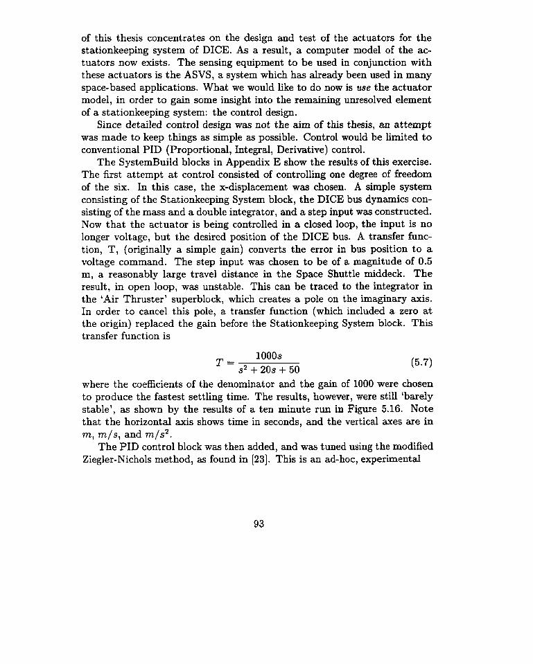
of this thesis concentrates on the design and test of the actuators for the stationkeeping system of DICE. As a result, a computer model of the actuators now exists. The sensing equipment to be used in conjunction with these actuators is the ASVS, a system which has already been used in many space-based applications. What we would like to do now is use the actuator model, in order to gain some insight into the remaining unresolved element of a st at ionkeeping system: the control design.

Since detailed control design was not the aim of this thesis, an attempt was made to keep things as simple as possible. Control would be limited to conventional PID (Proportional, Integral, Derivative) control.

The SystemBuild blocks in Appendix E show the results of this exercise. The first attempt a t control consisted of controlling one degree of freedom of the six. In this case, the x-displacement was chosen. A simple system consisting of the Stationkeeping System block, the DICE bus dynamics consisting of the mass and a double integrator, and a step input was constructed. Now that the actuator is being controlled in a closed loop, the input is no longer voltage, but the desired position of the DICE bus. A transfer function, T, (originally a simple gain) converts the error in bus position to a voltage command. The step input was chosen to be of a magnitude of 0.5 m, a reasonably large travel distance in the Space Shuttle middeck. The result, in open loop, was unstable. This can be traced to the integrator in the 'Air Thruster' superblock, which creates a pole on the imaginary axis. In order to cancel this pole, a transfer function (which included a zero a t the origin) replaced the gain before the Stationkeeping System block. This transfer function is

where the coefficients of the denominator and the gain of 1000 were chosen to produce the fastest settling time. The results, however, were still 'barely stable', as shown by the results of a ten minute run in Figure 5.16. Note that the horizontal axis shows time in seconds, and the vertical axes are in m, m/s, and m/s2 .

The PID control block was then added, and was tuned using the modified Ziegler-Nichols method, as found in (231. This is an ad-hoc, experimental

Figure 5.16: Results of Step Input without PID Control

method, and it produced coefficients of

The results of the the tuning can be see in Figure 5.17. A trade-off was necessary between overshoot and settling time. In order to be overly cautious, it was decided that, in this exercise, the overshoot wcruld be minimized, and the settling time would be sacrificed. This approach would maintain the DICE bus close to its desired position, but would limit its response time. As can be seen in Figure 5.17, the overshoot in response to a 0.5 rn step reference input is just over 0.1 m. This is an acceptable error in the Space Shuttle middeck. However, the response time is very slow - it takes over a minute to reach the desired goal of 0.5 m. A much faster response time can be achieved if a larger overshoot - up to about 0.5 m - can be tolerated. This would necessitate changing the PID gains. However, the response of Figure 5.16 is quite compatible with the idea of DICE as a gentle, slow-moving presence in the middeck.

Finally, the response of this one DOF stationkeeping system to a disturbance input can be seen in Figure 5.18. Note that the 'domain' along the x axes in Figure 5.18 is time in seconds. The first graph shows a fairly typical disturbance input taken from those calculated in Chapter 3. The second graph is the reference input (uniformly zero), while the third, forth, and fifth graphs are the bus acceleration, velocity, and displacement, respectively. Note that the force does have an effect on the DICE bus position, although only on the millimeter scale. This is not surprising since the settling time is over a minute long.

Since the designed controller is diagonal, it will control each degree of fieedom separateiy. However, in order to show that the six thrusters will work together in concert, the effect of including other degrees can be seen in Figure 5.19. The SystemBuild mode1 of this controller can be seen in Appendix E. Figure 5.19 simply demonstrates the ability of the stationkeeping system to hold station at its origin. The same disturbance force shown in Figure 5.18 was used here. Note that the domain is again graphed against time in seconds. While some coupling between forces and torques can be seen, the overall conclusion to be drawn from Figure 5.19 is that the influence of noise

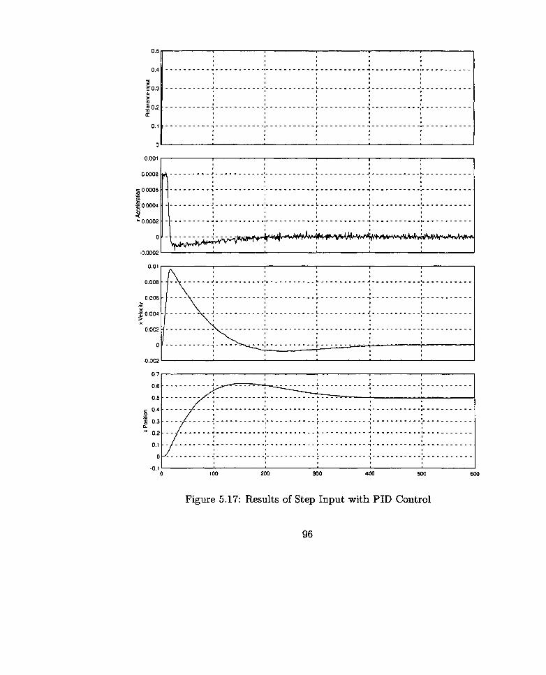
-0.1 1 I O 1 O0 200 300 400 500 600

Figure 5.17: Results of Step Input with PID Control

-0.0001 1 1

O 1 O0 200 300 400 500 600

dornain

Figure 5.18: Results of Disturbance Input

is stronger than al1 other influences. Thus, within its capacity, the DICE hub is holding station as required.

Figure 5.19: Control of Several Degrees of Fkeedorn

Chapter 6

Some Concluding Remarks

6.1 What Has Been Learned?

It can be concluded from the foregoing work that the preliminary design of a stationkeeping systern for a free-flyer in the middeck has been a successful one.

The major dist urbances to the bus have been identified and characterised in quite some detail. The resulting simulation of these disturbance forces has shown that the greatest of these disturbance forces is the air circulation, which exerts forces of up to 1 0 - ~ N and torques up to 10-4 Nm. However, the air circulation force is also the most fickle, as it depends on the number of air circulation sources and their locations with respect to the DICE bus. In the absence of air circulation forces, the remaining forces become the dominant ones, exerting combined forces of up to N and torques up to 10-~ Nm.

The actuation system designed to counter these forces makes use of the fact that NASA flight requirements demand the circulation of air in the interior of any middeck experiment that produces heat. The air which is pulled into the DICE bus for this purpose is then ejected tbrough a set of 3 nozzle clusters. Valves in those clusters control the amount of air ejected in each direction, thus producing a net thrust on the bus. Verification of this system by building a Bus Mock-up demonstrated that one nozzle could exert a maximum thrust of N. The Bus Mock-up also demonstrated that the efficiency of the system dropped significantly when interior elements were added to the bus, and, therefore, that the efficiency of the system could be improved with a little attention to the interior layout.

Since the disturbance forces are of low frequency and an order of magnitude lower than the force which can be exerted by the actuation system through one nozzle, this stationkeeping design can be judged a viable solution. However, further work must be done before this system can be accepted for Shuttle flight.

6.2 Recommendat ions for Furt her Work Fùrther work in the area of stationkeeping system design is mandatory

before such a system can be fully endorsed for the DICE project. In general, this involves extending the design work that has already been done and refining that work in response to both NASA flight requirements and the evolving design of the DICE bus as a whole. The following are particular items which will require future attention:

1. EVA Pressure

Al1 of the analysis in this document, both the disturbance simulation in Chapter 3 and the actuator design in Chapter 4, have been carried out assuming an atmospheric cabin pressure of 14.7 psi. However, during missions involving EVA, the cabin pressure is lowered to 10.2 psi. A sensitivity analysis should be made of the reaction of both the disturbance forces and the stationkeeping design to changes in cabin pressure.

2. ISS Construction

Many of the Shuttle flights in the foreseen future somehow involve the construction of or docking with International Space Station. The inclusion of ISS will impact on almost al1 of the disturbance forces included in the disturbance simulation of Chapter 3, in most cases increasing the magnitude of these forces. If the DICE experiments were carried out inside ISS, rather than the Space Shuttle middeck, the workspace and air circulation environment will also change. The impact of including ISS in the disturbance analysis should be exarnined.

3. Interna1 Air Flow

It was seen in Chapter 5 that large energy losses were incurred inside the DICE bus, and that there were some problems associated with the

air inlets and the interior circulation of air in the bus. Further thought should go iato the arrangement of interior bus elements and the ducting of air inside the bus, in order to resolve the problems identified in Chapter 5.

4. Bus Mock-up Extension

The Bus Mock-up has proven to be a very useful tool for design verification, and an extension of the work already done should be made. In particular, al1 nozzles of the Bus Mock-up should be equipped with valves and mot orized valve servos, and simult aneous measurernents of air flow frorn several nozzles should be made to judge the sensitivity of nozzles with respect to each other. The power drawn by the system should also be measured, as well as the pressure distribution within the bus volume to verify whether the bus is truly acting as a plenum. The problem of providing each 'thruster cluster' with pressure identical to the others is one that deserves immediate attention, and may change the direction of the present plenum design.

5. Momentum Dumping

The issue of momentum dumping has been ignored in this thesîs due to its ill-defined nature at this point in the project. Nevertheless, it is a requirement that the DICE stationkeeping system provide momentum dumping to the bus, and the impact of this requirement on the actuators should be exarnined in detail in the future

6 . Space Shuttle Safety

In addition to al1 its technical requirements, the stationkeeping system must also concur with NASA's safety requirements for middeck experiments. As those requirements are not yet known, an effort should be made to identify al1 such requirements and insure that the stationkeeping system is designed to meet them.

Bibliography

[l] Canadian Space Agency. http: //radarsat .space.gc .ca. Last revised: February 19, 1997.

[2] Robert C. Blanchard and Gregory M.Buck. Rarefied-flow aerodynamics and t hermosphere structure from Shuttle flight rneasurements. Journal of Spacecraft and Rockets, pages 18-24, January 1986.

[3] K.A. Carroll. Definition of in-orbit experiments on the dynamics and control of large flexible space structures: (DICE): Phase 1. Technical Report 29-41 1 / 15- 1, Dynacon Enterprises Limited, March 1995.

[4] Nicholas P. Cheremisinoff and Paul N. Cheremisinoff. Cornpressors and Fans. Process and Pollution Control Equipment. Prentice Hall, Inc., New Jersey, 1992.

[5] J .M. Crawfor d. D ynamics identification and control exper iment (DICE) Topics Report: Shuttle middeck environment disturbances. Technical report, University of Toronto Institute for Aerospace Studies, June 1995.

[6] Edward F. Crawley. MODE and Its Impact. Presentation Slides.

[7] Edward F. Crawley, Marthinus C. Van Schoor, and Edward B. Bokhour. The Middeck O-Gravity Dynamics Experiment: Summary report. NASA Contractor Report 4500, Massachusetts Institute of Technology, 1993.

[8] Edward F. Crawley, Principal Investigator. Middeck O-Gravity Dynam- ics Experiment (MODE-3). Technical report, Massachusetts Institute of Technology, March 19%.

[9] CRC Press, Ohio. CRC Handbook of Tables for Applied Engineering Science, 2nd ed. edition, 1973.

[IO] Environmental Science Services Administration, National Aeronautics and Space Administration, and United States Air Force. U.S. Standard Atmosphere Supplements, 1966, 1966.

[Il] B.J. Dunbar et al. The microgravity environment of the Space Shuttle Columbia middeck during STS-32. NASA TP-3140, NASA Scientific and Technical Information Program, 1991.

[12] Paul Fulford and Craig Thronton. Operational concepts document, 1995. Course Notes fiom Space Systems Design Course, University of Toronto.

[13] M.D. Griffin and J.R. fiench. Space Vehicle Design. AIAA Education Series. American Institute of Aeronautics and Astronautics, Inc., 1991.

[14] Guidance and Control. Spacecraft mass expulsion torques. Technical Re- port NASA SP-8034, National Aeronautics and Space Administration, 1969.

[15] Guidance and Control. Spacecraft radiation torques. Technical Report NASA SP-8027, National Aeronautics and Space Administration, 1969.

[16] Guidance and Control. Technical Report NASA SP-8000, National Aero- nautics and Space Administration, 1970.

[l?] Hans Harnacher. Spacecraft low-fiequency residual acceleration. Journal of Spacecraft and Rockets, 32(2), March 1995.

[18] Johanne Heald. Design of an air thruster system for the stationkeeping and attitude control of DICE and the engineering model. Univerisity of Toronto, April 1995. B.A.Sc. Thesis.

[19] Johanne Heald. Recirculation system hardware assessment. Report of Findings from Task 5, April 1996.

(201 P.C. Hughes. Research Proposa1 for DICE Project. Submitted to NSERC, 1994.

[21] P.C. Hughes. Course Notes: Spacecmft Dynamics Ei Contml - I. Univer- sity of Toronto Institute for Aerospace Studies, Spring 1995. AER506S.

1221 P[eter]. C. Hughes. Spacecmft Attitude Dynamics. John Wiley and Sons, Inc., 1986.

1231 J .R.Leigh. Applied Control Theory. IEE Control Engineering Series 18. Short Run Press Ltd., Exeter, England, 1982.

[24] Douglas G . MacMartin and David W. Miller. MIT Middeck Active Control Experiment (MACE): Non-collocated payload pointing control. Space Engineering Research Center, Dept. of Aeronautics and Astro- nautics, Massachusetts Institute of Technology, 1994.

[25] M. J . Malone. Aerospace laboratory experiments: First set, September 1996. AER 303F.

1261 J.E. Moore, J. Shepphard, J. Pizzacaroli, P. Lyman, and H.R. War- ren. Radarsat: The bus and solar array. Canadian Journal of Remote Sensing, l9(4), November 1993.

[27] NASA and Rockwell International Corporation. Shuttle/Payload Inter- face Definition Document for Middeck Payloads, rev. A edition, Novem- ber 1992. STS Interface Control Document.

[28] National Oceanic and Atrnospheric Administration, National Aeronau- tics and Space Administration, and United States Air Force. U.S. Stan- dard Atmosphere, 1976, 1976.

[29] Cuong Q. Nguyen. Johnson Space Center STS summary notes. NASA JSC Document, 1997.

1301 Phung Nguyen. DICE experiment plan. Technical Report DICE1, Uni- versity of Toronto Institute for Aerospace S tudies, December 1995.

131) C. Osborne. The Setection and Use of Fans. Design Council, British Standards Institution and Council of Engineering Institutions. Engi- neering Design Guides.

[32] Stephen Piggot. Flight mode1 AutoCAD drawings, December 1996.

[33] M.A. Plint and L. Boeswirth. Fluid Mechanics: A Labomtory Course. Charles Griffin and Company Ltd., 1978.

[34] Shasti Kant Shrivastava. Orbital perturbations and stationkeeping of communications satellites. Journal of Spacecraft and Rockets, 15(2), March 1978.

[35] U.S. Space and Rocket Center, Huntsville, AL. U.S. Space Academy Level II Tkaining Manual, 1990.

1361 James Wertz. Spacecmft Design. AIAA Inc., 1991.

Appendix A

Thesis Task List

Task 01 Review and confirm previous DICE disturbance work (primarily that in 151)

Task 02 Survey literature to compile the possible disturbances to DICE in the Space Shuttle Orbiter middeck

Task 03 Identify the DICE workspace in the middeck

Task 04 Propose a baseline stationkeeping system actuator design

Task 05 Create math model of DICE disturbance environment

Task 07 Construct a simulation of the DICE disturbance enivironment based on the math model

Task 08 Define the criteria for the evaluation of the DICE stationkeeping system

Task 09 Design and build a mockup of the flight version of the DICE bus, including interior elements and exit nozzles

Task 10 Evaluate the performance of the actuators in use on the IPM

Task 11 Characterise the airflow through the Bus Mock-up and evaluate the performance of the actuators

Task 12 Identify the essential actuator characteristics for simulation

Appendix B

Orbiter Characteristics

The inertia matrix for the Space Shuttle Orbiter used in this document is

Note that

Orbiter mass used in this document corresponds to that in [35], which is 68 500 kg.

The location of the Orbiter center of pressure was calculated using the counting squares method. In the Shuttle coordinate system, the center of pressure is located at (1 l92,O ,270) inches.

Appendix C

XMath/Systembuild Code for Disturbances

The following pages contain the S ystembuild blocks used to simulat e the disturbance environment on DICE. Also included are the XMath mathscript functions which support certain blocks in the simulation. In order to run the simulation, the variables in the set-parameters-msf function must be loaded into XMath. First, set the directory path to home/jhe/simulation/proto. Then type

set -paramet ers() ;

at the Command Line in XMath. This creates the partition 'dist' to keep al1 disturbance simulation variables together, and loads those variables into that partition. If it is desirable to change the values of those variables (Space Shut- tle orbital altitude, for example), it should be done in the set-parametersmsf file, and the above cornmand should be repeated.

Once the simulation variables have been loaded, change to the 'dist' partition. A unit vector of the same size as the time vector, t, must be created by ty ping

in order to run the simulation. This variable u must have the same number of columns as the block to be simulated has inputs. Finally, the simulation can be run with the command

where BlockNurne is the name of the block to be simulated in quotation marks (" Hub Dist urbances" , for example).

The code for each Mathscript function is given below.

C . l set -parameters.msf

#{ Title: set -parameters.msf Function: Set al1 initial variables Author: Johanne Heald Modified: 20/03/97 Purpose: To allow al1 parameters for the disturbance simulation to be set

before the test runs. Input: none Output: flag indicating success

)#

Function[flag] = set -parameters();

# Create partitions so variables correspond with Eric Choi's code if !exist (dice,{partition} ) ;

new partition dice; endIf; if !exist(disturb,{partition));

new partition dist; endIf; set path = " $SYSBLD/bin" ; # Set disturbance parameters

dist.simLength = 1*60; # Simultion duration (sec) diststepsize = 1; # Step size for simulation (sec) dist.t=[O:dist .stepsiae:dist.simLength]'; # time vector for simulation dist.a = 450; # Shuttle orbit altitude (km) dist.i = 0/360*2*3.14; # Shuttle orbit inclination (rad) dist.n = 0.0012 # Shuttle mean orbital rate (rad/s) dist.0 = 1; # Shuttle orbit type dist.DSur = 1; # Shuttle surface facing Earth dist.FSur = 4; # Shuttle surface facing dir. of travel

dist.PV = [0,0,0]; # Matrix defining shuttle orbit dist.D = 3.14; # Time of year in solar orbit (rad) dist.S =2000; # Time of closest orbit approach to # Sun (sec) dist.DA = [64.1*2,64.1*2.2;367*2.2,367*2.2;212.7'2.2,212.7*2.2]; dist.Diurna1 = [1.068,1.053,1.043,1.038,1.037,1.04,1.049,1.069,1.097,1.133,1~172, 1.208,1.238,1.258,1.266,1.263,1.251,1.232,1.209,1.184,1.159,1.133, 1.109,1.087]; # Vector definiag diurnal effect dist.CP = [1192,0,270]/(12*3.3); # Shuttle center of pressure (m) dist.CM = [1080,0,380]/(12*3.3); # Shuttle center of mass (m) dist.ShuttleMass = 68500; # Shuttle mass (kg) dist.DICEMass = 50/2.2; # DICE mass (kg) dist .ShuttleInertl = 1206677; dist .ShuttleInert2 = 9450050; dist .ShuttleInert3 = 9829679; # Shuttle inertia dist .Ml = dist .ShuttleInert3 - dist .ShuttleInertl; dist.1113 = dist.ShuttleInert1 - dist.ShuttleInert3; dist .I211 = dist .ShuttleInert2 - dist .ShuttleInertl; # Shuttle inertia factors for gradient dist .DICEInert 1 = 0.0477 dist.DICEInert2 = 0.00923 dist .DICEInert3 = 0.00923; # DICE inertia (kgm4) dist-Originx = 490/(12*3.3); # DICE origin in Shuttle (m) dist .Originy = 0; dist.Originz = 370/(12*3.3); dist.rl = dist.CM(1) - dist.Originx; dist .r2 = dist.CM (2) - dist.Originy; dist .r3 = dist.CM (3) - dist.Originz; dist xinit = (dist .CP(l)-dist .Originx); dist .yinit = (dist .CP(2)-dist.Originy); # initial offset of DICE from CP dist.FLockerx = 24/(12*3.3); # distance bwt DICE and Front lockers dist.ALockerx = 42/(12*3.3); # distance btw DICE and Aft Lockers (m) dist.Diameter = 0.05; # Middeck locker fan diameter (m) dist.vd = 2; # Middeck fan exit air velocity (m/s) dist.FlowTurbulence = 10; # Laminar = 10, Turbulent = 3.3 # Middeck locker fan positions (m) # (relative t o DICE origin) dist.Fly = 0;

dist .F lz = 121 (lS*3.3); dist.F2y = 9/(12*3.3); dist.F2z = 6/(12*3.3); dist.F3y = 9/(12*3.3); dist.F3z = 0; dist.F4y = 9/(12*3.3); dist .F4z = -6/(12*3.3); dist.F5y = 0; dist.F5z = 6/(12*3.3); dist.F6y = 0; dist.FGz = -6/(12*3.3); dist.F7y = -9/(12*3.3); dist.F7z = 6/(12*3.3); dist.FBy = -9/(12*3.3); dist.F8z = 0; dist.F9y = -9/(12*3.3); dist.F9z = -6/(12*3.3); dist .Aly = -18/(12*3.3); dist.Alz = 6/(12*3.3); dist.AZy = -18/(12*3.3); dist.A2z = 0; dist.A3y = -18/(12*3.3); dist.A3z = -6/(12*3.3); dist.A4y = -9/(12*3.3); dist.A4z = 6/(12*3.3); dist.A5y = -9/(12*3.3); dist.A5z = 0; dist .A6y = -9/(12*3.3); dist.A6z = -6/(12*3.3); dist.cabinden = 1.2 # Middeck cabin air density (kg/m3)

flag = 1; endFunction;

#{ Title: drag.msf Fùnction: Calculate some drag components Author: Johanne Heald Modified: 19/02/97 Purpose: To calculate the drag coefficient and area and unit vector of the

force direction in shuttle coordinates Input: shuttle orientation, CdA Matrix Output: Cd*Area*unit vector

)#

VecSize = size(angle1); for j = l:VecSize(l)

01 = angle1 (j); 02 = angle2(j); 03 = angle3(j); if ((abs(o2) < pi) & (abs(o3) < pi)) BF = 1; # BF = Back(=2)/Fkont(=l) else; BF = 2; endIF; if ((02 < 2*pi) & (02 > O) & (abs(o1) < pi)) TB = 2; # TB = Top(=l)/Bottom(=2) else; TB = 1; endIF; if ((03 < 2*pi) & (03 > O) & (abs(o1) < pi)) SS = 1; # SS = Side(Left=2)/Side(R=l) else; SS = 2; endIF; DragArea = COS(O~) * (cos(o2) *CdA(l ,BF) ) + sin(o3)*(sin(ol)*CdA(2,TB)+cos(ol)*CdA(3,SS)); phi = -02;

th = -01; psi = -03; Trans(l,l) = cos (psi) *cos(phi) - sin(psi) *sin(th) *sin(phi) ; Trans(l,2) = -sin(phi) *cos(th); nans( l ,3) = sin(psi)*cos(phi) + cos(psi) *sin(phi)*sin(th) ; Trans(2,l) = cos(psi)*sin(phi) + sin(psi)*cos(phi)*sin(th); Tkans(2,2) = cos (phi)*cos(th) ; Tkans(2,3) = sin(psi) *sin(phi) - cos(psi) *cos(phi) *&(th) ; Trans(3,l) = -sin(psi)*cos(th) ; Trans (3,P) = sin ( t h) ; Srans(3,3) = cos (psi) *cos (th); FV = Trans * [1,0,0]'; fx(j) = DragArea*FV(l); fy(j) = DragArea'FV(2); fz(j) = DragArea*FV(3);

endFor ; endhnct ion;

#{ Title: density.msf Function: Calculate the atmospheric density Author: Johanne Heald Modified: 13/02/97 Purpose: To calculate the density of the atmosphere at a partjcular time

in the Orbiter's orbit. Input: tirne, start time of orbit, altitude, diurnal effect vector Output: density )#

Function[density] = density (time,Tsun,a,DEffect )

T = 1 lO*log(lOO*(a-119))- 140; VecSize = size(time); for j= 1 :VecSize(l)

HTMid = round((l2 - ((Tsun-time(j))*24/(90*60))),up); if (HTMid < 0) HTMid = HTMid + 24; endIf; T = T*DEffect (HTMid); gradT = 110/(a-119); Beta = (9.8/0.28 + gradT)/T density(j) = (2.5e-08*exp(-Beta*(a-119)));

endFor; endhnc t ion;

#I Title: solar.msf Function: Calculate Shut tle Orbiter Orientation wrt Sun Author: Johanne Heald Modified: 25/02/97 Purpose: To calculate, a t any point in its orbit, the orientation of the

Space Shuttle Orbiter relative to the position of the Sun, and t o find the Absorption Coefficient*Area of the shuttle in that orientation.

Input : orbit time, shuttle orientation, orbit inclination, time of closest solar approach, altititude

Output: KA = absorption*area;

)#

hinction [xka] = solar(t,vl,v2,v3,i,TSun,a)

n = 2*pi/(90*60); umbra = (3.14 - acos(-6378/(6378 + a)))/6.28; VecSize = size(t); for j = l:VecSize(l) if (abs(t(j)-TSun) < ((6.28/n)*(0.25+umbra)) ) abs(t(j)-TSun)

> ((6.28/n)* (0.75-umbra))) # Shuttle not in Earth's umbra phi = -v2(j); t h = -vl(j); psi = -v3(j); v = [cos(vl(j));cos(v2(j));cos(v3(j))]; theta = (t(j) - TSun)*n; EarthInc = 23.5*2*pi/360; #Earth's inclination to the Sun if theta i pi I = i - EarthInc; else 1 = EarthInc - i; endIf; Csuninc = [cos(I) ,-sin(1) ,O;sin(I) ,cos(I) ,0;0,0,1] ; #C3 rotation Cincorb = [cos(theta) ,O,sin(theta);O, 1,O;- sin(theta) ,O,cos(theta)];

#c2 rotation Sun = Csuninc*Cincorb*v; SunSize = sqrt(sun(l)9 + ~ u n ( 2 ) 2 + ~un(8)q); Sun = Sun/SunSize; 01 = acos(Sun(1)); 02 = acos(Sun(2)); 03 = acos(Sun(3)); if ((abs(o2) < pi) & (abs(o3) i pi)) KA1 = 1.3*64.1; else; KA1 = 1.58*64.1; endIf; if ((02 < 2*pi) & (02 > O) & (abs(o1) < pi)) KA2 = 1.4*367; else; KA2 = 1.02*367; endIf; KA3 = 1.4*212.7; SolArea = abs(cos(o3) *cos(ol)*KA2) +abs(sin(o3) *cos(o2)*KA 1) + abs(sin(o2) *sin(ol ) *KA3) ; forcevec = SolArea* [O;O;- ï ] ; w = inv(Cincorb) *inv(Csuninc)* forcevec; Trans(1,l) = cos(psi) *cos(phi) - sin(psi) *sin(th) *sin(phi) ; Trans(1,l) = -sin(phi)*cos(th); nans ( l ,3 ) = sin(psi) *cos(phi) + cos(psi)*sin(phi) *sin(th); nans(2 , l ) = cos(psi) *sin(phi) + sin(psi)*cos(phi) *sin@) ; Trans(2,2) = cos(phi) *cos(th) ; nans(2,3) = sin(psi) *sin(phi) - cos(psi) *cos(phi)*sin(th); nans(3 , l ) = -sin(psi) *cos(th); ?tans(3,2) = sin(th); Trans (3,3) = cos(psi) *cos(th) ; w = T r a n s * ~ ; xka(jll) = w(1); *W,2) = ~ ( 2 ) ; *(j13) = ~ ( 3 ) ;

else; # Shuttle in Earth's umbra xka(j,l) = O;

xka(j,2) = O; xka(j,3) = O;

endIf; endFor ; endFunct ion;

C.5 orient .msf

#{ Title: orient .msf Function: Calculate Shut tle Orbiter Orientation Aut hor : Johanne Heald Modified: 15/02/97 Purpose: To calculate, at any point in its orbit, the orientation of the Space Shuttle Orbiter relative to the standard 3-axis orbit coordinat es. Standard 3-axis cooridinates: x = direction of travel z = line connected to center of Earth y = 3rd axis in RH set Input: orbit time, orbit type, Output: v(l:3) = roll (about x), pitcb (about y), yaw (about a )

l# Function [vl ,v2,v3] = orient ( t ,u,Otype,downwardSur,forwardS~to);

if Otype == 1; if forwardsur == 1; v2 = o*u; v3 = o*u; if downwardsur == 4; v l = o*u; else; v l = 3.14*u; endIf; elseif forwardsur == 3; v2 = o*u; v3 = 3.14*u; if downwardsur == 4; v l = o*u; else; v l = 3.14*u; endIf; elseif forwardsur == 2; v l = o*u;

v2 = 1.57*u; if downwardsur == 1; v3 = o*u; else; v3 = 3.14*u; endIf; elseif forwardsur == 4; vl = O*u; v2 = -1.57*u; if downwardsur == 3; v3 = o*u;; else; v3 = 3.14*u; endIf; elseif forwardsur == 5; v l = o*u; v3 = 1.57*u; if downwardsur == 4; v2 = o*u; elseif downwardsur == 3; v2 = -1.57*u; elseif downwardsur == 2; v2 = 3.14*u; else; v2 = 1.57*u; endIf; elseif forwardsur == 6; v l = o*u; v3 = -1.57*u; if downwardsur == 4; v2 = O*u; elseif downwardsur == 3; v2 = - 1 . 5 7 * ~ ; elseif downwardsur == 2; v2 = 3.14"~; else; v2 = 1.57*u; endIf;

endIf; elseif Otype == 2;

v l = pointto(1,l) + t/5400*0; v2 = pointto(1,Z) + t/5400*0; v3 = pointto(l,3) + t/5400*6.28;

elseif Otype == 3; n = round(t/ôO) + 1; v l = pointto(n,l); v2 = pointto(n,2); v3 = pointto(n,3);

endIf; endhnction;

Title: torquecp.msf Function: Calculate the torque about the mass center Author: Johanne Weald Modified: 18/02/97 Purpose: To calculate the torque about the Space Shuttle mass center produced by a force acting though the center of pressure. Input: cp location, mc location, force vector in force direction (shuttle coordinat es) Output: 3 force components on shuttle mass center, 3 torque components on shuttle mass center

)#

Funct ion [tor] = torquecp (xforce, yforce,zforce,cp,cm)

VecSize = size(xforce) ; for j=l:VecSize(l)

forcemag = sqrt (xforce(j) + yforce(j)î + zforce(j)î); if forcemag <> O ik = xforce(j) /forcemag; fy = yforce(j)/forcemag; f i = zforce(j)/forcemag; else; fx = 0; fy = O; f i = O; endIf; V = (cp - cm); D = V - (V(l)*bc + V(Î)*fy + V(3)*tz)*[£x,fy,fz]; T = [(D(2)*zforce(j)-D(3)*yforce(j)),(D(3)*xforce(j)- D(l)*zforce(j)), (D(l)*yforce(j)-D(2)*xforce(j))]; tor(j,l) = T(1); tor(j,2) = T(2); tor(j,3) = T(3);

endFor ; endFunction;

#{ Title: @rame-msf Fùnction: Change force reference frames Author: Johanne Heald Modified: 29/01/97 Purpose: To calculate the forces on DICE which result £rom a force on the Shuttle m a s center. Input: force on shuttle, DICE orientation, shuttle mass, DICE mass Output: forces on DICE

1#

acc = [Fl,F2,F3]'/massS; Force = massD*acc; phi = Ox; th = Oy; psi = Oz; Trans(1,l) = cos(psi)*cos(phi) - sin(psi)*~in(th)*sin(~hi); Trans(1,S) = -sin(phi) *cos(th); Trans(l,3) = sin(psi) *cos(phi) + cos(psi)*sin(phi) *çin(th); Trans(2,l) = cos(psi) *sin(phi) + sin(psi) *cos(phi) *sin(th) ; Trans(2,S) = cos(phi) *cos(th); Trans(2,3) = sin (psi) *sin(phi) - cos(psi) *cos(phi) *sin(t h) ; Trans(3,l) = -sin(psi) *cos(t h); Trans(3,2) = sin(th); 'llans(3,3) = cos(psi)*cos(th) ; FV = Trans * Force; fx = FV(1); fy = FV(2); fi = FV(3); endhnction;

#( Title: frame.msf Function: Change torque reference frames Author: Johanne Heald Modified: 29/01/97 Purpose: To calculate the forces and torques on DICE which result Fom a torque on the Shuttle mass center. Input: torque on shuttle, DICE position, DICE orientation, origin posi-

tion shuttle inertia, DICE inertia Output: forces on DICE, torques on DICE

)#

tx = - Tl/SIne(l) * DIne(1); ty = - T2/SIne(2) * DIne(2); t z = - T3/SIoe(3) * DIne(3); wdot (1) = -Tl/SIne(l); wdot(2) = -T2/SIne(2); wdot (3) = -T3/SIne(3); Elapsed = time - prevAcc(1); w(1) = (wdot(1) - prevAcc(2))/Elapsed; w(2) = (wdot (2) - prevAcc(3))/Elapsed; w (3) = (wdot (3) - prevAcc(4))/Elapsed; D = [(Dx+OPos(l)),(Dy+OPos(2)),(Dz+OPos(3))]; wcross = [-w(3) ,w(l) ,O; w(2) ,O,-w(1); 0,-w(2),w(3)]; wdotcross = [-wdot(3) ,wdot(l) ,O; wdot (2),0,-wdot(1); O,- wdot (2),wdot (3)]; rnot = [vx,vy,vz]' - wcross*D'; acc = S*wcross*rnot + wcross*(wcross*D') + wdotcross*D7; Force = massD*acc'; prevAcc(1) = time; prevAcc(2) = wdot (1); prevAcc(3) = wdot(2); prevAcc(4) = wdot (3) ;

phi = Ox; th = Oy; psi = Oz; Trans (1,l) = cos(psi) *cos(phi) - sin(psi) *~in(th)*sin(~hi); Trans (l,2) = -sin(phi) *cos(t h) ; Trans(l,3) = sin(psi)*cos(phi) + cos(psi)*sin(phi)*sin(th); Tkans (2, l ) = cos(psi) *sin(phi) + sin(psi) *~os(~hi)*sin(th); nans(2,2) = cos(phi) *cos(th); Tram (2,3) = sin(psi)*sin(phi) - cos(psi)*cos(phi)*sin(th); Trans (3,l) = -sin(psi) *cos(th); Trans(3,2) = sin(th); Trans(3,3) = cos(psi)*cos(th); FV = Trans * Force'; fx = FV(1); fy = FV(2); f i = FV(3);

endhnction;

C.9 Systembuild Blocks The first set of Systembuild blocks consists of those which make up the simulation precalczl1ated.s ysbld. In this case, no inputs are required, other than the unity vector and the time vector. The output forces are independent of the position of DICE in the Orbiter middeck. Therefore, these disturbances can be 'precalculated' ahead of time, so long as the Space Shuttle orbital characteristics are known.

The second set of Systembuild blocks make up the simulation wntime.sysbld. In this case, the forces are dependent upon the position of DICE in the Space Shuttle middeck. Hence, this simulation must be run in parallel with any control or system identification experiments which might alter the location of DICE. In this case, the output forces of this simulation become the disturbance inputs in the much larger control system.

C.9.1 Hub Disturbances

Inputs:

1. Vector of ones (same size as t )

Outputs:

1. Force on DICE in x direction (SVS frame of reference)

2. Force on DICE in y direction (SVS frame of reference)

3. Force on DICE in z direction (SVS frame of reference)

4. Torque on DICE about x axis (SVS frame of reference)

5. Torque on DICE about y axis (SVS fiame of reference)

6. Torque on DICE about z axis (SVS frame of reference)

Figure C. 1: Precalculated Hub Disturbances

132

C.9.2 Atmospheric Drag

Inputs:


Outputs:

1. Force on Space Shuttle in x direction (Shuttle frame of reference)

2. Force on Space Shuttle in y direction (Shuttle frame of reference)

3. Force on Space Shuttle in z direction (Shuttle frame of reference)

4. Torque on Space Shuttle about x axis (Shuttle fiame of reference)

5. Torque on Space Shuttle about y axis (Shuttle frarne of reference)

6 . Torque on Space Shuttle about z axis (Shuttle frame of reference)

C .9.3 Solar Radiation

Inputs:

1. Vector of ones (same size as t)

Outputs:

1. Force on Space Shuttle in x direction (Shuttle fiame of reference)

2. Force on Space Shuttle in y direction (Shuttle fiame of reference)

3. Force on Space Shuttle in z direction (Shuttle frame of reference)

4. Torque on Space Shuttle about x axis (Shuttle frame of reference)

5. Torque on Space Shuttle about y axis (Shuttle frame of reference)

6. Torque on Space Shuttle about z axis (Shuttle frame of reference)

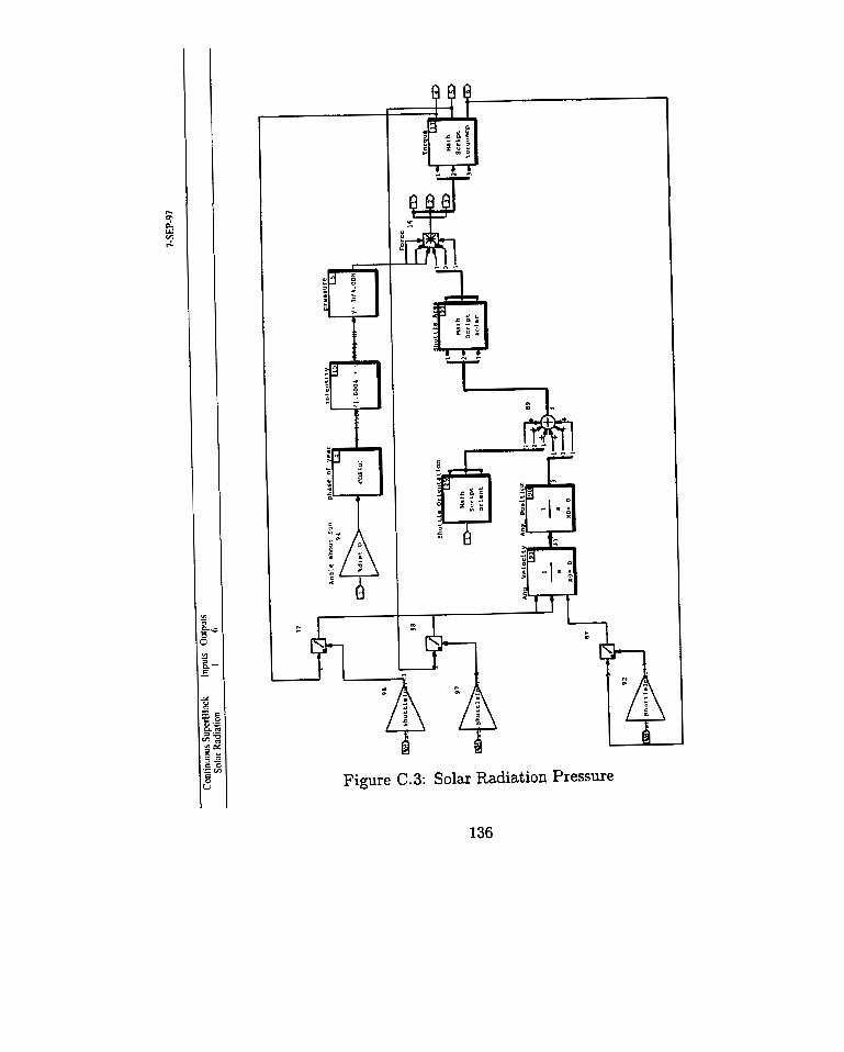
Figure C.3: Solar Radiation Pressure

136

C.9.4 Gravity Gradient Torque

Inputs:


Outputs:

1. Torque on Space Shuttle about x axis (Shuttle frame of reference)

2. Torque on Space Shuttle about y axis (Shuttle fiame of reference)

3. Torque on Space Shuttle about z axis (Shuttle frame of reference)

II-

Figure C.4: Gravity Gradient Torque

C.9.5 Total Run-tirne Disturbances

Inputs:


2. Acceleration in x direction (in DICE fiame of reference)

3. Acceleration in y direction (in DICE frame of reference)

4. Acceleration in z direction (in DICE fiame of reference)

5. Angle about x axis (in DICE frame of reference)

6. Angle about y axis (in DICE frame of reference)

7. Angle about z axis (in DICE frame of reference)

Ouputs:

1. Force on DICE along x axis (DICE frame of reference)

2. Force on DICE along y axis (DICE frame of reference)

3. Force on DICE along z axis (DICE frame of reference)

4. Torque on DICE about x axis (DICE frame of reference)

5. Torque on DICE about y axis (DICE frame of reference)

6. Torque on DICE about z axis (DICE frame of reference)

Figure C.5: Runtime Hub Disturbances

140

C.9.6 Locker Fans

Inputs:


2. Position in x direction (in DICE frame of reference)

3. Position in y direction (in DICE kame of reference)

4. Position in z direction (in DICE frarne of reference)

5. Angle about x axis (in DICE fiame of reference)

6. Angle about y axis (in DICE frame of reference)

7. Angle about z axis (in DICE frarne of reference)

Outputs:




4. Torque on DICE about x axis (DICE frame of reference)

5. Torque on DICE about y axis (DICE frame of reference)

6. Torque on DICE about z axis (DICE frame of reference)

Continuous SupcrBlock lnpuls Ouiputs Locker Fans 7 6

-l

Fan Force Torgue [IF----

1 - L7 -.

Conclnuoum ' -

I I I

2 - ~ontinuoui -

I

Fan Force Tor ue (IS u, A

A

Force from a Fan

Inputs:


2. Fan jet velocity along symmetry axis (SVS îrame of reference)

3. Fan y location on middeck waJ (Shuttle frarne of reference)

4. Fan z location on middeck wall (Shuttle frame of reference)

5. DICE x location in middeck (SVS frame of reference)

6. DICE y location in middeck (SVS frame of reference)

Outputs:

1. Fan force along z axis (SVS frame of reference)

2. Fan torque about x axis (SVS frame of reference)

3. Fan torque about y axis (SVS frame of reference)

Cornparison Block: Y1 = U > O and U < 0.1; then Gain = 0.08 Y2 = U > 0.1 and U < 0.25; then Gain = 0.2 Y3 = U > 0.25 and U < 0.4; then Gain = 0.31 Y4 = U > 0.4 and U < 0.5; then Gain = 0.38 Y5 = U > 0.5 and U < 0.75; then Gain = 0.55 Y6 = U > 0.75 and U < 1; then Gain = 0.68 Y7 = U > 1 and U < 1.5; then Gain = 0.87 Y8 = U > 1.5; then Gain = 1

Figure C. 7: Middeck Fan Formulation

144

Standard Deviation

Inputs:


2. Position in z direction (in SVS frame of reference)

Outputs:

1. Velocity of air jet from fore middeck lockers

2. Velocity of air jet from aft middeck lockers

Figure C.8: Air Jet as a Standard Deviation

C.9.7 Orbital Offset Forces

Inputs:


2. Acceleration in x direction (in DICE fiame of reference)

3. Acceleration in y direction (in DICE frame of reference)

4. Acceleration in z direction (in DICE frame of reference)

5. Angle about x axis (in DICE £rame of reference)

6 . Angle about y axis (in DICE frame of reference)

7. Angle about z axis (in DICE fiame of reference)

Outputs:




Figure C.9: Orbital Offset Forces

148

Appendix D

Empirical Data from Air Flow Tests

The following is data taken during the air characterisation trials described in Chapter 5. Note that negative values do not indicate a negative pressure relative to atmospheric; rather, they indicate a pressure negative t o that at which the zero was set on the manometer. Measurernents should be corn- paired to the manometer levels (initial and final) which define the 'zero point' for that particular trial.

D.1 IPM Trials

(from nozzle bottom)

1 2 3 4 5 6 7 8 9

10 11 12 13 14 15 16 17 18

Final Man. Level Table D.1: Manometer 1 Thruster

(fiorn nozzle bottom) Initial Man. Leuel

Vertical Position 0.7 c m

Table D.2: Manometer Thruster

2.1 cm

J-

--

-- 1

.eadings (mm) for Left S

(frorn nozzle bottom) Initial Man. Level

1 2 3 4 5 6 7 8 9

10 11 12 13 14 15 16 17 18 19 20 21 22 23 24 25 26 27

Fznal Man. Level

4.6 cm 1

-L Table D.3: Manometer Readings Thruster

3.0 cm Vertical Position 0.8 cm 2.3 cm

Initial Man. Level Valve Position i

l

Table D.4: Manometer Ei adings (mm) for Di 3.0

erent Valve Positions, Left Thruster

D.2 BMU Trials

D.2.1 Empty Bus

Vertical Position (from nozzle bottom)

Initial Man. Level 1 2 3 4 5 6 7 8 9

10 11 12 13 14 15 16 17 18 19 20 21 22 23 24

Final Man. Level I & Table D.5: ~ a & n e t e r Readings (mm) for Le Thruster

Vertical Position (from nozzle bottom)

Initial Man. Level

I I I I

Table D.6: Manometer Readings (mm) for Right Thruster

Nozzle firnber 1 2 3 4 5 6 7 8 9 10 11 12

Force (9) f 0.1 g 0.9 1.4 1.1 0.4 2.0 2.1 0.9 1.1 1.8 1.8 0.6 1.0

Table D.7: Force Readings for Al1 Nozzles

D.2.2 Interior Elernents Installed in Bus

Valve Position Initial Man. Level

- Final Man. Level L I

Table D.8: Manometer Read Valve Positions, Left Thruster

I

ngs (mm) for Different

L I

Table D.9: Force Readings for Al1 Nozz:

1 Nozzle Nvrnber

Position (cm) 0.0 O .5 1 .O 1.5 2 .O 2.5 3.0 3.5 4.0 4.5 5 .O

Force (g} f 0.1 g 0.9

Force (g) * 0.1 g 1.9

11

1.8 1.4 0.9 0.9 O.? 0.3 0.2

0.04 0.0 0.0

Note: Frequency of 'jitter' too high for empirical measurement with this equipmenl

Time (s) O

1

Force (g) f 0.1 g

Table D. l l : Force Time Variations

Appendix E

XMat h/Systembuild Code for Actuators

The following pages contain the Systembuild blocks used to simulate the actuators and controllers in the stationkeeping system. Also included is the XMath mathscript function which must be added to the set-parameters.msf function. This will create the partition 'air' to keep al1 actuator simulation variables together, and loads those variables into that partition.

As with the disturbance simulations, unit vectors, and possibly zero vectors of the same size as the time vector, t , must be created to make up the input u. The same simulation command is carried out, although in this case, the BlockName is one of the Superblocks contained in the SystemBuild file airthrusters.~ ysbld.

E. 1 Additions to set -parameters.msf

#{ Title: pararneters.msf Fùnction: Set al1 initial variables Author: Johanne Heald Modified: 22/04/97 Purpose: To allow al1 parameters for the thruster simulation to be set

before the test runs. Input: none Output: flag indicating success

Funct ion [flag] = parameters();

# Create partitions so variables correspond with Eric Choi's code if !exist (dice,{partition});

new partition dice; endIf; if !exist (air,{partition});

new partition air; ni endIf; ni set path = "$SYSBLD/bin" ;

ni # Set air thruster parameters air.t = [1:1:60]'; # calibration position # for motors (rad) air.calibrate1 = 0; air.calibrate2 = 0; air.calibrate3 = 0; air.calibrate4 = 0; air.calibrate5 = 0; air.calibrate6 = 0; # conversion of voltage to # speed (assumed linear) air.motorspeed = 1.05; # (12 V = 120 rpm)

flag = 1; endFunction;

E.2 Systembuild Blocks This set of Systembuild blocks consists of those which make up the simulation airthruster. sysbld. Included are the model of an individual air thruster, the model of the stationkeeping system which includes 6 air thrusters, and two PID controller superblocks: one which controls one degree of fieedom (DOF), which is x in the case shown, and the other wéich controls al1 six channels of the stationkeeping system.

E.2.1 Air Thruster

Inputs:

1. Voltage to the motor (Volts)

2. Calibration factor for the valve (offset from zero)

Outputs:

1. Net force exerted by the thruster (Newtons)

Figure E. 1: Individual Thruster Mode1

E.2.2 Stationkeeping System

Inputs:


2. Input for DICE force in x direction (DICE frame of reference)

3. Input for DICE force in y direction (DICE frame of reference)

4. Input for DICE force in z direction (DICE frame of reference)

5. Input for DICE torque about x axis (DICE frame of reference)

6. Input for DICE torque about y axis (DICE frame of reference)

7. Input for DICE torque about z axis (DICE frame of reference)

Outputs:

1. Net force exerted by DICE in the x direction (DICE frame of reference)

2. Net force exerted by DICE in the y direction (DICE fiame of reference)

3. Net force exerted by DICE in the z direction (DICE fiame of reference)

4. Net torque exerted by DICE about the x axis (DICE frame of reference)

5. Net torque exerted by DICE in the y axis (DICE frame of reference)

6. Net torque exerted by DICE in the z axis (DICE frame of reference)

Figure E. 2: Stationkeeping System Mode1

E.2.3 Controller in One DOF

Inputs:


2. Vector of zeros (same size as t)

3. Disturbance acceleration for DICE hub (DICE fiame of reference)

Outputs:

1. Reference input position of DICE hub (DICE frame of reference)

2. Net acceleration of DICE hub (DICE frame of reference)

3. Net velocity of DICE hub (DICE frame of reference)

4. Net displacement of DICE hub (DICE frame of reference)

Figure E.3: Controller for One Degree of Freedom

168

E.2.4 Six Channel Controller

Inputs:


2. Disturbance force for DICE hub in x direction (DICE frame of reference)

3, Disturbance force for DICE hub in y direction (DICE frame of reference)

4. Disturbance force for DICE hub in z direction (DICE frame of reference)

5. Disturbance force for DICE hub about x axis (DICE frarne of reference)

6. Disturbance force for DICE hub about y axis (DICE frame of reference)

7. Disturbance force for DICE hub about z axis (DICE frame of reference)

8. Reference input position of DICE hub (DICE frame of reference)

Outputs:

1. Net displacement of DICE hub in x direction (DICE frame of reference)

2. Net displacement of DICE hub in y direction (DICE frame of reference)

3. Net displacement of DICE hub in z direction (DICE frame of reference)

4. Net displacement of DICE hub about x axis (DICE fiame of reference)

5. Net displacement of DICE hub about y axis (DICE frame of reference)

6. Net displacement of DICE hub about z axis (DICE frame of reference)

7. Sample error signal on channel 2

Figure E.4: hill Controller

170

APPLIED - IMAGE. Inc = 1653 East Main Street - - -. - - Rochester, NY 14609 USA -- -- - - Phone: 71 61482-0300 -- -- - - Fax: 71 61288-5989

Q 1993, Applied Image. Inc.. All Righls Reserved

Documents

S tationkeeping - University of Toronto T-Spacetspace.library.utoronto.ca/bitstream/1807/11782/1/mq29367.pdf · Abstract The Space Shuttle middeck is an unlikeIy place to hd a fiee-