www.drfrostmaths.com 1

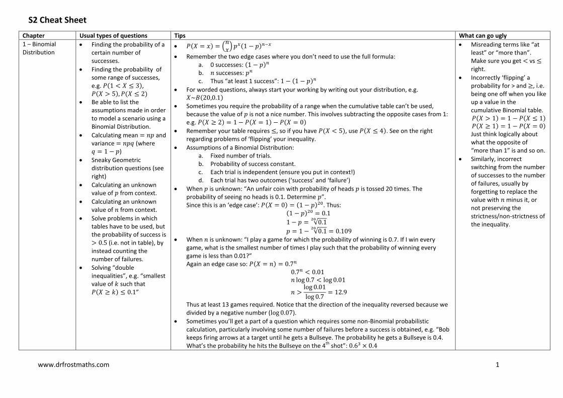
S2 Cheat Sheet

Chapter Usual types of questions Tips What can go ugly

1 – Binomial Distribution

Finding the probability of a certain number of successes.

Finding the probability of some range of successes, e.g. ( ), ( ) ( )

Be able to list the assumptions made in order to model a scenario using a Binomial Distribution.

Calculating mean and variance (where )

Sneaky Geometric distribution questions (see right)

Calculating an unknown value of from context.

Calculating an unknown value of from context.

Solve problems in which tables have to be used, but the probability of success is (i.e. not in table), by instead counting the number of failures.

Solving “double inequalities”, e.g. “smallest value of such that ( ) ”

( ) ( ) ( )

Remember the two edge cases where you don’t need to use the full formula: a. 0 successes: ( ) b. successes: c. Thus “at least 1 success”: ( )

For worded questions, always start your working by writing out your distribution, e.g. ( )

Sometimes you require the probability of a range when the cumulative table can’t be used, because the value of is not a nice number. This involves subtracting the opposite cases from 1: e.g. ( ) ( ) ( )

Remember your table requires , so if you have ( ), use ( ). See on the right regarding problems of ‘flipping’ your inequality.

Assumptions of a Binomial Distribution: a. Fixed number of trials. b. Probability of success constant. c. Each trial is independent (ensure you put in context!) d. Each trial has two outcomes (‘success’ and ‘failure’)

When is unknown: “An unfair coin with probability of heads is tossed 20 times. The probability of seeing no heads is 0.1. Determine ”. Since this is an ‘edge case’: ( ) ( ) . Thus:

( )

√

√

When is unknown: “I play a game for which the probability of winning is 0.7. If I win every game, what is the smallest number of times I play such that the probability of winning every game is less than 0.01?” Again an edge case so: ( )

Thus at least 13 games required. Notice that the direction of the inequality reversed because we divided by a negative number ( ).

Sometimes you’ll get a part of a question which requires some non-Binomial probabilistic calculation, particularly involving some number of failures before a success is obtained, e.g. “Bob keeps firing arrows at a target until he gets a Bullseye. The probability he gets a Bullseye is 0.4. What’s the probability he hits the Bullseye on the 4

th shot”:

Misreading terms like “at least” or “more than”. Make sure you get vs right.

Incorrectly ‘flipping’ a probability for > and , i.e. being one off when you like up a value in the cumulative Binomial table. ( ) ( ) ( ) ( ) Just think logically about what the opposite of “more than 1” is and so on.

Similarly, incorrect switching from the number of successes to the number of failures, usually by forgetting to replace the value with minus it, or not preserving the strictness/non-strictness of the inequality.

www.drfrostmaths.com 2

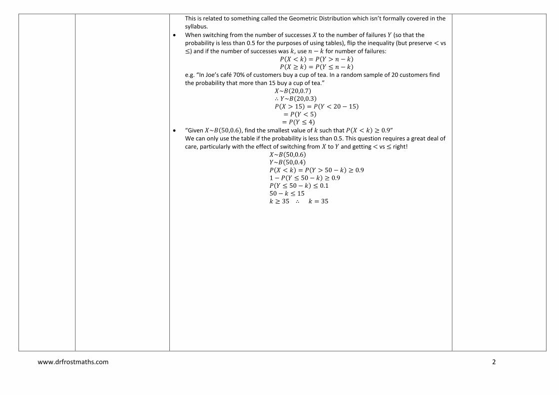
This is related to something called the Geometric Distribution which isn’t formally covered in the syllabus.

When switching from the number of successes to the number of failures (so that the probability is less than 0.5 for the purposes of using tables), flip the inequality (but preserve vs ) and if the number of successes was , use for number of failures:

( ) ( ) ( ) ( )

e.g. “In Joe’s café 70% of customers buy a cup of tea. In a random sample of 20 customers find the probability that more than 15 buy a cup of tea.”

( ) ( ) ( ) ( ) ( ) ( )

“Given ( ), find the smallest value of such that ( ) ” We can only use the table if the probability is less than 0.5. This question requires a great deal of care, particularly with the effect of switching from to and getting vs right!

( ) ( ) ( ) ( ) ( ) ( )

www.drfrostmaths.com 3

2 – Poisson Distribution

Be able to state the conditions under which a Poisson distribution may be used.

As with the Binomial Distribution, find the probability of a particular number of events happening within a given time frame, or within some range using tables.

State the mean and variance of a Poisson distribution.

Be able to scale a Poisson distribution to a different time period.

Feed the probability obtained from a Poisson distribution into a Binomial Distribution, and make subsequent calculations.

Approximate a Binomial Distribution using a Poisson Distributions, and be able to state the conditions under which we can do so.

Again, forming and solving ‘double inequalities’: e.g. “smallest value of such that ( ) ”

( )

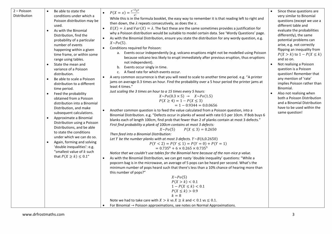
While this is in the formula booklet, the easy way to remember it is that reading left to right and then down, the repeats consecutively, as does the .

( ) and ( ) . The fact these are the same sometimes provides a justification for why a Poisson distribution would be suitable to model certain data. See ‘Wordy Questions’ page.

As with the Binomial Distribution, ensure you state the distribution for any wordy question, e.g. ( ).

Conditions required for Poisson: a. Events occur independently (e.g. volcano eruptions might not be modelled using Poisson

because volcano less likely to erupt immediately after previous eruption, thus eruptions not independent).

b. Events occur singly in time. c. A fixed rate for which events occur.

A very common occurrence is that you will need to scale to another time period. e.g. “A printer jams on average 0.3 times an hour. Find the probability over a 5 hour period the printer jams at least 4 times.” Just scaling the 3 times an hour to a 15 times every 5 hours:

( ) ( ) ( ) ( )

Another common question is to feed the value calculated from a Poisson question, into a Binomial Distribution. e.g. “Defects occur in planks of wood with rate 0.5 per 10cm. If Bob buys 6 blanks each of length 100cm, find prob that fewer than 2 of planks contain at most 3 defects.” First find probability a plank of 100cm contains at most 3 defects:

( ) ( ) Then feed into a Binomial Distribution: Let be the number planks with at most 3 defects. ( )

( ) ( ) ( ) ( )

Notice that we couldn’t use tables for the Binomial here because of the non-nice p value.

As with the Binomial Distribution, we can get nasty ‘double inequality’ questions: “While a popcorn bag is in the microwave, an average of 5 pops can be heard per second. What’s the minimum number of pops heard such that there’s less than a 10% chance of hearing more than this number of pops?”

( ) ( ) ( ) ( )

Note we had to take care with vs and vs .

For Binomial Poisson approximations, see notes on Normal Approximations.

Since these questions are very similar to Binomial questions (except we use a different table and evaluate the probabilities differently), the same potential problems can arise, e.g. not correctly flipping an inequality from ( ) to ( ) and so on.

Not realising a Poisson question is a Poisson question! Remember that any mention of ‘rate’ implies Poisson rather than Binomial.

Also not realising when both a Poisson Distribution and a Binomial Distribution have to be used within the same question!

www.drfrostmaths.com 4

3 – Continuous Random Variables

Find the probability of some range of values given a probability density function or cumulative distribution function. e.g. ( ) ( )

Appreciate that ( ) if is a continuous random variable.

State the probability density function given a graph.

Comment on the skew of a distribution.

Calculate ( ) ( ), the median/quartiles and the mode of a probability density function.

Convert from ( ) to ( ) and vice versa, potentially involving multiple ranges.

Be able to calculate ( ) (surprisingly common!)

Be able to calculate the median and quartiles.

Be able to calculate the mode, either by finding the turning point, or by inspection of the graph.

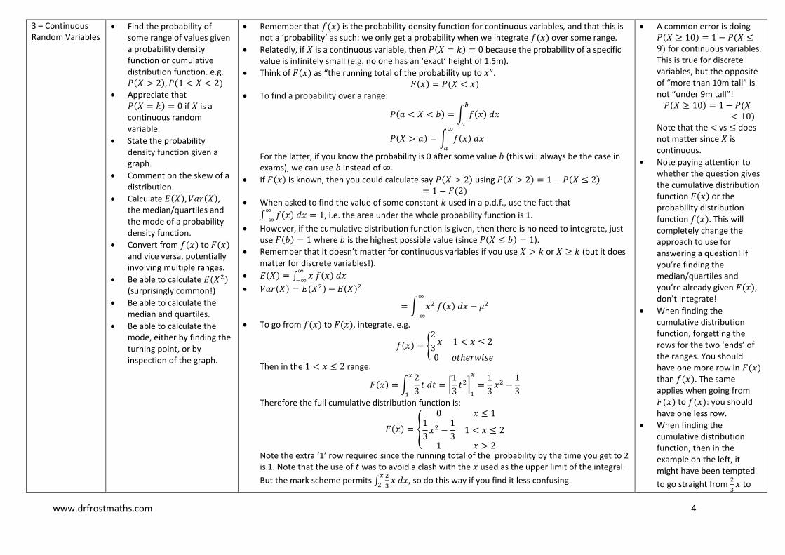
Remember that ( ) is the probability density function for continuous variables, and that this is not a ‘probability’ as such: we only get a probability when we integrate ( ) over some range.

Relatedly, if is a continuous variable, then ( ) because the probability of a specific value is infinitely small (e.g. no one has an ‘exact’ height of 1.5m).

Think of ( ) as “the running total of the probability up to ”. ( ) ( )

To find a probability over a range:

( ) ∫ ( )

( ) ∫ ( )

For the latter, if you know the probability is 0 after some value (this will always be the case in exams), we can use instead of .

If ( ) is known, then you could calculate say ( ) using ( ) ( ) ( )

When asked to find the value of some constant used in a p.d.f., use the fact that

∫ ( )

, i.e. the area under the whole probability function is 1.

However, if the cumulative distribution function is given, then there is no need to integrate, just use ( ) where is the highest possible value (since ( ) ).

Remember that it doesn’t matter for continuous variables if you use or (but it does matter for discrete variables!).

( ) ∫ ( )

( ) ( ) ( )

∫ ( )

To go from ( ) to ( ), integrate. e.g.

( ) {

Then in the range:

( ) ∫

[

]

Therefore the full cumulative distribution function is:

( ) {

Note the extra ‘1’ row required since the running total of the probability by the time you get to 2 is 1. Note that the use of was to avoid a clash with the used as the upper limit of the integral.

But the mark scheme permits ∫

, so do this way if you find it less confusing.

A common error is doing ( ) ( ) for continuous variables. This is true for discrete variables, but the opposite of “more than 10m tall” is not “under 9m tall”! ( ) (

) Note that the vs does not matter since is continuous.

Note paying attention to whether the question gives the cumulative distribution function ( ) or the probability distribution function ( ). This will completely change the approach to use for answering a question! If you’re finding the median/quartiles and you’re already given ( ), don’t integrate!

When finding the cumulative distribution function, forgetting the rows for the two ‘ends’ of the ranges. You should have one more row in ( ) than ( ). The same applies when going from ( ) to ( ): you should have one less row.

When finding the cumulative distribution function, then in the example on the left, it might have been tempted

to go straight from

to

www.drfrostmaths.com 5

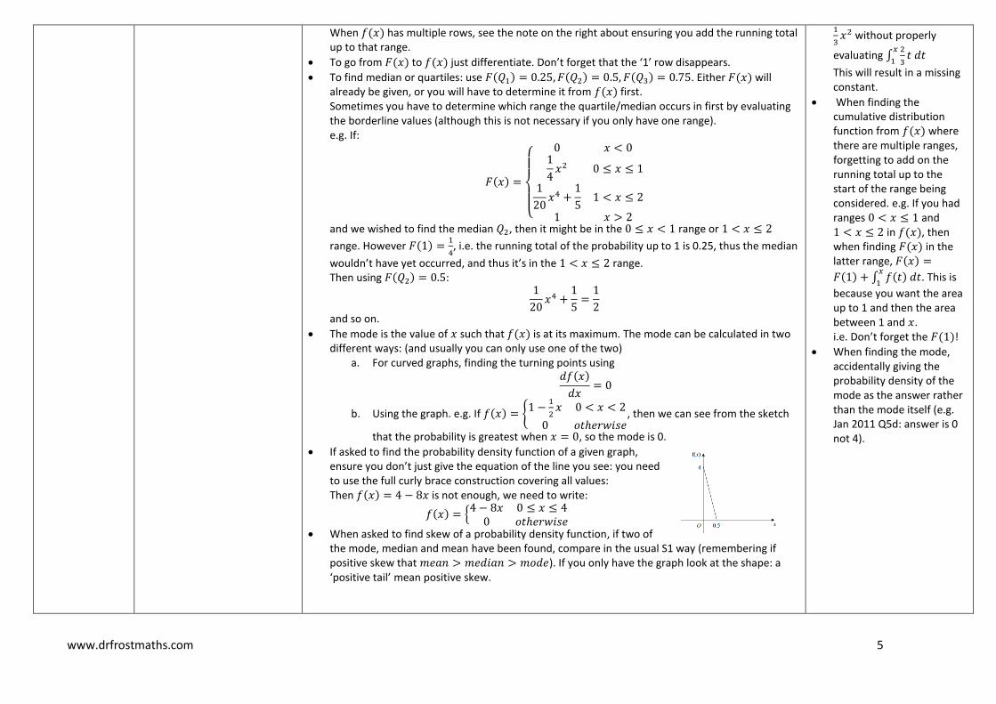
When ( ) has multiple rows, see the note on the right about ensuring you add the running total up to that range.

To go from ( ) to ( ) just differentiate. Don’t forget that the ‘1’ row disappears.

To find median or quartiles: use ( ) ( ) ( ) . Either ( ) will already be given, or you will have to determine it from ( ) first. Sometimes you have to determine which range the quartile/median occurs in first by evaluating the borderline values (although this is not necessary if you only have one range). e.g. If:

( )

{

and we wished to find the median , then it might be in the range or

range. However ( )

, i.e. the running total of the probability up to 1 is 0.25, thus the median

wouldn’t have yet occurred, and thus it’s in the range. Then using ( ) :

and so on.

The mode is the value of such that ( ) is at its maximum. The mode can be calculated in two different ways: (and usually you can only use one of the two)

a. For curved graphs, finding the turning points using ( )

b. Using the graph. e.g. If ( ) {

, then we can see from the sketch

that the probability is greatest when , so the mode is 0.

If asked to find the probability density function of a given graph, ensure you don’t just give the equation of the line you see: you need to use the full curly brace construction covering all values: Then ( ) is not enough, we need to write:

( ) {

When asked to find skew of a probability density function, if two of the mode, median and mean have been found, compare in the usual S1 way (remembering if positive skew that ). If you only have the graph look at the shape: a ‘positive tail’ mean positive skew.

without properly

evaluating ∫

This will result in a missing constant.

When finding the cumulative distribution function from ( ) where there are multiple ranges, forgetting to add on the running total up to the start of the range being considered. e.g. If you had ranges and in ( ), then when finding ( ) in the latter range, ( )

( ) ∫ ( )

. This is

because you want the area up to 1 and then the area between 1 and . i.e. Don’t forget the ( )!

When finding the mode, accidentally giving the probability density of the mode as the answer rather than the mode itself (e.g. Jan 2011 Q5d: answer is 0 not 4).

www.drfrostmaths.com 6

4 – Continuous Uniform Distribution

Find the probability of a range for a continuous uniform distribution, e.g. ( ) or ( ).

Sketch the probability function of a continuous uniform distribution.

Find the mean or variance of a continuous uniform distribution:

Find the and of ( ) when the mean and variance of the distribution is given.

Be able to calculate ( )

The probability calculated from a uniform distribution may be fed into a Binomial distribution.

If ( ) then:

( )

( ) ( )

I remember the variance as “a twelfth of the squared difference”.

Suppose ( ) and ( ) and ( ) where and are unknown. Then:

( )

We can then solve these simultaneously.

The key is just remembering the area of the rectangle (when you sketch the p.d.f.) is 1. Therefore

if ( ) then since the width is 2, the height is clearly

. We would specify the probability

density function as:

( ) {

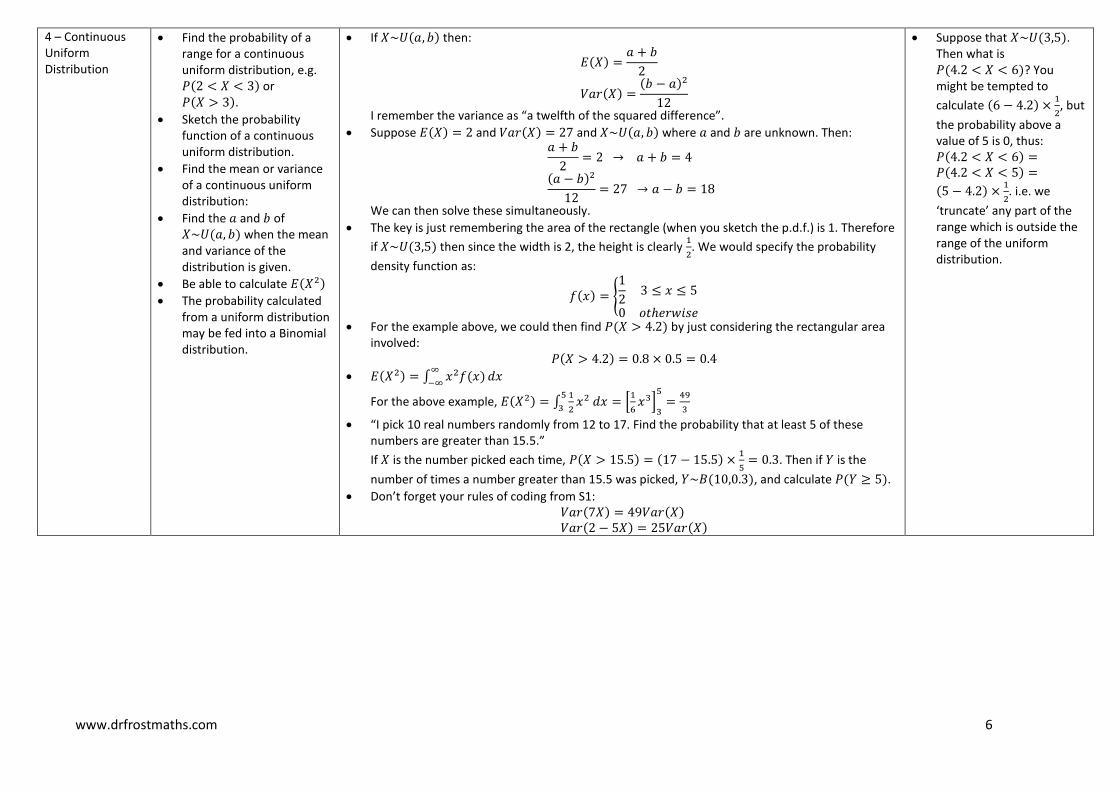
For the example above, we could then find ( ) by just considering the rectangular area involved:

( )

( ) ∫ ( )

For the above example, ( ) ∫

[

]

“I pick 10 real numbers randomly from 12 to 17. Find the probability that at least 5 of these numbers are greater than 15.5.”

If is the number picked each time, ( ) ( )

. Then if is the

number of times a number greater than 15.5 was picked, ( ), and calculate ( ).

Don’t forget your rules of coding from S1: ( ) ( ) ( ) ( )

Suppose that ( ). Then what is ( )? You might be tempted to

calculate ( )

, but

the probability above a value of 5 is 0, thus: ( ) ( )

( )

. i.e. we

‘truncate’ any part of the range which is outside the range of the uniform distribution.

www.drfrostmaths.com 7

5 – Normal Approximations

Be able to approximate a Binomial Distribution using a Normal Distribution.

Be able to approximate a Poisson Distribution using a Normal Distribution.

Be able to approximate a Binomial Distribution using a Poisson Distribution.

Be able to give the conditions under which such approximations can be made.

Justify why we need continuity corrections.

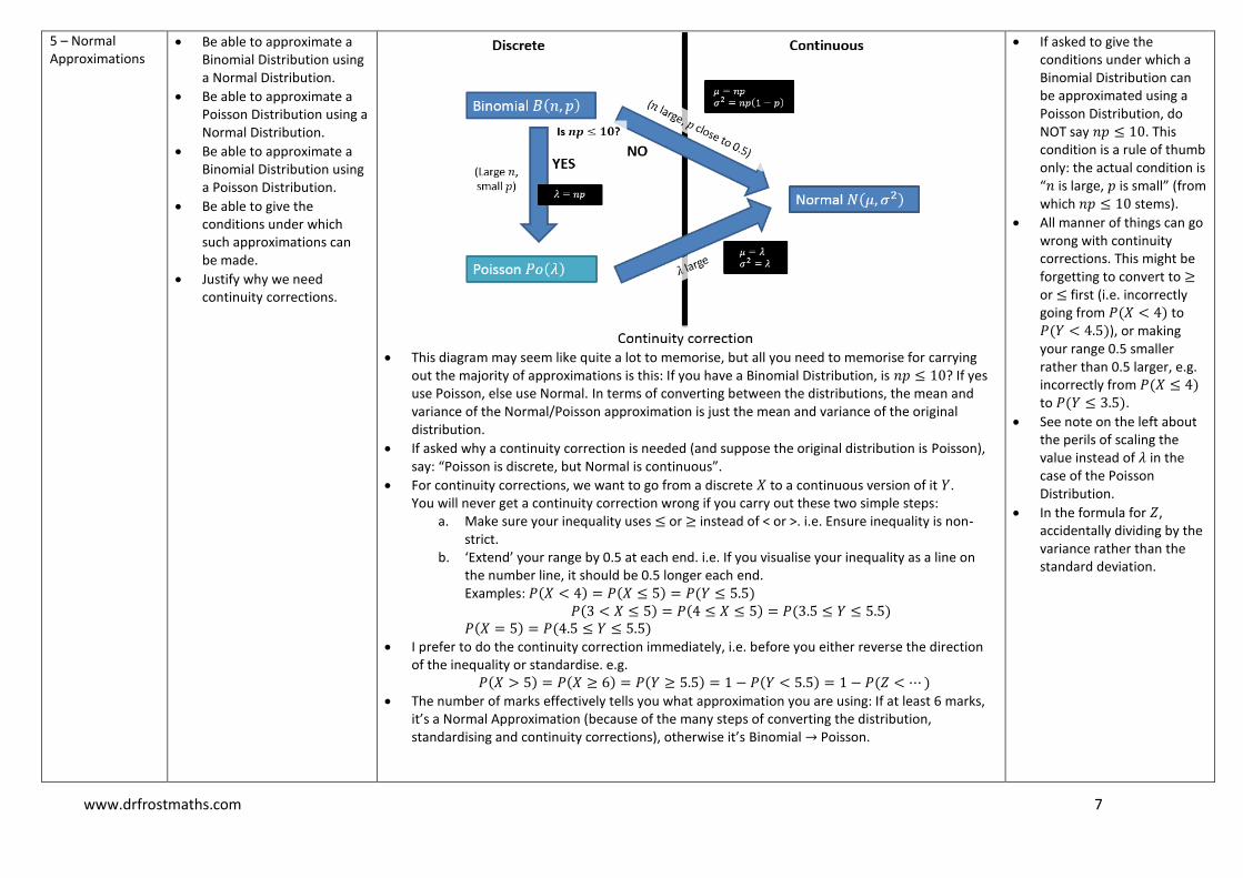
This diagram may seem like quite a lot to memorise, but all you need to memorise for carrying

out the majority of approximations is this: If you have a Binomial Distribution, is ? If yes use Poisson, else use Normal. In terms of converting between the distributions, the mean and variance of the Normal/Poisson approximation is just the mean and variance of the original distribution.

If asked why a continuity correction is needed (and suppose the original distribution is Poisson), say: “Poisson is discrete, but Normal is continuous”.

For continuity corrections, we want to go from a discrete to a continuous version of it . You will never get a continuity correction wrong if you carry out these two simple steps:

a. Make sure your inequality uses or instead of < or >. i.e. Ensure inequality is non-strict.

b. ‘Extend’ your range by 0.5 at each end. i.e. If you visualise your inequality as a line on the number line, it should be 0.5 longer each end. Examples: ( ) ( ) ( )

( ) ( ) ( ) ( ) ( )

I prefer to do the continuity correction immediately, i.e. before you either reverse the direction of the inequality or standardise. e.g.

( ) ( ) ( ) ( ) ( )

The number of marks effectively tells you what approximation you are using: If at least 6 marks, it’s a Normal Approximation (because of the many steps of converting the distribution, standardising and continuity corrections), otherwise it’s Binomial Poisson.

If asked to give the conditions under which a Binomial Distribution can be approximated using a Poisson Distribution, do NOT say . This condition is a rule of thumb only: the actual condition is “ is large, is small” (from which stems).

All manner of things can go wrong with continuity corrections. This might be forgetting to convert to or first (i.e. incorrectly going from ( ) to ( )), or making your range 0.5 smaller rather than 0.5 larger, e.g. incorrectly from ( ) to ( ).

See note on the left about the perils of scaling the value instead of in the case of the Poisson Distribution.

In the formula for , accidentally dividing by the variance rather than the standard deviation.

www.drfrostmaths.com 8

Example Normal Approximation: “The number of houses sold by an estate agent follows a Poisson distribution, with a mean of 2 per week. The estate agent will receive a bonus if he sells more than 25 houses in the next 10 weeks. Use a suitable approximation to estimate the probability that the estate agent receives a bonus.”

a. Note first that you might be tempted to scale the 25 houses in 10 weeks to 5 houses in 2 weeks and stick with the original . The catastrophic flaw in doing this is that the continuity correction affects the range differently depending on whether you’re using the original or scaled value. If not scaling: ( ) ( ) ( ) If scaling: ( ) ( ) ( ) In the latter incorrect case the 0.5 has a greater effect on the smaller value of 6 compared with the larger value of 26, so the probability will be too high.

b. Step 1: Determine what approximation to use. In this example we have a Poisson Distribution, which always goes to Normal. If it were Binomial, you’d first determine if .

c. Step 2: Identify original distribution. As discussed, we scale (rather than the 25), so: ( )

d. Step 3: Write the approximation, potentially with reference to a new continuous variable which is the continuous version of , i.e.: ( ) As discussed, use the mean and variance of the original distribution.

e. Step 4: If necessary, carry out continuity correction to get a probability in terms of : ( ) ( ) ( )

f. Step 5: Use your S1 knowledge and find the probability by first standardising. Don’t forget that you’re dividing by the standard deviation, not the variance:

( ) (

√ ) ( )

( ) 6 – Populations and Samples

Be able to define key terms such as ‘sampling distribution’, ‘sampling frame’, ‘population’, ‘sample’, ‘statistic’.

Be able to describe what the population is or sampling frame is given the context, and identify reasons for differences between the two.

Be able to list possible samples.

Be able to calculate the

Key definitions: a. Statistic: “A random variable (1) which is some function of the sample and not

dependent on any population parameters (1)” - I think the ‘random variable’ bit is a bit pernicious (as does Wikipedia), but c’est la vie! If 1 mark, the second part is important.

b. ‘Population’: The collection of all items. c. ‘Sample’: Some subset of the population which is intended to be representative of the

population. d. ‘Census’: When the entire population is sampled. e. ‘Sampling unit’: Individual member or element of the population or sampling frame. f. ‘Sampling frame’: A list of all sampling units or all the population. g. Sampling distribution: All possible samples are chosen from a population (1); the values

of a statistic and the associated probabilities is a sampling distribution (1).

It’s important you get your head around what the sampling distribution actually is: It gives the distribution over possible values of the statistic as we take different samples. So if for example

When finding the sampling distribution, forgetting that different orderings are different possibilities, e.g. (1,1,2) and (1,2,1) should both be considered.

Even though you can subtract from 1 to find the last probability in your sampling distribution, if you have time, you might want to calculate it ‘the long way’ to check your answer, as probabilities

www.drfrostmaths.com 9

sampling distribution for a variety of statistics, such as median (very common!), range, maximum and mode.

Be able to identify when the sampling distribution is a Binomial Distribution or otherwise, and specify this distribution.

the statistic was the ‘range’ of the sample, then this range is likely to vary as we take different samples. As these ranges vary across samples, it forms a distribution.

The sampling frame is the list of things in the population that are available for sampling, e.g. “The ID numbers”, “The list of car registration numbers”. The mark scheme seems to particularly like it when you refer to some identifying property of the things in the sampling frame. The sampling frame may be different from the population, because some things in the population may not be available for sampling. e.g. If sampling people who’ve visited a medical practice, “some people may have left the area but hadn’t deregistered”.

When listing outcomes, it helps to be systematic in listing them so you don’t miss any. Note that different orderings count as distinct possibilities. e.g. “You have a large collection of 1p, 2p and 5p coins, and take 3 coins. Find all samples in which the maximum is 5.” We may want to first list the possibilities where 5 appears once, 5 appears twice, and so on…” (5,1,1), (1,5,1), (1,1,5), (5,1,2), (5,2,1), (1,5,2), (2,5,1), (1,2,5), (2,1,5), (5,2,2), (2,5,2), (2,2,5), (5,5,1), (5,1,5), (1,5,5), (5,5,2), (5,2,5), (2,5,5), (5,5,5)

e.g. “A bag contains a large number of 1p and 2p coin, of which 40% are 1p and 60% are 2p. A sample of 2 coins. Find the sampling distribution of the sample maximum.” When finding the sampling distribution, it may help to have a table as follows to organise your working, such that the outcomes for each possible value of the statistic are grouped:

Possibilities Statistic (Maximum) Probability

(1,1) 1

(1,2), (2,1), (2,2) 2

Notice that we didn’t need to do any complicated calculation for the last probability, because it was just 1 minus the others! Had we had to calculate it fully, then

On the rare occasion you get a question asking for the sampling distribution, where you don’t actually have to do any calculation, but just have to consider what well-known distribution you get as the sample varies: “A factory produces components. Each component has a unique identity number and it is assumed that 2% of the components are faulty. On a particular day, a quality control manager wishes to take a random sample of 50 components. A statistic represents the number of faulty components in the sample. Specifying the sampling distribution of .” We know a sampling distribution is the possible values of the statistic as we take different samples of 50 light bulbs. If the statistic is the count of light bulbs, we can see this count varies Binomially between 0 and 50. Thus ( )

should obviously all add up to 1.

www.drfrostmaths.com 10

7 – Hypothesis Testing

Be able to define key terms such as ‘critical region’, ‘hypothesis test’, ‘significance level of a test’.

Determine a critical region (one or two ranges depending on whether one or two tailed)

Understand when we need the probability to be strictly within the significance level, and when to be close to it as possible either side.

Be able to calculate the ‘actual level of significance’.

Carry out a hypothesis test involving Binomial and Poisson distributions.

Carry out a hypothesis test where a normal approximation is required.

Key terms whose definitions you need to remember: a. Critical Region: The range of values such that the null hypothesis is rejected. b. Hypothesis Test: a procedure to examine a value of a population parameter proposed

by the null hypothesis c. Significance level: “the probability of rejecting if is true”, or “the probability of

incorrectly rejecting ”.

The “or more extreme” thing often confuses people: is “more extreme” below the value or above it? We can always tell this by what side of the mean we’re on. If and we’re interested in seeing 10 hits to a website “or more extreme”, then since 10 is above the mean of 7, clearly we want “10 or above” to get the tail. Ensure “10 or above” is not .

Identifying the critical values from a table: Firstly, note if the test is one-tailed (involving or ) or two-tailed (involving ), as you need to halve the significance level each side in the latter case. At the left tail, find the closest value under the significance level (or half it) in the table, or if you are explicitly told to use the closest value to the significance level, do that. This is the lower end of the critical region. However, at the right tail, first find the closest value above it (or again if explicitly told, the closest value either side), but then go one above it. This is the critical value. Example: Under the null hypothesis ( ). For a two-tailed test with significance level 5%, what are the critical values? Looking at the tables, at left end , and at right end, closest value with probability above 0.975 is 7, thus going one above . If we had been asked for the ‘closest value’ to 0.025 and 0.975, then we’d then get and instead. It is vitally important you specify the probability of being in each tail to evidence that you have used the table, e.g. “ ( )

For the critical region, don’t forget to provide a lower limit or upper limit in the case of the Binomial Distribution, as the outcomes are finite. For the previous example: . Mark schemes usually condone the lack of , but don’t take any chances.

The actual level of significance is the actual probability of being in the critical region. You should have already written out the probabilities of being in each part of the critical region, so it’s then just a case of adding the two probabilities.

The mark scheme for a hypothesis test without a normal approximation is as follows: a. Specifying and (1 mark) b. Specifying the distribution for under the null hypothesis, e.g. ( ) (1 mark)

The or will be your population parameter under the null hypothesis. c. 2 marks for either: Determining the probability of the observed value or more extreme

(e.g. ( ) ( ) or determining the critical region.

Forgetting to halve the significance level for two-tailed tests.

Being one off the critical value (particularly at the right tail). See notes on the left. Pay careful attention to whether it says “use the closest value”, or not.

Getting your continuity correction wrong (see notes for Chapter 5).

www.drfrostmaths.com 11

d. Using your probability to state whether is rejected or not, ensuring you directly compare your probability with significance level. e.g. “0.0723 > 0.05, so not significant ( is not rejected)” (1 mark)

e. Put this conclusion in context. “Bob is not justified in his claim that the rate of flamingo attacks has increased.”

The mark scheme for a hypothesis test with a normal approximation is usually broken down as the following:

a. Specifying and (1 mark) b. Possibly a mark for specifying your distribution of , i.e. ( ) or ( ) c. Specifying the distribution of for your normal approximation, ( ) (1 mark) d. Doing the continuity correction: ( ) ( ) (1 mark) e. Standardising to get ( ). Note at this stage vs does not matter as variable is

continuous. (1 mark) f. As above, 2 marks for your two-part conclusion.

Note that it is possible for the actual level of significance to be greater than the level of significance, if you were asked to find the closest value to 0.025/0.975, etc rather than those strictly below/above these values.

www.drfrostmaths.com 12

Wordy/interpretation questions:

Definitions (see the respective chapter notes above):

Statistic, population, census, sampling frame, sampling unit, sampling

distribution, critical region, hypothesis test, significance level.

Modelling assumptions:

“List the assumptions made when modelling as a Binomial

distribution”. See Chapter 1.

“State two conditions under which a Poisson distribution is a

suitable model to use in statistical work”. See Chapter 2.

(Surprisingly common!) “Describe the skewness of , giving a reason for your

answer.” The mode and mean had previously been calculated in this question

so “Positive skew as ”. 1 mark for skew type, 1 for reason.

Approximation related:

“Write down the conditions under which the Poisson distribution

can be used as an approximation to the Binomial distribution.”

is large

“Write down the two conditions needed to approximate the

Binomial distribution by the Poisson distribution.”

is large, is small (NOT )

“Write down which of the approximations used in part (a) is the

most accurate estimate of the probability [One was Poisson, one

Binomial]. You must give a reason for your answer.”

Normal approximation (1) because is large and close to half (1).

OR Normal because

“State the probability of incorrectly rejecting H0 using this critical region.”

Add the probabilities of your critical region(s).

[Given that is a continuous variable] “Determine ( )”. Answer is 0.

“Identify a sampling frame.”

See notes on Chapter 6. Remember the mark scheme likes reference to an

‘identifier’, e.g. “list of unique identification numbers of the cookers.”

[In context of cookers being tested] “Give one reason, other than to save

time and cost, why a sample is taken rather than a census.”

There would be no cookers left to sell (i.e. the idea that testing something in a

sample destroys it/makes it unsellable).

“Identify the sampling units”. (Using above example) A cooker

“A researcher took a sample of 100 voters from a certain town and asked

them who they would vote for in an election. The proportion who said they

would vote for Dr Smith was 35%. State the population and the statistic in

this case. What do you understand by the sampling distribution of this

statistic.”

Population is the residents of the town. Statistic is percentage/proportion

who vote for Dr Smith. Sampling distribution here is number of people who

voted for Dr Smith in all possible samples of 100.

[List of possible statistics given] “State, giving a reason which of the following

is not a statistic based on this sample.”

The one involving the and , because these are population parameters,

whereas a statistic must be based on the sample only.

“Suggest a suitable model to describe the number of vehicles passing the

fixed point in a 15 s interval.” ( ) (depending on what the average

rate in the question is, which often you have to

scale)

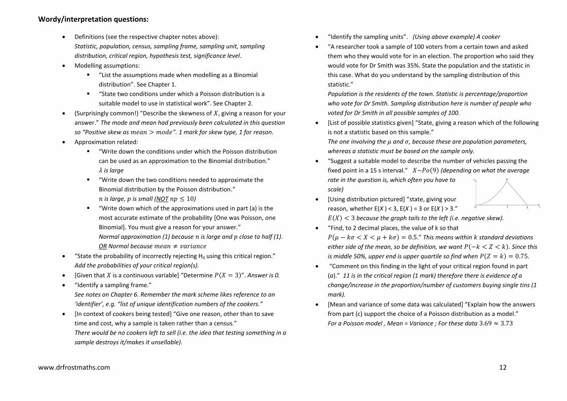
[Using distribution pictured] “state, giving your

reason, whether E(X ) < 3, E(X ) = 3 or E(X ) > 3.”

( ) because the graph tails to the left (i.e. negative skew).

“Find, to 2 decimal places, the value of k so that

( ) .” This means within standard deviations

either side of the mean, so be definition, we want ( ). Since this

is middle 50%, upper end is upper quartile so find when ( ) .

“Comment on this finding in the light of your critical region found in part

(a).” 11 is in the critical region (1 mark) therefore there is evidence of a

change/increase in the proportion/number of customers buying single tins (1

mark).

[Mean and variance of some data was calculated] “Explain how the answers

from part (c) support the choice of a Poisson distribution as a model.”

For a Poisson model , Mean = Variance ; For these data