Sachin Kumar Porandla Advisor Dr. Wenzhong Gao Optimization of Hybrid Powertrain using DIRECT Algorithm POWERTRAIN DESIGN GROUP MEETING #5

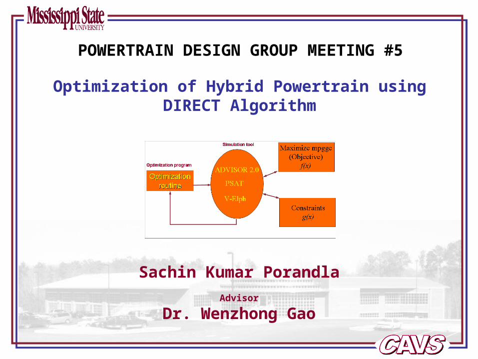
Sachin Kumar Porandla

Advisor

Dr. Wenzhong Gao

Optimization of Hybrid Powertrain using DIRECT Algorithm

POWERTRAIN DESIGN GROUP MEETING #5

Page 2 of 14Intelligent Powertrain Design

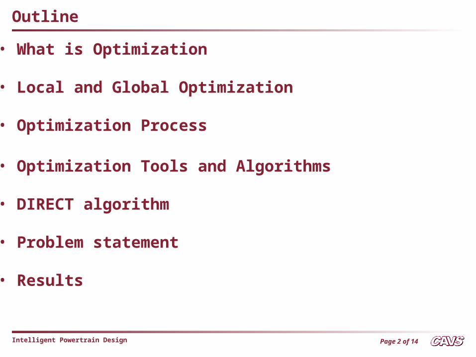
Outline

• What is Optimization

• Local and Global Optimization

• Optimization Process

• Optimization Tools and Algorithms

• DIRECT algorithm

• Problem statement

• Results


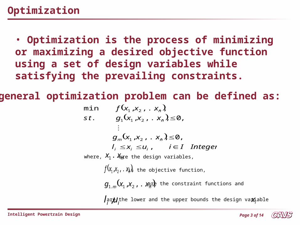
Optimization

• Optimization is the process of minimizing or maximizing a desired objective function using a set of design variables while satisfying the prevailing constraints.

IntegerIiuxl

xxxg

xxxgts

xxxf

iii

nm

n

n

,

,0,...,,

,0,...,,..

,...,,min

21

211

21

nxx ...1

nxxxf ,...,, 21

nm xxxg ,...,, 21..1

ii ul , ix

A general optimization problem can be defined as:

where, are the design variables,

is the objective function,

are the constraint functions and

are the lower and the upper bounds the design variable


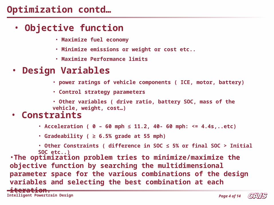
• Constraints• Acceleration ( 0 – 60 mph ≤ 11.2, 40- 60 mph: <= 4.4s,..etc)

• Gradeability ( ≥ 6.5% grade at 55 mph)

• Other Constraints ( difference in SOC ≤ 5% or final SOC > Initial SOC etc..)

Optimization contd…

• Objective function• Maximize fuel economy

• Minimize emissions or weight or cost etc..

• Maximize Performance limits

• Design Variables• power ratings of vehicle components ( ICE, motor, battery)

• Control strategy parameters

• Other variables ( drive ratio, battery SOC, mass of the vehicle, weight, cost…)

•The optimization problem tries to minimize/maximize the objective function by searching the multidimensional parameter space for the various combinations of the design variables and selecting the best combination at each iteration.


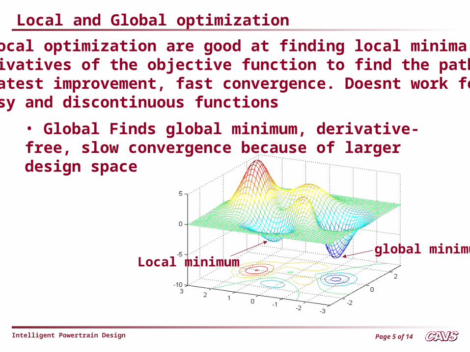
Local minimumglobal minimum

Local and Global optimization

• Local optimization are good at finding local minima, useDerivatives of the objective function to find the path ofgreatest improvement, fast convergence. Doesnt work fornoisy and discontinuous functions

• Global Finds global minimum, derivative-free, slow convergence because of larger design space


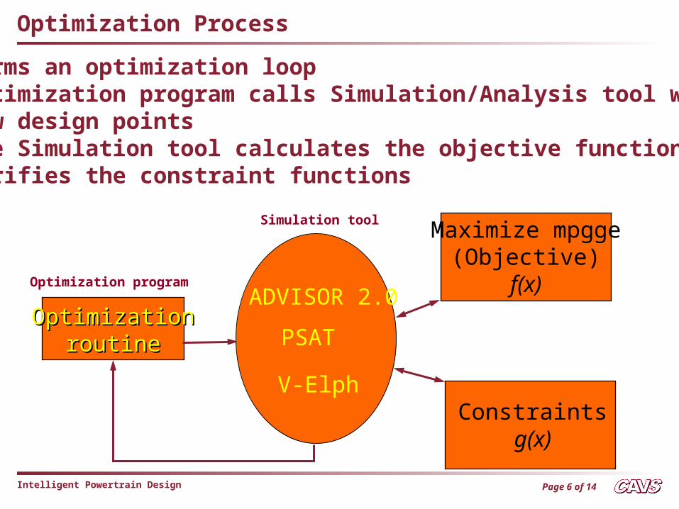
Optimization Process

OptimizationOptimizationroutineroutine

Maximize mpgge(Objective)

f(x)

Constraintsg(x)

• Forms an optimization loop • Optimization program calls Simulation/Analysis tool with new design points• The Simulation tool calculates the objective function and verifies the constraint functions

ADVISOR 2.0

PSAT

V-Elph

Optimization program

Simulation tool


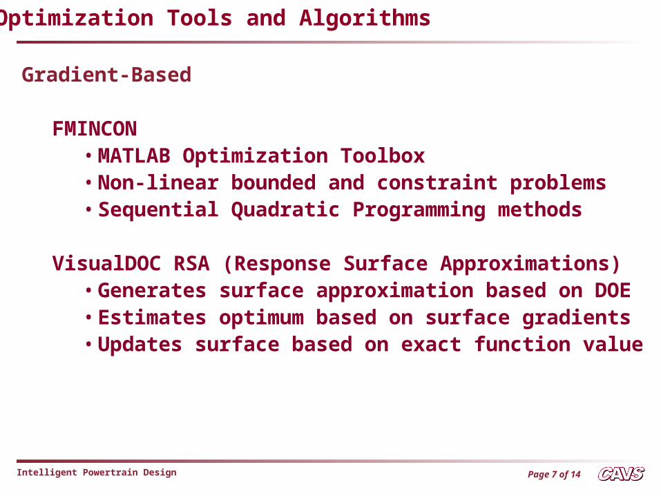
Gradient-Based

FMINCON• MATLAB Optimization Toolbox • Non-linear bounded and constraint problems• Sequential Quadratic Programming methods

VisualDOC RSA (Response Surface Approximations)• Generates surface approximation based on DOE• Estimates optimum based on surface gradients• Updates surface based on exact function value

Optimization Tools and Algorithms


VisualDOC DGO (Direct Gradient Optimization)Applies Sequential Quadratic Programming methods to function values to determine gradients and search direction

iSIGHT• Offers a wide variety of algorithms and solution methods to choose from. Two key features of this tool are 1) its flexibility in defining linkages between multiple programs, and 2) the ability to combine multiple solution methods in series or parallel to solve a specific problem.

• Provides response surface visualization tools that allow the user to explore the impacts of design parameters manually based on design-of-experiments based approximation.

Tools and Algorithms contd…


DIRECT algorithm

DIRECT : DIvided RECTangles

• a global optimization algorithm

• a modification of the standard Lipschitzian approach that eliminates the need to specify the Lipschitz constant

•Lipschitz constant is a weighing parameter, which decides the emphasis on the global and the local search

•eliminates the use of Lipschitz constant by searching all possible values for the Lipchitz constant thus putting a balanced emphasis on both the global and local search.


•The algorithm begins by scaling the design box to a n-dimensional unit hypercube. DIRECT initiates its searchby evaluating the objective function at the center point ofthe hypercube

• DIRECT then divides the potentially optimalhyperrectangles by sampling the longest coordinatedirections of the hyperrectangle and trisecting based onthe directions with the smallest function value until the global minimum is found

• Sampling of the maximum length directions preventsboxes from becoming overly skewed and trisecting in thedirection of the best function value allows the biggestrectangles contain the best function value. This strategyincreases the attractiveness of searching near points withgood function values

DIRECT algorithm contd..



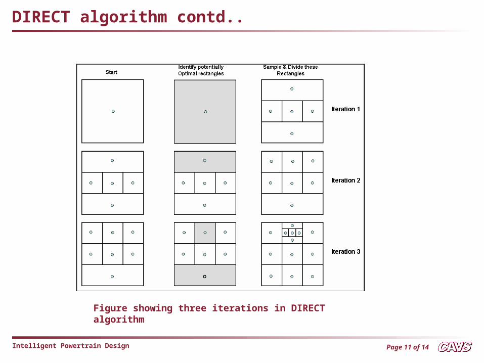
Figure showing three iterations in DIRECT algorithm


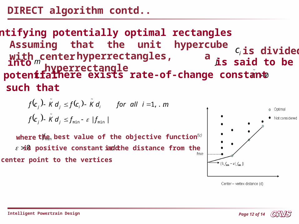
Identifying potentially optimal rectangles

icm j

0~

K

Assuming that the unit hypercube with center is divided hyperrectangles, a hyperrectangle

such that

intopotential

is said to beif there exists rate-of-change constant

||

,...,1

minmin

~

~~

ffdKcf

miallfordKcfdKcf

jj

iijj

minf

0 d

where the best value of the objective function

is positive constant and is the distance from the

center point to the vertices



•The first equation forces the selection of the rectangles in the lower right convex hull of dots and the second equation insists that the obtained function value exceeds the current best function value by a nontrivial amount.

•This prevents the algorithm from becoming too local, wasting precious function evaluations in search of smaller function improvements. The parameter introduced balances the local and global search.



1. Normalize the search space to be the unit hypercube. Let c1 be the center point of this hypercube and evaluate f(c1).

2. Identify the set S of potentially optimal rectangles (those rectangles defining the bottom of the convex hull of a scatter plot of rectangle diameter versus f(ci) for all rectangle centers ci)

3. Choose any rectangle r Є S

4. For the rectangle r:

4a. Identify the set I of dimensions with the maximum

side length. Let δ equal one-third of this maximum side length.



4b. Sample the function at the points c±δei for all i I, where c is ∈the center of the rectangle and ei is the ith unit vector.

4c. Divide the rectangle containing c into thirds along the dimensions in I, starting with the dimension with the lowest value of f(c ± δei) and continuing to the dimension with the highest f(c ± δei).

minx

minf

5. Update S. Set S = S – {r}. If S is not empty, go to Step

3. Otherwise go to Step 6.

6. Iterate. Report the results of this iteration, and then go

to Step 2.

7. Terminate. The optimization is complete. Report the and and stop.



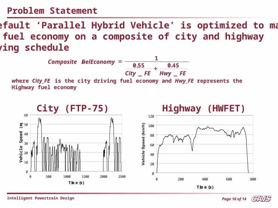
• A default ‘Parallel Hybrid Vehicle’ is optimized to maximize the fuel economy on a composite of city and highway driving schedule

where City_FE is the city driving fuel economy and Hwy_FE represents the Highway fuel economy

FEHwyFECity

uelEconomyComposite F

_45.0

_55.0

1

0

10

20

30

40

50

60

0 500 1000 1500 2000 2500

Time (s)

Veh

icle

Sp

eed

(m

ph

)

0

20

40

60

80

100

120

0 200 400 600 800

Time (s)

City (FTP-75) Highway (HWFET)

Problem Statement


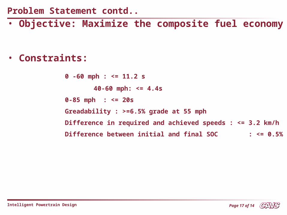
• Objective: Maximize the composite fuel economy

• Constraints:

0 -60 mph : <= 11.2 s

40-60 mph: <= 4.4s

0-85 mph : <= 20s

Greadability : >=6.5% grade at 55 mph

Difference in required and achieved speeds : <= 3.2 km/h

Difference between initial and final SOC : <= 0.5%

Problem Statement contd..



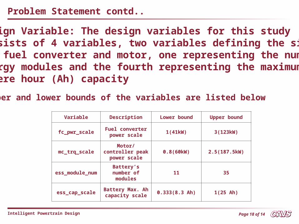
• Design Variable: The design variables for this study consists of 4 variables, two variables defining the size of the fuel converter and motor, one representing the number energy modules and the fourth representing the maximum Ampere hour (Ah) capacity

• Upper and lower bounds of the variables are listed below

Variable Description Lower bound Upper bound

fc_pwr_scaleFuel converter

power scale1(41kW) 3(123kW)

mc_trq_scaleMotor/controller

peak power scale0.8(60kW) 2.5(187.5kW)

ess_module_numBattery’s number

of modules11 35

ess_cap_scaleBattery Max. Ah capacity scale

0.333(8.3 Ah) 1(25 Ah)



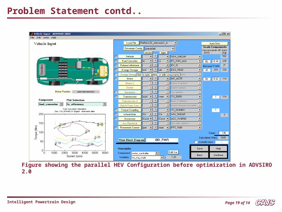
Figure showing the parallel HEV Configuration before optimization in ADVSIRO 2.0


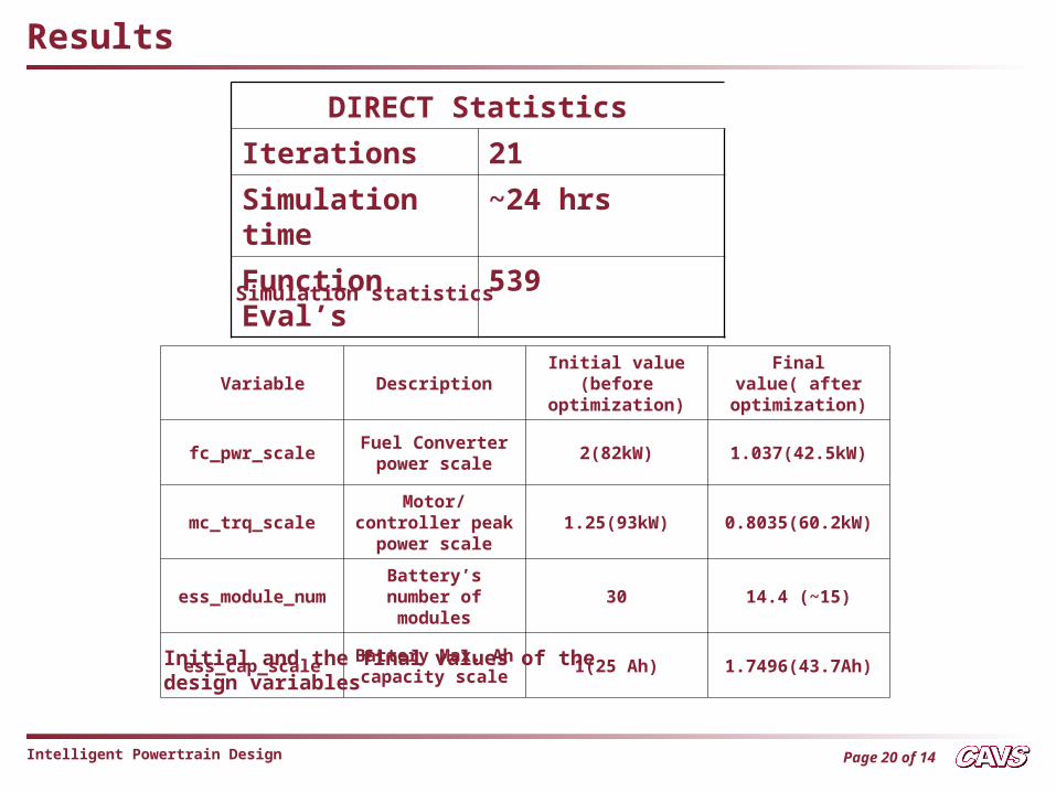
DIRECT Statistics

Iterations 21

Simulation time ~24 hrs

Function Eval’s 539

Variable DescriptionInitial value (before

optimization)Final value( after

optimization)

fc_pwr_scaleFuel Converter

power scale2(82kW) 1.037(42.5kW)

mc_trq_scaleMotor/controller

peak power scale1.25(93kW) 0.8035(60.2kW)

ess_module_numBattery’s number

of modules30 14.4 (~15)

ess_cap_scaleBattery Max. Ah capacity scale

1(25 Ah) 1.7496(43.7Ah)

Results

Initial and the final values of the design variables

Simulation statistics


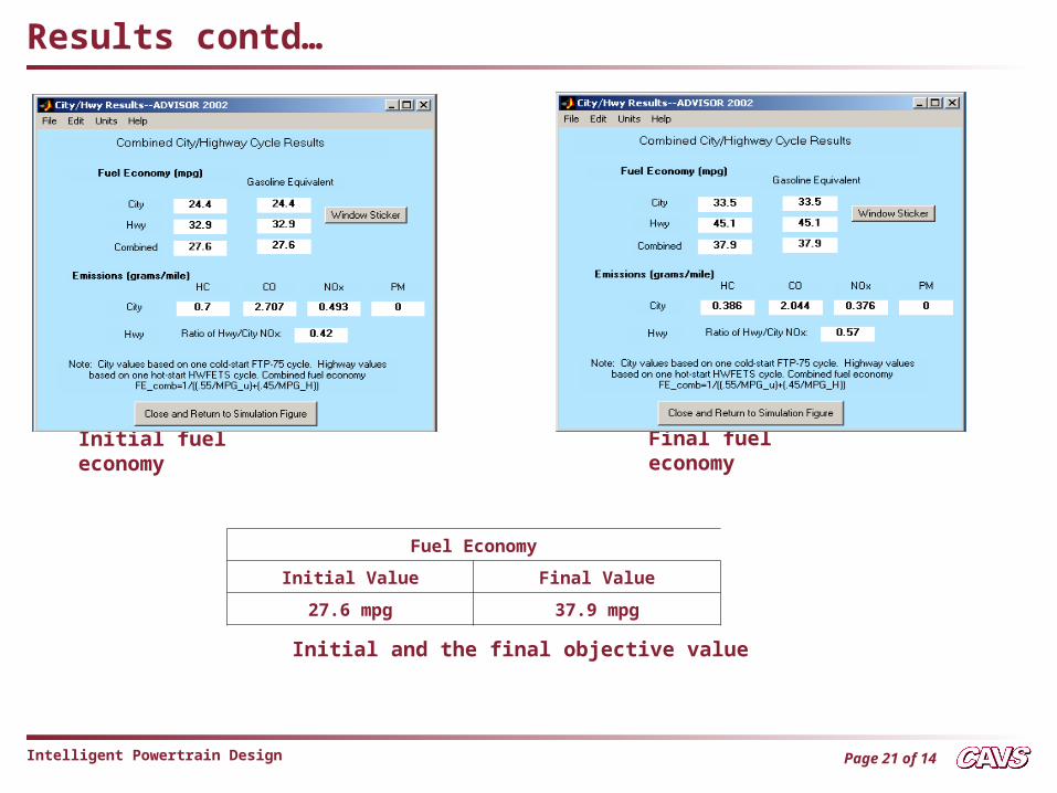
Fuel Economy

Initial Value Final Value

27.6 mpg 37.9 mpg

Results contd…

Initial and the final objective value

Initial fuel economy Final fuel economy


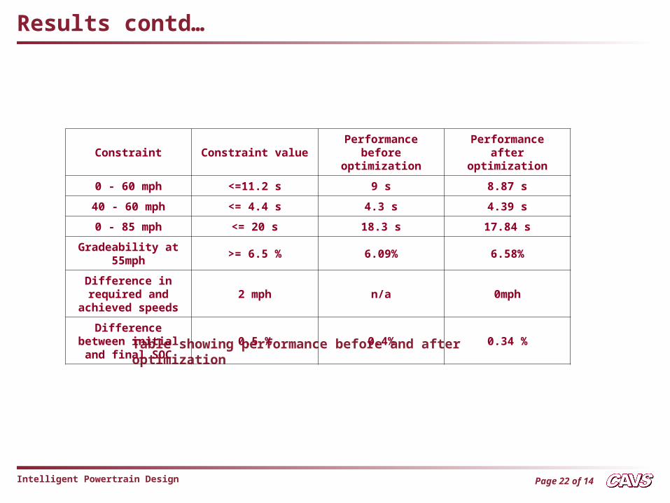
Table showing performance before and after optimization

Constraint Constraint valuePerformance before

optimizationPerformance after

optimization

0 - 60 mph <=11.2 s 9 s 8.87 s

40 - 60 mph <= 4.4 s 4.3 s 4.39 s

0 - 85 mph <= 20 s 18.3 s 17.84 s

Gradeability at 55mph

>= 6.5 % 6.09% 6.58%

Difference in required and

achieved speeds2 mph n/a 0mph

Difference between initial and final SOC

0.5 % 0.4% 0.34 %

Results contd…


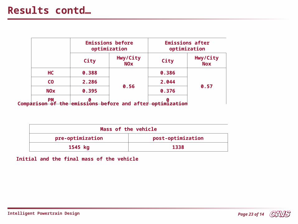
Comparison of the emissions before and after optimization

Mass of the vehicle

pre-optimization post-optimization

1545 kg 1338

Initial and the final mass of the vehicle

Results contd…

Emissions before optimization

Emissions after optimization

City Hwy/City NOx City Hwy/City Nox

HC 0.388

0.56

0.386

0.57CO 2.286 2.044

NOx 0.395 0.376

PM 0 0


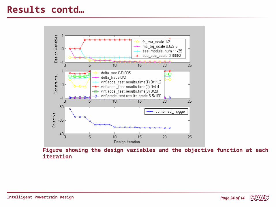
Results contd…

Figure showing the design variables and the objective function at each iteration


References

• Ryan Fellini, Nestor Michelena, Panos Papalambros, and Michael Sasena, “Optimal Design of Automotive

Hybrid Powertrain Systems,” Proceedings of EcoDesign 99 - First Int. Symp. On Environmentally Conscious

Design and Inverse Manufacturing (H. Yoshikawa et al., eds.), Tokyo, Japan, February 1999, pp. 400-405.

• Wipke, K., and Markel, T., ”Optimization Techniques for Hybrid Electric Vehicle Analysis Using ADVISOR,”

Proceedings of ASME, International Mechanical Engineering Congress and Exposition, New York, New York.

(11/11/01-11/16/01)

• M.J.Box, ”A new method of constrained optimization and a comparison with other methods,” Imperial Chemical

Industries Limited, Central Instrument Reseacrh Laboratory, Bozedown House, Whitchurch Hill, Nr. Reading,

Berks 1965.

• D.Jones,” DIRECT Global Optimization Algorithm,” Encyclopedia of Optimization, kluwer Academic Publishers,

2001.

• Report on “Optimal Design of Non-Conventional Vehicles” The University of Michigan, Dept. of Mechanical

Engg., January 19, 2001.

• Haskell R.E., and Jackson C.A., “Tree-Direct: An Efficient Global Optimization Algorithm,” Proc. International

ICSC Symposium on Engineering of Intelligent Systems, University of La Laguna, Tenerife, Spain, February 11-13,

1998.

• Bjorkman, Mattias and Holmstrom, Kenneth, “Global optimization using the DIRECT Algorithm in MATLAB,”

Advanced Modeling and optimization, Vol. 1, No. 2, 1999.

• Jones, D.R., Perttunen, C.D., Stuckman, B.E. ,”Lipschitzian Optimization without Lipschitz Constant,” Journal of

Oprtimization Theory and Applications, Vol. 79, No. 1, October 1993.

• Finkel D.E., and Kelley C.T., “Convergence Analysis of the DIRECT Algorithm,” N. C. State University Center for

Research in Scientific Computation Tech Report number CRSC-TR04-28, July, 2004.

Documents

Sachin Kumar Porandla Advisor Dr. Wenzhong Gao Optimization of Hybrid Powertrain using DIRECT Algorithm POWERTRAIN DESIGN GROUP MEETING #5