SADC SECRETARIAT EUROPEAN DEVELOPMENT FUND

Promotion of Regional Integration in the SADC Livestock Sector (PRINT Livestock Project)

9 ACP SAD 002

Report of a Mission on LIMS Livestock Information and Management System: Improvement of LIMS demographic data collection and use (Dip Tank Crush Pen DT/CP aggregated model) for the SADC APVM (Animal

Production Veld & Marketing) and the EIS (Epidemiology and Informatics) Sub committees of SADC

By

Dr. Matthieu LESNOFF CIRAD

PRINT Report N°: ML-Demog-LIMS-BW- 06-2009

SADC Secretariat FANR Directorate, Portion 116 Millenium Office Park Kgale View P/Bag 0095 Gaborone Botswana 15th–25th June 2009

Acknowledgments The consultant would like to thank the staff members of the SADC PRINT project who participated in the discussions and provided valuable information. Special thanks go to Dr Pascal Bonnet for facilitating the organisation of the mission and to provide access to all documents needed.

Index 1. Objectives and activities of the mission............................................................................4

1.1. Objectives.................................................................................................................4 1.2. Specific activities ......................................................................................................4

1.2.1. Stage 1 – Mission preparation ..........................................................................4 1.2.2. Stage 2 – Intervention in SADC-Botswana.......................................................5

2. Description of the actual DT/CP system...........................................................................6 2.1. General principles.....................................................................................................6 2.2. Examples of DT/CP demographic forms used in SADC countries .........................12

3. Theoretical background on livestock demographic methods..........................................19 3.1. Introduction.............................................................................................................19 3.2. Basic demographic parameters ..............................................................................19

3.2.1. Definitions .......................................................................................................19 3.2.2. Calculations of annual hazard rates ...............................................................22

3.3. Global demographic indicators ...............................................................................23 3.3.1. Dynamics ........................................................................................................23 3.3.2. Production.......................................................................................................23

3.4. Simulations with mathematical demographic models .............................................24 3.4.1. General principles...........................................................................................24 3.4.2. Variable versus constant demographic environment ......................................25 3.4.3. Practical applications ......................................................................................26

4. Recommendations..........................................................................................................28 4.1. Introduction.............................................................................................................28 4.2. Data collection at herd level ...................................................................................29

4.2.1. Data collection without animal categorization.................................................29 4.2.2. Data collection with animal categories............................................................29

4.3. Data aggregation at the DT/CP level (spatial aggregation) ....................................32 4.3.1. Situation where the herds of the DT/CP area are surveyed exhaustively ......32 4.3.2. Situation where only a sample of herds is surveyed.......................................32

4.4. Data aggregation over the year (temporal aggregation).........................................32 4.4.1. Case of monthly surveys ................................................................................32 4.4.2. Case of annual surveys ..................................................................................33

4.5. Demographic calculations ......................................................................................33 4.5.1. Preliminaries ...................................................................................................33 4.5.2. Basic demographic parameters ......................................................................34 4.5.3. Global demographic indicators .......................................................................35

4.6. Training on Livestock demographic methods .........................................................35 5. References cited in the report ........................................................................................36 6. Annexes..........................................................................................................................37

6.1. Probabilities and hazard rates in demography .......................................................37 6.2. DYNMOD – A simple MS Excel interface for simulating ruminant livestock demography .......................................................................................................................38

6.2.1. Background.....................................................................................................38 6.2.2. General characteristics ...................................................................................38

6.3. Manual DYNMOD Version 6...................................................................................40

3

1. Objectives and activities of the mission

1.1. Objectives The mission had the general objectives:

- To improve the methodological aspects of the collection and use of LIMS demographic data collected at Dip Tank / Crush Pen level (DT/CP model) in SADC Member States and at SADC regional level;

- To enhance the capability of national livestock departments to understand the

characteristics of their own animal population based on DT/CP data;

- To appraise data quality & completeness and therefore to improve the further interpretation and use of study results using similar quantitative data.

The mission focused on the ruminant livestock (cattle, sheep, goats) and the LIMS “dipping tank/crush pen” (DT/CP) data collection system. The mission is a technical support to the SADC Sub-Committee on Animal Production Veld, Marketing & Genetic resources and to the Sub-Committee on Epidemiology and Informatics regarding their advisory role in the generation and use of quality data on livestock ruminants populations. The recommendations of the consultant have been scrutinized with a view to identifying those that can be addressed through means available to the PRINT Livestock Project or sisters projects at SADC and those that require additional support (possibly from other donors).

1.2. Specific activities The mission’ activities have been implemented in two stages.

1.2.1. Stage 1 – Mission preparation

Prior to the mission in SADC-Botswana, the consultant has:

- Established contact with the CTA of PRINT at SADC secretariat;

- Done a short desk study on material provided: read the LIMS templates and manuals developed for LIMS Module 1 (Livestock population and composition), i.e. the four worksheet templates using four different breakdown models for population counting, as compiled by PRINT and Sub committees in 2008, and taken stock of the way the LIMS application (Module 1) deals with data capture and queries;

- Taken stock of and consulted the other relevant literature assembled (e.g. selected

situation analysis reports for the comparison of census methods in member states), as compiled by PRINT during the situation analysis of SADC Member States and the LIMS adoption missions implemented from 2007 to 2009;

- Started analysing, liaising with the PRINT CTA, the various ways data are collected in

Member states with a particular focus on countries using the DT or CP models (i.e. the collection of animal population data during sanitary interventions be they vaccinations or dipping) and prepare the mission to Botswana;

4

- Considered the other methods used in SADC countries: e.g. agricultural surveys (with sampling), decadal agricultural censuses.

1.2.2. Stage 2 – Intervention in SADC-Botswana

The consultant has (*):

- Formulated guidelines and recommendations on: o Strategies to improve the collection and use of ruminant population DT/CP

data in the SADC region; o Cautious use of ruminant population DT/CP data (from LIMS) in studies; o Methods for calculating demographic parameters derived from DT/CP data.

- Demonstrated and supplied a demographic modelling tool with its learning material,

that can be used for prospective modelling of ruminant populations in the SADC region and based on LIMS data; and document how LIMS data (Module 1) can be used and inputted into such systems (identify opportunities and constraints);

- Produced a report on the consultancy, and provide the necessary hard copy and

electronic documentation;

- Attached the necessary annexes and tools including electronic ones;

- Advised the SADC Livestock unit and the PRINT Livestock Project on an appropriate dissemination and training strategy through the Sub committees of SADC.

(*) Remark: Though planned by PRINT, it was not possible to meet with the authorities of Botswana to debrief them, since most national senior staff were not available at the time of the consultant’ visit to Botswana. PRINT will therefore disseminate and present the results of the consultancy at the APVM sub committee and LTC meetings and also post summary information on the LIMS web site.

5

2. Description of the actual DT/CP system

2.1. General principles For the purpose of the general illustration of the DP/CP population statistical model, one will take a few examples of its use in Swaziland and Lesotho. Spatial resolution of zonal statistics on animal populations In Swaziland the country can be divided in administrative regions which are named “administrative partitions” in LIMS.

Map 1: Regions of Swaziland (Source PRINT)

Moreover, one can use the concept of “Technical partitions” which are thematic divisions of a country according to a particular management, e.g. for livestock and disease issue. The following maps show the veterinary districts and veterinary sub-regions as used by the ministry.

6

Map 2: Veterinary districts in Swaziland (Source PRINT ZAITS study 2009©)

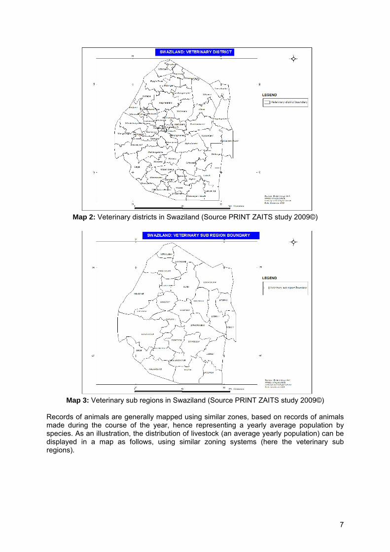
Map 3: Veterinary sub regions in Swaziland (Source PRINT ZAITS study 2009©)

Records of animals are generally mapped using similar zones, based on records of animals made during the course of the year, hence representing a yearly average population by species. As an illustration, the distribution of livestock (an average yearly population) can be displayed in a map as follows, using similar zoning systems (here the veterinary sub regions).

7

Map 4: Livestock distribution in Swaziland (Source PRINT ZAITS study 2009©)

The regular counting of animals, therefore the representation of animal population structure and composition for a given period, is done at a smaller spatial resolution, using management units like dip tanks or crush pens, i.e. when sanitary interventions are carried out, be they vaccinations or dipping. The following figures show the spatial distribution of the dip tank infrastructures in Swaziland, and the DT catchment areas in Lesotho. Dip tanks and similarly crush pens serve as observation units for the purpose of population and demographic surveys. Dip tanks and crush pens can be seen as infrastructures (dot on a map) and as well as zones forming an irregular lattice, when considering their catchment areas, i.e. the surrounding area covering the official list of villages, of farmers and their herds which are assigned the use of such a particular infrastructure.

8

Map 5: Dip Tank distribution in Swaziland (Source PRINT ZAITS study 2009©)

Map 6: Simplified Dip Tank distribution (dots) in Swaziland (Source PRINT)

9

Map 7: Dip Tank distribution and DT catchment areas in Lesotho (Source PRINT Situation analysis study 2007©, based on DVS data)

Temporal resolution for zonal statistics of animal populations

Monthly or weekly dipping in DT

t = 0 1 2 3 4 5 6 7 8 9 10 11 12

months

1 2 3 4 5 6 7 8 9 10 11 12

Year y

Beginning of year y

End of year y

(or, equivalently, beginning of year y+1)Yearly Vaccination Campaign using CP

Figure 1: Frequency of contact for demographic surveys when using vaccination campaign or dipping (Source PRINT Situation analysis studies 2007-08©) In the case of dipping the frequency of the sanitary interventions (at spraying races and dipping tanks) varies according to the seasons (rainy season versus dry) and the country zones (high prevalence of vectors in TBD – tick borne disease - prone areas versus low). In general one can expected a visit by animal at risk, every week or fortnightly. In such an example a monthly average can be done instead of using weekly snapshots of animal population number and composition.

In the case of vaccination it can be yearly (Anthrax) or biannually (FMD vaccination and CBPP for instance). Therefore the frequency of survey and data records regarding the structure of the animal population is varying with the type of intervention. Moreover in some instances young animals may not be presented at such DT or CP though should be accounted for in the animal population structure derived from the animal population survey.

t = 0 1 2 3 4 5 6 7 8 9 10 11 12

months

1 2 3 4 5 6 7 8 9 10 11 12

Year y

Beginning of year y

End of year y

(or, equivalently, beginning of year y+1)

Monthly or weekly dipping

Counting of animals during Round 2 of APE survey Agricultural production estimate in Malawi (March to May - June)

Figure 2: Frequency of contact for demographic surveys when using planned agricultural surveys using other zonal systems (Source PRINT Situation analysis studies 2007-08©, Malawi using EPA Extension Planning Areas). In some country an equivalent system can be described instead of yearly vaccination, with the yearly production estimate, like in Malawi. The zone of interest is no more the DT or CP (smaller zones in general) but an EPA Extension planning area. Ina country which implement movement control every animal (or alternatively batch of animal, herd) leaving an assigned area (DT or CP area) is receiving a movement permit which can be used to derive information of animal leaving or entering an area (transit IN or transit OUT). Movements within a given DT or CP area are considered transfer from a farm to another farm within the zone. This model is scalable to a larger zone (veterinary district. for instance)

11

Figure 3: A simplified zonal statistical system based on DT or CP (in green the DT CP catchment area). At a given date (its frequency varying), animals from neighbouring farms (small dots) are sent (arrow’ flows) to the DT (circle in red) and are being treated at this central infrastructure. Meanwhile counting of animals is done. Some animals may be excluded from the counting related to the DT if they go to another dip tank because of a better accessibility. The aggregation of data at an upper level (all DT of the area) will account for them. New methods to record and timely transfer and analyse data on animal population: In such a model data can be recorded on paper (cf. previous chapter and examples from Member states) and then compiled at an upper level therefore following the classic reporting channel. They may alternatively be recorded on electronic devices like Palm and Smartphones with the tabular files eventually being sent directly to a central computing facility (server). Another example of modernization of the recording process is the use of digital pen which combines a form specially prepared for OCR and a cell phone can send the stroke to a central server where the data is validated and collated. The later is being tested by the PRINT project in collaboration with the TAD’s project and the FAO RCAH. Such an automation of data flow (workflow) is needed when the population data are captured nation wide and with high frequency, e.g. weekly dipping on a country.

2.2. Examples of DT/CP demographic forms used in SADC countries For the purpose of specific illustrations of the questionnaires and datasets used and generated at DP / CP or at other zonal levels, one will take a few examples of its use in Swaziland, Malawi and Lesotho. Such examples of forms used by SADC countries for collecting demographic data on ruminant livestock in DT/CP areas were collected in countries by the PRINT project before the mission. They were analysed during the mission. Selected representative copies of such forms are presented from Figure 4 to Erreur ! Source du renvoi introuvable. as examples. They all corresponded to either monthly or annually retrospective routine surveys.

12

In general, the forms analysed presented inadequate information to calculate fully informative demographic parameters. Therefore the consultant recommends enhancing the national forms following the elements provided in the both forthcoming chapters of this report (Theoretical background and Recommendations).

(a)

13

(b)

Figure 4: Example of a monthly individual DT demographic report form in Swaziland and monthly aggregated DT demographic report form (its aggregate). The form captures the demographic structure of the population at the time of the survey and the movements the last month. Some codes used in the form are defined as follows: CBF=female calves, CBM=male calves, PI=permitted in (animals that are registered in a dipping tank from another dipping tank), PO=permitted out (animals that are deregistered from a dipping tank to move to another dipping tank), D= dead (animals that are deregistered from a dipping tank due to death of natural causes (disease ,unknown, old age), K= killed (animals that are deregistered from a dipping tank due to slaughter).

(a) Form 1: Malawi beef monthly report from an EPA extension planning area

14

(b) Form 2: Malawi Dairy monthly report from an EPA extension area

(c) Form 3: Malawi Goat monthly report from an EPA extension planning area

15

(d) Form 4: Malawi Sheep monthly report from an EPA extension planning area

Figure 5: Beef & Dairy Cattle, Goat, Sheep monthly reporting Forms from an EPA extension planning area in Malawi. The forms capture the demographic structure of the population at the time of the survey and the movements the last month (inputs, outputs transfers).

Figure 6: Example of a monthly DT sales report form in Swaziland. The form captures the sales movements the last month and its destination.

16

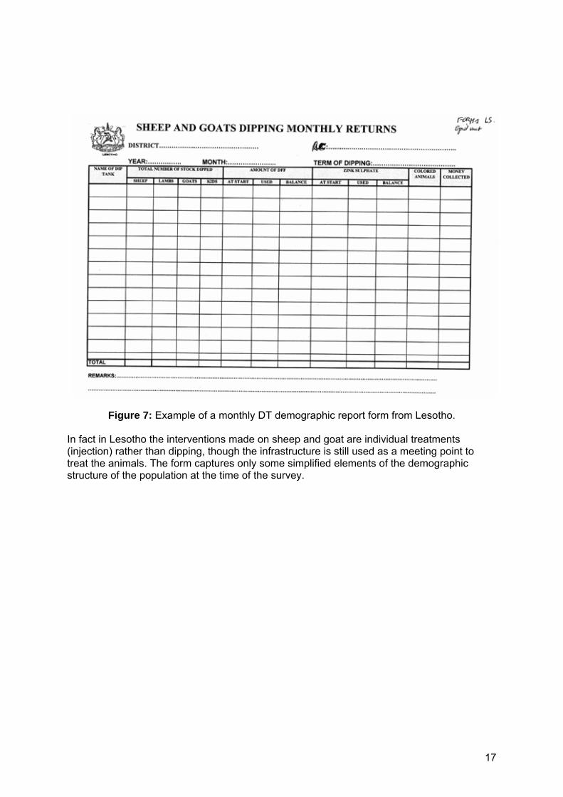
Figure 7: Example of a monthly DT demographic report form from Lesotho. In fact in Lesotho the interventions made on sheep and goat are individual treatments (injection) rather than dipping, though the infrastructure is still used as a meeting point to treat the animals. The form captures only some simplified elements of the demographic structure of the population at the time of the survey.

17

Figure 8: Example of an annual DT demographic reports form in Swaziland (cattle and small stock). The form captures the demographic structure of the population at the time of the survey and the movements the last 12 month.

18

3. Theoretical background on livestock demographic methods

3.1. Introduction Demography is an important trait for characterizing livestock populations, particularly in extensive or semi-extensive tropical farming systems. This chapter presents some main concepts used in ruminant livestock demography. The concepts can be applied to different levels of observation, for instance to farms’ herds or to livestock populations of a DT/CP zone, a district or a country. In the chapter, the term “herd” is used independently of the observation level and can represent farm’s herds or larger populations. The chapter is organized in three parts. The first part presents the basic demographic parameters commonly used to quantify herd demography. The second part presents global indicators, on herd dynamics and production (in terms of number of animals), which summarize the herd demography. The third part introduces the herd demographic models used for implementing projections.

3.2. Basic demographic parameters

3.2.1. Definitions

Basic demographic parameters can be divided in two types:

- The “state variables”, describing the state of the herd at a given time1: o Herd size (number of animals); o Sex-by-age structure;

- The “demographic rates”, describing the demographic events occurring in the herd

during a period of time2: o Natural rates, referring to the natural performances of the herd (reproduction

and mortality); o Management rates, referring to the events directly related to farmers decisions

(slaughtering, sales, purchases, etc.). Many types of demographic rates can be defined depending on the level of details needed by the users. A list of rates adapted to ruminant livestock in extensive or semi-extensive tropical farming systems has been proposed in Lesnoff et al., 2007, 2009 and is presented in Table 1 and Table 2 (see Figure 9 for the corresponding animal life-cycle decomposition). Calculations of herd size, herd sex-by-age structure and prolificacy and mortinatality rates present no difficulty and are not detailed in this chapter. Rates of parturition, abortion, mortality, offtake and intake are more complex to calculate. They can represent either probabilities or hazard rates (See the Annexes section for details on both parameters). In the present report, rate are defined as hazard rates (referred to as “h”) since they are more easy to calculate from DT/CP data than probabilities. They are calculated on an annual basis

1 Such state variables are captured in Module 1 of LIMS 2 Some additional data of LIMS may be used to participate to the estimation of such parameters though imperfectly (e.g. Module 3 on slaughters, Module 10 on mortality)

19

and are assumed to be constant throughout the year. Calculation formulas are presented in the next section. Table 1: List of basic annual demographic rates for tropical ruminant livestock (from Lesnoff et al., 2007, 2009).

Type of rate Name Definition Natural rates Parturition rate Mean number of parturition (delivery) per reproductive female in

the year Abortion rate Mean number of abortion per reproductive female in the year

(an abortion is a gestation which has not reached its end, generating a non-viable offspring)

Prolificacy rate Mean number of offspring (born alive or stillborn) per parturition Mortinatality rate Probability that an offspring is a stillborn (mortinatality is not

included in the natural mortality, which concerns only the offspring born alive)

Rate of females at birth

Probability that an offspring born alive is a female (in practice, this rate is rarely estimated from data and is generally set to 50%)

Mortality rate Rate on which animals die from natural death in the year (natural deaths refer to all types of death except slaughtering. Emergency slaughtering, due for example to sicknesses, are considered as offtake and not as natural mortality)

Management rates

Offtake rate Rate on which animals exit from the herd as offtake (slaughtering, sales, gifts, etc.) in the year

Intake rate Rate on which animals enter in the herd as intake (purchases, gifts, etc.) in the year.

Table 2: Additional list of parameters for tropical ruminant livestock (from Lesnoff et al., 2007, 2009), derived from the basic annual demographic rates above.

Name of rate Definition Net prolificacy rate Mean number of offspring born alive per parturition, calculated

directly or by:

Prolificacy rate * (1 – Mortinatality rate)

Fecundity rate Mean number of offspring (born alive or stillborn) per reproductive female/year, calculated directly or by:

Parturition rate * Prolificacy rate

Net fecundity rate Mean number of offspring born alive per reproductive

female/year, calculated directly or by:

Parturition rate * Net prolificacy rate

20

Reproductive females

ParturitionsAbortions

Births

− Simples

− Twins

− Triplets

− etc.

Born alive

− Females

− Males

Stillborn

Survivals Natural deaths

(2) Parturition rate

(1) Abortion rate

(3) Prolificacy rate

(4) Mortinatality rate

Offtake

Intakes

(6) Mortality rate

(7) Offtake rate

(8) Intake rate

(5) Rate of females at birth

Figure 9: Animal life-cycle used to define the list of the demographic rates in Lesnoff et al. (2007, 2009).

3.2.2.

21

Calculations of annual hazard rates

Annual hazard rates can be calculated globally over the herd or by animal category (sex, age class, etc.). This section considers the global herd. The principle is the same for any animal category. The annual hazard rate of a given demographic event (parturition, death, offtake, etc.) is generally calculated by:

h = m / T, Where:

- m: Number of events occurred in the herd during the year; - T: Time of presence of the animals in the herd during the year (in epidemiology, T is

referred to as the “time at risk” of the animals). In livestock studies, T is rarely calculable from the real animal-times of presence (such data are rarely available in practice). In general, T is approximated by the mean herd size (mean number of animals present in the herd) over the year, following the same principle as in the life-table methods in human demography (Chiang, 1984). For instance, assuming that:

- Monthly data are available; - t=0, 1, 2, 3, etc. represent the beginning of the successive months of the year y (t=0

represents the beginning of year y and t=12 the end of year y or, equivalently, the beginning of year y+1; Figure 10);

- nt represents the herd size (i.e. the number of animals) at time t.

The time T corresponding to year y can be approximated by:

13

12

0∑

==≈ ttn

nT ,

When only annual data are available, T can be approximated by:

2120 nnnT +

=≈ .

22

t = 0 1 2 3 4 5 6 7 8 9 10 11 12

months

1 2 3 4 5 6 7 8 9 10 11 12

Year y

Beginning of year y

End of year y

(or, equivalently, beginning of year y+1)

Figure 10: Notations used for a monthly decomposition of a given year y.

3.3. Global demographic indicators Global indicators can be calculated to summarize the herd demography, in particular on the:

- Annual herd dynamics, i.e. the evolution of the animal stock from years to years; - Annual herd production, i.e. what the animal stock produces per year in term of

number of animals. This section presents some common examples of such indicators, calculated annually at herd level. Like the basic demographic parameters, these indicators could also be calculated by animal category. Calculations are presented for a given year y, with the same notations as above (Figure 10).

3.3.1. Dynamics

Dynamics are summarized with the “annual population growth rate” (AGR), calculated by (in %):

⎟⎟⎠

⎞⎜⎜⎝

⎛−×= 1100

0

12

nnAGR ,

where nt represents the herd size at time t.

3.3.2. Production

Production is summarized with “annual production rates”. These rates are typically of the form P/N, where the numerator P quantifies a production and the denominator N a number of animals. Two alternatives are generally used for defining N: the herd size at the beginning of the year (n0) or the mean herd size over the year ( n ). Many ways can be used for defining P. Using the following notations:

23

- b: number of births over the year; - mdea: number of natural deaths over the year; - moff: number of offtake over the year; - mint: number of intake over the year; - ∆n = n12 – n0: herd size variation between the beginning and the end of the year;

And using nN = as denominator, three common indicators are (in %):

- Crude offtake rate:

nmPROD off

OFF 100 ×= ;

- Net offtake rate (balance between offtake and intake):

( )

nmmPROD intoff

OFF NET 100 −×= ;

- Total production rate (stock variation + net offtake):

( )

nmmnPROD intoff

TOT 100 −+×=

∆ .

PRODTOT is also an indicator of the natural herd performances, since the numerator ∆n + (moff – mint) simply represents the balance between births and deaths:

nt+1 = nt + b – mdea – moff + mint ⇒ ∆n + (moff – mint) = b – mdea.

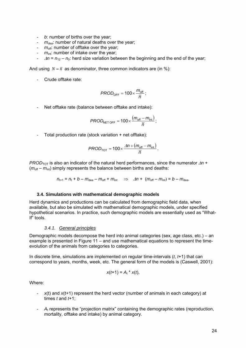
3.4. Simulations with mathematical demographic models Herd dynamics and productions can be calculated from demographic field data, when available, but also be simulated with mathematical demographic models, under specified hypothetical scenarios. In practice, such demographic models are essentially used as “What-If” tools.

3.4.1. General principles

Demographic models decompose the herd into animal categories (sex, age class, etc.) – an example is presented in Figure 11 – and use mathematical equations to represent the time-evolution of the animals from categories to categories. In discrete time, simulations are implemented on regular time-intervals (t, t+1) that can correspond to years, months, week, etc. The general form of the models is (Caswell, 2001):

x(t+1) = At * x(t), Where:

- x(t) and x(t+1) represent the herd vector (number of animals in each category) at times t and t+1;

- At represents the “projection matrix” containing the demographic rates (reproduction,

mortality, offtake and intake) by animal category.

24

In annual models, herd dynamics are calculated from years to years by the following equations:

x(1) = A0 * x(0), x(2) = A1 * x(1) = A1 * A0 * x(0), x(3) = A2 * x(2) = A2 * A1 * A0 * x(0), etc. (Where x(0) represents the initial herd vector).

The required input data of these models are the:

- Initial herd size by animal category (e.g. sex and age classes like female and male juveniles/sub-adults/adults);

- Annual demographic rates by animal category.

When possible, these data can be calculated from field surveys or in experimental farms. Nevertheless, in practice they are frequently set from guess estimates or literature reviews (e.g. scientific journals or non published reports).

3.4.2. Variable versus constant demographic environment

Demographic rates values in the projection matrix At summarize the effect of a large number of factors: climate, feed resources, genetics, farming practices, etc. In livestock demography, all these factors are considered as the “environment” of the herd.

(a) Variable environment In annual demographic models, the environment is said variable when the annual projection matrix varies from years to years, i.e. when x(t+1) = At * x(t). For instance, one matrix can be defined for a year with goods rains, versus another matrix for a year of drought. The time-sequences of matrices At can be modelled following different variability patterns, for instance randomly or in relation to external variables (climate, market access, etc.).

(b) Constant environment The environment is said constant when the annual projection matrix does not vary, i.e. when x(t+1) = A * x(t). The previous dynamics equations x(t+1) = At * x(t) become:

x(1) = A * x(0), x(2) = A * x(1) = A2 * x(0 x(3) = A2 * x(2) = A3 * x(0),

etc.

25

In that constant environment, herd dynamics starts by showing growth rate fluctuations and then, after a given period (referred to as “transient regime”), converge to a status named “steady state” (Caswell, 2001). This steady state is characterized by a:

- Stable sex-by-age structure (proportions of all animal categories remain constant with time);

- Stable annual growth rate

The steady state depends only on the demographic rates in matrix A, and not on the initial herd structure x(0). It can be calculated directly from A, without using the dynamics equations and running the model for a long time. Only one “average” year is simulated.

3.4.3. Practical applications

Models representing variable environments are well adapted to simulate long term herd dynamics (e.g. for period of 20 years or more), for instance to represent the impacts of shocks (mortalities/destocking due to outbreaks, droughts, etc.) or the expected results of herd restocking programs. Steady state models are better adapted to simulate the mean herd dynamics (stable annual growth rate and herd structure) and productions under different scenarios assuming an almost constant environment, as well as the potential impact of innovations. They also can help to assess the validity of estimations of global production indicators (e.g. PRODTOT) estimated from data routinely collected in the field. An example of MS Excel interface (DYNMOD) available to implement a simple demographic model (with modules representing variable or constant environments) is presented in the Annexes section.

26

Births

Females

Juveniles

Sub-adults

Adults

Final culling

Natural death(pdeath, F, J)

Offtake(pofftake, F, J or/and surplus)

Intake(nF, J)

γF, J * sF, J

Natural death(pdeath, F, S)

Offtake(pofftake, F, J or/and surplus)

Natural death(pdeath, F, S)

Offtake(pofftake, F, S or/and surplus)

γF, S * sF, S

γF, S * sF, S

Births

Males

Juveniles

Sub-adults

Adults

Final culling

Natural death(pdeath, M, J)

Offtake(pofftake, M, J or/and surplus)

γM, J * sM, J

Natural death(pdeath, M, S)

Offtake(pofftake, M, J or/and surplus)

Natural death(pdeath, M, S)

Offtake(pofftake, M, S or/and surplus)

γM, S * sM, S

γF, M * sF, M

pbirth, F 1 - pbirth, F

f

Intake(nF, S)

Intake(nF, A)

Intake(nM, J)

Intake(nM, S)

Intake(nM, A)

Figure 11: Example of animal life cycle defining the structure of a simple demographic model (source: MS Excel interface DYNMOD freely available at the following address: ftp://ftp.cirad.fr/cirad/livtools/Materials/DYNMOD/).

27

4. Recommendations

4.1. Introduction The consultancy recommends the following methodological framework, split into two parts concerning:

- The field data collection enabling the calculation of demographic parameters in a given DT/CP ruminant livestock population, considered as the “target” population ;

- The calculation of the demographic parameters derived from these data.

The DT/ CP model used is as follows: A DT/CP catchment area (“zonal”) is composed of several farms (herds) which are regularly surveyed using the dip tank or the crush pen facility (e.g. on a biweekly, or monthly or yearly basis). The observation unit remains the farm which is surveyed when the related herd is using the DT/ CP. The simplified methodological framework presented here is described for one given species (e.g. cattle, sheep or goats) and is based on the following principles and assumptions:

- Data are firstly collected representing the farm (herd), then data are aggregated to the DT/CP level (several farms);

o Aggregation of data to higher levels than DT/CP (e.g. aggregation of several DT/CP data in a district or a country) follows the same principle but is not detailed in this report.

- Data collection is exhaustive, i.e. all farmers (herds owners) present in the DT/CP

area at the time of the survey are interviewed; o Nevertheless, an additional recommendation is provided in a forthcoming sub-

section of this Chapter to adapt the proposed framework when only a sample of the herds of the DT/CP is sampled;

- Data are collected with two alternative frequencies: once a month (e.g. during a

monthly intervention) or annually (e.g. during annual vaccinations); o any other frequency can be used to reflect any intervention pace, e.g. a

weekly dipping - Data are collected with two alternative levels of details for describing the herd and the

demographic events: o Global collection for the whole herd without differentiating animal categories

(e.g. all cattle); o Collection by animal category (e.g. by sex and age class of cattle);

- At each date of survey, the collected data are:

o The herd size (global or by animal category) at date of survey; o The number of demographic events (per type of event, global or by animal

category) occurred in the herd, during the last month in case of monthly surveys, or during the last year in case of annual surveys.

The frequency of data collection and the level of globalization versus categorization of animals as implemented in practice by countries, depend on the level of details required and on the available human and financial resources available.

28

4.2. Data collection at herd level

4.2.1. Data collection without animal categorization

For each date of survey, data to be collected in the herd are the:

- Herd size; - Number of demographic events occurred in the herd during the retrospective period

considered in the framework (month or year): o Reproductions; o Exits from the herd; o Entries in the herd.

Several levels of details can be defined for describing demographic events when collecting the data:

- The minimum recommended level is presented in Table 3; - Table 4 presents a more detailed level:

o It uses finest decompositions of the types of demographic events; o It specifies the destination/origin of the exits/entries, transfer in or transfer out

of the DT/CP area. In the aggregated model, “Transfer in” animals still belong to the area, whereas “transfer out” animals exit the area.

All intermediated levels between Table 3 and Table 4 levels could also be considered. In the forthcoming text, the report assumes that Table 3 level has been chosen as a reference. The principle of the procedures presented is exactly the same when other levels of details (e.g. Table 4) are considered.

4.2.2. Data collection with animal categories

In this case, the same table as Table 3 has to be built and filled in for each animal category. The generated table has two dimensions. For instance, the rows of the table can represent the variables of Table 3 and the columns the animal categories. Categories should describe the sex (females/males) and the age class of the animals (e.g., juveniles/sub-adults/adults). For cattle, common categories are as follows:

- Female calves, Heifers (un-mature females), Cows (mature females); - Male calves, Steers (un-mature male), Bull, Oxen.

For small ruminants, common categories are as follows:

- Females: 0 to 1 year, >1 year; - Males: 0 to 1 year, >1 year.

In any case, definitions of the animal categories have to be consistent over time and across the country.

29

Table 3: Variables to be collected at farm level at each survey (minimum level of detail).

Variable collected

Notation Description

State variable N Total herd size at date of survey - Number of animals

Events Number of events during the retrospective period (past month or year):

PAR Parturitions - Only deliveries at term (exclude abortions)

Reproduction

B Births - Only born alive (exclude stillborn)

DEA Natural deaths - Predations - Other causes (diseases, malnutrition, old age, etc.)

SLA Slaughtering at farm - Self-consumption

SAL Sales - To:

o Farms (direct, auction, etc.) o Traders o Abattoirs

- To In or out the DT area GIFEXI Permanent gifts

- To In or out the DT area LOAEXI Temporary loans(a)

- To In or out the DT area THEEXI Thefts

Exits

DIS Disappearances - Disappearing with unknown cause

PUR Purchases (from in or out the DT area) - From:

o Farms (direct, auction, etc.) o Traders o Abattoirs

- From In or out the DT area GIFENT Permanent gifts

- From In or out the DT area LOAENT Temporary loans(b)

- From In or out the DT area

Entries

THEENT Recovering from thefts - Source: police

(a) Loans exits can be of two types: the farm owns an animal and lends it to another farm or the farm sends back a loaned animal to the owner. (b) Loans entries can be of two types: the farm receives an animal of another farm (owning the animal) or the farm receives back an animal it owns, from another farm (in which the animal was lent).

30

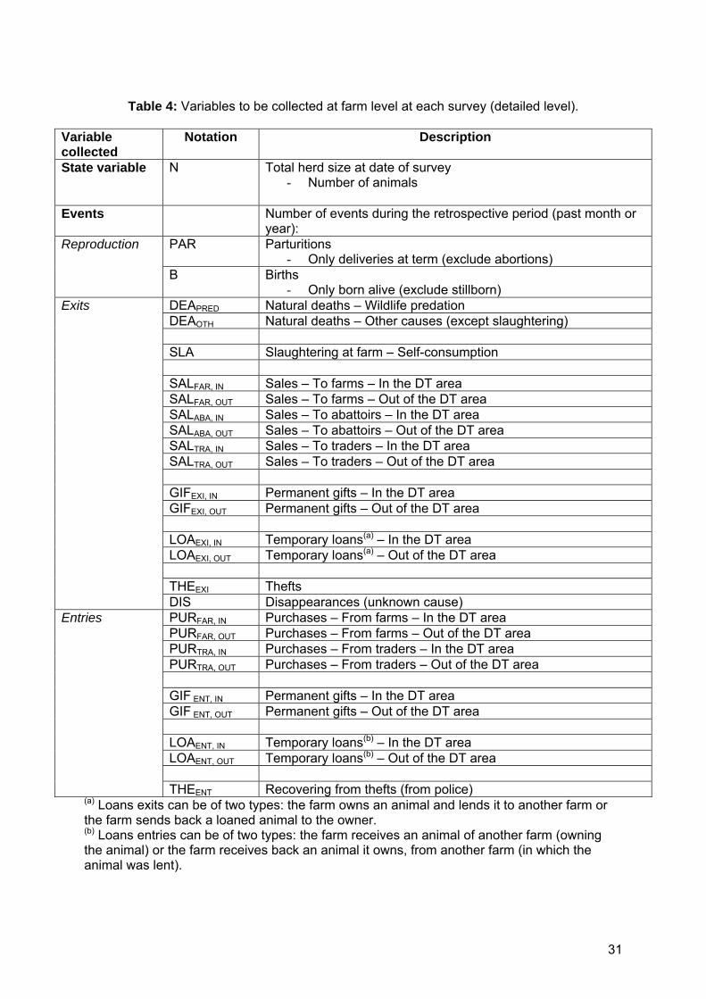
Table 4: Variables to be collected at farm level at each survey (detailed level).

Variable collected

Notation Description

State variable N Total herd size at date of survey - Number of animals

Events Number of events during the retrospective period (past month or year):

PAR Parturitions - Only deliveries at term (exclude abortions)

Reproduction

B Births - Only born alive (exclude stillborn)

DEAPRED Natural deaths – Wildlife predation DEAOTH Natural deaths – Other causes (except slaughtering) SLA Slaughtering at farm – Self-consumption SALFAR, IN Sales – To farms – In the DT area SALFAR, OUT Sales – To farms – Out of the DT area SALABA, IN Sales – To abattoirs – In the DT area SALABA, OUT Sales – To abattoirs – Out of the DT area SALTRA, IN Sales – To traders – In the DT area SALTRA, OUT Sales – To traders – Out of the DT area GIFEXI, IN Permanent gifts – In the DT area GIFEXI, OUT Permanent gifts – Out of the DT area LOAEXI, IN Temporary loans(a) – In the DT area LOAEXI, OUT Temporary loans(a) – Out of the DT area THEEXI Thefts

Exits

DIS Disappearances (unknown cause) PURFAR, IN Purchases – From farms – In the DT area PURFAR, OUT Purchases – From farms – Out of the DT area PURTRA, IN Purchases – From traders – In the DT area PURTRA, OUT Purchases – From traders – Out of the DT area GIF ENT, IN Permanent gifts – In the DT area GIF ENT, OUT Permanent gifts – Out of the DT area LOAENT, IN Temporary loans(b) – In the DT area LOAENT, OUT Temporary loans(b) – Out of the DT area

Entries

THEENT Recovering from thefts (from police) (a) Loans exits can be of two types: the farm owns an animal and lends it to another farm or the farm sends back a loaned animal to the owner. (b) Loans entries can be of two types: the farm receives an animal of another farm (owning the animal) or the farm receives back an animal it owns, from another farm (in which the animal was lent).

31

4.3. Data aggregation at the DT/CP level (spatial aggregation) For each date of survey, data collected at farm level have to be aggregated at the DT/CP level. Two situations are possible. In both situations, the aggregation generates a DT/CP table with the same structure as Table 3.

4.3.1. Situation where the herds of the DT/CP area are surveyed exhaustively

In this situation, for each date of survey, variables collected at farm level in Table 3 simply need to be summed up over all the herds.

4.3.2. Situation where only a sample of herds is surveyed

In this situation, the aggregation needs to be done in two steps:

- Step1: As in the exhaustive situation, variables collected at farm level in Table 3 have to be summed over the surveyed herds. As before, this generates a DT/CP table with the same structure as Table 3;

- Step 2: Then, the generated table (representing the herds’ sample) has to be

corrected to represent the whole DT/CP livestock population. Assuming that K is the total number of herds in the DT/CP area and k the number of surveyed herds (the sample), all data aggregated in Step 1 have to be multiplied by K/k.

4.4. Data aggregation over the year (temporal aggregation) After aggregation at the DT/CP level for each date of survey, the generated DT/CP-level data have to be aggregated over the year, for preparing the calculations of the annual demographic parameters. The objective of this aggregation is to get:

- The mean herd size (or the mean size of the animal category, if data are collected by category) over the year. This mean size will be used as denominator in the calculation of the demographic and production rates3;

- The total numbers of demographic events (by animal category, if data are collected

by category) occurred during the year, per type of events described in Table 3. These numbers will be used as numerators in the calculation of the demographic and production rates.

The aggregation process depends on the surveys frequency (monthly or annually for the purpose of the demonstration).

4.4.1. Case of monthly surveys

Considering a given year y, with the same notations as in Figure 10, the mean herd size over year y can be calculated by:

3 Or epidemiological rates

32

1312

0∑

=

=t

tNn .

For each date of survey t, the demographic events data consist in the numbers of events occurred in the past month. Data to be aggregated for year y correspond to t= 1, 2, …, 12. Date t=0 has to be removed since it concerns month 12 of year y-1. For instance, the annual number of natural deaths in year y should be calculated by:

∑=

=12

1iiDEADEA .

Other events of (parturitions, births, slaughtering, etc.) can be calculated with the same principle.

4.4.2. Case of annual surveys

Considering a given year y, with annual surveys at dates t=0, 13 (using same notations as for monthly surveys), the mean herd size over year y can be calculated by:

( ) 2130 NNn += . In case of annual surveys, collected data are retrospective annual data. Therefore, the demographic events data for year y correspond to data collected at date of survey t=13 and no aggregation over time is needed.

4.5. Demographic calculations

4.5.1. Preliminaries

Consider the general dynamics equation presented in the theoretical background chapter:

nt+1 = nt + b – mdea – moff + mint ⇒ ∆n + (moff – mint) = b – mdea. Using variables described in Table 3 and for year y, this equation can be translated by:

N13 = N0 + B – DEA – SLA – SAL – GIFEXI – LOAEXI – THEEXI – DIS + PUR + GIFENT + LOAENT + THEENT.

In demography, definitions of what represent the “offtake”, “intake”, “net offtake”, “losses”, etc. depends on the objectives of the data analyses. In the forthcoming text, the definitions are as follows:

- Offtake groups slaughtering, sales, permanent gifts and loans:

OFF = SLA + SAL + GIFEXI + LOAEXI; - Intake groups purchases, permanent gifts and loans:

INT = PUR + GIFENT + LOAENT;

33

- Losses (other than natural deaths) groups net thefts and withdrawals:

LOS = THEEXI – THEENT – DIS. The corresponding dynamics equation becomes:

N13 = N0 + B – (DEA + LOS) – OFF + INT ⇒ ∆N + (OFF – INT) = B – (DEA + LOS). The term (DEA + LOS) represents the “global losses” for the livestock population.

4.5.2. Basic demographic parameters

The basic demographic parameters can be calculated for the whole population or by animal category (sex, age class).

(a) Reproduction

- Parturition rate: n

mh par

par 100 ×= ;

- Net fecundity rate: n

mh birfec net 100 ×= ;

- Net prolificacy rate: prolnet = mbir / mpar; Where: mpar = PAR, mbir = B. Both rates hpar and hbir are poorly informative when they are calculated over the whole herd. More pertinent rates are obtained by dividing PAR and B by the mean number of adult females (= females assumed as mature).

(b) Other basic rates

- Mortality rate: n

mh deadea 100 ×= ;

- Loss rate: n

mh loslos 100 ×= ;

- Offtake rate: n

mh offoff 100 ×= ;

- Intake rate: n

mh intint 100 ×= ;

Where: mdea = DEA, mlos = LOS, moff = OFF, mint = INT.

4.5.3.

34

Global demographic indicators

The global demographic indicators are generally calculated for the whole population, without considering animal categories.

(a) Dynamics

- Annual population growth rate (in %): ⎟⎟⎠

⎞⎜⎜⎝

⎛−×= 1100

0

13

NNAGR .

(b) Production

- Crude offtake rate (in %): n

mPROD offOFF 100 ×= ;

- Net offtake rate (in %): ( )n

mmPROD intoffOFF NET 100 −

×= ;

- Total production rate (in %): ( )n

mmnPROD intoffTOT 100 −+

×=∆ ;

Where: moff = OFF, mint = INT, ∆n = ∆N.

4.6. Training on Livestock demographic methods The consultancy recommends a standard training session on livestock population demographic modelling be with the following features. Duration: 3 days Possible curriculum:

- Day1: Presentation of concepts on demographic models; - Day2: Case studies & exercises (in working groups) with the use of DYNMOD:

Reasons why using demographic modelling, the questions posed? Review of data usable in countries (sources, quality), selection of appropriate scenarios, running models, presenting results in reports;

- Day3: Presentation of the case study results from modelling exercises, debriefing and

discussion, ways of improvements

35

5. References cited in the report Agresti, A., 1990. Categorical data analysis. Wiley. Aitkin, M., Anderson, D., Francis, B., Hinde, J., 1989. Statistical modelling in GLIM. Clarendon Press Oxford. Anderson, D.R., Burnham, K.P., 1976. Population of the Mallard. VI. The effect of exploitation on survival. Ressource Publication 128. United States Department of the Interior Fish and Wildlife Service Washington D.C., USA. Caswell, H., 2001. Matrix population models: construction, analysis and interpretation. Sinauer Associates Sunderland. Chiang, C.L., 1984. The life table and its application. Robert E. Krieger Publishing Company Malabar, Florida. Collett, D., 2003a. Modelling binary data. Chapman & Hall/CRC New York. Collett, D., 2003b. Modelling survival data in medical research. Chapman & Hall/CRC New York. Cox, D.R., Oakes, D., 1984. Analysis of survival data. Chapman and Hall New York. Kalbfleisch, J.D., Prentice, R.L., 1980. The statistical analysis of failure time data. Wiley New York, USA. Laird, N., Olivier, D., 1981. Covariance analysis of censored survival data using log-linear analysis techniques. J.A.S.A 76, 231-240. Larson, M.G., 1984. Covariate analysis of competing risks data with log-linear models. Biometrics 40, 459-469. Lee, E.T., 1992. Statistical methods for survival data analysis. Wiley New York, USA. Lesnoff, M., Lancelot, R., Moulin, C.H., 2007. Calcul des taux démographiques dans les cheptels de ruminants domestiques tropicaux: approche en temps discret. CIRAD (Centre de coopération internationale de recherche agronomique pour le développement), ILRI (International livestock research institute). Editions Quae.http://www.quae.com/numerique. Lesnoff, M., Messad, S., Juanès, X., 2009. 12MO: A cross-sectional retrospective method for estimating livestock demographic parameters in tropical small-holder farming systems. CIRAD (French Agricultural Research Centre for International Development) Montpellier, France. McCullagh, P., Nelder, R.W.M., 1989. Generalized linear models. Chapman and Hall New York.

36

6. Annexes

6.1. Probabilities and hazard rates in demography A number of basic concepts relating to rates in demography are presented below. Calculation of rates relating to tropical domestic populations is discussed in Lesnoff (2000) and Lesnoff et al. (2007). Readers are also referred to the many publications on survival analysis methods (e.g. Anderson and Burnham, 1976; Kalbfleisch and Prentice, 1980; Chiang, 1984; Cox and Oakes, 1984; Lee, 1992; Collett, 2003b). In the area of demography, rate of occurrence of an event may represent two distinct mathematical parameters: a probability and an instantaneous hazard rate, which in this report are notated p and h, respectively. This can give rise to ambiguities when definition of rates and calculation methods are not described in detail. Several terms have been used for h – hazard function, instantaneous hazard rate or intensity of risk. The below description of these parameters derives from Collet (2003b), taking the example of mortality. The instantaneous hazard rate for mortality hdeath(t) is the risk of natural death per unit of time, at time t: the quantity hdeath(t)dt is the expected proportion of surviving animals at time t that will die within the small interval (t, t + dt). More formally, consider the random variable T that represents the lifetime of an animal. In absence of any other cause of removal apart from death, probability that an animal surviving at time t will die within the time interval (t, t + dt) is P(t ≤ T < t+dt | T ≥ t), where “|” is the conditional operator. To obtain a rate per unit of time, this conditional probability is divided by the length of the time interval dt. The instantaneous hazard rate is the limit of this value when dt tends towards 0:

( ) ( ) .dt

tdtTtTtPlimth dt≥+<≤

= →0death

In the area of livestock-raising, instantaneous offtake rate hofftake(t), is defined in the same way as hdeath(t). Total instantaneous hazard rate of removal is htotal(t) = hdeath(t) + hofftake(t). A probability ranges from 0 to 1 and has no unit, whereas an instantaneous hazard rate can be greater than 1 and is expressed per unit time. Under some circumstances, the two parameters are connected by functional relationships (in which case p can be estimated on the basis of h and vice-versa). For instance, if one assumes that the only cause of removal is natural death and that the instantaneous hazard rate hdeath is constant for the period (t, t+∆t), probability of natural death pdeath during that period can be calculated using the formula (Kalbfleisch and Prentice, 1980; Chiang, 1984; Cox and Oakes, 1984; Lee, 1992):

pdeath = 1 – exp(–hdeath ∆t). Hence, an instantaneous hazard rate for death of 0.50/year (= 0.0417/month) is associated with an annual probability of dying of 0.39 (with no offtake), which means that 39%, not 50%, of the animals will die on average in a year. When there are other causes of removal (e.g., offtake), which are referred to as competing risks, probability of death decreases and becomes an “apparent” probability of death (this is due to the fact that animals removed as offtake will “escape” to the daily natural death risk, which here is hdeath/365). It can be computed as follows (Anderson and Burnham, 1976; Chiang, 1984):

37

( )( )[ ]

( ).thexp

,thhexphh

hp

∆

∆

death

offtakedeathofftakedeath

deathdeath

1

1

−≤

+−−+

=

For example, death rate hdeath = 0.50/year corresponds to an annual death probability pdeath = 0.39 when there is no offtake (hofftake = 0), and to pdeath = 0.33 when hofftake = 0.40/year. In the first case, 39% of the animals will die in average over the year and, in the second case, only 33%. When data are grouped by category of animal and by period, probability of occurrence p and instantaneous hazard rate h can be estimated respectively by:

p = m / n and h = m / T, where m is the number of events (of a given type) that occurred in the period, n the number of animals present at the beginning of the period and T the total time of presence of these animals during the period, which in epidemiology is called the time at risk. Statistical methods for analysing parameters p and h, and more generally for count data, are numerous and have been widely described. One of the more common methods is the generalized linear models, such as logistic regression for probabilities and log-linear regression for instantaneous hazard rates (Laird and Olivier, 1981; Larson, 1984; Aitkin et al., 1989; McCullagh and Nelder, 1989; Agresti, 1990; Collett, 2003a).

6.2. DYNMOD – A simple MS Excel interface for simulating ruminant livestock demography

6.2.1. Background

Tools for evaluating the impact of development projects or shocks (like drought or outbreaks) on the livestock dynamics and production are helpful to better target strategies for improving economic situation of livestock smallholders. In that context, CIRAD (French Agricultural Research Centre for International Development) and ILRI (International Livestock Research Institute) have recently developed DYNMOD, a simple tool for simulating demography of tropical ruminant livestock populations. DYNMOD was developed under Microsoft® Office Excel 2003. The tool is intended for operational or educational uses. It can be used by researchers, engineers and technicians of national services, development professionals or students dealing with demography of tropical ruminant livestock (cattle, small ruminants and camels), in various fields such as animal science, genetics, epidemiology, or economy. All DYNMOD materials (manual, Excel files and examples) can be freely downloaded at the FTP address ftp://ftp.cirad.fr/cirad/livtools/Materials/DYNMOD/.

6.2.2. General characteristics

DYNMOD is well adapted for fast and crude ex ante or ex post diagnostics, in various applications as for example livestock population management, herd production estimation or exploration of scenarios in development projects. Based on simplified deterministic demographic processes, DYNMOD simulates the dynamics of the population size and the number of animals produced per year. DYNMOD also

38

calculates live weights, meat production and secondary productions (milk, skin and hides, manure) at population level, as well financial outputs that can be used in more integrated financial calculations (e.g. benefit-costs ratios or internal return rates). Finally, DYNMOD provides crude estimates of the population feeding requirements in dry mater. DYNMOD predicts what would happen under some hypothetical scenarios, not what will happen in the real world. In that sense, DYNMOD is more a projection model than a prediction model (Caswell, 2001). In a simulation, the user has to judge by itself of the relevancy of the scenario considered. The actual version of DYNMOD consists in three modules, based on the same underlying demographic model (Figure 11) but representing different hypotheses:

- STEADY1: simulation of the 1-year population production assuming a demographic steady state – with constant sex-by-age structure and annual growth rate;

- STEADY2: simulation of the 1-year population production assuming a demographic

steady state – with constant adult population size and null growth rate. STEADY2 is a particular case of STEADY1;

- PROJ: simulation of the population dynamics and production of a over a period of

time in a possibly variable environment (the period can last from 1 to 20 years). The consultancy recommends the user to refer to the DYNMOD handbook (ftp://ftp.cirad.fr/cirad/livtools/Materials/DYNMOD/), which details the demographic mathematical equations and the parameters used in the model and describes different simple case-studies.

39

6.3. Manual DYNMOD Version 6 The manual is freely downloadable at the following FTP address: ftp://ftp.cirad.fr/cirad/livtools/Materials/DYNMOD/) The link will be available under the LIMS web portal (http://aims.sadc.int livestock section) in the demographic study section of PRINT-LIMS pages.

40