Embed Size (px)
Citation preview

SAFETY EFFECTS OF MULTIMODAL INFRASTRUCTURE
AND ACCESSIBILITY IN URBAN TRANSPORTATION
SYSTEMS
by
Ivana Tasic
A dissertation submitted to the faculty of The University of Utah
in partial fulfillment of the requirements for the degree of
Doctor of Philosophy
Department of Civil and Environmental Engineering
The University o f Utah
August 2016

Copyright © Ivana Tasic 2016
All Rights Reserved

The U n i v e r s i t y o f Ut ah G r a d u a t e S c h o o l
STATEMENT OF THESIS APPROVAL
The thesis o f Ivana Tasic_________________________________________________________
has been approved by the following supervisory committee members:
________________ Richard J. Porter_________________ , Chair 02/29/2016Date Approved
________________Xiaoyue Cathy Liu________________ , Member 02/29/2016Date Approved
_________________ Milan Zlatkovic__________________ , Member 02/29/2016Date Approved
_________________ Daniel Fagnant__________________ , Member 02/29/2016Date Approved
___________________ Reid Ewing____________________ , Member 02/29/2016Date Approved
and by _________________________Michael Barber_________________________ , Chair of
the Department o f Civil and Environmental Engineering
and by David B. Kieda, Dean o f The Graduate School.
ABSTRACT
The interest in multimodal transportation improvements is increasing in cities across
the U.S. Investing in multimodal infrastructure benefits the portion of urban population
that is unable to drive due to a variety of reasons such as personal preference, age, and
affordability. It is also well known that active transportation such as walking, biking, and
taking transit, can improve public health due to increased physical activity, and reduce
traffic congestion by reducing the average person’s delay. While improved multimodal
infrastructure and accessibility attracts new users, it can possibly increase their exposure
to risk from crashes. In urban areas where the “safety in numbers phenomenon” does not
exist, nonmotorized user vulnerability becomes a predominant risk factor when they are
involved in a crash, even at lower vehicle speeds.
This dissertation aims to explore the factors that are associated with safety outcomes
in urban multimodal transportation systems, and develop methods that can be used to
estimate safety effects of multimodal infrastructure and accessibility improvements.
Using Chicago as a case study, a comprehensive dataset is developed that significantly
contributes to the existing literature by including socio-economic, land use, road network,
travel demand, and crash data. Area-wide analysis on the census tract level provides a
broader perspective about safety issues that multimodal users encounter in cities. The
characteristics of a multimodal transportation system are expressed through the presence
of multimodal infrastructure, street connectivity and network completeness, and

accessibility to destinations for multimodal users. A set of statistical areal safety models
(SASM) based on both frequentist and Bayesian statistical inference is applied to
estimate the factors that are associated with total and severe vehicular, pedestrian, and
bicyclist crashes in urban multimodal transportation systems.
The results show that the current safety evaluation methods need to acknowledge the
complexity of multimodal transportation systems through the inclusion of diverse factors
that may influence safety outcomes, particularly for more vulnerable users. The methods
developed in this research can further be used to expand the current practice of evaluating
multimodal transportation safety, and planning for city-wide investments in multimodal
infrastructure and improved accessibility, while being able to estimate the expected safety
outcomes.
iv
ABSTRACT.................................................................................................................................iii
LIST OF TABLES.....................................................................................................................vii
LIST OF FIGURES................................................................................................................... ix
ACRONYMS.............................................................................................................................. xi
ACKNOWLEDGEMENTS.................................................................................................... xiii
Chapter Page
1 INTRODUCTION.....................................................................................................................1
Research Problem Statement................................................................................................... 3Research Objectives................................................................................................................. 4Conceptual Framework............................................................................................................7Dissertation Outline.................................................................................................................. 8
2 LITERATURE REVIEW ...................................................................................................... 10
Multimodal Transportation Safety....................................................................................... 10Areal Safety Studies............................................................................................................... 12The Role of Exposure and Surrogate M easures................................................................. 14Measures of Multimodal Accessibility................................................................................18Other Relevant Variables in Areal Safety Studies.............................................................29Crash Analysis Methods in Areal Safety Studies............................................................... 29Summary of Literature...........................................................................................................31
3 METHODOLOGY................................................................................................................. 34
Research Design......................................................................................................................35Data Collection........................................................................................................................36Response Variables................................................................................................................ 42Measures of Exposure............................................................................................................46Measures of Multimodal Accessibility................................................................................50Explanatory Variables Representing System-wide Effects...............................................79Statistical Areal Safety Modeling M ethods........................................................................85
TABLE OF CONTENTS

Preliminary and Final Model Specifications.....................................................................106Diagnostics and Final Model Recommendations.............................................................107
4 STATISTICAL AREAL SAFETY MODELING RESULTS........................................ 111
Preliminary Model Specifications...................................................................................... 112Final Model Specifications.................................................................................................. 113Diagnostics and Final Model Recommendations.............................................................121Safety Effects of Multimodal Exposure and Accessibility.............................................121
5 DISCUSSION OF STATISTICAL AREAL SAFETY MODELING RESU LTS...... 134
Preliminary Model Specifications...................................................................................... 134Final Model Specifications.................................................................................................. 135Diagnostics and Final Model Recommendations.............................................................152Safety Effects of Multimodal Exposure and Accessibility.............................................156
6 CONCLUSIONS AND RECOMMENDATIONS...........................................................161
Research Contributions........................................................................................................161Research Limitations............................................................................................................167Future Research N eeds.........................................................................................................168
REFERENCES......................................................................................................................... 171
vi

Table Page
1. Data Sources, Descriptions, and Form ats.......................................................................... 38
2. Descriptive Statistics for Road Crashes............................................................................. 43
3. Descriptive Statistics for the Road Network, Traffic, and Multimodal Transportation Variables.................................................................................................................................49
4. Descriptive Statistics for Network Completeness............................................................. 53
5. Descriptive Statistics for Variables Capturing Destination Accessibility.....................71
6. Descriptive Statistics for the SE Variables........................................................................82
7. Descriptive Statistics for Land Use Variables.................................................................. 84
8. Preliminary Specification of NB Model Used to Obtain Final Model Specifications for Total Vehicular, Pedestrian, and Bicyclist Crashes...................................................... 112
9. Preliminary Specification of NB Model Used to Obtain Final Model Specifications for Vehicular, Pedestrian, and Bicyclist Severe Crashes.................................................... 113
10. Total Vehicular Crash M odels........................................................................................ 114
11. Severe Vehicular Crash Models...................................................................................... 115
12. Total Pedestrian Crash M odels....................................................................................... 116
13. Severe Pedestrian Crash Models.....................................................................................117
14. Total Bicycle Crash Models.............................................................................................118
15. Severe Bicycle Crash M odels......................................................................................... 119
16. Diagnostics for NB, FENB, RENB, GAM, and FBH Models....................................124
17. Recommended Model for Total Vehicle-only Crash Estimation.............................. 124
LIST OF TABLES

18. Recommended Model for Vehicle-only KA Crash Estimation..................................124
19. Recommended Model for Total Pedestrian Crash Estimation....................................125
20. Recommended Model for Pedestrian KA Crash Estim ation...................................... 125
21. Recommended Model for Total Bicyclist Crash Estimation...................................... 126
22. Recommended Model for Bicyclist KA Crash Estimation......................................... 126
viii

LIST OF FIGURES
Figure Page
1. Conceptual Framework...........................................................................................................8
2. Spatial Units of Analysis Considered in This Study with the Description of Census Tract Area as the Selected Unit of Analysis......................................................................41
3. Spatial Distribution of Crashes by Census Tract in Chicago for Time Period from 2005 to 2012....................................................................................................................................44
4. Normal Q-Q Plot, Histograms, and Box Plots for Vehicle-only, Pedestrian, and Bicyclist Total and Severe (KA) Crashes, Respectively.................................................45
5. Roadway Network and Multimodal Facilities.................................................................. 53
6. Spatial Distribution of DVMT and the Percentage of the City of Chicago Street Network Serving All Four M odes...................................................................................... 54
7. Destinations Accessible Within the Given Walking Tim e..............................................61
8. Destinations Accessible Within the Given Biking Tim e.................................................64
9. Daily Changes in Transit Stop Frequency by Station on the Census Tract Level....... 72
10. Number and Percentage of Transit Stops Accessible Within the Given Amount of Time Budget......................................................................................................................... 74
11. Daily Variations of Transit Accessibility for All Census Tracts Dependent on Preferred Walk Time Within the 60-minute Available Time Budget.......................... 75
12. Daily Variations of Transit Accessibility for All Census Tracts Dependent on the Available Budget Time Within the 5-minute Walk from the Transit Stations...........76
13. Incremental Change in Transit Accessibility Depending on the Available Time Budget and Walking D istance.......................................................................................... 77
14. Destinations Accessible Within the Given Travel Time by Transit............................ 78

15. Spatial Distribution of the Population Density and the Percent Unemployed Population in Chicago (U.S. Census ACS 5-Year Data, 2008 - 2012)........................ 81
16. Land Use Parcels and Land Use Entropy in Chicago.................................................... 84
17. Flowchart of Crash Data Analysis Process......................................................................86
18. Monte Carlo Simulation of Moran’s I for Total Multimodal Crashes.........................93
19. Monte Carlo Simulation of Moran’s I for Severe (KA) Crashes..................................94
20. Local Moran’s I Results..................................................................................................... 96
21. Visualization of GAM for Some of the Statistically Significant Explanatory Variables in Total Crash Models...................................................................................................... 122
22. Visualization of GAM for Some of the Statistically Significant Explanatory Variables in Severe Crash M odels................................................................................................... 123
23. The “Safety in Numbers” Effect for Private Vehicle U sers....................................... 128
24. The “Safety in Numbers” Effect for Pedestrian Users.................................................129
25. Relationship Between Total Pedestrian Crashes and Accessibility Variables..........130
26. Relationship Between Severe Pedestrian Crashes and Accessibility Variables...... 131
27. The “Safety in Numbers” Effect for Bicyclist U sers................................................... 132
28. Relationship Between Bicyclist Crashes and Accessibility Variables......................133
x

ACRONYMS
SASM Statistical Areal Safety Modeling
GLM Generalized Linear Models
GAM Generalized Additive Models
FBH Full Bayes Hierarchical Models
SE Socio-Economic
DVMT Daily Vehicle Miles Traveled
HSM Highway Safety Manual
AASHTO American Association of State and Highway Transportation
Officials
TRB Transportation Research Board
MAUP Modifiable Areal Unit Problem
AADT Average Annual Daily Traffic
VMT Vehicle Miles Traveled
WMT Walk Miles Traveled
BMT Bike Miles Traveled
STP Space-Time Prism
AMELIA A Methodology Enhancing Life by Improving Accessibility
GIS Geographic Information System
DOT Department of Transportation

CMAP Chicago Metropolitan Agency of Planning
CTA Chicago Transit Authority
NHTS National Household Traveler Survey
ADT Average Daily Traffic
MUTCD Manual on Uniform Traffic Control Devices
FHWA Federal Highway Administration
OD Origin Destination
GTSF Google Transit Feed Specification
ACS American Community Survey
NB Negative Binomial
KA Severe (Fatal and Incapacitating Injury Crashes)
MCMC Monte Carlo Markov Chain
CAR Conditional Autoregressive Model
AIC Akaike Information Criterion
BIC Bayesian Information Criterion
DIC Deviance Information Criterion
CBD Central Business District
xii

ACKNOWLEDGEMENTS
My studies in the United States would not be possible without the support of my
family. I would like to wholeheartedly thank my Mom, Dad, and my Sister for their
unconditional love and encouragement over the past six years. I am forever grateful to all
my dear friends in Serbia who kept me in their lives regardless of the distance and time
we spent apart during my graduate school.
I am incredibly fortunate to have Dr. R.J. Porter as my advisor, as it was a privilege to
work with him and learn from him. His ability to be open for new ideas and his
dedication to high-quality research are what every doctoral student hopes to find in an
advisor.
I am thankful to my Doctoral Committee members for taking their time to provide
constructive comments about my research work over the past years. I sincerely thank all
the research project collaborators and sponsors, paper co-authors and contributors, and
faculty and staff members who shared their knowledge and experience to help me
complete my graduate studies. I am grateful for the support I always obtained from the
University of Utah Department of Civil and Environmental Engineering, the
opportunities to pursue multidisciplinary work on the University of Utah campus, and the
ground knowledge in transportation I obtained from the University of Belgrade School of
Traffic and Transport Engineering. Certainly this adventure would not have been nearly
as much fun without a long line of students-researchers from the Utah Traffic Lab, as

very few researchers get to work in such a diverse environment, and I am incredibly
grateful for having a chance to be a part of the team.
xiv
CHAPTER 1
INTRODUCTION
Transportation shapes the cities, which in return require transportation as the engine of
their economic, environmental, and social development. This interaction between cities
and their transportation systems is continuous, where the change of one always requires
further change of the other. Neglecting this relationship may lead to transportation
problems commonly faced by urban environments today, mostly resulting from urban
policies that favor one mode over the other modes of transportation (Jacobs, 1961;
Mumford, 1961; Vuchic, 1999).
Today, as the population living in the cities continues to increase, transportation and
mobility are central to sustainable urban development. The concept of “smart cities”
requires transportation system where “interaction is possible in any direction and at any
distance” and “streets are not an end in themselves.. .they are a means towards an end”
(Jacobs, 1961, p. 186; Lynch, 1960, p. 89). Over the course of several decades, these
concepts that tie cities and transportation together have slowly been transformed into
policies that prioritize the inclusion of all urban street users.
As cities across the U.S. increase their interest in multimodal transportation
investments and providing accessibility to multimodal options for all users, there is a
particular concern regarding the safety effects of these changes, particularly for more
vulnerable road users. The benefits of improving multimodal infrastructure and

accessibility range from better health outcomes through the use of active transportation
and reduced air pollution, to better mobility for those who cannot afford driving (United
Nations [UN] HABITAT, 2014). There is a general understanding that improved
multimodal transportation systems may lead towards resolving multiple long-term issues
related to sustainability and efficiency of travels in urban environments.
This movement towards more active and diverse transportation options in cities was
followed by the development of policy and guidelines for multimodal transportation, and
the need to extend existing evaluation methods to account for the presence of different
modes and their impacts on transportation performance. Improved access to multimodal
transportation attracts new users of alternative transportation modes, and safety of
multimodal users is still a topic that requires further research. Initiatives for creating more
sustainable transportation systems are gaining attention on the international scale, and the
need to reduce fatal road crashes remains in the focus of that effort. Safety emerges as a
global issue as the UN General Assembly declared the “UN Decade of Action for Road
Safety 2011-2020” supported by 100 world countries, as “nearly 1.3 million people are
killed on the world’s roads each year” (World Health Organization, 2010).
In cities across the U.S. that are developing or improving their multimodal
transportation features, the assessment of safety outcomes of improved multimodality is
still challenging. The methods of measuring the success and performance of multimodal
transportation systems are in the early stage of development, particularly in the area of
multimodal safety evaluations.
2

Research Problem Statement
In urban environments, where multimodal transportation thrives, the relationship
between access to multimodal transportation and safety is complex. Transportation
funding programs require that investments primarily focus on transportation performance,
including establishing quantitative transportation safety targets. With this need to
quantify safety outcomes, evaluation methods need to account for additional factors
associated with multimodal safety in urban environments.
As cities invest in multimodal infrastructure, accessibility for all users is improving,
which is a desirable outcome. However, with these improvements, the exposure of
multimodal users to conflicts with motorized users also increases, and the effects on
multimodal safety need to be examined. Transportation practitioners would benefit from
being able to estimate the expected safety effects of investments in multimodal
transportation and improving multimodal accessibility. In the short-term sense, this
knowledge would contribute to safety performance-based decision making, while the
long-term benefits would contribute to safety planning efforts and system-wide
improvements for multimodal users. The major impediments to gaining this knowledge
are the following existing limitations:
1) Data comprehensive enough to capture the complexity of multimodal
transportation systems in urban environments, while considering system-wide
effects as well as information on factors that potentially have a direct influence on
safety outcomes;
2) Measures that use the appropriate data to quantify the success of implemented
multimodal features in terms of their ability to provide access to opportunities for
3

all users as well as users’ activity and potential to be involved in conflicts that may
result in crashes;
3) Methods that draw from complex data and developed measures to estimate safety
effects for multimodal users, while dealing with the challenges which may arise in
extensive datasets, being flexible enough to be useful to both researchers and
practitioners, and enabling transferable application among different scales and
locations.
The opportunities to address these challenges for advancing knowledge on urban
multimodal safety are increasing with the emerging number of data sources on
multimodal users choices and activities, the paradigm shift in transportation performance
measurement towards more sustainable performance indicators, and the need to put the
emphasis on the safety of nonmotorized users as their vulnerability becomes a
predominant risk factor with the enhancement of multimodal transportation options.
Research Objectives
The goal of this research was to explore the factors that influence multimodal safety
outcomes in urban transportation systems, particularly focusing on the effects that
improved multimodal infrastructure and accessibility have on safety outcomes for
pedestrians, bicyclists, and private vehicle users. The defined research goal was
developed through three major objectives that align with the previously explained
research problem statement. These major research objectives were defined as the
following:
1) Develop a dataset consisting of spatially aggregated data to include multimodal
crash outcomes in urban environments, while capturing system-wide effects that
4
are associated with crashes according to the existing urban safety studies, as well
as detailed information about multimodal infrastructure;
2) Determine how multimodal users exposure can be represented, and develop
measures that may serve as the indicators of the level of success of multimodal
transportation system as well as the potential surrogate measures of exposure,
using the collected data;
3) Explore and apply a set of statistical areal safety modeling (SASM) methods that
will capture both system-wide effects and measures of multimodal presence in
urban environments, in order to estimate crash outcomes for pedestrians, bicyclists,
and private vehicle users.
Following these objectives, the City of Chicago was selected as the analysis location
due to its developed complete streets initiatives and extensive multimodal transportation
network features. A dataset was developed to allow for a system-wide analysis selecting a
census tract as the level of data aggregation. Aggregating the data in this way provided a
broader perspective about safety issues that multimodal users encounter in cities. The
system-wide effects captured in this manner include socio-economic features, land use
characteristics, road network, travel demand, and crashes. In this research, multimodal
safety outcomes are defined as 1) the expected number of total and severe vehicle-only
(vehicular crashes); 2) the expected number of total and severe crashes involving
pedestrians (pedestrian crashes); and 3) the expected number of total and severe crashes
involving bicyclists (bicyclist crashes). Severe crashes included fatal and severe injury
crashes for these three types of users.
5

Following the defined research objectives, several options were considered to
represent the exposure of multimodal users, as explained in the Methodology chapter. In
addition, measures that represent the level of access to multimodal transportation options,
including data on multimodal infrastructure and measures of multimodal connectivity and
accessibility, were developed to serve as proxies or surrogates for multimodal exposure.
The final part of the methodological approach in this research was using a set of
SASM methods to estimate vehicular, pedestrian, and bicyclist total and severe crashes as
a function of variables used to represent system-wide effects and measures of access to
multimodal transportation. The SASM methods were based on frequentist statistical
approach, including generalized linear (GLM) and generalized additive (GAM) models,
and Bayesian statistical approach used in Full Bayes Hierarchical (FBH) models. These
different SASM methods were used as a form of validation of the estimated crash
outcomes for multimodal users in urban environments.
This approach resulted in the ability to incorporate new variables that may influence
the safety of vulnerable transportation users into the SASM methods, explore different
SASM methods in terms of their ability to capture the system-wide effects and issues that
may arise in modeling spatially collected data, and use the estimated relationships and
provide recommendations for the development of safety evaluation methods for
multimodal users in urban environments. The research methodology was designed to
provide some insights to questions related to the variety of factors that may influence
urban safety in terms of both crash frequency and severity, the relationship between
access to multimodal transportation and safety, the methods that can be used to
successfully evaluate urban safety for different user and crash types, the expected number
6

7
of crashes under the given set of multimodal transportation features, and
recommendations about safety improvements in urban multimodal transportation
systems. The focus of this research was on the methodology, acknowledging that data
from other urban environments of various sizes should be collected in order to verify
transferability of findings from this study.
Conceptual Framework
Figure 1 presents the conceptual framework that serves as the core theoretical
hypothesis of this research that was used to develop the dataset, measures, and research
methodology. The core hypothesis is that areal units of analysis with different levels of
access to multimodal transportation, different levels of multimodal exposure, and
different system-wide characteristics are expected to have different multimodal crash
outcomes. Previous research on transportation mode choice addresses the relationship
between multimodal accessibility and exposure, influenced by system-wide effects such
as socio-economic (SE) features and land use patterns, leaving the statistical modeling of
this relationship beyond the scope of this research, but still acknowledged by the
conceptual framework. Key groups of variables and measures for each element of the
conceptual framework are also presented in Figure 1. Multimodal accessibility is
represented through the variables that should capture the physical presence of multimodal
infrastructure (e.g., bus lanes and stops, bike lanes, and bike racks), overall destinations
accessibility for a variety of modes, and network completeness in terms of the physical
street network share that serves multiple modes. Multimodal exposure is represented
through Daily Vehicle Miles Traveled (DVMT), trips generated by pedestrians and
bicyclists, commuter work trips by mode, and points of conflict between different modes.

8
Multimodal Accessibility _
f----------------------------\Multimodal Infrastructure
Street Connectivity
Network Completeness
Access to Destinations
________________________Challenge:
Multimodal accessibility analysis
System-wide Effects (Socio-Economic Data, Land Use)
Figure 1 Conceptual Framework
System-wide effects are provided through SE variables and land use characteristics.
Multimodal crash outcomes are represented as defined in the research objectives section
of this chapter. As previously stated, the conceptual framework served to develop the
methodological approach that estimates the expected number of total and severe
vehicular, pedestrian, and bicyclist crashes on the areal analysis level of census tract units
in the City of Chicago.
Dissertation Outline
This dissertation consists of six chapters. The first chapter introduces the research
problem, defines the research questions including the conceptual framework, and outlines
the proposed dissertation chapters. The second chapter presents the literature review
focused on urban multimodal transportation safety, areal safety studies, and the
representation of multimodal exposure and accessibility, summarizing the gaps in the
existing research and including the role that this research could play to fill in those gaps.
Multimodal Safety
/Total & Severe Vehicular
crashes
Total & Severe Pedestrian crashes
Total & Severe Bicyclist crashes
Challenge:
Estimation methods and crash data issues
Multimodal Exposure
Daily VMT
Trip generation by mode
Work trips by mode
Points of conflict
Challenge:
Adequate measures of exposure

The third chapter introduces the methodology, including data collection, variables,
measures, and SASM methods used to estimate the expected number of crashes for
multimodal users. Chapter 4 presents the results of the crash data analysis, starting from
preliminary model specifications to final “best models” by crash type. Chapter 5 is
focused on the interpretation of results presented in Chapter 4. Major contributions of this
research, recommendations for future research efforts, and research limitations are
provided in the final chapter.
9

CHAPTER 2
LITERATURE REVIEW
This chapter provides the review of previous research conducted in the area of urban
multimodal transportation safety. The chapter then continues to explain how areal safety
analysis is used to explore transportation safety for multimodal users, including the levels
of data aggregation, and the variety of effects captured in areal safety studies. Measures
of multimodal exposure and accessibility that exist in the literature are addressed,
including previous research on relationships between multimodal exposure, accessibility,
and safety. The chapter also covers the review of the methodological approaches applied
in areal safety studies.
Multimodal Transportation Safety
Transportation mode choice and the presence of multimodal infrastructure are among
the factors that could influence the future of road safety (Hauer, 2005). Crashes involving
pedestrians and bicyclists, or vulnerable road users, have become an international
concern (Wei, Feng, & Lovegrove, 2012), especially in urban environments where these
road users’ vulnerability if involved in a crash is a predominant risk factor (Wegman,
2006). The Highway Safety Manual (HSM) (American Association of State and Highway
Transportation Officials [AASHTO], 2010) recognizes that “increasing the availability of
mass transit reduces the number of passenger vehicles on the road and therefore a

potential reduction in crash frequency may occur because of less exposure”
(Transportation Research Board [TRB], 2010). Availability and access to multimodal
transportation options in urban environments is likely to play a key role in the way safety
is estimated and evaluated in these environments for motorized and nonmotorized
transportation modes.
While the majority of the existing quantitative methods in road safety focus on
vehicular traffic as the most dominant mode of transportation, evaluation of non
motorized safety and related impact factors has been occurring on the zonal and regional
levels (Quddus, 2008; Siddiqui, Abdel-Aty, & Huang, 2012; Washington et al., 2006;
Zeng & Huang, 2014). There are several reasons why road safety in general is explored
on this “macroscopic” level. It is quite common that safety-influencing factors such as
roadway and roadside geometrics, pavement conditions, and traffic control are best
explored on the segment or intersection-level (TRB, 2010), but there is an increasing
interest among researchers to explore some other area-wide factors that can be addressed
in spatial analysis (Aguero-Valverde, 2013). Also, the current crash modification factors
(CMFs) have “methodological drawbacks” due to the fact that applied modeling
techniques do not account for spatio-temporal heterogeneity exhibited by crashes
(Aguero-Valverde, 2013; Chen & Persaud, 2014; Huang & Abdel-Aty, 2010; Karlaftis &
Tarko, 1998; Li et al., 2013; Plug, Xia, & Caulfield, 2011). Some other applications of
crash modeling, such as identifying crash risk hotspots, network screening, and safety
planning, are becoming more relevant with legislative requirements to incorporate
multimodal safety performance goals into long-term planning processes (Anderson, 2009;
Coll, Moutari, & Marshall, 2013; Hauer, 2005; Jiang, Abdel-Aty, & Alamili, 2014;
11

Montella, 2010; Nicholson, 1998; Park & Young, 2012; Persaud, Lyon, & Nguyen, 1999;
Plug et al., 2011; Pulugurtha, Krishnakumar, & Nambisan, 2007; Siddiqui, Abdel-Aty, &
Choi, 2012; Vieira Gomes, 2013; Washington et al., 2006; Yiannakoulias, Bennet, &
Scott, 2012). These initiatives also lend themselves to analysis at a spatial level in some
cases.
Areal Safety Studies
New applications of crash models and the exploration of additional factors that could
impact traffic safety of a variety of users has led to the development of spatial modeling
techniques that analyze crashes on a selected level of spatial analysis units (Aguero-
Valverde, 2013; Vanderbulcke, Thomas, & Panis, 2014; Wang & Kockelman, 2013). The
first areal safety studies appeared about a decade ago, focusing on country-wide or state
wide data, disaggregated to different spatial units and providing general indications of
factors associated with crash occurrences (Aguero-Valverde & Jovanis, 2006; Noland &
Quddus, 2004; Yannis, Papadimitriou, & Antoniou, 2008). Since then, several attempts
have been made to apply similar statistical crash modeling methods in urban
environments, both in the U.S. (Moeinaddini, Asadi-Shekari, & Shah, 2014; Ukkusuri et
al., 2012; Wang & Kockelman, 2013) and Europe (Quddus, 2008).
Crash data in areal studies are aggregated within traffic analysis zones (Siddiqui,
2012), neighborhoods (Wang & Kockelman, 2013), census-based units (Noland &
Quddus, 2004; Quddus, 2008), or counties (Aguero-Valverde & Jovanis, 2006; Flask &
Schneider, 2013; Li et al., 2013; Yannis et al., 2008). Regional safety modeling may raise
the issue of the Modifiable Areal Unit Problem (MAUP), which could cause changes in
statistical inference if spatial analysis units change, and can be handled by reducing the
12

number of analyzed regions (Xu et al., 2014). Spatial aggregation of crash data may also
lead to ecological fallacy, when the relationship between aggregated variables is
attributed to established aggregation methods, the effect which may be corrected by using
lower levels of aggregation (Davis, 2002). If traffic analysis zones are used to aggregate
the data, there are indications that “internal” and “near boundaries” crashes need to be
treated separately (Siddiqui et al., 2012). The existing evaluations at various levels of
spatial aggregation show that some analysis units such as census tracts are more reliable
than the others in terms of providing more repeatable estimation results (Ukkusuri et al.,
2012). Procedures to conduct intersection- and segment-level analysis to identify high-
risk sites with a potential for safety improvement have been well-documented (e.g.,
Wang & Abdel-Aty, 2006; Yu et al., 2014;), but a higher level of spatial aggregation,
such as that reported in this research, can be used to account for area-wide factors that
may influence safety outcomes in multimodal environments.
Previous areal safety studies focused on both motorized (Aguero-Valverde, 2013; Li et
al., 2013; Siddiqui et al., 2012) and nonmotorized crashes (Wang & Kockelman, 2013;
Quddus, 2008; Shankar et al., 2003), accounting for variables that somewhat represent
the availability of alternative transportation modes (Wang & Kockelman, 2013;
Yannakoulias et al., 2012; Quddus, 2008; Schneider, Ryznar, & Khattak, 2004). These
research efforts were focused primarily on vehicle-only crashes, with the explanatory
variables limited to roadway mileage, estimated average speeds, and socio-economic data
(Castro et al., 2013; Siddiqui et al., 2012; Wang et al., 2009). Several recent studies have
incorporated estimates for pedestrian crashes by including land use-related variables
(Ukkusuri et al., 2012; Wang & Kockelman, 2013). Relatively few studies have dealt
13

with crashes involving bicyclists (Siddiqui et al., 2012; Yannakoulias et al., 2012).
Limited numbers of these studies focused on urban environments, and accounted for
more detailed features of multimodal street networks (Moeinaddini et al., 2014; Quddus,
2008).
The Role of Exposure and Surrogate Measures
A typical concern in multimodal transportation safety analysis is determining the
adequate exposure variables, and this has been addressed by using both surrogate and
conventional exposure variables depending on data availability. The exposure variables
in existing areal safety studies include variables such as population (Ukkusuri et al.,
2012), presence of jobs as trip generators (Noland, 2014), network attributes and land use
data (Shankar et al., 2003), estimated walk miles traveled for pedestrian crashes (Lee &
Abdel-Aty, 2005; Wang & Kockelman, 2013), estimated bicycle traffic (Vanderbulcke et
al., 2014), length of road (Noland & Quddus, 2004; Quddus, 2008; Zeng & Huang,
2014), and vehicle miles traveled (Aguero-Valverde & Jovanis, 2006; Li et al., 2013).
Previous spatial analyses of crashes focused on both motorized (Aguero-Valverde, 2013;
Li et al., 2013; Siddiqui et al., 2012) and nonmotorized crashes (Quddus, 2008; Shankar
et al., 2003; Wang & Kockelman, 2013), accounting for variables that somewhat
represent the availability of alternative transportation modes (Quddus, 2008; Schneider et
al., 2004; Wang & Kockelman, 2013; Yiannakoulias et al., 2012).
The importance of exposure variables as crucial elements of risk assessment in crash
prediction models has been recognized in safety research for over two decades (Qin,
Ivan, & Ravishanker, 2005; Zhang, 2008). Measures of exposure were primarily related
to traffic flow and the amount of road travel, with an assumed linear relationship between
14

the exposure and risk (Zhang, 2008). As crash modeling methods advanced, new ways to
define exposure emerged, and the relationship between the exposure and risk has been
redefined as more complex, multidimensional concept that can be decomposed in terms
of both road users and vehicle movements (Elvik, 2009; Zhang, 2008).
The concept of exposure originates from epidemiology and it is essential in road safety
studies, as it relates to the opportunities for conflicts that may occur between different
users, and result in a crash outcome (Lam, Loo, & Yao, 2014). The term “exposure” as
related to road safety dates back to the 1970s when exposure was defined as the “number
of opportunities for accidents” of a certain type within a given time and in the given area.
The definition of exposure has varied since to account for different locations, users, and
measures. A very detailed overview of the way exposure was defined over years is
provided in (Elvik, 2015).
According to (Elvik, 2015) measures of exposure can be categorized as follows:
1) Activity-based measures of exposure represent the sum of users that may be
exposed to crashes. These measures are usually continuous variables that include
Average Annual Daily Traffic (AADT), Vehicle Miles Traveled (VMT), the
number of vehicles entering the intersection approach, Walk Miles Traveled
(WMT), and Bike Miles Traveled (BMT).
2) Event-based measures of exposure represent the total number of events within a
given time in the defined area that may result in crash outcomes. These measures
are different from the more traditional continuous summary measures based on
users activity, and include the number of potential conflict points, the number of
intersection turning movements, and the number of lane changes. Exposure as an
15

event is defined as the “occurrence of any event in traffic limited in space and time
that represents a potential for an accident to occur by bringing road users close to
each other in time and/or space or by requiring the road user to act to avoid leaving
the roadway”.
3) Behavior-based measures of exposure represent users behavior that may lead to
higher exposure to crashes. These measures became possible as real-time
monitoring technology became available to enable measurements such as the time
spent following, pedestrian crossing behavior, pedestrian gap acceptance, and
drivers characteristics.
The linear relationship between exposure and risk has been rejected over time (Hauer,
1995), and previous research explains how this is due to the human ability to learn from
experience (Elvik, 2009). As the amount of travel increases, the propensity to be in a
crash is expected to decrease, because of the human learning process (Elvik, 2009). The
rate of fatalities is also expected to decrease as a function of motorization level (Smeed,
1949). Similar “laws of accident causation” include the assumption that higher crash rates
are associated with more rare events, higher crash complexity, and more limited cognitive
capacity (Elvik, 2009).
Theoretical relationships between crash risk and exposure commonly use the term
“crash rates.” The expected number of crashes can be estimated as the product of
exposure measures and risk factors only when exposure and risk are independent.
However, operationally and conceptually, it is always expected that exposure to risk is
somewhat related to risk, which renders the assumption of the independent relationship
biased. This conclusion, as well as the existence of the composite measures of exposure,
16

raised issues with using crash rates to quantify road safety. Unlike the “observed crash
frequency,” which is the term used to refer to the historic crash data, crash rates refer to
the number of crashes in relation to a particular measure of exposure. When crash rates
are used, the number of total, fatal, or injurious crashes is divided by different exposure
measures such as the population size, the number of licensed drivers, the number of
registered vehicles, or the number of miles/kilometers driven (Shinar, 2007). The U.S.
Department of Transportation uses fatalities per million VMT to set traffic safety goals,
as the number of crashes per total VMT is the most common crash rate used. However,
the value VMT can only be estimated, and is not perfectly accurate (Shinar, 2007). VMT
as a summary measure of exposure that is commonly used, is sometimes criticized in the
literature as the average value of VMT used to predict crash models can rarely be
considered close to the value of traffic flow near the time of crash occurrence (e.g., on the
annual level) (Mensah & Hauer, 1998). To compensate for these limitations of using
VMT as the measure of exposure, it is recommended to analyze safety using multiple
years of data.
In terms of multimodal exposure and safety, two concepts are defined in the existing
literature: “safety in numbers” and “hazard in numbers.” Safety in numbers concept
implies a decline in risk as exposure increases, while hazard in numbers refers to the
opposite effect when the number of crashes increase even more as the volumes increase.
Some researchers claim how both effects, safety and hazard in numbers, may co-exist in
the same dataset, recommending further that the count of the road users number rather
than rate is used as a measure of exposure in road safety. There is also evidence that
higher numbers of nonmotorized users result in lower likelihood of these users being
17

injured in crashes, as motorists adjust their behavior in the presence of walking and
biking (Elvik, 2013; Jacobsen, 2003).
As exposure measures progressed from the activity-based to event and behavior-based,
the measurement process became more complex. Exposure measures also become more
challenging to obtain as the transportation users group of interest changes from the
exposure of vehicle occupants to the exposure of multimodal users. Collecting highly
accurate data on walking and biking remains a challenge, even though significant
improvements have been made over time. Theory of accessibility has previously been
used as a proxy for exposure variables in road safety studies. Trip generation elements,
including estimations of productions and attractions and estimates based on gravity
theory, were used to quantify the amount of travel within the defined units of spatial
analysis (Lee & Abdel-Aty, 2013; Noland & Quddus, 2004; Vandenbulcke et al., 2013;).
With the often limited data on nonmotorized users activity, and the link between
multimodal accessibility and multimodal exposure, there is a need to further explore if
measures of accessibility can help overcome the gap in urban multimodal safety research
due to lack of information on exposure.
Measures of Multimodal Accessibility
With the limitations of the exposure measures related to multimodal users, and the
growing potential of urban data on multimodal infrastructure and access to transportation
options, there is a need to further explore whether measures that represent multimodal
accessibility can help overcome gaps in urban multimodal safety research in terms of
multimodal trip distances and opportunities for conflicts. Measuring accessibility for
different modes of transportation is a challenging task, and this field has been developing
18

for over four decades, but studies that explore the relationship between accessibility and
safety are rare.
While current policy makers still use transport system metrics that are mobility
oriented, partially because they are the most available, these performance metrics are
excluding some crucial components of urban transportation systems (TRB, 2003).
Accessibility emerges as the measure that captures more than the speed of travel,
emphasizing the benefits of the transportation system users. It relates to both
transportation and land use, as it quantifies how many destinations an individual can
reach using the given mode of transport within the available time (Handy & Niemeier,
1997).
The first challenge in accessibility measurement is to define accessibility. While it is
generally defined as the opportunity to approach, enter, and interact (Burns, 1979;
Engwicht 1993; Koenig, 1980), in terms of transportation, accessibility definitions are
more precise. In transportation systems, accessibility is the ease of reaching goods,
services, activities, and destinations (Alba & Beimborn, 2003; Cervero, 2005; Litman,
2012). The transportation element of accessibility reflects how ‘easy’ travel is or could be
between points in space, while the spatial element of accessibility characterizes the
attractiveness of a trip destination (Handy, 1993). Access can be affected by many
factors, such as the location of adequate employment options, availability and
affordability of travel options, and the attractiveness and diversity of opportunities. This
is why measuring accessibility is a complex task (Litman, 2011).
Several types of accessibility measures related to transportation are developed in the
existing research. Cumulative accessibility measures evaluate accessibility in terms of the
19

number of opportunities or activity locations that can be reached within the given travel
time from a defined reference location (Black & Conroy, 1977; Handy & Niemeier
1997). Accessibility as a cumulative measure is a function of proximity, connectivity, and
mobility, and as such, is very useful in transportation planning practice (Handy, 2002).
Gravity-based accessibility measures assign specific weights to the opportunities
depending on the distance, travel time, and cost required to reach those opportunities or
activity locations. With gravity-based measures, accessibility increases with proximity
and affordability of opportunities, and decreases as those opportunities become more
distant and their costs increase. The available literature emphasizes two disadvantages of
these measures, as they require assigning weight to a wide range of destinations, and
there is a need for an impedance factor that represents distance, travel time, and cost of
the weighted opportunities (El-Geneidy & Levinson; 2006; Hansen, 1959; Papa &
Coppola, 2012; Scheurer & Curtis, 2007).
Utility-based accessibility measures incorporate traveler preferences, which affect the
weight of opportunities in terms of access. These measures calculate the utility of the
chosen opportunity relative to the utilities of alternative opportunities (Ben-Akiva &
Bowman, 1998; Ben-Akiva & Lerman, 1979; El-Geneidy & Levinson, 2006; Geurs &
Eck, 2001).
Some measures related to network connectivity in urban areas are also good indicators
of accessibility, since denser, better connected networks make destinations easier to reach
and increase the number of reachable destinations in general. One such measure is the
connectivity index, the number of network links divided by the number of network nodes
(Ewing, 1996). Higher connectivity indices improve accessibility up to a certain point,
20
but it does not always guarantee the optimal transportation performance (Alba &
Beimborn, 2005; Tasic et al., 2015). The challenge in utilizing a connectivity index as an
indicator is that there is always a need to balance the level of connectivity in order to
optimize transportation performance by increasing the number of nonmotorized and
transit users while avoiding congestion.
The composite accessibility measure incorporates temporal constraints in addition to
spatial constraints for a more complex measurement approach (Kwan, 1998; Miller,
1999; Wu & Miller, 2001). As public transit has unique characteristics among other
modes, due to its spatial and temporal constraints, using composite space-time
accessibility measures is appropriate for developing transit accessibility indicators. One
of the most powerful techniques for space-time accessibility measurements is the space
time prism (STP). The STP-based accessibility measures determine a “feasible set of
locations for travel and activity participation,” considering spatial and temporal
constraints that affect individual’s behavior (Kwan, 1998). Some earlier STP-based
accessibility measures had the disadvantage of treating travel time as static rather than
dynamic. After empirical research proved that temporal constraints have a significant
impact on an individual’s ability to reach desired destinations, the STP-based
accessibility measurement methods have been updated to account for this (Kwan, 1998;
Miller, 1999; Wu & Miller, 2001). The STP-based measures incorporate the spatial
distribution of destinations, uncertainty of origin and destination choices, travel time
variability as a consequence of transportation network configuration, time needed to
participate in various activities at various destinations, destination availability in terms of
21

temporal constraints or maximum available travel time, and static and dynamic traveler
delay (Miller, 1991).
Broadening the scope of accessibility to include a wide array of destinations and non
auto modes such as walking, cycling, and transit has been previously proposed as a much
needed aim among planning initiatives (Tal & Handy, 2012). Even though a well-known
transportation planning concept, for a long time, accessibility has been evaluated using
auto-based measures (Handy & Clifton, 2001). The best accessibility measurement
method should be chosen based on the purpose and a situation that requires such
measurement (Handy & Niemeier, 1997).
Accessibility for Nonmotorized Modes
The most recent advancements in open-source tools for walkability ratings brought
attention to the importance of pedestrian accessibility measurements. A large number of
transportation app developers today focus on developing the best methods to score
walkability of an area and inform pedestrian users about the shortest, safest, and most
attractive walking routes in urban environments.
One of the most applied tools for scoring urban walkability is Walk Score, based on
awarding points to each address depending on distance to destinations. Walk Score uses a
distance decay function combined with density indicators (e.g., population density, block
length, intersection density) to grade walkability on a scale of 0 to 100, giving the
locations within 5-minute walking distance the highest score. Similar to Walk Score is an
application developed to measure the attractiveness of routes for bicyclists, called Bike
Score.
22

Some other similar apps are also developed for measuring walkability, such as
Walkonomics which uses eight criteria (including road safety and fear of crime) to
inform users about the fastest and most attractive routes to destinations. Clean Air Asia
initiative also developed a Walkability app, which is based on citizens’ walkability audits
and provides authorities with citizens’ inputs. All these applications were developed
because today, the transportation industry understands that practitioners need to know
how feasible walk trips are to become users’ choice, whether they lead to actual final
destinations or are simply integrated in a multimodal trip. These efforts towards
quantifying the quality of pedestrian access acknowledge that every trip begins and ends
with a pedestrian trip, and every bicyclist, transit user, or driver is a pedestrian in the first
place.
In terms of pedestrian accessibility analysis for scientific purposes, several efforts
were made towards software development, mostly based on GIS. One such effort is A
Methodology for Enhancing Life by Improving Accessibility (AMELIA), developed by
the Center for Transportation Studies at University College London to assess the impact
of transportation on social inclusion. Another software tool, Accession, was developed by
Citilabs and the United Kingdom Department for Transport, but it is recognized that it
handles pedestrian accessibility poorly, mostly due to lack of data (Achuthan, Titheridge,
& Mackett, 2004).
The prerequisite for good pedestrian accessibility measurements are data (Chin et al.,
2007; Foda & Osman, 2010; Iacono, Krizek, & El-Geneidy, 2010). It is very challenging,
and in the first place time consuming, to collect data about pedestrian networks, which is
why most of the studies opt for using street centerline as a proxy for pedestrian network.
23

Further, data about crosswalks and sidewalks are very difficult to obtain. A study by
(Chin et al., 2007) compared street network versus pedestrian network in terms of
connectedness, using three measures: pedshed, link node ration, and pedestrian route
directedness. The results indicated that connectivity in conventional neighborhoods
(curvilinear street network) improved up to 120% when pedestrian networks were
accounted for. Previous research findings indicate that it is important to account for the
actual pedestrian network when measuring pedestrian accessibility and connectivity (Tal
& Handy, 2012).
Another challenge related to acquiring pedestrian data is in obtaining the information
about movements and destination choices, primarily based on need and utility for
pedestrians. Even in highly walkable areas, where mixes of land uses and density are
high, pedestrian trips might not be the choice because destinations that are easy to walk to
might not be destinations where users are interested in going. Previous studies that
introduce pedestrian accessibility measurements are based on urban form features
(Cambra, 2012; Rendall et al., 2011). One of the studies deals with energy consumption,
where high active mode accessibility means that the transportation system is served with
minimal energy input (Rendall et al., 2011). The majority of the developed pedestrian
accessibility measurements are based on cumulative opportunity measures, sometimes
with the inclusion of impedance to form a gravity-based model, unlike accessibility
models for private vehicles or public transit where more complex space-time dynamics is
included in measurement concepts.
24

Transit Accessibility
Transit is a unique mode of transportation because of the way it is constrained in terms
of space and time. In terms of space, it requires transit stop facilities and special road
design treatments, while in terms of time, transit follows specifically scheduled
timetables. These spatial and temporal components determine the accessibility of public
transit systems. Transit accessibility indicates how easy it is for an individual to reach a
desired destination using public transit. It is important for the existing transit riders, as an
indicator of the service quality, and for the potential riders as well, as it might be a factor
in their mode choice (Moniruzzaman & Paez, 2012).
Access to transit is a precondition for all the efforts taken towards multimodal
transportation systems. Whether an individual will use transit or not depends on many
factors, including their value of time and available time budget, transit fare price, and
ratio of car/transit utility (Taylor, 2008). However, in order for transit to be considered as
an option in mode choice at all, there has to be a feasible transit route leading from given
origin to desirable destination within the available time frame.
Public transit is considered to be a feasible travel choice when transit stops are
accessible to and from trip origins/destinations (spatial coverage), and when transit
service is available at times that one wants to travel (temporal coverage) (Coffel, 2012;
TRB, 2003). Transit accessibility determines the attractiveness of transit as a mode
choice. How accessible transit stops are depends on whether the transit users are walking,
biking, or driving to their nearest stop. The primary factor affecting pedestrian access is
distance to transit stops. Based on the assumed average walking speed of about 4ft/s, 5
minutes of walking to transit stops is considered to be acceptable in urban areas, or about
quarter of a mile in terms of walking distance (AASHTO, 2004; TRB, 2003). Location
25

and spacing between transit stops have a significant impact on transit service
performance and user satisfaction, as they not only ensure reasonable accessibility but
influence travel time as well (Google, 2013; Miller, 1999). Measuring “the ease of
access” to transit services in terms of space-time constraints is important for evaluation of
the existing services, travel demand forecasts, and decision making related to
transportation investments and land use development (AASHTO, 2004; Coffel, 2012).
Accessibility, Exposure, and Safety
Previous studies clearly indicate that the amount of exposure for all modes of
transportation depends on accessibility. The indicators of accessibility, in terms of both
access to destinations and access to transportation infrastructure, influence traveler
behavior including mode choice and the amount of travel by different modes.
The primary choice of transportation mode is found to be associated with the
availability of multimodal infrastructure, the proximity of desired destinations, and
general utility calculated through costs of transport and destination attractiveness. The
comparison of similar “accessibility” conditions between the U.S. and countries that have
higher shares of alternative transportation users, however, showed that it is especially
important to combine physical accessibility to destinations with utility-related measures
in order to encourage multimodal transportation in the U.S. (Ben-Akiva & Lerman, 1985;
Bhat et al., 2000; Buehler, 2011; Handy, 2002).
The existing research consistently finds strong relationships between accessibility and
the amount of travel by different modes. The indicators of accessibility and street
connectivity impact the amount of VMT, and as the number of destinations within
walking distance increases the propensity to walk also increases while the VMT and fuel
26

consumption decrease. The fundamental characteristics of the street network such as
street connectivity, network density, and street patterns are found to be significantly
associated with the choice of transportation mode (Cervero & Kockelman, 1997; Ewing
& Cervero, 2001; Handy, 1993; Marshal & Garrick, 2010).
The existing literature recognizes the complexity of the relationship between
accessibility and safety, as well as the need for further research on this topic (Kim &
Yamashita, 2010; Mondschein, Brumbaugh, & Taylor, 2009; Sathisan & Srinivasan,
1998). A study based on 3 years of crash data from Hawaii that used binomial logistic
regression to model the relationship between accidents and accessibility found that the
indicators of accessibility are associated with increases in various accident types in terms
of severity and mode of transportation. In addition to considering the demographic
variables, accessibility was represented using road length, bus stops, bus route length,
number of intersections, and number of dead ends. Data were spatially disaggregated
using uniform grid cells, and the authors indicated the need to use accessibility indices
that would take into account travel time and mobility options.
Another study, also based on data from Hawaii, used structural equation modeling to
establish causal relationships between accessibility and accident severity (Kim, Pant, &
Yamashita, 2011). Other impact factors such as human factors, vehicle type, road
conditions were included in the models based on 3 years of crash data disaggregated by
uniform grid cells using ArcGIS. Accessibility was represented using total street length,
total bus route length, number of intersections, and number of dead ends in the grid. The
authors found that accessibility was associated with the reduction of the expected number
of severe crashes, refining the findings from the previous study based on the same
27

dataset. The authors further explain that decreased crash severity in better accessible
locations makes sense as more accessibility can be associated with lower driving speeds.
This conclusion somewhat indicates that accessibility has different relationship with
crash frequency and crash severity, as confirmed in studies that link road safety to land
use characteristics.
Studies that link land use to road safety include some indicators of accessibility in
their analysis. These studies acknowledge human-vehicle-roadway factors as the key
factors that contribute to each accident, but are based on the fact that the built
environment (and environment in general) leads to particular interactions between the
drivers, creating certain driving habits and travel behavior that eventually impacts safety
outcomes (Kim & Yamashita, 2006; Kim & Yamashita, 2007). The so-called “secondary
variables” indirectly impact traffic safety, and the research that emphasizes the
importance of these variables is growing. Relationships have been found between the
development type and intensity and road crashes, indicating that simple differentiation
between urban and rural areas does not completely capture the impacts of land use on
safety (Kim et al., 2006). The indicators of accessibility in these studies are also
categorized among the “D variables” (density, diversity, design, destination accessibility,
access to transit, parking) in the urban planning literature (Ewing & Cervero, 2001).
Destination accessibility as one of the seven “D variables” is defined as the “relative ease
of accessing jobs, housing, and other attractions within the region” (Ewing & Dumbaugh,
2009). This group of studies suggests that the strong association between destination
accessibility and VMT might indicate that highly accessible areas in urban centers may
28

have lower numbers of fatal crashes than highly accessible areas in suburbs (Ewing,
Pendall, & Chen, 2003; Ewing, Schieber, & Zegeer, 2003; Ewing & Dumbaugh, 2009).
Other Relevant Variables in Areal Safety Studies
The majority of the existing areal safety analyses include some kind of SE variables
and find them to be significant for area-wide safety outcomes (Aguero-Valverde &
Jovanis, 2006; Chen, 2013; Flask & Schneider, 2013; Kim et al., 2013; Li et al., 2013;
Noland & Quddus, 2004; Siddiqui et al., 2012). These studies found that the increase in
the expected number of crashes is associated with the increase in population, while the
findings on the relationship between income level and the expected number of crashes
were contradictory (Aguero-Valverde & Jovanis, 2006; Noland & Quddus, 2004;
Siddiqui, 2012).
Several existing research studies include land use variables in safety outcome
evaluations, particularly studies that focus on spatial analysis in urban multimodal
environments (Cho, Rodriguez, & Khattak, 2009; Lee & Abdel-Aty, 2013; Polugurtha et
al., 2013; Shankar et al., 2003; Ukkusuri et al., 2012; Wang & Kockelman, 2013). Land
use type and land use mix were found to be significantly correlated with area-wide
crashes, especially when the effect on nonmotorized crashes is estimated (Polugurtha et
al., 2013). Residential areas are usually associated with fewer crashes when compared to
commercial land uses (El-Basyouny & Sayed, 2009).
Crash Analysis Methods in Areal Safety Studies
The majority of the areal road safety studies found that it is appropriate to consider
spatial correlation among analyzed entities in crash prediction models (Aguero-Valverde,
2013; Castro, Paleti, & Bhat, 2013; Quddus, 2008; Siddiqui et al., 2012; Wang, Quddus,
29

& Ison, 2009; Zeng & Huang, 2014). More recent research involves using Bayesian
rather than classical statistical inference to develop spatial models for motorized and non
motorized crashes at various levels of spatial aggregation (Aguero-Valverde & Jovanis,
2006; Huang & Abdel-Aty, 2010; Miaou & Lord, 2003; Miranda-Moreno, Labbe, & Fu,
2007). As concluded in the previous studies, Fully Bayesian models are either consistent
with negative binomial models (Aguero-Valverde & Jovanis, 2006) or outperform
models that do not account for the multilevel structure of crash data (Huang et al., 2009;
Siddiqui et al., 2012; Wang & Kockelman, 2013). Robustness and transferability of
multilevel models applied in safety analysis are issues that are still scarcely addressed
(Huang & Abdel-Aty, 2010). These models may be complex for estimation and may not
be easily transferable to other datasets. The results, particularly related to the underlying
spatial correlation, may also be difficult to interpret (Lord & Mannering, 2010).
While some of the previous studies handled spatial correlation among analysis units
by applying Bayesian models, there are studies that opt for less complex modeling
approaches that rely on classical statistical inference. These studies use Geographically
Weighted Poisson Regression (Li et al., 2013; Xu et al., 2015), or suggest considering
negative binomial models with fixed and random effects to account for spatial and/or
temporal disturbance “spillover effects” in the data (Noland & Quddus, 2004; Shankar et
al., 1998; Wang et al., 2009). In the case where correlation among observations is
expected due to spatial or temporal proximity, models with random and fixed effects may
be considered. Spatial correlation might occur when data from the same regions “share
unobserved effects” (Lord & Mannering, 2010). In such cases, models with fixed effects
would account for unobserved heterogeneity by using indicator variables for defined
30

regions, while models with random effects account for unobserved heterogeneity across
spatial or temporal units with the assumption that these effects have certain distributions
over the spatial/temporal units of analysis (Hausman & Taylor, 1981; Lord & Mannering,
2010). Several previous studies have used fixed and random effects to handle unobserved
spatial and temporal correlations in crash data (Johanson, 1996; Shankar, 1995; Miaou &
Lord, 2003; Noland & Quddus, 2004; Porter & Wood, 2013).
Generalized Additive Models (GAM) have been used in relatively few published crash
studies (Li, Lord, & Zhang, 2009; Xie & Zhang, 2008). The two safety studies using
GAM that were identified for this literature review focused on the complexity between
the crash outcomes and explanatory variables (e.g., AADT). One of the studies
incorporated a smooth function as a cubic regression spline into the additive models, and
concluded that GAM outperformed generalized linear models (Xie & Zhang, 2008). The
other study used GAM to incorporate interaction terms into crash modification factors,
concluding that this approach adequately captured the interactions between geometric
design and operational features (Li et al., 2009). Other disciplines, such as ecology and
epidemiology, have used GAM in spatial analysis, taking advantage of the ability of
smooth functions to account for random spatial effects and spatial correlation in the data
(Schmidt & Hurling, 2014; Wood, 2006).
Summary of Literature
Based on the reviewed literature on urban multimodal transportation safety, this study
primarily fills in the research gaps in terms of the data used to estimate areal safety
models resulting from this research. While previous studies attempt to include area-wide
effects and the presence of multimodal infrastructure, this study captures the complete
31

presence of infrastructure dedicated to all four modes: vehicles, transit, pedestrians, and
bicyclists. In addition, area-wide effects considered in the previous areal safety studies,
such as SE data and land use characteristics, are also considered in this analysis.
Further, the measures that characterize general access to multimodal transportation
options for various transportation users are expanded in this study, to include not only the
indicators of street connectivity, but also network completeness that captures the presence
of complete streets on the area-wide level, and multimodal accessibility measures that
capture access to destinations. Particularly measures of accessibility are developed on a
very fine-grained level, to capture the ability of pedestrians, and bicyclists to access
destinations, as well as the ability of transit users to access both transit service and
destinations while accounting for spatio-temporal variations. These additional measures
that capture the access and the effectiveness of multimodal infrastructure, contribute to
the estimated areal safety models, as a proxy for multimodal users exposure and the
opportunities to be involved in crashes, representing trip opportunities, distances and
potential conflicts. These measures also contribute to the exiting literature on measuring
multimodal accessibility, as previous studies did not measure nonmotorized accessibility
on a scale as large as presented in this research, while this is one of the first studies to
incorporate spatio-temporal variations in transit service into the measurement of transit
accessibility.
Looking at the methodologies applied in previous road safety studies, particularly
areal studies and studies that focus on multimodal transportation, both frequentist and
Bayesian statistical inference are used to estimate statistical safety models. Areal safety
studies that focus on more than one user type are rare, with a particularly low number of
32

studies focusing on pedestrians, and even lower number of studies focusing on bicyclists
as vulnerable users. While Bayesian methods have gained a lot of attention over the
previous decade, this study explores in details methods based on frequentist inference,
and their potential to serve for areal crash estimation. In addition to GLM, the GAM
approach is implemented, that has previously been used in very few segment-based road
safety studies, and has not been explored in areal safety studies.
The data, measures, and methods presented in this research are developed to fill some
of the existing research gaps in multimodal transportation safety in urban environments,
and contribute to research and practice efforts focused on designing safer and more
accessible multimodal transportation systems.
33

CHAPTER 3
METHODOLOGY
This chapter describes the methods used to accomplish the research goal and
objectives related to exploring the factors that are associated with the multimodal
transportation safety outcomes in urban environments, as defined in the Introduction.
Methodology described in this chapter is based on the conceptual framework provided in
Figure 1. The sections of this chapter include the general approach to research
methodology development, the data collection, description of data, variables, and
measures, and the SASM methods applied in crash estimation process.
Data collection is described in details, including the site selection, the sources of data,
and the way data were aggregated and used for the purpose of crash estimation by using
SASM methods. Variables used in the analysis are divided into four major sections
covered in this chapter. First, crash data are described, including characteristics of total
and severe crashes for vehicles, pedestrians, and bicyclists. Second, variables that
represent multimodal exposure are provided. Third, potential exposure surrogates through
the representation of access to multimodal transportation are provided. Fourth, variables
that represent system-wide factors that are found to be associated with crash outcomes in
the existing research are described. The final section of this chapter is dedicated to the
description of SASM methods, their application to estimate the expected number of
crashes for multimodal users, and statistical model diagnostics.

Research Design
The SASM models were estimated using multimodal crash outcomes as the response
variables; and variables and measures representing exposure, access to multimodal
transportation, and system-wide effects that may influence safety as the explanatory
variables. The following equation represents the general formulation of SASM methods
used to safety as a function of multiple explanatory variables:
A real S a f e t y = f (M u lt im o d a l Exposure + M ultim odal Access + S ys tem _w ide e f f e c t s ) Equation (1)
The SASM framework for estimation of the expected crash number by type and
severity provided in Equation 1 primarily acknowledges the complexity of urban
multimodal transportation systems and the variety of factors that may influence safety in
these environments. The expected number of crashes was estimated on the areal level in
terms of total and severe crashes for vehicles, pedestrians, and bicyclists.
After establishing the general crash estimation framework, the next research step was
to determine the location where urban multimodal safety was explored, and to determine
the level of data aggregation. The review of literature served to establish the gaps in
current multimodal safety research in urban environments, define the research goal and
objectives, and establish data needs in order to proceed with the data collection. After
establishing the data needs and considering the potential data sources, data were collected
from various sources and aggregated, as will be explained in the following section of this
chapter.
The data collection and aggregation process resulted in obtaining variables
representing crashes, exposure, and area-wide effects that may influence multimodal
safety. In addition, obtained data were utilized to develop measures of access to
multimodal transportation, from the presence of multimodal infrastructure, to multimodal
35

network connectivity and accessibility. These measures were used as the additional
proxies or surrogates for the multimodal exposure in terms of trip opportunities,
distances, and potential for conflicts.
Five SASM methods were applied to estimate safety outcomes for multimodal users,
following the framework from the Equation 1. These SASM methods were evaluated in
terms of the model specifications, the ability to capture spatial correlation in the data due
to the spatial aggregation, and the overall model goodness of fit. This research method
design resulted in recommendations for the future multimodal safety evaluation methods
in urban environments.
Data Collection
The key elements in the data collection for this research included identifying data
needs, selecting the analysis site, and determining the areal unit of analysis that was used
to aggregate the data. The site selection and data collection and organization were
conducted to acknowledge the growing potential of urban data, accounting for a broad
array of data sources in urban multimodal transportation systems. Thus the concepts of
Big Data and Open Data played a significant role in the dataset development, as the
analysis site was selected to explore the potential of the inclusion of Open Data in the
dataset, and to allow for the dataset expansion in the future as Big Data on multimodal
transportation users activities are becoming more and more available.
Site Selection
The search for data involved various cities, mostly from the U.S. and Europe, with
diverse transportation options in their urban environment, and with solid data sources
available for urban multimodal research. Since the research methodology was designed to
36

conduct areal analysis, the most useful for this purpose were available Geographic
Information System (GIS) databases, or other datasets that include spatial information.
The City of Chicago Department of Innovation and Technology maintains a very
detailed database on transportation and urban environment features. Chicago’s robust
data portal was established in 2010 and hosts over 900 datasets with information on
various services in the city, in tabular, GIS, and API formats. The portal is developed to
enable residents to access government data and utilize them to develop tools that can
improve the quality of life in the city. This is currently one of the “largest and most
dynamic models of open government in the country” (Thornton, 2013). In addition to
improving the decision making process by merging various data sources and developing
an Open Data platform, the City of Chicago is also invested into developing new ways to
generate and collect urban data.
Apart from the major efforts to develop high fidelity open source data platforms,
Chicago is also known for its extensive multimodal transportation system. The City has
developed complete streets design guidelines (City of Chicago, 2013), with “Make Way
for People” initiative that converts underutilized “excess asphalt” street spaces into active
public spaces with purpose to increase safety, encourage walking, and support
community development. Chicago has invested in bicycling infrastructure to become one
of the best major U.S. cities for biking with over 200 miles of on-street bike lanes.
The City of Chicago is also known for its active safety research not only vehicles but
bicyclists and pedestrians as well, and a very extensive transit system. Chicago is the first
major city in the U.S. to adopt a city-wide policy for the investments in safety
countermeasures that would reduce pedestrian crashes, as a part of the national “Vision
37

Zero Network” initiative. All factors described above made Chicago a valid case study
for the purpose of this research.
Data Sources
This study combined data from several sources, including open data and data obtained
from multiple transportation agencies, to develop a comprehensive framework for the
analysis of the relationship between multimodal transportation features and safety in
urban transportation systems. Data collection included crashes, multimodal transportation
features, road network features and traffic conditions, land use data, socio-economic
characteristics, and analysis of spatial features to select the adequate spatial units of
analysis. Data were obtained from the Illinois Department of Transportation (DOT),
Chicago Metropolitan Agency for Planning (CMAP), Chicago Transit Authority (CTA),
City of Chicago, U.S. Bureau of Census, as well as the available open data platforms
supported by the City of Chicago. Table 1 shows the data sources used to collect the data
and develop the dataset for this research.
38
Table 1 Data Sources, Descriptions, and Formats
| Data Source Year FormatCrash records Illinois DOT, Chicago Crash Browser 2007-2012 csvSocio-economic characteristics U.S. Bureau of Census, ACS 5-Year Estimates 2008-2012 csvLand use Chicago Metropolitan Agency for Planning 2010 shpRoad network City of Chicago 2012 shpTravel demand model Chicago Metropolitan Agency for Planning 2010 csv, shpOther traffic volume data Illinois DOT 2014 csvL Train lines, stops and ridership Chicago Transit Authority 2012 csv, shpBus lines, stops and ridership Chicago Transit Authority 2012 csv, shpBike lanes and bike racks City of Chicago 2012 shpSidewalk City of Chicago 2012 shpCommuter trips to work by means U.S. Bureau of Census, ACS 5-Year Estimates 2008-2012 csvSpatial units of analysis City of Chicago 2012 shp

Spatial Analysis Units and Data Aggregation
In order to capture multiple factors that could impact crashes in urban environments,
collected data from Chicago were spatially aggregated. Determining the level of spatial
data aggregation is an important step in this study, as the choice of spatial analysis units
could significantly impact the outcomes and types of conclusions that can eventually be
drawn. The choice of the data aggregation unit ultimately depended on the desired level
of detail in the final dataset and the data availability. For Chicago, a wide range of spatial
units was considered, including four planning regions and seven planning districts, 50
wards, 77 communities, 228 neighborhoods, more than 800 census tracts, more than 2000
census blocks, and traffic analysis zones.
There are always trade-offs when selecting the appropriate unit of analysis in areal
safety studies. Compromises in selecting a unit of analysis will often be made on account
of data availability. Another compromise must be considered between the accuracy of the
data and the ease of comparison between units of analysis.
Planning regions and districts, or the Central, South, North, and West Side, were too
large areas for this type of analysis, covering both land uses and parts of the urban
transportation systems that are too diverse to be aggregated for the dataset formulation.
Since 1923, the city has been divided into 50 wards led by the City Council
representatives. However, it was not recommended to use wards for city areas
comparison, especially over a period of time, since the wards are redistricted every 10
years related to the population.
Communities in Chicago refer to the work of Social Science Research Committee at
the University of Chicago, which has unofficially divided the City of Chicago into 77
community areas. Census data are tied to community areas, and they serve as a basis for a
39

variety of urban planning initiatives on both local and regional level. Communities are
well defined and static, and they were a potential candidate for areal analysis units. Each
community, however, contains one or more neighborhoods, and in some cases, the
character of the community was hard to determine due to the number and variety of
neighborhoods. There are 228 neighborhoods in the available GIS database, but the shape
and size of these neighborhoods has been varying over time as real estate development
was changing. So the neighborhoods were not the ideal starting point for this type of
analysis.
Census tracts are small statistical county subdivisions with relatively permanent
geography that are updated each decade under the initiative of the U.S. Census Bureau.
Census tracts are supposed to be somewhat homogeneous and ideally have around 1200
households (perhaps 2000-4000 people), but, in Chicago, population varies from 0 up to
16,000. Census tracts in the city of Chicago have remained nearly constant since the
1920s, but the numbering system has changed. Census tracts in the suburbs have changed
a great deal over the years, in most cases by splitting. There were 876 census tracts in
Chicago according to the 2000 census. Census blocks correspond closely to blocks that
any urban resident would identify. Only limited data are available at the block level, and
some figures are suppressed to prevent identification of individuals.
Based on the previous discussion, census tracts were selected as the areal units of
analysis for data aggregation and SASM methods application in this study. Census tracts
were the most appropriate for spatial analysis in this case due to the data coverage and
availability, and the convenient link to SE characteristics, which have proven to be
relevant for safety outcomes. The ranges of spatial units numbers used in the available
40

literature indicated that census tracts would be appropriate as well. After merging the data
needed for the analysis, and eliminating some census tracts due to missing data in the
geocoding process, a total of 801 census tracts remained in the dataset. Figure 2 provides
the illustration and the descriptive statistics for the spatial units of analysis considered in
this analysis, including the selected census tract areas.
41
Area Obs Mean Std. Dev. Min MaxCensus Tract Area in miles squared 801 .3025424 .4834481 .003204 8.355789
Figure 2 Spatial Units of Analysis Considered in This Study with the Description of Census Tract Area as the Selected Unit of Analysis

Response Variables
Crash data for Chicago were available from the Chicago Crash Browser and the
Illinois DOT. The Chicago Crash Browser is an online database that maps all pedestrian
and bicyclist crashes in the city. It is an interactive map that allows the choice of a search
radius, output type (either graph or text), and address in Chicago, for pedestrian and
bicycle crash search. The Browser right now includes Chicago crash data for the period
between 2005 and 2012, with crash records where a pedestrian or a bicyclist was the first
point of impact by an automobile. These records were collected by corresponding law
enforcement and maintained by the Illinois DOT. Chicago Crash Browser interactive map
primarily served for preliminary crash data exploration for nonmotorized user crashes.
After using the open-source data to determine the adequate crash data availability for
multimodal users and confirm that Chicago is the appropriate case study, the Illinois
DOT served as a main source of crash data for the period from 2005 to 2012. A total of
764,261 crash records were included in this database, with crashes that involved only
motorized and both motorized and nonmotorized users. The obtained crash records
included crash coordinates, county, city, and township codes where crash has occurred,
year, month, day, and hour when the crash has occurred, vehicle occupant information,
crash severity information, horizontal and vertical alignment, cross section, road
functional classification, traffic control, pavement condition, weather and light condition,
primary and secondary crash causation events, and collision type. These two data sources
provided very detailed information about crashes that have occurred in Chicago over the
period of 8 years. Response variables in this research were identified to differentiate
between safety outcomes for motorized and nonmotorized users, as well as safety
42

outcomes in terms of frequency and severity. The response variables that this research
was focused on included:
• Total vehicle-only crashes (vehicular crashes, all types and severities)
• Fatal and severe injury vehicle-only crashes (severe vehicular crashes, all types)
• Total crashes involving pedestrians (pedestrian crashes, all severities)
• Fatal and severe injury crashes involving pedestrians (severe pedestrian crashes)
• Total crashes involving bicyclists (bicyclist crashes, all severities)
• Fatal and severe injury crashes involving bicyclists (severe bicyclist crashes)
Crashes were aggregated across the defined 8-year time period (2005 - 2012), and then
disaggregated using the defined areal units of analysis, census tracts in the City of
Chicago. Table 2 provides the initial descriptive statistics for total and severe crashes for
a variety of users. This dataset enabled the exploration of pedestrian and bike crashes
separately, as well as consideration of various levels of crash severities, providing
information for potential future research efforts. Spatial distribution of crashes is
provided in Figure 3, while Figure 4 shows histograms and q-q plots of crash data.
43
Table 2 Descriptive Statistics for Road Crashes
Variable Description Obs Mean Std.Dev. Min Max
All Crash Total Crashes 801 393.109 371.431 6 4298KA_Crash Total Fatal and Sever Injury Crashes 801 10.516 10.446 0 114VehCrash Vehicle-only Crashes 801 375.176 354.534 5 3920Veh_KA Vehicle-only Fatal and Severe Injury Crashes 801 8.004 8.465 0 71PedCrash Crashes Involving Pedestrians 801 17.750 22.528 0 481Ped_KA Fatal and Severe Injury Crashes Involving Pedestrians 801 2.131 2.555 0 41BikeCrash Crashes Involving Bicyclists 801 9.528 13.178 0 172Bike_KA Fatal, and Severe Injury Crashes Involving Bicyclists 801 0.783 1.293 0 12NMCrash Nonmotorized Crashes 801 27.278 32.640 0 653NM KA Nonmotorized Fatal and Severe Injury Crashes 801 2.914 3.331 0 53

44
a) Vehicle-only Crashes b) Pedestrian Crashes c) Bicyclist Crashes< 250 < 10 < 10
251 - 500 11 - 50 11 - 25
501 - 1000 51 - 100 25 - 50
1001 - 2000 101 - 250 51 - 100
> 2000 > 250 > 100
a) Severe Vehicle-only Crashes b) Severe Pedestrian Crashes c) Severe Bicyclist Crashes0 0
1 -10 1 -5 1 -2
5-25 6 -10 3-5
26 -50 11 -25 16-10
> 50 > 25 > 10
0
Figure 3 Spatial Distribution of Crashes by Census Tract in Chicago for TimePeriod from 2005 to 2012

Freq
uenc
y
45
Figure 4 Normal Q-Q Plot, Histograms, and Box Plots for Vehicle-only, Pedestrian, and Bicyclist Total and Severe (KA) Crashes, Respectively

Measures of Exposure
This research primarily used measures of exposure that are defined as the activity
measures that provide an indication about the number of users that may be exposed to
crashes (Elvik, 2009). Multiple options were explored to determine the measures of
exposure for vehicular, pedestrian, and bicyclist users, and the adopted measures needed
to be appropriate for applying SASM methods on the census tract level. These activity-
based measures of exposure were used in the SASM models in such a way that it was
assumed that no crashes would occur if there was no exposure.
The challenges of determining adequate variables that would represent vehicular
traffic volumes and speeds at spatial units’ level are recognized in previous research
(Noland & Quddus, 2004; Quddus, 2008). The information about traffic volumes and
conditions is typically used to develop exposure variables vehicular users (Elvik, 2010;
Hauer, 1995). Several sources of traffic volume data were considered to represent the
vehicular exposure on the census tract level. The value of VMT can be estimated based
on the National Travel household Survey data (NTHS), where VMT is based on trip
distance reported by driver, trip units represented by the number of blocks which are
further converted to miles, and the number of private vehicles. VMT estimated in this
manner largely depends on the trip distance that household drivers report in the survey,
and does not provide adequate road network coverage for the entire Chicago area. An
alternative source of traffic volume data maintained by Chicago DOT is “Chicago Traffic
Tracker”, a city-wide real-time traffic information system. The traffic tracker includes
real-time speed measurements, current outlook on traffic congestion with hourly
projections for up to 12 hours ahead, Average Daily Traffic (ADT) counts from the year
2006, signals, red-light cameras, speed cameras, and downtown pedestrian counts from
46

the year 2007. The traffic tracker is constantly updated, and allows the selection of a
specific corridor, intersection, and landmark where volume counts are collected. If this
research was conducted on the intersection or road segment-level of analysis, traffic
tracker would have been the optimal source of volume data. Since the tracker provides
coverage for only certain portions of road network, the network-wide vehicular volumes
would likely be estimated using the available volumes, introducing the additional source
of error in the data. In order to provide vehicular volume data for the entire road
network, the most recent Chicago Air Quality Conformity Analysis conducted by CMAP
was used. This study by CMAP was completed in the first quarter of 2014, and submitted
to Federal Highway Administration (FHWA). For the purpose of this study, the vehicular
volumes for road network segments in Chicago were estimated using the data from the
travel demand model, specifically the results of traffic assignment. The way dynamic
traffic assignment is performed involves link volume estimation, while accounting for
travel survey data, accessibility analysis for a variety of modes, and as close as possible
calibration of the assignment to match the actual volume counts. The CMAP analysis
reflects the 2010 Census data, and the analysis years are 2010, 2015, 2025, 2030, and
2040. Data for the analysis year of 2010 are most suitable for the purpose of this study.
The dataset includes trip generation inputs and outputs by traffic analysis zone, person
trips productions and attractions, network assignment including vehicular and transit
assignment, and detailed link volume data. Using this CMAP study, DVMT for each
census tract were calculated, based on the validated traffic assignment volumes for the
year 2010 and the available road network segment lengths.
47

Obtaining the data related to nonmotorized users measures of exposure is even more
challenging than obtaining vehicular users exposure data. Volume count data are rarely
available for pedestrians and bicyclists, so the exposure measures for these two modes are
usually replaced with surrogates or estimated. This research used two primary sources of
data for pedestrian and bicyclist exposure in the form of activity-based exposure
measures: the percentage of commuter trips to work by different modes were extracted
from the ACS U.S. Census data, and the estimated number of pedestrian and bicyclist
trips generated in Chicago based on the CMAP travel demand model. The U.S. Census
ACS 5-year data provided the estimates for the percentages of commuter work trips by
means of transportation for drive-alone trips, carpool, public transit, walking, and trips by
other means of transportation for the period from 2008-2012, providing alternative
information on mode choice on the census tract level. The CMAP trip generation model
was based on the data for the year of 2010, just as in the case of traffic assignment model
used to obtain the values of DVMT on the census tract level. As commuter trips to work
account for only a portion of total daily trips (usually up to 25 %), the estimated
pedestrian and bicyclist trips from the CMAP trip generation model were used as the
primary measure of pedestrian and bicyclist exposure. Generated pedestrian and bicyclist
trips are estimated for trip generation subzones defined by CMAP, which represent the
quarter-sections of traffic analysis zones. Trips generated within each subzone were
aggregated on the census tract level to obtain the summary of generated pedestrian and
bicyclist trips for each of the 801 census tracts. Descriptive statistics for exposure
measures are provided in Table 3.
48

49
Table 3 Descriptive Statistics for the Road Network, Traffic, and MultimodalTransportation Variables

Measures of Multimodal Accessibility
Based on the reviewed literature, the common measures of exposure in road safety do
not completely capture the presence of multimodal users in urban environments and their
opportunity to be involved in a crash. The main limitations of activity-based measures of
exposure is the lack of ability to represent the traveling distances and the opportunities
for conflicts on the network-wide level. Indicators from accessibility theory are
sometimes used to improve the representation of multimodal exposure and capture the
presence of multimodal transportation options and the overall access to multimodal
infrastructure. The measures of accessibility are incorporated in long-term transportation
planning, and it is considered that they impact the amount and nature of travel that occurs
on various levels. This research uses the combination of traditional activity-based
measures of exposure and multimodal accessibility indicators, in order to develop SASM
estimates and explore how multimodal infrastructure and accessibility features relate to
safety on the areal level. These measures of “multimodal accessibility” were developed in
three categories, to include the following:
1) Multimodal transportation infrastructure availability and connectivity
o Road mileage, density, and functional classification
o Intersections number, density, and signal control
o Sidewalk length and density
o Bike lane length and density
o Bike racks presence and density
o Transit lines length and density
o Transit stops presence and density
2) Street network completeness
50

o Percent of network that is complete (e.g., serving all four modes)
o Percent of network serving more than one mode (e.g., drive and walk)
3) Multimodal accessibility
o Pedestrian accessibility
o Bicyclists accessibility
o Transit accessibility
Multimodal Transportation Infrastructure and Connectivity
Road network mileage and functional classification variables are included in the
reviewed literature, mostly as proxies for exposure. Road network data are provided by
the City of Chicago open database. Data files take the form of digital geospatial polyline
features of road centerlines in Chicago. This dataset was originally created in 2010, and
updated in 2013. The available data files include the information about direction, street
name, street type, status code (e.g., closed to traffic, private), address range, road class
values, one-way streets, FIPS codes for municipalities, “from” and “to” elevation levels,
“from” and “to” intersecting street segments, segment length, and dates when the features
were created, edited, and updated. The information from this dataset was used for further
network mileage calculations and street class codes. To account for the diversity of the
road network in Chicago in terms of capacity and speeds, the percentages of road
network categorized according to functional classes was determined. The intersection
numbers, densities, and the percentage of signalized intersections were also calculated for
each of the analyzed census tracts. The calculation of network connectivity-related
variables that mostly related to densities of multimodal facilities was conducted
51

following the GIS protocols from the previous walkability studies (Oakes, Forsyth, &
Forsyth, 2012; Schmitz, 2007; Tressider, 2005).
Variables related to multimodal transportation features in Chicago were an important
addition to the dataset, as they are rarely present in the previous research. These variables
represent access and availability of multimodal transportation options on a census tract
level, including public transit, biking, and walking facilities. The City of Chicago and
Chicago Transit Authority provide the data on bus lines and bus stops, bike lanes and
bike racks, sidewalks, and parking zones. Indicators of density for bus lanes, bike lines,
and sidewalks were also developed and included in the dataset.
Figure 5 provides the visualization of multimodal infrastructure in Chicago that was
included in the dataset. The initial descriptive statistics for road network, traffic, and
multimodal transportation data is provided in Table 3.
Network Completeness
Additional variables included in the SASM analysis as exposure surrogates relate to
street network completeness. Apart from capturing the presence of multimodal
infrastructure, multimodal users activity, and access to destinations, variables related to
network completeness indicate how different modes relate to each other in urban space,
and how multimodal networks are layered in the city. Specifically, network completeness
shows what percent of street network on the census tract level serves all four modes
(private automobile, public transit, biking, and walking), as well as what types of users
are served on those parts of the street network that are not “completed”.
52

53
Figure 5 Roadway Network and Multimodal Facilities
This inclusion of network completeness rather than street completeness in the analysis
provided the opportunity to compare the safety benefits of streets serving all modes
versus streets that are strategically prioritizing single mode while not excluding other
modes in terms of access on the network-wide level. The idea of “complete networks
versus complete streets” was previously discussed by the Congress for New Urbanism,
where transportation planners and urbanists concluded that it may be more beneficial to
plan for accessibility for all users on the network-wide level, rather than insisting on
complete streets even when they are not the most feasible design solution. Table 4 shows
variables included in this research to capture network completeness. Figure 6 shows
spatial distribution of DVMT and the percentage of street network serving all four modes
in each census tract.
Table 4 Descriptive Statistics for Network Completeness
Variable Explanation Obs Mean Std.Dev. Min Max
NC Car Network Serving Cars only (%) 801 0.030 0.076 0 0.543NC Car W Network Serving Cars and Pedestrians (%) 801 0.577 0.286 0 1.000NC CarWT Network Serving Cars, Pedestrians and Transit (%) 801 0.438 0.930 0 1.000NC Car WB Network Serving Cars, Pedestrians and Bicyclists (%) 801 0.061 0.078 0 0.528NC Car WTB Network Serving All Modes (%) 801 0.085 0.143 0 1.000

54
Daily Vehicle Miles Traveled Percentage of Network Completed
Figure 6 Spatial Distribution of DVMT and the Percentage of the City of Chicago Street Network Serving All Four Modes
Accessibility can simply be defined as the ability to reach spatially distributed
activities within a defined time frame, and it measures the quality of the connection
between origins and destinations. So in transportation, accessibility can be defined in
terms of origins or destinations by asking one of the two following questions:
• How many destinations can we reach from a specific origin?
• From how many origins can we reach a specific destination?
Although there is a wide range of performance measures available in the literature,
measuring accessibility is a challenge because guidelines that link the types of
accessibility measures to their practical application are still not established. In
transportation performance measurement, the implementation of any newly developed
measures is difficult because it needs to be tailored to fit into more traditional

performance evaluation processes. In addition, accessibility in transportation varies
across the modes of transport, and while access for all modes is a function of
infrastructure features, nonmotorized modes are much more sensitive to the way activities
are distributed in space than motorized modes. This research develops cumulative
accessibility measures for nonmotorized modes, and composite accessibility measures for
transit mode.
Accessibility for Pedestrian Mode
The accessibility measurement approach for nonmotorized modes is based on a
previous, smaller scale case study, used to quantify pedestrian and bicyclist accessibility
(Tasic, Musunuru, & Porter, 2014). For both pedestrian and bicyclist modes, a specific
destination is considered accessible if there is a connection between the origin and
destination, if that connection is within a defined distance, and if it is reachable within a
defined time frame. So the approach developed here recognizes that accessibility is
provided gradually. The first step is to have points of interest, or origins and destinations
as they are referred to here, and to provide infrastructure that links the defined origins and
destinations in a manner appropriate for a particular mode of transport. The factors that
determine whether the link or a connection between origin and destination is appropriate
for the specific mode are determined based on the existing Manual on Uniform Traffic
Control Devices (MUTCD) standards and AASHTO guidelines. If the connection
between origin and destination is feasible for a particular mode, the second step in
providing accessibility is deciding how far origins and destinations are from each other.
The third step is adding a temporal dimension to accessibility by incorporating the speed
and obtaining travel time for feasible connections and distances for given transportation
55

modes. Temporal accessibility is especially relevant from transportation users’
perspectives (Beeco & Brown, 2013). In transportation systems, people tend to think in
terms of time it takes to get to desired destinations, or the acceptable travel time
(Mahmasanni, Abdelghany, & Kraan, 1998). This way of thinking in terms of time is
created due to transportation systems’ inherent time variability. Traveling the same
distances does not always take the same amount of time. This variability depends on the
environment, geometric design features, mode of transportation, amount of traffic, and
modal diversity in general. Variability in travel time for equal distances is larger in urban
environments where multiple transportation modes are present, it is larger on roadway
segments with grades and curves than on the straight level segments, and there is more
variability for modes that can achieve higher speeds and travel longer distances.
Therefore, both spatial and temporal dimensions are important for accessibility
measurements, and which one is more important depends on the application of those
measurements (e.g., whether it is deployed for spatial allocation of activities or trip
planning) and the presence of characteristics that contribute to time variability across
equal distances. Based on the previous discussion, the accessibility criteria for the quality
of connections, the distance between origin and destination, and the time needed to reach
the destination are different for different modes. The approach, assumptions, and
calculations proposed to measure accessibility in the described Chicago case study
network are further expanded for pedestrian and bicycle modes.
The first step in a pedestrian accessibility assessment was to define the potential
origins and destinations in a study area of Chicago. Although data aggregation on the
census tract level was adopted in this study, origins and destinations were defined on a
56

much higher level of aggregation, to capture the actual scale of pedestrian movements in
Chicago. As the most recent land use data for the year of 2010 became available in the
form of parcel data, this very detailed dataset was used to define pedestrian origins and
destinations. Land use parcel data were first cleaned to eliminate parcels that refer to
vehicular right of way. Then, land use parcels were divided into eight categories
(residential, commercial, institutional, industrial, transportation/parking, agriculture, open
space, and vacant/under construction). All land use parcels were used as both origins and
destinations for pedestrian trips in the city. This resulted in total of 136,134 origins
defined for pedestrian trips, and just as many destinations. Defining each land use parcel
as both an origin and a destination, rather than simply defining centroids in each of 801
census tracts, made the computational process very exhaustive, but significantly
contributed to more precise measurements of pedestrian accessibility. To author’s
knowledge, no previous studies measured pedestrian accessibility at a city-wide scale
using such high level of data aggregation in terms of trip origins and destinations. More
recent transit accessibility studies used data aggregated at the census block level, also
providing very detailed measurement of accessibility to jobs, but pedestrian accessibility
measurements were not the objective of this research (Owen & Levinsom, 2014).
In addition to defining adequate origins and destinations, another challenge in
calculating pedestrian accessibility was to properly define pedestrian network in the city.
The available sidewalk area data were used to edit the street network of Chicago and
include only those streets in Chicago that have sidewalk in the pedestrian accessibility
analysis. This is a standard way of manipulating the street network data to ensure that
freeways and ramps are excluded from the final pedestrian network (Forsyth, 2012). This
57

approach, however, does not account for all pedestrian paths in the city, as some
pedestrian routes that cut through parks and public spaces were not incorporated in the
shortest path search between the origins and destinations. While excluding the off-street
pedestrian paths from the analysis could be a limitation for this study, using the entire
street-based pedestrian network provided a good approximation for the possible
pedestrian routes in the city.
For the defined origins and destinations, an origin destination (OD) matrix was created
for all possible OD combinations with the following questions assessed for each pair:
• Is there a feasible walking connection between origin and destination?
• Is the distance between origin and destination adequate for pedestrians?
• Is the time needed to reach the destination adequate for pedestrians?
To answer the first question, possible connections between each O-D pair were
identified as uninterrupted paths between an origin and a destination, on the terrain
appropriate for pedestrians, with AASHTO guidelines for the adequate path width of
4.67ft (AASHTO, 2004). One-quarter mile and half a mile distances were adopted as the
criterion for acceptable walking distances as suggested by the AASHTO Guide for
Planning and Design of Pedestrian Facilities (AASHTO, 2004). The distances between
origins and destinations were measured using ArcGIS network analyst tools and
calculating shortest paths for pedestrians. By applying MUTCD guidelines for average
pedestrian speed of 4 feet per second to this distance, the one-quarter mile distance
criterion suggests that visitors are not willing to walk more than 10 minutes to reach their
destination (MUTCD, 2009). Pedestrian speeds range from 2.5 feet per second to 6 feet
per second, and the average pedestrian speed is usually related to the age of the
58

59
population in the observed area. The pedestrian speed of 4 feet per second was used to
determine travel times between origins and destinations. Several time buffers were used
to account that pedestrians might be willing to walk longer to certain destinations,
including time frames from 5 minutes to 30 minutes walking time with 5 minute
increments (MUTCD, 2009).
This study primarily measured cumulative pedestrian accessibility defined as the total
number of destinations accessible to pedestrians within the defined time frames for all the
origins located within a particular census tract. In the case of cumulative measures, the
same weight is used for all destinations, acknowledging this as a limitation that should be
addressed in potential future research efforts, as all destinations do not have the same
level of attractiveness, and visitors might be willing to walk longer to some destinations
than others. In order to standardize the variables, as census tracts vary in size and
population, the cumulative number of destinations accessible for pedestrians was divided
by the total number of destinations within each census tract. Cumulative number of
opportunities for pedestrians was calculated as following:
Where:
Peddk- total number of accessible destinations in census tract k
dij — destination j accessible from origin i
N - total number of destinations
oi — origin i within census tract k
Nk - total number of destinations within census tract
Equation (2)

60
Tij - time needed to reach destination j from origin i
T - available time budget (5,10,15,20,25, or 30 minutes)
Figure 7 shows the cumulative pedestrian accessibility, calculated by using the
Equation 2 for the defined time frames of 5, 10, 15, 20, 25, and 30 minutes of the
assumed acceptable walking time. As expected, census tracts with the highest number of
destinations accessible within the defined time frames are mostly located in city center
and the North side of the city, as these areas have higher densities and more developed
pedestrian networks. Some census tracts on the South side also show higher cumulative
pedestrian accessibility, mostly where current multimodal infrastructure investments are
concentrated. In addition to cumulative pedestrian accessibility, weighted accessibility is
also calculated by incorporating the travel time impedance function into the equation for
cumulative accessibility measures:
Where:
Pedak- weighted pedestrian accessibility in census tract k
dij — destination j accessible from origin i
N - total number of destinations
oi — origin i within census tract k
Nk - total number of destinations within census tract
Tij - time needed to reach destination j from origin i
Figure 7 shows the spatial distribution of destinations accessible within the given
walking time in the City of Chicago. Both weighted and cumulative pedestrian
Equation (3)

61
-.-■v
® 5 5 k :m:
- r■ >i
A
< 5
5 - 10
10 - 15
15 - 20
> 20
5 minute W alk Time
< 5
5 - 10
10 - 25
25 - 50
> 50
10 minute W alk Time 15 mi
< 5
5 - 50
50 - 100
100 - 200
> 200
■ P t * .jg S -
■i-
4ik-7
minute W alk Time
-SUSbIBvSsbb rail ^ ■"Sr.linuil,{!. iSa i. s—gjfifii—‘.Ka
< 5
5 - 50
50 - 100
100 - 200
> 200
20 m inute W alk Timerfi =
25 m i
< 5
5 - 50
50 - 200
200 - 500
> 500
JkjL, J ”.* ® W
Si «»>*&ELb r
m inute W alk Time
< 5
5 - 50
50 - 500
500 - 1000
> 1000
30 minute W alk Time
Jiil!
L i a s a
Figure 7 Destinations Accessible Within the Given Walking Time
accessibility calculated in described manner were used to estimate crash outcomes for
nonmotorized transportation users in Chicago.
Accessibility for Bicyclists
Accessibility for bicyclists in each census tract was computed similar to pedestrian
accessibility, but with different standards for the acceptable biking distances and travel
times. The origins again were defined using all land use parcels (without the parcels
referring to vehicular right of way areas) in Chicago, and the destinations were defined in
the same way as origins.

62
Defining destinations and origins like this enabled building OD matrices from each
land use parcel to all other land use parcels in Chicago. In order to be considered
accessible for biking, there should be an uninterrupted connection between the origin and
destination, the origin and destination should be within the acceptable distance, and the
A connection was defined as an uninterrupted path between an origin and a
destination, on the terrain appropriate for bicyclists, but this time with AASHTO
guidelines for adequate operating spaces for bicyclists (AASHTO, 2012). Based on the
reviewed literature, acceptable biking distance was defined as 3 miles (Dill, 2008). An
average biking speed of 15 miles per hour was used for average biking speed as
suggested by the AASHTO Guide for Planning and Design of Bicycle Facilities
(AASHTO, 2012). ArcGIS network analyst tools was used to calculate shortest paths
between origins and destinations for bicyclists, while adopting the identified criteria and
including weights for intersections along the paths. As for the acceptable biking time for
most of the cyclists traveling from an origin to a destination, times of 15, 30, 45, and 60
minutes were adopted. Cumulative number of opportunities for bicyclists were then
computed by using the following equation:
destination should be reached within the acceptable travel time for bicyclists.
Equation (4)
Where:
Bikedk- total number of accessible destinations by bike in census tract k
dij — destination j accessible from origin i
N - total number of destinations

63
oi — origin i within census tract k
Nk - total number of destinations within census tract
Tij - time needed to reach destination j from origin i
T - available time budget (15,30,45, and 60 minutes)
The cumulative number of destinations accessible for bicyclists was divided by the
total number of destinations within the census tract. Based on the described measures of
non-motorized accessibility, for each census tract in the dataset, it was possible to extract
the percent of destinations accessible for pedestrians and bicyclists. Figure 8 shows the
spatial distribution of cumulative bicyclist accessibility in Chicago. When compared to
Figure 7, Figure 8 shows significantly higher census tract cumulative accessibility for
bicyclists than for pedestrians, due to obvious differences in the amount of time users are
willing to spend walking and biking. Even the highest considered biking time budget of
60 minutes does not render the entire area of the city highly accessible for bicyclists,
particularly some census tracts alongside the lake Michigan. As expected, the downtown
area as well as census tracts along the so-called “diagonal” avenues in Chicago show a
high number of destinations reachable by bike. Similar as for pedestrian accessibility,
weighted bicycle accessibility is calculated (please see Table 5 for results) by using the
following equation:
Equation (5)
Where:
Bikeak- weighted bicyclist accessibility in census tract k
dij — destination j accessible from origin i

64
< 100
100 - 250
250 - 500
500 - 1000
> 1000
15 minute Biking Time
£1«1
______ ______ j f e3 = * S ! f ■■ < 100
100 - 500
500 - 1000
1000 - 2000
> 2000
30 minute Biking Time
< 100
100 - 500
500 - 1000
1000 - 5000
> 5000. . ik s i s s B f f lm i J B H n
—v' i b b s k J | j
45 minute Biking Time
< 100
100 - 5000
1000 - 5000
5000 - 10000
>10000
60 minute Biking Time
Figure 8 Destinations Accessible Within the Given Biking Time

N - total number of destinations
oi — origin i within census tract k
Nk - total number of destinations within census tract
Tij - time needed to reach destination j from origin i
This particular approach for nonmotorized accessibility was adopted to not only
differentiate between the two modes, but to also clarify that even with high level of
overall network connectedness, accessibility for nonmotorized modes might still be
limited. This accessibility limitation might occur if the network of pedestrian and
bicyclist facilities is disconnected with many interruptions and segments for vehicular
mode only, then due to large distances between origins and destinations, and finally due
to any traffic conditions that might cause delay for pedestrians and bicyclists on the way
to their trip destinations.
Transit Accessibility
The framework for measuring transit accessibility adopted here has previously been
applied on a smaller scale (Tasic, Zhou, & Zlatkovic, 2014). The methodology for transit
accessibility measurement builds upon the traffic and transit data from the case study
network, and uses transit network as well as Google Transit Feed Specification (GTFS) to
perform transit accessibility measurements by calculating the number of accessible transit
stops from each census tract centroid as a defined origin, as well as the total number of
destinations that can be accessed by walking from the accessible transit stations. The
methodology considers network features, acceptable walking time, available time budget,
65
transit schedule variability, and spatial constraints as impact factors in accessibility
measurements.
The City of Chicago road network with nodes, links, census tracts, transit network,
and transit stations, imported as GIS shapefiles, was used as a basis for transit
accessibility calculations. Transit accessibility, is defined as the average daily number of
destinations reachable by transit from each census tract, using both walking and transit
routes, constrained by spatial characteristics of the case study network and temporal
dimension determined by transit service and traffic characteristics. In order to execute
transit accessibility measurements, the transit stations within census tract areas are
defined as trip origins, while all land use parcels in the city were considered as potential
destinations. Transit lines and stations data available from CTA were combined with
Chicago GTFS to provide the information on spatial and temporal distribution of transit
services. The GTSF from Google includes the following (Google Transit Feed Data,
2014):
• Calendar that specifies when service starts and ends, including the days of the
week when service is available
• Calendar dates with possible service exceptions
• Routes or groups of trips displayed to riders as single service
• Shapes or rules for representing transit routes on the maps
• Stop times or arrival and departure times for each individual trip
• Stops or passenger pick up and drop off points
• Trips or sequences of stops for each route
66

Particularly important for our accessibility measurements were the stop time records,
that include a sequence of stops along each trip. Each stop time record contains required
data such as trip identification, arrival and departure time, stop identification, and stop
sequence. These data were used to determine how many times within each 15-minute
period over the course of one day is each transit station accessible within the various
combinations of time needed to walk to/from a transit station and time needed for a trip
by public transit. A total of 11,664 transit stations with up to 123 stop time records per
station were included in the analysis that resulted in average daily accessibility to
destinations by transit on the census tract level.
While the resulting measures of transit accessibility appear similar to those of
pedestrian and bicyclist accessibility, using the data on transit stop time and transit
schedule helped to incorporate daily temporal variations of transit service into census
tract-level transit accessibility measurements. This inclusion of time-dependent transit
availability dynamics is the key difference between accessibility measurements for non
motorized modes and transit mode, as transit travel times to destinations vary with both
space and time.
The idea to combine spatial and temporal changes in transit service in transit
accessibility measurements is rooted in the composite space-time accessibility measures
based on Miller’s STP concept (Miller, 1999; Miller, 2011; Wu & Miller, 2001). The
STP is a set of locations in space and time that are accessible to an individual, given the
locations and duration of fixed activities, time budget, and transportation speeds. The
STP-based accessibility measures account for both individual sequence of trips and
67

spatio-temporal constraints, calculating the amount of space that an individual can reach
at specific combinations of times and locations.
In the case of public transit, travel times are not only affected by traffic conditions, but
also by the time needed to access the transit stop, waiting time which depends on
familiarity with the timetable, potential stops and transfers, and the time needed to reach
the destination from the final transit stop. The accessibility models were developed based
on the dynamic potential path calculations, but also to account for pedestrian
connectivity, transit stop accessibility, and scheduled service variability as elements that
specifically relate to transit mode. Instead of using a simple, radius-based service
coverage, the actual transportation network was used. Walk to transit was adopted as the
mode used to access transit stations. Calculations and assumptions for different space
time constraints, applied to compute average daily number of destinations accessible by
transit is as follows:
P T k = I , h I Equation (6)
Such that:
O i £ N k
T i j — t i j w a l k + t i j t r a n s i t — T
Where:
PTk- daily average number of destinations accessible by transit in census tract k
d^ (walk) — destination j accessible from transit station i b y walking
d^ (transit) - destination j accessible from transit station i by transit
fit - frequency of transit stop time records at station i during time period t
68

(time period “t” in this case is a 15-minute period)
n t — total number of time periods t within a working day
N - total number of destinations
Tij - time needed to reach destination j from transit station i (min)
t ijwaik — total walk time included in the trip between station i and destination j
(acceptable walking time includes 5, 10, 15, and 20 minutes in this case)
t ijtransit — total time spent in public transit between station i and destination j
(acceptable time spent in public transit does not exceed 120 minutes)
T - available time budget (up to 120 min)
In order to implement the framework given in Equation 6, for each census tract, the
number of destinations accessible by public transit combined with walk trips to and from
each destination is summarized for all transit stations within the census tract. The defined
origins and destinations with the public transit network of Chicago were uploaded in
ArcGIS platform for a shortest path calculations between each OD pair for all determined
constraints related to acceptable time budget. Shortest path is calculated between transit
stations and destinations accessible within 20-minute walk distance and pairs of transit
stations located within 120 minutes distance traveled by transit regardless of the number
of transfers. The accessible number of destinations is then calculated as a sum of all
destinations accessible by combining walking and public transit within 120 minutes of
travel time budget. This measure of accessibility is calculated for each 15-minute time
period during the daily period of the public transit service, resulting in time variable
transit accessibility for each census tract over the course of a working day. Based on
these results, the average transit accessibility is then computed for each census tract.
69

Weighted transit accessibility is also calculated, using the approach similar to the one
used for nonmotorized accessibility, based on the travel time impedance:
^ -------- Equation (7)1 _/wa!fc+ i/transit
Where:
PTak- weighted transit accessibility in census tract k
PTk- daily average number of destinations accessible by transit in census tract k
t ijwaik — total walk time included in the trip between station i and destination j
t ijtransit — total time spent in public transit between station i and destination
Evaluating public transit is always more complex than any other mode of
transportation, and selecting adequate accessibility measures is also a challenge. Several
factors that impact space-time constraints were included in transit accessibility analysis.
Service variability refers to the frequency of transit service and service span in general.
Walking distance is the acceptable walking distance to transit stops. Available time
budget defines the time that individual has to access activity locations from the given trip
origin.
Table 5 shows the variables that capture transit accessibility and were selected to be
included in crash statistical modeling described in the following chapter. Transit stop
frequency as a result of the daily transit schedule in Chicago is provided in Figure 9. The
total number of transit stop time records in Chicago ranges between a 1000 and 2000
stops for all transit stations within each 15-minute period over the course of a day. This
variation in stop frequency influences overall city-wide transit accessibility, in addition to
the influence that other factors such as walking time and transit travel time have on the
ability to reach destinations by transit.
70

71
Table 5 Descriptive Statistics for Variables Capturing Destination Accessibility
Variable Explanation Mean Std.Dev. Min Max
Total Dest Total number o f destinations in the census tract 185 109 0 690
Ped_D5 Total number o f destinations accessible within 5 minute walk time 0 2 0 26
Ped_D10 Total number o f destinations accessible within 10 minute walk time 10 40 0 476
Ped_D20 Total number o f destinations accessible within 20 minute walk time 56 101 0 1143
Ped_A5 Pedestrian weighted accessibility within 5 minute walk 0.00 0.00 0.00 0.00
Ped_A10 Pedestrian weighted accessibility within 10 minute walk 0.00 0.00 0.00 0.00
Ped_A20 Pedestrian weighted accessibility within 20 minute walk 0.00 0.00 0.00 0.01
Bike_D15 Total number o f destinations accessible within 15 minute bike time 589 655 0 4610
Bike_D30 Total number o f destinations accessible within 30 minute bike time 2379 2749 0 19140
Bike_D45 Total number o f destinations accessible within 45 minute bike time 7524 9083 0 62956
Bike D60 Total number o f destinations accessible within 60 minute bike time 13462 17977 0 134399
Bike_A15 Bicyclist weighted accessibility within 15 minute walk 0.00 0.00 0.00 0.03
Bike_A30 Bicyclist weighted accessibility within 30 minute walk 0.02 0.02 0.00 0.13
Bike_A45 Bicyclist weighted accessibility within 45 minute walk 0.05 0.06 0.00 0.43
Bike A60 Bicyclist weighted accessibility within 60 minute walk 0.09 0.12 0.00 0.91
Transit D30 Total number o f destinations accessible by transit within 30 minutes 565 408 0 2798
Transit D60 Total number o f destinations accessible by transit within 60 minutes 1088 772 0 5035
Transit D90 Total number o f destinations accessible by transit within 90 minutes 1657 1173 0 7645
Transit D120 Total number o f destinations accessible by transit within 120 minutes 2197 1567 0 10341
Transit A30 Weighted transit accessibility within 30 minutes o f travel time 4.49 8.38 0.00 187.64
Transit A60 Weighted transit accessibility within 30 minutes o f travel time 8.60 15.91 0.00 361.33
Transit A90 Weighted transit accessibility within 30 minutes o f travel time 13.05 23.99 0.00 547.27
Transit A120 Weighted transit accessibility within 30 minutes o f travel time 17.34 32.54 0.00 751.93
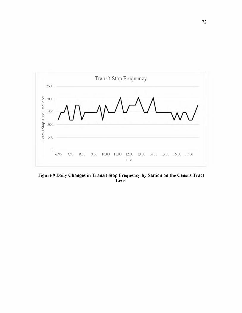
Tran
sit
Stop
Ti
me
Freq
uenc
y
72
Transit Stop Frequency2500
2000
1500
1000
500
0 ----------------------------------------------------------------------------------------------------------------------------6:00 7:00 8:00 9:00 10:00 11:00 12:00 13:00 14:00 15:00 16:00 17:00
Time
Figure 9 Daily Changes in Transit Stop Frequency by Station on the Census TractLevel
Accessibility between each pair of transit stations in the city was calculated as a part of
average accessibility calculations for public transit mode. These results are provided in
Figure 10, for different amounts of travel time budget. The percent of accessible transit
stations is then extracted as a ratio of transit station pairs accessible within a given time
over the total number of transit station pairs. As expected, the percent of accessible transit
stations increases as the users travel time budget increases. This is further confirmed with
the results provided in Figure 11, where transit accessibility dependence on the
acceptable walking time is given, and the results provided in Figure 12 where transit
accessibility varies with different amounts of the acceptable travel time spent in transit.
Incremental accessibility change is given in Figure 13 to show the combined effect of
changes in time spent on walking to and from a transit station, and time spent in public
transit, on the percent change in transit accessibility. All these and other factors that may
influence transit accessibility in urban environments are explained in a more detailed
manner in a previous study (Tasic et al., 2014). For the purpose of this research, it was
important to consider a wide range of potential variables that may have the influence on
safety outcomes, particularly nonmotorized safety outcomes in urban environments. All
calculated variables related to transit accessibility, however, were not included in the
final statistical models, and this will further be explained in the Results chapter.
Figure 14 shows spatial distribution of the average daily transit accessibility on the
census tract level. The results show relatively good coverage of the entire city by transit
service, where the downtown area of Chicago has the best access to destinations by
transit, as expected.
73

Num
ber
of Tr
ansit
Stop
Pa
irs
74
Transit Stop Accessibility
Access Time between Pairs of Transit Stops (min)
Figure 10 Number and Percentage of Transit Stops Accessible Within the GivenAmount of Time Budget

Ave
rage
N
umbe
r of
Des
tinat
ions
A
cces
sibl
e by
Tra
nsit
75
Transit Accessibility and Walking Time8000
7000
6000
5000
4000
3000
2000
1000
0OCOOCOOCOOCOOC^v o ' o r ^ i S o d o d c K c K o c
c o o c o o c o o c o o c o o c o o c o o c o o c ^
Time
5 min Walk Time 10 min Walk Time
15 min Walk Time 20 min Walk Time
Figure 11 Daily Variations of Transit Accessibility for All Census Tracts Dependent on Preferred Walk Time Within the 60-minute Available Time Budget
20:3
021
:00
21:3
0

76
Transit Accessibility and the Available Budget Time3000
eeagareevA
o m o m o m o m o m ' O ' o r ^ r ^ 6 6 6 o c ^ c ^ o o
m o m o m o m o m o m o m o m o m o m o m ^ < N ( N r :n r ^ ^ r ^ r ^ ^ ' 0 ' 0 t ^ r ^ 6 6 6 6 c ^ c ^ ....................
• 15 min budget Time
60 min Budget Time
■ 30 min Budget Time
90 min Budget Time
<N (N(N(N45 min Budget Time
120 min Budget Time
Figure 12 Daily Variations of Transit Accessibility for All Census Tracts Dependent on the Available Budget Time Within the 5-minute Walk from the Transit Stations

Num
ber
of A
cces
sibl
e D
estin
atio
ns
77
Incremental Accessibility Change12000 ------------------------------------------------------------------------------------------------------------------ 60%
10 15 20 25 30 45 60 90 120
Available B udget Time (min)
5 min Walk Access * 10 min Walk Access *15 min Walk Access * 20 min Walk Access
Figure 13 Incremental Change in Transit Accessibility Depending on the AvailableTime Budget and Walking Distance
Perc
ent
Chan
ge
in A
cces
sibi
lity

78
^ *ISi ■■■ ’r a J .B¥™ M in ■ ilH . .H U B K I5I55 bt- V
< 100
100 - 500
500 - 1000
1000 - 2000
> 2000 k
30 minute Travel Time by Transit
■■ slbrS Ih R A r
< 500
500 - 1000
1000 - 2000
2000 - 5000
> 5000
i p s r i i
90 minute Travel Time by Transit
< 500
500 - 1000
1000 - 2000
2000 - 5000
> 5000
60 minute Travel Time by Transit
< 1000
1000 - 2000
2000 - 5000
5000 - 10000
>10000
120 minute Travel Time by Transit
Figure 14 Destinations Accessible Within the Given Travel Time by Transit

When comparing these results to bicyclist accessibility, the number of destinations
accessible by bike appears higher than the number of destinations accessible by transit,
due to the fact that average time-dependent rather than total cumulative accessibility was
calculated for transit. While the developed accessibility indicators provide the basis for a
general multimodal accessibility indicator, calculation of such an indicator would require
making assumptions about user preference in terms of mode choice that are not strongly
supported by the data available in this study. As previously stated, the goal of the
developed indicators is to improve the way multimodal exposure is captured in the safety
prediction models, and development of a single indicator of multimodal accessibility
remains a part of future research efforts.
Explanatory Variables Representing System-wide Effects
Additional explanatory variables were developed using the available data on SE
characteristics and land use data to capture the system-wide effects that may influence
multimodal safety outcomes in urban environments. The final dataset included roughly
100 variables considered in the SASM analysis.
Socio-Economic Variables
The SE variables were drawn from the American Community Survey (ACS) 5-year
estimates of SE and household characteristics for each census tract in the City of Chicago
(U.S. Bureau of Census). The ACS data were aggregated on the census tract level,
allowing for a convenient extraction of variables of interest, without any need for the
additional data manipulation. The selection of the SE variables from the extracted ACS
data was based on the revised literature on traffic safety modeling in general, and traffic
safety modeling of spatially collected data.
79

The ACS provides single-year and multiyear estimates of SE and housing
characteristics of an area over a specific time period. The ACS collects survey
information continuously nearly every day of the year and then aggregates the results
over a specific time period: 1 year, 3 years, or 5 years. The data collection is spread
evenly across the entire period represented so as not to over-represent any particular
month or year within the period. Single-year data are more current, while multiyear data
are more reliable because of the larger sample size.
The primary uses of ACS estimates are to understand the characteristics of the
population of an area for local planning needs, make comparisons across areas, and
assess change over time in an area. Factors that guide users to determine which ACS
estimate to use where both single year and multiyear estimates are available include
intended use of estimates, precision of estimates, and currency of estimates. For small
geographic areas such as census tracts, 5-year ACS estimates are the only option, as
single-year and 3-year estimates are unavailable.
Both availability and accuracy of SE data from the ACS 5-year estimates influenced
the decision to use these estimates from the period from 2008 to 2012 and develop the SE
variables for the purpose of this research. The ACS 5-year data included population,
social, economic, and housing estimates on a variety of levels, and for this study, data are
extracted for the Illinois counties Cook and Du Page, for census tracts that belong to
Chicago. Figure 15 presents the spatial distribution of population density and
unemployment in Chicago. Descriptive statistics for SE variables is provided in Table 6.
80

81
Figure 15 Spatial Distribution of the Population Density and the Percent Unemployed Population in Chicago (U.S. Census ACS 5-Year Data, 2008 - 2012)

82
Table 6 Descriptive Statistics for the SE Variables
Variable Description Obs Mean Std. Dev. Min Max
Population Population Size 801 3.402 1.741 0.000 15.740
Pop_Dens Population Density per mile squared 801 18.203 20.206 0.000 485.019
Employed Percent of Employed Population 801 6.759 18.955 0.000 86.000
Unemploy Percent of Unemployed Civil Population 801 14.970 9.459 0.000 51.000
Total_HH Total Number of Households 801 1,296.553 786.911 0.000 9,180.000
HH_M ed Median Household Income 801 48,201.260 24,220.910 0.000 155,500.000
HHI_Mean Mean Household Income 801 65,296.570 35,266.030 0.000 211,891.000
FamI_Med Median Family Income 801 62,689.660 40,894.530 0.000 233,702.000
FamI_Mean Mean Family Income 801 82,579.100 59,415.360 0.000 394,284.000
PerCapInc Average Income per Capita 801 27,786.690 20,029.490 0.000 131,548.000
HH Total Number of Households 801 1,296.553 786.911 0.000 9,180.000
HHSize Average Household Size 801 2.707 0.709 0.000 5.560
FamSize Average Family Size 801 3.446 0.620 0.000 5.200
HHPop Population in Households 801 3,336.594 1,717.642 0.000 15,544.000
ED9 No High School Degree, % 801 9.644 10.061 0.000 51.900
ED9_12 Some High School, % 801 10.460 7.166 0.000 38.400
EDHigh High School Degree, % 801 23.717 11.402 0.000 58.600
EDSomeCol Some College, % 801 18.898 8.292 0.000 48.700
EDAssoc Associate Degree, % 801 5.477 3.236 0.000 34.600
EDBach Bachelor's Degree, % 801 18.820 14.157 0.000 70.200
EDGrad Graduate School Degree, % 801 12.483 12.291 0.000 63.900
EDHighPlus More than High School Degree, % 801 79.396 15.181 0.000 100.000
EDBachPlus More than Bachelor's Degree, % 801 31.303 25.240 0.000 96.900
HousUnits Number of Housing Units 801 1,506.150 890.775 0.000 10,906.000
HousOcc Occupied Housing Units, % 801 84.862 11.109 0.000 100.000
NoVeh Households with no Vehicles, % 801 26.537 15.118 0.000 89.400
Veh1 Households with 1 Vehicle, % 801 43.589 9.508 0.000 81.300
Veh2 Households with 2 Vehicles, % 801 22.558 11.544 0.000 59.100
Veh3plus Households with 3 or more Vehicles, % 801 6.814 5.648 0.000 26.900

83
Land Use Variables
Land use has emerged as an important factor to consider in any type of transportation
analysis, particularly in urban environments. CMAP provided land use data for this
research, in the form of digital geospatial polygon parcel data that indicate land use in
northeastern Illinois.
Numerous GIS reference layers and several internet resources are used to support the
land use inventory that is updated periodically. This research initially used land use data
for the year 2005, which were available as polygon data that did not account for the right
of way. After the initial research proposal, new land use data for the year 2010 became
available for the analysis. Land use data from 2010 are parcel-based, account for the
transportation right of way, and represent more accurate details on how land use is
distributed spatially in Chicago. Therefore, this research used the most recent land use
data for 2010 from CMAP. Land use variables are given in Table 7. Land use diversity
was calculated as the total number of different land uses within each census tract, where
eight categories of land uses were established: residential, commercial, institutional,
industrial, transportation, agriculture, open space, and vacant (under construction). Land
use entropy (Figure 16) is a measure of land use balance developed and used in previous
studies (Wang and Kockelman, 2013; Cervero and Kockelman, 1997), and calculated as:
Equation (8)
Where:
pi - the proportion of land use “i" in the census tract area
n - the maximum number of land uses in census tract (in this case n = 8)

Table 7 Descriptive Statistics for Land Use Variables
84
Variable Description Obs Mean Std. Dev. Min Max
Figure 16 Land Use Parcels and Land Use Entropy in Chicago

Statistical Areal Safety Modeling Methods
This section of the Methodology chapter is focused on explaining the SASM
methodology used to estimate multimodal crash outcomes on the census tract level using
the dataset from Chicago based on the variables described in the previous sections of this
chapter. The chapter includes the framework used for the application of SASM
methodology, the description of five different SASM methods, and the diagnostics used
to evaluate these methods. As shown in Figure 17, the application of SASM methods for
the previously defined response and explanatory variables started from the traditional
crash prediction models, and expanded to frequentist and Bayesian methods that account
for spatial effects potentially present in the data. Due to the fact that data are spatially
collected and aggregated, adequate tests for spatial auto-correlation were conducted. The
combination of R, STATA, and ArcGIS was used to execute the SASM methodology
presented in this section.
Frequentist Approach to Crash Modeling
There are two main approaches to statistical inference used to model crash data over
the previous decade, frequentist and Bayesian. The key difference between these two
approaches in in the way unknown parameters are defined and estimated. When
frequentist statistical inference is used, it is assumed that data are a repeatable random
sample, the hypothesis is fixed (either true or false), and parameters are considered to
remain constant during the sampling process. This inferential approach is called
frequentist because it is focused on the expected frequency with which the data will be
observed, given the defined hypothesis.
85

86
Response Variables (Expected number of crashes}
Explanatory Variables {Exposure,, Accessibility, System-wide effects)
Exploratory Data Analysis (Response and Explanatory Variables)
Spatial Autocorrelation Tests
GlobalAutocorrelation
LocalAutocorrelation
Statistical Areal Crash Modeling (SASM)
r ^Frequentist BayesianInference
k. j
8 ." - Inference
Generalized Linear Models
. A
r iGeneralized
Additive ModelsJ
r
Full Bayes Hierarchical Models
Figure 17 Flowchart of Crash Data Analysis Process

Bayesian approach uses probability to describe the unknown parameters, recognizing
the uncertainty that exists in the knowledge about the parameters that should be
estimated. Unlike the frequentist approach, Bayesian statistics is focused on determining
the probability of the hypothesis, given the observed data, so while data are considered to
be fixed, hypothesis is considered to be random.
Areal safety studies have been conducted using both frequentist and Bayesian
estimation methods. Particularly over the last 10 years, Bayesian statistics became
predominant in SASM, due to limitations of frequentist methods to capture spatial
autocorrelation and heterogeneity of crash data. This research was conducted using both
frequentist and Bayes SASM. While previous studies mostly use frequentist approach
based on GLM, this study also explored the potential of GAM to capture the unobserved
shared effects between analyzed areas (census tracts). In addition, Full Bayes
Hierarchical (FBH) were also used to see if the estimated parameters obtained from both
frequentist and Bayesian inference are comparable in terms of values and significance
levels.
As crash data are positive count data, the primary statistical modeling approach based
on frequentist inference is Negative Binomial (NB) regression, as a more general
variation of Poisson regression which can account for overdispersion often present in
crash data (Hilbe, 2007). The NB model includes an error term, , for which the
exponent, exp(£j), follows a gamma distribution with parameters (1, a), where a is the
overdispersion parameter. The general form of Negative Binomial model is (Hilbe,
2007):
^ = g(.Po+Pi in(Expii)+^2 in(Exp2i)+S/Pj xij+£{) Equation (9)
87

Where:
0; - expected number of crashes for census tract “i”
P0-intercept
Pi - coefficients quantifying the effect of the “j ” explanatory variables characterizing census
tract “i” on 0;
Expl and Exp2 - measures of exposure in census tract “i”
x; - a set of “j ” explanatory variables that characterize census tract “i” and influence 0;
si - disturbance term corresponding to census tract “i”
In the NB model provided in Equation 10, the variance in the number of crashes is:
0j + tfjS2. The provided general form of the NB model from the Equation 10 can further
be expanded to capture SASM of the expected number of crashes for vehicular,
pedestrian, and bicyclist users:
6 veh i = e (p0 +Pi ln(DVMT) + ^ 2 in(Road)+zJPJ xij+si) Equation (10)
@ped i = e (@o+Piln(DVMT)+P2 ln(Ped)+'ZjPj xij+si) Equation (11)
Obike i = e (Po+Piln(DVMT^+p2 WBm+XjPjXi j+et i Equation (12)
In the case of the SASM method developed for estimating the number of total and
severe vehicular crashes, both DVMT and length of road (variable “Road”) were used as
measures of exposure, to capture both the presence of vehicular users and the relationship
between the road network mileage and DVMT on the census tract level. The SASM
method used to estimate the expected number of total and severe pedestrian crashes
(Equation 12) uses both DVMT and the number of generated pedestrian trips in the
census tract as units of exposure. The SASM method used to estimate the expected
number of total and severe bicyclist crashes (Figure 13) uses DVMT and the number of
88

generated bicyclist trips to represent bicyclist users exposure to crashes in census tracts.
The ASM methods based on other statistical modeling techniques (GLM, GAM, FBH)
used the same framework to represent the exposure. The main assumption behind the
exposure incorporated in the SASM models in this way was that if the exposure of one of
the two conflicting modes was zero, it was expected that the number of crashes would be
zero as well.
The NB models presented in the Equations 10-13 above do not account for the
presence of spatial autocorrelation in the data, which may be a limitation to adequately
representing the data generating process, particularly when data are spatially aggregated
and the number of crashes in one area may depend or be similar to the number of crashes
in the areas nearby (i.e., a spatial spillover effect). In cases where spatial autocorrelation
is present, it may increase the variance of estimated parameters, while their standard
errors may be underestimated by the NB model (Aguero-Valverde & Jovanis, 2006;
Quddus, 2008). In such cases, the NB model can be modified through an additional term
that is added to the model to represent spatial random effects in the data.
Detecting Spatial Autocorrelation
The NB model is estimated using the maximum likelihood approach, constructed on
the basis of the assumption that the observations in the model are independent. This
assumption does not hold when data are clustered (Anselin, 2013). Clusters appear in the
case when spatial correlation is present in the dataset, where nearby entities are related
more than the entities that are far apart (Greene, 2003).
It is previously acknowledged that due to shared spatial effects, crash data have the
tendency for clustering (Aguero-Valverde & Jovanis, 2006). In addition, the way data are
89

90
organized and aggregated, rarely follows the actual cluster boundaries (Anselin, 2013). In
the case of the dataset built for the purpose of this research, census tracts are not very
likely to match the spatial agglomeration of the crashes, contributing to the additional
bias in the modeling process. Several measures of spatial autocorrelation may be utilized
to indicate the existence of clusters in the dataset, including Moran’s I, Getis-Ord’s G,
and Geary’s C (Anselin, 2013). Due to its broad application and the convenience of
interpretation, Moran’s I was used in this research as the indicator of global and local
auto-correlation.
Global Moran’s I measures the general tendency to clustering based on location of an
entity and the values of the selected entity’s attributes. The Global Moran’s Index value
with z-score and p-value that indicate the significance of the index is calculated as
follows (Anselin, 2013):
_ n 'Zi=i'L1 j= i W iJz iZj Equation (13)= S TV- z?
Where:
n — total number of entities
zi — deviation of an attribute from its mean
wi,j — spatial weight between features i and j
i = l j = l
I —E[I]Zj = _ _
Equation (14)

Where:
E[l] = —1 / ( n — 1)
V [ l ] = E [ l 2 ] —E[ l ] 2
The Global Moran’s I is interpreted in terms of its null hypothesis which states that the
analyzed attribute is randomly distributed among the entities of interest. One of three
alternative assumptions about the data may be made when Moran’s I test is applied to
detect spatial autocorrelation: normality, randomization, or no assumptions (Acevedo,
2013). If the data are a part of a known larger trend, where the values of the variable in
each region are drawn from the same normal distribution, and the mean and the variance
are the same for all regions, the normality assumption may be used. If the data are close
to normally distributed, but the trend is unknown, it can be assumed that all permutations
of the values of the variable are equally likely, and the randomization assumption may be
used. When the previous two assumptions cannot be made about the data, Monte Carlo
simulation of Moran’s I may be used (Acevedo, 2013). While previous studies of crash
data used Moran’s I to detect and measure spatial autocorrelation, it is rarely indicated
under which assumptions the test was conducted (Moeinaddini et al., 2014;
Yiannakoulias et al., 2012).
In this research, prior to conducting the Moran test, neighborhood functions between
census tracts were created using boundary methods. Spatial weights were then assigned
by using the inverse distance method. Global spatial autocorrelation was detected by
using a Monte Carlo method, where data are rearranged several hundred times by re
assigning the values of the variable of interest (vehicular, pedestrian, and bicyclist
crashes) to different spatial units and obtaining several hundred random spatial
91

distributions of that variable. Moran’s I is then calculated for each of these arrangements,
and these simulated values are used to construct a simulated sample distribution. Then the
observed value of Moran’s I obtained from the original data arrangement is compared to
this distribution obtained from random sampling, and if it exceeds 95% of simulated
values, it is very likely that the observed distribution is significantly autocorrelated. In
this case, the null hypothesis of spatial randomness is rejected.
This test is not two-sided, due to the fact that ranking is used, so either positive or
negative autocorrelation should be assumed. In this case, the Monte Carlo method was
applied to the data with the assumption of positive autocorrelation, the most common
scenario (Acevedo, 2013). As the Monte Carlo test is distribution-free, crash-related
variables on the census tract level did not need to be transformed. The tests were run with
1000 simulations and the plotted results are provided in Figure 18 and Figure 19.
Although the values of the Moran statistics are low and would seem to indicate no spatial
pattern, the Z-value is high due to low variance and the p-value of the hypothesis test is
low, indicating that spatial autocorrelation is very likely present in the data. Modeling
methods explained in the following parts of the paper attempt to account for the presence
of spatial autocorrelation in the data.
Since the global indicator of spatial correlation shows general tendency to clustering
in the dataset, local Anselin Moran’s Index was utilized to measure the degree of
similarity between neighboring census tracts (Anselin, 2013). The calculations were
based on several different neighborhood definitions for the local Moran’s I calculations.
The results of the local auto-correlation test should show potential presence of clusters of
high values, low values, and spatial outliers for vehicular and nonmotorized crashes on
92

93
Vehicle-only Crashesnumber of simulations + 1:1000 statistic = 0.2948 observed rank = 1000 p-value = 0.001alternative hypothesis: greater (rejected null hypothesis)
Pedestrian Crashesnumber of simulations + 1:1000 statistic = 0.3344, observed rank = 1000, p-value = 0.001alternative hypothesis: greater (rejected null hypothesis)
Bicyclist Crashesnumber of simulations + 1:1000 statistic = 0.3743, observed rank = 1000, p-value = 0.001alternative hypothesis: greater (rejected null hypothesis)
Figure 18 Monte Carlo Simulation of Moran’s I for Total Multimodal Crashes

94
Vehicle-only KA Crashesnumber of simulations + 1:1000 statistic = 0.2011 observed rank = 1000 p-value = 0.001alternative hypothesis: greater (rejected null hypothesis)
Pedestrian KA Crashesnumber of simulations + 1:1000 statistic = 0.2283, observed rank = 1000, p-value = 0.001alternative hypothesis: greater (rejected null hypothesis)
Bicyclist KA Crashesnumber of simulations + 1:1000 statistic = 0.2177, observed rank = 1000, p-value = 0.001alternative hypothesis: greater (rejected null hypothesis)
Figure 19 Monte Carlo Simulation of Moran’s I for Severe (KA) Crashes

the census tract level. Further methods were developed based on the traditional crash
prediction techniques and these preliminary measurements of spatial dependence. The
results of local Moran’s Index are provided in Figure 20.
Generalized Linear Models
GLM are a flexible generalization of linear regression models that allow for response
variables that have distribution other than normal. The previously described negative
binomial model is considered to be a generalized linear model, and it may take some
extended forms to accommodate random effects existing in spatially collected crash data.
Two such forms, negative binomial with fixed effects and with random effects, are
described in this section of the crash data analysis methodology.
While global Moran’s I indicates the presence of spatial correlation in the data, local
Moran’s I identifies clusters of census tracts with similar (high or low) crash frequencies
(Figure 20). These results indicate that crash models need to be developed to account for
spatial correlation and acknowledge clustering in the dataset. Previous research also used
local Moran’s I results to spatially aggregate contiguous units of analysis in road safety,
often for the purpose of identifying crash hot-spots (Huang et al., 2009; Miranda-Moreno
et al., 2007).
After determining the presence of spatial correlation in the dataset using global
Moran’s I, the results of local Moran’s I test were utilized to aggregate census tracts into
higher level spatial categories that would approximately capture the identified clusters
through the assignment of fixed and random effects to these groups within the NB model
framework.
95

96
Figure 20 Local Moran’s I Results
This is similar to building neighborhood structure in spatial auto-regression models for
normal data and the approach has already been used in previous research, but considered
only models with fixed effects (Wang et al., 2009). The NB model can account for spatial
correlation if it is formulated in a way that includes an additional parameter that would
represent the spatial dependence (Greene, 2003). This additional parameter for clustered
data can be introduced through fixed or random effects panel models (Hilbe, 2007; Lord
& Mannering, 2010). The fixed effects NB (FENB) model can be estimated as an
unconditional or conditional model (Hilbe, 2007). The conditional FENB has the ability
to accommodate a large number of panel units, but it has been questioned by some, as it
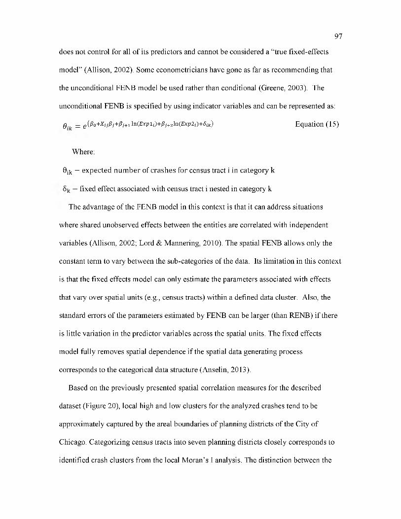
does not control for all of its predictors and cannot be considered a “true fixed-effects
model” (Allison, 2002). Some econometricians have gone as far as recommending that
the unconditional FENB model be used rather than conditional (Greene, 2003). The
unconditional FENB is specified by using indicator variables and can be represented as:
$ = e {Po+XijPj+Pj+iin{ExpiC>+Pj+2 in(Exv2 {)+8 ik) Equation (15)
Where:
0ik — expected num ber of crashes for census tract i in category k
— fixed effect associated with census tract i nested in category k
The advantage of the FENB model in this context is that it can address situations
where shared unobserved effects between the entities are correlated with independent
variables (Allison, 2002; Lord & Mannering, 2010). The spatial FENB allows only the
constant term to vary between the sub-categories of the data. Its limitation in this context
is that the fixed effects model can only estimate the parameters associated with effects
that vary over spatial units (e.g., census tracts) within a defined data cluster. Also, the
standard errors of the parameters estimated by FENB can be larger (than RENB) if there
is little variation in the predictor variables across the spatial units. The fixed effects
model fully removes spatial dependence if the spatial data generating process
corresponds to the categorical data structure (Anselin, 2013).
Based on the previously presented spatial correlation measures for the described
dataset (Figure 20), local high and low clusters for the analyzed crashes tend to be
approximately captured by the areal boundaries of planning districts of the City of
Chicago. Categorizing census tracts into seven planning districts closely corresponds to
identified crash clusters from the local Moran’s I analysis. The distinction between the
97

Central district and the other planning districts in terms of crash concentration is
noticeable. This potential categorical structure of the data with the existing planning
districts as categories and the census tracts as observations led towards exploring the
FENB model with indicator variables for planning districts as the one possible way to fit
the data and account for spatial dependence.
Random effects NB models (RENB) are another option for trying to capture the spatial
level heterogeneity in the dataset. The main assumption with the random effects model is
that the unobserved shared effects among defined spatial entities are uncorrelated with
the explanatory variables. If this is the case, the random effects estimator is consistent
and estimated parameters will have smaller standard errors than the fixed effects model.
The random parameter in RENB model typically follows Gaussian, inverse Gaussian, or
preferably gamma distribution (Greene, 2003; Hilbe, 2007). The general form of the
RENB model is similar to the form of FENB model (Hilbe, 2007):
$ = e (Po+^ijPj+Pj+iin(Expii)+pj+2 in(Exp2 i)) e ^ik Equation (16)
Where:
n ik — random effects for observation i nested in category k
Generalized Additive Models
GAM represent another modeling technique that uses frequentist approach in
estimating model parameters. Generalized additive models were introduced by (Hastie &
Tibishirani, 1990), as an additive extension of the family of generalized linear models.
These models were developed with linear predictors, just as generalized linear models,
but with also including a sum of smoothing functions of explanatory variables. Since a
smoothing function is a tool for summarizing the trend of a response measurement as a
98

function of one or more explanatory variables, generalized additive models allow for a
more flexible specification of the dependence of the response on the explanatory
variables (Hastie & Tibishirani, 1990; Wood, 2006). Generalized additive models replace
the linear form “fa0 + fa x t” by the additive form “f a + % i f ( x{) " (Hastie &
Tibishirani, 1990). Generalized linear models are estimated by computing the maximum
likelihood estimates, as an iteratively reweighted least-squares procedure. This procedure
is modified for the estimation of generalized additive models where the parameters are
estimated by penalized likelihood maximization (Hastie & Tibishirani, 1990; Wood,
2006). The general additive model structure for the case of negative binomial distribution
is as follows (Hastie & Tibishirani, 1990):
$ = e (Po+Y.jfj{ xij)+Ei) Equation (17)
Where:
0 i - expected number of crashes for census tract “i”
P0- intercept
fj - smooth function quantifying the effect of the “j ” explanatory variables characterizing
census tract “i” on 0 i
x ij - a set of “j ” explanatory variables that characterize census tract “i” and influence 0i
- disturbance term corresponding to census tract “i”
An additive model may have component functions with two or more dimensions
(Hastie & Tibishirani, 1990). If a smoothing function is used across the locations on
spatially aggregated data, generalized additive models may be used to represent spatial
processes in the data and account for spatial variation. While two previous applications of
additive models in crash studies developed smoothing functions related to explanatory
99
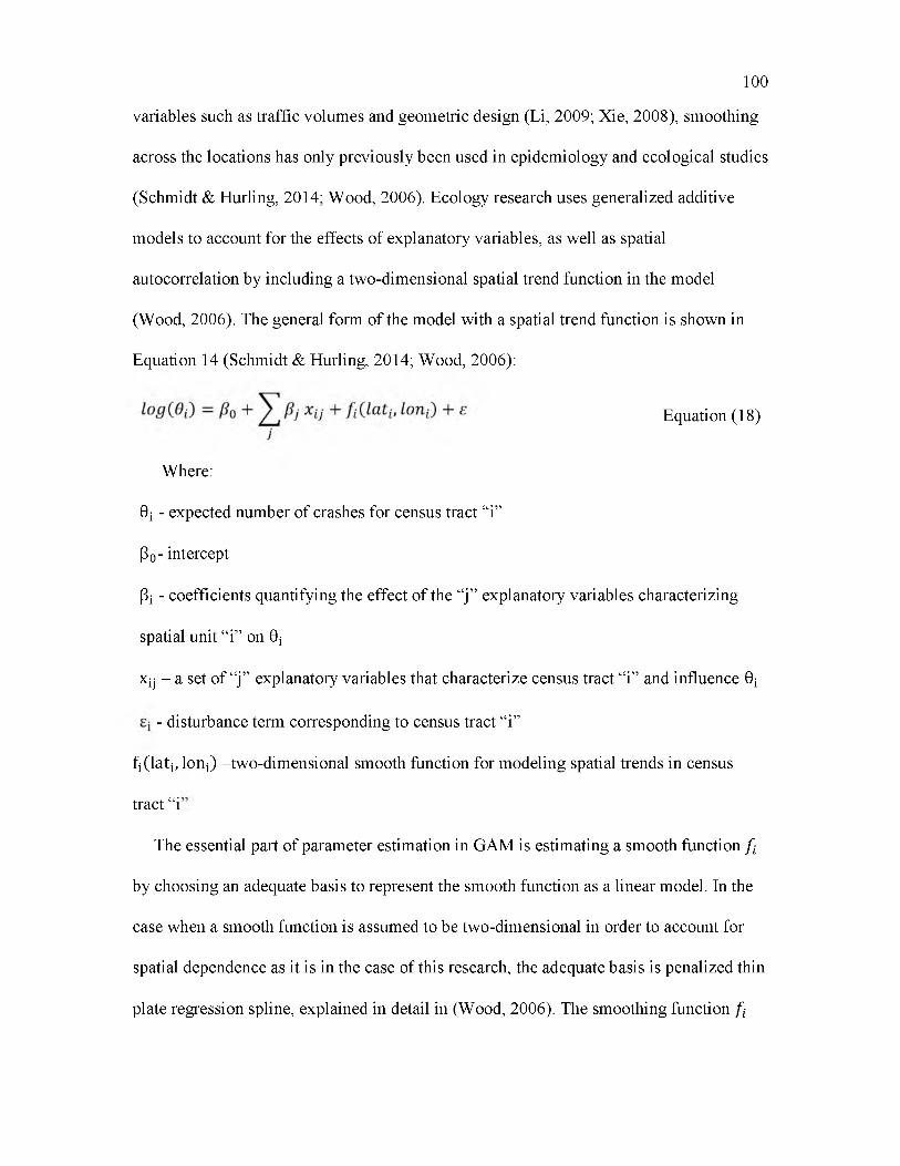
100
variables such as traffic volumes and geometric design (Li, 2009; Xie, 2008), smoothing
across the locations has only previously been used in epidemiology and ecological studies
(Schmidt & Hurling, 2014; Wood, 2006). Ecology research uses generalized additive
models to account for the effects of explanatory variables, as well as spatial
autocorrelation by including a two-dimensional spatial trend function in the model
(Wood, 2006). The general form of the model with a spatial trend function is shown in
Equation 14 (Schmidt & Hurling, 2014; Wood, 2006):
Where:
0i - expected number of crashes for census tract “i”
P0- intercept
Pi - coefficients quantifying the effect of the “j ” explanatory variables characterizing
spatial unit “i” on 0 i
x ij - a set of “j ” explanatory variables that characterize census tract “i” and influence 0i
- disturbance term corresponding to census tract “i”
fi(la ti, loni) -two-dimensional smooth function for modeling spatial trends in census
The essential part of parameter estimation in GAM is estimating a smooth function ft
by choosing an adequate basis to represent the smooth function as a linear model. In the
case when a smooth function is assumed to be two-dimensional in order to account for
spatial dependence as it is in the case of this research, the adequate basis is penalized thin
plate regression spline, explained in detail in (Wood, 2006). The smoothing function ft
Equation (18)
tract “i

used in this research is estimated by minimizing the following penalized least square
function:
m i n Y j ( y l —f i) 2 + X! mA( f ) Equation <19>i
Where:
yi- observed number of crashes in census tract “i”
fi- thin plate regression spline smoothing function for modeling spatial trends in census
tract “i”
X- smooth term resulting from GAM estimation
Jm,d(f)- penalty function measuring the roughness of the f estimate
The type of model setting represented in Equation 17 assumes that spatial dependence
can be handled by including it in the systematic part of the model, similar to modeling a
lag effect. The additive regression models were fitted with a two-dimensional smoothing
function of the geographic location of each spatial unit of analysis, to capture the spatial
autocorrelation and nonlinear effects which could not be captured by the observed
explanatory variables (Schmidt & Hurling, 2014; Wood, 2006). Whether this approach is
appropriate to model the existing spatial autocorrelation in the data depends on the
complexity of spatial dependence. GAM with smoothing splines across the locations
essentially models the trend in the autocorrelated data while other explanatory variables
represent the deviation from this trend. The advantage of GAM models is that they allow
for more complex trends than a simple trend surface. Modeling spatial dependence
between observations in this manner reduces the possibility of residuals being
autocorrelated and violating the assumptions of independence. In the cases of datasets
where the error terms are stronger sources of autocorrelation, alternative methods should
101

be applied to ensure that there the estimated coefficients and standard errors are not
biased.
102
Bayesian Approach to Crash Modeling
Bayesian statistical inference offers an alternative to frequentist approach that uses a
hypothesis testing framework and reports p-values to indicate the significance of
estimated parameters. Bayesian methods have gained a lot of interest in the area of
SASM over the previous decade, due to their ability to incorporate prior information in
modeling process and parameter estimation. Bayesian approach includes modeling of
both observed data and any unknowns as random variables, providing a comprehensive
framework for combining prior knowledge with complex data models.
In the case of Bayesian models, in addition to specifying f ( y \ f i ) , for the set of
observations y = { y 1, y 2, ... y n}, for the vector of unknown parameters fa =
[P 1 , P 2, —Pn}, it is considered that fa is a random quantity sampled from a prior
distribution n( P \ r ) , where t is the vector of hyper-parameters, controlling how fa truly
varies. When x is known, the inference about fa is based on the posterior distribution,
given by the Bayes theorem:
(a \ 1 = P & ' P W P & P W f (y \ P ' ) ^ (P\^) Equation (20)P ( m ' T) p ( y \ T) f p ( y , f a l z ) d f a S ( y l P) K( f i \ T ) dp
Where:
p — conditional probability
f - likelihood function
n — external knowledge prior

The Bayesian inference based on the theorem given in Equation 19 is considered to
provide advantages over the frequentist inference as it includes a knowledge-based
foundation through the incorporated priors. Another advantage of Bayesian framework is
that it allows modeling parameters fa with random instead of fixed effects and allows the
introduction of structures that capture spatial auto-correlation in the models, which is
why Bayesian inference usage in statistical crash modeling significantly increased as the
need to model crashes on the macroscopic level appeared.
Full Bayes Hierarchical Models
Based on the previously reviewed literature, spatial safety analysis was conducted by
either applying the traditional models such as NB variations, and models with Bayesian
inference. The advances in computing methods and the inability to estimate maximum
likelihood function for data with less common distributions led to increased use of
Bayesian estimating methods (Lord & Mannering, 2010). Bayesian approach allows the
usage of sampling-based simulation methods to estimate more complex model forms,
particularly when data exhibit spatio-temporal correlations (Huang & Abdel-Aty, 2010;
Kim et al. 2007).
Previous studies found that the results of the safety analysis based on frequentist and
Bayesian inference both agree or disagree (Aguero-Valverde & Jovanis, 2006; Quddus,
2008; Siddiqui et al., 2012; Wang & Kockelman, 2013). Certain authors recommend the
exclusive application of Bayesian models, considering that they are flexible enough to
account for both spatial effects and overdispersion (Huang & Abdel-Aty, 2010; Quddus,
2008;). Other authors found that frequentist and Bayesian models yield similar
conclusions (Aguero-Valverde & Jovanis, 2006). Some authors consider that the
103

complexity of Bayesian methods is a serious barrier to their application (Lord &
Mannering, 2010).
Developing SASM under Bayesian framework has become more frequent over the
past several years, as the computational capabilities increased to allow for more complex
modeling processes (Lord & Mannering, 2010). Spatial autocorrelation issues may be
resolved in models developed under Bayesian framework if spatial heterogeneity is
accounted for through incorporation of Conditional Autoregressive (CAR) or Spatial
Autoregressive (SAR) models. The majority of previous road safety studies use CAR
model because of its suitability for the analysis of geographic regions (Wang &
Kockelman, 2013). The combination of NB model and CAR model cannot be estimated
by using maximum likelihood, and it has to be estimated by using Monte Carlo Markov
Chain (MCMC) simulation (Park & Lord, 2007).
A Bayesian hierarchical model with Conditional Autoregressive (CAR) prior was used
in this research, in order to compare the results obtained from previously explained
modeling methods. This model is proposed by (Besag, 1975), and used by (Aguero-
Valverde & Jovanis, 2006; Quddus, 2008). Acknowledging that more complex Bayesian
models with more informative priors have been developed over the past several years
(Wang et al., 2014), this paper uses the model with highly noninformative priors for
parameter estimates, in order to provide a comparison between the estimates resulting
from the Bayesian approach and models with frequentist inference explained in previous
sections of this chapter.
In the Bayesian hierarchical model, the posterior distribution of all unknown
parameters is proportional to the product of the likelihood and the prior distributions
104

105
(Aguero-Valverde & Jovanis, 2006; Quddus, 2008). The modeling approach assumes that
crash counts have Poisson distribution:
Where:
yi-observed number of crashes in entity i
0i- expected mean of total crash frequency for entity i
P0- intercept, assumed uniform distribution
Pi- coefficients, assumed normal prior ~N(0,1000)
X] - explanatory variables influencing 0i
^ - spatially correlated random effect for entity i
U - unobserved heterogeneity among entities
Spatial dependence among entities, in this case census tracts, is incorporated through
the CAR prior (Besag, 1975), which follows normal distribution with mean and variance
The term w tj is 1 if entities “I” and “j ” are adjacent, and 0 otherwise, while tv controls
the variance of spatial correlation, and has the assumed prior Gamma distribution
r v~Ga(0.5,0.0005). The unobserved heterogeneity among entities is assumed to follow
a normal distribution, Ui ~N( 0 , tu2); where xu is the parameter that controls Poisson
extra-variation with a prior Gamma distribution r u~Ga(0.5,0.0005), as previously used
in (Aguero-Valverde & Jovanis, 2006; Quddus, 2008). The Bayesian hierarchical model
y i~ P o i s s o n ( 6 i) Equation (21)
Equation (22)
N(Si'Ti):
Equation (23)

was estimated using a Markov Chain Monte Carlo method (MCMC), with 10,000
iterations where the first 2,000 iterations were removed as burn-ins.
Preliminary and Final Model Specifications
The SASM methods explained in this chapter were applied towards the estimation of
the expected number of crashes for six identified response variables: total vehicular
crashes, severe vehicular crashes, total pedestrian crashes, severe pedestrian crashes, total
bicyclist crashes, and severe bicyclist crashes. As the dataset built for the purpose of this
research includes roughly 100 variables, including all independent variables in
preliminary model specifications was not feasible. Instead of including all defined
variables in the preliminary models, the SASM process started with including different
sets of variables. This way, preliminary models were developed including variables that
showed higher significance level across various sets of model specifications, consistent
sign and magnitude, and appeared in the previous research studies that used SASM
methodology.
Preliminary statistical models were developed by running NB models only, rather than
running all types of models described in the previous chapter. The reasoning behind the
modeling process initiated this way is that given the modeling methods features, NB
models were most likely to overestimate the significance of variables included in
specifications. It is typical to use this approach and apply less complex SASM models
first in order to explore many possible specifications. After using negative binomial
models to obtain preliminary specifications, final model specifications were obtained for
all modeling methods and all outcome variables. The variable selection process that led to
obtaining the final model specifications was carried out by looking at the p -values and the
106

significance of each variable, by relying on the previous research done and the reviewed
literature, and by considering logical relationships that were expected to be found
between the independent and dependent variables. In addition, once the model
specification became close to final, several different SASM methods were applied to the
same specification to obtain the most consistent set of variables.
Diagnostics and Final Model Recommendations
After obtaining final model specifications for all six response variables, based on the
process described in the previous section, results from all five SASM methods applied in
this research were evaluated in order to recommend the final model for each of the six
response variables. The combination of model-specific parameters, goodness of fit
measures, and overall comparison of estimated parameters for the explanatory variables
was used to recommend the final six SASM models. Model-specific parameters that were
used as the preliminary indicators of performance for each SASM method applied in this
research included the following:
• Alpha: The over-dispersion parameter in the NB models accounting for the fact
that crash data variance is greater than the mean
• Pseudo R2: Pseudo r-squared is calculated as {1 — LL(™-od£l\LL(ilU.ll)
• LL: The value of the log likelihood function of the final model
• Ln(r), Ln(s): Beta distribution parameters, where ( 1 / 1 + a l pha) follows
Beta (r, s ) distribution
• Smooth terms: Two-dimensional smooth function parameters based on penalized
thin-plate regression splines. Coefficient estimates of smooth terms provided with
107

standard errors and p-values indicate statistical significance of smooth functions
included to account for spatial autocorrelation
• Deviance explained: The percentage of deviance explained, based on the sum of
squares of the deviance residuals, as the model deviance, and the sum of squares
of the deviance residuals when the covariate effects are set to zero, as the null
deviance
• Adj. R2: Adjusted r-squared as the proportion of variance explained in GAM
models
• REML: The value of restricted (or penalized) maximum likelihood function in
GAM models
• Tau2: Spatially correlated random effects in FBH models
• Sigma2: The variance of unobserved heterogeneity in the data in FBH models
• %accept: The probability of acceptance for the parameters in FBH models.
In addition, more general measures of model goodness of fit were calculated for all
SASM methods applied in this research. These measures were calculated for all five
SASM methods applied to estimate the expected number of crashes for six defined
response variables. These diagnostics measures included the following:
• Akaike Information Criterion (AIC) is a measure of information lost using a
specific model to represent the data generating process. Lower AIC values
indicate better model goodness of fit. It is calculated as follows:
AIC = 2 Pd — 2LL Equation (24)
Where:
108
P- the number of estimated model parameters
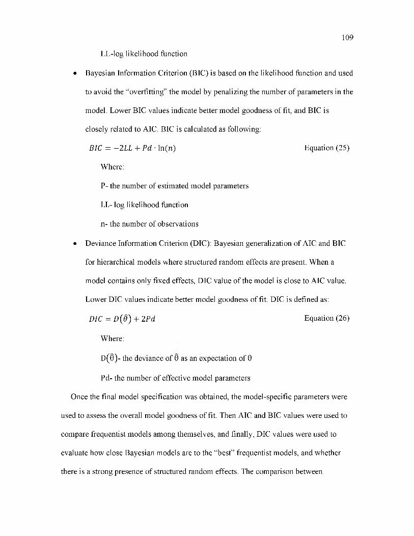
LL-log likelihood function
• Bayesian Information Criterion (BIC) is based on the likelihood function and used
to avoid the “overfitting” the model by penalizing the number of parameters in the
model. Lower BIC values indicate better model goodness of fit, and BIC is
closely related to AIC. BIC is calculated as following:
BIC = —2LL + Pd • ln(n) Equation (25)
Where:
P- the number of estimated model parameters
LL- log likelihood function
n - the number of observations
• Deviance Information Criterion (DIC): Bayesian generalization of AIC and BIC
for hierarchical models where structured random effects are present. When a
model contains only fixed effects, DIC value of the model is close to AIC value.
Lower DIC values indicate better model goodness of fit. DIC is defined as:
DIC = D ( § ) + 2 Pd Equation (26)
Where:
D (0)- the deviance of 0 as an expectation of 0
Pd- the number of effective model parameters
Once the final model specification was obtained, the model-specific parameters were
used to assess the overall model goodness of fit. Then AIC and BIC values were used to
compare frequentist models among themselves, and finally, DIC values were used to
evaluate how close Bayesian models are to the “best” frequentist models, and whether
there is a strong presence of structured random effects. The comparison between
109

Bayesian and frequentist models cannot be directly made, but the estimated coefficient
values and standard errors were used to determine whether frequentist models can serve
as a valid alternative in SASM process. The results of the applied SASM methods are
presented in the following chapter.
110

CHAPTER 4
STATISTICAL AREAL SAFETY MODELING RESULTS
This chapter presents the results of the SASM analysis methods. The results are
presented by crash type, for each of the six crash types which were the focus of the
analysis, and include the estimates obtained using all SASM methods described in the
previous chapter. Preliminary and final model specifications were obtained using the
approach for carrying out the variable selection described in the previous chapter. While
preliminary model specifications are shown only for negative binomial models, final
model specifications are shown for all crash types and all applied SASM methods
including NB models, FENB and RENB models, GAM, and FBH models. The presented
models include the method-specific goodness of fit indicators and the diagnostics used to
evaluate all applied SASM methods for different crash types. The final models for each
crash type are recommended based on the comparison of the final model specification
estimated from different SASM methods. The end of this chapter is dedicated to the
results extracted to demonstrate the effects of multimodal trips and multimodal
accessibility on the multimodal crash outcomes estimated from the final model selection.
The interpretation of the results presented in this chapter is provided in the following
Discussion chapter.

Preliminary Model Specifications
Six dependent variables were modeled in the described SASM process, including the
expected number of total vehicular crashes, severe vehicular crashes, total pedestrian
crashes, severe pedestrian crashes, total bicyclist crashes, and severe bicyclist crashes.
Tables 8 and 9 show the preliminary model specifications, based on negative binomial
models. The preliminary models provided in Tables 8 and 9 were further used to obtain
final model specifications for estimating each response variable. The coefficients
estimated in preliminary models provided indications about the sets of variables that
potentially may be a part of specifications that would adequately represent the data
generating process.
Table 8 Preliminary Specification of NB Model Used to Obtain Final Model Specifications for Total Vehicular, Pedestrian, and Bicyclist Crashes
Model Vehicle-only eras h model Pedestrian crash model Bicyclist crash model
Variable Coef. Std. Err. Pr(>iz|) Coef. Std. Err. Pr(>lzj) Coef. Std. Err. Prdzl)Population density (per mile2) 0.0000 0.0000 0.000 0.0000 0.0000 0.000 0.0000 0.0000 0.000Unemployed Population (°b) -0.0023 0.0019 0.229 0.0114 0.0030 0.000 -0.0280 0.0033 0.000In (Road miles) 0.9654 0.0666 0.000 1.1561 0.1043 0.000 0.7373 0.1175 0.000In (DVMT) 0.2863 0.0213 0.000 -0.0167 0.0337 0.620 0.1696 0.0367 0.000Intersection density 0.0010 0.0003 0.000 0.0012 0.0004 0.005 0.0024 0.0004 0.000Signalized intersections (% ) 1.3023 0.1348 0.000 1.7251 0.2063 0.000 0.9257 0.2161 0.000L Train line (miles) -0.0529 0.0509 0.299 -0.1840 0.0781 0.019 -0.0230 0.0844 0.785L Train stops -0.0051 0.0539 0.925 0.0069 0.0790 0.931 -0.1477 0.0888 0.096Bus routes (miles) -0.0049 0.0042 0.243 -0.0074 0.0060 0.216 -0.0352 0.0060 0.000>'o. of Bus stops -0.0010 0.0042 0.808 0.0001 0.0063 0.993 0.0036 0.0066 0.588Bike lanes (miles) -0.0151 0.0276 0.585 -0.0622 0.0421 0.140 0.1508 0.0440 0.001No. of Bike racks 0.0033 0.0021 0.126 0.0135 0.0032 0.000 0.0299 0.0035 0.000Sidewalk area (ft2) -0.1757 0.0441 0.000 -0.3383 0.0650 0.000 -0.3280 0.0724 0.000Transit trips to work (% ) 0.0062 0.0013 0.000 0.0096 0.0020 0.000 0.0143 0.0022 0.000Walk trips to work (% ) -0.0034 0.0047 0.474 0.0012 0.0066 0.857 -0.0049 0.0071 0.487Trips to work by other means (% ) 0.0181 0.0055 0.001 0.0197 0.0084 0.020 0.0399 0.0089 0.000Land use diversity -0.0235 0.0188 0.210 -0.0494 0.0286 0.084 -0.0111 0.0306 0.716Land use entropy 0.0874 0.1569 0.577 0.1216 0.2384 0.610 -0.2312 0.2509 0.357Weighted transit accessibility 0.0014 0.0006 0.029 0.0027 0.0009 0.004 0.0010 0.0010 0.3C9Weighted bicy clist accessibility 0.0000 0.0000 0.184 0.0000 0.0000 0.654 0.0000 0.0000 0.84115min walk destinations -0.0016 0.0006 0.005 -0.0037 0.0009 0.000 -0.0048 0.0009 0.000Weighted pedestrian accessibility 0.0047 0.0014 0.001 0.0104 0.0021 0.000 0.0143 0.0022 0.000Complete streets network (% ) 0.3483 0.1305 0.008 0.7620 0.1243 0.000 0.8141 0.1990 0.000Intercept 0.7934 0.2198 0.000 0.1151 0.3442 0.738 -1.7066 0.3759 0.000/In alpha -1.8760 0.0506 -1.2739 0.0642 -1.3634 0.0788alpha 0.1532 0.0078 0.2797 0.0180 0.2558 0.0202Pseudo R2 0.1050 0.0989 0.1478

113
Table 9 Preliminary Specification of NB Model Used to Obtain Final Model Specifications for Vehicular, Pedestrian, and Bicyclist Severe Crashes
Final Model Specifications
The final SASM model specifications, obtained through a statistical modeling process
that started with the preliminary specifications, are provided in Tables 10 through 15.
The results in this section are presented for each response variable and each SASM
method applied. As described in the previous chapter, starting with the negative binomial
models, leading to more complex models with frequentist inference, and Bayesian
models. This chapter provides a total of thirty estimated models and each of the final

Table 10 Total Vehicular Crash Models
Vehicular Crashes ISegath e Binomial Model NB with Fixed Effects NB with Random Effects Generalized Additive Model Bayes Hierarchical Models
V ambles Coeff Std. Err. p>M Coeff Std. Err. p>M Coeff Std. Err. p>H Coeff Std. Err. P>N Median 2.50% 97.50%
Population Density 0.0103 0.0014 0.000 0.0082 0.0012 0.000 0.0085 0.0010 0.000 0.0086 0.0009 0.000 0.0089 0.0070 0.0102
In (Road Mileage) 0.8888 0.0646 0.000 1.0091 0.0639 0.000 0.8661 0.0555 0.000 0.9912 0.0600 0.000 1.0028 0.8699 1.1121
In (DVMT) 02864 0.0202 0.000 02164 0.0213 0.000 02438 0.0190 0.000 0.2607 0.0199 0.000 0.2719 0.2449 02893
Intersection Density 0.0013 0.0003 0.000 0.0013 0.0003 0.000 0.0017 0.0002 0.000 0.0011 0.0003 0.000 0.0014 0.0010 0.0020
Signalized Intersections (%) 1.4529 0.1283 0.000 1.6126 0.1244 0.000 1.3423 0.1006 0.000 1.5351 0.1202 0.000 1.6309 1.4934 1.7969
Bus Stops 0.0089 0.0023 0.000 0.0107 0.0022 0.000 0.0110 0.0014 0.000 0.0071 0.0023 0.002 0.0067 0.0035 0.0082
Sidewalk Area -02095 0.0434 0.000 -02532 0.0422 0.000 -02192 0.0285 0.000 -02282 0.0421 0.000 -0.1907 -0.2428 -0.0948
Region 1 - - - 02735 0.0358 0.000 - - - - - - - - -
Region 2 - - - 0.1507 0.0426 0.000 - - - - - - - - -
Region 3 - - - - - - - - - - - - - - -
Intercept 0.9567 0.1785 0.000 1.3622 0.1777 0.000 -10.4702 0.1706 0.000 1.1410 0.1737 0.000 0.8836 0.5548 1.0463
lpha lpha ln(r) Smooth terms tau20.1652 0.0083 0.1652 0.0083 4.71 0.75 7.7200 8.1730 0.000 0.2489 0.1611 0.3651
Model-specific indicators Pseudo R2 Pseudo R2 ln(s) Deviance explained Adj. R2 sigma20.0994 0.1044 8.57 0.75 76.30% 0.801 0.0870 0.0676 0.1093
LL = 4944 LL = 4916 LL = 4934 REML = 4923 % accept: 58.4

Table 11 Severe Vehicular Crash Models
Severe Veliiciila r Crashes Negative Binomial Model >"B tvU]] Fixed Effects N B nttl) RandoinEffects Geneiafeed Additive Model Bayes Hieia ichic a 1 Models
Variables Coeff Std. Err. P-Hzl Coeff Std. Err. P>|z| Coeff. SfcLEir. P>|z| Coeff Std. Err. P^zj Median 2.50% 97.50%
In (Road Mileage) 0.9408 0.0857 0.000 0.9685 0.0906 0.000 0.8103 0.0740 0.000 0.9600 0.0925 0.000 0.8601 0.6944 1.0587
In (DVMT) 0.2557 0.0279 0.000 0.2450 0.0300 0.000 0.2E57 0.0263 0.000 0.2641 0.0309 0.000 0.3118 0.2579 0.3678
Signalized Intersec fans (%) 1.4242 0.1706 0.000 1.4986 0.1940 0.000 1.2806 0.1361 0.000 1.3066 0.1707 0.000 1.4624 1.0971 1.8179
Bus Stops 0.0080 0.0029 0.005 0.0082 0.0029 0.005 0.0089 0.0021 0.000 0.0054 0.0030 0.000 0.0063 0.0002 0.0130
Sidewalk Area -0.1938 0.0521 0.000 -0.2024 0.0532 0.000 -0.1437 0.0400 0.000 -0.1536 0.0546 0.074 -0.0994 -0.2108 -0.0018
L Train Stops -0.1047 0.0603 0.083 -0.0939 0.0611 0.124 -0.0774 0.0479 0.106 -0.0S56 0.0614 0.005 -0.1119 -0.2397 0.0086
Land Use Entropy 0.4582 0.1697 0.007 0.4653 0.1758 0.008 0.4125 0.1523 0.007 0.3166 0.1798 0.163 0.2211 -0.2056 0.5740
Region 1 - - - 0.1112 0.1380 0.420 - - - - - - - - -
Region 2 - - - 0.1093 0.1431 0.445 - - - - - - - - -
Region 3 - - - 0.0608 0.1420 0.669 - - - - - - - - -
Intercept -2.5372 0.2400 0.000 -2.5709 0.2921 0.000 -10.8579 0.2314 0.000 -2.5875 0.2541 0.078 -3.0329 -3.5355 -2.5401
alpha alpha m Smooth terms tau2-1.8230 0.1034 -1.8257 0.1034 4.7112 0.7502 6.0100 7.0520 0.001 0.2401 0.1285 0.4406
Model-specific indicators Pseudo R2 Pseudo R2 ln(s) Deviance explained Adj.R2 sigma20.158 0.158 8.5667 0.7545 63.20% 0.721 0.0829 0.0410 0.1253
LL =2107 LL = 2106 LL = 2102 REML = 2109 % accept: 61.1

Table 12 Total Pedestrian Crash Models
Pedestrian Clashes INegative Binomial Model >"B with Fixed Effects > B with Random Effects Generalized Additive Model Bayes HielaichicalModels
V ariables Coeff. Std. Err. P ^ Coeff Std. Err. P^z] Coeff Std. Err. Coeff Std. Err. P>|z] Median 2.50% 97.50%
li (DVMT) 0.0375 0.0280 0.180 0.0549 0.0288 0.056 0.0506 0.0255 0.047 0.0493 0.0277 0.075 0.1027 0.0496 0.1529
hi (Pedestrian Tips) 0.2428 0.0322 0.000 0.2622 0.0338 0.000 0.2717 0.0285 0.000 0.2949 0.0363 0.000 0.3595 0.2559 0.4227
Weighted Ped. AocessfciKty 0.0122 0.0022 0.000 0.0128 0.0022 0.000 0.0100 0.0017 0.000 0.0114 0.0021 0.000 0.0072 0.0026 0.0104
Average Daity Transit Accessibility 0.0045 0.0006 0.000 0.0044 0.0006 0.000 0.0041 0.0004 0.000 0.0045 0.0006 0.000 0.0032 0.0021 0.0044
Destinations wittiii 15-irin. Walk -0.0045 0.0009 0.000 -0.0046 0.0009 0.000 -0.0038 0.0007 0.000 -0.0038 0.0009 0.000 -0.0024 -0.0037 -0.0007
Percentage of Arterials 0.1449 0.0401 0.000 0.1381 0.0401 0.001 0.0300 0.0377 0.426 0.1271 0.0421 0.003 0.0842 -0.0179 0.1749
Intersection Density 0.0025 0.0005 0.000 0.0026 0.0006 0.000 0.0030 0.0005 0.000 0.0027 0.0005 0.000 0.0027 0.0015 0.0037
Signalized Intersections (%) 1.0850 0.2065 0.000 1.0344 0.2073 0.000 0.8743 0.1507 0.000 1.1283 0.1909 0.000 0.8037 0.5020 1.2965
Street C otmectkity -0.0789 0.0196 0.000 -0.0817 0.0196 0.000 -0.0679 0.0182 0.000 -0.0834 0.0189 0.000 -0.0630 -0.1099 -0.0283
Sidewak Area 0.0159 0.0475 0.738 -0.0143 0.0486 0.768 0.0809 0.0371 0.029 -0.0585 0.0504 0.246 0.1108 -0.0419 0.2562
Network Completeness 0.5050 0.1913 0.008 0.4419 0.1916 0.021 0.1542 0.1094 0.159 0.5031 0.1741 0.004 0.3914 0.0531 0.6796
Region 1 - - - -0.1334 0.0558 0.017 - - - - - - - - -
Region 2 - - - -0.1198 0.0681 0.078 - - - - - - - - -Region 3 - - - - - - - - - - - - - - -Intercept 0.8739 0.2725 0.001 0.7602 0.2764 0.006 -9.0285 0.2510 0.000 0.6620 0.2694 0.014 -0.3054 -0.8550 0.0515
alpha alpha In(r) Smooth terns tau20.3396 0.0208 0.3359 0.0207 5.5197 1.0626 1.003 1.006 0.0011 0.6186 0.3736 0.9164
Model-specific indicators Pseudo R2 Pseudo R2 In(s) Dev iance explained Adj. R2 sigma20.07780 0.0788 7.216016 1.05945 43.70% 0.5600 0.1417 0.0935 0.1926
LL = 2857 LL = 2854 I I = 2854 REML = 2895 % accept: 57.2
116

Table 13 Severe Pedestrian Crash Models
Severe Pedestrian Clashes Negative Binomial Model NB with Fixed Effects NB with Random Effects Generalized Additive Model Bayes Hierarchical Models
Variables Coeff Std. Err. Coeff Std. Err. Coeff. Std. Err. p>M Coeff Std. Err. P=1z| Median 2.50% 97.50%
In (DVMT) 0.1782 0.0345 0.000 0.1764 0.0342 0.000 0.1880 0.0323 0.000 0.16855 0.03511 0.000 0.2072 0.1316 0.2847
In (Pedestrian Trips) 0.2960 0.0412 0.000 0.3229 0.0418 0.000 0.3434 0.0413 0.000 0.34914 0.04410 0.000 0.4016 0.2962 0.5291
Weighted Ped. Accessibility 0.0135 0.0028 0.000 0.0143 0.0028 0.000 0.0137 0.0024 0.000 0.01302 0.00277 0.000 0.0093 0.0032 0.0174
Destinations within 15-nm Walk -0.0051 0.0012 0.000 -0.0052 0.0012 0.000 -0.0049 0.0010 0.000 -0.00448 0.00118 0.000 -0.0028 -0.0064 -0.0002
Signalized Intersections (%) 0.8555 0.2391 0.000 0.7808 0.2379 0.001 0.5668 0.1941 0.004 1.01953 0.22968 0.000 0.8184 0.2447 1.3658
Region 1 - - - -0.2357 0.0679 0.001 - - - - - - - - -
Region 2 - - - - - - - - - - - - - - -
Region 3 - - - - - - - - - - - - - - -
Intercept -2.3461 0.3337 0.000 -2.3208 0.3305 0 -10.3244 0.3408 0.000 -2.46641 0.33982 0.000 -3.1371 -3.9877 -2.4300
alpha alpha H r) Smooth terms tau20.3500 0.0464 0.3333 0.0454 5.0468 0.9542 1.7340 1.9980 0.000 0.4814 0.2762 0.8445
Model-specific indicators Pseudo R2 Pseudo R2 ln(s) Deviance explained Adj. R2 sigma20.0584 0.0622 4.8233 0.9413 20.80% 0.281 0.1689 0.0843 0.2556
LL = 1467 LL = 1461 LL = 1463 REML = 1479 % accept: 61.8
117

Table 14 Total Bicycle Crash Models
Bicyclist Crashes
Variables
Negative Binomial Model
Coeff. Std Err. P>|z|
> B with Fixed Effects
Coeff. Std. Err. P>|z|
> B with Random Effects
Coeff. Std Err. P>|z|
Generalized Additive Model
Coeff. Std Err. P>|z|
Bayes Hierarchical Models
Median 2.50% 97.50%
h (DVMT) 0.2191 0.0307 0.000 0.1784 0.0276 0.000 0.1589 0.0258 0.000 0.2183 0.0278 0.000 0.2280 0.1611 0.2900
In {Bicyclist Trips) 0.7478 0.0518 0.000 0.4926 0.0482 0.000 0.3996 0.0339 0.000 0.4933 0.0449 0.000 0.5202 0.4116 0.6028
Weighted Bicyclist Accessibility 0.0001 0.0000 0.016 0.0001 0.0000 0.003 0.0001 0.0000 0.000 0.0001 0.0000 0.006 0.0001 0.0000 0.0001
Intersection Density 0.0036 0.0005 0.000 0.0028 0.0004 0.000 0.0025 0.0003 0.000 0.0022 0.0004 0.000 0.0021 0.0011 0.0029
L Train Line (miles) -0.2727 0.0846 0.001 -0.1727 0.0764 0.024 -0.1064 0.0605 0.079 -0.1412 0.0743 0.057 -0.1738 -0.3055 -0.0239
Bike Lanes (miles) 0.2651 0.0449 0.000 0.3054 0.0395 0.000 0.2584 0.0266 0.000 0.2650 0.0365 0.000 0.2762 0.2037 0.3530
Central Business District -0.751S 0.1790 0.000 0.2520 0.1772 0.155 -0.5095 0.3455 0.140 -0.4601 0.1656 0.005 -0.3113 -0.9519 0.2209
Region 1 - - - 0.7803 0.0609 0.000 - - - - - - - - -Region 2 - - - 0.2430 0.0755 0.001 - - - - - - - - -
Region 3 - - - - - - - - - - - - - - -
Intercept -1.3359 0.3110 0.000 -1.1895 0.2779 0.000 -9.3542 0.2702 0.000 -1.0690 0.2814 0.000 -1.2903 -1.9243 -0.6562alpha alpha ln(r) Smooth terms tau2
0.3856 0.0261 0.2845 0.0214 2.1111 0.8326 7.351 7.955 0.000 0.4061 0.2139 0.7298Model-specific indicators Pseudo R2 Pseudo R2 ln(s) Deviance explained M j. R2 sigmal
0.1080 0.1386 3.0624 0.8194 62.20% 0.578 0.1635 0.1048 0.2171
LL = 2359 LL = 2278 LL = 2313 REML =2297 % accept: 39.5

Table 15 Severe Bicycle Crash Models
Severe Bicyclist C lash es N egative Binom ial M o d e l N B w ith Fixed Effects N B ™ th R an do in Effects G eneialfeed Additive M o d e l B ayes H ie la rc liica lM o d elsV ariables Coeff Std. Err. p>M Coeff Std. Err. P=Hz| Coeff Std. Etr. Coeff Std. Err. P>|z| Median 2.50% 97.50%
In (DVMT) 0.1911 0.0543 0.000 0.1601 0.0538 0.003 0.1561 0.0529 0.003 0.2199 0.0552 0.000 0.2338 0.1231 0.3416
In (BicyclistTrips) 0.5153 0.0644 0.000 0.3442 0.0825 0.000 0.3417 0.0698 0.000 0.2684 0.0639 0.000 0.3286 0.1551 0.4776
Weighted Bicyclist Aocessfciliy 0.0001 0.0000 0.009 0.0001 0.0000 0.012 0.0001 0.0000 0.006 0.0001 0.0000 0.046 0.0001 0.0000 0.0001
Bike Laces (miles) 0.2505 0.0665 0.000 0.310E 0.0625 0.000 0.2706 0.0497 0.000 0.2932 0.0605 0.000 0.2753 0.1684 0.3795
Region 1 - - - 0.1404 0.2649 0.596 - - - - - - - -
Region 2 - - - -0.3268 0.2904 0.260 - - - - - - - -
Region 3 - - - -0.8164 0.3103 0.009 - - - - - - - -Intercept -2.9175 0.5316 0.000 -2.3427 0.6101 0.000 -9.0266 0.5722 0.000 -3.1670 0.5374 0.000 -3.4315 -4.5549 -2.3477
alpha alpha ln(r) Smooth terms tau20.4295 0.0934 0.2855 0.0792 3.7293 0.8281 6.5230 7.4470 0.000 0.5992 0.3100 1.2958
Model-specific indicators Pseudo R2 Pseudo R2 ln(s) Deviance explained Ad/.X2 sigma20.0926 0.1222 2.2835 0.7723 31.70% 0.35 0.0021 0.0003 0.0159
LL = 888 LL = 859 LL = 869 SEML = 874 % accept: 61.7%
119

modeling specifications is provided with the model-specific indicators of goodness of fit
that were used in the process of model comparison described in the following chapter.
The final model specification results for total vehicular crashes provided in Table 10
includes the following variables: population density, total miles of road, DVMT,
intersection density, percent of signalized intersections, bus stops, and sidewalk area.
Table 11 provides the final modeling specification results for the frequency of severe
vehicular crashes including road mileage, DVMT, percent of signalized intersections, bus
stops, sidewalk area, L train stops, and land use entropy. The estimated statistical models
for the expected number of total pedestrian crashes in census tracts are provided in Table
12 and the following variables were associated with the expected number of pedestrian
crashes: DVMT, the number of pedestrian trips within the census tract, weighted
pedestrian accessibility, the number of destinations accessible within 15-minute walking
time, average daily transit accessibility, percentage of arterials, intersection density,
percent of signalized intersections, street connectivity, sidewalk area, and the percent of
network with complete streets.
The final model specifications for the expected number of severe pedestrian crashes in
census tracts are provided in Table 13 and include DVMT, the number of pedestrian trips
within the census tract, weighted pedestrian accessibility, the number of destinations
accessible within 15-minute walking time, and the percent of signalized intersections.
Table 14 provides the estimated final model specification for the total bicyclist crashes
in census tracts, including the following variables that were associated with the expected
number of bicyclist crashes: DVMT, the number of bike trips within the census tract,
weighted bicyclist accessibility, intersection density, bus stops, bike lanes mileage,
120

(Central Business District), and the presence of L Train lines. The final model
specifications for the expected number of severe bicyclist crashes in census tracts are
provided in Table 15 and include the following variables: DVMT, the number of bike
trips within the census tract, weighted bicyclist accessibility, and bike lanes mileage. The
visualization of the effects of selected variables from the final model specifications on
crash outcomes for each crash type is provided using GAM models. These effects are
presented in Figures 21 and 22.
Diagnostics and Final Model Recommendations
The diagnostics measures for all models presented in the previous section of this
chapter are provided in Table 16. These measures were used to partially determine what
model form is “the best” model given the final specification for each crash type. Tables
17 through 22 present the recommended “best” model for each crash type analyzed in this
research. The recommendation of final model specification by crash type was based on
model diagnostics, the overall comparison of estimated parameters and their standard
errors, the ability of the models to capture spatial effects in the data, as well as the
potential of the model to be considered for future applications to some new datasets from
different urban environments. The expanded discussion of how the final model selection
for each crash type was conducted is provided in the following chapter.
Safety Effects of Multimodal Exposure and Accessibility
The variables that were included in the final model specifications for each crash type
are discussed in detail in the following chapter. In addition, the last section of this chapter
presents the effects of the variables that represent multimodal exposure and accessibility
on each of the crash types analyzed in this research.
121

122
a) Vehicle-only crashes b) Pedestrian crashes c) Bicyclist crashes
Figure 21 Visualization of GAM for Some of the Statistically Significant ExplanatoryVariables in Total Crash Models

123
a) Vehicle-only KA crashes b) Pedestrian KA crashes c) Bicyclist KA crashes
Figure 22 Visualization of GAM for Some of the Statistically Significant ExplanatoryVariables in Severe Crash Models

124
Table 16 Diagnostics for NB, FENB, RENB, GAM, and FBH Models
Areal Safety Statistical ModelNB
AICFENB RENB GAM NB
BICFENB RENB GAM
DICFBH
Vehicular Crashes 9908 9856 9888 9806 9950 9907 9935 9885 7516
Severe Vehicular Crashes 4232 4236 4225 4191 4274 4293 4272 4266 3966
Pedestrian Crashes 5740 5738 5737 5733 5801 5808 5803 5799 4925
Severe Pedestrian Crashes 2950 2940 2942 2936 2982 2977 2980 2978 2798
Bicyclist Crashes 4737 4579 4647 4535 4779 4630 4694 4613 4157
Severe Bicyclist Crashes 1788 1737 1754 1716 1817 1779 1786 1778 1704
Table 17 Recommended Model for Total Vehicle-only Crash Estimation
Vehicular Crashes Generalized Additive ModelVariables Coeff Std. Err. N>P
Population Density 0.0086 0.0009 0.000ln (Road Mileage) 0.9912 0.0600 0.000ln (DVMT) 0.2607 0.0199 0.000Intersection Density 0.0011 0.0003 0.000Signalized Intersections (%) 1.5351 0.1202 0.000Bus Stops 0.0071 0.0023 0.002Sidewalk Area -0.2282 0.0421 0.000Intercept 1.1410 0.1737 0.000Smooth terms 7.7200 8.1730 0.000Deviance explained 76.30% Adj. R2 0.801
REML = 4923
Table 18 Recommended Model for Vehicle-only KA Crash Estimation
Severe Vehicular Crashes Generalized Additive ModelVariables Coeff Std. Err. P>|z|ln (Road Mileage) 0.9600 0.0925 0.000ln (DVMT) 0.2641 0.0309 0.000Signalized Intersections (%) 1.3066 0.1707 0.000Bus Stops 0.0054 0.0030 0.000Sidewalk Area -0.1536 0.0546 0.074L Train Stops -0.0856 0.0614 0.005Intercept -2.5875 0.2541 0.078Smooth terms 6.0100 7.0520 0.001Deviance explained 63.20% Adj. R2 0.721
REML = 2109

125
Table 19 Recommended Model for Total Pedestrian Crash Estimation
Pedestrian Crashes Generalized Additive ModelVariables Coeff. Std. Err. P>|z|ln (DVMT) 0.0493 0.0277 0.075ln (Pedestrian Trips) 0.2949 0.0363 0.000Weighted Ped. Accessibility 0.0114 0.0021 0.000Average Daily Transit Accessibility 0.0045 0.0006 0.000Destinations within 15-min. Walk -0.0038 0.0009 0.000Percentage of Arterials 0.1271 0.0421 0.003Intersection Density 0.0027 0.0005 0.000Signalized Intersections (%) 1.1283 0.1909 0.000Street Connectivity -0.0834 0.0189 0.000Network Completeness 0.5031 0.1741 0.004Intercept 0.6620 0.2694 0.014Smooth terms 1.003 1.006 0.0011Deviance explained 43.70% Adj. R2 0.5600
REML = 2895
Table 20 Recommended Model for Pedestrian KA Crash Estimation
Severe Pedestrian Crashes Bayes Hierarchical ModelsVariables Median 2.50% 97.50%ln (DVMT) 0.2072 0.1316 0.2847ln (Pedestrian Trips) 0.4016 0.2962 0.5291Weighted Ped. Accessibility 0.0093 0.0032 0.0174Destinations within 15-min. Walk -0.0028 -0.0064 -0.0002Signalized Intersections (%) 0.8184 0.2447 1.3658Intercept -3.1371 -3.9877 -2.4300tau2 0.4814 0.2762 0.8445sigma2 0.1689 0.0843 0.2556
% accept: 61.8
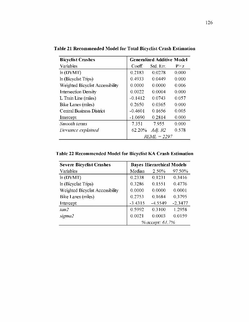
126
Table 21 Recommended Model for Total Bicyclist Crash Estimation
Bicyclist Crashes Generalized Additive ModelVariables Coeff. Std. Err. P>|z|ln (DVMT) 0.2183 0.0278 0.000ln (Bicyclist Trips) 0.4933 0.0449 0.000Weighted Bicyclist Accessibility 0.0000 0.0000 0.006Intersection Density 0.0022 0.0004 0.000L Train Line (miles) -0.1412 0.0743 0.057Bike Lanes (miles) 0.2650 0.0365 0.000Central Business District -0.4601 0.1656 0.005Intercept -1.0690 0.2814 0.000Smooth terms 7.351 7.955 0.000Deviance explained 62.20% Adj. R2 0.578
REML = 2297
Table 22 Recommended Model for Bicyclist KA Crash Estimation
Severe Bicyclist Crashes Bayes Hierarchical ModelsVariables Median 2.50% 97.50%ln (DVMT) 0.2338 0.1231 0.3416ln (Bicyclist Trips) 0.3286 0.1551 0.4776Weighted Bicyclist Accessibility 0.0000 0.0000 0.0001Bike Lanes (miles) 0.2753 0.1684 0.3795Intercept -3.4315 -4.5549 -2.3477tau2 0.5992 0.3100 1.2958sigma2 0.0021 0.0003 0.0159
% accept: 61. 7%

Figure 23 presents the relationship between DVMT and the estimated vehicular crash
rate for total and severe vehicular crashes, in the case when all other variables for these
particular models are kept constant. Figure 24 presents the relationship between the
exposure variables considered in the pedestrian crash models, including the DVMT and
the estimated generated pedestrian trips. The effects of the variables that resulted from
the multimodal accessibility analysis and were found to be associated with total and
severe pedestrian crashes are provided in Figures 25 and 26. Figure 26 presents the
relationship between the exposure variables in the bicyclist crash models that include
DVMT and estimated generated bicyclist trips, and total and severe bicyclist crash
outcome. Figure 27 presents the effects of bicyclist accessibility on total and severe
bicyclist crashes.
These results presented in Figures 23 through 28 are extracted to support the further
interpretation of the results provided in the finally recommended models that are
provided in Tables 17 through 22. The estimated coefficient values and signs in the final
model recommendations mostly show that the increase in exposure or accessibility is
associated with the increase in crashes for different modes, but a more detailed
representation of results shows nonlinear relationships between these variables and crash
outcomes. The interpretation of the effects presented in Figures 23 through 27 is provided
in the following Discussion chapter.
127

128
Relationship between Total Vehicular Crash Rate and DVMT
p 0.500
>Qfe 0.400Q.jr/, n nnu.^uu
1u
£ °-200
£ 0.100
0.000
)050 100 150 2(
DVMT
0.016
0.014P
Relationship between Severe Vehicular Crash Rate and DVMT
%\XU.UIZQS_
3 0.010
iiv n nns
\\%\\\\U .U U o
1r*r n rin/z
\\\VO U.VJUO
jH n DDA
X N
' no u.uu +
:>0.002
0.0000 50 100 150 200
DVMT
Figure 23 The “Safety in Numbers” Effect for Private Vehicle Users

Ped
est
rian
Cra
sh
Rat
e (p
er
pedest
rian
tr
ips)
Pedest
rian
Cra
sh
Rat
e (p
er
DV
MT
)
129
Relationship between Pedestrian Crash Rate and DVMT
0.250
0.200
0.150
0.100
0.050
0.000
—•— Total Pedestrian Crashes
-♦ -SeverePedestrian Crashes
50 100DVMT
150 200
R elationship betw een Pedestrian Crash Rate and Pedestrian Trips
0.450
0.400
0.350
0.300
0.250
0.200
0.150
0.100
0.050
0.00050 100
Pedestrian Trips
150 200
Figure 24 The “Safety in Numbers” Effect for Pedestrian Users

Pede
strian
Cr
ash
Rate
(per
pede
stria
n tri
ps)
Pede
strian
Cr
ash
Rate
(per
pede
stria
n tri
ps)
Pede
strian
Cr
ash
Rate
(per
pede
stria
n tri
ps)
130
Relationship between Pedestrian Crash Rate and Weighted Pedestrian Accessibility
0.450
0.400
0.350
0.300
0.250
0.200
0.150
0.100
0.050
0.000
----- Ped_A=0.05
----- Ped_A=0.25
-----Ped_A=0.50
— Ped A=0.75
----- Ped_A=l .00
50 100Pedestrian Trips
150 200
Relationship between Pedestrian Crash Rate and Cumulative Pedestrian Accessibility
Pedestrian Trips
-Ped_D15=10 ----- Ped_D15=25 ----- Ped_D15=50 — Ped_D15=75 ----- Ped_D15=100
Relationship between Pedestrian Crash Rate and Transit Accessibility
-Transit A=10 -Transit A=25
Pedestrian Trips
-Transit A=50 -Transit A=75 -Transit A=100
Figure 25 Relationship Between Total Pedestrian Crashes and AccessibilityVariables

Ped
estr
ian
Cra
sh
Rate
(p
er pe
dest
rian
tr
ips)
Ped
estr
ian
Cra
sh
Rate
(p
er pe
dest
rian
tr
ips)
131
Relationship between Severe Pedestrian Crash Rate and Weighted Pedestrian Accessibility
Pedestrian Trips
Relationship between Severe Pedestrian Crash Rate and Cumulative Pedestrian Accessibility
Pedestrian Trips
---Ped_D15=10 ---PedD 15=25 --- Ped_D15=50 ---Ped_D15=75 --- Ped_D15=100
Figure 26 Relationship Between Severe Pedestrian Crashes and AccessibilityVariables

Bic
yclist
Cra
sh
Rate
(p
er
bic
yclistt
rips)
Bic
yclist
Cra
sh
Rate
(p
er
DV
MT
)
132
Relationship between Bicyclist Crash Rate and DVMT
DVMT
Figure 27 The “Safety in Numbers” Effect for Bicyclist Users

Bic
yclis
t Cr
ash
Rate
(per
bic
yclis
ttrip
s)
Bic
yclis
t Cr
ash
Rate
(per
bi
cycl
isttr
ips)
133
Relationship between Bicyclist Crash Rate and Weighted Bicyclist Accessibility
0.120
0.100
0.080
0.060
0.040
0.020
0.000
----- Bike_A=0.01
----- Bike_A=0.10
Bike_A=0.25
Jj IKC A U.j U
----- Bike_A=0.75
50 100Bicyclist Trips
150 200
Relationship between Severe Bicyclist Crash Rate and Weighted Bicyclist Accessibility
0.008
0.007
0.006
0.005
0.004
0.003
0.002
0.001
0.000
-----Bike_A=0.01
-----Bike_A=0.10------ R iVp A = n 75O I a C r \ U . l i J
Bike_A=0.50
-----Bike_A=0.75
50 100Bicyclist Trips
150 200
Figure 28 Relationship Between Bicyclist Crashes and Accessibility Variables

CHAPTER 5
DISCUSSION OF STATISTICAL AREAL SAFETY
MODELING RESULTS
This chapter presents the discussion of the SASM modeling results that are provided
in the previous chapter. For each crash type, this chapter discusses all the variables that
were associated with the expected number of crashes. Models are interpreted starting
with the preliminary modeling specifications, to the final modeling specifications that
were interpreted in detail. The SASM diagnostics provided in the previous chapter and
the estimated final model specifications were used to explain how the final model
recommendation was made. The end of this chapter provides the interpretation of the
“Safety in Numbers” effect and the potential role of using accessibility measures to
model multimodal safety outcomes.
Preliminary Model Specifications
Initial SASM analysis was based solely on the negative binomial models for all six
crash types that were analyzed in this research. The preliminary models for each crash
type were run iteratively using different groups of variables provided in the Data chapter,
as the number of variables did not allow the inclusion of all variables into a single model,
particularly considering that the dataset consisted of roughly 100 variables for 801
observations/census tracts.

In order to obtain the preliminary set of potentially relevant variables that were further
considered for the final model specifications, the variable selection was carried out using
the approach described in the Methodology chapter. The groups of variables that proved
to be potential candidates for the final model specifications for all crash types included
variables related to demographics, exposure, accessibility, intersections and traffic
control, multimodal infrastructure, land use, street connectivity, and network
completeness. Variables that were excluded after the preliminary modeling process
included economic characteristics, commuter trips to work by mode, and the majority of
variables representing functional classification of the street network.
Final Model Specifications
Tables 10 through 15 present the final model specifications for each response variable
by SASM method applied. This section provides a detailed discussion of the effects of
each variable included in final model specifications by crash type.
Total Vehicular Crashes
The statistical modeling results for total vehicular crashes are provided in Table 10,
for all modeling approaches applied to the dataset. The final model specification for
vehicle crash frequency includes population density, total miles of road, DVMT,
intersection density, percent of signalized intersections, bus stops, and sidewalk area.
The results indicate that the expected crash frequency increases as population density
increases, and similar findings have been reported in the literature (Castro et al., 2013;
Flask & Schneider, 2013; Noland & Quddus, 2004). Other socio-economic variables did
not show significant effects on the expected frequency of vehicular crashes. This could be
due to the level of mobility of vehicular traffic, as vehicular trips can be generated
135

through the census tract areas regardless of economic status of the population. The
natural logarithm of road mileage and DVMT were used as the exposure variables to
estimate the expected number of vehicular crashes on the census tract level. Although
DVMT is calculated from the ADT values related to each link in census tract multiplied
by the length of corresponding links, thus incorporating road segments length into this
measure, total road mileage is still included in vehicular crash models. Under the
assumption that the dataset includes two census tracts with the same DVMT, one of these
census tracts could have a denser road network and higher road mileage with lower
volumes of traffic, while the other census tract could have fewer roads but higher traffic
volumes resulting with the same DVMT value. It is expected that these two hypothetical
census tract areas would have different number of vehicular crashes, even though their
DVMT value is the same, due to differences in the road network structure, and traffic
flow intensity and its distribution across the network. This is why road mileage variable
is included as an additional exposure variable in vehicular crash models.
As expected, increases in total length of roads in miles and daily vehicle miles traveled
were associated with an increase in expected crash frequency at the 99 % confidence
level. Comparing the two measures of exposure, and their effect on the expected number
of crashes, the length of roads contributes to the increase in the expected number of
vehicular crashes more than the value of DVMT. If road mileage on the census tract level
was doubled, according to the estimated models for total vehicle-only crashes, the
expected number of crashes is expected to almost double. The impact of DVMT cannot
be interpreted in the same manner, as the estimated model shows that if DVMT on a
census tract level doubles, crashes are expected to increase by less than 20 %.
136

Intersection-related variables, such as intersection density and the percentage of
signalized intersections, were associated with expected crash frequency on census tract
level, where increases in these variables were associated with increases in crashes.
Intersections are considered to be major points of conflict, which could be the reason for
the positive sign of the coefficients estimated for these variables. Previous studies have
found some similar relationships between network and intersection densities and crash
frequencies (Moeinaddini, 2014; Siddiqui, 2012). The estimated coefficients show that
the increase in the share of signalized intersections contributes to associated increase in
the expected number of crashes up to fifteen times more than the same change in the
overall number of intersections per mile squared. The presence of traffic signals may be
increasing certain types of crashes (e.g., rear-end crashes), which may be the reason for
the positive parameter sign and significance of this variable in the models.
The presence of L Train lines in Chicago is usually associated with environments
where multimodal transportation is encouraged, with more people walking, biking, or
taking transit. Particularly, the areas around L Train stops in downtown are designed to
discourage higher vehicle speeds, and perhaps even reduce the number of people driving.
During the preliminary modeling process, the presence of L Train lines was statistically
significant variable in the models, with the negative sign of the coefficient. The
significance of the variable and the magnitude of the estimated coefficients, however,
varied between different statistical models, so the variable was not included in the final
model specification.
Presence of bus stops was associated with an increase in expected vehicle crash
frequency. There are usually the areas where vehicles may be forced to change their
137
speeds, which could lead to higher number of conflicts, and higher crash frequency. The
increase in the number of bus stops by 1 % is estimated to contribute to 0.3 % increase in
the expected number of vehicular crashes.
The total area of sidewalk was associated with decrease in vehicular crash frequency,
where the addition of 500 feet squared of sidewalk could reduce the expected number of
crashes by up to 2 %. This impact, however, is not as strong as the estimated impact of
some previously discussed variables that are associated with the increase in crashes.
Previous studies mostly relate this variable to nonmotorized crash frequency (Wang &
Kockelman, 2013). In urban environments, presence of sidewalk and other features
related to walkability may be a characteristic of areas where people drive less, or drive
more cautiously, thus leading to lower number of vehicular crashes.
Severe Vehicular Crashes
Table 11 provides the results of the estimated statistical models for the frequency of
severe vehicular crashes. The variables that are found to be associated with the expected
number of severe vehicular crashes include road mileage, DVMT, percent of signalized
intersections, bus stops, sidewalk area, L train stops, and land use entropy.
To account for the difference between census tracts with the same DVMT values, but
different road network mileage, both road mileage and DVMT were used as the exposure
variables in the estimated models for severe vehicular crashes. Similar to total vehicular
crashes, the estimated model results show that it can be expected that the number of
crashes follows the rate of change of road segment lengths, while the increase in traffic
volumes is not followed by the proportional increase in crashes.
138

The results from the estimated severe vehicular crash models also show that if the
share of signalized intersections in census tracts is increased by 1 %, the expected
increase in severe vehicular crashes would be 1.39%. The presence of traffic signals
contributes to increase in both total and severe vehicular crashes. The effect of this
variable on crash frequency and severity implies that some additional research that would
consider crash types (e.g., rear-end, angle crashes) would be beneficial when it comes to
exploring urban safety. The impact of the presence of signals on the increase of
frequency and severity of intersection related crashes is already proven in previous
research and recognized in intersection crash predictive methods.
Presence of sidewalk was associated with the decrease in severe vehicular crashes.
The estimated results show that the addition of 500 feet squared of sidewalk would result
in 1.29% reduction in severe vehicular crashes. The results from the estimated models for
total vehicular and sever vehicular crashes indicate that sidewalk could be considered as a
safety countermeasure in urban environments. The limitation that should be considered
here is that very few cities would have the available data on sidewalk area coverage, so
some approximations should be considered in order to use the model in different
locations.
Just as in the case of the models developed for total vehicular crashes, the number of
bus stops within the census tract was associated with the increase, while the number of L
Train stops was associated with the reduction in the severe vehicular crashes. One percent
increase in the number of bus stops is expected to lead to less than 0.2 % increase in
severe vehicular crashes. The expected reduction of severe vehicular crashes with the
addition of L Train stops (1 % increase in numbers) is lower than 0.1 %. The opposite
139

signs of the effects of L Train facilities which are grade separated, and bus stops which
are mostly alongside the lanes shared by both private vehicles and buses, indicate the
potential benefits from investing in prioritizing transit and separating it from the rest of
the traffic flow whenever possible.
The increase in land use mix expressed as entropy measure on a scale from zero
(single land use) to one (all land uses) showed association with the increase of the
number of severe crashes. This association is not very strong, as 1 % increase in entropy
would result to 0.35% increase in the expected number of severe vehicular crashes. The
influence of mixed land use on the expected number of crashes is explored in some
previous studies, mostly related to pedestrian crashes. The possible explanation for the
effect of land use mix on the increase on severe vehicular crashes is the diversity of land
use mix characteristics that exists among census tracts in Chicago, ranging from
predominantly single-use to very high land use mix areas, where the majority of trips,
particularly work commute trips, are directed towards destinations in high land use mix
parts of the city such as downtown. This variable is eventually excluded from the final
model recommendation for the severe vehicular crashes due to inconsistent values of the
estimated coefficients as well as lack of logical explanation for the interpretation of the
relationship. However, the potential impact of entropy could be important to consider in
order to distinguish between different aspects of urban environment, rather than just
adopting the same effects on safety outcome for urban roads and networks in general, or
simply categorizing area-wide effects as urban and suburban.
140

The estimated statistical models for the expected number of total pedestrian crashes in
census tracts are provided in Table 12. The variables that were associated with the
expected number of pedestrian crashes include DVMT, the number of pedestrian trips
within the census tract, weighted pedestrian accessibility, the number of destinations
accessible within 15-minute walking time, average daily transit accessibility, percentage
of arterials, intersection density, percent of signalized intersections, street connectivity,
sidewalk area, and the percent of network with complete streets.
The expected pedestrian crash outcome depends on both DVMT and the number of
pedestrian trips. Based on the results provided in Table 12, 1 % increase in the expected
pedestrian crashes would result from 5 % increase in pedestrian trips, if all other
variables remain unchanged. The same increase of 1 % in pedestrian crashes is also
expected to occur if the value of DVMT increases by 15 %. This gives the impression
that the presence of pedestrians contributes to the increase in pedestrian crashes. The
estimated coefficients for the exposure variables, however, indicate that the expected
number of crashes does not increase proportionally with the increase in vehicular or
pedestrian trips, and this effect will be discussed in the last section of this chapter.
The accessibility indicators were used in the estimated statistical models as the
additional variables that could indicate pedestrian activity within and between the census
tracts. The accessibility indicators that were found to have statistically significant impact
on the pedestrian crash outcome primarily refer to the ability of pedestrians whose trips
origins are within census tracts to reach destinations by walking or transit. Pedestrian
crashes are expected to increase as the pedestrian accessibility increases as a function of
the number of accessible destinations and travel time to destinations. This relationship
141
Total Pedestrian Crashes

between the number of the accessible destinations and the travel time for pedestrians
depends on the land use patterns and the street network structure. The increase in
weighted accessibility could occur due to the increase in the number of opportunities
within the given travel time, or due to the decrease in the travel time needed to reach the
opportunities. The total number of destinations that pedestrians are able to reach within
the 15-minute walk is associated with decrease in pedestrian crashes. These two variables
have different signs, indicating that the concentration of opportunities in such a way that
it decreases the length of pedestrian travel time could lead to pedestrian crash reduction.
The reasoning behind this could be that shorter pedestrian trips to destinations, and
developing land use patterns and transportation structuring networks in a way that
enables pedestrians to reach the opportunities within shorter amount of time, could
influence the reduction of their exposure to conflicts and as a result of that the reduction
of crashes. As the number of pedestrian destinations outside of the 15-minute threshold
increases, their weight will decrease but the overall accessibility can still gradually
increase, and influence the creation of longer pedestrian trips and thus more opportunity
to be exposed to crashes. One percent increase in the average daily transit accessibility is
estimated to lead to 0.9% increase in the expected number of pedestrian crashes. The
statistical significance of accessibility indicators in the estimated pedestrian crash models
implies that these indicators could serve to provide additional information about
pedestrian exposure to crashes in urban environments, particularly when estimating the
expected number of crashes on a larger scale.
Variables that represent functional classification, street network connectedness,
conflict points, and intersection traffic control are associated with the increase in
142

pedestrian crashes. If the presence of arterials on the street network were to increase by 1
%, it is expected that the frequency of pedestrian crashes would increase by 0.1 %. If the
intersection density was increased in the similar way, it is estimated that it would have a
slightly stronger effect on pedestrian crashes that are expected to increase by 0.2 %.
Intersection density represents the number of intersections per mile squared of census
tract area, while street connectivity is a better indicator of street network connectedness
as is it obtained by dividing the number of nodes by the actual miles of road in the census
tract. Street connectivity is associated with the reduction of pedestrian crashes, implying
that two census tracts with the same intersection density may differ in terms of the
expected number of pedestrian crashes if one of them has higher number of four-leg
intersections, as according to the results census tracts with more three-leg intersections
are expected to have lower pedestrian crash frequency. The presence of signalized
intersections is associated with the expected number of pedestrian crashes, and appears to
be the major driver of pedestrian crash occurrence among the variables in the pedestrian
crash model. According to the estimated model, pedestrian crashes are expected to
increase by 1.16 % in census tracts with the 1 % increase in signalized intersections. The
estimated impact of signalized intersections on pedestrian crashes is expected as
signalized intersections can be identified as the network locations with the major
potential for vehicle-pedestrian conflicts. Similar effects of the presence of signalized
intersections on pedestrian crashes were reported in previous research (Ukkusuri et al.,
2012).
The key for determining the final model specification for estimating pedestrian crash
outcome was to select the adequate measures of exposure to capture the opportunities for
143
pedestrian crashes to occur within census tracts. The product of DVMT and the number
of pedestrian trips within census tract estimated from the CMAP trip generation model
served as the main indicator of pedestrian exposure to crashes. It was assumed that if
either of these two variables (DVMT or the number of pedestrian trips) is equal to zero,
no pedestrian crashes would be expected. Additional measures that would serve as a
proxy for exposure were considered during the statistical modeling process, including the
total road mileage and sidewalk area. In the case where roadway mileage was included in
the models, sidewalk area was treated as a form of pedestrian safety countermeasure and
the statistical modeling results would show sidewalk as associated with crash reduction.
In the case where roadway mileage was excluded from the models, sidewalk served as
the approximation for roadway facilities with pedestrian presence, and was associated
with the increase in pedestrian crashes. A better, more complete measure that indicates
pedestrian presence on roadway facilities, particularly in the context of the potential
conflicts between multimodal users, was the indicator of network completeness,
expressed as the percentage of network that serves all four modes. The estimated model
results show that if the percentage of street network that serves all four modes is
increased by 1 %, the expected increase in pedestrian crashes would be 0.39 %. Statistical
models that serve to estimate pedestrian crash outcome, particularly on the areal level,
should include some indicators related to pedestrian infrastructure that would
complement the measures of exposure. Whether simply road mileage, or sidewalk area,
or in this case, an indicator of the presence of complete streets in the network is used, will
depend primarily on the data availability and the complexity of multimodal networks.
144

Some other variables were also considered and included in the preliminary model
specifications for pedestrian crashes, such as the population density and the percentage of
unemployment in census tracts. Both of these variables were associated with the increase
in the expected number of pedestrian crashes. The presence of L Train lines and stops
was associated with the reduction of pedestrian crashes during the statistical modeling
process, while bus routes appeared to be associated with the increase in pedestrian
crashes. Some of these findings were expected. For example, it is more likely that people
would walk in lower-income neighborhoods, which may be the reason why the
percentage of unemployment showed some association with the increase in pedestrian
crashes. The areas around L Train lines are usually highly walkable areas, where
vehicular speeds tend to be lower despite the fact that trains are grade-separated. This
explains the negative coefficient sign which indicated the association of the presence of L
Train lines with a decrease in pedestrian crashes. Increases in the number of bus routes
were also associated with increases in the expected number of pedestrian crashes, as
pedestrian protection islands and similar measures are not too frequent along the bus
routes, especially in higher density and mixed land use areas. These several variables
were not included in the final model specification for total pedestrian crashes, as they did
not remain statistically significant through the statistical modeling process, and some of
them were unique to the City of Chicago and would be difficult to implement if similar
models were to be developed for other urban environments.
Severe Pedestrian Crashes
The estimated statistical models for the expected number of severe pedestrian crashes
in census tracts are provided in Table 13. The variables that were associated with the
145

expected number of severe pedestrian crashes include DVMT, the number of pedestrian
trips within the census tract, weighted pedestrian accessibility, the number of destinations
accessible within 15-minute walking time, and the percent of signalized intersections.
For the relevant measures of exposure for severe pedestrian crashes, the same
approach was used as in the case of estimating total pedestrian crashes. The estimated
DVMT and the number of pedestrian trips were used as the measures of exposure.
Statistical models for severe pedestrian crashes are setup in such a way that if one of
these two variables (either DVMT or the number of pedestrian trips) in a particular
census tract is zero, it is assumed that no pedestrian crashes are expected to occur in that
census tract. According to the results presented in Table 13, if DVMT within the census
tract increases by 1 %, the expected increase in severe pedestrian crashes is estimated to
be 0.2 %. The same 1 % increase in the number of generated pedestrian trips on the
census tract level is expected to contribute to 0.39 % increase in severe pedestrian
crashes. While the increase in pedestrian trips seems to have a stronger influence on the
expected severe pedestrian crash outcome then the increase in DVMT, the expected
increase in severe pedestrian crashes is not proportional to the increase in DVMT and
pedestrian trips.
While weighted pedestrian accessibility shows association with the increase in severe
pedestrian crashes, the number of destinations accessible within 15-minute walking time
are associated with crash reduction. The 1 % increase in overall pedestrian accessibility
may be contributing to up to 0.5 % of increase in severe pedestrian crashes. The
estimated effects of the 15-minute cumulative pedestrian accessibility measure are less
strong, as the number of destinations accessible by walking needs to be more than
146

doubled in order to expect measurable crash reduction. Cumulative measures are
capturing spatial distribution of activity points and pedestrian network robustness, while
weighted accessibility is more representative of the travel efficiency expressed through
travel time. These results indicate that while pedestrians are safer in environments where
there are more opportunities to reach diverse destinations, more efficient trips are not
always expected to be safer.
Just as in the case of total pedestrian crash model, the major driver of severe
pedestrian crashes seems to be the percent of signalized intersections within the census
tract. According to the results from the Table 13, if the number of signalized intersections
within census tracts was increased by 1 %, severe pedestrian crashes would increase by
0.8 %. These results indicate that signalized intersections are associated with higher
concentrations of total and severe pedestrian crashes, which could be an implication for
future city-wide pedestrian safety investments.
Some other variables that showed association with the increase in severe pedestrian
crashes included population density, intersection density, the number of bus stops, the
number of bike racks, transit work trips, and land use diversity. Census tract sidewalk
area showed association with the reduction of severe pedestrian crashes during the
statistical modeling process included. The majority of these variables were similar to
those included in the model specification for total pedestrian crash estimation. This is
expected, as variables such as the intersection density or the number of bus stops relate to
the number of conflicts to which pedestrians are exposed. An additional explanation
could be that if a pedestrian is in a crash, it is more likely that the pedestrian will be
severely injured when compared to, for example, vehicle occupants. These variables
147

varied in terms of their effect on severe pedestrian crashes as well as statistical
significance in the models, and were excluded from the final model specification.
Total Bicyclist Crashes
The estimated statistical models for the expected number of bicyclist crashes in census
tracts are provided in Table 14. The variables that were associated with the expected
number of bicyclist crashes include the estimated DVMT, the number of bike trips within
the census tract, weighted bicyclist accessibility, intersection density, bus stops, bike
lanes mileage, CBD, and the presence of L Train lines.
The estimated DVMT and the number of generated bike trips were used as the primary
measures of exposure. The estimated coefficients for volumes of vehicles and bicyclist
trips in census tracts show nonlinear relationship with the bicyclist crash outcome.
Similar to pedestrian crashes, the expected number of bicyclist crashes is increasing at a
significantly lower rate when compared to the increase in vehicular and bicyclist volume
rates. It is estimated that it would take a 6 % increase in DVMT, or the alternative 3 %
increase in the number of biking trips, to expect a 1 % increase in bicyclist crashes.
Bike lanes mileage, the weighted bicyclist accessibility, and the intersection density
were used as the approximate measures of the opportunities for conflicts between
bicyclists and vehicles. While in the case of vehicular crashes where doubling the road
length would be expected to result in almost double number of crashes, the same
conclusion cannot be drawn for the bicyclist crashes and bike lanes where doubling the
mileage of bike lanes is not expected to be followed by the same increase in bicyclist
crashes (bicyclist crashes are expected to increase by 24% rather than double). This is
148

probably due to the fact that biking may also be present on the road segments that do not
include bike lanes.
Weighted bicyclist accessibility is the indicator of the potential biking activities in the
city, and is included in the model as a statistically significant variable. The estimated
impact on crash outcome, however, is very small, as 1 % increase in bicyclist
accessibility is estimated to result in 0.02% increase in bicyclist crashes. This effect is
much less significant than the effect that pedestrian and transit accessibility indicators
were estimated to have on pedestrian crashes. The overall destination accessibility is
always higher for bicyclists than for pedestrians, and pedestrian mode is more sensitive to
the way street network is integrated with land use patterns, which may be the cause of the
estimated results. In addition, bicyclists are not always expected to use only biking
infrastructure, while pedestrians movements are usually expected to be closely related to
pedestrian facilities which influence the accessibility indicators and could potentially
influence the exposure to crashes.
Intersection density proved to be statistically significant variable in the total bicyclist
crashes model specification. While the presence of traffic signals was the major driver of
vehicular and pedestrian crashes, the density of intersections appears to be more relevant
for the expected number of bicyclist crashes. Pedestrians are mostly exposed to crashes at
particular points along the roadway segments (pedestrian or mid-block crossings), where
the exposure increases with the volumes of vehicles that are higher at signalized
intersections. Bicyclists are more exposed to crashes than pedestrians in terms of spatial
opportunities for conflicts, as the conflicts may occur anywhere along the roadway
segments, which may be the reason why the type of intersection traffic control is less
149

significant. The effect of intersection traffic control on bicyclist crashes on a smaller
scale should be further explored.
The CBD area, presence of bus stops, and the presence of L Train facilities served as
additional area-wide effects that proved to have significant influence on the expected
number of bicyclist crashes. The downtown area in Chicago tends to be more oriented
towards nonmotorized modes, with better defined biking facilities network. However,
additional analysis is needed to determine if different types of biking facilities (e.g.,
protected bike lanes), tend to lead to reduction of biking crashes. Biking trips do have
higher concentrations in the downtown area, and given the estimated coefficient that
indicates that bicyclist crashes are less likely to occur in CBD area, this could confirm the
nonlinear relationship between the number of people biking and bicyclist crash outcome.
The estimated model results (Table 14) show that 1 % increase in bicyclist crashes is
expected to occur if the number of bus stops in census tracts is increased by 2 %. The bus
stops routes in Chicago rarely have dedicated lanes, and the bus stops are typical speed-
changing areas due to bus traffic lane-changing and interfering with vehicular traffic.
These types of interactions may be causing conflicts with bicyclists as well, especially
because bike racks are usually located near the bus stations. Bike racks have appeared as
a statistically significant variable during the statistical modeling process, but were
excluded from the final model specification as they did not show stable effect through the
iterative modeling process, and they showed smaller effect when compared to other
variables included in total bicyclist crashes specification. This probably occurred due to
the fact that the presence of bike racks is captured through other variables such as bike
150

lanes or CBD. This, however, could be a promising variable to explore, particularly when
exploring bicyclist crashes on a larger scale in the future.
The L Train facilities showed association with bicyclist crash reduction. The addition
of 1 mile of train facilities is estimated to result in 13 % reduction in bicycle crashes. It is
important to acknowledge here that the crash reduction may not be the result of the
presence of train facilities, but the environment that is created due to the particular design
of train line and station facilities, particularly in Chicago. In this case, having the elevated
rail structures is very often followed by lower driving speed, more walking and biking,
which could be the reason of association of L Train presence with the bicyclist crash
reduction.
Among other variables, socio-economic variables do not appear to have statistically
significant effects on crashes involving bicyclists. The effects of entropy and land uses
were also explored, and did not show stable association with bicyclist crash outcome.
Severe Bicyclist Crashes
The estimated statistical models for the expected number of severe bicyclist crashes in
census tracts are provided in Table 15. The variables that were associated with the
expected number of severe bicyclist crashes include the estimated DVMT, the number of
bike trips within the census tract, weighted bicyclist accessibility, and bike lanes mileage.
All variables that were statistically significant in the estimated severe bicyclist crash
model were already included in the total bicyclist crashes model specification. The same
exposure variables, the estimated DVMT and bicycle trips within the census tracts, were
used to estimate the expected number of severe bicyclist crashes. These variables are
estimated to have a nonlinear relationship with the expected number of severe bicyclist
151

crashes, where a percent increase in bicycle trips or DVMT is followed by 0.2% to 0.25%
increase in bicyclist crashes.
Bicyclist accessibility is included in the estimated model for severe bicyclist crashes,
as a statistically significant variable. However, the effect is very small, similar to the
effect present in the case of total bicyclist crashes. Unlike the pedestrian crashes, bicyclist
crashes are less dependent on accessibility-related variables. As the ability to reach
destinations by bike is much higher than the ability to reach destinations by walking,
bicyclist accessibility (cumulative or weighted) did not show statistically significant
impact on bicyclist crash frequency or severity.
Another predictor that was found to have a significant effect on the severe bicyclist
crashes is the total length of bike lanes within census tracts. Severe bicyclist crashes are
expected to increase in census tracts that have higher mileage of bike lanes, but not at the
same rate at which the bike lane length increases.
Some other variables, including the sidewalk area and the land use entropy, showed
some impact on the severe bicyclist crashes, but the direction of impact did not seem
logical (e.g., increase in sidewalk area was associated with the increase in bicyclist
crashes), and these variables were not included in the final model specification.
Diagnostics and Final Model Recommendations
The final model recommendation for each crash type depended on the comparison of
final model specifications estimated by using the applied SASM methods, the model-
specific goodness of fit indicators provided in Tables 10 through 15, and the model
diagnostics provided in Table 16.
152

Based on the results provided in Tables 10 through 15, the SASM approaches applied
in this research were fairly consistent in terms of the variables that were influential and
statistically significant in each crash model. Negative binomial models, although not able
to capture spatial spillover effects, provided a strong indication about the variables that
should be considered when modeling various types of crashes in urban multimodal
environments. However, using only negative binomial models, without running other
statistical models, would not lead to adequate final model specifications, as the
application of different SASM methods helped to eliminate the variables with
inconsistent signs and estimated coefficient values. Running different types of models
with same sets of variables is what helped to determine first the final model specification,
and then the best model recommended for the estimation of each crash type in the
analysis.
As the data were spatially collected, accounting for spatial auto-correlation and
generally spatial relationships between census tracts was an important part of SASM
process. The first step to account for spatial effects in the data by simply assuming that
larger spatial entities such as Planning Districts and Regions can capture spatial
dependence between census tracts. This approach was modeled by incorporating fixed
and then random effects into negative binomial models. Regions proved to be statistically
significant in negative binomial models with fixed effects for all crash types. Looking at
the model diagnostics presented in Table 16, models with fixed effects also outperformed
negative binomial models with random effects, but further steps needed to be taken to
ensure that the impact of certain variables is not overestimated due to spatial
autocorrelation present in crash data for all users. This is why generalized additive
153

models with smooth functions across the locations were used, as an alternative frequentist
approach that has the ability to fit spatially collected data. When compared to negative
binomial models, GAM showed that the smooth terms included in the model to represent
spatial trends in the data were significant at the 99% confidence level for total and severe
vehicular, pedestrian, and bicyclist crashes. The inclusion of smooth functions to account
for spatial autocorrelation resulted in slightly higher standard errors and lower statistical
significance levels for some variables in the models. For example, the presence of bus
stops appears to be less significant in terms of its effects on vehicular crashes when
modeled with spatial trend functions in GAM approach compared to other frequentist
methods. Similar trends occur with land use entropy in severe vehicular crash models,
with L Train lines in total bike crash models, and weighted bicyclist accessibility in
severe bike crash models. The percent of deviance explained by the models is the highest
for the total vehicular crash models (76.30%), and slightly lower for total bicyclist
(62.20%) and total pedestrian crash models (43.70%). While the model for severe
vehicular crashes has relatively high percent of deviance explained by using the
generalized additive models (63.20%), the scores are significantly lower for severe
bicyclist crashes (31.70%), and severe pedestrian crashes (20.80%).
The clear advantage of FBH models presented in Tables 10 through 15, over
frequentist modeling approaches, is the estimation of two sets of random effects: one
resulting from spatial correlation, and the other from unobserved heterogeneity among
census tracts. The set of statistically significant variables is almost the same for Bayesian
models when compared to negative binomial and GAM. The variables that are marginally
significant in negative binomial models are not significant in the Bayesian hierarchical
154

models, similar to GAM results. The variance due to spatial correlation estimated in
Bayesian models is low but different from zero, confirming the findings from the GAM
approach that spatial correlation is statistically significant.
Table 16 shows the model diagnostics for vehicle, pedestrian, and bicyclist crash
models. The values of AIC and BIC were used for frequentist approaches, while DIC was
used for FBH models. The DIC and BIC values provided in Table 16 were the lowest for
GAM models among all frequentist models, indicating that GAM models are a more
efficient approach than other explored frequentist SASM methods to represent the data
generating process for different crash types. When comparing the AIC and BIC values for
the methods based on frequentist statistical inference, GAM outperform linear forms of
negative binomial model, including the models with fixed and random effects. While
direct comparison of the statistical models based on frequentist and Bayesian approach
cannot be made, the models can be compared in terms of the coefficients and the overall
efficiency of executing the modeling process. It is well known that the major
disadvantage of FBH modeling process is that it may be more time consuming and
challenging in terms of the coefficient interpretation, as it provides the results in the form
of a distribution rather than p-values and confidence intervals.
The results of the obtained models show very similar coefficient values for GAM and
FBH models, with a relatively high percent of deviance explained by the GAM in the
case of the models used to estimate total crash frequency for different modes of
transportation. Similar conclusion can be made about the GAM models used to estimate
severe vehicular crashes. The percentage of deviance explained and the similarity in the
coefficients resulting from GAM and FBH estimation led to the selection of GAM
155

approach as the recommended approach for vehicular (total and severe), total pedestrian,
and total bicyclist crash estimation. In the case of these four crash types, the spatial auto
correlation is lower than in the case of severe nonmotorized crashes, and there are not too
many census tracts with zero crash outcomes, meaning that the application of FBH would
not significantly contribute in terms of treating these data issues. This is why GAM
approach, which also outperforms other frequentist approaches in terms of diagnostics
values and estimated coefficient standard errors, is selected as a valid SASM alternative
to estimate these crash types.
In the case of severe pedestrian and severe bicyclist crashes, spatial auto-correlation is
slightly higher than for the other analyzed crash types. The number of census tracts with
zero crash outcomes is also higher for these two crash types. The FBH models have been
known to handle the excessive number of zero observations in crash datasets, as the
approach is based on MCMC simulation which allows more flexibility in terms of
sampling values from the posterior distribution without actually declaring zero-state as a
fixed state for any of the observations. This is why in the case of severe pedestrian and
bicyclist crashes, FBH models were recommended as the most suitable.
Safety Effects of Multimodal Exposure and Accessibility
In addition to interpreting the variables that were included in the final model
recommendations for each crash type, the variables related to multimodal exposure and
accessibility were extracted and their effects on multimodal safety outcomes were
separately presented in Figures 23 through 28. The estimated models for total and severe
vehicular, pedestrian, and bicyclist crashes show that the increase in crashes for all crash
types is associated with the increase in the majority of variables representing multimodal
156

infrastructure, exposure, or accessibility. This section of the Discussion chapter is
intended to clarify these relationships by taking a more detailed look into the effects of
exposure and accessibility on multimodal safety outcomes.
Figures 23, 24, and 26 show the relationships between the exposure variables and
associated crash rates for total and severe crashes. As previously explained, non
motorized crashes were estimated using the combinations of exposure measures for
private vehicles (DVMT) and the adequate nonmotorized mode (pedestrian trips or
bicyclist trips). The relationships between crash rates for all crash types and the related
exposure measures are nonlinear. The estimated coefficients for the exposure variables in
all estimated models have a value lower than one. This means that while the crashes are
expected to increase as the exposure increases, the increase in crash rate is expected to be
much lower than the rate at which the exposure increases, and this can be concluded for
crash outcomes for all crash types. This effect where crashes increase at a lower rate (rate
that is not proportional to exposure rate) than the exposure is known in the literature as
the “Safety in Numbers” effect (Elvik, 2015; Hauer, 1982).
As the exposure increases for private vehicle users, total vehicular crashes are
expected to increase at a much higher rate than the severe vehicular crashes, which can be
observed from the Figure 23. Similar conclusions can be drawn for pedestrian and
bicyclist crashes (Figures 23 and 26), as it is expected that with the increase in exposure
(both vehicular and nonmotorized), less severe crashes are likely to increase at a higher
rate than the severe crashes.
The estimated crash rates based on the models for severe vehicular and severe
pedestrian crashes show that for the same rate of change in the estimated DVMT, while
157

all other variables (including the pedestrian user exposure) remain constant, the expected
rate of severe vehicular crashes is only two times higher than the expected rate of severe
pedestrian crashes. As the vehicular mode share is usually more than double when
compared to pedestrian mode share, these estimates are related to another expected
outcome which is the result of user vulnerability: if a nonmotorized user is involved in a
crash, the crash is more likely to be severe for nonmotorized user than for a vehicle
occupant. Severe pedestrian crashes are more sensitive to change in pedestrian exposure
than to change in vehicular exposure, while according to the estimated models, severe
bicyclist crashes almost equally depend on bicyclist and vehicular exposure.
Figures 25, 26, and 28 show the relationships between the variables that represent
multimodal accessibility and total and severe pedestrian and bicyclist crashes. Based on
the estimated crash models for pedestrians and bicyclists (Tables 17 through 22),
pedestrian crash outcome is more dependent on the accessibility variables than bicyclist
crash outcome. Both pedestrian and transit accessibility were found to be associated with
pedestrian crashes, while bicyclist crashes were found to be related only to indicators of
bicyclist accessibility.
In terms of the size of the effect of accessibility on total pedestrian crashes, Figure 25
shows that pedestrian crash frequency is more sensitive to changes in cumulative
pedestrian accessibility, as well as transit accessibility than weighted pedestrian
accessibility that includes the component of travel time in its impedance function.
Similarly, severe pedestrian crash outcome is more sensitive to cumulative than weighted
pedestrian accessibility. As cumulative accessibility increases both total and severe
pedestrian crashes are expected to decrease, indicating that census tracts with higher
158

concentrations of potential pedestrian destinations are expected to have lower pedestrian
crash frequency and severity.
The extracted SASM results from Figure 25 allow the estimation of the expected
pedestrian crash rate based on the number of pedestrian trips and level of accessibility in
the census tract. For example, if a census tract generates fifty pedestrian trips, and the
cumulative pedestrian accessibility is ten destinations accessible within a 15-minute
walk, the expected crash rate for that census tract would be 0.120. If the cumulative
accessibility increases up to one hundred destinations accessible within a 15-minute walk
time, crash rate is expected to be reduced by half. Transit accessibility can be interpreted
in the similar manner, but it has the opposite effect when compared to cumulative
pedestrian accessibility (e.g., increase in transit accessibility is associated with increase in
crashes). Figure 25 shows that the same census tract that generates fifty pedestrian trips,
but has transit accessibility as high as being able to reach the average of one hundred stop
times within a 15-minute budget time, is expected to have crash rate of 1.200. Figure 26
can be used to derive conclusions about severe pedestrian crashes, based on the different
accessibility and exposure levels.
Figure 28 shows the estimated relationships between total and severe bicyclist crashes
and weighted bicyclist accessibility that includes bicyclist travel time as the impedance
factor. As in the case of weighted pedestrian accessibility, changes in weighted bicyclist
accessibility are statistically significant but not associated with major changes in bicyclist
crash outcomes for both total and severe bicyclist crashes.
While some of the findings from the pedestrian and bicyclist crash models interpreted
in this chapter appear, at first glance, counterintuitive and possibly controversial (e.g.,
159

presence of bike infrastructure associated with increases in bike crashes), it is important
to recognize that these types of variables are currently acting as surrogates for true
exposure data. The models themselves are still useful for estimating the expected number
of crashes at a spatial level for use in road safety management, but are still not quite to
the stage where “cause-effect” relationships can be drawn using the estimated parameters
for all of the right-hand-side variables.
160

CHAPTER 6
CONCLUSIONS AND RECOMMENDATIONS
The main objective of this research was to explore the factors that are associated with
safety outcomes in urban multimodal transportation systems, and develop SASM
methods that can be used to estimate safety effects of investing in multimodal
infrastructure and accessibility improvements. Cities are interested in improving
accessibility for multimodal users in order to build healthier, more affordable and more
sustainable transportation systems, while not compromising safety, particularly for more
vulnerable nonmotorized users. This dissertation developed methods that can be used to
measure city-wide multimodal transportation improvements and predict how those
improvements could influence safety on the areal level. Data from Chicago aggregated on
the census tract level were used to develop a comprehensive dataset that allowed to
examine system-wide effects that may influence urban multimodal safety including
socio-economic characteristics, land use characteristics, transportation infrastructure,
exposure, and accessibility. This chapter presents the summary of research findings,
describes major research contributions and limitations, and provides recommendations
for the future research development.
Research Contributions
As cities across the U.S. attempt to “retrofit the suburbia” in an effort to improve
accessibility for all modes of transportation, and thus move towards more sustainable

transportation and environment in general, transportation safety remains the primary
concern. An additional challenge is the fact that our cities are already built in certain
ways, and new sets of policy and measures will need to account for this barrier and
“make the most” of what already exists. The lack of data, measures, and methods that can
serve to evaluate multimodal urban safety is evident.
The idea behind the methodological approach developed in this research was to
explore some options that will allow practitioners and researchers to “plan for safety”,
rather than waiting for realization of system-wide transportation plans and then dealing
with segment and intersection-level safety issues. The way we integrate transportation
and land use, as well as the way we design our street networks and allow the users to
access both transportation and their final destinations, will affect their amount of travel
and opportunities for conflict in traffic, generally defined as exposure. While it is
desirable that the exposure of transit and nonmotorized modes increases, we should be
looking for ways to achieve this without increasing the number of crashes.
The analysis on the census tract level allowed for the inclusion of other factors
that impact traveler behavior, and are already proven to impact transportation safety, such
as socio-economic and land use variables. The described methods and findings of this
research will help practitioners as they are planning for system-wide transportation
investments, during the decision-making processes that debate between enhanced street
connectivity or street widening, complete streets or balanced/complete networks (where
not all streets need to meet the needs of all users, but network should allow everyone to
reach their destinations), and building multimodal facilities within optimal distances from
activity destinations.
162

The data collection was conducted to acknowledge the complexity of multimodal
transportation systems. The existing guidelines on safety evaluation methodology simply
differentiate between urban and rural environments, and use limited amount of factors to
estimate nonmotorized crashes. The research that acknowledges the diversity of factors
that influence urban multimodal safety is still the emerging field, and this research is an
important contribution as the developed dataset includes high level of detail on urban
multimodal transportation features, and merges several groups of factors that could
influence safety. The developed dataset integrates data obtained from various
transportation agencies, acknowledges the importance of open transportation data by
using open data sources, and includes additional variables calculated to represent
multimodal accessibility. The dataset demonstrates the application of open transportation
data platforms combined with other data sources, which makes the case for further
expansion of Open Data initiatives in order to advance transportation decision making in
the cities.
In addition to the traditional activity-based exposure measures or “summary” exposure
measures that capture the number of trips for each mode, this research includes the
variables representing multimodal infrastructure and connectivity, network completeness,
and multimodal accessibility. These variables that capture characteristics of
multimodality also represent travel opportunities, distances, and potential conflicts,
serving as proxies for exposure of multimodal users to crashes. The particular
contribution of this research is the acknowledgement that accessibility, with emphasis on
destination accessibility, is not the same for different modes of transportation (e.g.,
pedestrians cannot reach the same number of destinations as transit users), which is rarely
163

recognized in the existing literature. This inclusion of “multimodal” accessibility on a
higher level is achieved through the developed frameworks that were focused specifically
on pedestrians, bicyclists, and transit, while other measures related to network design
served as more general accessibility indicators. The developed measures of accessibility
and network completeness can also serve as indicators of success of multimodal
transportation systems in terms of accommodating the needs of all transportation users on
urban street networks.
The improved access to multimodal transportation options may lead to increase in
crash frequency and severity, due to increased exposure and users’ vulnerability, but
there are also findings that improved accessibility changes traveler behavior in a way that
it makes it “safer” and may also lead to improved safety. This research adds to the
existing literature, by further clarifying the nature of the relationship between
accessibility and safety. Two different components of accessibility, cumulative and
weighted measures, have different direction of impact on crash outcomes. While denser
street networks and land use developments may lead to pedestrian crash reduction,
pedestrian crashes may increase as travel time to destinations decreases, indicating that
highly walkable environments should be equipped with adequate countermeasures to
prevent or reduce conflicts between vehicles and pedestrians.
Particular attention should be paid to the way multimodal facilities such as bus stops,
bike racks, and bike lanes are installed, as these facilities tend to be associated with the
increased number of crashes for multimodal users. While complete streets are desirable in
livable cities, the strategy of allocating complete streets should be re-established, as the
obtained results show that networks that carefully prioritize different modes are safer than
164

networks that enforce all modes to be served on a single facility. Intersections,
particularly signalized, remain the key points on the street network contributing to
crashes that involve all users.
SASM is also an emerging field in transportation safety statistical modeling. With the
recent advances in computational capabilities, the application of more complex statistical
methods is becoming more common. This is particularly the case for spatially aggregated
data which may exhibit a variety of issues such as spatial correlation and the dependence
of estimated models on the selected units of analysis. The amount of research that applies
Bayesian methods and frequentist methods based on additive models to resolve the issues
in spatially aggregated crash data is still limited, especially in the context of urban
multimodal transportation, which makes this study valuable for researchers from
methodological perspective. GAM with smooth functions used to account for spatial
trends were used in other research disciplines, and very few crash studies (Li et al., 2009;
Xie & Zhang, 2008) use these models while not focusing on areal crash modeling.
Previous crash studies which include areal analysis rarely consider bicyclist crashes, and
this is another contribution of this research. As more complex statistical methods are
becoming available, the applicability of classical statistical inference is still an option to
be considered, as it is less computationally demanding, so the application of the main two
methods in safety statistical modeling, frequentist and Bayesian, contributes in terms of
the recommendation for the applicability of each approach.
The implications of the “Safety in Numbers” effect that is demonstrated through the
relationships between multimodal exposure and crashes are three fold. First, the increase
in multimodal exposure is expected to be associated with increase in crashes up to a
165

certain point, when crash rate becomes almost constant even though the exposure
increases. Second, while crashes (for all users) are expected to increase at a lower rate
than the rate of exposure increase, the increase in multimodal exposure is even less likely
to contribute to the increase in severe crashes for all users. Third, nonmotorized users are
more sensitive to changes in nonmotorized exposure measures than to changes in
vehicular exposure, in terms of the expected number of crashes.
The results obtained from different SASM methods also provide implications for
urban road safety statistical modeling in terms of variables that should be included when
modeling crashes on both macroscopic and microscopic levels. The amount of data
available in urban environments is rapidly increasing, and this could improve the way the
expected number of crashes is estimated. The results also show how each city can be
unique in terms of the factors that may contribute to safety outcomes, particularly
expected crash reductions. In the case of Chicago, the overall size of sidewalk areas and
the presence of train facilities seemed to be associated with crash frequency reductions
for various modes of transportation. The dataset used in this research accounted for
various aspects of a true multimodal transportation system, and showed how different
contributing factors may interact in multimodal environments to either increase or reduce
crash frequency. This further provides implications for decision making related to future
safety investments (e.g., designing streets to accommodate both buses and pedestrians).
What distinguishes this research from the existing literature is the level of detail in the
developed dataset which should bring together a variety of factors that have the potential
to influence urban multimodal safety with a particular emphasis on Open data, measures
of availability and accessibility of multimodal transportation options that could serve as
166

indicators of multimodal transportation system quality and performance, and methods
used to establish the relationship between multimodal transportation features and safety
for a variety of users. The application of two main statistical approaches in road safety
statistical modeling in the context of urban multimodal transportation showed that GAM
as the alternative frequentist approach has the ability to account for a variety of issues
that researchers may encounter in spatially collected crash data, and recommend the most
appropriate methods with regards to the ability to handle the system-wide effects in urban
multimodal systems and barriers imposed due to computational complexity.
Research Limitations
The major limitation of this research is that the dataset is developed using the data
from only one city, as the focus of the dissertation is primarily on the methods. This
limits the application of the statistical models obtained from this study, and requires
further data collection and research to test for transferability of the obtained results to
other urban environments. As a part of the potential future research efforts, data should
be collected from census tracts from the cities of different sizes, to check how the final
models from the proposed study could be calibrated to other locations.
Another limitation of the presented research is the need to expand the regional
analysis and establish what the implications would be for the segment-level studies in
road safety. This could be achieved if the future research focuses on similar street
segments from census tracts with various accessibility levels, in order to determine the
effects of multimodal accessibility while controlling for the elements of street design and
traffic conditions. Street segments with similar cross section design and traffic volumes
from areas that are different in terms of network completeness and destinations
167

accessibility might have different safety outcomes, and this should be a part of the
potential future research efforts, after the proposed study is conducted.
The proposed dataset includes 8 years of crash data from the City of Chicago,
disaggregated on the census tract level. This dataset could further be disaggregated on the
annual level, and developed as a panel dataset. If more information is obtained on the
temporal variation of independent variables, it would be beneficial to see how crash
frequency and severity change over time. As temporal correlation could partially be
overcome by aggregating the data over a longer period of time, the proposed study is
focused on spatial correlation as a potentially more serious issue in the proposed dataset.
In terms of the statistical modeling methods, a multivariate approach to estimate crash
outcomes for all users through a single model would be a logical step to improve the
findings of this research. In addition, incorporating additive model form under Bayesian
framework would be an innovative approach that has not been applied in previous road
safety studies.
Future Research Needs
The success of a city, in terms of economic, environmental, and social development,
highly depends on how well transportation serves the “needs, uses, and functions” of a
city. The majority of “traffic problems” today are mostly prescribed to the invention and
usage of automobiles and the convenience of travel they provide, neglecting the fact that
the disintegration of city and transportation planning policies resulted in low accessibility
auto-oriented cities that became quite common in the U.S. Automobiles and
transportation in all its forms are simply a service that should be a response to users’
needs and city needs in general. While it is commonly accepted that cities well served by
168

their transportation systems do not put auto-mode above other transportation modes, it is
also recognized that “we blame automobiles for too much” (Jacobs, 1961; Lynch, 1961).
The importance of distributing the right-of-way, particularly on urban streets, more
equally across different modes of transportation in order to provide better “access for all”,
as well as concerns about transportation safety for a variety of users, appeared at about
the same time in transportation policy development.
This research was primarily focused on addressing the transportation safety issues in
urban multimodal context. The results show how complex the relationship between
multimodal features and transportation safety may be, particularly in major cities. There
is, however, need to increase the focus on urban multimodal transportation safety
research, and further explore how SASM can be used to improve city-wide decision
making in terms of improving multimodal transportation options and preserving safety of
multimodal transportation users.
Urban multimodal transportation systems are constantly changing and the potential of
urban data is growing. Transportation decision making is becoming more and more data
driven, as terabytes of data are collected on a daily basis. Transportation agencies today
have the access to the amount of data that was never available before at a very low or no
cost. Data are collected automatically and manually from the freeways, arterials, probe
vehicles, and fused to provide more reliable information sources for a variety of decision
makers. The “era of Big Data” is starting to have a large impact in urban environments,
with predicted generation of over 4.1 terabytes of data per square kilometer of urban land
per day by 2016 (Dobre, 2014). This influence is particularly visible in traffic and
transportation field. Cities already design and develop data platforms based on automated
169

data collection processes and built to handle large amounts of data from a wide range of
sources for multiple applications (Rockafeller Foundation, 2014). Transportation research
in general is starting to acknowledge the benefits of these innovative data resources,
while transportation safety as a research area has yet to explore their potential.
The way we are measuring the performance of transportation systems is changing, and
the inputs and methodologies for those measurements are advancing with the emerging
technologies and needs for new transportation policies. The efforts towards building more
sustainable transportation systems in urban context need to incorporate safety targets, in
both long-range planning and short-range engineering projects. Data, measurements, and
methods provided in this research demonstrate how to start exploiting the data sources
potential, and expand the current methodologies in safety evaluation through SASM
processes implemented in this study. This, however, is just a starting point in addressing
the issues that exist with proper representation of multimodal exposure and quality
performance measurement of multimodal systems. In order to further improve the
existing transportation safety methodology and implementation, and bridge the gaps
between research and practice, looking at transportation as a multimodal system
integrated within its context and environment could be the key approach for future
research contributions.
170

REFERENCES
Acevedo, M. (2013). Data analysis and statistics for geography, environmental science, and engineering. Boca Raton, FL: CRC Press, Taylor and Francis Group.
Achutan, K., H. Titheridge, & R. Mackett. (2004). Measuring pedestrian accessibility. Centre for transport studies, University College London. Accessed online in November, 2014: https://www.academia.edu/19031454/Measuring Pedestrian Accessibility
Aguero-Valverde, J. (2013a). Full Bayes Poisson gamma, Poisson lognormal, and zero inflated random effects models: Comparing the precision of crash frequency estimates. Accident Analysis & Prevention, 50, 289-297. doi:10.1016/j.aap.2012.04.019
Aguero-Valverde, J. (2013b). Multivariate spatial models of excess crash frequency at area level: Case of Costa Rica. Accident Analysis & Prevention, 59, 365-373. doi:10.1016/j.aap.2013.06.014
Aguero-Valverde, J., & Jovanis, P. P. (2006). Spatial analysis of fatal and injury crashes in Pennsylvania. Accident Analysis & Prevention, 35(3), 618-625. doi:10.1016/j.aap.2005.12.006
Alba, C., & E. Beimborn (2005). Analysis of the effects of local street connectivity on arterial traffic. Proceedings o f the 84th Annual Meeting o f the Transportation Research Board. Washington, D.C.: Transportation Research Board of the National Academies.
Anderson, T. K. (2009). Kernel density estimation and K-means clustering to profile road accident hotspots. Accident Analysis & Prevention, 41(3), 359-364. doi:10.1016/j.aap.2008.12.014
Anselin, L., & Arribas-Bel, D. (2013). Spatial fixed effects and spatial dependence in a single cross-section. Papers in Regional Science, 92(1), 3-17. doi:10.1111/j.1435- 5957.2012.00480.x
Beeco, J. A., & Brown, G. (2013). Integrating space, spatial tools, and spatial analysis into the human dimensions of parks and outdoor recreation. Applied Geography, 38, 7685. doi:10.1016/j.apgeog.2012.11.013
Besag, J. (1975). Statistical analysis of non-lattice data. The Statistician, 24(3), 179. doi:10.2307/2987782

172
Ben-Akiva, M., & S. R. Lerman (1979). Disaggregate travel and mobility choice models and measures of accessibility. In D.A. Hensher & P.R. Storper (Eds.), Behavioral travel modelling (pp. 654-679). London: Chrom-Helm.
Ben-Akiva, M., & Bowman, J. (1998). Integration of an activity-based model system and a residential location model. Urban Studies, 35(7), pp. 1131-1153. doi:10.1080/0042098984529
Bhat, C., S. Handy, K. Kockelman, H. Mahmassani, Q. Chen, & L. Weston. (2000). Accessibility measures: Formulation considerations and current applications. Austin, TX: Center for Transportation Research, University of Texas at Austin.
Black, J., & Conroy, M. (1977). Accessibility measures and the social evaluation of urban structure. Environment and Planning A, 9(9), 1013-1031. doi:10.1068/a091013
Buehler, R. (2011). Determinants of transport mode choice: A comparison of Germany and the USA. Journal o f Transport Geography, 19(4), 644-657. doi:10.1016/j.jtrangeo.2010.07.005
Burns, L. (1979). Transportation, temporal, and spatial components o f accessibility. Lexington, MA: Lexington Books.
Castro, M., Paleti, R., & Bhat, C. R. (2013). A spatial generalized ordered response model to examine highway crash injury severity. Accident Analysis & Prevention, 52, 188-203. doi:10.1016/j.aap.2012.12.009
Cambra, P. (2012). Pedestrian accessibility and attractiveness indicators for walkability assessment. (Master thesis. Instituto Superior Technico, Universidade Technica de Lisboa) Retrieved from:https://fenix.tecnico.ulisboa.pt/downloadFile/395144992898/Dissertacao.pdf.
Cervero, R. (2005). Accessible Cities and Regions: A Framework for Sustainable Transport and Urbanism in the 21st Century. Working paper: UCB-ITS-VWP-2005-3. Retrieved from: http://www.its.berkeley.edu/publications/UCB/2005/VWP/UCB-ITS- VWP-2005-3.pdf.
Cervero, R., & Kockelman, K. (1997). Travel demand and the 3Ds: Density, diversity, and design. Transportation Research Part D: Transport and Environment, 2(3), 199-219. doi:10.1016/s1361 -9209(97)00009-6
Chen, Y., & Persaud, B. (2014). Methodology to develop crash modification functions for road safety treatments with fully specified and hierarchical models. Accident Analysis & Prevention, 70, 131-139. doi:10.1016/j.aap.2014.03.012

173
Chin, G. K., Niel, K. P., Giles-Corti, B., & Knuiman, M. (2008). Accessibility and connectivity in physical activity studies: The impact of missing pedestrian data. Preventive Medicine, 46(1), 41-45. doi:10.1016/j.ypmed.2007.08.004
Cho, G., Rodriguez, D. A., & Khattak, A. J. (2009). The role of the built environment in explaining relationships between perceived and actual pedestrian and bicyclist safety. Accident Analysis & Prevention, 41(4), 692-702. doi:10.1016/j.aap.2009.03.008
CMAP's 2005 Land Use Inventory for Cook, DuPage, Kane, Kendall, Lake, McHenry and Will Counties, Illinois. (2009). File or table name: LU05_v10. Chicago Metropolitan Agency for Planning. Version 1.0. Chicago, IL.
Coffel, K. (2012). Guidelines for Providing Access to Public Transportation Stations. Transit Cooperative Research Program, Washington, D.C. Report No. 153.
Coll, B., Moutari, S., & Marshall, A. H. (2013). Hotspots identification and ranking for road safety improvement: An alternative approach. Accident Analysis & Prevention, 59, 604-617. doi:10.1016/j.aap.2013.07.012
Davis, G. A. (2002). Is the claim that ‘variance kills’ an ecological fallacy? Accident Analysis & Prevention, 34(3), 343-346. doi:10.1016/s0001-4575(01)00031-8
Dobre, C., & Xhafa, F. (2014). Intelligent services for Big Data science. Future Generation Computer Systems, 37, 267-281. doi:10.1016/j.future.2013.07.014
Dong, X., Ben-Akiva, M. E., Bowman, J. L., & Walker, J. L. (2006). Moving from trip- based to activity-based measures of accessibility. Transportation Research Part A: Policy and Practice, 40(2), 163-180. doi:10.1016/j.tra.2005.05.002
El-Basyouny, K., & Sayed, T. (2009). Accident prediction models with random corridor parameters. Accident Analysis & Prevention, 41(5), 1118-1123. doi: 10.1016/j .aap.2009.06.025
El-Geneidy, A., & Levinson, D. M., (2006). Access to destinations: Development o f accessibility measures. Minneapolis, MN: Minnesota Department of Transportation.
Elvik, R. (2015a). Some implications of an event-based definition of exposure to the risk of road accident. Accident Analysis & Prevention, 76, 15-24. doi:10.1016/j.aap.2014.12.011
Elvik, R. (2015b). Methodological guidelines for developing accident modification functions. Accident Analysis & Prevention, 80, 26-36. doi:10.1016/j.aap.2015.03.038
Elvik, R. (2013). Can a safety-in-numbers effect and a hazard-in-numbers effect co-exist in the same data? Accident Analysis & Prevention, 60, 57-63. doi:10.1016/j.aap.2013.08.010

174
Elvik, R. (2009). The non-linearity of risk and the promotion of environmentally sustainable transport. Accident Analysis & Prevention, 41(4), 849-855. doi: 10.1016/j .aap.2009.04.009
Elvik, R., Erke, A., & Christensen, P. (2009). Elementary units of exposure. Transportation Research Record: Journal o f the Transportation Research Board, 2103, 25-31. doi:10.3141/2103-04
Engwicht, D. (1993). Reclaiming our cities and towns: Better living with less traffic. Philadelphia, PA: New Society Pub.
Ewing, R., & E. Dumbaugh. (2009). The built environment and traffic safety. Journal of Planning Literature, 23(4), 347-367.
Ewing, R., Pendall, R., & Chen, D. (2003). Measuring sprawl and its transportation impacts. Transportation Research Record: Journal o f the Transportation Research Board, 1831, 175-183. doi: 10.3141/1831-20
Ewing, R., Schieber, R. A., & Zegeer, C. V. (2003). Urban sprawl as a risk factor in motor vehicle occupant and pedestrian fatalities. American Journal o f Public Health, 93(9), 1541-1545. doi:10.2105/ajph.93.9.1541
Ewing, R., & Cervero, R. (2001). Travel and the built environment: A synthesis. Transportation Research Record: Journal o f the Transportation Research Board, 1780, 87-114. doi:10.3141/1780-10
Flask, T., & Schneider, W. (2013). A Bayesian analysis of multi-level spatial correlation in single vehicle motorcycle crashes in Ohio. Safety Science, 53, 1-10. doi:10.1016/j.ssci.2012.08.008
Foda, M., & Osman, A. (2010). Using GIS for measuring transit stop accessibility considering actual pedestrian road network. Journal o f Public Transportation JPT, 13(4), 23-40. doi:10.5038/2375-0901.13.4.2
Forsyth, A. (2012). NEAT-GISProtocols, Version 5.1, The University of Minnesota Center for Transportation Studies.
Geurs, K.T. & Ritsema van Eck, J. R.. (2001). Accessibility measures: Review and applications. Bilthoven, Netherlands: National Institute of Public Health and Environment (RIVM).
Geurs, K. T., Bok, M. D., & Zondag, B. (n.d.). Accessibility benefits of integrated land use and public transport policy plans in the Netherlands. Accessibility Analysis and Transport Planning, 135-153. doi:10.4337/9781781000113.00016

175
Gomes, S. V. (2013). The influence of the infrastructure characteristics in urban road accidents occurrence. Accident Analysis & Prevention, 60, 289-297. doi:10.1016/j.aap.2013.02.042
Google Earth. Accessed online in March 2013: earth.google.com.
Google Transit Feed Data, https://developers.google.com/transit/gtfs/reference?hl=fr-FR . Accessed June 15, 2013.
Guide for planning, design, and operation o f pedestrian facilities. (2004). Washington, D.C.: American Association of State Highway Transportation Officials, AASHTO.
Guide for the development o f bicycle facilities. (2012). Washington, D.C.: American Association of State Highway and Transportation Officials, AASHTO.
Handy, S. (1995). Regional versus local accessibility: Variations in suburban form and the effects on non-work travel. Transportation Research Part A: Policy and Practice, 29(1), 78-79. doi:10.1016/0965-8564(95)90284-8
Handy, S. (2002). Accessibility vs. mobility enhancing strategies for addressing automobile dependence in the U.S. Prepared for the European Conference of Ministers of Transport, Paris, France.
Handy, S. L., Clifton, K.J., (2001). Evaluating neighborhood accessibility: Possibilities and practicalities. Journal o f Transportation and Statistics, 4(2/3), 67 - 78.
Handy, S. L., & Niemeier, D. A. (1997). Measuring accessibility: An exploration of issues and alternatives. Environment and Planning A, 29(7), 1175-1194. doi:10.1068/a291175
Hansen, W. G. (1959). How accessibility shapes land use. Journal of the American Institute o f Planners, 25(2), 73-76. doi:10.1080/01944365908978307
Hastie, T., & Tibshirani, R. (1990). Generalized additive models. London: Chapman and Hall.
Hauer, E. (1982). Traffic conflicts and exposure. Accident Analysis & Prevention, 14(5), 359-364. doi:10.1016/0001-4575(82)90014-8
Hauer, E. (1995). On exposure and accident rate. Traffic Engineering and Control, 36(3), 134-138.
Hauer, E. (2005). The road ahead. Journal o f Transportation Engineering, 131(5), 33339.

176
Hauer, E. (2009). Speed and safety. Transportation Research Record: Journal o f the Transportation Research Board of the National Academies, 2103, 10-17.
Hausman, J. A., & Taylor, W. E. (1981). Panel data and unobservable individual effects. Econometrica, 49(6), 1377. doi:10.2307/1911406
Hilbe, J. M. (2007). Negative binomial regression. Cambridge, UK. Cambridge University Press.
Huang, H., & Abdel-Aty, M. (2010). Multilevel data and Bayesian analysis in traffic safety. Accident Analysis & Prevention, 42(6), 1556-1565. doi:10.1016/j.aap.2010.03.013
Huang, H., Chin, H., & Haque, M. (2009). Empirical evaluation of alternative approaches in identifying crash hot spots. Transportation Research Record: Journal o f the Transportation Research Board, 2103, 32-41. doi:10.3141/2103-05
Iacono, M., Krizek, K. J., & El-Geneidy, A. (2010). Measuring non-motorized accessibility: Issues, alternatives, and execution. Journal o f Transport Geography, 18(1), 133-140. doi:10.1016/j.jtrangeo.2009.02.002
Jacobs, J. (1992). The death and life o f great American cities. New York: Vintage Books Edition.
Jacobsen, P. L. (2015). Safety in numbers: More walkers and bicyclists, safer walking and bicycling. Injury Prevention, 21(4), 271-275. doi:10.1136/ip.9.3.205rep
Jiang, X., Abdel-Aty, M., & Alamili, S. (2014). Application of Poisson random effect models for highway network screening. Accident Analysis & Prevention, 63, 74-82. doi:10.1016/j.aap.2013.10.029
Karlaftis, M. G., & Tarko, A. P. (1998). Heterogeneity considerations in accident modeling. Accident Analysis & Prevention, 30(4), 425-433. doi:10.1016/s0001- 4575(97)00122-x
Kennedy, P. (2008). A guide to econometrics. Malden, MA: Blackwell Pub.
Kim, K., Brunner, I., & Yamashita, E. (2006). Influence of land use, population, employment, and economic activity on accidents. Transportation Research Record: Journal o f the Transportation Research Board, 1953, 56-64. doi:10.3141/1953-07
Kim, K., Pant, P., & Yamashita, E. (2011). Measuring influence of accessibility on accident severity with structural equation modeling. Transportation Research Record: Journal o f the Transportation Research Board, 2236, 1-10. doi:10.3141/2236-01

177
Kim, K., Pant, P., & Yamashita, E. (2010). Accidents and accessibility. Transportation Research Record: Journal o f the Transportation Research Board, 2147, 9-17. doi: 10.3141/2147-02
Kim, K., & Yamashita, E. (2002). Motor vehicle crashes and land use: Empirical analysis from Hawaii. Transportation Research Record: Journal o f the Transportation Research Board, 1784, 73-79. doi: 10.3141/1784-10
Koenig, J. G. (1980). Indicators of urban accessibility: Theory and application. Transportation, 9(2), 145-172. doi:10.1007/bf00167128
Kwan, M. (2010). Space-time and integral measures of individual accessibility: A comparative analysis using a point-based framework. Geographical Analysis, 30(3), 191216. doi:10.1111/j.1538-4632.1998.tb00396.x
Lam, W. Y., Yao, S., & Loo, P. Y.. (2014). Pedestrian exposure measures: A time-space framework. Travel Behavior and Society, 1(1), 22-30.
Lee, C., & Abdel-Aty, M. (2005). Comprehensive analysis of vehicle-pedestrian crashes at intersections in Florida. Accident Analysis & Prevention, 37(4), 775-786. doi:10.1016/j.aap.2005.03.019
Li, X., Lord, D., & Zhang, Y. (2011). Development of accident modification factors for rural frontage road segments in Texas using generalized additive models. Journal of Transportation Engineering, 137(1), 74-83. doi:10.1061/(asce)te.1943-5436.0000202
Li, Z., Wang, W., Liu, P., Bigham, J. M., & Ragland, D. R. (2013). Using geographically weighted Poisson regression for county-level crash modeling in California. Safety Science, 58, 89-97. doi:10.1016/j.ssci.2013.04.005
Litman, T. (2011). Well measured: Developing indicators for comprehensive and sustainable transport planning, Victoria Transport Policy Institute. Accessed online in March 2013: www.vtpi.org/wellmeas.pdf.
Litman, T. (2012). Toward more comprehensive and multi-modal transport evaluation, Victoria Transport Policy Institute. Accessed online in March 2013: www.vtpi.org/comp evaluation.pdf.
Lord, D., & Mannering, F. (2010). The statistical analysis of crash-frequency data: A review and assessment of methodological alternatives. Transportation Research Part A: Policy and Practice, 44(5), 291-305. doi:10.1016/j.tra.2010.02.001
Lord, D., & Miranda-Moreno, L. F. (2008). Effects of low sample mean values and small sample size on the estimation of the fixed dispersion parameter of Poisson-gamma models for modeling motor vehicle crashes: A Bayesian perspective. Safety Science, 46(5), 751-770. doi:10.1016/j.ssci.2007.03.005

178
Lynch, K. (1960). The image of the city. Cambridge, MA: MIT Press.
Manual on Uniform Traffic Control Devices (MUTCD). (2009). Washington D.C.: Federal Highway Administration, FHWA.
Marshall, W., & Garrick, N. (2010). Effect of street network design on walking and biking. Transportation Research Record: Journal o f the Transportation Research Board, 2198, 103-115. doi: 10.3141/2198-12
Mensah, A., & Hauer, E. (1998). Two problems of averaging arising in the estimation of the relationship between accidents and traffic flow. Transportation Research Record: Journal o f the Transportation Research Board, 1635, 37-43. doi: 10.3141/1635-05
Miaou, S., & Lord, D. (2003). Modeling traffic crash-flow relationships for intersections: Dispersion parameter, functional form, and Bayes versus empirical Bayes methods. Transportation Research Record: Journal of the Transportation Research Board, 1840, 31-40. doi:10.3141/1840-04
Miller, H. J. (2010). Measuring space-time accessibility benefits within transportation networks: Basic theory and computational procedures. Geographical Analysis, 31(1), 126. doi: 10.1111/j .1538-4632.1999.tb00408.x
Miranda-Moreno, L. F., Labbe, A., & Fu, L. (2007). Bayesian multiple testing procedures for hotspot identification. Accident Analysis & Prevention, 39(6), 1192-1201. doi: 10.1016/j .aap.2007.03.008
Moeinaddini, M., Asadi-Shekari, Z., & Shah, M. Z. (2014). The relationship between urban street networks and the number of transport fatalities at the city level. Safety Science, 62, 114-120. doi:10.1016/j.ssci.2013.08.015
Mondschein, A., Brumbaugh, S., & Taylor, B.. (2009). Congestion and accessibility: What’s the relationship? Presented at the 88th Annual Meeting of the Transportation Research Board, Washington, D.C.
Moniruzzaman, M., & Paez, A. (2012). Accessibility to transit, by transit, and mode share: Application of a logistic model with spatial filters. Journal o f Transport Geography, 24, 198-205. doi:10.1016/j.jtrangeo.2012.02.006
Montella, A. (2010). A comparative analysis of hotspot identification methods. Accident Analysis & Prevention, 42(2), 571-581. doi:10.1016/j.aap.2009.09.025
Mumford, L. (1961). The city in history: Its origins, its transformations, and its prospects. New York: Harcourt, Brace & World.Nicholson, A. (1998). Analysis of spatial distributions of accidents. Safety Science, 31(1), 71-91. doi:10.1016/s0925-7535(98)00056-3

179
Noland, R. B., & Quddus, M. A. (2004). A spatially disaggregate analysis of road casualties in England. Accident Analysis & Prevention, 36(6), 973-984. doi:10.1016/j.aap.2003.11.001
Oakes, J. M., Forsyth, A., & Schmitz, K. H. (2007). The effects of neighborhood density and street connectivity on walking behavior: The Twin Cities walking study. Epidemiologic Perspectives & Innovations, 4(1), 16. doi:10.1186/1742-5573-4-16
Owen, A., & D. Levinson. (2014). Access across America: Transit 2014. Final report CTS 14-11. Accessibility observatory, University of Minnesota.
Park, E., & Lord, D. (2007). Multivariate Poisson-lognormal models for jointly modeling crash frequency by severity. Transportation Research Record: Journal o f the Transportation Research Board, 2019, 1-6. doi:10.3141/2019-01
Park, P. Y., & Young, J. (2012). Investigation of a supplementary tool to assist in the prioritization of emphasis areas in North American strategic highway safety plans. Accident Analysis & Prevention, 45, 392-405. doi:10.1016/j.aap.2011.08.006
Persaud, B., Lyon, C., & Nguyen, T. (1999). Empirical Bayes procedure for ranking sites for safety investigation by potential for safety improvement. Transportation Research Record: Journal o f the Transportation Research Board, 1665, 7-12. doi:10.3141/1665-0
Plug, C., Xia, J., & Caulfield, C. (2011). Spatial and temporal visualisation techniques for crash analysis. Accident Analysis & Prevention, 43(6), 1937-1946. doi:10.1016/j.aap.2011.05.007
Porter, R. J., & Wood, J. S. (2013). Exploring endogeneity of macroscopic speed parameters: Empirical study during low volume conditions in construction work zones. Transportation Letters, 5(1), 27-37. doi:10.1179/1942786712z.0000000004
Pulugurtha, S. S., Krishnakumar, V. K., & Nambisan, S. S. (2007). New methods to identify and rank high pedestrian crash zones: An illustration. Accident Analysis & Prevention, 39(4), 800-811. doi:10.1016/j.aap.2006.12.001
Qin, X., Ivan, J. N., & Ravishanker, N. (2004). Selecting exposure measures in crash rate prediction for two-lane highway segments. Accident Analysis & Prevention, 36(2), 183191. doi:10.1016/s0001-4575(02)00148-3
Quddus, M. A. (2008). Modelling area-wide count outcomes with spatial correlation and heterogeneity: An analysis of London crash data. Accident Analysis & Prevention, 40(4), 1486-1497. doi:10.1016/j.aap.2008.03.009
Rendall, S., Page, S., Reitsma, F., Houten, E. V., & Krumdieck, S. (2011). Quantifying transport energy resilience. Transportation Research Record: Journal o f the Transportation Research Board, 2242, 72-80. doi:10.3141/2242-09

180
Rockafeller foundation. Accessed online in October 2014: https://www.rockefellerfoundati on.org/.
Sathisan, S., & Srinivasan, N. (1998). Evaluation of accessibility of urban transportation networks. Transportation Research Record: Journal o f the Transportation Research Board, 1617, 78-83. doi: 10.3141/1617-11
Scheurer, J., & C. Curtis. (2007). Accessibility Measures: Overview and Practical Applications. Department of Urban and Regional Planning, Curtin University.
Schmidt, M., & Hurling, R. (2014). A spatially-explicit count data regression for modeling the density of forest cockchafer (Melolontha hippocastani ) larvae in the Hessian Ried (Germany). Forest Ecosyst Forest Ecosystems, 1(1), 19. doi:10.1186/preaccept-4246530501236346
Schneider, R. J., Ryznar, R. M., & Khattak, A. J. (2004). An accident waiting to happen: A spatial approach to proactive pedestrian planning. Accident Analysis & Prevention, 36(2), 193-211. doi:10.1016/s0001-4575(02)00149-5
Shankar, V. N., Ulfarsson, G. F., Pendyala, R. M., & Nebergall, M. B. (2003). Modeling crashes involving pedestrians and motorized traffic. Safety Science, 41(7), 627-640. doi:10.1016/s0925-7535(02)00017-6
Shinar, D. (2007). Traffic safety and human behavior. Amsterdam: Elsevier.
Siddiqui, C., Abdel-Aty, M., & Choi, K. (2012). Macroscopic spatial analysis of pedestrian and bicycle crashes. Accident Analysis & Prevention, 45, 382-391. doi:10.1016/j.aap.2011.08.003
Siddiqui, C., Abdel-Aty, M., & Huang, H. (2012). Aggregate nonparametric safety analysis of traffic zones. Accident Analysis & Prevention, 45, 317-325. doi:10.1016/j.aap.2011.07.019
Smeed, R. J. (1949). Some statistical aspects of road safety research. Journal o f the Royal Statistical Society. Series A (General), 112(1), 1. doi:10.2307/2984177
Tal, G., & Handy, S. (2012). Measuring nonmotorized accessibility and connectivity in a robust pedestrian network. Transportation Research Record: Journal o f the Transportation Research Board, 2299, 48-56. doi:10.3141/2299-06
Tasic, I., Musunuru, A., & Porter, R. J. (2014). Quantifying accessibility of nonmotorized transportation modes in recreational areas: Case study of Mill Creek Canyon, Utah. The Journal o f Parks and Recreation Administration, 32(3), 49-73.

181
Tasic, I., & Porter, R. J. (2016). Modeling spatial relationships between multimodal transportation infrastructure and traffic safety outcomes in urban environments. Safety Science, 82, 325-337. doi:10.1016/j.ssci.2015.09.021
Tasic, I., Porter, R.J., & Brewer, S.. (2016). Applications of generalized additive models and Bayesian hierarchical models for areal safety analysis of urban multimodal transportation systems. Transportation Research Record, Journal o f the Transportation Research Board, 2601, doi:10.3141/2601-12.
Tasic, I., Zlatkovic, M., Martin, P. T., & Porter, R. J. (2015). Street connectivity versus street widening. Transportation Research Record: Journal o f the Transportation Research Board, 2, 57-68. doi:10.3141/2494-07
Tasic, I., Zhou, X., & Zlatkovic, M. (2014). Use of spatiotemporal constraints to quantify transit accessibility. Transportation Research Record: Journal o f the Transportation Research Board, 2417, 130-138. doi:10.3141/2417-14
Taylor, M. A. P. (2008). Critical transport infrastructure in urban areas: Impacts of traffic incidents assessed using accessibility-based network vulnerability analysis. A Journal of Urban and Regional Policy: Growth and Change, 39(4), 593-616.
Thronton, S. (2013). Chicago launches OpenGrid to democratize Open Data. Accessed online in October 2014: http://datasmart.ash.harvard.edu/news/article/open-data-in- chicago-a-comprehensive-history-311.
Tressider, M. (2005). Using GIS to measure connectivity: An exploration of issues, field area paper. School of Urban Studies and Planning, Portland State University. December, 2005. Online:http://web.pdx.edu/~jdill/Tresidder Using GIS to Measure Connectivity.pdf. Accessed in September, 2014.
Ukkusuri, S., Miranda-Moreno, L. F., Ramadurai, G., & Isa-Tavarez, J. (2012). The role of built environment on pedestrian crash frequency. Safety Science, 50(4), 1141-1151. doi:10.1016/j.ssci.2011.09.012
United Nations HABITAT, Accessed online in October 2014: http://unhabitat.org/.
Vandenbulcke, G., Thomas, I., & Panis, L. I. (2014). Predicting cycling accident risk in Brussels: A spatial case-control approach. Accident Analysis & Prevention, 62, 341-357. doi:10.1016/j.aap.2013.07.001
Vuchic, V. R. (1999). Transportation for livable cities. New Brunswick, NJ: Center for Urban Policy Research.

182
Wang, C., Quddus, M. A., & Ison, S. G. (2013). The effect of traffic and road characteristics on road safety: A review and future research direction. Safety Science, 57, 264-275. doi:10.1016/j.ssci.2013.02.012
Wang, Y., & Kockelman, K. M. (2013). A Poisson-lognormal conditional-autoregressive model for multivariate spatial analysis of pedestrian crash counts across neighborhoods. Accident Analysis & Prevention, 60, 71-84. doi:10.1016/j.aap.2013.07.030
Washington, S. P, E. Dumbaugh, Mitra, S., Zoll, M., van Schalkwyk, I., & Meyer, M. D. (2006). NCHRP Report 546: Incorporating safety into long-range transportation planning. Washington, D.C. The National Academies Press.
Wegman, F., Aarts, L., & Bax, C. (2008). Advancing sustainable safety. Safety Science, 46(2), 323-343. doi:10.1016/j.ssci.2007.06.013
Wei, V. F., & Lovegrove, G. (2012). Sustainable road safety: A new (?) neighbourhood road pattern that saves VRU lives. Accident Analysis & Prevention, 44(1), 140-148. doi:10.1016/j.aap.2010.12.005
Wood, S. N. (2006). Generalized additive models: An introduction with R. Boca Raton, FL: Chapman & Hall/CRC.
World Health Organization (WHO). Accessed online in 2010: http://www.who.int/en/.
Xie, Y., & Zhang, Y. (2008). Crash frequency analysis with generalized additive models. Transportation Research Record: Journal o f the Transportation Research Board, 2061, 39-45. doi:10.3141/2061-05
Xu, P., Huang, H., Dong, N., & Abdel-Aty, M., (2014). Sensitivity analysis in the context of regional safety modeling: Identifying and assessing the modifiable areal unit problem. Accident Analysis & Prevention, 70, 110-20. doi:10.1016/j.aap.2014.02.012
Yannis, G., Papadimitriou, E., & Antoniou, C.. (2008). Impact of enforcement on traffic accidents and fatalities: A multivariate multilevel analysis. Safety Science, 46, 738-50.
Yiannakoulias, N., Bennet, S. A., & Scott, D. M. (2012). Mapping commuter cycling risk in urban areas. Accident Analysis & Prevention, 45, 164-172. doi:10.1016/j.aap.2011.12.002
Yu, H., Liu, P., Chen, J., & Wang, H. (2014). Comparative analysis of the spatial analysis methods for hotspot identification. Accident Analysis & Prevention, 66, 80-88. doi:10.1016/j.aap.2014.01.017
Zeng, Q., & Huang. H. (2014). Bayesian spatial joint modeling of traffic crashes on an urban road network. Accident Analysis & Prevention, 67, 105-12. doi:10.1016/j.aap.2014.02.018

Zhang, C. (2008). Defining new exposure measures for crash prediction models by type o f collision (Doctoral dissertation). Retrieved from the University of Connecticut Digital Commons Database. (Accession No. AAI3293728)
183