Embed Size (px)
Citation preview
Salinity Calibration fit with MatlabME 121 Notes
Gerald Recktenwald
Portland State University
Department of Mechanical Engineering
ME 121: Salinity calibration fit
Overview
These slides are divided into three main parts
1. A review of least squares curve fitting
2. An introduction to least squares curve fitting with Matlab
3. Application of least squares fitting to calibration of the salinity sensor
ME 121: Salinity calibration fit page 1
1. Review of Least Squares Curve Fitting
ME 121: Salinity calibration fit page 2
Introduction
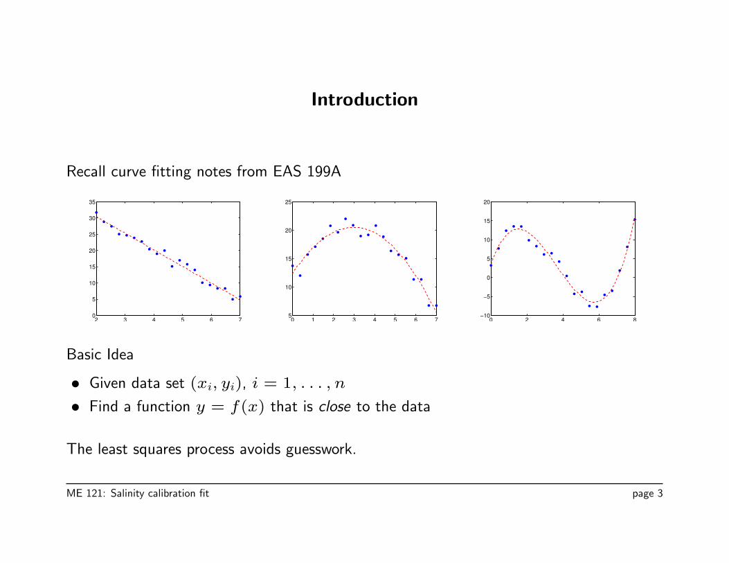
Recall curve fitting notes from EAS 199A
2 3 4 5 6 70
5
10
15
20
25
30
35
0 1 2 3 4 5 6 75
10
15
20
25
0 2 4 6 8−10
−5
0
5
10
15
20
Basic Idea
• Given data set (xi, yi), i = 1, . . . , n
• Find a function y = f(x) that is close to the data
The least squares process avoids guesswork.
ME 121: Salinity calibration fit page 3
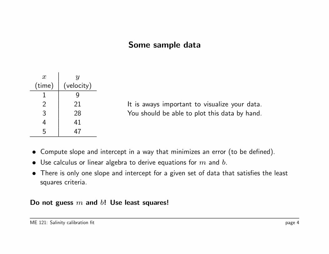
Some sample data
x y
(time) (velocity)
1 9
2 21
3 28
4 41
5 47
It is aways important to visualize your data.
You should be able to plot this data by hand.
• Compute slope and intercept in a way that minimizes an error (to be defined).
• Use calculus or linear algebra to derive equations for m and b.
• There is only one slope and intercept for a given set of data that satisfies the least
squares criteria.
Do not guess m and b! Use least squares!
ME 121: Salinity calibration fit page 4

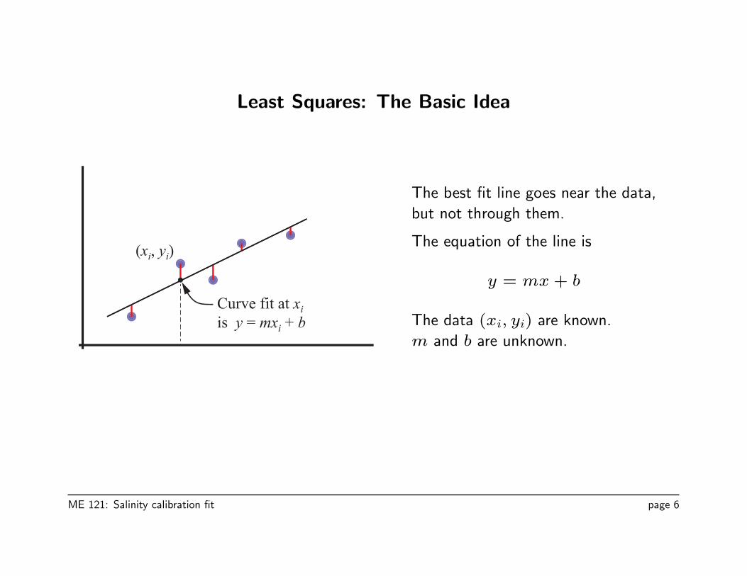
Least Squares: The Basic Idea
The best fit line goes near the data,
but not through them.
ME 121: Salinity calibration fit page 5
Least Squares: The Basic Idea
Curve fit at xiis y = mxi + b
(xi, yi)
The best fit line goes near the data,
but not through them.
The equation of the line is
y = mx+ b
The data (xi, yi) are known.
m and b are unknown.
ME 121: Salinity calibration fit page 6
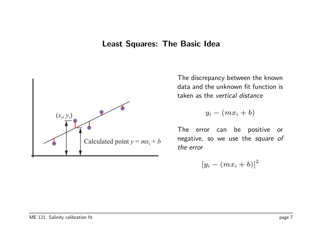
Least Squares: The Basic Idea
Calculated point y = mxi + b
(xi, yi)
The discrepancy between the known
data and the unknown fit function is
taken as the vertical distance
yi − (mxi + b)
The error can be positive or
negative, so we use the square of
the error
[yi − (mxi + b)]2
ME 121: Salinity calibration fit page 7
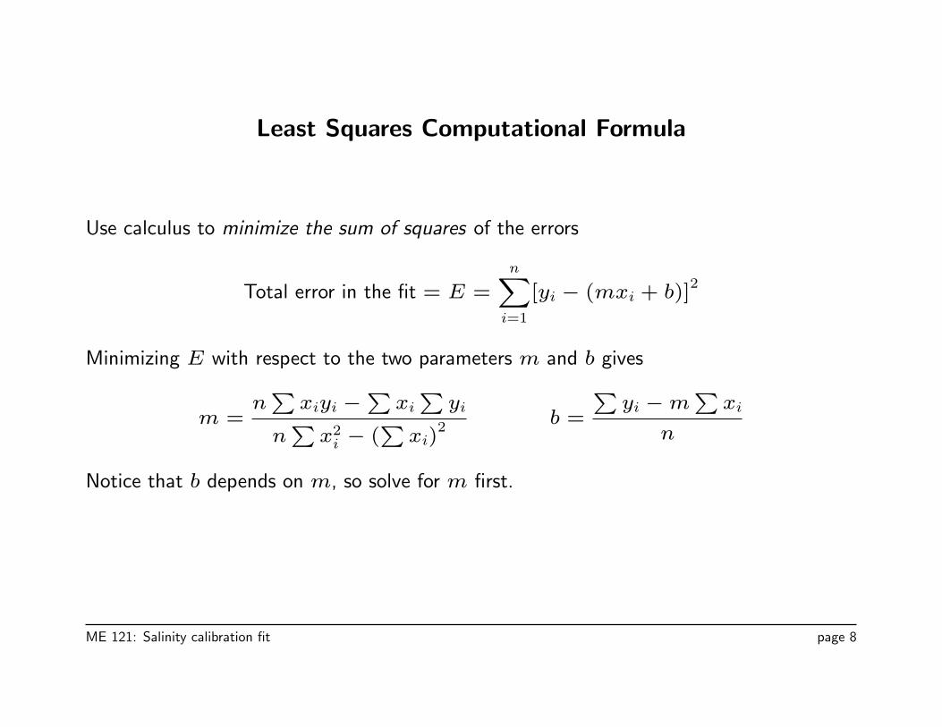
Least Squares Computational Formula
Use calculus to minimize the sum of squares of the errors
Total error in the fit = E =
n∑i=1
[yi − (mxi + b)]2
Minimizing E with respect to the two parameters m and b gives
m =n∑xiyi −
∑xi
∑yi
n∑x2i − (
∑xi)
2b =
∑yi −m
∑xi
n
Notice that b depends on m, so solve for m first.
ME 121: Salinity calibration fit page 8
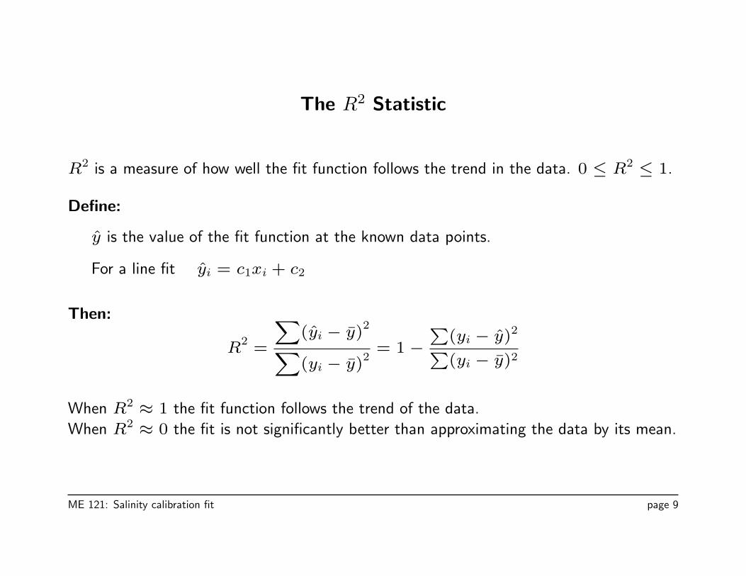
The R2 Statistic
R2 is a measure of how well the fit function follows the trend in the data. 0 ≤ R2 ≤ 1.
Define:
y is the value of the fit function at the known data points.
For a line fit yi = c1xi + c2
Then:
R2
=
∑(yi − y)
2∑(yi − y)
2= 1−
∑(yi − y)2∑(yi − y)2
When R2 ≈ 1 the fit function follows the trend of the data.
When R2 ≈ 0 the fit is not significantly better than approximating the data by its mean.
ME 121: Salinity calibration fit page 9
Least Squares Polynomial Curve Fit
The procedure for fitting a line to data can be extended to fitting a polynomial to data.
The basic ideas are the same, but the algebra is more involved. Here we just give the
highlights.
ME 121: Salinity calibration fit page 10
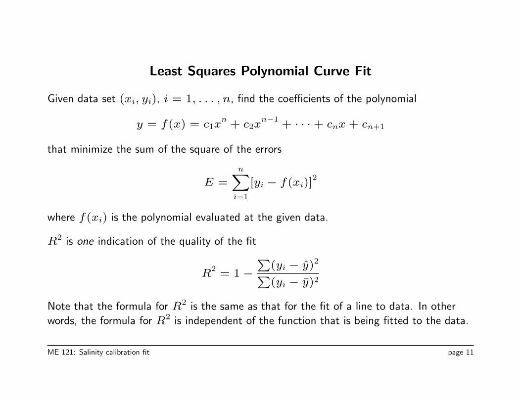
Least Squares Polynomial Curve Fit
Given data set (xi, yi), i = 1, . . . , n, find the coefficients of the polynomial
y = f(x) = c1xn
+ c2xn−1
+ · · ·+ cnx+ cn+1
that minimize the sum of the square of the errors
E =
n∑i=1
[yi − f(xi)]2
where f(xi) is the polynomial evaluated at the given data.
R2 is one indication of the quality of the fit
R2
= 1−∑
(yi − y)2∑(yi − y)2
Note that the formula for R2 is the same as that for the fit of a line to data. In other
words, the formula for R2 is independent of the function that is being fitted to the data.
ME 121: Salinity calibration fit page 11
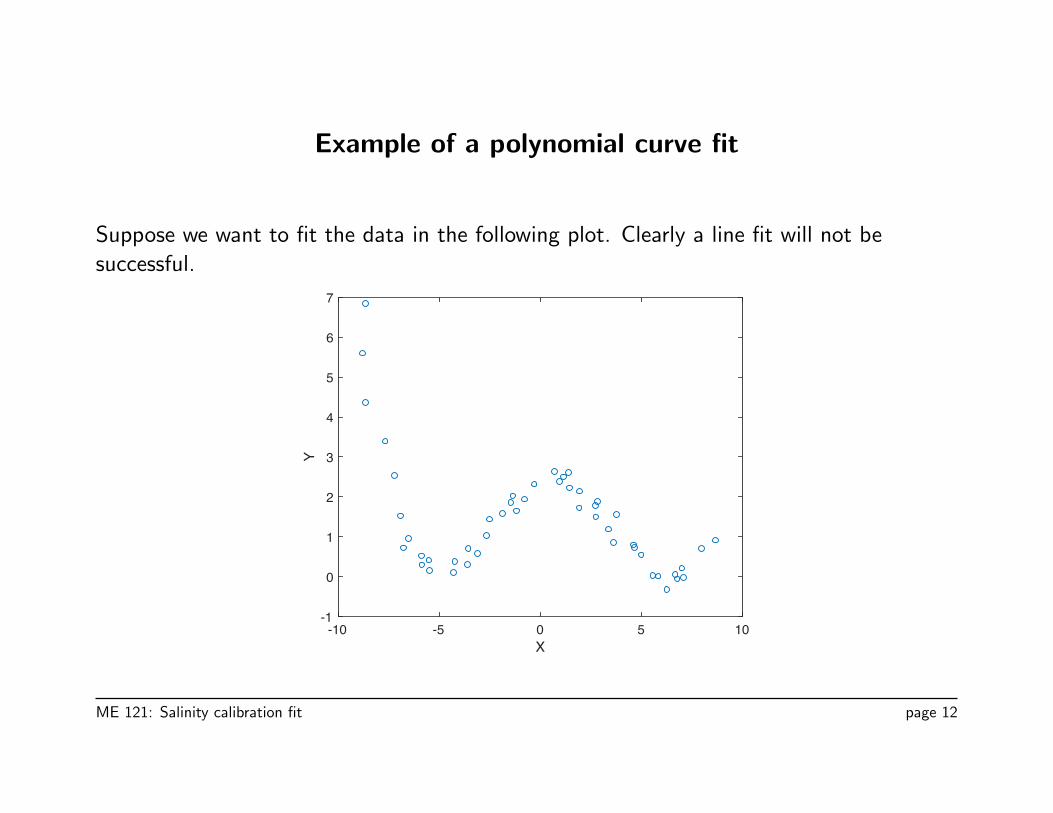
Example of a polynomial curve fit
Suppose we want to fit the data in the following plot. Clearly a line fit will not be
successful.
-10 -5 0 5 10X
-1
0
1
2
3
4
5
6
7Y
ME 121: Salinity calibration fit page 12
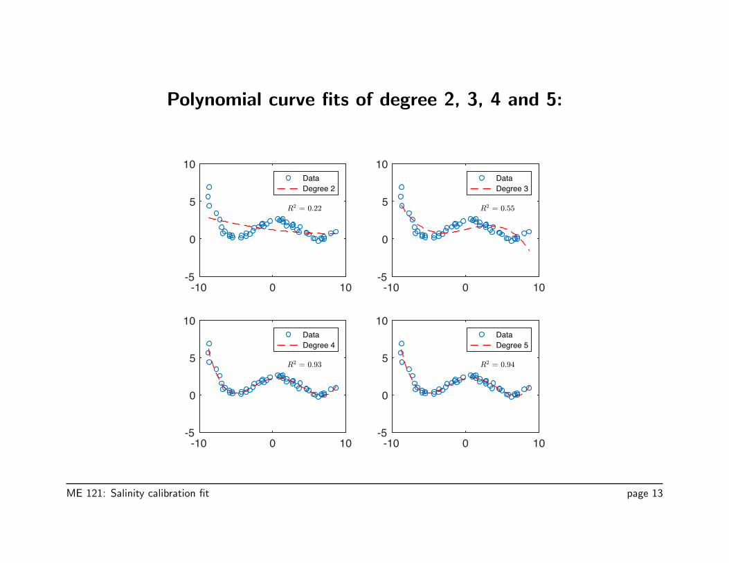
Polynomial curve fits of degree 2, 3, 4 and 5:
-10 0 10-5
0
5
10DataDegree 2
-10 0 10-5
0
5
10DataDegree 3
-10 0 10-5
0
5
10DataDegree 4
-10 0 10-5
0
5
10DataDegree 5
ME 121: Salinity calibration fit page 13
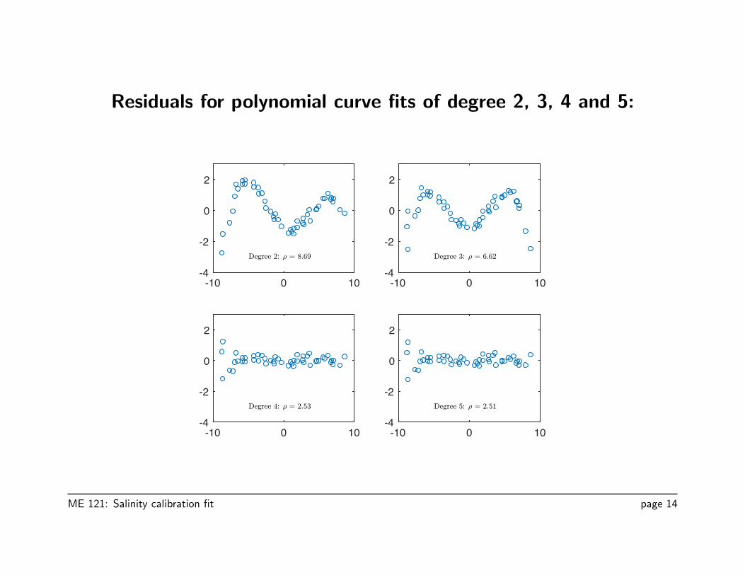
Residuals for polynomial curve fits of degree 2, 3, 4 and 5:
-10 0 10-4
-2
0
2
-10 0 10-4
-2
0
2
-10 0 10-4
-2
0
2
-10 0 10-4
-2
0
2
ME 121: Salinity calibration fit page 14
2. Introduction to least squares curve fitting with Matlab
ME 121: Salinity calibration fit page 15
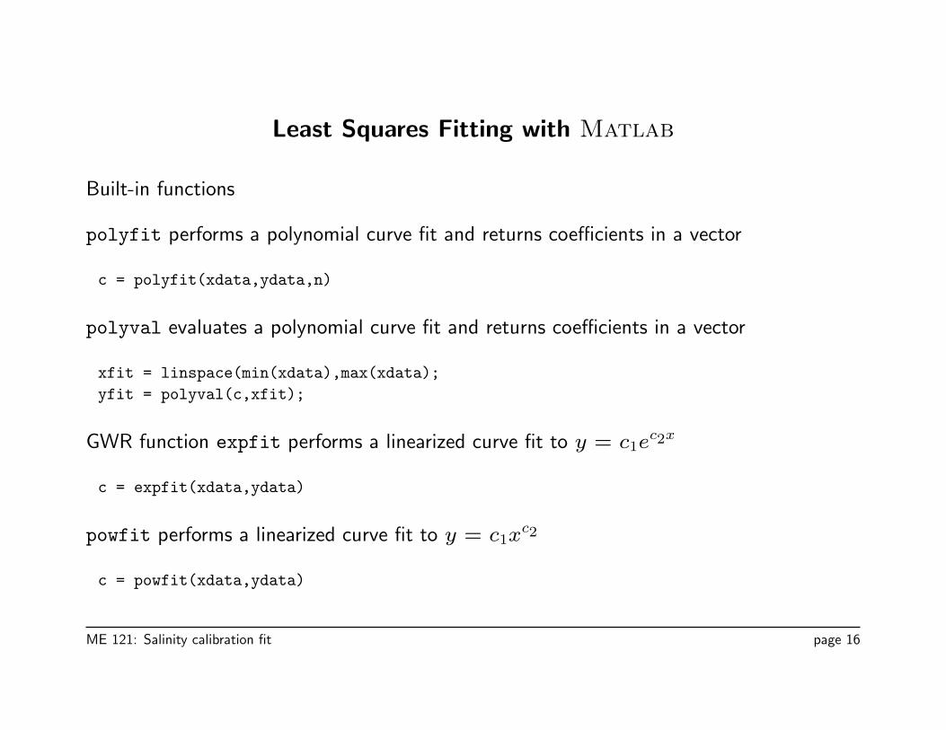
Least Squares Fitting with Matlab
Built-in functions
polyfit performs a polynomial curve fit and returns coefficients in a vector
c = polyfit(xdata,ydata,n)
polyval evaluates a polynomial curve fit and returns coefficients in a vector
xfit = linspace(min(xdata),max(xdata);
yfit = polyval(c,xfit);
GWR function expfit performs a linearized curve fit to y = c1ec2x
c = expfit(xdata,ydata)
powfit performs a linearized curve fit to y = c1xc2
c = powfit(xdata,ydata)
ME 121: Salinity calibration fit page 16
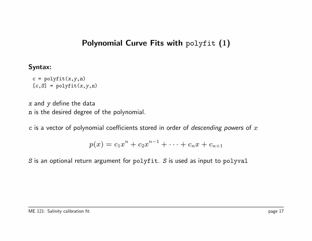
Polynomial Curve Fits with polyfit (1)
Syntax:
c = polyfit(x,y,n)
[c,S] = polyfit(x,y,n)
x and y define the data
n is the desired degree of the polynomial.
c is a vector of polynomial coefficients stored in order of descending powers of x
p(x) = c1xn
+ c2xn−1
+ · · ·+ cnx+ cn+1
S is an optional return argument for polyfit. S is used as input to polyval
ME 121: Salinity calibration fit page 17
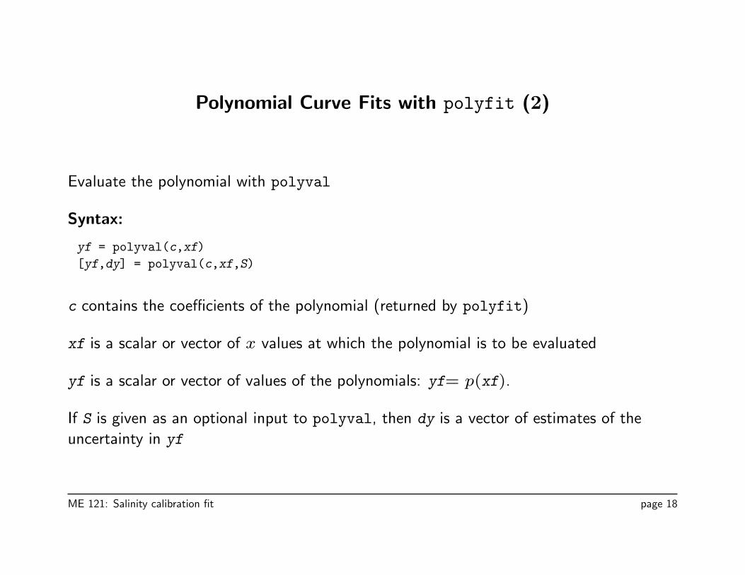
Polynomial Curve Fits with polyfit (2)
Evaluate the polynomial with polyval
Syntax:
yf = polyval(c,xf)
[yf,dy] = polyval(c,xf,S)
c contains the coefficients of the polynomial (returned by polyfit)
xf is a scalar or vector of x values at which the polynomial is to be evaluated
yf is a scalar or vector of values of the polynomials: yf= p(xf).
If S is given as an optional input to polyval, then dy is a vector of estimates of the
uncertainty in yf
ME 121: Salinity calibration fit page 18
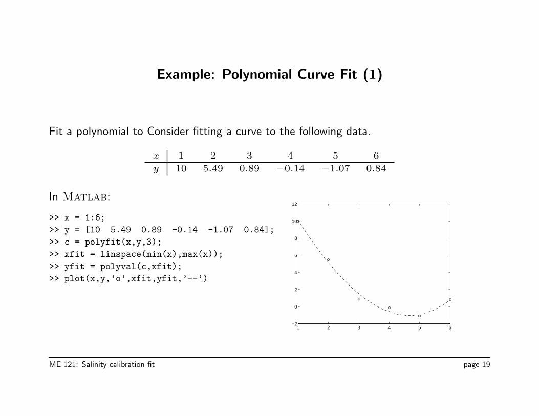
Example: Polynomial Curve Fit (1)
Fit a polynomial to Consider fitting a curve to the following data.
x 1 2 3 4 5 6
y 10 5.49 0.89 −0.14 −1.07 0.84
In Matlab:
>> x = 1:6;
>> y = [10 5.49 0.89 -0.14 -1.07 0.84];
>> c = polyfit(x,y,3);
>> xfit = linspace(min(x),max(x));
>> yfit = polyval(c,xfit);
>> plot(x,y,’o’,xfit,yfit,’--’)
1 2 3 4 5 6−2
0
2
4
6
8
10
12
ME 121: Salinity calibration fit page 19
Fitting Transformed Non-linear Functions (1)
• Some nonlinear fit functions y = F (x) can be transformed to an equation of the
form v = αu+ β
• perform a linear least squares fit on the transformed variables.
• Parameters of the nonlinear fit function are obtained by transforming back to the
original variables.
• The linear least squares fit to the transformed equations does not yield the same fit
coefficients as a direct solution to the nonlinear least squares problem involving the
original fit function.
Examples:
y = c1ec2x −→ ln y = αx+ β
y = c1xc2 −→ ln y = α ln x+ β
y = c1xec2x −→ ln(y/x) = αx+ β
ME 121: Salinity calibration fit page 20
Fitting Transformed Non-linear Functions (2)
Consider
y = c1ec2x (1)
Taking the logarithm of both sides yields
ln y = ln c1 + c2x
Introducing the variables
v = ln y b = ln c1 a = c2
transforms equation (1) to
v = ax+ b
ME 121: Salinity calibration fit page 21
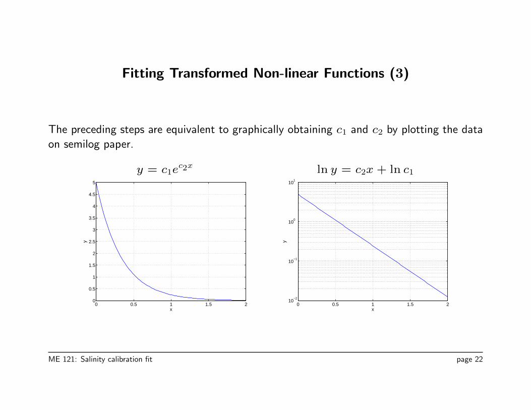
Fitting Transformed Non-linear Functions (3)
The preceding steps are equivalent to graphically obtaining c1 and c2 by plotting the data
on semilog paper.
y = c1ec2x ln y = c2x+ ln c1
0 0.5 1 1.5 20
0.5
1
1.5
2
2.5
3
3.5
4
4.5
5
x
y
0 0.5 1 1.5 210
−2
10−1
100
101
x
y
ME 121: Salinity calibration fit page 22
Fitting Transformed Non-linear Functions (4)
Consider y = c1xc2. Taking the logarithm of both sides yields
ln y = ln c1 + c2 ln x (2)
Introduce the transformed variables
v = ln y u = ln x b = ln c1 a = c2
and equation (2) can be written
v = au+ b
ME 121: Salinity calibration fit page 23
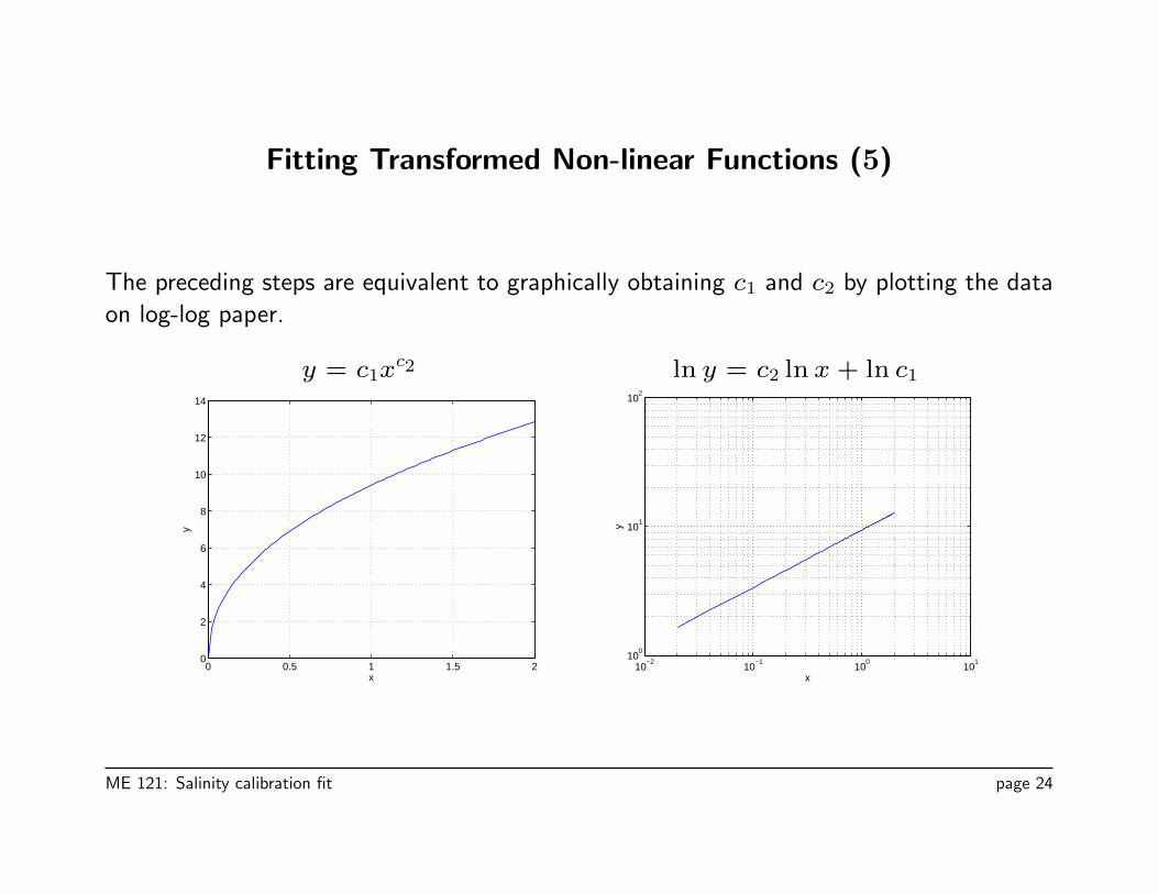
Fitting Transformed Non-linear Functions (5)
The preceding steps are equivalent to graphically obtaining c1 and c2 by plotting the data
on log-log paper.
y = c1xc2 ln y = c2 ln x+ ln c1
0 0.5 1 1.5 20
2
4
6
8
10
12
14
x
y
10−2
10−1
100
101
100
101
102
x
y
ME 121: Salinity calibration fit page 24
3. Application to calibration of the salinity sensor
ME 121: Salinity calibration fit page 25
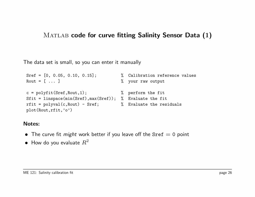
Matlab code for curve fitting Salinity Sensor Data (1)
The data set is small, so you can enter it manually
Sref = [0, 0.05, 0.10, 0.15]; % Calibration reference values
Rout = [ ... ] % your raw output
c = polyfit(Sref,Rout,1); % perform the fit
Sfit = linspace(min(Sref),max(Sref)); % Evaluate the fit
rfit = polyval(c,Rout) - Sref; % Evaluate the residuals
plot(Rout,rfit,’o’)
Notes:
• The curve fit might work better if you leave off the Sref = 0 point
• How do you evaluate R2
ME 121: Salinity calibration fit page 26
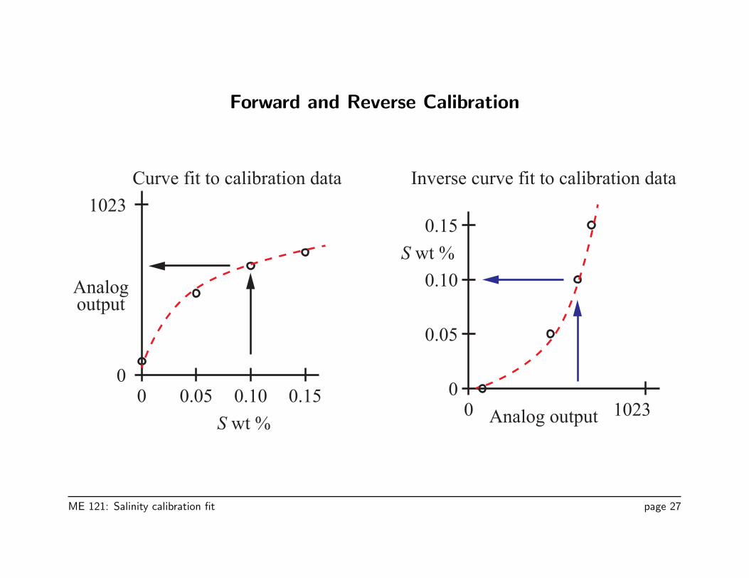
Forward and Reverse Calibration
Analogoutput
S wt %
S wt %
Curve fit to calibration data
Analog output0
0
0
1023
102300.05
0.05
0.10
0.10
0.15
0.15
Inverse curve fit to calibration data
ME 121: Salinity calibration fit page 27
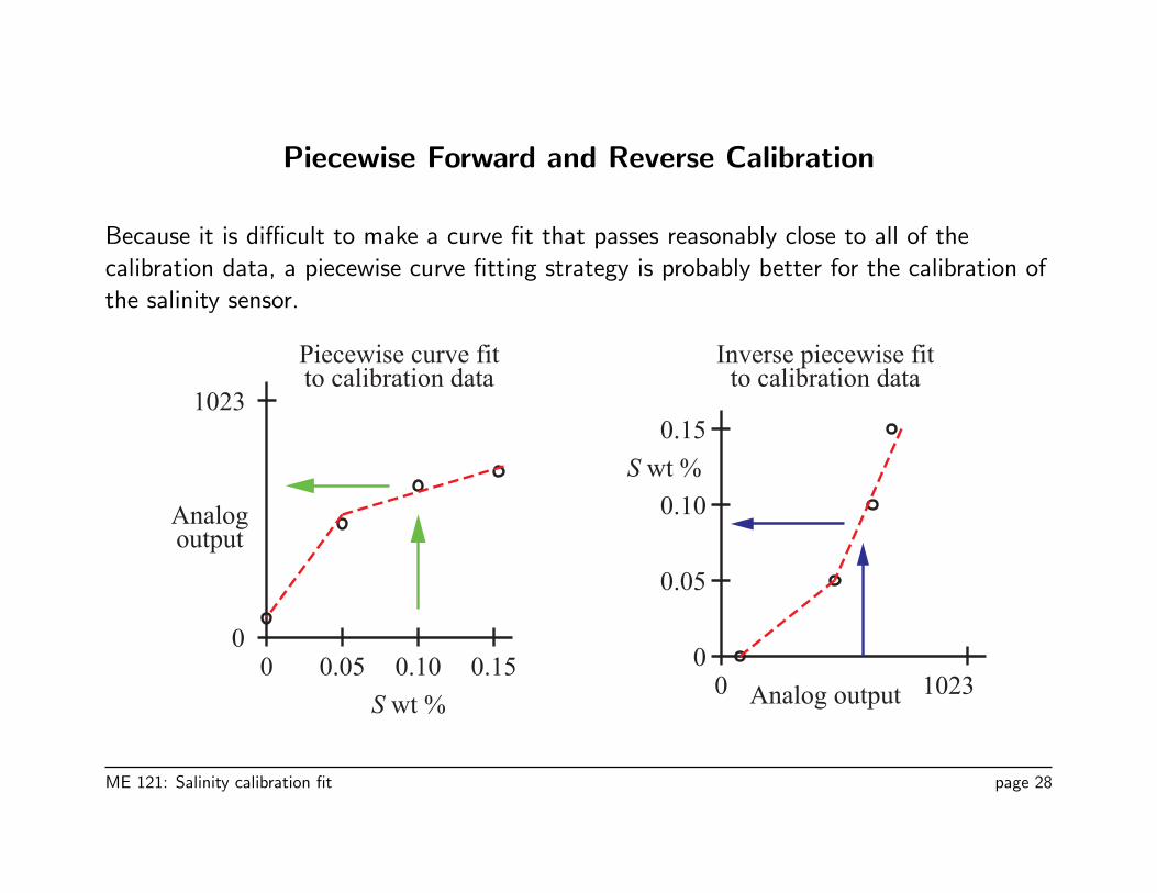
Piecewise Forward and Reverse Calibration
Because it is difficult to make a curve fit that passes reasonably close to all of the
calibration data, a piecewise curve fitting strategy is probably better for the calibration of
the salinity sensor.
Analogoutput
S wt %
S wt %
Piecewise curve fitto calibration data
Analog output0
0
0
1023
102300.05
0.05
0.10
0.10
0.15
0.15
Inverse piecewise fitto calibration data
ME 121: Salinity calibration fit page 28

![Fabrication of a Centrifugal Pump - start [ME 120]me120.mme.pdx.edu/lib/exe/fetch.php?media=lecture:pump... · 2015-03-11 · Tap into pump body outlet Tap 1/8 inch 27 NPT threads](https://img.pdfslide.net/doc/110x75/5e81391a1ed74d02ec637f7e/fabrication-of-a-centrifugal-pump-start-me-120me120mmepdxedulibexefetchphpmedialecturepump.jpg)
![Arduino Programming Part 1 - start [ME 120]me120.mme.pdx.edu/lib/exe/fetch.php?media=lecture:arduino_programming_2.pdfME 120: Arduino Programming Assigning values The equals sign is](https://img.pdfslide.net/doc/110x75/5e286e1603c819281b417c20/arduino-programming-part-1-start-me-120me120mmepdxedulibexefetchphpmedialecturearduinoprogramming2pdf.jpg)