Contract No.: 0600-01-60121/5500-05-31358 MPR Reference No.: 6193-501

Sample Loss and Survey Bias in Estimates of Social Security Beneficiaries: A Tale of Two Surveys Final Report February 2008 John L. Czajka James Mabli Scott Cody

Submitted to:

Social Security Administration Office of Research, Evaluation and Statistics ITC Building, 9th Floor 500 E Street, SW Washington, DC 20254

Attention: Jim Sears

Technical Representative

Submitted by:

Mathematica Policy Research, Inc. 600 Maryland Ave., SW, Suite 550 Washington, DC 20024-2512 Telephone: (202) 484-9220 Facsimile: (202) 863-1763

Project Director:

John L. Czajka

iii

ACKNOWLEDGMENTS

The authors would like to acknowledge the contributions of several individuals to the preparation of this report. We are especially grateful to Julie Sykes, who programmed most of the estimates presented herein and to Miriam Loewenberg, who ran Julie’s programs on a Social Security Administration (SSA) computer. Without their skilled programming, long hours, and attention to detail this report would not have been possible. We also want to thank Daisy Ewell and Sandra Nelson for preparing a number of additional tabulations outside of the SSA environment. We are grateful, as well, to Dan Kasprzyk for reviewing a preliminary draft of this report; to Karen Cunnyngham for tremendous assistance with the SSA administrative data and in the identification of Social Security beneficiary status in the Current Population Survey and Survey of Income and Program Participation; and to Joel Smith for reviewing the documentation and programs for the calibration methodology and demonstrating that someone outside the project could replicate the results.

This report benefited greatly from the assistance of an expert panel combining many decades

of experience in survey methodology. We gratefully acknowledge the contributions of our panelists: Christopher Bollinger, Michael Davern, Arthur Kennickell, Nathaniel Schenker and Fritz Scheuren.

Finally, we want to thank our project officer, Jim Sears, and his colleagues Howard Iams

and Paul Davies at SSA, the sponsoring agency, for assisting us in working with the SSA data, providing helpful guidance, answering many questions, and encouraging us to pursue the key research questions to a full resolution.

v

CONTENTS

Chapter Page ACKNOWLEDGMENTS .................................................................................... iii EXECUTIVE SUMMARY ...................................................................................ix I. INTRODUCTION ..................................................................................................1 II. SAMPLE LOSS IN THE SIPP AND CPS .............................................................9 A. NONRESPONSE ............................................................................................9 1. Nonresponse in the SIPP ..........................................................................9 2. Nonresponse in the CPS .........................................................................18 B. NONMATCHING .........................................................................................19 1. How the Census Bureau Matches Survey and Administrative Records .20 2. Match Rates in the CPS ..........................................................................21 3. Match Rates in the SIPP .........................................................................23 4. Combined Sample Loss from SIPP Attrition and Nonmatching.............25 5. What Can We Expect in the Future? ......................................................26 C. CONCLUSION .............................................................................................27 Tables ............................................................................................................30 III. MATCH BIAS IN THE SIPP AND CPS .............................................................41 A. EVALUATING MATCH BIAS ...................................................................41 B. MATCH BIAS IN THE SIPP .......................................................................45

1. Comparison of Matched Respondents and All Respondents in the 2001 Panel ........................................................46

2. Eligibility for SSI ...................................................................................50 3. Pension Coverage of Divorced Women .................................................55

C. MATCH BIAS IN THE CPS ........................................................................57 D. CONCLUSION .............................................................................................60 Tables ............................................................................................................62 IV. ATTRITION BIAS IN THE SIPP ........................................................................85 A. EVALUATING ATTRITION BIAS .............................................................85 B. ASSESSMENT BASED ON SIPP CHARACTERISTICS ..........................90

vi

Chapter Page

C. ASSESSMENT BASED ON MATCHED ADMINISTRATIVE RECORDS .................................................................93

1. Bias in Full Panel Estimates of Earnings ...............................................94 2. Bias in Full Panel Estimates of Social Security Beneficiaries ...............98 3. Bias in Full Panel Estimates of SSI Recipients ....................................101 4. Attrition Bias in the 1996 Panel ...........................................................103 D. CONCLUSION ...........................................................................................109 Tables ..........................................................................................................111 Figures .........................................................................................................125 V. CROSS-SECTIONAL REPRESENTATIVENESS OVER TIME ....................133

A. CHARACTERISTICS OF DISABLED WORKERS AND SSI RECIPIENTS ..............................................................................134

B. MONTHLY POVERTY ..............................................................................137 1. Possible Sources of Discontinuity between Panels ..............................138 2. Discontinuities by Age .........................................................................142 C. SOURCES OF BIAS IN SIPP CROSS-SECTIONAL ESTIMATES .........143 1. Attrition ................................................................................................144 2. Additions to the Population ..................................................................148 D. CONCLUSION ...........................................................................................155 Tables ..........................................................................................................157 Figures .........................................................................................................167

VI. MEASUREMENT OF ECONOMIC WELL-BEING IN THE SIPP AND CPS ............................................................................................173

A. SOURCES OF INCOME ............................................................................174 1. Reliance upon Social Security Benefits ...............................................174 2. Sources of Income among All Persons by Age ....................................178 B. AGGREGATE INCOME ............................................................................183 1. Comparative Estimates of Aggregate Income ......................................184 2. Income by Quintile ...............................................................................186 3. Proportion of Income That Is Imputed .................................................190

vii

Chapter Page C. POVERTY RATES .....................................................................................197 1. Poverty Trends in the SIPP and CPS ...................................................198 2. Poverty Trends by Age .........................................................................200 D. CONCLUSION ...........................................................................................203 Tables ..........................................................................................................207 Figures .........................................................................................................227 VII. CONCLUSION AND RECOMMENDATIONS ...............................................233 REFERENCES ...................................................................................................239 APPENDIX A: CALIBRATION OF SAMPLES APPENDIX B: USE OF REPLICATE WEIGHTS TO CALCULATE STANDARD ERRORS FOR THE SIPP APPENDIX C: COMPARISON OF MATCHED AND ENTIRE WAVE 1/WAVE 2 SAMPLES: 2001 SIPP PANEL APPENDIX D: COMPARISON OF DIFFERENCES BETWEEN MATCHED AND ENTIRE WAVE 1/WAVE 2 SAMPLES: 1996 AND 2001 SIPP PANELS APPENDIX E: COMPARISON OF DIFFERENCES BETWEEN MATCHED AND ENTIRE FULL PANEL SAMPLES: 1996 AND 2001 SIPP PANELS APPENDIX F: COMPARISON OF FULL PANEL AND CROSS- SECTION SAMPLES: 2001 SIPP PANEL APPENDIX G: COMPARISON OF FULL PANEL AND CROSS- SECTION SAMPLES: 1996 SIPP PANEL APPENDIX H: EVALUATION OF ATTRITION BIAS IN THE 1996 SIPP PANEL: TABLES AND FIGURES

ix

EXECUTIVE SUMMARY

The Office of Research, Evaluation, and Statistics (ORES) within the Social Security Administration (SSA) relies on data from the Census Bureau’s Survey of Income and Program Participation (SIPP) and the Current Population Survey (CPS) as a source of information on current and potential beneficiaries served by the programs that SSA administers. In addition to using these surveys directly, SSA links administrative records to the records of survey respondents who provide Social Security numbers (SSNs). These matched data expand the content of the SIPP and CPS files to fields available only through SSA and Internal Revenue Service (IRS) records—such as lifetime earnings histories and aspects of SSA program participation not collected in the surveys. The matched data also allow SSA to conduct validation studies of survey items that are duplicated in the administrative records or to substitute the generally more accurate administrative items for their survey counterparts, thereby creating composite records.

The continuing usefulness of these surveys for this wide range of applications is being

undercut by growing sample loss. One source of sample loss is survey nonresponse, which for the SIPP includes both initial nonresponse and attrition. Both have increased since the early 1990s. Another source of sample loss affecting SSA’s linked data is the reluctance of respondents to provide their SSNs, which prevents the Census Bureau from attempting a match between the survey records and the SSA and IRS administrative records. The growing reluctance of respondents to provide their SSNs is reflected in a declining match rate in the CPS. In the SIPP, match rates plunged between the 1996 and 2001 panels when the request for SSNs was moved from the initial or “first wave” interview, which is conducted in person, to the second wave interview, which is frequently conducted by telephone. Growth in both forms of sample loss raises questions about the continued representativeness of linked data from the two surveys—or even unmatched survey data from a three or four-year SIPP panel.

This report examines sample loss in the SIPP and CPS with an eye to telling SSA what to do

about it. Successive chapters document the growth in sample loss due to nonresponse and nonmatching; provide estimates of match bias and attrition bias; examine discontinuities between consecutive SIPP panels in estimates of beneficiary characteristics as well as poverty rates for the broader population; and examine the comparative strengths of the SIPP and CPS in describing the economic well-being of the population in general and elderly and lower-income persons in particular. A concluding chapter summarizes our major findings and presents a number of recommendations that follow from these findings.

Sample Loss in the SIPP and CPS

When measured in terms of the proportion of wave 1 respondents who were missing any months of data and, therefore, could not be assigned full panel weights, attrition got no worse between the 1996 and 2001 panels. Among older social security beneficiaries and older persons generally, attrition of this type was actually lower in the 2001 panel than the 1996 panel. Furthermore, because of an operational change to retain sample members who missed consecutive interviews, the proportion of the wave 1 sample failing to complete the wave 9 interview declined markedly between the 1996 and 2001 panels, to the point where the 2001

x

panel resembled the 1993 panel more closely than it resembled the 1996 panel with respect to this alternative measure of attrition. These developments imply that the upturn in attrition between the 1993 and 1996 panels did not continue through the 2001 panel. If concerns about increased attrition were a major factor in SSA staff’s reluctance to use the 2001 panel, these concerns would appear to be misplaced.

Unit nonresponse to the CPS ASEC supplement has grown very modestly since the mid-

1990s, but it is important to divide the unit nonresponse into two components. In ASEC months, CPS households are first administered the monthly labor force questionnaire followed by the ASEC supplement. About one in nine households that complete the brief labor force questionnaire do not complete the supplement. Historically, nonresponse to the monthly labor force survey has been very low. Noninterview rates deviated little from 4 to 5 percent of eligible households between 1960 and 1994 but then began a gradual rise coinciding with the introduction of a redesigned survey instrument using computer-assisted interviewing. By March 1997 the noninterview rate had reached 7 percent, but it rose by just another percentage point over the next seven years. Over this same period, nonresponse to the March supplement among respondents to the labor force survey ranged between 8 and 9 percent, with no distinct trend, yielding a combined sample loss that varied between 14 and 16 percent of the eligible households. Defined in this way, overall nonresponse to the March or ASEC supplement is 2 to 3 percentage points higher than nonresponse to the first wave of the 2001 SIPP panel.

While attrition may not have grown between the 1996 and 2001 panels, the rate at which

respondents could be matched to administrative records dropped sharply. Excluding the 15 percent of respondents who were dropped from the sample after the first wave, only 60 percent of the initial respondents to the 2001 panel could be matched to administrative records compared to 83 percent of the respondents to the 1996 panel. When combined with the sample loss due to attrition, this meant that only 50 percent of the 2001 panel had both matched data and survey data through wave 9, and only 42 percent had both matched data and full panel data. In the 1996 panel these figures were 62 percent and 55 percent, respectively.

Between March 1996 and March 2001, match rates in the CPS declined from 84 percent to

74 percent over the sample as a whole, but they remained close to 90 percent for children under 15, who were matched using a methodology that was implemented for all CPS and SIPP respondents in 2006. As a result, we anticipate match rates approaching 90 percent for CPS ASEC supplements in 2006 and later and for the next SIPP panel. While this is a positive development, the possibility that the new record linkage methods might introduce new forms of match bias must be acknowledged and examined when data linked with the new methodology become available.

Match Bias in the SIPP and CPS

While the proportion of SIPP respondents who could be matched to SSA administrative records dropped precipitously between the 1996 and 2001 panels, this appears to have occurred without increasing the bias of the matched sample. When we calibrated the matched and total sample members who responded to both waves 1 and 2 of the 2001 panel to the same wave 1 demographic controls that the Census Bureau used to calibrate the full wave 1 sample, we found little evidence of bias in estimates of a wide range of characteristics, much less an increase relative to the 1996 panel. Analyses of three illustrative applications of matched data defined by

xi

SSA provided stronger evidence of bias in the matched subsample. Simulations of elderly SSI eligibility based on income alone as well as income combined with assets showed somewhat fewer persons eligible for SSI in the matched sample than the full sample. Yet even here we found no evidence that this possible bias increased between the 1996 and 2001 panels. Furthermore, it is possible that the differences we observe between the matched subsample and full sample can be attributed to full sample members who lack SSNS and, therefore, are not included in the population that the matched sample represents. If so, the differences do not reflect bias in the matched subsample at all but, rather, our inability to identify and restrict our comparisons to the “matchable universe” within the full sample.

Our more limited evaluation of match bias in the CPS focused on retired workers and

obtained results for that subpopulation that were very similar to what we found with the SIPP. For personal, family and household demographic characteristics the matched subsample mirrored the full sample. Small differences were observed for economic characteristics, with matched cases having slightly more income and being marginally less reliant on their Social Security benefits. These findings held when we restricted our analysis to those respondents who completed the annual supplement (as opposed to those whose data from the supplement were entirely imputed). As with the SIPP, the small bias that we detected would appear to be inconsequential for SSA’s potential uses of CPS data.

Attrition Bias in the SIPP

Comparative analysis of SIPP full panel and cross-sectional sample estimates of a wide

variety of characteristics measured in wave 1 of the 1996 and 2001 SIPP panels for the total population and four subpopulations of Social Security and SSI beneficiaries provides evidence that the Census Bureau’s full panel weights are highly effective in eliminating the effects of differential attrition on the full panel estimates of cross-sectional characteristics. Further analysis using subsamples of the full panel and cross-sectional samples matched to IRS earnings records and Social Security benefit records provides further evidence that the full panel sample with the Census Bureau’s panel weights can support largely unbiased estimates for characteristics and subpopulations of interest to SSA analysts.

Because it applies to the entire population, rather than just the elderly subpopulation with its

lower attrition rates, and because it was not limited to a single point in time, our analysis of IRS annual earnings data records matched to SIPP records is particularly compelling. For the 2001 SIPP panel we found no important differences between the full panel and cross-sectional sample estimates of the proportion of persons with positive earnings, by age, in any of the years 1999 through 2003. Differences in the distribution of earnings among those with positive earnings were generally small and rarely statistically significant. Where there appeared to be a pattern in these differences, among persons 55 to 64, it ran counter to what is known about differential attrition by income—that is, the panel sample had somewhat lower rather than higher earnings than the cross-sectional sample. Estimates of gross changes in earnings also differed little between the full panel and wave 1/wave 2 cross-sectional samples.

We replicated this analysis on the 1996 panel so that we could include cross-sectional

sample members who attrited between the first and second waves. As with the 2001 panel we found no important differences in the proportion of persons with positive earnings in any of the five years we examined (1994 through 1998). There was stronger evidence of differential

xii

earnings between the full panel and cross-sectional samples, particularly at ages 55 and up, but the percentile distributions of earnings lined up quite closely through the 80th percentile. At higher income levels the full panel underestimated the number of higher earners (yielded lower percentile values) relative to the cross-sectional sample, but these differences are beyond the level where SSA policy analysts would focus most of their attention.

Estimates of the number and selected characteristics of Social Security and SSI beneficiaries

show only small differences between the full panel and cross-sectional samples for both panels. This is particularly striking for estimates of transitions into and out of Social Security beneficiary categories, estimates of payment amounts for retired and disabled workers, and estimates of the proportion of Social Security and SSI beneficiaries’ personal income that is provided by their respective programs.

Cross-sectional Representativeness over Time In order to maintain full cross-sectional representativeness, a panel survey requires two elements in its design. First, the survey must have a viable mechanism for adding new sample members to represent additions to the population from which the panel was originally selected. Second, the survey must have an effective means of compensating for nonrandom attrition. If a panel survey lacks either of these elements, it will become increasingly less representative of the full population over time. New entrants are represented in the SIPP only to the extent that they move in with persons who were included in the SIPP universe at the start of a panel. In addition, the cross-sectional weights are calibrated to population totals that include new entrants. Our research indicates that the SIPP longitudinal weights incorporate a highly effective adjustment for nonrandom attrition, but our findings do not address the adequacy of the cross-sectional weights, which cannot be evaluated by the same methods. We note, however, that the attrition adjustment that is incorporated into the cross-sectional weights is very similar in design to the attrition adjustment that works so well in the longitudinal weights. Estimates of non-income-related characteristics of disabled workers and SSI recipients show high levels of consistency across the 1996 and 2001 SIPP panels, but this is not true of poverty estimates, which show marked discontinuities that vary by age. These discontinuities have been attributed to the cumulative effects of attrition within a panel. While only one of the last three SIPP panels shows declining poverty estimates over time, each panel has started with a markedly higher poverty rate than the previous one. Upon exploring this phenomenon further, however, we find that we can attribute a substantial portion of the discontinuity to a tendency for SIPP panels since 1996 to obtain high estimates of poverty in the first wave, which then decline sharply in the second wave. Much of the remaining discontinuity could be due to a phenomenon which has been largely overlooked in assessments of the representativeness of panel surveys over time—namely, the bias arising from the general lack of representation of new entrants to the population. Our evidence of the potential bias resulting from this source is indirect at best, but we establish the more general point that the new entrants who are excluded from a panel over time constitute a distinctive group that is large enough and potentially unique enough to induce marked shifts in poverty when they are suddenly represented in full by a new panel.

xiii

Measurement of Economic Well-being in the SIPP and CPS A comparison of SIPP and CPS estimates of the proportion of their personal and family income that retired workers obtain from Social Security raises serious concerns about using the CPS to examine issues related to reliance on Social Security income and, more generally, the sources of financial support among retired workers. The SIPP’s greater effectiveness in capturing income from multiple sources among Social Security retired workers demonstrates an important way in which the SIPP appears to provide a better vehicle for policy analysis. Across all age groups—but particularly children and the elderly—the SIPP has continued to identify more sources of family income than the CPS. Among the elderly, the frequency of multiple reported sources grew over time in the SIPP but not the CPS. At younger ages, however, the frequency of multiple reported sources declined over time in both surveys, although somewhat more so in the CPS than the SIPP. With respect to income amounts, however, the SIPP has lost ground to the CPS since the initial SIPP panel. From 1993 on, the most significant losses have occurred in the bottom income quintile, where the SIPP has historically performed best relative to the CPS. In 1993 the SIPP captured 20 percent more aggregate income from this income than did the CPS. By 2002, however, the SIPP’s advantage had fallen to just 6 percent. These losses were distributed across most income sources. Only for SSI, welfare and pensions did the SIPP maintain or improve its advantage. The transition to computer-based data collection appears to have been more beneficial to the CPS than the SIPP. The CPS estimate of total income improved by nearly 4 percentage points relative to a benchmark in the year that computer-assisted interviewing was introduced (reference year 1993), and it remained slightly above that level over the next three years. The SIPP estimate of total income improved by a percentage point when computer-assisted interviewing was introduced in 1996, but a Census Bureau evaluation ends in that year, so we cannot tell if the SIPP maintained that level of coverage relative to the benchmark. The proportion of income that is imputed rose substantially in both surveys between 1993 and 2003. Three sources of income in the SIPP experienced particularly large increases. While there was evidence of a deterioration in the quality of imputations for one or two of these sources in the SIPP, differences in imputation outcomes between the two surveys do not appear to have played a role in the decline in the SIPP’s capture of income among families in the bottom quintile of the income distribution. The SIPP’s reduced capture of income among lower-income families, relative to the CPS, appears to have had an impact on comparative poverty estimates between the two surveys. Over the whole population, the SIPP’s annual estimates of the proportion of persons in poverty, which once ran 2 to 3 percentage points below the corresponding CPS poverty rates, converged on the CPS rates between the 1992 and 2001 panels. Differences between the two surveys vary by age group, however, and nowhere are the differences more troubling than among the elderly, where trends not only across the two surveys but within each survey’s estimates over time. Finally, a comparison of poverty trends in the two surveys raises a number of concerns about the use of either survey for the measurement of trends in economic well-being. These

xiv

concerns are strongest for estimates of the elderly, which makes these findings particularly important for staff in ORES who rely on the SIPP—and, to a lesser extent, the CPS—for a wide range of applications. Recommendations Finding no evidence that attrition bias or match bias in the linking of administrative records to survey data has increased in the SIPP since the 1996 panel, we recommend that prospective users of SIPP data at SSA not hesitate to use the 2001 SIPP panel any more than they would hesitate to use the 1996 panel. Neither attrition bias nor match bias provides any more reason to avoid the 2001 panel than the earlier panel. While we did not find it necessary to develop complex adjustment methodologies to reduce attrition bias and match bias to acceptable levels, we do recommend that SSA analysts make use of the calibration procedures that we applied to reweight matched subsamples of SIPP and CPS records to agree with full sample population totals by selected demographic characteristics. We recommend that SSA analysts apply the calibration procedures to their matched samples before applying any additional controls to meet program administrative totals. Despite the reduced match rate in the 2001 SIPP panel, SSA analysts should not combine matched and unmatched records for analyses of program beneficiaries. The matched records, when properly calibrated, will have sufficiently low bias—certainly no worse than the 1996 panel. With the Census Bureau undertaking a complete re-engineering of the SIPP, this report is especially timely. It is critically important that the Census Bureau and SIPP users who might be moved to influence the design of the new SIPP understand the current survey’s strengths and limitations, or the re-engineering effort will not achieve all that it could achieve. Indeed, if the re-engineering focuses on the wrong features, the new survey could prove to be decidedly inferior to the current survey. Two areas of concern stand out. The first is the wave 1 effect that we documented in Chapter V. Only the Census Bureau is in a position to explore this further, as the source of the problem may lie in field operations or the survey processing that occurs after the data have come in from the field. If the Census Bureau moves to an annual interview in the re-engineered SIPP, it is critical that the initial interview not reflect the same problem that we are seeing with the wave 1 SIPP interview. The second area of concern stems from the divergent trends in elderly poverty portrayed in the last chapter. The findings presented therein challenge users to reassess their reliance on either the CPS or the SIPP to measure the material well-being of the elderly either cross-sectionally or over time. We recommend that ORES encourage the Census Bureau to undertake an assessment of how these two surveys can present such inconsistent pictures of changes in elderly poverty over time. Only with a better understanding of the causes of these inconsistencies can users of either survey feel confidence in the information that they are able to extract from SIPP or CPS data.

1

I. INTRODUCTION

The Office of Research, Evaluation, and Statistics (ORES) within the Social Security

Administration (SSA) relies on data from the Census Bureau’s Survey of Income and Program

Participation (SIPP) and the Current Population Survey (CPS) as a source of information on

current and potential beneficiaries served by the programs that SSA administers. For instance,

SSA uses the SIPP to obtain detailed, monthly information on employment and income plus

periodic data on assets and selected types of expenditures. The SIPP also provides information

on monthly participation in programs in addition to the SSA programs, Old Age, Survivors and

Disability Income (OASDI) and Supplemental Security Income (SSI). From the CPS, SSA

obtains point-in-time information on labor force participation as well as data on annual income

and program participation for the previous calendar year.

In addition to using these surveys directly, SSA links administrative records to the records of

survey respondents who provide Social Security numbers (SSNs). These matched data expand

the content of the SIPP and CPS files to fields available only through SSA and Internal Revenue

Service (IRS) records—such as lifetime earnings histories and aspects of SSA program

participation not collected in the surveys. The matched data also allow SSA to conduct

validation studies of survey items that are duplicated in the administrative records or to substitute

the generally more accurate administrative items for their survey counterparts, thereby creating

composite records. SSA publishes tabulations based on these matched data, using a mix of items

from the survey and administrative records.

An additional application of SIPP data is the construction of microsimulation models that

build on the survey files by merging them with data from other sources through “statistical

matching” and other mechanisms designed to combine information from the records of similar

2

people rather than the same people. These models include the Modeling Income in the Near

Term (MINT) model, used to project retirement income and the well-being of retirees, and an

SSI model, used to simulate income and asset eligibility for the program. SSA uses these models

for a variety of analyses extending beyond descriptive tabulations of current or past beneficiary

characteristics.

The continuing usefulness of these surveys for this wide range of applications is being

undercut by growing sample loss. One source of sample loss is survey nonresponse, which for

the SIPP includes both initial nonresponse and attrition.1 Since the early 1990s, initial response

rates in the SIPP have fallen and attrition has risen—the precise magnitudes of these changes

being among the topics addressed in this report. CPS response rates have dropped as well,

reflecting a secular decline in survey response rates rather than something peculiar to these two

surveys. Another source of sample loss affecting SSA’s linked data is the reluctance of

respondents to provide their SSNs, which prevents the Census Bureau from attempting a match

between the survey records and the SSA and IRS administrative records. The growing

reluctance of respondents to provide their SSNs is reflected in a declining match rate in the CPS.

In the SIPP, match rates plunged between the 1996 and 2001 panels when the request for SSNs

was moved from the initial or “first wave” interview, which is conducted in person, to the second

wave interview, which is frequently conducted by telephone. While respondents’ growing

reluctance to provide SSNs was undoubtedly a factor, clearly other forces were at work.

Growth in both forms of sample loss raises questions about the continued representativeness

of linked data from the two surveys—or even unmatched survey data from a three or four-year

SIPP panel. These concerns are not merely theoretical. In 2001, SSA initiated publication of an

1 Attrition occurs in the CPS as well as the SIPP because the monthly labor force survey has a longitudinal

design. Because SSA does not make use of the longitudinal features of the CPS sample, however, attrition is not differentiated from initial nonresponse as a source of sample loss.

3

annual series of descriptive tabulations on disabled workers and SSI recipients, based on SIPP

data matched to administrative records. Five years later, SSA ceased publication of the tables,

citing growing attrition in the SIPP and increasingly lower match rates to administrative records.

ORES staff have also shown a general reluctance to use the 2001 SIPP panel for their analyses of

SSA beneficiaries.

In using data from the SIPP and CPS, SSA relies on the Census Bureau’s nonresponse

adjustments to compensate for initial nonresponse and attrition. While these adjustments may be

adequate for general population analysis, SSA is appropriately concerned about their

effectiveness for the subpopulations in which the agency is interested—that is, its current and

prospective beneficiaries and the comparison groups used in analyses. Furthermore, the Census

Bureau’s own research on attrition has demonstrated the presence of bias in the data with respect

to characteristics of interest to SSA—including employment, earnings, and the incidence of low

income (see Weinberg 2003 for a summary).

For the matched data, there are no Census Bureau adjustments that can be used to

compensate for possible bias. In using the matched data, therefore, SSA must apply its own

adjustments, or use none. SSA has routinely applied ratio adjustments to the weights of its

matched records in order to hit program enrollment totals, from which rough estimates of

institutionalized beneficiaries have been removed. Typically the control totals are broken down

by broad age groups but little else. When match rates are high the ratio adjustments are small, so

the simplicity of the adjustments raises few concerns. With the sharp decline in matched rates

for the 2001 panel, SSA is less confident in the adequacy of its adjustments. For its published

estimates of the characteristics of disability insurance and SSI beneficiaries from the 2001 SIPP

panel, SSA used a combination of matched and unmatched records rather than using matched

records alone. For the matched records, beneficiary status and monthly benefits from

4

administrative records were substituted for the values reported in the SIPP. For the unmatched

records the values reported in the survey were retained. SSA performed no adjustment to the

survey weights, as no records were excluded. Post-stratification to administrative controls was

deemed inappropriate in light of the mix of survey and administrative data used to identify

program participants.

The objectives of this project as defined by SSA were: (1) to develop a set of adjustments to

SIPP and CPS data to compensate for the bias introduced by sample loss from attrition and

nonmatching and (2) to provide guidance to SSA analysts, in the form of a manual and computer

programs, on the application of these adjustments and use of the adjusted data. In determining

the extent of the bias that needed correction and in developing the adjustments to achieve these

corrections, we were to focus on the 2001 SIPP panel and the CPS files covering the same

reference period.

Since the award of the contract that funded this project, there have been two very significant

developments at the Census Bureau with a direct bearing on sample loss in the SIPP and CPS.

While these developments did not alter the project objectives nor diminish their importance, they

do have implications for how SSA will use the project findings after the next several years. The

first development concerns the methods used to match administrative records to survey data and

the procedures employed to obtain respondent consent to the match. The second development

concerns the fate of the SIPP.

The Census Bureau has taken steps to address the growing reluctance of its survey

respondents to provide SSNs. The Census Bureau has abandoned its strategy of asking for SSNs

in favor of a less intrusive approach that makes use of the Bureau’s improved ability to link

survey respondents with administrative records using only the names, demographic information,

and addresses obtained by the interviewers. Respondents are given an opportunity to opt out of

5

consenting to such linkages by returning a post card. According to Census Bureau staff, early

experience with the CPS suggests that comparatively few respondents are returning the postcard

while those who implicitly consent to the linkage are being matched at a rate approaching or

exceeding 90 percent. The new approach was implemented in the CPS in January 2006 and is

being used in the American Community Survey as well. The 2004 SIPP panel started with the

old approach, which may have produced an even lower match rate then it did with the 2001

panel, but the new approach was introduced in the second or third year of the panel.

Information provided by SSA indicates that the Census Bureau was able to match 78 percent

of the 2004 panel sample to SSA administrative records. Roughly 10 percent of the respondents

refused to allow their survey data to be matched to administrative records, meaning that the

Census Bureau was able to match 87 percent of the records of those for whom permission was

granted. We have no details on how permission was requested or how respondents’ prior

reporting of SSNs—or refusal to do so—may have affected their responses. Nor do we know

how the request for permission will be handled in future SIPP panels. Nevertheless, this change

has two implications for SSA. First, the low match rate achieved in the 2001 panel is not likely

to be repeated. If the CPS experience is relevant, the match rate in the 2008 panel could

approach 90 percent. Second, because the match bias of the new methodology may not be the

same as that of the old methodology, even when both approach 90 percent, SSA will want to

repeat our analyses of match bias on surveys that employ the new methodology.

As noted, the second development involves the very fate of the SIPP. In February 2006, the

Census Bureau announced that it was terminating SIPP data collection after September 2006,

which meant that the 8th wave of the 2004 SIPP panel would be the final SIPP wave (U.S.

Census Bureau 2006). The SIPP was to be replaced be an alternative data collection system, the

Data on Economic Well-being System (DEWS), which would rely on event history calendar

6

methods to collect a mix of monthly and annual data from annual interviews with a panel that

would run for three to four years. With only a third as many interviews per year as the current

SIPP design, DEWS could be conducted at a fraction of the annual cost of the present survey.

Over the next several months the Census Bureau decided to continue core data collection for

a reduced 2004 panel sample—about one-half the number of households that were being

interviewed at the time. Early in 2007, the Census Bureau announced that it was reversing its

earlier decision to terminate the SIPP before demonstrating that its replacement could collect

adequate monthly data. A new SIPP panel will be launched in 2008, and if the funding is

sufficient the new panel will include a sample of 45,000 households and will collect not only the

core data but all of the topical modules, which were suspended when the 2004 panel was

extended with a reduced sample. This new panel will continue to use the old data capture system

and processing system rather than the new systems that are being developed for the replacement

survey—the “re-engineered SIPP.” But the availability of a new panel will provide users with a

continuing flow of SIPP data until the new survey is ready to take the field, and the new method

of linking administrative records to survey data could yield a match rate that exceeds what was

achieved with the 1996 panel. From SSA’s perspective, the continuation of SIPP in its present

form through 2010 or 2011 will ensure that the findings from this project remain useful to the

agency for many years into the future.

In our research to document the bias from attrition and nonmatching, so that we could

develop compensating adjustments, we obtained findings that ran counter to what we and SSA

had expected. First, attrition in the SIPP is much lower for Social Security beneficiaries

population than for the population as a whole. Second, by all measures, attrition in the 2001

SIPP panel is lower than in the 1996 panel and, for cross-sectional estimates, due to a change in

survey operations, not appreciably greater than in the 1993 panel. Third, while the match rate to

7

administrative records plummeted between the 1996 and 2001 panels, this appears to have

occurred with no increase in bias. Fourth, calibrating the matched SIPP sample to the same

population totals to which the Census Bureau calibrates the full sample provides a very

satisfactory correction for match bias in both panels. Fifth, the Census Bureau’s longitudinal

weights provide a very good correction for attrition bias in the full panel sample, which is used

for longitudinal analysis.

Because these findings are both unexpected and important, we have devoted much of this

report to documenting our results. At the same time, however, these basic findings do not

address one area of concern that was flagged by SSA and that played into the SSA decision to

suspend publication of the SIPP-based tabulations on disabled workers and SSI recipients. SIPP

users tracking particular statistics or sets of statistics across panels sometimes find

inconsistencies or discontinuities between panels. Are these discontinuities a residual effect of

attrition, for which the SIPP cross-sectional weights do not provide as effective an adjustment as

the longitudinal weights? Or do they have some other cause, which may or may not be amenable

to the types of corrections that fall within the scope of this project? Alternatively, would some of

the applications for which these discontinuities are a particularly serious problem be better

served by data from the CPS, despite the SIPP’s acknowledged superiority in collecting

particular kinds of data from the subpopulations that are of interest to SSA analysts? We have

devoted the later chapters in this report to addressing these discontinuities and their possible

causes and to updating our base of information on the income data collected in the SIPP and the

CPS. All of our findings tie in to the recommendations presented in the final chapter.

This report is organized as follows. Chapter II documents the growth in sample loss due to

nonresponse and nonmatching in both the SIPP and CPS since the early 1990s. Chapter III

investigates how the decline in match rates in these two surveys has affected the bias of the

8

matched subsample. Chapter IV assesses the extent of attrition bias in the SIPP, using both

survey data and matched administrative records. Chapter V examines discontinuities between

consecutive SIPP panels in estimates of beneficiary characteristics and poverty rates for the

broader population and considers the potential contribution of factors other than attrition.

Chapter VI examines the comparative strengths of the SIPP and CPS in describing the economic

well-being of the population in general and elderly and lower-income persons in particular.

Chapter VII summarizes our conclusions and presents a number of recommendations for SSA

that follow from these conclusions. Appendix A provides instructions on how SSA analysts

would use the computer programs provided separately to replicate our calibration methodology

to reweight matched samples to represent the full population. Appendix B details the methods

used to calculate standard errors for the SIPP. Appendices C through H present extensive sets of

detailed tables that document many of the empirical findings on matched sample bias and

attrition bias that are summarized in the main text.

9

II. SAMPLE LOSS IN THE SIPP AND CPS

For SSA’s purposes and the purposes of this project, sample loss includes both survey

nonresponse (unit nonresponse at the household and person levels) and failures to link survey

respondents to SSA and IRS administrative records. This chapter documents the growth in SIPP

and CPS sample loss that motivated ORES to request the research that is detailed in this report

and provides additional analysis of sample loss among subpopulations of interest to SSA.

A. NONRESPONSE

In our discussion of sample loss due to nonresponse we begin by examining several aspects

of nonresponse in the SIPP, including trends since the early 1990s. We then turn our attention to

the CPS, which has much simpler patterns of sample loss due to nonresponse.

1. Nonresponse in the SIPP

In examining nonresponse as a source of sample loss in the SIPP, we begin with an

overview of the SIPP design and then consider the forms of nonresponse that are observed in the

data. Following that, we present estimates of sample loss due to nonresponse and then look more

closely at sample retention and attrition. We conclude this examination of nonresponse in the

SIPP by looking at attrition among Social Security beneficiaries and how it has changed since

the early 1990s.

a. An Overview of the SIPP Design

The SIPP is a panel survey in which respondents are interviewed every four months (a

wave) and asked an extensive set of questions about their sources and monthly amounts of

income, labor force activity, participation in a number of government benefit programs, health

insurance coverage, and a variety of other recurring topics. Topical modules appended to the

core interviews are used to obtain data on special topics—such as assets and debts, child care

10

expenses, and employment history—on a less frequent basis. Prior to a redesign in 1996, SIPP

panels ran about two-and-a-half years, with new panels being started nearly every year. By

pooling the samples from overlapping panels, analysts could effectively double the sample size

and, over time, obtain estimates with a relatively constant sample loss bias. With the redesign,

the overlapping panels were replaced with larger, abutted panels that ran for three to four years.

With the extended duration, however, attrition became a more serious problem, and the

elimination of the overlapping panel design removed one important option with which analysts

could compensate for attrition bias.

The analysis presented in this report focuses on the 2001 SIPP panel, which is the most

recent panel to be completed. The 2001 panel ran for nine waves, with the first round of

interviews beginning in February 2001 and the final round of interviews concluding in January

2004. Because the sample is divided into four rotation groups, which are interviewed on a

staggered schedule, the full 36-month reference period varies. The months shared in common

across rotation groups are January 2001 through September 2003. Reference periods for the four

rotation groups ranged from October 2000 through September 2003 to January 2001 through

December 2003.

b. Forms of Nonresponse in the SIPP

In the SIPP, sample loss due to survey nonresponse occurs through several mechanisms.

First, there is initial nonresponse by eligible households, which has been growing in household

surveys generally but turned up sharply between the 1996 and 2001 SIPP panels, as we show

below. Second, there is attrition—that is, respondents become permanent nonrespondents

despite remaining within the universe that the SIPP is intended to represent. Third, there is

additional nonresponse in each survey wave by sample members who could not be interviewed

in that wave but have not left the survey permanently (that is, they have not been classified as

11

attriters). An implication of this additional form of nonresponse is that there are respondents

who completed the first and last interviews but have one or more missing waves of data and,

therefore, would not qualify to receive full panel (longitudinal) weights.

If the Census Bureau conducts an interview with a sample household, it collects (directly or

through proxy) or imputes data for every person living in the household in each month of the

reference period for that wave. Consequently, there are never partial data for a household-

month. Household members who leave the household during the reference period will have data

for the months that they were present (proxy or imputed). Data for the months that they are

away must be collected by interviewing their separate households at their new locations. If

interviews cannot be conducted with any members of a separate household, the missing data are

not imputed, but another interview with that household will be attempted in the next wave. This

can create data gaps for persons whose original households were interviewed in every wave.

However, the primary source of data gaps for non-attriters is missed interviews with their regular

households. It should be noted, too, that some respondents to the first wave leave the SIPP

universe—by dying, becoming institutionalized, joining the military (and/or moving into

military-only housing), or moving abroad.1 Leaving the survey universe is not counted as

attrition

c. Estimates of Sample Loss Due to Nonresponse

Because the SIPP collects data for entire households, the Census Bureau defines and

measures SIPP sample loss at the household level. Responding households are compared to a

projection of the number of original, eligible sample households that remain eligible, with an

allowance for households splitting into multiple households. Table II.1 documents the Census

1 The Census Bureau also classifies the small number of sample members who move outside of interview

range—although still within the U.S. boundaries—as leaving the eligible universe even though they remain part of the population that the survey represents.

12

Bureau’s calculations of the incremental and cumulative sample loss rates, by interview wave, for

the 1992, 1993, 1996 and 2001 SIPP panels.2 First, we note that while the initial household

nonresponse rate declined slightly over the first three panels, it jumped nearly 5 percentage

points, from 8.4 percent to 13.3 percent, between the 1996 and 2001 panels. Second, the

incremental sample loss rate by wave rose between the 1993 and 1996 panels for every wave

from two through seven, yielding a cumulative sample loss rate that was six percentage points

higher and remained that way through wave nine, the last wave of the 1993 panel. At the end of

wave nine the cumulative sample loss rate for the 1996 panel stood at 32.8 percent.versus 26.9

percent in the earlier panel. The 1996 panel ran three additional waves, but the cumulative

sample loss grew by less than 3 percentage points—to 35.5 percent—over those three waves.

Concerned with the rising rates of attrition, the Census Bureau modified its strategy with

respect to attempting interviews with households that missed consecutive waves. Previously,

households with known addresses that missed two consecutive interviews were dropped from

further attempts. This practice contributed to sample loss because some of the households that

were dropped from the active sample would have consented to subsequent interviews. With the

2001 panel, the Census Bureau changed this policy and continued to attempt interviews with

such households. The first wave that could have been affected by this policy was wave four.

The impact of the new policy is immediately evident in the incremental sample loss rate, which

dropped to 1.2 percent from a level of 3.1 percent in the 1996 panel. By wave seven the

cumulative sample loss had dropped below that of the 1996 panel, meaning that the Census

Bureau had retained enough sample members to offset both the 5 percentage point higher wave

2 All tables appear at the end of the chapter.

13

one nonresponse rate and higher attrition between waves one and two.3 This difference in

cumulative sample loss persisted through the end of the 2001 panel. Interestingly, the

incremental sample loss rates between waves eight and nine were essentially identical across the

four panels at about 1.5 percent.

It is important to understand that leaving the survey universe does not constitute attrition and

is not counted as sample loss in Table II.1. People who die, become institutionalized, join the

military, or move overseas are no longer counted among the eligible population. Indeed, sample

members who leave the SIPP universe can receive full panel weights as long as they responded

to the survey for all of the waves that they were eligible. The treatment of universe-leavers is

important to acknowledge because people who leave the survey universe tend to have very

different characteristics than those who remain. These characteristics vary with the reason for

leaving the universe. Death and institutionalization are primarily associated with the elderly and

persons with disabilities. Military enlistment is concentrated among young and generally lower

income men. Outmigration can occur for a variety of reasons and may be temporary or

permanent, but a disproportionate share of those who leave the SIPP universe are young and

Hispanic, which suggests that outmigration by former immigrants is significant (Czajka and

Sykes 2006). Confusing exits from the universe with attrition can lead to erroneous inferences

about the magnitude and composition of attrition bias—a point noted by Vaughan and Scheuren

(2002) in their study of longitudinal attrition in the Survey of Program Dynamics (SPD).

d. Sample Retention and Attrition

We can measure the magnitude of attrition over the full length of a SIPP panel in different

ways, depending on whether our perspective is longitudinal or cross-sectional. We focus on the

3 For budgetary reasons, about 15 percent of the households that completed the wave one interview were

dropped from the panel. These households were selected at random, and their removal from the sample does not affect the statistics reported in Table II.1.

14

number of people qualifying to receive longitudinal weights as a measure of sample retention.

Specifically, we focus on the full panel weight that is assigned to panel members who responded

to all interviews for which they remained in the survey universe. To qualify for a full panel

weight, a sample member must be present in the common month of the first wave (January 2001

for the 2001 panel) and have data for all subsequent months through the final reference month of

the last wave unless the sample member left the survey universe. Sample members who leave

the SIPP universe can qualify for full panel weights if they have data for all of the months in

which they remained in the survey universe.4 Sample members can complete the final interview

of a SIPP panel without qualifying for full panel weights, owing to missed interviews along the

way. By completing the final interview, or any given interview, respondents qualify for cross-

sectional weights for the reference period covered by that interview. The proportion of SIPP

panel members qualifying for cross-sectional weights for both the initial wave and final wave is

considerably higher than the proportion qualifying for full panel weights.

The upper panel of Table II.2 presents unweighted sample counts and unweighted

proportions of wave 1 sample members retained through the end of the 1996 and 2001 SIPP

panels, based on alternative definitions of retention. The lower panel presents weighted

estimates. The weighted proportions differ little from the unweighted proportions, so we focus

on the unweighted estimates.

For the 9-wave 2001 panel, 64.4 percent of the wave 1 respondents present in January 2001

qualified for full panel weights, implying an attrition rate of 35.6 percent (100 minus 64.4). For

the 12-wave 1996 panel, 58.3 percent of the wave 1 respondents qualified for full panel weights,

which implies an attrition rate of 41.7 percent. To provide a more comparable measure of

4 Recall from the discussion of Table II.1 that a respondent’s leaving the eligible universe is not counted as

sample loss.

15

attrition for the longer 1996 panel, we determined what proportion of the 1996 panel would have

qualified for full panel weights for a 9-wave panel. Altogether, 63.7 percent of the wave 1

respondents met this test. This is not a perfect proxy for retention in a 9-wave panel because the

Census Bureau does not assign a full panel weight to everyone who would appear to qualify.

Therefore, we applied the same 9-wave panel definition (that we had applied to the 1996 panel)

to the 2001 panel and found that 64.8 percent satisfied these marginally broader criteria. By this

measure, sample retention was somewhat higher (attrition was somewhat lower) in the 2001

panel than the 1996 panel—64.8 percent versus 63.7 percent.

Cross-sectional and calendar year longitudinal analyses do not require that sample members

qualify for full panel longitudinal weights, so it is useful to examine a less restrictive measure of

sample retention. Consequently, we compared the 1996 and 2001 panels with respect to the

proportion of wave 1 respondents who completed the wave 9 interview, which would allow them

to be included in cross-sectional analyses using data from the end of the third year of each panel.

By this measure, 72.5 percent of the 1996 panel and 78.5 percent of the 2001 panel were retained

through the ninth wave (including those who left the survey universe earlier, having completed

all prior interviews), implying attrition rates of 27.5 versus 21.5 percent. The markedly lower

attrition in the 2001 panel is due to the previously mentioned operational change initiated with

that panel. Beginning with the 2001 panel, sample members were no longer dropped from the

active sample if they missed consecutive interviews. While this change had no impact on the

proportion qualifying for full panel weights, it had a pronounced impact on the proportion of the

original 2001 panel sample that was interviewed in the final (ninth) wave. If we go a step further

and include sample members who missed the wave 9 interview but responded to the wave 8

interview—and, therefore, would not have been counted as attriters even in the 1996 panel—the

retention rate rises (and the attrition rate declines) by two percentage points in each panel.

16

e. Attrition Among Social Security Beneficiaries

Attrition rates for Social Security beneficiaries other than SSI recipients are markedly lower

than those for the total population. Only 14.3 percent of the Social Security retired workers in

the wave 1 sample of the 2001 SIPP panel did not complete the wave 9 interview (excluding

those who qualified for full panel weights as universe leavers) while 24.4 percent failed to

qualify for full panel weights (Table II.3). If we were to impute the bounded missing waves for

those who completed waves 1 and 9 but failed to qualify for full panel weights, we would reduce

the proportion who failed to qualify for full panel weights to 17.7 percent.5 Attrition rates are

somewhat higher for disabled workers (ranging from 18.4 percent to 27.9 percent) and all other

Social Security beneficiaries (16.8 percent to 27.3 percent). For SSI recipients, the attrition rates

range from 20.9 percent to 33.7 percent, which is comparable to the total population. Among

persons who were 65 and older in January 2001, however, there is little variation across the

beneficiary subpopulations and little difference between beneficiaries and all elderly persons.

The range of estimates narrows to less than two percentage points—from 17.6 for retired

workers to 19.5 for SSI beneficiaries—if we include as full panel members those who would

qualify with imputation of missing waves.

Elderly sample members were more likely to qualify for a nine-wave panel weight in the

2001 panel than the 1996 panel. Therefore, attrition rates based on the assignment of panel

weights were a few percentage points lower for Social Security beneficiaries in the 2001 panel

than the 1996 panel. For example, 28.8 percent of retired workers failed to qualify for full panel

5 With the 1996 panel the Census Bureau ceased production of a longitudinal file and discontinued the

imputation of missing waves, which had been initiated with the 1991 panel. MPR has produced its own missing wave imputations for the 1996 and 2001 panel. Our estimates of who would fail to qualify as full panel members with the imputation of missing waves are based on the results of this work. For 1993, the percentages who would not qualify as full panel members with or without imputation of missing waves are based on the Census Bureau’s missing wave imputations.

17

weights in the 1996 panel compared to 24.4 percent in the 2001 panel. Only among SSI

beneficiaries did the attrition rate appear to rise between 1996 and 2001 although this is no

longer true if bounded missing waves are imputed.

The difference between the two panels is even more pronounced when we compare the

proportions of wave 1 respondents who did not respond to wave 9. This comparison reflects the

aforementioned change in SIPP practice regarding sample households with consecutive missing

waves. By this measure the attrition rate among retired workers in the 1996 panel was 22.4

percent versus 14.3 percent in the 2001 panel. For disabled workers these rates were 23.4

percent (1996) and 18.4 percent (2001), respectively, and for all other Social Security

beneficiaries they were 23.3 percent (1996) and 16.8 percent (2001). For SSI recipients, with

their broader age range, the comparable figures were 23.3 percent (1996) and 20.9 percent

(2001).

Because of the change in operational procedures, the proportion of sample members failing

to complete the ninth interview is clearly less of a problem in the 2001 panel than the 1996

panel, and this is true for all beneficiary subpopulations as well as the population as a whole. In

fact, by this measure the 2001 panel is more similar to the 1993 panel than to the 1996 panel.

The 21.3 percent attrition rate for the full 2001 sample compares to a 19.2 percent attrition rate

for the 1993 panel versus 27.5 percent for the 1996 panel. For all Social Security or SSI

beneficiaries, the 16.0 percent who failed to complete the wave 9 interview in the 2001 panel

compares to 13.5 percent in the 1993 panel versus 23.0 percent in the 1996 panel.

On the whole, attrition is certainly no worse a problem in the 2001 panel than it was in the

1996 panel, and when we take into account the change in survey operational procedures the

sample loss due to attrition shows a marked decline between the two panels. If concerns about

18

increased attrition were a major factor in SSA staff’s reluctance to use the 2001 panel, these

concerns would appear to be misplaced.

2. Nonresponse in the CPS

The CPS is a monthly survey of labor force activity that includes periodic supplements that

address a range of topics outside of employment and unemployment. The data used by SSA are

collected in a supplement that, until recently, was administered solely in March of each year.

The March supplement, as it became known, collects extensive data on household income and

household composition and is the official source of statistics on poverty in the U.S. Over the

past decade the March supplement has also become the most widely cited source of data on

health insurance coverage despite serious flaws in its measures in this area (see, for example,

Rosenbach et al. 2007). As part of a significant expansion in sample size designed to improve

the precision of CPS estimates of uninsured children at the state level, the “March” supplement is

now being administered to sample households in February and April as well. In light of this

change the supplement has been renamed the Annual Social and Economic (ASEC) supplement.

In ASEC months, CPS households are first administered the monthly labor force

questionnaire followed by the ASEC supplement. About one in nine households that complete

the brief labor force questionnaire do not complete the supplement. The Census Bureau treats

the extensive missing data for these households as item nonresponse and replaces them with

imputed values. This practice gives users of the supplement access to the labor force data

reported by all of the households responding to that portion of the questionnaire. But users have

questioned the quality of the imputed data that take the place of responses for about one-tenth of

the entire sample (see, for example, Davern et al. 2007). Furthermore, despite the extensive

imputations the Census Bureau still provides SSA with links for matching administrative records

to the survey records of these “whole person imputes.” In the next section of this chapter we

19

compare the match rate for the imputed records with that of the respondents to the supplement.

In Chapter III we consider how the treatment of the supplement nonrespondents affects the

overall match bias in the CPS.

Historically, nonresponse to the monthly labor force survey has been very low.

Noninterview rates deviated little from 4 to 5 percent of eligible households between 1960 and

1994 but then began a gradual rise coinciding with the introduction of a redesigned survey

instrument using computer-assisted interviewing (U.S. Census Bureau 2002). By March 1997

the noninterview rate had reached 7 percent, but it rose by just another percentage point over the

next seven years (Table II.4). Over this same period, nonresponse to the March supplement

among respondents to the labor force survey ranged between 8 and 9 percent, with no distinct

trend, yielding a combined sample loss that varied between 14 and 16 percent of the eligible

households. Defined in this way, overall nonresponse to the March or ASEC supplement is 2 to

3 percentage points higher than nonresponse to the first wave of the 2001 SIPP panel.

B. NONMATCHING

Because the matching of SSA administrative records to SIPP and CPS data produces an

important enhancement to the data from each survey, the sample loss that occurs when

respondents’ records cannot be linked to administrative records is of great interest to users of the

matched data. Here we examine the magnitude of sample loss associated with survey records

that cannot be linked to administrative records. We begin by reviewing the methods used by the

Census Bureau to link SIPP and CPS records to IRS and SSA administrative records, including

the new methods that have been adopted recently for all Census Bureau surveys that are linked to

administrative records. Then we present empirical findings on match rates, beginning with the

CPS and continuing with the SIPP. The CPS findings are helpful in understanding what may

account for the precipitous drop in match rates with the 2001 SIPP panel. Lastly, we speculate

20

about how the new methods of matching survey and administrative records may affect both

match rates and match bias.

1. How the Census Bureau Matches Survey and Administrative Records

The Census Bureau’s matching of administrative records to survey records is SSN-based.

Once a valid SSN is assigned to a survey record, it can be matched to any of the administrative

records that the Census Bureau maintains, as these are identified by SSN.6 Until recently, the

Census Bureau relied almost exclusively on the SSNs provided by survey respondents to

facilitate matches between survey and administrative records. As the Census Bureau’s

experience with probabilistic record linkage grew and its processing capacity expanded, this

dependence on the SSNs provided by respondents diminished. Today the Census Bureau can

work with the names, addresses, and demographic information provided by respondents to

identify a very high proportion of their SSNs based on a probabilistic match between these data

and the identifying information contained in the SSA database of SSNs.

Before the Bureau can attempt to match a respondent’s survey data to any other data source,

it requires the respondent’s consent. Historically, requests for SSNs have been accompanied by

a brief explanation of how the SSNs would be used. By providing an SSN, the respondent

consented to the use of that SSN to link the respondent’s survey responses to his or her

administrative records. If the SSN reported by the respondent turned out to be invalid or

otherwise incorrect, the Census Bureau still had the respondent’s consent to create a linkage. In

this event the Census Bureau attempted to identify the correct SSN through the probabilistic

methods described above—and, over time, became increasingly more successful in doing so.

6 To enhance data security, the Census Bureau replaces the SSN on all of its files with an alternative personal

identification key, which is then used to link records, but this does not change the fact that all record linkages are based, ultimately, on SSNs.

21

Faced with respondents’ growing reluctance to report their SSNs to survey interviewers, the

Census Bureau has dispensed with asking respondents for their SSNs. Beginning in 2006, all

matches will utilize probabilistic methods to identify the SSNs that were previously obtained

from respondents. Consent must still be obtained in some manner, but by eliminating the need

for a respondent to provide an SSN in order to grant consent, the Census Bureau has removed a

major stumbling block to future cooperation in administrative record linkages.

2. Match Rates in the CPS

Between March 1996 and March 2003, the proportion of CPS records that could be linked to

administrative records declined by 10 percentage points, from 83.5 percent to 73.0 percent,

implying a growth in sample loss from 16.5 percent to 27.0 (Table II.5). The match rate among

children under 15 did not decline at all, remaining close to 90 percent for the entire period. The

reason for the stability in the match rates among children is that during this period the CPS did

not request SSNs for children under 15 but relied instead on the same probabilistic methods that

have been adopted recently for all respondents.7

For adults 20 to 49 the match rate decreased by 12 percentage points, from a level of 79 to

83 percent in March 1996, depending on the age group, to between 67 and 71 percent in March

2003. For adults 50 and older, the match rate declined by 16 percentage points, falling to 67.9

percent for persons 50 to 64 and 64.7 percent among adults 65 and older. If the introduction of

probabilistic methods of matching raises the match rate among adults to a level approaching that

of children under 15, this will represent a substantial improvement among adults, ranging from

19 to 25 percentage points.

7 We are not certain how the Census Bureau addressed the consent issue for these children, who are not in fact

respondents.

22

Table II.6 presents estimates of match rates within each age group by income relative to

poverty for the March 2001 survey. Except for persons in families reporting incomes under 10

percent of poverty, for whom the overall match rate was 61 percent with a low of 52 percent

between the ages of 20 and 39, we find little variation in match rates by relative income for the

population as a whole. The match rate for persons between 10 and 50 percent of poverty was

75.1 percent versus 74.8 percent for persons above 600 percent of poverty. Match rates were 1

to 2 percentage points lower than 75 percent for persons between 50 and 300 percent of poverty.

Similarly, the age groups between 15 and 64 show little variation in match rates by relative

income above 10 percent of poverty.

Among the elderly and among children under 15, however, we see a more marked

differential in match rates by poverty level. Among elderly persons, the match rate increases by

7 percentage points between 50 to 100 percent of poverty and the top category. The differential

is even greater if we include respondents between 10 and 50 percent of poverty, but this is a very

small subgroup among the elderly, and its match rate is more consistent with those reporting

family incomes below 10 percent of poverty. Among children under 15 the match rate increases

by 10 percentage points between 50 to 100 percent of poverty and 600 percent or more. That the

differential should be greatest among children is surprising, given the overall match rate of 90

percent. We wonder if these differential match rates are a byproduct of the probabilistic

matching methods used for this population or if children from higher income families are simply

more likely to have SSNs. If the answer is the former, we may find that the income differential

in match rates among adults is increased when probabilistic matching is extended to that

population. For this reason we would encourage SSA to re-estimate Table II.6 when matched

data from the March 2006 CPS become available.

23

Lastly, Table II.7 compares the match rates achieved for respondents to the supplement and

those who responded only to the labor force survey. In March 1996 the overall match rate

among respondents to the supplement was 85.9 percent versus 64.6 percent among those who

responded to the labor force survey but not the supplement. Both match rates declined over the

next six years, with barely more than half of the nonrespondents to the supplement being

matched to administrative records in March 2001 and 2002 compared to more than three-quarters

of the respondents to the supplement. Among the elderly, the match rate among nonrespondents

to the supplement fell to 44 percent in March 2002. Among elderly respondents to the

supplement the corresponding match rate was 71 percent or 27 percentage points higher. This is

the largest differential in any age group, with the next largest differential occuring among

respondents 50 to 64. The low match rate among nonrespondents 50 and older, coupled with the

fact that all of the survey data for these individuals are imputed and, therefore, may be

inconsistent with the matched administrative records, leads us to ask whether these observations

should be excluded from SSA analyses of matched CPS records. In the next chapter we look at

the implications of restricting the analysis of matched CPS and administrative records to those

sample members who responded to the supplement.

3. Match Rates in the SIPP

In the 1996 SIPP panel, the match rate to administrative records was 83.1 percent among

wave 1 sample members (Table II.8). This compares to 83.5 percent in the March 1996 CPS, but

the CPS match rate was boosted by the use of probabilistic methods among children under 15.

The SIPP did not use such methods, and children under 10 had the lowest match rate at 80.1

percent. Match rates among adults 30 to 64 were highest, at 85 percent, which was about 2

percentage points higher than in the March 1996 CPS. As with the CPS, match rates among

persons in families below 10 percent of poverty were markedly lower—at 67.7 percent—than at

24

any income level above 10 percent of poverty. Above that level, match rates ranged from 78.4

percent between 10 and 50 percent of poverty to between 85 and 86 percent above 300 percent of

poverty.

Among age groups the elderly had the largest differential in match rates by relative income.

Similar to the CPS, the elderly between 10 and 50 percent of poverty had a much lower match

rate (67.2 percent) than those above 50 percent of poverty. Match rates ranged from 77.5

percent to 87.3 percent between the next higher and top income categories. At younger ages,

down to 10 years old, the differential in match rates between 10 to 50 percent of poverty and 600

percent or greater was only 3 to 4 percentage points. Among children under 10 the range over

these same income levels was 6 percentage points.

With the 2001 panel, the overall match rate plunged to 59.7 percent (Table II.9). This

decline in the match rate coincided with the Census Bureau’s shifting the request for respondents’

SSNs from the first wave, which is conducted in person, to the second wave, which is conducted

largely by telephone. Given that the 1996 SIPP panel had the same match rate as the March

1996 CPS, the match rate of 74 percent in the March 2001 CPS suggests that 14 percentage

points of the decline between the two SIPP panels was due to the movement of the request for

SSNs to the second wave. Attrition between waves 1 and 2—10 percent of the wave 1

respondents, less those who later returned—would account for some of the additional decline.

Assuming that about half of the attriters would have provided SSNs if asked, perhaps 5

percentage points of the additional decline can be attributed to attrition between the two waves.

That leaves perhaps 9 percentage points as the residual impact of the shift in the request for

SSNs to the second wave.

Match rates in the 2001 panel still vary by relative income, but the differences are smaller

than in the 1996 panel. Even among the elderly the highest and lowest rates (above 50 percent of

25

poverty) span only 6 percentage points compared to 10 percentage points in the 1996 panel.

Below age 40, match rates rise a few percentage points between 50 and 600 percent of poverty

but then drop slightly above 600 percent of poverty.

4. Combined Sample Loss from SIPP Attrition and Nonmatching

While nonmatching compounds the sample loss due to attrition, the combined effect of the

two sources of sample loss is less than the sum of their separate effects because respondents who

are willing to provide their SSNs are less likely to attrite. Table II.10 shows the separate and

combined impact of attrition and nonmatching on both the unweighted and weighted

distributions of respondents in the 1996 and 2001 SIPP panels. The weighted percentages are

virtually identical to the unweighted percentages, so we focus on the latter.

In the 1996 panel, 83.1 percent of the respondents were matched to administrative records.

Of these matched cases, 60.7 percent qualified for a 12-wave full panel weight, 66.0 percent

would have qualified for a 9-wave panel weight, and 74.7 percent had either wave 9 data or a full

panel weight. The corresponding figures among those without matched data ranged from 46.9

percent to 61.9 percent. As a percentage of the full sample, 50.4 percent had both matched data

and a full panel weight, 54.8 percent had matched data and would have qualified for a 9-wave

panel weight, and 62.0 percent had matched data and either wave 9 data or a full panel weight.

With 16.9 percent of the total sample unable to be matched to administrative records, the

additional sample loss due to persons who did not complete the wave 9 interview and did not

qualify for a full sample weight was 21.1 percentage points.

In the 2001 panel, only 59.6 percent of the respondents were matched to administrative

records, but higher proportions than in the 1996 panel qualified for full panel weights or

completed the wave 9 interview. Of the matched cases, 70.8 percent qualified for a 9-wave full

panel weight using a measure comparable to what we created for the 1996 panel, and 83.1

26

percent had either wave 9 data or a full panel weight. As a percentage of the full sample, 42.2

percent had matched data and qualified for a 9-wave full panel weight using the same criteria

that we applied to the 1996 panel, and 49.5 percent had matched data and either wave 9 data or a

full panel weight. Thus the additional sample loss after the 40.4 percent who were not matched

to administrative records was only 10.1 percentage points, based on this latter measure. The

combined sample loss in the 2001 panel was 12.5 percentage points lower than in the 1996 panel

despite a match rate that was 23.5 percentage points lower.

5. What Can We Expect in the Future?

As of 2006, the Census Bureau is no longer requesting SSNs from CPS respondents and will

rely on the same mechanism used for children under 15 to match CPS survey data to SSA

administrative records, except that respondents will be given an opportunity to opt out of

allowing their survey data to be matched to administrative records by returning a postcard.

Absent the withholding of consent, we might expect the Census Bureau to be able to match

around 90 percent of the adult survey records to SSA administrative records on the assumption

that SSN coverage among adults is about as high as it is among children and match problems are

about the same.

An additional benefit of the new method of matching survey respondents to administrative

records—besides an increase in the match rate—is that the role of the respondent will be largely

removed, assuming that few respondents refuse consent. This implies a reduction in match rate

differentials that were due to people’s unwillingness to provide their SSNs. However, people

who are difficult to match because of the similarity of names (and varied spellings) within

particular ethnic groups may show a reduction in their match rate compared to when they could

have volunteered their SSNs. This could introduce a new, systematic bias into the match rates.

The Census Bureau may once again be able to match as high a proportion of survey respondents

27

as it did when respondent cooperation was greater, but the matched cases will not be exactly the

same cases that would have been matched previously. The shift in who gets matched could alter

the match bias.

Since the CPS has used probabilistic methods to match administrative records to children

under 15, we may be able to learn something about match rate differentials by looking at the

match rates among children in the CPS. Table II.11 reports match rates by single year of age and

race/Hispanic origin for children under 15 in the March 2003 CPS. Among all children, the

overall match rate of 89.3 percent varies little by age. Match rates rise slightly after infancy

through age 2, growing from 88.8 percent to 90.2 percent, but then return to the level observed

among infants. White non-Hispanics have the highest match rate at 92.4 percent overall. Black

non-Hispanics are next with a rate of 86.7 percent. Hispanics have the lowest match rate at 83.1

percent while other non-Hispanics have a match rate of 85.2 percent.

We suspect that the lower match rates among Hispanic and other non-Hispanic children

reflect a combination of lower SSN coverage and less successful identification of true matches.

Among Hispanic children the match rates are highest below age 3, which may reflect a greater

coverage rate among children born in the United States. It is noteworthy, for example, that the

match rate among children below age 2 is no worse among Hispanic children than among black

non-Hispanic children. There is some indication that other non-Hispanic children may also have

their highest match rates at very young ages, but sampling error in the match rates is greatest for

this subpopulation.

C. CONCLUSION

When measured in terms of the proportion of wave 1 respondents who could not be assigned

full panel weights, attrition got no worse between the 1996 and 2001 panels. Among older

Social Security beneficiaries and older persons generally, attrition of this type was actually lower

28

in the 2001 panel than the 1996 panel. Furthermore, because of an operational change that

boosted response rates in waves 4 and later, the proportion of the wave 1 sample failing to

complete the wave 9 interview declined markedly between the 1996 and 2001 panels. As a

result, the 2001 panel resembled the 1993 panel more closely than it resembled the 1996 panel in

this alternative measure of attrition. These developments suggest that the upturn in attrition

between the 1993 and 1996 panels did not continue through the 2001 panel. If growing attrition

is a concern to SSA analysts, there is actually less reason to hesitate in using the 2001 panel than

the 1996 panel.

While attrition may not have grown between the 1996 and 2001 panels, the rate at which

respondents could be matched to administrative records dropped sharply. Excluding the 15

percent of respondents who were dropped from the sample after the first wave, only 60 percent

of the initial respondents to the 2001 panel could be matched to administrative records compared

to 83 percent of the respondents to the 1996 panel. When combined with the sample loss due to

attrition, this meant that only 50 percent of the 2001 panel had both matched data and survey

data through wave 9, and only 42 percent had both matched data and full panel data. In the 1996

panel these figures were 62 percent and 55 percent, respectively.

Attrition is not an issue in the CPS in the same way that it is in the SIPP, as SSA’s uses of

the data are strictly cross-sectional. Response rates to the CPS have declined very modestly

since the mid-1990s while match rates have declined by 10 percentage points. However, the

transition to probabilistic record linkage as the basis for matching the survey records to

administrative records should increase the match rate for adults to around 90 percent,

approaching or even exceeding the match rate for children under 15, who have been matched by

probabilistic methods since at least the mid-1990s. These same methods have been applied,

retroactively, to the 2004 SIPP panel and will be applied to the 2008 panel.

29

Match errors based on the new methodology are likely to be higher than match errors based

on reported SSNs because the new approach uses a probabilistic record-linkage approach rather

than an exact match. As matched data using the new methodology become available, SSA

should plan to conduct analyses of match quality and to devise methods to identify bad matches

using the information provided by comparisons between the survey and administrative reports of

Social Security beneficiary status. In addition, the possibility that the new record linkage

methods will be associated with new differentials in match rates and new sources of match bias

must be acknowledged. The findings on match bias in the next chapter reflect the methods of

matching that were employed by the Census Bureau prior to 2006. SSA should plan to revisit

these findings in a few years, when suitable data become available.

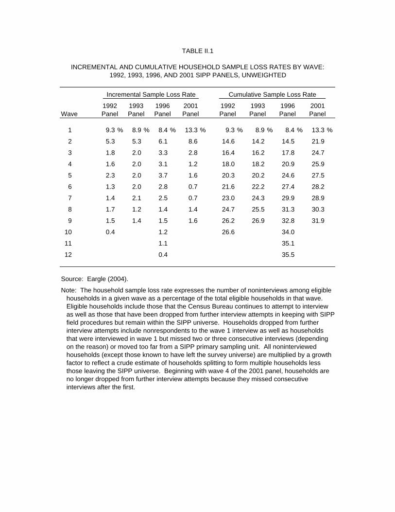
TABLE II.1

INCREMENTAL AND CUMULATIVE HOUSEHOLD SAMPLE LOSS RATES BY WAVE:1992, 1993, 1996, AND 2001 SIPP PANELS, UNWEIGHTED

Incremental Sample Loss Rate Cumulative Sample Loss Rate

1992 1993 1996 2001 1992 1993 1996 2001Wave Panel Panel Panel Panel Panel Panel Panel Panel

1 9.3 % 8.9 % 8.4 % 13.3 % 9.3 % 8.9 % 8.4 % 13.3 %

2 5.3 5.3 6.1 8.6 14.6 14.2 14.5 21.9

3 1.8 2.0 3.3 2.8 16.4 16.2 17.8 24.7

4 1.6 2.0 3.1 1.2 18.0 18.2 20.9 25.9

5 2.3 2.0 3.7 1.6 20.3 20.2 24.6 27.5

6 1.3 2.0 2.8 0.7 21.6 22.2 27.4 28.2

7 1.4 2.1 2.5 0.7 23.0 24.3 29.9 28.9

8 1.7 1.2 1.4 1.4 24.7 25.5 31.3 30.3

9 1.5 1.4 1.5 1.6 26.2 26.9 32.8 31.9

10 0.4 1.2 26.6 34.0

11 1.1 35.1

12 0.4 35.5

Source: Eargle (2004).

Note: The household sample loss rate expresses the number of noninterviews among eligible households in a given wave as a percentage of the total eligible households in that wave. Eligible households include those that the Census Bureau continues to attempt to interview as well as those that have been dropped from further interview attempts in keeping with SIPP field procedures but remain within the SIPP universe. Households dropped from further interview attempts include nonrespondents to the wave 1 interview as well as households that were interviewed in wave 1 but missed two or three consecutive interviews (depending on the reason) or moved too far from a SIPP primary sampling unit. All noninterviewed households (except those known to have left the survey universe) are multiplied by a growth factor to reflect a crude estimate of households splitting to form multiple households less those leaving the SIPP universe. Beginning with wave 4 of the 2001 panel, households are no longer dropped from further interview attempts because they missed consecutive interviews after the first.

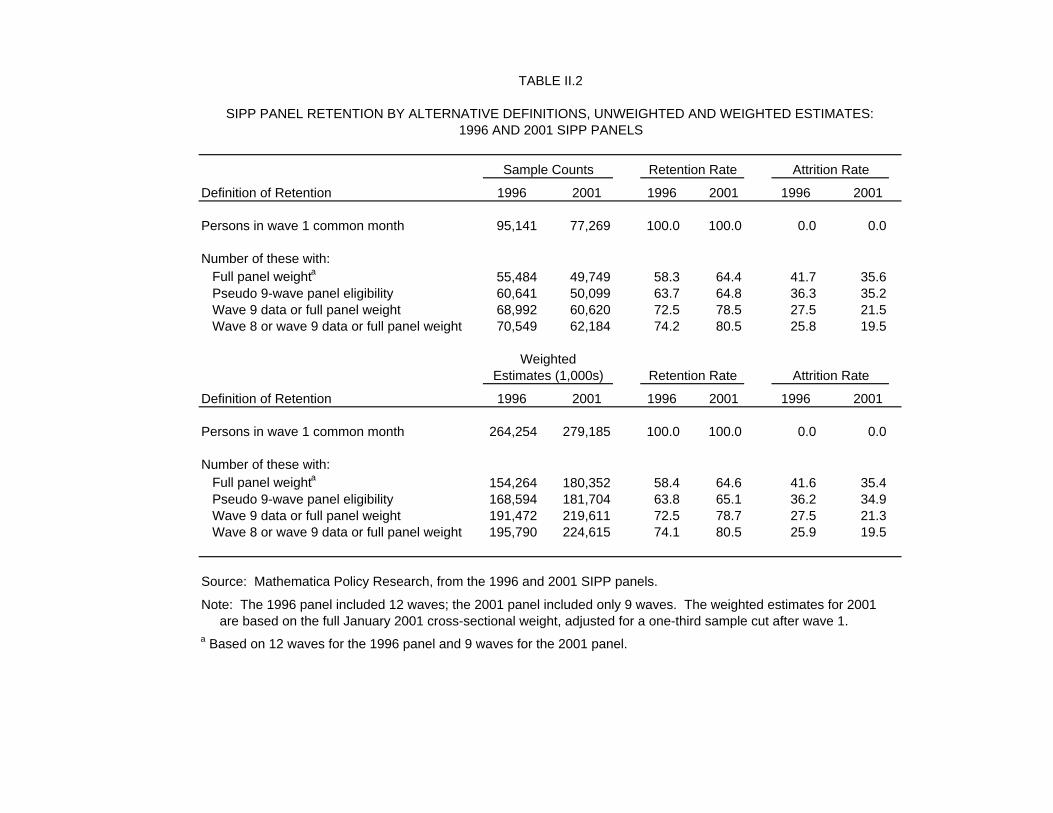
TABLE II.2

SIPP PANEL RETENTION BY ALTERNATIVE DEFINITIONS, UNWEIGHTED AND WEIGHTED ESTIMATES:1996 AND 2001 SIPP PANELS

Sample Counts Retention Rate Attrition Rate

Definition of Retention 1996 2001 1996 2001 1996 2001

Persons in wave 1 common month 95,141 77,269 100.0 100.0 0.0 0.0

Number of these with: Full panel weighta 55,484 49,749 58.3 64.4 41.7 35.6 Pseudo 9-wave panel eligibility 60,641 50,099 63.7 64.8 36.3 35.2 Wave 9 data or full panel weight 68,992 60,620 72.5 78.5 27.5 21.5 Wave 8 or wave 9 data or full panel weight 70,549 62,184 74.2 80.5 25.8 19.5

WeightedEstimates (1,000s) Retention Rate Attrition Rate

Definition of Retention 1996 2001 1996 2001 1996 2001

Persons in wave 1 common month 264,254 279,185 100.0 100.0 0.0 0.0

Number of these with: Full panel weighta 154,264 180,352 58.4 64.6 41.6 35.4 Pseudo 9-wave panel eligibility 168,594 181,704 63.8 65.1 36.2 34.9 Wave 9 data or full panel weight 191,472 219,611 72.5 78.7 27.5 21.3 Wave 8 or wave 9 data or full panel weight 195,790 224,615 74.1 80.5 25.9 19.5

Source: Mathematica Policy Research, from the 1996 and 2001 SIPP panels.

Note: The 1996 panel included 12 waves; the 2001 panel included only 9 waves. The weighted estimates for 2001 are based on the full January 2001 cross-sectional weight, adjusted for a one-third sample cut after wave 1.a Based on 12 waves for the 1996 panel and 9 waves for the 2001 panel.

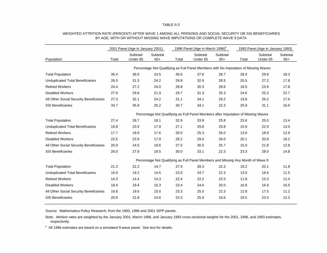
TABLE II-3

WEIGHTED ATTRITION RATE (PERCENT) AFTER WAVE 1 AMONG ALL PERSONS AND SOCIAL SECURITY OR SSI BENEFICIARIESBY AGE, WITH OR WITHOUT MISSING WAVE IMPUTATIONS OR COMPLETE WAVE 9 DATA

2001 Panel (Age in January 2001) 1996 Panel (Age in March 1996)a 1993 Panel (Age in January 1993)

Subtotal Subtotal Subtotal Subtotal Subtotal SubtotalPopulation Total Under 65 65+ Total Under 65 65+ Total Under 65 65+

Total Population 35.4 36.9 24.5 36.6 37.6 28.7 28.4 29.8 18.3

Unduplicated Total Beneficiaries 26.5 31.5 24.2 29.9 32.9 28.5 20.5 27.2 17.8

Retired Workers 24.4 27.2 24.0 28.8 30.3 28.6 18.5 23.9 17.8

Disabled Workers 27.9 29.8 21.9 29.7 31.3 25.3 24.6 25.3 22.7

All Other Social Security Beneficiaries 27.3 32.1 24.2 31.1 34.1 29.2 19.8 26.2 17.6

SSI Beneficiaries 33.7 35.9 26.2 30.7 34.1 22.3 25.9 31.1 16.6

Total Population 27.4 28.7 18.1 32.9 33.9 25.8 23.6 25.0 13.4

Unduplicated Total Beneficiaries 19.8 23.9 17.9 27.1 29.8 25.8 15.9 22.9 13.0

Retired Workers 17.7 18.9 17.6 26.0 25.3 26.0 13.6 18.9 12.9

Disabled Workers 22.5 23.9 17.9 28.2 29.0 26.0 20.1 20.8 18.2

All Other Social Security Beneficiaries 20.9 24.5 18.6 27.5 30.5 25.7 15.0 21.8 12.8

SSI Beneficiaries 26.0 27.9 19.5 30.0 33.1 22.3 23.3 28.0 14.8

Total Population 21.3 22.2 14.7 27.5 28.3 22.3 19.2 20.1 11.8

Unduplicated Total Beneficiaries 16.0 19.2 14.5 23.0 24.7 22.3 13.5 18.6 11.5

Retired Workers 14.3 14.4 14.3 22.4 22.2 22.5 11.8 15.3 11.4

Disabled Workers 18.4 19.4 15.3 23.4 24.6 20.0 16.8 16.9 16.5

All Other Social Security Beneficiaries 16.8 19.6 15.0 23.3 25.0 22.3 12.8 17.5 11.2

SSI Beneficiaries 20.9 22.8 14.6 23.3 25.9 16.6 19.5 23.5 12.2

Source: Mathematica Policy Research, from the 1993, 1996 and 2001 SIPP panels.

Note: Attrition rates are weighted by the January 2001, March 1996, and January 1993 cross-sectional weights for the 2001, 1996, and 1993 estimates, respectively.a All 1996 estimates are based on a simulated 9-wave panel. See text for details.

Percentage Not Qualifying as Full Panel Members after Imputation of Missing Waves

Percentage Not Qualifying as Full Panel Members and Missing Any Month of Wave 9

Percentage Not Qualifying as Full Panel Members with No Imputation of Missing Waves

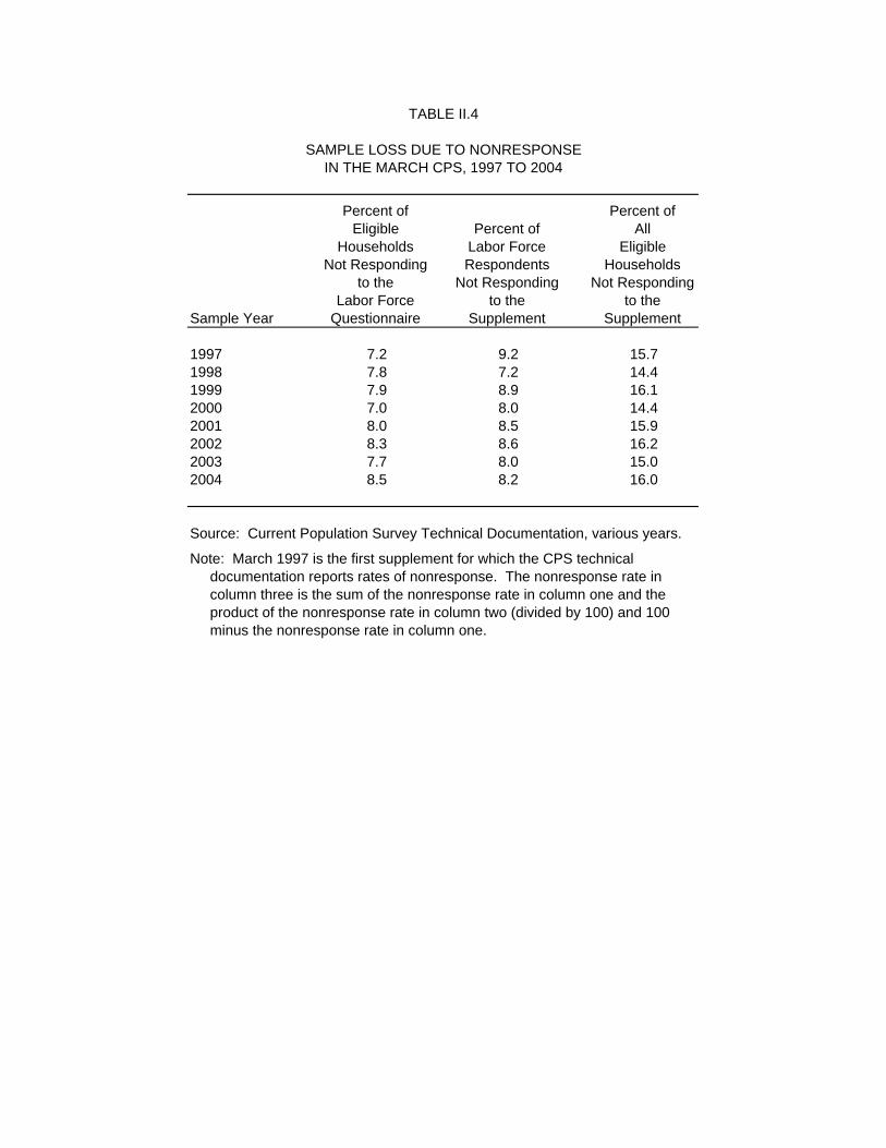
TABLE II.4

SAMPLE LOSS DUE TO NONRESPONSEIN THE MARCH CPS, 1997 TO 2004

Percent of Percent ofEligible Percent of All

Households Labor Force EligibleNot Responding Respondents Households

to the Not Responding Not RespondingLabor Force to the to the

Sample Year Questionnaire Supplement Supplement

1997 7.2 9.2 15.71998 7.8 7.2 14.41999 7.9 8.9 16.12000 7.0 8.0 14.42001 8.0 8.5 15.92002 8.3 8.6 16.22003 7.7 8.0 15.02004 8.5 8.2 16.0

Source: Current Population Survey Technical Documentation, various years.

Note: March 1997 is the first supplement for which the CPS technical documentation reports rates of nonresponse. The nonresponse rate in column three is the sum of the nonresponse rate in column one and the product of the nonresponse rate in column two (divided by 100) and 100 minus the nonresponse rate in column one.

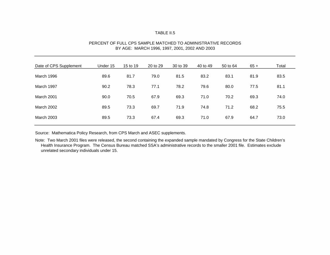
TABLE II.5

PERCENT OF FULL CPS SAMPLE MATCHED TO ADMINISTRATIVE RECORDSBY AGE: MARCH 1996, 1997, 2001, 2002 AND 2003

Date of CPS Supplement Under 15 15 to 19 20 to 29 30 to 39 40 to 49 50 to 64 65 + Total

March 1996 89.6 81.7 79.0 81.5 83.2 83.1 81.9 83.5

March 1997 90.2 78.3 77.1 78.2 79.6 80.0 77.5 81.1

March 2001 90.0 70.5 67.9 69.3 71.0 70.2 69.3 74.0

March 2002 89.5 73.3 69.7 71.9 74.8 71.2 68.2 75.5

March 2003 89.5 73.3 67.4 69.3 71.0 67.9 64.7 73.0

Source: Mathematica Policy Research, from CPS March and ASEC supplements.

Note: Two March 2001 files were released, the second containing the expanded sample mandated by Congress for the State Children’s Health Insurance Program. The Census Bureau matched SSA’s administrative records to the smaller 2001 file. Estimates exclude unrelated secondary individuals under 15.

TABLE II.6

PERCENT OF FULL CPS SAMPLE MATCHED TO ADMINISTRATIVE RECORDSBY RATIO OF FAMILY INCOME TO POVERTY AND AGE IN MARCH 2001

Family Income Relative toThe Federal Poverty Level Under 15 15 to 19 20 to 29 30 to 39 40 to 49 50 to 64 65 + Total

Under 10 percent 77.9 62.0 52.5 52.1 58.5 60.4 55.4 61.010 to under 50 percent 85.3 72.6 66.6 68.7 71.7 69.1 60.2 75.150 to under 100 percent 83.8 70.2 65.9 66.0 71.7 67.7 66.1 72.6100 to under 200 percent 87.9 67.8 68.3 67.4 69.6 68.2 68.0 73.4200 to under 300 percent 91.0 71.4 67.7 71.0 69.1 66.8 69.4 74.1300 to under 400 percent 93.3 71.4 69.7 70.2 71.8 70.2 69.7 75.2400 to under 600 percent 92.8 69.7 68.4 70.2 70.9 71.2 71.1 74.4600 percent or more 93.6 73.7 69.1 70.1 72.9 72.5 73.2 74.8

Total 90.0 70.5 67.9 69.3 71.0 70.2 69.3 74.0

Source: Mathematica Policy Research, from the 2001 CPS March supplement.

Note: Two March 2001 files were released, the second containing the expanded sample mandated by Congress for the State Children’s Health Insurance Program. The Census Bureau matched SSA’s administrative records to the smaller 2001 file. Estimates exclude unrelated secondary individuals under 15, for whom relative income is undefined.

TABLE II.7

PERCENT OF CPS SAMPLE MATCHED TO ADMINISTRATIVE RECORDS, BY RESPONSE TO THE CPS SUPPLEMENT AND AGE: MARCH 1996, 1997, 2001, AND 2002

Response to CPS SupplementAnd Date of Supplement Under 10 10 to 19 20 to 29 30 to 39 40 to 49 50 to 64 65 + Total

Respondents to the Supplement March 1996 90.6 87.6 81.7 84.3 86.0 86.0 84.8 85.9 March 1997 91.1 86.3 79.9 80.9 82.5 83.2 80.5 83.6 March 2001 91.3 82.4 71.1 72.5 74.2 73.1 71.6 76.7 March 2002 90.6 84.5 72.2 74.4 77.3 73.9 70.9 77.8

Nonrespondents to the Supplement March 1996 79.1 71.4 57.9 58.4 63.3 62.3 62.8 64.6 March 1997 78.0 68.3 54.0 54.7 56.8 56.7 51.4 59.5 March 2001 79.3 62.5 44.2 44.0 45.9 46.6 45.8 51.8 March 2002 78.6 65.2 50.1 50.6 53.4 47.8 43.6 54.9

Source: Mathematica Policy Research, from CPS March and ASEC supplements.

Note: Two March 2001 files were released, the second containing the expanded sample mandated by Congress for the State Children’s Health Insurance Program. The Census Bureau matched SSA’s administrative records to the smaller 2001 file. Estimates exclude unrelated secondary individuals under 15, for whom relative income is undefined.

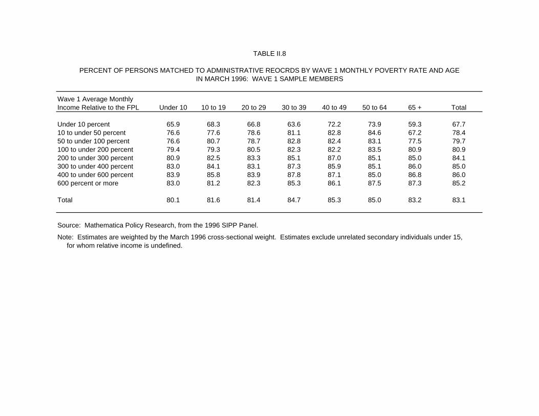
TABLE II.8

PERCENT OF PERSONS MATCHED TO ADMINISTRATIVE REOCRDS BY WAVE 1 MONTHLY POVERTY RATE AND AGEIN MARCH 1996: WAVE 1 SAMPLE MEMBERS

Wave 1 Average MonthlyIncome Relative to the FPL Under 10 10 to 19 20 to 29 30 to 39 40 to 49 50 to 64 65 + Total

Under 10 percent 65.9 68.3 66.8 63.6 72.2 73.9 59.3 67.710 to under 50 percent 76.6 77.6 78.6 81.1 82.8 84.6 67.2 78.450 to under 100 percent 76.6 80.7 78.7 82.8 82.4 83.1 77.5 79.7100 to under 200 percent 79.4 79.3 80.5 82.3 82.2 83.5 80.9 80.9200 to under 300 percent 80.9 82.5 83.3 85.1 87.0 85.1 85.0 84.1300 to under 400 percent 83.0 84.1 83.1 87.3 85.9 85.1 86.0 85.0400 to under 600 percent 83.9 85.8 83.9 87.8 87.1 85.0 86.8 86.0600 percent or more 83.0 81.2 82.3 85.3 86.1 87.5 87.3 85.2

Total 80.1 81.6 81.4 84.7 85.3 85.0 83.2 83.1

Source: Mathematica Policy Research, from the 1996 SIPP Panel.

Note: Estimates are weighted by the March 1996 cross-sectional weight. Estimates exclude unrelated secondary individuals under 15, for whom relative income is undefined.

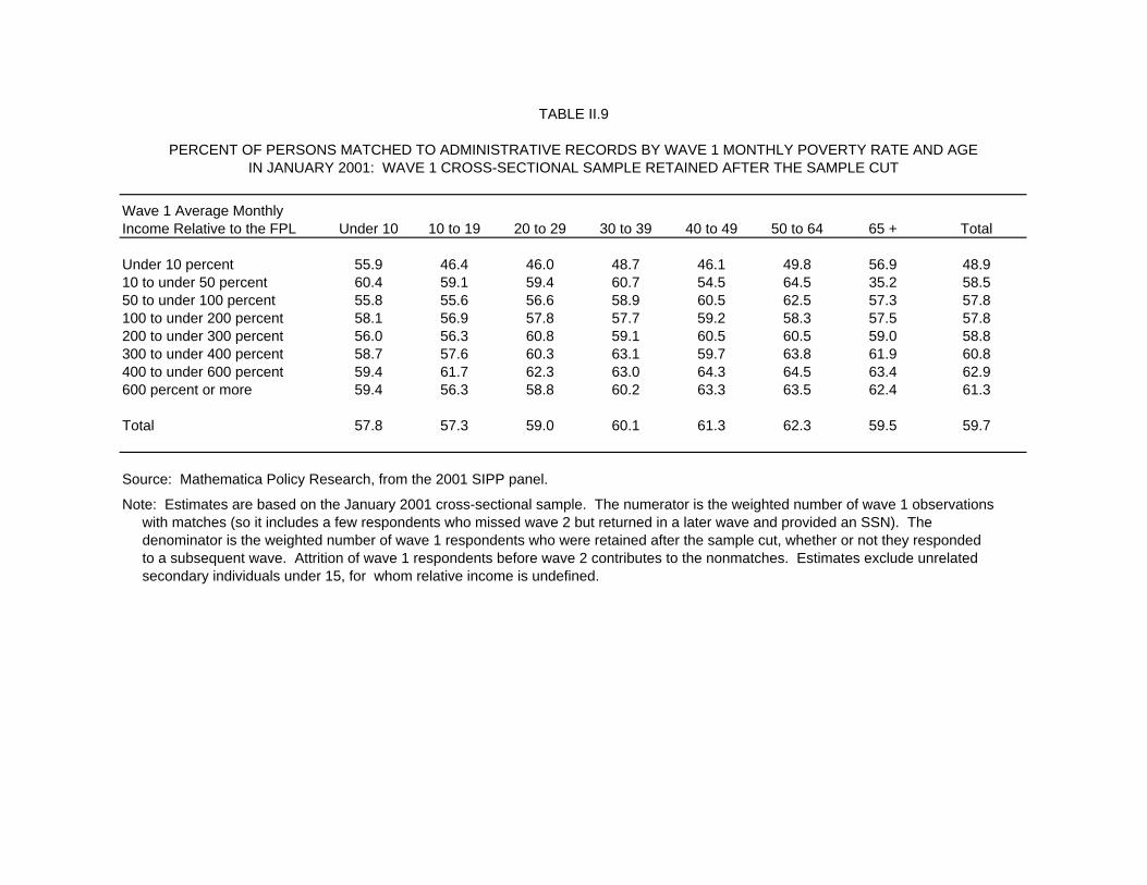
TABLE II.9

PERCENT OF PERSONS MATCHED TO ADMINISTRATIVE RECORDS BY WAVE 1 MONTHLY POVERTY RATE AND AGEIN JANUARY 2001: WAVE 1 CROSS-SECTIONAL SAMPLE RETAINED AFTER THE SAMPLE CUT

Wave 1 Average MonthlyIncome Relative to the FPL Under 10 10 to 19 20 to 29 30 to 39 40 to 49 50 to 64 65 + Total

Under 10 percent 55.9 46.4 46.0 48.7 46.1 49.8 56.9 48.910 to under 50 percent 60.4 59.1 59.4 60.7 54.5 64.5 35.2 58.550 to under 100 percent 55.8 55.6 56.6 58.9 60.5 62.5 57.3 57.8100 to under 200 percent 58.1 56.9 57.8 57.7 59.2 58.3 57.5 57.8200 to under 300 percent 56.0 56.3 60.8 59.1 60.5 60.5 59.0 58.8300 to under 400 percent 58.7 57.6 60.3 63.1 59.7 63.8 61.9 60.8400 to under 600 percent 59.4 61.7 62.3 63.0 64.3 64.5 63.4 62.9600 percent or more 59.4 56.3 58.8 60.2 63.3 63.5 62.4 61.3

Total 57.8 57.3 59.0 60.1 61.3 62.3 59.5 59.7

Source: Mathematica Policy Research, from the 2001 SIPP panel.

Note: Estimates are based on the January 2001 cross-sectional sample. The numerator is the weighted number of wave 1 observations with matches (so it includes a few respondents who missed wave 2 but returned in a later wave and provided an SSN). The denominator is the weighted number of wave 1 respondents who were retained after the sample cut, whether or not they responded to a subsequent wave. Attrition of wave 1 respondents before wave 2 contributes to the nonmatches. Estimates exclude unrelated secondary individuals under 15, for whom relative income is undefined.

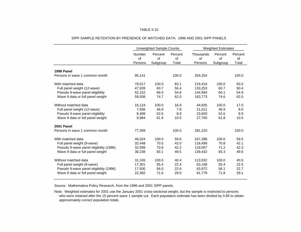
TABLE II.10

SIPP SAMPLE RETENTION BY PRESENCE OF MATCHED DATA: 1996 AND 2001 SIPP PANELS

Unweighted Sample Counts Weighted Estimates

Number Percent Percent Thousands Percent Percentof of of of of of

Persons Subgroup Total Persons Subgroup Total

1996 PanelPersons in wave 1 common month 95,141 100.0 264,254 100.0

With matched data 79,017 100.0 83.1 219,419 100.0 83.0 Full panel weight (12-wave) 47,928 60.7 50.4 133,253 60.7 50.4 Pseudo 9-wave panel eligibility 52,152 66.0 54.8 144,994 66.1 54.9 Wave 9 data or full panel weight 59,008 74.7 62.0 163,773 74.6 62.0

Without matched data 16,124 100.0 16.9 44,835 100.0 17.0 Full panel weight (12-wave) 7,556 46.9 7.9 21,011 46.9 8.0 Pseudo 9-wave panel eligibility 8,489 52.6 8.9 23,600 52.6 8.9 Wave 9 data or full panel weight 9,984 61.9 10.5 27,700 61.8 10.5

2001 PanelPersons in wave 1 common month 77,269 100.0 281,220 100.0

With matched data 46,024 100.0 59.6 167,288 100.0 59.5 Full panel weight (9-wave) 32,448 70.5 42.0 118,499 70.8 42.1 Pseudo 9-wave panel eligibility (1996) 32,599 70.8 42.2 119,057 71.2 42.3 Wave 9 data or full panel weight 38,238 83.1 49.5 139,432 83.3 49.6

Without matched data 31,245 100.0 40.4 113,932 100.0 40.5 Full panel weight (9-wave) 17,301 55.4 22.4 63,168 55.4 22.5 Pseudo 9-wave panel eligibility (1996) 17,500 56.0 22.6 63,972 56.1 22.7 Wave 9 data or full panel weight 22,382 71.6 29.0 81,779 71.8 29.1

Source: Mathematica Policy Research, from the 1996 and 2001 SIPP panels.

Note: Weighted estimates for 2001 use the January 2001 cross-sectional weight, but the sample is restricted to persons who were retained after the 15 percent wave 1 sample cut. Each population estimate has been divided by 0.85 to obtain approximately correct population totals.

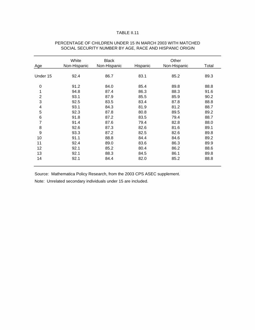
TABLE II.11

PERCENTAGE OF CHILDREN UNDER 15 IN MARCH 2003 WITH MATCHEDSOCIAL SECURITY NUMBER BY AGE, RACE AND HISPANIC ORIGIN

White Black OtherAge Non-Hispanic Non-Hispanic Hispanic Non-Hispanic Total

Under 15 92.4 86.7 83.1 85.2 89.3

0 91.2 84.0 85.4 89.8 88.81 94.8 87.4 86.3 88.3 91.62 93.1 87.9 85.5 85.9 90.23 92.5 83.5 83.4 87.8 88.84 93.1 84.3 81.9 81.2 88.75 92.3 87.8 80.8 89.5 89.26 91.8 87.2 83.5 79.4 88.77 91.4 87.6 79.4 82.8 88.08 92.6 87.3 82.6 81.6 89.19 93.3 87.2 82.5 82.6 89.8

10 91.1 88.8 84.4 84.6 89.211 92.4 89.0 83.6 86.3 89.912 92.1 85.2 80.4 86.2 88.613 92.1 88.3 84.5 86.1 89.814 92.1 84.4 82.0 85.2 88.8

Source: Mathematica Policy Research, from the 2003 CPS ASEC supplement.

Note: Unrelated secondary individuals under 15 are included.

41

III. MATCH BIAS IN THE SIPP AND CPS

The matching of administrative records to the SIPP not only enhances the quality and

analytical utility of SIPP and CPS data; it provides an especially powerful tool for evaluating the

bias introduced into SIPP data by attrition. Declining match rates between survey records and

administrative records, documented in the preceding chapter, raise concerns about the continued

representativeness of matched samples from both the SIPP and the CPS. While the Census

Bureau has taken steps that will restore match rates to levels that have not been seen for years,

these improvements will not benefit SIPP or CPS data collected prior to 2006. The findings

presented in Chapter II make clear that recent declines in match rates in both surveys, but

particularly the SIPP, are more significant than growth in attrition in the SIPP. Furthermore,

before we can assess the impact of the sample loss that accompanies attrition, we need to

establish whether matched records provide a biased picture of the population that they are

intended to represent. For these reasons we take up matching bias before we turn to attrition

bias. This chapter examines evidence of match bias in both the SIPP and the CPS. We begin

with a discussion of how we approach the evaluation of match bias and then turn to empirical

findings for the two surveys.

A. EVALUATING MATCH BIAS

We confront a fundamental problem in our attempt to evaluate the magnitude of bias due to

nonmatching—namely, we do not know which members of a survey sample are actually

included in the administrative data and, therefore, should match. Thus we do not know what

match rate we would observe if all of the survey records represented in the administrative data

could be matched; nor do we know how the sample members for whom administrative data exist

differ from those for whom it does not. This is important because we have every reason to

42

believe that the sample members who are not included in the administrative records of SSA are

systematically different from the sample members who are included. We can speculate that the

people who are “outside the system,” so to speak, tend to be disproportionately low-income,

young and members of minorities, and that many are recent immigrants who lack citizenship.

Nearly all citizens of the U.S. should have SSNs, given tax law requirements implemented

in the 1980s. A very substantial proportion of the infants born in the United States receive SSNs

through the birth registration system, under a cooperative arrangement between SSA and the

states. In March 2001, an estimated 6.7 percent of the CPS universe (and, therefore, the SIPP

universe as well) was foreign born and not citizens of the United States. Citizenship is not a

requirement for obtaining an SSN. SSNs are issued to noncitizens allowed to work in the U.S.,

for example. But to obtain SSNs noncitizens must provide legal documentation of their

immigration status. This leaves undocumented aliens as the largest group of persons without

SSNs—or without their own SSNs and, therefore, not likely to match to SSA’s database of

SSNs. A recent estimate places the number of undocumented aliens at 11.5 to 12 million or

about 4 percent of the U.S. population (Passel 2006).

Other foreign nationals who are in the country temporarily and earning income that is

taxable under U.S. law may be required to obtain individual taxpayer identification numbers

(ITINs) in lieu of SSNs. These ITINs are issued by the Treasury Department. They resemble

SSNs in form, but they always have nine digits and begin with the number 9, which puts them

outside the range of numbers reserved for SSNs. Persons who file tax returns with ITINs will be

included in the IRS’s database of tax returns and information documents (W-2s, 1099s and the

like), but because their ITINs are not SSNs, we do not believe that they are included in the

records that SSA links to the SIPP and the CPS. The IRS has estimated that in the 2004 tax year

the number of ITINs appearing on tax returns as filers or dependents or as nonfilers with

43

information documents was 5.0 million, which is just under 2 percent of the civilian

noninstitutional population.1

Drawing inferences from matched data to the broader universe that these data represent is

hampered by our inability to identify and characterize that broader universe empirically. Not

knowing what fraction of a survey sample should match to SSA’s administrative records, we

cannot determine how complete is the match for any one survey. The estimates cited above

provide some help. Putting together the estimates of undocumented aliens and the subset of

documented aliens with ITINs instead of SSNs suggests that these groups account for nearly 6

percent of the population. This implies that 94 percent of the population is covered by SSNs and

ought to be represented in SSA’s administrative records.

While the source of bias in matched samples is the difference between matched records and

nonmatched records, the bias that we want to evaluate is the difference between the matched

subsample and the full sample, as the matched subsample is what will be used in any analysis.

For such a comparison the match rate matters. The higher the match rate, the less important are

differences between matched and unmatched records. This is analogous to survey response

rates, where the overall bias is a function of both the response rate and how much the

nonrespondents differ from the respondents. Because the match rate plunged between the 1996

and 2001 SIPP panels, SSA needs an estimate of match bias that is sensitive to the match rate.

To evaluate bias in the matched subsample, we first calibrated the matched subsample to the

same demographic controls to which the Census Bureau had calibrated the full cross-sectional

sample.2 These controls include a cross-classification of sex, detailed age, and race (black versus

1 The Statistics of Income Division of the IRS prepared this estimate from its annual sample of tax returns

combined with information documents.

2 The calibration methodology is documented in Appendix A, and MPR’s calibration programs are being delivered as part of this report. Calibration is the final operation in assigning sample weights. The Census Bureau’s

44

nonblack); a more limited cross-classification of sex by Hispanic origin and broad age group;

and relationship to the householder, by sex and race. Since match rates are known to differ

across demographic subgroups, any use of a matched subsample would have to include some

form of adjustment to compensate for such differences. Calibrating the matched records to the

same population controls used by the Census Bureau is a fundamental first step. It represents the

minimum adjustment that we would want to apply to matched data before evaluating their bias.

If serious biases are identified, then we would want to develop additional adjustments targeting

these biases and then re-evaluate the matched subsample with these new adjustments.

We compared the calibrated matched subsample and the full sample with respect to a wide

variety of personal, family and household characteristics as well as the results of several

illustrative applications of matched data specified by SSA. Ideally, we would want to compare

the matched subsample to what might be termed the “fully matched” subsample, in which every

sample record with a corresponding administrative record was identified.3 Some of the records

in the survey sample do not have corresponding administrative records, and, as we have noted,

there is good reason to believe that these records differ systematically from the matched records.

By comparing our matched subsample to the full survey sample, we risk misinterpreting

systematic differences between records that do or do not have representation in the

administrative databases as bias in the matching process (or, more specifically, bias in the

reporting of correct SSNs). This problem is unavoidable when we attempt to evaluate match bias

(continued) weighting procedures also include steps designed to equalize the weights of spouses. We did not include those steps in our calibration of the matched subsample because spouses will not necessarily both be matched. Similarly, when we calibrate a matched sample of panel records, as was done for the analyses presented in the next chapter, we do not attempt to equalize the weights of spouses because they may not both have full panel weights.

3 In addition to excluding sample members without SSNs from the total population, we would like to be able to calibrate our matched samples to population controls that exclude persons without SSNs. Since neither is possible, we calibrate our matched samples to controls that reflect the total population, and we compare the calibrated matched sample to the total sample.

45

with respect to estimates of the total population. When we restrict our comparisons to self-

reported SSA beneficiaries, however, we would expect that any sample members who are not

represented in the SSA administrative databases are largely if not entirely excluded.

For the SIPP evaluation, we calculated standard errors using replicate weights provided by

the Census Bureau. The Census Bureau’s replicate weights incorporate sample design

information that is not released on the public use file, so these weights enable the external user to

calculate truer standard errors than is possible with any other method. Furthermore, with

replicate weights we can directly estimate the standard error of a difference between an estimate

based on a subsample (namely, matched records) and an estimate based on the full sample from

which the subsample was taken (matched plus unmatched records). The Census Bureau has

produced a set of replicate weights for every SIPP weight, both cross-sectional and longitudinal.

To use the Bureau’s replicate weights for our various reweightings of matched records, we

recalibrated both the sample weights and the associated replicate weights for the matched

records. The calibration procedures are detailed in Appendix A. The estimation of standard

errors is discussed in Appendix B.

B. MATCH BIAS IN THE SIPP

From SSA’s perspective, the most important questions about match bias involve the impact

of the low match rate in the 2001 panel. How does the low match rate documented in the

previous chapter affect potential uses of matched SIPP and administrative data? Can matched

records adequately represent the subpopulations from which they are drawn? What adjustments

to survey weights are required, and what are their limits? More generally, what accommodation

must be made in using the matched data for analysis? Are the potential benefits worth the effort,

or should SSA bypass the 2001 panel altogether?

46

We address these questions by comparing matched and full sample estimates over a variety

of potential applications. SSA uses matched SIPP and administrative records in applications that

take advantage of the longitudinal design of the SIPP as well as in strictly cross-sectional,

descriptive studies. In our assessment of match bias in the 2001 panel we begin by comparing

matched and full sample estimates of a wide range of characteristics for the total population and

for subpopulations of SSA beneficiaries. Then we evaluate match bias in estimates of eligibility

for SSI—an application of matched data that SSA asked us to include. We compare matched

and full sample estimates of income and asset eligibility at multiple points in time using both the

1996 and 2001 SIPP panels. The comparisons include calendar year longitudinal estimates of

month-to-month fluctuation in income eligibility. Lastly, we examine the magnitude of match

bias in estimates of the pension coverage of divorced women, another application identified by

SSA and one that uses longitudinal data spanning six waves and two topical modules.

1. Comparison of Matched Respondents and All Respondents in the 2001 Panel

One consequence of the Census Bureau’s moving the request for SSNs from the first wave

to the second wave of the 2001 panel, besides the steep drop in SSNs collected, is that sample

members who attrited between waves 1 and 2 can have no matched data. Therefore, any

comparison of matched and full sample records that includes wave 1 attriters in the full sample

will confound match bias with attrition bias. For this reason, we designed our comparisons to

exclude wave 1 attriters. Specifically, we compared matched and full sample records within the

following subsamples: (1) wave 1 respondents who also responded to all four months of wave 2;

(2) respondents to wave 2, which includes not only the wave 1/wave 2 respondents but those

additional persons who joined sample households in wave 2 (all of whom were asked for their

SSNs); and (3) full panel sample members, who exclude all attriters as well as those who missed

only an occasional wave. The wave 1/wave 2 respondents were compared with respect to their

47

wave 1 characteristics. The wave 2 respondents were compared with respect to their wave 2

characteristics, including topical module data on immigration and citizenship, which were

collected only in wave 2. The full panel sample members were compared with respect to both

wave 1 and wave 9 characteristics. All of these comparisons were repeated for the 1996 panel so

that we could assess whether match bias increased between the two panels.

For each subsample we compared matched respondents and all respondents in the total

population and four subpopulations of SSA beneficiaries: (1) retired workers, (2) disabled

workers, (3) other Social Security recipients, and (4) SSI recipients. Comparisons were made

with respect to a number of personal, family, and household demographic and economic

characteristics, by age, using age groups that were specific to each subpopulation. Appendix C

contains the results of one set of comparisons, for wave1/wave2 respondents from the 2001

panel. Each table is laid out as follows. The first four columns present full wave 1/wave 2

sample estimates for all persons and three age groups. The next four columns present differences

between the matched subsample and full sample estimates, with indicators of statistical

significance.

There are 20 tables in all. Table C.1.a compares the calibrated matched and full samples

with respect to estimates of the distribution of personal demographic characteristics for the total

population. Tables C.1.b through C.1.e repeat these comparisons for the four beneficiary

subpopulations. Tables C.2.a through C.2.e provide comparisons for health insurance coverage

and personal income. Tables C.3.a through C.3.e provide comparisons with respect to household

and family composition and home ownership, and Tables C.4.a through C.4.e present

comparisons for household and family economic characteristics.

Looking past statistical significance for the moment, we find that the overwhelming

impression that emerges from the 20 pages of comparisons is that the reweighted matched

48

sample represents the reweighted full sample, exclusive of wave 1 attriters, exceedingly well.

The similarities are striking, especially when we consider that, overall, the matched wave 1/wave

2 sample includes only 63 percent of the full wave 1/wave 2 sample. Calibrating both samples to

the SIPP population controls appears to have eliminated, in large part, whatever differences may

exist between all wave 1/wave 2 respondents and those who could be matched to administrative

records.

As small as they are, many of the differences between the matched and full sample estimates

of the total population are statistically significant. Whether this is due to the small population of

persons who have no administrative records and, therefore, are represented only by the full

sample, or whether it reflects true but very small differences between matched and full sample

cases that do have administrative records cannot be resolved with these data. For the four SSA

beneficiary subpopulations we find larger differences than for the total population. We attribute

the greater magnitudes of these differences to the smaller sample sizes, and, indeed, few of these

differences are statistically significant. Moreover, the beneficiary subpopulations presumably

exclude persons without SSA administrative records, which would eliminate a potential

difference between the matched and full samples that is present for the total population. Because

of their smaller sample sizes, however, we are not able to say that the beneficiary subpopulations

do indeed show smaller biases. In fact, for the retired worker population, we find some evidence

of a lesser reliance on Social Security benefits and greater family income—both absolute and

relative to poverty—within the matched versus full sample (see Tables C.2.b and C.4.b). We call

attention to this possible evidence of a slight bias in the matched beneficiary population because

it is repeated in the CPS, as we show later in the chapter. But even here the differences involve

deviations that do not exceed 2 percentage points in any income category, and most are a good

deal smaller than that.

49

We can examine the possible impact of sample members without SSA administrative

records more directly by looking at the citizenship and migration data collected in the wave 2

topical module. Table III.1 compares the matched and full sample estimates of the distribution

of selected characteristics for the total population. Not surprisingly, matched respondents are

more likely than all respondents to be native-born citizens, but the difference is only 2

percentage points (89.1 versus 87.3). Matched respondents are also less likely than all

respondents to be non-citizens, whether permanent residents (4.7 versus 5.3 percent again) or not

(1.5 versus 2.1). At the same time, however, matched respondents are actually less likely than

all respondents to be foreign-born U.S. citizens (4.7 versus 5.3), which would not reflect the

presence or absence of SSNs. All of these differences are statistically significant. Matched

respondents are also slightly less likely to have moved to the U.S. after 1990 (3.3 versus 3.9

percent), but they are more likely to have moved to their current residence within the previous

two years (20.5 versus 20.0 percent). None of these differences is particularly striking, given

that the characteristics that we are comparing are the most obvious ways in which people who

are not in the SSA administrative record system might be expected to differ from those who are

in the system.

If most of the wave 1 demographic and economic characteristics that we examined showed

little differentiation between the matched and full samples in the 2001 panel, then the steep

decline in the match rate between the 1996 and 2001 panels could not have had much effect on

match bias. This inference is confirmed in Appendices D and E, which compare the differences

between the matched and full samples in the 1996 and 2001 panels. Appendix D presents side

by side the differences in wave 1 characteristics between the matched and full wave 1/wave 2

samples in both panels. Appendix E does the same with the matched full panel and entire full

panel samples from the two panels. Certainly, the differences estimated from the 2001 panel are

50

more variable than those from the 1996 panel, given that the matched samples in 2001 are barely

half the size of those in the 1996 panel. Fewer differences in the 2001 panel are statistically

significant, even though they are often larger than those in the 1996 panel. But, again, even

when the differences are statistically significant, they are substantively unimportant for the most

part. Consider, for example, Social Security payments as a percentage of total personal income

among retired workers (Table D.2.b). The differences may be somewhat larger in the 2001

panel, and the largest differences are statistically significant, but the 2001 panel shows only

narrowly more evidence of bias than the 1996 panel, and the differences between the matched

and full samples lie within a range that we would characterize as small. In the same table, at the

top, we see clear evidence of smaller differences in health insurance coverage in the 2001 panel

among all retired workers and those under 65. Matched sample members in 2001 are clearly no

more likely than all sample members to own their own homes (Table D.3.a), and differences in

household and family income are negligible and clearly no greater in 2001 than 1996 (Table

D.4.a).

Differences between the matched full panel and entire full panel samples tell the same story.

Variability is greater in 2001, but there is little indication that the matched sample in 2001 is any

less representative of the full sample than in 1996. This is particularly clear in comparisons

involving income for the total population (Tables E.2.a and E.4.a) and retired workers (Tables

E.2.b and E.4.b). We also compared the matched and full panel samples with respect to

characteristics measured at wave 9 and reached the same conclusions (data not shown).

2. Eligibility for SSI

One of the key uses of SIPP by SSA as well as a number of other federal agencies and their

contractors is to estimate eligibility for entitlement and other assistance programs in a specific

month or series of months. In addition to monthly family composition and other variables that

51

condition eligibility, SIPP provides monthly estimates of income by source, which is needed to

calculate “countable” income under each program’s eligibility rules. SIPP also provides periodic

estimates of assets by type—generally, once a year. With these data it is possible to simulate

both income and asset eligibility during a number of specific months over the life of a SIPP

panel. It is also possible to simulate month-to-month changes in income-eligibility, as the

estimates of income, unlike assets, can change from month to month. (Monthly eligibility may

also be affected by changes in family composition, with or without attendant changes in income.)

SSA expressed an interest in both types of eligibility simulations for the SSI program.

Because it is exceedingly useful to link program administrative data—with monthly participation

and benefits paid—to monthly survey-based estimates of eligibility, these two eligibility

simulations provided good examples for evaluating bias in the matched samples.

a. Financial Eligibility in Selected Months

Financial eligibility for SSI among elderly persons was simulated in each of the SIPP waves

that collects asset data in its topical module. These are waves 3, 6, and 9 of both the 1996 and

2001 panels.4 We simulated eligibility for the calendar month that was common to the four

rotation groups in each wave. For the 1996 panel this meant November of 1996, 1997, and 1999,

and for the 2001 panel this meant September of 2001, 2002, and 2003. Estimates for the three

months from the 1996 panel are presented in Tables III.2a through III.2c. Estimates for the 2001

panel are presented in Tables III.3a through III.3c. Separate estimates are presented for the

percentage of persons simulated to be income eligible but not necessarily asset eligible (columns

1 and 2) and the percentage of persons who were both income and asset eligible (columns 3 and

4). The final two columns report estimates of the numbers of persons simulated to be income

4 The 1996 panel also collected asset data in wave 12 whereas the 2001 panel ended at wave 9. We limited our

evaluation to the common waves.

52

and asset eligible, with indicators of statistical significance for the differences between the

matched and full sample estimates.

For each year of the 1996 panel we find only small differences for both measures. In

general, we find slightly fewer eligibles with the matched subsample than the full cross-sectional

sample in each month. For example, 10.6 percent of the matched subsample is simulated to be

income eligible in November 1996, and 6.1 percent is simulated to be income and asset eligible.

The corresponding estimates from the full sample are 11.1 percent and 6.3 percent, respectively.

The difference in the estimated numbers of eligibles is statistically significant but very small—

about 74,000 from estimates of 1.955 versus 2.019 million. For non-Hispanic whites, the largest

subgroup reported, these differences run only 0.1 to 0.2 percentage points except for income

eligibility in 1998. The differences are consistently larger—about 1 percentage point—for non-

Hispanic nonwhites and for Hispanic persons. When we divide the elderly by age at 75 and look

separately at married versus single men and women, virtually all of the differences are under a

percentage point, and they mostly show fewer eligibles in the matched subsample. The one

consistent exception is among single men 65 to 74, where we find more income and asset

eligible persons in the matched subsample than in the full sample in each of the three months.

When we look at eligibility rates by the level of monthly income relative to poverty, we find

two patterns consistently across the three months. First, there are numerically more eligibles

below 50 percent of poverty in the full sample than in the matched subsample. This is true even

in September 2002 when the matched sample members in this lowest income category have a

higher eligibility rate (62.4 percent versus 54.3 percent). It is apparent from this that there are

more very low income people in the full sample than the matched sample. Second, the eligibility

rate among persons between 50 and 100 percent of poverty is consistently very slightly higher in

the matched subsample than the full sample. At higher income levels, where the difference

53

between countable income and total income explains much of simulated eligibility, the matched

and full samples vary with respect to which has the higher eligibility rate and the higher number

of eligibles.

It is important to point out that our eligibility simulation does not take account of

immigration status, which could bias the results in the direction of finding more eligibles in the

full sample than in the matched sample—which is exactly what we find overall.5 Undocumented

aliens, in particular, are likely to include a higher proportion of persons who meet the SSI

income and asset eligibility criteria. This will boost the simulated eligibility rates in the full

population compared to the matched subpopulation, even though many of these additional

“eligibles” would be ineligible because of their immigration status. While the young age

distribution of immigrants implies that people without SSNs make up a smaller share of the

elderly population than the nonelderly population, there may still be a sufficient number of

elderly persons without SSNs to explain the slightly higher estimated SSI eligibility rate in the

full sample versus the matched subsample. Taking this into account, it is quite possible that,

despite the lower estimates of SSI eligibility, the matched sample provides an accurate

representation of eligibility among elderly persons with SSNs.

Turning to the 2001 panel, we find, first, that for the elderly population as a whole, our

results are very similar to the 1996 panel. The matched sample has a slightly lower percentage

of income-eligibles and combined income and asset eligibles and numerically more of the latter

in all three months (Tables III.3a to III.3c). The middle month shows more of a spread in the

2001 panel than the 1996 panel, but the results in the first and third months are strikingly similar

between the two panels. For instance, in September 2003 the difference between the matched

5 The SIPP collects data on citizenship and migration history in the wave 2 topical module, but these data are

not updated in later waves, so changes in status are not recorded. For this reason, we elected not to include this information in our eligibility simulation.

54

and full sample estimates of the percentage of elderly persons income eligible for SSI is 0.3

percentage points versus 0.4 percentage points in November 1998. The difference between the

matched and full sample estimates of the percentage of elderly persons who were both income

and asset eligible for SSI is 0.2 percentage points in September 2003 versus 0.3 percentage

points in November 1998. The difference between the matched and full sample estimates of total

elderly persons eligible for SSI is less than 80,000 in September 2003 and 90,000 in November

1998.

Given the similarity of the findings for the nonelderly population as a whole, we would not

expect to find any notable differences between the two panels when we compare simulated

eligibility rates for subgroups of the nonelderly population. The findings support this

expectation. In fact, because of the greater sampling variability in the 2001 panel, which has

barely half as many matched cases as the 1996 panel, the matched sample yields a higher

subgroup eligibility rate than the full sample more often than it does in 1996. Among Hispanic

persons this may reflect more than sampling variability, although we have no other explanation.

In every one of the three months from the 2001 panel, the matched subsample yields higher

simulated eligibility rates for Hispanic persons and numerically more Hispanic eligibles than the

full sample.

b. Fluctuation in Monthly Income Eligibility

In comparisons based on calendar year data for 1997, 2001, and 2002, we find small but

systematic differences between the matched and full samples with respect to the proportion of

the elderly population that was ever income-eligible for SSI during a 12 month period and the

proportion that was eligible for six months or more (Tables III.4, III.5a and III.5b). Slightly

fewer of the matched cases were ever eligible during the year. For example, in 1997, 15.0

percent of the matched sample and 15.6 percent of the full sample was ever eligible for SSI.

55

Similarly, in 2002, 13.7 percent of the matched sample and 14.3 percent of the full sample was

ever eligible for SSI. We also find that, compared to the full sample, consistently smaller

proportions of the matched sample were eligible in January of each year and lost eligibility

during the year. In 1997, for example, 10.6 of the matched sample and 11.2 percent of the full

sample was eligible in January while 3.8 percent of the matched sample and 4.6 percent of the

full sample lost eligibility during the year. We find similar patterns in 2001 and 2002.

At the same time, however, we find no difference in any of the years between the matched

and full samples in the proportion of persons who were ineligible in January but became eligible

during the year. In 1997, 4.4 percent of the elderly in each sample became income eligible for

SSI during the year. In 2001, 5.7 percent of each sample became eligible during the year, and in

2002 4.1 percent of the matched subsample and 4.2 percent of the full sample became eligible

during the year.

To sum up, this examination of fluctuation in monthly income eligibility for SSI provides

further evidence that the substantially lower match rate in the 2001 panel had no impact on how

well the matched sample represents the full sample. Even where we found that the matched

sample differed systematically, albeit slightly, from the full sample, the magnitudes of the

differences were very consistent between the 1996 and 2001 panels. Furthermore, as with the

cross-sectional estimates presented earlier, these small differences between the matched and full

samples in longitudinal estimates of income eligibility for SSI could very well be due to low-

income immigrants without SSNs, who would be represented in the full sample but not the

matched subsample.

3. Pension Coverage of Divorced Women

Another illustrative application of matched SIPP data identified by SSA involves the impact

of a feature of the Social Security regulations that confers a spouse benefit on women who were

56

divorced from their former spouses after 10 years of marriage. Divorced women who were

married long enough to benefit from this provision may behave differently with respect to their

own pension coverage, receipt of Social Security benefits, or employment, and they may be

better off economically than divorced women who were married too few years to any one spouse

to have access to spouse benefits. To investigate this question requires marital history data

collected in wave 2 and pension coverage collected in wave 7, so only the full panel sample is

appropriate—that is, persons with data for all waves and assigned a full panel weight. The

subset of the full panel sample with matched data could be used for this analysis as well, so that

the richer and more accurate administrative data on Social Security recipiency could be

substituted for what is reported in the SIPP. We use this policy application to extend our

evaluation of bias in the matched subsample of the full panel relative to the entire full panel

sample.

Current marital status and age may have important effects on the outcome measures that are

of interest to SSA, so it is important to take these characteristics into account when examining

the impact of the length of a prior marriage that ended in divorce. The upper half of Table III.6

provides estimates of the distribution of women 50 and older with at least one divorce by age,

current marital status, and whether they were married to a divorced spouse for at least 10 years.

The lower half provides estimates of the difference between the matched full panel estimate and

the entire full panel estimate (matched minus full). Among women with at least one divorce, the

number who had been married to a divorced former spouse for at least 10 years (8.9 million) was

more than double the number who had not been married to any divorced spouse for that long

(about 4.1 million). Those who had been divorced after at least 10 years of marriage were less

likely to be currently married, and they were much older. This underscores the importance of

taking these two characteristics into account when looking at the impact of the 10-year marriage

57

provision. The matched full panel estimates were generally similar, but many of the table cells

are small, so discrepancies of 10 percent or more are not uncommon.6

Table III.7 looks at differences in the frequency of participation in a current or prior

employer’s pension plan. Table III.8 looks at the woman’s receipt of Social Security benefits for

herself. Table III.9 looks at current employment, and Table III.10 looks at the proportion with

family income below 200 percent of poverty. Few of the 30 comparison cells in any table have

statistically significant differences, and most of the percentage point differences are indeed very

small, implying that an analyst working with either the matched data or the entire full panel

sample would be led to the same conclusions.7 Overall, the tables provide little evidence of an

impact of the divorce provision. Because of the small samples in most cells, a regression

approach might be more effective in finding evidence of an impact, but it would need to take

account of higher order interactions.

C. MATCH BIAS IN THE CPS

To evaluate bias in the subsample of CPS records that could be matched to administrative

records, we calibrated the matched subsample to the same population controls that the Census

Bureau used to calibrate the full sample. We then compared the reweighted matched and full

samples with respect to a number of characteristics of Social Security retired workers, based on

respondents’ self-identification. We focused on a beneficiary population to reduce the impact of

persons without SSNs, and we selected retired workers because they are the largest beneficiary

6 We did not test for statistically significant differences between the matched and full panel estimates in Table

III.6, whereas we did so in the tables that follow.

7 Because the estimates reported in Tables III.7 through III.10 are based on small cell sizes, we evaluated statistical significance at the 0.10 level.

58

subpopulation. Retired workers are divided into three age groups: under 65, 65 to 74, and 75

and older. The results of our evaluation are presented in Tables III.11 through III.14.

We find no meaningful differences with respect to demographic characteristics, but we do

find some evidence that the matched cases tend to have more income than the full sample—

particularly among those under 65.8 Among retired workers under 65, Social Security benefits

represent the only personal income reported by 17.5 of the matched respondents versus 21.5

percent of all respondents (Table III.12). This differential reliance on Social Security diminishes

with increasing age. Similarly, matched respondents are more likely than all respondents to have

family incomes above 400 percent of poverty (Table III.14), with the largest difference occurring

among retired workers under age 65 (35.4 percent versus 31.9 percent). In addition, earnings

provide a larger share (29.0 versus 25.1 percent) and Social Security benefits provide a smaller

share (41.6 versus 46.5 percent) of family income among matched respondents under 65 than

among all respondents. Likewise, Social Security benefits are the only family income reported

by 7.3 percent of the matched subsample versus 11.4 percent of the full sample. All of these

differences diminish or vanish altogether with increasing age.

We explained in Chapter 2 that the Census Bureau imputes the entire March supplement to

respondents who complete the labor force survey but break off the interview before or during the

supplement, as this is, technically, item nonresponse. Some researchers have questioned the

wisdom of this approach, given the large volume of data imputed per person and the very limited

tailoring of the general hot deck methodology to individual variables. Davern et al. (2007), for

example, pointed out peculiarities in the distribution of health insurance coverage among

8 The Census Bureau does not calculate replicate weights for the CPS, and the sample information that the

Census Bureau releases for the CPS does not support the calculation of standard errors with the same reliability that can be obtained with the SIPP. Consequently, we cannot produce the same test statistic for comparing the matched and full samples that we can produce for the SIPP. For this reason the tables presented here include no estimates of statistical significance.

59

nonrespondents to the supplement, and Koenig (2003) showed how respondents to the

supplement differ from full sample respondents in the relationship between their CPS and

matched SSA data.

We question the usefulness of data created by linking SSA administrative records to CPS

records that have been imputed almost completely. Furthermore, the Census Bureau is able to

match administrative records to only about half of the nonrespondents to the supplement, so the

marginal benefit of including these additional matched cases, in terms of sample size, is small.

We produced an additional reweighting of the matched subsample, wherein we limited the

records to those sample members who responded to the supplement (and their children). We

calibrated this subsample to the same population controls as the full matched sample. In

addition, to allow us to examine possible match bias separately from any bias associated with

response to the supplement, we also recalibrated the weights of the supplement respondents. We

then compared the matched supplement respondents to all of the supplement respondents with

respect to the same characteristics on which we compared all matched respondents to the full

sample. These results are presented in Tables III.15 through III.18.

Here, too, we find no important differences on demographic characteristics (Tables III.15

and III.17) and very small differences in personal income, but the matched respondents have

more family income and are less reliant on Social Security benefits than all of the respondents to

the supplement—particularly among retired workers under 65. In this age group matched

respondents are more likely than all respondents to report earnings (34.0 versus 29.7 percent),

asset income (63.5 versus 59.5 percent) and other income (43.6 versus 41.8 percent). In addition,

Social Security benefits are the only source of personal income for 16.4 percent of the matched

respondents but 20.3 percent of all retired workers responding to the supplement (Table III.16).

Similarly, earnings account for 28.7 percent of the family incomes of matched retired workers

60

under 65 versus 25.6 percent of all retired workers under 65 who responded to the supplement

while Social Security benefits are 41.4 percent of the family incomes of matched retired workers

versus 45.4 percent of all retired workers responding to the supplement (Table III.18). As we

saw with the full sample, differences between the matched respondents and all respondents to the

supplement diminish or vanish with increasing age.

D. CONCLUSION

While the proportion of SIPP respondents who could be matched to SSA administrative

records dropped precipitously between the 1996 and 2001 panels, this appears to have occurred

without increasing the bias of the matched sample. When we calibrated the matched and total

sample members who responded to both waves 1 and 2 of the 2001 panel to the same wave 1

demographic controls that the Census Bureau used to calibrate the full wave 1 sample, we found

little evidence of bias in estimates of a wide range of characteristics, much less an increase

relative to the 1996 panel. Analyses of three illustrative applications of matched data defined by

SSA provided stronger evidence of bias in the matched subsample. Simulations of elderly SSI

eligibility based on income alone as well as income combined with assets showed somewhat

fewer persons eligible for SSI in the matched sample than the full sample. Yet even here we

found no evidence that this possible bias increased between the 1996 and 2001 panels.

Furthermore, it is possible that the differences we observe between the matched subsample and

full sample can be attributed to full sample members who lack SSNS and, therefore, are not

included in the population that the matched sample represents. If so, the differences do not

reflect bias in the matched subsample at all but, rather, our inability to identify and restrict our

comparisons to the “matchable universe” within the full sample.

It is clear from our findings that the reduction in the size of the matched sample between the

1996 and 2001 panels, documented in Chapter 2, presents more of a problem for SSA analysts

61

than any increase in bias associated with the reduced match rate. We could address the impact

of the reduced match rate by imputing matches to the unmatched records, but while some of

SSA’s applications of matched data could be well-served by imputed matches, other

applications—in particular, those involving validation of SIPP data—could not. Furthermore, in

imputing administrative record links to SIPP records without matches, we would have to find a

way to identify—at least probabilistically—those records in the full sample that lacked SSNs

and, therefore, should not be paired with administrative records.

A similar issue with SIPP records that have no corresponding administrative records arises

in conjunction with the development of a further bias correction. We could expand our

adjustments to the sample weights of the matched SIPP records so that the matched sample and

the full sample yielded more similar estimates of simulated SSI-eligibles. First, however, we

would need to resolve to what extent the differences in simulated eligibles are due to full sample

members who lack administrative records. Any further adjustment to the SIPP sample weights

would have to exclude the “bias” attributable to this source.

Our more limited evaluation of match bias in the CPS focused on retired workers and

obtained results for that subpopulation that were very similar to what we found with the SIPP.

For personal, family and household demographic characteristics the matched subsample mirrored

the full sample. Small differences were observed for economic characteristics, with matched

cases having slightly more income and being marginally less reliant on their Social Security

benefits. These findings held when we restricted our analysis to those respondents who

completed the annual supplement (as opposed to those whose data from the supplement were

entirely imputed). As with the SIPP, the small bias that we detected would appear to be

inconsequential for SSA’s potential uses of CPS data.

TABLE III.1

DISTRIBUTION OF MIGRATION CHARACTERISTICS IDENTIFIED IN WAVE 2 OF THE 2001 SIPP PANEL, BY AGE:MATCHED WAVE 2 SAMPLE VERSUS ENTIRE WAVE 2 SAMPLE

TOTAL POPULATION 15 AND OLDER

Matched Wave 2 Topical Module Sample Wave 2 Topical Module Sample

Age In May 2001 Age In May 2001

Characteristic Total 15 to 18 18 to 64 65 + Total 15 to 18 18 to 64 65 +

All Persons 15 and Older 100.0 100.0 100.0 100.0 100.0 100.0 100.0 100.0

CitizenshipNative-born citizen 89.1 *** 94.6 *** 88.4 *** 91.0 ** 87.3 92.9 86.3 90.3Foreign-born, naturalized citizen 4.7 *** 0.8 * 4.6 *** 6.6 ** 5.3 1.2 5.2 7.3Foreign born, not a citizen Permanent resident 4.7 *** 3.6 ** 5.2 *** 2.2 5.3 4.3 6.0 2.1 Not a permanent resident 1.5 *** 1.0 ** 1.8 *** 0.2 2.1 1.5 2.5 0.3

Year Moved to the U.S.After 1990 3.3 *** 2.8 3.8 *** 0.7 3.9 3.3 4.6 0.71980 to 1990 3.0 1.1 3.5 1.1 3.0 1.4 3.5 1.0Before 1980 3.2 0.0 a 2.9 6.1 3.1 0.0 2.8 5.9Don’t know 1.4 *** 1.4 *** 1.5 *** 1.1 *** 2.6 2.3 2.8 2.0Native-born 89.1 *** 94.6 *** 88.4 *** 91.0 ** 87.3 92.9 86.3 90.3

Current Housing Tenure Owned or being bought 71.8 ** 73.4 69.6 ** 82.7 71.4 72.6 69.1 83.0

Rented for cash 26.4 ** 25.7 28.6 *** 15.4 26.9 26.4 29.2 15.0Occupied without payment 1.7 0.9 1.8 1.9 1.7 1.0 1.7 2.0 of cash rent

Most Recent MoveMoved since 1999 20.5 ** 16.8 23.3 ** 7.3 20.0 17.5 22.7 7.1Last moved 1995 to 1999 30.1 *** 30.1 32.7 *** 16.6 ** 29.3 30.8 31.8 15.8Last moved 1990 to 1994 13.8 *** 17.0 *** 14.2 *** 10.3 13.2 15.7 13.6 10.2Last moved 1980 to 1989 14.4 *** 11.9 14.2 * 16.2 *** 13.9 11.1 13.9 15.2Last moved before 1980 13.3 ** 0.0 a 8.3 44.0 ** 13.0 0.0 8.2 42.6Don’t know 2.7 *** 2.8 *** 2.7 *** 2.7 *** 5.1 4.9 5.0 5.5Always lived here 5.3 21.4 ** 4.6 2.9 ** 5.5 20.0 4.9 3.7

Source: Mathematica Policy Research, from the 2001 SIPP panel.

Note: Estimates are weighted by the May 2001 cross-sectional weight, or, for the matched cases, by an adjusted May 2001 cross-sectional weight that has been calibrated to the same population controls as the full May 2001 weight.

*** Statistically significant at 0.01 level. ** Statistically signficant at 0.05 level. * Statistically significant at 0.10 level.a The full wave 2 sample estimate is zero or 100 percent; the matched wave 2 sample estimate cannot deviate from that value.

TABLE III.2a

SIMULATED ELIGIBILITY FOR SSI AMONG PERSONS 65 AND OLDER BYSELECTED CHARACTERISTICS AND MATCHED VERSUS FULL SAMPLE:

1996 SIPP PANEL, NOVEMBER 1996

Percent of Persons Number (1,000s) ofPercent of Persons Income and Persons Income and

Income Eligible for SSI Asset Eligible for SSI Asset Eligible for SSI

Matched Full Matched Full Matched FullCharacteristic Sample Sample Sample Sample Sample Sample

Age 65 to 74 9.6 10.2 5.8 6.1 1,051 1,098

Married men and women 5.2 5.6 2.6 2.9 298 331Single men 15.0 14.8 11.7 10.9 225 * 205Single women 18.2 19.3 11.1 11.6 528 561

Age 75 and Older 11.9 12.3 6.6 6.7 904 922

Married men and women 5.6 6.5 2.6 3.2 150 * 185Single men 12.7 12.3 7.3 7.0 134 123Single women 17.6 17.9 10.0 10.0 621 613

Age 65 and Older 10.6 11.1 6.1 6.3 1,955 * 2,019

White, non-Hispanic 7.0 7.2 3.3 3.4 893 919Nonwhite, non-Hispanic 31.6 33.0 20.0 20.3 657 684Hispanic 31.3 32.5 27.5 28.4 406 416

Monthly IncomeRelative to Poverty

Under 50% of poverty 97.3 97.7 42.4 43.7 224 25650% to under 100% 55.1 55.1 30.2 30.1 941 976100% to under 150% 9.8 8.7 7.3 6.5 328 307150% to under 200% 4.7 4.6 2.8 2.7 131 125200% to under 300% 2.9 3.3 1.9 2.0 134 144300% to under 400% 3.5 3.7 2.5 2.8 114 119400% and over 1.9 2.2 1.2 1.3 84 92

Source: Mathematica Policy Research, from the 1996 SIPP panel.

Note: Standard errors were calculated only for the estimated numbers of persons who were simulated to be income and asset eligible for SSI.

* Matched sample estimate is significantly different from the full sample estimate at the .05 level.

TABLE III.2b

SIMULATED ELIGIBILITY FOR SSI AMONG PERSONS 65 AND OLDER BYSELECTED CHARACTERISTICS AND MATCHED VERSUS FULL SAMPLE:

1996 SIPP PANEL, NOVEMBER 1997

Percent of Persons Number (1,000s) ofPercent of Persons Income and Persons Income and

Income Eligible for SSI Asset Eligible for SSI Asset Eligible for SSI

Matched Full Matched Full Matched FullCharacteristic Sample Sample Sample Sample Sample Sample

Age 65 to 74 9.8 10.0 5.9 6.2 1,071 * 1,111

Married men and women 5.1 5.2 2.5 2.7 280 297Single men 15.0 14.7 10.5 10.1 212 198Single women 18.7 19.4 12.0 12.6 579 616

Age 75 and Older 11.6 12.1 6.1 6.4 851 * 905

Married men and women 6.5 6.8 3.0 3.0 170 175Single men 9.4 10.2 5.9 6.6 124 133Single women 17.0 17.6 8.8 9.5 557 597

Age 65 and Older 10.6 11.0 6.0 6.3 1,922 * 2,015

White, non-Hispanic 6.8 6.9 3.2 3.3 870 900Nonwhite, non-Hispanic 31.3 32.6 19.5 20.1 657 695Hispanic 30.7 32.2 24.2 26.1 395 420

Monthly IncomeRelative to Poverty

Under 50% of poverty 96.4 97.0 49.1 50.5 243 25650% to under 100% 58.5 58.5 32.1 32.3 959 983100% to under 150% 10.2 9.7 6.3 6.2 289 294150% to under 200% 4.6 4.4 2.9 2.7 131 125200% to under 300% 3.1 3.4 2.0 2.2 154 170300% to under 400% 2.1 3.1 1.2 2.1 54 * 94400% and over 2.3 2.6 1.3 1.3 92 93

Source: Mathematica Policy Research, from the 1996 SIPP panel.

Note: Standard errors were calculated only for the estimated numbers of persons who were simulated to be income and asset eligible for SSI.

* Matched sample estimate is significantly different from the full sample estimate at the .05 level.

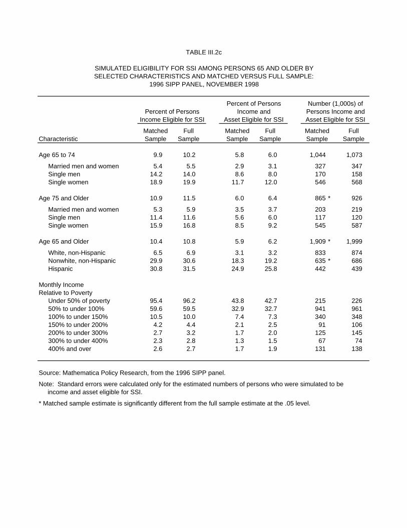
TABLE III.2c

SIMULATED ELIGIBILITY FOR SSI AMONG PERSONS 65 AND OLDER BYSELECTED CHARACTERISTICS AND MATCHED VERSUS FULL SAMPLE:

1996 SIPP PANEL, NOVEMBER 1998

Percent of Persons Number (1,000s) ofPercent of Persons Income and Persons Income and

Income Eligible for SSI Asset Eligible for SSI Asset Eligible for SSI

Matched Full Matched Full Matched FullCharacteristic Sample Sample Sample Sample Sample Sample

Age 65 to 74 9.9 10.2 5.8 6.0 1,044 1,073

Married men and women 5.4 5.5 2.9 3.1 327 347Single men 14.2 14.0 8.6 8.0 170 158Single women 18.9 19.9 11.7 12.0 546 568

Age 75 and Older 10.9 11.5 6.0 6.4 865 * 926

Married men and women 5.3 5.9 3.5 3.7 203 219Single men 11.4 11.6 5.6 6.0 117 120Single women 15.9 16.8 8.5 9.2 545 587

Age 65 and Older 10.4 10.8 5.9 6.2 1,909 * 1,999

White, non-Hispanic 6.5 6.9 3.1 3.2 833 874Nonwhite, non-Hispanic 29.9 30.6 18.3 19.2 635 * 686Hispanic 30.8 31.5 24.9 25.8 442 439

Monthly IncomeRelative to Poverty

Under 50% of poverty 95.4 96.2 43.8 42.7 215 22650% to under 100% 59.6 59.5 32.9 32.7 941 961100% to under 150% 10.5 10.0 7.4 7.3 340 348150% to under 200% 4.2 4.4 2.1 2.5 91 106200% to under 300% 2.7 3.2 1.7 2.0 125 145300% to under 400% 2.3 2.8 1.3 1.5 67 74400% and over 2.6 2.7 1.7 1.9 131 138

Source: Mathematica Policy Research, from the 1996 SIPP panel.

Note: Standard errors were calculated only for the estimated numbers of persons who were simulated to be income and asset eligible for SSI.

* Matched sample estimate is significantly different from the full sample estimate at the .05 level.

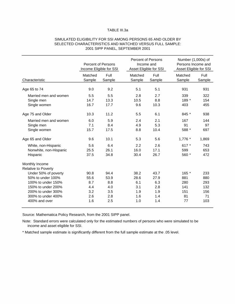
TABLE III.3a

SIMULATED ELIGIBILITY FOR SSI AMONG PERSONS 65 AND OLDER BYSELECTED CHARACTERISTICS AND MATCHED VERSUS FULL SAMPLE:

2001 SIPP PANEL, SEPTEMBER 2001

Percent of Persons Number (1,000s) ofPercent of Persons Income and Persons Income and

Income Eligible for SSI Asset Eligible for SSI Asset Eligible for SSI

Matched Full Matched Full Matched FullCharacteristic Sample Sample Sample Sample Sample Sample

Age 65 to 74 9.0 9.2 5.1 5.1 931 931

Married men and women 5.5 5.5 2.8 2.7 339 322Single men 14.7 13.3 10.5 8.8 189 * 154Single women 16.7 17.7 9.6 10.3 403 455

Age 75 and Older 10.3 11.2 5.5 6.1 845 * 938

Married men and women 6.0 5.9 2.4 2.1 167 144Single men 7.1 8.4 4.9 5.3 91 97Single women 15.7 17.5 8.8 10.4 588 * 697

Age 65 and Older 9.6 10.1 5.3 5.6 1,776 * 1,869

White, non-Hispanic 5.6 6.4 2.2 2.6 617 * 743Nonwhite, non-Hispanic 25.5 26.1 16.0 17.1 599 653Hispanic 37.5 34.8 30.4 26.7 560 * 472

Monthly IncomeRelative to Poverty

Under 50% of poverty 90.8 94.4 38.2 43.7 165 * 23350% to under 100% 55.6 53.9 28.6 27.9 881 880100% to under 150% 8.7 8.8 6.1 6.3 280 293150% to under 200% 4.4 4.0 3.1 2.8 141 132200% to under 300% 3.2 3.5 1.9 1.9 151 156300% to under 400% 2.6 2.8 1.6 1.4 81 71400% and over 1.6 2.5 1.0 1.4 77 103

Source: Mathematica Policy Research, from the 2001 SIPP panel.

Note: Standard errors were calculated only for the estimated numbers of persons who were simulated to be income and asset eligible for SSI.

* Matched sample estimate is significantly different from the full sample estimate at the .05 level.

TABLE III.3b

SIMULATED ELIGIBILITY FOR SSI AMONG PERSONS 65 AND OLDER BYSELECTED CHARACTERISTICS AND MATCHED VERSUS FULL SAMPLE:

2001 SIPP PANEL, SEPTEMBER 2002

Percent of Persons Number (1,000s) ofPercent of Persons Income and Persons Income and

Income Eligible for SSI Asset Eligible for SSI Asset Eligible for SSI

Matched Full Matched Full Matched FullCharacteristic Sample Sample Sample Sample Sample Sample

Age 65 to 74 8.0 8.7 4.9 5.4 876 * 966

Married men and women 4.8 5.2 2.7 3.1 332 379Single men 14.0 12.6 9.5 8.4 156 133Single women 15.2 16.9 9.4 10.5 388 * 454

Age 75 and Older 9.4 10.5 6.1 6.5 965 * 1,036

Married men and women 5.4 5.7 3.4 3.2 250 234Single men 9.6 11.2 6.8 8.0 125 148Single women 13.7 15.4 8.9 9.7 590 654

Age 65 and Older 8.6 9.5 5.4 5.9 1,841 * 2,002

White, non-Hispanic 4.6 5.7 2.4 3.0 678 * 829Nonwhite, non-Hispanic 23.4 25.6 15.4 17.1 583 658Hispanic 36.2 33.8 28.3 27.0 580 515

Monthly IncomeRelative to Poverty

Under 50% of poverty 93.5 95.4 62.4 54.3 216 24750% to under 100% 55.6 55.9 35.5 34.8 999 1,033100% to under 150% 9.0 8.6 5.2 5.8 245 275150% to under 200% 5.3 4.6 4.2 3.5 188 157200% to under 300% 2.3 2.7 1.1 1.6 85 * 127300% to under 400% 2.0 2.6 0.9 1.2 48 61400% and over 1.1 2.0 0.7 1.2 60 * 101

Source: Mathematica Policy Research, from the 2001 SIPP panel.

Note: Standard errors were calculated only for the estimated numbers of persons who were simulated to be income and asset eligible for SSI.

* Matched sample estimate is significantly different from the full sample estimate at the .05 level.

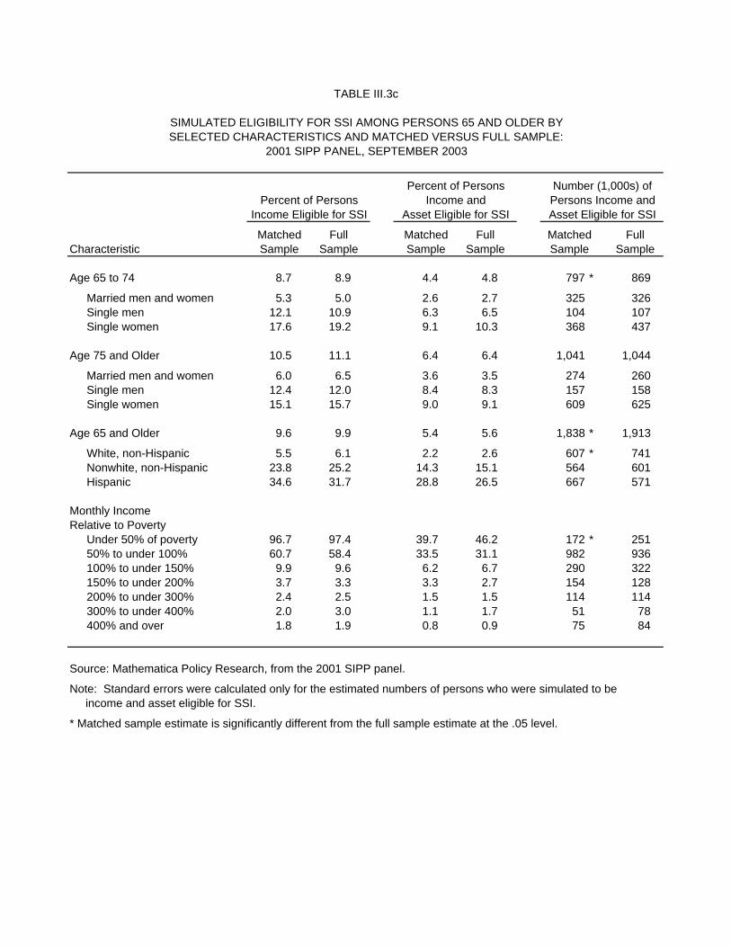
TABLE III.3c

SIMULATED ELIGIBILITY FOR SSI AMONG PERSONS 65 AND OLDER BYSELECTED CHARACTERISTICS AND MATCHED VERSUS FULL SAMPLE:

2001 SIPP PANEL, SEPTEMBER 2003

Percent of Persons Number (1,000s) ofPercent of Persons Income and Persons Income and

Income Eligible for SSI Asset Eligible for SSI Asset Eligible for SSI

Matched Full Matched Full Matched FullCharacteristic Sample Sample Sample Sample Sample Sample

Age 65 to 74 8.7 8.9 4.4 4.8 797 * 869

Married men and women 5.3 5.0 2.6 2.7 325 326Single men 12.1 10.9 6.3 6.5 104 107Single women 17.6 19.2 9.1 10.3 368 437

Age 75 and Older 10.5 11.1 6.4 6.4 1,041 1,044

Married men and women 6.0 6.5 3.6 3.5 274 260Single men 12.4 12.0 8.4 8.3 157 158Single women 15.1 15.7 9.0 9.1 609 625

Age 65 and Older 9.6 9.9 5.4 5.6 1,838 * 1,913

White, non-Hispanic 5.5 6.1 2.2 2.6 607 * 741Nonwhite, non-Hispanic 23.8 25.2 14.3 15.1 564 601Hispanic 34.6 31.7 28.8 26.5 667 571

Monthly IncomeRelative to Poverty

Under 50% of poverty 96.7 97.4 39.7 46.2 172 * 25150% to under 100% 60.7 58.4 33.5 31.1 982 936100% to under 150% 9.9 9.6 6.2 6.7 290 322150% to under 200% 3.7 3.3 3.3 2.7 154 128200% to under 300% 2.4 2.5 1.5 1.5 114 114300% to under 400% 2.0 3.0 1.1 1.7 51 78400% and over 1.8 1.9 0.8 0.9 75 84

Source: Mathematica Policy Research, from the 2001 SIPP panel.

Note: Standard errors were calculated only for the estimated numbers of persons who were simulated to be income and asset eligible for SSI.

* Matched sample estimate is significantly different from the full sample estimate at the .05 level.

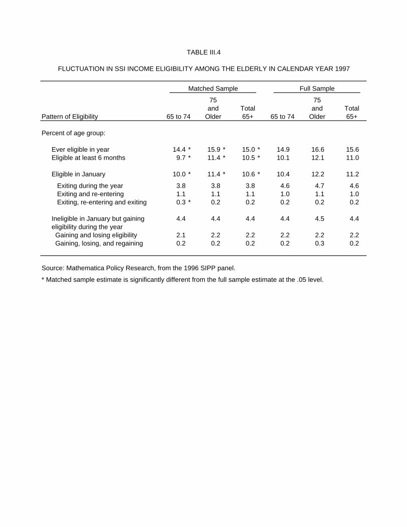
TABLE III.4

FLUCTUATION IN SSI INCOME ELIGIBILITY AMONG THE ELDERLY IN CALENDAR YEAR 1997

Matched Sample Full Sample

75 75and Total and Total

Pattern of Eligibility 65 to 74 Older 65+ 65 to 74 Older 65+

Percent of age group:

Ever eligible in year 14.4 * 15.9 * 15.0 * 14.9 16.6 15.6Eligible at least 6 months 9.7 * 11.4 * 10.5 * 10.1 12.1 11.0

Eligible in January 10.0 * 11.4 * 10.6 * 10.4 12.2 11.2

Exiting during the year 3.8 3.8 3.8 4.6 4.7 4.6 Exiting and re-entering 1.1 1.1 1.1 1.0 1.1 1.0 Exiting, re-entering and exiting 0.3 * 0.2 0.2 0.2 0.2 0.2

Ineligible in January but gaining 4.4 4.4 4.4 4.4 4.5 4.4eligibility during the year Gaining and losing eligibility 2.1 2.2 2.2 2.2 2.2 2.2 Gaining, losing, and regaining 0.2 0.2 0.2 0.2 0.3 0.2

Source: Mathematica Policy Research, from the 1996 SIPP panel.

* Matched sample estimate is significantly different from the full sample estimate at the .05 level.

TABLE III.5a

FLUCTUATION IN SSI INCOME ELIGIBILITY AMONG THE ELDERLY IN CALENDAR YEAR 2001

Matched Sample Full Sample

75 75and Total and Total

Pattern of Eligibility 65 to 74 Older 65+ 65 to 74 Older 65+

Percent of age group:

Ever eligible in year 14.5 * 16.4 15.3 * 15.8 17.2 16.4Eligible at least 6 months 8.3 * 8.7 8.5 * 9.1 9.6 9.3

Eligible in January 9.2 * 10.2 * 9.6 * 10.3 11.2 10.7

Exiting during the year 4.2 * 4.2 * 4.2 * 6.0 5.7 5.9 Exiting and re-entering 1.1 0.6 0.9 1.2 0.8 1.0 Exiting, re-entering and exiting 0.1 0.1 0.1 0.2 0.2 0.2

Ineligible in January but gaining 5.3 6.2 5.7 5.4 6.0 5.7eligibility during the year Gaining and losing eligibility 2.9 3.5 3.1 3.0 3.2 3.1 Gaining, losing, and regaining 0.2 0.2 0.2 0.2 0.2 0.2

Source: Mathematica Policy Research, from the 2001 SIPP panel.

* Matched sample estimate is significantly different from the full sample estimate at the .05 level.

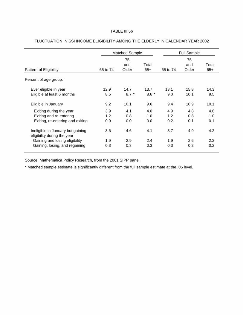
TABLE III.5b

FLUCTUATION IN SSI INCOME ELIGIBILITY AMONG THE ELDERLY IN CALENDAR YEAR 2002

Matched Sample Full Sample

75 75and Total and Total

Pattern of Eligibility 65 to 74 Older 65+ 65 to 74 Older 65+

Percent of age group:

Ever eligible in year 12.9 14.7 13.7 13.1 15.8 14.3Eligible at least 6 months 8.5 8.7 * 8.6 * 9.0 10.1 9.5

Eligible in January 9.2 10.1 9.6 9.4 10.9 10.1

Exiting during the year 3.9 4.1 4.0 4.9 4.8 4.8 Exiting and re-entering 1.2 0.8 1.0 1.2 0.8 1.0 Exiting, re-entering and exiting 0.0 0.0 0.0 0.2 0.1 0.1

Ineligible in January but gaining 3.6 4.6 4.1 3.7 4.9 4.2eligibility during the year Gaining and losing eligibility 1.9 2.9 2.4 1.9 2.6 2.2 Gaining, losing, and regaining 0.3 0.3 0.3 0.3 0.2 0.2

Source: Mathematica Policy Research, from the 2001 SIPP panel.

* Matched sample estimate is significantly different from the full sample estimate at the .05 level.

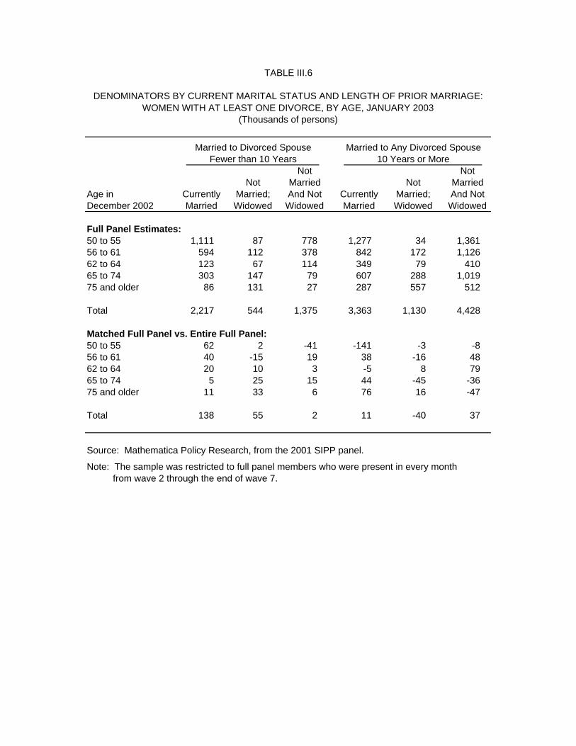
TABLE III.6

DENOMINATORS BY CURRENT MARITAL STATUS AND LENGTH OF PRIOR MARRIAGE:WOMEN WITH AT LEAST ONE DIVORCE, BY AGE, JANUARY 2003

(Thousands of persons)

Married to Divorced Spouse Married to Any Divorced SpouseFewer than 10 Years 10 Years or More

Not NotNot Married Not Married

Age in Currently Married; And Not Currently Married; And NotDecember 2002 Married Widowed Widowed Married Widowed Widowed

Full Panel Estimates:50 to 55 1,111 87 778 1,277 34 1,36156 to 61 594 112 378 842 172 1,12662 to 64 123 67 114 349 79 41065 to 74 303 147 79 607 288 1,01975 and older 86 131 27 287 557 512

Total 2,217 544 1,375 3,363 1,130 4,428

Matched Full Panel vs. Entire Full Panel:50 to 55 62 2 -41 -141 -3 -856 to 61 40 -15 19 38 -16 4862 to 64 20 10 3 -5 8 7965 to 74 5 25 15 44 -45 -3675 and older 11 33 6 76 16 -47

Total 138 55 2 11 -40 37

Source: Mathematica Policy Research, from the 2001 SIPP panel.

Note: The sample was restricted to full panel members who were present in every month from wave 2 through the end of wave 7.

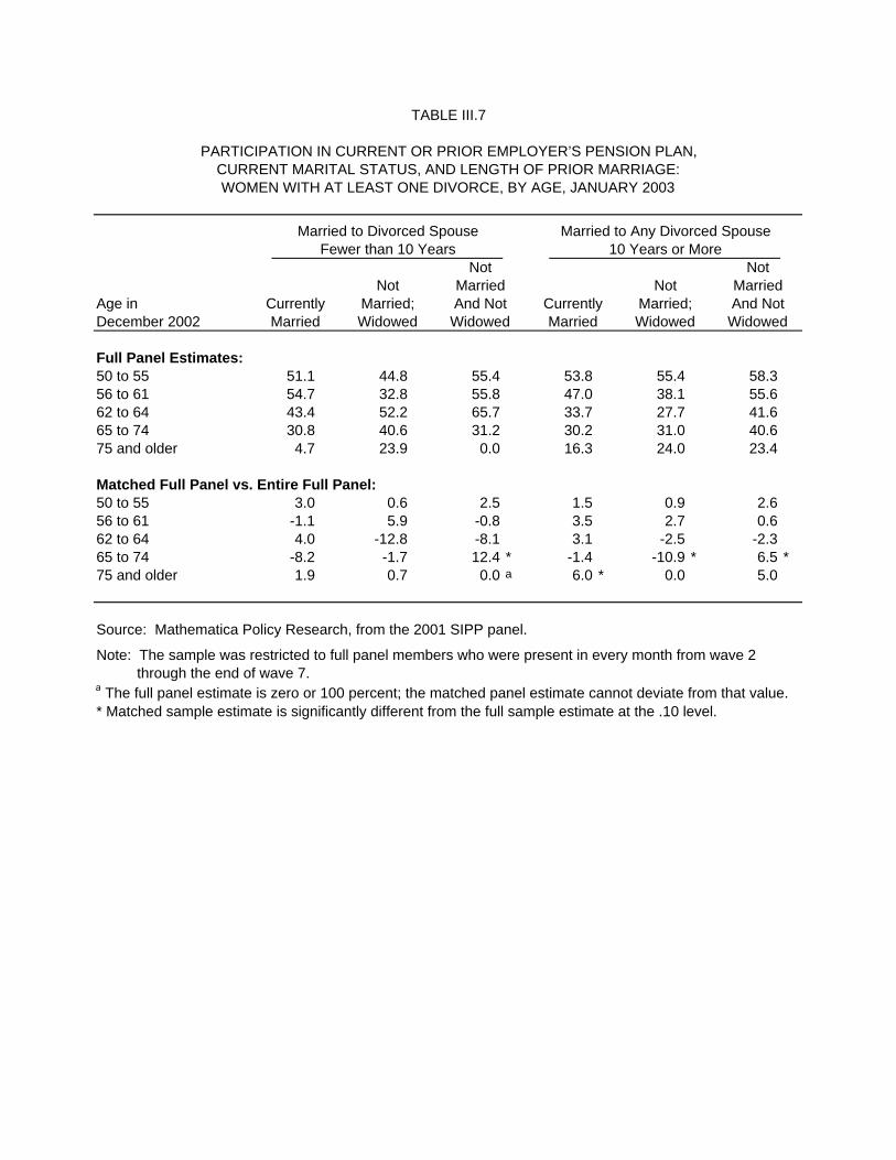
TABLE III.7

PARTICIPATION IN CURRENT OR PRIOR EMPLOYER’S PENSION PLAN,CURRENT MARITAL STATUS, AND LENGTH OF PRIOR MARRIAGE:WOMEN WITH AT LEAST ONE DIVORCE, BY AGE, JANUARY 2003

Married to Divorced Spouse Married to Any Divorced SpouseFewer than 10 Years 10 Years or More

Not NotNot Married Not Married

Age in Currently Married; And Not Currently Married; And NotDecember 2002 Married Widowed Widowed Married Widowed Widowed

Full Panel Estimates:50 to 55 51.1 44.8 55.4 53.8 55.4 58.356 to 61 54.7 32.8 55.8 47.0 38.1 55.662 to 64 43.4 52.2 65.7 33.7 27.7 41.665 to 74 30.8 40.6 31.2 30.2 31.0 40.675 and older 4.7 23.9 0.0 16.3 24.0 23.4

Matched Full Panel vs. Entire Full Panel:50 to 55 3.0 0.6 2.5 1.5 0.9 2.6 56 to 61 -1.1 5.9 -0.8 3.5 2.7 0.6 62 to 64 4.0 -12.8 -8.1 3.1 -2.5 -2.3 65 to 74 -8.2 -1.7 12.4 * -1.4 -10.9 * 6.5 *75 and older 1.9 0.7 0.0 a 6.0 * 0.0 5.0

Source: Mathematica Policy Research, from the 2001 SIPP panel.

Note: The sample was restricted to full panel members who were present in every month from wave 2 through the end of wave 7. a The full panel estimate is zero or 100 percent; the matched panel estimate cannot deviate from that value.* Matched sample estimate is significantly different from the full sample estimate at the .10 level.

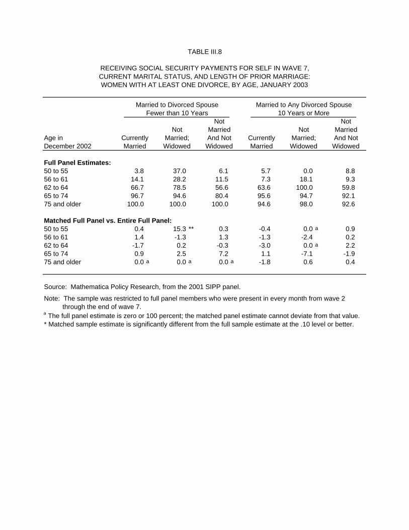
TABLE III.8

RECEIVING SOCIAL SECURITY PAYMENTS FOR SELF IN WAVE 7,CURRENT MARITAL STATUS, AND LENGTH OF PRIOR MARRIAGE:WOMEN WITH AT LEAST ONE DIVORCE, BY AGE, JANUARY 2003

Married to Divorced Spouse Married to Any Divorced SpouseFewer than 10 Years 10 Years or More

Not NotNot Married Not Married

Age in Currently Married; And Not Currently Married; And NotDecember 2002 Married Widowed Widowed Married Widowed Widowed

Full Panel Estimates:50 to 55 3.8 37.0 6.1 5.7 0.0 8.856 to 61 14.1 28.2 11.5 7.3 18.1 9.362 to 64 66.7 78.5 56.6 63.6 100.0 59.865 to 74 96.7 94.6 80.4 95.6 94.7 92.175 and older 100.0 100.0 100.0 94.6 98.0 92.6

Matched Full Panel vs. Entire Full Panel:50 to 55 0.4 15.3 ** 0.3 -0.4 0.0 a 0.9 56 to 61 1.4 -1.3 1.3 -1.3 -2.4 0.2 62 to 64 -1.7 0.2 -0.3 -3.0 0.0 a 2.2 65 to 74 0.9 2.5 7.2 1.1 -7.1 -1.9 75 and older 0.0 a 0.0 a 0.0 a -1.8 0.6 0.4

Source: Mathematica Policy Research, from the 2001 SIPP panel.

Note: The sample was restricted to full panel members who were present in every month from wave 2 through the end of wave 7. a The full panel estimate is zero or 100 percent; the matched panel estimate cannot deviate from that value.* Matched sample estimate is significantly different from the full sample estimate at the .10 level or better.

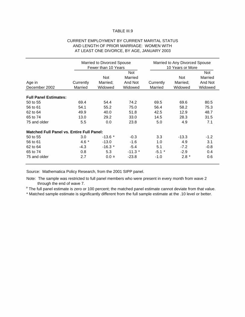
TABLE III.9

CURRENT EMPLOYMENT BY CURRENT MARITAL STATUSAND LENGTH OF PRIOR MARRIAGE: WOMEN WITHAT LEAST ONE DIVORCE, BY AGE, JANUARY 2003

Married to Divorced Spouse Married to Any Divorced SpouseFewer than 10 Years 10 Years or More

Not NotNot Married Not Married

Age in Currently Married; And Not Currently Married; And NotDecember 2002 Married Widowed Widowed Married Widowed Widowed

Full Panel Estimates:50 to 55 69.4 54.4 74.2 69.5 69.6 80.556 to 61 54.1 55.2 75.0 56.4 58.2 75.362 to 64 49.9 40.0 51.8 42.5 12.9 48.765 to 74 13.0 29.2 33.0 14.5 28.3 31.575 and older 5.5 0.0 23.8 5.0 4.9 7.1

Matched Full Panel vs. Entire Full Panel:50 to 55 3.0 -13.6 * -0.3 3.3 -13.3 -1.2 56 to 61 4.6 * -13.0 -1.6 1.0 4.9 3.1 62 to 64 -4.3 -16.3 * -5.4 5.1 -7.2 -0.8 65 to 74 0.8 5.3 -11.3 * -5.1 * -2.9 0.4 75 and older 2.7 0.0 a -23.8 -1.0 2.8 * 0.6

Source: Mathematica Policy Research, from the 2001 SIPP panel.

Note: The sample was restricted to full panel members who were present in every month from wave 2 through the end of wave 7. a The full panel estimate is zero or 100 percent; the matched panel estimate cannot deviate from that value.* Matched sample estimate is significantly different from the full sample estimate at the .10 level or better.

TABLE III.10

ANNUAL INCOME-TO-POVERTY RATIO IS UNDER 200 PERCENT IN 2002,CURRENT MARITAL STATUS, AND LENGTH OF PRIOR MARRIAGE:WOMEN WITH AT LEAST ONE DIVORCE, BY AGE, JANUARY 2003

Married to Divorced Spouse Married to Any Divorced SpouseFewer than 10 Years 10 Years or More

Not NotNot Married Not Married

Age in Currently Married; And Not Currently Married; And NotDecember 2002 Married Widowed Widowed Married Widowed Widowed

Full Panel Estimates:50 to 55 12.7 55.6 42.7 10.9 28.3 30.056 to 61 16.3 38.5 32.9 17.4 48.6 32.262 to 64 20.1 52.5 14.9 6.4 54.0 46.165 to 74 26.7 43.4 57.3 19.1 52.7 49.975 and older 35.9 57.5 76.2 23.6 60.1 56.4

Matched Full Panel vs. Entire Full Panel:50 to 55 -0.8 8.2 2.9 0.8 -10.4 -1.0 56 to 61 -0.2 -7.5 -1.5 -2.3 -2.0 -4.6 *62 to 64 4.9 14.0 * 7.1 -1.9 -3.3 -1.1 65 to 74 6.0 -1.3 -5.9 -0.9 -11.0 * -0.8 75 and older 7.8 0.4 23.8 1.1 -5.4 -3.5

Source: Mathematica Policy Research, from the 2001 SIPP panel.

Note: The sample was restricted to full panel members who were present in every month from wave 2 through the end of wave 7. a The full panel estimate is zero or 100 percent; the matched panel estimate cannot deviate from that value.* Matched sample estimate is significantly different from the full sample estimate at the .10 level or better.

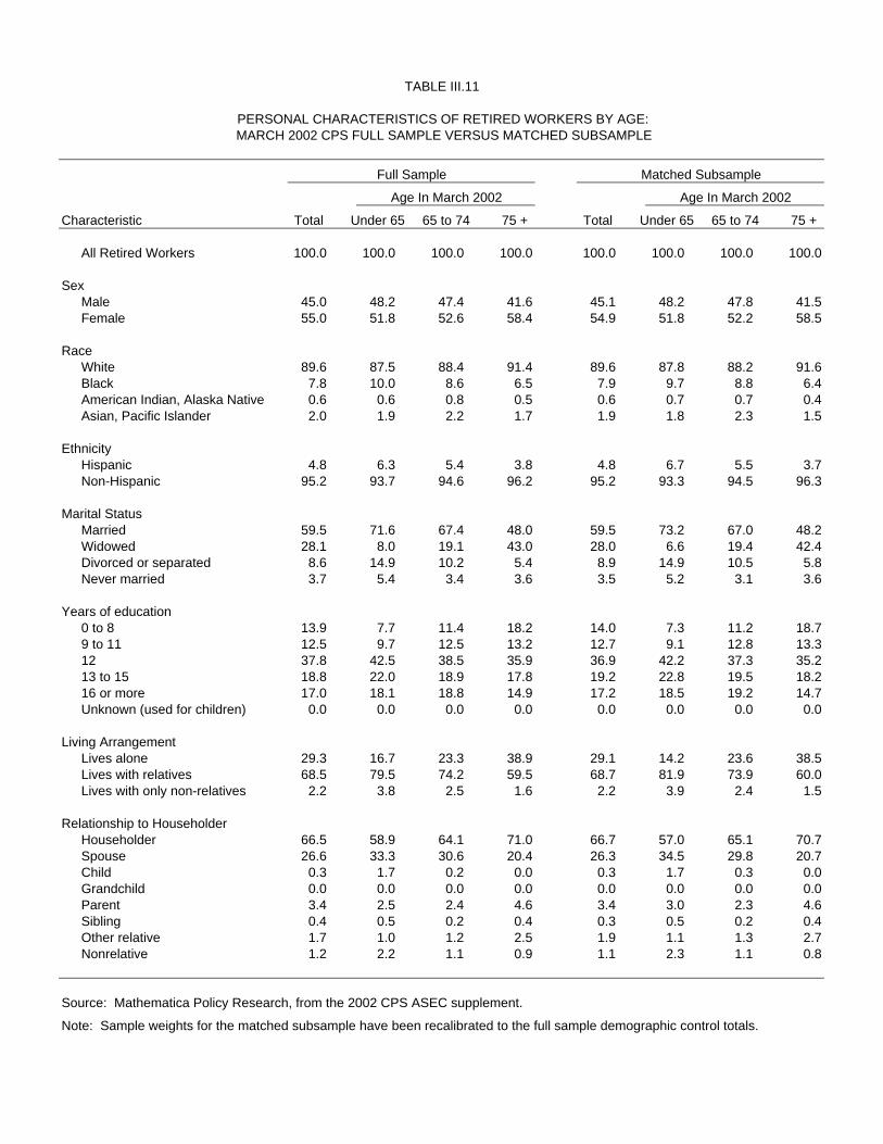
TABLE III.11

PERSONAL CHARACTERISTICS OF RETIRED WORKERS BY AGE:MARCH 2002 CPS FULL SAMPLE VERSUS MATCHED SUBSAMPLE

Full Sample Matched Subsample

Age In March 2002 Age In March 2002

Characteristic Total Under 65 65 to 74 75 + Total Under 65 65 to 74 75 +

All Retired Workers 100.0 100.0 100.0 100.0 100.0 100.0 100.0 100.0

SexMale 45.0 48.2 47.4 41.6 45.1 48.2 47.8 41.5Female 55.0 51.8 52.6 58.4 54.9 51.8 52.2 58.5

RaceWhite 89.6 87.5 88.4 91.4 89.6 87.8 88.2 91.6Black 7.8 10.0 8.6 6.5 7.9 9.7 8.8 6.4American Indian, Alaska Native 0.6 0.6 0.8 0.5 0.6 0.7 0.7 0.4Asian, Pacific Islander 2.0 1.9 2.2 1.7 1.9 1.8 2.3 1.5

EthnicityHispanic 4.8 6.3 5.4 3.8 4.8 6.7 5.5 3.7Non-Hispanic 95.2 93.7 94.6 96.2 95.2 93.3 94.5 96.3

Marital StatusMarried 59.5 71.6 67.4 48.0 59.5 73.2 67.0 48.2Widowed 28.1 8.0 19.1 43.0 28.0 6.6 19.4 42.4Divorced or separated 8.6 14.9 10.2 5.4 8.9 14.9 10.5 5.8Never married 3.7 5.4 3.4 3.6 3.5 5.2 3.1 3.6

Years of education0 to 8 13.9 7.7 11.4 18.2 14.0 7.3 11.2 18.79 to 11 12.5 9.7 12.5 13.2 12.7 9.1 12.8 13.312 37.8 42.5 38.5 35.9 36.9 42.2 37.3 35.213 to 15 18.8 22.0 18.9 17.8 19.2 22.8 19.5 18.216 or more 17.0 18.1 18.8 14.9 17.2 18.5 19.2 14.7Unknown (used for children) 0.0 0.0 0.0 0.0 0.0 0.0 0.0 0.0

Living ArrangementLives alone 29.3 16.7 23.3 38.9 29.1 14.2 23.6 38.5Lives with relatives 68.5 79.5 74.2 59.5 68.7 81.9 73.9 60.0Lives with only non-relatives 2.2 3.8 2.5 1.6 2.2 3.9 2.4 1.5

Relationship to HouseholderHouseholder 66.5 58.9 64.1 71.0 66.7 57.0 65.1 70.7Spouse 26.6 33.3 30.6 20.4 26.3 34.5 29.8 20.7Child 0.3 1.7 0.2 0.0 0.3 1.7 0.3 0.0Grandchild 0.0 0.0 0.0 0.0 0.0 0.0 0.0 0.0Parent 3.4 2.5 2.4 4.6 3.4 3.0 2.3 4.6Sibling 0.4 0.5 0.2 0.4 0.3 0.5 0.2 0.4Other relative 1.7 1.0 1.2 2.5 1.9 1.1 1.3 2.7Nonrelative 1.2 2.2 1.1 0.9 1.1 2.3 1.1 0.8

Source: Mathematica Policy Research, from the 2002 CPS ASEC supplement.

Note: Sample weights for the matched subsample have been recalibrated to the full sample demographic control totals.

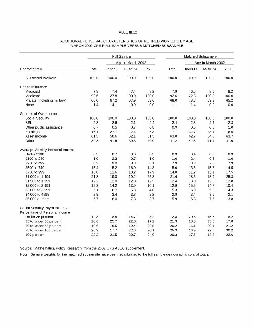
TABLE III.12

ADDITIONAL PERSONAL CHARACTERISTICS OF RETIRED WORKERS BY AGE:MARCH 2002 CPS FULL SAMPLE VERSUS MATCHED SUBSAMPLE

Full Sample Matched Subsample

Age In March 2002 Age In March 2002

Characteristic Total Under 65 65 to 74 75 + Total Under 65 65 to 74 75 +

All Retired Workers 100.0 100.0 100.0 100.0 100.0 100.0 100.0 100.0

Health InsuranceMedicaid 7.8 7.4 7.4 8.2 7.9 6.6 8.0 8.2Medicare 92.6 27.8 100.0 100.0 92.6 22.8 100.0 100.0Private (including military) 66.0 67.2 67.9 63.6 68.0 73.8 69.3 65.2None 1.4 14.1 0.0 0.0 1.1 11.4 0.0 0.0

Sources of Own IncomeSocial Security 100.0 100.0 100.0 100.0 100.0 100.0 100.0 100.0SSI 2.3 2.6 2.1 2.4 2.4 2.8 2.4 2.3Other public assistance 0.7 0.5 0.7 0.8 0.9 0.5 0.8 1.0Earnings 16.1 27.7 22.4 6.3 17.1 32.7 23.4 6.5Asset income 61.5 58.6 62.1 61.5 63.8 62.7 64.0 63.7Other 39.8 41.5 39.3 40.0 41.2 42.8 41.1 41.0

Average Monthly Personal IncomeUnder $100 0.3 0.7 0.3 0.3 0.3 0.4 0.2 0.3$100 to 249 1.0 2.3 0.7 1.0 1.0 2.4 0.6 1.0$250 to 499 8.3 9.0 8.3 8.1 7.9 8.3 7.8 7.9$500 to 749 15.4 15.2 16.0 14.8 15.0 13.6 15.7 14.5$750 to 999 15.0 11.6 13.2 17.9 14.8 11.2 13.1 17.5$1,000 to 1,499 21.8 19.0 19.2 25.3 21.6 18.5 18.9 25.3$1,500 to 1,999 12.2 12.0 12.0 12.5 12.4 13.0 12.0 12.8$2,000 to 2,999 12.3 14.2 13.9 10.1 12.9 15.5 14.7 10.4$3,000 to 3,999 5.1 6.7 5.8 4.0 5.3 6.9 5.9 4.3$4,000 to 4999 2.9 3.4 3.3 2.2 2.9 3.4 3.5 2.1$5,000 or more 5.7 6.0 7.3 3.7 5.9 6.8 7.6 3.8

Social Security Payments as aPercentage of Personal Income

Under 25 percent 12.3 18.5 14.7 8.2 12.8 20.6 15.5 8.225 to under 50 percent 20.6 25.7 22.6 17.2 21.3 28.8 23.0 17.850 to under 75 percent 19.6 16.5 19.4 20.5 20.2 16.1 20.1 21.275 to under 100 percent 25.3 17.7 22.6 30.1 25.3 16.9 22.6 30.2100 percent 22.2 21.5 20.7 24.0 20.3 17.5 18.8 22.6

Source: Mathematica Policy Research, from the 2002 CPS ASEC supplement.

Note: Sample weights for the matched subsample have been recalibrated to the full sample demographic control totals.

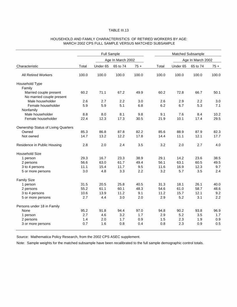
TABLE III.13

HOUSEHOLD AND FAMILY CHARACTERISTICS OF RETIRED WORKERS BY AGE:MARCH 2002 CPS FULL SAMPLE VERSUS MATCHED SUBSAMPLE

Full Sample Matched Subsample

Age In March 2002 Age In March 2002

Characteristic Total Under 65 65 to 74 75 + Total Under 65 65 to 74 75 +

All Retired Workers 100.0 100.0 100.0 100.0 100.0 100.0 100.0 100.0

Household TypeFamily Married couple present 60.2 71.1 67.2 49.9 60.2 72.8 66.7 50.1 No married couple present Male householder 2.6 2.7 2.2 3.0 2.6 2.9 2.2 3.0 Female householder 5.9 5.9 5.1 6.8 6.2 6.7 5.3 7.1Nonfamily Male householder 8.8 8.0 8.1 9.8 9.1 7.6 8.4 10.2 Female householder 22.4 12.3 17.3 30.5 21.9 10.1 17.4 29.5

Ownership Status of Living QuartersOwned 85.3 86.8 87.8 82.2 85.6 88.9 87.9 82.3Not owned 14.7 13.2 12.2 17.8 14.4 11.1 12.1 17.7

Residence in Public Housing 2.8 2.0 2.4 3.5 3.2 2.0 2.7 4.0

Household Size1 person 29.3 16.7 23.3 38.9 29.1 14.2 23.6 38.52 persons 56.6 63.0 61.7 49.4 56.1 63.1 60.5 49.53 to 4 persons 11.1 15.4 11.7 9.5 11.6 16.9 12.3 9.75 or more persons 3.0 4.8 3.3 2.2 3.2 5.7 3.5 2.4

Family Size1 person 31.5 20.5 25.8 40.5 31.3 18.1 26.1 40.02 persons 55.2 61.1 60.1 48.3 54.6 61.0 58.7 48.63 to 4 persons 10.6 13.9 11.2 9.1 11.2 15.7 12.1 9.25 or more persons 2.7 4.4 3.0 2.0 2.9 5.2 3.1 2.2

Persons under 18 in FamilyNone 95.2 91.8 94.4 97.0 94.8 90.2 93.8 96.91 person 2.7 4.6 3.2 1.7 2.9 5.2 3.5 1.72 persons 1.4 2.0 1.7 0.9 1.5 2.3 1.9 0.93 or more persons 0.7 1.6 0.8 0.4 0.8 2.3 0.9 0.5

Source: Mathematica Policy Research, from the 2002 CPS ASEC supplement.

Note: Sample weights for the matched subsample have been recalibrated to the full sample demographic control totals.

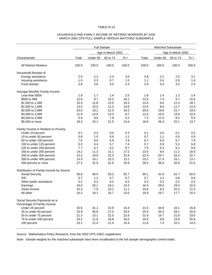
TABLE III.14

HOUSEHOLD AND FAMILY INCOME OF RETIRED WORKERS BY AGE:MARCH 2002 CPS FULL SAMPLE VERSUS MATCHED SUBSAMPLE

Full Sample Matched Subsample

Age In March 2002 Age In March 2002

Characteristic Total Under 65 65 to 74 75 + Total Under 65 65 to 74 75 +

All Retired Workers 100.0 100.0 100.0 100.0 100.0 100.0 100.0 100.0

Household Receipt of:Energy assistance 2.6 2.2 2.3 3.0 2.8 2.2 2.5 3.1Housing assistance 1.0 0.3 0.7 1.5 1.1 0.4 0.9 1.6Food stamps 2.8 3.8 3.0 2.4 2.9 3.3 3.3 2.4

Average Monthly Family IncomeLess than $500 1.9 1.7 1.4 2.5 1.8 1.4 1.3 2.4$500 to 999 12.6 9.7 10.2 16.1 12.0 7.4 9.7 15.5$1,000 to 1,499 15.3 11.8 12.5 19.3 14.4 9.6 11.4 18.7$1,500 to 1,999 13.0 10.0 12.3 14.5 12.5 8.6 11.7 14.3$2,000 to 2,999 20.0 19.1 21.0 19.2 20.6 19.6 21.7 19.5$3,000 to 3,999 11.9 14.8 13.3 9.7 12.6 15.5 13.9 10.4$4,000 to 4,999 6.9 9.9 7.8 5.2 7.3 11.5 8.2 5.5$5,000 or more 18.3 23.1 21.5 13.4 18.9 26.3 22.1 13.7

Family Income in Relation to PovertyUnder 10 percent 0.1 0.2 0.0 0.2 0.1 0.0 0.1 0.210 to under 50 percent 0.8 1.0 0.6 1.1 0.7 1.1 0.5 0.950 to under 100 percent 7.0 8.6 5.9 7.8 6.7 6.9 5.7 7.9100 to under 125 percent 6.3 4.4 5.7 7.4 5.7 3.6 5.1 6.8125 to under 150 percent 7.7 6.7 6.2 9.7 7.5 5.3 6.1 9.6150 to under 200 percent 14.2 11.3 12.1 17.2 13.5 9.6 11.2 16.9200 to under 300 percent 22.2 19.9 22.3 22.6 22.4 20.7 22.4 22.7300 to under 400 percent 14.4 16.1 15.2 13.1 15.2 17.4 16.1 13.7400 percent or more 27.2 31.9 31.9 20.9 28.2 35.4 32.9 21.5

Distribution of Family Income by SourceSocial Security 56.6 46.5 53.2 62.7 55.1 41.6 51.7 62.0SSI 0.7 1.1 0.7 0.7 0.7 1.2 0.8 0.6Other public assistance 0.2 0.2 0.2 0.2 0.2 0.2 0.2 0.2Earnings 16.0 25.1 19.1 10.3 16.4 29.0 19.3 10.3Asset income 10.3 7.9 10.1 11.1 10.6 8.4 10.3 11.5All other 16.2 19.1 16.7 15.0 16.9 19.7 17.7 15.3

Social Security Payments as aPercentage of Family Income

Under 25 percent 20.6 31.1 22.9 15.4 21.5 34.8 24.1 15.825 to under 50 percent 24.9 30.8 27.5 20.5 25.5 33.3 28.1 20.950 to under 75 percent 21.3 15.1 21.5 22.6 21.9 14.7 21.8 23.575 to under 100 percent 20.2 11.6 16.8 26.0 19.5 9.8 15.9 25.6100 percent 13.1 11.4 11.4 15.4 11.6 7.3 10.1 14.3

Source: Mathematica Policy Research, from the 2002 CPS ASEC supplement.

Note: Sample weights for the matched subsample have been recalibrated to the full sample demographic control totals.

TABLE III.15

PERSONAL CHARACTERISTICS OF RETIRED WORKERS BY AGE, MARCH 2002 CPS:ALL SUPPLEMENT RESPONDENTS VERSUS MATCHED SUBSAMPLE

All Respondents to Supplement Matched Subsample of Respondents

Age In March 2002 Age In March 2002

Characteristic Total Under 65 65 to 74 75 + Total Under 65 65 to 74 75 +

All Retired Workers 100.0 100.0 100.0 100.0 100.0 100.0 100.0 100.0

SexMale 45.1 48.1 47.6 41.7 45.1 48.2 47.8 41.5Female 54.9 51.9 52.4 58.3 54.9 51.8 52.2 58.5

RaceWhite 89.8 87.7 88.6 91.5 89.8 88.3 88.4 91.7Black 7.8 10.1 8.5 6.5 7.8 9.4 8.7 6.4American Indian, Alaska Native 0.6 0.6 0.8 0.5 0.6 0.6 0.8 0.4Asian, Pacific Islander 1.7 1.6 2.1 1.5 1.8 1.7 2.2 1.5

EthnicityHispanic 4.8 6.2 5.4 3.8 4.8 6.5 5.4 3.8Non-Hispanic 95.2 93.8 94.6 96.2 95.2 93.5 94.6 96.2

Marital StatusMarried 59.4 71.4 66.9 48.2 59.3 72.6 66.7 48.2Widowed 28.2 8.1 19.3 42.8 28.1 6.8 19.5 42.3Divorced or separated 8.8 15.3 10.4 5.4 9.1 15.4 10.7 5.9Never married 3.7 5.3 3.4 3.6 3.5 5.2 3.1 3.6

Years of education0 to 8 13.9 7.7 11.3 18.3 14.0 7.5 11.1 18.69 to 11 12.5 9.5 12.5 13.1 12.6 9.0 12.8 13.312 37.7 42.2 38.3 36.0 37.1 42.1 37.7 35.413 to 15 18.8 21.7 19.2 17.7 19.1 22.3 19.4 18.016 or more 17.1 18.9 18.7 14.9 17.2 19.1 19.1 14.7Unknown (used for children) 0.0 0.0 0.0 0.0 0.0 0.0 0.0 0.0

Living ArrangementLives alone 29.4 16.7 23.6 38.7 29.3 14.7 23.8 38.6Lives with relatives 68.4 79.7 73.8 59.8 68.5 81.6 73.7 59.9Lives with only non-relatives 2.2 3.6 2.5 1.6 2.2 3.7 2.5 1.4

Relationship to HouseholderHouseholder 66.8 58.6 64.8 71.0 67.0 57.0 65.4 70.9Spouse 26.4 33.6 30.2 20.5 26.2 34.4 29.7 20.6Child 0.3 1.7 0.3 0.0 0.3 1.6 0.2 0.0Grandchild 0.0 0.0 0.0 0.0 0.0 0.0 0.0 0.0Parent 3.3 2.5 2.3 4.6 3.3 3.1 2.2 4.5Sibling 0.3 0.5 0.2 0.4 0.3 0.5 0.2 0.4Other relative 1.7 1.1 1.0 2.6 1.9 1.2 1.2 2.7Nonrelative 1.1 2.0 1.2 0.9 1.1 2.2 1.1 0.8

Source: Mathematica Policy Research, from the 2002 CPS ASEC supplement.

Note: Sample weights for all supplement respondents and the matched subsample have been recalibrated to the full sample demographic control totals.

TABLE III.16

ADDITIONAL PERSONAL CHARACTERISTICS OF RETIRED WORKERS BY AGE, MARCH 2002 CPS:ALL SUPPLEMENT RESPONDENTS VERSUS MATCHED SUBSAMPLE

Full Sample Matched Subsample

Age In March 2002 Age In March 2002

Characteristic Total Under 65 65 to 74 75 + Total Under 65 65 to 74 75 +

All Retired Workers 100.0 100.0 100.0 100.0 100.0 100.0 100.0 100.0

Health InsuranceMedicaid 7.7 6.8 7.6 8.0 7.9 6.4 7.9 8.2Medicare 92.7 26.5 100.0 100.0 92.6 21.8 100.0 100.0Private (including military) 66.8 71.2 68.3 64.1 68.4 75.5 69.6 65.5None 1.1 11.4 0.0 0.0 1.0 10.4 0.0 0.0

Sources of Own IncomeSocial Security 100.0 100.0 100.0 100.0 100.0 100.0 100.0 100.0SSI 2.2 2.6 2.1 2.3 2.4 2.7 2.3 2.3Other public assistance 0.8 0.5 0.7 0.9 0.9 0.6 0.9 1.0Earnings 16.2 29.7 22.5 6.1 17.2 34.0 23.7 6.4Asset income 61.6 59.5 62.1 61.6 63.8 63.5 64.0 63.7Other 40.0 41.8 39.3 40.3 41.5 43.6 41.2 41.4

Average Monthly Personal IncomeUnder $100 0.3 0.6 0.3 0.3 0.3 0.2 0.2 0.3$100 to 249 1.0 2.5 0.7 0.9 0.9 2.5 0.6 1.0$250 to 499 8.2 8.7 8.1 8.1 7.7 7.8 7.6 7.9$500 to 749 15.3 14.7 15.9 14.7 15.1 13.5 15.8 14.5$750 to 999 15.1 11.2 13.3 18.0 14.8 10.9 13.1 17.6$1,000 to 1,499 21.8 18.8 19.2 25.4 21.8 18.6 19.1 25.5$1,500 to 1,999 12.2 12.0 12.0 12.5 12.4 13.2 12.0 12.6$2,000 to 2,999 12.3 14.8 14.0 9.9 12.9 16.0 14.8 10.2$3,000 to 3,999 5.1 6.8 5.7 4.1 5.3 7.2 5.8 4.4$4,000 to 4999 2.8 3.4 3.4 2.1 2.9 3.4 3.4 2.1$5,000 or more 5.7 6.4 7.4 3.8 5.9 6.7 7.5 3.9

Social Security Payments as aPercentage of Personal Income

Under 25 percent 12.4 19.5 14.7 8.1 12.9 21.0 15.3 8.425 to under 50 percent 20.7 26.7 22.6 17.1 21.5 29.9 23.1 17.750 to under 75 percent 19.6 17.0 19.4 20.5 20.1 16.5 20.1 20.975 to under 100 percent 25.2 16.6 22.5 30.2 25.3 16.2 22.6 30.3100 percent 22.2 20.3 20.8 24.1 20.3 16.4 18.9 22.6

Source: Mathematica Policy Research, from the 2002 CPS ASEC supplement.

Note: Sample weights for all supplement respondents and the matched subsample have been recalibrated to the full sample demographic control totals.

TABLE III.17

HOUSEHOLD AND FAMILY CHARACTERISTICS OF RETIRED WORKERS BY AGE, MARCH 2002 CPS:ALL SUPPLEMENT RESPONDENTS VERSUS MATCHED SUBSAMPLE

Full Sample Matched Subsample

Age In March 2002 Age In March 2002

Characteristic Total Under 65 65 to 74 75 + Total Under 65 65 to 74 75 +

All Retired Workers 100.0 100.0 100.0 100.0 100.0 100.0 100.0 100.0

Household TypeFamily Married couple present 60.0 70.7 66.6 50.2 59.9 72.4 66.3 50.1 No married couple present Male householder 2.7 3.0 2.3 3.0 2.6 2.9 2.2 2.9 Female householder 6.0 6.3 5.2 6.8 6.3 6.6 5.4 7.2Nonfamily Male householder 8.8 8.0 8.2 9.7 9.2 7.5 8.5 10.3 Female householder 22.5 12.1 17.6 30.3 22.0 10.6 17.5 29.5

Ownership Status of Living QuartersOwned 85.5 87.3 87.8 82.4 85.6 89.0 87.9 82.4Not owned 14.5 12.7 12.2 17.6 14.4 11.0 12.1 17.6

Residence in Public Housing 3.0 2.3 2.5 3.6 3.3 2.1 2.8 4.1

Household Size1 person 29.4 16.7 23.6 38.7 29.3 14.7 23.8 38.62 persons 56.8 63.5 61.8 49.8 56.2 63.5 60.6 49.63 to 4 persons 11.0 15.2 11.4 9.5 11.5 16.5 12.2 9.65 or more persons 2.8 4.5 3.2 2.0 3.0 5.3 3.4 2.2

Family Size1 person 31.6 20.3 26.2 40.2 31.5 18.4 26.3 40.12 persons 55.4 61.6 60.1 48.7 54.7 61.3 58.8 48.73 to 4 persons 10.5 14.0 10.9 9.1 11.1 15.4 11.9 9.25 or more persons 2.6 4.2 2.9 1.9 2.8 4.9 3.0 2.0

Persons under 18 in FamilyNone 95.3 91.8 94.5 97.1 94.9 90.6 93.9 97.01 person 2.6 4.7 3.1 1.7 2.8 5.0 3.4 1.82 persons 1.3 2.0 1.6 0.9 1.4 2.2 1.8 0.83 or more persons 0.7 1.6 0.8 0.4 0.8 2.2 0.9 0.4

Source: Mathematica Policy Research, from the 2002 CPS ASEC supplement.

Note: Sample weights for all supplement respondents and the matched subsample have been recalibrated to the full sample demographic control totals.

TABLE III.18

HOUSEHOLD AND FAMILY INCOME OF RETIRED WORKERS BY AGE, MARCH 2002 CPS:ALL SUPPLEMENT RESPONDENTS VERSUS MATCHED SUBSAMPLE

Full Sample Matched Subsample

Age In March 2002 Age In March 2002

Characteristic Total Under 65 65 to 74 75 + Total Under 65 65 to 74 75 +

All Retired Workers 100.0 100.0 100.0 100.0 100.0 100.0 100.0 100.0

Household Receipt of:Energy assistance 2.6 2.4 2.4 2.9 2.9 2.3 2.6 3.2Housing assistance 1.0 0.3 0.7 1.4 1.1 0.4 0.9 1.6Food stamps 2.8 3.5 3.2 2.1 2.9 3.3 3.3 2.3

Average Monthly Family IncomeLess than $500 1.9 1.8 1.5 2.4 1.7 1.3 1.2 2.3$500 to 999 12.6 9.1 10.3 16.0 12.1 7.6 9.8 15.6$1,000 to 1,499 15.3 11.4 12.5 19.3 14.4 9.2 11.4 18.9$1,500 to 1,999 13.0 10.0 12.1 14.7 12.6 8.8 11.8 14.4$2,000 to 2,999 20.2 18.9 21.3 19.4 20.6 19.5 21.8 19.5$3,000 to 3,999 12.0 14.8 13.3 9.8 12.6 15.8 14.0 10.3$4,000 to 4,999 6.9 10.7 7.7 5.2 7.4 12.0 8.3 5.3$5,000 or more 18.0 23.4 21.3 13.2 18.5 25.8 21.6 13.5

Family Income in Relation to PovertyUnder 10 percent 0.1 0.2 0.0 0.2 0.1 0.0 0.1 0.210 to under 50 percent 0.8 0.9 0.6 1.0 0.7 0.9 0.5 0.850 to under 100 percent 6.9 8.4 6.0 7.7 6.8 7.3 5.7 7.9100 to under 125 percent 6.4 4.0 5.9 7.4 5.8 3.5 5.4 6.8125 to under 150 percent 7.7 6.3 6.2 9.8 7.5 5.0 5.9 9.8150 to under 200 percent 14.2 11.3 12.0 17.3 13.5 9.4 11.1 17.1200 to under 300 percent 22.2 19.4 22.4 22.7 22.4 20.3 22.5 22.7300 to under 400 percent 14.4 16.2 15.2 13.0 15.2 18.1 16.1 13.5400 percent or more 27.2 33.2 31.7 20.9 28.1 35.6 32.8 21.4

Distribution of Family Income by SourceSocial Security 56.6 45.4 53.4 62.8 55.2 41.4 51.9 62.0SSI 0.7 1.1 0.7 0.7 0.7 1.2 0.7 0.6Other public assistance 0.2 0.3 0.2 0.2 0.2 0.2 0.2 0.2Earnings 15.8 25.6 19.0 10.1 16.3 28.7 19.4 10.2Asset income 10.2 8.0 10.0 11.0 10.5 8.3 10.2 11.4All other 16.3 19.6 16.7 15.2 17.0 20.2 17.7 15.5

Social Security Payments as aPercentage of Family Income

Under 25 percent 20.4 31.8 22.7 15.2 21.4 34.6 23.9 15.825 to under 50 percent 24.9 31.2 27.3 20.7 25.6 33.7 28.2 20.950 to under 75 percent 21.5 15.9 21.7 22.6 21.9 15.3 21.9 23.275 to under 100 percent 20.0 10.2 16.7 26.0 19.5 9.1 15.9 25.7100 percent 13.2 10.9 11.7 15.5 11.7 7.3 10.1 14.4

Source: Mathematica Policy Research, from the 2002 CPS ASEC supplement.

Note: Sample weights for all supplement respondents and the matched subsample have been recalibrated to the full sample demographic control totals.

85

IV. ATTRITION BIAS IN THE SIPP

With each successive interview, fewer members of an initial SIPP panel respond. Excluding

those who have left the SIPP universe, this attrition of panel members may make the sample less

representative of the survivors of the population from which the initial sample was selected.

There is ample evidence from numerous studies over the years that people who attrite from panel

surveys—including the SIPP—are different from people who continue to respond.1 However,

SIPP sample weights—both cross-sectional and longitudinal—incorporate rather substantial

adjustments designed to reduce the bias that may result from attrition. This chapter looks at the

effectiveness of the adjustments that are included in the Census Bureau’s weights in

compensating for attrition bias and considers whether any refinement of these adjustments could

be beneficial to applications of SIPP panel data by SSA. We discuss methodological issues in

evaluating attrition bias in Section A and lay out our approach. In Section B we compare the full

panel sample and the wave 1 cross-sectional sample with respect to characteristics reported in the

SIPP. In Section C we extend the comparison to matched IRS and SSA administrative records.

Section D summarizes our major conclusions.

A. EVALUATING ATTRITION BIAS

Efforts to evaluate the bias associated with sample loss due to attrition confront three

notable limitations. First, survey data on attriters are available only prior to attrition. Second,

the survey data provided by eventual attriters could be of different quality than the data provided

by those who do not attrite. Third, while administrative records linked to survey records address

both of these limitations, administrative data are available only for matched observations, and the

1 See, for example, the collection of papers in The Journal of Human Resources, Vol. 33, No. 2, Special Issue:

Attrition in Longitudinal Surveys (Spring 1998).

86

decline in match rates is the single largest source of increased sample loss in the SIPP over the

period covered by this study.

Studies of attrition bias in panel surveys are typically limited to the panel survey data alone,

meaning that the attriters and non-attriters can be compared only with respect to characteristics

before attrition. Indeed, the two are often compared with respect to characteristics measured at

the initial interview because at that point, no one has attrited. For unchanging characteristics,

such as date of birth, sex, race, and ethnicity, such comparisons are informative about the impact

of attrition over the life of the panel. For characteristics that can change over time (and, in so

doing, provide the rationale for conducting longitudinal surveys in the first place), differences

between attriters and non-attriters at the initial interview may tell us little about the differences

that exist after attriters leave the sample, which is what we really want to know. More

sophisticated analyses, but still restricted to the panel data, can examine characteristics of

attriters not just at the initial interview but closer to the point of attrition—comparing the attriters

to non-attriters at the same point in time. Part of the intent of such analyses is to find evidence of

triggering events, such as a divorce, loss of employment, or birth of a child or death of a family

member. If there are triggering events, however, and especially if they are powerful, these

events may be more likely to occur after rather than prior to the last completed interview; if so,

they will not be captured in the survey data.

Another approach to evaluating attrition bias is to use aggregate data from an independent,

external source—such as a cross-sectional survey or a census—in order to determine how

attrition may have affected the distribution of characteristics in the panel survey. Comparability

of the measured variables across the surveys is a serious issue, of course. The most common

way to address this concern is to focus on trends rather than point-in-time measures, in which

case it is not as critical that the variables compared across surveys be identical as opposed to

87

merely similar. A comparison of poverty trends between the SIPP and the CPS, for example,

suggests that lower-income families are more likely than higher-income families to attrite. When

comparing estimates from panel surveys and cross-sectional surveys, however, one must also

account for factors besides attrition that contribute to the diminishing representativeness of most

panel surveys over time. Most importantly, additions to the population through immigration,

people returning from abroad, and people leaving institutions and the military are either not

represented, or they are under-represented in most panel surveys. The absence or

underrepresentation of these additions may induce a trend in the panel data that is not reflected in

a series of repeated cross-sections, which maintain consistent representativeness over time.

Even if the comparisons across surveys are effective and accurate, they are limited. They

may tell us about the impact of attrition on estimates of change at the aggregate level, or net

change, to borrow terminology from Vaughan and Scheuren (2002), but they tell us little about

the impact of attrition on estimates of gross change—that is, the changes experienced by

individuals.

Linked administrative and survey records make it possible to evaluate attrition bias directly.

If longitudinal administrative records can be linked to all persons present at the start of a panel

survey, then attriters and non-attriters can be compared with respect to characteristics measured

after as well as before attrition. Furthermore, attriters and non-attriters can be compared with

respect to their distributions of gross change rather than just their overall, net change.

Recent research by Vaughan and Scheuren (2002) and by Huynh et al. (2001) using SSA

administrative records matched to SIPP panel data produced similar findings with respect to both

earnings and program benefits.2 Attriters and non-attriters differ markedly with respect to their

2 Vaughan and Scheuren examined attrition in the SPD, which was selected from the 1992 and 1993 SIPP

panels.

88

characteristics at the beginning of the panel—that is, before attrition. Over time, however, these

differences attenuate. With enough passing years, the characteristics of those who attrited and

those who continued to respond to the survey converge. This trend suggests that compensating

for the impact of attrition on cross-sectional estimates becomes both easier and less important

over time. But the fact that the differences are large to begin with and then diminish over time

also implies that attriters experience greater change than non-attriters. Vaughan and Scheuren

suggest that compensating for the attrition bias in estimates of gross change is both important

and much more difficult than compensating for differences in net change.

SSA uses SIPP data in two main ways: (1) to support microsimulation modeling of

retirement behavior as well as eligibility for SSI and the Medicare Low Income Supplement and

(2) to provide detailed information on the characteristics of its beneficiary populations. For the

first application, SSA has tended to rely on the “full panel sample,” consisting of the subset of

respondents with data for as long as they remained in the SIPP universe. Members of the full

panel sample are assigned full panel weights, which incorporate a person-level non-interview

adjustment and calibration to wave 1 population controls. For the second application, SSA often

uses calendar year snapshots but has also used as little as a single wave. Clearly, attrition and the

possibility of attrition bias are concerns for both applications. Because the second application

may draw data from two or more time periods over the life of a SIPP panel, the potential impact

of attrition bias varies. Estimates of characteristics based on data drawn from the first year of a

SIPP panel will be less affected by attrition than estimates based on data from, say, the third year

of a panel. For the modeling applications using the full panel sample, respondents who attrited at

any point over the life of the panel are excluded, so the magnitude of attrition reflected in full

panel estimates is uniform over the entire length of the survey (although the impact on estimates

over the length of the panel may not be uniform).

89

In our evaluation of attrition bias in the SIPP, we focus on comparisons between the full

panel sample and the initial or wave 1 cross-sectional sample. Using the full panel sample

ensures that we will observe the maximum impact of attrition.3 At the same time, because full

panel weights are assigned to sample members who leave the survey universe (providing that

they have no missing data prior to their departure), using the full panel sample will ensure that

we do not confound universe leavers with attriters. As we explained in Chapter 2, people who

leave the survey universe differ in a number of ways from those who remain, but they are not

attriters and their exits from the survey universe are not counted as sample loss. By retaining

universe leavers in the full panel sample, we make certain that the differences between universe

leavers and those who remain in the population do not get folded into our estimates of attrition

bias.

Comparisons of the full panel sample and the wave 1 sample with respect to characteristics

measured in wave 1 of the SIPP can use the full wave 1 sample. Comparisons using

administrative records must exclude those full panel and wave 1 sample members who could not

be matched to administrative records. For the wave 1 sample, this includes sample members

who did not respond to the second wave of the survey, where SSNs were first requested. While

some of the wave 1 respondents who missed wave 2 responded to a later wave and were asked

for and provided their SSNs, we restricted the comparison sample to those wave 1 respondents

3 We note, however, that attriters are not the only sample members who are included in the wave 1 sample but

not the full panel sample. Respondents who missed a single wave—or even a single month within a single wave—would have been excluded from the 2001 full panel sample by the Census Bureau. By imputing missing waves, as the Census Bureau did prior to the 1996 panel, we could add such persons to the full panel sample, but this would require constructing an entirely new set of full panel weights to accommodate the expanded panel sample. In our evaluation of attrition bias we felt that it was important to be able to document the effectiveness of the Census Bureau’s panel weights before considering any additional adjustments.

90

who responded to the second wave (and could be matched to administrative records).4 For the

full panel sample it was not necessary to impose any additional restriction, as everyone who

qualified for a full panel weight responded to all nine waves and would have been asked to

provide an SSN (unless they left the survey universe immediately after the first wave).5

B. ASSESSMENT BASED ON SIPP CHARACTERISTICS

We estimated the magnitude of attrition bias in the estimates obtained from the full panel

sample by comparing weighted distributions of a wide range of demographic and economic

characteristics in wave 1 of the 2001 panel for all wave 1 respondents and those who qualified to

receive full panel weights. The sample estimates for all wave 1 respondents were weighted by

the January 2001 cross-sectional weight. The full panel sample estimates were weighted by the

Census Bureau’s full panel weight (LGTPNLWT). The full panel sample includes 64.4 percent

of the cross-sectional sample (or 64.6 percent if weighted by the cross-sectional weight; see table

II.2).6

Because of their large number, the 20 tables that present these comparisons are presented in

Appendix F. Estimates of bias with respect to personal demographic characteristics are reported

in Tables F.1.a through F.1.e, where the lower-case letters a through e refer to the total

population and four subpopulations of SSA beneficiaries: (b) retired workers, (c) disabled

4 We did so in order that we might be able to compare matched sample members and all sample members

among those who responded to both waves 1 and 2, as some of our comparisons required data collected in wave 2. See Chapter 3.

5 When we compare the matched full panel to the entire full panel sample, members of the latter who left the SIPP universe between the wave 1 and wave 2 interviews will not be represented in the matched data. This group is very small, however, accounting for only one-third of one percent of the sample, so the impact of its exclusion from the matched panel sample is negligible.

6 For the four subpopulations the full panel estimates include somewhat larger proportions of the corresponding wave 1 cross-sectional sample observations. These proportions, calculated from Table II.3 (and weighted by the January 2001 cross-sectional weight) are: 75.6 percent for retired workers, 72.1 percent for disabled workers, 72.7 percent for all other social security beneficiaries, and 66.3 percent for SSI recipients.

91

workers, (d) all other social security beneficiaries, and (e) SSI beneficiaries. In each table the

population or subpopulation is divided into three age groups, which vary by subpopulation.

Tables F.2.a through F.2.e provide estimates of attrition bias for an additional set of personal

characteristics, including personal income. Tables F.3.a through F.3.e provide estimates for

family and household demographic characteristics while Tables F.4.a through F.4.e report

estimates for several measures of family and household income. In each table the leftmost

columns report estimates for the cross-sectional sample while the rightmost columns report the

difference between the full panel and cross-sectional estimates with indicators of statistical

significance.

The overwhelming impression created by these comparisons is that the estimates for the full

panel sample and the wave 1 cross-sectional sample represent the same population. While we do

find some differences that are statistically significant and appear to be systematic, they are small.

The similarities in the two sets of estimates are far more striking. This is particularly true for the

several measures of income. This includes the distribution of average monthly total personal

income, the sources of own income, and the amount of social security benefits as a percentage of

total personal income in Tables F.2.a through F.2.e and all of the household and family income

measures in Tables F.4.a through F.4.e. For example, the amount of social security payments as

a percentage of total personal income is classified into five ranges. For the total population the

largest difference between the full panel and the cross-section is 0.1 percentage point (Table

F.2.a). For retired workers the differences range from zero to 0.3 percentage points—none

statistically significant (Table F.2.b). The range grows larger for disabled workers and other

social security beneficiaries but then smaller for SSI recipients, and none of the differences is

statistically significant. For total personal income for the total population, one category (under

$100) has a difference of 0.4 percentage points. For the remaining 10 categories the differences

92

are zero or 0.1 percentage point. For total household income for the total population the largest

difference is 0.3 percentage points while all of the rest are zero or 0.1 percentage point (Table

F.4.a). The proportion of households receiving food stamps differs by just 0.2 percentage points

for the total population, 0.3 percentage points for retired workers, zero for disabled workers, 0.1

percentage point for all other social security beneficiaries, and 1.8 percentage points for SSI

recipients (who have the largest food stamp participation rate by far).

The biggest differences are found in the family composition of SSI children, where those in

the full panel are more likely to be living with both parents than with only one parent (Tables

F.1.e and F.3.e). Child recipients of “other” social security benefits show similarly patterned but

smaller differences (Tables F.1.d and F.3.d). SSI children in the full panel are also more likely

than those in the wave 1 sample to be the only person under 18 in their families (Table F.3.e).

Again, though, these differences are rare among the many characteristics reported for the full

population and four subpopulations. What we infer from these results is that the Census

Bureau’s non-interview adjustments for the full panel weight are doing an excellent job of

adjusting for differential attrition by characteristics that are important to SSA’s uses of the SIPP

panel data.

We performed the same set of comparisons for the 1996 panel. The results, presented in

Appendix G, show the same high level of agreement between the full panel and the cross-section

that we found for the 2001 panel. Distributions of economic variables are remarkably similar

between the panel and cross-section, and this holds for the beneficiary subpopulations as well as

the total population. The biggest difference is that we did not find the discrepancies in living

arrangements between the panel and cross-section that we found in the 2001 panel. For example,

SSI children in the panel had very similar living arrangements to those in the cross-section. We

did not see any of the patterns in 1996 that were prominent in 2001. This may imply that the

93

Census Bureau’s adjustments for family composition were less effective in 2001 than 1996, but

it may also indicate that the differences we observed between the panel and cross-section in 2001

were not a reflection of anything systematic but simply chance occurrences—despite what the

significance tests suggest.

The principal limitation of these findings is that they provide a point of comparison only at

the beginning of the panel. Now, this is where Vaughan and Scheuren (2002) found the largest

differences between attriters and non-attriters, but it does not necessarily follow that that largest

adjusted differences will occur at the beginning of the panel as well. After all, the Census

Bureau’s non-interview adjustments are based on wave 1 characteristics, so the adjustments

ought to be most effective at the beginning rather than the end of the panel. To evaluate the level

of attrition bias later in the panel, we need to look beyond SIPP characteristics because we have

no measures of such characteristics for attriters. We turn next to administrative records, which

allow us to compare the full panel and cross-sectional samples not only at the beginning of a

panel but at any point during the panel plus before and after the panel as well.

C. ASSESSMENT BASED ON MATCHED ADMINISTRATIVE RECORDS

Using 2001 SIPP panel data matched to annual earnings records from the IRS and SSA

administrative records for social security and SSI beneficiaries, we compared the matched full

panel sample with the matched wave 1 sample members who also responded to wave 2. Unlike

the preceding comparison, which used only SIPP data, the comparison based on matched

administrative records could not include any wave 1 sample members who attrited before wave

2, as SSNs were not requested until wave 2. Lacking consent as well as SSNs, the Census

Bureau could not obtain matched administrative records for any of these early attriters. The

exclusion of these early attriters could reduce the amount of attrition bias, tilting our results in

favor of finding little attrition bias after taking account of the Census Bureau’s nonresponse

94

adjustments. To determine whether the exclusion of these early attriters might have affected our

results, we repeated the analysis of attrition bias with the 1996 panel, which allowed us to

compare matched full panel sample members with matched wave 1 sample members including

those who attrited before wave 2 (but provided SSNs). Findings from both analyses are reported

below.

1. Bias in Full Panel Estimates of Earnings

Vaughan and Scheuren (2002) and Hall et al. (2004) added to the literature on differences

between attriters and continuers with extensive analyses using SIPP and SPD data linked to

summary earnings record (SER) data.7 Our focus in this report is different. We acknowledge

that there are important differences between attriters and continuers, but the question of interest

to us is whether differences exist between the full panel (continuers) and the full cross-sectional

sample (continuers plus attriters) after the application of non-interview adjustments and

demographic calibration designed to reduce or eliminate specific types of differences between

the full panel and the cross-sectional sample.

Using SIPP data matched to the SER, we compared distributions of earnings between the

full panel sample and the wave 1 respondents who also responded to wave 2. The wave 1/wave

2 sample serves as a proxy for the wave 1 cross-sectional sample. To correct in a simple way for

match bias, we calibrated both samples to the population totals that the Census Bureau used to

calibrate the January 2001 cross-sectional sample and the full panel.

The upper panel of Table IV.1 reports the wave 1/wave 2 estimates of the proportion of

persons with positive SER earnings, by age, for each of the years 1999 through 2003. An

advantage of using administrative records in evaluating attrition bias is that we are not limited to

7 The SER contains the annual earnings (from both wage and salary and self-employment) on which Social

Security taxes were paid and which are used to calculate social security benefit entitlements.

95

the survey period (although SSA’s analytical use of SIPP full panel data linked to administrative

records would be limited to the time frame of the survey). The lower panel of the table reports

the difference between the full panel and wave 1/wave 2 estimate of each proportion, with

indicators of statistical significance. For persons 18 to 24, the full panel estimates are about a

percentage point lower than the cross-sectional sample estimates across all years, and the largest

of these differences (in 2000 and 2001) are statistically significant at the 0.05 level. Outside of

this age group, the differences are negligible, and none is significant at the 0.05 level.

Tables IV.2 and IV.3 report the wave 1/wave 2 estimates of points in the distribution of

earnings among those with positive earnings, by age, in each of the five years, as well as

differences between the full panel and wave 1/wave 2 estimates, with indicators of statistical

significance. Except for one age group (65+) in one year (2002), mean positive earnings among

panel members 45 and older are consistently lower than the estimates from the wave 1/wave 2

sample, and half of the differences in mean earnings among workers 55 and older are large

enough to be statistically significant at the 0.10 level or better. Median earnings are also lower,

generally, for panel members 45 and older, but the difference is not statistically significant in any

age group and year. It is evident from Table IV.3 that the differences in means are driven by the

upper part of the earnings distribution. Panel estimates of the 75th percentile are consistently

lower than the wave 1/wave 2 estimates among workers 35 to 64. The differences are

statistically significant among workers 55 to 64 in three of the five years.

It is surprising that where we find differences in positive earnings, the panel sample (after

the Census Bureau’s attrition adjustment) has a lower incidence of high earnings than the cross-

sectional sample. This runs counter to our earlier finding in this project that attrition

probabilities in the 2001 SIPP panel were inversely related to income (Czajka 2006). Together

these findings suggest that while the Census Bureau’s attrition adjustments generally compensate

96

for differential attrition with respect to income, the adjustments appear to over-correct for

attrition among older workers (55 to 64) by producing more high-income workers than were lost

to attrition.

Figures IV.1 through IV.7 complement Tables IV.2 and IV.3 by showing how the

percentiles of earnings in 2001 differ between the full panel sample and the wave 1/wave 2

sample across the full distribution of earnings rather than just three points. By plotting the

percentiles of earnings in the full panel sample against the percentiles of earnings in the wave

1/wave 2 sample and then comparing the shape of this figure to a 45-degree line, we can see if

the two distributions differ and, if so, discern the location and extent of the differences. If this

joint function of the two distributions is coincident with the 45-degree line, then the percentiles

of the distributions are equal to one another. If the function is coincident with the 45-degree line

for lower earnings but then diverges and remains above the 45-degree line for higher earners,

then the upper percentiles of the distribution in the full panel sample are greater than those in the

wave 1/wave 2 sample. In this case the right tail of the full panel distribution is thicker than the

right tail of the cross-sectional distribution. Similarly, if the function is coincident with the 45-

degree line for lower earnings and then diverges and remains below the 45-degree line for higher

earners, then the upper percentiles of the distribution in the full panel sample are less than those

in the wave 1/wave 2 sample. In this case the right tail of the cross-sectional distribution is

thicker than the right tail of the full panel distribution.

Figures IV.1 through IV.7 support the findings from Tables IV.2 and IV.3, showing that the

earnings distributions using the full panel sample and the wave 1/wave 2 sample are almost

identical in the lower half of the distribution and remain similar in the upper half for individuals

ages 18+, 18-24, 25-34, 35-44, and 45-54. For individuals ages 55-64, the upper ends of the

distributions differ slightly beginning at around the 80th percentile, with the full panel sample

97

containing fewer high earners than the wave 1/wave 2 sample. It is more evident from Figure

IV.6 than from Table IV.3 how small are the deviations from equality in the two earnings

distributions. For individuals ages 65+, the distributions become slightly dissimilar only around

the 95th percentile. Since the earnings distributions plotted in the figures include only positive

earnings, the 95th percentile for elderly workers is the 99th percentile for all elderly persons, as

only 15 percent of the elderly had earnings in 2001 (see Table IV.1).

Lastly, Table IV.4 compares the matched wave 1/wave 2 and full panel samples with respect

to the gross change in annual earnings between 2001 and 2003. The upper part of the table

reports the (weighted) proportion of persons in the wave 1/wave 2 sample with a positive change,

no change, or negative change in earnings between the two years. Persons with zero earnings in

either year are excluded. Among all persons 18 and older, 60.9 percent experienced an increase

in earnings and 39.1 percent incurred a reduction in earnings. Positive changes peak in the

youngest age group and decline with increasing age. Table IV.5 presents a frequency

distribution of the magnitudes of the changes whose signs are measured in Table IV.4. Most of

the individuals who experience a positive change in earnings between 2001 and 2003 incur more

than a 25 percent change in earnings. Similarly, most of the individuals who experience a

negative change in earnings across years have their earnings decrease by more than 25 percent.

The lower portions of Tables IV.4 and IV.5 report differences between the matched full

panel and wave 1/wave 2 samples. Among persons 18 and older, full panel members were

significantly more likely than cross-sectional sample members to experience an increase in

earnings, but the difference was less than a percentage point. Differences are very slightly larger

and still significant among persons 25 to 34, but there are no significant differences at ages 35

and older. Where Vaughan and Scheuren found that attriters experienced greater increases in

earnings than nonattriters, we find that when the sample weights are adjusted for attrition bias,

98

it’s the full panel sample—the non-attriters—who are somewhat more likely to experience an

increase in earnings over the duration of the panel, suggesting that, if anything, the Census

Bureau’s weighting adjustments for attrition bias may overcompensate for the bias arising from

attrition. When we compare the magnitudes of the change in earnings, we find that full panel

members 18 to 64 were significantly less likely to have experienced a large decline in earnings

but were no more likely than cross-sectional sample members to have experienced a large

increase in earnings—or any change beyond a large decline. In short, by this measure of gross

change in earnings, full panel members as a whole were quite similar to cross-sectional sample

members.

2. Bias in Full Panel Estimates of Social Security Beneficiaries

To assess the bias in full panel estimates of Social Security beneficiaries, we compared the

full panel and wave 1/wave 2 samples with respect to characteristics obtained from the Social

Security Master Beneficiary Record enhanced with payment data from the Payment History

Update System (MBR-PHUS).

The full panel and wave 1/wave 2 samples produce nearly identical estimates of the number

of Social Security beneficiaries in January 2001 and their distribution by type of beneficiary and

age (Table IV.6). For example, on an estimate of 28 million retired workers, the two samples

differ by only 56,000. On an estimate of 5 million disabled workers, the two samples differ by

only 23,000. Larger differences occur for the smaller aged non-widow and all other beneficiary

populations, but only the difference of 99,000 for an estimate of 2 million aged non-widows is

statistically significant—and only at the 0.10 level.

Larger differences emerge by the end of the panel (September 2003), but even here only one

category has differences that are statistically significant. Out of 30 million retired worker

beneficiaries the two samples differ by about one-third of a million. For all beneficiaries, the full

99

panel is 405,000 or less than 1 percent below the wave 1/wave 2 estimate of 45.5 million, a

difference that is statistically significant at the 0.01 level.

Since the SIPP is a longitudinal survey, how well it captures important life transitions is of

great interest to users. Transitions into and out of each beneficiary status category, as well as the

differences in these transitions between the full panel and the wave 1/wave 2 sample, are

estimated in Table IV.7. The first and fourth columns are the January 2001 and September 2003

category totals from Table IV.6. The second and third columns contain estimates of the number

of individuals who enter into or exit from each beneficiary category between January 2001 and

September 2003. The full panel and wave 1/wave 2 samples produce nearly identical estimates

of these transitions. The only transition for which there is a statistically significant difference (at

the 0.05 level) involves retired workers who receive a benefit in January 2001 but no longer

receive a retirement benefit in September 2003. In this case, the full panel estimate is

approximately 7 percent greater than the wave 1/wave 2 estimate. Additionally, the number of

entrants into all beneficiary categories is 249,000 lower in the full panel than in the cross-

sectional sample. While this difference is statistically significant at the 0.01 level, it is less than

3 percent of the wave 1/wave 2 entrant total of 8.5 million.

Table IV.8 reports the mean amounts of several administrative variables that are related to

the primary insurance amount among disabled and retired workers, based on the matched wave1/

wave 2 observations, as well as the differences in means between the full panel and the wave1/

wave 2 sample. For disabled workers, these differences are negligible, and none is statistically

significant at the 0.10 level. For retired workers, there are only negligible differences between

the two samples although five of them, ranging from $5 to $6, are statistically significant at the

0.10 level.

100

Table IV.9 presents estimates of the distribution of Social Security payments as a percentage

of personal income in January 2001 for all retired workers who receive Social Security benefits

and for subgroups defined by selected demographic characteristics. In both the numerator and

denominator of this percentage, the Social Security benefit amount reported in the SIPP has been

replaced by the amount recorded in the MBR-PHUS. Additionally, in the denominator of this

percentage, the SSI benefit amount reported in the SIPP has been replaced by the amount

recorded in the SSI program administrative records. The right hand side of the table contains

differences between the full panel and wave 1/wave 2 samples. The two samples are nearly

identical for all retired workers who receive Social Security benefits, with no statistically

significant differences. There are statistically significant differences between the samples for

several demographic groups; however, the differences are small and scattered, suggesting no

general pattern.

Table IV.9 was re-estimated on Social Security beneficiaries other than retired workers.

These estimates are displayed in Table IV.10. The differences between the full panel and the

wave 1/wave 2 samples are generally larger and more systematic than what we observed among

retired workers, but this may be due in part to sample size. There are twice as many retired

workers as all other social security beneficiaries (see Table IV.7). The few significant

differences, however, are concentrated in the lower tail of the distribution, corresponding to

Social Security payments that comprise 25 to 49 percent of the individual’s total income.

Compared to the cross-section, the panel tends to estimate proportionately fewer beneficiaries in

this part of the distribution while finding a greater share who rely more heavily on their Social

Security benefits.

101

3. Bias in Full Panel Estimates of SSI Recipients

To assess the bias in full panel estimates of SSI recipients, we compared the full panel and

wave 1/wave 2 samples with respect to characteristics obtained from the Supplemental Security

Record (SSR).

Estimates of the number, type (age, blind, or disabled), and age distribution of SSI recipients

also differ little between the full panel and the wave 1/wave 2 cross-section (Table IV.11). In

both January 2001 and September 2003 the full panel finds more disabled beneficiaries age 25 to

49 than the wave 1/wave 2 sample; the difference is about 100,000 out of 2 million, or a little

less than 5 percent, but it is not statistically significant. This difference grows to 143,000 in

September 2003 but still falls short of statistical significance. In other age groups the differences

are proportionally similar except among persons 65 and older, where the difference in the

estimates of aged beneficiaries approaches 10 percent in January 2001 and exceeds 12 percent in

September 2003. The panel and cross-section samples are very close in their estimates of elderly

disabled beneficiaries, however. Differences between the two samples are not statistically

significant for any age group and eligibility category pair, although it should be noted that the

sample of blind recipients is too small to support statistically significant differences.

Table IV.12 contains estimates of the means of federal and state payment variables as well

as two determinants of the payment variables, earned and unearned income. Differences in the

mean amounts between the two samples are generally small, only a few are statistically

significant, and they form no obvious pattern. The mean of the federal SSI benefit over all age

groups is about 4 percent greater in the full panel sample than in the cross-sectional sample in

January 2001. For 25-49 year old beneficiaries, the mean federal SSI benefit is about 7 percent

greater in the full panel sample than in the cross-sectional sample in January 2001. Both

102

differences are statistically significant at the 0.10 level. Estimates from the two samples are even

closer in September 2003 than in January 2001.

The two samples are also quite similar with respect to the gross change in a number of the

payment variables recorded on the SSR (see Table IV.13). For all recipients and elderly

recipients, the largest differences lie in the 1 to 2 percentage point range. None of the

differences for elderly recipients is statistically significant. Differences for recipients under age

65 are somewhat larger than this for three of the four variables, and differences for earned

income and the federal benefit amount are statistically significant. When the age groups are

combined we find statistically significant differences for these same two variables. Overall,

though, the small magnitudes of the differences between the two samples and the absence of a

strong pattern in these differences are more compelling. We note, for example, that the largest

differences run in opposite directions for the nonelderly and elderly beneficiaries.

Table IV.14 presents estimates of the distribution of SSI payments as a percentage of

personal income in January 2001 for all SSI recipients and for subgroups defined by selected

demographic characteristics. In both the numerator and denominator of this percentage, the

benefit amount reported in the SIPP has been replaced by the amount recorded in the SSR.

Additionally, in the denominator of this percentage, the Social Security benefit amount reported

in the SIPP has been replaced by the amount recorded in the MBR-PHUS. Differences between

the full panel and wave 1/wave 2 samples are reported in the right hand side of the table. The

two samples are nearly identical for all SSI recipients, with no statistically significant

differences. For several demographic groups, there are statistically significant differences

between the samples, but the differences are scattered, suggesting no particular pattern, and they

rarely exceed 3 percentage points.

103

4. Attrition Bias in the 1996 Panel

While the primary focus of our evaluation of SIPP sample loss from attrition is the 2001

panel, our detailed analysis with administrative records was limited by the exclusion of wave 1

attriters—approximately one quarter of all attriters—from the comparisons. Earlier in the

chapter we presented findings from an analysis of attrition bias using wave 1 SIPP characteristics

where we replicated our 2001 panel analysis on the 1996 panel. Neither analysis excluded wave

1 attriters because matching was not involved. The two analyses showed, very convincingly,

that the finding of little attrition bias in the 2001 full panel with the Census Bureau’s non-

interview adjustments held true for the 1996 panel as well. We replicated the administrative data

analysis on the 1996 panel as well, but in so doing we did not have to exclude wave 1 attriters

because matched data were available for those who provided SSNs. We review our findings

here.

A set of tables based on the 1996 panel are included in Appendix H and form an analogous

set to Tables IV.1 through IV.14 that were based on the 2001 panel. There are two main

methodological differences between the sets of tables. The tables based on the 1996 panel use a

wave 1 SIPP cross-sectional weight, whereas the 2001 tables use the wave 1/wave 2 cross-

sectional weight. Additionally, the full panel weights in the 1996 tables are based on a 12-wave

panel, whereas the 2001 tables reflect a 9-wave panel. For the 2001 analysis the matched full

panel observations were 72.9 percent of the matched wave 1/wave 2 observations (weighted).

For the 1996 analysis described here, the matched full panel observations only 60.8 percent of

the matched wave 1 observations.

As in the 2001 panel, the differences between the estimates using the full panel and cross-

sectional weights of the proportion of persons with positive SER earnings for each of the years

1994 to 1998, by age, are negligible in magnitude and lack statistical significance (see Table

104

H.1). However, unlike the 2001 estimates of the earnings distributions characteristics, the

estimates based on the 1996 panel show statistically significant differences in the means,

medians, and 25th and 75th percentiles of the earnings distributions for several age groups (see

Tables H.2 and H.3). Mean and median earnings among panel members 25 to 44 are

consistently and significantly greater than the estimates from the cross-sectional sample, while

mean and median earnings among older panel members are consistently—and for panel members

65+, significantly—lower. Workers 18 to 44 in the panel also have higher 25th percentile

earnings than those in the cross-sectional sample, while panel members 65 and older have a

lower incidence of higher earnings (as represented by the 75th percentile) than those in the cross-

sectional sample.

Figures H.1 through H.7 are useful in obtaining a broader perspective on the differences

between samples. Seen against the entire distribution, many of the deviations documented in

Tables H.2 and H.3 appear inconsequential. The plots for age groups 25 to 34, 35 to 44, and 45

to 54 (Figures H.3, H.4 and H.5) suggest that the full panel sample lines up extraordinarily well

with the cross-sectional sample, given that the former includes only 60 percent of the latter and

underrepresents the low-income sample members in every age group prior to adjustment. At

ages 55 to 64 we see a more marked divergence, but it’s confined to the upper 15 percent of the

distribution, where policy interest fades. There is a very pronounced divergence among the

elderly, where some of the panel percentiles lie as much as $12,000 below the corresponding

cross-sectional percentiles, but the separation occurs around the 80th percentile among workers

who represented only 9 percent of the elderly at the time (see Table H.1). Workers 18 to 24

show evidence of a more compressed earnings distribution (Figure H.2), with a greater number

of panel members than cross-sectional sample members between the 10th and 90th percentiles of

the earnings distribution. The tails of the distribution, particularly the upper tail, are thinner for

105

panel members than for members of the cross-sectional sample. But, again, the most prominent

divergence between the two samples is in this upper tail, where policy interest is least.

Overall, the figures belie the notion that the full SIPP panel—when properly weighted—

under-represents the low-income population. Instead the percentiles of the earned income

distribution among the working members of the full panel sample line up quite well with the

percentiles of the cross-sectional earnings distribution until age 55, where we see significant

separation at the upper quintile, with the panel sample underestimating the incomes of the top

quintile of workers in the cross-sectional sample. Given that SSA’s policy focus is generally

much lower in the income distribution, well away from the biggest discrepancies, we view these

findings as very supportive of SSA’s continuing use of SIPP panel data.

Despite these differences in the static measures of earnings distributions between the full

panel and cross-sectional samples, there are only scattered significant differences in the sign or

magnitude of the gross changes in earnings between 1996 and 1998 across samples (see Tables

H.4 and H.5). Where we do see significant differences, they are consistent with and very similar

in magnitude to the results obtained with the 2001 panel with respect to gross changes between

2001 and 2003. Among all workers as a group and among those 25 to 34, positive changes in

earnings were very slightly more common (and negative changes equally less common) in the

panel sample than the cross-sectional sample. Similarly, reductions of more than 25 percent

among nonelderly workers were less common in the panel sample while gains of 5 to 10 percent

in this same population were more common in the panel sample.

To assess the bias in full panel estimates of Social Security beneficiaries, we compared the

full panel and wave 1 samples with respect to characteristics obtained from the MBR-PHUS.

Similar to the 2001 findings, there were no significant differences in the number of disabled

workers at the beginning of the panel or two-and-a-half years later. Unlike the 2001 estimates,

106

however, there were significantly fewer retired workers in the panel sample than the wave 1

cross-section at both points in time, rather than just the later point in time, but the difference in

1998 (1 percent of the cross-sectional estimate) was virtually identical to what we found in

September 2003. Statistically significant differences also exist for the category “all other

beneficiaries” where there were none in the 2001 panel.8 The differences range from 7 to 10

percent of the cross-sectional estimates of this small subpopulation, but in absolute magnitude

the difference in 1998 is comparable to that for retired workers. Overall, the panel has 1 percent

more Social Security beneficiaries than the cross-sectional sample in March 1996 and one-half

percent more beneficiaries in November 1998. In September 2003 the full panel sample

estimated 1 percent fewer total beneficiaries than the wave 1/wave 2 sample, which was due

almost entirely to retired workers.

Estimates of transitions into and out of each beneficiary status category, as well as the

differences in these transitions between the full panel and the wave 1 sample, are presented in

Table H.7. The second and third columns contain estimates of the number of individuals who

entered into or exited from each beneficiary category between March 1996 and November 1998.

The panel finds significantly fewer entries into the disabled worker category and fewer entries

overall. The panel also finds significantly fewer exits from the two aged non-worker categories.

With the 2001 panel we also found fewer entries overall, but there was no difference for any of

the beneficiary categories. In contrast to the 1996 panel, the 2001 panel sample had more exits

from the retired worker category than the cross-sectional sample but no difference for the two

aged categories. That the few significant differences in transitions vary between the two panels

(except for overall entries) implies that these differences are not systematic and do not detract

8 The category “all other beneficiaries” includes spouses caring for minor children, widows(ers) caring for

minor children, disabled widows(ers), adults disabled in childhood, student children, minor child, and other individuals who have a current payment status who are not elsewhere classified.

107

from the panel’s overall strong representation of movement into and out of Social Security

beneficiary status.

Table H.8 reports the mean amounts of several administrative variables that are related to

the primary insurance amount for disabled and retired workers. As in the 2001 panel, we find

negligible differences between the full panel and cross-sectional estimates in the 1996 panel,

only some of which are statistically significant. In general the benefit amounts recorded for

retired workers 65 and older are slightly less in the panel than in the cross-sectional sample in

November 1998. The same was true in September 2003. But the largest differences in both

panels are less than one percent of the average monthly benefits.

Table H.9 presents estimates of the distribution of Social Security payments as a percentage

of personal income in March 1996 for all retired workers who receive Social Security benefits

and for subgroups defined by selected demographic characteristics. In both the numerator and

denominator of this percentage, the Social Security benefit amount reported in the SIPP has been

replaced by the amount recorded in the MBR-PHUS. Additionally, in the denominator of this

percentage, the SSI benefit amount reported in the SIPP has been replaced by the amount

recorded in the SSR. The right hand side of the table contains differences between the full panel

and wave 1 samples.

The distribution of Social Security payments relative to total personal income is nearly

identical in the two samples, with only one statistically significant difference amounting to less

than 1.0 percentage point. There are small, statistically significant differences between the

samples for several demographic groups. While most of the differences are scattered and

suggest no general pattern, some are concentrated in the center to right tail of the distribution,

corresponding to Social Security payments that comprise 50 to 74 percent of the individual’s

total income. Compared to the cross-section, the panel tends to estimate proportionately more

108

beneficiaries in this part of the distribution while finding a smaller share (0.3 percentage points,

on average) who rely more heavily on their Social Security benefits.

When Table H.9 is re-estimated on all other Social Security beneficiaries (see Table H.10),

the two samples are nearly identical with respect to the distribution of benefits relative to

personal income, with no statistically significant differences present. For the demographic

subgroups, the differences between the full panel and wave 1 samples are even smaller and more

widely scattered than for retired workers. Compared to the analogous table from the 2001 panel,

the full sample and cross-sectional samples are more similar in 1996 than in 2001.

Our analysis of the bias in full panel estimates of SSI recipients using the SSR file matched

to the 1996 SIPP panel produced similar results to those found using the SSR file matched to the

2001 SIPP panel. Tables H.11, H.12, and H.13 display the estimates based on the cross-sectional

sample and the differences in estimates based on the full panel and cross-sectional samples for

the distribution of beneficiaries by eligibility category, the mean dollar values of selected

payment variables, and the gross changes in these payments variables in March 1996 and

November 1998, respectively. Differences between the two samples are either (1) not

statistically significant for any age group and eligibility category pair or any age group and

payment variable pair, or (2) are statistically significant but generally small and without an

obvious pattern.

Finally, Table H.14 presents estimates of the distribution of SSI payments as a percentage of

personal income in March 1996 for all SSI recipients and for subgroups defined by selected

demographic characteristics. In both the numerator and denominator of this percentage, the

benefit amount reported in the SIPP has been replaced by the amount recorded in the SSR.

Additionally, in the denominator of this percentage, the Social Security benefit amount reported

in the SIPP has been replaced by the amount recorded in the MBR-PHUS. The right hand side

109

of the table contains differences between the full panel and wave 1 samples. Whereas in the

2001 panel there were no significant differences for all SSI recipients, the 1996 panel shows

small, significant differences (at the 0.10 level) of approximately 1 percentage point for

recipients whose SSI payment comprises 0 to 24 percent or 50 to 74 percent of their total

income. As in the 2001 panel, for several demographic groups, there are statistically significant

differences between the samples, but the differences are scattered, suggesting no particular

pattern, and they rarely exceed 2.5 percentage points.

D. CONCLUSION

Comparative analysis of SIPP full panel and cross-sectional sample estimates of a wide

variety of characteristics measured in wave 1 of the 1996 and 2001 SIPP panels for the total

population and four subpopulations of Social Security and SSI beneficiaries provides evidence

that the Census Bureau’s full panel weights are highly effective in eliminating the effects of

differential attrition on the full panel estimates of cross-sectional characteristics. Further

analysis using subsamples of the full panel and cross-sectional samples matched to IRS earnings

records and Social Security benefit records provides further evidence that the full panel sample

with the Census Bureau’s panel weights can support largely unbiased estimates for

characteristics and subpopulations of interest to SSA analysts.

Because it applies to the entire population, rather than just the elderly subpopulation with its

lower attrition rates, and because it was not limited to a single point in time, our analysis of IRS

annual earnings data records matched to SIPP records is particularly compelling. For the 2001

SIPP panel we found no important differences between the full panel and cross-sectional sample

estimates of the proportion of persons with positive earnings, by age, in any of the years 1999

through 2003. Differences in the distribution of earnings among those with positive earnings

were generally small and rarely statistically significant. Where there appeared to be a pattern in

110

these differences, among persons 55 to 64, it ran counter to what is known about differential

attrition by income—that is, the panel sample had somewhat lower rather than higher earnings

than the cross-sectional sample. Estimates of gross changes in earnings also differed little

between the full panel and wave 1/wave 2 cross-sectional samples.

We replicated this analysis on the 1996 panel so that we could include cross-sectional

sample members who attrited between the first and second waves. As with the 2001 panel we

found no important differences in the proportion of persons with positive earnings in any of the

five years we examined (1994 through 1998). There was stronger evidence of differential

earnings between the full panel and cross-sectional samples, particularly at ages 55 and up, but

the percentile distributions of earnings lined up quite closely through the 80th percentile. At

higher income levels the full panel underestimated the number of higher earners (yielded lower

percentile values) relative to the cross-sectional sample, but these differences are beyond the

level where SSA policy analysts would focus most of their attention.

Estimates of the number and selected characteristics of Social Security and SSI beneficiaries

show only small differences between the full panel and cross-sectional samples for both panels.

This is particularly striking for estimates of transitions into and out of Social Security beneficiary

categories, estimates of payment amounts for retired and disabled workers, and estimates of the

proportion of Social Security and SSI beneficiaries’ personal income that is provided by their

respective programs.

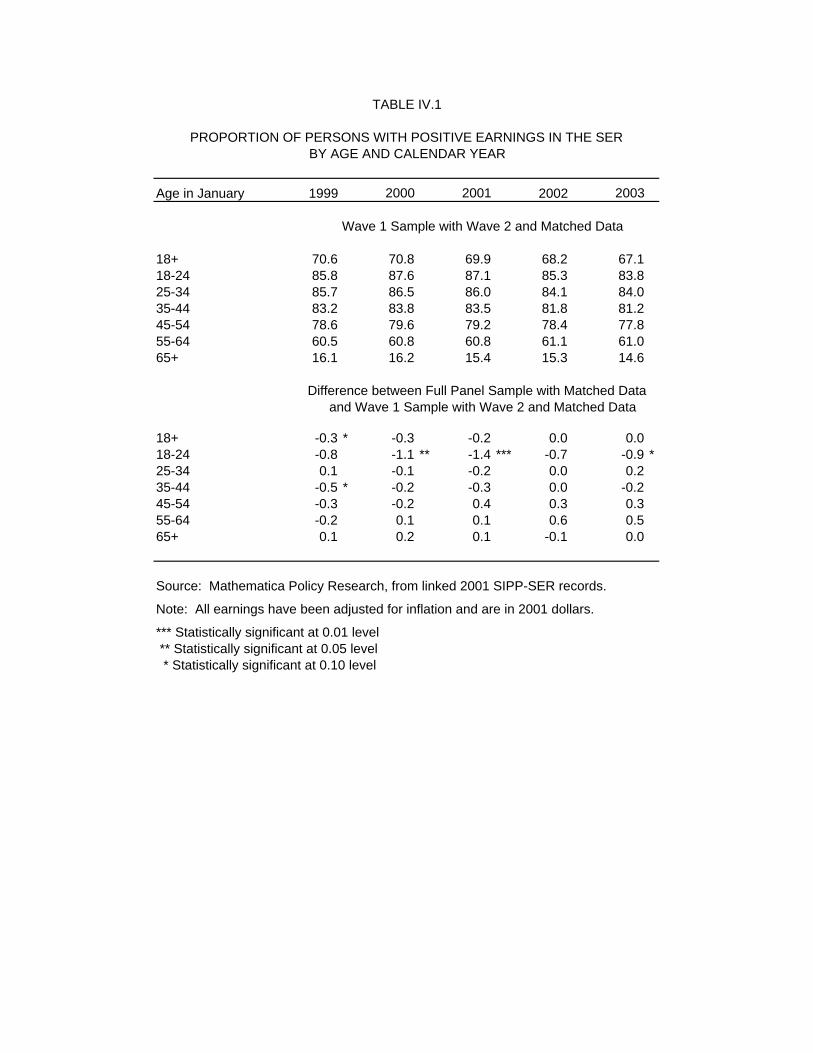
TABLE IV.1

PROPORTION OF PERSONS WITH POSITIVE EARNINGS IN THE SERBY AGE AND CALENDAR YEAR

Age in January 1999 2000 2001 2002 2003

18+ 70.6 70.8 69.9 68.2 67.118-24 85.8 87.6 87.1 85.3 83.825-34 85.7 86.5 86.0 84.1 84.035-44 83.2 83.8 83.5 81.8 81.245-54 78.6 79.6 79.2 78.4 77.855-64 60.5 60.8 60.8 61.1 61.065+ 16.1 16.2 15.4 15.3 14.6

Difference between Full Panel Sample with Matched Dataand Wave 1 Sample with Wave 2 and Matched Data

18+ -0.3 * -0.3 -0.2 0.0 0.0 18-24 -0.8 -1.1 ** -1.4 *** -0.7 -0.9 *25-34 0.1 -0.1 -0.2 0.0 0.2 35-44 -0.5 * -0.2 -0.3 0.0 -0.2 45-54 -0.3 -0.2 0.4 0.3 0.3 55-64 -0.2 0.1 0.1 0.6 0.5 65+ 0.1 0.2 0.1 -0.1 0.0

Source: Mathematica Policy Research, from linked 2001 SIPP-SER records.

Note: All earnings have been adjusted for inflation and are in 2001 dollars.

*** Statistically significant at 0.01 level ** Statistically significant at 0.05 level * Statistically significant at 0.10 level

Wave 1 Sample with Wave 2 and Matched Data

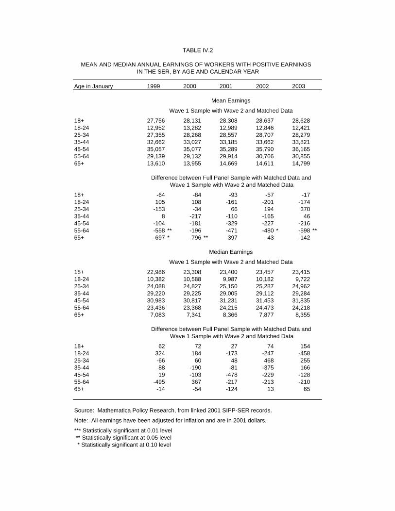
TABLE IV.2

MEAN AND MEDIAN ANNUAL EARNINGS OF WORKERS WITH POSITIVE EARNINGS IN THE SER, BY AGE AND CALENDAR YEAR

Age in January 1999 2000 2001 2002 2003

18+ 27,756 28,131 28,308 28,637 28,62818-24 12,952 13,282 12,989 12,846 12,42125-34 27,355 28,268 28,557 28,707 28,27935-44 32,662 33,027 33,185 33,662 33,82145-54 35,057 35,077 35,289 35,790 36,16555-64 29,139 29,132 29,914 30,766 30,85565+ 13,610 13,955 14,669 14,611 14,799

18+ -64 -84 -93 -57 -17 18-24 105 108 -161 -201 -174 25-34 -153 -34 66 194 370 35-44 8 -217 -110 -165 46 45-54 -104 -181 -329 -227 -216 55-64 -558 ** -196 -471 -480 * -598 **65+ -697 * -796 ** -397 43 -142

18+ 22,986 23,308 23,400 23,457 23,41518-24 10,382 10,588 9,987 10,182 9,72225-34 24,088 24,827 25,150 25,287 24,96235-44 29,220 29,225 29,005 29,112 29,28445-54 30,983 30,817 31,231 31,453 31,83555-64 23,436 23,368 24,215 24,473 24,21865+ 7,083 7,341 8,366 7,877 8,355

18+ 62 72 27 74 154 18-24 324 184 -173 -247 -458 25-34 -66 60 48 468 255 35-44 88 -190 -81 -375 166 45-54 19 -103 -478 -229 -128 55-64 -495 367 -217 -213 -210 65+ -14 -54 -124 13 65

Source: Mathematica Policy Research, from linked 2001 SIPP-SER records.

Note: All earnings have been adjusted for inflation and are in 2001 dollars.

*** Statistically significant at 0.01 level ** Statistically significant at 0.05 level * Statistically significant at 0.10 level

Wave 1 Sample with Wave 2 and Matched Data

Difference between Full Panel Sample with Matched Data and Wave 1 Sample with Wave 2 and Matched Data

Difference between Full Panel Sample with Matched Data and Wave 1 Sample with Wave 2 and Matched Data

Wave 1 Sample with Wave 2 and Matched Data

Mean Earnings

Median Earnings

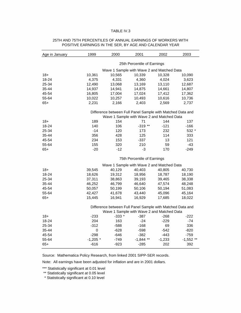
TABLE IV.3

25TH AND 75TH PERCENTILES OF ANNUAL EARNINGS OF WORKERS WITHPOSITIVE EARNINGS IN THE SER, BY AGE AND CALENDAR YEAR

Age in January 1999 2000 2001 2002 2003

18+ 10,361 10,565 10,339 10,328 10,09018-24 4,375 4,331 4,360 4,024 3,62325-34 12,490 13,068 13,169 13,110 12,68735-44 14,937 14,941 14,875 14,661 14,80745-54 16,805 17,004 17,024 17,412 17,36255-64 10,022 10,257 10,493 10,616 10,73665+ 2,231 2,166 2,403 2,569 2,737

18+ 189 154 71 144 137 18-24 140 106 -319 ** -121 -166 25-34 -14 120 173 232 532 *35-44 356 428 125 114 333 45-54 234 153 -337 13 121 55-64 155 320 210 59 -43 65+ -20 -12 -3 170 -249

18+ 39,545 40,129 40,403 40,805 40,73018-24 18,626 19,312 18,956 18,787 18,19025-34 37,311 38,863 39,193 39,465 38,33835-44 46,252 46,799 46,640 47,574 48,24845-54 50,057 50,199 50,106 50,194 51,08355-64 42,427 41,678 43,440 45,096 45,16465+ 15,445 16,941 16,929 17,685 18,022

18+ -233 -333 * -387 -268 -222 18-24 204 163 -24 -229 -74 25-34 -312 -588 -168 69 336 35-44 0 -628 -598 -542 -820 45-54 -298 -646 -382 -443 -759 55-64 -1,205 * -749 -1,844 ** -1,233 -1,552 **65+ -616 -923 -285 202 392

Source: Mathematica Policy Research, from linked 2001 SIPP-SER records.

Note: All earnings have been adjusted for inflation and are in 2001 dollars.

*** Statistically significant at 0.01 level ** Statistically significant at 0.05 level * Statistically significant at 0.10 level

Wave 1 Sample with Wave 2 and Matched Data

Difference between Full Panel Sample with Matched Data and Wave 1 Sample with Wave 2 and Matched Data

Difference between Full Panel Sample with Matched Data and Wave 1 Sample with Wave 2 and Matched Data

Wave 1 Sample with Wave 2 and Matched Data

25th Percentile of Earnings

75th Percentile of Earnings

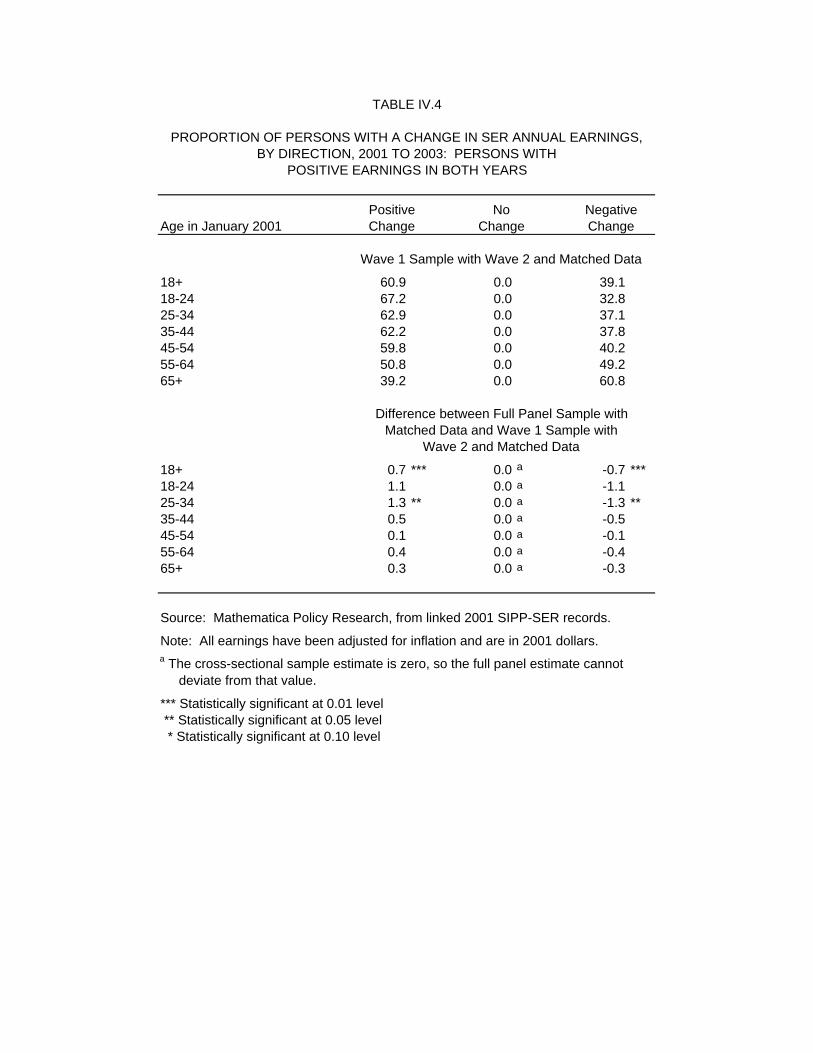
TABLE IV.4

PROPORTION OF PERSONS WITH A CHANGE IN SER ANNUAL EARNINGS,BY DIRECTION, 2001 TO 2003: PERSONS WITH

POSITIVE EARNINGS IN BOTH YEARS

Positive No NegativeAge in January 2001 Change Change Change

Wave 1 Sample with Wave 2 and Matched Data

18+ 60.9 0.0 39.118-24 67.2 0.0 32.825-34 62.9 0.0 37.135-44 62.2 0.0 37.845-54 59.8 0.0 40.255-64 50.8 0.0 49.265+ 39.2 0.0 60.8

Difference between Full Panel Sample withMatched Data and Wave 1 Sample with

Wave 2 and Matched Data

18+ 0.7 *** 0.0 a -0.7 ***18-24 1.1 0.0 a -1.1 25-34 1.3 ** 0.0 a -1.3 **35-44 0.5 0.0 a -0.5 45-54 0.1 0.0 a -0.1 55-64 0.4 0.0 a -0.4 65+ 0.3 0.0 a -0.3

Source: Mathematica Policy Research, from linked 2001 SIPP-SER records.

Note: All earnings have been adjusted for inflation and are in 2001 dollars.a The cross-sectional sample estimate is zero, so the full panel estimate cannot deviate from that value.

*** Statistically significant at 0.01 level ** Statistically significant at 0.05 level * Statistically significant at 0.10 level

TABLE IV.5

FREQUENCY DISTRIBUTION OF GROSS CHANGE IN SER ANNUAL EARNINGS,2001 TO 2003, BY AGE: PERSONS WITH POSITIVE EARNINGS BOTH YEARS

(Thousands of Persons)

Age in January 2001

18+ 18 to 64 65+

Wave 1 Sample with Wave 2 and Matched Data

(More than -25.0%) 23,442 22,182 1,260(-10.1% to -25.0%) 10,556 10,096 460(-5.1% to -10.0%) 6,408 6,225 183(-2.1% to -5.0%) 6,219 5,954 265(-0.1% to -2.0%) 4,397 4,252 145

0 0 0 0(0.1% to 2.0%) 5,001 4,922 79(2.1% to 5.0%) 14,487 14,194 293(5.1% to 10.0%) 11,063 10,889 174(10.1% to 25.0%) 18,030 17,763 267(More than 25.0%) 30,949 30,269 680

Difference between Full Panel Sample withMatched Data and Wave 1 Sample with

Wave 2 and Matched Data

(More than -25.0%) -1,153 *** -1,137 *** -15(-10.1% to -25.0%) -220 -221 1(-5.1% to -10.0%) 145 138 7(-2.1% to -5.0%) 225 233 * -8(-0.1% to -2.0%) 33 21 12

0 0 a 0 a 0 a

(0.1% to 2.0%) 188 192 -4(2.1% to 5.0%) 130 131 -1(5.1% to 10.0%) 530 *** 523 *** 6(10.1% to 25.0%) 235 227 8(More than 25.0%) -393 -401 8

Source: Mathematica Policy Research, from linked 2001 SIPP-SER records.

Note: All earnings have been adjusted for inflation and are in 2001 dollars.a The cross-sectional sample estimate is zero, so the full panel estimate cannot deviate from that value.

*** Statistically significant at 0.01 level ** Statistically significant at 0.05 level

Percentage Change in Earnings

TABLE IV.6

DISTRIBUTION OF SOCIAL SECURITY BENEFICIARY STATUS IDENTIFIED IN THE MBR, BY AGE:JANUARY 2001 AND SEPTEMBER 2003

(Thousands of Persons)

Disabled Retired Aged Aged All OtherAge Worker Worker Non-widow Widow Beneficiaries Total

January 2001: Under 65 5,000 2,620 240 334 3,986 12,180 65 and older 0 25,435 1,720 3,107 21 30,283 Total 5,000 28,055 1,960 3,441 4,007 42,462

September 2003: Under 65 5,895 2,861 117 416 4,145 13,434 65 and older 0 27,190 1,681 3,181 24 32,077 Total 5,895 30,051 1,799 3,597 4,169 45,511

Difference between Full Panel Sample with Matched Data andWave 1 Sample with Wave 2 and Matched Data

January 2001: Under 65 23 29 -18 23 137 193 65 and older 0 a -84 -80 23 0 -141 * Total 23 -56 -99 * 46 138 52

September 2003: Under 65 -65 -48 -18 18 61 -51 65 and older 0 a -284 * -58 -12 0 -354 ** Total -65 -332 ** -75 6 61 -405 *

Source: Mathematica Policy Research, from linked 2001 SIPP-MBR-PHUS records.

Note: The category "all other beneficiaries" includes spouses and widow(er)s caring for minor children, disabled widow(er)s, adults disabled in childhood, student children, minor children, and other individuals who have a current payment status and who are not elsewhere classified.a The cross-sectional sample estimate is zero, so the full panel estimate cannot deviate from that value.

*** Statistically significant at 0.01 level ** Statistically significant at 0.05 level * Statistically significant at 0.10 level

Wave 1 Sample with Wave 2 and Matched Data

TABLE IV.7

ENTRIES INTO AND EXITS FROM SOCIAL SECURITY BENEFICIARY CATEGORIESBETWEEN JANUARY 2001 AND SEPTEMBER 2003

(Thousands of Persons)

Beneficiary January Entries into Exits from SeptemberCategory 2001 Category Category 2003

Wave 1 Sample with Wave 2 and Matched Data

Disabled worker 5,000 1,835 939 5,895Retired worker 28,055 4,559 2,563 30,051Aged non-widow 1,960 194 355 1,799Aged widow 3,441 599 443 3,597All other beneficiaries 4,007 1,330 1,168 4,169

Total 42,462 8,517 5,468 45,511

Difference between Full Panel Sample with Matched Dataand Wave 1 Sample with Wave 2 and Matched Data

Disabled worker 23 -35 52 -65 Retired worker -56 -86 190 ** -332 **Aged non-widow -99 * -11 -34 -75 Aged widow 46 -13 27 6 All other beneficiaries 138 -104 -27 61

Total 52 -249 * 208 -405 *

Source: Mathematica Policy Research, from 2001 linked SIPP-MBR-PHUS records.

Note: The category "all other beneficiaries" includes spouses and widow(er)s caring for minor children, disabled widow(er)s, adults disabled in childhood, student children, minor children, and other individuals who have a current payment status and are not elsewhere classified.

*** Statistically significant at 0.01 level ** Statistically significant at 0.05 level * Statistically significant at 0.10 level

TABLE IV.8

MEAN DOLLAR VALUES OF SELECTED PAYMENT VARIABLES AMONG RETIRED AND DISABLED WORKERS WHO ARE CURRENT BENEFICIARIES, JANUARY 2001 AND SEPTEMBER 2003

January 2001 September 2003

Retired Workers Retired Workers

Under Disabled Under DisabledPayment Variable 65 65+ Total Workers 65 65+ Total Workers

Wave 1 Sample with Wave 2 and Matched Data

Family Maximum Benefit 1,628 1,467 1,482 1,116 1,703 1,481 1,502 1,158Indexed Monthly Earnings 2,069 1,099 1,190 1,178 2,192 1,224 1,316 1,340Monthly Benefit Amount 809 858 854 768 810 867 862 800Monthly Benefit Payable 806 813 812 745 806 817 816 777Medicare Part B Premium 1 45 41 22 2 49 45 23Monthly Benefit Paid 732 810 802 717 755 813 807 816Primary Insurance Amount 953 856 865 775 991 863 876 806Social Security Income 733 855 843 739 757 862 852 838

Difference between Full Panel Sample with Matched Data andWave 1 Sample with Wave 2 and Matched Data

Family Maximum Benefit -1 -7 -6 -1 7 -10 -8 -9Indexed Monthly Earnings -11 -13 -12 -8 12 -14 -12 -13Monthly Benefit Amount -1 -4 -3 0 -2 -6 * -5 * -5Monthly Benefit Payable -1 -3 -3 0 -2 -6 * -5 * -5Medicare Part B Premium 0 0 0 0 0 0 0 0Monthly Benefit Paid -5 -3 -3 17 -1 -6 * -5 * -4Primary Insurance Amount -1 -5 -4 0 4 -6 * -5 * -5Social Security Income -5 -3 -4 17 -1 -6 * -6 * -4

Source: Mathematica Policy Research, from 2001 linked SIPP-MBR-PHUS records.

* Statistically significant at 0.10 level

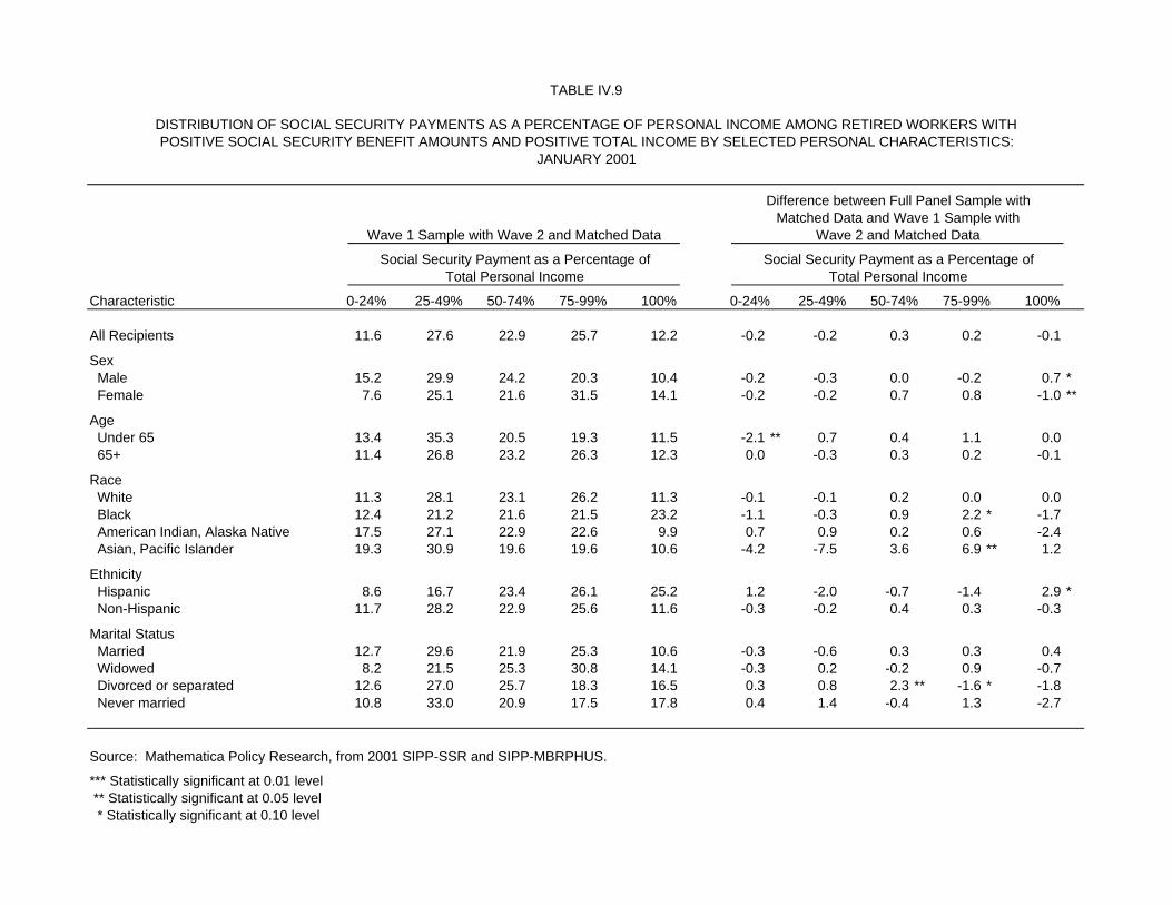
DISTRIBUTION OF SOCIAL SECURITY PAYMENTS AS A PERCENTAGE OF PERSONAL INCOME AMONG RETIRED WORKERS WITHPOSITIVE SOCIAL SECURITY BENEFIT AMOUNTS AND POSITIVE TOTAL INCOME BY SELECTED PERSONAL CHARACTERISTICS:

JANUARY 2001

Difference between Full Panel Sample withMatched Data and Wave 1 Sample with

Wave 1 Sample with Wave 2 and Matched Data Wave 2 and Matched Data

Social Security Payment as a Percentage of Social Security Payment as a Percentage ofTotal Personal Income Total Personal Income

Characteristic 0-24% 25-49% 50-74% 75-99% 100% 0-24% 25-49% 50-74% 75-99% 100%

All Recipients 11.6 27.6 22.9 25.7 12.2 -0.2 -0.2 0.3 0.2 -0.1

Sex Male 15.2 29.9 24.2 20.3 10.4 -0.2 -0.3 0.0 -0.2 0.7 * Female 7.6 25.1 21.6 31.5 14.1 -0.2 -0.2 0.7 0.8 -1.0 **

Age Under 65 13.4 35.3 20.5 19.3 11.5 -2.1 ** 0.7 0.4 1.1 0.0 65+ 11.4 26.8 23.2 26.3 12.3 0.0 -0.3 0.3 0.2 -0.1

Race White 11.3 28.1 23.1 26.2 11.3 -0.1 -0.1 0.2 0.0 0.0 Black 12.4 21.2 21.6 21.5 23.2 -1.1 -0.3 0.9 2.2 * -1.7 American Indian, Alaska Native 17.5 27.1 22.9 22.6 9.9 0.7 0.9 0.2 0.6 -2.4 Asian, Pacific Islander 19.3 30.9 19.6 19.6 10.6 -4.2 -7.5 3.6 6.9 ** 1.2

Ethnicity Hispanic 8.6 16.7 23.4 26.1 25.2 1.2 -2.0 -0.7 -1.4 2.9 * Non-Hispanic 11.7 28.2 22.9 25.6 11.6 -0.3 -0.2 0.4 0.3 -0.3

Marital Status Married 12.7 29.6 21.9 25.3 10.6 -0.3 -0.6 0.3 0.3 0.4 Widowed 8.2 21.5 25.3 30.8 14.1 -0.3 0.2 -0.2 0.9 -0.7 Divorced or separated 12.6 27.0 25.7 18.3 16.5 0.3 0.8 2.3 ** -1.6 * -1.8 Never married 10.8 33.0 20.9 17.5 17.8 0.4 1.4 -0.4 1.3 -2.7

Source: Mathematica Policy Research, from 2001 SIPP-SSR and SIPP-MBRPHUS.

*** Statistically significant at 0.01 level ** Statistically significant at 0.05 level * Statistically significant at 0.10 level

TABLE IV.9

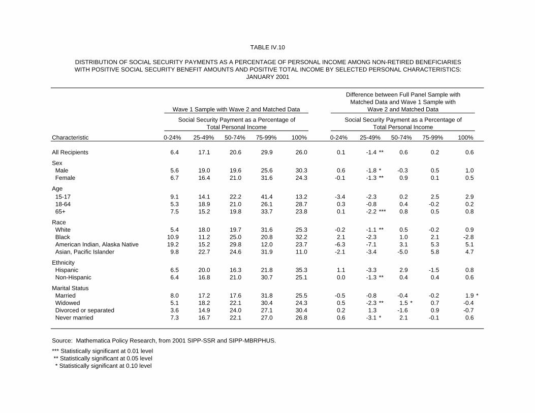
DISTRIBUTION OF SOCIAL SECURITY PAYMENTS AS A PERCENTAGE OF PERSONAL INCOME AMONG NON-RETIRED BENEFICIARIESWITH POSITIVE SOCIAL SECURITY BENEFIT AMOUNTS AND POSITIVE TOTAL INCOME BY SELECTED PERSONAL CHARACTERISTICS:

JANUARY 2001

Difference between Full Panel Sample withMatched Data and Wave 1 Sample with

Wave 1 Sample with Wave 2 and Matched Data Wave 2 and Matched Data

Social Security Payment as a Percentage of Social Security Payment as a Percentage ofTotal Personal Income Total Personal Income

Characteristic 0-24% 25-49% 50-74% 75-99% 100% 0-24% 25-49% 50-74% 75-99% 100%

All Recipients 6.4 17.1 20.6 29.9 26.0 0.1 -1.4 ** 0.6 0.2 0.6

Sex Male 5.6 19.0 19.6 25.6 30.3 0.6 -1.8 * -0.3 0.5 1.0 Female 6.7 16.4 21.0 31.6 24.3 -0.1 -1.3 ** 0.9 0.1 0.5

Age 15-17 9.1 14.1 22.2 41.4 13.2 -3.4 -2.3 0.2 2.5 2.9 18-64 5.3 18.9 21.0 26.1 28.7 0.3 -0.8 0.4 -0.2 0.2 65+ 7.5 15.2 19.8 33.7 23.8 0.1 -2.2 *** 0.8 0.5 0.8

Race White 5.4 18.0 19.7 31.6 25.3 -0.2 -1.1 ** 0.5 -0.2 0.9 Black 10.9 11.2 25.0 20.8 32.2 2.1 -2.3 1.0 2.1 -2.8 American Indian, Alaska Native 19.2 15.2 29.8 12.0 23.7 -6.3 -7.1 3.1 5.3 5.1 Asian, Pacific Islander 9.8 22.7 24.6 31.9 11.0 -2.1 -3.4 -5.0 5.8 4.7

Ethnicity Hispanic 6.5 20.0 16.3 21.8 35.3 1.1 -3.3 2.9 -1.5 0.8 Non-Hispanic 6.4 16.8 21.0 30.7 25.1 0.0 -1.3 ** 0.4 0.4 0.6

Marital Status Married 8.0 17.2 17.6 31.8 25.5 -0.5 -0.8 -0.4 -0.2 1.9 * Widowed 5.1 18.2 22.1 30.4 24.3 0.5 -2.3 ** 1.5 * 0.7 -0.4 Divorced or separated 3.6 14.9 24.0 27.1 30.4 0.2 1.3 -1.6 0.9 -0.7 Never married 7.3 16.7 22.1 27.0 26.8 0.6 -3.1 * 2.1 -0.1 0.6

Source: Mathematica Policy Research, from 2001 SIPP-SSR and SIPP-MBRPHUS.

*** Statistically significant at 0.01 level ** Statistically significant at 0.05 level * Statistically significant at 0.10 level

TABLE IV.10

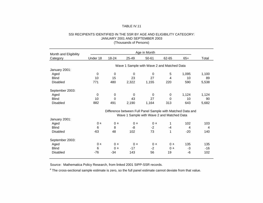
TABLE IV.11

SSI RECIPIENTS IDENTIFIED IN THE SSR BY AGE AND ELIGIBILITY CATEGORY:JANUARY 2001 AND SEPTEMBER 2003

(Thousands of Persons)

Age in Month

Under 18 18-24 25-49 50-61 62-65 65+ Total

Wave 1 Sample with Wave 2 and Matched DataJanuary 2001: Aged 0 0 0 0 5 1,095 1,100 Blind 10 15 23 27 4 10 89 Disabled 771 480 2,322 1,155 220 590 5,538 September 2003: Aged 0 0 0 0 0 1,124 1,124 Blind 10 0 43 27 0 10 90 Disabled 882 491 2,190 1,164 313 643 5,682

Difference between Full Panel Sample with Matched Data and

January 2001: Aged 0 a 0 a 0 a 0 a 1 102 103 Blind 6 8 -8 -2 -4 4 4 Disabled -63 48 102 73 1 -20 140 September 2003: Aged 0 a 0 a 0 a 0 a 0 a 135 135 Blind 6 0 a -17 -2 0 a -3 -16 Disabled -76 -34 143 56 19 -6 102

Source: Mathematica Policy Research, from linked 2001 SIPP-SSR records.a The cross-sectional sample estimate is zero, so the full panel estimate cannot deviate from that value.

Month and Eligibility Category

Wave 1 Sample with Wave 2 and Matched Data

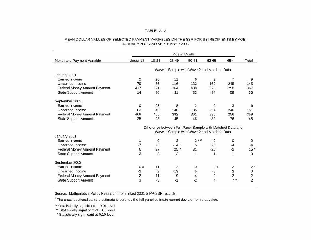
TABLE IV.12

MEAN DOLLAR VALUES OF SELECTED PAYMENT VARIABLES ON THE SSR FOR SSI RECIPIENTS BY AGE:JANUARY 2001 AND SEPTEMBER 2003

Age in Month

Month and Payment Variable Under 18 18-24 25-49 50-61 62-65 65+ Total

Wave 1 Sample with Wave 2 and Matched DataJanuary 2001 Earned Income 2 28 11 6 2 7 9 Unearned Income 79 66 116 133 169 245 145 Federal Money Amount Payment 417 391 364 488 320 258 367 State Support Amount 14 30 31 33 34 58 36

September 2003 Earned Income 0 23 8 2 0 3 6 Unearned Income 63 40 140 135 224 240 151 Federal Money Amount Payment 469 465 382 361 280 256 359 State Support Amount 25 23 45 46 39 76 48

Difference between Full Panel Sample with Matched Data andWave 1 Sample with Wave 2 and Matched Data

January 2001 Earned Income 1 0 3 2 *** -2 0 2 Unearned Income -7 -3 -14 * 5 23 -4 -4 Federal Money Amount Payment 6 27 25 * 31 -20 -2 15 * State Support Amount 2 2 -2 -1 1 1 0

September 2003 Earned Income 0 a 11 2 0 0 a 2 2 * Unearned Income -2 2 -13 5 -5 2 0 Federal Money Amount Payment 2 -11 9 -4 0 -2 -2 State Support Amount 3 -3 -1 -2 4 7 * 2

Source: Mathematica Policy Research, from linked 2001 SIPP-SSR records.a The cross-sectional sample estimate is zero, so the full panel estimate cannot deviate from that value.

*** Statistically significant at 0.01 level ** Statistically significant at 0.05 level * Statistically significant at 0.10 level

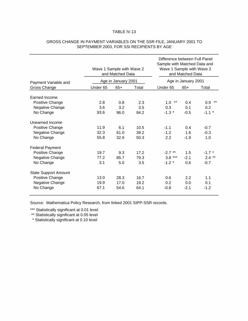
TABLE IV.13

GROSS CHANGE IN PAYMENT VARIABLES ON THE SSR FILE, JANUARY 2001 TOSEPTEMBER 2003, FOR SSI RECIPIENTS BY AGE

Difference between Full PanelSample with Matched Data and

Wave 1 Sample with Wave 2 Wave 1 Sample with Wave 2and Matched Data and Matched Data

Age in January 2001 Age in January 2001

Under 65 65+ Total Under 65 65+ Total

Earned Income Positive Change 2.8 0.8 2.3 1.0 ** 0.4 0.9 ** Negative Change 3.6 3.2 3.5 0.3 0.1 0.2 No Change 93.6 96.0 94.2 -1.3 * -0.5 -1.1 *

Unearned Income Positive Change 11.9 6.1 10.5 -1.1 0.4 -0.7 Negative Change 32.3 61.0 39.2 -1.2 1.6 -0.3 No Change 55.8 32.9 50.3 2.2 -1.9 1.0

Federal Payment Positive Change 19.7 9.3 17.2 -2.7 ** 1.5 -1.7 * Negative Change 77.2 85.7 79.3 3.8 *** -2.1 2.4 ** No Change 3.1 5.0 3.5 -1.2 * 0.6 -0.7

State Support Amount Positive Change 13.0 28.3 16.7 0.6 2.2 1.1 Negative Change 19.9 17.0 19.2 0.2 0.0 0.1 No Change 67.1 54.6 64.1 -0.8 -2.1 -1.2

Source: Mathematica Policy Research, from linked 2001 SIPP-SSR records.

*** Statistically significant at 0.01 level ** Statistically significant at 0.05 level * Statistically significant at 0.10 level

Payment Variable and Gross Change

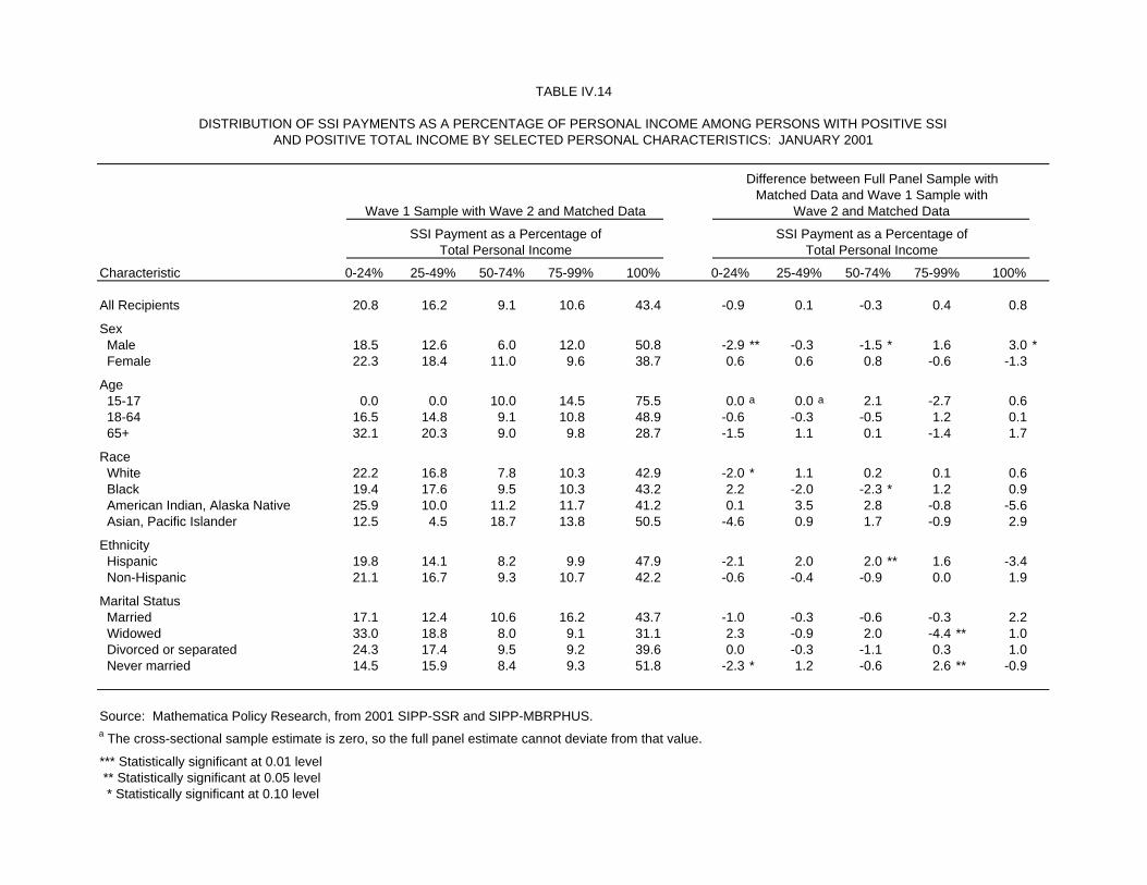
DISTRIBUTION OF SSI PAYMENTS AS A PERCENTAGE OF PERSONAL INCOME AMONG PERSONS WITH POSITIVE SSIAND POSITIVE TOTAL INCOME BY SELECTED PERSONAL CHARACTERISTICS: JANUARY 2001

Difference between Full Panel Sample withMatched Data and Wave 1 Sample with

Wave 1 Sample with Wave 2 and Matched Data Wave 2 and Matched Data

SSI Payment as a Percentage of SSI Payment as a Percentage ofTotal Personal Income Total Personal Income

Characteristic 0-24% 25-49% 50-74% 75-99% 100% 0-24% 25-49% 50-74% 75-99% 100%

All Recipients 20.8 16.2 9.1 10.6 43.4 -0.9 0.1 -0.3 0.4 0.8

Sex Male 18.5 12.6 6.0 12.0 50.8 -2.9 ** -0.3 -1.5 * 1.6 3.0 * Female 22.3 18.4 11.0 9.6 38.7 0.6 0.6 0.8 -0.6 -1.3

Age 15-17 0.0 0.0 10.0 14.5 75.5 0.0 a 0.0 a 2.1 -2.7 0.6 18-64 16.5 14.8 9.1 10.8 48.9 -0.6 -0.3 -0.5 1.2 0.1 65+ 32.1 20.3 9.0 9.8 28.7 -1.5 1.1 0.1 -1.4 1.7

Race White 22.2 16.8 7.8 10.3 42.9 -2.0 * 1.1 0.2 0.1 0.6 Black 19.4 17.6 9.5 10.3 43.2 2.2 -2.0 -2.3 * 1.2 0.9 American Indian, Alaska Native 25.9 10.0 11.2 11.7 41.2 0.1 3.5 2.8 -0.8 -5.6 Asian, Pacific Islander 12.5 4.5 18.7 13.8 50.5 -4.6 0.9 1.7 -0.9 2.9

Ethnicity Hispanic 19.8 14.1 8.2 9.9 47.9 -2.1 2.0 2.0 ** 1.6 -3.4 Non-Hispanic 21.1 16.7 9.3 10.7 42.2 -0.6 -0.4 -0.9 0.0 1.9

Marital Status Married 17.1 12.4 10.6 16.2 43.7 -1.0 -0.3 -0.6 -0.3 2.2 Widowed 33.0 18.8 8.0 9.1 31.1 2.3 -0.9 2.0 -4.4 ** 1.0 Divorced or separated 24.3 17.4 9.5 9.2 39.6 0.0 -0.3 -1.1 0.3 1.0 Never married 14.5 15.9 8.4 9.3 51.8 -2.3 * 1.2 -0.6 2.6 ** -0.9

Source: Mathematica Policy Research, from 2001 SIPP-SSR and SIPP-MBRPHUS.a The cross-sectional sample estimate is zero, so the full panel estimate cannot deviate from that value.

*** Statistically significant at 0.01 level ** Statistically significant at 0.05 level * Statistically significant at 0.10 level

TABLE IV.14

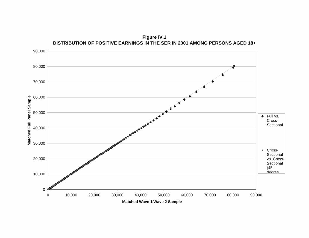
Figure IV.1DISTRIBUTION OF POSITIVE EARNINGS IN THE SER IN 2001 AMONG PERSONS AGED 18+

0

10,000

20,000

30,000

40,000

50,000

60,000

70,000

80,000

90,000

0 10,000 20,000 30,000 40,000 50,000 60,000 70,000 80,000 90,000

Matched Wave 1/Wave 2 Sample

Mat

ched

Fu

ll P

anel

Sam

ple

Full vs.Cross-Sectional

Cross-Sectionalvs. Cross-Sectional(45-degree

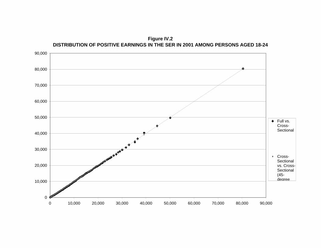
Figure IV.2DISTRIBUTION OF POSITIVE EARNINGS IN THE SER IN 2001 AMONG PERSONS AGED 18-24

0

10,000

20,000

30,000

40,000

50,000

60,000

70,000

80,000

90,000

0 10,000 20,000 30,000 40,000 50,000 60,000 70,000 80,000 90,000

Full vs.Cross-Sectional

Cross-Sectionalvs. Cross-Sectional(45-degree

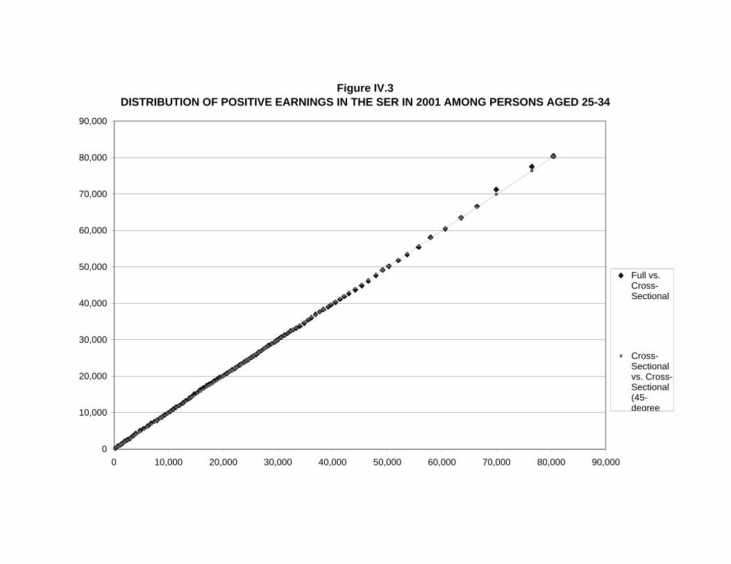
Figure IV.3DISTRIBUTION OF POSITIVE EARNINGS IN THE SER IN 2001 AMONG PERSONS AGED 25-34

0

10,000

20,000

30,000

40,000

50,000

60,000

70,000

80,000

90,000

0 10,000 20,000 30,000 40,000 50,000 60,000 70,000 80,000 90,000

Full vs.Cross-Sectional

Cross-Sectionalvs. Cross-Sectional(45-degree

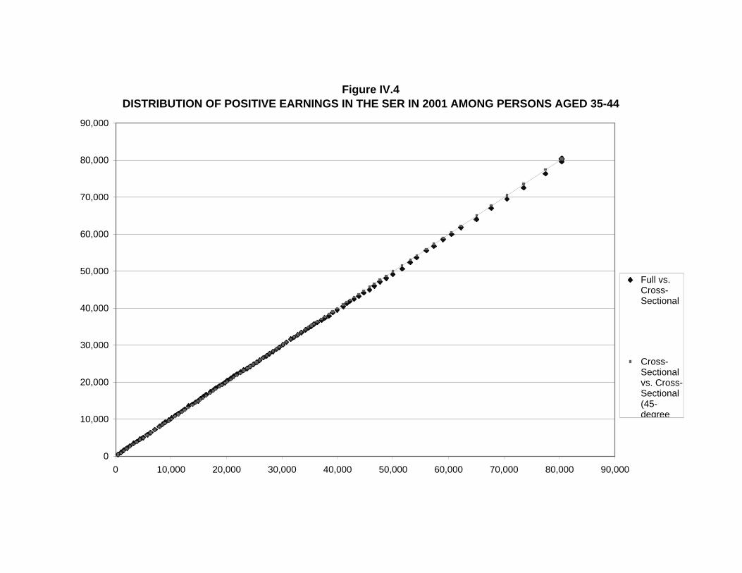
Figure IV.4DISTRIBUTION OF POSITIVE EARNINGS IN THE SER IN 2001 AMONG PERSONS AGED 35-44

0

10,000

20,000

30,000

40,000

50,000

60,000

70,000

80,000

90,000

0 10,000 20,000 30,000 40,000 50,000 60,000 70,000 80,000 90,000

Full vs.Cross-Sectional

Cross-Sectionalvs. Cross-Sectional(45-degree

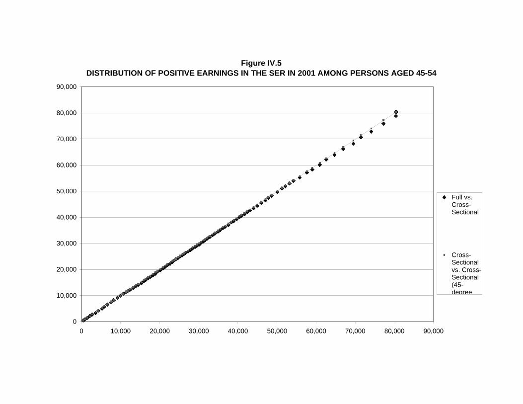
Figure IV.5DISTRIBUTION OF POSITIVE EARNINGS IN THE SER IN 2001 AMONG PERSONS AGED 45-54

0

10,000

20,000

30,000

40,000

50,000

60,000

70,000

80,000

90,000

0 10,000 20,000 30,000 40,000 50,000 60,000 70,000 80,000 90,000

Full vs.Cross-Sectional

Cross-Sectionalvs. Cross-Sectional(45-degree

Figure IV.6DISTRIBUTION OF POSITIVE EARNINGS IN THE SER IN 2001 AMONG PERSONS AGED 55-64

0

10,000

20,000

30,000

40,000

50,000

60,000

70,000

80,000

90,000

0 10,000 20,000 30,000 40,000 50,000 60,000 70,000 80,000 90,000

Matched Wave 1/Wave 2 Sample

Mat

ched

Fu

ll P

anel

Sam

ple

Full vs.Cross-Sectional

Cross-Sectionalvs. Cross-Sectional(45-degree

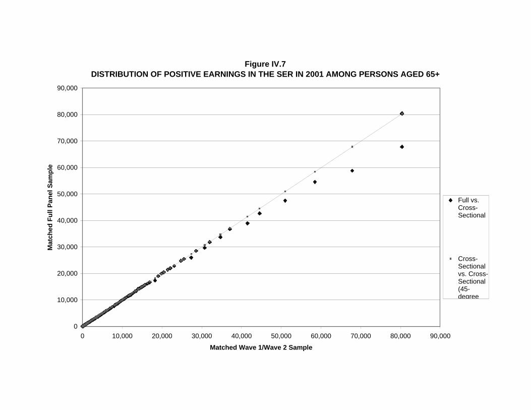
Figure IV.7DISTRIBUTION OF POSITIVE EARNINGS IN THE SER IN 2001 AMONG PERSONS AGED 65+

0

10,000

20,000

30,000

40,000

50,000

60,000

70,000

80,000

90,000

0 10,000 20,000 30,000 40,000 50,000 60,000 70,000 80,000 90,000

Matched Wave 1/Wave 2 Sample

Mat

ched

Fu

ll P

anel

Sam

ple

Full vs.Cross-Sectional

Cross-Sectionalvs. Cross-Sectional(45-degree

133

V. CROSS-SECTIONAL REPRESENTATIVENESS OVER TIME

In order to maintain full cross-sectional representativeness, a panel survey requires two

elements in its design. First, the survey must have a viable mechanism for adding new sample

members to represent additions to the population from which the panel was originally selected.

Second, the survey must have an effective means of compensating for nonrandom attrition. If a

panel survey lacks either of these elements, it will become increasingly less representative of the

full population over time. Recognizing this, designers of panel surveys sometimes employ an

overlapping panel design, in which new panels are started every year, and the data from two or

more panels (depending on the length of the panel) are pooled for cross-sectional estimation. As

long as new panels do not lose their representativeness more rapidly or less rapidly than earlier

panels, the pooled panel estimates derived from data collected at the same time each year will

have a constant bias over time. The SIPP employed an overlapping panel design from 1984

through 1993.1

The loss of cross-sectional representativeness may not be a problem to users interested

solely in longitudinal analysis, providing that the panel accurately represents the original

population through time. In the preceding chapter we presented compelling evidence that the

SIPP full panel sample, when weighted with the Census Bureau’s longitudinal weights, does

indeed provide good representation of the wave 1 population over time—not only for the whole

population but also (and perhaps especially) for subpopulations of Social Security beneficiaries.

But while SSA’s uses of the SIPP include important longitudinal applications, cross-sectional

uses abound. Consequently, the cross-sectional representativeness of the SIPP over time is of

1 The Medical Expenditure Panel Survey continues to employ an overlapping panel design, with two-year

panels being initiated every year. The Medicare Current Beneficiary Survey has an overlapping panel design with four-year panels.

134

considerable interest to SSA analysts. This interest in cross-sectional representativeness extends

to the matched subsample, which SSA analysts have used to examine the characteristics of SSA

beneficiaries at successive points in time.

In this chapter we explore the SIPP’s cross-sectional representativeness over time. We

begin by looking at SSA’s own estimates of the characteristics of disabled workers and SSI

recipients during the final two years of the 1996 panel and the first year of the 2001 panel. Then

we turn our attention to trends in SIPP monthly poverty rates, which raise a number of questions

about the dynamics of the SIPP sample over time and how it affects the cross-sectional estimates

that are derived from the survey. Finally, we look at what the absence of a refreshment

mechanism means with respect to who is missing from SIPP cross-sectional estimates over time,

and, in light of our findings in the previous chapter, we consider whether the lack of a

refreshment mechanism might be the principal source of bias in SIPP cross-sectional estimates.

A. CHARACTERISTICS OF DISABLED WORKERS AND SSI RECIPIENTS

In 2000, SSA began publishing an extensive set of SIPP-based descriptive statistics on the

disabled worker population in the Annual Statistical Report on the Social Security Disability

Insurance Program. This was followed a year later by the initiation of a similar set of statistics

on the SSI population in the SSI Annual Statistical Report. Both sets of statistics were derived

from SIPP data matched to SSA administrative records and were based on data from the third

year of the 1996 panel. Estimates represented the population as of December 1998, with income

corresponding to the 1998 calendar year. Only matched records were used in preparing the

estimates. The matched records were weighted to program beneficiary totals, adjusted to reflect

the noninstitutionalized population. SSA applied the same methodology to produce estimates for

December 1999, with calendar year 1999 income. These estimates were published in the next

volume of each annual report.

135

SSA produced a third set of statistics for each program, based on data from the 2001 SIPP

panel. Because of the reduced match rate attained with this panel, SSA modified the

methodology. Instead of restricting the tabulations to matched records, SSA used both matched

and unmatched records. Beneficiary status and benefit amounts from administrative records

were substituted for reported values on the matched records while reported beneficiary status and

benefit amounts were used for the unmatched records. The tabulations for the DI program

replicated the December reference month and calendar year income used in the earlier tables, so

there was an expectation that the new estimates would line up with the earlier estimates and

provide readers with a glimpse of how the characteristics and economic status of DI beneficiaries

had changed since the end of the 1990s economic boom. And while SSA might have expected

some increase in DI beneficiaries’ reliance upon their Social Security benefits, given the changes

in the economy, including a brief recession in 2001, what the estimates showed was an

improbably large increase in the proportion of their personal and family income that DI

beneficiaries received from Social Security. Later, a careful review of how the estimates were

constructed revealed that most of the increase in personal and family income coming from Social

Security benefits was actually due to the substitution of a different administrative data source for

the one that was used in preparing the 1990s estimates. The new source differed from the earlier

source in how lump sum payments of back benefits were recorded, which gave higher benefits in

the short run to beneficiaries with lump sum payments. Other differences between the two

administrative sources may have existed as well, whereas the impact of differences between the

two SIPP panels and how the data from the two panels were used was unclear.

In producing the 2001 estimates for the SSI program a year later, SSA made other changes

to the methodology. Most notably, the reference period was shifted from December 2001 for

population estimates and the 2001 calendar year for income estimates to the final month of wave

136

2 for the population estimates (May through August 2001, depending on the rotation group) and

the four months of the wave for income estimates (February to May through May to August,

again depending on the rotation group). The change was made with an eye toward a planned,

periodic survey of DI and SSI recipients that involved the administration of a single-wave SIPP

interview to a sample of beneficiaries drawn from program administrative records.2 Because of

this change, the income estimates produced for the 2001 statistical tables are not comparable to

the earlier income estimates from the 1996 panel. Ironically, there was no issue with the

administrative benefit data that replaced the reported Social Security benefits for matched cases.

No additional tabulations were produced. The tables for 2001 were reprinted in the next

year’s editions of the DI and SSI statistical reports, and in the following year SSA announced to

its readers that it had removed the SIPP-based tables from the report because the reduced match

rate and increased attrition had made the estimates too unreliable. At the time of the decision

there was an expectation that SSA would be able to replace the tabulations with equivalent

tabulations from a new and better source—namely, the aforementioned periodic survey of DI and

SSI recipients.

Table V.1 reproduces selected tabulations from the DI tables for all three years, and Table

V.2 reproduces selected tabulations from the SSI tables for the same three years. For disabled

workers the estimates of demographic characteristics are reasonably consistent across the years,

but for health insurance there is a sharp decline in private coverage, which is partially offset by

an increase in reported Medicaid coverage. The income estimates show a sharp decline in the

2 Two of the surveys were carried out, but the first survey had significant omissions from the frame and an

exceedingly low interview rate for child beneficiaries. Both problems were corrected in the second survey, but the Census Bureau’s announced termination of the SIPP resulted in SSA’s cancellation of the third survey, which ultimately could have been fielded but probably without the topical module that was to have collected asset data. Topical modules were dropped for the balance of the 2004 panel when the survey was resumed in wave 9 with half of the wave 8 sample.

137

proportion of DI beneficiaries with Social Security representing less than a quarter of their

personal income. Social Security benefits rise from 36 percent of annual family income in 1999

to 53 percent in 2001 after falling from 45 percent in 1998. Changes in the distribution of family

income relative to the poverty threshold are more modest, however, and generally no greater than

the changes recorded between 1998 and 1999.

We have excluded all of the income-based statistics from the SSI tables presented in Table

V.2 because of the aforementioned change in the length of the reference period. For the

remaining characteristics, overall, the similarities between the 1999 and 2001 estimates are more

striking than the differences, and this is important because December 1999 represents the end of

a four-year panel while May through August of 2001 is near the beginning of a new panel.

Moreover, the estimates of participation in means-tested programs, which we might expect to

show the greatest effects of attrition in the 1996 panel, show lower rather than higher

participation as fuller representation of the population is restored with the 2001 panel.

When we turn from indirect to direct estimates of income, however, we see more clearly the

discontinuity that can develop across SIPP panels, and that is where we focus our attention for

the remainder of this chapter.

B. MONTHLY POVERTY

Estimates of the percentage of persons in poverty by survey month illustrate the

discontinuity between panels that has become a persistent feature of SIPP panels since the 1996

redesign. Each new panel since 1996 has started with a wave 1 poverty rate that was at least two

percentage points higher than the poverty rate in the final wave of the preceding panel (Figure

V.1 and Table V.3).3 This was true even though two of the prior panels—1992 and 2001—

3 We exclude the 1993 panel from this comparison because this panel seems to have drawn a sample with an

over-representation of the low-income population relative to other SIPP panels. Poverty rates in the 1993 panel run

138

showed little if any downward trend over their lifetimes. In fact, the largest difference between

the end of one panel and the beginning of the next—3 percentage points—occurred after the

2001 panel, which showed no decline at all after the second wave.

1. Possible Sources of Discontinuity between Panels

Attrition has been cited as the principal reason that cross-sectional estimates of poverty

might decline over the life of a SIPP panel and then rise when a new panel starts. For example,

Weinberg (2003) observed:

Cross-section estimates from the SIPP are potentially biased by differentially high attrition of low-income households, poverty estimates more than any other. Without refreshment of a panel by new households, as was provided by SIPP’s original (1983) overlapping panel design, poverty estimates would naturally decline over the life of any one panel, jumping up even in the absence of any change in environmental economic conditions when another panel began.

By refreshment Weinberg means the introduction of a new sample that is representative in every

respect rather than just representative of people who have joined the universe since the start of

the previous panel. In fact, Weinberg implies that the biggest contribution of refreshment is to

correct for differential attrition. Our findings in the preceding chapter indicate that the

adjustments for differential attrition that are incorporated into the SIPP longitudinal weights are

effective in eliminating attrition bias in employment, earnings, and receipt of Social Security and

SSI benefits. Is it possible, then, that differential attrition is not really a factor in the

discontinuity between the estimates of poverty at the end of one panel and the beginning of the

next? Could the discontinuity be explained fully by the entrants and re-entrants to the universe,

(continued) about two percentage points higher than they do in the 1992 panel for the same reference months, and participants in the 1993 panel report higher levels of participation in programs serving the low-income population (such as the Food Stamp Program). While part of this difference may reflect the discontinuity that we are discussing, the greater

139

who are not represented and who grow in number between the beginning and end of a panel but

are then fully represented at the start of the next panel? Or is there an attrition bias in the SIPP

cross-sectional weights that is absent from the longitudinal weights? Alternatively, are there one

or more other factors that might contribute to the observed discontinuity, whether or not attrition

plays a role?

One such alternative is “time-in-sample” bias. In the monthly labor force survey that is the

core of the CPS the existence of a time-in-sample bias has been known for decades. Addresses

that are selected into the CPS sample are included in the monthly sample for four consecutive

months, dropped for eight months, and then included again for an additional four months.

Respondents interviewed in the first month report higher unemployment rates than respondents

interviewed in later months. A possible explanation for time-in-sample bias is that respondents

learn to be better respondents over the course of multiple interviews. Earlier interviews tell them

what behaviors they will be expected to report, and they become better observers. Detailed

questions about income recipiency and amounts would seem to lend themselves to such learning

by respondents, with the possible result that respondents provide a more complete report of their

income in successive waves. The Census Bureau has looked for evidence of a time-in-sample

bias in the reporting of income and benefit receipt in the SIPP by comparing data from

overlapping waves in successive panels. This research, conducted prior to the redesign, has

turned up no evidence of a time-in-sample bias in the SIPP (U.S. Census Bureau 1991). With the

abutted panel design, however, it is no longer possible to test for time-in-sample bias in the same

manner, so there are no data on possible time-in-sample bias since the introduction of computer-

assisted interviewing.

(continued) part of the difference appears to be due to the composition of the 1993 panel sample. SIPP staff at the Census

140

While there may be no evidence of time-in-sample bias in earlier SIPP panels, there is a

strong suggestion of some type of correction in the reporting—or perhaps subsequent

processing—of poverty between the first two waves of each SIPP panel since 1996. In each of

the three panels since the redesign, there was at least a one percentage point drop in the estimated

monthly poverty rate between the common reference months of the first and second waves. In

the 2001 panel there was no further reduction in the poverty rate after wave 2. In the 2004 panel

the decline between waves 1 and 2 was close to two percentage points.

We compared poverty status between the first two waves of the 2004 panel to determine

how much of the reduction in poverty could be attributed to sample loss as opposed to actual

change in recorded poverty. We repeated our calculations on waves 2 and 3 to determine how

the gross changes in recorded poverty compared between the two pairs of waves. We found,

first, that more than half of the poor recorded some type of transition between each pair of

waves. Only 20 million out of an estimated 47 million poor persons in wave 1 had no change in

status between waves 1 and 2 while 19 million out of 42 million poor persons in wave 2 had no

change in status (Table V.4). Overall, changes in recorded poverty accounted for 87 percent of

the reduction of 5.0 million poor persons between waves 1 and 2, with sample changes

accounting for the balance.

Between waves 2 and 3, sample changes had a positive effect on the poverty rate—primarily

because of wave 1 sample members who missed the wave 2 interview but returned for wave 3

with family incomes below poverty. As a result, gross changes in poverty accounted for more

than 100 percent of the 0.3 percentage point decline in poverty rates between waves 2 and 3.

The biggest difference between the two pairs of waves, however, lies in the number of persons

(continued) Bureau have acknowledged the uniqueness of the 1993 panel sample.

141

making transitions out of poverty: 14.2 million between waves 1 and 2 versus 11.2 million

between waves 2 and 3. With about the same number making transitions into poverty between

each pair of waves (9.8 million between waves 1 and 2 versus 10.1 million between waves 2 and

3), this difference in the frequency of transitions into poverty drives the final result.

The difference between the two pairs of waves is not dramatic, given the large number of

transitions occurring between both pairs of waves. The difference would be more striking—and

more suggestive of possible causes—if the total number of transitions were significantly smaller

between waves 2 and 3 than between waves 1 and 2. Instead, we see that reported poverty is

quite volatile between both pairs of waves. Nevertheless, transitions out of poverty are

sufficiently more frequent after wave 1 than after wave 2 to yield quite different rates of net

change in poverty. Most likely, only the Census Bureau can determine what accounts for the

difference, but we can be almost certain that the difference does not reflect a markedly greater

incidence of real change between waves 1 and 2 than between waves 2 and 3.

This wave 1 “effect,” as we will identify it subsequently, may be just one manifestation of a

more general development in the SIPP that could also be contributing to the observed

discontinuity between panels. SIPP’s movement to an end-to-end or abutted panel design

increases the extent to which each successive SIPP panel constitutes a different survey. This has

both good and bad implications. The longer time between the start of successive panels (five

years in the case of the 1996 and 2001 panels, although there was a small, abortive 2000 panel)

provides the Census Bureau more time to develop and implement survey innovations, which is

indeed a good thing, generally, although innovations may not always yield better data. At the

same time, however, innovations chip away at the comparability of panels over time. As we will

demonstrate shortly, one particular innovation in the 2004 panel—a genuine improvement—had

a pronounced impact on poverty rates in the subset of the population that the innovation affected.

142

In Chapter VI we will present additional evidence of change across panels that underscores the

point that successive panels are different surveys that cannot be expected to yield strictly

comparable estimates of everything they measure.

2. Discontinuities by Age

There are notable differences across age groups in the magnitudes of the discontinuities

across panels, the sizes of the wave 1 effect, and the within-panel trends (Figures V.2 to V.6).

Both the discontinuity between panels and the wave 1 effect are strongest among young adults

18 to 24—a narrow age group but one that compares in size to the elderly. The discontinuity

grows from 4 percentage points between the end of the 1992 and beginning of the 1996 panel to

5.5 percentage points between the end of the 2001 panel and the beginning of the 2004 panel

(Table V.5). Arguably, the 1992 to 1996 discontinuity is overstated because the monthly poverty

rates in this age group in the comparatively small 1992 panel are highly volatile, with peaks and

troughs that differ by 4.5 percentage points and no discernible trend. The peak, wave 1 value in

the 1996 panel is barely higher than the peaks observed in the 1992 panel. But the lesser

volatility in the 1996 and 2001 panels gives emphasis to the large discontinuities that follow

those two panels. Furthermore, the declines in poverty rates between waves 1 and 2 range from

2.5 to 3.4 percentage points.

Children under 18 and adults 25 to 39 show the most similar patterns over the four panels.

The discontinuities are sharper in the adult group, but both age groups have discernible upward

trends in poverty rates in the 2001 panel and modest wave 1 effects that underscore the extent of

the discontinuity with the 2004 panel. This upward trend in poverty in the 2001 panel is absent

in the 40 to 64 age group, but the break between the 2001 and 2004 panels is the most stark in

this age group, where it stands in sharp contrast to the modest discontinuities and wave 1 effects

observed in the earlier panels. Indeed, the poverty estimates from the first three waves of the

143

2004 panel do not appear to come from the same population as the estimates from the earlier

panels.

The elderly population deviates the most from the other age groups. First, the elderly are

unique in showing an upward trend in poverty in the 1992 panel. Even if we extrapolate this

trend, however, there is still a clear discontinuity with the 1996 panel. Second, the elderly are

also unique in showing a decline in poverty between the end of the 2001 panel and the beginning

of the 2004 panel. More specifically, the estimated poverty rate declined by 1.1 percentage

points between September 2003 and January 2004 whereas it rose by at least 3 percentage points

in every other age group. This is the only instance of a decline in poverty occurring between the

end of one panel and the beginning of the next, and we attribute this result to a change in how

Social Security payment amounts were requested. With the first wave of the 2004 panel, the

SIPP began to measure Social Security payments as a gross amount rather than asking

respondents to exclude the amount of the Medicare Part B premium. The decline in the elderly

poverty rate between September 2003 and January 2004 is evidence that the new procedure

works more effectively than earlier attempts to collect gross payment amounts.4

C. SOURCES OF BIAS IN SIPP CROSS-SECTIONAL ESTIMATES

In the plots of monthly poverty over time, the principal evidence that panels lose their cross-

sectional representativeness over their lifetimes is seen in the discontinuity in poverty estimates

between successive panels rather than the decline in estimated poverty to which Weinberg

alluded. Of the 1992, 1996 and 2001 panels, only the 1996 panel shows a broad-based decline in

4 Unlike earlier attempts to measure gross Social Security payments, which ended after the 1991 panel,

respondents to the 2004 panel are asked to report the amount of their Medicare Part B premiums separately from their benefit payments. Respondents are still asked to report their net payment amounts, but two follow-up questions ask if any deductions are taken out, such as for Medicare Part B premiums, and how much they are. The responses enable the Census Bureau to construct the gross amount.

144

poverty over time, and that panel was fielded during an extended economic boom, from which

there is ample evidence that poverty rates declined significantly. Both the 1992 and 2001 panels

included recessions, so the evidence of declining representativeness may be expressed in

generally flat rather than rising poverty rates. In other words, the tendency for poverty rates to

decline over the life of a SIPP panel may have been offset by an upward secular trend, leaving a

flat trend line as the net result.

The plots of SIPP monthly poverty rates over time also provide evidence that the

discontinuity between panels may be exaggerated by excessive estimates of poverty in the initial

waves of the 1996, 2001 and, especially, 2004 panels. Comparing estimates of poverty between

the final wave of one panel and the second wave of the next panel suggests that the cumulative

bias over the length of a panel may be barely more than a percentage point for the population as

a whole—but two to three percentage points for younger adults.

1. Attrition

The magnitude of attrition in SIPP panels and the voluminous evidence from the SIPP and

other panel surveys that attrition is nonrandom have contributed to a widespread presumption

that differential attrition is the principal source of any discontinuities that may be observed in the

estimates of poverty rates between successive panels. But how can this reconciled with the

findings presented in Chapter IV, showing that the Census Bureau’s full panel weights provide

an effective adjustment for the biasing effects of differential attrition? Could the full panel

weights provide protection against differential attrition while the cross-sectional weights do not?

The non-interview adjustment that is incorporated into the full panel weights is calculated

and applied at the person level while the non-interview adjustment that is built into the cross-

sectional weights is calculated and applied at the household level. This difference reflects the

fact that the cross-sectional non-interview adjustment is calculated independently from one wave

145

to the next. Since data are collected for all members of a sample household in a given wave (or

imputed to those for whom no data can be collected), the same non-interview adjustment is

applied to all members of the same household in a given wave. Because the cross-sectional non-

interview adjustment is calculated and applied at the household level, the adjustment is based on

household-level characteristics, which may include personal characteristics of the household

reference person. The full panel non-interview adjustment is applied at the person level because

sample members who start out in the same household may differ in whether they qualify to

receive full panel weights. Consequently, the full panel non-interview adjustment is based on the

personal characteristics of each respondent who qualifies. Both the cross-sectional and full panel

adjustments are based on characteristics measured in wave 1, however, and both are designed to

minimize differences between all responding wave 1 households or persons and those

households or persons qualifying to receive the post-wave 1 cross-sectional or full panel

longitudinal weights.

Table V.6 compares the characteristics that may be used to define the non-interview

adjustment cells for the full panel and cross-sectional weights. The 149 full panel and 109 cross-

sectional adjustment cells are a small subset of the thousands of possible combinations of

characteristics that would be generated by a full cross-classification of the 10 variables in each

case. The smaller number of cross-sectional than full panel adjustment cells reflects the smaller

number of responding households than responding persons. Could the greater number of

adjustment cells used for the full panel weight make the full panel non-interview adjustment

more effective than the cross-sectional adjustment? Certainly, that is a possibility. At the same

time, however, the fact that the cross-sectional non-interview adjustment is recalculated at each

wave means that the combination of characteristics used to define the 109 adjustment cells can

146

vary from wave to wave, depending on which characteristics—and combinations—best

differentiate between responding and non-responding households at each point.

Several of the characteristics that may be used to define the adjustment cells for the full

panel versus cross-sectional weights are identical, which implies that they are household-level

characteristics. Others, such as poverty level and participation in means-tested programs, are

defined similarly but not identically. Still others—such as whether the respondent was self-

employed or not, or in the labor force or not, and whether the housing unit is owned or rented—

are unique to one or the other weight. We are puzzled by some of these. The full panel non-

interview adjustment potentially includes whether the household was selected from a poverty

stratum or not, but the cross-sectional non-interview adjustment does not. Is this characteristic

really a more effective predictor of response propensity for the full panel than for a given wave,

or does its appearance in one non-interview adjustment but not the other reflect some other

basis? Apart from the different numbers of adjustment cells, however, we see nothing, a priori,

to suggest that the non-interview adjustment for the full panel weight should be more effective

than the adjustment for the cross-sectional weight.

Unfortunately, we cannot evaluate the bias of the weighted cross-sectional sample in the

same way that we could evaluate the bias of the weighted full panel sample. To evaluate the bias

of the full panel sample we compared the subset of wave 1 respondents who received full panel

weights and the complete wave 1 sample from which they were drawn. By using administrative

records matched to both the subsample and the complete sample, we were able to assess

differences at points in time either prior to or subsequent to wave 1. There is no analog for the

cross-sectional sample. The cross-sectional sample in a given wave cannot be compared to a

larger and representative sample of households from which it was drawn, as all of the households

that respond in a given wave receive cross-sectional weights for that wave. Furthermore, the

147

cross-sectional sample is post-stratified to population totals that include persons who are not

represented in the SIPP panel. We have no data on these persons in the SIPP, so we cannot

assess how well the cross-sectional sample compensates for their omission.

We could restrict the comparison to persons who were in the sample in wave 1, by removing

those who entered the sample after wave 1. The point of doing so would be to allow us to assess

the effectiveness of the cross-sectional adjustments for attrition alone. But while we could back

out an approximation of the “mover adjustment” that the Census Bureau builds into the cross-

sectional weights to compensate for the addition of new sample members, we cannot undo the

post-stratification adjustments. Even if we could obtain access to the intermediate cross-

sectional weights, prior to the application of post-stratification, one could argue that these

intermediate weights do not reflect the Census Bureau’s full attrition adjustment and that using

them in an evaluation of attrition bias would understate the effectiveness of the attrition

adjustment.5

If we concede that it is not possible to separate the attrition adjustment from the adjustment

for entries to the population, we can consider an alternative approach to evaluating the cross-

sectional representativeness of a SIPP panel over time. This would involve comparing the SIPP

to an external source—the CPS—using administrative records matched to both samples.

Separate comparisons would be performed between the CPS and SIPP samples in March of each

year, with the weights of the matched records from both surveys being calibrated to the same

population totals. In effect, we would be using administrative records to evaluate the

5 The problem can be explained as follows. If we were adjusting the cross-sectional weights for attrition alone,

we would like to post-stratify the sample weights—after applying the non-interview adjustment—to population totals that reflect the survivors of the population represented by the wave 1 sample. This is important because there are differences in the likelihood of attrition by age, sex, and race/ethnicity. Such population totals do not exist, however. But by post-stratifying the near-final weights to population totals for the whole population, we would simultaneously adjust for demographic differences in attrition and for the sample’s under-representation of persons who entered the population after wave 1.

148

comparability of the two samples in each year, with the presumption that the CPS sample reflects

the true population distribution. The point of using administrative records in the comparison is

to make the comparison independent of the quality of the two surveys’ measures of income and

program participation. We could use SER, MBR, and SSR data to assess whether there are

differences between the two weighted samples and, if so, how the differences change over the

length of a panel.

Differential match bias between the two surveys could be an issue for comparisons done

with administrative records matched to existing panels and CPS files, so it would be better to

conduct such an evaluation using files that were matched to administrative records in the same

way. This will not be possible until the first four or five waves are released from the next SIPP

panel, which is scheduled to enter the field in early 2008.6 Until then, however, it would be

interesting to conduct such an evaluation with the 1996 SIPP panel, which had match rates to

administrative records that were much better than those of the 2001 and 2004 panels and much

closer to those achieved with the corresponding CPS files. We did not include such an

evaluation in this project because it did not provide a way to separate the impact of attrition from

population additions that we have to believe are not well represented. But even though such an

evaluation would speak to only the combined bias from these sources, the documentation of

SIPP longitudinal bias that it would provide would be valuable to SIPP users within SSA and to

the Census Bureau staff that are undertaking a major redesign of the survey.

2. Additions to the Population

In lieu of refreshing the sample with new entrants, the Census Bureau post-stratifies the

cross-sectional weights to estimates of the total population by age, sex, race, and Hispanic origin.

6 It is not possible to evaluate attrition bias until SIPP data for March of the second year are released.

149

This hides the fact that over its lifetime a SIPP panel excludes from representation a growing

proportion of new and returning members of the population—that is, people who were absent

from the survey universe at the start of the panel. These “new” (for short) members of the

population are represented by a SIPP panel only if they join the households of people who were

in the survey universe at the start of the panel. Operationally, they are represented in a SIPP

panel by persons who join SIPP households after having been outside the survey universe in

wave 1.

Births constitute the single largest source of additions to the population at about four million

annually, and while births to young women are substantially underrepresented in the SIPP, the

remaining births are almost fully represented (Czajka and Sykes 2006). The representation of

other additions to the population—which may be as numerous, collectively, as births—is much

less certain. These additions include new and returning immigrants, citizens moving back from

temporary residence abroad, members of the armed forces returning to civilian life, and former

inmates released from institutions, which include prisons as well as medical facilities. We

suspect that these other additions are largely omitted from the SIPP, but the post-stratification of

the cross-sectional sample weights precludes our using the survey data to develop an honest

estimate of the representation of these additions in a SIPP panel sample. This may seem a moot

point if the survey weights sum to the total population—and satisfy detailed population controls

by age, sex, race, and Hispanic origin. But weighting up long-term members of the population to

offset the insufficient number of new members is not a substitute for fuller representation of the

latter and may contribute substantially to the discontinuities that we observe in SIPP poverty

rates across panels.

Using just the longitudinal sample with the full panel weights, we can estimate the number

and characteristics of the survivors of the wave 1 population at the end of the panel. The

150

survivors exclude all people who left the SIPP universe. These include not only decedents but

people who moved out of the country or into institutions or who joined the armed forces and, in

so doing, moved into military barracks or otherwise away from their families. By comparing the

survivors to the cross-sectional sample, which is post-stratified to the total population, we can

estimate the number of gross additions to the population over the length of the panel. These

additions are not represented by the full panel sample, and they give us an outside estimate of the

size of the population that is not represented by the cross-sectional sample as well.

Because births are captured by the panel to a large degree, we assigned full panel weights to

all children born to full panel members after the common month of the first wave of the 1996 and

2001 panels, after first adjusting the weights of new mothers to correct for the under-

representation of young mothers. The weighting adjustments, carried out under two earlier

projects, are documented in Czajka and Sykes (2006) and Castner et al. (2007).

Tables V.7 and V.8 present estimates of the divergence between the full panel and cross-

sectional sample estimates of the November 1999 and September 2003 populations, by age, sex,

race, and Hispanic origin. Overall, the 1996 full panel sample underestimates the November

1999 population by 3.6 percent (4.5 percent for males and 2.8 percent for females) while the

2001 full panel sample underestimates the September 2003 population by 4.0 percent (5.0

percent for males and 3.0 percent for females). The shortfall in 1999 represents 9.9 million

persons compared to 11.4 million in 2003.

The differences between the full panel and cross-sectional sample estimates vary

substantially by age, sex, race and Hispanic origin. In the 1996 panel the shortfall for Hispanic

males is 18 percent compared to 5 percent for black non-Hispanic, less than 2 percent for white

non-Hispanic, and 10 percent for other Hispanic males. The shortfall for Hispanic females is

nearly 17 percent compared to only 2 percent for black non-Hispanic, 0.5 percent for white non-

151

Hispanic and 10 percent for other non-Hispanic females. By age the greatest shortfall occurs

among males 19 to 29, who are underestimated by the panel by 10 percent. Males 30 to 39 are

underestimated by 7 percent while children under 4 are underestimated by 6 percent. We find

the same 6 percent shortfall among females below age 4, but females 19 to 29 are underestimated

by only half as much as their male counterparts at just over 5 percent while females 30 to 39 are

underestimated by less than 5 percent.

Among both sexes the greatest shortfall for any combination of characteristics is found

among Hispanics age 19 to 29. For males the panel underestimates the cross-section by 31

percent. For females the difference is 23 percent. The next biggest group in each sex consists of

Hispanic children 4 to 18. We would not have predicted this from the age-specific patterns, as

the shortfall in this age group is comparatively small overall. But among Hispanic males the

shortfall is 20 percent compared to 17 percent for Hispanic females. Other non-Hispanic males

and females both show large shortfalls among young adults, young children, and adults 62 to 74,

but these differences are derived from small sample sizes, and they are more muted in the 2001

panel.

Lastly, elderly males and females 75 and older are overestimated by both panels, with

differences of 7 and 6 percent among females in the 1996 and 2001 panels, respectively, and

differences of 2 and 3 percent among males. This suggests that among the elderly the SIPP may

retain healthier respondents to a greater degree than less healthy respondents, which results in

lower mortality and perhaps lower rates of institutionalization as well.

The patterns in the 2001 panel are quite similar to those in the 1996 panel, but we see

evidence of large sampling error among minority children under 4, with implausible differences

by sex. That the 9-wave 2001 panel should yield differences as large as the 12-wave 1996 panel

suggests that the volume of additions may have grown. But the population estimates that the

152

Census Bureau used to post-stratify its surveys also became more volatile for a time in the early

2000s with the transition to 2000 census-based controls and the more frequent revision of net

immigration assumptions with the availability of the American Community Survey as a new

source on which to base these assumptions.

Ideally, to assess how the estimated poverty rate is affected by including or excluding these

population additions, we would start with a fully representative sample of the population,

identify all sample member who were outside the survey universe three years earlier, and then

calculate an overall poverty rate for the population with and without these persons.

Unfortunately, neither the SIPP nor the CPS can identify people who have joined the survey

universe since a specified date in the past. Questions on immigration come the closest to doing

this, but these questions ask when the respondent arrived to stay rather than where the respondent

was living at some earlier time period.

Lacking suitable data, we limit the scope of our assessment to asking whether the additions

to the population are sufficiently numerous and distributed in a manner that could feasibly

support the observed shifts in the estimated poverty rate across panels. In other words, could the

poverty rate of the population additions that are not represented in the SIPP be high enough that

their inclusion at the start of the next SIPP panel could raise the overall poverty rate by the

magnitudes seen in Figure V.1?

In the aggregate the answer is yes. At 4 percent of the total population, the omitted

populations would need a collective poverty rate that was 25 percentage points above the overall

poverty rate in order to raise the overall poverty rate by a percentage point. This would imply a

poverty rate of 39 percent, which is well beyond the level observed in any of the age groups in

Figures V.2 through V.6 but not inconceivable for a population dominated by minorities and

153

young adults.7 In earlier work with the 1996 panel, focusing on health insurance coverage, we

found that the proportion of nonelderly persons without health insurance coverage in March

1996 among those with full panel weights was 20 percentage points higher among those who left

the survey universe before the end of the panel than among those who remained in the universe

(Czajka and Sykes 2006). Moreover, large differences were evident even within subgroups

defined by age, sex, and Hispanic origin. In particular, among Hispanic persons 19 to 39, the

uninsured rate among those panel members who remained in the survey universe was 40 percent,

which is very high. Nevertheless, it was 73 percent among the subgroup members who left the

survey universe. We believe that the characteristics of people leaving the survey universe,

except for decedents, tell us something about those who enter the survey universe (apart from

births), because many of those who leave—to go abroad, join the armed forces, or enter

institutions—will eventually return.

While the omitted population could very well account for the discontinuity in poverty rates

observed for the population as a whole, could it also account for the age-specific patterns seen in

Figures V.2 through V.6? For children, there is no issue. One could infer from the poverty

trends in Figure V.2 that there is no discontinuity in poverty rates among children other than

what can be explained by the wave 1 effect. For young adults the omitted group is 7.5 percent of

the population (averaged between the two sexes) in November 1999 and 9.5 percent in

September 2003. At this magnitude, it would take only a 10 percentage point higher poverty rate

to increase the age-group poverty rate by a percentage point. Now, in Figure V.3 the shift in

poverty rates between panels that cannot be attributed to the wave 1 effect is between 2 and 3

percentage points. But given the size of the omitted population in this age group, a poverty rate

7 From the estimated size of the omitted population underlying our estimates in tables V.7 and V.8, we

determined that minorities and young adults 19 to 29 accounted for 86 percent of the omitted population in November 1999 and 88 percent in September 2003.

154

high enough to produce a shift of this magnitude is as plausible as it is for the population as a

whole.

Adults 25 to 39 show discontinuities between panels that are only half as large as those

among younger adults after taking account of a sizable wave 1 effect, and the omitted population

at 6 percent of the population in this age group is certainly large enough that its inclusion could

boost the age group poverty rate by 1 to 1.5 percentage points. Adults 40 to 64 are the most

problematic. The omitted group is only 2 to 3 percent of the age group population, but the

upward shift in the poverty rate is easily a percentage point between the 1996 and 2001 panels

and close to 2 percentage points between the 2001 and 2004 panels after taking account of the

wave 1 effect. An omitted group representing only 3 percent of the population would require a

poverty rate 66 percentage points higher than the rest of the population to raise the age group

poverty rate by 2 percentage points. We find that implausible in this age group. At the same

time, however, the upswing in poverty rates between the 2001 and 2004 panels shown in Figure

V.5 also lacks plausibility even after dismissing the wave 1 poverty rate.

Finally, with the elderly there are too many whites of both sexes and too many black women

represented in the panel, which means that the start of a new panel will reduce rather than

increase their numbers. Discontinuity between panels does not seem to be an issue with the

elderly in the 1996 and 2001 panels, and we have already discussed the impact of the shift to

gross rather than net Social Security payments. A large upward shift in poverty between the

1992 and 1996 panels is left unexplained, but attrition seems an unlikely candidate to explain

that shift, given that attrition is very low among the elderly.

In sum, this brief exercise was intended to make the point that the additions to the

population that are omitted from a panel become large enough over time that when they are

introduced into the SIPP sample at the start of the next panel, they could shift the poverty rate by

155

a sufficient margin to explain the discontinuity that we observe between the end of one panel and

the next. To do so, they would have to have a substantially higher poverty rate than the rest of

the population within their respective age groups. Given that many of the omitted people are

recent immigrants, this is certainly plausible, and we pointed to our experience with health

insurance coverage to support this point. Further work will be required to move this discussion

from speculation about what is plausible to a demonstration of what is the reality.

D. CONCLUSION

While estimates of non-income-related characteristics of disabled workers and SSI

recipients show high levels of consistency across the 1996 and 2001 SIPP panels, this is not true

of poverty estimates, which show marked discontinuities that vary by age. These discontinuities

have been attributed to the cumulative effects of attrition within a panel. While only one of the

last three SIPP panels shows declining poverty estimates over time, each panel has started with a

markedly higher poverty rate than the previous one. Upon exploring this phenomenon further,

however, we find that we can attribute a substantial portion of the discontinuity to a tendency for

SIPP panels since 1996 to obtain high estimates of poverty in the first wave, which then decline

sharply in the second wave. Much of the remaining discontinuity could be due to a phenomenon

which has been largely overlooked in assessments of the representativeness of panel surveys

over time—namely, the bias arising from the general lack of representation of new entrants to the

population. Our evidence of the potential bias resulting from this source is indirect at best, but

we establish the more general point that the new entrants who are excluded from a panel over

time constitute a distinctive group that is large enough and potentially unique enough to induce

marked shifts in poverty when they are suddenly represented in full by a new panel.

In the next chapter we focus more sharply on the income component of poverty estimates.

In doing so we bring in an external source, the CPS, and compare estimates of income receipt

156

and income amounts in the SIPP and CPS over time. The objective is to shed some light on

comparative trends in the two surveys over a period that spans significant innovations in both

surveys and a secular decline in respondents’ willingness to report their income to survey

interviewers.

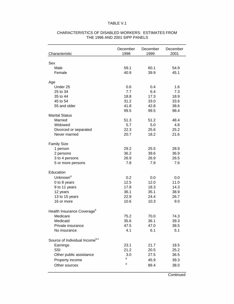
TABLE V.1

CHARACTERISTICS OF DISABLED WORKERS: ESTIMATES FROMTHE 1996 AND 2001 SIPP PANELS

December December DecemberCharacteristic 1998 1999 2001

SexMale 59.1 60.1 54.9Female 40.9 39.9 45.1

AgeUnder 25 0.6 0.4 1.625 to 34 7.7 6.4 7.335 to 44 18.8 17.3 18.945 to 54 31.2 33.0 33.655 and older 41.8 42.8 38.6

99.5 99.5 98.4Marital Status

Married 51.3 51.2 48.4Widowed 5.7 5.0 4.8Divorced or separated 22.3 25.6 25.2Never married 20.7 18.2 21.6

Family Size1 person 29.2 25.5 28.92 persons 36.2 39.6 36.93 to 4 persons 26.9 26.9 26.55 or more persons 7.8 7.9 7.6

EducationUnknowna 0.2 0.0 0.00 to 8 years 12.5 12.0 11.09 to 11 years 17.8 18.3 14.312 years 36.1 35.1 38.913 to 15 years 22.9 24.4 26.716 or more 10.6 10.3 9.0

Health Insurance Coverageb

Medicare 75.2 70.0 74.3Medicaid 35.6 36.1 39.3Private insurance 47.5 47.0 38.5No insurance 4.1 6.1 5.1

Source of Individual Incomeb,c

Earnings 23.1 21.7 18.5SSI 21.2 20.5 25.2Other public assistance 3.0 27.5 36.5Property income d 45.9 39.3Other sources d 89.4 38.0

Continued

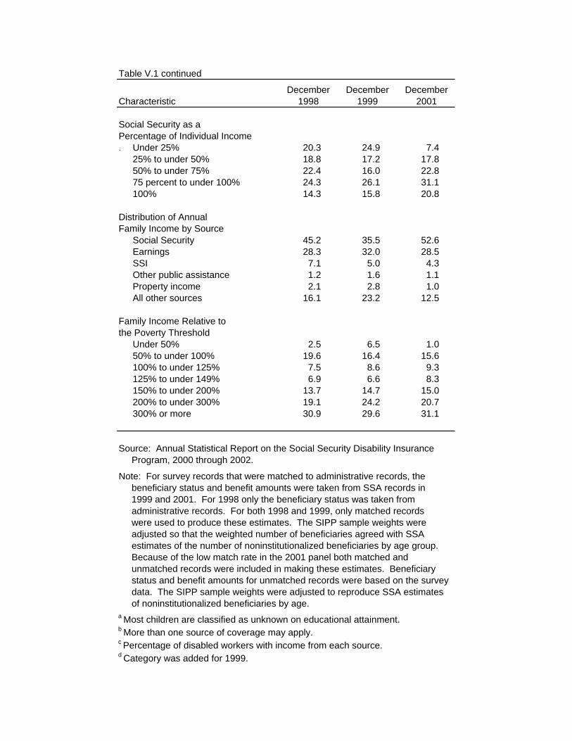
Table V.1 continued

December December DecemberCharacteristic 1998 1999 2001

Social Security as aPercentage of Individual Income. Under 25% 20.3 24.9 7.4

25% to under 50% 18.8 17.2 17.850% to under 75% 22.4 16.0 22.875 percent to under 100% 24.3 26.1 31.1100% 14.3 15.8 20.8

Distribution of AnnualFamily Income by Source

Social Security 45.2 35.5 52.6Earnings 28.3 32.0 28.5SSI 7.1 5.0 4.3Other public assistance 1.2 1.6 1.1Property income 2.1 2.8 1.0All other sources 16.1 23.2 12.5

Family Income Relative tothe Poverty Threshold

Under 50% 2.5 6.5 1.050% to under 100% 19.6 16.4 15.6100% to under 125% 7.5 8.6 9.3125% to under 149% 6.9 6.6 8.3150% to under 200% 13.7 14.7 15.0200% to under 300% 19.1 24.2 20.7300% or more 30.9 29.6 31.1

Source: Annual Statistical Report on the Social Security Disability Insurance Program, 2000 through 2002.

Note: For survey records that were matched to administrative records, the beneficiary status and benefit amounts were taken from SSA records in 1999 and 2001. For 1998 only the beneficiary status was taken from administrative records. For both 1998 and 1999, only matched records were used to produce these estimates. The SIPP sample weights were adjusted so that the weighted number of beneficiaries agreed with SSA estimates of the number of noninstitutionalized beneficiaries by age group. Because of the low match rate in the 2001 panel both matched and unmatched records were included in making these estimates. Beneficiary status and benefit amounts for unmatched records were based on the survey data. The SIPP sample weights were adjusted to reproduce SSA estimates of noninstitutionalized beneficiaries by age.a Most children are classified as unknown on educational attainment.b More than one source of coverage may apply.c Percentage of disabled workers with income from each source.d Category was added for 1999.

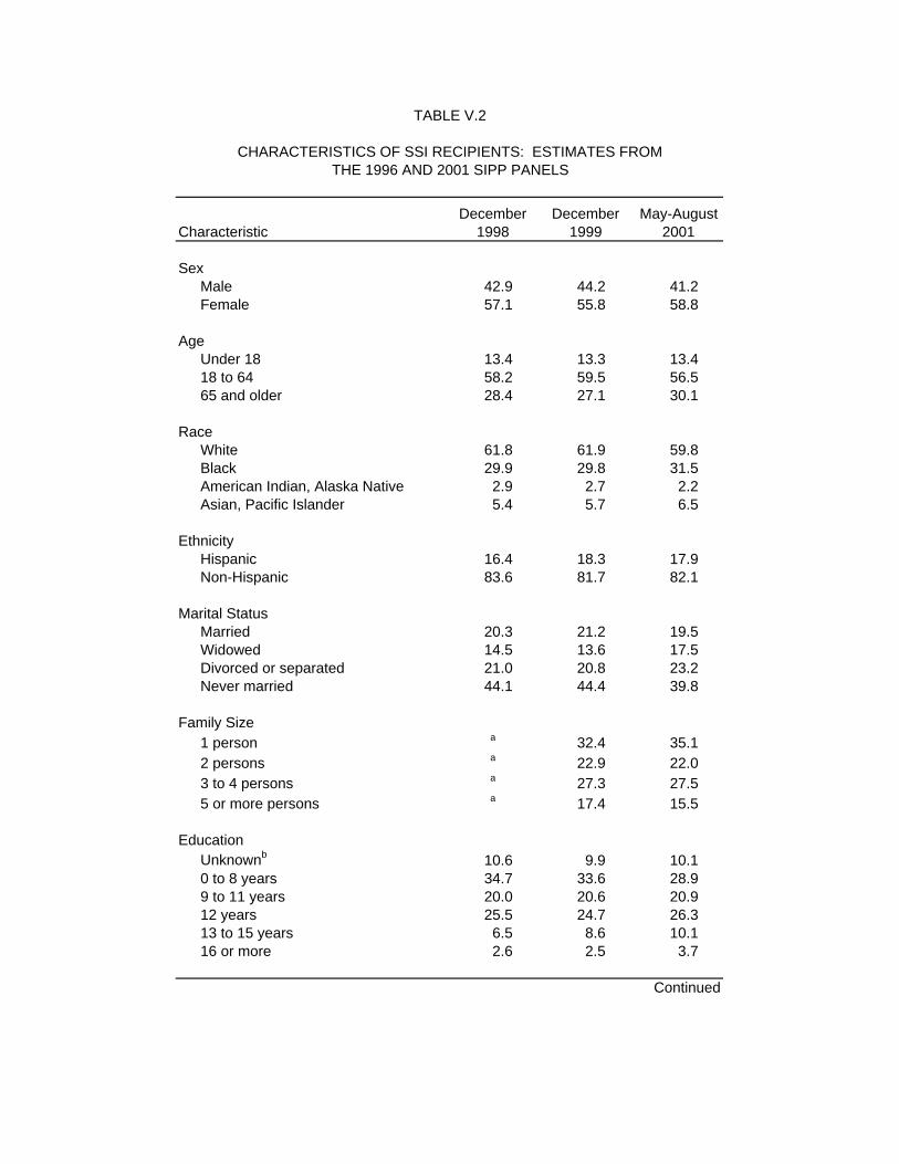
TABLE V.2

CHARACTERISTICS OF SSI RECIPIENTS: ESTIMATES FROMTHE 1996 AND 2001 SIPP PANELS

December December May-AugustCharacteristic 1998 1999 2001

SexMale 42.9 44.2 41.2Female 57.1 55.8 58.8

AgeUnder 18 13.4 13.3 13.418 to 64 58.2 59.5 56.565 and older 28.4 27.1 30.1

RaceWhite 61.8 61.9 59.8Black 29.9 29.8 31.5American Indian, Alaska Native 2.9 2.7 2.2Asian, Pacific Islander 5.4 5.7 6.5

EthnicityHispanic 16.4 18.3 17.9Non-Hispanic 83.6 81.7 82.1

Marital StatusMarried 20.3 21.2 19.5Widowed 14.5 13.6 17.5Divorced or separated 21.0 20.8 23.2Never married 44.1 44.4 39.8

Family Size1 person a 32.4 35.12 persons a 22.9 22.03 to 4 persons a 27.3 27.55 or more persons a 17.4 15.5

EducationUnknownb 10.6 9.9 10.10 to 8 years 34.7 33.6 28.99 to 11 years 20.0 20.6 20.912 years 25.5 24.7 26.313 to 15 years 6.5 8.6 10.116 or more 2.6 2.5 3.7

Continued

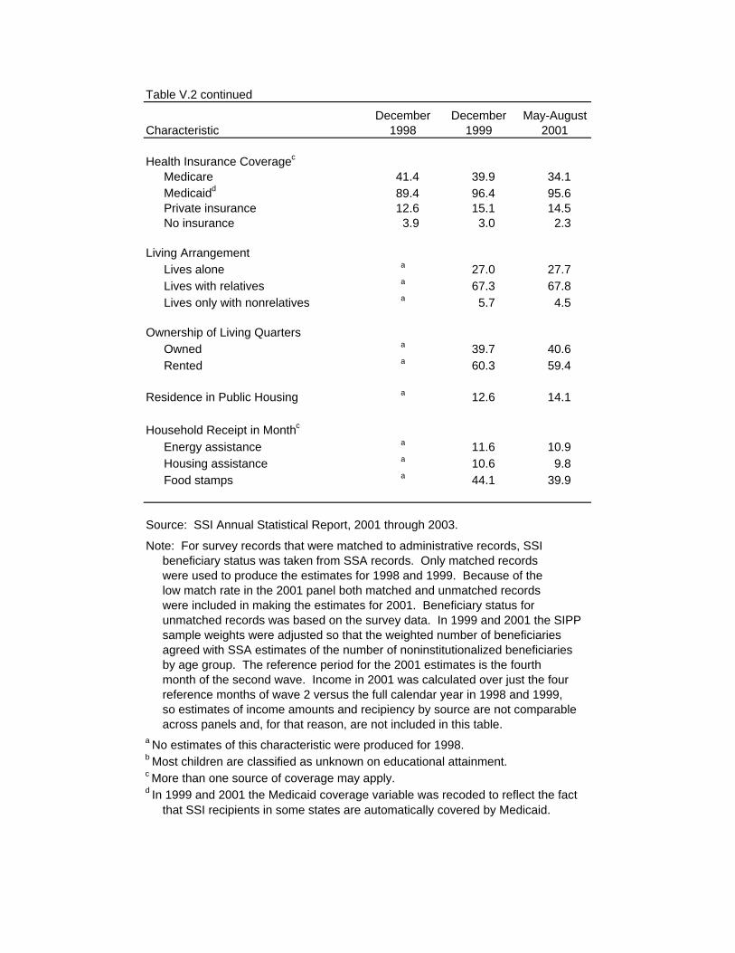
Table V.2 continued

December December May-AugustCharacteristic 1998 1999 2001

Health Insurance Coveragec

Medicare 41.4 39.9 34.1Medicaidd 89.4 96.4 95.6Private insurance 12.6 15.1 14.5No insurance 3.9 3.0 2.3

Living ArrangementLives alone a 27.0 27.7Lives with relatives a 67.3 67.8Lives only with nonrelatives a 5.7 4.5

Ownership of Living QuartersOwned a 39.7 40.6Rented a 60.3 59.4

Residence in Public Housing a 12.6 14.1

Household Receipt in Monthc

Energy assistance a 11.6 10.9Housing assistance a 10.6 9.8Food stamps a 44.1 39.9

Source: SSI Annual Statistical Report, 2001 through 2003.

Note: For survey records that were matched to administrative records, SSI beneficiary status was taken from SSA records. Only matched records were used to produce the estimates for 1998 and 1999. Because of the low match rate in the 2001 panel both matched and unmatched records were included in making the estimates for 2001. Beneficiary status for unmatched records was based on the survey data. In 1999 and 2001 the SIPP sample weights were adjusted so that the weighted number of beneficiaries agreed with SSA estimates of the number of noninstitutionalized beneficiaries by age group. The reference period for the 2001 estimates is the fourth month of the second wave. Income in 2001 was calculated over just the four reference months of wave 2 versus the full calendar year in 1998 and 1999, so estimates of income amounts and recipiency by source are not comparable across panels and, for that reason, are not included in this table.a No estimates of this characteristic were produced for 1998.b Most children are classified as unknown on educational attainment.c More than one source of coverage may apply.d In 1999 and 2001 the Medicaid coverage variable was recoded to reflect the fact that SSI recipients in some states are automatically covered by Medicaid.

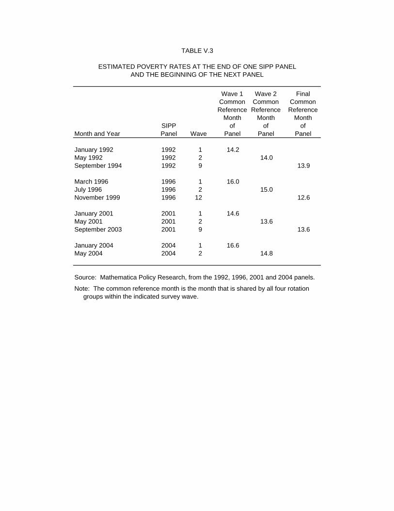
TABLE V.3

ESTIMATED POVERTY RATES AT THE END OF ONE SIPP PANELAND THE BEGINNING OF THE NEXT PANEL

Wave 1 Wave 2 FinalCommon Common CommonReference Reference Reference

Month Month MonthSIPP of of of

Month and Year Panel Wave Panel Panel Panel

January 1992 1992 1 14.2May 1992 1992 2 14.0September 1994 1992 9 13.9

March 1996 1996 1 16.0July 1996 1996 2 15.0November 1999 1996 12 12.6

January 2001 2001 1 14.6May 2001 2001 2 13.6September 2003 2001 9 13.6

January 2004 2004 1 16.6May 2004 2004 2 14.8

Source: Mathematica Policy Research, from the 1992, 1996, 2001 and 2004 panels.

Note: The common reference month is the month that is shared by all four rotation groups within the indicated survey wave.

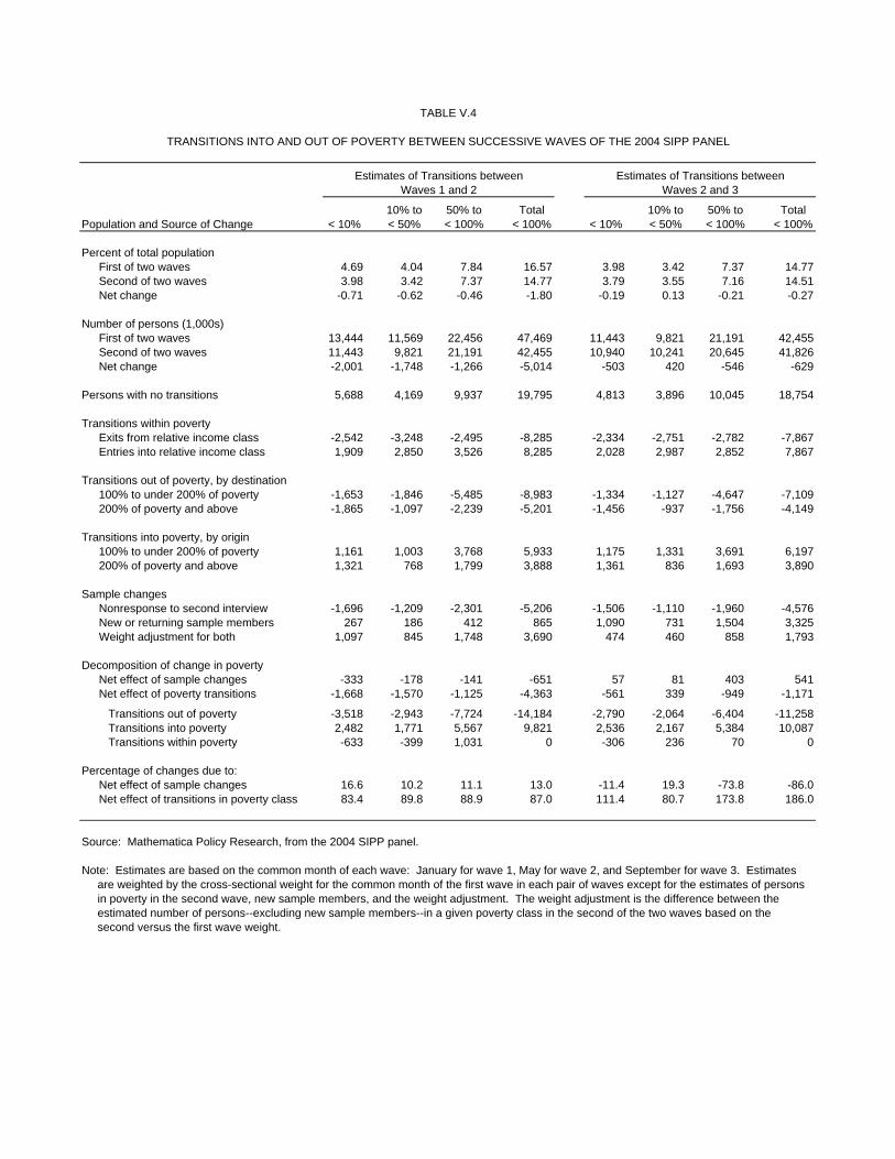
TABLE V.4

TRANSITIONS INTO AND OUT OF POVERTY BETWEEN SUCCESSIVE WAVES OF THE 2004 SIPP PANEL

Estimates of Transitions between Estimates of Transitions betweenWaves 1 and 2 Waves 2 and 3

10% to 50% to Total 10% to 50% to TotalPopulation and Source of Change < 10% < 50% < 100% < 100% < 10% < 50% < 100% < 100%

Percent of total populationFirst of two waves 4.69 4.04 7.84 16.57 3.98 3.42 7.37 14.77Second of two waves 3.98 3.42 7.37 14.77 3.79 3.55 7.16 14.51Net change -0.71 -0.62 -0.46 -1.80 -0.19 0.13 -0.21 -0.27

Number of persons (1,000s)First of two waves 13,444 11,569 22,456 47,469 11,443 9,821 21,191 42,455Second of two waves 11,443 9,821 21,191 42,455 10,940 10,241 20,645 41,826Net change -2,001 -1,748 -1,266 -5,014 -503 420 -546 -629

Persons with no transitions 5,688 4,169 9,937 19,795 4,813 3,896 10,045 18,754

Transitions within povertyExits from relative income class -2,542 -3,248 -2,495 -8,285 -2,334 -2,751 -2,782 -7,867Entries into relative income class 1,909 2,850 3,526 8,285 2,028 2,987 2,852 7,867

Transitions out of poverty, by destination100% to under 200% of poverty -1,653 -1,846 -5,485 -8,983 -1,334 -1,127 -4,647 -7,109200% of poverty and above -1,865 -1,097 -2,239 -5,201 -1,456 -937 -1,756 -4,149

Transitions into poverty, by origin100% to under 200% of poverty 1,161 1,003 3,768 5,933 1,175 1,331 3,691 6,197200% of poverty and above 1,321 768 1,799 3,888 1,361 836 1,693 3,890

Sample changesNonresponse to second interview -1,696 -1,209 -2,301 -5,206 -1,506 -1,110 -1,960 -4,576New or returning sample members 267 186 412 865 1,090 731 1,504 3,325Weight adjustment for both 1,097 845 1,748 3,690 474 460 858 1,793

Decomposition of change in povertyNet effect of sample changes -333 -178 -141 -651 57 81 403 541Net effect of poverty transitions -1,668 -1,570 -1,125 -4,363 -561 339 -949 -1,171

Transitions out of poverty -3,518 -2,943 -7,724 -14,184 -2,790 -2,064 -6,404 -11,258 Transitions into poverty 2,482 1,771 5,567 9,821 2,536 2,167 5,384 10,087 Transitions within poverty -633 -399 1,031 0 -306 236 70 0

Percentage of changes due to:Net effect of sample changes 16.6 10.2 11.1 13.0 -11.4 19.3 -73.8 -86.0Net effect of transitions in poverty class 83.4 89.8 88.9 87.0 111.4 80.7 173.8 186.0

Source: Mathematica Policy Research, from the 2004 SIPP panel.

Note: Estimates are based on the common month of each wave: January for wave 1, May for wave 2, and September for wave 3. Estimates are weighted by the cross-sectional weight for the common month of the first wave in each pair of waves except for the estimates of persons in poverty in the second wave, new sample members, and the weight adjustment. The weight adjustment is the difference between the estimated number of persons--excluding new sample members--in a given poverty class in the second of the two waves based on the second versus the first wave weight.

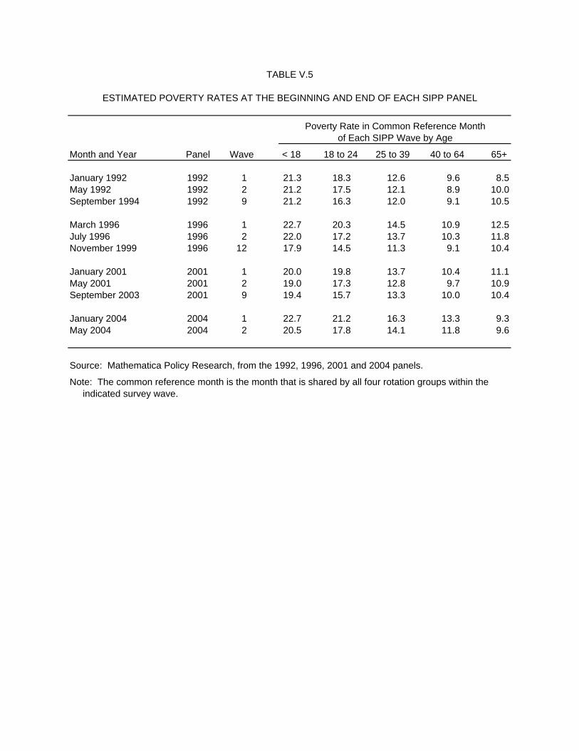
TABLE V.5

ESTIMATED POVERTY RATES AT THE BEGINNING AND END OF EACH SIPP PANEL

Poverty Rate in Common Reference Monthof Each SIPP Wave by Age

Month and Year Panel Wave < 18 18 to 24 25 to 39 40 to 64 65+

January 1992 1992 1 21.3 18.3 12.6 9.6 8.5May 1992 1992 2 21.2 17.5 12.1 8.9 10.0September 1994 1992 9 21.2 16.3 12.0 9.1 10.5

March 1996 1996 1 22.7 20.3 14.5 10.9 12.5July 1996 1996 2 22.0 17.2 13.7 10.3 11.8November 1999 1996 12 17.9 14.5 11.3 9.1 10.4

January 2001 2001 1 20.0 19.8 13.7 10.4 11.1May 2001 2001 2 19.0 17.3 12.8 9.7 10.9September 2003 2001 9 19.4 15.7 13.3 10.0 10.4

January 2004 2004 1 22.7 21.2 16.3 13.3 9.3May 2004 2004 2 20.5 17.8 14.1 11.8 9.6

Source: Mathematica Policy Research, from the 1992, 1996, 2001 and 2004 panels.

Note: The common reference month is the month that is shared by all four rotation groups within the indicated survey wave.

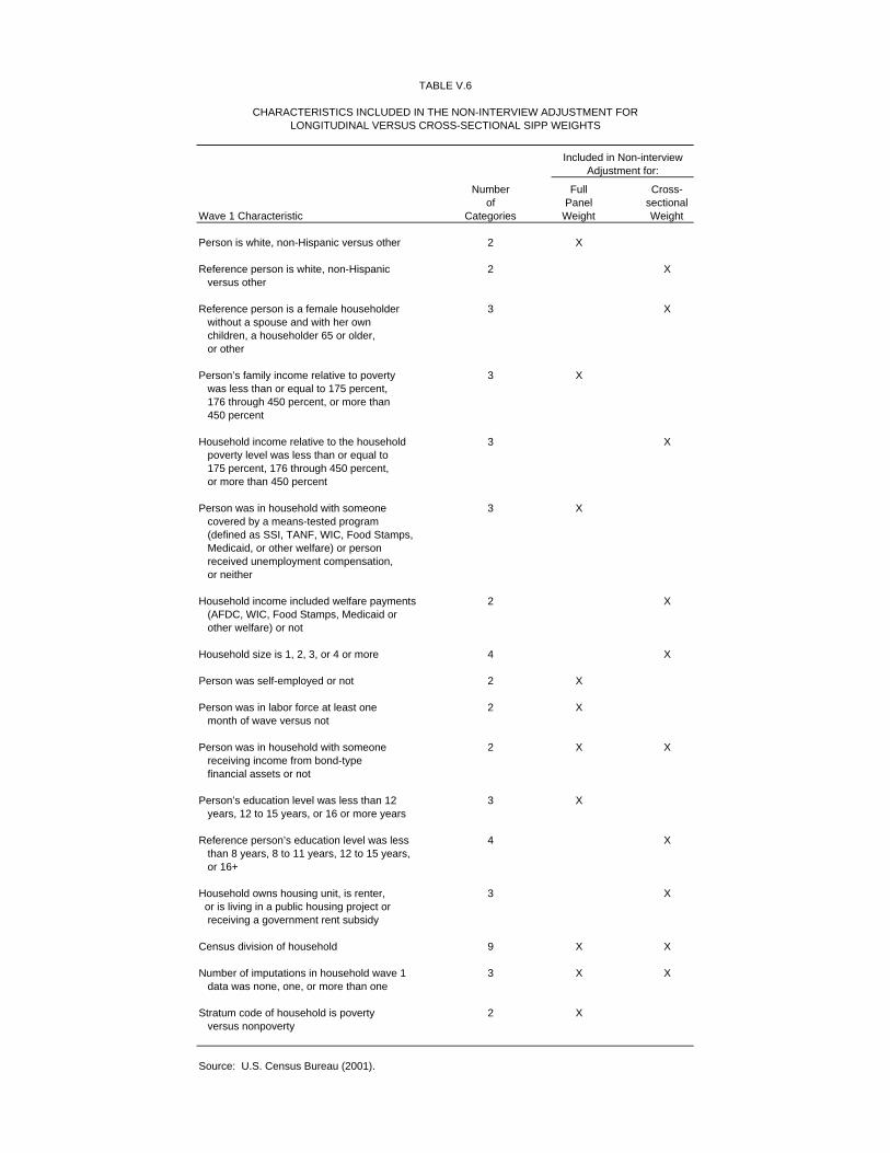
TABLE V.6

CHARACTERISTICS INCLUDED IN THE NON-INTERVIEW ADJUSTMENT FORLONGITUDINAL VERSUS CROSS-SECTIONAL SIPP WEIGHTS

Included in Non-interviewAdjustment for:

Number Full Cross-of Panel sectional

Wave 1 Characteristic Categories Weight Weight

Person is white, non-Hispanic versus other 2 X

Reference person is white, non-Hispanic 2 X versus other

Reference person is a female householder 3 X without a spouse and with her own children, a householder 65 or older, or other

Person’s family income relative to poverty 3 X was less than or equal to 175 percent, 176 through 450 percent, or more than 450 percent

Household income relative to the household 3 X poverty level was less than or equal to 175 percent, 176 through 450 percent, or more than 450 percent

Person was in household with someone 3 X covered by a means-tested program (defined as SSI, TANF, WIC, Food Stamps, Medicaid, or other welfare) or person received unemployment compensation, or neither

Household income included welfare payments 2 X (AFDC, WIC, Food Stamps, Medicaid or other welfare) or not

Household size is 1, 2, 3, or 4 or more 4 X

Person was self-employed or not 2 X

Person was in labor force at least one 2 X month of wave versus not

Person was in household with someone 2 X X receiving income from bond-type financial assets or not

Person’s education level was less than 12 3 X years, 12 to 15 years, or 16 or more years

Reference person’s education level was less 4 X than 8 years, 8 to 11 years, 12 to 15 years, or 16+

Household owns housing unit, is renter, 3 X or is living in a public housing project or receiving a government rent subsidy

Census division of household 9 X X

Number of imputations in household wave 1 3 X X data was none, one, or more than one

Stratum code of household is poverty 2 X versus nonpoverty

Source: U.S. Census Bureau (2001).

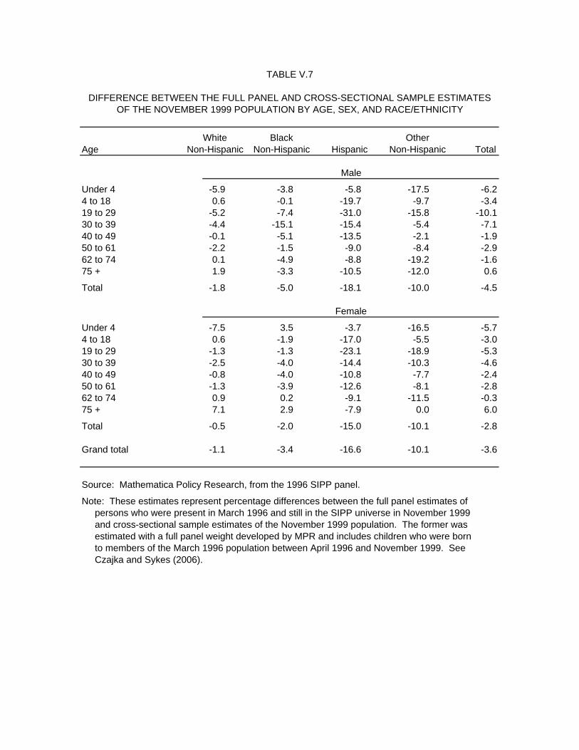
TABLE V.7

DIFFERENCE BETWEEN THE FULL PANEL AND CROSS-SECTIONAL SAMPLE ESTIMATESOF THE NOVEMBER 1999 POPULATION BY AGE, SEX, AND RACE/ETHNICITY

White Black OtherAge Non-Hispanic Non-Hispanic Hispanic Non-Hispanic Total

Male

Under 4 -5.9 -3.8 -5.8 -17.5 -6.24 to 18 0.6 -0.1 -19.7 -9.7 -3.419 to 29 -5.2 -7.4 -31.0 -15.8 -10.130 to 39 -4.4 -15.1 -15.4 -5.4 -7.140 to 49 -0.1 -5.1 -13.5 -2.1 -1.950 to 61 -2.2 -1.5 -9.0 -8.4 -2.962 to 74 0.1 -4.9 -8.8 -19.2 -1.675 + 1.9 -3.3 -10.5 -12.0 0.6

Total -1.8 -5.0 -18.1 -10.0 -4.5

Female

Under 4 -7.5 3.5 -3.7 -16.5 -5.74 to 18 0.6 -1.9 -17.0 -5.5 -3.019 to 29 -1.3 -1.3 -23.1 -18.9 -5.330 to 39 -2.5 -4.0 -14.4 -10.3 -4.640 to 49 -0.8 -4.0 -10.8 -7.7 -2.450 to 61 -1.3 -3.9 -12.6 -8.1 -2.862 to 74 0.9 0.2 -9.1 -11.5 -0.375 + 7.1 2.9 -7.9 0.0 6.0

Total -0.5 -2.0 -15.0 -10.1 -2.8

Grand total -1.1 -3.4 -16.6 -10.1 -3.6

Source: Mathematica Policy Research, from the 1996 SIPP panel.

Note: These estimates represent percentage differences between the full panel estimates of persons who were present in March 1996 and still in the SIPP universe in November 1999 and cross-sectional sample estimates of the November 1999 population. The former was estimated with a full panel weight developed by MPR and includes children who were born to members of the March 1996 population between April 1996 and November 1999. See Czajka and Sykes (2006).

TABLE V.8

DIFFERENCE BETWEEN THE FULL PANEL AND CROSS-SECTIONAL SAMPLE ESTIMATESOF THE SEPTEMBER 2003 POPULATION BY AGE, SEX, AND RACE/ETHNICITY

White Black OtherAge Non-Hispanic Non-Hispanic Hispanic Non-Hispanic Total

Male

Under 4 -2.2 -15.5 -13.6 -0.2 -6.04 to 18 0.4 -2.2 -14.6 -6.7 -3.219 to 29 -8.9 -3.0 -29.5 -14.0 -12.530 to 39 -3.8 -8.2 -19.7 -4.7 -7.240 to 49 -1.7 -7.0 -17.2 -4.6 -4.250 to 61 -2.3 -3.4 -10.8 -5.3 -3.262 to 74 1.2 0.8 -9.9 -6.9 0.175 + 2.8 -4.1 -14.9 -3.6 1.0

Total -2.2 -4.6 -18.3 -6.7 -5.0

Female

Under 4 -6.1 -0.3 6.5 -14.7 -4.04 to 18 0.4 -5.0 -12.4 -8.2 -3.319 to 29 -4.7 -1.9 -16.6 -9.2 -6.530 to 39 -3.2 -2.9 -13.9 -6.0 -5.040 to 49 -1.9 -0.9 -10.3 -4.9 -2.950 to 61 -0.2 -2.9 -11.4 -6.9 -1.762 to 74 -0.1 6.8 -9.4 -9.6 -0.575 + 5.7 -4.1 -7.5 6.7 4.3

Total -1.1 -2.3 -11.9 -7.2 -3.0

Grand total -1.6 -3.4 -15.2 -6.9 -4.0

Source: Mathematica Policy Research, from the 2001 SIPP panel.

Note: These estimates represent percentage differences between the full panel estimates of persons who were present in January 2001 and still in the SIPP universe in September 2003 and cross-sectional sample estimates of the September 2003 population. The former was estimated with a full panel weight developed by MPR and includes children who were born to members of the January 2001 population between February 2001 and September 2003. See Cody et al. (2007).

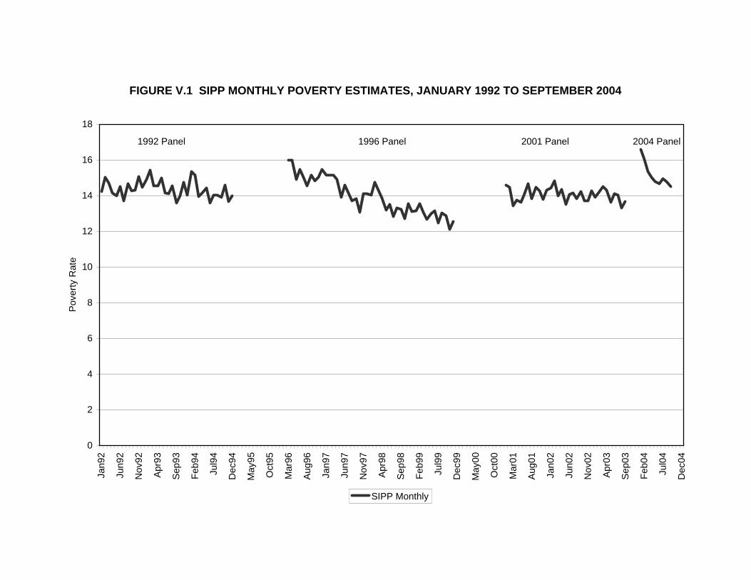
FIGURE V.1 SIPP MONTHLY POVERTY ESTIMATES, JANUARY 1992 TO SEPTEMBER 2004

0

2

4

6

8

10

12

14

16

18

Jan9

2

Jun9

2

Nov

92

Apr

93

Sep

93

Feb

94

Jul9

4

Dec

94

May

95

Oct

95

Mar

96

Aug

96

Jan9

7

Jun9

7

Nov

97

Apr

98

Sep

98

Feb

99

Jul9

9

Dec

99

May

00

Oct

00

Mar

01

Aug

01

Jan0

2

Jun0

2

Nov

02

Apr

03

Sep

03

Feb

04

Jul0

4

Dec

04

Pov

erty

Rat

e

SIPP Monthly

1992 Panel 1996 Panel 2001 Panel 2004 Panel

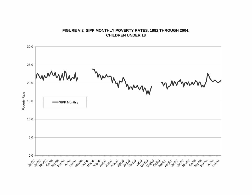
FIGURE V.2 SIPP MONTHLY POVERTY RATES, 1992 THROUGH 2004,CHILDREN UNDER 18

0.0

5.0

10.0

15.0

20.0

25.0

30.0

Jan9

2Ju

n92

Nov92

Apr93

Sep93

Feb94

Jul94

Dec94

May

95Oct9

5M

ar96

Aug96

Jan9

7Ju

n97

Nov97

Apr98

Sep98

Feb99

Jul99

Dec99

May

00Oct0

0M

ar01

Aug01

Jan0

2Ju

n02

Nov02

Apr03

Sep03

Feb04

Jul04

Dec04

Pov

erty

Rat

e

SIPP Monthly

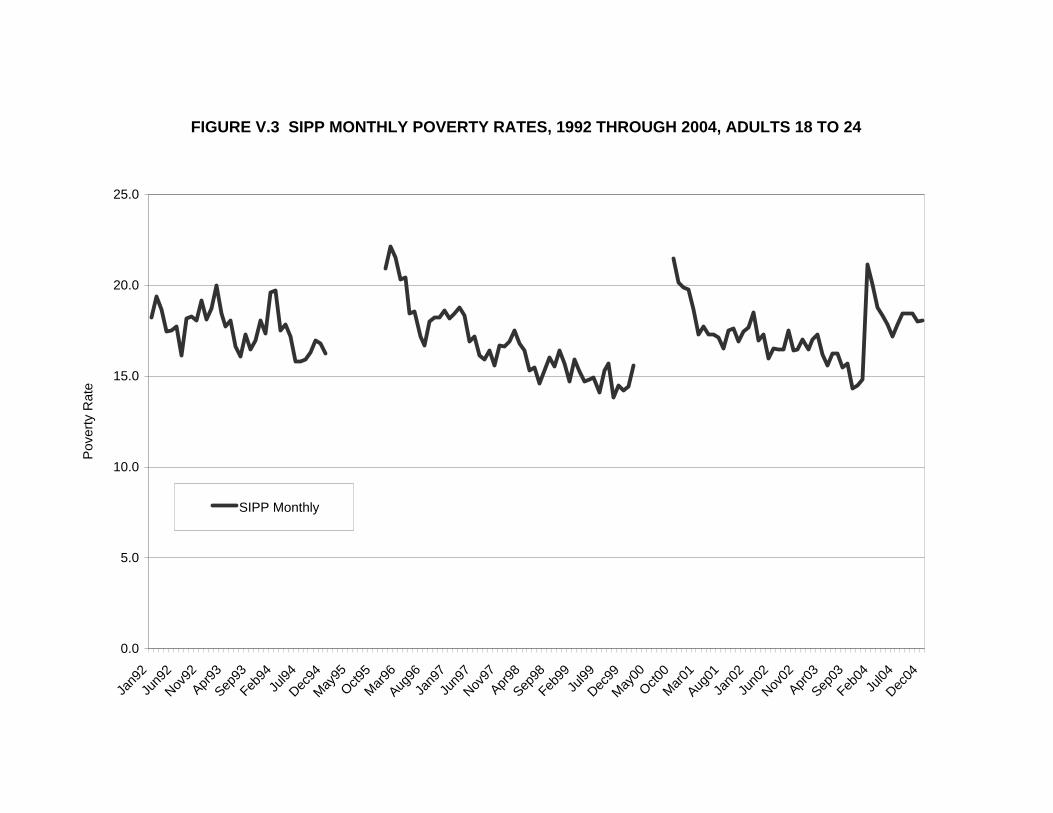
FIGURE V.3 SIPP MONTHLY POVERTY RATES, 1992 THROUGH 2004, ADULTS 18 TO 24

0.0

5.0

10.0

15.0

20.0

25.0

Jan9

2Ju

n92

Nov92

Apr93

Sep93

Feb94

Jul94

Dec94

May

95Oct9

5M

ar96

Aug96

Jan9

7Ju

n97

Nov97

Apr98

Sep98

Feb99

Jul99

Dec99

May

00Oct0

0M

ar01

Aug01

Jan0

2Ju

n02

Nov02

Apr03

Sep03

Feb04

Jul04

Dec04

Pov

erty

Rat

e

SIPP Monthly

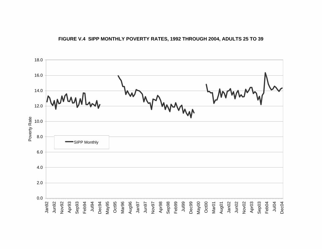
FIGURE V.4 SIPP MONTHLY POVERTY RATES, 1992 THROUGH 2004, ADULTS 25 TO 39

0.0

2.0

4.0

6.0

8.0

10.0

12.0

14.0

16.0

18.0

Jan9

2

Jun9

2

Nov

92

Apr

93

Sep

93

Feb

94

Jul9

4

Dec

94

May

95

Oct

95

Mar

96

Aug

96

Jan9

7

Jun9

7

Nov

97

Apr

98

Sep

98

Feb

99

Jul9

9

Dec

99

May

00

Oct

00

Mar

01

Aug

01

Jan0

2

Jun0

2

Nov

02

Apr

03

Sep

03

Feb

04

Jul0

4

Dec

04

Pov

erty

Rat

e

SIPP Monthly

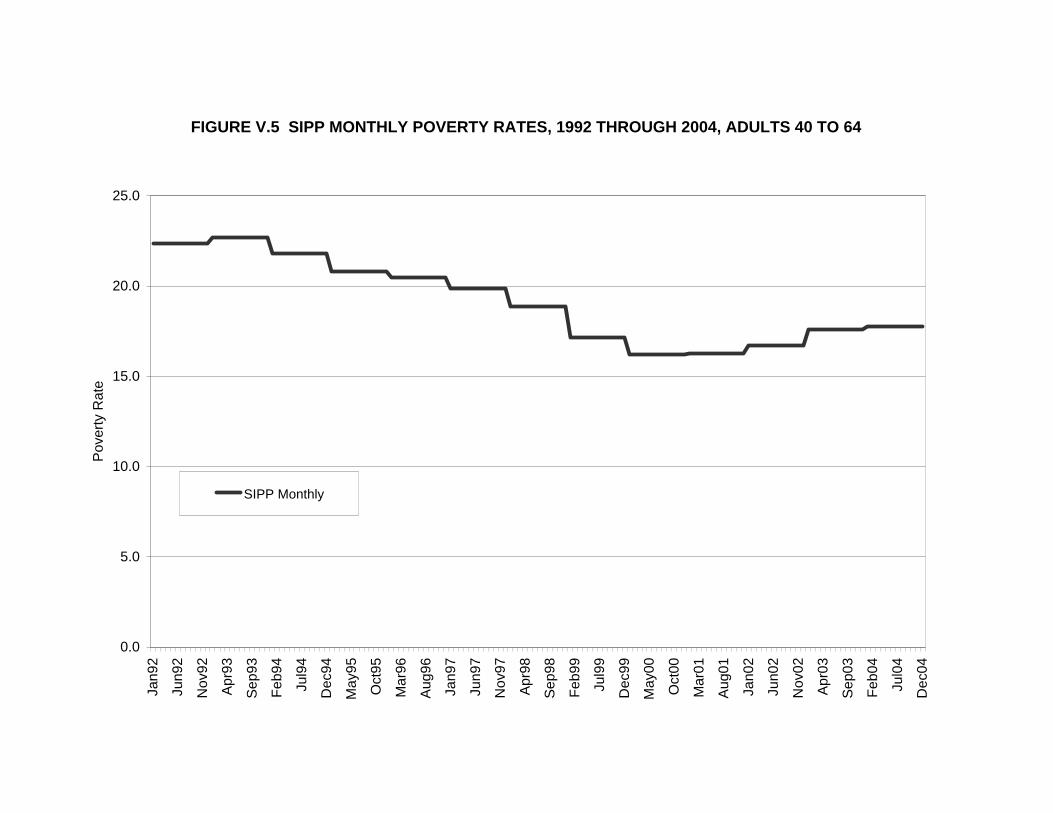
FIGURE V.5 SIPP MONTHLY POVERTY RATES, 1992 THROUGH 2004, ADULTS 40 TO 64

0.0

5.0

10.0

15.0

20.0

25.0

Jan9

2

Jun9

2

Nov

92

Apr

93

Sep

93

Feb

94

Jul9

4

Dec

94

May

95

Oct

95

Mar

96

Aug

96

Jan9

7

Jun9

7

Nov

97

Apr

98

Sep

98

Feb

99

Jul9

9

Dec

99

May

00

Oct

00

Mar

01

Aug

01

Jan0

2

Jun0

2

Nov

02

Apr

03

Sep

03

Feb

04

Jul0

4

Dec

04

Pov

erty

Rat

e

SIPP Monthly

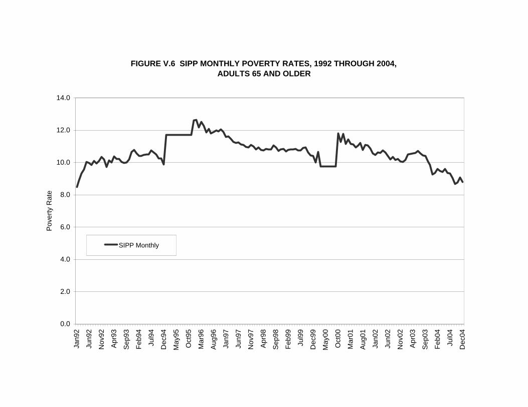
FIGURE V.6 SIPP MONTHLY POVERTY RATES, 1992 THROUGH 2004,ADULTS 65 AND OLDER

0.0

2.0

4.0

6.0

8.0

10.0

12.0

14.0

Jan9

2

Jun9

2

Nov

92

Apr

93

Sep

93

Feb

94

Jul9

4

Dec

94

May

95

Oct

95

Mar

96

Aug

96

Jan9

7

Jun9

7

Nov

97

Apr

98

Sep

98

Feb

99

Jul9

9

Dec

99

May

00

Oct

00

Mar

01

Aug

01

Jan0

2

Jun0

2

Nov

02

Apr

03

Sep

03

Feb

04

Jul0

4

Dec

04

Pov

erty

Rat

e

SIPP Monthly

173

VI. MEASUREMENT OF ECONOMIC WELL-BEING IN THE SIPP AND CPS

In Chapter III we demonstrated that with a detailed demographic calibration, the subsample

of SIPP records that could be matched to SSA administrative records provided an essentially

unbiased representation of the full SIPP sample, whether longitudinal or cross-sectional. In

Chapter IV we presented compelling evidence that, with respect to earnings and both Social

Security and SSI benefit receipt, the SIPP full panel sample can represent an initial population

through time with negligible bias. In Chapter V, however, we found reason to question how well

the SIPP could represent the full cross-sectional population over time—something that the SIPP

was not designed to do but which users have expected it to do. Even if matching bias and panel

attrition do not present the problems that they were believed to present, should SSA be looking

elsewhere to document the changing characteristics of its beneficiary populations over time—

particularly their economic well-being?

Compared to the SIPP, the CPS provides a more fully and consistently representative sample

from year to year, a larger sample size, and more timely and regular release of data. The CPS

captures many of the same types of characteristics that SSA has obtained from the SIPP for

descriptive analyses of its beneficiary populations. Prior to the March 2001 survey, the CPS did

not collect information on the reason for social security benefit receipt, so retired workers,

disabled workers, and other types of beneficiaries could not be differentiated except through

linked administrative records. This deficiency has been addressed with the addition of a question

on the reason for social security benefit receipt. Furthermore, the CPS collects information on

SSI participation that has not been collected in the SIPP, which allows identification of the aged,

blind, and disabled among reported SSI recipients. When the match rate to administrative

records dropped below 60 percent in the SIPP 2001 panel, the CPS was matching 70 percent of

174

adults and 90 percent of children under 15 (Chapter II). The match rate in both surveys is

expected to rise to about 90 percent with the introduction of new methods of matching survey

records to administrative records in 2006.

For ORES analysts who are accustomed to working with the SIPP, the principal issue with

the CPS remains the quality of its income data relative to what is collected in the SIPP. Building

on what we presented in the preceding chapter, this chapter focuses on the comparative strengths

of the two surveys in describing the economic well-being of the population in general and elderly

and lower-income persons in particular. In Section A we compare the two surveys with respect

to their identification of sources of income, including their estimation of Social Security

beneficiaries’ reliance upon their Social Security benefits as a principal source of income. In

Section B we turn from sources of income to amounts, comparing the two surveys in their

capture of total income and its major components. In Section C we look at the measurement of

income in relation to the poverty threshold, comparing the two surveys’ estimates of poverty

rates over time. Finally, in Section D we summarize our principal findings and conclusions.

A. SOURCES OF INCOME

Dating back to the first SIPP panel, one of the recognized strengths of the survey has been

its identification of more sources of income than other surveys. Using SIPP and CPS data from

the 1990s and early 2000s, we compare the two surveys with respect to (1) their estimates of

Social Security beneficiaries’ reliance upon Social Security benefits as their principal source of

income and (2) their identification of combinations of income sources across the population.

1. Reliance upon Social Security Benefits

One of the applications of SIPP data identified by SSA involves estimates of Social Security

beneficiaries’ reliance upon Social Security as a principal source of income. The proportion of

personal or family income derived from social security benefits can be estimated with both the

175

CPS and the SIPP and, therefore, provides a good basis for assessing whether CPS data can be

substituted for SIPP data to address a question of interest to researchers and policymakers at

SSA.

SIPP and CPS estimates of Social Security payments as a percentage of total personal

income among retired workers in calendar year 2001 are compared in Table VI.1. While there

are similarities in the estimates, the differences are more striking. Most notably, the CPS shows

that social security payments accounted for 100 percent of the total personal income of 22

percent of retired workers whereas the SIPP shows less than 8 percent of retired workers having

no income besides their social security payments. Roughly these same percentages are found for

retired workers at ages under 65, 65 to 74, and 75 and older. If the SIPP shows substantially

fewer retired workers receiving all of their reported personal income from Social Security

payments, then the SIPP must show relatively more retired workers receiving smaller fractions

of their income from Social Security payments. For retired workers under 65 the biggest

difference occurs in the proportion receiving less than 25 percent of their income from Social

Security payments. The SIPP finds 30 percent of retired workers receiving less than 25 percent

of their income from Social Security payments compared to 18 percent for the CPS.

Furthermore, since retired workers under 65 are not yet covered by Medicare, the fact that the

2001 SIPP panel collected net rather than gross Social Security benefits would not have

contributed to the lower Social Security benefit share in the SIPP than the CPS. Among older

retired workers, for whom the collection of net versus gross benefits in the SIPP was almost

certainly a factor, there was no difference between the SIPP and the CPS in the proportion

reporting Social Security payments less than 25 percent of their total personal income. Instead,

the difference between the two surveys occurred in the proportion reporting benefits that were

between 25 and 75 percent of their total personal income.

176

These patterns are repeated at the family level, where we measure the Social Security

benefits received by each retired worker’s family as a proportion of total family income (Table

VI.2). Expanding the unit of analysis to the family reduces the relative importance of Social

Security benefits because the incomes of non-beneficiaries are included with those of retired

workers in some cases. Nevertheless, striking differences between the CPS and SIPP remain.

Fewer than 4 percent of retired workers in the SIPP compared to 13 percent in the CPS reported

no other family income in 2001 besides what they received in Social Security payments. As with

personal income, these proportions varied little by the age of the worker. Here, too, retired

workers under 65 in the SIPP were more likely than those in the CPS to report less than 25

percent of their family income as coming from Social Security payments: 43 percent versus 31

percent. Among older retired workers the difference between the SIPP and the CPS was

concentrated among those receiving between 25 and 75 percent of their income from Social

Security payments.

We tabulated both surveys to determine what accounted for the SIPP’s smaller proportion of

Social Security beneficiaries with no other sources of income. Results for family income are

reported in Table VI.3. Retired workers in the SIPP were more likely than their counterparts in

the CPS to report receiving each of the six additional sources that we examined: wages, self-

employment, property income, pensions, SSI, and welfare.1 Differences in the receipt of

wages—13 percentage points among workers under 65—were small after age 65, but large

differences in the receipt of property income and especially pensions were evident at all ages.

1 Because we wanted to look at combinations of sources, we excluded a number of other transfers that

accounted for very small percentages of retired workers’ family income. These included unemployment compensation, worker’s compensation, veterans’ payments, Black Lung, disability compensation, and other government income as well as child support, alimony, charity, casual earnings, miscellaneous cash income, and income from friends and roomers.

177

In addition to being less likely to report that their only source of family income was Social

Security, retired workers at all ages in the SIPP were less likely than those in the CPS to report

only one additional source of income. Retired workers under age 65 were equally likely in both

surveys to report two additional sources, but those in the SIPP were more likely to report exactly

three additional sources (33 percent versus 20 percent) or four or more additional sources (8

percent versus 2 percent).

The number of additional sources declines with age—largely because of workers

withdrawing from the workforce. In the SIPP, the reduction in sources is seen in the proportion

with three or more, which declines from 41 percent to 18 percent, producing a substantial

increase in the proportion of retired workers with exactly two sources (from 38 to 54 percent) but

only small increases in the proportion with no additional sources or only one additional source.

In the CPS the reduction in the proportion of retired workers with three or more additional

sources of income (from 22 percent to 8 percent) has little effect on the proportion with exactly

two additional sources, which changes from 39 percent to 37 percent. Instead, the effect is seen

on the proportion with even fewer sources. While the proportion of SIPP retired workers with

only one additional source grows by only 5 percentage points (from 18 to 23 percent) with the

worker’s age, this same proportion in the CPS grows by 12 percentage points (from 26 to 38

percent).

The broad receipt of property income and pensions—the two most common additional

sources among retired workers at all ages in both surveys—is evident in their prominence in the

modal combinations of additional sources. Property income and pensions is the modal

combination of two additional sources in both surveys at all ages, followed by wages and

property income. The latter combination diminishes with age while the former combination

grows. Wages, property income and pensions is the modal combination of three additional

178

sources, with no other combination being close. In the SIPP but not the CPS, retired workers at

every age are much more likely to have this combination of three sources than just wages and

property income alone. In the CPS somewhat more retired workers under age 65 have all three

sources than just wages and property income, but among older workers the proportions having

all three versus just the two are the same.

These findings raise serious concerns about using the CPS to examine issues related to

reliance on Social Security income and, more generally, the sources of financial support among

retired workers. The SIPP’s greater effectiveness in capturing income from multiple sources

among Social Security retired workers supports the ORES analysts’ preference for the SIPP over

the CPS and demonstrates an important way in which the SIPP appears to provide a better

vehicle for policy analysis.

2. Sources of Income among All Persons by Age

The SIPP’s superiority in capturing sources of income extends beyond retired workers to

persons of all ages although both surveys report the same frequency of wage and salary

income—even among the elderly. Tables VI.4 through VI.7 compare CPS and SIPP estimates of

the distribution of persons by sources of family income at three points in time—1992, 1997, and

2001. Each table presents estimates for one of four age groups: 65 and older, 40 to 64, 18 to 39,

and under 19.

Among the elderly, the SIPP obtains slightly higher reports of Social Security and SSI

recipiency, with the difference between the two surveys growing over time (Table VI.4).

Between 1992 and 2001 the difference in the estimates of Social Security receipt grew from 1

percentage point to nearly 5 percentage points. For SSI the gap widened from 1 percentage point

in 1992 to nearly 4 percentage points in 1997 as SSI reporting declined in the CPS but rose in the

SIPP. The pattern for these two sources was repeated for self-employment and, with much lower

179

rates of receipt, welfare. The biggest difference between the two surveys lies in their capture of

property income and pensions. For property income, an 11 percentage point difference in 1992

grew to 16 percentage points in 2001. For pensions, the CPS shows reported recipiency

declining from 49 percent to 44 percent between 1992 and 2001 while the SIPP shows a 16

percentage point increase, from 56 percent to 70 percent.

There is only a small difference between the SIPP and CPS in the proportion of elderly

persons with no reported sources of income. Much bigger differences exist in the percentage

reporting multiple sources. In 1992, only 0.2 percent of elderly persons in the CPS and 0.1

percent in the SIPP had no reported family income. The SIPP percentage did not change over

time while the percentage in the CPS rose, slightly, to just under 1 percent. Elderly persons in

the CPS were more likely to have only one or two reported sources of family income and less

likely to have three or more. Over time, the CPS showed an increase in the proportion reporting

only one source of income (from 12 to 17 percent versus a consistent 6 percent in the SIPP) and

a reduction in the proportions reporting three or more sources (from 55 percent to 47 percent).

The SIPP, by contrast, showed between 48 and 50 percent reporting exactly three sources of

income, with an increase in the proportion reporting four our more sources (from 17 to 24

percent) and a reduction in the proportion reporting only two sources of income (from 28 to 20

percent). The modal combination of sources—Social Security, property income and pensions—

declined from 28 percent to 22 percent in the CPS while rising from 36 percent to 38 percent in

the SIPP.

That the SIPP improved relative to the CPS could be attributable to design changes in both

surveys, with both transitioning to computer-assisted interviewing (in survey year 1994 for the

CPS and 1996 for the SIPP) but the SIPP receiving a more substantial revision of its instrument.

180

These design changes will be revisited in the next section of this chapter when we look at

aggregate income.

Among adults 40 to 64, the reported frequency of wages held at 86 to 87 percent in the CPS

while rising from 85 to 87 percent in the SIPP (Table VI.5). Self-employment declined from 16

to 13 percent in the CPS while holding steady at 22 percent in the SIPP, such that the frequency

of either wage or self-employment earnings ran 1 to 2 percentage points higher in the SIPP than

the CPS. The reported receipt of property income declined by 5 percentage points in both

surveys, remaining 11 to 12 percentage points higher in the SIPP (75 versus 63 percent in 2001).

Reported recipiency declined for all four of the remaining sources in the CPS but rose for three

of these in the SIPP, so that what was initially a very small gap between the two surveys in 1992

grew in each case. Pensions showed the strongest relative gain for the SIPP, with recipiency in

the CPS falling from 15 to 12 percent while rising from 17 to 21 percent in the SIPP. Social

Security and SSI were reported very slightly more often in the SIPP than the CPS in 1992, but

Social Security recipiency declined by a percentage point in the CPS while rising by that same

amount in the SIPP. SSI remained steady in the CPS but rose by 2 percentage points in the SIPP.

Lastly, welfare recipiency declined by 2 percentage points in both surveys with the SIPP

remaining a percentage point higher than the CPS.

The proportion of adults 40 to 64 with no reported sources of family income reached 1.5

percent in the CPS while remaining at 0.5 percent in the SIPP. Around half of the persons in

each survey had exactly two sources of family income, but the SIPP respondents were more

likely to report three or more sources and less likely to report only one source. CPS respondents

became less likely to report multiple sources over time, with the proportion reporting only one

source rising from 20 percent to 26 percent. In the SIPP this proportion rose as well, but by only

2 percentage points, from 12 to 14 percent. In both surveys about 40 percent reported receiving

181

both wages and property income, which was the modal combination. Only in the CPS did any

other combination of sources account for even half that frequency; the proportion of CPS

respondents reporting only wages rose from 16 to 21 percent. SIPP respondents were as likely to

report wages in combination with property income and self-employment as to report only

wages—around 11 percent in each case in 2001.

Among younger adults, 18 to 39, the percentage reporting family wage income rose by a

percentage point in both surveys, with the SIPP remaining a percentage point ahead of the CPS,

but self-employment declined from 12 to 10 percent in the CPS while remaining at 17 percent in

the SIPP. The frequency of any earnings approached 98 percent in the SIPP versus 95 percent in

the CPS. Property income was reported less often than among older adults in both surveys, but

the SIPP maintained a 15 to 16 percentage point edge, with 68 percent of SIPP respondents in

2001 reporting family incomes that included this source compared to 52 percent in the CPS.

While the levels were small, pension receipt declined by 2 percentage points (to 3 percent) in the

CPS while rising by a percentage point (to 8 percent) in the SIPP. Social Security receipt

declined by a percentage point to 7 percent in the CPS while remaining at 10 percent in the SIPP

whereas SSI recipiency was stable at 3 percent in the CPS but rose from 4 to 6 percent in the

SIPP. Welfare recipiency declined by 4 percentage points in both surveys but was twice as high

in the SIPP as in the CPS in 2001 (4.6 versus 2.3 percent).

With respect to the number of reported sources, the principal difference between the two

surveys was in the reporting of multiple versus a single source of income. In the CPS the

proportion of persons with no reported source of income grew from 1.5 to 2.4 percent compared

to an average of 0.6 percent in the SIPP. The proportion reporting only one source of income

rose in both surveys, as it did with adults 40 to 64, but the initial level was higher and the

increase more substantial in the CPS than the SIPP. The proportion with only one source rose

182

from 30 to 38 percent in the CPS versus 17 to 22 percent in the SIPP. The proportion with

exactly two sources declined by an offsetting amount in the SIPP (from 58 to 54 percent), such

that the proportion reporting three or more sources did not change, remaining at 24 percent. In

the CPS the proportion reporting exactly two sources declined by 4 percentage points as well

(from 52 to 48 percent), but with the larger increase in the proportion reporting only one or no

sources of income the proportion reporting three or more sources declined from 16 percent to 11

percent.

As with persons 40 to 64, the modal combination of sources was wages and property

income, which accounted for between 41 and 43 percent of the CPS respondents and 46 to 49

percent of the SIPP respondents. Persons with wages as their only reported source of family

income rose from 27 to 35 percent in the CPS and from 14 to 20 percent in the SIPP. The only

other significant combination or single source in either survey was wages, property income and

self-employment, held by 5 percent of CPS respondents, on average, and 10 percent of SIPP

respondents.

Reported sources of family income among children differ only marginally from the reported

sources among the families of adults 18 to 39, which include most of their parents. Children’s

families show higher receipt of welfare and self-employment along with lower receipt of wages

and property income—all of these differentials stronger in 1992 than 2001—but similar levels of

Social Security, pensions, and SSI. In all three years the SIPP showed a higher incidence of

every reported source of income than the CPS, although the difference for wages was less than a

percentage point (but very consistent across years). In addition, the SIPP was more likely to find

multiple sources of income. While 38 percent of children’s families in the CPS had only one

source or no source of income in 2001, the corresponding figure for the SIPP was only 22

percent. In that same year 26 percent of children’s families in the SIPP had three or more

183

reported sources of income compared to just 11 percent in the CPS. The corresponding figures

in 1992 were 25 percent for the SIPP and 16 percent in the CPS, so we again see a relative

improvement for the SIPP.

On the whole then, this analysis indicates that across all age groups—but particularly

children and the elderly—the SIPP has continued to identify more sources of family income than

the CPS. Furthermore, the SIPP’s evident superiority in this regard has grown since 1992,

although a fall-off in the identification of sources in the CPS appears to have played a bigger role

in broadening this differential than the recorded gains in the SIPP.

If the SIPP has continued to identify more sources of income than the CPS, has the SIPP

also captured more income than the CPS? We turn next to estimates of aggregate income to

address this question.

B. AGGREGATE INCOME

When the SIPP was new, comparisons of SIPP and CPS estimates of aggregate income—

often in relation to independent benchmarks—established the comparative strengths of the two

surveys with respect to the measurement of income. In one detailed assessment, the SIPP’s

aggregate estimate of regular money income (that is, income excluding certain lump sums) was

99.9 percent of the corresponding CPS aggregate, with the SIPP running about 5 percent lower

on wages and salaries (nearly three-quarters of total CPS income) but substantially higher on

virtually everything else (Vaughan 1993). The SIPP’s superiority—both actual and potential—

as a vehicle for the measurement of economic well-being was recognized in the recommendation

of a National Academy of Sciences panel that the SIPP replace the CPS as the source of official

poverty statistics in the U.S.

The work of Vaughan and others was updated by Roemer (2000), who compared estimates

of aggregate income from the SIPP and CPS with independent benchmarks derived from

184

National Income and Product Accounts (NIPA) data over the period from 1990 to 1996. In the

first subsection below we present comparative estimates of aggregate income derived from

Roemer’s work. Following that we extend the comparison to quintiles based on total income in

order to compare the surveys’ estimates of income by source at different parts of the income

distribution. Lastly we examine trends in the proportion of aggregate income that is imputed in

the two surveys. This, too, is presented by quintile of total income.

1. Comparative Estimates of Aggregate Income

By 1990, the SIPP estimate of total income had slipped below 98 percent of the CPS

aggregate, and it fell further behind over the first half of the decade, ending at 92.5 percent of the

CPS aggregate in 1996, the first year of the SIPP redesign (Table VI.8). Over this period the

SIPP estimate of wage and salary income declined from 94 percent to 89 percent of the CPS

estimate, matching the overall decline. But the SIPP fell most in its capture of property income.

Excluding the two years when spikes in the SIPP estimates of dividends pushed the survey’s

estimate of total property income above the CPS, the SIPP aggregate dropped from 95 percent to

81 percent of the CPS aggregate. While the SIPP estimate of rent and royalties remained well

above the CPS estimate throughout the period, SIPP dividend income eventually dropped below

CPS dividend income while SIPP interest income, which started out below the CPS, fell further

behind, going from 84 percent to just 60 percent of the CPS amount. SIPP estimates of transfer

income also declined relative to the CPS, dropping from 105 percent to 98 percent of the CPS

total. Only pension income as a class improved in the SIPP, growing from 95 percent of the CPS

aggregate to 112 percent on the strength of gains in the capture of private pensions and military

retirement income, although the 1996 estimate of the latter is clearly an outlier.

Did the CPS get better over this period, or did the SIPP get worse? Roemer’s estimates of

SIPP and CPS aggregates as a percentage of the NIPA benchmarks indicate that the answer

185

varies by source. Over all sources, SIPP aggregate income declined by 1 to 2 percentage points

relative to the NIPA benchmark while the CPS improved by about 3 percentage points (Tables

VI.9 and VI.10). For wage and salary income, SIPP declined by 2 percentage points relative to

the benchmark between 1990 and 1995 but then rose by 3 percentage points between 1995 and

1996, for a net gain of 1 percentage point. The CPS estimate of wage and salary income rose by

6 percentage points over the entire period, with most of the increase occurring between 1992 and

1993, when the computer-assisted instrument was introduced. The SIPP increase also coincided

with the introduction of computer-assisted interviewing in 1996.

Other sources of income present a mixed picture. Estimates of self-employment income

declined substantially in relation to the NIPA benchmark in both surveys. Estimates of total

property income declined by about 9 percentage points in the SIPP while increasing by 7 to 10

percentage points in the CPS. Estimates of all three component sources of property income

declined in the SIPP, as did the CPS estimates of rent and royalties, but estimates of interest and

dividends improved markedly in the CPS.

Transfer income in the SIPP fell by about 6 percentage points relative to the benchmark

while holding steady in the CPS. Among the individual sources of transfer income, SIPP

estimates of Social Security and Railroad Retirement, unemployment compensation, and

veterans’ payments deteriorated over the period. Estimates of worker’s compensation declined

substantially between 1990 and 1995 but showed a 20 percentage point rise between 1995 and

1996. SSI and other cash welfare also exhibited sharp increases between 1995 and 1996, but it

remains to be seen if these gains will persist. The CPS estimates of worker’s compensation fell

off substantially over the period while veterans’ payments improved. Most of the other sources

were stable while other cash welfare rose to the level of the benchmark in 1993 through 1995 but

then dropped below the 1990 level.

186

Lastly, pension estimates improved by a percentage point in the SIPP while declining by 12

percentage points in the CPS. Estimates of private pensions improved in the SIPP but fell off

slightly in the CPS. Estimates of military retirement declined substantially in the CPS while

holding steady in the SIPP until a 16 point increase between 1995 and 1996. State and local

employee pensions showed a steady decline in the CPS while holding steady in the SIPP until a

modest decline between 1995 and 1996.

On the whole, the transition to a computer-based instrument appears to have been more

beneficial to the CPS than the SIPP. The CPS estimate of total income improved by nearly 4

percentage points relative to the benchmark in the year that computer-assisted interviewing was

introduced (reference year 1993) and remained slightly above that level for the next three years.

The SIPP estimate of total income improved by a percentage point when computer-assisted

interviewing was introduced in 1996, but Roemer’s data end in that year, so we cannot tell if the

SIPP maintained that level of coverage relative to the benchmark.

2. Income by Quintile

While the CPS may have moved past the SIPP in its capture of aggregate income, despite

finding lower levels of recipiency for most sources, estimates of aggregate income for many

sources are affected disproportionately by respondents in the upper tail of the distribution, where

the CPS appears to be much more successful than the SIPP (Roemer 2002; Czajka et al. 2003).

For SSA’s purposes, the SIPP’s performance lower in the income distribution is far more

important.

To examine how the SIPP and CPS compared in their estimates of aggregate income at

different parts of the income distribution, we divided each sample into quintiles based on total

187

family income and performed comparisons within each quintile.2 Benchmarks cannot be

constructed for such purposes because the required data do not exist. We were limited, then, to

comparing estimates between the two surveys, which we did at three points in time: 1993, 1997,

and 2002. The SIPP estimates are from the 1992, 1996, and 2001 panels and, for consistency,

are derived from the second year of data in each panel.3 The CPS estimates are from the 1994,

1998, and 2003 supplements, so all three reflect the computer-assisted instrument.

Our estimates are based on public use data rather than the Census Bureau’s internal files, so

amounts are topcoded. This affects the SIPP estimates more than the CPS because of the way

that topcodes are assigned in the two surveys. In the CPS, the topcodes that appear on the public

use file are the means of the values that were replaced by topcodes, so that the sum of the

topcoded values equals the sum of the values on the Census Bureau’s internal file—that is, prior

to topcoding.4 In the SIPP, all topcoded amounts are simply truncated; thus the sum of topcoded

amounts understates the sum of the corresponding reported amounts. In addition, our estimates

from both surveys exclude the families of armed forces personnel, which should not favor either

survey, but they also include certain lump sum pension payments, which tends to favor the SIPP.

Finally, we used the 1992 SIPP panel for the 1993 estimates whereas Roemer used the 1993

panel. Despite these differences, our estimates line up reasonably well with Roemer’s estimates

for 1993. While there are differences by source, our estimate of SIPP aggregate income as a

2 More specifically, we classified people by their family income and assigned the bottom 20 percent of persons

to the first quintile, the next 20 percent to the second quintile, and so on.

3 As noted previously, the 1996 panel started two months late and did not collect data for all 12 months of 1996 for two of the four rotation groups.

4 For earnings, separate means are calculated for 12 subpopulations defined by combinations of sex, race and Hispanic origin, and work experience so that users can reproduce the internal file means and totals for these important subgroups (U.S. Census Bureau 2003).

188

percentage of CPS aggregate income, at 94.5, compares quite closely to Roemer’s estimate of

94.8.

While the ratio of SIPP to CPS total income declined from 94.5 percent to 89.0 percent

between 1993 and 1997, there was no further decline between 1997 and 2002 (Table VI.11).

SIPP wages and salaries declined from 84.6 percent to 82.4 percent of the CPS aggregate, but

this was offset by small improvements in every other source. If we exclude the top quintile so as

to eliminate the impact of topcoding and the CPS’s more effective capture of very high incomes,

mentioned earlier, we find that the SIPP does indeed reach a higher fraction of the overall CPS

aggregate: 98.2 percent in 1993 versus 94.5 percent when all five quintiles are included (Table

VI.12). Furthermore, the decline between 1993 and 1997 is smaller at 2.9 versus 5.5 percentage

points. However, the SIPP estimate declines another percentage point, relative to the CPS,

between 1997 and 2002.

Besides wages and salaries, three other sources show small declines in SIPP coverage

between 1997 and 2002: property income, Social Security, and welfare. In both tables, though,

the ratios of SIPP to CPS aggregates are generally quite similar between 1997 and 2002,

suggesting some stabilization in the relative performance of the two surveys after the CPS’s

earlier gains.

Turning to the results by income quintile, we begin with the lowest quintile, where the SIPP

has historically performed best in relation to the CPS. The conventional wisdom is that the

combination of thrice-yearly interviews and the SIPP’s collection of data for individual calendar

months is more effective than the CPS’s annual interviews in capturing irregular income flows,

which are more characteristic of the lower end of the income distribution than the rest of the

distribution. In 1993 the SIPP captured 20 percent more income from the lowest quintile than

the CPS, including 25 percent more wages and salaries, 157 percent more self-employment

189

income (due in part to differences in how self-employment income is defined in the two

surveys), 22 percent more property income, 7 percent more Social Security and Railroad

Retirement, 12 percent more SSI, 24 percent more other transfers, and 44 percent more pension

income (Table VI.13). Between 1993 and 1997, however, the SIPP’s edge in total income

dropped to 12 percentage points, and by 2002 it had fallen to just 6 percentage points.

With the exception of property income, welfare and other transfers, SIPP aggregates grew at

a brisk rate between 1993 and 1997 and continued to show strong growth between 1997 and

2002, but the CPS aggregates grew even more rapidly. Only for SSI, welfare, and pensions did

the SIPP hold steady or improve relative to the CPS between 1993 and 2002. The SIPP’s

estimate of aggregate wages and salaries, still the largest source of income in the lowest quintile

but not nearly as dominant as at higher income levels, dropped from 125 percent of the CPS

aggregate to 109 percent. Social Security and Railroad Retirement, the second largest source,

dropped from 107 percent of the CPS aggregate to only 88 percent.

In the second income quintile, the SIPP captured 1.5 percent more aggregate income than

the CPS in 1993, but this dropped to 96 percent by 1997 (Table VI.14). Unlike the first quintile,

however, the SIPP held ground after that, gaining back a percentage point by 2002. The SIPP

estimate of wages and salaries dropped from 100 percent of the CPS amount to 92 percent in

1997 but rose to 94 percent in 2002. Property income fell from 112 percent to 90 percent of the

CPS amount while Social Security and Railroad Retirement fell from 97 percent to 90 percent.

Other transfers dropped from 90 percent to 59 percent of the CPS amount. Sizable

improvements relative to the CPS were recorded for self-employment, SSI, welfare, and

pensions, however.

These basic patterns were repeated in the third and fourth quintiles, where the SIPP

estimates of aggregate income fell by 2 to 3 percentage points relative to the CPS, ending up at

190

93 percent in the third quintile and 91 percent in the fourth quintile (Tables VI.15 and VI.16).

There was one notable exception to the patterns by income source; the capture of Social Security

and Railroad Retirement in the SIPP improved between 1997 and 2002 to the point where SIPP

captured relatively more of such income in comparison to the CPS in 2002 than in 1993. In both

cases, the SIPP aggregates in 2002 exceeded the CPS aggregates. Elsewhere, SIPP fell further

behind the CPS in wages and salaries, property income and other transfers but improved in self-

employment, SSI, welfare, and pensions. In both quintiles, SIPP captured 50 percent more

pension income in 2002 than did the CPS.

In the top quintile the SIPP’s estimate of aggregate Social Security and Railroad Retirement

dropped relative to the CPS, as it did in the first and second quintiles, and the relative gain in the

capture of pension income was more modest than in the lower quintiles (Table VI.17).

Otherwise, the different sources improved or declined in the SIPP just as they did in the lower

quintiles. Over all sources, the SIPP estimate of total income in the top quintile dropped from 89

percent of the CPS estimate in 1993 to 81 percent in 1997 but then rose to 83 percent in 2002.

3. Proportion of Income That Is Imputed

Item nonresponse is higher on income questions than on most other types of questions.5

Missing amounts are imputed in both the SIPP and the CPS. The proportion of income that is

imputed is a particularly good statistic for comparing the impact of nonresponse to income items

on estimates of income across surveys. This measure gives greater weight to nonresponse on

items and individual records that account for larger shares of total income. Item nonresponse

rates are less effective for this purpose because the number of questions included in the income

5 Item nonresponse on asset questions is even higher.

191

battery varies substantially across surveys, and the likelihood of nonresponse to one or more

questions increases with the number of questions.6

Two sets of SIPP estimates are presented in Table VI.18—one covering the four years 1992,

1993, 1997 and 2002 and the other two covering only the final two years. When an amount field

in the SIPP is missing because of nonresponse to an earlier recipiency question, the allocation

flag that is associated with the amount field may not identify the amount as imputed. For some

amount fields it is necessary to work backwards through a complex chain of allocation flags to

fully identify the imputed values. We did this for 1997 and 2002, but 1992 and 1993 presented

complications because of instrument changes and a complete renaming of variables that attended

the 1996 redesign. Consequently, we did not identify all of the imputed amounts in 1992 and

1993. Instead we replicated this more limited identification of imputed amounts on the 1997 and

2002 data, which gave us a consistent time series and a way of gauging how much imputed

income we may have missed in 1992 and 1993.

The first set of SIPP estimates in Table VI.18 uses the more limited method of identifying

imputed amounts in all four years. The second set reflects a full identification of imputed

amounts in 1997 and 2002, which adds only 0.7 percentage points to the income imputation rate

in 1997 and 0.4 percentage points in 2002. For four of the income sources the two sets of

estimates are identical, and for two others they differ by only 0.2 to 0.3 percentage points. The

differences between the two sets of estimates are somewhat larger for SSI (0.5 and 1.2

percentage points) but they are substantially larger for property income, which has the highest

imputation rate by either measure and is estimated from a complex sequence of questions that

give respondents a lot of difficulty, apparently. For all of the sources except property income,

6 Because of this, the proportion of respondents with any income items imputed is a particularly weak measure

for comparative purposes

192

then, the trend in the version 1 estimates is either identical to or very similar to the trend that we

would see with full identification of imputed income for all four years. For property income the

large differences between the version 1 and version 2 estimates in 1997 and 2002 create

substantial uncertainty about the full level of income imputation in the earlier years.

Table VI.18 presents two sets of CPS estimates as well, but each set covers all four years.

The two sets differ in whether or not they include the income imputed to persons who responded

to the monthly labor force survey but did not complete the supplement. When we exclude the

whole person imputes from both the numerator and denominator, as we do in the middle panel of

Table VI.18, the estimated proportion of income imputed reflects only item nonresponse to the

income questions among the respondents to the supplement. If we want to assess the

comparative impact of imputation for item nonresponse in the SIPP and CPS, then this is the

most appropriate statistic with which to do so. If, on the other hand, our goal is to evaluate the

total impact of income imputation in the two surveys, then it is important to include the income

imputed to nonrespondents to the supplement, which we do in the bottom panel of Table VI.18.7

Since all of the income for this segment of the CPS sample is imputed, these whole person

imputations account for a substantial but largely fixed share of total income in the CPS. In 2002

the income imputed to this segment represented 10.7 percent of total CPS income, which is

comparable to its share of the weighted sample.8, 9

7 The relationship between the two statistics is as follows. To calculate the imputation rate with whole person

imputes included, we add the amount of income imputed to these respondents to both the numerator and denominator of the imputation rate without whole person imputes.

8 Note that this is not the difference between the 34.2 percent imputation rate when whole person imputes are included and the 26.3 percent imputation rate when they are not included. The latter figure was calculated over a denominator that excluded the income due to whole person imputes. We must include this imputed income in the denominator in order to determine the share of total CPS income that is due to imputation for item nonresponse. This fraction was 23.5 percent in 2002.

9 Nonrespondents to the supplement accounted for 10.0 percent of the weighted CPS sample in March 2002; we do not have a figure for the March 2003 sample.

193

In the SIPP’s initial year, the proportion of aggregate income that was imputed was just over

half the percentage imputed in the CPS—11.4 percent of aggregate regular money income for the

SIPP compared to 20.1 percent in the CPS (Vaughan 1993).10 From the tabulations presented in

Table VI.18 it is apparent that imputation grew more rapidly in the SIPP than in the CPS over the

next few years. By 1992, imputed income accounted for about 18 percent of total income in the

SIPP versus 23 percent in the CPS (with whole person imputations included). Income

imputation in both surveys grew substantially over the next 10 years, rising to 29 percent of total

income in the SIPP and 34 percent in the CPS, but the difference between the two surveys

remained at 5 percentage points.

When whole person imputes are excluded from the CPS numbers, we find that the income

imputation rates in the SIPP were higher for every source of income in 1992, with a 5 percentage

point difference for total income. For every income source, then, item nonresponse was a bigger

problem in the SIPP than in the CPS, and this was true even with the incomplete identification of

all the imputed income for some of the SIPP sources.

Between 1992 and 1993 the SIPP imputation rates rose for every income source, with a 3

percentage point increase overall. The fact that the estimates for the two years are from the same

panel might suggest that the increase is a panel phenomenon.11 However, the CPS shows a

similar increase without the whole person imputes. When the whole person imputations are

included, the CPS shows less than a percentage point increase between the two years.

Apparently, nonresponse to the income items rose between 1992 and 1993, but unit nonresponse

to the supplement declined. This latter is noteworthy because 1993 represents the first year of

10 Judging from its magnitude, the CPS figure includes income allocated as a result of whole person

imputations (about 8 percent of supplement sample households, unweighted; see Table II.4).

11 This could be explored with the 2001 panel, but we have not done so.

194

computer-assisted interviewing in the CPS. Some have speculated that with computer-assisted

interviewing the transition from the labor force questionnaire to the supplement became almost

seamless, giving respondents less opportunity to refuse the supplement. Any such impact was

not long lasting, however. Between 1997 and 2002, the CPS shows about the same increase in

its income imputation rate whether or not the whole person imputes are included.

Between 1993 and 2002, the proportion of total income that was imputed increased by 8

percentage points in the SIPP and by 10 to 11 percentage points in the CPS, depending on

whether whole person imputes were included or not. In the CPS, the imputation rates for all but

two sources increased by about the same amount. The exceptions were property income, for

which the imputation rate increased by 23 percentage points, and SSI, for which the increase was

only 4 percentage points. For property income the increased raised the imputation rate to 58

percent without the whole person imputes.

For the SIPP the increase in imputation rates by income source was very uneven. The

income imputation rates for welfare, other transfers and pensions surged between 1993 and 1997.

The imputation rate for welfare more than doubled, rising from 14 percent to 31 percent. The

imputation rates for other transfers and pensions increased by more than half, reaching 33

percent for other transfers and 37 percent for pensions. In addition, the imputation rate for

property income reached 56 percent when the amounts imputed with recipiency were fully

counted, although the trend in the less complete estimates of property income imputation

suggests that this may have been achieved in 1992. The imputation rate for pension income

grew another 10 percentage points between 1997 and 2002 while the imputation rates for welfare

and other transfers grew by only 1 to 2 percentage points. In contrast to these other sources, the

imputation rates for both sources of earnings and for Social Security and Railroad Retirement

195

grew by a more modest 7 percentage points between 1993 and 2002 while the imputation rate for

SSI grew by 11 percentage points.

By 2002 the imputation rates for wages and salaries, self-employment, property income, and

Social Security and Railroad Retirement were nearly identical between the SIPP (with full

accounting for amounts imputed with recipiency) and the CPS when we exclude whole person

imputes. This represents a comparative gain for the SIPP relative to 1992, when the imputation

rate for every income source was higher in the SIPP than in the CPS. For SSI the imputation rate

remained about five percentage points higher in the SIPP. For welfare, other transfers, and

pensions, however, the imputation rates in 2002 were about 50 percent higher in the SIPP, which

represents a comparative weakening of the SIPP relative to the CPS.

Were there significant changes to the SIPP questions on income from welfare, other

transfers, and pensions that could account for the increased imputation rates? Almost certainly

there were changes to the survey questions (at a minimum, an increase in their number) but we

doubt that even with hindsight would it be evident why these changes may have generated an

increase in nonresponse. In any event, this is something that the Census Bureau is better

positioned to answer than we are, as the Census Bureau can draw on relevant internal documents,

including pretest results and perhaps cognitive test results, to ascertain whether there was any

hint that the question changes might lead to increased nonresponse.

Could the increased amount of imputation help to explain why the growth of aggregate

income in the bottom quintile of family income did not keep pace with the growth of aggregate

income in the bottom quintile of the CPS? Or did the CPS, which had lagged well behind the

SIPP on some of these sources, simply get better?

One thing stood out when we examined the amount of dollars imputed by quintile within

each source. In 2002, an excessive amount of welfare income was imputed to the highest income

196

quintile: $1.1 billion, to be precise (Table VI.19). This was more than the aggregate welfare

income imputed to persons in the lowest income quintile, which received $0.9 billion in that

year. By contrast, the CPS, which imputed substantially less welfare income overall ($1.1 billion

versus $2.9 billion in the SIPP), imputed only $0.01 billion to the highest quintile. Comparing

the SIPP imputations over time suggests that something went awry with the welfare imputations

in 2002, which could mean the entire 2001 panel. The amount of welfare income imputed to the

highest income quintile in the SIPP rose from $36 million in 1992 and $80 million in 1993 to

$287 million in 1997 and, finally, $1,135 million in 2002. The amount imputed to the lowest

quintile grew from $1,511 million in 1992 to $3,149 million in 1997 as the imputation rate rose

sharply. But the amount that was imputed to the lowest quintile dropped to $911 million in

2002, which is about half of what this quintile should have received, given the 44 percent decline

in the total amount of welfare income imputed.

Could this misallocation of imputed welfare help to explain why the SIPP’s estimate of

aggregate income in the lowest quintile declined relative to the CPS? Apparently not. Even in

the lowest quintile, cash welfare in 2002 was a very minor source of income, accounting for

barely more than 1 percent of total income in that quintile (see Table VI.13). Furthermore, a

review of other sources indicates that welfare was peculiar with respect to the shift over time in

the proportion of total imputed income that was allocated to the highest quintile. Between 1992

and 2002, the proportion of imputed welfare that went to the highest quintile grew from 1.5

percent to 38.5 percent (Table VI.20). SSI shows a sharp drop in the proportion of imputed

income allocated to the lowest quintile between 1993 and 1997, from 56 percent to 36 percent,

but the 20 percent that shifted was distributed in successively smaller proportions across

quintiles 2 through 5. The increase in the proportion allocated to the highest quintile was only 2

percentage points, and that was largely reversed in 2002. The remaining sources show fairly

197

consistent proportions allocated to each quintile over time. For total income, the proportion

allocated to the lowest quintile did not deviate by more than 0.3 percentage points from the 1992

proportion while the proportion allocated to the highest quintile also dropped slightly between

1992 and 2002.

In sum, while there appears to be a problem in the imputation of welfare income in the 2001

panel, and there may be a problem with the imputation of SSI benefits as well, neither of these

problems nor any other evident change in imputation outcomes in the SIPP can explain why the

amount of aggregate income among persons in the lowest family income quintile declined in

comparison to the CPS. This unexplained decline in aggregate income—relative to the CPS—

among families in the bottom fifth of the income distribution will remain of interest as we turn to

an examination of SIPP and CPS estimates of trends in poverty.

C. POVERTY RATES

Trends in monthly poverty rates estimated from four SIPP panels were presented in Chapter

V to document the discontinuities that exist between the end of one panel and the beginning of

the next. We drew three main conclusions. First, a substantial portion of the observed

discontinuity between successive panels can be attributed to atypically high poverty rates in the

first wave of each panel since the 1996 redesign. Second, people who move into the population

between the beginning and end of a SIPP panel and are largely unrepresented until the next panel

starts could account for a significant part of the remaining discontinuity between panels. Third,

the shift to collecting gross rather than net Social Security payments in the 2004 panel had a

pronounced impact on elderly poverty in that panel. All of this was evident from an examination

of SIPP monthly poverty rates in isolation from other poverty data. But to understand other

aspects of the measurement of economic well-being in the SIPP, it is helpful to compare the

SIPP poverty estimates with those from the CPS, which represent the official estimates of

198

poverty in the U.S. We begin with a comparison of trends for the population as a whole and then

turn to poverty rates within broad age groups, as we did in the preceding chapter.

1. Poverty Trends in the SIPP and CPS

The SIPP monthly poverty rates for January 1992 through December 2004, presented in

Chapter V, are repeated in Figure VI.1 along with annual poverty rates from the CPS for all 13

years and annual poverty rates from the SIPP for those years with complete data.12 Monthly

poverty rates run higher than annual poverty rates because families’ annual incomes are not

received in uniform, monthly amounts, typically. Even families with annual incomes several

times the poverty level can have months with so little income that they would be classified as

poor in those months. More commonly, though, monthly poverty rates are boosted by families

with annual incomes between 100 and 200 percent of poverty but with interruptions in earnings

or cash transfers during the year.

The relationship between SIPP- and CPS-based estimates of poverty shifted with the 1996

SIPP panel. Prior to the 1996 panel, SIPP annual poverty rates ran two to three percentage

points below the CPS annual rates.13 In the 1996 SIPP panel, monthly poverty estimates

exceeded the CPS-based annual poverty estimates for nearly the entire reference period of the

12 Annual poverty rates in the SIPP were estimated for the population represented by the cross-sectional sample

in December of each year, and they reflect the calendar year income of the members of each sample family in that month and the poverty threshold for a family of that size and composition. Calendar year estimates were not produced for 1996 because the late start of the 1996 panel meant that two of the four rotation groups were missing one or two months at the beginning of the year. Calendar year estimates were not produced for the final year of each panel (and for the 2004 calendar year as well) because three of the four rotation groups were not present in December of that year.

13 The 1992 panel is consistent with earlier SIPP panels in the relationship between SIPP and CPS annual poverty. For example, Census Bureau analysis of data from the 1987 and 1988 SIPP panels obtained annual poverty rates that were 2.3 to 2.6 percentage points below the corresponding CPS poverty rates for the nonelderly population and 3.6 percentage points below the CPS poverty rate for the elderly (U.S. Census Bureau 1991). The Census Bureau’s estimates of SIPP annual poverty rates accounted for month-to-month changes in family composition and the associated poverty thresholds whereas the estimates presented in this report fix the family composition at the end of the year, similar to the CPS. Accounting for changes in family composition would tend to increase the gap between the SIPP and CPS estimates of the annual poverty rate.

199

SIPP, with differences running as high as two to three percentage points—particularly in the first

months of the panel. Over the course of the panel, monthly poverty rates declined in step with

the CPS-based poverty rates, and the SIPP annual poverty rates did the same, but the SIPP

annual rates were less than two percentage points below the CPS rates.

In the 2001 panel, SIPP monthly poverty rates continued to exceed the CPS annual rates but

by an even bigger margin, on average, that they did in the 1996 panel. The largest differences

were again observed in the early months of the panel. Unlike the 1996 panel, however, the

monthly poverty rates remained relatively flat over the course of the panel while the CPS annual

poverty rates showed a steady if slow increase from 2000 through 2004. The SIPP annual rate

was nearly identical to the CPS annual rate in 2001 but dropped slightly in 2002 while the CPS

rate rose. On average, the SIPP annual rates were only 0.5 percentage points below the CPS

poverty rate over the two years, reflecting a substantial shift since the early 1990s in the relative

magnitudes of estimated poverty in the two surveys. Initial estimates from the 2004 panel once

again show large differences between the SIPP monthly and CPS annual poverty rates in the

initial months of the panel, very much like the 2001 panel.

That the annual poverty rate measured in the 1992 SIPP panel should be appreciably lower

than the CPS poverty rate is consistent with that SIPP panel’s greater effectiveness in capturing

income among low-income families, documented earlier in this chapter. A possible explanation

for the subsequent convergence between SIPP and CPS annual poverty rates, also supported by

findings presented earlier in this chapter, is that the gap between the two surveys’ collection of

income from low-income families narrowed. Whether this was due to a reduction in

effectiveness on the part of the SIPP or to gains on the part of the CPS cannot be discerned from

the data, which tell us only that aggregate income in the bottom quintile of each survey’s family

income distribution rose more rapidly in the CPS than the SIPP.

200

While this explanation fits some of what we see in Figure VI.1, it does not explain the

divergent trends in the two surveys during the period covered by the 2001 panel. Building on

our findings from Chapter V, however, we suggest that the SIPP trends reflect a combination of

the true underlying trends in poverty and the SIPP’s declining representation of segments of the

low-income population over the life of each panel. During the period covered by the 1996 SIPP

panel, poverty in the U.S. declined sharply, due to a booming economy. The 1996 SIPP panel

captured this decline, but the tendency for SIPP poverty rates to decline within a panel amplified

the true downward trend, causing the SIPP poverty rate to decline more rapidly than the CPS

poverty rate. The 2001 panel tells a different story. With the collapse of the 1990s boom,

poverty rates began to rise again. This time the secular trend and the SIPP within-panel trend ran

counter to one another. The SIPP poverty rate fell slightly because the survey’s capture of the

modest secular rise in poverty was more than offset by the within-panel decline in measured

poverty. It is too early to tell how the 2004 panel will compare to the CPS over its length, as

only four waves have been released to date (the fourth after the estimates in Figure VI.1 were

prepared). Given that the secular trend during this period was weak, however, we would expect

the within-panel trend to dominate the secular trend even more than it did with the 2001 panel,

yielding a steeper decline in poverty than we saw with the 2001 panel.

2. Poverty Trends by Age

The relationship between poverty trends in the SIPP and CPS shown in Figure VI.1 is not

replicated across all age groups. Children and adults 25 to 39 mirror the patterns for the

population as a whole, but younger adults and older adults deviate from these patterns to varying

degrees (Figures VI.2 through VI.6).

CPS poverty rates among children declined steadily from 1993 through 2000 and then rose

slightly between 2001 and 2003 before leveling off (Figure VI.2). SIPP annual poverty rates

201

converged with the CPS rates, ultimately rising above the CPS rates in the first year of the 2001

panel. Because of this convergence with the CPS rates, the SIPP annual poverty rates show a

more muted downward trend through the 1990s. While the CPS annual poverty rate among

children dropped by 6 percentage points between 1993 and 2000, the SIPP annual poverty rate in

2001 is only 3 percentage points below the 1993 poverty rate.14 Lastly, it appears from the SIPP

monthly poverty rates in 2003 and 2004 that the SIPP will show a rise in annual poverty between

2002 and 2004 when the 2004 data become available, but this could be due to a further reduction

in the SIPP’s capture of income among low-income families between the 2001 and 2004 panels

rather than the SIPP’s following the CPS trend.

Adults 25 to 39 mirror the CPS and SIPP trends for all ages even more closely than do

children, but even here there is one notable difference. The adults show a small rise in the SIPP

annual poverty estimate between 2001 and 2002—following the CPS—whereas the child

poverty rate was flat over these two years, and the poverty rate for the whole population showed

a small decline (Figure V.4). In addition, with the convergence of the SIPP and CPS poverty

rates, there is even less variation across the SIPP annual poverty rates for adults than for

children. This is particularly striking between 1993 and 1998,when the CPS annual poverty rate

declines by nearly 2 percentage points while the SIPP annual poverty rate declines by less than a

third that much.

Among young adults 18 to 24 the monthly and annual SIPP poverty rates exhibit much

steeper declines than the corresponding CPS poverty rates (Figure V.3). We noted the

pronounced within-panel decline in monthly poverty rates in this age group in Chapter V, where

we observed that the SIPP’s under-representation of new members of the population was

14 If we were to produce a SIPP annual poverty rate for 1999 based on the three rotation groups with data for

December of that year, we suspect that it would should another 1 to 2 percentage point decline, making the rise in poverty rates between the 1996 and 2001 panels more evident.

202

strongest among young adults. Attrition, too, is highest at these ages and could play a role in the

observed patterns if the corrections incorporated into the cross-sectional weights are indadequate.

Young adults also show the most prominent wave 1 effects, which contributes to the downward

trend over the life of each panel from 1996 to 2004. Finally, and perhaps most puzzling, there is

little indication of a convergence of SIPP and CPS annual poverty rates over the period of the

1990s and early 2000s. The SIPP annual poverty rate is nearly 4 percentage points below the

CPS poverty rate in 2002 compared to just over 4 percentage points in 1993.

Adults 40 to 64 and 65 and older show a narrowing of the gap between the SIPP and CPS

annual poverty rates between the 1992 and 1996 panels, but there is no further convergence in

the 2001 panel in either age group (Figures V.5 and V.6). The monthly SIPP poverty rates are

well above the CPS poverty rates in both the 1996 and 2001 panels among adults 40 to 64 but

not among the elderly, for whom the relationship between the SIPP and CPS poverty rates differs

in a number of respects from that of the other age groups. In 1992 the SIPP annual poverty rate

was only two-thirds the CPS poverty rate, and even the monthly poverty rates were 3 percentage

points below the CPS poverty rate. The monthly and annual SIPP poverty rates trended upwards

during the 1992 panel while the CPS poverty rates trended down. Both the size of the gap in

poverty rates and the difference in trends were unique among the elderly. Between 1996 and

2004 the CPS poverty rate for the elderly was essentially flat—even more so than among young

adults—while the SIPP monthly and annual rates trended down in both panels. As we explained

in Chapter V, the continuation of the downward trend between the 2001 and 2004 panels—

unique among the elderly—is due to a change in how the SIPP collects SSA payment amounts,

which would have increased Social Security payments among elderly beneficiaries.

Users of either the SIPP or the CPS to study economic well-being among the elderly should

be especially concerned about the information conveyed by Figure VI.6. First, the essentially

203

flat CPS poverty rates from 1995 through 2004, when the country experienced a prolonged

economic boom followed by a recession, run counter to what we see in every other age group. If

the elderly relied entirely on transfer payments that were indexed for inflation, the flat trend

might be believable, but this description of the elderly overlooks their other sources of income,

and it fails to explain how the elderly poverty rate could decline by nearly three percentage

points before the economic expansion gathered strength.15 Second, the decline in the SIPP

poverty rates in the 1996 panel is more consistent with the state of the economy than the flat CPS

poverty rates, but if the downward trend in the SIPP poverty rates is due to the economy, what

explains the downward trend in the 2001 panel? Third, neither attrition nor population dynamics

would be expected to induce much of a downward trend in SIPP poverty rates among the elderly

because attrition rates are very low for the elderly, and movement into the elderly population

from outside the SIPP universe is almost negligible. Fourth, any such explanations of the

downward trend in SIPP poverty rates in the 1996 and 2001 panels are contradicted sharply by

the reverse trend in the 1992 SIPP panel. Users of either the SIPP or the CPS must be left to

wonder what to make of these divergent trends—both within and across the two surveys.

D. CONCLUSION

The findings presented in the first part of this chapter raise serious concerns about using the

CPS to examine issues related to reliance on Social Security income and, more generally, the

sources of financial support among retired workers. The SIPP’s greater effectiveness in

capturing income from multiple sources among Social Security retired workers supports the

15 Note, however, that, compared to the SIPP, the CPS finds a greater proportion of Social Security

beneficiaries with no other income besides their Social Security payments. Other things being equal, this would induce a difference between CPS and SIPP trends in poverty.

204

ORES analysts’ preference for the SIPP over the CPS and demonstrates an important way in

which the SIPP appears to provide a better vehicle for policy analysis.

Across all age groups—but particularly children and the elderly—the SIPP has continued to

identify more sources of family income than the CPS. Among the elderly, the frequency of

multiple reported sources grew over time in the SIPP but not the CPS. At younger ages,

however, the frequency of multiple reported sources declined over time in both surveys, although

somewhat more so in the CPS than the SIPP.

With respect to income amounts, however, the SIPP has lost ground to the CPS since the

initial SIPP panel. From 1993 on, the most significant losses have occurred in the bottom

income quintile, where the SIPP has historically performed best relative to the CPS. In 1993 the

SIPP captured 20 percent more aggregate income from this income than did the CPS. By 2002,

however, the SIPP’s advantage had fallen to just 6 percent. These losses were distributed across

most income sources. Only for SSI, welfare and pensions did the SIPP maintain or improve its

advantage.

The transition to computer-based data collection appears to have been more beneficial to the

CPS than the SIPP. The CPS estimate of total income improved by nearly 4 percentage points

relative to the benchmark in the year that computer-assisted interviewing was introduced

(reference year 1993) and remained slightly above that level over the next three years. The SIPP

estimate of total income improved by a percentage point when computer-assisted interviewing

was introduced in 1996, but Roemer’s data end in that year, so we cannot tell if the SIPP

maintained that level of coverage relative to the benchmark.

The proportion of income that is imputed rose substantially in both surveys between 1993

and 2003. Three sources of income in the SIPP experienced particularly large increases. While

there was evidence of a deterioration in the quality of imputations for one or two of these sources

205

in the SIPP, differences in imputation outcomes between the two surveys do not appear to have

played a role in the decline in the SIPP’s capture of income among families in the bottom

quintile of the income distribution.

The SIPP’s reduced capture of income among lower-income families, relative to the CPS,

appears to have had an impact on comparative poverty estimates between the two surveys. Over

the whole population, the SIPP’s annual estimates of the proportion of persons in poverty, which

once ran 2 to 3 percentage points below the corresponding CPS poverty rates, converged on the

CPS rates between the 1992 and 2001 panels. Differences between the two surveys vary by age

group, however, and nowhere are the differences more troubling than among the elderly, where

trends not only across the two surveys but within each survey’s estimates over time.

While we began the chapter with evidence strongly supporting a preference for the SIPP

over the CPS with respect of measures of economic well-being, and we demonstrated that the

SIPP has maintained its edge in identifying sources of income, we went on to show that the SIPP

has lost ground relative to the CPS in the capture of income amounts. Finally, a comparison of

poverty trends in the two surveys raised a number of concerns about the use of either survey for

the measurement of trends in economic well-being. These concerns are strongest for estimates

of the elderly, which makes these findings particularly important for staff in ORES who rely on

the SIPP—and, to a lesser extent, the CPS—for a wide range of applications.

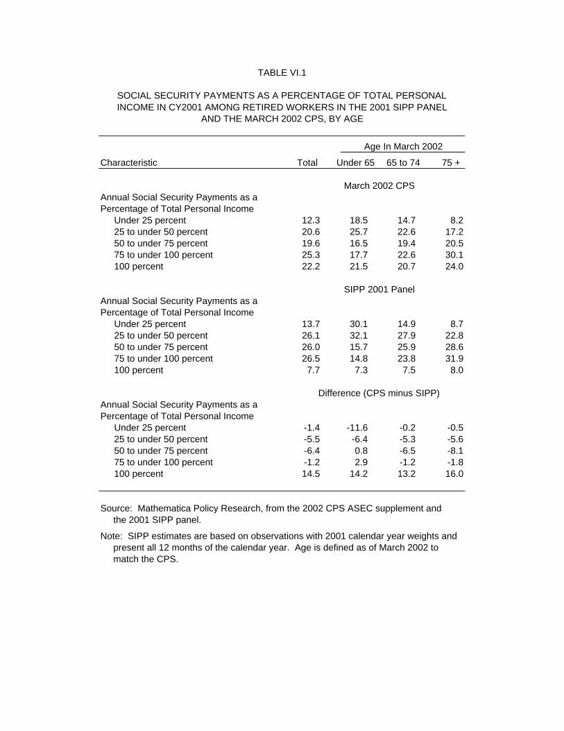
TABLE VI.1

SOCIAL SECURITY PAYMENTS AS A PERCENTAGE OF TOTAL PERSONALINCOME IN CY2001 AMONG RETIRED WORKERS IN THE 2001 SIPP PANEL

AND THE MARCH 2002 CPS, BY AGE

Age In March 2002

Characteristic Total Under 65 65 to 74 75 +

March 2002 CPSAnnual Social Security Payments as a Percentage of Total Personal Income

Under 25 percent 12.3 18.5 14.7 8.225 to under 50 percent 20.6 25.7 22.6 17.250 to under 75 percent 19.6 16.5 19.4 20.575 to under 100 percent 25.3 17.7 22.6 30.1100 percent 22.2 21.5 20.7 24.0

SIPP 2001 PanelAnnual Social Security Payments as a Percentage of Total Personal Income

Under 25 percent 13.7 30.1 14.9 8.725 to under 50 percent 26.1 32.1 27.9 22.850 to under 75 percent 26.0 15.7 25.9 28.675 to under 100 percent 26.5 14.8 23.8 31.9100 percent 7.7 7.3 7.5 8.0

Difference (CPS minus SIPP)Annual Social Security Payments as a Percentage of Total Personal Income

Under 25 percent -1.4 -11.6 -0.2 -0.525 to under 50 percent -5.5 -6.4 -5.3 -5.650 to under 75 percent -6.4 0.8 -6.5 -8.175 to under 100 percent -1.2 2.9 -1.2 -1.8100 percent 14.5 14.2 13.2 16.0

Source: Mathematica Policy Research, from the 2002 CPS ASEC supplement and the 2001 SIPP panel.

Note: SIPP estimates are based on observations with 2001 calendar year weights and present all 12 months of the calendar year. Age is defined as of March 2002 to match the CPS.

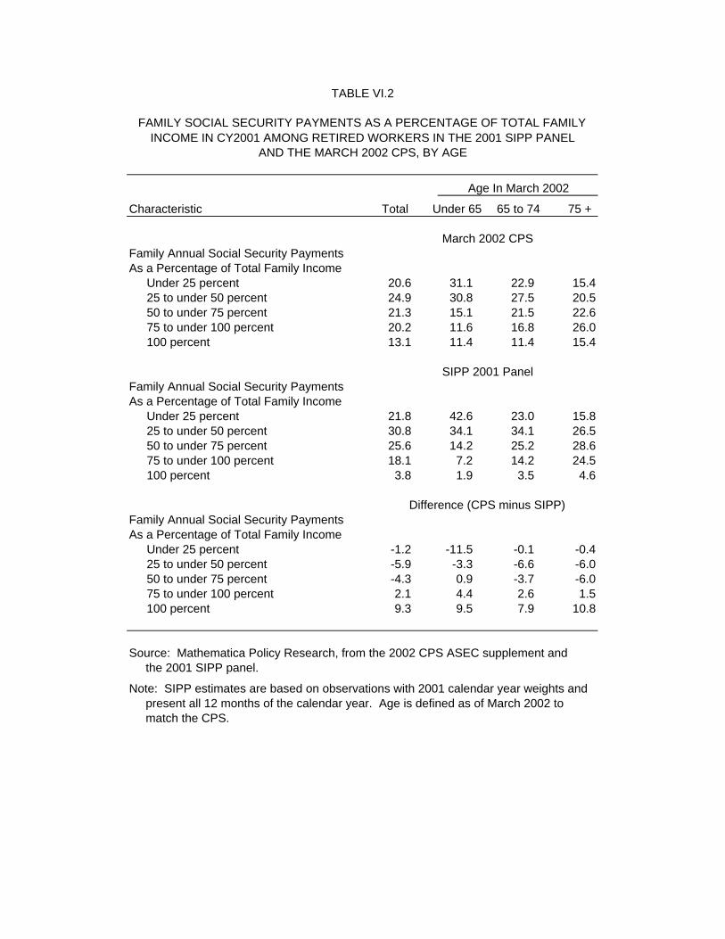
TABLE VI.2

FAMILY SOCIAL SECURITY PAYMENTS AS A PERCENTAGE OF TOTAL FAMILYINCOME IN CY2001 AMONG RETIRED WORKERS IN THE 2001 SIPP PANEL

AND THE MARCH 2002 CPS, BY AGE

Age In March 2002

Characteristic Total Under 65 65 to 74 75 +

March 2002 CPSFamily Annual Social Security PaymentsAs a Percentage of Total Family Income

Under 25 percent 20.6 31.1 22.9 15.425 to under 50 percent 24.9 30.8 27.5 20.550 to under 75 percent 21.3 15.1 21.5 22.675 to under 100 percent 20.2 11.6 16.8 26.0100 percent 13.1 11.4 11.4 15.4

SIPP 2001 PanelFamily Annual Social Security PaymentsAs a Percentage of Total Family Income

Under 25 percent 21.8 42.6 23.0 15.825 to under 50 percent 30.8 34.1 34.1 26.550 to under 75 percent 25.6 14.2 25.2 28.675 to under 100 percent 18.1 7.2 14.2 24.5100 percent 3.8 1.9 3.5 4.6

Difference (CPS minus SIPP)Family Annual Social Security PaymentsAs a Percentage of Total Family Income

Under 25 percent -1.2 -11.5 -0.1 -0.425 to under 50 percent -5.9 -3.3 -6.6 -6.050 to under 75 percent -4.3 0.9 -3.7 -6.075 to under 100 percent 2.1 4.4 2.6 1.5100 percent 9.3 9.5 7.9 10.8

Source: Mathematica Policy Research, from the 2002 CPS ASEC supplement and the 2001 SIPP panel.

Note: SIPP estimates are based on observations with 2001 calendar year weights and present all 12 months of the calendar year. Age is defined as of March 2002 to match the CPS.

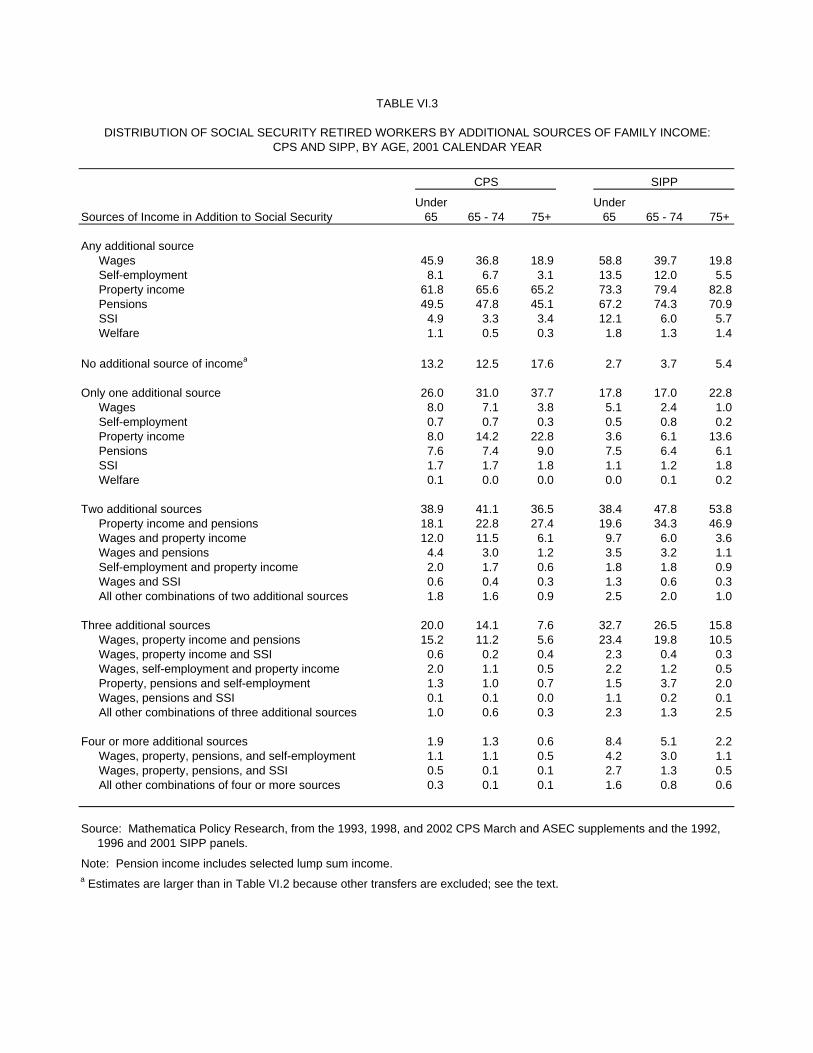
TABLE VI.3

DISTRIBUTION OF SOCIAL SECURITY RETIRED WORKERS BY ADDITIONAL SOURCES OF FAMILY INCOME:CPS AND SIPP, BY AGE, 2001 CALENDAR YEAR

CPS SIPP

Under UnderSources of Income in Addition to Social Security 65 65 - 74 75+ 65 65 - 74 75+

Any additional sourceWages 45.9 36.8 18.9 58.8 39.7 19.8Self-employment 8.1 6.7 3.1 13.5 12.0 5.5Property income 61.8 65.6 65.2 73.3 79.4 82.8Pensions 49.5 47.8 45.1 67.2 74.3 70.9SSI 4.9 3.3 3.4 12.1 6.0 5.7Welfare 1.1 0.5 0.3 1.8 1.3 1.4

No additional source of incomea 13.2 12.5 17.6 2.7 3.7 5.4

Only one additional source 26.0 31.0 37.7 17.8 17.0 22.8Wages 8.0 7.1 3.8 5.1 2.4 1.0Self-employment 0.7 0.7 0.3 0.5 0.8 0.2Property income 8.0 14.2 22.8 3.6 6.1 13.6Pensions 7.6 7.4 9.0 7.5 6.4 6.1SSI 1.7 1.7 1.8 1.1 1.2 1.8Welfare 0.1 0.0 0.0 0.0 0.1 0.2

Two additional sources 38.9 41.1 36.5 38.4 47.8 53.8Property income and pensions 18.1 22.8 27.4 19.6 34.3 46.9Wages and property income 12.0 11.5 6.1 9.7 6.0 3.6Wages and pensions 4.4 3.0 1.2 3.5 3.2 1.1Self-employment and property income 2.0 1.7 0.6 1.8 1.8 0.9Wages and SSI 0.6 0.4 0.3 1.3 0.6 0.3All other combinations of two additional sources 1.8 1.6 0.9 2.5 2.0 1.0

Three additional sources 20.0 14.1 7.6 32.7 26.5 15.8Wages, property income and pensions 15.2 11.2 5.6 23.4 19.8 10.5Wages, property income and SSI 0.6 0.2 0.4 2.3 0.4 0.3Wages, self-employment and property income 2.0 1.1 0.5 2.2 1.2 0.5Property, pensions and self-employment 1.3 1.0 0.7 1.5 3.7 2.0Wages, pensions and SSI 0.1 0.1 0.0 1.1 0.2 0.1All other combinations of three additional sources 1.0 0.6 0.3 2.3 1.3 2.5

Four or more additional sources 1.9 1.3 0.6 8.4 5.1 2.2Wages, property, pensions, and self-employment 1.1 1.1 0.5 4.2 3.0 1.1Wages, property, pensions, and SSI 0.5 0.1 0.1 2.7 1.3 0.5All other combinations of four or more sources 0.3 0.1 0.1 1.6 0.8 0.6

Source: Mathematica Policy Research, from the 1993, 1998, and 2002 CPS March and ASEC supplements and the 1992, 1996 and 2001 SIPP panels.

Note: Pension income includes selected lump sum income.a Estimates are larger than in Table VI.2 because other transfers are excluded; see the text.

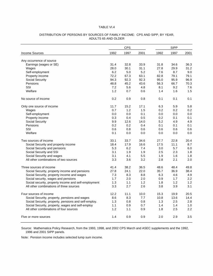
TABLE VI.4

DISTRIBUTION OF PERSONS BY SOURCES OF FAMILY INCOME: CPS AND SIPP, BY YEAR,ADULTS 65 AND OLDER

CPS SIPP

Income Sources 1992 1997 2001 1992 1997 2001

Any occurrence of sourceEarnings (wages or SE) 31.4 32.8 33.9 31.8 34.6 36.3Wages 28.0 30.1 31.1 27.8 29.9 31.2Self-employment 6.2 5.0 5.2 7.6 8.7 9.0Property income 72.2 67.3 63.1 82.8 79.1 79.1Social Security 94.3 92.3 92.3 95.0 95.9 96.9Pensions 48.8 45.2 43.6 56.3 66.7 70.3SSI 7.2 5.6 4.8 8.1 9.2 7.6Welfare 1.2 0.7 0.6 1.4 1.6 1.5

No source of income 0.2 0.9 0.8 0.1 0.1 0.1

Only one source of income 11.7 15.2 17.1 6.3 5.9 5.8Wages 0.7 1.2 1.5 0.2 0.2 0.2Self-employment 0.0 0.0 0.1 0.0 0.0 0.0Property income 0.3 0.4 0.5 0.2 0.1 0.1Social Security 9.9 12.6 14.0 5.2 4.9 4.9Pensions 0.2 0.2 0.4 0.1 0.1 0.1SSI 0.6 0.8 0.6 0.6 0.6 0.6Welfare 0.1 0.0 0.0 0.0 0.0 0.0

Two sources of income 33.1 33.7 34.6 27.7 22.8 20.4Social Security and property income 18.4 17.9 16.6 17.5 11.1 8.7Social Security and pensions 5.3 6.2 7.4 3.0 5.7 6.0Social Security and SSI 3.1 1.9 1.9 2.5 2.3 1.8Social Security and wages 3.1 4.1 5.5 1.9 1.6 1.8All other combinations of two sources 3.3 3.6 3.2 2.8 2.1 2.0

Three sources of income 41.4 38.2 36.5 48.6 48.4 49.8Social Security, property income and pensions 27.8 24.1 22.0 35.7 36.9 38.4Social Security, property income and wages 7.3 8.3 8.8 6.3 4.6 4.9Social security, wages and pensions 1.7 2.0 2.0 0.9 1.7 2.2Social security, property income and self-employment 1.3 1.1 1.2 1.8 1.2 1.2All other combinations of three sources 3.3 2.7 2.6 3.8 3.9 3.1

Four sources of income 12.2 11.1 10.0 15.3 19.9 20.5Social Security, property, pensions and wages 8.6 8.3 7.7 10.8 13.6 14.4Social Security, property, pensions and self-employ. 1.3 0.8 0.8 1.3 2.5 2.8Social Security, property, wages and self-employ 1.1 0.9 0.7 1.4 1.4 1.0All other combinations of four sources 1.2 1.1 0.9 1.8 2.5 2.2

Five or more sources 1.4 0.9 0.9 2.0 2.9 3.5

Source: Mathematica Policy Research, from the 1993, 1998, and 2002 CPS March and ASEC supplements and the 1992, 1996 and 2001 SIPP panels.

Note: Pension income includes selected lump sum income.

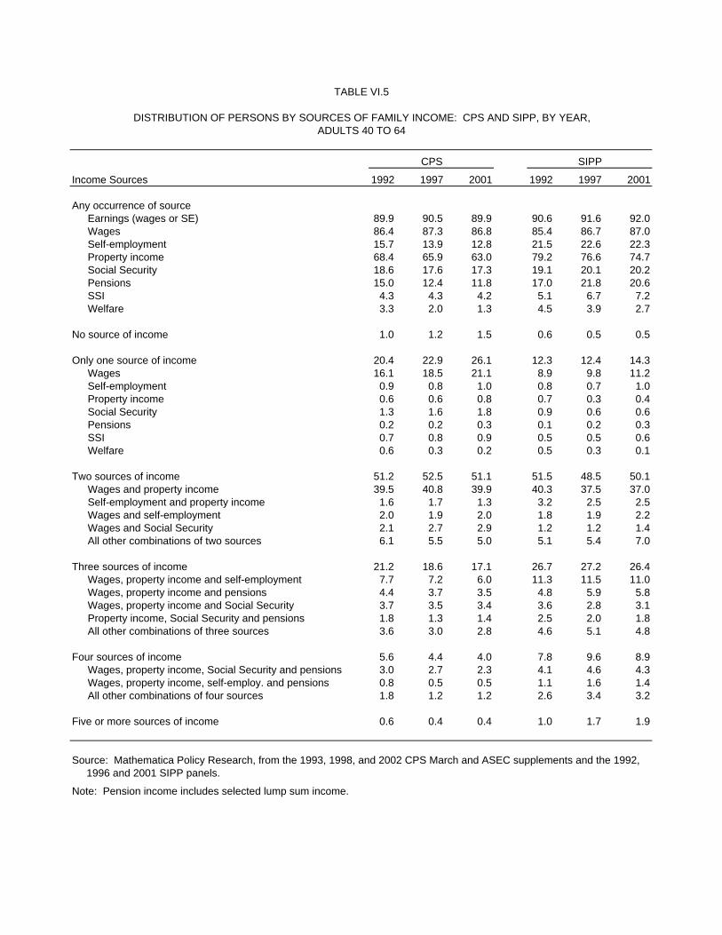
TABLE VI.5

DISTRIBUTION OF PERSONS BY SOURCES OF FAMILY INCOME: CPS AND SIPP, BY YEAR,ADULTS 40 TO 64

CPS SIPP

Income Sources 1992 1997 2001 1992 1997 2001

Any occurrence of sourceEarnings (wages or SE) 89.9 90.5 89.9 90.6 91.6 92.0Wages 86.4 87.3 86.8 85.4 86.7 87.0Self-employment 15.7 13.9 12.8 21.5 22.6 22.3Property income 68.4 65.9 63.0 79.2 76.6 74.7Social Security 18.6 17.6 17.3 19.1 20.1 20.2Pensions 15.0 12.4 11.8 17.0 21.8 20.6SSI 4.3 4.3 4.2 5.1 6.7 7.2Welfare 3.3 2.0 1.3 4.5 3.9 2.7

No source of income 1.0 1.2 1.5 0.6 0.5 0.5

Only one source of income 20.4 22.9 26.1 12.3 12.4 14.3Wages 16.1 18.5 21.1 8.9 9.8 11.2Self-employment 0.9 0.8 1.0 0.8 0.7 1.0Property income 0.6 0.6 0.8 0.7 0.3 0.4Social Security 1.3 1.6 1.8 0.9 0.6 0.6Pensions 0.2 0.2 0.3 0.1 0.2 0.3SSI 0.7 0.8 0.9 0.5 0.5 0.6Welfare 0.6 0.3 0.2 0.5 0.3 0.1

Two sources of income 51.2 52.5 51.1 51.5 48.5 50.1Wages and property income 39.5 40.8 39.9 40.3 37.5 37.0Self-employment and property income 1.6 1.7 1.3 3.2 2.5 2.5Wages and self-employment 2.0 1.9 2.0 1.8 1.9 2.2Wages and Social Security 2.1 2.7 2.9 1.2 1.2 1.4All other combinations of two sources 6.1 5.5 5.0 5.1 5.4 7.0

Three sources of income 21.2 18.6 17.1 26.7 27.2 26.4Wages, property income and self-employment 7.7 7.2 6.0 11.3 11.5 11.0Wages, property income and pensions 4.4 3.7 3.5 4.8 5.9 5.8Wages, property income and Social Security 3.7 3.5 3.4 3.6 2.8 3.1Property income, Social Security and pensions 1.8 1.3 1.4 2.5 2.0 1.8All other combinations of three sources 3.6 3.0 2.8 4.6 5.1 4.8

Four sources of income 5.6 4.4 4.0 7.8 9.6 8.9Wages, property income, Social Security and pensions 3.0 2.7 2.3 4.1 4.6 4.3Wages, property income, self-employ. and pensions 0.8 0.5 0.5 1.1 1.6 1.4All other combinations of four sources 1.8 1.2 1.2 2.6 3.4 3.2

Five or more sources of income 0.6 0.4 0.4 1.0 1.7 1.9

Source: Mathematica Policy Research, from the 1993, 1998, and 2002 CPS March and ASEC supplements and the 1992, 1996 and 2001 SIPP panels.

Note: Pension income includes selected lump sum income.

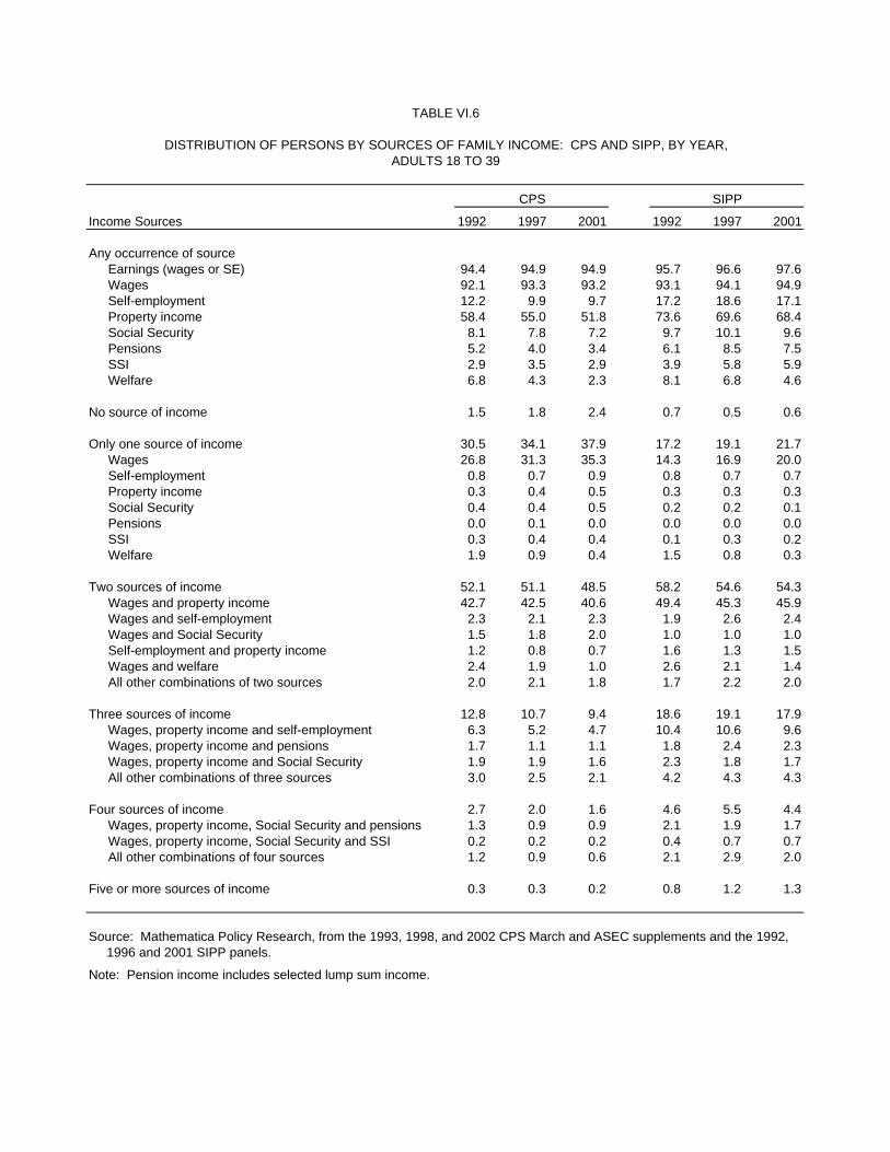
TABLE VI.6

DISTRIBUTION OF PERSONS BY SOURCES OF FAMILY INCOME: CPS AND SIPP, BY YEAR,ADULTS 18 TO 39

CPS SIPP

Income Sources 1992 1997 2001 1992 1997 2001

Any occurrence of sourceEarnings (wages or SE) 94.4 94.9 94.9 95.7 96.6 97.6Wages 92.1 93.3 93.2 93.1 94.1 94.9Self-employment 12.2 9.9 9.7 17.2 18.6 17.1Property income 58.4 55.0 51.8 73.6 69.6 68.4Social Security 8.1 7.8 7.2 9.7 10.1 9.6Pensions 5.2 4.0 3.4 6.1 8.5 7.5SSI 2.9 3.5 2.9 3.9 5.8 5.9Welfare 6.8 4.3 2.3 8.1 6.8 4.6

No source of income 1.5 1.8 2.4 0.7 0.5 0.6

Only one source of income 30.5 34.1 37.9 17.2 19.1 21.7Wages 26.8 31.3 35.3 14.3 16.9 20.0Self-employment 0.8 0.7 0.9 0.8 0.7 0.7Property income 0.3 0.4 0.5 0.3 0.3 0.3Social Security 0.4 0.4 0.5 0.2 0.2 0.1Pensions 0.0 0.1 0.0 0.0 0.0 0.0SSI 0.3 0.4 0.4 0.1 0.3 0.2Welfare 1.9 0.9 0.4 1.5 0.8 0.3

Two sources of income 52.1 51.1 48.5 58.2 54.6 54.3Wages and property income 42.7 42.5 40.6 49.4 45.3 45.9Wages and self-employment 2.3 2.1 2.3 1.9 2.6 2.4Wages and Social Security 1.5 1.8 2.0 1.0 1.0 1.0Self-employment and property income 1.2 0.8 0.7 1.6 1.3 1.5Wages and welfare 2.4 1.9 1.0 2.6 2.1 1.4All other combinations of two sources 2.0 2.1 1.8 1.7 2.2 2.0

Three sources of income 12.8 10.7 9.4 18.6 19.1 17.9Wages, property income and self-employment 6.3 5.2 4.7 10.4 10.6 9.6Wages, property income and pensions 1.7 1.1 1.1 1.8 2.4 2.3Wages, property income and Social Security 1.9 1.9 1.6 2.3 1.8 1.7All other combinations of three sources 3.0 2.5 2.1 4.2 4.3 4.3

Four sources of income 2.7 2.0 1.6 4.6 5.5 4.4Wages, property income, Social Security and pensions 1.3 0.9 0.9 2.1 1.9 1.7Wages, property income, Social Security and SSI 0.2 0.2 0.2 0.4 0.7 0.7All other combinations of four sources 1.2 0.9 0.6 2.1 2.9 2.0

Five or more sources of income 0.3 0.3 0.2 0.8 1.2 1.3

Source: Mathematica Policy Research, from the 1993, 1998, and 2002 CPS March and ASEC supplements and the 1992, 1996 and 2001 SIPP panels.

Note: Pension income includes selected lump sum income.

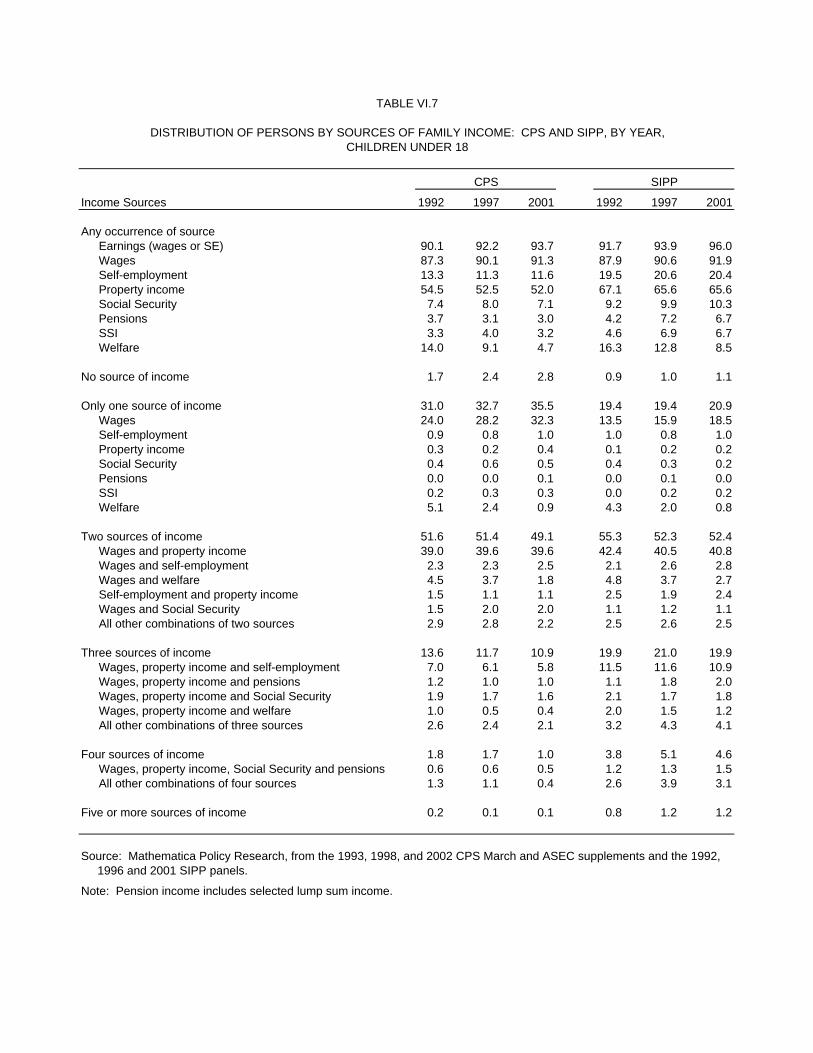
TABLE VI.7

DISTRIBUTION OF PERSONS BY SOURCES OF FAMILY INCOME: CPS AND SIPP, BY YEAR,CHILDREN UNDER 18

CPS SIPP

Income Sources 1992 1997 2001 1992 1997 2001

Any occurrence of sourceEarnings (wages or SE) 90.1 92.2 93.7 91.7 93.9 96.0Wages 87.3 90.1 91.3 87.9 90.6 91.9Self-employment 13.3 11.3 11.6 19.5 20.6 20.4Property income 54.5 52.5 52.0 67.1 65.6 65.6Social Security 7.4 8.0 7.1 9.2 9.9 10.3Pensions 3.7 3.1 3.0 4.2 7.2 6.7SSI 3.3 4.0 3.2 4.6 6.9 6.7Welfare 14.0 9.1 4.7 16.3 12.8 8.5

No source of income 1.7 2.4 2.8 0.9 1.0 1.1

Only one source of income 31.0 32.7 35.5 19.4 19.4 20.9Wages 24.0 28.2 32.3 13.5 15.9 18.5Self-employment 0.9 0.8 1.0 1.0 0.8 1.0Property income 0.3 0.2 0.4 0.1 0.2 0.2Social Security 0.4 0.6 0.5 0.4 0.3 0.2Pensions 0.0 0.0 0.1 0.0 0.1 0.0SSI 0.2 0.3 0.3 0.0 0.2 0.2Welfare 5.1 2.4 0.9 4.3 2.0 0.8

Two sources of income 51.6 51.4 49.1 55.3 52.3 52.4Wages and property income 39.0 39.6 39.6 42.4 40.5 40.8Wages and self-employment 2.3 2.3 2.5 2.1 2.6 2.8Wages and welfare 4.5 3.7 1.8 4.8 3.7 2.7Self-employment and property income 1.5 1.1 1.1 2.5 1.9 2.4Wages and Social Security 1.5 2.0 2.0 1.1 1.2 1.1All other combinations of two sources 2.9 2.8 2.2 2.5 2.6 2.5

Three sources of income 13.6 11.7 10.9 19.9 21.0 19.9Wages, property income and self-employment 7.0 6.1 5.8 11.5 11.6 10.9Wages, property income and pensions 1.2 1.0 1.0 1.1 1.8 2.0Wages, property income and Social Security 1.9 1.7 1.6 2.1 1.7 1.8Wages, property income and welfare 1.0 0.5 0.4 2.0 1.5 1.2All other combinations of three sources 2.6 2.4 2.1 3.2 4.3 4.1

Four sources of income 1.8 1.7 1.0 3.8 5.1 4.6Wages, property income, Social Security and pensions 0.6 0.6 0.5 1.2 1.3 1.5All other combinations of four sources 1.3 1.1 0.4 2.6 3.9 3.1

Five or more sources of income 0.2 0.1 0.1 0.8 1.2 1.2

Source: Mathematica Policy Research, from the 1993, 1998, and 2002 CPS March and ASEC supplements and the 1992, 1996 and 2001 SIPP panels.

Note: Pension income includes selected lump sum income.

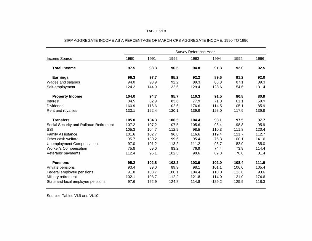
TABLE VI.8

SIPP AGGREGATE INCOME AS A PERCENTAGE OF MARCH CPS AGGREGATE INCOME, 1990 TO 1996

Survey Reference Year

Income Source 1990 1991 1992 1993 1994 1995 1996

Total Income 97.5 98.3 96.5 94.8 91.3 92.0 92.5

Earnings 96.3 97.7 95.2 92.2 89.6 91.2 92.0Wages and salaries 94.0 93.9 92.2 89.3 86.8 87.1 89.3Self-employment 124.2 144.9 132.6 129.4 128.6 154.6 131.4

Property Income 104.0 94.7 95.7 110.3 91.5 80.8 80.9Interest 84.5 82.9 83.6 77.9 71.0 61.1 59.9Dividends 160.9 116.6 102.6 176.6 114.5 105.1 85.9Rent and royalties 133.1 122.4 130.1 139.9 125.0 117.9 139.9

Transfers 105.0 104.3 106.5 104.4 98.1 97.5 97.7Social Security and Railroad Retirement 107.2 107.2 107.5 105.6 98.4 98.8 95.9SSI 105.3 104.7 112.5 98.5 110.3 111.8 120.4Family Assistance 101.6 102.7 96.8 116.6 119.4 121.7 112.7Other cash welfare 95.7 130.2 99.6 95.4 75.3 100.1 141.6Unemployment Compensation 97.0 101.2 113.2 111.2 93.7 82.9 85.0Worker’s Compensation 75.8 69.0 83.2 76.9 74.4 73.9 114.4Veterans’ payments 112.4 95.1 102.3 90.6 89.3 76.6 81.4

Pensions 95.2 102.8 102.2 103.9 102.0 108.4 111.9Private pensions 93.4 89.0 89.9 98.1 101.1 106.0 105.4Federal employee pensions 91.8 108.7 100.1 104.4 110.0 113.6 93.6Military retirement 102.1 108.7 112.2 121.8 114.0 121.0 174.6State and local employee pensions 97.6 122.9 124.8 114.8 129.2 125.9 118.3

Source: Tables VI.9 and VI.10.

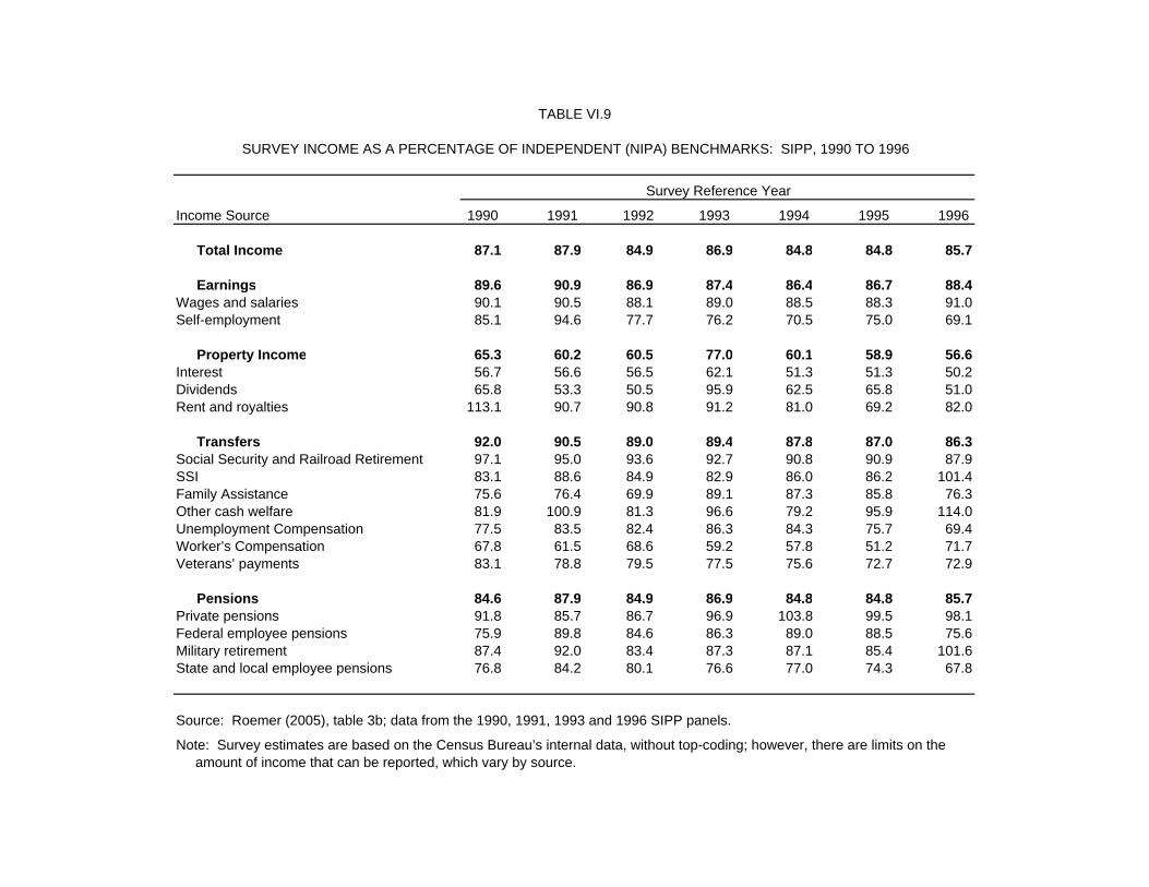
TABLE VI.9

SURVEY INCOME AS A PERCENTAGE OF INDEPENDENT (NIPA) BENCHMARKS: SIPP, 1990 TO 1996

Survey Reference Year

Income Source 1990 1991 1992 1993 1994 1995 1996

Total Income 87.1 87.9 84.9 86.9 84.8 84.8 85.7

Earnings 89.6 90.9 86.9 87.4 86.4 86.7 88.4Wages and salaries 90.1 90.5 88.1 89.0 88.5 88.3 91.0Self-employment 85.1 94.6 77.7 76.2 70.5 75.0 69.1

Property Income 65.3 60.2 60.5 77.0 60.1 58.9 56.6Interest 56.7 56.6 56.5 62.1 51.3 51.3 50.2Dividends 65.8 53.3 50.5 95.9 62.5 65.8 51.0Rent and royalties 113.1 90.7 90.8 91.2 81.0 69.2 82.0

Transfers 92.0 90.5 89.0 89.4 87.8 87.0 86.3Social Security and Railroad Retirement 97.1 95.0 93.6 92.7 90.8 90.9 87.9SSI 83.1 88.6 84.9 82.9 86.0 86.2 101.4Family Assistance 75.6 76.4 69.9 89.1 87.3 85.8 76.3Other cash welfare 81.9 100.9 81.3 96.6 79.2 95.9 114.0Unemployment Compensation 77.5 83.5 82.4 86.3 84.3 75.7 69.4Worker’s Compensation 67.8 61.5 68.6 59.2 57.8 51.2 71.7Veterans’ payments 83.1 78.8 79.5 77.5 75.6 72.7 72.9

Pensions 84.6 87.9 84.9 86.9 84.8 84.8 85.7Private pensions 91.8 85.7 86.7 96.9 103.8 99.5 98.1Federal employee pensions 75.9 89.8 84.6 86.3 89.0 88.5 75.6Military retirement 87.4 92.0 83.4 87.3 87.1 85.4 101.6State and local employee pensions 76.8 84.2 80.1 76.6 77.0 74.3 67.8

Source: Roemer (2005), table 3b; data from the 1990, 1991, 1993 and 1996 SIPP panels.

Note: Survey estimates are based on the Census Bureau’s internal data, without top-coding; however, there are limits on the amount of income that can be reported, which vary by source.

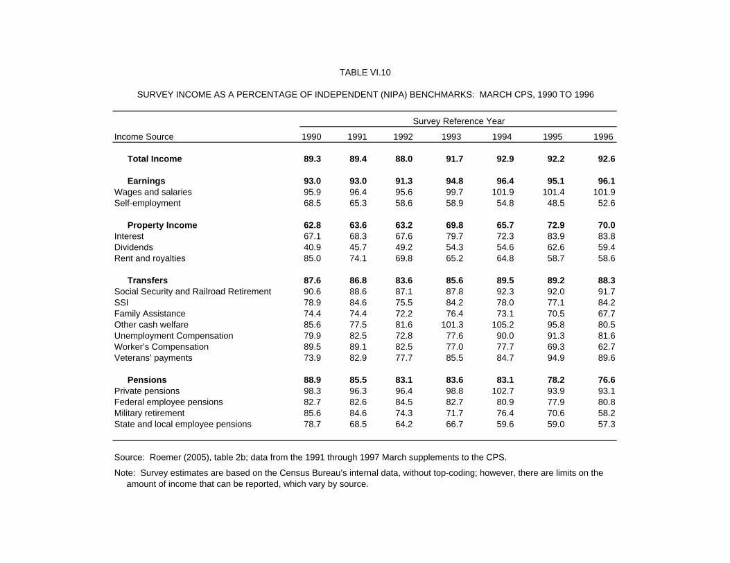
TABLE VI.10

SURVEY INCOME AS A PERCENTAGE OF INDEPENDENT (NIPA) BENCHMARKS: MARCH CPS, 1990 TO 1996

Survey Reference Year

Income Source 1990 1991 1992 1993 1994 1995 1996

Total Income 89.3 89.4 88.0 91.7 92.9 92.2 92.6

Earnings 93.0 93.0 91.3 94.8 96.4 95.1 96.1Wages and salaries 95.9 96.4 95.6 99.7 101.9 101.4 101.9Self-employment 68.5 65.3 58.6 58.9 54.8 48.5 52.6

Property Income 62.8 63.6 63.2 69.8 65.7 72.9 70.0Interest 67.1 68.3 67.6 79.7 72.3 83.9 83.8Dividends 40.9 45.7 49.2 54.3 54.6 62.6 59.4Rent and royalties 85.0 74.1 69.8 65.2 64.8 58.7 58.6

Transfers 87.6 86.8 83.6 85.6 89.5 89.2 88.3Social Security and Railroad Retirement 90.6 88.6 87.1 87.8 92.3 92.0 91.7SSI 78.9 84.6 75.5 84.2 78.0 77.1 84.2Family Assistance 74.4 74.4 72.2 76.4 73.1 70.5 67.7Other cash welfare 85.6 77.5 81.6 101.3 105.2 95.8 80.5Unemployment Compensation 79.9 82.5 72.8 77.6 90.0 91.3 81.6Worker’s Compensation 89.5 89.1 82.5 77.0 77.7 69.3 62.7Veterans’ payments 73.9 82.9 77.7 85.5 84.7 94.9 89.6

Pensions 88.9 85.5 83.1 83.6 83.1 78.2 76.6Private pensions 98.3 96.3 96.4 98.8 102.7 93.9 93.1Federal employee pensions 82.7 82.6 84.5 82.7 80.9 77.9 80.8Military retirement 85.6 84.6 74.3 71.7 76.4 70.6 58.2State and local employee pensions 78.7 68.5 64.2 66.7 59.6 59.0 57.3

Source: Roemer (2005), table 2b; data from the 1991 through 1997 March supplements to the CPS.

Note: Survey estimates are based on the Census Bureau’s internal data, without top-coding; however, there are limits on the amount of income that can be reported, which vary by source.

TABLE VI.11

COMPARISON OF SIPP AND CPS AGGREGATE AMOUNTS OF INCOME FOR SELECTED YEARS BY SOURCE:ALL FAMILY INCOME QUINTILES

SIPP Aggregate ($Billions) CPS Aggregate ($Billions) SIPP as Percent of CPS

Income Source 1993 1997 2002 1993 1997 2002 1993 1997 2002

Total Income 3,643.5 4,571.0 5,783.0 3,854.8 5,138.0 6,468.4 94.5 89.0 89.4

Wages and Salaries 2,522.1 3,232.2 4,142.5 2,837.1 3,819.8 5,026.3 88.9 84.6 82.4Self-Employment 341.9 491.2 617.6 213.3 296.7 328.0 160.3 165.6 188.3Property Income 188.6 168.6 138.8 226.0 344.1 265.1 83.5 49.0 52.3Social Security and Railroad Retirement 257.7 299.3 371.5 252.0 319.7 389.6 102.2 93.6 95.4SSI 18.2 28.7 33.9 18.5 22.7 25.8 98.2 126.5 131.5Welfare 19.9 17.6 9.4 20.4 12.1 6.4 97.6 145.0 146.7Other Transfers 109.2 69.2 103.3 124.2 126.4 178.1 87.9 54.7 58.0Pensions 185.9 264.3 365.9 163.2 196.4 249.0 113.9 134.5 147.0

Source: Mathematica Policy Research, from the 1992, 1996, and 2001 SIPP panels and the 1993, 1998, and 2003 CPS March and ASEC supplements.

Note: All income from families with Armed Forces members is excluded. Pension amounts include lump sum payments requested in both surveys. Other transfers include other cash welfare, unemployment compensation, worker’s compensation, and veterans’ payments.

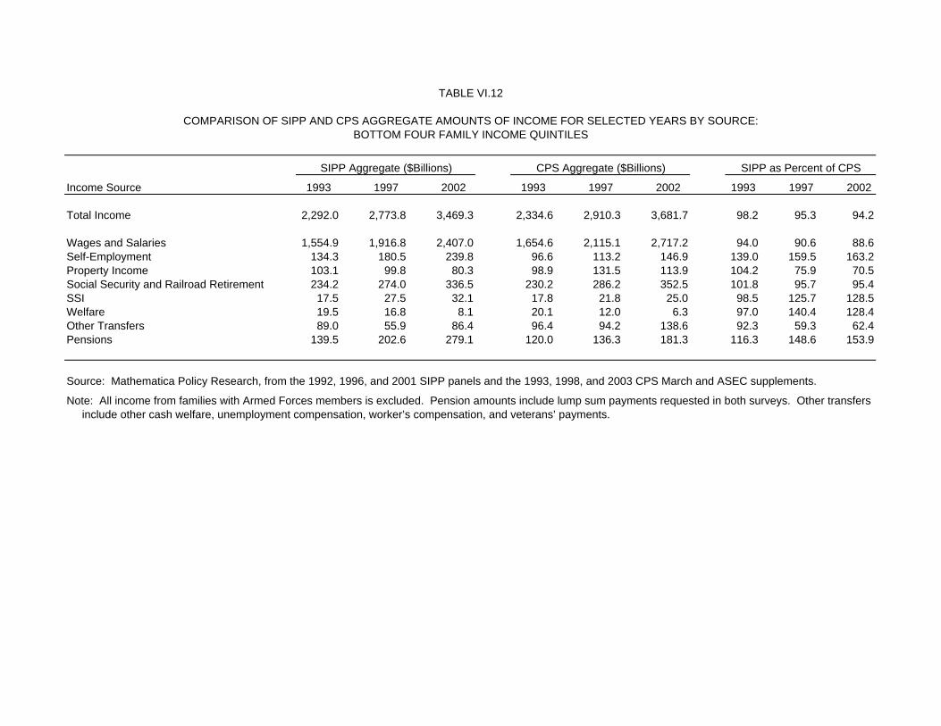
TABLE VI.12

COMPARISON OF SIPP AND CPS AGGREGATE AMOUNTS OF INCOME FOR SELECTED YEARS BY SOURCE:BOTTOM FOUR FAMILY INCOME QUINTILES

SIPP Aggregate ($Billions) CPS Aggregate ($Billions) SIPP as Percent of CPS

Income Source 1993 1997 2002 1993 1997 2002 1993 1997 2002

Total Income 2,292.0 2,773.8 3,469.3 2,334.6 2,910.3 3,681.7 98.2 95.3 94.2

Wages and Salaries 1,554.9 1,916.8 2,407.0 1,654.6 2,115.1 2,717.2 94.0 90.6 88.6Self-Employment 134.3 180.5 239.8 96.6 113.2 146.9 139.0 159.5 163.2Property Income 103.1 99.8 80.3 98.9 131.5 113.9 104.2 75.9 70.5Social Security and Railroad Retirement 234.2 274.0 336.5 230.2 286.2 352.5 101.8 95.7 95.4SSI 17.5 27.5 32.1 17.8 21.8 25.0 98.5 125.7 128.5Welfare 19.5 16.8 8.1 20.1 12.0 6.3 97.0 140.4 128.4Other Transfers 89.0 55.9 86.4 96.4 94.2 138.6 92.3 59.3 62.4Pensions 139.5 202.6 279.1 120.0 136.3 181.3 116.3 148.6 153.9

Source: Mathematica Policy Research, from the 1992, 1996, and 2001 SIPP panels and the 1993, 1998, and 2003 CPS March and ASEC supplements.

Note: All income from families with Armed Forces members is excluded. Pension amounts include lump sum payments requested in both surveys. Other transfers include other cash welfare, unemployment compensation, worker’s compensation, and veterans’ payments.

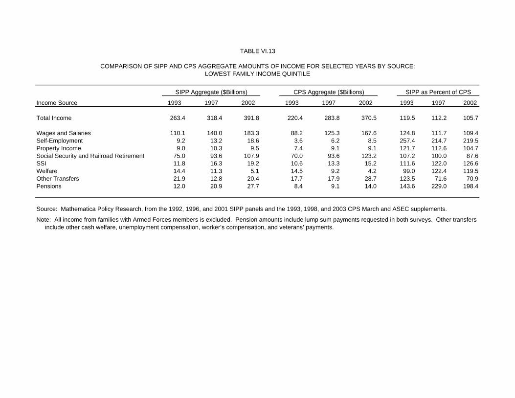
TABLE VI.13

COMPARISON OF SIPP AND CPS AGGREGATE AMOUNTS OF INCOME FOR SELECTED YEARS BY SOURCE:LOWEST FAMILY INCOME QUINTILE

SIPP Aggregate ($Billions) CPS Aggregate ($Billions) SIPP as Percent of CPS

Income Source 1993 1997 2002 1993 1997 2002 1993 1997 2002

Total Income 263.4 318.4 391.8 220.4 283.8 370.5 119.5 112.2 105.7

Wages and Salaries 110.1 140.0 183.3 88.2 125.3 167.6 124.8 111.7 109.4Self-Employment 9.2 13.2 18.6 3.6 6.2 8.5 257.4 214.7 219.5Property Income 9.0 10.3 9.5 7.4 9.1 9.1 121.7 112.6 104.7Social Security and Railroad Retirement 75.0 93.6 107.9 70.0 93.6 123.2 107.2 100.0 87.6SSI 11.8 16.3 19.2 10.6 13.3 15.2 111.6 122.0 126.6Welfare 14.4 11.3 5.1 14.5 9.2 4.2 99.0 122.4 119.5Other Transfers 21.9 12.8 20.4 17.7 17.9 28.7 123.5 71.6 70.9Pensions 12.0 20.9 27.7 8.4 9.1 14.0 143.6 229.0 198.4

Source: Mathematica Policy Research, from the 1992, 1996, and 2001 SIPP panels and the 1993, 1998, and 2003 CPS March and ASEC supplements.

Note: All income from families with Armed Forces members is excluded. Pension amounts include lump sum payments requested in both surveys. Other transfers include other cash welfare, unemployment compensation, worker’s compensation, and veterans’ payments.

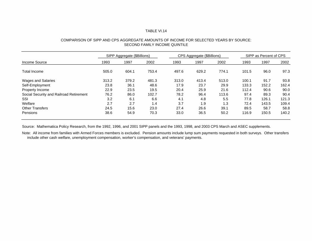
TABLE VI.14

COMPARISON OF SIPP AND CPS AGGREGATE AMOUNTS OF INCOME FOR SELECTED YEARS BY SOURCE:SECOND FAMILY INCOME QUINTILE

SIPP Aggregate ($Billions) CPS Aggregate ($Billions) SIPP as Percent of CPS

Income Source 1993 1997 2002 1993 1997 2002 1993 1997 2002

Total Income 505.0 604.1 753.4 497.6 629.2 774.1 101.5 96.0 97.3

Wages and Salaries 313.2 379.2 481.3 313.0 413.4 513.0 100.1 91.7 93.8Self-Employment 23.8 36.1 48.6 17.9 23.7 29.9 133.3 152.2 162.4Property Income 22.9 23.5 19.5 20.4 25.9 21.6 112.4 90.6 90.0Social Security and Railroad Retirement 76.2 86.0 102.7 78.2 96.4 113.6 97.4 89.3 90.4SSI 3.2 6.1 6.6 4.1 4.8 5.5 77.8 126.1 121.3Welfare 2.7 2.7 1.4 3.7 1.9 1.3 72.4 143.5 109.4Other Transfers 24.5 15.6 23.0 27.4 26.6 39.1 89.5 58.7 58.8Pensions 38.6 54.9 70.3 33.0 36.5 50.2 116.9 150.5 140.2

Source: Mathematica Policy Research, from the 1992, 1996, and 2001 SIPP panels and the 1993, 1998, and 2003 CPS March and ASEC supplements.

Note: All income from families with Armed Forces members is excluded. Pension amounts include lump sum payments requested in both surveys. Other transfers include other cash welfare, unemployment compensation, worker’s compensation, and veterans’ payments.

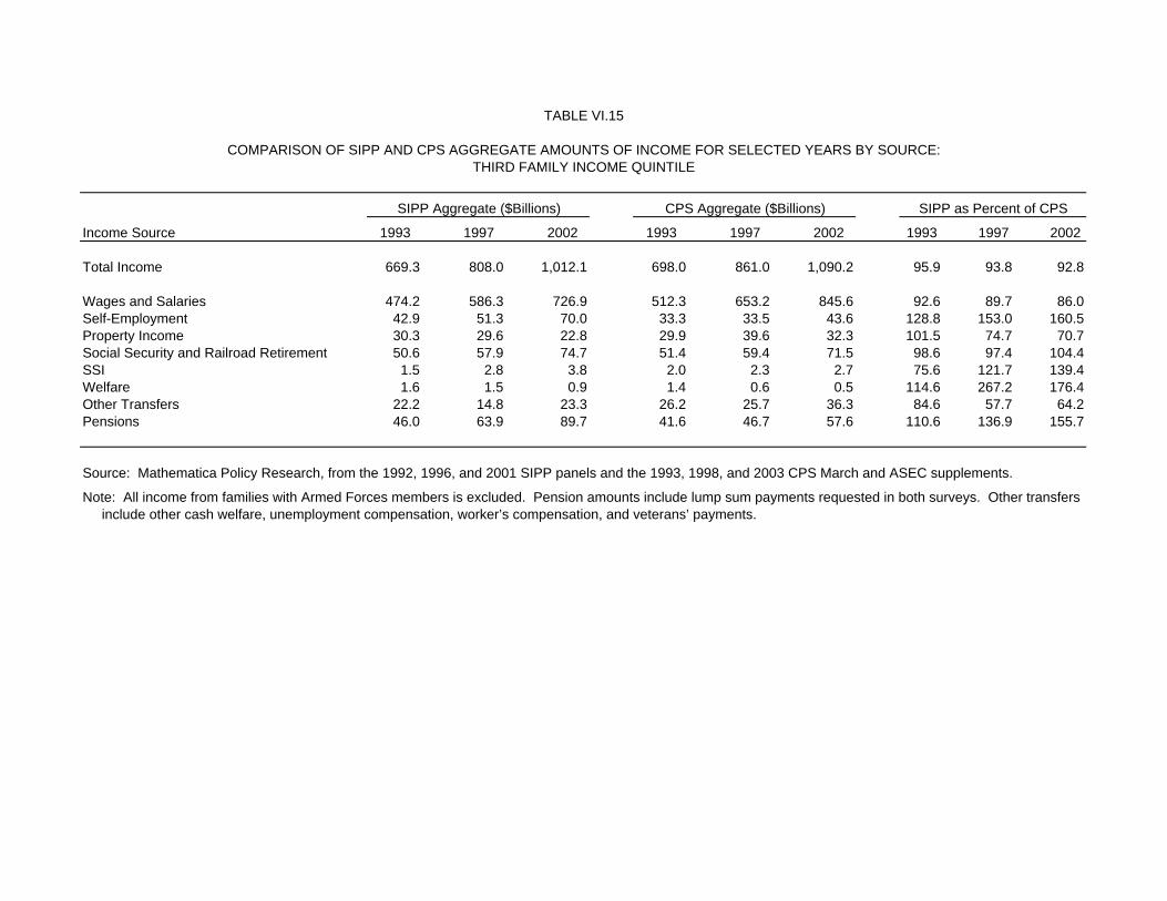
TABLE VI.15

COMPARISON OF SIPP AND CPS AGGREGATE AMOUNTS OF INCOME FOR SELECTED YEARS BY SOURCE:THIRD FAMILY INCOME QUINTILE

SIPP Aggregate ($Billions) CPS Aggregate ($Billions) SIPP as Percent of CPS

Income Source 1993 1997 2002 1993 1997 2002 1993 1997 2002

Total Income 669.3 808.0 1,012.1 698.0 861.0 1,090.2 95.9 93.8 92.8

Wages and Salaries 474.2 586.3 726.9 512.3 653.2 845.6 92.6 89.7 86.0Self-Employment 42.9 51.3 70.0 33.3 33.5 43.6 128.8 153.0 160.5Property Income 30.3 29.6 22.8 29.9 39.6 32.3 101.5 74.7 70.7Social Security and Railroad Retirement 50.6 57.9 74.7 51.4 59.4 71.5 98.6 97.4 104.4SSI 1.5 2.8 3.8 2.0 2.3 2.7 75.6 121.7 139.4Welfare 1.6 1.5 0.9 1.4 0.6 0.5 114.6 267.2 176.4Other Transfers 22.2 14.8 23.3 26.2 25.7 36.3 84.6 57.7 64.2Pensions 46.0 63.9 89.7 41.6 46.7 57.6 110.6 136.9 155.7

Source: Mathematica Policy Research, from the 1992, 1996, and 2001 SIPP panels and the 1993, 1998, and 2003 CPS March and ASEC supplements.

Note: All income from families with Armed Forces members is excluded. Pension amounts include lump sum payments requested in both surveys. Other transfers include other cash welfare, unemployment compensation, worker’s compensation, and veterans’ payments.

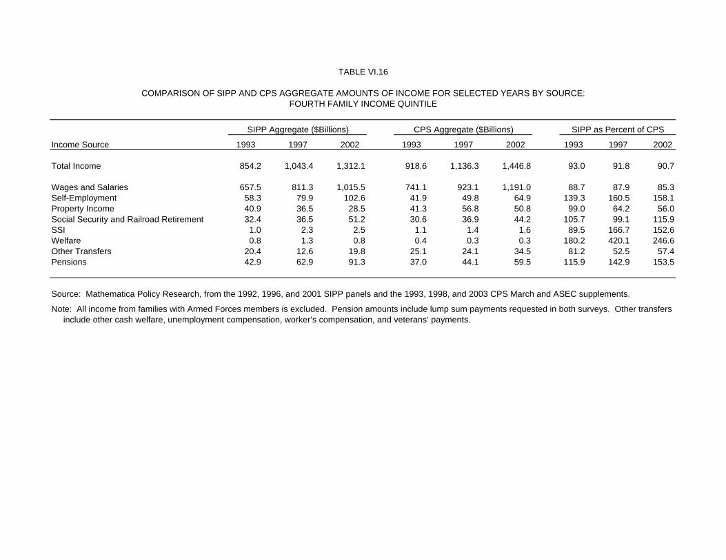
TABLE VI.16

COMPARISON OF SIPP AND CPS AGGREGATE AMOUNTS OF INCOME FOR SELECTED YEARS BY SOURCE:FOURTH FAMILY INCOME QUINTILE

SIPP Aggregate ($Billions) CPS Aggregate ($Billions) SIPP as Percent of CPS

Income Source 1993 1997 2002 1993 1997 2002 1993 1997 2002

Total Income 854.2 1,043.4 1,312.1 918.6 1,136.3 1,446.8 93.0 91.8 90.7

Wages and Salaries 657.5 811.3 1,015.5 741.1 923.1 1,191.0 88.7 87.9 85.3Self-Employment 58.3 79.9 102.6 41.9 49.8 64.9 139.3 160.5 158.1Property Income 40.9 36.5 28.5 41.3 56.8 50.8 99.0 64.2 56.0Social Security and Railroad Retirement 32.4 36.5 51.2 30.6 36.9 44.2 105.7 99.1 115.9SSI 1.0 2.3 2.5 1.1 1.4 1.6 89.5 166.7 152.6Welfare 0.8 1.3 0.8 0.4 0.3 0.3 180.2 420.1 246.6Other Transfers 20.4 12.6 19.8 25.1 24.1 34.5 81.2 52.5 57.4Pensions 42.9 62.9 91.3 37.0 44.1 59.5 115.9 142.9 153.5

Source: Mathematica Policy Research, from the 1992, 1996, and 2001 SIPP panels and the 1993, 1998, and 2003 CPS March and ASEC supplements.

Note: All income from families with Armed Forces members is excluded. Pension amounts include lump sum payments requested in both surveys. Other transfers include other cash welfare, unemployment compensation, worker’s compensation, and veterans’ payments.

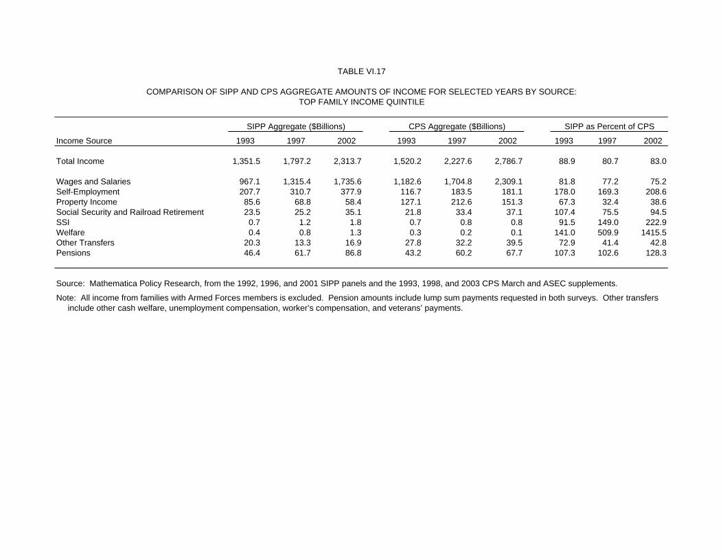
TABLE VI.17

COMPARISON OF SIPP AND CPS AGGREGATE AMOUNTS OF INCOME FOR SELECTED YEARS BY SOURCE:TOP FAMILY INCOME QUINTILE

SIPP Aggregate ($Billions) CPS Aggregate ($Billions) SIPP as Percent of CPS

Income Source 1993 1997 2002 1993 1997 2002 1993 1997 2002

Total Income 1,351.5 1,797.2 2,313.7 1,520.2 2,227.6 2,786.7 88.9 80.7 83.0

Wages and Salaries 967.1 1,315.4 1,735.6 1,182.6 1,704.8 2,309.1 81.8 77.2 75.2Self-Employment 207.7 310.7 377.9 116.7 183.5 181.1 178.0 169.3 208.6Property Income 85.6 68.8 58.4 127.1 212.6 151.3 67.3 32.4 38.6Social Security and Railroad Retirement 23.5 25.2 35.1 21.8 33.4 37.1 107.4 75.5 94.5SSI 0.7 1.2 1.8 0.7 0.8 0.8 91.5 149.0 222.9Welfare 0.4 0.8 1.3 0.3 0.2 0.1 141.0 509.9 1415.5Other Transfers 20.3 13.3 16.9 27.8 32.2 39.5 72.9 41.4 42.8Pensions 46.4 61.7 86.8 43.2 60.2 67.7 107.3 102.6 128.3

Source: Mathematica Policy Research, from the 1992, 1996, and 2001 SIPP panels and the 1993, 1998, and 2003 CPS March and ASEC supplements.

Note: All income from families with Armed Forces members is excluded. Pension amounts include lump sum payments requested in both surveys. Other transfers include other cash welfare, unemployment compensation, worker’s compensation, and veterans’ payments.

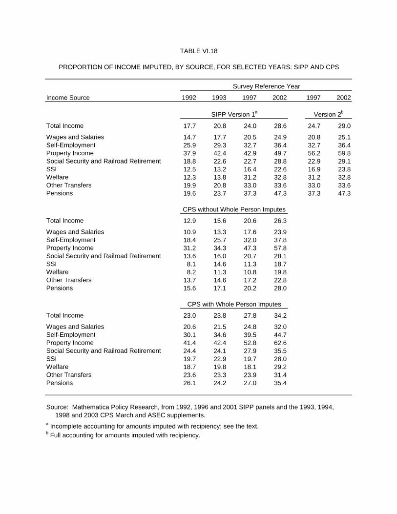
TABLE VI.18

PROPORTION OF INCOME IMPUTED, BY SOURCE, FOR SELECTED YEARS: SIPP AND CPS

Survey Reference Year

Income Source 1992 1993 1997 2002 1997 2002

SIPP Version 1a Version 2b

Total Income 17.7 20.8 24.0 28.6 24.7 29.0

Wages and Salaries 14.7 17.7 20.5 24.9 20.8 25.1Self-Employment 25.9 29.3 32.7 36.4 32.7 36.4Property Income 37.9 42.4 42.9 49.7 56.2 59.8Social Security and Railroad Retirement 18.8 22.6 22.7 28.8 22.9 29.1SSI 12.5 13.2 16.4 22.6 16.9 23.8Welfare 12.3 13.8 31.2 32.8 31.2 32.8Other Transfers 19.9 20.8 33.0 33.6 33.0 33.6Pensions 19.6 23.7 37.3 47.3 37.3 47.3

CPS without Whole Person Imputes

Total Income 12.9 15.6 20.6 26.3

Wages and Salaries 10.9 13.3 17.6 23.9Self-Employment 18.4 25.7 32.0 37.8Property Income 31.2 34.3 47.3 57.8Social Security and Railroad Retirement 13.6 16.0 20.7 28.1SSI 8.1 14.6 11.3 18.7Welfare 8.2 11.3 10.8 19.8Other Transfers 13.7 14.6 17.2 22.8Pensions 15.6 17.1 20.2 28.0

CPS with Whole Person Imputes

Total Income 23.0 23.8 27.8 34.2

Wages and Salaries 20.6 21.5 24.8 32.0Self-Employment 30.1 34.6 39.5 44.7Property Income 41.4 42.4 52.8 62.6Social Security and Railroad Retirement 24.4 24.1 27.9 35.5SSI 19.7 22.9 19.7 28.0Welfare 18.7 19.8 18.1 29.2Other Transfers 23.6 23.3 23.9 31.4Pensions 26.1 24.2 27.0 35.4

Source: Mathematica Policy Research, from 1992, 1996 and 2001 SIPP panels and the 1993, 1994, 1998 and 2003 CPS March and ASEC supplements.a Incomplete accounting for amounts imputed with recipiency; see the text.b Full accounting for amounts imputed with recipiency.

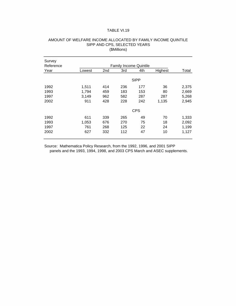
TABLE VI.19

AMOUNT OF WELFARE INCOME ALLOCATED BY FAMILY INCOME QUINTILESIPP AND CPS, SELECTED YEARS

($Millions)

SurveyReference Family Income QuintileYear Lowest 2nd 3rd 4th Highest Total

SIPP

1992 1,511 414 236 177 36 2,3751993 1,794 459 183 153 80 2,6691997 3,149 962 582 287 287 5,2682002 911 428 228 242 1,135 2,945

CPS

1992 611 339 265 49 70 1,3331993 1,053 676 270 75 18 2,0921997 761 268 125 22 24 1,1992002 627 332 112 47 10 1,127

Source: Mathematica Policy Research, from the 1992, 1996, and 2001 SIPP panels and the 1993, 1994, 1998, and 2003 CPS March and ASEC supplements.

TABLE VI.20

DISTRIBUTION OF SIPP IMPUTED INCOME BY FAMILY INCOME QUINTILE:SELECTED SOURCES OF INCOME BY YEAR

SurveyReference Family Income QuintileYear Lowest 2nd 3rd 4th Highest Total

Welfare1992 63.6 17.4 9.9 7.5 1.5 100.01993 67.2 17.2 6.8 5.7 3.0 100.01997 59.8 18.3 11.0 5.5 5.4 100.02002 31.0 14.5 7.7 8.2 38.5 100.0

SSI1992 60.1 14.5 8.3 12.6 4.5 100.01993 55.9 18.9 10.1 9.2 5.9 100.01997 36.4 27.0 16.1 12.2 8.3 100.02002 39.7 25.1 17.5 11.4 6.3 100.0

Pensions1992 6.6 21.9 22.6 25.6 23.3 100.01993 6.4 21.7 23.4 24.4 24.1 100.01997 7.2 19.5 24.1 23.8 25.4 100.02002 6.9 18.2 24.1 26.0 24.8 100.0

Other Transfers1992 17.8 19.8 23.9 18.2 20.3 100.01993 19.5 19.8 19.1 19.9 21.5 100.01997 12.7 21.6 16.3 19.6 29.8 100.02002 15.5 18.4 23.2 20.2 22.7 100.0

Social Security and Railroad Retirement1992 27.2 30.7 17.4 14.8 9.9 100.01993 25.7 30.2 19.7 15.1 9.3 100.01997 28.0 30.8 19.7 13.3 8.2 100.02002 24.4 28.7 22.1 14.7 10.1 100.0

Wages and Salaries1992 4.0 11.5 18.9 24.3 41.3 100.01993 4.4 12.7 17.8 25.5 39.6 100.01997 4.4 11.6 17.2 25.0 41.8 100.02002 4.5 11.0 16.7 25.1 42.7 100.0

Total Income1992 6.7 13.1 17.5 22.0 40.7 100.01993 6.8 13.8 17.2 22.6 39.5 100.01997 6.6 13.4 16.9 22.5 40.5 100.02002 6.4 13.0 17.4 23.1 40.2 100.0

Source: Mathematica Policy Research, from the 1992, 1996 and 2001 SIPP panels.

FIGURE VI.1 SIPP MONTHLY AND ANNUAL POVERTY RATES VERSUS CPS ANNUAL POVERTY RATES, 1992 THROUGH 2004

0.0

2.0

4.0

6.0

8.0

10.0

12.0

14.0

16.0

18.0

Jan9

2

Jun9

2

Nov

92

Apr

93

Sep

93

Feb

94

Jul9

4

Dec

94

May

95

Oct

95

Mar

96

Aug

96

Jan9

7

Jun9

7

Nov

97

Apr

98

Sep

98

Feb

99

Jul9

9

Dec

99

May

00

Oct

00

Mar

01

Aug

01

Jan0

2

Jun0

2

Nov

02

Apr

03

Sep

03

Feb

04

Jul0

4

Dec

04

Pov

erty

Rat

e

SIPP Monthly

CPS Annual

SIPP Annual

1992 Panel 1996 Panel 2001 Panel 2004 Panel

FIGURE VI.2 SIPP MONTHLY AND ANNUAL POVERTY RATES VERSUS CPS ANNUAL POVERTY RATES, 1992 THROUGH 2004, CHILDREN UNDER 18

0.0

5.0

10.0

15.0

20.0

25.0

30.0

Jan9

2

Jun9

2

Nov

92

Apr

93

Sep

93

Feb

94

Jul9

4

Dec

94

May

95

Oct

95

Mar

96

Aug

96

Jan9

7

Jun9

7

Nov

97

Apr

98

Sep

98

Feb

99

Jul9

9

Dec

99

May

00

Oct

00

Mar

01

Aug

01

Jan0

2

Jun0

2

Nov

02

Apr

03

Sep

03

Feb

04

Jul0

4

Dec

04

Pov

erty

Rat

e

SIPP MonthlyCPS AnnualSIPP Annual

FIGURE VI.3 SIPP MONTHLY AND ANNUAL POVERTY RATES VERSUS CPS ANNUAL POVERTY RATES, 1992 THROUGH 2004, ADULTS 18 TO 24

0.0

5.0

10.0

15.0

20.0

25.0

Jan9

2

Jun9

2

Nov

92

Apr

93

Sep

93

Feb

94

Jul9

4

Dec

94

May

95

Oct

95

Mar

96

Aug

96

Jan9

7

Jun9

7

Nov

97

Apr

98

Sep

98

Feb

99

Jul9

9

Dec

99

May

00

Oct

00

Mar

01

Aug

01

Jan0

2

Jun0

2

Nov

02

Apr

03

Sep

03

Feb

04

Jul0

4

Dec

04

Pov

erty

Rat

e

SIPP MonthlyCPS AnnualSIPP Annual

FIGURE VI.4 SIPP MONTHLY AND ANNUAL POVERTY RATES VERSUS CPS ANNUAL POVERTY RATES, 1992 THROUGH 2004, ADULTS 25 TO 39

0.0

2.0

4.0

6.0

8.0

10.0

12.0

14.0

16.0

18.0

Jan9

2

Jun9

2

Nov

92

Apr

93

Sep

93

Feb

94

Jul9

4

Dec

94

May

95

Oct

95

Mar

96

Aug

96

Jan9

7

Jun9

7

Nov

97

Apr

98

Sep

98

Feb

99

Jul9

9

Dec

99

May

00

Oct

00

Mar

01

Aug

01

Jan0

2

Jun0

2

Nov

02

Apr

03

Sep

03

Feb

04

Jul0

4

Dec

04

Pov

erty

Rat

e

SIPP MonthlyCPS AnnualSIPP Annual

FIGURE VI.5 SIPP MONTHLY AND ANNUAL POVERTY RATES VERSUS CPS ANNUAL POVERTY RATES, 1992 THROUGH 2004, ADULTS 40 TO 64

0.0

2.0

4.0

6.0

8.0

10.0

12.0

14.0

Jan9

2

Jun9

2

Nov

92

Apr

93

Sep

93

Feb

94

Jul9

4

Dec

94

May

95

Oct

95

Mar

96

Aug

96

Jan9

7

Jun9

7

Nov

97

Apr

98

Sep

98

Feb

99

Jul9

9

Dec

99

May

00

Oct

00

Mar

01

Aug

01

Jan0

2

Jun0

2

Nov

02

Apr

03

Sep

03

Feb

04

Jul0

4

Dec

04

Pov

erty

Rat

e

SIPP MonthlyCPS AnnualSIPP Annual

FIGURE VI.6 SIPP MONTHLY AND ANNUAL POVERTY RATES VERSUS CPS ANNUAL POVERTY RATES, 1992 THROUGH 2004, ADULTS 65 AND OLDER

0.0

2.0

4.0

6.0

8.0

10.0

12.0

14.0

Jan9

2

Jun9

2

Nov

92

Apr

93

Sep

93

Feb

94

Jul9

4

Dec

94

May

95

Oct

95

Mar

96

Aug

96

Jan9

7

Jun9

7

Nov

97

Apr

98

Sep

98

Feb

99

Jul9

9

Dec

99

May

00

Oct

00

Mar

01

Aug

01

Jan0

2

Jun0

2

Nov

02

Apr

03

Sep

03

Feb

04

Jul0

4

Dec

04

Pov

erty

Rat

e

SIPP MonthlyCPS AnnualSIPP Annual

233

VII. CONCLUSION AND RECOMMENDATIONS

The principal findings from this evaluation of sample loss in the SIPP and CPS can be

summarized succinctly. Basically, we find no evidence that attrition bias or match bias in the

linking of administrative records to survey data has increased in the SIPP since the 1996 panel.

Furthermore, we find that the Census Bureau’s non-interview adjustment is highly effective in

controlling attrition bias in the SIPP’s longitudinal weights, and we find that by replicating the

Census Bureau’s SIPP and CPS calibration adjustments we can largely eliminate match bias

from matched samples of records obtained from both surveys. Our recommendation to

prospective users of SIPP data at SSA is that they should not hesitate to use the 2001 SIPP panel

any more than they would hesitate to use the 1996 panel. Neither attrition bias nor match bias

provides any more reason to avoid the 2001 panel than the earlier panel.

That being said, however, there are other issues that SIPP users need to understand when

using the data from 1996 and later panels. One, there seems to have emerged a “wave 1 effect”

that elevates poverty rates and possibly other indicators during the first wave of each new panel.

The result is a distortion of trends both within and across panels and an exaggeration of gross

change among panel members between the first and second waves. Two, the new entrants to the

population who are largely unrepresented in a SIPP panel over time could be a major source of

discontinuity in SIPP estimates of poverty and other characteristics between the end of one SIPP

panel and the beginning of the next panel. Third, SIPP estimates of aggregate income showed a

decline relative to independent benchmarks from the initial SIPP panel in 1984 through the mid-

1990s. SIPP estimates of aggregate income have continued to decline relative to the CPS, but

without independent benchmarks after 1996 we cannot determine how much of this relative

decline is due to CPS gains versus SIPP losses. The decline relative to the CPS is particularly

234

striking in the bottom income quintile, where the SIPP captured 20 percent more income than the

CPS in 1993 but only 6 percent more than the CPS in 2002. The SIPP has continued to identify

more sources of income, however, and this is especially true among the elderly. The seeming

paradox of capturing more sources but less total income remains unexplained. For all of these

reasons, SIPP users need to understand the comparative strengths and weaknesses of the SIPP

and the CPS and tailor their uses of the two surveys accordingly.

While we did not find it necessary to develop complex adjustment methodologies to reduce

attrition bias and match bias to acceptable levels, we do recommend that SSA analysts make use

of the calibration procedures that we applied to reweight matched subsamples of SIPP and CPS

records to agree with full sample population totals by selected demographic characteristics.

These procedures are documented in Appendix A and utilize programs that are stored on a

personal computer at SSA.1 We recommend that SSA analysts apply the calibration procedures

to their matched samples before applying any additional controls to meet program administrative

totals. This will ensure that the matched data receive the benefits of a detailed demographic

calibration while still reproducing program administrative controls. In applications to CPS data,

the SSA analysts may want to consider further restricting the matched sample to respondents

who completed the supplement—that is, excluding the whole person imputes discussed in

Chapters II and III.

An issue that arose in SSA’s use of matched data from the 2001 SIPP panel was whether to

restrict the analytical sample to matched records, as had been done with the 1996 panel, or

whether to compensate for the reduced match rate and the potentially greater match bias by

including both matched and unmatched records in the analytic sample. Our findings with respect

1 There are separate programs for calibrating SIPP and CPS matched samples, as the Census Bureau’s

calibration procedures—and the demographic controls that they employ—differ between the two surveys.

235

to match bias support restricting the analytic sample to just the matched records, as there appears

to be no additional bias—after calibration—as a result of the reduced match rate. Restricting the

analytic sample to matched cases allows the SSA analysts to use Social Security program data in

place of survey data for all Social Security beneficiaries in the analytic sample.

The Census Bureau has addressed the declining match rates between survey and

administrative records by developing a probabilistic record linkage methodology that can be

applied to link survey respondents to their SSNs, which then allows the survey records to be

linked to other SSN-based administrative records. With this new methodology it is no longer

necessary to ask survey respondents for their SSNs, and we understand that, as a result, very few

survey respondents are refusing to give their consent to linkages between their survey data and

their administrative records. There is a reasonable expectation that match rates may approach 90

percent again after having fallen into the 70s in the CPS and to 60 percent in the SIPP.

Match errors based on the new methodology are likely to be higher than match errors based

on SSNs because the new approach uses a probabilistic record-linkage approach rather an exact

match. As matched data using the new methodology become available, SSA should plan to

conduct analyses of match quality and devise methods to identify bad matches using the

information provided by comparisons between the survey and administrative reports of Social

Security beneficiary status. In addition, based on what we see for children, it may turn out that

the income differential in match rates among adults is increased when probabilistic matching is

extended to that population. For this reason we would encourage SSA to re-estimate Table II.6

when matched data from the March 2006 CPS become available. More generally, the new

methodology may introduce new forms of match bias that users need to understand. As a

prominent user of matched data, SSA should take the lead in undertaking an evaluation of match

bias with the new methods.

236

The major findings presented in this report would have to be characterized as surprising.

They run counter to what was expected, and they suggest that there are significant

misconceptions about the SIPP. With the Census Bureau undertaking a complete re-engineering

of the SIPP, this report is especially timely. It is critically important that the Census Bureau and

SIPP users who might be moved to influence the design of the new SIPP understand the current

survey’s strengths and limitations, or the re-engineering effort will not achieve all that it could

achieve. Indeed, if the re-engineering focuses on the wrong features, the new survey could prove

to be decidedly inferior to the current survey.

Two areas of concern stand out. The first is the wave 1 effect that we documented in

Chapter V. Only the Census Bureau is in a position to explore this further, as the source of the

problem may lie in field operations or the survey processing that occurs after the data have come

in from the field. If the Census Bureau moves to an annual interview in the re-engineered SIPP,

it is critical that the initial interview not reflect the same problem that we are seeing with the

wave 1 SIPP interview.

The second area of concern stems from the divergent trends in elderly poverty portrayed in

the last chapter. The findings presented therein challenge users to reassess their reliance on

either the CPS or the SIPP to measure the material well-being of the elderly either cross-

sectionally or over time. We recommend that ORES encourage the Census Bureau to undertake

an assessment of how these two surveys can present such inconsistent pictures of changes in

elderly poverty over time. Only with a better understanding of the causes of these

inconsistencies can users of either survey feel confidence in the information that they are able to

extract from SIPP or CPS data.

Lastly, to bring these issues to the Census Bureau’s attention in a manner that will increase

the likelihood of the Census Bureau’s giving them adequate attention, we recommend that SSA

237

take the initiative to set up a briefing of Census Bureau staff with responsibility for the SIPP.

The briefing should cover the major findings from this report but with a particular focus on those

findings that carry the most important implications for the re-engineering of the SIPP.

238

239

REFERENCES

Cody, Scott, Laura Castner, James Mabli, and Julie Sykes. “Dynamics of Food Stamp Program Participation, 2001-2003.” Draft report. Washington, DC: Mathematica Policy Research, Inc., January 2007.

Czajka, John L. “Sample Loss from Attrition in the SIPP.” MPR Memorandum to Jim Sears,

May 4, 2006. Czajka, John L. and Julie Sykes. “Health Insurance Coverage Dynamics among Children and

Nonelderly Adults, 1996-1999.” Washington, DC: Mathematica Policy Research, Inc., October 2006.

Czajka, John L., Jonathan E. Jacobson and Scott Cody. “Survey Estimates of Wealth: A

Comparative Analysis and Review of the Survey of Income and Program Participation.” Washington, DC: Mathematica Policy Research, Inc., August 2003.

Davern, Michael, Holly Rodin, Kathleen Thiede Call and Lynn A. Blewett. “Are the CPS

Uninsurance Estimates Too High? An Examination of Imputation.” Health Services Research, vol. 42, no. 5, 2007, pp. 2038-2055.

Eargle, Judith H. “Sample Loss Rates through Wave 9 for the 2001 Panel.” Memorandum for

the SIPP Record 2004-01. Washington, DC: U.S. Census Bureau, March 2, 2004. Hall, David, Smanchai Sae-Ung, and Jan Tin. “Earned Income and Longitudinal Attrition in the

SIPP and SPD.” Proceedings of the Survey Research Methods Section. Alexandria, VA: American Statistical Association, 2004.

Huynh, Minh, Kalman Rupp, and James Sears. “The Assessment of Survey of Income and

Program Participation (SIPP) Benefit Data Using Longitudinal Administrative Records.” Proceedings of the FCSM Research Conference. Washington: Federal Committee on Statistical Methodology, 2001.

Koenig, Melissa L. “An Assessment of the Current Population Survey and the Survey of Income

and Program Participation Using Social Security Administrative Data.” Proceedings of the FCSM Research Conference. Washington: Federal Committee on Statistical Methodology, 2003.

Passel, Jeffrey S. “The Size and Characteristics of the Unauthorized Migrant Population in the

U.S.: Estimates Based on the March 2005 Current Population Survey.” Research Report. Washington, DC: Pew Hispanic Center, March 2006.

Roemer, Marc I. “Using Administrative Earnings Records to Assess Wage Data Quality in the

March Current Population Survey and the Survey of Income and Program Participation.” Longitudinal Employer-Household Dynamics Technical Paper No. TP-2002-22. Washington, DC: U.S. Census Bureau, November 2002.

240

Roemer, Marc I. “Assessing the Quality of the March Current Population Survey and the Survey

of Income and Program Participation Income Estimates, 1990-1996.” Working Paper, Housing and Household Economic Statistics Division. Washington, DC: U.S. Census Bureau, June 2000.

Rosenbach, Margo, et al. “National Evaluation of the State Children’s Health Insurance

Program: A Decade of Expanding Coverage and Improving Access.” Final Report. Washington, DC: Mathematica Policy Research, September 2007.

Sears, James and Kalman Rupp. “Exploring Social Security Payment History Matched with the

Survey of Income and Program Participation.” Proceedings of the FCSM Research Conference. Washington: Federal Committee on Statistical Methodology, 2003.

Toder, Eric, et al. “Modeling Income in the Near Term: Revised Projections of Retirement

Income Through 2020 for the 1931-1960 Birth Cohorts.” Washington, DC: The Urban Institute, June 2002.

U.S. Census Bureau. Current Population Survey, 2003 ASEC Technical Documentation.

Washington, DC: U.S. Department of Commerce, November 2003. U.S. Census Bureau. “Current Population Survey Technical Paper 63RV: Design and

Methodology.” Washington, DC: U.S. Department of Commerce, March 2002. U.S. Census Bureau. Survey of Income and Program Participation Users’ Guide. Third Edition.

Washington, DC: U.S. Census Bureau, 2001. U.S. Census Bureau. Current Population Reports, Series P-70, No. 24. “Transitions in Income

and Poverty Status: 1987-88.” Washington, DC: U.S. Government Printing Office, 1991. Vaughan, Denton R. “Reflections on the Income Estimates from the Initial Panel of the Survey

of Income and Program Participation (SIPP).” Studies in Income Distribution No. 17. Washington, DC: Social Security Administration, May 1993.

Vaughan, Denton, and Fritz Scheuren. “Longitudinal Attrition in SIPP and SPD.” Proceedings

of the Social Statistics Section. Alexandria, VA: American Statistical Association, 2002. Weinberg, Daniel H. “Using the Survey of Income and Program Participation for Policy

Analysis.” SIPP Working Paper No. 240. Washington, DC: U.S. Census Bureau, 2003.

A-1

APPENDIX A

CALIBRATION OF SAMPLES

A-3

CALIBRATION OF SAMPLES

A. INTRODUCTION The weights that are assigned to matched samples of survey and administrative records (and, for the CPS, the subset of sample members who responded to the annual supplement and, therefore, did not have to have all of their supplement variables imputed) must be calibrated so that they sum to the same population control totals as the corresponding full sample weights. Calibration adjusts each matched sample to compensate for differential match rates by sex, age, race and ethnicity (and, for the CPS, by state of residence as well).

We created these calibrated samples:

1. Matched full panel sample for 1996 and 2001

2. Matched calendar-year samples for 1996, 1997, 1998, 2001, and 2002

3. Matched core-wave samples for March 1996 (wave 1), July 1996 (wave 2), November 1996 (wave 3), November 1997 (wave 6), November 1998 (wave 9), May 2001 (wave 2), September 2001 (wave 3), September 2002 (wave 6), and September 2003 (wave 9)

4. Wave 1/wave 2 sample (i.e. present in common month of wave 1 and present all 4 months of wave 2) for 1996 and 2001

5. Matched wave 1/wave 2 sample (i.e. present in common month of wave 1 and present all 4 months of wave 2) for 1996 and 2001

6. CPS supplemental sample (i.e. persons with FL_665 = 1) for 1996, 1997, 2001, 2002, and 2003

7. Matched CPS full sample for 1996, 1997, 2001, 2002, and 2003

8. Matched CPS supplemental sample for 1996, 1997, 2001, 2002, and 2003

For each SIPP sample we calibrated the sample weight and the 108 replicate weights that are associated with the sample weight. Calibration of the replicate weights is necessary if they are to be used in conjunction with the calibrated sample weight to calculate standard errors. Table A.1 lists the SIPP and CPS sample weights that we calibrated and, for the SIPP, the replicate weights that we calibrated along with the sample weights. B. CALIBRATION METHODOLOGY Our calibration procedures were designed to replicate the final stage in the Census Bureau’s calculation of sample weights and replicate weights for the SIPP and sample weights for the CPS March or ASEC supplement. Calibration adjusts the sample weights by the application of “raking” (alternating ratio—or multiplicative—adjustments) so that they sum to a cross-classification of the survey universe by a set of demographic characteristics. For the SIPP, the

A-4

calibration matrix also includes the survey rotation group. Tables A.2 through A.6 show the potential calibration cells (prior to collapsing, discussed below) for the SIPP calibration. Table A.2 shows the potential calibration cells for Hispanic children and adults. (Note that Hispanic children are raked with all children while Hispanic adults are raked with adult males and adult females.) Table A.3 shows the potential calibration cells for children 15 by race, sex, and age. Table A.4 shows the potential calibration cells for adult females by race and age, and Table A.5 shows the same for adult males. Lastly, Table A.6 shows the potential calibration cells for the household relationship code by race and sex. Through calibration, the weights are adjusted so that they satisfy all of the applicable control totals. For example, for nonblack females the applicable control totals would be found in tabulations corresponding to Tables A.4 and A.6 while the control totals for all adult females broken down by Hispanic versus non-Hispanic would be found in the tabulation corresponding to Table A.2. The raking algorithm is iterative. Raking programs can be set up to run for a fixed number of iterations, or they can be devised to run to convergence—that is, until the control totals are fit to within a specified tolerance. We opted to write our programs to run for a fixed number of iterations. The number of iterations is parameterized. This parameter is currently set to 10. We have found that 10 iterations are sufficient to match the control totals to within one or two persons (with most of the deviations being zero). If there is an inconsistency in the control totals—for example, if one set of matrices yields a different total number of persons than another set—the raking algorithm will not converge. Therefore, it is advisable to check the specified controls for internal inconsistencies before running the calibration program. The calibration programs re-estimate the control matrices with the calibrated weights and calculate differences between these matrices and the control matrices. The user should check that these differences are predominantly zero and never exceed 2 (or an alternative acceptable maximum). The SIPP calibration matrices include more detailed age groups than the sample may be able to support—even with all of the observations. Therefore, it is necessary for the user to review a tabulation of weighted sample records by the calibration matrices in order to determine if the Census Bureau used all of the possible age detail in calibrating the full sample weights or if some collapsing was done.1 The Census Bureau rakes the SIPP weights to convergence, so it is easy to determine what control totals were used to calibrate a given sample weight. The subtotals for a given age group or household relationship code within race and sex will be identical across the four rotation groups if that age group was used without collapsing. Table A.7 shows the original calibration tabulation for adult black males for wave 2 of the 2001 SIPP panel and, in the bottom panel of the table, the collapsing of age groups that was necessary to achieve identical sums across the four rotation groups. If the matched subsample represents much less than 90 percent of the full population that corresponds to a given sample weight, some additional collapsing of age groups or relationship codes beyond may be desirable to avoid excessive weight adjustments. After establishing how the Census Bureau collapsed the age groups and relationship codes, the user may want to examine the sample sizes and preliminary weighted totals obtained when the matched subsample 1 The household relationship codes may have been collapsed as well. These must be examined separately.

A-5

is distributed across the control matrices. Some of the programs listed in the next section can be used to produce such tabulations. C. IMPLEMENTATION OF THE CALIBRATION METHODOLOGY Calibration of the SIPP weights requires several steps. The first step is to extract the control variables and cross-sectional weights from the SIPP core-wave files and obtain the full panel and calendar year weights from the longitudinal weight file. If replicate weights are to be calibrated as well, they must be extracted from files provided by the Census Bureau, converted to SAS, and renamed.2 A pair of tabulation programs is then run to produce preliminary control totals, which are written to Excel spreadsheets (for example, calibration_wave01_1996_wpfinwgt.xls) named with the wave and panel and type of weight. These tabulations must be reviewed to determine if the Census Bureau performed any collapsing across age or relationship to the householder. The user can examine the following files that are produced by the tabulation programs listed later in this section: Calibration_waveWAVE_PANEL_WGT.xls Calibration_cyYEAR_WGT.xls HR-code_cyYEAR_WGT.xls HR-code_waveWAVE_PANEL_WGT.xls Match_Calibration_waveWAVE_PANEL_WGT.xls Match_Calibration_cyYEAR_WGT.xls Match_HR-code_cyYEAR_WGT.xls Match_HR-code_waveWAVE_PANEL_WGT.xls Where WAVE is the wave number (for example, 01), PANEL is the SIPP panel (for example, 2001), YEAR is the calendar year within the panel (for example, 2002), and WGT is the name of the weight variable used. The user may also want to consider additional collapsing to improve the statistical properties of the calibrated weights.3 Ultimately, the user determines whether or not to manually collapse some of the rows in the preliminary control totals in order to obtain final control totals. The final control totals are then copied into a set of Excel worksheets that are used by the calibration programs. Three Excel files contain the full set of controls for a given SIPP weight. 2 The replicate weights are not posted to a Census Bureau website. They must be requested from the Demographic Statistical Methods Division. The names assigned to the replicate weights are not standardized, so Table A.1 does not list the original variable names. 3 In addition to ensuring that the collapsed control totals produce identical cell counts across rotation groups, one could collapse even further to reduce the variability of the calibrated weights. Programs that tabulate various matched subsamples can be used to obtain weighted and unweighted sample tabulations that are useful for such analysis. For example, if some of the cells end up with much smaller sample counts than other cells in the same row, one could collapse across rows to make the cell counts more nearly equal. We did not do this because we were concerned that using less detailed controls for the matched subsample versus the full sample would contribute to estimated match bias. In an application of matched data to a research problem, however, there might be reason to prefer less variable weights in order to improve the precision of estimates from the matched subsample.

A-6

For example, the controls used to calibrate the wave 1 sample from the 2001 SIPP panel are found in: Calibration_controls_for_adults_2001_wave01_A.xls Calibration_controls_for_kids_2001_wave01_A.xls HR-code_controls_2001_wave01_A.xls Here the “A” differentiates the most detailed set of wave 1 controls from a less detailed set of January 2001 controls that might be used to calibrate the full panel sample. Less detailed controls may be required when calibration is used to compensate for substantial sample loss, as with a full panel sample or the extent of nonmatching that occurred with the 2001 SIPP panel. Replicate weights are calibrated in the same set of programs as the sample weights to which they correspond. If replicate weights are to be calibrated along with the sample weight, then “_repwgts” is appended to the name of the calibration control file, as in: Calibration_controls_for_adults_2001_wave01_A_repwgts.xls Calibration_controls_for_kids_2001_wave01_A_repwgts.xls HR-code_controls_2001_wave01_A_repwgts.xls There is no difference in the contents of the control files—just their names. Likewise, except for a small quality assurance step described below, the only difference in the output is that 109 rather than just one set of adjusted weights will be written to an output file. Tables designed to confirm that the calibrated sample weight matches the control totals are not repeated for the replicate weights, as the calibration procedure applied to the sample weights is simply repeated for each of the 108 sets of replicate weights. Depending on the weight that is being calibrated, the user then selects one of five sets of calibration programs to read the collapsed version of the control totals and calibrate the sample weight—and corresponding replicate weights if they are being calibrated as well. The calibration method for adults (persons 15 and older) differs from that for children. Therefore, one program calibrates the weights for adults; another calibrates the weights for children; and a third program combines the two sets of weights and renames them. Each of the two calibration programs also tabulates the calibrated sample weights and writes the calibrated estimates to a separate set of worksheets in the control totals Excel file. These worksheets have “(2)” in the name. As a quality assurance check, to ensure that we iterated enough times in the calibration, each program subtracts the final calibrated estimates from the control totals and writes the differences into worksheets with “(3)” in the name.4 The third program also performs a simple quality control check of the calibrated replicate weights. Sums of the 1st, 50th, and 108th calibrated replicate weights are written to a file, which the user can manually inspect to ensure that these sums are identical to each other and to the sum of the calibrated sample weight. Given that the same methodology is applied to calibrate all 109 weights, these totals require only a cursory review.

4 In our applications, all totals based on the calibrated weights were the same or very close to the control totals.

A-7

The specific programs are as follows:5

A. Extract Data from SIPP

XT_PM.SAS

B. Make Replicate weights from Census Bureau files

1. MK_REPWGTS_FOR_1996_LGTPNLWT.SAS

2. MK_REPWGTS_FOR_2001_LGTPNLWT.SAS

3. MK_REPWGTS_LGTCYWT.SAS

4. MK_REPWGTS_WPFINWGT.SAS

C. Extract Data from SIPP

XT_PM.SAS

D. Make Replicate weights from Census Bureau files

1. MK_REPWGTS_FOR_1996_LGTPNLWT.SAS

2. MK_REPWGTS_FOR_2001_LGTPNLWT.SAS

3. MK_REPWGTS_LGTCYWT.SAS

4. MK_REPWGTS_WPFINWGT.SAS

E. Tabulate Preliminary Control Totals for Cross-sectional Weights

1. TB_CALIBRATION.SAS

2. TB_HR-CODE.SAS

F. Tabulate Preliminary Control Totals for Calendar Year Weights

1. TB_CY_CALIBRATION.SAS

2. TB_CY_HR-CODE.SAS

5 The programs were designed to be re-used as much as possible. Parameters, located at the beginning of the program, identify the panel, the analysis date, the input files, and the output files.

A-8

G. Tabulate Initial Set of Matched Sample Control Totals

1. TB_MATCH_CALIBRATION.SAS

2. TB_MATCH_HR-CODE.SAS

3. TB_MATCH_CY_CALIBRATION.SAS

4. TB_MATCH_CY_HR-CODE.SAS

H. Calibrate Matched Full Panel Sample (CBFPWGT)

1. CALIBRATE_FP_MATCH_ADULTS_REPWGTS.SAS

2. CALIBRATE_FP_MATCH_KIDS_REPWGTS.SAS

3. MK_CBFPWGT_REPWGTS.SAS

I. Calibrate Matched Calendar-Year Samples for 1996, 1997, 1998, 2001, and 2002 (CBCYWGT)

1. CALIBRATE_CY_MATCH_ADULTS_REPWGTS.SAS

2. CALIBRATE_CY_MATCH_KIDS_REPWGTS.SAS

3. MK_CBCYWGT_REPWGTS.SAS

J. Calibrate Matched Core-Wave Samples for March 1996, July 1996, November 1996, November 1997, November 1998, May 2001, September 2001, September 2002, and September 2003 (CBCWWGT)

1. CALIBRATE_MATCH_ADULTS_REPWGTS.SAS

2. CALIBRATE_MATCH_KIDS_REPWGTS.SAS

3. MK_CBCWWGT_REPWGTS.SAS

K. Calibrate Wave 1-Wave 2 Sample (i.e. present in common month of wave 1 and present all 4 months of wave 2) for 1996 and 2001 (CBW1W2WTA)

1. CALIBRATE_W1W2_ADULTS_REPWGTS.SAS

2. CALIBRATE_W1W2_KIDS_REPWGTS.SAS

3. MK_CBW1W2WT_REPWGTS.SAS

L. Calibrate Matched Wave 1-Wave 2 Sample (i.e. present in common month of wave 1 and present all 4 months of wave 2) for 1996 and 2001 (CBW1W2WTB)

A-9

1. CALIBRATE_MATCH_W1W2_ADULTS_REPWGTS.SAS

2. CALIBRATE_MATCH_W1W2_KIDS_REPWGTS.SAS

3. MK_MATCH_CBW1W2WT_REPWGTS.SAS

Calibration of the CPS does not require either external control totals or external weights, so the calibration of the CPS sample weight for all three subsamples can be accomplished in a single program, CPS_CALIBRATION.SAS. The CPS calibration matrices are documented in Tables A.8 through A.10. There is no provision for collapsing any of the rows in the CPS calibration program. One difference between the CPS and SIPP calibration should be noted, although it has no bearing on the user, as this difference is incorporated into the programs. Both the CPS and the SIPP include roughly 800,000 members of the armed forces who are living with civilian adults (15 and older). These members of the armed forces are excluded from the CPS calibration, meaning that their weights are not adjusted. This can produce small differences between the weighted totals for the matched and full CPS samples. In the SIPP, these members of the armed forces are included in the calibration totals. Their weights are adjusted, so the weighted totals for the matched and full SIPP samples will be identical. D. PREPARATION OF THE CALIBRATION PROGRAMS FOR SSA USE Each of the programs provided to SSA has been documented to direct the user to a list of parameters that must be altered to enable the program to find the appropriate data files and to output the results. Except for the programs used to calibrate the wave 1/wave 2 samples, each of the programs listed above was tested on an SSA machine by an MPR systems analyst who had not participated in their creation but was familiar with SIPP and CPS data. Only the documented changes were necessary, and each program ran without error.

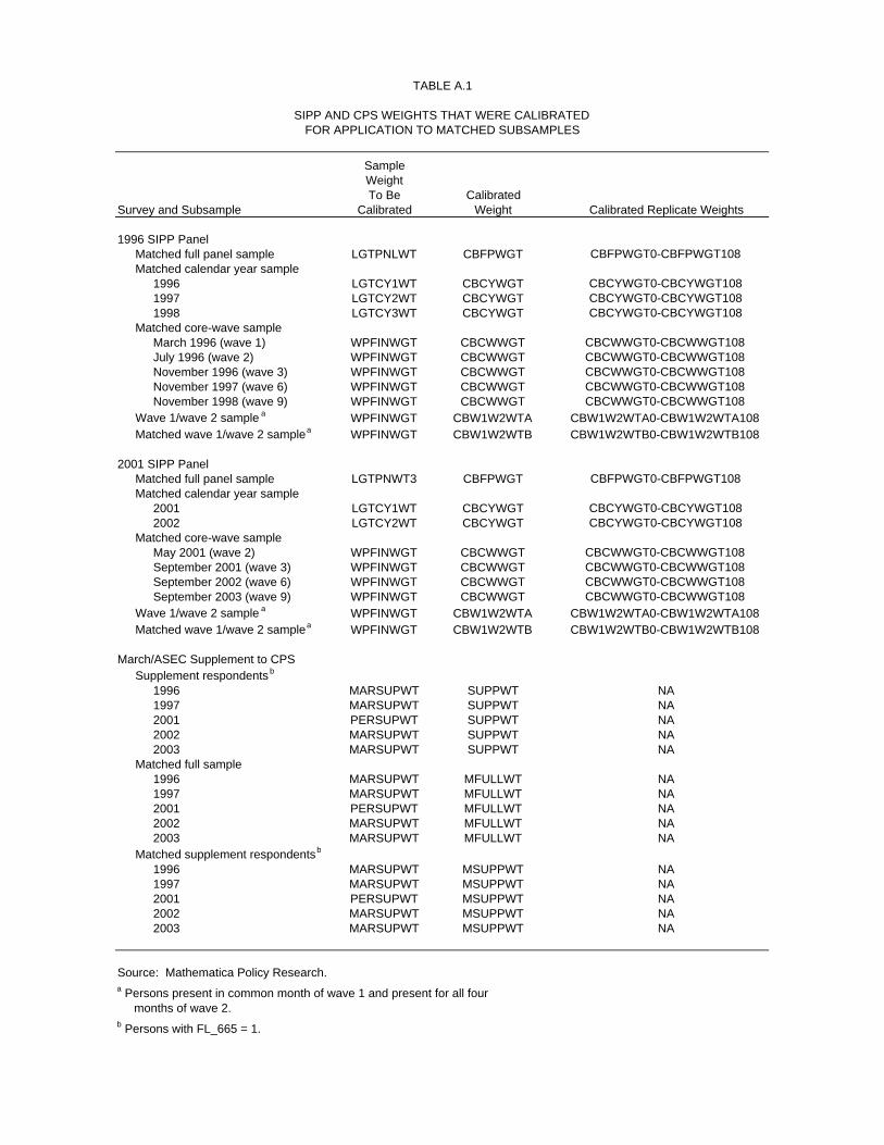
TABLE A.1

SIPP AND CPS WEIGHTS THAT WERE CALIBRATEDFOR APPLICATION TO MATCHED SUBSAMPLES

SampleWeightTo Be Calibrated

Survey and Subsample Calibrated Weight Calibrated Replicate Weights

1996 SIPP PanelMatched full panel sample LGTPNLWT CBFPWGT CBFPWGT0-CBFPWGT108Matched calendar year sample

1996 LGTCY1WT CBCYWGT CBCYWGT0-CBCYWGT1081997 LGTCY2WT CBCYWGT CBCYWGT0-CBCYWGT1081998 LGTCY3WT CBCYWGT CBCYWGT0-CBCYWGT108

Matched core-wave sampleMarch 1996 (wave 1) WPFINWGT CBCWWGT CBCWWGT0-CBCWWGT108July 1996 (wave 2) WPFINWGT CBCWWGT CBCWWGT0-CBCWWGT108November 1996 (wave 3) WPFINWGT CBCWWGT CBCWWGT0-CBCWWGT108November 1997 (wave 6) WPFINWGT CBCWWGT CBCWWGT0-CBCWWGT108November 1998 (wave 9) WPFINWGT CBCWWGT CBCWWGT0-CBCWWGT108

Wave 1/wave 2 sample a WPFINWGT CBW1W2WTA CBW1W2WTA0-CBW1W2WTA108Matched wave 1/wave 2 sample a WPFINWGT CBW1W2WTB CBW1W2WTB0-CBW1W2WTB108

2001 SIPP PanelMatched full panel sample LGTPNWT3 CBFPWGT CBFPWGT0-CBFPWGT108Matched calendar year sample

2001 LGTCY1WT CBCYWGT CBCYWGT0-CBCYWGT1082002 LGTCY2WT CBCYWGT CBCYWGT0-CBCYWGT108

Matched core-wave sampleMay 2001 (wave 2) WPFINWGT CBCWWGT CBCWWGT0-CBCWWGT108September 2001 (wave 3) WPFINWGT CBCWWGT CBCWWGT0-CBCWWGT108September 2002 (wave 6) WPFINWGT CBCWWGT CBCWWGT0-CBCWWGT108September 2003 (wave 9) WPFINWGT CBCWWGT CBCWWGT0-CBCWWGT108

Wave 1/wave 2 sample a WPFINWGT CBW1W2WTA CBW1W2WTA0-CBW1W2WTA108Matched wave 1/wave 2 sample a WPFINWGT CBW1W2WTB CBW1W2WTB0-CBW1W2WTB108

March/ASEC Supplement to CPSSupplement respondents b

1996 MARSUPWT SUPPWT NA1997 MARSUPWT SUPPWT NA2001 PERSUPWT SUPPWT NA2002 MARSUPWT SUPPWT NA2003 MARSUPWT SUPPWT NA

Matched full sample1996 MARSUPWT MFULLWT NA1997 MARSUPWT MFULLWT NA2001 PERSUPWT MFULLWT NA2002 MARSUPWT MFULLWT NA2003 MARSUPWT MFULLWT NA

Matched supplement respondents b

1996 MARSUPWT MSUPPWT NA1997 MARSUPWT MSUPPWT NA2001 PERSUPWT MSUPPWT NA2002 MARSUPWT MSUPPWT NA2003 MARSUPWT MSUPPWT NA

Source: Mathematica Policy Research.a Persons present in common month of wave 1 and present for all four months of wave 2.b Persons with FL_665 = 1.

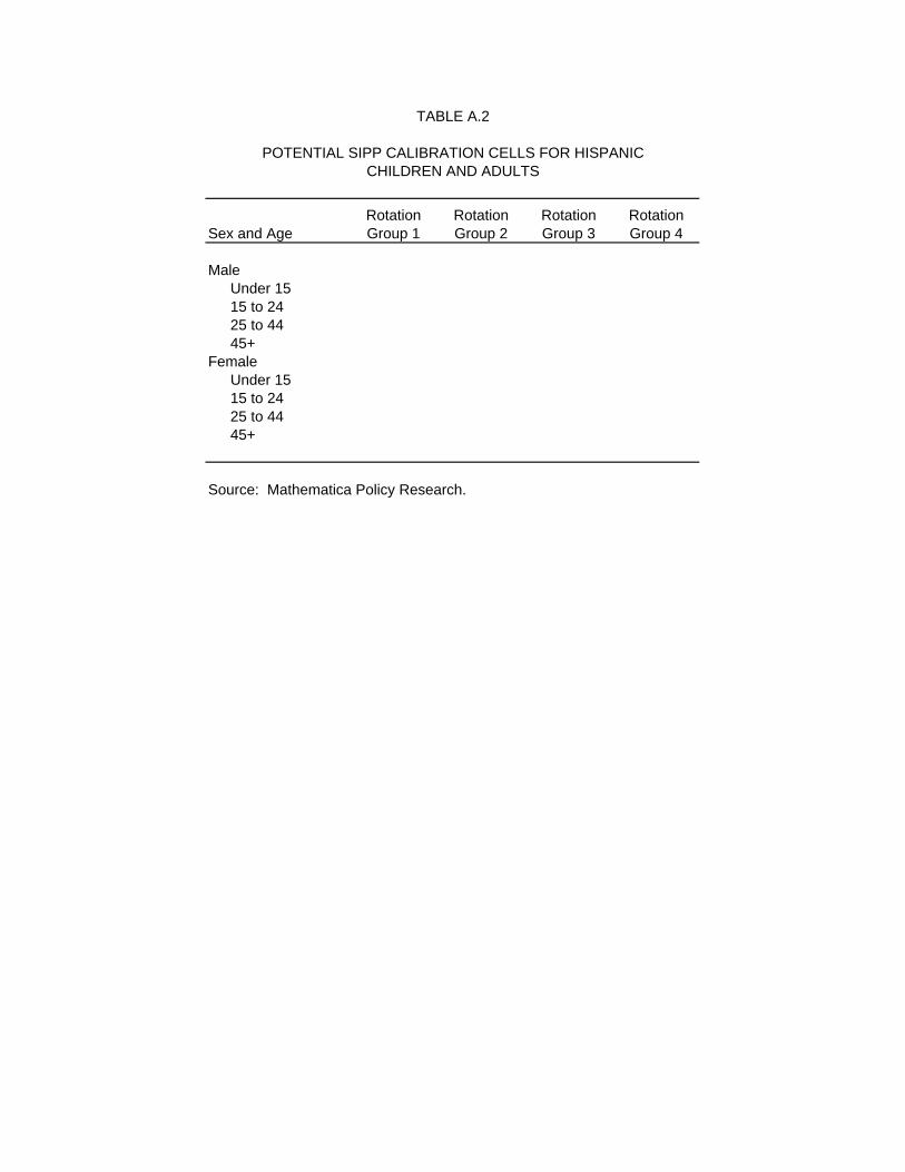
TABLE A.2

POTENTIAL SIPP CALIBRATION CELLS FOR HISPANICCHILDREN AND ADULTS

Rotation Rotation Rotation RotationSex and Age Group 1 Group 2 Group 3 Group 4

MaleUnder 1515 to 2425 to 4445+

FemaleUnder 1515 to 2425 to 4445+

Source: Mathematica Policy Research.

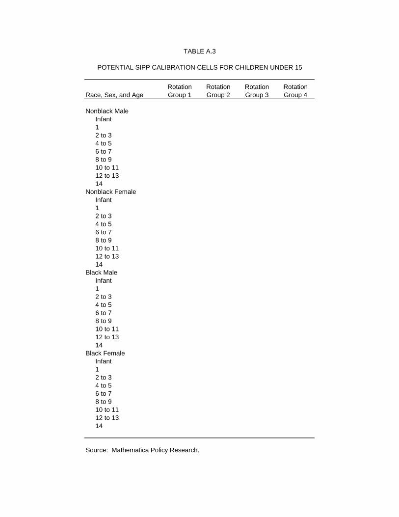
TABLE A.3

POTENTIAL SIPP CALIBRATION CELLS FOR CHILDREN UNDER 15

Rotation Rotation Rotation RotationRace, Sex, and Age Group 1 Group 2 Group 3 Group 4

Nonblack MaleInfant12 to 34 to 56 to 78 to 910 to 1112 to 1314

Nonblack FemaleInfant12 to 34 to 56 to 78 to 910 to 1112 to 1314

Black MaleInfant12 to 34 to 56 to 78 to 910 to 1112 to 1314

Black FemaleInfant12 to 34 to 56 to 78 to 910 to 1112 to 1314

Source: Mathematica Policy Research.

TABLE A.4

POTENTIAL SIPP CALIBRATION CELLS FOR ADULT FEMALES

Rotation Rotation Rotation RotationRace and Age Group 1 Group 2 Group 3 Group 4

Nonblack1516 to 1718 to 1920 to 2122 to 2425 to 2930 to 3435 to 3940 to 4445 to 4950 to 5455 to 5960 to 6162 to 6465 to 6970 to 7475 to 7980 to 8485+

Black1516 to 1718 to 1920 to 2122 to 2425 to 2930 to 3435 to 3940 to 4445 to 4950 to 5455 to 5960 to 6162 to 6465 to 6970 to 7475+

Source: Mathematica Policy Research.

TABLE A.5

POTENTIAL SIPP CALIBRATION CELLS FOR ADULT MALES

Rotation Rotation Rotation RotationRace and Age Group 1 Group 2 Group 3 Group 4

Nonblack1516 to 1718 to 1920 to 2122 to 2425 to 2930 to 3435 to 3940 to 4445 to 4950 to 5455 to 5960 to 6162 to 6465 to 6970 to 7475 to 7980 to 8485+

Black1516 to 1718 to 1920 to 2122 to 2425 to 2930 to 3435 to 3940 to 4445 to 4950 to 5455 to 5960 to 6162 to 6465 to 6970+

Source: Mathematica Policy Research.

TABLE A.6

POTENTIAL SIPP CALIBRATION CELLS FOR RELATIONSHIP CODE, BY RACE AND SEX

Rotation Rotation Rotation RotationRace, Sex, and Relationship Code Group 1 Group 2 Group 3 Group 4

Nonblack FemaleHouseholder with no spouse present but own kidsHouseholder with no spouse present and no kidsHouseholder with spouse presentHouseholder with no relatives presentSpouse of householder or subfamily reference personOther relative of householderNonrelative of householder

Black FemaleHouseholder with no spouse presentHouseholder with spouse presentHouseholder with no relatives presentSpouse of householder or subfamily reference personOther relative of householderNonrelative of householder

Nonblack MaleHouseholder with relatives presentHouseholder with no relatives presentSpouse of householder or subfamily reference personOther relative of householderNonrelative of householder

Black MaleHouseholder with relatives presentHouseholder with no relatives presentSpouse of householder or subfamily reference personOther relative of householderNonrelative of householder

Source: Mathematica Policy Research.

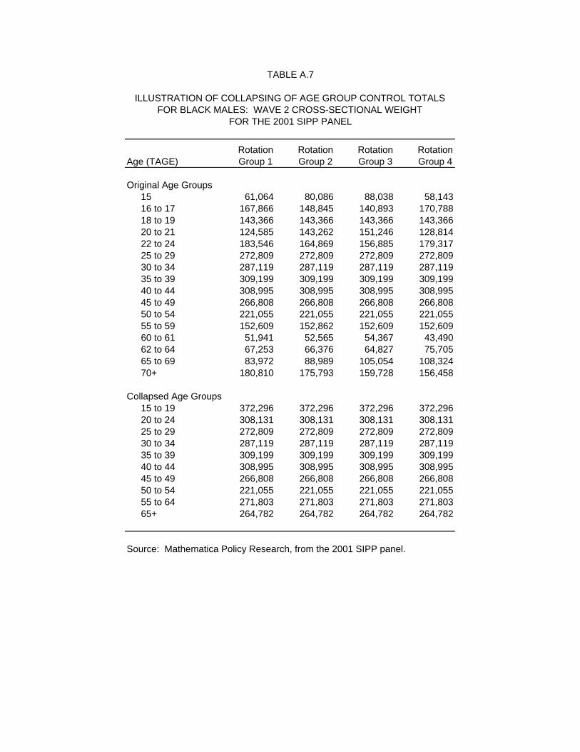
TABLE A.7

ILLUSTRATION OF COLLAPSING OF AGE GROUP CONTROL TOTALSFOR BLACK MALES: WAVE 2 CROSS-SECTIONAL WEIGHT

FOR THE 2001 SIPP PANEL

Rotation Rotation Rotation RotationAge (TAGE) Group 1 Group 2 Group 3 Group 4

Original Age Groups15 61,064 80,086 88,038 58,14316 to 17 167,866 148,845 140,893 170,78818 to 19 143,366 143,366 143,366 143,36620 to 21 124,585 143,262 151,246 128,81422 to 24 183,546 164,869 156,885 179,31725 to 29 272,809 272,809 272,809 272,80930 to 34 287,119 287,119 287,119 287,11935 to 39 309,199 309,199 309,199 309,19940 to 44 308,995 308,995 308,995 308,99545 to 49 266,808 266,808 266,808 266,80850 to 54 221,055 221,055 221,055 221,05555 to 59 152,609 152,862 152,609 152,60960 to 61 51,941 52,565 54,367 43,49062 to 64 67,253 66,376 64,827 75,70565 to 69 83,972 88,989 105,054 108,32470+ 180,810 175,793 159,728 156,458

Collapsed Age Groups15 to 19 372,296 372,296 372,296 372,29620 to 24 308,131 308,131 308,131 308,13125 to 29 272,809 272,809 272,809 272,80930 to 34 287,119 287,119 287,119 287,11935 to 39 309,199 309,199 309,199 309,19940 to 44 308,995 308,995 308,995 308,99545 to 49 266,808 266,808 266,808 266,80850 to 54 221,055 221,055 221,055 221,05555 to 64 271,803 271,803 271,803 271,80365+ 264,782 264,782 264,782 264,782

Source: Mathematica Policy Research, from the 2001 SIPP panel.

TABLE A-8

CPS POPULATION CONTROLS FOR STEP 1:STATE POPULATIONS 16 AND OLDER

CivilianNoninstitutional

PersonsState 16 and Older

AlabamaAlaskaArizonaArkansasCaliforniaColoradoConnecticutDelawareDistrict of ColumbiaFloridaGeorgiaHawaiiIdahoIllinoisIndianaIowaKansasKentuckyLouisianaMaineMarylandMassachusettsMichiganMinnesotaMississippiMissouriMontanaNebraskaNevadaNew HampshireNew JerseyNew MexicoNew YorkNorth CarolinaNorth DakotaOhioOklahomaOregon

Continued

Table A-8 Continued

CivilianNoninstitutional

PersonsState 16 and Older

PennsylvaniaRhode IslandSouth CarolinaSouth DakotaTennesseeTexasUtahVermontVirginiaWashingtonWest VirginiaWisconsinWyoming

Source: Current Population Survey Technical Paper 63RV, Design and Methodology, March 2002, p. 10-5.

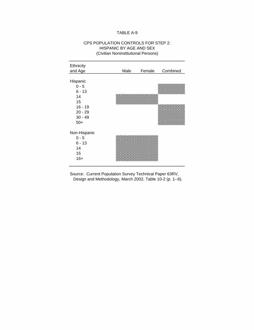
TABLE A-9

CPS POPULATION CONTROLS FOR STEP 2:HISPANIC BY AGE AND SEX

(Civilian Noninstitutional Persons)

Ethnicityand Age Male Female Combined

Hispanic0 - 56 - 13141516 - 1920 - 2930 - 4950+

Non-Hispanic0 - 56 - 13141516+

Source: Current Population Survey Technical Paper 63RV, Design and Methodology, March 2002, Table 10-2 (p. 1--6).

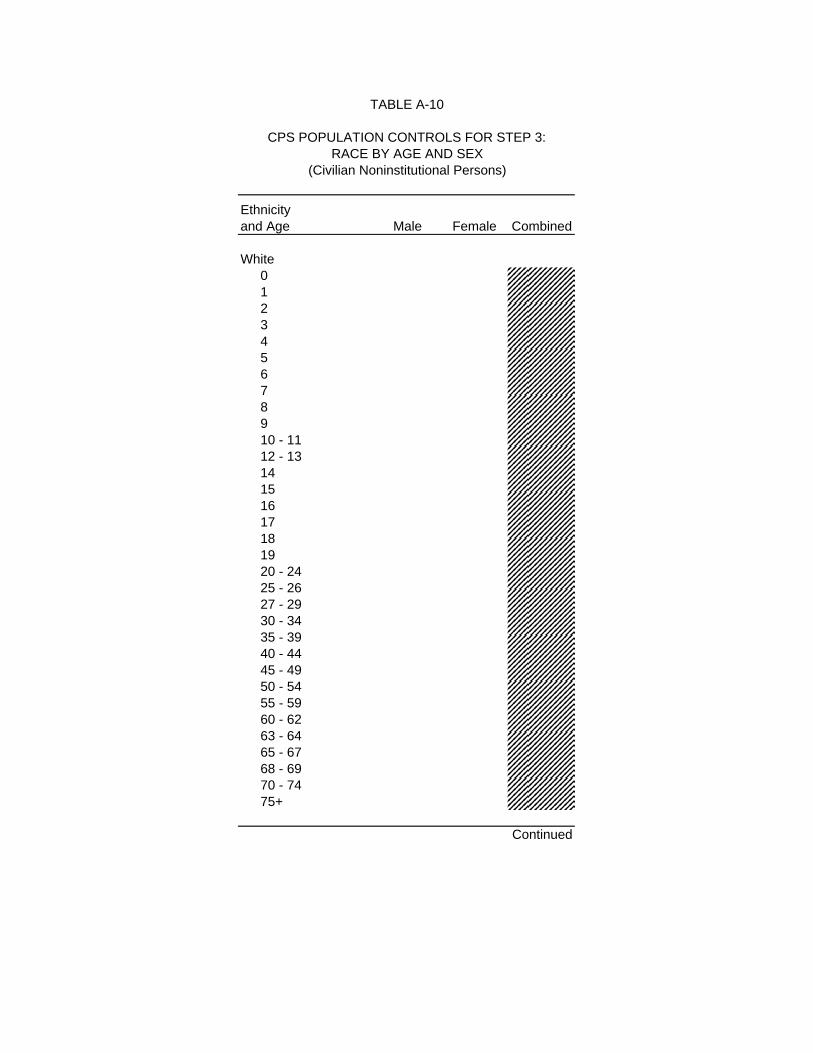
TABLE A-10

CPS POPULATION CONTROLS FOR STEP 3:RACE BY AGE AND SEX

(Civilian Noninstitutional Persons)

Ethnicityand Age Male Female Combined

White012345678910 - 1112 - 1314151617181920 - 2425 - 2627 - 2930 - 3435 - 3940 - 4445 - 4950 - 5455 - 5960 - 6263 - 6465 - 6768 - 6970 - 7475+

Continued

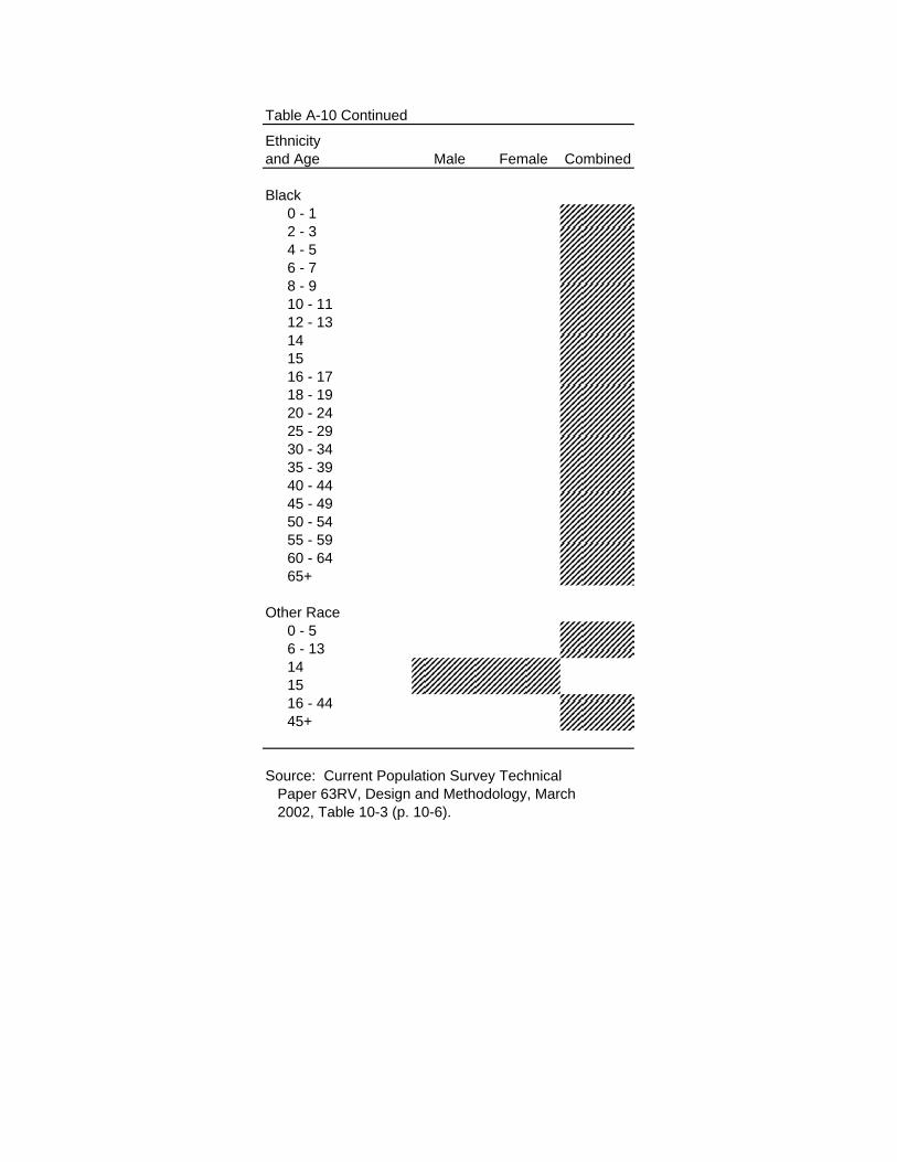
Table A-10 Continued

Ethnicityand Age Male Female Combined

Black0 - 12 - 34 - 56 - 78 - 910 - 1112 - 13141516 - 1718 - 1920 - 2425 - 2930 - 3435 - 3940 - 4445 - 4950 - 5455 - 5960 - 6465+

Other Race0 - 56 - 13141516 - 4445+

Source: Current Population Survey Technical Paper 63RV, Design and Methodology, March 2002, Table 10-3 (p. 10-6).

B-1

APPENDIX B

USE OF REPLICATE WEIGHTS TO CALCULATE STANDARD ERRORS FOR THE SIPP

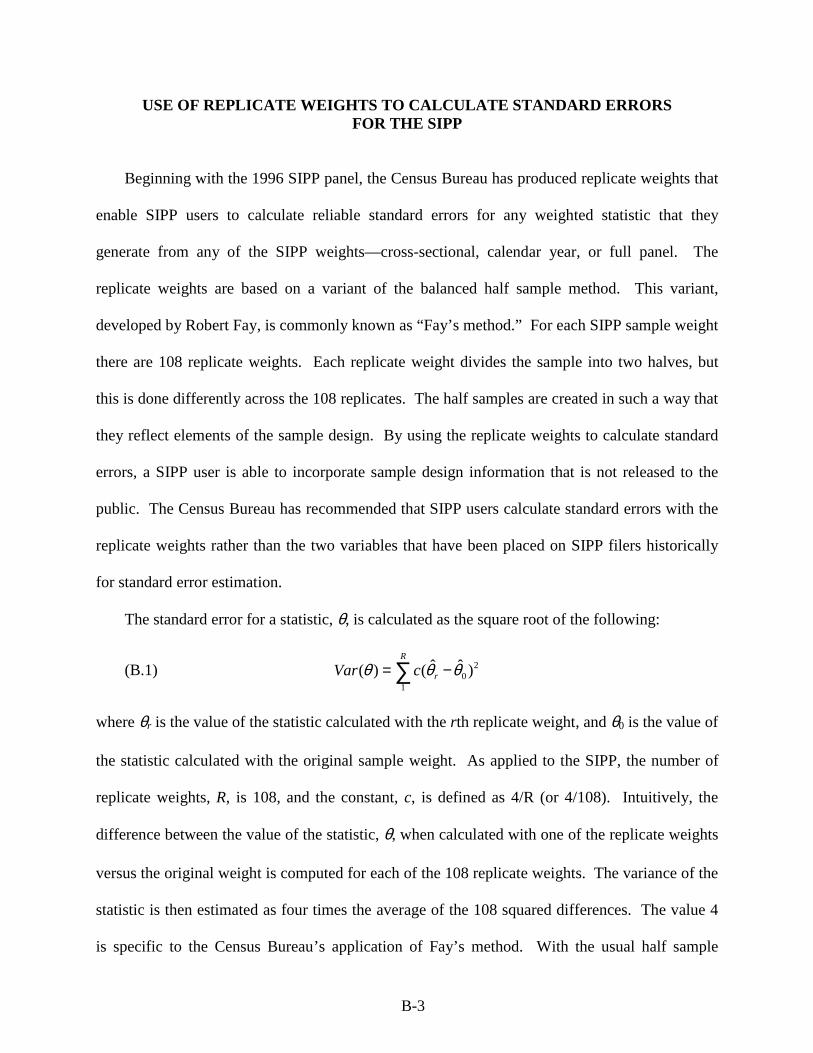
B-3

USE OF REPLICATE WEIGHTS TO CALCULATE STANDARD ERRORS FOR THE SIPP

Beginning with the 1996 SIPP panel, the Census Bureau has produced replicate weights that

enable SIPP users to calculate reliable standard errors for any weighted statistic that they

generate from any of the SIPP weights—cross-sectional, calendar year, or full panel. The

replicate weights are based on a variant of the balanced half sample method. This variant,

developed by Robert Fay, is commonly known as “Fay’s method.” For each SIPP sample weight

there are 108 replicate weights. Each replicate weight divides the sample into two halves, but

this is done differently across the 108 replicates. The half samples are created in such a way that

they reflect elements of the sample design. By using the replicate weights to calculate standard

errors, a SIPP user is able to incorporate sample design information that is not released to the

public. The Census Bureau has recommended that SIPP users calculate standard errors with the

replicate weights rather than the two variables that have been placed on SIPP filers historically

for standard error estimation.

The standard error for a statistic, θ, is calculated as the square root of the following:

(B.1) 20

1

ˆ ˆ( ) ( )R

rVar cθ θ θ= −∑

where θr is the value of the statistic calculated with the rth replicate weight, and θ0 is the value of

the statistic calculated with the original sample weight. As applied to the SIPP, the number of

replicate weights, R, is 108, and the constant, c, is defined as 4/R (or 4/108). Intuitively, the

difference between the value of the statistic, θ, when calculated with one of the replicate weights

versus the original weight is computed for each of the 108 replicate weights. The variance of the

statistic is then estimated as four times the average of the 108 squared differences. The value 4

is specific to the Census Bureau’s application of Fay’s method. With the usual half sample

B-4

method, only the records selected into a given half sample are used to estimate the statistic.

Implicitly, the weights on these records are multiplied by a factor of 1 while the weights on the

remaining half of the sample are multiplied by a factor of zero. Fay’s method replaces the 1 and

0 factors with 1.5 and 0.5. These factors are incorporated into the replicate weights.

Standard errors based on the SIPP replicate weights can be calculated for descriptive

statistics or regression coefficients with the software package SUDAAN, which can be accessed

through SAS. With each of the SUDAAN descriptive or regression procedures, the user can

specify that standard errors be calculated using the jackknife method and then identify the

variables that correspond to the original weight and the replicate weights. The user also provides

the value of c.

An example illustrates the use of SUDAAN to derive standard errors using SIPP replicate

weights. The following code, which was included in a SAS program, calls the SUDAAN

procedure “Descript” and specifies the calculation of descriptive statistics and standard errors for

two variables, “children” and “ehhnumpp.”

proc descript data= temp.test design = jackknife; title1 'standard errors using jackknife'; weight EHFNWGT1; jackwgts w1-w108 / adjjack=0.037037037037037037; var children ehhnumpp; print NSUM = "SAMPLE SIZE" WSUM = "POPULATION SIZE" TOTAL = "ROW TOTAL" SETOTAL = "STD ERR" SEMEAN = "STD ERR(Mean)" DEFFTOTAL = "DESIGN EFFECT"/ style = NCHS; run;

B-5

The statement in the first line, “design = jackknife” invokes the jackknife option. The original

weight, the replicate weights, and the value of the factor, c, are defined with the parameters

“weight,” “jackwgts,” and “adjjack.” The numeric term following this last parameter is the

value of 4/108. The statements under the print command provide labels and indicate a particular

output format (NCHS).

To apply this method to calculate the standard error of a difference of means for two

independent subpopulations (for example, the mean incomes of whites and nonwhites), one first

calculates the standard error for each mean, then derives the standard error of the difference as

the square root of the sum of the squares of the standard errors of the two means.

To calculate the standard error of a difference of means for a subpopulation and the

population from which that subpopulation was drawn (for example, a matched subsample and the

full sample, or the wave 1 sample members with full panel weights and all wave 1 sample

members), we replace the estimate of θr in equation B.1 with the difference between the

subpopulation and full population estimates of θ using the rth replicate weights, and we replace

the estimate of θ0 with the difference between the subpopulation and full population estimates

based on the original weights. If either of the original weights is calibrated, the replicate weights

must be calibrated as well (see Appendix A). Intuitively, the variance of the difference is

calculated as the variance of the 108 estimates of the difference, using the replicate weights,

around the original sample estimate of the difference. By calculating the test statistic directly,

the correlation between the subsample and full sample estimates is automatically taken into

account.

To calculate the standard error of a regression coefficient, one would use the SUDAAN

procedure “Regress” to estimate the coefficient and would specify the jackknife option with the

B-6

original weights, the replicate weights, and the value of the constant factor to obtain the desired

standard error.

C-1

APPENDIX C

COMPARISON OF MATCHED AND ENTIRE WAVE 1/WAVE 2 SAMPLES: 2001 SIPP PANEL

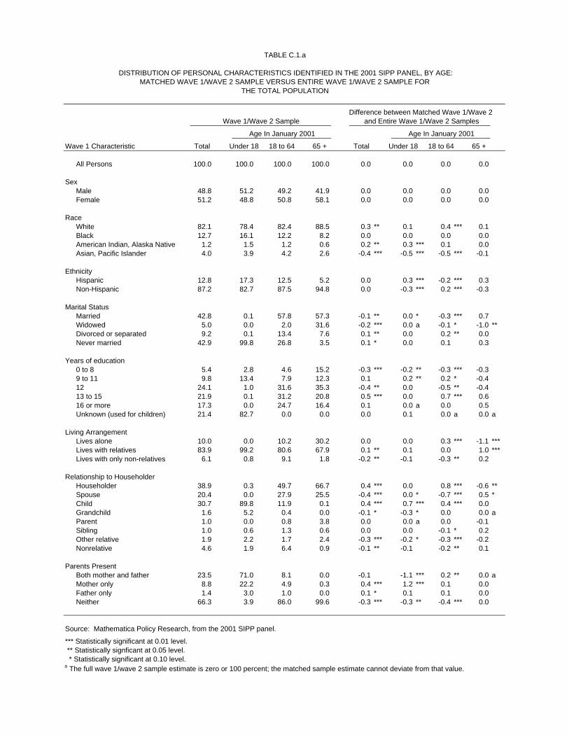
TABLE C.1.a

DISTRIBUTION OF PERSONAL CHARACTERISTICS IDENTIFIED IN THE 2001 SIPP PANEL, BY AGE:MATCHED WAVE 1/WAVE 2 SAMPLE VERSUS ENTIRE WAVE 1/WAVE 2 SAMPLE FOR

THE TOTAL POPULATION

Difference between Matched Wave 1/Wave 2Wave 1/Wave 2 Sample and Entire Wave 1/Wave 2 Samples

Age In January 2001 Age In January 2001

Wave 1 Characteristic Total Under 18 18 to 64 65 + Total Under 18 18 to 64 65 +

All Persons 100.0 100.0 100.0 100.0 0.0 0.0 0.0 0.0

SexMale 48.8 51.2 49.2 41.9 0.0 0.0 0.0 0.0 Female 51.2 48.8 50.8 58.1 0.0 0.0 0.0 0.0

RaceWhite 82.1 78.4 82.4 88.5 0.3 ** 0.1 0.4 *** 0.1 Black 12.7 16.1 12.2 8.2 0.0 0.0 0.0 0.0 American Indian, Alaska Native 1.2 1.5 1.2 0.6 0.2 ** 0.3 *** 0.1 0.0 Asian, Pacific Islander 4.0 3.9 4.2 2.6 -0.4 *** -0.5 *** -0.5 *** -0.1

EthnicityHispanic 12.8 17.3 12.5 5.2 0.0 0.3 *** -0.2 *** 0.3 Non-Hispanic 87.2 82.7 87.5 94.8 0.0 -0.3 *** 0.2 *** -0.3

Marital StatusMarried 42.8 0.1 57.8 57.3 -0.1 ** 0.0 * -0.3 *** 0.7 Widowed 5.0 0.0 2.0 31.6 -0.2 *** 0.0 a -0.1 * -1.0 **Divorced or separated 9.2 0.1 13.4 7.6 0.1 ** 0.0 0.2 ** 0.0 Never married 42.9 99.8 26.8 3.5 0.1 * 0.0 0.1 0.3

Years of education0 to 8 5.4 2.8 4.6 15.2 -0.3 *** -0.2 ** -0.3 *** -0.3 9 to 11 9.8 13.4 7.9 12.3 0.1 0.2 ** 0.2 * -0.4 12 24.1 1.0 31.6 35.3 -0.4 ** 0.0 -0.5 ** -0.4 13 to 15 21.9 0.1 31.2 20.8 0.5 *** 0.0 0.7 *** 0.6 16 or more 17.3 0.0 24.7 16.4 0.1 0.0 a 0.0 0.5 Unknown (used for children) 21.4 82.7 0.0 0.0 0.0 0.1 0.0 a 0.0 a

Living ArrangementLives alone 10.0 0.0 10.2 30.2 0.0 0.0 0.3 *** -1.1 ***Lives with relatives 83.9 99.2 80.6 67.9 0.1 ** 0.1 0.0 1.0 ***Lives with only non-relatives 6.1 0.8 9.1 1.8 -0.2 ** -0.1 -0.3 ** 0.2

Relationship to HouseholderHouseholder 38.9 0.3 49.7 66.7 0.4 *** 0.0 0.8 *** -0.6 **Spouse 20.4 0.0 27.9 25.5 -0.4 *** 0.0 * -0.7 *** 0.5 *Child 30.7 89.8 11.9 0.1 0.4 *** 0.7 *** 0.4 *** 0.0 Grandchild 1.6 5.2 0.4 0.0 -0.1 * -0.3 * 0.0 0.0 aParent 1.0 0.0 0.8 3.8 0.0 0.0 a 0.0 -0.1 Sibling 1.0 0.6 1.3 0.6 0.0 0.0 -0.1 * 0.2 Other relative 1.9 2.2 1.7 2.4 -0.3 *** -0.2 * -0.3 *** -0.2 Nonrelative 4.6 1.9 6.4 0.9 -0.1 ** -0.1 -0.2 ** 0.1

Parents PresentBoth mother and father 23.5 71.0 8.1 0.0 -0.1 -1.1 *** 0.2 ** 0.0 aMother only 8.8 22.2 4.9 0.3 0.4 *** 1.2 *** 0.1 0.0 Father only 1.4 3.0 1.0 0.0 0.1 * 0.1 0.1 0.0 Neither 66.3 3.9 86.0 99.6 -0.3 *** -0.3 ** -0.4 *** 0.0

Source: Mathematica Policy Research, from the 2001 SIPP panel.

*** Statistically significant at 0.01 level. ** Statistically signficant at 0.05 level. * Statistically significant at 0.10 level.a The full wave 1/wave 2 sample estimate is zero or 100 percent; the matched sample estimate cannot deviate from that value.

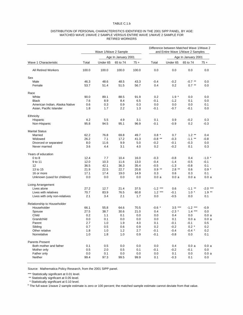
TABLE C.1.b

DISTRIBUTION OF PERSONAL CHARACTERISTICS IDENTIFIED IN THE 2001 SIPP PANEL, BY AGE:MATCHED WAVE 1/WAVE 2 SAMPLE VERSUS ENTIRE WAVE 1/WAVE 2 SAMPLE FOR

RETIRED WORKERS

Difference between Matched Wave 1/Wave 2Wave 1/Wave 2 Sample and Entire Wave 1/Wave 2 Samples

Age In January 2001 Age In January 2001

Wave 1 Characteristic Total Under 65 65 to 74 75 + Total Under 65 65 to 74 75 +

All Retired Workers 100.0 100.0 100.0 100.0 0.0 0.0 0.0 0.0

SexMale 46.3 48.6 48.5 43.3 -0.4 -0.2 -0.7 ** 0.0 Female 53.7 51.4 51.5 56.7 0.4 0.2 0.7 ** 0.0

RaceWhite 90.0 89.1 88.5 91.9 0.2 1.9 * 0.0 0.0 Black 7.6 8.9 8.4 6.5 -0.1 -1.2 0.1 0.0 American Indian, Alaska Native 0.6 0.3 0.9 0.3 0.0 0.0 0.0 0.1 Asian, Pacific Islander 1.8 1.7 2.2 1.3 -0.1 -0.7 -0.1 0.0

EthnicityHispanic 4.2 5.5 4.9 3.1 0.1 0.9 -0.2 0.3 Non-Hispanic 95.8 94.5 95.1 96.9 -0.1 -0.9 0.2 -0.3

Marital StatusMarried 62.2 76.8 69.8 49.7 0.8 * 0.7 1.2 ** 0.4 Widowed 26.2 7.1 17.2 41.3 -0.8 ** -0.3 -1.1 ** -0.8 Divorced or separated 8.0 11.6 9.9 5.0 -0.2 -0.1 -0.3 0.0 Never married 3.6 4.4 3.1 4.0 0.2 -0.2 0.1 0.3

Years of education0 to 8 12.4 7.7 10.4 16.0 -0.3 -0.8 0.4 -1.0 *9 to 11 12.0 10.3 11.6 13.0 -0.4 -1.4 -0.5 -0.1 12 36.5 42.1 36.3 35.4 -0.5 -1.3 -0.8 0.1 13 to 15 21.9 22.5 22.7 20.8 0.9 ** 2.8 ** 0.6 0.9 *16 or more 17.1 17.4 19.0 14.9 0.3 0.6 0.3 0.1 Unknown (used for children) 0.0 0.0 0.0 0.0 0.0 a 0.0 a 0.0 a 0.0 a

Living ArrangementLives alone 27.2 12.7 21.4 37.5 -1.2 *** 0.6 -1.1 ** -2.0 ***Lives with relatives 70.7 83.9 76.5 60.8 1.2 *** -0.1 1.0 * 1.9 **Lives with only non-relatives 2.1 3.4 2.1 1.7 0.0 -0.5 0.0 0.1

Relationship to HouseholderHouseholder 66.1 55.8 64.6 70.5 -0.6 * 3.5 *** -1.2 *** -0.9 Spouse 27.5 38.7 30.6 21.0 0.4 -2.3 * 1.4 *** 0.0 Child 0.2 1.1 0.1 0.0 0.0 0.4 0.0 0.0 aGrandchild 0.0 0.1 0.0 0.0 0.0 0.1 0.0 a 0.0 aParent 2.7 1.0 1.9 4.0 0.1 -0.1 -0.1 0.5 Sibling 0.7 0.5 0.6 0.9 0.2 -0.2 0.2 * 0.2 Other relative 1.8 1.0 1.2 2.7 -0.1 -0.4 -0.4 * 0.2 Nonrelative 1.0 1.8 1.0 0.9 -0.1 -0.8 0.0 0.1

Parents PresentBoth mother and father 0.1 0.5 0.0 0.0 0.0 0.4 0.0 a 0.0 aMother only 0.5 2.0 0.5 0.1 -0.1 -0.2 -0.1 0.0 Father only 0.0 0.1 0.0 0.0 0.0 0.1 0.0 0.0 aNeither 99.4 97.3 99.5 99.9 0.1 -0.3 0.1 0.0

Source: Mathematica Policy Research, from the 2001 SIPP panel.

*** Statistically significant at 0.01 level. ** Statistically signficant at 0.05 level. * Statistically significant at 0.10 level.a The full wave 1/wave 2 sample estimate is zero or 100 percent; the matched sample estimate cannot deviate from that value.

TABLE C.1.c

DISTRIBUTION OF PERSONAL CHARACTERISTICS IDENTIFIED IN THE 2001 SIPP PANEL, BY AGE:MATCHED WAVE 1/WAVE 2 SAMPLE VERSUS ENTIRE WAVE 1/WAVE 2 SAMPLE FOR

DISABLED WORKERS

Difference between Matched Wave 1/Wave 2Wave 1/Wave 2 Sample and Entire Wave 1/Wave 2 Samples

Age In January 2001 Age In January 2001

Wave 1 Characteristic Total Under 50 50 to 64 65 + Total Under 50 50 to 64 65 +

All Disabled Workers 100.0 100.0 100.0 100.0 0.0 0.0 0.0 0.0

SexMale 51.8 54.3 52.9 45.9 -0.7 -0.9 -1.2 0.1 Female 48.2 45.7 47.1 54.1 0.7 0.9 1.2 -0.1

RaceWhite 78.0 76.7 78.4 78.9 -1.6 ** -0.8 -1.5 -2.7 Black 19.1 20.2 19.0 17.5 1.1 1.0 1.2 1.1 American Indian, Alaska Native 1.1 0.9 1.5 0.5 0.3 ** 0.4 ** 0.3 0.3 Asian, Pacific Islander 1.9 2.2 1.1 3.0 0.1 -0.5 -0.1 1.3 ***

EthnicityHispanic 9.1 9.0 8.3 10.8 1.2 ** 0.7 0.9 2.2 *Non-Hispanic 90.9 91.0 91.7 89.2 -1.2 ** -0.7 -0.9 -2.2 *

Marital StatusMarried 45.3 31.2 54.9 48.7 0.3 0.2 1.9 -0.6 Widowed 10.6 1.7 8.5 27.6 -0.5 -1.1 ** 0.9 -1.5 Divorced or separated 22.6 19.0 27.5 19.0 -0.2 0.1 -0.8 1.1 Never married 21.5 48.1 9.2 4.7 0.4 0.9 -2.0 * 1.1

Years of education0 to 8 17.8 11.0 16.1 30.9 0.4 1.5 -1.9 3.0 9 to 11 15.7 13.5 16.1 18.0 -0.7 -1.0 -0.4 -0.6 12 37.4 41.2 38.0 30.6 -0.2 0.4 -0.2 -1.3 13 to 15 23.6 28.8 23.3 16.4 -0.1 -2.3 2.4 * -1.7 16 or more 5.6 5.5 6.5 4.0 0.6 1.3 ** 0.1 0.6 Unknown (used for children) 0.0 0.0 0.0 0.0 0.0 a 0.0 a 0.0 a 0.0 a

Living ArrangementLives alone 23.5 17.7 22.7 33.5 0.0 0.2 -0.2 0.5 Lives with relatives 69.6 71.2 72.1 62.6 0.8 1.1 2.0 -1.5 Lives with only non-relatives 6.9 11.0 5.2 3.9 -0.9 -1.3 -1.7 ** 0.9

Relationship to HouseholderHouseholder 60.8 50.2 64.5 69.6 0.4 -2.6 2.6 2.4 Spouse 18.7 12.5 23.8 18.1 0.1 1.2 1.1 -2.6 Child 10.0 24.5 3.7 0.0 0.5 2.1 -1.5 * 0.0 aGrandchild 0.3 0.7 0.0 0.0 0.1 0.1 0.0 a 0.0 aParent 2.1 0.2 1.9 5.1 0.0 0.1 0.4 -0.8 Sibling 1.7 2.0 1.8 1.2 0.1 0.5 -0.7 0.7 Other relative 2.4 1.9 1.9 3.8 -0.2 0.1 -0.4 -0.4 Nonrelative 4.2 7.9 2.4 2.2 -0.9 * -1.5 -1.6 ** 0.7

Parents PresentBoth mother and father 4.2 11.5 0.7 0.0 0.7 1.7 -0.1 0.0 aMother only 6.9 14.6 4.5 0.0 0.0 0.1 -0.4 0.0 aFather only 0.6 1.4 0.3 0.0 0.2 0.5 0.1 0.0 aNeither 88.2 72.5 94.5 100.0 -1.0 -2.3 0.5 0.0 a

Source: Mathematica Policy Research, from the 2001 SIPP panel.

*** Statistically significant at 0.01 level. ** Statistically signficant at 0.05 level. * Statistically significant at 0.10 level.a The full wave 1/wave 2 sample estimate is zero or 100 percent; the matched sample estimate cannot deviate from that value.

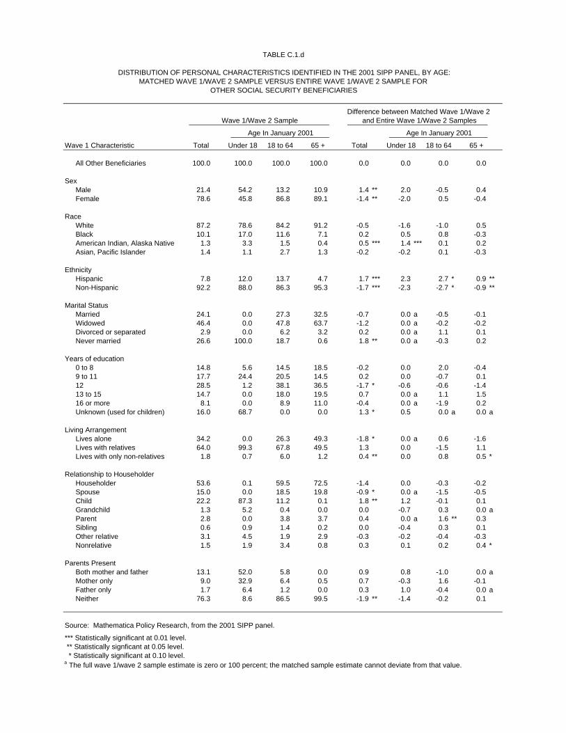
TABLE C.1.d

DISTRIBUTION OF PERSONAL CHARACTERISTICS IDENTIFIED IN THE 2001 SIPP PANEL, BY AGE:MATCHED WAVE 1/WAVE 2 SAMPLE VERSUS ENTIRE WAVE 1/WAVE 2 SAMPLE FOR

OTHER SOCIAL SECURITY BENEFICIARIES

Difference between Matched Wave 1/Wave 2Wave 1/Wave 2 Sample and Entire Wave 1/Wave 2 Samples

Age In January 2001 Age In January 2001

Wave 1 Characteristic Total Under 18 18 to 64 65 + Total Under 18 18 to 64 65 +

All Other Beneficiaries 100.0 100.0 100.0 100.0 0.0 0.0 0.0 0.0

SexMale 21.4 54.2 13.2 10.9 1.4 ** 2.0 -0.5 0.4 Female 78.6 45.8 86.8 89.1 -1.4 ** -2.0 0.5 -0.4

RaceWhite 87.2 78.6 84.2 91.2 -0.5 -1.6 -1.0 0.5 Black 10.1 17.0 11.6 7.1 0.2 0.5 0.8 -0.3 American Indian, Alaska Native 1.3 3.3 1.5 0.4 0.5 *** 1.4 *** 0.1 0.2 Asian, Pacific Islander 1.4 1.1 2.7 1.3 -0.2 -0.2 0.1 -0.3

EthnicityHispanic 7.8 12.0 13.7 4.7 1.7 *** 2.3 2.7 * 0.9 **Non-Hispanic 92.2 88.0 86.3 95.3 -1.7 *** -2.3 -2.7 * -0.9 **

Marital StatusMarried 24.1 0.0 27.3 32.5 -0.7 0.0 a -0.5 -0.1 Widowed 46.4 0.0 47.8 63.7 -1.2 0.0 a -0.2 -0.2 Divorced or separated 2.9 0.0 6.2 3.2 0.2 0.0 a 1.1 0.1 Never married 26.6 100.0 18.7 0.6 1.8 ** 0.0 a -0.3 0.2

Years of education0 to 8 14.8 5.6 14.5 18.5 -0.2 0.0 2.0 -0.4 9 to 11 17.7 24.4 20.5 14.5 0.2 0.0 -0.7 0.1 12 28.5 1.2 38.1 36.5 -1.7 * -0.6 -0.6 -1.4 13 to 15 14.7 0.0 18.0 19.5 0.7 0.0 a 1.1 1.5 16 or more 8.1 0.0 8.9 11.0 -0.4 0.0 a -1.9 0.2 Unknown (used for children) 16.0 68.7 0.0 0.0 1.3 * 0.5 0.0 a 0.0 a

Living ArrangementLives alone 34.2 0.0 26.3 49.3 -1.8 * 0.0 a 0.6 -1.6 Lives with relatives 64.0 99.3 67.8 49.5 1.3 0.0 -1.5 1.1 Lives with only non-relatives 1.8 0.7 6.0 1.2 0.4 ** 0.0 0.8 0.5 *

Relationship to HouseholderHouseholder 53.6 0.1 59.5 72.5 -1.4 0.0 -0.3 -0.2 Spouse 15.0 0.0 18.5 19.8 -0.9 * 0.0 a -1.5 -0.5 Child 22.2 87.3 11.2 0.1 1.8 ** 1.2 -0.1 0.1 Grandchild 1.3 5.2 0.4 0.0 0.0 -0.7 0.3 0.0 aParent 2.8 0.0 3.8 3.7 0.4 0.0 a 1.6 ** 0.3 Sibling 0.6 0.9 1.4 0.2 0.0 -0.4 0.3 0.1 Other relative 3.1 4.5 1.9 2.9 -0.3 -0.2 -0.4 -0.3 Nonrelative 1.5 1.9 3.4 0.8 0.3 0.1 0.2 0.4 *

Parents PresentBoth mother and father 13.1 52.0 5.8 0.0 0.9 0.8 -1.0 0.0 aMother only 9.0 32.9 6.4 0.5 0.7 -0.3 1.6 -0.1 Father only 1.7 6.4 1.2 0.0 0.3 1.0 -0.4 0.0 aNeither 76.3 8.6 86.5 99.5 -1.9 ** -1.4 -0.2 0.1

Source: Mathematica Policy Research, from the 2001 SIPP panel.

*** Statistically significant at 0.01 level. ** Statistically signficant at 0.05 level. * Statistically significant at 0.10 level.a The full wave 1/wave 2 sample estimate is zero or 100 percent; the matched sample estimate cannot deviate from that value.

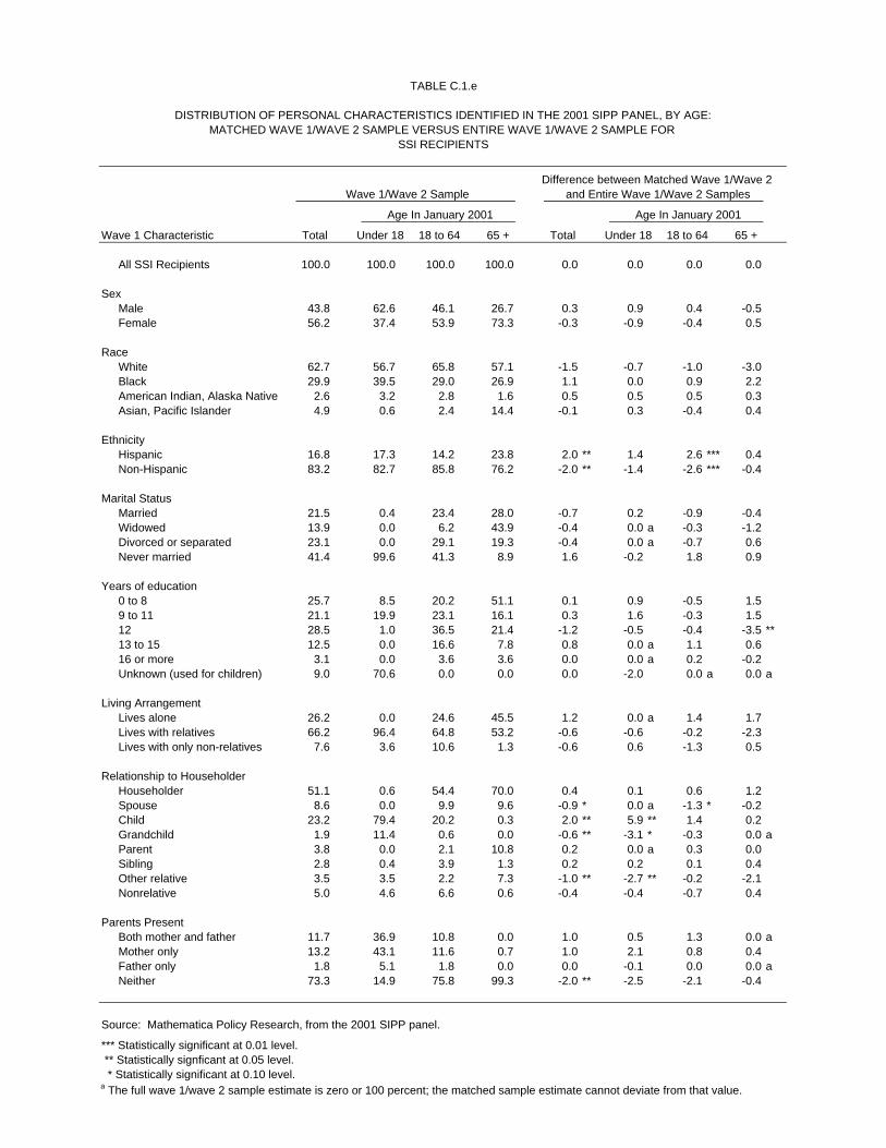
TABLE C.1.e

DISTRIBUTION OF PERSONAL CHARACTERISTICS IDENTIFIED IN THE 2001 SIPP PANEL, BY AGE:MATCHED WAVE 1/WAVE 2 SAMPLE VERSUS ENTIRE WAVE 1/WAVE 2 SAMPLE FOR

SSI RECIPIENTS

Difference between Matched Wave 1/Wave 2Wave 1/Wave 2 Sample and Entire Wave 1/Wave 2 Samples

Age In January 2001 Age In January 2001

Wave 1 Characteristic Total Under 18 18 to 64 65 + Total Under 18 18 to 64 65 +

All SSI Recipients 100.0 100.0 100.0 100.0 0.0 0.0 0.0 0.0

SexMale 43.8 62.6 46.1 26.7 0.3 0.9 0.4 -0.5 Female 56.2 37.4 53.9 73.3 -0.3 -0.9 -0.4 0.5

RaceWhite 62.7 56.7 65.8 57.1 -1.5 -0.7 -1.0 -3.0 Black 29.9 39.5 29.0 26.9 1.1 0.0 0.9 2.2 American Indian, Alaska Native 2.6 3.2 2.8 1.6 0.5 0.5 0.5 0.3 Asian, Pacific Islander 4.9 0.6 2.4 14.4 -0.1 0.3 -0.4 0.4

EthnicityHispanic 16.8 17.3 14.2 23.8 2.0 ** 1.4 2.6 *** 0.4 Non-Hispanic 83.2 82.7 85.8 76.2 -2.0 ** -1.4 -2.6 *** -0.4

Marital StatusMarried 21.5 0.4 23.4 28.0 -0.7 0.2 -0.9 -0.4 Widowed 13.9 0.0 6.2 43.9 -0.4 0.0 a -0.3 -1.2 Divorced or separated 23.1 0.0 29.1 19.3 -0.4 0.0 a -0.7 0.6 Never married 41.4 99.6 41.3 8.9 1.6 -0.2 1.8 0.9

Years of education0 to 8 25.7 8.5 20.2 51.1 0.1 0.9 -0.5 1.5 9 to 11 21.1 19.9 23.1 16.1 0.3 1.6 -0.3 1.5 12 28.5 1.0 36.5 21.4 -1.2 -0.5 -0.4 -3.5 **13 to 15 12.5 0.0 16.6 7.8 0.8 0.0 a 1.1 0.6 16 or more 3.1 0.0 3.6 3.6 0.0 0.0 a 0.2 -0.2 Unknown (used for children) 9.0 70.6 0.0 0.0 0.0 -2.0 0.0 a 0.0 a

Living ArrangementLives alone 26.2 0.0 24.6 45.5 1.2 0.0 a 1.4 1.7 Lives with relatives 66.2 96.4 64.8 53.2 -0.6 -0.6 -0.2 -2.3 Lives with only non-relatives 7.6 3.6 10.6 1.3 -0.6 0.6 -1.3 0.5

Relationship to HouseholderHouseholder 51.1 0.6 54.4 70.0 0.4 0.1 0.6 1.2 Spouse 8.6 0.0 9.9 9.6 -0.9 * 0.0 a -1.3 * -0.2 Child 23.2 79.4 20.2 0.3 2.0 ** 5.9 ** 1.4 0.2 Grandchild 1.9 11.4 0.6 0.0 -0.6 ** -3.1 * -0.3 0.0 aParent 3.8 0.0 2.1 10.8 0.2 0.0 a 0.3 0.0 Sibling 2.8 0.4 3.9 1.3 0.2 0.2 0.1 0.4 Other relative 3.5 3.5 2.2 7.3 -1.0 ** -2.7 ** -0.2 -2.1 Nonrelative 5.0 4.6 6.6 0.6 -0.4 -0.4 -0.7 0.4

Parents PresentBoth mother and father 11.7 36.9 10.8 0.0 1.0 0.5 1.3 0.0 aMother only 13.2 43.1 11.6 0.7 1.0 2.1 0.8 0.4 Father only 1.8 5.1 1.8 0.0 0.0 -0.1 0.0 0.0 aNeither 73.3 14.9 75.8 99.3 -2.0 ** -2.5 -2.1 -0.4

Source: Mathematica Policy Research, from the 2001 SIPP panel.

*** Statistically significant at 0.01 level. ** Statistically signficant at 0.05 level. * Statistically significant at 0.10 level.a The full wave 1/wave 2 sample estimate is zero or 100 percent; the matched sample estimate cannot deviate from that value.

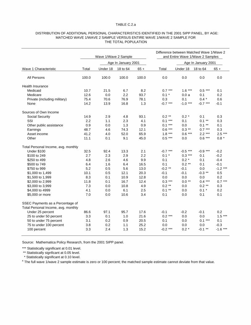
TABLE C.2.a

DISTRIBUTION OF ADDITIONAL PERSONAL CHARACTERISTICS IDENTIFIED IN THE 2001 SIPP PANEL, BY AGE:MATCHED WAVE 1/WAVE 2 SAMPLE VERSUS ENTIRE WAVE 1/WAVE 2 SAMPLE FOR

THE TOTAL POPULATION

Difference between Matched Wave 1/Wave 2Wave 1/Wave 2 Sample and Entire Wave 1/Wave 2 Samples

Age In January 2001 Age In January 2001

Wave 1 Characteristic Total Under 18 18 to 64 65 + Total Under 18 18 to 64 65 +

All Persons 100.0 100.0 100.0 100.0 0.0 0.0 0.0 0.0

Health InsuranceMedicaid 10.7 21.5 6.7 8.2 0.7 *** 1.6 *** 0.5 *** 0.1 Medicare 12.6 0.0 2.2 93.7 0.1 * 0.0 a 0.1 0.2 Private (including military) 75.4 70.6 76.9 78.1 0.3 0.1 0.4 * 0.6 None 14.2 13.9 16.8 1.3 -0.7 *** -1.0 *** -0.7 *** -0.1

Sources of Own IncomeSocial Security 14.9 2.9 4.8 93.1 0.2 ** 0.2 * 0.1 0.3 SSI 2.2 1.1 2.3 4.1 0.1 *** 0.1 0.1 ** 0.3 Other public assistance 0.9 0.0 1.3 0.9 0.1 *** 0.0 0.1 ** 0.1 Earnings 48.7 4.6 74.3 12.1 0.6 *** 0.3 ** 0.7 *** 0.3 Asset income 41.2 4.0 52.0 65.9 1.8 *** 0.6 *** 2.2 *** 2.5 ***Other 11.1 0.1 9.1 45.0 0.5 *** 0.0 0.6 *** 0.8 *

Total Personal Income, avg. monthlyUnder $100 32.5 92.4 13.3 2.1 -0.7 *** -0.5 *** -0.9 *** -0.2 $100 to 249 2.7 2.3 2.9 2.2 0.1 * 0.3 *** 0.1 -0.2 $250 to 499 4.8 2.6 4.6 9.9 0.1 0.2 * 0.1 -0.4 $500 to 749 6.4 1.6 6.4 16.5 0.1 0.2 ** 0.1 -0.1 $750 to 999 5.2 0.5 5.6 13.0 -0.2 ** -0.1 0.0 -1.2 ***$1,000 to 1,499 10.1 0.5 12.1 20.3 -0.1 -0.1 -0.3 ** 0.5 $1,500 to 1,999 8.3 0.1 10.9 12.8 0.0 0.0 0.0 0.2 $2,000 to 2,999 11.8 0.1 16.7 12.4 0.3 *** 0.0 ** 0.4 *** 0.7 ***$3,000 to 3,999 7.3 0.0 10.8 4.9 0.2 ** 0.0 0.2 ** 0.3 $4,000 to 4999 4.1 0.0 6.1 2.5 0.1 ** 0.0 0.1 * 0.2 $5,000 or more 7.0 0.0 10.6 3.4 0.1 0.0 0.1 0.1

SSEC Payments as a Percentage ofTotal Personal Income, avg. monthly

Under 25 percent 86.6 97.1 95.7 17.6 -0.1 -0.2 -0.1 0.2 25 to under 50 percent 3.3 0.1 1.0 21.6 0.2 *** 0.0 0.0 1.5 ***50 to under 75 percent 3.1 0.2 0.9 20.5 0.1 0.0 0.1 *** 0.1 75 to under 100 percent 3.8 0.2 1.1 25.2 0.0 0.0 0.0 -0.3 100 percent 3.3 2.4 1.3 15.2 -0.2 *** 0.2 * -0.1 ** -1.6 ***

Source: Mathematica Policy Research, from the 2001 SIPP panel.

*** Statistically significant at 0.01 level. ** Statistically signficant at 0.05 level. * Statistically significant at 0.10 level.a The full wave 1/wave 2 sample estimate is zero or 100 percent; the matched sample estimate cannot deviate from that value.

TABLE C.2.b

DISTRIBUTION OF ADDITIONAL PERSONAL CHARACTERISTICS IDENTIFIED IN THE 2001 SIPP PANEL, BY AGE:MATCHED WAVE 1/WAVE 2 SAMPLE VERSUS ENTIRE WAVE 1/WAVE 2 SAMPLE FOR

RETIRED WORKERS

Difference between Matched Wave 1/Wave 2Wave 1/Wave 2 Sample and Entire Wave 1/Wave 2 Samples

Age In January 2001 Age In January 2001

Wave 1 Characteristic Total Under 65 65 to 74 75 + Total Under 65 65 to 74 75 +

All Retired Workers 100.0 100.0 100.0 100.0 0.0 0.0 0.0 0.0

Health InsuranceMedicaid 5.8 5.8 5.7 6.0 0.1 0.0 0.4 -0.3 Medicare 91.5 19.0 99.9 100.0 0.1 -1.7 0.0 0.0 aPrivate (including military) 80.7 79.6 81.2 80.4 0.3 -0.7 0.6 0.2 None 1.1 10.4 0.0 0.0 0.0 0.4 0.0 0.0 a

Sources of Own IncomeSocial Security 100.0 100.0 100.0 100.0 0.0 a 0.0 a 0.0 a 0.0 aSSI 2.2 2.7 2.2 2.1 0.2 -0.2 0.4 ** 0.0 Other public assistance 0.6 0.2 0.6 0.8 0.1 0.1 0.0 0.2 Earnings 12.6 22.5 17.1 5.0 0.3 2.7 ** 0.0 0.3 Asset income 68.3 62.7 68.0 70.1 2.4 *** 4.8 *** 2.5 *** 1.6 **Other 47.8 42.5 46.9 50.1 1.1 ** 1.8 0.7 1.2

Total Personal Income, avg. monthlyUnder $100 0.5 0.7 0.5 0.4 0.0 -0.2 0.0 -0.1 $100 to 249 1.9 2.2 2.0 1.6 -0.2 -0.3 -0.1 -0.3 $250 to 499 9.6 10.5 10.1 8.7 -0.1 0.8 -0.3 -0.1 $500 to 749 15.0 12.9 13.7 17.0 -0.2 -0.6 -0.1 -0.2 $750 to 999 13.2 12.7 12.0 14.6 -1.0 *** -0.1 -0.6 -1.7 ***$1,000 to 1,499 20.9 17.0 20.0 23.0 0.5 -0.1 0.1 1.0 $1,500 to 1,999 13.8 11.9 13.5 14.5 0.3 -0.2 0.5 0.2 $2,000 to 2,999 13.7 15.3 14.9 11.8 0.5 * -0.3 0.6 0.7 *$3,000 to 3,999 5.6 9.6 6.0 4.3 0.2 1.3 0.0 0.2 $4,000 to 4999 2.8 4.0 3.3 1.8 0.1 -0.5 0.2 0.2 $5,000 or more 3.2 3.3 3.9 2.3 0.0 0.3 -0.2 0.2

SSEC Payments as a Percentage ofTotal Personal Income, avg. monthly

Under 25 percent 11.8 16.3 13.7 8.5 0.2 -0.8 0.0 0.8 **25 to under 50 percent 24.7 29.1 25.4 22.8 1.6 *** 1.1 1.6 *** 1.6 **50 to under 75 percent 22.3 18.7 22.3 23.1 0.3 2.5 ** 0.5 -0.6 75 to under 100 percent 26.1 18.9 24.2 30.1 -0.3 0.1 -0.3 -0.6 100 percent 15.1 17.1 14.4 15.5 -1.7 *** -2.9 ** -1.8 *** -1.3 **

Source: Mathematica Policy Research, from the 2001 SIPP panel.

*** Statistically significant at 0.01 level. ** Statistically signficant at 0.05 level. * Statistically significant at 0.10 level.a The full wave 1/wave 2 sample estimate is zero or 100 percent; the matched sample estimate cannot deviate from that value.

TABLE C.2.c

DISTRIBUTION OF ADDITIONAL PERSONAL CHARACTERISTICS IDENTIFIED IN THE 2001 SIPP PANEL, BY AGE:MATCHED WAVE 1/WAVE 2 SAMPLE VERSUS ENTIRE WAVE 1/WAVE 2 SAMPLE FOR

DISABLED WORKERS

Difference between Matched Wave 1/Wave 2Wave 1/Wave 2 Sample and Entire Wave 1/Wave 2 Samples

Age In January 2001 Age In January 2001

Wave 1 Characteristic Total Under 50 50 to 64 65 + Total Under 50 50 to 64 65 +

All Disabled Workers 100.0 100.0 100.0 100.0 0.0 0.0 0.0 0.0

Health InsuranceMedicaid 35.9 50.6 26.9 30.7 2.4 ** 1.6 1.8 3.2 Medicare 78.5 71.6 72.3 100.0 1.6 * 2.1 2.1 0.0 aPrivate (including military) 43.1 31.9 45.7 54.8 -0.4 2.0 0.1 -4.0 *None 2.8 3.4 3.8 0.0 -0.1 0.5 -0.6 0.0 a

Sources of Own IncomeSocial Security 100.0 100.0 100.0 100.0 0.0 a 0.0 a 0.0 a 0.0 aSSI 18.5 26.9 14.3 13.8 0.8 0.5 0.4 1.3 Other public assistance 3.8 5.7 3.0 2.4 0.6 * 0.1 0.4 1.5 ***Earnings 7.8 14.6 4.3 4.2 1.2 ** 2.4 * 0.4 0.1 Asset income 30.8 23.4 32.7 38.3 1.9 * -0.7 4.1 ** 2.8 Other 25.5 16.6 29.0 32.0 0.9 0.4 1.5 1.4

Total Personal Income, avg. monthlyUnder $100 0.6 0.6 0.6 0.7 -0.2 -0.4 *** -0.2 0.3 $100 to 249 1.9 1.9 2.0 1.6 0.4 0.8 *** 0.3 0.0 $250 to 499 9.3 8.4 8.1 12.7 -1.2 * -1.2 -1.4 -0.9 $500 to 749 32.0 40.2 26.5 30.0 -0.1 -0.6 -0.6 0.5 $750 to 999 19.2 18.0 21.2 17.3 0.7 1.6 0.9 -0.6 $1,000 to 1,499 20.5 18.0 23.0 19.6 -0.7 -0.9 0.5 -2.1 $1,500 to 1,999 6.4 5.9 6.0 8.0 0.4 0.4 0.0 0.9 $2,000 to 2,999 6.5 4.8 7.1 7.9 1.1 ** 0.5 1.3 1.7 *$3,000 to 3,999 2.3 1.2 3.7 1.4 0.2 0.4 -0.1 0.7 *$4,000 to 4999 0.5 0.1 0.7 0.5 -0.2 -0.1 -0.3 -0.2 $5,000 or more 0.8 0.8 1.0 0.3 -0.4 ** -0.5 -0.4 -0.3

SSEC Payments as a Percentage ofTotal Personal Income, avg. monthly

Under 25 percent 5.0 7.8 3.8 3.3 0.1 0.3 -0.8 0.8 25 to under 50 percent 13.6 14.3 12.9 14.1 0.9 0.9 -0.1 2.5 *50 to under 75 percent 19.6 19.3 17.3 24.2 2.2 ** 1.5 3.4 ** 0.8 75 to under 100 percent 25.9 23.5 28.0 25.4 0.5 0.3 1.8 -1.1 100 percent 35.9 35.1 38.0 33.1 -3.6 *** -3.0 * -4.3 ** -2.9

Source: Mathematica Policy Research, from the 2001 SIPP panel.

*** Statistically significant at 0.01 level. ** Statistically signficant at 0.05 level. * Statistically significant at 0.10 level.a The full wave 1/wave 2 sample estimate is zero or 100 percent; the matched sample estimate cannot deviate from that value.

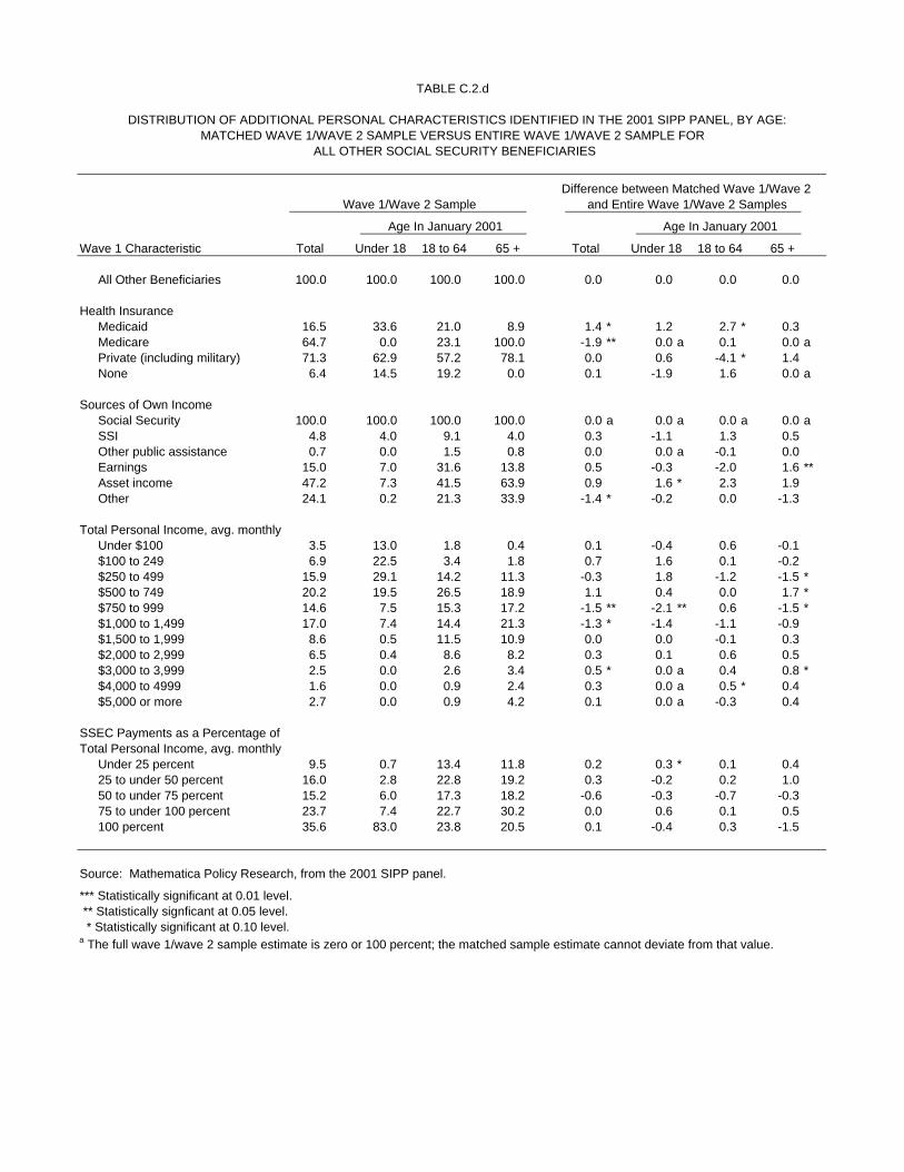
TABLE C.2.d

DISTRIBUTION OF ADDITIONAL PERSONAL CHARACTERISTICS IDENTIFIED IN THE 2001 SIPP PANEL, BY AGE:MATCHED WAVE 1/WAVE 2 SAMPLE VERSUS ENTIRE WAVE 1/WAVE 2 SAMPLE FOR

ALL OTHER SOCIAL SECURITY BENEFICIARIES

Difference between Matched Wave 1/Wave 2Wave 1/Wave 2 Sample and Entire Wave 1/Wave 2 Samples

Age In January 2001 Age In January 2001

Wave 1 Characteristic Total Under 18 18 to 64 65 + Total Under 18 18 to 64 65 +

All Other Beneficiaries 100.0 100.0 100.0 100.0 0.0 0.0 0.0 0.0

Health InsuranceMedicaid 16.5 33.6 21.0 8.9 1.4 * 1.2 2.7 * 0.3 Medicare 64.7 0.0 23.1 100.0 -1.9 ** 0.0 a 0.1 0.0 aPrivate (including military) 71.3 62.9 57.2 78.1 0.0 0.6 -4.1 * 1.4 None 6.4 14.5 19.2 0.0 0.1 -1.9 1.6 0.0 a

Sources of Own IncomeSocial Security 100.0 100.0 100.0 100.0 0.0 a 0.0 a 0.0 a 0.0 aSSI 4.8 4.0 9.1 4.0 0.3 -1.1 1.3 0.5 Other public assistance 0.7 0.0 1.5 0.8 0.0 0.0 a -0.1 0.0 Earnings 15.0 7.0 31.6 13.8 0.5 -0.3 -2.0 1.6 **Asset income 47.2 7.3 41.5 63.9 0.9 1.6 * 2.3 1.9 Other 24.1 0.2 21.3 33.9 -1.4 * -0.2 0.0 -1.3

Total Personal Income, avg. monthlyUnder $100 3.5 13.0 1.8 0.4 0.1 -0.4 0.6 -0.1 $100 to 249 6.9 22.5 3.4 1.8 0.7 1.6 0.1 -0.2 $250 to 499 15.9 29.1 14.2 11.3 -0.3 1.8 -1.2 -1.5 *$500 to 749 20.2 19.5 26.5 18.9 1.1 0.4 0.0 1.7 *$750 to 999 14.6 7.5 15.3 17.2 -1.5 ** -2.1 ** 0.6 -1.5 *$1,000 to 1,499 17.0 7.4 14.4 21.3 -1.3 * -1.4 -1.1 -0.9 $1,500 to 1,999 8.6 0.5 11.5 10.9 0.0 0.0 -0.1 0.3 $2,000 to 2,999 6.5 0.4 8.6 8.2 0.3 0.1 0.6 0.5 $3,000 to 3,999 2.5 0.0 2.6 3.4 0.5 * 0.0 a 0.4 0.8 *$4,000 to 4999 1.6 0.0 0.9 2.4 0.3 0.0 a 0.5 * 0.4 $5,000 or more 2.7 0.0 0.9 4.2 0.1 0.0 a -0.3 0.4

SSEC Payments as a Percentage ofTotal Personal Income, avg. monthly

Under 25 percent 9.5 0.7 13.4 11.8 0.2 0.3 * 0.1 0.4 25 to under 50 percent 16.0 2.8 22.8 19.2 0.3 -0.2 0.2 1.0 50 to under 75 percent 15.2 6.0 17.3 18.2 -0.6 -0.3 -0.7 -0.3 75 to under 100 percent 23.7 7.4 22.7 30.2 0.0 0.6 0.1 0.5 100 percent 35.6 83.0 23.8 20.5 0.1 -0.4 0.3 -1.5

Source: Mathematica Policy Research, from the 2001 SIPP panel.

*** Statistically significant at 0.01 level. ** Statistically signficant at 0.05 level. * Statistically significant at 0.10 level.a The full wave 1/wave 2 sample estimate is zero or 100 percent; the matched sample estimate cannot deviate from that value.

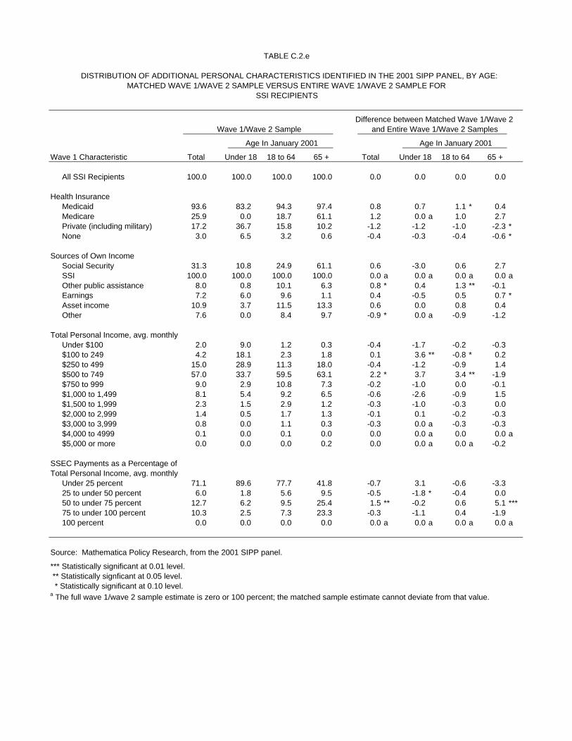
TABLE C.2.e

DISTRIBUTION OF ADDITIONAL PERSONAL CHARACTERISTICS IDENTIFIED IN THE 2001 SIPP PANEL, BY AGE:MATCHED WAVE 1/WAVE 2 SAMPLE VERSUS ENTIRE WAVE 1/WAVE 2 SAMPLE FOR

SSI RECIPIENTS

Difference between Matched Wave 1/Wave 2Wave 1/Wave 2 Sample and Entire Wave 1/Wave 2 Samples

Age In January 2001 Age In January 2001

Wave 1 Characteristic Total Under 18 18 to 64 65 + Total Under 18 18 to 64 65 +

All SSI Recipients 100.0 100.0 100.0 100.0 0.0 0.0 0.0 0.0

Health InsuranceMedicaid 93.6 83.2 94.3 97.4 0.8 0.7 1.1 * 0.4 Medicare 25.9 0.0 18.7 61.1 1.2 0.0 a 1.0 2.7 Private (including military) 17.2 36.7 15.8 10.2 -1.2 -1.2 -1.0 -2.3 *None 3.0 6.5 3.2 0.6 -0.4 -0.3 -0.4 -0.6 *

Sources of Own IncomeSocial Security 31.3 10.8 24.9 61.1 0.6 -3.0 0.6 2.7 SSI 100.0 100.0 100.0 100.0 0.0 a 0.0 a 0.0 a 0.0 aOther public assistance 8.0 0.8 10.1 6.3 0.8 * 0.4 1.3 ** -0.1 Earnings 7.2 6.0 9.6 1.1 0.4 -0.5 0.5 0.7 *Asset income 10.9 3.7 11.5 13.3 0.6 0.0 0.8 0.4 Other 7.6 0.0 8.4 9.7 -0.9 * 0.0 a -0.9 -1.2

Total Personal Income, avg. monthlyUnder $100 2.0 9.0 1.2 0.3 -0.4 -1.7 -0.2 -0.3 $100 to 249 4.2 18.1 2.3 1.8 0.1 3.6 ** -0.8 * 0.2 $250 to 499 15.0 28.9 11.3 18.0 -0.4 -1.2 -0.9 1.4 $500 to 749 57.0 33.7 59.5 63.1 2.2 * 3.7 3.4 ** -1.9 $750 to 999 9.0 2.9 10.8 7.3 -0.2 -1.0 0.0 -0.1 $1,000 to 1,499 8.1 5.4 9.2 6.5 -0.6 -2.6 -0.9 1.5 $1,500 to 1,999 2.3 1.5 2.9 1.2 -0.3 -1.0 -0.3 0.0 $2,000 to 2,999 1.4 0.5 1.7 1.3 -0.1 0.1 -0.2 -0.3 $3,000 to 3,999 0.8 0.0 1.1 0.3 -0.3 0.0 a -0.3 -0.3 $4,000 to 4999 0.1 0.0 0.1 0.0 0.0 0.0 a 0.0 0.0 a$5,000 or more 0.0 0.0 0.0 0.2 0.0 0.0 a 0.0 a -0.2

SSEC Payments as a Percentage ofTotal Personal Income, avg. monthly

Under 25 percent 71.1 89.6 77.7 41.8 -0.7 3.1 -0.6 -3.3 25 to under 50 percent 6.0 1.8 5.6 9.5 -0.5 -1.8 * -0.4 0.0 50 to under 75 percent 12.7 6.2 9.5 25.4 1.5 ** -0.2 0.6 5.1 ***75 to under 100 percent 10.3 2.5 7.3 23.3 -0.3 -1.1 0.4 -1.9 100 percent 0.0 0.0 0.0 0.0 0.0 a 0.0 a 0.0 a 0.0 a

Source: Mathematica Policy Research, from the 2001 SIPP panel.

*** Statistically significant at 0.01 level. ** Statistically signficant at 0.05 level. * Statistically significant at 0.10 level.a The full wave 1/wave 2 sample estimate is zero or 100 percent; the matched sample estimate cannot deviate from that value.

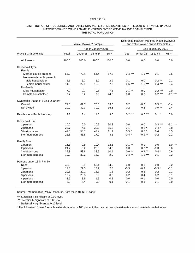
TABLE C.3.a

DISTRIBUTION OF HOUSEHOLD AND FAMILY CHARACTERISTICS IDENTIFIED IN THE 2001 SIPP PANEL, BY AGE:MATCHED WAVE 1/WAVE 2 SAMPLE VERSUS ENTIRE WAVE 1/WAVE 2 SAMPLE FOR

THE TOTAL POPULATION

Difference between Matched Wave 1/Wave 2Wave 1/Wave 2 Sample and Entire Wave 1/Wave 2 Samples

Age In January 2001 Age In January 2001

Wave 1 Characteristic Total Under 18 18 to 64 65 + Total Under 18 18 to 64 65 +

All Persons 100.0 100.0 100.0 100.0 0.0 0.0 0.0 0.0

Household TypeFamily Married couple present 65.2 70.4 64.4 57.8 -0.4 *** -1.5 *** -0.1 0.6 No married couple present Male householder 5.1 5.7 5.2 2.9 -0.1 0.0 -0.2 ** 0.1 Female householder 14.8 22.9 12.8 7.3 0.6 *** 1.5 *** 0.4 *** 0.4 Nonfamily Male householder 7.0 0.7 9.5 7.6 -0.1 ** 0.0 -0.2 *** 0.0 Female householder 7.7 0.2 7.8 24.0 0.0 0.0 0.2 *** -1.1 ***

Ownership Status of Living QuartersOwned 71.0 67.7 70.0 83.5 0.2 -0.2 0.5 ** -0.4 Not owned 29.0 32.3 30.0 16.5 -0.2 0.2 -0.5 ** 0.4

Residence in Public Housing 2.3 3.4 1.8 3.0 0.2 *** 0.5 *** 0.1 * 0.0

Household Size1 person 10.0 0.0 10.2 30.2 0.0 0.0 0.3 *** -1.1 ***2 persons 26.7 4.6 30.3 55.6 -0.1 0.2 * -0.4 * 0.8 *3 to 4 persons 41.6 53.7 42.4 11.1 0.5 * 0.7 * 0.4 0.5 5 or more persons 21.8 41.8 17.0 3.1 -0.4 * -0.9 ** -0.2 -0.2

Family Size1 person 16.1 0.8 19.4 32.1 -0.1 ** -0.1 0.0 -1.0 ***2 persons 24.7 6.2 26.5 54.6 0.0 0.3 ** -0.3 0.6 3 to 4 persons 39.3 53.8 38.9 10.4 0.6 ** 0.9 ** 0.4 * 0.6 *5 or more persons 19.9 39.2 15.2 2.9 -0.4 ** -1.1 *** -0.1 -0.2

Persons under 18 in FamilyNone 46.0 0.9 55.4 94.9 0.0 -0.1 0.0 0.2 1 person 17.8 22.3 18.9 2.5 -0.3 -0.3 -0.3 * -0.1 2 persons 20.5 39.1 16.3 1.6 0.2 0.3 0.2 -0.1 3 persons 10.2 23.3 6.5 0.6 0.2 0.4 0.2 -0.1 4 persons 3.6 8.9 1.9 0.2 0.0 -0.1 0.0 0.0 5 or more persons 2.0 5.4 0.9 0.1 -0.1 -0.3 -0.1 0.0

Source: Mathematica Policy Research, from the 2001 SIPP panel.

*** Statistically significant at 0.01 level. ** Statistically signficant at 0.05 level. * Statistically significant at 0.10 level.a The full wave 1/wave 2 sample estimate is zero or 100 percent; the matched sample estimate cannot deviate from that value.

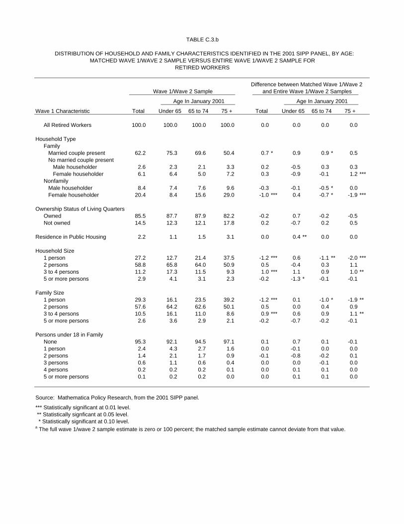
TABLE C.3.b

DISTRIBUTION OF HOUSEHOLD AND FAMILY CHARACTERISTICS IDENTIFIED IN THE 2001 SIPP PANEL, BY AGE:MATCHED WAVE 1/WAVE 2 SAMPLE VERSUS ENTIRE WAVE 1/WAVE 2 SAMPLE FOR

RETIRED WORKERS

Difference between Matched Wave 1/Wave 2Wave 1/Wave 2 Sample and Entire Wave 1/Wave 2 Samples

Age In January 2001 Age In January 2001

Wave 1 Characteristic Total Under 65 65 to 74 75 + Total Under 65 65 to 74 75 +

All Retired Workers 100.0 100.0 100.0 100.0 0.0 0.0 0.0 0.0

Household TypeFamily Married couple present 62.2 75.3 69.6 50.4 0.7 * 0.9 0.9 * 0.5 No married couple present Male householder 2.6 2.3 2.1 3.3 0.2 -0.5 0.3 0.3 Female householder 6.1 6.4 5.0 7.2 0.3 -0.9 -0.1 1.2 ***Nonfamily Male householder 8.4 7.4 7.6 9.6 -0.3 -0.1 -0.5 * 0.0 Female householder 20.4 8.4 15.6 29.0 -1.0 *** 0.4 -0.7 * -1.9 ***

Ownership Status of Living QuartersOwned 85.5 87.7 87.9 82.2 -0.2 0.7 -0.2 -0.5 Not owned 14.5 12.3 12.1 17.8 0.2 -0.7 0.2 0.5

Residence in Public Housing 2.2 1.1 1.5 3.1 0.0 0.4 ** 0.0 0.0

Household Size1 person 27.2 12.7 21.4 37.5 -1.2 *** 0.6 -1.1 ** -2.0 ***2 persons 58.8 65.8 64.0 50.9 0.5 -0.4 0.3 1.1 3 to 4 persons 11.2 17.3 11.5 9.3 1.0 *** 1.1 0.9 1.0 **5 or more persons 2.9 4.1 3.1 2.3 -0.2 -1.3 * -0.1 -0.1

Family Size1 person 29.3 16.1 23.5 39.2 -1.2 *** 0.1 -1.0 * -1.9 **2 persons 57.6 64.2 62.6 50.1 0.5 0.0 0.4 0.9 3 to 4 persons 10.5 16.1 11.0 8.6 0.9 *** 0.6 0.9 1.1 **5 or more persons 2.6 3.6 2.9 2.1 -0.2 -0.7 -0.2 -0.1

Persons under 18 in FamilyNone 95.3 92.1 94.5 97.1 0.1 0.7 0.1 -0.1 1 person 2.4 4.3 2.7 1.6 0.0 -0.1 0.0 0.0 2 persons 1.4 2.1 1.7 0.9 -0.1 -0.8 -0.2 0.1 3 persons 0.6 1.1 0.6 0.4 0.0 0.0 -0.1 0.0 4 persons 0.2 0.2 0.2 0.1 0.0 0.1 0.1 0.0 5 or more persons 0.1 0.2 0.2 0.0 0.0 0.1 0.1 0.0

Source: Mathematica Policy Research, from the 2001 SIPP panel.

*** Statistically significant at 0.01 level. ** Statistically signficant at 0.05 level. * Statistically significant at 0.10 level.a The full wave 1/wave 2 sample estimate is zero or 100 percent; the matched sample estimate cannot deviate from that value.

TABLE C.3.c

DISTRIBUTION OF HOUSEHOLD AND FAMILY CHARACTERISTICS IDENTIFIED IN THE 2001 SIPP PANEL, BY AGE:MATCHED WAVE 1/WAVE 2 SAMPLE VERSUS ENTIRE WAVE 1/WAVE 2 SAMPLE FOR

DISABLED WORKERS

Difference between Matched Wave 1/Wave 2Wave 1/Wave 2 Sample and Entire Wave 1/Wave 2 Samples

Age In January 2001 Age In January 2001

Wave 1 Characteristic Total Under 50 50 to 64 65 + Total Under 50 50 to 64 65 +

All Disabled Workers 100.0 100.0 100.0 100.0 0.0 0.0 0.0 0.0

Household TypeFamily Married couple present 50.0 43.4 55.5 49.5 0.5 1.9 1.2 -2.1 No married couple present Male householder 4.0 4.7 3.4 4.0 -0.5 -0.4 -0.5 -0.7 Female householder 16.8 25.3 13.9 9.6 0.7 -0.5 0.8 1.4 Nonfamily Male householder 12.4 15.3 11.5 9.7 0.3 -0.1 -0.6 2.0 * Female householder 16.4 10.5 15.4 27.2 -0.8 -0.5 -0.9 -0.6

Ownership Status of Living QuartersOwned 65.1 57.5 69.6 68.0 -0.7 2.1 -2.9 * -0.2 Not owned 34.9 42.5 30.4 32.0 0.7 -2.1 2.9 * 0.2

Residence in Public Housing 6.4 6.0 5.5 8.5 0.9 ** 0.2 1.7 *** 0.6

Household Size1 person 23.5 17.7 22.7 33.5 0.0 0.2 -0.2 0.5 2 persons 42.4 32.0 48.1 47.2 -1.0 -3.4 ** 0.9 0.7 3 to 4 persons 25.6 37.0 22.2 15.0 1.1 3.1 ** -0.6 -0.1 5 or more persons 8.5 13.3 7.0 4.3 -0.2 0.1 -0.1 -1.1

Family Size1 person 30.4 28.8 27.9 37.4 -0.8 -1.1 -2.0 1.5 2 persons 38.9 27.6 44.9 44.5 -0.2 -1.9 1.9 -0.1 3 to 4 persons 23.1 31.7 21.1 14.2 0.9 2.6 * -0.6 0.0 5 or more persons 7.6 11.9 6.0 3.9 0.2 0.3 0.7 -1.4

Persons under 18 in FamilyNone 81.1 68.9 84.8 92.5 -0.5 0.5 -1.5 0.8 1 person 9.1 13.0 8.7 4.2 -0.1 -0.3 -0.2 0.0 2 persons 5.5 9.9 3.7 2.4 0.5 0.3 1.3 ** -0.9 3 persons 2.5 5.2 1.5 0.6 0.2 -0.5 0.5 0.4 4 persons 0.9 1.7 0.5 0.3 0.2 0.6 * 0.0 -0.3 5 or more persons 0.8 1.3 0.8 0.0 -0.2 -0.5 -0.1 0.0 a

Source: Mathematica Policy Research, from the 2001 SIPP panel.

*** Statistically significant at 0.01 level. ** Statistically signficant at 0.05 level. * Statistically significant at 0.10 level.a The full wave 1/wave 2 sample estimate is zero or 100 percent; the matched sample estimate cannot deviate from that value.

TABLE C.3.d

DISTRIBUTION OF HOUSEHOLD AND FAMILY CHARACTERISTICS IDENTIFIED IN THE 2001 SIPP PANEL, BY AGE:MATCHED WAVE 1/WAVE 2 SAMPLE VERSUS ENTIRE WAVE 1/WAVE 2 SAMPLE FOR

ALL OTHER SOCIAL SECURITY BENEFICIARIES

Difference between Matched Wave 1/Wave 2Wave 1/Wave 2 Sample and Entire Wave 1/Wave 2 Samples

Age In January 2001 Age In January 2001

Wave 1 Characteristic Total Under 18 18 to 64 65 + Total Under 18 18 to 64 65 +

All Other Beneficiaries 100.0 100.0 100.0 100.0 0.0 0.0 0.0 0.0

Household TypeFamily Married couple present 39.1 54.8 35.6 34.1 0.3 1.1 -2.6 0.1 No married couple present Male householder 4.1 8.6 5.2 2.0 0.8 ** 1.6 * 0.7 0.4 Female householder 20.9 35.9 27.8 13.5 0.5 -2.3 1.3 0.9 Nonfamily Male householder 1.5 0.6 3.5 1.4 -0.1 -0.2 -0.5 0.0 Female householder 34.1 0.1 27.4 48.8 -1.6 * -0.1 0.7 -1.4

Ownership Status of Living QuartersOwned 77.3 69.4 75.6 80.8 -0.9 -1.7 -0.3 -0.3 Not owned 22.7 30.6 24.4 19.2 0.9 1.7 0.3 0.3

Residence in Public Housing 4.2 2.9 5.7 4.4 0.3 0.0 1.7 ** 0.0

Household Size1 person 34.2 0.0 26.3 49.3 -1.8 * 0.0 a 0.6 -1.6 2 persons 31.2 10.5 31.7 38.9 -0.7 -0.5 -2.6 0.5 3 to 4 persons 23.5 54.2 31.0 9.9 1.2 -0.6 0.6 0.8 5 or more persons 11.1 35.3 11.1 1.9 1.3 * 1.1 1.4 0.4

Family Size1 person 36.0 0.7 32.2 50.5 -1.3 0.0 1.5 -1.1 2 persons 31.1 12.1 30.6 38.5 -0.9 -0.6 -2.5 0.2 3 to 4 persons 22.3 53.2 27.2 9.3 1.1 -0.4 -0.2 0.7 5 or more persons 10.5 34.0 9.9 1.7 1.1 * 1.0 1.2 0.2

Persons under 18 in FamilyNone 69.8 0.7 70.0 96.1 -1.9 ** 0.0 0.6 -0.5 1 person 10.5 29.7 16.5 1.7 -0.1 -1.3 -2.1 0.1 2 persons 9.9 34.1 7.0 1.4 0.4 -1.0 0.2 0.2 3 persons 6.4 22.4 5.2 0.5 1.2 ** 2.5 0.8 0.1 4 persons 1.7 6.3 0.7 0.2 0.3 -0.1 0.4 0.2 5 or more persons 1.7 6.7 0.7 0.1 0.1 -0.1 0.1 0.0

Source: Mathematica Policy Research, from the 2001 SIPP panel.

*** Statistically significant at 0.01 level. ** Statistically signficant at 0.05 level. * Statistically significant at 0.10 level.a The full wave 1/wave 2 sample estimate is zero or 100 percent; the matched sample estimate cannot deviate from that value.

TABLE C.3.e

DISTRIBUTION OF HOUSEHOLD AND FAMILY CHARACTERISTICS IDENTIFIED IN THE 2001 SIPP PANEL, BY AGE:MATCHED WAVE 1/WAVE 2 SAMPLE VERSUS ENTIRE WAVE 1/WAVE 2 SAMPLE FOR

SSI RECIPIENTS

Difference between Matched Wave 1/Wave 2Wave 1/Wave 2 Sample and Entire Wave 1/Wave 2 Samples

Age In January 2001 Age In January 2001

Wave 1 Characteristic Total Under 18 18 to 64 65 + Total Under 18 18 to 64 65 +

All SSI Recipients 100.0 100.0 100.0 100.0 0.0 0.0 0.0 0.0

Household TypeFamily Married couple present 34.2 41.1 34.1 30.9 -0.6 0.0 -0.1 -2.1 No married couple present Male householder 6.1 8.7 5.9 5.0 -0.3 -0.8 0.1 -1.3 Female householder 27.5 49.5 26.5 17.7 0.4 1.5 -0.3 1.4 Nonfamily Male householder 11.3 0.6 14.3 8.7 0.9 -0.6 1.2 1.3 Female householder 19.9 0.0 18.0 36.6 -0.4 0.0 a -0.6 0.2

Ownership Status of Living QuartersOwned 42.8 41.5 42.7 43.6 -1.5 -1.6 -0.7 -3.4 Not owned 57.2 58.5 57.3 56.4 1.5 1.6 0.7 3.4

Residence in Public Housing 13.2 9.1 11.8 19.5 0.9 -0.1 0.9 1.2

Household Size1 person 26.2 0.0 24.6 45.5 1.2 0.0 a 1.4 1.7 2 persons 25.8 8.6 28.1 29.1 -1.3 0.8 -2.5 ** 1.3 3 to 4 persons 29.8 50.6 30.1 17.3 0.1 1.5 0.3 -1.5 5 or more persons 18.2 40.8 17.2 8.1 -0.1 -2.4 0.8 -1.6

Family Size1 person 33.8 3.6 35.2 46.8 0.6 0.6 0.2 2.3 2 persons 23.2 10.5 23.4 29.9 -0.3 0.1 -0.6 0.4 3 to 4 persons 27.2 50.5 26.6 15.5 0.0 1.5 -0.2 -0.9 5 or more persons 15.8 35.4 14.7 7.8 -0.2 -2.2 0.6 -1.8

Persons under 18 in FamilyNone 66.3 3.6 71.7 86.2 -0.3 0.6 -1.0 2.3 1 person 13.0 25.4 12.4 7.6 -0.1 -1.3 0.3 -0.6 2 persons 10.5 33.8 8.2 3.9 0.5 5.2 ** 0.1 -1.5 3 persons 5.8 22.7 4.2 1.0 0.1 -2.3 0.7 -0.5 4 persons 3.3 13.1 2.1 1.1 -0.1 -2.0 0.1 0.2 5 or more persons 1.1 1.5 1.4 0.2 -0.1 -0.1 -0.2 0.1

Source: Mathematica Policy Research, from the 2001 SIPP panel.

*** Statistically significant at 0.01 level. ** Statistically signficant at 0.05 level. * Statistically significant at 0.10 level.a The full wave 1/wave 2 sample estimate is zero or 100 percent; the matched sample estimate cannot deviate from that value.

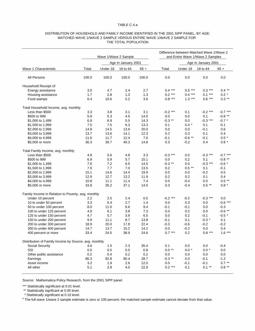
TABLE C.4.a

DISTRIBUTION OF HOUSEHOLD AND FAMILY INCOME IDENTIFIED IN THE 2001 SIPP PANEL, BY AGE:MATCHED WAVE 1/WAVE 2 SAMPLE VERSUS ENTIRE WAVE 1/WAVE 2 SAMPLE FOR

THE TOTAL POPULATION

Difference between Matched Wave 1/Wave 2Wave 1/Wave 2 Sample and Entire Wave 1/Wave 2 Samples

Age In January 2001 Age In January 2001

Wave 1 Characteristic Total Under 18 18 to 64 65 + Total Under 18 18 to 64 65 +

All Persons 100.0 100.0 100.0 100.0 0.0 0.0 0.0 0.0

Household Receipt of:Energy assistance 3.0 4.7 2.4 2.7 0.4 *** 0.5 *** 0.3 *** 0.4 **Housing assistance 1.7 2.8 1.3 1.3 0.2 *** 0.4 *** 0.1 *** 0.2 *Food stamps 6.4 10.6 5.2 3.6 0.8 *** 1.3 *** 0.6 *** 0.3 **

Total Household Income, avg. monthlyLess than $500 3.3 3.8 3.1 3.1 -0.2 *** 0.1 -0.2 *** -0.7 ***$500 to 999 5.9 5.3 4.5 14.5 0.0 0.0 0.1 -0.8 **$1,000 to 1,499 6.9 6.9 5.5 14.3 -0.3 ** 0.0 -0.3 *** -0.7 *$1,500 to 1,999 7.5 7.5 6.3 13.3 0.1 0.4 * 0.1 -0.1 $2,000 to 2,999 14.8 14.5 13.9 20.0 0.0 0.0 -0.1 0.6 $3,000 to 3,999 13.7 13.6 14.1 12.3 0.2 0.3 0.1 0.4 $4,000 to 4,999 11.6 11.7 12.4 7.6 -0.1 -0.6 ** -0.1 0.5 *$5,000 or more 36.3 36.7 40.3 14.8 0.3 -0.2 0.4 0.8 *

Total Family Income, avg. monthlyLess than $500 4.8 5.6 4.8 3.3 -0.3 *** 0.0 -0.3 *** -0.7 ***$500 to 999 6.9 5.9 5.7 15.1 0.0 0.2 0.1 -0.8 **$1,000 to 1,499 7.6 7.2 6.5 14.5 -0.3 ** 0.0 -0.3 *** -0.6 *$1,500 to 1,999 7.9 7.7 7.0 13.5 0.2 0.5 ** 0.1 -0.1 $2,000 to 2,999 15.1 14.6 14.4 19.9 0.0 0.0 -0.2 0.5 $3,000 to 3,999 12.9 12.7 13.2 11.9 0.2 0.2 0.1 0.4 $4,000 to 4,999 10.8 11.1 11.4 7.4 0.0 -0.4 0.0 0.5 **$5,000 or more 33.9 35.2 37.1 14.5 0.3 -0.4 0.5 ** 0.8 *

Family Income in Relation to Poverty, avg. monthlyUnder 10 percent 2.2 2.5 2.4 0.5 -0.2 *** -0.2 -0.3 *** 0.0 10 to under 50 percent 3.3 5.4 2.7 1.4 0.0 0.3 0.0 -0.6 ***50 to under 100 percent 8.0 11.0 6.6 9.4 -0.1 -0.1 0.0 -0.3 100 to under 125 percent 4.8 6.1 3.8 7.3 0.0 0.2 0.0 -0.6 **125 to under 150 percent 4.7 5.7 3.9 6.5 0.0 0.2 -0.1 -0.5 *150 to under 200 percent 9.9 11.1 8.7 13.8 -0.1 0.1 -0.3 * 0.1 200 to under 300 percent 18.9 20.0 17.8 22.4 -0.3 -0.6 -0.2 -0.2 300 to under 400 percent 14.7 13.7 15.2 14.2 0.0 -0.2 0.0 0.4 400 percent or more 33.4 24.5 38.9 24.6 0.7 *** 0.2 0.8 *** 1.6 ***

Distribution of Family Income by Source, avg. monthlySocial Security 4.6 1.5 2.3 35.4 0.1 0.0 0.0 -0.4 SSI 0.5 0.5 0.5 0.8 0.0 ** 0.0 * 0.0 * 0.0 Other public assistance 0.2 0.4 0.2 0.2 0.0 0.0 0.0 0.0 Earnings 86.3 92.8 90.4 28.7 -0.3 ** 0.0 -0.1 -1.2 Asset income 3.2 1.9 2.6 12.0 0.0 -0.1 -0.1 0.7 **All other 5.1 2.8 4.0 22.9 0.2 *** 0.1 0.1 ** 0.8 **

Source: Mathematica Policy Research, from the 2001 SIPP panel.

*** Statistically significant at 0.01 level. ** Statistically signficant at 0.05 level. * Statistically significant at 0.10 level.a The full wave 1/wave 2 sample estimate is zero or 100 percent; the matched sample estimate cannot deviate from that value.

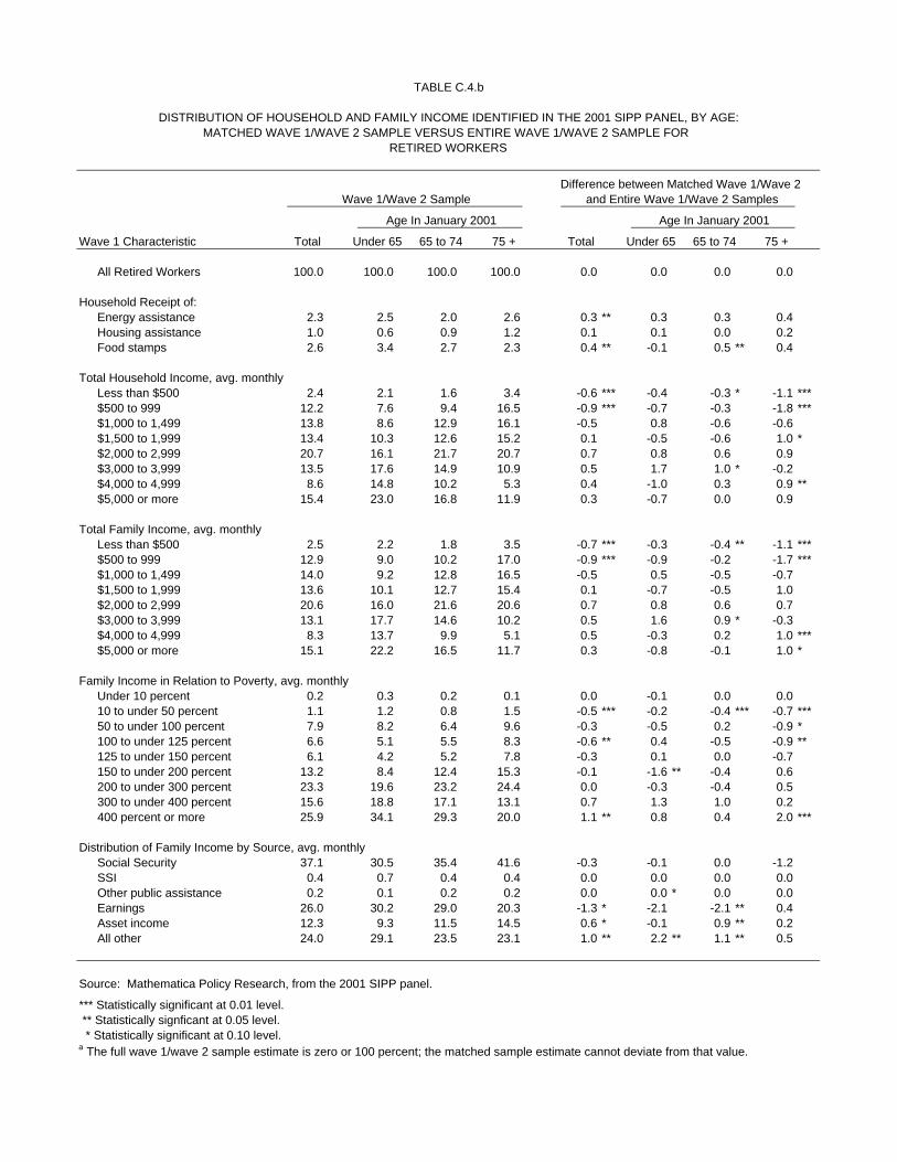
TABLE C.4.b

DISTRIBUTION OF HOUSEHOLD AND FAMILY INCOME IDENTIFIED IN THE 2001 SIPP PANEL, BY AGE:MATCHED WAVE 1/WAVE 2 SAMPLE VERSUS ENTIRE WAVE 1/WAVE 2 SAMPLE FOR

RETIRED WORKERS

Difference between Matched Wave 1/Wave 2Wave 1/Wave 2 Sample and Entire Wave 1/Wave 2 Samples

Age In January 2001 Age In January 2001

Wave 1 Characteristic Total Under 65 65 to 74 75 + Total Under 65 65 to 74 75 +

All Retired Workers 100.0 100.0 100.0 100.0 0.0 0.0 0.0 0.0

Household Receipt of:Energy assistance 2.3 2.5 2.0 2.6 0.3 ** 0.3 0.3 0.4 Housing assistance 1.0 0.6 0.9 1.2 0.1 0.1 0.0 0.2 Food stamps 2.6 3.4 2.7 2.3 0.4 ** -0.1 0.5 ** 0.4

Total Household Income, avg. monthlyLess than $500 2.4 2.1 1.6 3.4 -0.6 *** -0.4 -0.3 * -1.1 ***$500 to 999 12.2 7.6 9.4 16.5 -0.9 *** -0.7 -0.3 -1.8 ***$1,000 to 1,499 13.8 8.6 12.9 16.1 -0.5 0.8 -0.6 -0.6 $1,500 to 1,999 13.4 10.3 12.6 15.2 0.1 -0.5 -0.6 1.0 *$2,000 to 2,999 20.7 16.1 21.7 20.7 0.7 0.8 0.6 0.9 $3,000 to 3,999 13.5 17.6 14.9 10.9 0.5 1.7 1.0 * -0.2 $4,000 to 4,999 8.6 14.8 10.2 5.3 0.4 -1.0 0.3 0.9 **$5,000 or more 15.4 23.0 16.8 11.9 0.3 -0.7 0.0 0.9

Total Family Income, avg. monthlyLess than $500 2.5 2.2 1.8 3.5 -0.7 *** -0.3 -0.4 ** -1.1 ***$500 to 999 12.9 9.0 10.2 17.0 -0.9 *** -0.9 -0.2 -1.7 ***$1,000 to 1,499 14.0 9.2 12.8 16.5 -0.5 0.5 -0.5 -0.7 $1,500 to 1,999 13.6 10.1 12.7 15.4 0.1 -0.7 -0.5 1.0 $2,000 to 2,999 20.6 16.0 21.6 20.6 0.7 0.8 0.6 0.7 $3,000 to 3,999 13.1 17.7 14.6 10.2 0.5 1.6 0.9 * -0.3 $4,000 to 4,999 8.3 13.7 9.9 5.1 0.5 -0.3 0.2 1.0 ***$5,000 or more 15.1 22.2 16.5 11.7 0.3 -0.8 -0.1 1.0 *

Family Income in Relation to Poverty, avg. monthlyUnder 10 percent 0.2 0.3 0.2 0.1 0.0 -0.1 0.0 0.0 10 to under 50 percent 1.1 1.2 0.8 1.5 -0.5 *** -0.2 -0.4 *** -0.7 ***50 to under 100 percent 7.9 8.2 6.4 9.6 -0.3 -0.5 0.2 -0.9 *100 to under 125 percent 6.6 5.1 5.5 8.3 -0.6 ** 0.4 -0.5 -0.9 **125 to under 150 percent 6.1 4.2 5.2 7.8 -0.3 0.1 0.0 -0.7 150 to under 200 percent 13.2 8.4 12.4 15.3 -0.1 -1.6 ** -0.4 0.6 200 to under 300 percent 23.3 19.6 23.2 24.4 0.0 -0.3 -0.4 0.5 300 to under 400 percent 15.6 18.8 17.1 13.1 0.7 1.3 1.0 0.2 400 percent or more 25.9 34.1 29.3 20.0 1.1 ** 0.8 0.4 2.0 ***

Distribution of Family Income by Source, avg. monthlySocial Security 37.1 30.5 35.4 41.6 -0.3 -0.1 0.0 -1.2 SSI 0.4 0.7 0.4 0.4 0.0 0.0 0.0 0.0 Other public assistance 0.2 0.1 0.2 0.2 0.0 0.0 * 0.0 0.0 Earnings 26.0 30.2 29.0 20.3 -1.3 * -2.1 -2.1 ** 0.4 Asset income 12.3 9.3 11.5 14.5 0.6 * -0.1 0.9 ** 0.2 All other 24.0 29.1 23.5 23.1 1.0 ** 2.2 ** 1.1 ** 0.5

Source: Mathematica Policy Research, from the 2001 SIPP panel.

*** Statistically significant at 0.01 level. ** Statistically signficant at 0.05 level. * Statistically significant at 0.10 level.a The full wave 1/wave 2 sample estimate is zero or 100 percent; the matched sample estimate cannot deviate from that value.

TABLE C.4.c

DISTRIBUTION OF HOUSEHOLD AND FAMILY INCOME IDENTIFIED IN THE 2001 SIPP PANEL, BY AGE:MATCHED WAVE 1/WAVE 2 SAMPLE VERSUS ENTIRE WAVE 1/WAVE 2 SAMPLE FOR

DISABLED WORKERS

Difference between Matched Wave 1/Wave 2Wave 1/Wave 2 Sample and Entire Wave 1/Wave 2 Samples

Age In January 2001 Age In January 2001

Wave 1 Characteristic Total Under 50 50 to 64 65 + Total Under 50 50 to 64 65 +

All Disabled Workers 100.0 100.0 100.0 100.0 0.0 0.0 0.0 0.0

Household Receipt of:Energy assistance 9.7 11.6 8.2 9.7 0.6 0.0 1.2 0.5 Housing assistance 4.9 6.5 3.9 4.5 0.6 -0.1 0.9 1.0 Food stamps 15.5 18.7 13.6 14.5 1.5 * -0.3 2.7 *** 1.5

Total Household Income, avg. monthlyLess than $500 2.3 1.8 1.7 4.0 -0.6 ** -0.8 * -0.9 ** 0.2 $500 to 999 20.6 17.3 19.6 27.4 0.5 -1.4 1.5 1.9 $1,000 to 1,499 13.5 12.8 13.0 15.4 -1.0 -0.2 -1.4 -1.4 $1,500 to 1,999 13.9 14.0 14.2 13.0 0.8 2.6 ** 0.8 -2.1 $2,000 to 2,999 16.6 17.0 15.6 17.7 0.4 1.1 -1.6 2.7 *$3,000 to 3,999 12.9 14.2 13.4 10.0 0.0 -0.7 1.0 -1.0 $4,000 to 4,999 9.1 9.1 11.0 5.7 0.9 0.2 1.5 1.1 $5,000 or more 11.1 13.7 11.4 6.7 -1.0 -1.0 -0.9 -1.4

Total Family Income, avg. monthlyLess than $500 2.6 2.5 1.9 4.0 -0.6 ** -0.6 -1.1 ** 0.2 $500 to 999 24.4 23.7 22.6 28.9 -0.1 -1.7 0.0 2.1 $1,000 to 1,499 14.4 15.2 13.2 15.5 -0.6 -0.3 -0.8 -1.0 $1,500 to 1,999 13.2 12.7 13.6 13.2 0.7 2.1 ** 1.1 -2.2 $2,000 to 2,999 15.8 14.8 15.4 17.9 0.8 2.0 * -1.1 2.5 $3,000 to 3,999 11.5 11.9 12.1 9.5 0.0 -0.6 1.1 -0.8 $4,000 to 4,999 8.0 7.9 9.9 4.7 1.0 * 0.6 1.6 * 0.7 $5,000 or more 10.1 11.3 11.2 6.3 -1.2 * -1.6 -0.7 -1.6

Family Income in Relation to Poverty, avg. monthlyUnder 10 percent 0.2 0.2 0.1 0.4 0.0 -0.2 0.1 0.2 10 to under 50 percent 1.4 1.7 1.3 1.3 -0.2 0.1 -0.5 0.0 50 to under 100 percent 21.0 24.3 19.5 18.9 0.6 -0.9 0.0 3.5 **100 to under 125 percent 10.3 9.7 8.4 14.4 -0.3 0.4 0.3 -2.5 125 to under 150 percent 8.4 8.9 7.6 9.4 -0.2 0.2 -0.1 -1.1 150 to under 200 percent 13.5 13.7 13.4 13.6 0.4 0.8 0.3 0.0 200 to under 300 percent 19.4 16.5 22.5 17.7 -0.8 0.2 -2.2 0.7 300 to under 400 percent 12.5 13.9 11.2 13.0 0.2 -0.7 1.2 -0.3 400 percent or more 13.2 11.1 16.0 11.1 0.2 0.2 0.9 -0.4

Distribution of Family Income by Source, avg. monthlySocial Security 38.6 35.8 37.8 45.3 0.7 1.8 -0.1 0.9 SSI 2.8 3.7 2.1 2.5 0.0 -0.2 0.0 0.4 Other public assistance 0.6 0.9 0.5 0.4 0.2 ** 0.3 0.2 * 0.3 **Earnings 41.3 45.8 42.1 31.1 -0.1 -1.3 1.2 -1.7 Asset income 2.5 2.0 2.3 3.8 0.4 0.4 0.2 0.7 All other 14.3 11.9 15.1 16.8 -1.3 -0.9 -1.7 -0.7

Source: Mathematica Policy Research, from the 2001 SIPP panel.

*** Statistically significant at 0.01 level. ** Statistically signficant at 0.05 level. * Statistically significant at 0.10 level.a The full wave 1/wave 2 sample estimate is zero or 100 percent; the matched sample estimate cannot deviate from that value.

TABLE C.4.d

DISTRIBUTION OF HOUSEHOLD AND FAMILY INCOME IDENTIFIED IN THE 2001 SIPP PANEL, BY AGE:MATCHED WAVE 1/WAVE 2 SAMPLE VERSUS ENTIRE WAVE 1/WAVE 2 SAMPLE FOR

ALL OTHER SOCIAL SECURITY BENEFICIARIES

Difference between Matched Wave 1/Wave 2Wave 1/Wave 2 Sample and Entire Wave 1/Wave 2 Samples

Age In January 2001 Age In January 2001

Wave 1 Characteristic Total Under 18 18 to 64 65 + Total Under 18 18 to 64 65 +

All Other Beneficiaries 100.0 100.0 100.0 100.0 0.0 0.0 0.0 0.0

Household Receipt of:Energy assistance 5.1 8.7 5.1 3.8 1.3 *** 2.8 *** 1.9 ** 0.3 Housing assistance 2.5 4.1 2.2 1.9 0.2 0.2 -0.1 0.2 Food stamps 6.4 11.4 8.0 4.0 1.1 ** 1.0 2.1 ** 0.6 *

Total Household Income, avg. monthlyLess than $500 2.6 0.6 2.1 3.4 -0.9 ** 0.0 -0.6 -1.3 **$500 to 999 17.6 7.0 15.0 22.4 0.5 -0.9 2.8 ** 0.9 $1,000 to 1,499 15.1 10.3 10.8 18.0 -1.6 ** 0.3 -0.1 -2.6 **$1,500 to 1,999 12.9 9.1 17.1 13.3 -0.3 0.7 0.1 -0.7 $2,000 to 2,999 16.0 19.6 16.0 14.6 0.5 2.0 -1.4 0.2 $3,000 to 3,999 10.7 15.7 13.3 8.1 0.8 -0.6 3.6 ** 0.4 $4,000 to 4,999 7.5 10.3 8.5 6.1 0.0 0.3 -3.3 *** 0.7 $5,000 or more 17.6 27.4 17.0 14.0 1.1 -1.7 -0.9 2.4 ***

Total Family Income, avg. monthlyLess than $500 3.3 2.4 3.0 3.7 -1.0 *** -0.6 -0.4 -1.4 **$500 to 999 18.2 7.4 16.7 22.7 0.7 -0.6 2.5 * 1.2 $1,000 to 1,499 15.5 10.6 12.5 18.1 -1.8 ** 0.5 -0.4 -2.9 ***$1,500 to 1,999 13.2 9.9 16.8 13.6 -0.3 0.3 -0.4 -0.4 $2,000 to 2,999 15.2 17.8 14.1 14.4 0.8 2.5 -0.4 0.3 $3,000 to 3,999 10.5 15.8 13.4 7.7 0.6 -0.7 3.6 ** 0.2 $4,000 to 4,999 7.1 9.6 7.6 6.0 0.0 0.3 -3.3 *** 0.6 $5,000 or more 17.1 26.4 15.8 13.9 1.0 -1.6 -1.3 2.4 ***

Family Income in Relation to Poverty, avg. monthlyUnder 10 percent 0.2 0.8 0.0 0.1 -0.2 -0.8 0.0 a -0.1 10 to under 50 percent 1.8 3.0 1.8 1.3 -0.6 * -0.4 -0.2 -0.8 **50 to under 100 percent 13.6 14.1 16.2 12.8 1.0 1.4 2.0 0.6 100 to under 125 percent 9.1 8.0 8.9 9.5 0.5 0.6 1.7 * 0.1 125 to under 150 percent 7.9 8.3 5.8 8.3 -0.7 1.2 -0.4 -1.6 **150 to under 200 percent 16.6 15.4 15.4 17.3 -0.8 -1.5 0.6 -0.9 200 to under 300 percent 19.1 18.0 21.5 18.9 -0.2 1.4 -1.4 -0.5 300 to under 400 percent 10.6 13.0 11.4 9.4 -0.6 -1.5 0.6 -0.7 400 percent or more 21.2 19.5 19.1 22.3 1.7 * -0.3 -3.0 3.8 ***

Distribution of Family Income by Source, avg. monthlySocial Security 32.0 25.7 31.5 35.5 -1.3 ** -0.6 0.4 -2.0 **SSI 1.0 1.3 1.8 0.6 0.0 -0.3 0.4 0.0 Other public assistance 0.2 0.2 0.7 0.1 0.0 0.0 -0.4 0.0 Earnings 44.7 62.3 46.7 34.8 1.7 * 0.5 -1.7 2.9 **Asset income 7.9 2.8 4.7 11.5 0.3 0.5 1.5 * 0.0 All other 14.2 7.6 14.6 17.5 -0.6 -0.2 -0.1 -0.9

Source: Mathematica Policy Research, from the 2001 SIPP panel.

*** Statistically significant at 0.01 level. ** Statistically signficant at 0.05 level. * Statistically significant at 0.10 level.a The full wave 1/wave 2 sample estimate is zero or 100 percent; the matched sample estimate cannot deviate from that value.

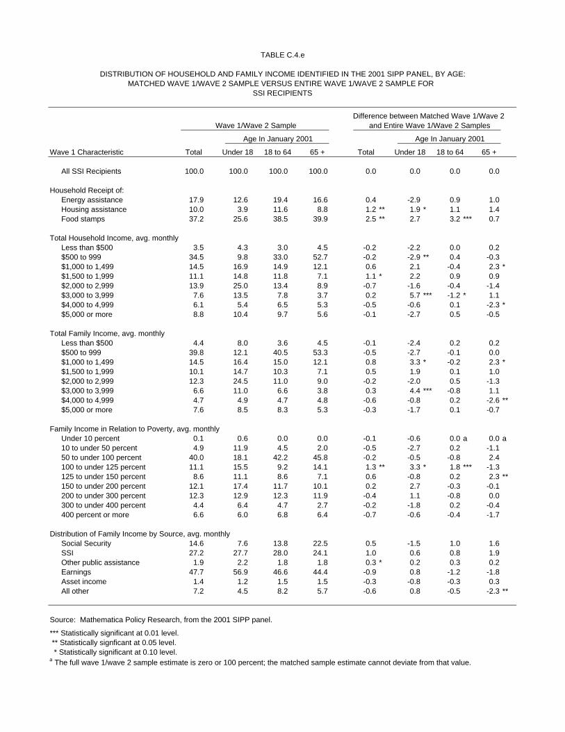
TABLE C.4.e

DISTRIBUTION OF HOUSEHOLD AND FAMILY INCOME IDENTIFIED IN THE 2001 SIPP PANEL, BY AGE:MATCHED WAVE 1/WAVE 2 SAMPLE VERSUS ENTIRE WAVE 1/WAVE 2 SAMPLE FOR

SSI RECIPIENTS

Difference between Matched Wave 1/Wave 2Wave 1/Wave 2 Sample and Entire Wave 1/Wave 2 Samples

Age In January 2001 Age In January 2001

Wave 1 Characteristic Total Under 18 18 to 64 65 + Total Under 18 18 to 64 65 +

All SSI Recipients 100.0 100.0 100.0 100.0 0.0 0.0 0.0 0.0

Household Receipt of:Energy assistance 17.9 12.6 19.4 16.6 0.4 -2.9 0.9 1.0 Housing assistance 10.0 3.9 11.6 8.8 1.2 ** 1.9 * 1.1 1.4 Food stamps 37.2 25.6 38.5 39.9 2.5 ** 2.7 3.2 *** 0.7

Total Household Income, avg. monthlyLess than $500 3.5 4.3 3.0 4.5 -0.2 -2.2 0.0 0.2 $500 to 999 34.5 9.8 33.0 52.7 -0.2 -2.9 ** 0.4 -0.3 $1,000 to 1,499 14.5 16.9 14.9 12.1 0.6 2.1 -0.4 2.3 *$1,500 to 1,999 11.1 14.8 11.8 7.1 1.1 * 2.2 0.9 0.9 $2,000 to 2,999 13.9 25.0 13.4 8.9 -0.7 -1.6 -0.4 -1.4 $3,000 to 3,999 7.6 13.5 7.8 3.7 0.2 5.7 *** -1.2 * 1.1 $4,000 to 4,999 6.1 5.4 6.5 5.3 -0.5 -0.6 0.1 -2.3 *$5,000 or more 8.8 10.4 9.7 5.6 -0.1 -2.7 0.5 -0.5

Total Family Income, avg. monthlyLess than $500 4.4 8.0 3.6 4.5 -0.1 -2.4 0.2 0.2 $500 to 999 39.8 12.1 40.5 53.3 -0.5 -2.7 -0.1 0.0 $1,000 to 1,499 14.5 16.4 15.0 12.1 0.8 3.3 * -0.2 2.3 *$1,500 to 1,999 10.1 14.7 10.3 7.1 0.5 1.9 0.1 1.0 $2,000 to 2,999 12.3 24.5 11.0 9.0 -0.2 -2.0 0.5 -1.3 $3,000 to 3,999 6.6 11.0 6.6 3.8 0.3 4.4 *** -0.8 1.1 $4,000 to 4,999 4.7 4.9 4.7 4.8 -0.6 -0.8 0.2 -2.6 **$5,000 or more 7.6 8.5 8.3 5.3 -0.3 -1.7 0.1 -0.7

Family Income in Relation to Poverty, avg. monthlyUnder 10 percent 0.1 0.6 0.0 0.0 -0.1 -0.6 0.0 a 0.0 a10 to under 50 percent 4.9 11.9 4.5 2.0 -0.5 -2.7 0.2 -1.1 50 to under 100 percent 40.0 18.1 42.2 45.8 -0.2 -0.5 -0.8 2.4 100 to under 125 percent 11.1 15.5 9.2 14.1 1.3 ** 3.3 * 1.8 *** -1.3 125 to under 150 percent 8.6 11.1 8.6 7.1 0.6 -0.8 0.2 2.3 **150 to under 200 percent 12.1 17.4 11.7 10.1 0.2 2.7 -0.3 -0.1 200 to under 300 percent 12.3 12.9 12.3 11.9 -0.4 1.1 -0.8 0.0 300 to under 400 percent 4.4 6.4 4.7 2.7 -0.2 -1.8 0.2 -0.4 400 percent or more 6.6 6.0 6.8 6.4 -0.7 -0.6 -0.4 -1.7

Distribution of Family Income by Source, avg. monthlySocial Security 14.6 7.6 13.8 22.5 0.5 -1.5 1.0 1.6 SSI 27.2 27.7 28.0 24.1 1.0 0.6 0.8 1.9 Other public assistance 1.9 2.2 1.8 1.8 0.3 * 0.2 0.3 0.2 Earnings 47.7 56.9 46.6 44.4 -0.9 0.8 -1.2 -1.8 Asset income 1.4 1.2 1.5 1.5 -0.3 -0.8 -0.3 0.3 All other 7.2 4.5 8.2 5.7 -0.6 0.8 -0.5 -2.3 **

Source: Mathematica Policy Research, from the 2001 SIPP panel.

*** Statistically significant at 0.01 level. ** Statistically signficant at 0.05 level. * Statistically significant at 0.10 level.a The full wave 1/wave 2 sample estimate is zero or 100 percent; the matched sample estimate cannot deviate from that value.

D-1

APPENDIX D

COMPARISON OF DIFFERENCES BETWEEN MATCHED AND ENTIRE WAVE 1/WAVE 2 SAMPLES: 1996 AND 2001 SIPP PANELS

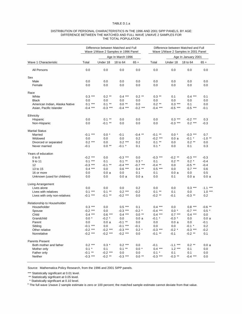
TABLE D.1.a

DISTRIBUTION OF PERSONAL CHARACTERISTICS IN THE 1996 AND 2001 SIPP PANELS, BY AGE:DIFFERENCE BETWEEN THE MATCHED AND FULL WAVE 1/WAVE 2 SAMPLES FOR

THE TOTAL POPULATION

Difference between Matched and Full Difference between Matched and Full Wave 1/Wave 2 Samples in 1996 Panel Wave 1/Wave 2 Samples in 2001 Panel

Age In March 1996 Age In January 2001

Wave 1 Characteristic Total Under 18 18 to 64 65 + Total Under 18 18 to 64 65 +

All Persons 0.0 0.0 0.0 0.0 0.0 0.0 0.0 0.0

SexMale 0.0 0.0 0.0 0.0 0.0 0.0 0.0 0.0 Female 0.0 0.0 0.0 0.0 0.0 0.0 0.0 0.0

RaceWhite 0.3 *** 0.2 ** 0.4 *** 0.2 ** 0.3 ** 0.1 0.4 *** 0.1 Black 0.0 0.0 0.0 0.0 0.0 0.0 0.0 0.0 American Indian, Alaska Native 0.1 *** 0.1 ** 0.0 ** 0.0 0.2 ** 0.3 *** 0.1 0.0 Asian, Pacific Islander -0.4 *** -0.3 *** -0.4 *** -0.2 *** -0.4 *** -0.5 *** -0.5 *** -0.1

EthnicityHispanic 0.0 0.1 ** 0.0 0.0 0.0 0.3 *** -0.2 *** 0.3 Non-Hispanic 0.0 -0.1 ** 0.0 0.0 0.0 -0.3 *** 0.2 *** -0.3

Marital StatusMarried -0.1 *** 0.0 * -0.1 -0.4 ** -0.1 ** 0.0 * -0.3 *** 0.7 Widowed 0.0 0.0 0.0 0.2 -0.2 *** 0.0 a -0.1 * -1.0 **Divorced or separated 0.2 *** 0.0 0.2 *** 0.2 0.1 ** 0.0 0.2 ** 0.0 Never married -0.1 0.0 ** -0.1 * 0.1 0.1 * 0.0 0.1 0.3

Years of education0 to 8 -0.2 *** 0.0 -0.3 *** 0.0 -0.3 *** -0.2 ** -0.3 *** -0.3 9 to 11 0.1 *** 0.1 0.1 ** 0.3 * 0.1 0.2 ** 0.2 * -0.4 12 -0.3 *** -0.1 ** -0.4 *** -0.7 *** -0.4 ** 0.0 -0.5 ** -0.4 13 to 15 0.4 *** 0.0 0.6 *** 0.4 ** 0.5 *** 0.0 0.7 *** 0.6 16 or more 0.0 0.0 a 0.0 0.1 0.1 0.0 a 0.0 0.5 Unknown (used for children) 0.0 0.0 0.0 a 0.0 a 0.0 0.1 0.0 a 0.0 a

Living ArrangementLives alone 0.0 0.0 0.0 0.2 0.0 0.0 0.3 *** -1.1 ***Lives with relatives 0.1 *** 0.1 ** 0.2 *** -0.2 0.1 ** 0.1 0.0 1.0 ***Lives with only non-relatives -0.1 *** -0.1 ** -0.2 *** 0.0 -0.2 ** -0.1 -0.3 ** 0.2

Relationship to HouseholderHouseholder 0.3 *** 0.0 0.5 *** 0.1 0.4 *** 0.0 0.8 *** -0.6 **Spouse -0.2 *** 0.0 -0.3 *** -0.2 * -0.4 *** 0.0 * -0.7 *** 0.5 *Child 0.4 *** 0.6 *** 0.4 *** 0.0 ** 0.4 *** 0.7 *** 0.4 *** 0.0 Grandchild 0.0 * -0.2 * 0.0 0.0 a -0.1 * -0.3 * 0.0 0.0 aParent 0.0 0.0 a -0.1 ** 0.0 0.0 0.0 a 0.0 -0.1 Sibling -0.1 *** 0.0 -0.1 *** -0.1 0.0 0.0 -0.1 * 0.2 Other relative -0.2 *** -0.2 *** -0.3 *** 0.2 * -0.3 *** -0.2 * -0.3 *** -0.2 Nonrelative -0.2 *** -0.2 *** -0.2 *** 0.0 -0.1 ** -0.1 -0.2 ** 0.1

Parents PresentBoth mother and father 0.2 *** 0.3 * 0.2 *** 0.0 -0.1 -1.1 *** 0.2 ** 0.0 aMother only 0.1 * 0.1 0.1 ** 0.0 * 0.4 *** 1.2 *** 0.1 0.0 Father only -0.1 ** -0.2 *** 0.0 0.0 0.1 * 0.1 0.1 0.0 Neither -0.3 *** -0.2 ** -0.3 *** 0.0 ** -0.3 *** -0.3 ** -0.4 *** 0.0

Source: Mathematica Policy Research, from the 1996 and 2001 SIPP panels.

*** Statistically significant at 0.01 level. ** Statistically signficant at 0.05 level. * Statistically significant at 0.10 level.a The full wave 1/wave 2 sample estimate is zero or 100 percent; the matched sample estimate cannot deviate from that value.

TABLE D.1.b

DISTRIBUTION OF PERSONAL CHARACTERISTICS IN THE 1996 AND 2001 SIPP PANELS, BY AGE:DIFFERENCE BETWEEN THE MATCHED AND FULL WAVE 1/WAVE 2 SAMPLES FOR

RETIRED WORKERS

Difference between Matched and Full Difference between Matched and Full Wave 1/Wave 2 Samples in 1996 Panel Wave 1/Wave 2 Samples in 2001 Panel

Age In March 1996 Age In January 2001

Wave 1 Characteristic Total Under 65 65 to 74 75 + Total Under 65 65 to 74 75 +

All Retired Workers 0.0 0.0 0.0 0.0 0.0 0.0 0.0 0.0

SexMale 0.0 -0.2 0.0 0.1 -0.4 -0.2 -0.7 ** 0.0 Female 0.0 0.2 0.0 -0.1 0.4 0.2 0.7 ** 0.0

RaceWhite 0.1 0.7 0.0 0.2 0.2 1.9 * 0.0 0.0 Black -0.1 -0.4 -0.1 0.0 -0.1 -1.2 0.1 0.0 American Indian, Alaska Native 0.0 0.1 ** 0.0 0.0 0.0 0.0 0.0 0.1 Asian, Pacific Islander -0.1 -0.4 0.1 -0.1 -0.1 -0.7 -0.1 0.0

EthnicityHispanic 0.0 -0.2 0.0 0.0 0.1 0.9 -0.2 0.3 Non-Hispanic 0.0 0.2 0.0 0.0 -0.1 -0.9 0.2 -0.3

Marital StatusMarried -0.3 * 1.3 ** 0.2 -1.4 *** 0.8 * 0.7 1.2 ** 0.4 Widowed 0.0 -0.9 ** -0.4 * 0.7 * -0.8 ** -0.3 -1.1 ** -0.8 Divorced or separated 0.1 -0.2 0.0 0.3 * -0.2 -0.1 -0.3 0.0 Never married 0.2 ** -0.2 0.2 0.3 ** 0.2 -0.2 0.1 0.3

Years of education0 to 8 -0.1 0.4 -0.1 -0.2 -0.3 -0.8 0.4 -1.0 *9 to 11 0.3 0.2 0.3 0.3 -0.4 -1.4 -0.5 -0.1 12 -0.7 *** -0.7 -0.8 *** -0.6 -0.5 -1.3 -0.8 0.1 13 to 15 0.4 ** -0.1 0.4 0.5 0.9 ** 2.8 ** 0.6 0.9 *16 or more 0.1 0.2 0.2 -0.1 0.3 0.6 0.3 0.1 Unknown (used for children) 0.0 a 0.0 a 0.0 a 0.0 a 0.0 a 0.0 a 0.0 a 0.0 a

Living ArrangementLives alone 0.1 -1.0 ** -0.1 0.6 * -1.2 *** 0.6 -1.1 ** -2.0 ***Lives with relatives -0.2 0.6 0.1 -0.7 1.2 *** -0.1 1.0 * 1.9 **Lives with only non-relatives 0.1 0.3 * 0.1 0.0 0.0 -0.5 0.0 0.1

Relationship to HouseholderHouseholder -0.1 0.1 0.0 -0.2 -0.6 * 3.5 *** -1.2 *** -0.9 Spouse -0.3 * 0.0 -0.2 -0.4 0.4 -2.3 * 1.4 *** 0.0 Child 0.0 0.0 0.0 ** 0.0 a 0.0 0.4 0.0 0.0 aGrandchild 0.0 a 0.0 a 0.0 a 0.0 a 0.0 0.1 0.0 a 0.0 aParent 0.1 -0.1 0.1 0.3 0.1 -0.1 -0.1 0.5 Sibling 0.0 0.1 -0.1 0.0 0.2 -0.2 0.2 * 0.2 Other relative 0.1 * -0.5 0.2 ** 0.3 * -0.1 -0.4 -0.4 * 0.2 Nonrelative 0.1 0.3 * 0.1 0.1 -0.1 -0.8 0.0 0.1

Parents PresentBoth mother and father 0.0 0.0 0.0 0.0 a 0.0 0.4 0.0 a 0.0 aMother only 0.0 0.1 0.0 0.0 -0.1 -0.2 -0.1 0.0 Father only 0.0 * 0.0 0.0 0.0 a 0.0 0.1 0.0 0.0 aNeither 0.0 * -0.1 -0.1 0.0 0.1 -0.3 0.1 0.0

Source: Mathematica Policy Research, from the 1996 and 2001 SIPP panels.

*** Statistically significant at 0.01 level. ** Statistically signficant at 0.05 level. * Statistically significant at 0.10 level.a The full wave 1/wave 2 sample estimate is zero or 100 percent; the matched sample estimate cannot deviate from that value.

TABLE D.1.c

DISTRIBUTION OF PERSONAL CHARACTERISTICS IN THE 1996 AND 2001 SIPP PANELS, BY AGE:DIFFERENCE BETWEEN THE MATCHED AND FULL WAVE 1/WAVE 2 SAMPLES FOR

DISABLED WORKERS

Difference between Matched and Full Difference between Matched and Full Wave 1/Wave 2 Samples in 1996 Panel Wave 1/Wave 2 Samples in 2001 Panel

Age In March 1996 Age In January 2001

Wave 1 Characteristic Total Under 50 50 to 64 65 + Total Under 50 50 to 64 65 +

All Disabled Workers 0.0 0.0 0.0 0.0 0.0 0.0 0.0 0.0

SexMale -0.5 0.1 -1.5 * -0.4 -0.7 -0.9 -1.2 0.1 Female 0.5 -0.1 1.5 * 0.4 0.7 0.9 1.2 -0.1

RaceWhite -0.4 -0.7 -0.2 -0.1 -1.6 ** -0.8 -1.5 -2.7 Black 0.1 0.4 0.1 -0.4 1.1 1.0 1.2 1.1 American Indian, Alaska Native 0.2 *** 0.1 ** 0.1 0.2 ** 0.3 ** 0.4 ** 0.3 0.3 Asian, Pacific Islander 0.1 0.1 ** 0.0 0.2 * 0.1 -0.5 -0.1 1.3 ***

EthnicityHispanic 0.4 * 0.6 0.7 * -0.2 1.2 ** 0.7 0.9 2.2 *Non-Hispanic -0.4 * -0.6 -0.7 * 0.2 -1.2 ** -0.7 -0.9 -2.2 *

Marital StatusMarried 0.0 -0.1 1.0 0.1 0.3 0.2 1.9 -0.6 Widowed -0.3 0.0 -0.2 0.2 -0.5 -1.1 ** 0.9 -1.5 Divorced or separated -0.4 -0.3 -0.4 -0.6 -0.2 0.1 -0.8 1.1 Never married 0.6 0.3 -0.4 0.3 0.4 0.9 -2.0 * 1.1

Years of education0 to 8 -0.4 -0.8 1.0 -1.3 0.4 1.5 -1.9 3.0 9 to 11 0.0 1.2 ** 0.0 -1.4 -0.7 -1.0 -0.4 -0.6 12 0.0 0.6 -1.7 ** 1.1 -0.2 0.4 -0.2 -1.3 13 to 15 0.4 -0.9 0.7 1.4 *** -0.1 -2.3 2.4 * -1.7 16 or more 0.0 0.0 -0.1 0.1 0.6 1.3 ** 0.1 0.6 Unknown (used for children) 0.0 a 0.0 a 0.0 a 0.0 a 0.0 a 0.0 a 0.0 a 0.0 a

Living ArrangementLives alone -0.3 -0.6 0.0 -0.2 0.0 0.2 -0.2 0.5 Lives with relatives 0.3 0.0 0.7 -0.1 0.8 1.1 2.0 -1.5 Lives with only non-relatives 0.1 0.5 -0.7 0.3 -0.9 -1.3 -1.7 ** 0.9

Relationship to HouseholderHouseholder -0.9 * -0.9 0.2 -1.4 0.4 -2.6 2.6 2.4 Spouse -0.2 -0.3 -0.1 0.2 0.1 1.2 1.1 -2.6 Child 0.3 -0.2 0.0 0.1 0.5 2.1 -1.5 * 0.0 aGrandchild -0.1 -0.2 0.0 a 0.0 a 0.1 0.1 0.0 a 0.0 aParent -0.1 0.0 0.0 -0.4 0.0 0.1 0.4 -0.8 Sibling 0.1 0.1 0.1 -0.2 0.1 0.5 -0.7 0.7 Other relative 0.5 ** 0.6 *** 0.1 0.9 * -0.2 0.1 -0.4 -0.4 Nonrelative 0.5 1.0 * -0.3 0.7 -0.9 * -1.5 -1.6 ** 0.7

Parents PresentBoth mother and father 0.2 0.1 0.0 0.1 0.7 1.7 -0.1 0.0 aMother only 0.2 0.0 0.1 -0.1 0.0 0.1 -0.4 0.0 aFather only 0.0 0.2 -0.2 0.0 a 0.2 0.5 0.1 0.0 aNeither -0.4 -0.3 0.1 0.1 -1.0 -2.3 0.5 0.0 a

Source: Mathematica Policy Research, from the 1996 and 2001 SIPP panels.

*** Statistically significant at 0.01 level. ** Statistically signficant at 0.05 level. * Statistically significant at 0.10 level.a The full wave 1/wave 2 sample estimate is zero or 100 percent; the matched sample estimate cannot deviate from that value.

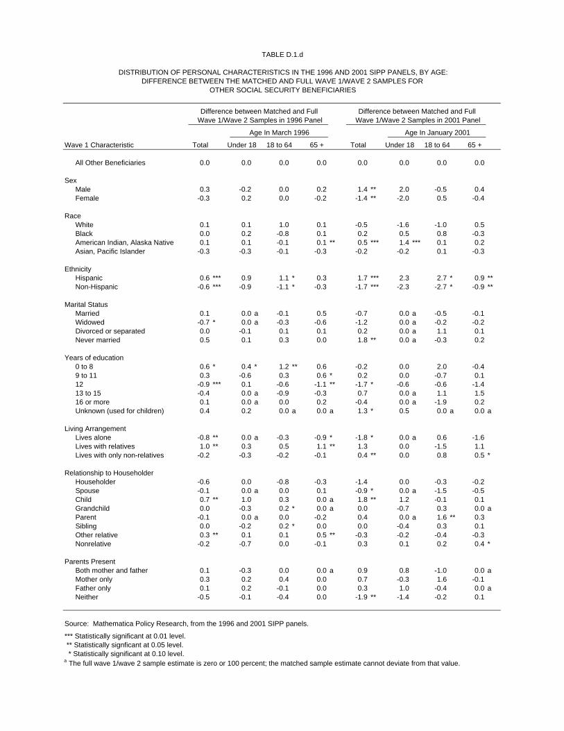
TABLE D.1.d

DISTRIBUTION OF PERSONAL CHARACTERISTICS IN THE 1996 AND 2001 SIPP PANELS, BY AGE:DIFFERENCE BETWEEN THE MATCHED AND FULL WAVE 1/WAVE 2 SAMPLES FOR

OTHER SOCIAL SECURITY BENEFICIARIES

Difference between Matched and Full Difference between Matched and Full Wave 1/Wave 2 Samples in 1996 Panel Wave 1/Wave 2 Samples in 2001 Panel

Age In March 1996 Age In January 2001

Wave 1 Characteristic Total Under 18 18 to 64 65 + Total Under 18 18 to 64 65 +

All Other Beneficiaries 0.0 0.0 0.0 0.0 0.0 0.0 0.0 0.0

SexMale 0.3 -0.2 0.0 0.2 1.4 ** 2.0 -0.5 0.4 Female -0.3 0.2 0.0 -0.2 -1.4 ** -2.0 0.5 -0.4

RaceWhite 0.1 0.1 1.0 0.1 -0.5 -1.6 -1.0 0.5 Black 0.0 0.2 -0.8 0.1 0.2 0.5 0.8 -0.3 American Indian, Alaska Native 0.1 0.1 -0.1 0.1 ** 0.5 *** 1.4 *** 0.1 0.2 Asian, Pacific Islander -0.3 -0.3 -0.1 -0.3 -0.2 -0.2 0.1 -0.3

EthnicityHispanic 0.6 *** 0.9 1.1 * 0.3 1.7 *** 2.3 2.7 * 0.9 **Non-Hispanic -0.6 *** -0.9 -1.1 * -0.3 -1.7 *** -2.3 -2.7 * -0.9 **

Marital StatusMarried 0.1 0.0 a -0.1 0.5 -0.7 0.0 a -0.5 -0.1 Widowed -0.7 * 0.0 a -0.3 -0.6 -1.2 0.0 a -0.2 -0.2 Divorced or separated 0.0 -0.1 0.1 0.1 0.2 0.0 a 1.1 0.1 Never married 0.5 0.1 0.3 0.0 1.8 ** 0.0 a -0.3 0.2

Years of education0 to 8 0.6 * 0.4 * 1.2 ** 0.6 -0.2 0.0 2.0 -0.4 9 to 11 0.3 -0.6 0.3 0.6 * 0.2 0.0 -0.7 0.1 12 -0.9 *** 0.1 -0.6 -1.1 ** -1.7 * -0.6 -0.6 -1.4 13 to 15 -0.4 0.0 a -0.9 -0.3 0.7 0.0 a 1.1 1.5 16 or more 0.1 0.0 a 0.0 0.2 -0.4 0.0 a -1.9 0.2 Unknown (used for children) 0.4 0.2 0.0 a 0.0 a 1.3 * 0.5 0.0 a 0.0 a

Living ArrangementLives alone -0.8 ** 0.0 a -0.3 -0.9 * -1.8 * 0.0 a 0.6 -1.6 Lives with relatives 1.0 ** 0.3 0.5 1.1 ** 1.3 0.0 -1.5 1.1 Lives with only non-relatives -0.2 -0.3 -0.2 -0.1 0.4 ** 0.0 0.8 0.5 *

Relationship to HouseholderHouseholder -0.6 0.0 -0.8 -0.3 -1.4 0.0 -0.3 -0.2 Spouse -0.1 0.0 a 0.0 0.1 -0.9 * 0.0 a -1.5 -0.5 Child 0.7 ** 1.0 0.3 0.0 a 1.8 ** 1.2 -0.1 0.1 Grandchild 0.0 -0.3 0.2 * 0.0 a 0.0 -0.7 0.3 0.0 aParent -0.1 0.0 a 0.0 -0.2 0.4 0.0 a 1.6 ** 0.3 Sibling 0.0 -0.2 0.2 * 0.0 0.0 -0.4 0.3 0.1 Other relative 0.3 ** 0.1 0.1 0.5 ** -0.3 -0.2 -0.4 -0.3 Nonrelative -0.2 -0.7 0.0 -0.1 0.3 0.1 0.2 0.4 *

Parents PresentBoth mother and father 0.1 -0.3 0.0 0.0 a 0.9 0.8 -1.0 0.0 aMother only 0.3 0.2 0.4 0.0 0.7 -0.3 1.6 -0.1 Father only 0.1 0.2 -0.1 0.0 0.3 1.0 -0.4 0.0 aNeither -0.5 -0.1 -0.4 0.0 -1.9 ** -1.4 -0.2 0.1

Source: Mathematica Policy Research, from the 1996 and 2001 SIPP panels.

*** Statistically significant at 0.01 level. ** Statistically signficant at 0.05 level. * Statistically significant at 0.10 level.a The full wave 1/wave 2 sample estimate is zero or 100 percent; the matched sample estimate cannot deviate from that value.

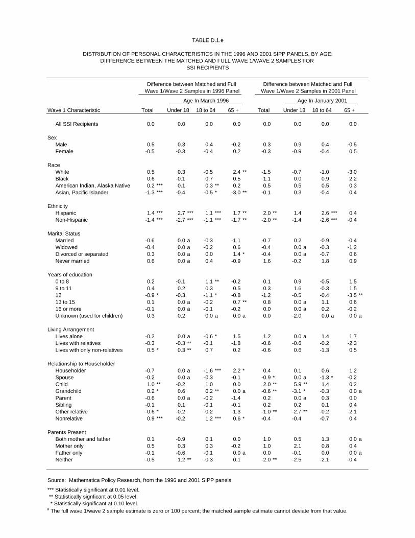
TABLE D.1.e

DISTRIBUTION OF PERSONAL CHARACTERISTICS IN THE 1996 AND 2001 SIPP PANELS, BY AGE:DIFFERENCE BETWEEN THE MATCHED AND FULL WAVE 1/WAVE 2 SAMPLES FOR

SSI RECIPIENTS

Difference between Matched and Full Difference between Matched and Full Wave 1/Wave 2 Samples in 1996 Panel Wave 1/Wave 2 Samples in 2001 Panel

Age In March 1996 Age In January 2001

Wave 1 Characteristic Total Under 18 18 to 64 65 + Total Under 18 18 to 64 65 +

All SSI Recipients 0.0 0.0 0.0 0.0 0.0 0.0 0.0 0.0

SexMale 0.5 0.3 0.4 -0.2 0.3 0.9 0.4 -0.5 Female -0.5 -0.3 -0.4 0.2 -0.3 -0.9 -0.4 0.5

RaceWhite 0.5 0.3 -0.5 2.4 ** -1.5 -0.7 -1.0 -3.0 Black 0.6 -0.1 0.7 0.5 1.1 0.0 0.9 2.2 American Indian, Alaska Native 0.2 *** 0.1 0.3 ** 0.2 0.5 0.5 0.5 0.3 Asian, Pacific Islander -1.3 *** -0.4 -0.5 * -3.0 ** -0.1 0.3 -0.4 0.4

EthnicityHispanic 1.4 *** 2.7 *** 1.1 *** 1.7 ** 2.0 ** 1.4 2.6 *** 0.4 Non-Hispanic -1.4 *** -2.7 *** -1.1 *** -1.7 ** -2.0 ** -1.4 -2.6 *** -0.4

Marital StatusMarried -0.6 0.0 a -0.3 -1.1 -0.7 0.2 -0.9 -0.4 Widowed -0.4 0.0 a -0.2 0.6 -0.4 0.0 a -0.3 -1.2 Divorced or separated 0.3 0.0 a 0.0 1.4 * -0.4 0.0 a -0.7 0.6 Never married 0.6 0.0 a 0.4 -0.9 1.6 -0.2 1.8 0.9

Years of education0 to 8 0.2 -0.1 1.1 ** -0.2 0.1 0.9 -0.5 1.5 9 to 11 0.4 0.2 0.3 0.5 0.3 1.6 -0.3 1.5 12 -0.9 * -0.3 -1.1 * -0.8 -1.2 -0.5 -0.4 -3.5 **13 to 15 0.1 0.0 a -0.2 0.7 ** 0.8 0.0 a 1.1 0.6 16 or more -0.1 0.0 a -0.1 -0.2 0.0 0.0 a 0.2 -0.2 Unknown (used for children) 0.3 0.2 0.0 a 0.0 a 0.0 -2.0 0.0 a 0.0 a

Living ArrangementLives alone -0.2 0.0 a -0.6 * 1.5 1.2 0.0 a 1.4 1.7 Lives with relatives -0.3 -0.3 ** -0.1 -1.8 -0.6 -0.6 -0.2 -2.3 Lives with only non-relatives 0.5 * 0.3 ** 0.7 0.2 -0.6 0.6 -1.3 0.5

Relationship to HouseholderHouseholder -0.7 0.0 a -1.6 *** 2.2 * 0.4 0.1 0.6 1.2 Spouse -0.2 0.0 a -0.3 -0.1 -0.9 * 0.0 a -1.3 * -0.2 Child 1.0 ** -0.2 1.0 0.0 2.0 ** 5.9 ** 1.4 0.2 Grandchild 0.2 * 0.6 0.2 ** 0.0 a -0.6 ** -3.1 * -0.3 0.0 aParent -0.6 0.0 a -0.2 -1.4 0.2 0.0 a 0.3 0.0 Sibling -0.1 0.1 -0.1 -0.1 0.2 0.2 0.1 0.4 Other relative -0.6 * -0.2 -0.2 -1.3 -1.0 ** -2.7 ** -0.2 -2.1 Nonrelative 0.9 *** -0.2 1.2 *** 0.6 * -0.4 -0.4 -0.7 0.4

Parents PresentBoth mother and father 0.1 -0.9 0.1 0.0 1.0 0.5 1.3 0.0 aMother only 0.5 0.3 0.3 -0.2 1.0 2.1 0.8 0.4 Father only -0.1 -0.6 -0.1 0.0 a 0.0 -0.1 0.0 0.0 aNeither -0.5 1.2 ** -0.3 0.1 -2.0 ** -2.5 -2.1 -0.4

Source: Mathematica Policy Research, from the 1996 and 2001 SIPP panels.

*** Statistically significant at 0.01 level. ** Statistically signficant at 0.05 level. * Statistically significant at 0.10 level.a The full wave 1/wave 2 sample estimate is zero or 100 percent; the matched sample estimate cannot deviate from that value.

TABLE D.2.a

DISTRIBUTION OF ADDITIONAL PERSONAL CHARACTERISTICS IN THE 1996 AND 2001 SIPP PANELS, BY AGE:DIFFERENCE BETWEEN THE MATCHED AND FULL WAVE 1/WAVE 2 SAMPLES FOR

THE TOTAL POPULATION

Difference between Matched and Full Difference between Matched and Full Wave 1/Wave 2 Samples in 1996 Panel Wave 1/Wave 2 Samples in 2001 Panel

Age In March 1996 Age In January 2001

Wave 1 Characteristic Total Under 18 18 to 64 65 + Total Under 18 18 to 64 65 +

All Persons 0.0 0.0 0.0 0.0 0.0 0.0 0.0 0.0

Health InsuranceMedicaid 0.4 *** 0.8 *** 0.2 *** 0.3 ** 0.7 *** 1.6 *** 0.5 *** 0.1 Medicare 0.0 0.0 a 0.0 0.4 ** 0.1 * 0.0 a 0.1 0.2 Private (including military) 0.4 *** 0.4 ** 0.3 *** 0.7 *** 0.3 0.1 0.4 * 0.6 None -0.6 *** -1.0 *** -0.5 *** -0.2 *** -0.7 *** -1.0 *** -0.7 *** -0.1

Sources of Own IncomeSocial Security 0.1 *** 0.2 ** 0.1 0.3 ** 0.2 ** 0.2 * 0.1 0.3 SSI 0.1 *** 0.1 *** 0.2 *** 0.1 0.1 *** 0.1 0.1 ** 0.3 Other public assistance 0.0 0.0 0.0 0.1 ** 0.1 *** 0.0 0.1 ** 0.1 Earnings 0.3 *** 0.1 * 0.4 *** 0.4 *** 0.6 *** 0.3 ** 0.7 *** 0.3 Asset income 1.2 *** 0.2 *** 1.5 *** 1.6 *** 1.8 *** 0.6 *** 2.2 *** 2.5 ***Other 0.3 *** 0.0 0.3 *** 1.0 *** 0.5 *** 0.0 0.6 *** 0.8 *

Total Personal Income, avg. monthlyUnder $100 -0.5 *** -0.3 *** -0.6 *** -0.3 *** -0.7 *** -0.5 *** -0.9 *** -0.2 $100 to 249 0.1 * 0.1 ** 0.1 ** -0.2 *** 0.1 * 0.3 *** 0.1 -0.2 $250 to 499 0.1 *** 0.2 *** 0.2 *** -0.2 0.1 0.2 * 0.1 -0.4 $500 to 749 0.0 0.0 0.2 *** -0.6 *** 0.1 0.2 ** 0.1 -0.1 $750 to 999 -0.1 0.0 -0.1 -0.2 -0.2 ** -0.1 0.0 -1.2 ***$1,000 to 1,499 0.1 0.0 ** 0.0 0.5 *** -0.1 -0.1 -0.3 ** 0.5 $1,500 to 1,999 0.0 0.0 0.0 0.4 *** 0.0 0.0 0.0 0.2 $2,000 to 2,999 0.2 *** 0.0 0.2 *** 0.3 *** 0.3 *** 0.0 ** 0.4 *** 0.7 ***$3,000 to 3,999 0.1 ** 0.0 0.1 0.2 *** 0.2 ** 0.0 0.2 ** 0.3 $4,000 to 4999 0.0 0.0 a 0.0 0.1 ** 0.1 ** 0.0 0.1 * 0.2 $5,000 or more 0.0 0.0 a 0.0 0.0 0.1 0.0 0.1 0.1

SSEC Payments as a Percentage ofTotal Personal Income, avg. monthly

Under 25 percent -0.1 ** -0.2 ** -0.1 * 0.0 -0.1 -0.2 -0.1 0.2 25 to under 50 percent 0.1 *** 0.0 *** 0.0 0.5 *** 0.2 *** 0.0 0.0 1.5 ***50 to under 75 percent 0.1 *** 0.0 0.1 *** 0.6 *** 0.1 0.0 0.1 *** 0.1 75 to under 100 percent 0.0 0.0 0.0 0.0 0.0 0.0 0.0 -0.3 100 percent -0.1 *** 0.1 ** 0.0 -1.1 *** -0.2 *** 0.2 * -0.1 ** -1.6 ***

Source: Mathematica Policy Research, from the 1996 and 2001 SIPP panels.

*** Statistically significant at 0.01 level. ** Statistically signficant at 0.05 level. * Statistically significant at 0.10 level.a The full wave 1/wave 2 sample estimate is zero or 100 percent; the matched sample estimate cannot deviate from that value.

TABLE D.2.b

DISTRIBUTION OF ADDITIONAL PERSONAL CHARACTERISTICS IN THE 1996 AND 2001 SIPP PANELS, BY AGE:DIFFERENCE BETWEEN THE MATCHED AND FULL WAVE 1/WAVE 2 SAMPLES FOR

RETIRED WORKERS

Difference between Matched and Full Difference between Matched and Full Wave 1/Wave 2 Samples in 1996 Panel Wave 1/Wave 2 Samples in 2001 Panel

Age In March 1996 Age In January 2001

Wave 1 Characteristic Total Under 65 65 to 74 75 + Total Under 65 65 to 74 75 +

All Retired Workers 0.0 0.0 0.0 0.0 0.0 0.0 0.0 0.0

Health InsuranceMedicaid 0.3 ** 0.2 0.2 0.5 ** 0.1 0.0 0.4 -0.3 Medicare -0.3 ** -2.6 *** 0.0 0.0 a 0.1 -1.7 0.0 0.0 aPrivate (including military) 0.6 *** 0.1 0.5 * 1.0 *** 0.3 -0.7 0.6 0.2 None 0.1 0.6 * 0.0 0.0 a 0.0 0.4 0.0 0.0 a

Sources of Own IncomeSocial Security 0.0 a 0.0 a 0.0 a 0.0 a 0.0 a 0.0 a 0.0 a 0.0 aSSI 0.2 *** 0.2 0.1 0.2 * 0.2 -0.2 0.4 ** 0.0 Other public assistance 0.1 *** 0.1 *** 0.1 ** 0.1 0.1 0.1 0.0 0.2 Earnings 0.2 ** -0.1 0.5 *** 0.0 0.3 2.7 ** 0.0 0.3 Asset income 1.6 *** 0.5 1.5 *** 2.0 *** 2.4 *** 4.8 *** 2.5 *** 1.6 **Other 0.8 *** -0.5 0.8 ** 1.1 ** 1.1 ** 1.8 0.7 1.2

Total Personal Income, avg. monthlyUnder $100 0.0 0.0 0.0 0.0 0.0 -0.2 0.0 -0.1 $100 to 249 -0.1 * 0.2 -0.1 -0.2 -0.2 -0.3 -0.1 -0.3 $250 to 499 -0.1 -0.5 -0.1 -0.1 -0.1 0.8 -0.3 -0.1 $500 to 749 -0.7 *** 0.5 -0.7 *** -1.0 ** -0.2 -0.6 -0.1 -0.2 $750 to 999 -0.2 0.5 -0.2 -0.4 -1.0 *** -0.1 -0.6 -1.7 ***$1,000 to 1,499 0.4 ** 0.2 0.4 * 0.5 0.5 -0.1 0.1 1.0 $1,500 to 1,999 0.3 * -0.8 * 0.4 *** 0.3 0.3 -0.2 0.5 0.2 $2,000 to 2,999 0.3 * -0.3 0.1 0.6 *** 0.5 * -0.3 0.6 0.7 *$3,000 to 3,999 0.2 ** 0.0 0.1 0.3 *** 0.2 1.3 0.0 0.2 $4,000 to 4999 0.1 ** 0.2 0.1 *** 0.0 0.1 -0.5 0.2 0.2 $5,000 or more 0.0 0.1 0.1 -0.1 0.0 0.3 -0.2 0.2

SSEC Payments as a Percentage ofTotal Personal Income, avg. monthly

Under 25 percent 0.3 ** -0.4 0.4 ** 0.3 0.2 -0.8 0.0 0.8 **25 to under 50 percent 0.4 * -0.2 0.7 ** 0.2 1.6 *** 1.1 1.6 *** 1.6 **50 to under 75 percent 0.7 *** 0.9 * 0.4 * 1.1 *** 0.3 2.5 ** 0.5 -0.6 75 to under 100 percent -0.1 0.4 -0.2 0.0 -0.3 0.1 -0.3 -0.6 100 percent -1.3 *** -0.6 -1.3 *** -1.6 *** -1.7 *** -2.9 ** -1.8 *** -1.3 **

Source: Mathematica Policy Research, from the 1996 and 2001 SIPP panels.

*** Statistically significant at 0.01 level. ** Statistically signficant at 0.05 level. * Statistically significant at 0.10 level.a The full wave 1/wave 2 sample estimate is zero or 100 percent; the matched sample estimate cannot deviate from that value.

TABLE D.2.c

DISTRIBUTION OF ADDITIONAL PERSONAL CHARACTERISTICS IN THE 1996 AND 2001 SIPP PANELS, BY AGE:DIFFERENCE BETWEEN THE MATCHED AND FULL WAVE 1/WAVE 2 SAMPLES FOR

DISABLED WORKERS

Difference between Matched and Full Difference between Matched and Full Wave 1/Wave 2 Samples in 1996 Panel Wave 1/Wave 2 Samples in 2001 Panel

Age In March 1996 Age In January 2001

Wave 1 Characteristic Total Under 50 50 to 64 65 + Total Under 50 50 to 64 65 +

All Disabled Workers 0.0 0.0 0.0 0.0 0.0 0.0 0.0 0.0

Health InsuranceMedicaid 1.5 *** 1.8 ** 0.2 1.7 * 2.4 ** 1.6 1.8 3.2 Medicare -0.9 ** -1.0 -0.9 0.0 a 1.6 * 2.1 2.1 0.0 aPrivate (including military) -0.7 -0.9 0.1 -0.4 -0.4 2.0 0.1 -4.0 *None 0.2 0.3 0.2 0.0 a -0.1 0.5 -0.6 0.0 a

Sources of Own IncomeSocial Security 0.0 a 0.0 a 0.0 a 0.0 a 0.0 a 0.0 a 0.0 a 0.0 aSSI 1.4 *** 1.6 ** 0.7 1.1 0.8 0.5 0.4 1.3 Other public assistance -0.1 0.0 -0.5 0.1 0.6 * 0.1 0.4 1.5 ***Earnings 0.1 0.0 0.0 -0.2 1.2 ** 2.4 * 0.4 0.1 Asset income 0.6 0.5 0.9 1.2 1.9 * -0.7 4.1 ** 2.8 Other 0.1 0.5 1.1 -1.0 0.9 0.4 1.5 1.4

Total Personal Income, avg. monthlyUnder $100 0.0 0.0 0.0 a -0.1 -0.2 -0.4 *** -0.2 0.3 $100 to 249 0.1 -0.4 0.3 *** 0.2 0.4 0.8 *** 0.3 0.0 $250 to 499 0.3 0.5 0.2 -0.1 -1.2 * -1.2 -1.4 -0.9 $500 to 749 0.3 0.5 0.3 -0.6 -0.1 -0.6 -0.6 0.5 $750 to 999 -0.2 -0.1 -0.4 0.0 0.7 1.6 0.9 -0.6 $1,000 to 1,499 -0.3 -0.3 -0.4 0.2 -0.7 -0.9 0.5 -2.1 $1,500 to 1,999 0.0 -0.5 0.3 0.6 * 0.4 0.4 0.0 0.9 $2,000 to 2,999 -0.1 0.3 ** -0.4 0.1 1.1 ** 0.5 1.3 1.7 *$3,000 to 3,999 -0.1 0.0 0.0 -0.4 0.2 0.4 -0.1 0.7 *$4,000 to 4999 0.0 * 0.0 0.0 0.0 a -0.2 -0.1 -0.3 -0.2 $5,000 or more 0.0 ** 0.0 0.1 0.0 -0.4 ** -0.5 -0.4 -0.3

SSEC Payments as a Percentage ofTotal Personal Income, avg. monthly

Under 25 percent 0.0 0.1 -0.2 0.0 0.1 0.3 -0.8 0.8 25 to under 50 percent 0.2 0.0 0.1 0.9 0.9 0.9 -0.1 2.5 *50 to under 75 percent 0.8 * 1.7 *** 0.8 -0.3 2.2 ** 1.5 3.4 ** 0.8 75 to under 100 percent 0.2 -0.2 1.0 -0.2 0.5 0.3 1.8 -1.1 100 percent -1.3 ** -1.6 ** -1.7 ** -0.4 -3.6 *** -3.0 * -4.3 ** -2.9

Source: Mathematica Policy Research, from the 1996 and 2001 SIPP panels.

*** Statistically significant at 0.01 level. ** Statistically signficant at 0.05 level. * Statistically significant at 0.10 level.a The full wave 1/wave 2 sample estimate is zero or 100 percent; the matched sample estimate cannot deviate from that value.

TABLE D.2.d

DISTRIBUTION OF ADDITIONAL PERSONAL CHARACTERISTICS IN THE 1996 AND 2001 SIPP PANELS, BY AGE:DIFFERENCE BETWEEN THE MATCHED AND FULL WAVE 1/WAVE 2 SAMPLES FOR

ALL OTHER SOCIAL SECURITY BENEFICIARIES

Difference between Matched and Full Difference between Matched and Full Wave 1/Wave 2 Samples in 1996 Panel Wave 1/Wave 2 Samples in 2001 Panel

Age In March 1996 Age In January 2001

Wave 1 Characteristic Total Under 18 18 to 64 65 + Total Under 18 18 to 64 65 +

All Other Beneficiaries 0.0 0.0 0.0 0.0 0.0 0.0 0.0 0.0

Health InsuranceMedicaid 0.8 *** 0.4 1.7 ** 0.6 ** 1.4 * 1.2 2.7 * 0.3 Medicare -0.3 0.0 a -0.1 0.0 a -1.9 ** 0.0 a 0.1 0.0 aPrivate (including military) -0.7 ** -1.7 * -0.5 -0.2 0.0 0.6 -4.1 * 1.4 None 0.4 ** 1.2 0.3 0.0 a 0.1 -1.9 1.6 0.0 a

Sources of Own IncomeSocial Security 0.0 a 0.0 a 0.0 a 0.0 a 0.0 a 0.0 a 0.0 a 0.0 aSSI 0.3 0.0 0.8 * 0.2 0.3 -1.1 1.3 0.5 Other public assistance 0.1 ** 0.0 a 0.3 0.2 *** 0.0 0.0 a -0.1 0.0 Earnings 0.4 * 0.1 1.2 0.4 0.5 -0.3 -2.0 1.6 **Asset income 0.4 -0.2 0.9 0.9 * 0.9 1.6 * 2.3 1.9 Other 0.5 * 0.1 -0.1 1.1 ** -1.4 * -0.2 0.0 -1.3

Total Personal Income, avg. monthlyUnder $100 0.1 0.4 0.1 -0.1 0.1 -0.4 0.6 -0.1 $100 to 249 -0.1 -0.4 0.0 -0.2 0.7 1.6 0.1 -0.2 $250 to 499 -0.3 0.9 -0.7 -0.8 * -0.3 1.8 -1.2 -1.5 *$500 to 749 -0.3 -1.4 * -0.5 0.2 1.1 0.4 0.0 1.7 *$750 to 999 -0.2 0.6 ** -0.5 -0.4 -1.5 ** -2.1 ** 0.6 -1.5 *$1,000 to 1,499 0.4 * -0.1 1.4 ** 0.6 -1.3 * -1.4 -1.1 -0.9 $1,500 to 1,999 0.1 0.0 0.2 0.2 0.0 0.0 -0.1 0.3 $2,000 to 2,999 0.4 ** 0.0 a 0.3 0.6 ** 0.3 0.1 0.6 0.5 $3,000 to 3,999 0.0 0.0 a -0.3 0.1 0.5 * 0.0 a 0.4 0.8 *$4,000 to 4999 0.0 0.0 a -0.2 0.0 0.3 0.0 a 0.5 * 0.4 $5,000 or more 0.0 0.0 a 0.1 ** -0.1 0.1 0.0 a -0.3 0.4

SSEC Payments as a Percentage ofTotal Personal Income, avg. monthly

Under 25 percent 0.2 0.0 -0.1 0.4 0.2 0.3 * 0.1 0.4 25 to under 50 percent 0.5 * 0.3 *** 1.8 *** 0.4 0.3 -0.2 0.2 1.0 50 to under 75 percent 0.2 0.0 0.6 0.3 -0.6 -0.3 -0.7 -0.3 75 to under 100 percent -0.3 -0.3 -1.6 0.2 0.0 0.6 0.1 0.5 100 percent -0.5 -0.1 -0.8 -1.2 *** 0.1 -0.4 0.3 -1.5

Source: Mathematica Policy Research, from the 1996 and 2001 SIPP panels.

*** Statistically significant at 0.01 level. ** Statistically signficant at 0.05 level. * Statistically significant at 0.10 level.a The full wave 1/wave 2 sample estimate is zero or 100 percent; the matched sample estimate cannot deviate from that value.

TABLE D.2.e

DISTRIBUTION OF ADDITIONAL PERSONAL CHARACTERISTICS IN THE 1996 AND 2001 SIPP PANELS, BY AGE:DIFFERENCE BETWEEN THE MATCHED AND FULL WAVE 1/WAVE 2 SAMPLES FOR

SSI RECIPIENTS

Difference between Matched and Full Difference between Matched and Full Wave 1/Wave 2 Samples in 1996 Panel Wave 1/Wave 2 Samples in 2001 Panel

Age In March 1996 Age In January 2001

Wave 1 Characteristic Total Under 18 18 to 64 65 + Total Under 18 18 to 64 65 +

All SSI Recipients 0.0 0.0 0.0 0.0 0.0 0.0 0.0 0.0

Health InsuranceMedicaid 0.3 1.0 0.1 0.6 0.8 0.7 1.1 * 0.4 Medicare 0.3 0.0 a 0.2 2.8 ** 1.2 0.0 a 1.0 2.7 Private (including military) -0.5 -0.9 -0.5 -0.7 -1.2 -1.2 -1.0 -2.3 *None -0.1 -0.7 -0.1 0.1 -0.4 -0.3 -0.4 -0.6 *

Sources of Own IncomeSocial Security 0.7 -0.3 0.6 3.0 ** 0.6 -3.0 0.6 2.7 SSI 0.0 a 0.0 a 0.0 a 0.0 a 0.0 a 0.0 a 0.0 a 0.0 aOther public assistance 0.3 -0.3 0.1 0.8 * 0.8 * 0.4 1.3 ** -0.1 Earnings 0.2 -0.3 0.4 0.0 0.4 -0.5 0.5 0.7 *Asset income -0.2 0.1 -0.1 -0.4 0.6 0.0 0.8 0.4 Other -0.1 0.1 -0.2 0.3 -0.9 * 0.0 a -0.9 -1.2

Total Personal Income, avg. monthlyUnder $100 0.1 -0.4 0.1 0.1 -0.4 -1.7 -0.2 -0.3 $100 to 249 -0.2 -0.6 0.2 -0.8 0.1 3.6 ** -0.8 * 0.2 $250 to 499 0.2 0.5 0.2 0.0 -0.4 -1.2 -0.9 1.4 $500 to 749 -0.1 -0.1 0.0 0.2 2.2 * 3.7 3.4 ** -1.9 $750 to 999 0.3 0.5 ** 0.3 0.2 -0.2 -1.0 0.0 -0.1 $1,000 to 1,499 0.0 0.0 -0.2 0.2 -0.6 -2.6 -0.9 1.5 $1,500 to 1,999 -0.1 0.0 -0.3 0.1 * -0.3 -1.0 -0.3 0.0 $2,000 to 2,999 -0.1 0.0 a -0.2 -0.1 -0.1 0.1 -0.2 -0.3 $3,000 to 3,999 0.0 ** 0.0 a 0.0 * 0.0 -0.3 0.0 a -0.3 -0.3 $4,000 to 4999 0.0 0.0 a 0.0 0.0 a 0.0 0.0 a 0.0 0.0 a$5,000 or more 0.0 0.0 a 0.0 0.0 a 0.0 0.0 a 0.0 a -0.2

SSEC Payments as a Percentage ofTotal Personal Income, avg. monthly

Under 25 percent -0.6 0.4 -0.6 -3.0 ** -0.7 3.1 -0.6 -3.3 25 to under 50 percent 0.2 0.3 0.1 0.9 * -0.5 -1.8 * -0.4 0.0 50 to under 75 percent 0.6 * -0.9 0.7 ** 1.9 ** 1.5 ** -0.2 0.6 5.1 ***75 to under 100 percent -0.2 0.2 -0.2 0.2 -0.3 -1.1 0.4 -1.9 100 percent 0.0 a 0.0 a 0.0 a 0.0 a 0.0 a 0.0 a 0.0 a 0.0 a

Source: Mathematica Policy Research, from the 1996 and 2001 SIPP panels.

*** Statistically significant at 0.01 level. ** Statistically signficant at 0.05 level. * Statistically significant at 0.10 level.a The full wave 1/wave 2 sample estimate is zero or 100 percent; the matched sample estimate cannot deviate from that value.

TABLE D.3.a

DISTRIBUTION OF HOUSEHOLD AND FAMILY CHARACTERISTICS IN THE 1996 AND 2001 SIPP PANELS, BY AGE:DIFFERENCE BETWEEN THE MATCHED AND FULL WAVE 1/WAVE 2 SAMPLES FOR

THE TOTAL POPULATION

Difference between Matched and Full Difference between Matched and Full Wave 1/Wave 2 Samples in 1996 Panel Wave 1/Wave 2 Samples in 2001 Panel

Age In March 1996 Age In January 2001

Wave 1 Characteristic Total Under 18 18 to 64 65 + Total Under 18 18 to 64 65 +

All Persons 0.0 0.0 0.0 0.0 0.0 0.0 0.0 0.0

Household TypeFamily Married couple present 0.2 ** 0.1 0.2 *** -0.2 -0.4 *** -1.5 *** -0.1 0.6 No married couple present Male householder -0.2 *** -0.2 *** -0.2 *** 0.0 -0.1 0.0 -0.2 ** 0.1 Female householder 0.1 ** 0.3 0.1 * 0.0 0.6 *** 1.5 *** 0.4 *** 0.4 Nonfamily Male householder -0.1 *** -0.1 *** -0.3 *** 0.4 *** -0.1 ** 0.0 -0.2 *** 0.0 Female householder 0.0 0.0 0.1 ** -0.2 0.0 0.0 0.2 *** -1.1 ***

Ownership Status of Living QuartersOwned 0.4 *** 0.2 0.6 *** -0.1 0.2 -0.2 0.5 ** -0.4 Not owned -0.4 *** -0.2 -0.6 *** 0.1 -0.2 0.2 -0.5 ** 0.4

Residence in Public Housing 0.1 *** 0.2 ** 0.1 * 0.2 *** 0.2 *** 0.5 *** 0.1 * 0.0

Household Size1 person 0.0 0.0 0.0 0.2 0.0 0.0 0.3 *** -1.1 ***2 persons 0.1 0.1 0.0 0.0 -0.1 0.2 * -0.4 * 0.8 *3 to 4 persons 0.1 0.1 0.1 0.0 0.5 * 0.7 * 0.4 0.5 5 or more persons -0.1 -0.2 -0.1 -0.2 * -0.4 * -0.9 ** -0.2 -0.2

Family Size1 person -0.1 *** -0.1 ** -0.2 *** 0.2 -0.1 ** -0.1 0.0 -1.0 ***2 persons 0.0 0.0 0.0 0.0 0.0 0.3 ** -0.3 0.6 3 to 4 persons 0.2 ** 0.3 0.2 ** 0.0 0.6 ** 0.9 ** 0.4 * 0.6 *5 or more persons -0.1 -0.2 0.0 -0.2 * -0.4 ** -1.1 *** -0.1 -0.2

Persons under 18 in FamilyNone -0.3 *** -0.1 ** -0.4 *** 0.0 0.0 -0.1 0.0 0.2 1 person 0.1 -0.2 * 0.2 ** 0.0 -0.3 -0.3 -0.3 * -0.1 2 persons 0.1 0.1 0.1 0.0 0.2 0.3 0.2 -0.1 3 persons 0.1 0.2 0.1 0.0 0.2 0.4 0.2 -0.1 4 persons 0.0 0.0 0.1 0.0 0.0 -0.1 0.0 0.0 5 or more persons 0.0 0.0 0.0 0.0 -0.1 -0.3 -0.1 0.0

Source: Mathematica Policy Research, from the 1996 and 2001 SIPP panels.

*** Statistically significant at 0.01 level. ** Statistically signficant at 0.05 level. * Statistically significant at 0.10 level.a The full wave 1/wave 2 sample estimate is zero or 100 percent; the matched sample estimate cannot deviate from that value.

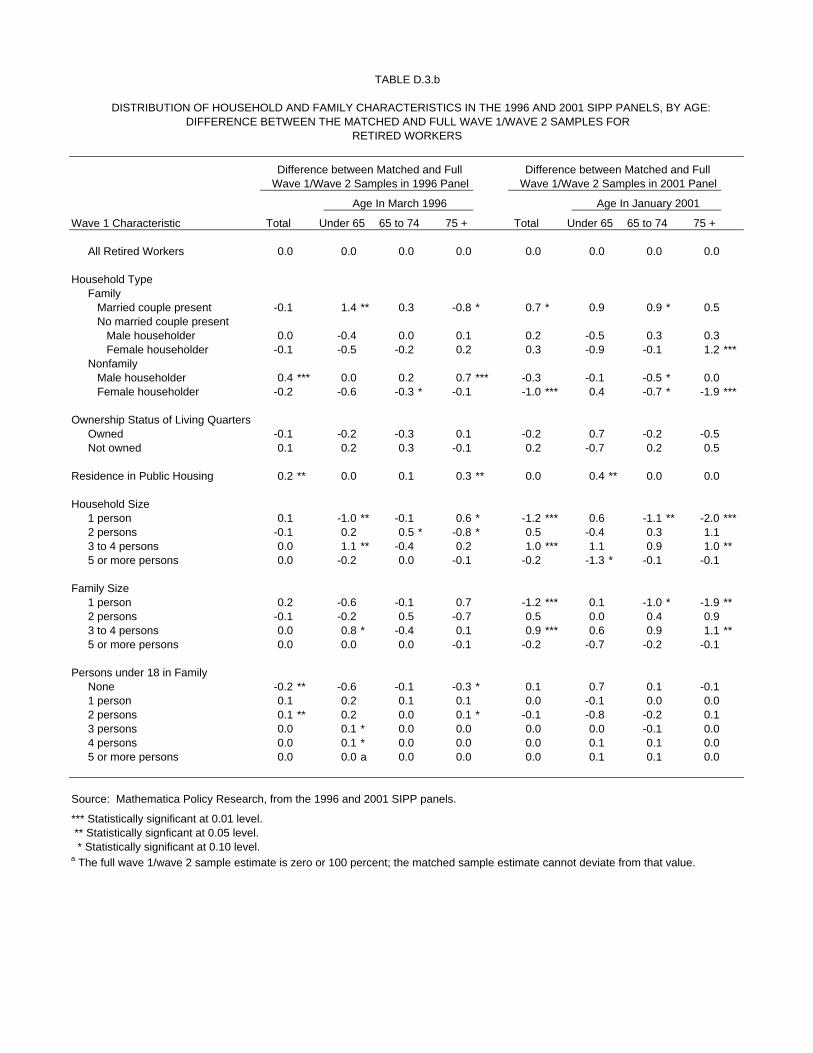
TABLE D.3.b

DISTRIBUTION OF HOUSEHOLD AND FAMILY CHARACTERISTICS IN THE 1996 AND 2001 SIPP PANELS, BY AGE:DIFFERENCE BETWEEN THE MATCHED AND FULL WAVE 1/WAVE 2 SAMPLES FOR

RETIRED WORKERS

Difference between Matched and Full Difference between Matched and Full Wave 1/Wave 2 Samples in 1996 Panel Wave 1/Wave 2 Samples in 2001 Panel

Age In March 1996 Age In January 2001

Wave 1 Characteristic Total Under 65 65 to 74 75 + Total Under 65 65 to 74 75 +

All Retired Workers 0.0 0.0 0.0 0.0 0.0 0.0 0.0 0.0

Household TypeFamily Married couple present -0.1 1.4 ** 0.3 -0.8 * 0.7 * 0.9 0.9 * 0.5 No married couple present Male householder 0.0 -0.4 0.0 0.1 0.2 -0.5 0.3 0.3 Female householder -0.1 -0.5 -0.2 0.2 0.3 -0.9 -0.1 1.2 ***Nonfamily Male householder 0.4 *** 0.0 0.2 0.7 *** -0.3 -0.1 -0.5 * 0.0 Female householder -0.2 -0.6 -0.3 * -0.1 -1.0 *** 0.4 -0.7 * -1.9 ***

Ownership Status of Living QuartersOwned -0.1 -0.2 -0.3 0.1 -0.2 0.7 -0.2 -0.5 Not owned 0.1 0.2 0.3 -0.1 0.2 -0.7 0.2 0.5

Residence in Public Housing 0.2 ** 0.0 0.1 0.3 ** 0.0 0.4 ** 0.0 0.0

Household Size1 person 0.1 -1.0 ** -0.1 0.6 * -1.2 *** 0.6 -1.1 ** -2.0 ***2 persons -0.1 0.2 0.5 * -0.8 * 0.5 -0.4 0.3 1.1 3 to 4 persons 0.0 1.1 ** -0.4 0.2 1.0 *** 1.1 0.9 1.0 **5 or more persons 0.0 -0.2 0.0 -0.1 -0.2 -1.3 * -0.1 -0.1

Family Size1 person 0.2 -0.6 -0.1 0.7 -1.2 *** 0.1 -1.0 * -1.9 **2 persons -0.1 -0.2 0.5 -0.7 0.5 0.0 0.4 0.9 3 to 4 persons 0.0 0.8 * -0.4 0.1 0.9 *** 0.6 0.9 1.1 **5 or more persons 0.0 0.0 0.0 -0.1 -0.2 -0.7 -0.2 -0.1

Persons under 18 in FamilyNone -0.2 ** -0.6 -0.1 -0.3 * 0.1 0.7 0.1 -0.1 1 person 0.1 0.2 0.1 0.1 0.0 -0.1 0.0 0.0 2 persons 0.1 ** 0.2 0.0 0.1 * -0.1 -0.8 -0.2 0.1 3 persons 0.0 0.1 * 0.0 0.0 0.0 0.0 -0.1 0.0 4 persons 0.0 0.1 * 0.0 0.0 0.0 0.1 0.1 0.0 5 or more persons 0.0 0.0 a 0.0 0.0 0.0 0.1 0.1 0.0

Source: Mathematica Policy Research, from the 1996 and 2001 SIPP panels.

*** Statistically significant at 0.01 level. ** Statistically signficant at 0.05 level. * Statistically significant at 0.10 level.a The full wave 1/wave 2 sample estimate is zero or 100 percent; the matched sample estimate cannot deviate from that value.

TABLE D.3.c

DISTRIBUTION OF HOUSEHOLD AND FAMILY CHARACTERISTICS IN THE 1996 AND 2001 SIPP PANELS, BY AGE:DIFFERENCE BETWEEN THE MATCHED AND FULL WAVE 1/WAVE 2 SAMPLES FOR

DISABLED WORKERS

Difference between Matched and Full Difference between Matched and Full Wave 1/Wave 2 Samples in 1996 Panel Wave 1/Wave 2 Samples in 2001 Panel

Age In March 1996 Age In January 2001

Wave 1 Characteristic Total Under 50 50 to 64 65 + Total Under 50 50 to 64 65 +

All Disabled Workers 0.0 0.0 0.0 0.0 0.0 0.0 0.0 0.0

Household TypeFamily Married couple present 0.6 -0.1 1.2 1.5 0.5 1.9 1.2 -2.1 No married couple present Male householder 0.0 -0.2 -0.1 0.1 -0.5 -0.4 -0.5 -0.7 Female householder 0.0 0.9 -0.3 -1.2 0.7 -0.5 0.8 1.4 Nonfamily Male householder -0.6 * -0.4 -1.2 * -0.3 0.3 -0.1 -0.6 2.0 * Female householder -0.1 -0.3 0.6 -0.3 -0.8 -0.5 -0.9 -0.6

Ownership Status of Living QuartersOwned -0.4 -0.9 0.3 0.5 -0.7 2.1 -2.9 * -0.2 Not owned 0.4 0.9 -0.3 -0.5 0.7 -2.1 2.9 * 0.2

Residence in Public Housing 0.6 *** 0.6 * 0.4 0.8 ** 0.9 ** 0.2 1.7 *** 0.6

Household Size1 person -0.3 -0.6 0.0 -0.2 0.0 0.2 -0.2 0.5 2 persons 0.0 0.9 -0.1 0.1 -1.0 -3.4 ** 0.9 0.7 3 to 4 persons 0.1 -1.5 * 0.4 0.6 1.1 3.1 ** -0.6 -0.1 5 or more persons 0.3 1.2 ** -0.4 -0.5 -0.2 0.1 -0.1 -1.1

Family Size1 person -0.3 0.0 -0.7 0.1 -0.8 -1.1 -2.0 1.5 2 persons 0.0 0.6 0.5 -0.3 -0.2 -1.9 1.9 -0.1 3 to 4 persons 0.3 -1.3 0.7 0.8 0.9 2.6 * -0.6 0.0 5 or more persons 0.0 0.7 -0.4 -0.6 0.2 0.3 0.7 -1.4

Persons under 18 in FamilyNone -0.3 -1.0 0.3 1.1 -0.5 0.5 -1.5 0.8 1 person 0.3 0.6 0.2 -0.4 -0.1 -0.3 -0.2 0.0 2 persons 0.3 * 0.5 0.1 0.0 0.5 0.3 1.3 ** -0.9 3 persons -0.5 ** -0.3 -0.5 * -0.8 0.2 -0.5 0.5 0.4 4 persons 0.0 0.0 -0.1 0.2 * 0.2 0.6 * 0.0 -0.3 5 or more persons 0.0 0.1 0.0 -0.1 -0.2 -0.5 -0.1 0.0 a

Source: Mathematica Policy Research, from the 1996 and 2001 SIPP panels.

*** Statistically significant at 0.01 level. ** Statistically signficant at 0.05 level. * Statistically significant at 0.10 level.a The full wave 1/wave 2 sample estimate is zero or 100 percent; the matched sample estimate cannot deviate from that value.

TABLE D.3.d

DISTRIBUTION OF HOUSEHOLD AND FAMILY CHARACTERISTICS IN THE 1996 AND 2001 SIPP PANELS, BY AGE:DIFFERENCE BETWEEN THE MATCHED AND FULL WAVE 1/WAVE 2 SAMPLES FOR

ALL OTHER SOCIAL SECURITY BENEFICIARIES

Difference between Matched and Full Difference between Matched and Full Wave 1/Wave 2 Samples in 1996 Panel Wave 1/Wave 2 Samples in 2001 Panel

Age In March 1996 Age In January 2001

Wave 1 Characteristic Total Under 18 18 to 64 65 + Total Under 18 18 to 64 65 +

All Other Beneficiaries 0.0 0.0 0.0 0.0 0.0 0.0 0.0 0.0

Household TypeFamily Married couple present 0.3 -1.2 0.1 0.8 * 0.3 1.1 -2.6 0.1 No married couple present Male householder 0.0 0.0 0.5 * -0.1 0.8 ** 1.6 * 0.7 0.4 Female householder 0.6 * 1.2 -0.4 0.3 0.5 -2.3 1.3 0.9 Nonfamily Male householder 0.0 0.0 -0.2 0.2 -0.1 -0.2 -0.5 0.0 Female householder -0.9 ** 0.0 0.0 -1.2 ** -1.6 * -0.1 0.7 -1.4

Ownership Status of Living QuartersOwned -1.0 *** -1.6 ** -1.1 -0.5 -0.9 -1.7 -0.3 -0.3 Not owned 1.0 *** 1.6 ** 1.1 0.5 0.9 1.7 0.3 0.3

Residence in Public Housing 0.1 0.0 -0.7 0.3 * 0.3 0.0 1.7 ** 0.0

Household Size1 person -0.8 ** 0.0 a -0.3 -0.9 * -1.8 * 0.0 a 0.6 -1.6 2 persons 0.1 0.8 ** -0.3 0.1 -0.7 -0.5 -2.6 0.5 3 to 4 persons 0.6 -0.1 0.3 0.6 * 1.2 -0.6 0.6 0.8 5 or more persons 0.1 -0.7 0.3 0.1 1.3 * 1.1 1.4 0.4

Family Size1 person -1.0 ** -0.3 -0.5 -1.1 ** -1.3 0.0 1.5 -1.1 2 persons 0.2 0.4 -0.1 0.3 -0.9 -0.6 -2.5 0.2 3 to 4 persons 0.6 * 0.1 0.1 0.6 * 1.1 -0.4 -0.2 0.7 5 or more persons 0.2 -0.3 0.4 0.1 1.1 * 1.0 1.2 0.2

Persons under 18 in FamilyNone -0.7 * -0.3 0.2 -0.4 * -1.9 ** 0.0 0.6 -0.5 1 person 0.3 0.5 -0.7 0.3 ** -0.1 -1.3 -2.1 0.1 2 persons 0.1 -0.4 0.6 0.0 0.4 -1.0 0.2 0.2 3 persons -0.1 -1.1 -0.1 0.0 1.2 ** 2.5 0.8 0.1 4 persons 0.2 ** 0.6 0.1 0.0 0.3 -0.1 0.4 0.2 5 or more persons 0.1 0.6 * -0.1 0.0 0.1 -0.1 0.1 0.0

Source: Mathematica Policy Research, from the 1996 and 2001 SIPP panels.

*** Statistically significant at 0.01 level. ** Statistically signficant at 0.05 level. * Statistically significant at 0.10 level.a The full wave 1/wave 2 sample estimate is zero or 100 percent; the matched sample estimate cannot deviate from that value.

TABLE D.3.e

DISTRIBUTION OF HOUSEHOLD AND FAMILY CHARACTERISTICS IN THE 1996 AND 2001 SIPP PANELS, BY AGE:DIFFERENCE BETWEEN THE MATCHED AND FULL WAVE 1/WAVE 2 SAMPLES FOR

SSI RECIPIENTS

Difference between Matched and Full Difference between Matched and Full Wave 1/Wave 2 Samples in 1996 Panel Wave 1/Wave 2 Samples in 2001 Panel

Age In March 1996 Age In January 2001

Wave 1 Characteristic Total Under 18 18 to 64 65 + Total Under 18 18 to 64 65 +

All SSI Recipients 0.0 0.0 0.0 0.0 0.0 0.0 0.0 0.0

Household TypeFamily Married couple present -0.4 -1.0 0.0 -1.1 -0.6 0.0 -0.1 -2.1 No married couple present Male householder -0.3 0.4 -0.1 -1.3 * -0.3 -0.8 0.1 -1.3 Female householder 1.1 ** 1.1 0.8 0.9 0.4 1.5 -0.3 1.4 Nonfamily Male householder -0.2 -0.2 -0.4 0.1 0.9 -0.6 1.2 1.3 Female householder -0.1 -0.3 -0.1 1.2 -0.4 0.0 a -0.6 0.2

Ownership Status of Living QuartersOwned 0.0 -1.2 0.9 -0.9 -1.5 -1.6 -0.7 -3.4 Not owned 0.0 1.2 -0.9 0.9 1.5 1.6 0.7 3.4

Residence in Public Housing 0.6 ** 1.4 * 0.0 1.6 *** 0.9 -0.1 0.9 1.2

Household Size1 person -0.2 0.0 a -0.6 * 1.5 1.2 0.0 a 1.4 1.7 2 persons 0.1 0.0 -0.1 1.0 -1.3 0.8 -2.5 ** 1.3 3 to 4 persons 0.1 1.0 0.2 -1.4 0.1 1.5 0.3 -1.5 5 or more persons 0.0 -1.0 0.5 -1.1 -0.1 -2.4 0.8 -1.6

Family Size1 person 0.3 0.3 ** 0.1 1.8 0.6 0.6 0.2 2.3 2 persons 0.3 -0.5 0.3 1.1 -0.3 0.1 -0.6 0.4 3 to 4 persons -0.1 1.3 -0.2 -1.4 * 0.0 1.5 -0.2 -0.9 5 or more persons -0.5 -1.2 -0.1 -1.5 -0.2 -2.2 0.6 -1.8

Persons under 18 in FamilyNone -0.1 0.3 ** 0.2 0.9 -0.3 0.6 -1.0 2.3 1 person -0.4 -1.6 * -0.4 -0.1 -0.1 -1.3 0.3 -0.6 2 persons 0.1 0.5 0.2 -1.0 0.5 5.2 ** 0.1 -1.5 3 persons 0.2 -0.2 0.0 0.4 0.1 -2.3 0.7 -0.5 4 persons 0.1 1.2 * -0.2 0.1 -0.1 -2.0 0.1 0.2 5 or more persons 0.1 -0.2 0.2 *** -0.2 -0.1 -0.1 -0.2 0.1

Source: Mathematica Policy Research, from the 1996 and 2001 SIPP panels.

*** Statistically significant at 0.01 level. ** Statistically signficant at 0.05 level. * Statistically significant at 0.10 level.a The full wave 1/wave 2 sample estimate is zero or 100 percent; the matched sample estimate cannot deviate from that value.

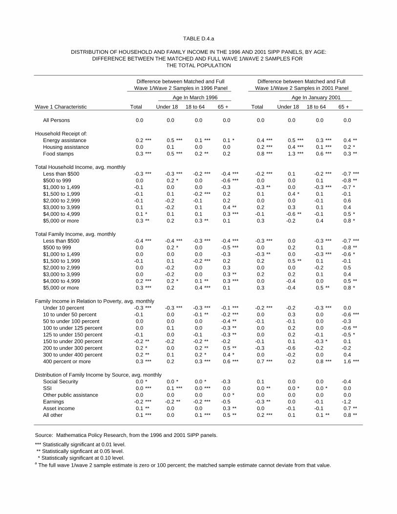
TABLE D.4.a

DISTRIBUTION OF HOUSEHOLD AND FAMILY INCOME IN THE 1996 AND 2001 SIPP PANELS, BY AGE:DIFFERENCE BETWEEN THE MATCHED AND FULL WAVE 1/WAVE 2 SAMPLES FOR

THE TOTAL POPULATION

Difference between Matched and Full Difference between Matched and Full Wave 1/Wave 2 Samples in 1996 Panel Wave 1/Wave 2 Samples in 2001 Panel

Age In March 1996 Age In January 2001

Wave 1 Characteristic Total Under 18 18 to 64 65 + Total Under 18 18 to 64 65 +

All Persons 0.0 0.0 0.0 0.0 0.0 0.0 0.0 0.0

Household Receipt of:Energy assistance 0.2 *** 0.5 *** 0.1 *** 0.1 * 0.4 *** 0.5 *** 0.3 *** 0.4 **Housing assistance 0.0 0.1 0.0 0.0 0.2 *** 0.4 *** 0.1 *** 0.2 *Food stamps 0.3 *** 0.5 *** 0.2 ** 0.2 0.8 *** 1.3 *** 0.6 *** 0.3 **

Total Household Income, avg. monthlyLess than $500 -0.3 *** -0.3 *** -0.2 *** -0.4 *** -0.2 *** 0.1 -0.2 *** -0.7 ***$500 to 999 0.0 0.2 * 0.0 -0.6 *** 0.0 0.0 0.1 -0.8 **$1,000 to 1,499 -0.1 0.0 0.0 -0.3 -0.3 ** 0.0 -0.3 *** -0.7 *$1,500 to 1,999 -0.1 0.1 -0.2 *** 0.2 0.1 0.4 * 0.1 -0.1 $2,000 to 2,999 -0.1 -0.2 -0.1 0.2 0.0 0.0 -0.1 0.6 $3,000 to 3,999 0.1 -0.2 0.1 0.4 ** 0.2 0.3 0.1 0.4 $4,000 to 4,999 0.1 * 0.1 0.1 0.3 *** -0.1 -0.6 ** -0.1 0.5 *$5,000 or more 0.3 ** 0.2 0.3 ** 0.1 0.3 -0.2 0.4 0.8 *

Total Family Income, avg. monthlyLess than $500 -0.4 *** -0.4 *** -0.3 *** -0.4 *** -0.3 *** 0.0 -0.3 *** -0.7 ***$500 to 999 0.0 0.2 * 0.0 -0.5 *** 0.0 0.2 0.1 -0.8 **$1,000 to 1,499 0.0 0.0 0.0 -0.3 -0.3 ** 0.0 -0.3 *** -0.6 *$1,500 to 1,999 -0.1 0.1 -0.2 *** 0.2 0.2 0.5 ** 0.1 -0.1 $2,000 to 2,999 0.0 -0.2 0.0 0.3 0.0 0.0 -0.2 0.5 $3,000 to 3,999 0.0 -0.2 0.0 0.3 ** 0.2 0.2 0.1 0.4 $4,000 to 4,999 0.2 *** 0.2 * 0.1 ** 0.3 *** 0.0 -0.4 0.0 0.5 **$5,000 or more 0.3 *** 0.2 0.4 *** 0.1 0.3 -0.4 0.5 ** 0.8 *

Family Income in Relation to Poverty, avg. monthlyUnder 10 percent -0.3 *** -0.3 *** -0.3 *** -0.1 *** -0.2 *** -0.2 -0.3 *** 0.0 10 to under 50 percent -0.1 0.0 -0.1 ** -0.2 *** 0.0 0.3 0.0 -0.6 ***50 to under 100 percent 0.0 0.0 0.0 -0.4 ** -0.1 -0.1 0.0 -0.3 100 to under 125 percent 0.0 0.1 0.0 -0.3 ** 0.0 0.2 0.0 -0.6 **125 to under 150 percent -0.1 0.0 -0.1 -0.3 ** 0.0 0.2 -0.1 -0.5 *150 to under 200 percent -0.2 ** -0.2 -0.2 ** -0.2 -0.1 0.1 -0.3 * 0.1 200 to under 300 percent 0.2 * 0.0 0.2 ** 0.5 ** -0.3 -0.6 -0.2 -0.2 300 to under 400 percent 0.2 ** 0.1 0.2 * 0.4 * 0.0 -0.2 0.0 0.4 400 percent or more 0.3 *** 0.2 0.3 *** 0.6 *** 0.7 *** 0.2 0.8 *** 1.6 ***

Distribution of Family Income by Source, avg. monthlySocial Security 0.0 * 0.0 * 0.0 * -0.3 0.1 0.0 0.0 -0.4 SSI 0.0 *** 0.1 *** 0.0 *** 0.0 0.0 ** 0.0 * 0.0 * 0.0 Other public assistance 0.0 0.0 0.0 0.0 * 0.0 0.0 0.0 0.0 Earnings -0.2 *** -0.2 ** -0.2 *** -0.5 -0.3 ** 0.0 -0.1 -1.2 Asset income 0.1 ** 0.0 0.0 0.3 ** 0.0 -0.1 -0.1 0.7 **All other 0.1 *** 0.0 0.1 *** 0.5 ** 0.2 *** 0.1 0.1 ** 0.8 **

Source: Mathematica Policy Research, from the 1996 and 2001 SIPP panels.

*** Statistically significant at 0.01 level. ** Statistically signficant at 0.05 level. * Statistically significant at 0.10 level.a The full wave 1/wave 2 sample estimate is zero or 100 percent; the matched sample estimate cannot deviate from that value.

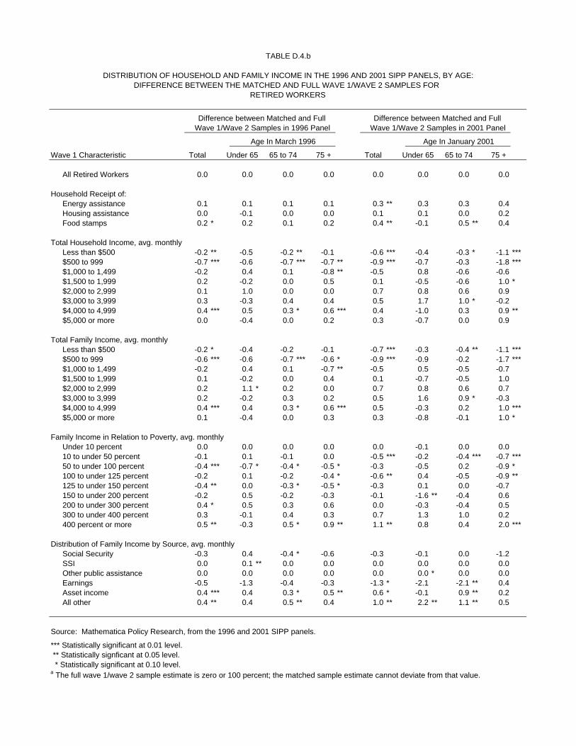
TABLE D.4.b

DISTRIBUTION OF HOUSEHOLD AND FAMILY INCOME IN THE 1996 AND 2001 SIPP PANELS, BY AGE:DIFFERENCE BETWEEN THE MATCHED AND FULL WAVE 1/WAVE 2 SAMPLES FOR

RETIRED WORKERS

Difference between Matched and Full Difference between Matched and Full Wave 1/Wave 2 Samples in 1996 Panel Wave 1/Wave 2 Samples in 2001 Panel

Age In March 1996 Age In January 2001

Wave 1 Characteristic Total Under 65 65 to 74 75 + Total Under 65 65 to 74 75 +

All Retired Workers 0.0 0.0 0.0 0.0 0.0 0.0 0.0 0.0

Household Receipt of:Energy assistance 0.1 0.1 0.1 0.1 0.3 ** 0.3 0.3 0.4 Housing assistance 0.0 -0.1 0.0 0.0 0.1 0.1 0.0 0.2 Food stamps 0.2 * 0.2 0.1 0.2 0.4 ** -0.1 0.5 ** 0.4

Total Household Income, avg. monthlyLess than $500 -0.2 ** -0.5 -0.2 ** -0.1 -0.6 *** -0.4 -0.3 * -1.1 ***$500 to 999 -0.7 *** -0.6 -0.7 *** -0.7 ** -0.9 *** -0.7 -0.3 -1.8 ***$1,000 to 1,499 -0.2 0.4 0.1 -0.8 ** -0.5 0.8 -0.6 -0.6 $1,500 to 1,999 0.2 -0.2 0.0 0.5 0.1 -0.5 -0.6 1.0 *$2,000 to 2,999 0.1 1.0 0.0 0.0 0.7 0.8 0.6 0.9 $3,000 to 3,999 0.3 -0.3 0.4 0.4 0.5 1.7 1.0 * -0.2 $4,000 to 4,999 0.4 *** 0.5 0.3 * 0.6 *** 0.4 -1.0 0.3 0.9 **$5,000 or more 0.0 -0.4 0.0 0.2 0.3 -0.7 0.0 0.9

Total Family Income, avg. monthlyLess than $500 -0.2 * -0.4 -0.2 -0.1 -0.7 *** -0.3 -0.4 ** -1.1 ***$500 to 999 -0.6 *** -0.6 -0.7 *** -0.6 * -0.9 *** -0.9 -0.2 -1.7 ***$1,000 to 1,499 -0.2 0.4 0.1 -0.7 ** -0.5 0.5 -0.5 -0.7 $1,500 to 1,999 0.1 -0.2 0.0 0.4 0.1 -0.7 -0.5 1.0 $2,000 to 2,999 0.2 1.1 * 0.2 0.0 0.7 0.8 0.6 0.7 $3,000 to 3,999 0.2 -0.2 0.3 0.2 0.5 1.6 0.9 * -0.3 $4,000 to 4,999 0.4 *** 0.4 0.3 * 0.6 *** 0.5 -0.3 0.2 1.0 ***$5,000 or more 0.1 -0.4 0.0 0.3 0.3 -0.8 -0.1 1.0 *

Family Income in Relation to Poverty, avg. monthlyUnder 10 percent 0.0 0.0 0.0 0.0 0.0 -0.1 0.0 0.0 10 to under 50 percent -0.1 0.1 -0.1 0.0 -0.5 *** -0.2 -0.4 *** -0.7 ***50 to under 100 percent -0.4 *** -0.7 * -0.4 * -0.5 * -0.3 -0.5 0.2 -0.9 *100 to under 125 percent -0.2 0.1 -0.2 -0.4 * -0.6 ** 0.4 -0.5 -0.9 **125 to under 150 percent -0.4 ** 0.0 -0.3 * -0.5 * -0.3 0.1 0.0 -0.7 150 to under 200 percent -0.2 0.5 -0.2 -0.3 -0.1 -1.6 ** -0.4 0.6 200 to under 300 percent 0.4 * 0.5 0.3 0.6 0.0 -0.3 -0.4 0.5 300 to under 400 percent 0.3 -0.1 0.4 0.3 0.7 1.3 1.0 0.2 400 percent or more 0.5 ** -0.3 0.5 * 0.9 ** 1.1 ** 0.8 0.4 2.0 ***

Distribution of Family Income by Source, avg. monthlySocial Security -0.3 0.4 -0.4 * -0.6 -0.3 -0.1 0.0 -1.2 SSI 0.0 0.1 ** 0.0 0.0 0.0 0.0 0.0 0.0 Other public assistance 0.0 0.0 0.0 0.0 0.0 0.0 * 0.0 0.0 Earnings -0.5 -1.3 -0.4 -0.3 -1.3 * -2.1 -2.1 ** 0.4 Asset income 0.4 *** 0.4 0.3 * 0.5 ** 0.6 * -0.1 0.9 ** 0.2 All other 0.4 ** 0.4 0.5 ** 0.4 1.0 ** 2.2 ** 1.1 ** 0.5

Source: Mathematica Policy Research, from the 1996 and 2001 SIPP panels.

*** Statistically significant at 0.01 level. ** Statistically signficant at 0.05 level. * Statistically significant at 0.10 level.a The full wave 1/wave 2 sample estimate is zero or 100 percent; the matched sample estimate cannot deviate from that value.

TABLE D.4.c

DISTRIBUTION OF HOUSEHOLD AND FAMILY INCOME IN THE 1996 AND 2001 SIPP PANELS, BY AGE:DIFFERENCE BETWEEN THE MATCHED AND FULL WAVE 1/WAVE 2 SAMPLES FOR

DISABLED WORKERS

Difference between Matched and Full Difference between Matched and Full Wave 1/Wave 2 Samples in 1996 Panel Wave 1/Wave 2 Samples in 2001 Panel

Age In March 1996 Age In January 2001

Wave 1 Characteristic Total Under 50 50 to 64 65 + Total Under 50 50 to 64 65 +

All Disabled Workers 0.0 0.0 0.0 0.0 0.0 0.0 0.0 0.0

Household Receipt of:Energy assistance 0.2 0.0 0.2 0.3 0.6 0.0 1.2 0.5 Housing assistance 0.0 0.2 0.0 -0.4 0.6 -0.1 0.9 1.0 Food stamps 0.5 0.3 1.0 * -0.6 1.5 * -0.3 2.7 *** 1.5

Total Household Income, avg. monthlyLess than $500 0.1 0.1 0.1 0.3 -0.6 ** -0.8 * -0.9 ** 0.2 $500 to 999 -0.2 0.3 0.0 -1.3 0.5 -1.4 1.5 1.9 $1,000 to 1,499 -0.3 -0.8 -0.3 0.2 -1.0 -0.2 -1.4 -1.4 $1,500 to 1,999 -0.2 -0.4 -0.5 0.5 0.8 2.6 ** 0.8 -2.1 $2,000 to 2,999 0.2 -0.5 1.0 0.0 0.4 1.1 -1.6 2.7 *$3,000 to 3,999 0.0 0.5 -0.4 0.0 0.0 -0.7 1.0 -1.0 $4,000 to 4,999 0.3 0.5 *** 0.4 0.0 0.9 0.2 1.5 1.1 $5,000 or more 0.1 0.2 -0.3 0.2 -1.0 -1.0 -0.9 -1.4

Total Family Income, avg. monthlyLess than $500 0.2 0.0 0.1 0.4 -0.6 ** -0.6 -1.1 ** 0.2 $500 to 999 -0.1 0.9 -0.5 -1.1 -0.1 -1.7 0.0 2.1 $1,000 to 1,499 -0.5 -0.7 -0.4 -0.3 -0.6 -0.3 -0.8 -1.0 $1,500 to 1,999 0.1 -0.4 0.2 0.8 0.7 2.1 ** 1.1 -2.2 $2,000 to 2,999 0.0 -0.6 0.6 -0.5 0.8 2.0 * -1.1 2.5 $3,000 to 3,999 0.2 0.5 -0.2 0.3 0.0 -0.6 1.1 -0.8 $4,000 to 4,999 0.3 0.4 *** 0.5 0.0 1.0 * 0.6 1.6 * 0.7 $5,000 or more -0.1 -0.1 -0.3 0.3 -1.2 * -1.6 -0.7 -1.6

Family Income in Relation to Poverty, avg. monthlyUnder 10 percent 0.0 0.0 0.0 a 0.0 a 0.0 -0.2 0.1 0.2 10 to under 50 percent 0.2 0.3 ** 0.2 -0.1 -0.2 0.1 -0.5 0.0 50 to under 100 percent -0.2 0.0 -0.4 -0.6 0.6 -0.9 0.0 3.5 **100 to under 125 percent 0.1 0.7 ** -0.1 -0.5 -0.3 0.4 0.3 -2.5 125 to under 150 percent -0.4 0.3 -0.9 -0.8 -0.2 0.2 -0.1 -1.1 150 to under 200 percent 0.1 -0.8 0.5 0.9 0.4 0.8 0.3 0.0 200 to under 300 percent 0.2 -0.7 0.7 0.7 -0.8 0.2 -2.2 0.7 300 to under 400 percent 0.0 0.3 -0.2 0.0 0.2 -0.7 1.2 -0.3 400 percent or more 0.0 -0.1 0.2 0.3 0.2 0.2 0.9 -0.4

Distribution of Family Income by Source, avg. monthlySocial Security -0.5 -0.8 -0.2 -0.8 0.7 1.8 -0.1 0.9 SSI 0.1 0.1 0.0 0.2 0.0 -0.2 0.0 0.4 Other public assistance 0.0 -0.1 -0.1 0.1 0.2 ** 0.3 0.2 * 0.3 **Earnings 0.3 0.9 -0.3 0.2 -0.1 -1.3 1.2 -1.7 Asset income 0.2 * 0.2 0.2 0.4 0.4 0.4 0.2 0.7 All other 0.0 -0.4 0.4 0.0 -1.3 -0.9 -1.7 -0.7

Source: Mathematica Policy Research, from the 1996 and 2001 SIPP panels.

*** Statistically significant at 0.01 level. ** Statistically signficant at 0.05 level. * Statistically significant at 0.10 level.a The full wave 1/wave 2 sample estimate is zero or 100 percent; the matched sample estimate cannot deviate from that value.

TABLE D.4.d

DISTRIBUTION OF HOUSEHOLD AND FAMILY INCOME IN THE 1996 AND 2001 SIPP PANELS, BY AGE:DIFFERENCE BETWEEN THE MATCHED AND FULL WAVE 1/WAVE 2 SAMPLES FOR

ALL OTHER SOCIAL SECURITY BENEFICIARIES

Difference between Matched and Full Difference between Matched and Full Wave 1/Wave 2 Samples in 1996 Panel Wave 1/Wave 2 Samples in 2001 Panel

Age In March 1996 Age In January 2001

Wave 1 Characteristic Total Under 18 18 to 64 65 + Total Under 18 18 to 64 65 +

All Other Beneficiaries 0.0 0.0 0.0 0.0 0.0 0.0 0.0 0.0

Household Receipt of:Energy assistance 0.1 0.1 -0.1 0.1 1.3 *** 2.8 *** 1.9 ** 0.3 Housing assistance 0.0 0.2 -0.5 0.1 0.2 0.2 -0.1 0.2 Food stamps 0.6 ** 1.0 0.3 0.3 * 1.1 ** 1.0 2.1 ** 0.6 *

Total Household Income, avg. monthlyLess than $500 -0.6 *** -0.2 -0.4 -0.8 *** -0.9 ** 0.0 -0.6 -1.3 **$500 to 999 -0.8 ** 0.7 -1.4 * -1.1 ** 0.5 -0.9 2.8 ** 0.9 $1,000 to 1,499 0.3 0.7 1.9 *** -0.3 -1.6 ** 0.3 -0.1 -2.6 **$1,500 to 1,999 0.2 -0.1 0.1 0.4 -0.3 0.7 0.1 -0.7 $2,000 to 2,999 0.6 -0.4 -0.2 1.1 *** 0.5 2.0 -1.4 0.2 $3,000 to 3,999 0.7 *** 0.8 0.5 0.6 ** 0.8 -0.6 3.6 ** 0.4 $4,000 to 4,999 0.0 -0.1 0.3 -0.1 0.0 0.3 -3.3 *** 0.7 $5,000 or more -0.2 -1.4 * -0.8 0.3 1.1 -1.7 -0.9 2.4 ***

Total Family Income, avg. monthlyLess than $500 -0.8 *** -0.6 -0.6 -0.9 *** -1.0 *** -0.6 -0.4 -1.4 **$500 to 999 -0.8 ** 0.8 -1.5 * -1.1 ** 0.7 -0.6 2.5 * 1.2 $1,000 to 1,499 0.3 0.9 1.8 *** -0.2 -1.8 ** 0.5 -0.4 -2.9 ***$1,500 to 1,999 0.1 -0.2 -0.3 0.4 -0.3 0.3 -0.4 -0.4 $2,000 to 2,999 0.7 ** -0.3 0.5 1.1 *** 0.8 2.5 -0.4 0.3 $3,000 to 3,999 0.6 *** 0.8 0.3 0.5 ** 0.6 -0.7 3.6 ** 0.2 $4,000 to 4,999 0.0 0.1 0.4 -0.1 0.0 0.3 -3.3 *** 0.6 $5,000 or more -0.2 -1.4 * -0.6 0.4 1.0 -1.6 -1.3 2.4 ***

Family Income in Relation to Poverty, avg. monthlyUnder 10 percent 0.0 -0.1 0.0 a 0.0 -0.2 -0.8 0.0 a -0.1 10 to under 50 percent -0.2 0.3 -0.1 -0.4 ** -0.6 * -0.4 -0.2 -0.8 **50 to under 100 percent -0.4 0.9 -1.3 * -0.8 * 1.0 1.4 2.0 0.6 100 to under 125 percent -0.1 0.1 0.0 -0.2 0.5 0.6 1.7 * 0.1 125 to under 150 percent -0.3 0.3 -0.2 -0.5 -0.7 1.2 -0.4 -1.6 **150 to under 200 percent -0.1 -1.2 1.3 ** 0.0 -0.8 -1.5 0.6 -0.9 200 to under 300 percent 0.8 ** 0.6 1.0 0.8 ** -0.2 1.4 -1.4 -0.5 300 to under 400 percent 0.3 -0.5 -0.2 0.8 *** -0.6 -1.5 0.6 -0.7 400 percent or more 0.0 -0.5 -0.5 0.3 1.7 * -0.3 -3.0 3.8 ***

Distribution of Family Income by Source, avg. monthlySocial Security 0.1 1.2 * 0.4 -0.5 -1.3 ** -0.6 0.4 -2.0 **SSI 0.1 ** 0.1 0.3 *** 0.0 0.0 -0.3 0.4 0.0 Other public assistance 0.0 0.1 -0.1 * 0.0 ** 0.0 0.0 -0.4 0.0 Earnings -0.8 -1.9 ** -1.8 * 0.3 1.7 * 0.5 -1.7 2.9 **Asset income 0.2 0.1 0.5 ** 0.0 0.3 0.5 1.5 * 0.0 All other 0.4 * 0.5 0.7 0.2 -0.6 -0.2 -0.1 -0.9

Source: Mathematica Policy Research, from the 1996 and 2001 SIPP panels.

*** Statistically significant at 0.01 level. ** Statistically signficant at 0.05 level. * Statistically significant at 0.10 level.a The full wave 1/wave 2 sample estimate is zero or 100 percent; the matched sample estimate cannot deviate from that value.

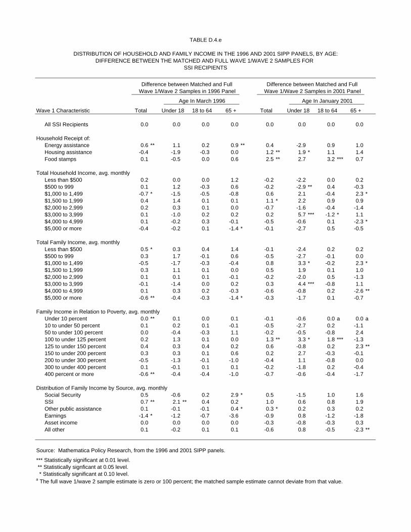
TABLE D.4.e

DISTRIBUTION OF HOUSEHOLD AND FAMILY INCOME IN THE 1996 AND 2001 SIPP PANELS, BY AGE:DIFFERENCE BETWEEN THE MATCHED AND FULL WAVE 1/WAVE 2 SAMPLES FOR

SSI RECIPIENTS

Difference between Matched and Full Difference between Matched and Full Wave 1/Wave 2 Samples in 1996 Panel Wave 1/Wave 2 Samples in 2001 Panel

Age In March 1996 Age In January 2001

Wave 1 Characteristic Total Under 18 18 to 64 65 + Total Under 18 18 to 64 65 +

All SSI Recipients 0.0 0.0 0.0 0.0 0.0 0.0 0.0 0.0

Household Receipt of:Energy assistance 0.6 ** 1.1 0.2 0.9 ** 0.4 -2.9 0.9 1.0 Housing assistance -0.4 -1.9 -0.3 0.0 1.2 ** 1.9 * 1.1 1.4 Food stamps 0.1 -0.5 0.0 0.6 2.5 ** 2.7 3.2 *** 0.7

Total Household Income, avg. monthlyLess than $500 0.2 0.0 0.0 1.2 -0.2 -2.2 0.0 0.2 $500 to 999 0.1 1.2 -0.3 0.6 -0.2 -2.9 ** 0.4 -0.3 $1,000 to 1,499 -0.7 * -1.5 -0.5 -0.8 0.6 2.1 -0.4 2.3 *$1,500 to 1,999 0.4 1.4 0.1 0.1 1.1 * 2.2 0.9 0.9 $2,000 to 2,999 0.2 0.3 0.1 0.0 -0.7 -1.6 -0.4 -1.4 $3,000 to 3,999 0.1 -1.0 0.2 0.2 0.2 5.7 *** -1.2 * 1.1 $4,000 to 4,999 0.1 -0.2 0.3 -0.1 -0.5 -0.6 0.1 -2.3 *$5,000 or more -0.4 -0.2 0.1 -1.4 * -0.1 -2.7 0.5 -0.5

Total Family Income, avg. monthlyLess than $500 0.5 * 0.3 0.4 1.4 -0.1 -2.4 0.2 0.2 $500 to 999 0.3 1.7 -0.1 0.6 -0.5 -2.7 -0.1 0.0 $1,000 to 1,499 -0.5 -1.7 -0.3 -0.4 0.8 3.3 * -0.2 2.3 *$1,500 to 1,999 0.3 1.1 0.1 0.0 0.5 1.9 0.1 1.0 $2,000 to 2,999 0.1 0.1 0.1 -0.1 -0.2 -2.0 0.5 -1.3 $3,000 to 3,999 -0.1 -1.4 0.0 0.2 0.3 4.4 *** -0.8 1.1 $4,000 to 4,999 0.1 0.3 0.2 -0.3 -0.6 -0.8 0.2 -2.6 **$5,000 or more -0.6 ** -0.4 -0.3 -1.4 * -0.3 -1.7 0.1 -0.7

Family Income in Relation to Poverty, avg. monthlyUnder 10 percent 0.0 ** 0.1 0.0 0.1 -0.1 -0.6 0.0 a 0.0 a10 to under 50 percent 0.1 0.2 0.1 -0.1 -0.5 -2.7 0.2 -1.1 50 to under 100 percent 0.0 -0.4 -0.3 1.1 -0.2 -0.5 -0.8 2.4 100 to under 125 percent 0.2 1.3 0.1 0.0 1.3 ** 3.3 * 1.8 *** -1.3 125 to under 150 percent 0.4 0.3 0.4 0.2 0.6 -0.8 0.2 2.3 **150 to under 200 percent 0.3 0.3 0.1 0.6 0.2 2.7 -0.3 -0.1 200 to under 300 percent -0.5 -1.3 -0.1 -1.0 -0.4 1.1 -0.8 0.0 300 to under 400 percent 0.1 -0.1 0.1 0.1 -0.2 -1.8 0.2 -0.4 400 percent or more -0.6 ** -0.4 -0.4 -1.0 -0.7 -0.6 -0.4 -1.7

Distribution of Family Income by Source, avg. monthlySocial Security 0.5 -0.6 0.2 2.9 * 0.5 -1.5 1.0 1.6 SSI 0.7 ** 2.1 ** 0.4 0.2 1.0 0.6 0.8 1.9 Other public assistance 0.1 -0.1 -0.1 0.4 * 0.3 * 0.2 0.3 0.2 Earnings -1.4 * -1.2 -0.7 -3.6 -0.9 0.8 -1.2 -1.8 Asset income 0.0 0.0 0.0 0.0 -0.3 -0.8 -0.3 0.3 All other 0.1 -0.2 0.1 0.1 -0.6 0.8 -0.5 -2.3 **

Source: Mathematica Policy Research, from the 1996 and 2001 SIPP panels.

*** Statistically significant at 0.01 level. ** Statistically signficant at 0.05 level. * Statistically significant at 0.10 level.a The full wave 1/wave 2 sample estimate is zero or 100 percent; the matched sample estimate cannot deviate from that value.

E-1

APPENDIX E

COMPARISON OF DIFFERENCES BETWEEN MATCHED AND ENTIRE FULL PANEL SAMPLES: 1996 AND 2001 SIPP PANELS

TABLE E.1.a

DISTRIBUTION OF PERSONAL CHARACTERISTICS IN THE 1996 AND 2001 SIPP PANELS, BY AGE:DIFFERENCE BETWEEN THE MATCHED FULL PANEL AND ENTIRE FULL PANEL SAMPLES FOR

THE TOTAL POPULATION

Difference between Matched Full Panel Difference between Matched Full Paneland Full Panel Samples in 1996 Panel and Full Panel Samples in 2001 Panel

Age In March 1996 Age In January 2001

Wave 1 Characteristic Total Under 18 18 to 64 65 + Total Under 18 18 to 64 65 +

All Persons 0.0 0.0 0.0 0.0 0.0 0.0 0.0 0.0

SexMale 0.0 0.0 0.0 0.0 0.0 -0.1 0.0 0.0 Female 0.0 0.0 0.0 0.0 0.0 0.1 0.0 0.0

RaceWhite 0.4 *** 0.2 * 0.5 *** 0.3 0.4 *** 0.1 0.6 *** -0.1 Black 0.0 0.1 0.0 -0.1 0.0 0.2 ** -0.1 ** 0.0 American Indian, Alaska Native 0.1 *** 0.1 ** 0.1 ** 0.1 * 0.2 ** 0.4 *** 0.1 0.0 Asian, Pacific Islander -0.4 *** -0.4 *** -0.5 *** -0.2 * -0.6 *** -0.7 *** -0.6 *** 0.0

EthnicityHispanic 0.0 0.1 -0.1 0.1 0.0 0.2 -0.1 * 0.1 Non-Hispanic 0.0 -0.1 0.1 -0.1 0.0 -0.2 0.1 * -0.1

Marital StatusMarried -0.1 ** 0.0 -0.1 -0.3 -0.2 *** 0.0 -0.4 *** 1.0 *Widowed 0.0 0.0 0.0 0.0 -0.2 *** 0.0 a -0.1 -1.2 ***Divorced or separated 0.2 *** 0.0 0.3 *** 0.2 0.0 0.0 0.1 -0.1 Never married -0.1 0.0 * -0.2 * 0.1 0.3 *** 0.0 0.4 ** 0.4

Years of education0 to 8 -0.3 *** 0.0 -0.3 *** -0.4 * -0.3 *** -0.1 -0.4 *** -0.2 9 to 11 0.1 * 0.1 0.1 0.2 0.1 0.3 0.1 -0.4 12 -0.3 *** 0.0 -0.3 ** -0.6 ** -0.5 *** 0.0 -0.7 ** -0.6 13 to 15 0.4 *** 0.0 0.6 *** 0.5 *** 0.6 *** 0.0 1.0 *** 0.7 *16 or more 0.0 0.0 a 0.0 0.2 0.1 0.0 a 0.0 0.5 Unknown (used for children) 0.0 0.0 0.0 a 0.0 a 0.0 -0.2 0.0 a 0.0 a

Living ArrangementLives alone 0.0 0.0 a 0.0 0.1 0.0 0.0 0.3 *** -1.6 ***Lives with relatives 0.1 ** 0.1 * 0.2 * -0.2 0.1 0.0 -0.1 1.4 ***Lives with only non-relatives -0.1 ** -0.1 * -0.2 ** 0.0 -0.1 0.0 -0.2 0.2

Relationship to HouseholderHouseholder 0.2 *** 0.0 0.4 *** 0.0 0.4 *** 0.0 0.9 *** -1.2 ***Spouse -0.2 *** 0.0 * -0.2 *** -0.3 * -0.3 *** 0.0 -0.7 *** 0.8 **Child 0.4 *** 0.6 *** 0.3 *** 0.0 * 0.3 ** 0.4 0.2 0.0 Grandchild -0.1 -0.1 0.0 0.0 a -0.1 -0.3 0.0 0.0 aParent 0.0 * 0.0 a -0.1 *** 0.0 0.0 0.0 a 0.0 0.2 Sibling -0.1 *** 0.0 -0.1 ** 0.0 0.0 0.0 -0.1 0.2 *Other relative -0.1 *** -0.2 ** -0.2 *** 0.2 * -0.2 *** -0.1 -0.3 *** -0.2 Nonrelative -0.1 *** -0.2 *** -0.1 ** 0.1 -0.1 0.0 -0.2 0.1

Parents PresentBoth mother and father 0.2 ** 0.2 0.2 ** 0.0 -0.2 -1.4 *** 0.1 0.0 aMother only 0.1 0.1 0.1 0.0 0.3 ** 1.1 *** 0.0 0.0 Father only -0.1 * -0.2 ** 0.0 0.0 0.1 ** 0.3 * 0.1 0.0 Neither -0.2 *** -0.2 ** -0.2 ** 0.0 -0.2 0.0 -0.2 0.0

Source: Mathematica Policy Research, from the 1996 and 2001 SIPP panels.

*** Statistically significant at 0.01 level. ** Statistically signficant at 0.05 level. * Statistically significant at 0.10 level.a The full panel sample estimate is zero or 100 percent; the matched full panel sample estimate cannot deviate from that value.

TABLE E.1.b

DISTRIBUTION OF PERSONAL CHARACTERISTICS IN THE 1996 AND 2001 SIPP PANELS, BY AGE:DIFFERENCE BETWEEN THE MATCHED FULL PANEL AND ENTIRE FULL PANEL SAMPLES FOR

RETIRED WORKERS

Difference between Matched Full Panel Difference between Matched Full Paneland Full Panel Samples in 1996 Panel and Full Panel Samples in 2001 Panel

Age In March 1996 Age In January 2001

Wave 1 Characteristic Total Under 65 65 to 74 75 + Total Under 65 65 to 74 75 +

All Retired Workers 0.0 0.0 0.0 0.0 0.0 0.0 0.0 0.0

SexMale -0.1 -0.5 -0.2 0.2 -0.4 * -0.3 -0.8 ** 0.0 Female 0.1 0.5 0.2 -0.2 0.4 * 0.3 0.8 ** 0.0

RaceWhite 0.2 * 1.2 * 0.1 0.2 0.3 3.5 *** -0.6 0.5 Black -0.3 * -0.8 -0.1 -0.3 -0.2 -2.7 *** 0.7 ** -0.5 American Indian, Alaska Native 0.1 0.1 * 0.0 0.1 0.1 0.1 0.1 0.0 Asian, Pacific Islander 0.0 -0.5 0.0 0.0 -0.2 -0.9 * -0.1 0.0

EthnicityHispanic 0.0 -0.3 0.2 -0.1 0.0 0.7 -0.5 0.4 Non-Hispanic 0.0 0.3 -0.2 0.1 0.0 -0.7 0.5 -0.4

Marital StatusMarried -0.4 0.3 0.2 -1.3 ** 0.9 * 0.8 1.1 * 0.7 Widowed 0.1 0.0 -0.2 0.5 -0.9 ** 0.0 -1.1 ** -0.9 Divorced or separated 0.1 -0.3 -0.1 0.4 * -0.3 -0.8 -0.3 -0.1 Never married 0.2 ** 0.0 0.1 0.4 ** 0.2 0.0 0.2 0.3

Years of education0 to 8 -0.5 ** 0.1 -0.4 -0.7 -0.3 -0.9 0.7 * -1.3 **9 to 11 0.2 -0.4 0.1 0.4 -0.4 -1.8 * -0.5 0.1 12 -0.5 * -0.4 -0.5 -0.5 -0.7 -0.7 -1.3 ** 0.0 13 to 15 0.6 *** 0.4 0.4 0.9 ** 1.1 ** 2.8 ** 0.5 1.3 **16 or more 0.2 0.3 0.4 0.0 0.3 0.5 0.6 -0.1 Unknown (used for children) 0.0 a 0.0 a 0.0 a 0.0 a 0.0 a 0.0 a 0.0 a 0.0 a

Living ArrangementLives alone 0.1 -0.5 -0.1 0.3 -1.4 *** 0.4 -0.8 -2.6 ***Lives with relatives -0.2 0.2 -0.1 -0.5 1.6 *** 0.8 1.0 * 2.4 ***Lives with only non-relatives 0.2 0.3 0.1 0.1 -0.1 -1.2 * -0.2 0.2

Relationship to HouseholderHouseholder -0.2 0.5 -0.2 -0.3 -1.0 ** 3.9 *** -1.6 *** -1.5 **Spouse -0.4 ** -0.4 -0.1 -0.7 ** 0.7 * -1.8 1.6 *** 0.3 Child 0.0 ** 0.2 * 0.0 0.0 a 0.0 0.2 0.0 0.0 aGrandchild 0.0 a 0.0 a 0.0 a 0.0 a 0.0 0.1 0.0 a 0.0 aParent 0.1 -0.1 0.1 0.3 0.3 * -0.2 0.1 0.8 *Sibling 0.0 0.1 -0.1 0.1 0.2 -0.1 0.3 ** 0.1 Other relative 0.2 ** -0.6 0.1 0.5 *** -0.1 -0.5 -0.3 0.2 Nonrelative 0.2 ** 0.3 ** 0.1 0.2 -0.1 -1.6 ** -0.1 0.1

Parents PresentBoth mother and father 0.0 0.0 a 0.0 0.0 a 0.0 0.2 0.0 a 0.0 aMother only 0.0 0.2 * 0.0 0.0 -0.1 -0.3 -0.1 0.0 Father only 0.0 0.0 0.0 0.0 a 0.0 0.1 0.0 0.0 aNeither 0.0 -0.2 ** 0.0 0.0 0.1 -0.1 0.1 0.0

Source: Mathematica Policy Research, from the 1996 and 2001 SIPP panels.

*** Statistically significant at 0.01 level. ** Statistically signficant at 0.05 level. * Statistically significant at 0.10 level.a The full panel sample estimate is zero or 100 percent; the matched full panel sample estimate cannot deviate from that value.

TABLE E.1.c

DISTRIBUTION OF PERSONAL CHARACTERISTICS IN THE 1996 AND 2001 SIPP PANELS, BY AGE:DIFFERENCE BETWEEN THE MATCHED FULL PANEL AND ENTIRE FULL PANEL SAMPLES FOR

DISABLED WORKERS

Difference between Matched Full Panel Difference between Matched Full Paneland Full Panel Samples in 1996 Panel and Full Panel Samples in 2001 Panel

Age In March 1996 Age In January 2001

Wave 1 Characteristic Total Under 50 50 to 64 65 + Total Under 50 50 to 64 65 +

All Disabled Workers 0.0 0.0 0.0 0.0 0.0 0.0 0.0 0.0

SexMale 0.0 1.1 -1.0 -0.6 -1.0 -1.0 -2.7 * 1.5 Female 0.0 -1.1 1.0 0.6 1.0 1.0 2.7 * -1.5

RaceWhite -1.0 -0.9 -1.4 * -0.6 -1.3 -1.6 -0.9 -1.1 Black 0.7 0.5 1.4 ** -0.1 1.0 1.7 0.8 -0.2 American Indian, Alaska Native 0.2 *** 0.1 0.1 *** 0.3 * 0.4 * 0.5 * 0.3 0.3 Asian, Pacific Islander 0.1 0.2 * -0.2 0.4 * 0.0 -0.6 -0.2 1.0 *

EthnicityHispanic 0.3 0.5 0.7 ** -0.6 1.6 ** 2.2 * 0.8 2.2 Non-Hispanic -0.3 -0.5 -0.7 ** 0.6 -1.6 ** -2.2 * -0.8 -2.2

Marital StatusMarried -0.3 0.3 -0.5 0.3 1.1 1.7 2.1 0.1 Widowed -0.5 -0.1 -0.1 -0.6 -1.1 -1.0 0.8 -3.6 Divorced or separated 0.0 -0.5 0.8 -0.4 0.0 0.8 -1.2 1.6 Never married 0.8 0.4 -0.2 0.7 0.0 -1.5 -1.7 * 1.9 **

Years of education0 to 8 -0.8 -1.9 * 1.6 ** -2.0 0.0 1.4 -1.8 1.5 9 to 11 0.2 1.2 * 0.6 -1.6 -1.8 ** -3.5 ** 0.0 -1.9 12 0.2 0.6 -1.9 ** 1.9 ** 0.2 -0.4 0.4 0.1 13 to 15 0.7 ** 0.5 0.3 1.6 *** 0.7 0.6 1.5 -0.9 16 or more -0.3 -0.4 -0.5 0.1 0.9 * 1.9 *** -0.1 1.3 Unknown (used for children) 0.0 a 0.0 a 0.0 a 0.0 a 0.0 a 0.0 a 0.0 a 0.0 a

Living ArrangementLives alone -0.3 -0.9 0.3 0.1 -0.3 1.3 -0.9 -0.8 Lives with relatives 0.2 0.3 0.1 0.0 0.9 -0.4 2.5 -0.1 Lives with only non-relatives 0.2 0.7 -0.3 -0.1 -0.6 -0.9 -1.6 * 1.0

Relationship to HouseholderHouseholder -0.7 -0.5 0.4 -1.7 0.9 -0.1 2.0 1.7 Spouse -0.4 -0.3 -0.9 0.6 0.4 1.3 1.5 -2.2 Child 0.0 -0.7 -0.3 0.1 -0.4 -0.5 -1.5 * 0.0 aGrandchild -0.1 -0.3 0.0 a 0.0 a 0.1 0.3 0.0 a 0.0 aParent 0.1 0.0 a 0.3 0.3 0.0 0.2 0.6 -1.0 Sibling 0.2 0.7 0.2 -0.4 -0.3 -0.3 -1.1 * 1.0 Other relative 0.4 * 0.5 *** 0.2 0.6 -0.1 0.0 -0.3 0.0 Nonrelative 0.5 0.6 0.1 0.6 -0.6 -0.9 -1.3 * 0.6

Parents PresentBoth mother and father 0.2 0.1 0.0 0.1 0.0 -0.4 -0.2 0.0 aMother only -0.4 -1.0 -0.3 -0.2 -0.3 -0.9 -0.4 0.0 aFather only 0.1 0.5 *** -0.2 0.0 a 0.2 0.5 0.0 0.0 aNeither 0.0 0.5 0.5 0.1 0.1 0.8 0.6 0.0 a

Source: Mathematica Policy Research, from the 1996 and 2001 SIPP panels.

*** Statistically significant at 0.01 level. ** Statistically signficant at 0.05 level. * Statistically significant at 0.10 level.a The full panel sample estimate is zero or 100 percent; the matched full panel sample estimate cannot deviate from that value.

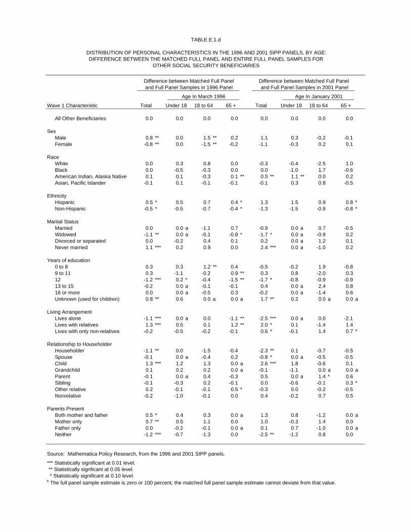
TABLE E.1.d

DISTRIBUTION OF PERSONAL CHARACTERISTICS IN THE 1996 AND 2001 SIPP PANELS, BY AGE:DIFFERENCE BETWEEN THE MATCHED FULL PANEL AND ENTIRE FULL PANEL SAMPLES FOR

OTHER SOCIAL SECURITY BENEFICIARIES

Difference between Matched Full Panel Difference between Matched Full Paneland Full Panel Samples in 1996 Panel and Full Panel Samples in 2001 Panel

Age In March 1996 Age In January 2001

Wave 1 Characteristic Total Under 18 18 to 64 65 + Total Under 18 18 to 64 65 +

All Other Beneficiaries 0.0 0.0 0.0 0.0 0.0 0.0 0.0 0.0

SexMale 0.8 ** 0.0 1.5 ** 0.2 1.1 0.3 -0.2 -0.1 Female -0.8 ** 0.0 -1.5 ** -0.2 -1.1 -0.3 0.2 0.1

RaceWhite 0.0 0.3 0.8 0.0 -0.3 -0.4 -2.5 1.0 Black 0.0 -0.5 -0.3 0.0 0.0 -1.0 1.7 -0.6 American Indian, Alaska Native 0.1 0.1 -0.3 0.1 ** 0.5 ** 1.1 ** 0.0 0.2 Asian, Pacific Islander -0.1 0.1 -0.1 -0.1 -0.1 0.3 0.8 -0.5

EthnicityHispanic 0.5 * 0.5 0.7 0.4 * 1.3 1.5 0.9 0.8 *Non-Hispanic -0.5 * -0.5 -0.7 -0.4 * -1.3 -1.5 -0.9 -0.8 *

Marital StatusMarried 0.0 0.0 a -1.1 0.7 -0.9 0.0 a 0.7 -0.5 Widowed -1.1 ** 0.0 a -0.1 -0.8 * -1.7 * 0.0 a -0.9 0.2 Divorced or separated 0.0 -0.2 0.4 0.1 0.2 0.0 a 1.2 0.1 Never married 1.1 *** 0.2 0.9 0.0 2.4 *** 0.0 a -1.0 0.2

Years of education0 to 8 0.3 0.3 1.2 ** 0.4 -0.5 -0.2 1.9 -0.8 9 to 11 0.3 -1.1 -0.2 0.9 ** 0.3 0.8 -2.0 0.3 12 -1.2 *** 0.2 * -0.4 -1.5 ** -1.7 * -0.8 -0.9 -0.9 13 to 15 -0.2 0.0 a -0.1 -0.1 0.4 0.0 a 2.4 0.8 16 or more 0.0 0.0 a -0.5 0.3 -0.2 0.0 a -1.4 0.6 Unknown (used for children) 0.8 ** 0.6 0.0 a 0.0 a 1.7 ** 0.2 0.0 a 0.0 a

Living ArrangementLives alone -1.1 *** 0.0 a 0.0 -1.1 ** -2.5 *** 0.0 a 0.0 -2.1 Lives with relatives 1.3 *** 0.5 0.1 1.2 ** 2.0 * 0.1 -1.4 1.4 Lives with only non-relatives -0.2 -0.5 -0.2 -0.1 0.6 * -0.1 1.4 0.7 *

Relationship to HouseholderHouseholder -1.1 ** 0.0 -1.5 -0.4 -2.3 ** 0.1 -0.7 -0.5 Spouse -0.1 0.0 a -0.4 0.2 -0.8 * 0.0 a -0.5 -0.5 Child 1.3 *** 1.2 1.3 0.0 a 2.6 *** 1.8 -0.6 0.1 Grandchild 0.1 0.2 0.2 0.0 a -0.1 -1.1 0.0 a 0.0 aParent -0.1 0.0 a 0.4 -0.3 0.5 0.0 a 1.4 * 0.6 Sibling -0.1 -0.3 0.2 -0.1 0.0 -0.6 -0.1 0.3 *Other relative 0.2 -0.1 -0.1 0.5 * -0.3 0.0 -0.2 -0.5 Nonrelative -0.2 -1.0 -0.1 0.0 0.4 -0.2 0.7 0.5

Parents PresentBoth mother and father 0.5 * 0.4 0.3 0.0 a 1.3 0.8 -1.2 0.0 aMother only 0.7 ** 0.5 1.1 0.0 1.0 -0.3 1.4 0.0 Father only 0.0 -0.2 -0.1 0.0 a 0.1 0.7 -1.0 0.0 aNeither -1.2 *** -0.7 -1.3 0.0 -2.5 ** -1.2 0.8 0.0

Source: Mathematica Policy Research, from the 1996 and 2001 SIPP panels.

*** Statistically significant at 0.01 level. ** Statistically signficant at 0.05 level. * Statistically significant at 0.10 level.a The full panel sample estimate is zero or 100 percent; the matched full panel sample estimate cannot deviate from that value.

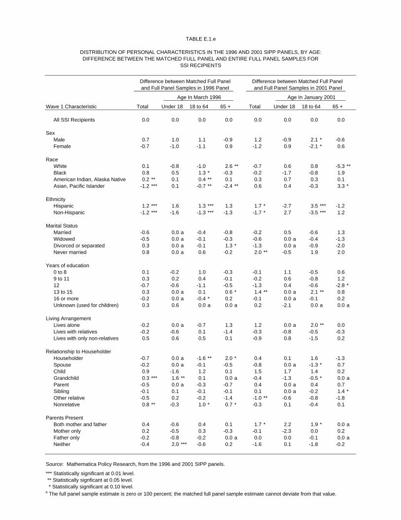
TABLE E.1.e

DISTRIBUTION OF PERSONAL CHARACTERISTICS IN THE 1996 AND 2001 SIPP PANELS, BY AGE:DIFFERENCE BETWEEN THE MATCHED FULL PANEL AND ENTIRE FULL PANEL SAMPLES FOR

SSI RECIPIENTS

Difference between Matched Full Panel Difference between Matched Full Paneland Full Panel Samples in 1996 Panel and Full Panel Samples in 2001 Panel

Age In March 1996 Age In January 2001

Wave 1 Characteristic Total Under 18 18 to 64 65 + Total Under 18 18 to 64 65 +

All SSI Recipients 0.0 0.0 0.0 0.0 0.0 0.0 0.0 0.0

SexMale 0.7 1.0 1.1 -0.9 1.2 -0.9 2.1 * -0.6 Female -0.7 -1.0 -1.1 0.9 -1.2 0.9 -2.1 * 0.6

RaceWhite 0.1 -0.8 -1.0 2.6 ** -0.7 0.6 0.8 -5.3 **Black 0.8 0.5 1.3 * -0.3 -0.2 -1.7 -0.8 1.9 American Indian, Alaska Native 0.2 ** 0.1 0.4 ** 0.1 0.3 0.7 0.3 0.1 Asian, Pacific Islander -1.2 *** 0.1 -0.7 ** -2.4 ** 0.6 0.4 -0.3 3.3 *

EthnicityHispanic 1.2 *** 1.6 1.3 *** 1.3 1.7 * -2.7 3.5 *** -1.2 Non-Hispanic -1.2 *** -1.6 -1.3 *** -1.3 -1.7 * 2.7 -3.5 *** 1.2

Marital StatusMarried -0.6 0.0 a -0.4 -0.8 -0.2 0.5 -0.6 1.3 Widowed -0.5 0.0 a -0.1 -0.3 -0.6 0.0 a -0.4 -1.3 Divorced or separated 0.3 0.0 a -0.1 1.3 * -1.3 0.0 a -0.9 -2.0 Never married 0.8 0.0 a 0.6 -0.2 2.0 ** -0.5 1.9 2.0

Years of education0 to 8 0.1 -0.2 1.0 -0.3 -0.1 1.1 -0.5 0.6 9 to 11 0.3 0.2 0.4 -0.1 -0.2 0.6 -0.8 1.2 12 -0.7 -0.6 -1.1 -0.5 -1.3 0.4 -0.6 -2.8 *13 to 15 0.3 0.0 a 0.1 0.6 * 1.4 ** 0.0 a 2.1 ** 0.8 16 or more -0.2 0.0 a -0.4 * 0.2 -0.1 0.0 a -0.1 0.2 Unknown (used for children) 0.3 0.6 0.0 a 0.0 a 0.2 -2.1 0.0 a 0.0 a

Living ArrangementLives alone -0.2 0.0 a -0.7 1.3 1.2 0.0 a 2.0 ** 0.0 Lives with relatives -0.2 -0.6 0.1 -1.4 -0.3 -0.8 -0.5 -0.3 Lives with only non-relatives 0.5 0.6 0.5 0.1 -0.9 0.8 -1.5 0.2

Relationship to HouseholderHouseholder -0.7 0.0 a -1.6 ** 2.0 * 0.4 0.1 1.6 -1.3 Spouse -0.2 0.0 a -0.1 -0.5 -0.8 0.0 a -1.3 * 0.7 Child 0.9 -1.6 1.2 0.1 1.5 1.7 1.4 0.2 Grandchild 0.3 *** 1.6 ** 0.1 0.0 a -0.4 -1.3 -0.5 * 0.0 aParent -0.5 0.0 a -0.3 -0.7 0.4 0.0 a 0.4 0.7 Sibling -0.1 0.1 -0.1 -0.1 0.1 0.0 a -0.2 1.4 *Other relative -0.5 0.2 -0.2 -1.4 -1.0 ** -0.6 -0.8 -1.8 Nonrelative 0.8 ** -0.3 1.0 * 0.7 * -0.3 0.1 -0.4 0.1

Parents PresentBoth mother and father 0.4 -0.6 0.4 0.1 1.7 * 2.2 1.9 * 0.0 aMother only 0.2 -0.5 0.3 -0.3 -0.1 -2.3 0.0 0.2 Father only -0.2 -0.8 -0.2 0.0 a 0.0 0.0 -0.1 0.0 aNeither -0.4 2.0 *** -0.6 0.2 -1.6 0.1 -1.8 -0.2

Source: Mathematica Policy Research, from the 1996 and 2001 SIPP panels.

*** Statistically significant at 0.01 level. ** Statistically signficant at 0.05 level. * Statistically significant at 0.10 level.a The full panel sample estimate is zero or 100 percent; the matched full panel sample estimate cannot deviate from that value.

TABLE E.2.a

DISTRIBUTION OF ADDITIONAL PERSONAL CHARACTERISTICS IN THE 1996 AND 2001 SIPP PANELS, BY AGE:DIFFERENCE BETWEEN THE MATCHED FULL PANEL AND ENTIRE FULL PANEL SAMPLES FOR

THE TOTAL POPULATION

Difference between Matched Full Panel Difference between Matched Full Paneland Full Panel Samples in 1996 Panel and Full Panel Samples in 2001 Panel

Age In March 1996 Age In January 2001

Wave 1 Characteristic Total Under 18 18 to 64 65 + Total Under 18 18 to 64 65 +

All Persons 0.0 0.0 0.0 0.0 0.0 0.0 0.0 0.0

Health InsuranceMedicaid 0.3 *** 0.7 *** 0.2 ** 0.3 * 0.7 *** 1.5 *** 0.4 *** 0.0 Medicare 0.0 0.0 a 0.0 0.5 *** 0.1 0.0 a 0.1 0.1 Private (including military) 0.4 *** 0.4 * 0.4 *** 0.6 *** 0.4 * 0.2 0.5 * 0.8 None -0.6 *** -1.0 *** -0.5 *** -0.3 *** -0.7 *** -0.8 ** -0.7 *** -0.2

Sources of Own IncomeSocial Security 0.1 *** 0.2 *** 0.1 0.5 *** 0.2 ** 0.3 ** 0.1 0.1 SSI 0.2 *** 0.1 ** 0.2 *** 0.2 0.1 ** 0.1 0.1 0.2 Other public assistance 0.0 0.0 0.0 0.1 0.1 ** 0.0 * 0.1 * 0.1 Earnings 0.2 *** 0.1 0.2 ** 0.3 *** 0.7 *** 0.3 ** 1.0 *** 0.4 Asset income 1.1 *** 0.1 ** 1.4 *** 1.6 *** 2.0 *** 0.6 *** 2.5 *** 2.6 ***Other 0.3 *** 0.0 ** 0.3 *** 0.9 *** 0.5 *** 0.0 * 0.6 *** 0.6

Total Personal Income, avg. monthlyUnder $100 -0.4 *** -0.3 *** -0.5 *** -0.3 *** -0.8 *** -0.6 *** -1.1 *** -0.1 $100 to 249 0.1 ** 0.2 *** 0.1 -0.2 * 0.1 ** 0.4 *** 0.1 -0.2 $250 to 499 0.1 * 0.2 ** 0.1 -0.1 0.0 0.1 0.0 -0.1 $500 to 749 0.0 0.0 0.1 -0.7 *** 0.0 0.2 * 0.0 -0.1 $750 to 999 -0.1 0.0 -0.1 -0.3 -0.2 * -0.1 * 0.0 -1.1 ***$1,000 to 1,499 0.1 0.0 0.0 0.6 *** -0.1 0.0 -0.3 * 0.6 $1,500 to 1,999 0.0 0.0 -0.1 0.3 * 0.1 0.0 0.2 0.0 $2,000 to 2,999 0.2 *** 0.0 a 0.2 ** 0.3 ** 0.4 *** 0.0 0.5 *** 0.6 *$3,000 to 3,999 0.1 0.0 a 0.0 0.2 *** 0.2 ** 0.0 0.3 ** 0.2 $4,000 to 4999 0.0 0.0 a 0.0 0.1 * 0.1 0.0 0.1 0.3 **$5,000 or more 0.0 0.0 a 0.0 0.0 0.1 0.0 0.1 0.1

SSEC Payments as a Percentage ofTotal Personal Income, avg. monthly

Under 25 percent -0.1 ** -0.2 *** -0.1 -0.1 -0.1 -0.3 * -0.1 0.3 25 to under 50 percent 0.1 *** 0.0 ** 0.0 0.6 *** 0.1 ** 0.0 0.0 1.0 **50 to under 75 percent 0.1 *** 0.0 0.0 * 0.7 *** 0.1 ** 0.0 0.1 *** 0.3 75 to under 100 percent 0.0 0.0 0.0 0.0 0.0 0.1 ** 0.0 -0.2 100 percent -0.1 ** 0.2 *** 0.0 -1.1 *** -0.2 *** 0.2 * -0.1 * -1.5 ***

Source: Mathematica Policy Research, from the 1996 and 2001 SIPP panels.

*** Statistically significant at 0.01 level. ** Statistically signficant at 0.05 level. * Statistically significant at 0.10 level.a The full panel sample estimate is zero or 100 percent; the matched full panel sample estimate cannot deviate from that value.

TABLE E.2.b

DISTRIBUTION OF ADDITIONAL PERSONAL CHARACTERISTICS IN THE 1996 AND 2001 SIPP PANELS, BY AGE:DIFFERENCE BETWEEN THE MATCHED FULL PANEL AND ENTIRE FULL PANEL SAMPLES FOR

RETIRED WORKERS

Difference between Matched Full Panel Difference between Matched Full Paneland Full Panel Samples in 1996 Panel and Full Panel Samples in 2001 Panel

Age In March 1996 Age In January 2001

Wave 1 Characteristic Total Under 65 65 to 74 75 + Total Under 65 65 to 74 75 +

All Retired Workers 0.0 0.0 0.0 0.0 0.0 0.0 0.0 0.0

Health InsuranceMedicaid 0.2 * 0.3 0.1 0.4 * -0.1 0.3 0.2 -0.5 Medicare -0.2 -1.9 ** 0.0 0.0 a 0.1 -0.8 0.0 0.0 aPrivate (including military) 0.6 ** 0.5 0.4 0.8 ** 0.5 0.0 0.4 0.7 None 0.0 0.3 0.0 0.0 a -0.1 -0.6 0.0 0.0 a

Sources of Own IncomeSocial Security 0.0 a 0.0 a 0.0 a 0.0 a 0.0 a 0.0 a 0.0 a 0.0 aSSI 0.2 ** 0.1 0.1 0.3 ** 0.1 -0.2 0.3 0.0 Other public assistance 0.1 0.2 ** 0.0 0.1 0.1 0.0 0.0 0.2 Earnings 0.2 * -0.3 0.5 *** 0.1 0.4 2.3 * 0.2 0.1 Asset income 1.7 *** 0.3 1.7 *** 2.0 *** 2.3 *** 5.2 *** 2.1 *** 1.7 **Other 0.7 ** -0.7 0.8 ** 0.8 0.7 0.8 0.9 0.5

Total Personal Income, avg. monthlyUnder $100 0.0 0.0 0.0 0.0 0.0 -0.3 0.1 -0.1 $100 to 249 -0.1 0.2 -0.1 -0.2 -0.3 -0.6 -0.1 -0.4 $250 to 499 -0.1 -0.1 -0.1 -0.1 0.1 0.8 -0.2 0.3 $500 to 749 -0.8 *** 0.7 -1.0 *** -1.0 ** 0.0 -1.2 -0.2 0.6 $750 to 999 -0.2 0.2 -0.1 -0.5 -1.0 *** 0.4 -0.1 -2.5 ***$1,000 to 1,499 0.5 *** -0.1 0.3 0.9 *** 0.5 -0.2 0.2 1.2 *$1,500 to 1,999 0.2 -0.5 0.5 ** 0.0 0.1 0.1 0.2 -0.1 $2,000 to 2,999 0.2 -0.8 0.2 0.5 ** 0.4 -0.2 0.3 0.6 $3,000 to 3,999 0.2 ** 0.3 0.0 0.5 *** 0.1 1.8 ** -0.2 0.1 $4,000 to 4999 0.1 ** 0.0 0.2 *** 0.0 0.1 -0.7 0.3 0.2 $5,000 or more 0.0 0.1 * 0.1 -0.1 0.1 0.1 -0.1 0.2

SSEC Payments as a Percentage ofTotal Personal Income, avg. monthly

Under 25 percent 0.3 ** -0.1 0.4 ** 0.4 * 0.5 0.7 -0.1 1.0 **25 to under 50 percent 0.3 -0.8 0.5 0.5 1.1 ** 0.1 1.4 ** 1.0 50 to under 75 percent 0.7 *** 0.5 0.5 * 1.0 *** 0.3 2.0 0.1 0.1 75 to under 100 percent 0.0 0.9 * -0.1 -0.1 -0.3 0.1 -0.1 -0.8 100 percent -1.4 *** -0.4 -1.2 *** -1.8 *** -1.5 *** -2.8 ** -1.4 *** -1.3 *

Source: Mathematica Policy Research, from the 1996 and 2001 SIPP panels.

*** Statistically significant at 0.01 level. ** Statistically signficant at 0.05 level. * Statistically significant at 0.10 level.a The full panel sample estimate is zero or 100 percent; the matched full panel sample estimate cannot deviate from that value.

TABLE E.2.c

DISTRIBUTION OF ADDITIONAL PERSONAL CHARACTERISTICS IN THE 1996 AND 2001 SIPP PANELS, BY AGE:DIFFERENCE BETWEEN THE MATCHED FULL PANEL AND ENTIRE FULL PANEL SAMPLES FOR

DISABLED WORKERS

Difference between Matched Full Panel Difference between Matched Full Paneland Full Panel Samples in 1996 Panel and Full Panel Samples in 2001 Panel

Age In March 1996 Age In January 2001

Wave 1 Characteristic Total Under 50 50 to 64 65 + Total Under 50 50 to 64 65 +

All Disabled Workers 0.0 0.0 0.0 0.0 0.0 0.0 0.0 0.0

Health InsuranceMedicaid 1.6 *** 1.3 0.9 1.9 * 1.0 -1.3 1.6 1.8 Medicare -1.0 * -1.1 -0.8 0.0 a 1.5 * 1.7 2.3 0.0 aPrivate (including military) -0.2 0.2 -0.2 0.0 -0.2 2.6 0.0 -3.7 None 0.1 0.3 -0.1 0.0 a 0.1 0.9 ** -0.6 0.0 a

Sources of Own IncomeSocial Security 0.0 a 0.0 a 0.0 a 0.0 a 0.0 a 0.0 a 0.0 a 0.0 aSSI 1.7 *** 2.4 ** 0.5 1.7 ** 0.0 -1.7 0.9 -0.1 Other public assistance 0.2 0.1 0.2 0.0 0.3 -0.6 0.3 1.5 **Earnings -0.3 -1.0 -0.4 0.2 1.5 ** 2.2 1.2 ** 0.0 Asset income 0.4 0.6 0.3 1.2 3.1 *** 0.8 4.8 *** 4.3 **Other -0.1 0.7 ** 0.3 -0.8 0.5 0.6 0.7 0.9

Total Personal Income, avg. monthlyUnder $100 0.0 0.0 0.0 a -0.1 -0.2 -0.3 -0.4 0.4 $100 to 249 0.0 -0.5 0.2 ** 0.3 *** 0.3 0.8 ** 0.2 -0.2 $250 to 499 0.4 0.2 0.6 0.2 -1.2 * -1.7 -1.1 -0.7 $500 to 749 -0.1 0.5 -0.4 -0.8 -0.9 -1.3 -1.1 -0.9 $750 to 999 -0.1 -0.1 0.0 -0.2 1.3 * 1.9 1.3 0.6 $1,000 to 1,499 -0.3 -0.4 -0.4 0.3 -0.1 -0.4 0.8 -1.0 $1,500 to 1,999 0.1 0.0 0.1 0.5 0.6 0.4 0.5 1.1 $2,000 to 2,999 0.0 0.2 ** -0.3 0.3 0.5 0.6 0.2 1.0 $3,000 to 3,999 -0.1 0.1 0.0 -0.4 0.2 0.3 0.1 0.4 $4,000 to 4999 0.0 0.0 a 0.0 0.0 a -0.2 -0.2 -0.3 -0.2 $5,000 or more 0.0 ** 0.0 0.1 * 0.0 -0.2 -0.1 -0.1 -0.4

SSEC Payments as a Percentage ofTotal Personal Income, avg. monthly

Under 25 percent 0.0 0.0 0.0 0.0 0.1 0.2 -0.9 1.1 25 to under 50 percent 0.6 0.9 -0.2 1.4 * -0.3 -0.1 -0.7 -0.3 50 to under 75 percent 0.6 1.2 0.4 0.1 3.1 *** 3.0 ** 3.5 ** 2.8 75 to under 100 percent 0.1 -0.3 1.2 -0.9 0.5 -0.8 2.8 * -1.3 100 percent -1.3 ** -1.8 -1.4 -0.6 -3.4 *** -2.3 -4.7 ** -2.3

Source: Mathematica Policy Research, from the 1996 and 2001 SIPP panels.

*** Statistically significant at 0.01 level. ** Statistically signficant at 0.05 level. * Statistically significant at 0.10 level.a The full panel sample estimate is zero or 100 percent; the matched full panel sample estimate cannot deviate from that value.

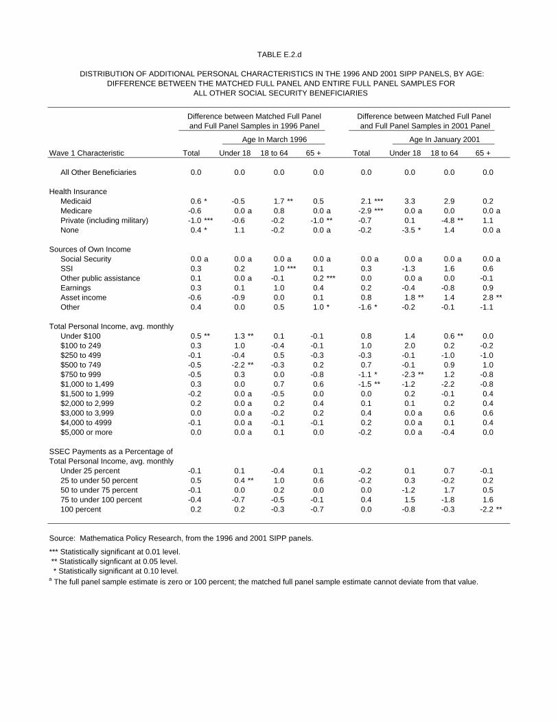
TABLE E.2.d

DISTRIBUTION OF ADDITIONAL PERSONAL CHARACTERISTICS IN THE 1996 AND 2001 SIPP PANELS, BY AGE:DIFFERENCE BETWEEN THE MATCHED FULL PANEL AND ENTIRE FULL PANEL SAMPLES FOR

ALL OTHER SOCIAL SECURITY BENEFICIARIES

Difference between Matched Full Panel Difference between Matched Full Paneland Full Panel Samples in 1996 Panel and Full Panel Samples in 2001 Panel

Age In March 1996 Age In January 2001

Wave 1 Characteristic Total Under 18 18 to 64 65 + Total Under 18 18 to 64 65 +

All Other Beneficiaries 0.0 0.0 0.0 0.0 0.0 0.0 0.0 0.0

Health InsuranceMedicaid 0.6 * -0.5 1.7 ** 0.5 2.1 *** 3.3 2.9 0.2 Medicare -0.6 0.0 a 0.8 0.0 a -2.9 *** 0.0 a 0.0 0.0 aPrivate (including military) -1.0 *** -0.6 -0.2 -1.0 ** -0.7 0.1 -4.8 ** 1.1 None 0.4 * 1.1 -0.2 0.0 a -0.2 -3.5 * 1.4 0.0 a

Sources of Own IncomeSocial Security 0.0 a 0.0 a 0.0 a 0.0 a 0.0 a 0.0 a 0.0 a 0.0 aSSI 0.3 0.2 1.0 *** 0.1 0.3 -1.3 1.6 0.6 Other public assistance 0.1 0.0 a -0.1 0.2 *** 0.0 0.0 a 0.0 -0.1 Earnings 0.3 0.1 1.0 0.4 0.2 -0.4 -0.8 0.9 Asset income -0.6 -0.9 0.0 0.1 0.8 1.8 ** 1.4 2.8 **Other 0.4 0.0 0.5 1.0 * -1.6 * -0.2 -0.1 -1.1

Total Personal Income, avg. monthlyUnder $100 0.5 ** 1.3 ** 0.1 -0.1 0.8 1.4 0.6 ** 0.0 $100 to 249 0.3 1.0 -0.4 -0.1 1.0 2.0 0.2 -0.2 $250 to 499 -0.1 -0.4 0.5 -0.3 -0.3 -0.1 -1.0 -1.0 $500 to 749 -0.5 -2.2 ** -0.3 0.2 0.7 -0.1 0.9 1.0 $750 to 999 -0.5 0.3 0.0 -0.8 -1.1 * -2.3 ** 1.2 -0.8 $1,000 to 1,499 0.3 0.0 0.7 0.6 -1.5 ** -1.2 -2.2 -0.8 $1,500 to 1,999 -0.2 0.0 a -0.5 0.0 0.0 0.2 -0.1 0.4 $2,000 to 2,999 0.2 0.0 a 0.2 0.4 0.1 0.1 0.2 0.4 $3,000 to 3,999 0.0 0.0 a -0.2 0.2 0.4 0.0 a 0.6 0.6 $4,000 to 4999 -0.1 0.0 a -0.1 -0.1 0.2 0.0 a 0.1 0.4 $5,000 or more 0.0 0.0 a 0.1 0.0 -0.2 0.0 a -0.4 0.0

SSEC Payments as a Percentage ofTotal Personal Income, avg. monthly

Under 25 percent -0.1 0.1 -0.4 0.1 -0.2 0.1 0.7 -0.1 25 to under 50 percent 0.5 0.4 ** 1.0 0.6 -0.2 0.3 -0.2 0.2 50 to under 75 percent -0.1 0.0 0.2 0.0 0.0 -1.2 1.7 0.5 75 to under 100 percent -0.4 -0.7 -0.5 -0.1 0.4 1.5 -1.8 1.6 100 percent 0.2 0.2 -0.3 -0.7 0.0 -0.8 -0.3 -2.2 **

Source: Mathematica Policy Research, from the 1996 and 2001 SIPP panels.

*** Statistically significant at 0.01 level. ** Statistically signficant at 0.05 level. * Statistically significant at 0.10 level.a The full panel sample estimate is zero or 100 percent; the matched full panel sample estimate cannot deviate from that value.

TABLE E.2.e

DISTRIBUTION OF ADDITIONAL PERSONAL CHARACTERISTICS IN THE 1996 AND 2001 SIPP PANELS, BY AGE:DIFFERENCE BETWEEN THE MATCHED FULL PANEL AND ENTIRE FULL PANEL SAMPLES FOR

SSI RECIPIENTS

Difference between Matched Full Panel Difference between Matched Full Paneland Full Panel Samples in 1996 Panel and Full Panel Samples in 2001 Panel

Age In March 1996 Age In January 2001

Wave 1 Characteristic Total Under 18 18 to 64 65 + Total Under 18 18 to 64 65 +

All SSI Recipients 0.0 0.0 0.0 0.0 0.0 0.0 0.0 0.0

Health InsuranceMedicaid 0.3 0.2 0.4 0.1 0.8 -1.5 1.4 ** 0.6 Medicare 0.4 0.0 a 0.3 2.4 ** 0.6 0.0 a 0.7 1.0 Private (including military) -0.5 -2.3 -0.4 -0.1 -1.0 -3.3 -0.6 -1.9 None -0.1 0.5 -0.3 0.0 -0.5 0.6 -0.6 -0.8 *

Sources of Own IncomeSocial Security 0.8 0.6 0.7 2.4 ** -0.2 -4.3 0.1 1.0 SSI 0.0 a 0.0 a 0.0 a 0.0 a 0.0 a 0.0 a 0.0 a 0.0 aOther public assistance 0.1 -0.8 0.0 0.5 0.6 0.3 0.8 0.4 Earnings 0.0 -0.8 0.0 0.1 0.1 -2.6 0.3 1.0 Asset income 0.1 0.1 0.0 0.3 0.8 -0.9 1.4 0.2 Other 0.0 0.0 a -0.3 0.5 -1.1 * 0.0 a -1.1 -1.3

Total Personal Income, avg. monthlyUnder $100 -0.1 -1.0 0.0 0.2 -0.1 0.7 -0.1 -0.3 $100 to 249 0.0 -0.1 0.1 -0.2 0.0 3.4 -1.0 ** 0.7 $250 to 499 0.5 0.5 0.9 -0.1 -0.7 -5.1 -1.5 3.3 $500 to 749 -0.7 -0.6 -0.6 -0.5 1.7 6.7 * 3.4 ** -4.9 *$750 to 999 0.5 ** 1.0 ** 0.3 0.4 * -0.2 -1.2 0.0 0.0 $1,000 to 1,499 -0.1 0.0 -0.3 0.4 *** -0.5 -4.8 * -0.5 1.9 **$1,500 to 1,999 0.0 0.0 a -0.1 0.1 0.2 0.2 0.2 0.1 $2,000 to 2,999 -0.2 0.0 a -0.3 -0.2 -0.2 0.0 a -0.2 -0.3 $3,000 to 3,999 0.0 0.0 a 0.0 0.0 a -0.3 0.0 a -0.3 -0.3 $4,000 to 4999 0.0 0.0 a 0.0 0.0 a 0.0 0.0 a 0.1 0.0 a$5,000 or more 0.0 0.0 a 0.0 0.0 a 0.0 0.0 a 0.0 a -0.2

SSEC Payments as a Percentage ofTotal Personal Income, avg. monthly

Under 25 percent -0.9 * -0.4 -0.9 -2.4 ** -0.1 4.5 -0.4 -1.6 25 to under 50 percent 0.4 ** 0.5 0.2 1.3 *** -1.1 ** -1.8 -0.8 -1.4 50 to under 75 percent 0.5 -0.5 0.6 ** 1.1 1.7 *** -2.3 1.4 ** 4.6 ***75 to under 100 percent 0.0 0.4 0.1 0.0 -0.6 -0.4 -0.2 -1.6 100 percent 0.0 a 0.0 a 0.0 a 0.0 a 0.0 a 0.0 a 0.0 a 0.0 a

Source: Mathematica Policy Research, from the 1996 and 2001 SIPP panels.

*** Statistically significant at 0.01 level. ** Statistically signficant at 0.05 level. * Statistically significant at 0.10 level.a The full panel sample estimate is zero or 100 percent; the matched full panel sample estimate cannot deviate from that value.

TABLE E.3.a

DISTRIBUTION OF HOUSEHOLD AND FAMILY CHARACTERISTICS IN THE 1996 AND 2001 SIPP PANELS, BY AGE:DIFFERENCE BETWEEN THE MATCHED FULL PANEL AND ENTIRE FULL PANEL SAMPLES FOR

THE TOTAL POPULATION

Difference between Matched Full Panel Difference between Matched Full Paneland Full Panel Samples in 1996 Panel and Full Panel Samples in 2001 Panel

Age In March 1996 Age In January 2001

Wave 1 Characteristic Total Under 18 18 to 64 65 + Total Under 18 18 to 64 65 +

All Persons 0.0 0.0 0.0 0.0 0.0 0.0 0.0 0.0

Household TypeFamily Married couple present 0.2 * 0.1 0.2 ** 0.0 -0.6 *** -1.8 *** -0.4 ** 1.0 * No married couple present Male householder -0.2 *** -0.3 *** -0.2 *** -0.1 0.1 0.3 -0.1 0.2 Female householder 0.1 * 0.3 * 0.1 0.0 0.6 *** 1.6 *** 0.3 ** 0.2 Nonfamily Male householder -0.1 *** -0.1 ** -0.2 *** 0.3 *** -0.1 0.0 -0.1 -0.3 Female householder 0.0 0.0 0.1 ** -0.2 0.0 0.0 0.2 ** -1.3 ***

Ownership Status of Living QuartersOwned 0.4 *** 0.3 0.5 *** 0.1 0.3 0.1 0.6 ** -0.3 Not owned -0.4 *** -0.3 -0.5 *** -0.1 -0.3 -0.1 -0.6 ** 0.3

Residence in Public Housing 0.1 ** 0.3 ** 0.1 0.2 *** 0.2 *** 0.4 *** 0.1 0.0

Household Size1 person 0.0 0.0 a 0.0 0.1 0.0 0.0 0.3 *** -1.6 ***2 persons 0.0 0.0 0.1 0.0 0.1 0.3 ** -0.2 1.1 **3 to 4 persons 0.1 0.1 0.0 0.0 0.4 0.8 0.3 0.5 5 or more persons -0.1 -0.1 -0.1 -0.1 -0.5 ** -1.1 ** -0.4 -0.1

Family Size1 person -0.1 ** -0.1 * -0.2 * 0.2 -0.1 0.0 0.1 -1.4 ***2 persons 0.0 0.0 0.0 0.0 0.2 0.5 *** 0.0 0.9 *3 to 4 persons 0.1 0.2 0.1 0.0 0.5 * 0.9 * 0.3 0.6 *5 or more persons 0.0 -0.1 0.1 -0.1 -0.6 ** -1.3 *** -0.4 * -0.1

Persons under 18 in FamilyNone -0.2 *** -0.1 -0.3 ** 0.0 0.1 0.0 0.1 0.2 1 person 0.0 -0.3 * 0.2 -0.1 -0.1 0.2 -0.1 -0.2 2 persons 0.0 -0.1 0.0 0.0 0.0 0.0 0.0 0.0 3 persons 0.1 0.2 0.1 0.0 0.1 0.1 0.0 0.0 4 persons 0.0 -0.1 0.1 0.0 0.0 0.1 0.0 0.1 5 or more persons 0.1 0.3 * 0.0 0.0 -0.2 -0.4 -0.1 ** 0.0

Source: Mathematica Policy Research, from the 1996 and 2001 SIPP panels.

*** Statistically significant at 0.01 level. ** Statistically signficant at 0.05 level. * Statistically significant at 0.10 level.a The full panel sample estimate is zero or 100 percent; the matched full panel sample estimate cannot deviate from that value.

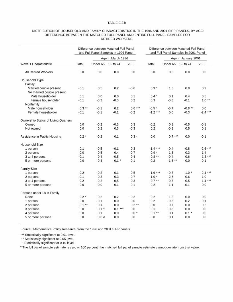
TABLE E.3.b

DISTRIBUTION OF HOUSEHOLD AND FAMILY CHARACTERISTICS IN THE 1996 AND 2001 SIPP PANELS, BY AGE:DIFFERENCE BETWEEN THE MATCHED FULL PANEL AND ENTIRE FULL PANEL SAMPLES FOR

RETIRED WORKERS

Difference between Matched Full Panel Difference between Matched Full Paneland Full Panel Samples in 1996 Panel and Full Panel Samples in 2001 Panel

Age In March 1996 Age In January 2001

Wave 1 Characteristic Total Under 65 65 to 74 75 + Total Under 65 65 to 74 75 +

All Retired Workers 0.0 0.0 0.0 0.0 0.0 0.0 0.0 0.0

Household TypeFamily Married couple present -0.1 0.5 0.2 -0.6 0.9 * 1.3 0.8 0.9 No married couple present Male householder 0.1 0.0 0.0 0.1 0.4 * 0.1 0.4 0.5 Female householder -0.1 -0.3 -0.3 0.2 0.3 -0.8 -0.1 1.0 **Nonfamily Male householder 0.3 ** -0.1 0.2 0.6 *** -0.5 * -0.7 -0.8 ** 0.0 Female householder -0.1 -0.1 -0.1 -0.2 -1.2 *** 0.0 -0.3 -2.4 ***

Ownership Status of Living QuartersOwned 0.0 -0.2 -0.3 0.3 -0.2 0.8 -0.5 -0.1 Not owned 0.0 0.2 0.3 -0.3 0.2 -0.8 0.5 0.1

Residence in Public Housing 0.2 * -0.2 0.1 0.3 * 0.0 0.7 *** 0.0 -0.1

Household Size1 person 0.1 -0.5 -0.1 0.3 -1.4 *** 0.4 -0.8 -2.6 ***2 persons 0.0 0.5 0.4 -0.7 0.9 * 1.5 0.3 1.4 3 to 4 persons -0.1 0.4 -0.5 0.4 0.8 ** -0.4 0.6 1.3 ***5 or more persons 0.0 -0.4 0.1 * -0.1 -0.2 -1.6 ** 0.0 -0.1

Family Size1 person 0.2 -0.2 0.1 0.5 -1.6 *** -0.8 -1.0 * -2.4 ***2 persons -0.1 0.3 0.3 -0.7 1.0 * 2.6 0.6 1.0 3 to 4 persons -0.2 -0.2 -0.5 0.3 0.7 ** -0.7 0.5 1.4 ***5 or more persons 0.0 0.0 0.1 -0.1 -0.2 -1.1 -0.1 0.0

Persons under 18 in FamilyNone -0.2 * -0.2 -0.2 -0.2 0.2 1.3 0.0 0.0 1 person 0.0 -0.1 0.0 0.0 -0.2 -0.5 -0.2 -0.1 2 persons 0.1 ** 0.1 0.0 0.2 ** 0.0 -0.7 0.0 0.2 3 persons 0.0 0.1 * 0.1 *** 0.0 -0.1 -0.3 0.0 0.0 4 persons 0.0 0.1 0.0 0.0 * 0.1 ** 0.1 0.1 * 0.0 5 or more persons 0.0 0.0 a 0.0 0.0 0.0 0.1 0.0 0.0

Source: Mathematica Policy Research, from the 1996 and 2001 SIPP panels.

*** Statistically significant at 0.01 level. ** Statistically signficant at 0.05 level. * Statistically significant at 0.10 level.a The full panel sample estimate is zero or 100 percent; the matched full panel sample estimate cannot deviate from that value.

TABLE E.3.c

DISTRIBUTION OF HOUSEHOLD AND FAMILY CHARACTERISTICS IN THE 1996 AND 2001 SIPP PANELS, BY AGE:DIFFERENCE BETWEEN THE MATCHED FULL PANEL AND ENTIRE FULL PANEL SAMPLES FOR

DISABLED WORKERS

Difference between Matched Full Panel Difference between Matched Full Paneland Full Panel Samples in 1996 Panel and Full Panel Samples in 2001 Panel

Age In March 1996 Age In January 2001

Wave 1 Characteristic Total Under 50 50 to 64 65 + Total Under 50 50 to 64 65 +

All Disabled Workers 0.0 0.0 0.0 0.0 0.0 0.0 0.0 0.0

Household TypeFamily Married couple present 0.3 0.2 -0.2 1.6 0.6 1.1 1.7 -1.1 No married couple present Male householder 0.4 0.4 0.3 0.3 -0.4 -0.3 -0.4 -0.5 Female householder -0.2 0.1 -0.1 -1.5 0.5 -1.3 1.0 1.5 Nonfamily Male householder -0.2 -0.4 0.0 -0.3 -0.1 0.6 -1.6 1.3 Female householder -0.3 -0.5 0.3 -0.5 -0.6 0.5 -0.8 -1.3

Ownership Status of Living QuartersOwned -1.0 * -1.8 * -0.7 0.7 -0.3 1.6 -2.3 1.2 Not owned 1.0 * 1.8 * 0.7 -0.7 0.3 -1.6 2.3 -1.2

Residence in Public Housing 0.5 ** 0.5 0.2 0.8 * 0.5 -0.3 1.4 ** 0.1

Household Size1 person -0.3 -0.9 0.3 0.1 -0.3 1.3 -0.9 -0.8 2 persons -0.6 0.9 -1.3 -0.2 -0.1 -2.3 2.6 0.1 3 to 4 persons 0.6 -0.8 1.3 0.7 0.1 0.3 -1.6 1.1 5 or more persons 0.3 0.9 -0.2 -0.5 0.3 0.8 -0.1 -0.4

Family Size1 person -0.2 -0.3 -0.1 0.0 -0.9 0.4 -2.5 0.1 2 persons -0.5 0.7 -0.9 -0.6 0.3 -1.5 3.3 ** -0.5 3 to 4 persons 0.6 -0.9 1.2 1.0 -0.1 0.1 -1.5 1.1 5 or more persons 0.1 0.5 -0.2 -0.4 0.6 1.0 0.7 -0.8

Persons under 18 in FamilyNone -0.4 -0.8 -0.2 1.1 -1.3 -1.6 -0.9 0.0 1 person 0.3 0.6 0.4 -0.8 0.2 0.4 -0.6 0.6 2 persons 0.3 0.2 0.2 0.4 * 0.9 ** 1.7 * 1.1 * -1.0 3 persons -0.3 -0.2 -0.4 -0.6 0.3 0.0 0.2 0.4 4 persons 0.1 0.1 0.0 0.1 * 0.3 ** 0.5 * 0.2 0.0 a5 or more persons 0.0 0.1 0.0 -0.2 -0.4 -1.0 -0.1 0.0 a

Source: Mathematica Policy Research, from the 1996 and 2001 SIPP panels.

*** Statistically significant at 0.01 level. ** Statistically signficant at 0.05 level. * Statistically significant at 0.10 level.a The full panel sample estimate is zero or 100 percent; the matched full panel sample estimate cannot deviate from that value.

TABLE E.3.d

DISTRIBUTION OF HOUSEHOLD AND FAMILY CHARACTERISTICS IN THE 1996 AND 2001 SIPP PANELS, BY AGE:DIFFERENCE BETWEEN THE MATCHED FULL PANEL AND ENTIRE FULL PANEL SAMPLES FOR

ALL OTHER SOCIAL SECURITY BENEFICIARIES

Difference between Matched Full Panel Difference between Matched Full Paneland Full Panel Samples in 1996 Panel and Full Panel Samples in 2001 Panel

Age In March 1996 Age In January 2001

Wave 1 Characteristic Total Under 18 18 to 64 65 + Total Under 18 18 to 64 65 +

All Other Beneficiaries 0.0 0.0 0.0 0.0 0.0 0.0 0.0 0.0

Household TypeFamily Married couple present 0.4 -0.5 -0.7 1.0 ** 0.9 1.0 -1.4 0.5 No married couple present Male householder -0.1 -0.3 0.4 -0.3 0.6 1.1 -0.1 0.3 Female householder 0.8 ** 0.7 0.2 0.5 0.7 -1.6 0.8 0.7 Nonfamily Male householder 0.1 0.1 -0.2 0.1 -0.2 -0.2 -0.2 -0.1 Female householder -1.2 *** 0.0 0.4 -1.4 *** -2.1 ** -0.2 0.8 -1.5

Ownership Status of Living QuartersOwned -0.2 0.4 -0.2 -0.2 -0.7 -0.9 -1.5 0.2 Not owned 0.2 -0.4 0.2 0.2 0.7 0.9 1.5 -0.2

Residence in Public Housing 0.0 -0.8 * -0.3 0.4 *** -0.3 -0.7 1.2 * -0.5

Household Size1 person -1.1 *** 0.0 a 0.0 -1.1 ** -2.5 *** 0.0 a 0.0 -2.1 2 persons -0.2 0.2 -0.6 0.2 -0.8 -1.2 -0.7 0.5 3 to 4 persons 0.8 ** 0.2 0.6 0.7 * 1.9 * -0.2 0.2 1.3 *5 or more persons 0.4 -0.4 0.0 0.3 1.5 * 1.4 0.5 0.3

Family Size1 person -1.3 *** -0.5 -0.1 -1.2 ** -2.0 * -0.1 1.4 -1.4 2 persons -0.1 -0.3 -0.5 0.4 -1.3 -1.4 -2.0 0.1 3 to 4 persons 0.9 ** 0.6 0.3 0.6 1.8 * 0.4 -0.2 1.1 5 or more persons 0.5 0.2 0.3 0.2 1.4 * 1.1 0.8 0.2

Persons under 18 in FamilyNone -1.1 ** -0.5 0.4 -0.5 * -2.6 ** -0.1 1.6 -0.7 1 person 0.0 -1.0 -0.7 0.3 * -0.3 -2.5 -3.2 0.2 2 persons 0.4 0.5 0.2 0.0 1.1 0.5 0.3 0.1 3 persons 0.4 0.4 0.3 0.1 ** 1.2 * 2.2 0.4 0.0 4 persons 0.2 0.1 -0.1 0.1 0.5 0.5 0.6 0.2 5 or more persons 0.1 0.5 -0.2 -0.1 0.1 -0.6 0.3 0.0

Source: Mathematica Policy Research, from the 1996 and 2001 SIPP panels.

*** Statistically significant at 0.01 level. ** Statistically signficant at 0.05 level. * Statistically significant at 0.10 level.a The full panel sample estimate is zero or 100 percent; the matched full panel sample estimate cannot deviate from that value.

TABLE E.3.e

DISTRIBUTION OF HOUSEHOLD AND FAMILY CHARACTERISTICS IN THE 1996 AND 2001 SIPP PANELS, BY AGE:DIFFERENCE BETWEEN THE MATCHED FULL PANEL AND ENTIRE FULL PANEL SAMPLES FOR

SSI RECIPIENTS

Difference between Matched Full Panel Difference between Matched Full Paneland Full Panel Samples in 1996 Panel and Full Panel Samples in 2001 Panel

Age In March 1996 Age In January 2001

Wave 1 Characteristic Total Under 18 18 to 64 65 + Total Under 18 18 to 64 65 +

All SSI Recipients 0.0 0.0 0.0 0.0 0.0 0.0 0.0 0.0

Household TypeFamily Married couple present 0.0 -0.2 0.2 -0.4 1.1 3.6 0.6 0.9 No married couple present Male householder -0.6 -0.3 -0.1 -1.8 ** -0.1 -0.6 0.2 -0.5 Female householder 0.8 0.8 0.5 0.9 -1.2 -3.0 -1.3 -0.4 Nonfamily Male householder 0.1 -0.3 0.0 0.4 0.5 0.0 a 0.8 0.2 Female householder -0.2 0.0 a -0.3 0.8 -0.2 0.0 a 0.2 -1.1

Ownership Status of Living QuartersOwned -0.1 -0.5 0.6 -1.2 0.2 4.7 0.2 -2.0 Not owned 0.1 0.5 -0.6 1.2 -0.2 -4.7 -0.2 2.0

Residence in Public Housing 0.4 1.3 -0.1 1.0 0.8 -0.4 0.8 1.4

Household Size1 person -0.2 0.0 a -0.7 1.3 1.2 0.0 a 2.0 ** 0.0 2 persons 0.1 -0.6 0.4 0.4 -1.5 -0.9 -2.6 ** 2.0 3 to 4 persons 0.1 0.7 -0.1 -0.5 -0.3 -0.6 -0.2 -0.9 5 or more persons 0.0 0.0 0.4 -1.2 0.6 1.5 0.9 -1.1

Family Size1 person 0.2 0.6 -0.1 1.4 0.3 0.8 0.5 0.3 2 persons 0.2 -1.4 0.6 0.5 -0.1 -0.4 -0.4 1.0 3 to 4 persons -0.2 0.6 -0.5 -0.6 -0.4 -1.5 -0.6 0.1 5 or more persons -0.2 0.2 0.0 -1.3 0.3 1.1 0.5 -1.4

Persons under 18 in FamilyNone 0.5 0.6 0.8 0.9 -0.6 0.8 -1.0 1.8 1 person -0.7 * -2.4 -0.6 -0.6 -0.2 0.6 -0.4 -0.8 2 persons 0.0 1.1 -0.3 -0.4 0.3 0.8 0.5 -1.1 3 persons 0.3 0.7 0.1 0.3 0.5 -2.8 1.2 ** -0.2 4 persons 0.0 0.6 -0.2 0.0 0.2 0.9 0.0 0.2 5 or more persons 0.0 -0.6 0.1 ** -0.3 -0.2 -0.2 -0.3 0.1

Source: Mathematica Policy Research, from the 1996 and 2001 SIPP panels.

*** Statistically significant at 0.01 level. ** Statistically signficant at 0.05 level. * Statistically significant at 0.10 level.a The full panel sample estimate is zero or 100 percent; the matched full panel sample estimate cannot deviate from that value.

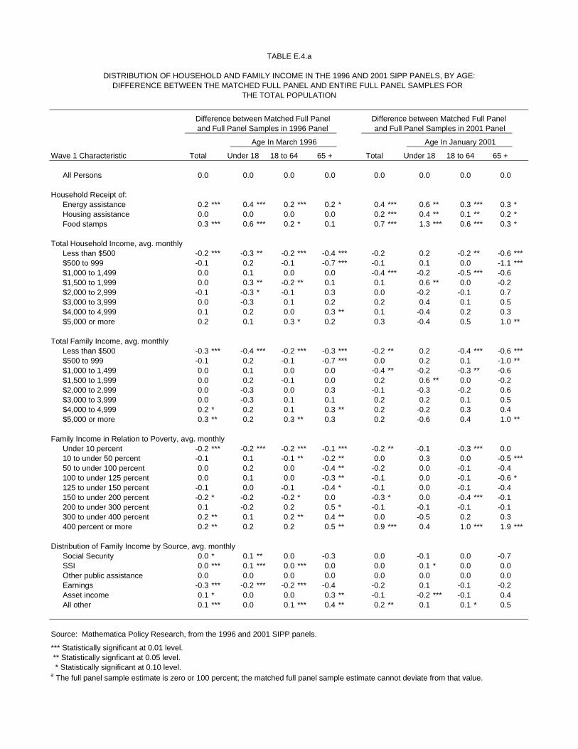
TABLE E.4.a

DISTRIBUTION OF HOUSEHOLD AND FAMILY INCOME IN THE 1996 AND 2001 SIPP PANELS, BY AGE:DIFFERENCE BETWEEN THE MATCHED FULL PANEL AND ENTIRE FULL PANEL SAMPLES FOR

THE TOTAL POPULATION

Difference between Matched Full Panel Difference between Matched Full Paneland Full Panel Samples in 1996 Panel and Full Panel Samples in 2001 Panel

Age In March 1996 Age In January 2001

Wave 1 Characteristic Total Under 18 18 to 64 65 + Total Under 18 18 to 64 65 +

All Persons 0.0 0.0 0.0 0.0 0.0 0.0 0.0 0.0

Household Receipt of:Energy assistance 0.2 *** 0.4 *** 0.2 *** 0.2 * 0.4 *** 0.6 ** 0.3 *** 0.3 *Housing assistance 0.0 0.0 0.0 0.0 0.2 *** 0.4 ** 0.1 ** 0.2 *Food stamps 0.3 *** 0.6 *** 0.2 * 0.1 0.7 *** 1.3 *** 0.6 *** 0.3 *

Total Household Income, avg. monthlyLess than $500 -0.2 *** -0.3 ** -0.2 *** -0.4 *** -0.2 0.2 -0.2 ** -0.6 ***$500 to 999 -0.1 0.2 -0.1 -0.7 *** -0.1 0.1 0.0 -1.1 ***$1,000 to 1,499 0.0 0.1 0.0 0.0 -0.4 *** -0.2 -0.5 *** -0.6 $1,500 to 1,999 0.0 0.3 ** -0.2 ** 0.1 0.1 0.6 ** 0.0 -0.2 $2,000 to 2,999 -0.1 -0.3 * -0.1 0.3 0.0 -0.2 -0.1 0.7 $3,000 to 3,999 0.0 -0.3 0.1 0.2 0.2 0.4 0.1 0.5 $4,000 to 4,999 0.1 0.2 0.0 0.3 ** 0.1 -0.4 0.2 0.3 $5,000 or more 0.2 0.1 0.3 * 0.2 0.3 -0.4 0.5 1.0 **

Total Family Income, avg. monthlyLess than $500 -0.3 *** -0.4 *** -0.2 *** -0.3 *** -0.2 ** 0.2 -0.4 *** -0.6 ***$500 to 999 -0.1 0.2 -0.1 -0.7 *** 0.0 0.2 0.1 -1.0 **$1,000 to 1,499 0.0 0.1 0.0 0.0 -0.4 ** -0.2 -0.3 ** -0.6 $1,500 to 1,999 0.0 0.2 -0.1 0.0 0.2 0.6 ** 0.0 -0.2 $2,000 to 2,999 0.0 -0.3 0.0 0.3 -0.1 -0.3 -0.2 0.6 $3,000 to 3,999 0.0 -0.3 0.1 0.1 0.2 0.2 0.1 0.5 $4,000 to 4,999 0.2 * 0.2 0.1 0.3 ** 0.2 -0.2 0.3 0.4 $5,000 or more 0.3 ** 0.2 0.3 ** 0.3 0.2 -0.6 0.4 1.0 **

Family Income in Relation to Poverty, avg. monthlyUnder 10 percent -0.2 *** -0.2 *** -0.2 *** -0.1 *** -0.2 ** -0.1 -0.3 *** 0.0 10 to under 50 percent -0.1 0.1 -0.1 ** -0.2 ** 0.0 0.3 0.0 -0.5 ***50 to under 100 percent 0.0 0.2 0.0 -0.4 ** -0.2 0.0 -0.1 -0.4 100 to under 125 percent 0.0 0.1 0.0 -0.3 ** -0.1 0.0 -0.1 -0.6 *125 to under 150 percent -0.1 0.0 -0.1 -0.4 * -0.1 0.0 -0.1 -0.4 150 to under 200 percent -0.2 * -0.2 -0.2 * 0.0 -0.3 * 0.0 -0.4 *** -0.1 200 to under 300 percent 0.1 -0.2 0.2 0.5 * -0.1 -0.1 -0.1 -0.1 300 to under 400 percent 0.2 ** 0.1 0.2 ** 0.4 ** 0.0 -0.5 0.2 0.3 400 percent or more 0.2 ** 0.2 0.2 0.5 ** 0.9 *** 0.4 1.0 *** 1.9 ***

Distribution of Family Income by Source, avg. monthlySocial Security 0.0 * 0.1 ** 0.0 -0.3 0.0 -0.1 0.0 -0.7 SSI 0.0 *** 0.1 *** 0.0 *** 0.0 0.0 0.1 * 0.0 0.0 Other public assistance 0.0 0.0 0.0 0.0 0.0 0.0 0.0 0.0 Earnings -0.3 *** -0.2 *** -0.2 *** -0.4 -0.2 0.1 -0.1 -0.2 Asset income 0.1 * 0.0 0.0 0.3 ** -0.1 -0.2 *** -0.1 0.4 All other 0.1 *** 0.0 0.1 *** 0.4 ** 0.2 ** 0.1 0.1 * 0.5

Source: Mathematica Policy Research, from the 1996 and 2001 SIPP panels.

*** Statistically significant at 0.01 level. ** Statistically signficant at 0.05 level. * Statistically significant at 0.10 level.a The full panel sample estimate is zero or 100 percent; the matched full panel sample estimate cannot deviate from that value.

TABLE E.4.b

DISTRIBUTION OF HOUSEHOLD AND FAMILY INCOME IN THE 1996 AND 2001 SIPP PANELS, BY AGE:DIFFERENCE BETWEEN THE MATCHED FULL PANEL AND ENTIRE FULL PANEL SAMPLES FOR

RETIRED WORKERS

Difference between Matched Full Panel Difference between Matched Full Paneland Full Panel Samples in 1996 Panel and Full Panel Samples in 2001 Panel

Age In March 1996 Age In January 2001

Wave 1 Characteristic Total Under 65 65 to 74 75 + Total Under 65 65 to 74 75 +

All Retired Workers 0.0 0.0 0.0 0.0 0.0 0.0 0.0 0.0

Household Receipt of:Energy assistance 0.1 * 0.0 0.1 0.2 0.3 * 0.1 0.3 0.4 Housing assistance 0.0 -0.1 0.1 0.0 0.1 0.0 0.1 0.2 Food stamps 0.1 0.1 0.2 0.1 0.4 ** -0.3 0.7 *** 0.3

Total Household Income, avg. monthlyLess than $500 -0.2 * -0.3 -0.3 ** -0.1 -0.6 *** -0.4 -0.2 -1.0 ***$500 to 999 -0.8 *** -0.7 -0.6 ** -1.0 ** -1.1 *** -1.1 -0.3 -2.1 ***$1,000 to 1,499 0.0 1.0 ** 0.4 -0.7 -0.3 1.2 -0.4 -0.6 $1,500 to 1,999 0.2 0.3 0.0 0.4 0.0 -0.4 -0.7 0.9 $2,000 to 2,999 0.1 0.8 0.1 -0.1 0.8 * 0.5 0.5 1.3 *$3,000 to 3,999 0.2 -0.1 0.0 0.5 * 0.5 1.3 0.7 0.0 $4,000 to 4,999 0.4 *** 0.0 0.3 * 0.5 ** 0.2 -0.4 -0.1 0.8 *$5,000 or more 0.1 -1.0 0.1 0.5 * 0.4 -0.6 0.5 0.7

Total Family Income, avg. monthlyLess than $500 -0.2 -0.3 -0.2 -0.2 -0.6 *** -0.6 -0.4 * -1.0 ***$500 to 999 -0.7 *** -0.8 -0.6 ** -0.9 ** -1.1 *** -1.2 -0.4 -1.9 **$1,000 to 1,499 0.1 1.1 *** 0.3 -0.5 -0.3 0.7 -0.3 -0.6 $1,500 to 1,999 0.1 0.3 -0.1 0.2 0.0 -0.4 -0.7 0.9 $2,000 to 2,999 0.2 0.8 0.3 -0.1 0.8 0.2 0.7 1.0 $3,000 to 3,999 0.1 0.0 -0.1 0.4 0.4 1.4 0.8 -0.2 $4,000 to 4,999 0.4 *** -0.1 0.3 * 0.5 *** 0.4 0.3 -0.1 0.9 **$5,000 or more 0.1 -1.1 0.1 0.5 ** 0.5 -0.4 0.4 0.8

Family Income in Relation to Poverty, avg. monthlyUnder 10 percent 0.0 0.0 0.0 0.0 0.0 -0.1 0.0 -0.1 10 to under 50 percent 0.0 0.1 -0.1 0.0 -0.4 *** -0.5 -0.3 ** -0.6 **50 to under 100 percent -0.5 *** -0.6 -0.3 -0.7 * -0.3 -0.7 0.1 -0.7 100 to under 125 percent -0.3 * 0.2 -0.2 -0.5 * -0.5 * 0.5 -0.3 -1.0 *125 to under 150 percent -0.4 * 0.4 -0.3 -0.8 * -0.3 0.1 0.1 -0.8 150 to under 200 percent 0.0 0.5 0.1 -0.1 -0.2 -1.2 -0.6 0.6 200 to under 300 percent 0.3 0.4 0.1 0.6 0.1 -0.3 -0.1 0.5 300 to under 400 percent 0.4 * 0.3 0.5 ** 0.3 0.3 -0.4 0.7 0.1 400 percent or more 0.5 * -1.1 0.2 1.2 *** 1.3 *** 2.7 ** 0.5 2.0 ***

Distribution of Family Income by Source, avg. monthlySocial Security -0.4 0.8 -0.4 -1.0 *** -0.6 -0.2 -0.1 -1.6 **SSI 0.0 0.0 0.0 0.0 0.0 -0.1 0.0 0.0 Other public assistance 0.0 0.0 0.0 ** 0.0 0.0 0.0 0.0 0.0 Earnings -0.3 -1.5 -0.4 0.3 -0.4 -1.0 -1.4 1.3 Asset income 0.4 *** 0.2 0.3 0.7 *** 0.5 0.1 0.7 0.2 All other 0.3 0.5 0.5 * 0.0 0.6 1.2 0.8 0.2

Source: Mathematica Policy Research, from the 1996 and 2001 SIPP panels.

*** Statistically significant at 0.01 level. ** Statistically signficant at 0.05 level. * Statistically significant at 0.10 level.a The full panel sample estimate is zero or 100 percent; the matched full panel sample estimate cannot deviate from that value.

TABLE E.4.c

DISTRIBUTION OF HOUSEHOLD AND FAMILY INCOME IN THE 1996 AND 2001 SIPP PANELS, BY AGE:DIFFERENCE BETWEEN THE MATCHED FULL PANEL AND ENTIRE FULL PANEL SAMPLES FOR

DISABLED WORKERS

Difference between Matched Full Panel Difference between Matched Full Paneland Full Panel Samples in 1996 Panel and Full Panel Samples in 2001 Panel

Age In March 1996 Age In January 2001

Wave 1 Characteristic Total Under 50 50 to 64 65 + Total Under 50 50 to 64 65 +

All Disabled Workers 0.0 0.0 0.0 0.0 0.0 0.0 0.0 0.0

Household Receipt of:Energy assistance 0.3 0.2 0.3 0.3 0.4 0.2 0.6 0.1 Housing assistance 0.2 0.3 0.1 0.0 0.8 * 0.6 1.2 ** 0.4 Food stamps 0.4 0.2 1.3 ** -1.0 1.0 -1.9 3.0 *** 1.4

Total Household Income, avg. monthlyLess than $500 0.3 0.1 0.5 0.3 -0.6 * -0.6 -1.0 * 0.1 $500 to 999 -0.4 0.1 -0.1 -1.4 0.8 -0.2 1.3 1.9 $1,000 to 1,499 -0.5 -0.8 -1.0 0.7 -1.5 * -0.5 -1.5 -2.8 $1,500 to 1,999 -0.3 -0.6 -0.5 0.6 1.2 2.8 ** 0.9 -0.8 $2,000 to 2,999 0.0 -0.9 0.7 -0.1 0.8 0.7 -0.4 2.8 $3,000 to 3,999 0.1 0.7 * -0.5 -0.1 -0.7 -1.9 0.7 -1.2 $4,000 to 4,999 0.4 0.5 *** 0.9 ** -0.6 0.5 0.9 0.3 0.6 $5,000 or more 0.5 * 0.8 0.0 0.6 -0.6 -1.1 -0.2 -0.5

Total Family Income, avg. monthlyLess than $500 0.4 0.2 0.7 * 0.4 -0.5 -0.4 -1.0 * 0.1 $500 to 999 -0.3 0.7 -0.5 -1.5 0.6 -0.5 0.5 2.3 $1,000 to 1,499 -0.8 -0.8 -1.4 0.1 -1.0 0.6 -1.8 -2.4 $1,500 to 1,999 -0.1 -0.9 0.0 1.1 1.0 2.4 ** 1.1 -1.1 $2,000 to 2,999 -0.4 -0.9 0.2 -0.6 0.5 0.5 -0.7 2.4 $3,000 to 3,999 0.4 0.8 ** 0.2 0.2 -0.5 -2.1 * 1.2 -0.8 $4,000 to 4,999 0.3 0.5 *** 0.8 ** -0.6 0.7 1.2 0.6 0.4 $5,000 or more 0.4 0.6 0.0 0.8 *** -0.8 -1.7 0.0 -0.9

Family Income in Relation to Poverty, avg. monthlyUnder 10 percent 0.0 a 0.0 a 0.0 a 0.0 a 0.1 0.0 a 0.1 0.2 10 to under 50 percent 0.0 0.3 * 0.2 -0.6 0.0 0.2 -0.4 0.0 50 to under 100 percent 0.2 0.1 0.3 -0.2 0.6 -0.6 0.3 2.4 100 to under 125 percent 0.0 0.4 0.0 -0.6 -0.4 0.1 0.0 -2.0 125 to under 150 percent -0.7 0.3 -1.8 ** -0.5 0.4 1.8 * -0.7 0.0 150 to under 200 percent 0.1 -0.6 0.4 0.9 0.1 0.7 -0.1 -0.5 200 to under 300 percent -0.1 -1.4 0.7 0.5 -0.5 -0.3 -1.3 0.8 300 to under 400 percent 0.3 0.3 -0.2 0.8 -0.2 -1.5 1.0 -0.7 400 percent or more 0.3 0.6 0.4 -0.3 0.1 -0.4 0.9 -0.1

Distribution of Family Income by Source, avg. monthlySocial Security -1.3 *** -1.7 ** -0.9 -1.1 0.3 1.5 -0.8 0.6 SSI 0.1 0.0 0.1 0.3 -0.2 -0.4 -0.1 0.1 Other public assistance 0.0 0.0 0.0 0.0 0.1 * 0.1 0.1 0.2 *Earnings 1.3 * 2.0 0.8 0.5 1.1 1.0 1.8 -0.2 Asset income 0.2 0.1 0.2 0.4 0.3 0.1 0.3 0.6 All other -0.2 -0.4 0.0 -0.1 -1.7 * -2.3 -1.3 -1.4

Source: Mathematica Policy Research, from the 1996 and 2001 SIPP panels.

*** Statistically significant at 0.01 level. ** Statistically signficant at 0.05 level. * Statistically significant at 0.10 level.a The full panel sample estimate is zero or 100 percent; the matched full panel sample estimate cannot deviate from that value.

TABLE E.4.d

DISTRIBUTION OF HOUSEHOLD AND FAMILY INCOME IN THE 1996 AND 2001 SIPP PANELS, BY AGE:DIFFERENCE BETWEEN THE MATCHED FULL PANEL AND ENTIRE FULL PANEL SAMPLES FOR

ALL OTHER SOCIAL SECURITY BENEFICIARIES

Difference between Matched Full Panel Difference between Matched Full Paneland Full Panel Samples in 1996 Panel and Full Panel Samples in 2001 Panel

Age In March 1996 Age In January 2001

Wave 1 Characteristic Total Under 18 18 to 64 65 + Total Under 18 18 to 64 65 +

All Other Beneficiaries 0.0 0.0 0.0 0.0 0.0 0.0 0.0 0.0

Household Receipt of:Energy assistance 0.0 -0.2 0.3 0.0 1.5 *** 2.8 ** 2.1 ** 0.4 Housing assistance -0.1 0.0 -1.0 0.0 0.4 1.3 * 0.0 0.1 Food stamps 0.4 0.0 -0.2 0.4 * 1.2 ** 2.0 2.2 ** 0.3

Total Household Income, avg. monthlyLess than $500 -0.4 -0.1 -0.2 -0.4 -0.7 ** -0.1 0.2 -1.1 *$500 to 999 -0.9 ** 0.5 -0.6 -1.4 ** 0.1 0.0 2.3 * 0.2 $1,000 to 1,499 0.3 0.3 1.4 ** 0.0 -1.7 ** -0.5 0.0 -2.4 **$1,500 to 1,999 0.1 0.2 -0.2 0.1 -0.1 1.1 0.6 -0.7 $2,000 to 2,999 0.6 0.0 -0.1 0.9 ** 0.8 1.9 -0.6 0.3 $3,000 to 3,999 0.8 *** 1.4 *** 0.5 0.5 ** 1.1 -0.4 3.2 ** 0.7 $4,000 to 4,999 -0.4 * -0.9 -0.1 -0.3 0.0 0.1 -2.5 * 0.5 $5,000 or more -0.1 -1.3 -0.9 0.5 0.6 -2.2 -3.1 2.4 **

Total Family Income, avg. monthlyLess than $500 -0.5 * -0.6 -0.5 -0.4 -0.8 * -0.5 0.3 -1.2 **$500 to 999 -0.8 ** 0.7 -0.3 -1.4 ** 0.4 0.4 2.3 0.6 $1,000 to 1,499 0.3 0.4 1.2 0.1 -2.1 *** -0.8 -1.0 -2.6 **$1,500 to 1,999 0.0 0.0 -0.5 0.2 -0.1 0.5 0.1 -0.4 $2,000 to 2,999 0.6 * 0.1 0.1 1.0 ** 1.2 2.7 0.6 0.3 $3,000 to 3,999 0.7 *** 1.3 *** 0.4 0.4 1.0 0.0 3.2 ** 0.4 $4,000 to 4,999 -0.3 -0.7 0.1 -0.3 -0.1 -0.1 -2.6 * 0.4 $5,000 or more -0.1 -1.2 -0.6 0.5 0.6 -2.2 -2.9 2.4 **

Family Income in Relation to Poverty, avg. monthlyUnder 10 percent 0.0 0.0 0.0 a 0.0 -0.2 -0.8 0.0 a 0.0 a10 to under 50 percent -0.2 0.5 -0.7 -0.4 * 0.0 0.9 ** 0.7 -0.6 50 to under 100 percent -0.2 0.1 -0.5 -0.4 0.7 1.0 2.1 0.1 100 to under 125 percent -0.2 -0.2 0.2 -0.3 0.6 1.2 1.7 0.1 125 to under 150 percent 0.0 0.4 0.4 -0.3 -0.8 0.7 -1.2 -1.3 *150 to under 200 percent 0.2 0.4 1.2 ** -0.1 -1.1 -2.7 0.1 -0.8 200 to under 300 percent 0.5 0.0 0.4 0.8 -0.1 1.3 -0.5 -0.6 300 to under 400 percent 0.4 -0.2 0.4 0.7 * -0.7 -1.6 0.5 -0.7 400 percent or more -0.6 -1.2 -1.3 * 0.0 1.5 0.1 -3.5 3.9 ***

Distribution of Family Income by Source, avg. monthlySocial Security 0.1 1.2 0.7 -0.8 ** -1.2 * -0.2 0.4 -1.9 *SSI 0.1 *** 0.1 0.4 *** 0.1 0.0 -0.5 0.5 0.1 Other public assistance 0.0 0.0 -0.3 ** 0.0 0.0 0.1 0.0 0.0 Earnings -0.1 -1.6 -1.3 1.2 ** 1.6 1.2 -3.4 2.5 Asset income -0.1 -0.1 0.1 -0.4 -0.2 -0.3 1.1 -0.3 All other 0.1 0.3 0.3 -0.2 -0.2 -0.3 1.3 -0.3

Source: Mathematica Policy Research, from the 1996 and 2001 SIPP panels.

*** Statistically significant at 0.01 level. ** Statistically signficant at 0.05 level. * Statistically significant at 0.10 level.a The full panel sample estimate is zero or 100 percent; the matched full panel sample estimate cannot deviate from that value.

TABLE E.4.e

DISTRIBUTION OF HOUSEHOLD AND FAMILY INCOME IN THE 1996 AND 2001 SIPP PANELS, BY AGE:DIFFERENCE BETWEEN THE MATCHED FULL PANEL AND ENTIRE FULL PANEL SAMPLES FOR

SSI RECIPIENTS

Difference between Matched Full Panel Difference between Matched Full Paneland Full Panel Samples in 1996 Panel and Full Panel Samples in 2001 Panel

Age In March 1996 Age In January 2001

Wave 1 Characteristic Total Under 18 18 to 64 65 + Total Under 18 18 to 64 65 +

All SSI Recipients 0.0 0.0 0.0 0.0 0.0 0.0 0.0 0.0

Household Receipt of:Energy assistance 0.6 ** 0.5 0.6 0.7 0.6 -0.1 1.4 -1.2 Housing assistance -0.3 -2.0 -0.3 0.4 1.0 0.8 1.2 0.7 Food stamps -0.3 -1.8 -0.1 0.0 1.6 2.6 2.3 -0.5

Total Household Income, avg. monthlyLess than $500 -0.2 -0.5 -0.3 0.7 0.2 1.1 0.0 0.4 $500 to 999 -0.1 -0.3 -0.4 0.8 -0.5 -3.4 1.0 -2.6 $1,000 to 1,499 -0.4 -0.5 -0.2 -0.9 0.1 -1.0 -0.4 2.3 *$1,500 to 1,999 0.4 0.9 0.4 0.1 0.5 -0.4 0.8 0.2 $2,000 to 2,999 0.6 1.0 0.4 0.5 -0.6 -2.0 -0.2 -1.4 $3,000 to 3,999 -0.2 -1.1 -0.1 -0.2 0.9 7.8 *** -0.4 1.1 $4,000 to 4,999 0.3 0.0 0.2 0.6 -0.7 -0.6 -0.5 -1.1 $5,000 or more -0.4 0.4 -0.1 -1.6 * 0.0 -1.4 -0.2 1.1

Total Family Income, avg. monthlyLess than $500 0.3 -0.4 0.4 0.8 0.4 1.8 0.1 0.4 $500 to 999 -0.1 0.4 -0.5 0.7 -0.8 -4.1 * 0.7 -2.5 $1,000 to 1,499 -0.3 -0.8 -0.2 -0.4 0.5 -0.2 0.0 2.3 *$1,500 to 1,999 0.3 0.3 0.4 0.1 -0.2 0.1 -0.4 0.2 $2,000 to 2,999 0.5 0.9 0.3 0.4 -0.3 -2.1 0.2 -1.3 $3,000 to 3,999 -0.2 -1.1 -0.1 -0.2 1.0 6.5 *** -0.2 1.3 $4,000 to 4,999 0.2 0.4 0.1 0.3 -0.5 -0.6 -0.2 -1.4 $5,000 or more -0.7 * 0.3 -0.4 -1.7 * -0.1 -1.4 -0.3 0.9

Family Income in Relation to Poverty, avg. monthlyUnder 10 percent 0.0 0.0 0.0 0.1 0.0 a 0.0 a 0.0 a 0.0 a10 to under 50 percent 0.0 -0.5 0.2 -0.2 0.0 -1.1 0.5 -1.0 50 to under 100 percent -0.3 -0.9 -0.7 1.1 -1.0 -1.4 -0.7 -0.9 100 to under 125 percent 0.5 2.3 *** 0.6 -0.4 0.4 -0.8 1.3 * -1.9 125 to under 150 percent 0.2 -0.6 0.3 0.3 1.1 * 0.4 1.0 1.8 150 to under 200 percent 0.3 1.0 0.0 0.4 -0.1 3.3 -1.0 0.8 200 to under 300 percent 0.0 -1.7 0.2 0.2 0.0 2.0 -0.8 1.1 300 to under 400 percent -0.2 0.4 -0.2 -0.4 0.2 -1.9 0.8 -0.7 400 percent or more -0.5 * 0.0 a -0.4 -1.1 -0.6 -0.6 -1.1 0.8

Distribution of Family Income by Source, avg. monthlySocial Security 0.6 0.3 0.5 1.8 0.1 -1.7 0.7 -0.7 SSI 0.6 0.9 0.5 0.2 0.7 0.5 1.8 -1.9 Other public assistance 0.0 -0.4 -0.1 0.5 0.3 * 0.5 0.3 * 0.0 Earnings -1.4 -1.2 -0.8 -2.8 0.4 2.0 -1.7 4.6 Asset income 0.0 0.1 0.0 0.1 -0.2 -2.1 0.1 0.2 All other 0.1 0.4 0.0 0.3 -1.3 * 0.8 -1.3 -2.3 **

Source: Mathematica Policy Research, from the 1996 and 2001 SIPP panels.

*** Statistically significant at 0.01 level. ** Statistically signficant at 0.05 level. * Statistically significant at 0.10 level.a The full panel sample estimate is zero or 100 percent; the matched full panel sample estimate cannot deviate from that value.

F-1

APPENDIX F

COMPARISON OF FULL PANEL AND CROSS-SECTION SAMPLES: 2001 SIPP PANEL

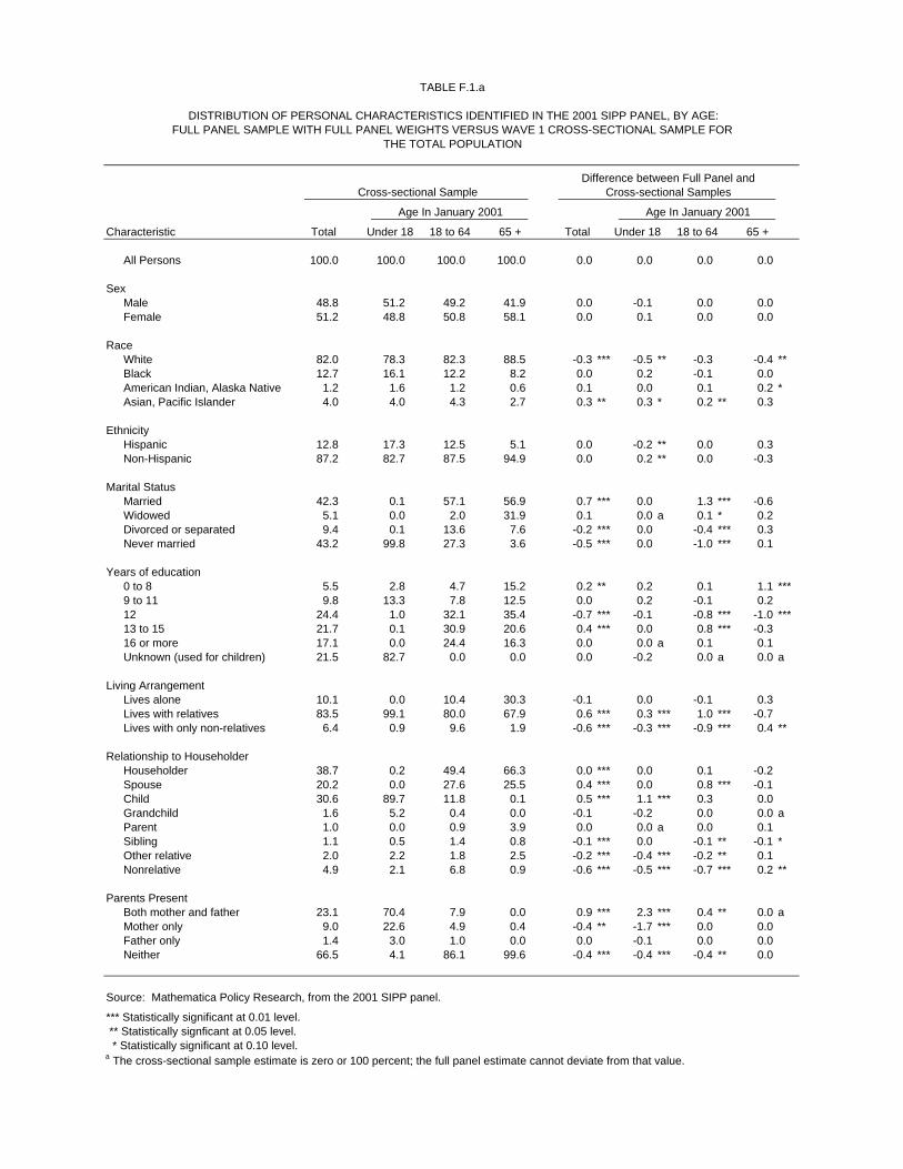
TABLE F.1.a

DISTRIBUTION OF PERSONAL CHARACTERISTICS IDENTIFIED IN THE 2001 SIPP PANEL, BY AGE:FULL PANEL SAMPLE WITH FULL PANEL WEIGHTS VERSUS WAVE 1 CROSS-SECTIONAL SAMPLE FOR

THE TOTAL POPULATION

Difference between Full Panel and Cross-sectional Sample Cross-sectional Samples

Age In January 2001 Age In January 2001

Characteristic Total Under 18 18 to 64 65 + Total Under 18 18 to 64 65 +

All Persons 100.0 100.0 100.0 100.0 0.0 0.0 0.0 0.0

SexMale 48.8 51.2 49.2 41.9 0.0 -0.1 0.0 0.0 Female 51.2 48.8 50.8 58.1 0.0 0.1 0.0 0.0

RaceWhite 82.0 78.3 82.3 88.5 -0.3 *** -0.5 ** -0.3 -0.4 **Black 12.7 16.1 12.2 8.2 0.0 0.2 -0.1 0.0 American Indian, Alaska Native 1.2 1.6 1.2 0.6 0.1 0.0 0.1 0.2 *Asian, Pacific Islander 4.0 4.0 4.3 2.7 0.3 ** 0.3 * 0.2 ** 0.3

EthnicityHispanic 12.8 17.3 12.5 5.1 0.0 -0.2 ** 0.0 0.3 Non-Hispanic 87.2 82.7 87.5 94.9 0.0 0.2 ** 0.0 -0.3

Marital StatusMarried 42.3 0.1 57.1 56.9 0.7 *** 0.0 1.3 *** -0.6 Widowed 5.1 0.0 2.0 31.9 0.1 0.0 a 0.1 * 0.2 Divorced or separated 9.4 0.1 13.6 7.6 -0.2 *** 0.0 -0.4 *** 0.3 Never married 43.2 99.8 27.3 3.6 -0.5 *** 0.0 -1.0 *** 0.1

Years of education0 to 8 5.5 2.8 4.7 15.2 0.2 ** 0.2 0.1 1.1 ***9 to 11 9.8 13.3 7.8 12.5 0.0 0.2 -0.1 0.2 12 24.4 1.0 32.1 35.4 -0.7 *** -0.1 -0.8 *** -1.0 ***13 to 15 21.7 0.1 30.9 20.6 0.4 *** 0.0 0.8 *** -0.3 16 or more 17.1 0.0 24.4 16.3 0.0 0.0 a 0.1 0.1 Unknown (used for children) 21.5 82.7 0.0 0.0 0.0 -0.2 0.0 a 0.0 a

Living ArrangementLives alone 10.1 0.0 10.4 30.3 -0.1 0.0 -0.1 0.3 Lives with relatives 83.5 99.1 80.0 67.9 0.6 *** 0.3 *** 1.0 *** -0.7 Lives with only non-relatives 6.4 0.9 9.6 1.9 -0.6 *** -0.3 *** -0.9 *** 0.4 **

Relationship to HouseholderHouseholder 38.7 0.2 49.4 66.3 0.0 *** 0.0 0.1 -0.2 Spouse 20.2 0.0 27.6 25.5 0.4 *** 0.0 0.8 *** -0.1 Child 30.6 89.7 11.8 0.1 0.5 *** 1.1 *** 0.3 0.0 Grandchild 1.6 5.2 0.4 0.0 -0.1 -0.2 0.0 0.0 aParent 1.0 0.0 0.9 3.9 0.0 0.0 a 0.0 0.1 Sibling 1.1 0.5 1.4 0.8 -0.1 *** 0.0 -0.1 ** -0.1 *Other relative 2.0 2.2 1.8 2.5 -0.2 *** -0.4 *** -0.2 ** 0.1 Nonrelative 4.9 2.1 6.8 0.9 -0.6 *** -0.5 *** -0.7 *** 0.2 **

Parents PresentBoth mother and father 23.1 70.4 7.9 0.0 0.9 *** 2.3 *** 0.4 ** 0.0 aMother only 9.0 22.6 4.9 0.4 -0.4 ** -1.7 *** 0.0 0.0 Father only 1.4 3.0 1.0 0.0 0.0 -0.1 0.0 0.0 Neither 66.5 4.1 86.1 99.6 -0.4 *** -0.4 *** -0.4 ** 0.0

Source: Mathematica Policy Research, from the 2001 SIPP panel.

*** Statistically significant at 0.01 level. ** Statistically signficant at 0.05 level. * Statistically significant at 0.10 level.a The cross-sectional sample estimate is zero or 100 percent; the full panel estimate cannot deviate from that value.

TABLE F.1.b

DISTRIBUTION OF PERSONAL CHARACTERISTICS IDENTIFIED IN THE 2001 SIPP PANEL, BY AGE:FULL PANEL SAMPLE WITH FULL PANEL WEIGHTS VERSUS WAVE 1 CROSS-SECTIONAL SAMPLE FOR

RETIRED WORKERS

Difference between Full Panel and Cross-sectional Sample Cross-sectional Samples

Age In January 2001 Age In January 2001

Characteristic Total Under 65 65 to 74 75 + Total Under 65 65 to 74 75 +

All Retired Workers 100.0 100.0 100.0 100.0 0.0 0.0 0.0 0.0

SexMale 46.3 47.9 48.5 43.3 -0.1 0.4 -0.1 -0.1 Female 53.7 52.1 51.5 56.7 0.1 -0.4 0.1 0.1

RaceWhite 90.0 88.8 88.5 91.9 -0.3 -0.6 -0.2 -0.4 Black 7.6 8.9 8.3 6.4 0.1 0.8 -0.1 0.1 American Indian, Alaska Native 0.6 0.4 0.9 0.4 0.1 * -0.2 0.3 ** 0.0 Asian, Pacific Islander 1.8 2.0 2.3 1.3 0.1 0.0 0.0 0.2

EthnicityHispanic 4.2 6.0 4.8 3.0 0.2 -0.1 0.1 0.5 *Non-Hispanic 95.8 94.0 95.2 97.0 -0.2 0.1 -0.1 -0.5 *

Marital StatusMarried 62.0 75.9 69.6 49.8 -0.9 -1.4 -0.7 -0.8 Widowed 26.3 7.5 17.3 41.3 0.5 0.2 0.5 0.4 Divorced or separated 8.0 11.5 9.9 5.0 0.3 1.6 0.2 0.1 Never married 3.7 5.1 3.2 3.9 0.1 -0.4 0.0 0.4

Years of education0 to 8 12.6 7.6 10.5 16.2 0.6 * 0.3 0.1 1.3 **9 to 11 12.2 10.8 11.7 13.2 0.3 0.2 0.2 0.5 12 36.6 40.7 36.7 35.5 -0.8 ** -0.1 -0.6 -1.4 **13 to 15 21.7 23.7 22.3 20.6 -0.4 -1.1 0.2 -0.9 16 or more 16.9 17.2 18.9 14.5 0.3 0.6 0.1 0.5 Unknown (used for children) 0.0 0.0 0.0 0.0 0.0 a 0.0 a 0.0 a 0.0 a

Living ArrangementLives alone 27.2 13.1 21.6 37.3 0.3 0.3 0.5 -0.1 Lives with relatives 70.6 82.9 76.4 60.9 -0.7 -0.5 -1.2 -0.2 Lives with only non-relatives 2.1 4.0 1.9 1.8 0.4 ** 0.2 0.6 *** 0.3

Relationship to HouseholderHouseholder 65.8 56.1 64.3 69.9 -0.3 -0.1 -0.1 -0.6 Spouse 27.6 37.7 30.9 21.2 -0.1 0.0 0.2 -0.3 Child 0.2 1.0 0.1 0.0 0.0 -0.1 0.0 0.0 Grandchild 0.0 0.1 0.0 0.0 0.0 0.0 0.0 a 0.0 aParent 2.9 1.3 2.0 4.3 0.2 -0.2 -0.3 0.7 **Sibling 0.7 0.4 0.6 0.9 0.0 0.0 -0.1 0.0 Other relative 1.8 1.0 1.2 2.8 0.0 0.3 -0.1 0.1 Nonrelative 1.1 2.4 0.9 0.9 0.2 ** 0.0 0.3 ** 0.2

Parents PresentBoth mother and father 0.1 0.5 0.0 0.0 0.0 0.0 0.0 a 0.0 aMother only 0.5 1.9 0.6 0.1 0.0 0.3 -0.1 0.0 Father only 0.0 0.1 0.0 0.0 0.0 0.1 0.0 0.0 aNeither 99.4 97.5 99.4 99.9 0.0 -0.4 0.0 0.0

Source: Mathematica Policy Research, from the 2001 SIPP panel.

*** Statistically significant at 0.01 level. ** Statistically signficant at 0.05 level. * Statistically significant at 0.10 level.a The cross-sectional sample estimate is zero or 100 percent; the full panel estimate cannot deviate from that value.

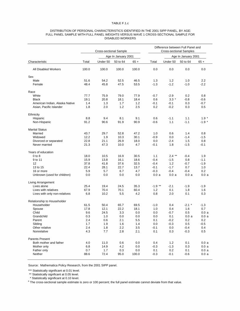
TABLE F.1.c

DISTRIBUTION OF PERSONAL CHARACTERISTICS IDENTIFIED IN THE 2001 SIPP PANEL, BY AGE:FULL PANEL SAMPLE WITH FULL PANEL WEIGHTS VERSUS WAVE 1 CROSS-SECTIONAL SAMPLE FOR

DISABLED WORKERS

Difference between Full Panel and Cross-sectional Sample Cross-sectional Samples

Age In January 2001 Age In January 2001

Characteristic Total Under 50 50 to 64 65 + Total Under 50 50 to 64 65 +

All Disabled Workers 100.0 100.0 100.0 100.0 0.0 0.0 0.0 0.0

SexMale 51.6 54.2 52.5 46.5 1.3 1.2 1.0 2.2 Female 48.4 45.8 47.5 53.5 -1.3 -1.2 -1.0 -2.2

RaceWhite 77.7 75.9 79.0 77.9 -0.7 -2.9 0.2 0.8 Black 19.1 20.8 18.1 18.4 0.6 3.3 * -0.8 -0.6 American Indian, Alaska Native 1.4 1.3 1.7 1.2 -0.1 -0.1 0.3 -0.7 Asian, Pacific Islander 1.8 2.0 1.2 2.5 0.2 -0.2 0.3 0.5

EthnicityHispanic 8.8 9.4 8.1 9.1 0.6 -1.1 1.1 1.9 *Non-Hispanic 91.2 90.6 91.9 90.9 -0.6 1.1 -1.1 -1.9 *

Marital StatusMarried 43.7 29.7 52.8 47.2 1.0 0.6 1.4 0.8 Widowed 12.2 1.9 10.3 30.1 -0.9 0.0 -1.4 -1.5 Divorced or separated 22.8 21.1 26.9 18.0 0.0 -2.4 1.5 0.8 Never married 21.3 47.3 10.0 4.7 -0.1 1.8 -1.5 -0.1

Years of education0 to 8 18.0 10.5 16.9 30.5 1.1 2.4 ** -0.4 1.9 9 to 11 15.9 13.8 16.1 18.6 -0.4 -1.5 0.8 -1.1 12 37.8 41.8 37.6 32.5 -0.4 1.2 -0.7 -1.9 13 to 15 22.4 28.1 22.7 13.7 -0.1 -1.7 0.7 1.0 16 or more 5.9 5.7 6.7 4.7 -0.3 -0.4 -0.4 0.2 Unknown (used for children) 0.0 0.0 0.0 0.0 0.0 a 0.0 a 0.0 a 0.0 a

Living ArrangementLives alone 25.4 19.4 24.5 35.3 -1.9 ** -2.1 -1.9 -1.9 Lives with relatives 67.9 70.4 70.1 60.4 1.2 0.1 1.8 1.6 Lives with only non-relatives 6.8 10.2 5.5 4.2 0.8 2.0 0.1 0.3

Relationship to HouseholderHouseholder 61.5 50.4 65.7 69.5 -1.0 0.4 -2.1 * -1.3 Spouse 17.8 12.1 22.2 18.1 1.0 0.4 1.6 0.7 Child 9.6 24.5 3.3 0.0 0.0 -0.7 0.5 0.0 aGrandchild 0.3 1.0 0.0 0.0 0.0 0.1 0.0 a 0.0 aParent 2.4 0.6 2.1 5.5 0.1 -0.2 0.2 0.2 Sibling 1.7 1.9 1.6 1.4 0.0 -0.3 0.5 -0.5 Other relative 2.4 1.8 2.2 3.5 -0.1 0.0 -0.4 0.4 Nonrelative 4.3 7.7 2.8 2.1 0.1 0.3 -0.3 0.5

Parents PresentBoth mother and father 4.0 11.0 0.6 0.0 0.4 1.2 0.1 0.0 aMother only 6.8 14.9 4.2 0.0 -0.3 -1.3 0.3 0.0 aFather only 0.7 1.7 0.3 0.0 0.1 0.2 0.1 0.0 aNeither 88.6 72.4 95.0 100.0 -0.3 -0.1 -0.6 0.0 a

Source: Mathematica Policy Research, from the 2001 SIPP panel.

*** Statistically significant at 0.01 level. ** Statistically signficant at 0.05 level. * Statistically significant at 0.10 level.a The cross-sectional sample estimate is zero or 100 percent; the full panel estimate cannot deviate from that value.

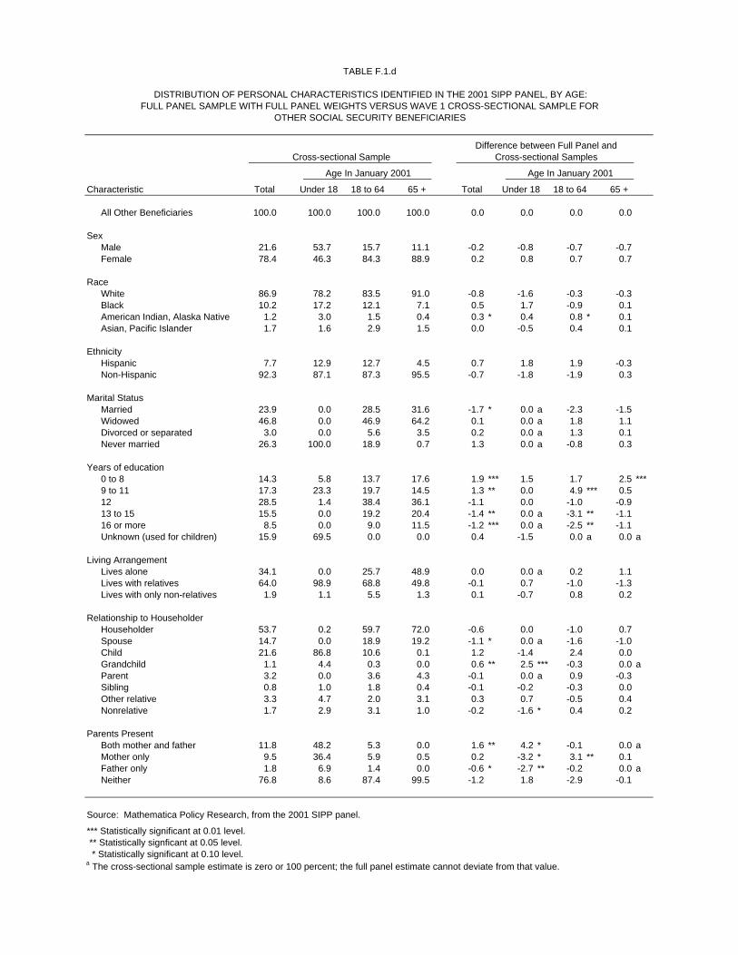
TABLE F.1.d

DISTRIBUTION OF PERSONAL CHARACTERISTICS IDENTIFIED IN THE 2001 SIPP PANEL, BY AGE:FULL PANEL SAMPLE WITH FULL PANEL WEIGHTS VERSUS WAVE 1 CROSS-SECTIONAL SAMPLE FOR

OTHER SOCIAL SECURITY BENEFICIARIES

Difference between Full Panel and Cross-sectional Sample Cross-sectional Samples

Age In January 2001 Age In January 2001

Characteristic Total Under 18 18 to 64 65 + Total Under 18 18 to 64 65 +

All Other Beneficiaries 100.0 100.0 100.0 100.0 0.0 0.0 0.0 0.0

SexMale 21.6 53.7 15.7 11.1 -0.2 -0.8 -0.7 -0.7 Female 78.4 46.3 84.3 88.9 0.2 0.8 0.7 0.7

RaceWhite 86.9 78.2 83.5 91.0 -0.8 -1.6 -0.3 -0.3 Black 10.2 17.2 12.1 7.1 0.5 1.7 -0.9 0.1 American Indian, Alaska Native 1.2 3.0 1.5 0.4 0.3 * 0.4 0.8 * 0.1 Asian, Pacific Islander 1.7 1.6 2.9 1.5 0.0 -0.5 0.4 0.1

EthnicityHispanic 7.7 12.9 12.7 4.5 0.7 1.8 1.9 -0.3 Non-Hispanic 92.3 87.1 87.3 95.5 -0.7 -1.8 -1.9 0.3

Marital StatusMarried 23.9 0.0 28.5 31.6 -1.7 * 0.0 a -2.3 -1.5 Widowed 46.8 0.0 46.9 64.2 0.1 0.0 a 1.8 1.1 Divorced or separated 3.0 0.0 5.6 3.5 0.2 0.0 a 1.3 0.1 Never married 26.3 100.0 18.9 0.7 1.3 0.0 a -0.8 0.3

Years of education0 to 8 14.3 5.8 13.7 17.6 1.9 *** 1.5 1.7 2.5 ***9 to 11 17.3 23.3 19.7 14.5 1.3 ** 0.0 4.9 *** 0.5 12 28.5 1.4 38.4 36.1 -1.1 0.0 -1.0 -0.9 13 to 15 15.5 0.0 19.2 20.4 -1.4 ** 0.0 a -3.1 ** -1.1 16 or more 8.5 0.0 9.0 11.5 -1.2 *** 0.0 a -2.5 ** -1.1 Unknown (used for children) 15.9 69.5 0.0 0.0 0.4 -1.5 0.0 a 0.0 a

Living ArrangementLives alone 34.1 0.0 25.7 48.9 0.0 0.0 a 0.2 1.1 Lives with relatives 64.0 98.9 68.8 49.8 -0.1 0.7 -1.0 -1.3 Lives with only non-relatives 1.9 1.1 5.5 1.3 0.1 -0.7 0.8 0.2

Relationship to HouseholderHouseholder 53.7 0.2 59.7 72.0 -0.6 0.0 -1.0 0.7 Spouse 14.7 0.0 18.9 19.2 -1.1 * 0.0 a -1.6 -1.0 Child 21.6 86.8 10.6 0.1 1.2 -1.4 2.4 0.0 Grandchild 1.1 4.4 0.3 0.0 0.6 ** 2.5 *** -0.3 0.0 aParent 3.2 0.0 3.6 4.3 -0.1 0.0 a 0.9 -0.3 Sibling 0.8 1.0 1.8 0.4 -0.1 -0.2 -0.3 0.0 Other relative 3.3 4.7 2.0 3.1 0.3 0.7 -0.5 0.4 Nonrelative 1.7 2.9 3.1 1.0 -0.2 -1.6 * 0.4 0.2

Parents PresentBoth mother and father 11.8 48.2 5.3 0.0 1.6 ** 4.2 * -0.1 0.0 aMother only 9.5 36.4 5.9 0.5 0.2 -3.2 * 3.1 ** 0.1 Father only 1.8 6.9 1.4 0.0 -0.6 * -2.7 ** -0.2 0.0 aNeither 76.8 8.6 87.4 99.5 -1.2 1.8 -2.9 -0.1

Source: Mathematica Policy Research, from the 2001 SIPP panel.

*** Statistically significant at 0.01 level. ** Statistically signficant at 0.05 level. * Statistically significant at 0.10 level.a The cross-sectional sample estimate is zero or 100 percent; the full panel estimate cannot deviate from that value.

TABLE F.1.e

DISTRIBUTION OF PERSONAL CHARACTERISTICS IDENTIFIED IN THE 2001 SIPP PANEL, BY AGE:FULL PANEL SAMPLE WITH FULL PANEL WEIGHTS VERSUS WAVE 1 CROSS-SECTIONAL SAMPLE FOR

SSI RECIPIENTS

Difference between Full Panel and Cross-sectional Sample Cross-sectional Samples

Age In January 2001 Age In January 2001

Characteristic Total Under 18 18 to 64 65 + Total Under 18 18 to 64 65 +

All SSI Recipients 100.0 100.0 100.0 100.0 0.0 0.0 0.0 0.0

SexMale 43.8 62.1 46.6 25.6 0.4 2.0 0.4 1.3 Female 56.2 37.9 53.4 74.4 -0.4 -2.0 -0.4 -1.3

RaceWhite 62.6 57.4 65.5 57.4 -0.3 -0.8 -1.1 1.3 Black 29.7 39.0 29.1 26.1 -0.3 -1.4 0.3 -0.4 American Indian, Alaska Native 2.2 3.2 2.4 1.2 0.9 *** 1.7 1.0 *** 0.3 Asian, Pacific Islander 5.5 0.5 3.0 15.3 -0.3 0.6 -0.2 -1.2

EthnicityHispanic 16.1 18.4 13.9 21.0 0.0 -2.1 -0.7 3.5 *Non-Hispanic 83.9 81.6 86.1 79.0 0.0 2.1 0.7 -3.5 *

Marital StatusMarried 21.6 0.3 23.4 28.7 0.7 0.7 0.2 -0.6 Widowed 13.9 0.0 6.1 43.1 0.5 0.0 a 0.0 1.0 Divorced or separated 22.9 0.0 28.8 19.3 -0.9 0.0 a -1.7 -1.8 Never married 41.6 99.7 41.7 8.9 -0.3 -0.7 1.5 1.4

Years of education0 to 8 25.1 8.1 19.7 49.7 2.4 *** 4.9 ** 0.7 4.5 **9 to 11 21.0 18.2 23.1 16.6 -0.6 2.7 -0.7 -2.2 12 28.7 1.2 36.7 21.9 0.8 -0.2 0.7 -1.7 13 to 15 12.6 0.0 16.9 7.6 -0.3 0.0 a -1.0 -0.1 16 or more 3.3 0.0 3.7 4.1 0.1 0.0 a 0.2 -0.5 Unknown (used for children) 9.4 72.6 0.0 0.0 -2.5 *** -7.4 * 0.0 a 0.0 a

Living ArrangementLives alone 25.6 0.0 24.3 43.5 1.0 0.0 a 0.3 0.7 Lives with relatives 66.2 96.9 64.1 54.9 -0.8 1.3 0.1 -0.8 Lives with only non-relatives 8.2 3.1 11.6 1.6 -0.1 -1.3 -0.3 0.2

Relationship to HouseholderHouseholder 50.3 0.5 54.0 68.2 1.7 0.7 0.3 0.3 Spouse 8.8 0.0 9.9 10.8 0.0 0.0 a -0.1 -0.8 Child 23.1 81.5 19.5 0.3 -1.0 -0.2 0.9 0.1 Grandchild 1.7 10.4 0.5 0.0 0.2 4.0 0.1 0.0 aParent 3.8 0.0 2.0 11.0 -0.2 0.0 a -0.1 -1.1 Sibling 3.0 0.3 3.8 2.4 -0.4 -0.3 -0.4 -0.8 Other relative 3.7 3.4 2.7 6.5 -0.2 -2.8 ** -0.6 2.3 *Nonrelative 5.6 3.8 7.7 0.8 -0.1 -1.4 0.0 0.0

Parents PresentBoth mother and father 11.2 35.7 10.3 0.0 0.7 6.0 1.0 0.0 aMother only 13.4 46.7 11.3 0.5 -1.7 * -9.7 ** 0.3 -0.1 Father only 1.6 4.0 1.6 0.0 0.6 * 2.7 ** 0.5 0.0 aNeither 73.9 13.6 76.8 99.5 0.5 1.0 -1.9 0.1

Source: Mathematica Policy Research, from the 2001 SIPP panel.

*** Statistically significant at 0.01 level. ** Statistically signficant at 0.05 level. * Statistically significant at 0.10 level.a The cross-sectional sample estimate is zero or 100 percent; the full panel estimate cannot deviate from that value.

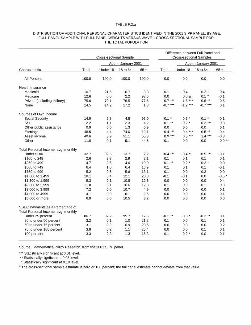
TABLE F.2.a

DISTRIBUTION OF ADDITIONAL PERSONAL CHARACTERISTICS IDENTIFIED IN THE 2001 SIPP PANEL, BY AGE:FULL PANEL SAMPLE WITH FULL PANEL WEIGHTS VERSUS WAVE 1 CROSS-SECTIONAL SAMPLE FOR

THE TOTAL POPULATION

Difference between Full Panel and Cross-sectional Sample Cross-sectional Samples

Age In January 2001 Age In January 2001

Characteristic Total Under 18 18 to 64 65 + Total Under 18 18 to 64 65 +

All Persons 100.0 100.0 100.0 100.0 0.0 0.0 0.0 0.0

Health InsuranceMedicaid 10.7 21.6 6.7 8.3 0.1 -0.4 0.2 * 0.4 Medicare 12.6 0.0 2.2 93.6 0.0 0.0 a 0.1 * -0.1 Private (including military) 75.0 70.1 76.5 77.5 0.7 *** 1.5 *** 0.6 ** -0.5 None 14.5 14.2 17.2 1.3 -0.7 *** -1.2 *** -0.7 *** 0.1

Sources of Own IncomeSocial Security 14.9 2.8 4.8 93.0 0.1 * 0.3 * 0.1 * -0.1 SSI 2.2 1.1 2.3 4.2 0.1 ** -0.2 * 0.2 *** 0.3 Other public assistance 0.9 0.0 1.3 0.9 0.0 0.0 0.0 0.1 Earnings 48.5 4.4 74.0 12.1 0.4 *** 0.4 *** 0.5 ** 0.4 Asset income 40.6 3.9 51.1 65.8 0.9 *** 0.5 *** 1.4 *** -0.8 Other 11.0 0.1 9.1 44.3 0.1 0.0 0.0 0.9 **

Total Personal Income, avg. monthlyUnder $100 32.7 92.5 13.7 2.2 -0.4 *** -0.4 ** -0.5 *** -0.1 $100 to 249 2.6 2.3 2.9 2.1 0.1 0.1 0.1 0.1 $250 to 499 4.7 2.5 4.6 10.0 0.1 ** 0.2 * 0.2 * 0.0 $500 to 749 6.4 1.6 6.4 16.9 0.1 0.1 0.1 -0.1 $750 to 999 5.2 0.5 5.6 13.1 0.1 0.0 0.2 0.0 $1,000 to 1,499 10.1 0.4 12.1 20.3 -0.1 -0.1 0.0 -0.5 *$1,500 to 1,999 8.3 0.1 10.8 12.5 0.0 0.0 0.0 0.4 $2,000 to 2,999 11.8 0.1 16.6 12.3 0.1 0.0 0.1 0.3 $3,000 to 3,999 7.2 0.0 10.7 4.9 0.0 0.0 0.0 0.1 $4,000 to 4999 4.1 0.0 6.1 2.5 0.0 0.0 0.0 -0.1 $5,000 or more 6.9 0.0 10.5 3.2 0.0 0.0 0.0 0.0

SSEC Payments as a Percentage ofTotal Personal Income, avg. monthly

Under 25 percent 86.7 97.2 95.7 17.5 -0.1 ** -0.3 * -0.2 ** 0.1 25 to under 50 percent 3.2 0.1 1.0 21.2 0.1 0.0 0.1 0.1 50 to under 75 percent 3.1 0.2 0.9 20.6 0.0 0.0 0.0 -0.2 75 to under 100 percent 3.8 0.2 1.1 25.4 0.0 0.0 0.1 0.1 100 percent 3.3 2.3 1.3 15.3 0.1 0.2 * 0.0 -0.1

Source: Mathematica Policy Research, from the 2001 SIPP panel.

*** Statistically significant at 0.01 level. ** Statistically signficant at 0.05 level. * Statistically significant at 0.10 level.a The cross-sectional sample estimate is zero or 100 percent; the full panel estimate cannot deviate from that value.

TABLE F.2.b

DISTRIBUTION OF ADDITIONAL PERSONAL CHARACTERISTICS IDENTIFIED IN THE 2001 SIPP PANEL, BY AGE:FULL PANEL SAMPLE WITH FULL PANEL WEIGHTS VERSUS WAVE 1 CROSS-SECTIONAL SAMPLE FOR

RETIRED WORKERS

Difference between Full Panel and Cross-sectional Sample Cross-sectional Samples

Age In January 2001 Age In January 2001

Characteristic Total Under 65 65 to 74 75 + Total Under 65 65 to 74 75 +

All Retired Workers 100.0 100.0 100.0 100.0 0.0 0.0 0.0 0.0

Health InsuranceMedicaid 5.8 5.7 5.8 5.9 0.3 0.6 0.0 0.4 Medicare 91.5 19.4 99.9 100.0 -0.1 -1.7 0.0 * 0.0 aPrivate (including military) 80.4 80.1 81.0 79.7 -0.5 -3.7 *** -0.4 0.2 None 1.0 9.6 0.0 0.0 0.3 *** 2.6 *** 0.0 0.0 a

Sources of Own IncomeSocial Security 100.0 100.0 100.0 100.0 0.0 a 0.0 a 0.0 a 0.0 aSSI 2.3 2.4 2.3 2.1 0.1 0.6 -0.1 0.3 *Other public assistance 0.6 0.3 0.6 0.7 0.0 -0.2 0.0 0.1 Earnings 12.6 21.6 17.1 5.0 0.5 ** 2.5 ** 0.8 * -0.2 Asset income 68.5 62.5 68.6 69.8 -0.6 -0.2 -0.7 -0.5 Other 47.2 43.7 46.1 49.3 0.8 * -2.3 ** 1.3 ** 1.1

Total Personal Income, avg. monthlyUnder $100 0.4 0.6 0.5 0.3 0.1 0.3 ** 0.0 0.1 $100 to 249 1.8 2.2 1.9 1.6 0.0 -0.2 0.0 0.1 $250 to 499 9.7 10.8 10.3 8.8 -0.2 -0.9 0.0 -0.2 $500 to 749 15.4 13.8 14.1 17.3 -0.2 0.4 -0.2 -0.3 $750 to 999 13.2 11.9 12.2 14.6 0.2 1.2 -0.4 0.5 $1,000 to 1,499 21.0 16.6 20.1 23.2 -0.5 1.4 -0.4 -1.0 *$1,500 to 1,999 13.5 12.1 13.4 14.0 0.3 -0.4 0.1 0.6 $2,000 to 2,999 13.6 16.2 14.7 11.7 0.3 -1.5 0.6 0.4 $3,000 to 3,999 5.5 8.9 5.8 4.4 0.2 0.5 0.2 0.1 $4,000 to 4999 2.8 4.1 3.3 1.9 -0.2 -0.4 -0.1 -0.3 *$5,000 or more 3.0 2.9 3.8 2.1 0.0 -0.3 0.1 0.1

SSEC Payments as a Percentage ofTotal Personal Income, avg. monthly

Under 25 percent 11.6 16.0 13.4 8.4 -0.2 -1.6 0.3 -0.3 25 to under 50 percent 24.3 28.5 25.1 22.4 0.3 1.2 0.4 0.0 50 to under 75 percent 22.4 18.5 22.5 23.1 0.0 0.9 -0.5 0.3 75 to under 100 percent 26.5 19.8 24.8 30.2 0.1 0.3 0.0 0.2 100 percent 15.2 17.2 14.2 15.9 -0.2 -0.9 -0.2 -0.1

Source: Mathematica Policy Research, from the 2001 SIPP panel.

*** Statistically significant at 0.01 level. ** Statistically signficant at 0.05 level. * Statistically significant at 0.10 level.a The cross-sectional sample estimate is zero or 100 percent; the full panel estimate cannot deviate from that value.

TABLE F.2.c

DISTRIBUTION OF ADDITIONAL PERSONAL CHARACTERISTICS IDENTIFIED IN THE 2001 SIPP PANEL, BY AGE:FULL PANEL SAMPLE WITH FULL PANEL WEIGHTS VERSUS WAVE 1 CROSS-SECTIONAL SAMPLE FOR

DISABLED WORKERS

Difference between Full Panel and Cross-sectional Sample Cross-sectional Samples

Age In January 2001 Age In January 2001

Characteristic Total Under 50 50 to 64 65 + Total Under 50 50 to 64 65 +

All Disabled Workers 100.0 100.0 100.0 100.0 0.0 0.0 0.0 0.0

Health InsuranceMedicaid 35.8 50.2 28.1 29.2 0.4 -0.3 0.2 1.6 Medicare 78.1 70.8 71.6 100.0 0.8 1.4 0.7 0.0 aPrivate (including military) 41.9 31.4 44.9 51.4 0.5 1.5 -0.6 1.3 None 3.2 4.2 4.3 0.0 -0.4 -0.7 -0.5 0.0 a

Sources of Own IncomeSocial Security 100.0 100.0 100.0 100.0 0.0 a 0.0 a 0.0 a 0.0 aSSI 19.2 27.9 15.1 14.5 -0.3 -0.5 0.4 -1.0 Other public assistance 3.6 4.9 3.1 2.6 -0.1 0.3 -0.6 0.1 Earnings 8.0 15.0 4.7 3.9 1.3 ** 2.1 0.2 2.2 ***Asset income 30.0 22.3 32.8 35.9 0.8 0.9 -0.2 2.4 Other 25.0 15.6 29.8 29.8 0.6 1.2 -1.4 3.2 **

Total Personal Income, avg. monthlyUnder $100 0.5 0.5 0.4 0.5 0.1 -0.2 0.2 0.2 $100 to 249 1.9 1.8 1.8 2.1 0.6 ** 0.5 0.8 *** 0.3 $250 to 499 9.3 8.0 7.7 14.0 0.1 1.3 0.6 -2.3 *$500 to 749 33.1 41.1 28.3 30.6 -1.8 * -2.5 -1.0 -2.1 $750 to 999 19.0 18.5 20.4 17.1 0.2 -0.2 0.6 -0.1 $1,000 to 1,499 19.6 17.2 22.0 18.5 0.3 0.2 -0.3 1.5 $1,500 to 1,999 6.5 6.3 6.5 6.8 0.0 -0.1 -0.7 1.5 *$2,000 to 2,999 6.7 4.5 7.8 8.1 0.2 0.9 -0.5 0.3 $3,000 to 3,999 2.3 1.2 3.6 1.5 0.3 0.2 0.4 0.4 $4,000 to 4999 0.5 0.2 0.8 0.4 0.1 -0.1 0.1 0.2 $5,000 or more 0.6 0.6 0.8 0.4 -0.1 -0.1 -0.2 0.0

SSEC Payments as a Percentage ofTotal Personal Income, avg. monthly

Under 25 percent 5.4 7.7 4.5 3.6 0.3 0.9 -0.5 0.6 25 to under 50 percent 13.9 14.1 13.8 13.7 0.5 1.6 -0.9 1.5 50 to under 75 percent 19.3 19.4 17.6 22.0 0.0 -0.6 0.1 0.8 75 to under 100 percent 25.1 23.7 26.0 25.6 0.3 -0.3 0.6 0.4 100 percent 36.3 35.1 38.0 35.1 -1.1 -1.6 0.6 -3.3 *

Source: Mathematica Policy Research, from the 2001 SIPP panel.

*** Statistically significant at 0.01 level. ** Statistically signficant at 0.05 level. * Statistically significant at 0.10 level.a The cross-sectional sample estimate is zero or 100 percent; the full panel estimate cannot deviate from that value.

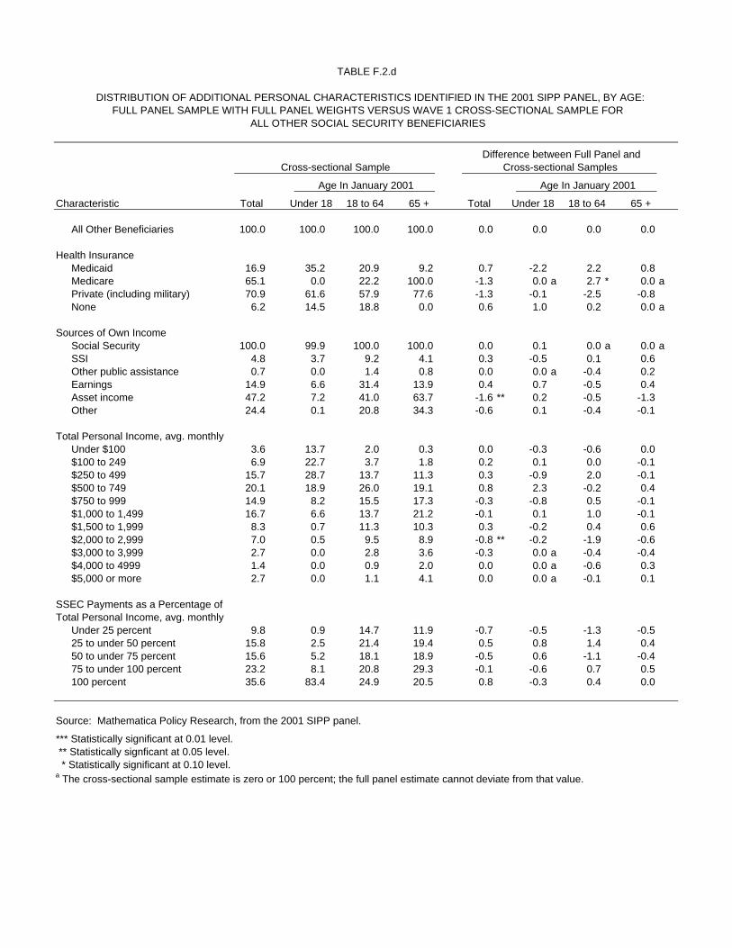
TABLE F.2.d

DISTRIBUTION OF ADDITIONAL PERSONAL CHARACTERISTICS IDENTIFIED IN THE 2001 SIPP PANEL, BY AGE:FULL PANEL SAMPLE WITH FULL PANEL WEIGHTS VERSUS WAVE 1 CROSS-SECTIONAL SAMPLE FOR

ALL OTHER SOCIAL SECURITY BENEFICIARIES

Difference between Full Panel and Cross-sectional Sample Cross-sectional Samples

Age In January 2001 Age In January 2001

Characteristic Total Under 18 18 to 64 65 + Total Under 18 18 to 64 65 +

All Other Beneficiaries 100.0 100.0 100.0 100.0 0.0 0.0 0.0 0.0

Health InsuranceMedicaid 16.9 35.2 20.9 9.2 0.7 -2.2 2.2 0.8 Medicare 65.1 0.0 22.2 100.0 -1.3 0.0 a 2.7 * 0.0 aPrivate (including military) 70.9 61.6 57.9 77.6 -1.3 -0.1 -2.5 -0.8 None 6.2 14.5 18.8 0.0 0.6 1.0 0.2 0.0 a

Sources of Own IncomeSocial Security 100.0 99.9 100.0 100.0 0.0 0.1 0.0 a 0.0 aSSI 4.8 3.7 9.2 4.1 0.3 -0.5 0.1 0.6 Other public assistance 0.7 0.0 1.4 0.8 0.0 0.0 a -0.4 0.2 Earnings 14.9 6.6 31.4 13.9 0.4 0.7 -0.5 0.4 Asset income 47.2 7.2 41.0 63.7 -1.6 ** 0.2 -0.5 -1.3 Other 24.4 0.1 20.8 34.3 -0.6 0.1 -0.4 -0.1

Total Personal Income, avg. monthlyUnder $100 3.6 13.7 2.0 0.3 0.0 -0.3 -0.6 0.0 $100 to 249 6.9 22.7 3.7 1.8 0.2 0.1 0.0 -0.1 $250 to 499 15.7 28.7 13.7 11.3 0.3 -0.9 2.0 -0.1 $500 to 749 20.1 18.9 26.0 19.1 0.8 2.3 -0.2 0.4 $750 to 999 14.9 8.2 15.5 17.3 -0.3 -0.8 0.5 -0.1 $1,000 to 1,499 16.7 6.6 13.7 21.2 -0.1 0.1 1.0 -0.1 $1,500 to 1,999 8.3 0.7 11.3 10.3 0.3 -0.2 0.4 0.6 $2,000 to 2,999 7.0 0.5 9.5 8.9 -0.8 ** -0.2 -1.9 -0.6 $3,000 to 3,999 2.7 0.0 2.8 3.6 -0.3 0.0 a -0.4 -0.4 $4,000 to 4999 1.4 0.0 0.9 2.0 0.0 0.0 a -0.6 0.3 $5,000 or more 2.7 0.0 1.1 4.1 0.0 0.0 a -0.1 0.1

SSEC Payments as a Percentage ofTotal Personal Income, avg. monthly

Under 25 percent 9.8 0.9 14.7 11.9 -0.7 -0.5 -1.3 -0.5 25 to under 50 percent 15.8 2.5 21.4 19.4 0.5 0.8 1.4 0.4 50 to under 75 percent 15.6 5.2 18.1 18.9 -0.5 0.6 -1.1 -0.4 75 to under 100 percent 23.2 8.1 20.8 29.3 -0.1 -0.6 0.7 0.5 100 percent 35.6 83.4 24.9 20.5 0.8 -0.3 0.4 0.0

Source: Mathematica Policy Research, from the 2001 SIPP panel.

*** Statistically significant at 0.01 level. ** Statistically signficant at 0.05 level. * Statistically significant at 0.10 level.a The cross-sectional sample estimate is zero or 100 percent; the full panel estimate cannot deviate from that value.

TABLE F.2.e

DISTRIBUTION OF ADDITIONAL PERSONAL CHARACTERISTICS IDENTIFIED IN THE 2001 SIPP PANEL, BY AGE:FULL PANEL SAMPLE WITH FULL PANEL WEIGHTS VERSUS WAVE 1 CROSS-SECTIONAL SAMPLE FOR

SSI RECIPIENTS

Difference between Full Panel and Cross-sectional Sample Cross-sectional Samples

Age In January 2001 Age In January 2001

Characteristic Total Under 18 18 to 64 65 + Total Under 18 18 to 64 65 +

All SSI Recipients 100.0 100.0 100.0 100.0 0.0 0.0 0.0 0.0

Health InsuranceMedicaid 93.3 81.1 94.2 97.7 0.9 1.2 0.6 0.1 Medicare 26.3 0.0 18.6 62.6 0.5 0.0 a 0.6 -2.2 Private (including military) 16.9 35.7 15.4 10.3 0.6 9.8 ** 0.3 -0.7 None 2.9 7.4 2.9 0.4 -0.5 -3.4 * -0.1 0.3

Sources of Own IncomeSocial Security 32.1 9.3 25.7 62.6 -0.5 1.2 -0.9 -2.2 SSI 100.0 100.0 100.0 100.0 0.0 a 0.0 a 0.0 a 0.0 aOther public assistance 8.2 0.6 10.7 5.5 0.2 0.3 -0.6 1.4 *Earnings 7.4 5.2 10.1 1.2 1.1 * 1.2 1.3 0.2 Asset income 10.8 3.5 11.6 12.6 0.7 2.9 0.7 -1.2 Other 7.5 0.0 8.5 9.1 0.4 0.0 a 0.0 0.9

Total Personal Income, avg. monthlyUnder $100 1.9 8.4 1.1 0.2 -0.5 -3.2 -0.1 0.1 $100 to 249 4.3 18.8 2.4 1.6 -0.9 * -3.3 -0.3 0.1 $250 to 499 15.2 26.8 11.4 19.4 0.0 1.5 0.1 0.6 $500 to 749 56.5 36.1 58.7 61.6 1.6 4.0 0.8 0.5 $750 to 999 8.4 2.8 10.0 7.3 1.1 ** 0.4 1.4 ** -0.1 $1,000 to 1,499 8.5 5.0 9.9 6.6 -0.7 2.2 -1.1 -1.1 $1,500 to 1,999 2.5 1.4 3.2 1.2 -0.5 * -0.9 -0.7 * -0.1 $2,000 to 2,999 1.7 0.8 2.0 1.5 0.0 -0.8 0.1 0.0 $3,000 to 3,999 0.7 0.0 1.0 0.3 0.0 0.0 a 0.0 0.1 $4,000 to 4999 0.2 0.0 0.2 0.2 -0.1 0.0 a -0.1 -0.2 $5,000 or more 0.1 0.0 0.1 0.2 -0.1 0.0 a -0.1 0.0

SSEC Payments as a Percentage ofTotal Personal Income, avg. monthly

Under 25 percent 70.9 91.6 77.4 41.2 0.2 -1.4 0.9 0.7 25 to under 50 percent 6.4 1.3 5.7 10.9 0.3 0.5 0.6 -1.1 50 to under 75 percent 12.5 5.2 9.4 25.3 -0.3 1.2 -0.5 -1.0 75 to under 100 percent 10.2 1.9 7.4 22.6 -0.2 -0.3 -1.0 1.4 100 percent 0.0 0.0 0.0 0.0 0.0 a 0.0 a 0.0 a 0.0 a

Source: Mathematica Policy Research, from the 2001 SIPP panel.

*** Statistically significant at 0.01 level. ** Statistically signficant at 0.05 level. * Statistically significant at 0.10 level.a The cross-sectional sample estimate is zero or 100 percent; the full panel estimate cannot deviate from that value.

TABLE F.3.a

DISTRIBUTION OF HOUSEHOLD AND FAMILY CHARACTERISTICS IDENTIFIED IN THE 2001 SIPP PANEL, BY AGE:FULL PANEL SAMPLE WITH FULL PANEL WEIGHTS VERSUS WAVE 1 CROSS-SECTIONAL SAMPLE FOR

THE TOTAL POPULATION

Difference between Full Panel and Cross-sectional Sample Cross-sectional Samples

Age In January 2001 Age In January 2001

Characteristic Total Under 18 18 to 64 65 + Total Under 18 18 to 64 65 +

All Persons 100.0 100.0 100.0 100.0 0.0 0.0 0.0 0.0

Household TypeFamily Married couple present 64.5 70.0 63.6 57.7 1.4 *** 2.0 *** 1.6 *** -0.7 No married couple present Male householder 5.1 5.6 5.3 2.9 -0.4 ** -0.4 * -0.5 *** 0.1 Female householder 15.1 23.4 13.1 7.3 -0.7 *** -1.4 ** -0.5 *** -0.1 Nonfamily Male householder 7.2 0.8 9.9 7.7 -0.3 *** -0.2 ** -0.5 *** 0.4 Female householder 7.8 0.2 7.9 24.0 0.0 0.0 0.0 0.3

Ownership Status of Living QuartersOwned 70.1 66.8 69.0 83.0 1.6 *** 2.2 *** 1.6 *** 0.6 Not owned 29.9 33.2 31.0 17.0 -1.6 *** -2.2 *** -1.6 *** -0.6

Residence in Public Housing 2.4 3.4 1.8 2.9 0.0 -0.1 0.0 0.0

Household Size1 person 10.1 0.0 10.4 30.3 -0.1 0.0 -0.1 0.3 2 persons 26.8 4.6 30.5 55.3 -0.5 -0.3 -0.6 -0.3 3 to 4 persons 41.5 53.6 42.3 11.3 0.2 -0.1 0.4 -0.2 5 or more persons 21.6 41.7 16.8 3.1 0.3 0.3 0.4 0.1

Family Size1 person 16.5 0.9 20.0 32.1 -0.6 *** -0.3 *** -1.0 *** 0.7 2 persons 24.7 6.4 26.6 54.3 -0.7 -0.8 -0.7 -0.7 3 to 4 persons 39.0 53.5 38.5 10.7 0.8 0.2 1.1 -0.1 5 or more persons 19.8 39.1 14.9 2.9 0.6 0.8 0.6 0.1

Persons under 18 in FamilyNone 46.5 1.0 56.2 94.9 -1.0 -0.2 *** -1.5 0.0 1 person 17.6 22.3 18.5 2.6 -0.1 -0.8 0.2 0.0 2 persons 20.1 38.6 15.9 1.6 0.9 1.1 ** 1.0 0.1 3 persons 10.3 23.7 6.5 0.6 0.1 0.0 0.2 0.0 4 persons 3.5 8.9 1.9 0.2 0.1 0.1 0.1 0.0 5 or more persons 2.0 5.4 0.9 0.1 0.0 -0.1 0.0 0.0

Source: Mathematica Policy Research, from the 2001 SIPP panel.

*** Statistically significant at 0.01 level. ** Statistically signficant at 0.05 level. * Statistically significant at 0.10 level.a The cross-sectional sample estimate is zero or 100 percent; the full panel estimate cannot deviate from that value.

TABLE F.3.b

DISTRIBUTION OF HOUSEHOLD AND FAMILY CHARACTERISTICS IDENTIFIED IN THE 2001 SIPP PANEL, BY AGE:FULL PANEL SAMPLE WITH FULL PANEL WEIGHTS VERSUS WAVE 1 CROSS-SECTIONAL SAMPLE FOR

RETIRED WORKERS

Difference between Full Panel and Cross-sectional Sample Cross-sectional Samples

Age In January 2001 Age In January 2001

Characteristic Total Under 65 65 to 74 75 + Total Under 65 65 to 74 75 +

All Retired Workers 100.0 100.0 100.0 100.0 0.0 0.0 0.0 0.0

Household TypeFamily Married couple present 62.2 74.7 69.4 50.6 -1.0 -1.3 -1.0 -0.8 No married couple present Male householder 2.6 2.5 2.2 3.2 0.1 -0.6 0.2 0.2 Female householder 6.0 6.0 5.0 7.2 0.1 1.1 * -0.3 0.4 Nonfamily Male householder 8.6 8.1 7.7 9.6 0.4 0.2 0.8 -0.1 Female householder 20.3 8.5 15.6 28.8 0.4 0.5 0.3 0.3

Ownership Status of Living QuartersOwned 85.1 87.2 87.6 81.7 0.6 0.0 -0.1 1.5 *Not owned 14.9 12.8 12.4 18.3 -0.6 0.0 0.1 -1.5 *

Residence in Public Housing 2.2 1.2 1.6 3.0 -0.1 0.4 -0.2 -0.1

Household Size1 person 27.2 13.1 21.6 37.3 0.3 0.3 0.5 -0.1 2 persons 58.8 65.0 63.8 51.4 -0.5 -0.9 0.0 -0.9 3 to 4 persons 11.3 17.5 11.8 9.2 0.1 1.1 -0.6 0.7 5 or more persons 2.7 4.4 2.8 2.1 0.1 -0.4 0.0 0.3

Family Size1 person 29.4 17.1 23.6 39.1 0.7 0.5 1.2 0.2 2 persons 57.5 63.0 62.5 50.4 -0.9 -1.2 -0.6 -1.2 3 to 4 persons 10.6 16.2 11.3 8.5 0.2 0.8 -0.5 0.8 5 or more persons 2.5 3.7 2.7 2.0 0.1 -0.1 -0.1 0.3

Persons under 18 in FamilyNone 95.5 92.3 94.7 97.1 -0.2 -1.0 0.1 -0.3 1 person 2.4 4.3 2.7 1.5 0.1 0.5 0.1 0.1 2 persons 1.3 2.2 1.7 0.8 0.1 0.1 0.1 0.2 *3 persons 0.5 0.9 0.6 0.4 -0.1 0.3 -0.2 0.0 4 persons 0.1 0.1 0.2 0.1 0.0 0.1 0.0 0.0 5 or more persons 0.1 0.2 0.2 0.0 0.0 0.0 0.0 0.0

Source: Mathematica Policy Research, from the 2001 SIPP panel.

*** Statistically significant at 0.01 level. ** Statistically signficant at 0.05 level. * Statistically significant at 0.10 level.a The cross-sectional sample estimate is zero or 100 percent; the full panel estimate cannot deviate from that value.

TABLE F.3.c

DISTRIBUTION OF HOUSEHOLD AND FAMILY CHARACTERISTICS IDENTIFIED IN THE 2001 SIPP PANEL, BY AGE:FULL PANEL SAMPLE WITH FULL PANEL WEIGHTS VERSUS WAVE 1 CROSS-SECTIONAL SAMPLE FOR

DISABLED WORKERS

Difference between Full Panel and Cross-sectional Sample Cross-sectional Samples

Age In January 2001 Age In January 2001

Characteristic Total Under 50 50 to 64 65 + Total Under 50 50 to 64 65 +

All Disabled Workers 100.0 100.0 100.0 100.0 0.0 0.0 0.0 0.0

Household TypeFamily Married couple present 48.2 41.2 53.7 48.2 1.4 2.1 1.0 1.3 No married couple present Male householder 4.0 4.9 3.5 3.7 0.2 0.8 -0.4 0.7 Female householder 16.8 26.1 13.8 8.9 -0.3 -2.0 0.9 0.0 Nonfamily Male householder 13.2 15.8 11.8 11.8 0.2 0.1 0.8 -0.6 Female householder 17.5 11.4 16.7 27.4 -1.8 ** -1.9 -2.0 * -1.4

Ownership Status of Living QuartersOwned 64.3 55.8 69.9 66.4 0.6 0.8 -0.6 2.3 Not owned 35.7 44.2 30.1 33.6 -0.6 -0.8 0.6 -2.3

Residence in Public Housing 6.5 6.0 5.3 9.3 0.0 0.2 0.1 -0.5

Household Size1 person 25.4 19.4 24.5 35.3 -1.9 ** -2.1 -1.9 -1.9 2 persons 41.6 31.6 47.1 45.8 1.3 -1.1 2.5 2.5 3 to 4 persons 24.8 36.9 21.2 14.2 0.1 0.1 0.7 -0.9 5 or more persons 8.3 12.2 7.2 4.6 0.5 3.1 ** -1.3 0.2

Family Size1 person 32.1 29.6 29.9 39.6 -1.2 -0.1 -1.8 -1.6 2 persons 38.1 27.7 43.9 42.5 0.9 -2.0 2.2 2.6 3 to 4 persons 22.6 31.7 20.4 13.5 0.0 0.1 0.5 -0.9 5 or more persons 7.2 11.0 5.8 4.4 0.3 2.0 -0.9 -0.1

Persons under 18 in FamilyNone 82.1 71.1 85.0 92.5 -0.5 -2.6 1.1 -0.5 1 person 9.0 12.9 8.6 4.3 -0.2 0.1 -0.7 0.2 2 persons 5.1 8.7 3.7 2.5 0.5 1.1 0.2 0.3 3 persons 2.3 4.6 1.4 0.4 0.2 0.9 -0.3 0.2 4 persons 0.9 1.6 0.7 0.2 -0.2 -0.2 -0.3 -0.2 5 or more persons 0.7 1.1 0.7 0.0 0.2 0.8 * -0.1 0.0 a

Source: Mathematica Policy Research, from the 2001 SIPP panel.

*** Statistically significant at 0.01 level. ** Statistically signficant at 0.05 level. * Statistically significant at 0.10 level.a The cross-sectional sample estimate is zero or 100 percent; the full panel estimate cannot deviate from that value.

TABLE F.3.d

DISTRIBUTION OF HOUSEHOLD AND FAMILY CHARACTERISTICS IDENTIFIED IN THE 2001 SIPP PANEL, BY AGE:FULL PANEL SAMPLE WITH FULL PANEL WEIGHTS VERSUS WAVE 1 CROSS-SECTIONAL SAMPLE FOR

ALL OTHER SOCIAL SECURITY BENEFICIARIES

Difference between Full Panel and Cross-sectional Sample Cross-sectional Samples

Age In January 2001 Age In January 2001

Characteristic Total Under 18 18 to 64 65 + Total Under 18 18 to 64 65 +

All Other Beneficiaries 100.0 100.0 100.0 100.0 0.0 0.0 0.0 0.0

Household TypeFamily Married couple present 38.1 50.3 36.5 34.0 0.3 5.2 ** -2.0 -1.4 No married couple present Male householder 4.2 9.3 4.7 2.1 -0.6 -2.7 ** 0.0 -0.1 Female householder 21.7 39.0 27.9 13.8 0.4 -1.9 1.9 0.2 Nonfamily Male householder 1.9 1.3 4.7 1.5 -0.4 -0.8 -1.7 * 0.1 Female householder 33.9 0.1 25.8 48.4 0.4 0.1 1.8 1.3

Ownership Status of Living QuartersOwned 76.9 67.9 76.8 80.3 0.5 1.1 0.5 0.6 Not owned 23.1 32.1 23.2 19.7 -0.5 -1.1 -0.5 -0.6

Residence in Public Housing 4.1 3.4 5.2 4.1 -0.3 -0.6 -0.7 0.0

Household Size1 person 34.1 0.0 25.7 48.9 0.0 0.0 a 0.2 1.1 2 persons 31.5 11.6 31.6 38.8 -1.3 -0.5 0.6 -1.5 3 to 4 persons 23.0 53.7 29.9 9.9 1.2 -0.6 1.8 0.6 5 or more persons 11.4 34.7 12.9 2.4 0.1 1.1 -2.6 * -0.3

Family Size1 person 36.0 1.1 31.2 50.2 0.1 -0.7 1.0 1.3 2 persons 31.4 13.5 30.6 38.2 -1.5 -0.7 -0.1 -1.5 3 to 4 persons 22.0 52.9 26.5 9.4 0.7 -1.4 1.1 0.4 5 or more persons 10.6 32.5 11.7 2.2 0.7 2.9 -2.1 -0.2

Persons under 18 in FamilyNone 69.7 1.1 67.8 95.7 -1.3 -0.7 0.9 0.0 1 person 10.7 30.6 16.7 1.9 0.6 -0.4 1.6 0.0 2 persons 9.9 33.4 8.1 1.6 0.1 -0.3 -1.0 -0.2 3 persons 6.2 21.9 5.9 0.5 0.4 0.8 -1.3 0.2 4 persons 1.7 6.4 0.7 0.2 0.3 0.6 0.1 0.1 5 or more persons 1.7 6.6 0.9 0.2 0.0 0.0 -0.4 -0.1

Source: Mathematica Policy Research, from the 2001 SIPP panel.

*** Statistically significant at 0.01 level. ** Statistically signficant at 0.05 level. * Statistically significant at 0.10 level.a The cross-sectional sample estimate is zero or 100 percent; the full panel estimate cannot deviate from that value.

TABLE F.3.e

DISTRIBUTION OF HOUSEHOLD AND FAMILY CHARACTERISTICS IDENTIFIED IN THE 2001 SIPP PANEL, BY AGE:FULL PANEL SAMPLE WITH FULL PANEL WEIGHTS VERSUS WAVE 1 CROSS-SECTIONAL SAMPLE FOR

SSI RECIPIENTS

Difference between Full Panel and Cross-sectional Sample Cross-sectional Samples

Age In January 2001 Age In January 2001

Characteristic Total Under 18 18 to 64 65 + Total Under 18 18 to 64 65 +

All SSI Recipients 100.0 100.0 100.0 100.0 0.0 0.0 0.0 0.0

Household TypeFamily Married couple present 34.2 38.3 33.7 33.4 0.9 9.2 * 0.2 -0.5 No married couple present Male householder 6.3 8.2 6.4 5.2 -0.3 -0.9 0.0 -0.6 Female householder 27.6 53.0 26.4 16.7 -1.5 -7.9 -0.1 0.4 Nonfamily Male householder 11.4 0.4 14.8 8.1 1.0 -0.4 0.9 0.8 Female householder 19.5 0.0 17.6 35.8 -0.3 0.0 a -1.1 -0.3

Ownership Status of Living QuartersOwned 41.8 40.5 41.6 43.3 2.0 * 3.5 1.0 4.1 **Not owned 58.2 59.5 58.4 56.7 -2.0 * -3.5 -1.0 -4.1 **

Residence in Public Housing 12.6 9.2 11.4 17.9 -0.9 -1.1 -1.0 -0.7

Household Size1 person 25.6 0.0 24.3 43.5 1.0 0.0 a 0.3 0.7 2 persons 26.4 8.4 28.6 30.5 1.1 5.2 ** 0.3 -0.6 3 to 4 persons 30.1 50.6 30.2 18.5 -0.2 -4.6 0.8 1.0 5 or more persons 17.8 41.0 16.8 7.5 -1.9 * -0.6 -1.5 -1.0

Family Size1 person 33.8 3.1 35.9 45.1 0.8 -1.3 -0.1 0.8 2 persons 23.5 9.8 23.6 30.8 1.6 5.3 ** 0.9 0.2 3 to 4 persons 27.2 51.2 26.1 16.9 -0.5 -5.4 1.0 0.1 5 or more persons 15.5 36.0 14.4 7.1 -1.9 * 1.4 -1.9 * -1.1

Persons under 18 in FamilyNone 66.7 3.1 72.1 87.4 2.8 ** -1.3 1.7 0.5 1 person 12.6 23.7 12.2 7.4 1.4 ** 8.9 ** 1.1 0.3 2 persons 10.0 33.5 7.7 3.3 -1.8 ** -4.0 -1.0 -0.4 3 persons 6.4 24.4 4.7 0.9 -1.6 * -1.8 -1.3 * -0.1 4 persons 3.1 11.9 2.1 0.8 -0.6 -1.3 -0.2 -0.4 5 or more persons 1.3 3.3 1.2 0.1 -0.3 -0.6 -0.3 0.0

Source: Mathematica Policy Research, from the 2001 SIPP panel.

*** Statistically significant at 0.01 level. ** Statistically signficant at 0.05 level. * Statistically significant at 0.10 level.a The cross-sectional sample estimate is zero or 100 percent; the full panel estimate cannot deviate from that value.

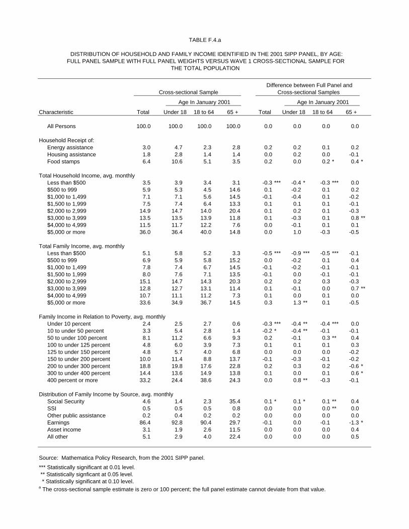
TABLE F.4.a

DISTRIBUTION OF HOUSEHOLD AND FAMILY INCOME IDENTIFIED IN THE 2001 SIPP PANEL, BY AGE:FULL PANEL SAMPLE WITH FULL PANEL WEIGHTS VERSUS WAVE 1 CROSS-SECTIONAL SAMPLE FOR

THE TOTAL POPULATION

Difference between Full Panel and Cross-sectional Sample Cross-sectional Samples

Age In January 2001 Age In January 2001

Characteristic Total Under 18 18 to 64 65 + Total Under 18 18 to 64 65 +

All Persons 100.0 100.0 100.0 100.0 0.0 0.0 0.0 0.0

Household Receipt of:Energy assistance 3.0 4.7 2.3 2.8 0.2 0.2 0.1 0.2 Housing assistance 1.8 2.8 1.4 1.4 0.0 0.2 0.0 -0.1 Food stamps 6.4 10.6 5.1 3.5 0.2 0.0 0.2 * 0.4 *

Total Household Income, avg. monthlyLess than $500 3.5 3.9 3.4 3.1 -0.3 *** -0.4 * -0.3 *** 0.0 $500 to 999 5.9 5.3 4.5 14.6 0.1 -0.2 0.1 0.2 $1,000 to 1,499 7.1 7.1 5.6 14.5 -0.1 -0.4 0.1 -0.2 $1,500 to 1,999 7.5 7.4 6.4 13.3 0.1 0.1 0.1 -0.1 $2,000 to 2,999 14.9 14.7 14.0 20.4 0.1 0.2 0.1 -0.3 $3,000 to 3,999 13.5 13.5 13.9 11.8 0.1 -0.3 0.1 0.8 **$4,000 to 4,999 11.5 11.7 12.2 7.6 0.0 -0.1 0.1 0.1 $5,000 or more 36.0 36.4 40.0 14.8 0.0 1.0 -0.3 -0.5

Total Family Income, avg. monthlyLess than $500 5.1 5.8 5.2 3.3 -0.5 *** -0.9 *** -0.5 *** -0.1 $500 to 999 6.9 5.9 5.8 15.2 0.0 -0.2 0.1 0.4 $1,000 to 1,499 7.8 7.4 6.7 14.5 -0.1 -0.2 -0.1 -0.1 $1,500 to 1,999 8.0 7.6 7.1 13.5 -0.1 0.0 -0.1 -0.1 $2,000 to 2,999 15.1 14.7 14.3 20.3 0.2 0.2 0.3 -0.3 $3,000 to 3,999 12.8 12.7 13.1 11.4 0.1 -0.1 0.0 0.7 **$4,000 to 4,999 10.7 11.1 11.2 7.3 0.1 0.0 0.1 0.0 $5,000 or more 33.6 34.9 36.7 14.5 0.3 1.3 ** 0.1 -0.5

Family Income in Relation to Poverty, avg. monthlyUnder 10 percent 2.4 2.5 2.7 0.6 -0.3 *** -0.4 ** -0.4 *** 0.0 10 to under 50 percent 3.3 5.4 2.8 1.4 -0.2 * -0.4 ** -0.1 -0.1 50 to under 100 percent 8.1 11.2 6.6 9.3 0.2 -0.1 0.3 ** 0.4 100 to under 125 percent 4.8 6.0 3.9 7.3 0.1 0.1 0.1 0.3 125 to under 150 percent 4.8 5.7 4.0 6.8 0.0 0.0 0.0 -0.2 150 to under 200 percent 10.0 11.4 8.8 13.7 -0.1 -0.3 -0.1 -0.2 200 to under 300 percent 18.8 19.8 17.6 22.8 0.2 0.3 0.2 -0.6 *300 to under 400 percent 14.4 13.6 14.9 13.8 0.1 0.0 0.1 0.6 *400 percent or more 33.2 24.4 38.6 24.3 0.0 0.8 ** -0.3 -0.1

Distribution of Family Income by Source, avg. monthlySocial Security 4.6 1.4 2.3 35.4 0.1 * 0.1 * 0.1 ** 0.4 SSI 0.5 0.5 0.5 0.8 0.0 0.0 0.0 ** 0.0 Other public assistance 0.2 0.4 0.2 0.2 0.0 0.0 0.0 0.0 Earnings 86.4 92.8 90.4 29.7 -0.1 0.0 -0.1 -1.3 *Asset income 3.1 1.9 2.6 11.5 0.0 0.0 0.0 0.4 All other 5.1 2.9 4.0 22.4 0.0 0.0 0.0 0.5

Source: Mathematica Policy Research, from the 2001 SIPP panel.

*** Statistically significant at 0.01 level. ** Statistically signficant at 0.05 level. * Statistically significant at 0.10 level.a The cross-sectional sample estimate is zero or 100 percent; the full panel estimate cannot deviate from that value.

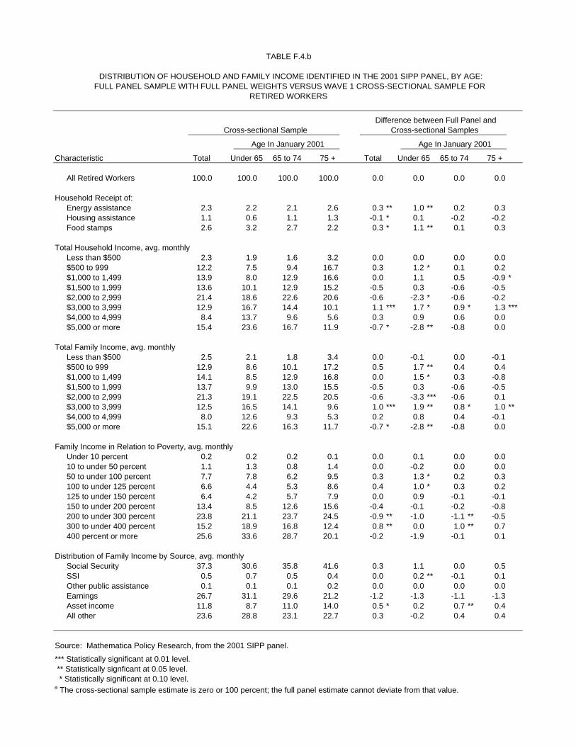
TABLE F.4.b

DISTRIBUTION OF HOUSEHOLD AND FAMILY INCOME IDENTIFIED IN THE 2001 SIPP PANEL, BY AGE:FULL PANEL SAMPLE WITH FULL PANEL WEIGHTS VERSUS WAVE 1 CROSS-SECTIONAL SAMPLE FOR

RETIRED WORKERS

Difference between Full Panel and Cross-sectional Sample Cross-sectional Samples

Age In January 2001 Age In January 2001

Characteristic Total Under 65 65 to 74 75 + Total Under 65 65 to 74 75 +

All Retired Workers 100.0 100.0 100.0 100.0 0.0 0.0 0.0 0.0

Household Receipt of:Energy assistance 2.3 2.2 2.1 2.6 0.3 ** 1.0 ** 0.2 0.3 Housing assistance 1.1 0.6 1.1 1.3 -0.1 * 0.1 -0.2 -0.2 Food stamps 2.6 3.2 2.7 2.2 0.3 * 1.1 ** 0.1 0.3

Total Household Income, avg. monthlyLess than $500 2.3 1.9 1.6 3.2 0.0 0.0 0.0 0.0 $500 to 999 12.2 7.5 9.4 16.7 0.3 1.2 * 0.1 0.2 $1,000 to 1,499 13.9 8.0 12.9 16.6 0.0 1.1 0.5 -0.9 *$1,500 to 1,999 13.6 10.1 12.9 15.2 -0.5 0.3 -0.6 -0.5 $2,000 to 2,999 21.4 18.6 22.6 20.6 -0.6 -2.3 * -0.6 -0.2 $3,000 to 3,999 12.9 16.7 14.4 10.1 1.1 *** 1.7 * 0.9 * 1.3 ***$4,000 to 4,999 8.4 13.7 9.6 5.6 0.3 0.9 0.6 0.0 $5,000 or more 15.4 23.6 16.7 11.9 -0.7 * -2.8 ** -0.8 0.0

Total Family Income, avg. monthlyLess than $500 2.5 2.1 1.8 3.4 0.0 -0.1 0.0 -0.1 $500 to 999 12.9 8.6 10.1 17.2 0.5 1.7 ** 0.4 0.4 $1,000 to 1,499 14.1 8.5 12.9 16.8 0.0 1.5 * 0.3 -0.8 $1,500 to 1,999 13.7 9.9 13.0 15.5 -0.5 0.3 -0.6 -0.5 $2,000 to 2,999 21.3 19.1 22.5 20.5 -0.6 -3.3 *** -0.6 0.1 $3,000 to 3,999 12.5 16.5 14.1 9.6 1.0 *** 1.9 ** 0.8 * 1.0 **$4,000 to 4,999 8.0 12.6 9.3 5.3 0.2 0.8 0.4 -0.1 $5,000 or more 15.1 22.6 16.3 11.7 -0.7 * -2.8 ** -0.8 0.0

Family Income in Relation to Poverty, avg. monthlyUnder 10 percent 0.2 0.2 0.2 0.1 0.0 0.1 0.0 0.0 10 to under 50 percent 1.1 1.3 0.8 1.4 0.0 -0.2 0.0 0.0 50 to under 100 percent 7.7 7.8 6.2 9.5 0.3 1.3 * 0.2 0.3 100 to under 125 percent 6.6 4.4 5.3 8.6 0.4 1.0 * 0.3 0.2 125 to under 150 percent 6.4 4.2 5.7 7.9 0.0 0.9 -0.1 -0.1 150 to under 200 percent 13.4 8.5 12.6 15.6 -0.4 -0.1 -0.2 -0.8 200 to under 300 percent 23.8 21.1 23.7 24.5 -0.9 ** -1.0 -1.1 ** -0.5 300 to under 400 percent 15.2 18.9 16.8 12.4 0.8 ** 0.0 1.0 ** 0.7 400 percent or more 25.6 33.6 28.7 20.1 -0.2 -1.9 -0.1 0.1

Distribution of Family Income by Source, avg. monthlySocial Security 37.3 30.6 35.8 41.6 0.3 1.1 0.0 0.5 SSI 0.5 0.7 0.5 0.4 0.0 0.2 ** -0.1 0.1 Other public assistance 0.1 0.1 0.1 0.2 0.0 0.0 0.0 0.0 Earnings 26.7 31.1 29.6 21.2 -1.2 -1.3 -1.1 -1.3 Asset income 11.8 8.7 11.0 14.0 0.5 * 0.2 0.7 ** 0.4 All other 23.6 28.8 23.1 22.7 0.3 -0.2 0.4 0.4

Source: Mathematica Policy Research, from the 2001 SIPP panel.

*** Statistically significant at 0.01 level. ** Statistically signficant at 0.05 level. * Statistically significant at 0.10 level.a The cross-sectional sample estimate is zero or 100 percent; the full panel estimate cannot deviate from that value.

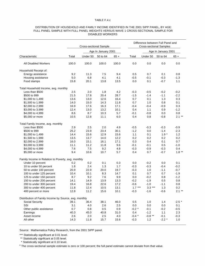
TABLE F.4.c

DISTRIBUTION OF HOUSEHOLD AND FAMILY INCOME IDENTIFIED IN THE 2001 SIPP PANEL, BY AGE:FULL PANEL SAMPLE WITH FULL PANEL WEIGHTS VERSUS WAVE 1 CROSS-SECTIONAL SAMPLE FOR

DISABLED WORKERS

Difference between Full Panel and Cross-sectional Sample Cross-sectional Samples

Age In January 2001 Age In January 2001

Characteristic Total Under 50 50 to 64 65 + Total Under 50 50 to 64 65 +

All Disabled Workers 100.0 100.0 100.0 100.0 0.0 0.0 0.0 0.0

Household Receipt of:Energy assistance 9.2 11.3 7.5 9.4 0.5 0.7 0.1 0.8 Housing assistance 5.0 6.8 4.1 4.1 -0.5 -0.1 -0.3 -1.3 Food stamps 15.8 20.1 13.8 13.5 0.0 0.1 -0.7 1.1

Total Household Income, avg. monthlyLess than $500 2.5 2.0 1.8 4.2 -0.3 -0.5 -0.2 -0.2 $500 to 999 21.5 17.8 20.4 28.7 -1.5 -1.4 -1.1 -2.2 $1,000 to 1,499 13.6 13.0 12.6 16.4 0.7 0.1 1.3 0.3 $1,500 to 1,999 14.0 15.0 14.3 11.8 0.7 1.0 0.8 0.1 $2,000 to 2,999 16.9 17.6 16.3 17.1 -0.4 -0.4 -0.9 0.3 $3,000 to 3,999 12.4 13.0 13.2 10.1 0.4 1.1 0.9 -1.2 $4,000 to 4,999 8.6 8.7 10.3 5.7 -0.1 -0.8 0.0 0.8 $5,000 or more 10.5 12.8 11.1 6.0 0.4 0.8 -0.8 2.1 **

Total Family Income, avg. monthlyLess than $500 2.9 2.5 2.0 4.9 -0.5 -0.3 -0.3 -0.9 $500 to 999 25.2 23.9 23.4 30.1 -1.2 0.0 -1.4 -2.3 $1,000 to 1,499 14.4 15.6 12.9 15.6 1.1 0.1 1.9 * 1.2 $1,500 to 1,999 13.5 13.7 14.0 12.2 0.2 0.2 0.2 0.2 $2,000 to 2,999 16.0 15.1 16.1 17.1 0.3 0.4 0.1 0.7 $3,000 to 3,999 11.1 11.2 11.8 9.6 -0.1 -0.1 0.5 -1.0 $4,000 to 4,999 7.6 7.5 9.2 4.8 -0.3 -0.9 -0.3 0.4 $5,000 or more 9.4 10.6 10.7 5.7 0.4 0.7 -0.7 1.8 **

Family Income in Relation to Poverty, avg. monthlyUnder 10 percent 0.2 0.2 0.1 0.3 0.0 -0.2 0.0 0.1 10 to under 50 percent 1.8 2.4 1.3 1.7 -0.3 -0.3 -0.4 -0.2 50 to under 100 percent 20.9 22.9 20.0 19.7 -0.3 1.0 -1.1 -0.7 100 to under 125 percent 10.4 10.1 8.3 14.7 0.1 0.7 0.7 -1.9 125 to under 150 percent 8.7 9.2 7.6 9.9 0.0 -0.2 0.8 -1.2 150 to under 200 percent 14.1 14.9 13.9 13.3 -0.2 -1.9 0.5 0.8 200 to under 300 percent 19.4 16.8 22.6 17.2 -0.6 -1.0 -1.1 0.8 300 to under 400 percent 11.8 12.4 10.5 13.1 1.7 *** 3.3 *** 1.3 0.2 400 percent or more 12.8 11.2 15.6 10.1 -0.3 -1.6 -0.6 2.1 **

Distribution of Family Income by Source, avg. monthlySocial Security 39.1 36.4 38.1 46.0 0.5 1.0 1.4 -2.5 *SSI 3.1 4.0 2.6 2.5 0.0 0.0 0.0 0.1 Other public assistance 0.7 0.8 0.5 0.9 -0.2 * -0.1 -0.2 -0.5 Earnings 40.3 45.0 40.8 31.0 0.4 -1.2 1.1 2.3 Asset income 2.6 2.0 2.5 4.0 -0.4 * -0.8 ** -0.1 -0.3 All other 14.3 11.8 15.7 15.6 -0.3 1.2 -2.2 * 1.0

Source: Mathematica Policy Research, from the 2001 SIPP panel.

*** Statistically significant at 0.01 level. ** Statistically signficant at 0.05 level. * Statistically significant at 0.10 level.a The cross-sectional sample estimate is zero or 100 percent; the full panel estimate cannot deviate from that value.

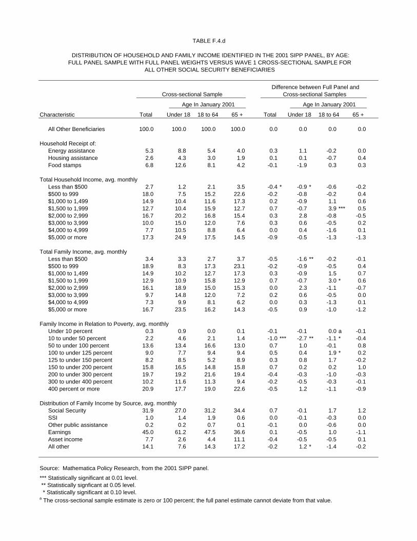
TABLE F.4.d

DISTRIBUTION OF HOUSEHOLD AND FAMILY INCOME IDENTIFIED IN THE 2001 SIPP PANEL, BY AGE:FULL PANEL SAMPLE WITH FULL PANEL WEIGHTS VERSUS WAVE 1 CROSS-SECTIONAL SAMPLE FOR

ALL OTHER SOCIAL SECURITY BENEFICIARIES

Difference between Full Panel and Cross-sectional Sample Cross-sectional Samples

Age In January 2001 Age In January 2001

Characteristic Total Under 18 18 to 64 65 + Total Under 18 18 to 64 65 +

All Other Beneficiaries 100.0 100.0 100.0 100.0 0.0 0.0 0.0 0.0

Household Receipt of:Energy assistance 5.3 8.8 5.4 4.0 0.3 1.1 -0.2 0.0 Housing assistance 2.6 4.3 3.0 1.9 0.1 0.1 -0.7 0.4 Food stamps 6.8 12.6 8.1 4.2 -0.1 -1.9 0.3 0.3

Total Household Income, avg. monthlyLess than $500 2.7 1.2 2.1 3.5 -0.4 * -0.9 * -0.6 -0.2 $500 to 999 18.0 7.5 15.2 22.6 -0.2 -0.8 -0.2 0.4 $1,000 to 1,499 14.9 10.4 11.6 17.3 0.2 -0.9 1.1 0.6 $1,500 to 1,999 12.7 10.4 15.9 12.7 0.7 -0.7 3.9 *** 0.5 $2,000 to 2,999 16.7 20.2 16.8 15.4 0.3 2.8 -0.8 -0.5 $3,000 to 3,999 10.0 15.0 12.0 7.6 0.3 0.6 -0.5 0.2 $4,000 to 4,999 7.7 10.5 8.8 6.4 0.0 0.4 -1.6 0.1 $5,000 or more 17.3 24.9 17.5 14.5 -0.9 -0.5 -1.3 -1.3

Total Family Income, avg. monthlyLess than $500 3.4 3.3 2.7 3.7 -0.5 -1.6 ** -0.2 -0.1 $500 to 999 18.9 8.3 17.3 23.1 -0.2 -0.9 -0.5 0.4 $1,000 to 1,499 14.9 10.2 12.7 17.3 0.3 -0.9 1.5 0.7 $1,500 to 1,999 12.9 10.9 15.8 12.9 0.7 -0.7 3.0 * 0.6 $2,000 to 2,999 16.1 18.9 15.0 15.3 0.0 2.3 -1.1 -0.7 $3,000 to 3,999 9.7 14.8 12.0 7.2 0.2 0.6 -0.5 0.0 $4,000 to 4,999 7.3 9.9 8.1 6.2 0.0 0.3 -1.3 0.1 $5,000 or more 16.7 23.5 16.2 14.3 -0.5 0.9 -1.0 -1.2

Family Income in Relation to Poverty, avg. monthlyUnder 10 percent 0.3 0.9 0.0 0.1 -0.1 -0.1 0.0 a -0.1 10 to under 50 percent 2.2 4.6 2.1 1.4 -1.0 *** -2.7 ** -1.1 * -0.4 50 to under 100 percent 13.6 13.4 16.6 13.0 0.7 1.0 -0.1 0.8 100 to under 125 percent 9.0 7.7 9.4 9.4 0.5 0.4 1.9 * 0.2 125 to under 150 percent 8.2 8.5 5.2 8.9 0.3 0.8 1.7 -0.2 150 to under 200 percent 15.8 16.5 14.8 15.8 0.7 0.2 0.2 1.0 200 to under 300 percent 19.7 19.2 21.6 19.4 -0.4 -0.3 -1.0 -0.3 300 to under 400 percent 10.2 11.6 11.3 9.4 -0.2 -0.5 -0.3 -0.1 400 percent or more 20.9 17.7 19.0 22.6 -0.5 1.2 -1.1 -0.9

Distribution of Family Income by Source, avg. monthlySocial Security 31.9 27.0 31.2 34.4 0.7 -0.1 1.7 1.2 SSI 1.0 1.4 1.9 0.6 0.0 -0.1 -0.3 0.0 Other public assistance 0.2 0.2 0.7 0.1 -0.1 0.0 -0.6 0.0 Earnings 45.0 61.2 47.5 36.6 0.1 -0.5 1.0 -1.1 Asset income 7.7 2.6 4.4 11.1 -0.4 -0.5 -0.5 0.1 All other 14.1 7.6 14.3 17.2 -0.2 1.2 * -1.4 -0.2

Source: Mathematica Policy Research, from the 2001 SIPP panel.

*** Statistically significant at 0.01 level. ** Statistically signficant at 0.05 level. * Statistically significant at 0.10 level.a The cross-sectional sample estimate is zero or 100 percent; the full panel estimate cannot deviate from that value.

TABLE F.4.e

DISTRIBUTION OF HOUSEHOLD AND FAMILY INCOME IDENTIFIED IN THE 2001 SIPP PANEL, BY AGE:FULL PANEL SAMPLE WITH FULL PANEL WEIGHTS VERSUS WAVE 1 CROSS-SECTIONAL SAMPLE FOR

SSI RECIPIENTS

Difference between Full Panel and Cross-sectional Sample Cross-sectional Samples

Age In January 2001 Age In January 2001

Characteristic Total Under 18 18 to 64 65 + Total Under 18 18 to 64 65 +

All SSI Recipients 100.0 100.0 100.0 100.0 0.0 0.0 0.0 0.0

Household Receipt of:Energy assistance 17.7 13.0 18.6 17.9 0.5 -1.8 1.4 -1.7 Housing assistance 10.4 4.9 11.6 10.2 -0.1 -3.1 * 0.9 -2.0 Food stamps 36.9 27.4 38.7 37.2 1.8 -1.4 1.2 3.6 *

Total Household Income, avg. monthlyLess than $500 3.5 3.4 3.0 5.0 -0.7 -0.9 -0.6 -0.7 $500 to 999 33.8 10.6 32.5 50.3 3.2 *** 0.2 2.5 ** 3.9 *$1,000 to 1,499 15.6 17.2 15.9 14.0 -2.7 *** -7.8 ** -1.2 -4.3 ***$1,500 to 1,999 11.1 14.8 11.7 7.4 0.8 -1.9 1.5 0.6 $2,000 to 2,999 13.1 24.5 12.7 7.7 0.7 6.2 0.2 1.0 $3,000 to 3,999 8.3 14.9 8.3 4.5 -0.8 3.3 -1.4 * -0.2 $4,000 to 4,999 6.0 5.4 6.2 5.7 -0.2 -1.0 0.1 -0.8 $5,000 or more 8.7 9.3 9.7 5.5 -0.4 1.9 -1.1 0.5

Total Family Income, avg. monthlyLess than $500 4.3 6.0 3.7 5.2 -0.9 ** -1.8 -0.8 -0.9 $500 to 999 39.5 13.2 40.6 51.2 3.2 *** -1.7 2.7 ** 4.1 *$1,000 to 1,499 15.2 16.8 15.4 13.7 -2.0 ** -5.3 * -0.7 -4.0 ***$1,500 to 1,999 10.1 14.7 10.1 7.4 0.2 -3.0 0.7 0.6 $2,000 to 2,999 11.5 23.8 10.5 7.7 0.5 6.6 * -0.1 1.1 $3,000 to 3,999 7.1 12.6 7.0 4.4 -0.9 2.5 -1.4 * -0.4 $4,000 to 4,999 4.8 5.0 4.5 5.3 -0.3 -0.6 -0.1 -0.9 $5,000 or more 7.4 7.9 8.1 5.2 0.2 3.3 -0.3 0.4

Family Income in Relation to Poverty, avg. monthlyUnder 10 percent 0.1 0.5 0.0 0.0 -0.1 -0.5 0.0 a 0.0 a10 to under 50 percent 5.1 11.3 5.0 2.0 -0.9 * -3.2 -0.7 0.1 50 to under 100 percent 39.7 18.8 42.0 44.8 2.1 * -5.9 ** 2.3 * 2.4 100 to under 125 percent 11.2 14.7 9.5 13.7 -0.5 -1.0 -0.6 0.2 125 to under 150 percent 8.7 11.9 7.9 9.2 -0.8 1.6 0.1 -4.2 ***150 to under 200 percent 11.9 18.2 11.7 9.0 -0.3 -0.7 -0.5 1.2 200 to under 300 percent 12.1 13.1 12.2 11.4 0.8 6.7 ** 0.1 0.5 300 to under 400 percent 4.4 5.8 4.6 3.1 -0.3 0.8 -0.5 0.0 400 percent or more 6.8 5.8 7.0 6.7 0.0 2.0 -0.2 -0.2

Distribution of Family Income by Source, avg. monthlySocial Security 14.4 6.6 13.7 22.8 0.0 0.2 -0.1 -0.5 SSI 27.8 28.7 28.5 24.9 -1.0 -3.1 -0.3 -1.9 Other public assistance 1.9 2.0 2.0 1.4 0.0 -0.2 -0.1 0.4 Earnings 47.2 56.6 46.1 43.4 0.5 2.0 -0.2 2.4 Asset income 1.4 1.0 1.6 1.3 0.4 1.4 0.2 0.4 All other 7.3 5.1 8.1 6.2 0.2 -0.4 0.5 -0.7

Source: Mathematica Policy Research, from the 2001 SIPP panel.

*** Statistically significant at 0.01 level. ** Statistically signficant at 0.05 level. * Statistically significant at 0.10 level.a The cross-sectional sample estimate is zero or 100 percent; the full panel estimate cannot deviate from that value.

G-1

APPENDIX G

COMPARISON OF FULL PANEL AND CROSS-SECTION SAMPLES: 1996 SIPP PANEL

TABLE G.1.a

DISTRIBUTION OF PERSONAL CHARACTERISTICS IDENTIFIED IN THE 1996 SIPP PANEL, BY AGE:FULL PANEL SAMPLE WITH FULL PANEL WEIGHTS VERSUS WAVE 1 CROSS-SECTIONAL SAMPLE FOR

THE TOTAL POPULATION

Difference between Full Panel and Cross-sectional Sample Cross-sectional Samples

Age In March 1996 Age In March 1996

Characteristic Total Under 18 18 to 64 65 + Total Under 18 18 to 64 65 +

All Persons 100.0 100.0 100.0 100.0 0.0 0.0 0.0 0.0

SexMale 48.9 51.2 49.2 41.9 0.0 0.0 0.0 0.0 Female 51.1 48.8 50.8 58.1 0.0 0.0 0.0 0.0

RaceWhite 82.5 78.6 83.0 89.1 -0.2 ** -0.8 *** 0.0 -0.5 **Black 12.8 16.2 12.2 8.2 0.0 0.4 ** -0.2 ** 0.1 American Indian, Alaska Native 1.1 1.5 1.1 0.6 -0.1 0.0 -0.1 0.1 Asian, Pacific Islander 3.5 3.7 3.7 2.0 0.3 *** 0.4 *** 0.3 ** 0.4 ***

EthnicityHispanic 10.7 14.4 10.4 4.5 0.0 -0.1 * 0.0 0.2 Non-Hispanic 89.3 85.6 89.6 95.5 0.0 0.1 * 0.0 -0.2

Marital StatusMarried 42.3 0.1 58.6 54.4 0.6 *** 0.0 1.4 *** -1.2 ***Widowed 5.3 0.0 2.0 33.9 0.1 * 0.0 0.0 0.9 **Divorced or separated 9.1 0.1 13.4 7.4 -0.4 *** 0.0 -0.7 *** 0.1 Never married 43.3 99.8 25.9 4.4 -0.3 *** 0.0 -0.7 *** 0.3

Years of education0 to 8 6.1 2.4 5.0 20.4 0.4 *** 0.1 0.4 *** 1.5 ***9 to 11 10.3 13.0 8.5 13.7 -0.1 0.4 ** -0.3 *** 0.1 12 24.8 1.4 33.5 33.6 -0.8 *** -0.1 -0.9 *** -1.1 ***13 to 15 21.1 0.1 30.8 19.1 0.4 *** 0.0 0.8 *** -0.1 16 or more 15.2 0.0 22.3 13.2 0.0 0.0 a 0.1 -0.3 Unknown (used for children) 22.4 83.2 0.0 0.0 0.0 -0.4 ** 0.0 a 0.0 a

Living ArrangementLives alone 9.5 0.0 9.4 31.6 0.0 0.0 * -0.1 * 0.4 Lives with relatives 84.7 98.9 82.0 65.9 0.5 *** 0.2 * 0.8 *** -0.6 *Lives with only non-relatives 5.8 1.1 8.5 2.4 -0.4 *** -0.1 -0.7 *** 0.2

Relationship to HouseholderHouseholder 37.7 0.2 48.4 67.0 0.0 -0.1 ** 0.1 ** 0.1 Spouse 20.3 0.0 28.5 24.0 0.4 *** 0.0 0.9 *** -0.4 **Child 32.0 89.9 12.6 0.1 0.5 *** 1.2 *** 0.2 0.0 Grandchild 1.6 5.2 0.4 0.0 0.0 -0.1 0.0 0.0 aParent 0.9 0.0 0.7 3.8 0.0 0.0 a 0.0 0.2 Sibling 1.0 0.4 1.3 0.9 -0.1 *** 0.0 -0.2 *** 0.0 Other relative 2.0 1.9 1.8 3.0 -0.5 *** -0.6 *** -0.5 *** -0.1 Nonrelative 4.6 2.3 6.3 1.4 -0.4 *** -0.4 *** -0.5 *** 0.2

Parents PresentBoth mother and father 24.3 70.6 8.7 0.0 0.9 *** 2.5 *** 0.2 0.0 Mother only 9.2 22.6 4.9 0.4 -0.2 * -1.0 *** 0.1 0.0 Father only 1.3 2.7 0.9 0.0 -0.2 *** -0.7 *** -0.1 0.0 Neither 65.3 4.1 85.5 99.5 -0.5 *** -0.8 *** -0.2 0.0

Source: Mathematica Policy Research, from the 1996 SIPP panel.

*** Statistically significant at 0.01 level. ** Statistically signficant at 0.05 level. * Statistically significant at 0.10 level.a The cross-sectional sample estimate is zero or 100 percent; the full panel estimate cannot deviate from that value.

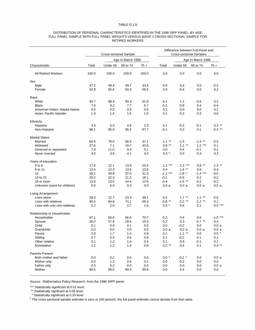
TABLE G.1.b

DISTRIBUTION OF PERSONAL CHARACTERISTICS IDENTIFIED IN THE 1996 SIPP PANEL, BY AGE:FULL PANEL SAMPLE WITH FULL PANEL WEIGHTS VERSUS WAVE 1 CROSS-SECTIONAL SAMPLE FOR

RETIRED WORKERS

Difference between Full Panel and Cross-sectional Sample Cross-sectional Samples

Age In March 1996 Age In March 1996

Characteristic Total Under 65 65 to 74 75 + Total Under 65 65 to 74 75 +

All Retired Workers 100.0 100.0 100.0 100.0 0.0 0.0 0.0 0.0

SexMale 47.2 49.4 49.7 43.5 0.0 0.4 0.0 -0.2 Female 52.8 50.6 50.3 56.5 0.0 -0.4 0.0 0.2

RaceWhite 90.7 88.9 90.3 91.8 -0.1 1.1 -0.6 0.2 Black 7.5 9.2 7.7 6.7 -0.1 -0.9 0.4 -0.4 American Indian, Alaska Native 0.5 0.5 0.5 0.6 0.1 0.0 0.0 0.2 Asian, Pacific Islander 1.3 1.4 1.5 1.0 0.1 -0.2 0.2 0.0

EthnicityHispanic 3.9 5.0 4.8 2.3 0.1 -0.2 -0.1 0.3 **Non-Hispanic 96.1 95.0 95.2 97.7 -0.1 0.2 0.1 -0.3 **

Marital StatusMarried 60.5 78.0 66.9 47.1 -1.1 ** -1.5 -1.4 ** -0.5 Widowed 27.6 7.1 19.7 43.8 0.8 ** 1.1 ** 1.2 *** 0.1 Divorced or separated 7.8 11.0 9.3 5.1 0.0 0.4 -0.1 0.1 Never married 4.0 3.9 4.1 4.0 0.3 * 0.0 0.3 0.3

Years of education0 to 8 17.8 12.1 13.9 24.5 1.2 *** 2.3 *** 0.8 ** 1.3 **9 to 11 13.4 12.3 13.5 13.6 0.4 1.6 ** 0.6 -0.4 12 35.1 39.8 37.0 31.3 -1.1 *** -1.8 * -1.4 *** -0.5 13 to 15 20.2 22.3 21.3 18.1 -0.1 -0.6 0.2 -0.2 16 or more 13.6 13.5 14.4 12.6 -0.4 -1.5 ** -0.2 -0.2 Unknown (used for children) 0.0 0.0 0.0 0.0 0.0 a 0.0 a 0.0 a 0.0 a

Living ArrangementLives alone 28.3 12.7 23.3 39.1 0.5 1.7 ** 1.1 ** -0.6 Lives with relatives 69.5 84.8 74.1 59.3 -0.8 ** -2.2 ** -1.2 ** 0.1 Lives with only non-relatives 2.2 2.5 2.7 1.6 0.3 * 0.6 0.1 0.5 ***

Relationship to HouseholderHouseholder 67.1 56.6 66.5 70.7 -0.2 0.4 0.6 -1.5 ***Spouse 26.0 37.8 28.6 19.3 -0.2 0.3 -0.7 ** 0.4 Child 0.1 0.9 0.1 0.0 0.0 -0.2 0.0 0.0 aGrandchild 0.0 0.0 0.0 0.0 0.0 a 0.0 a 0.0 a 0.0 aParent 2.8 1.7 1.4 4.9 0.1 -1.1 ** 0.0 0.5 *Sibling 0.7 0.5 0.6 0.8 0.1 -0.2 0.1 0.1 Other relative 2.1 1.3 1.4 3.4 0.1 0.3 -0.1 0.1 Nonrelative 1.2 1.2 1.4 0.9 0.2 ** 0.4 0.1 0.4 **

Parents PresentBoth mother and father 0.0 0.2 0.0 0.0 0.0 * -0.2 * 0.0 0.0 aMother only 0.5 1.1 0.6 0.1 0.0 -0.2 0.0 0.0 Father only 0.0 0.2 0.0 0.0 0.0 0.0 0.0 0.0 aNeither 99.5 98.5 99.3 99.9 0.0 0.4 0.0 0.0

Source: Mathematica Policy Research, from the 1996 SIPP panel.

*** Statistically significant at 0.01 level. ** Statistically signficant at 0.05 level. * Statistically significant at 0.10 level.a The cross-sectional sample estimate is zero or 100 percent; the full panel estimate cannot deviate from that value.

TABLE G.1.c

DISTRIBUTION OF PERSONAL CHARACTERISTICS IDENTIFIED IN THE 1996 SIPP PANEL, BY AGE:FULL PANEL SAMPLE WITH FULL PANEL WEIGHTS VERSUS WAVE 1 CROSS-SECTIONAL SAMPLE FOR

DISABLED WORKERS

Difference between Full Panel and Cross-sectional Sample Cross-sectional Samples

Age In March 1996 Age In March 1996

Characteristic Total Under 50 50 to 64 65 + Total Under 50 50 to 64 65 +

All Disabled Workers 100.0 100.0 100.0 100.0 0.0 0.0 0.0 0.0

SexMale 56.4 61.9 54.1 52.9 0.4 -0.1 -0.1 1.1 Female 43.6 38.1 45.9 47.1 -0.4 0.1 0.1 -1.1

RaceWhite 75.5 74.3 80.0 70.1 0.3 0.3 -0.3 1.6 Black 21.8 22.9 17.9 26.2 -0.5 -1.0 0.6 -1.6 American Indian, Alaska Native 1.6 1.7 1.3 2.1 0.0 0.4 -0.3 -0.1 Asian, Pacific Islander 1.1 1.1 0.8 1.6 0.2 0.3 0.1 0.2

EthnicityHispanic 6.8 6.7 6.0 8.1 -0.1 -0.3 -0.8 1.2 *Non-Hispanic 93.2 93.3 94.0 91.9 0.1 0.3 0.8 -1.2 *

Marital StatusMarried 43.2 29.5 53.2 45.1 0.8 0.7 0.9 3.0 **Widowed 14.1 2.2 12.9 30.9 -0.6 -0.3 0.7 -1.6 Divorced or separated 20.4 21.4 23.1 15.0 -2.8 *** -3.9 *** -2.9 ** -1.2 Never married 22.3 46.9 10.7 9.0 2.6 *** 3.5 ** 1.3 * -0.2

Years of education0 to 8 25.5 14.7 23.2 42.4 1.5 * 3.0 *** 0.6 1.9 9 to 11 18.9 18.0 21.0 16.7 0.4 0.4 1.8 * -1.8 12 32.2 38.7 31.0 25.8 -1.0 -0.1 -1.9 -1.7 13 to 15 18.1 21.9 19.1 11.8 -0.8 -2.8 * -0.8 1.4 16 or more 5.4 6.6 5.8 3.2 0.0 -0.5 0.4 0.2 Unknown (used for children) 0.0 0.0 0.0 0.0 0.0 a 0.0 a 0.0 a 0.0 a

Living ArrangementLives alone 23.4 19.2 22.5 30.0 -1.2 * -0.9 0.5 -3.7 ***Lives with relatives 68.6 69.4 71.2 63.6 2.1 ** 2.8 0.8 3.1 **Lives with only non-relatives 8.0 11.4 6.3 6.4 -0.9 -1.9 -1.2 0.6

Relationship to HouseholderHouseholder 59.5 49.5 64.8 64.0 -2.2 ** -3.7 * 0.1 -2.1 Spouse 17.4 12.1 21.6 17.5 1.2 ** 0.9 0.9 3.0 ***Child 8.9 22.9 2.9 0.4 1.7 *** 3.2 ** 0.1 0.0 Grandchild 0.2 0.7 0.0 0.0 0.1 0.3 0.0 a 0.0 aParent 2.4 0.2 2.1 5.4 -0.4 -0.2 -0.1 -0.7 Sibling 2.3 3.7 1.6 1.6 -0.1 0.2 -0.2 -0.5 Other relative 3.9 2.7 3.4 6.2 0.1 0.4 0.1 -0.3 Nonrelative 5.4 8.2 3.5 4.8 -0.5 -1.1 -0.9 0.6

Parents PresentBoth mother and father 5.0 13.0 1.3 0.3 0.6 0.6 0.1 0.2 Mother only 5.3 11.1 3.5 0.5 1.1 ** 2.8 *** -0.4 0.0 Father only 0.9 2.6 0.2 0.0 0.2 0.3 0.1 0.0 aNeither 88.9 73.2 95.0 99.2 -1.8 *** -3.8 *** 0.3 -0.2

Source: Mathematica Policy Research, from the 1996 SIPP panel.

*** Statistically significant at 0.01 level. ** Statistically signficant at 0.05 level. * Statistically significant at 0.10 level.a The cross-sectional sample estimate is zero or 100 percent; the full panel estimate cannot deviate from that value.

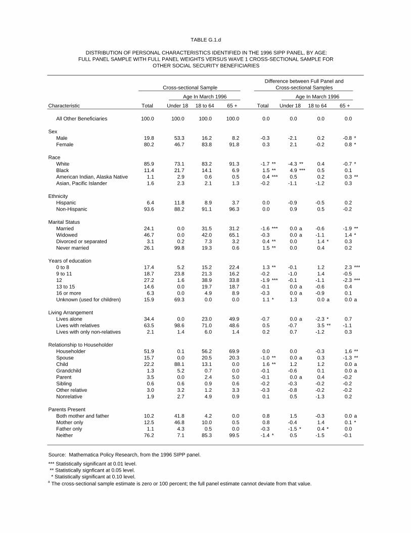
TABLE G.1.d

DISTRIBUTION OF PERSONAL CHARACTERISTICS IDENTIFIED IN THE 1996 SIPP PANEL, BY AGE:FULL PANEL SAMPLE WITH FULL PANEL WEIGHTS VERSUS WAVE 1 CROSS-SECTIONAL SAMPLE FOR

OTHER SOCIAL SECURITY BENEFICIARIES

Difference between Full Panel and Cross-sectional Sample Cross-sectional Samples

Age In March 1996 Age In March 1996

Characteristic Total Under 18 18 to 64 65 + Total Under 18 18 to 64 65 +

All Other Beneficiaries 100.0 100.0 100.0 100.0 0.0 0.0 0.0 0.0

SexMale 19.8 53.3 16.2 8.2 -0.3 -2.1 0.2 -0.8 *Female 80.2 46.7 83.8 91.8 0.3 2.1 -0.2 0.8 *

RaceWhite 85.9 73.1 83.2 91.3 -1.7 ** -4.3 ** 0.4 -0.7 *Black 11.4 21.7 14.1 6.9 1.5 ** 4.9 *** 0.5 0.1 American Indian, Alaska Native 1.1 2.9 0.6 0.5 0.4 *** 0.5 0.2 0.3 **Asian, Pacific Islander 1.6 2.3 2.1 1.3 -0.2 -1.1 -1.2 0.3

EthnicityHispanic 6.4 11.8 8.9 3.7 0.0 -0.9 -0.5 0.2 Non-Hispanic 93.6 88.2 91.1 96.3 0.0 0.9 0.5 -0.2

Marital StatusMarried 24.1 0.0 31.5 31.2 -1.6 *** 0.0 a -0.6 -1.9 **Widowed 46.7 0.0 42.0 65.1 -0.3 0.0 a -1.1 1.4 *Divorced or separated 3.1 0.2 7.3 3.2 0.4 ** 0.0 1.4 * 0.3 Never married 26.1 99.8 19.3 0.6 1.5 ** 0.0 0.4 0.2

Years of education0 to 8 17.4 5.2 15.2 22.4 1.3 ** -0.1 1.2 2.3 ***9 to 11 18.7 23.8 21.3 16.2 -0.2 -1.0 1.4 -0.5 12 27.2 1.6 38.9 33.8 -1.9 *** -0.1 -1.1 -2.3 ***13 to 15 14.6 0.0 19.7 18.7 -0.1 0.0 a -0.6 0.4 16 or more 6.3 0.0 4.9 8.9 -0.3 0.0 a -0.9 0.1 Unknown (used for children) 15.9 69.3 0.0 0.0 1.1 * 1.3 0.0 a 0.0 a

Living ArrangementLives alone 34.4 0.0 23.0 49.9 -0.7 0.0 a -2.3 * 0.7 Lives with relatives 63.5 98.6 71.0 48.6 0.5 -0.7 3.5 ** -1.1 Lives with only non-relatives 2.1 1.4 6.0 1.4 0.2 0.7 -1.2 0.3

Relationship to HouseholderHouseholder 51.9 0.1 56.2 69.9 0.0 0.0 -0.3 1.6 **Spouse 15.7 0.0 20.5 20.3 -1.0 ** 0.0 a 0.3 -1.3 **Child 22.2 88.1 13.1 0.0 1.6 ** 1.2 1.2 0.0 aGrandchild 1.3 5.2 0.7 0.0 -0.1 -0.6 0.1 0.0 aParent 3.5 0.0 2.4 5.0 -0.1 0.0 a 0.4 -0.2 Sibling 0.6 0.6 0.9 0.6 -0.2 -0.3 -0.2 -0.2 Other relative 3.0 3.2 1.2 3.3 -0.3 -0.8 -0.2 -0.2 Nonrelative 1.9 2.7 4.9 0.9 0.1 0.5 -1.3 0.2

Parents PresentBoth mother and father 10.2 41.8 4.2 0.0 0.8 1.5 -0.3 0.0 aMother only 12.5 46.8 10.0 0.5 0.8 -0.4 1.4 0.1 *Father only 1.1 4.3 0.5 0.0 -0.3 -1.5 * 0.4 * 0.0 Neither 76.2 7.1 85.3 99.5 -1.4 * 0.5 -1.5 -0.1

Source: Mathematica Policy Research, from the 1996 SIPP panel.

*** Statistically significant at 0.01 level. ** Statistically signficant at 0.05 level. * Statistically significant at 0.10 level.a The cross-sectional sample estimate is zero or 100 percent; the full panel estimate cannot deviate from that value.

TABLE G.1.e

DISTRIBUTION OF PERSONAL CHARACTERISTICS IDENTIFIED IN THE 1996 SIPP PANEL, BY AGE:FULL PANEL SAMPLE WITH FULL PANEL WEIGHTS VERSUS WAVE 1 CROSS-SECTIONAL SAMPLE FOR

SSI RECIPIENTS

Difference between Full Panel and Cross-sectional Sample Cross-sectional Samples

Age In March 1996 Age In March 1996

Characteristic Total Under 18 18 to 64 65 + Total Under 18 18 to 64 65 +

All SSI Recipients 100.0 100.0 100.0 100.0 0.0 0.0 0.0 0.0

SexMale 46.0 63.0 50.6 28.2 -1.4 -2.4 -1.8 1.1 Female 54.0 37.0 49.4 71.8 1.4 2.4 1.8 -1.1

RaceWhite 61.4 54.7 64.7 58.2 -0.3 2.7 -0.9 -0.6 Black 30.9 40.6 30.6 26.7 -0.4 -2.4 0.6 -1.0 American Indian, Alaska Native 2.2 2.2 2.3 2.2 0.4 0.7 0.1 0.8 **Asian, Pacific Islander 5.4 2.5 2.4 13.0 0.3 -1.0 0.1 0.8

EthnicityHispanic 13.3 14.2 10.5 18.6 0.4 -3.6 0.7 1.5 Non-Hispanic 86.7 85.8 89.5 81.4 -0.4 3.6 -0.7 -1.5

Marital StatusMarried 20.0 0.0 21.9 25.8 1.5 * 0.0 a 1.1 1.7 Widowed 16.5 0.0 7.6 42.6 -0.2 0.0 a -0.5 -1.4 Divorced or separated 19.9 0.3 24.3 20.6 -0.3 -0.3 -0.7 -0.7 Never married 43.7 99.7 46.2 10.9 -1.0 0.3 0.0 0.3

Years of education0 to 8 32.3 6.7 26.3 57.3 2.6 *** -0.8 2.6 ** 1.9 9 to 11 19.6 17.8 21.5 16.8 -1.1 -1.7 -1.1 -0.9 12 26.0 1.4 36.9 15.9 -0.5 1.0 -1.0 -1.1 13 to 15 9.1 0.0 12.3 7.0 0.1 0.0 a 0.0 0.2 16 or more 2.5 0.0 2.9 3.1 -0.2 0.0 a -0.4 0.0 Unknown (used for children) 10.4 74.0 0.0 0.0 -0.9 1.5 0.0 a 0.0 a

Living ArrangementLives alone 23.6 0.0 21.1 40.4 -0.7 0.0 a -1.2 -1.8 Lives with relatives 67.1 97.9 65.9 54.3 1.4 -1.6 ** 3.0 ** 1.4 Lives with only non-relatives 9.2 2.1 12.9 5.3 -0.7 1.6 ** -1.8 ** 0.4

Relationship to HouseholderHouseholder 45.7 0.0 47.9 63.7 -0.1 0.0 a -2.0 * 0.7 Spouse 8.2 0.0 9.9 8.9 0.9 ** 0.0 a 0.7 1.2 **Child 24.2 81.6 22.1 0.2 0.6 0.5 2.7 ** 0.1 Grandchild 1.6 9.3 0.6 0.0 0.0 0.6 0.1 0.0 aParent 4.1 0.0 1.8 11.0 0.2 0.0 a 0.2 0.0 Sibling 2.9 0.6 3.3 3.1 0.2 0.0 0.1 0.2 Other relative 5.9 4.0 4.6 9.3 -1.5 *** -2.4 * -0.8 -2.6 ***Nonrelative 7.4 4.5 9.9 3.8 -0.3 1.3 -1.0 0.4

Parents PresentBoth mother and father 12.1 34.6 12.5 0.2 -0.6 -4.4 0.6 0.1 Mother only 13.7 52.1 10.7 0.7 0.3 1.8 1.4 -0.1 Father only 1.0 2.5 1.1 0.0 0.4 ** 1.0 0.5 ** 0.0 aNeither 73.2 10.8 75.7 99.0 -0.1 1.6 -2.5 ** 0.0

Source: Mathematica Policy Research, from the 1996 SIPP panel.

*** Statistically significant at 0.01 level. ** Statistically signficant at 0.05 level. * Statistically significant at 0.10 level.a The cross-sectional sample estimate is zero or 100 percent; the full panel estimate cannot deviate from that value.

TABLE G.2.a

DISTRIBUTION OF ADDITIONAL PERSONAL CHARACTERISTICS IDENTIFIED IN THE 1996 SIPP PANEL, BY AGE:FULL PANEL SAMPLE WITH FULL PANEL WEIGHTS VERSUS WAVE 1 CROSS-SECTIONAL SAMPLE FOR

THE TOTAL POPULATION

Difference between Full Panel and Cross-sectional Sample Cross-sectional Samples

Age In March 1996 Age In March 1996

Characteristic Total Under 18 18 to 64 65 + Total Under 18 18 to 64 65 +

All Persons 100.0 100.0 100.0 100.0 0.0 0.0 0.0 0.0

Health InsuranceMedicaid 10.7 19.3 7.2 9.2 -0.1 -1.0 *** 0.1 1.0 ***Medicare 12.4 0.0 2.0 93.0 0.0 0.0 a 0.1 ** -0.2 Private (including military) 73.2 68.6 74.6 76.9 1.2 *** 2.3 *** 1.1 *** -0.4 None 15.3 14.6 18.4 1.0 -1.1 *** -1.2 *** -1.2 *** 0.0

Sources of Own IncomeSocial Security 14.9 3.1 4.9 92.4 0.2 ** 0.3 ** 0.2 *** -0.3 SSI 2.3 1.2 2.1 5.4 0.2 *** 0.0 0.2 *** 0.8 ***Other public assistance 1.9 0.1 2.8 1.3 0.0 0.0 -0.1 0.1 Earnings 47.0 4.2 72.9 11.4 0.4 *** 0.1 0.7 *** 0.2 Asset income 41.4 3.9 52.6 68.4 1.1 *** 0.4 *** 1.8 *** -0.6 *Other 11.0 0.1 9.4 43.7 0.1 0.0 0.0 0.6 *

Total Personal Income, avg. monthlyUnder $100 33.7 92.7 13.9 1.9 -0.3 *** -0.2 -0.5 *** -0.1 $100 to 249 3.4 2.5 4.0 2.4 0.0 0.2 -0.1 -0.1 $250 to 499 7.2 3.1 7.6 14.7 0.1 0.1 0.0 0.5 **$500 to 749 7.0 1.1 7.3 18.3 0.1 -0.1 0.2 0.3 $750 to 999 6.0 0.4 6.6 15.2 0.0 0.0 0.1 -0.5 $1,000 to 1,499 10.3 0.2 13.0 19.3 -0.2 0.0 -0.3 * 0.2 $1,500 to 1,999 8.1 0.0 11.0 11.4 0.1 * 0.0 0.3 ** -0.1 $2,000 to 2,999 11.1 0.0 16.2 9.5 0.1 0.0 * 0.2 0.0 $3,000 to 3,999 5.9 0.0 8.9 3.9 0.2 ** 0.0 0.3 ** -0.1 $4,000 to 4999 3.1 0.0 4.8 1.5 0.1 0.0 a 0.1 0.0 $5,000 or more 4.2 0.0 6.6 1.8 -0.2 *** 0.0 a -0.3 *** -0.3 ***

SSEC Payments as a Percentage ofTotal Personal Income, avg. monthly

Under 25 percent 86.4 96.9 95.5 16.2 -0.2 *** -0.2 * -0.2 *** 0.1 25 to under 50 percent 3.3 0.1 1.2 21.7 0.0 0.0 0.0 -0.2 50 to under 75 percent 3.2 0.1 1.0 21.5 0.1 ** 0.0 0.1 * 0.5 *75 to under 100 percent 4.0 0.3 1.1 26.9 0.0 0.1 0.0 -0.2 100 percent 3.1 2.6 1.2 13.7 0.1 0.2 0.1 * -0.2

Source: Mathematica Policy Research, from the 1996 SIPP panel.

*** Statistically significant at 0.01 level. ** Statistically signficant at 0.05 level. * Statistically significant at 0.10 level.a The cross-sectional sample estimate is zero or 100 percent; the full panel estimate cannot deviate from that value.

TABLE G.2.b

DISTRIBUTION OF ADDITIONAL PERSONAL CHARACTERISTICS IDENTIFIED IN THE 1996 SIPP PANEL, BY AGE:FULL PANEL SAMPLE WITH FULL PANEL WEIGHTS VERSUS WAVE 1 CROSS-SECTIONAL SAMPLE FOR

RETIRED WORKERS

Difference between Full Panel and Cross-sectional Sample Cross-sectional Samples

Age In March 1996 Age In March 1996

Characteristic Total Under 65 65 to 74 75 + Total Under 65 65 to 74 75 +

All Retired Workers 100.0 100.0 100.0 100.0 0.0 0.0 0.0 0.0

Health InsuranceMedicaid 6.3 4.1 6.3 6.9 0.4 ** 0.9 * 0.7 *** -0.1 Medicare 91.0 16.7 100.0 100.0 0.0 -1.8 * 0.0 0.0 aPrivate (including military) 79.8 81.8 80.4 78.6 0.1 -0.6 0.1 0.2 None 1.1 10.4 0.0 0.0 0.0 -0.2 0.0 0.0 a

Sources of Own IncomeSocial Security 100.0 100.0 100.0 100.0 0.0 a 0.0 a 0.0 a 0.0 aSSI 2.8 1.4 3.0 3.0 0.4 *** 0.7 * 0.4 ** 0.2 Other public assistance 0.9 0.7 0.9 0.9 0.2 *** 0.3 * 0.1 0.2 **Earnings 10.9 17.4 14.7 3.9 0.6 *** 2.3 ** 0.7 * 0.2 Asset income 70.8 65.0 71.5 71.5 -0.1 0.2 -0.3 0.0 Other 47.9 46.8 49.6 45.9 0.6 -0.2 0.6 0.9

Total Personal Income, avg. monthlyUnder $100 0.3 0.2 0.4 0.2 0.0 0.1 0.0 -0.1 $100 to 249 1.9 2.5 2.0 1.8 0.0 -0.2 0.1 -0.1 $250 to 499 13.6 14.8 13.8 13.0 0.3 -0.9 0.1 0.9 **$500 to 749 18.0 19.3 16.4 19.7 0.2 0.7 0.4 -0.2 $750 to 999 15.7 9.9 14.3 19.2 -0.4 -0.1 -0.4 -0.6 $1,000 to 1,499 20.3 15.8 20.2 21.8 0.2 0.0 0.4 0.1 $1,500 to 1,999 12.5 13.8 13.6 10.8 0.0 0.7 -0.5 0.5 $2,000 to 2,999 10.7 15.1 11.8 8.0 -0.1 0.1 0.2 -0.4 $3,000 to 3,999 4.1 4.8 4.6 3.3 -0.1 -0.3 -0.1 0.1 $4,000 to 4999 1.6 2.7 1.6 1.2 0.0 0.1 0.0 0.0 $5,000 or more 1.3 1.1 1.5 1.1 -0.2 * -0.2 -0.2 -0.1

SSEC Payments as a Percentage ofTotal Personal Income, avg. monthly

Under 25 percent 9.7 14.3 10.7 7.2 -0.1 -0.4 -0.1 -0.1 25 to under 50 percent 24.9 31.5 27.9 19.0 0.1 2.8 ** -0.2 -0.3 50 to under 75 percent 23.2 17.7 23.9 23.9 0.4 -0.9 0.3 0.9 *75 to under 100 percent 28.1 20.6 25.0 34.3 -0.1 -1.3 -0.1 0.2 100 percent 14.0 15.9 12.4 15.6 -0.3 -0.2 0.0 -0.6

Source: Mathematica Policy Research, from the 1996 SIPP panel.

*** Statistically significant at 0.01 level. ** Statistically signficant at 0.05 level. * Statistically significant at 0.10 level.a The cross-sectional sample estimate is zero or 100 percent; the full panel estimate cannot deviate from that value.

TABLE G.2.c

DISTRIBUTION OF ADDITIONAL PERSONAL CHARACTERISTICS IDENTIFIED IN THE 1996 SIPP PANEL, BY AGE:FULL PANEL SAMPLE WITH FULL PANEL WEIGHTS VERSUS WAVE 1 CROSS-SECTIONAL SAMPLE FOR

DISABLED WORKERS

Difference between Full Panel and Cross-sectional Sample Cross-sectional Samples

Age In March 1996 Age In March 1996

Characteristic Total Under 50 50 to 64 65 + Total Under 50 50 to 64 65 +

All Disabled Workers 100.0 100.0 100.0 100.0 0.0 0.0 0.0 0.0

Health InsuranceMedicaid 35.8 49.0 27.8 31.2 0.9 0.8 0.2 0.3 Medicare 76.6 64.0 71.8 100.0 -0.2 -0.6 0.8 0.0 aPrivate (including military) 39.9 26.8 47.0 45.6 -0.7 1.2 -1.6 -0.1 None 5.1 7.8 6.1 0.0 0.2 -1.1 1.4 ** 0.0 a

Sources of Own IncomeSocial Security 100.0 100.0 100.0 100.0 0.0 a 0.0 a 0.0 a 0.0 aSSI 21.2 29.9 14.1 21.0 0.5 -0.4 0.3 0.8 Other public assistance 5.1 6.8 3.5 5.4 0.0 0.8 -1.0 0.2 Earnings 8.3 15.9 4.8 4.0 0.9 0.6 0.5 0.6 Asset income 33.9 22.8 39.8 39.1 -0.1 1.5 -1.1 0.6 Other 26.6 15.1 34.2 29.7 -1.5 ** -1.1 -1.9 0.0

Total Personal Income, avg. monthlyUnder $100 0.6 1.0 0.2 0.5 0.2 * 0.6 ** -0.2 0.2 $100 to 249 2.3 3.3 1.3 2.4 0.0 0.3 0.0 -0.6 $250 to 499 21.4 23.5 19.4 21.6 1.7 ** 2.5 0.5 2.2 *$500 to 749 31.0 34.7 26.6 32.9 0.3 -0.7 2.3 * -1.8 $750 to 999 15.2 14.6 16.0 14.6 -0.4 -0.6 -0.6 0.3 $1,000 to 1,499 15.5 12.2 18.5 15.1 -0.3 -0.7 -0.1 0.6 $1,500 to 1,999 7.2 5.5 9.1 6.5 -1.0 ** -1.6 ** -0.7 -0.3 $2,000 to 2,999 4.7 3.7 6.1 4.0 -0.4 0.2 -0.9 -0.4 $3,000 to 3,999 1.6 0.8 2.1 2.0 -0.1 0.4 * -0.3 -0.2 $4,000 to 4999 0.2 0.3 0.3 0.0 -0.1 -0.3 -0.1 0.0 a$5,000 or more 0.4 0.3 0.4 0.4 0.0 -0.1 0.2 0.0

SSEC Payments as a Percentage ofTotal Personal Income, avg. monthly

Under 25 percent 4.9 5.7 3.9 5.3 -0.2 -0.4 0.0 -0.5 25 to under 50 percent 16.2 15.9 16.9 15.5 -0.8 -2.2 * -0.5 0.9 50 to under 75 percent 21.4 20.1 20.8 24.1 0.2 0.7 0.5 -0.8 75 to under 100 percent 27.0 24.6 27.6 29.2 0.5 1.3 -0.4 1.0 100 percent 30.6 33.8 30.8 26.1 0.3 0.5 0.4 -0.6

Source: Mathematica Policy Research, from the 1996 SIPP panel.

*** Statistically significant at 0.01 level. ** Statistically signficant at 0.05 level. * Statistically significant at 0.10 level.a The cross-sectional sample estimate is zero or 100 percent; the full panel estimate cannot deviate from that value.

TABLE G.2.d

DISTRIBUTION OF ADDITIONAL PERSONAL CHARACTERISTICS IDENTIFIED IN THE 1996 SIPP PANEL, BY AGE:FULL PANEL SAMPLE WITH FULL PANEL WEIGHTS VERSUS WAVE 1 CROSS-SECTIONAL SAMPLE FOR

ALL OTHER SOCIAL SECURITY BENEFICIARIES

Difference between Full Panel and Cross-sectional Sample Cross-sectional Samples

Age In March 1996 Age In March 1996

Characteristic Total Under 18 18 to 64 65 + Total Under 18 18 to 64 65 +

All Other Beneficiaries 100.0 100.0 100.0 100.0 0.0 0.0 0.0 0.0

Health InsuranceMedicaid 15.4 27.9 20.3 9.5 1.6 *** 0.8 1.1 1.5 ***Medicare 64.6 0.0 18.2 100.0 -1.8 ** 0.0 a 0.4 0.0 aPrivate (including military) 68.4 51.7 56.9 77.3 -0.9 0.4 -1.3 -0.6 None 8.5 22.9 21.2 0.0 0.1 -2.2 1.0 0.0 a

Sources of Own IncomeSocial Security 100.0 100.0 100.0 100.0 0.0 a 0.0 a 0.0 a 0.0 aSSI 5.3 3.6 8.1 5.2 0.9 *** 0.6 0.5 1.1 ***Other public assistance 1.5 0.0 4.6 1.4 0.1 0.0 a 1.0 -0.2 Earnings 11.9 5.0 29.9 10.0 0.0 0.2 -1.4 0.1 Asset income 49.5 6.7 42.3 67.2 -0.7 1.1 -0.5 0.1 Other 22.8 0.4 21.5 31.3 -0.4 0.0 0.7 0.0

Total Personal Income, avg. monthlyUnder $100 4.5 17.7 1.7 0.3 1.0 ** 2.9 * 0.2 0.1 $100 to 249 8.7 24.3 7.4 3.2 -0.2 -1.4 0.8 -0.5 *$250 to 499 21.6 31.1 22.5 17.9 -0.1 -0.6 -0.9 0.0 $500 to 749 20.9 19.3 20.1 21.8 0.3 -1.1 -0.8 1.2 *$750 to 999 13.7 5.8 11.7 17.1 -0.4 -0.2 2.5 ** -1.0 $1,000 to 1,499 14.3 1.7 18.2 18.0 -0.3 0.5 0.1 -0.5 $1,500 to 1,999 6.9 0.2 7.8 9.2 -0.3 -0.2 -2.0 ** 0.2 $2,000 to 2,999 5.3 0.0 5.8 7.2 0.2 0.0 a 0.5 0.3 $3,000 to 3,999 2.1 0.0 2.3 2.8 0.1 0.0 a 0.2 0.1 $4,000 to 4999 0.7 0.0 1.3 0.9 0.1 0.0 a -0.3 0.2 $5,000 or more 1.1 0.0 1.1 1.6 -0.2 0.0 a -0.3 -0.2

SSEC Payments as a Percentage ofTotal Personal Income, avg. monthly

Under 25 percent 7.8 0.8 11.4 9.5 -0.5 0.0 -1.3 -0.3 25 to under 50 percent 16.4 1.9 22.1 20.4 0.3 0.8 0.9 0.3 50 to under 75 percent 16.6 4.2 20.5 20.2 0.4 -0.6 1.2 0.9 75 to under 100 percent 24.8 9.5 20.9 31.4 -0.9 0.9 -1.4 -1.0 100 percent 34.4 83.6 25.1 18.6 0.7 -1.1 0.5 0.1

Source: Mathematica Policy Research, from the 1996 SIPP panel.

*** Statistically significant at 0.01 level. ** Statistically signficant at 0.05 level. * Statistically significant at 0.10 level.a The cross-sectional sample estimate is zero or 100 percent; the full panel estimate cannot deviate from that value.

TABLE G.2.e

DISTRIBUTION OF ADDITIONAL PERSONAL CHARACTERISTICS IDENTIFIED IN THE 1996 SIPP PANEL, BY AGE:FULL PANEL SAMPLE WITH FULL PANEL WEIGHTS VERSUS WAVE 1 CROSS-SECTIONAL SAMPLE FOR

SSI RECIPIENTS

Difference between Full Panel and Cross-sectional Sample Cross-sectional Samples

Age In March 1996 Age In March 1996

Characteristic Total Under 18 18 to 64 65 + Total Under 18 18 to 64 65 +

All SSI Recipients 100.0 100.0 100.0 100.0 0.0 0.0 0.0 0.0

Health InsuranceMedicaid 93.4 86.3 93.9 96.0 0.5 2.3 0.0 0.4 Medicare 30.5 0.0 19.6 67.7 0.6 0.0 a 0.3 -1.3 Private (including military) 13.7 23.8 13.5 8.9 0.4 -1.4 1.4 * -0.1 None 2.8 6.5 3.1 0.4 -0.2 0.1 -0.3 -0.1

Sources of Own IncomeSocial Security 36.5 9.8 27.7 67.5 0.7 3.1 * -0.1 -1.1 SSI 100.0 100.0 100.0 100.0 0.0 a 0.0 a 0.0 a 0.0 aOther public assistance 10.5 0.8 14.7 6.8 0.6 0.1 0.9 0.0 Earnings 7.2 2.3 11.1 1.7 0.8 0.3 1.2 0.2 Asset income 11.0 1.0 12.2 13.6 -0.1 0.9 0.1 -1.5 *Other 6.2 0.2 7.7 6.0 -0.1 -0.2 -0.3 0.0

Total Personal Income, avg. monthlyUnder $100 2.1 7.8 1.5 0.4 -0.3 -3.2 0.3 0.1 $100 to 249 5.3 13.9 4.0 3.7 0.0 1.2 -0.1 0.1 $250 to 499 50.7 65.1 46.5 52.2 1.7 ** 1.5 1.6 2.5 *$500 to 749 27.8 9.1 28.6 35.3 -1.1 -1.2 -1.1 -2.2 $750 to 999 6.3 3.5 7.8 4.5 0.1 1.6 0.2 -0.8 $1,000 to 1,499 4.4 0.4 6.4 2.5 0.2 0.3 0.0 0.4 $1,500 to 1,999 1.8 0.2 2.6 0.9 -0.3 -0.2 -0.6 0.0 $2,000 to 2,999 1.1 0.0 1.8 0.2 0.0 0.0 a 0.0 0.1 $3,000 to 3,999 0.3 0.0 0.5 0.2 -0.2 * 0.0 a -0.3 -0.2 $4,000 to 4999 0.1 0.0 0.1 0.0 0.0 0.0 a 0.0 0.0 a$5,000 or more 0.1 0.0 0.2 0.0 0.0 0.0 a 0.0 0.0 a

SSEC Payments as a Percentage ofTotal Personal Income, avg. monthly

Under 25 percent 65.9 91.6 74.5 35.6 -0.6 -2.8 -0.1 1.4 25 to under 50 percent 7.3 1.7 6.1 12.6 0.5 1.6 ** -0.2 1.0 50 to under 75 percent 14.3 4.1 9.9 28.2 0.2 0.0 0.6 -1.4 75 to under 100 percent 12.6 2.7 9.5 23.7 0.0 1.3 -0.3 -1.0 100 percent 0.0 0.0 0.0 0.0 0.0 a 0.0 a 0.0 a 0.0 a

Source: Mathematica Policy Research, from the 1996 SIPP panel.

*** Statistically significant at 0.01 level. ** Statistically signficant at 0.05 level. * Statistically significant at 0.10 level.a The cross-sectional sample estimate is zero or 100 percent; the full panel estimate cannot deviate from that value.

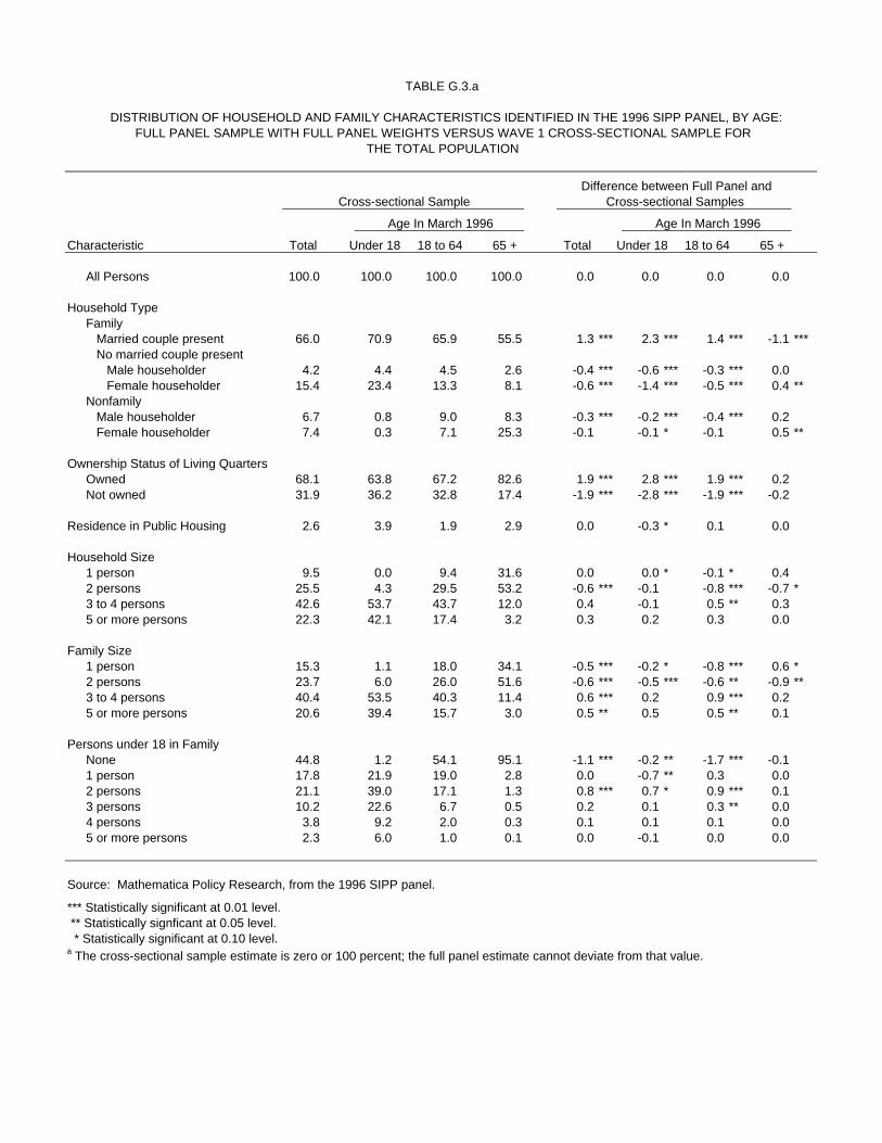
TABLE G.3.a

DISTRIBUTION OF HOUSEHOLD AND FAMILY CHARACTERISTICS IDENTIFIED IN THE 1996 SIPP PANEL, BY AGE:FULL PANEL SAMPLE WITH FULL PANEL WEIGHTS VERSUS WAVE 1 CROSS-SECTIONAL SAMPLE FOR

THE TOTAL POPULATION

Difference between Full Panel and Cross-sectional Sample Cross-sectional Samples

Age In March 1996 Age In March 1996

Characteristic Total Under 18 18 to 64 65 + Total Under 18 18 to 64 65 +

All Persons 100.0 100.0 100.0 100.0 0.0 0.0 0.0 0.0

Household TypeFamily Married couple present 66.0 70.9 65.9 55.5 1.3 *** 2.3 *** 1.4 *** -1.1 *** No married couple present Male householder 4.2 4.4 4.5 2.6 -0.4 *** -0.6 *** -0.3 *** 0.0 Female householder 15.4 23.4 13.3 8.1 -0.6 *** -1.4 *** -0.5 *** 0.4 **Nonfamily Male householder 6.7 0.8 9.0 8.3 -0.3 *** -0.2 *** -0.4 *** 0.2 Female householder 7.4 0.3 7.1 25.3 -0.1 -0.1 * -0.1 0.5 **

Ownership Status of Living QuartersOwned 68.1 63.8 67.2 82.6 1.9 *** 2.8 *** 1.9 *** 0.2 Not owned 31.9 36.2 32.8 17.4 -1.9 *** -2.8 *** -1.9 *** -0.2

Residence in Public Housing 2.6 3.9 1.9 2.9 0.0 -0.3 * 0.1 0.0

Household Size1 person 9.5 0.0 9.4 31.6 0.0 0.0 * -0.1 * 0.4 2 persons 25.5 4.3 29.5 53.2 -0.6 *** -0.1 -0.8 *** -0.7 *3 to 4 persons 42.6 53.7 43.7 12.0 0.4 -0.1 0.5 ** 0.3 5 or more persons 22.3 42.1 17.4 3.2 0.3 0.2 0.3 0.0

Family Size1 person 15.3 1.1 18.0 34.1 -0.5 *** -0.2 * -0.8 *** 0.6 *2 persons 23.7 6.0 26.0 51.6 -0.6 *** -0.5 *** -0.6 ** -0.9 **3 to 4 persons 40.4 53.5 40.3 11.4 0.6 *** 0.2 0.9 *** 0.2 5 or more persons 20.6 39.4 15.7 3.0 0.5 ** 0.5 0.5 ** 0.1

Persons under 18 in FamilyNone 44.8 1.2 54.1 95.1 -1.1 *** -0.2 ** -1.7 *** -0.1 1 person 17.8 21.9 19.0 2.8 0.0 -0.7 ** 0.3 0.0 2 persons 21.1 39.0 17.1 1.3 0.8 *** 0.7 * 0.9 *** 0.1 3 persons 10.2 22.6 6.7 0.5 0.2 0.1 0.3 ** 0.0 4 persons 3.8 9.2 2.0 0.3 0.1 0.1 0.1 0.0 5 or more persons 2.3 6.0 1.0 0.1 0.0 -0.1 0.0 0.0

Source: Mathematica Policy Research, from the 1996 SIPP panel.

*** Statistically significant at 0.01 level. ** Statistically signficant at 0.05 level. * Statistically significant at 0.10 level.a The cross-sectional sample estimate is zero or 100 percent; the full panel estimate cannot deviate from that value.

TABLE G.3.b

DISTRIBUTION OF HOUSEHOLD AND FAMILY CHARACTERISTICS IDENTIFIED IN THE 1996 SIPP PANEL, BY AGE:FULL PANEL SAMPLE WITH FULL PANEL WEIGHTS VERSUS WAVE 1 CROSS-SECTIONAL SAMPLE FOR

RETIRED WORKERS

Difference between Full Panel and Cross-sectional Sample Cross-sectional Samples

Age In March 1996 Age In March 1996

Characteristic Total Under 65 65 to 74 75 + Total Under 65 65 to 74 75 +

All Retired Workers 100.0 100.0 100.0 100.0 0.0 0.0 0.0 0.0

Household TypeFamily Married couple present 60.7 77.2 66.3 48.8 -1.2 *** -2.2 ** -1.4 ** -0.5 No married couple present Male householder 2.5 2.0 2.4 2.8 0.0 -0.4 0.0 0.2 Female householder 6.3 5.6 5.5 7.7 0.3 * 0.2 0.2 0.5 *Nonfamily Male householder 8.9 6.4 8.3 10.4 0.5 * 1.5 ** 0.4 0.2 Female householder 21.2 8.5 17.2 29.9 0.4 1.0 0.7 ** -0.4

Ownership Status of Living QuartersOwned 84.3 88.2 86.2 80.8 0.3 -0.3 0.1 0.7 Not owned 15.7 11.8 13.8 19.2 -0.3 0.3 -0.1 -0.7

Residence in Public Housing 2.6 1.9 2.0 3.5 0.1 0.2 0.1 0.1

Household Size1 person 28.3 12.7 23.3 39.1 0.5 1.7 ** 1.1 ** -0.6 2 persons 57.7 68.8 62.0 49.0 -0.7 * -0.9 -1.1 ** 0.0 3 to 4 persons 11.6 14.9 12.4 9.5 0.2 -0.2 0.2 0.5 5 or more persons 2.5 3.7 2.3 2.3 -0.1 -0.5 -0.1 0.1

Family Size1 person 30.5 15.2 25.9 40.7 0.8 ** 2.2 ** 1.2 ** -0.1 2 persons 56.1 67.0 60.1 47.9 -0.9 ** -1.2 -1.3 ** -0.2 3 to 4 persons 11.1 14.5 11.8 9.1 0.1 -0.2 0.2 0.1 5 or more persons 2.3 3.4 2.1 2.2 -0.1 -0.8 * -0.1 0.2

Persons under 18 in FamilyNone 95.7 92.0 95.5 97.0 0.1 1.1 0.1 -0.2 1 person 2.6 5.1 2.8 1.5 -0.1 -1.0 * -0.1 0.1 2 persons 1.0 1.9 0.8 0.9 0.0 -0.3 0.0 0.0 3 persons 0.5 0.6 0.5 0.4 0.1 0.2 0.0 0.1 4 persons 0.2 0.4 0.3 0.1 0.0 0.0 0.0 0.0 5 or more persons 0.0 0.0 0.0 0.1 0.0 0.0 a 0.0 0.0

Source: Mathematica Policy Research, from the 1996 SIPP panel.

*** Statistically significant at 0.01 level. ** Statistically signficant at 0.05 level. * Statistically significant at 0.10 level.a The cross-sectional sample estimate is zero or 100 percent; the full panel estimate cannot deviate from that value.

TABLE G.3.c

DISTRIBUTION OF HOUSEHOLD AND FAMILY CHARACTERISTICS IDENTIFIED IN THE 1996 SIPP PANEL, BY AGE:FULL PANEL SAMPLE WITH FULL PANEL WEIGHTS VERSUS WAVE 1 CROSS-SECTIONAL SAMPLE FOR

DISABLED WORKERS

Difference between Full Panel and Cross-sectional Sample Cross-sectional Samples

Age In March 1996 Age In March 1996

Characteristic Total Under 50 50 to 64 65 + Total Under 50 50 to 64 65 +

All Disabled Workers 100.0 100.0 100.0 100.0 0.0 0.0 0.0 0.0

Household TypeFamily Married couple present 48.9 43.0 54.3 48.1 1.6 * 1.5 1.0 3.5 ** No married couple present Male householder 5.8 8.3 4.8 4.0 0.3 -0.5 0.5 0.8 Female householder 15.7 21.9 12.2 13.0 -0.1 1.1 -0.7 -1.7 Nonfamily Male householder 13.5 16.0 13.1 10.8 -0.9 -1.5 -0.4 -1.0 Female householder 15.4 9.6 15.3 23.0 -1.1 -0.6 -0.4 -1.9

Ownership Status of Living QuartersOwned 64.4 51.8 70.9 70.4 0.6 3.2 * -0.1 -0.2 Not owned 35.6 48.2 29.1 29.6 -0.6 -3.2 * 0.1 0.2

Residence in Public Housing 6.9 7.6 5.9 7.6 0.3 0.7 0.6 -0.8

Household Size1 person 23.4 19.2 22.5 30.0 -1.2 * -0.9 0.5 -3.7 ***2 persons 38.5 24.6 48.5 40.9 0.3 0.9 -1.3 3.6 **3 to 4 persons 27.8 40.9 21.4 20.9 0.6 -0.8 0.7 0.4 5 or more persons 10.3 15.3 7.5 8.2 0.4 0.7 0.1 -0.4

Family Size1 person 31.4 30.6 28.8 36.4 -2.1 ** -2.8 -0.8 -3.1 **2 persons 34.8 20.6 44.3 38.2 0.8 1.4 0.1 3.1 **3 to 4 persons 25.3 37.1 19.9 18.4 0.6 -0.4 0.7 0.0 5 or more persons 8.6 11.7 7.0 7.0 0.7 1.7 0.0 0.0

Persons under 18 in FamilyNone 80.6 66.8 86.0 90.0 -0.4 -0.1 0.3 0.1 1 person 9.5 16.3 7.1 4.7 -0.4 -0.7 -0.8 -0.3 2 persons 5.5 10.7 3.4 2.3 0.3 -0.2 -0.1 0.7 3 persons 2.6 3.7 2.2 1.7 0.2 0.8 0.3 -0.8 4 persons 1.2 1.6 1.1 1.0 0.1 0.0 0.4 0.0 5 or more persons 0.5 0.9 0.2 0.4 0.1 0.2 -0.1 0.2

Source: Mathematica Policy Research, from the 1996 SIPP panel.

*** Statistically significant at 0.01 level. ** Statistically signficant at 0.05 level. * Statistically significant at 0.10 level.a The cross-sectional sample estimate is zero or 100 percent; the full panel estimate cannot deviate from that value.

TABLE G.3.d

DISTRIBUTION OF HOUSEHOLD AND FAMILY CHARACTERISTICS IDENTIFIED IN THE 1996 SIPP PANEL, BY AGE:FULL PANEL SAMPLE WITH FULL PANEL WEIGHTS VERSUS WAVE 1 CROSS-SECTIONAL SAMPLE FOR

ALL OTHER SOCIAL SECURITY BENEFICIARIES

Difference between Full Panel and Cross-sectional Sample Cross-sectional Samples

Age In March 1996 Age In March 1996

Characteristic Total Under 18 18 to 64 65 + Total Under 18 18 to 64 65 +

All Other Beneficiaries 100.0 100.0 100.0 100.0 0.0 0.0 0.0 0.0

Household TypeFamily Married couple present 36.4 44.1 36.3 33.7 -1.2 * -0.8 0.9 -2.1 *** No married couple present Male householder 2.8 6.3 3.3 1.4 -0.4 -1.1 -0.3 -0.2 Female householder 24.5 48.2 32.6 13.8 2.4 *** 1.9 3.4 ** 1.3 **Nonfamily Male householder 2.0 1.0 5.1 1.6 -0.4 * -0.1 -2.1 *** 0.0 Female householder 34.0 0.1 22.6 49.4 -0.3 0.1 -1.8 1.2

Ownership Status of Living QuartersOwned 75.9 62.8 71.8 81.8 0.6 0.7 1.6 0.9 Not owned 24.1 37.2 28.2 18.2 -0.6 -0.7 -1.6 -0.9

Residence in Public Housing 4.3 6.1 4.6 3.5 -0.2 0.2 -0.8 -0.2

Household Size1 person 34.4 0.0 23.0 49.9 -0.7 0.0 a -2.3 * 0.7 2 persons 29.4 10.1 29.8 36.5 -0.7 1.7 * -1.6 -0.9 3 to 4 persons 24.5 54.9 34.7 10.7 0.4 -4.0 ** 2.4 0.4 5 or more persons 11.7 35.0 12.4 2.9 1.1 2.3 1.5 -0.3

Family Size1 person 36.5 1.4 29.0 51.4 -0.5 0.7 -3.5 ** 1.1 2 persons 28.9 11.9 27.2 35.6 -0.8 0.5 0.4 -1.1 3 to 4 persons 24.1 55.6 32.7 10.3 0.9 -1.9 2.6 0.3 5 or more persons 10.5 31.1 11.1 2.7 0.5 0.7 0.5 -0.3

Persons under 18 in FamilyNone 68.7 1.4 63.7 94.9 -1.5 ** 0.7 -2.5 0.1 1 person 11.7 30.2 19.4 3.0 0.5 -0.2 1.2 -0.2 2 persons 9.8 33.1 9.6 1.3 0.3 -1.2 -0.5 0.3 *3 persons 5.6 19.4 4.8 0.6 -0.2 -1.8 0.4 -0.2 4 persons 2.4 9.0 1.6 0.2 0.5 1.1 0.8 * 0.0 5 or more persons 1.7 7.0 0.8 0.0 0.5 * 1.3 0.6 * 0.0

Source: Mathematica Policy Research, from the 1996 SIPP panel.

*** Statistically significant at 0.01 level. ** Statistically signficant at 0.05 level. * Statistically significant at 0.10 level.a The cross-sectional sample estimate is zero or 100 percent; the full panel estimate cannot deviate from that value.

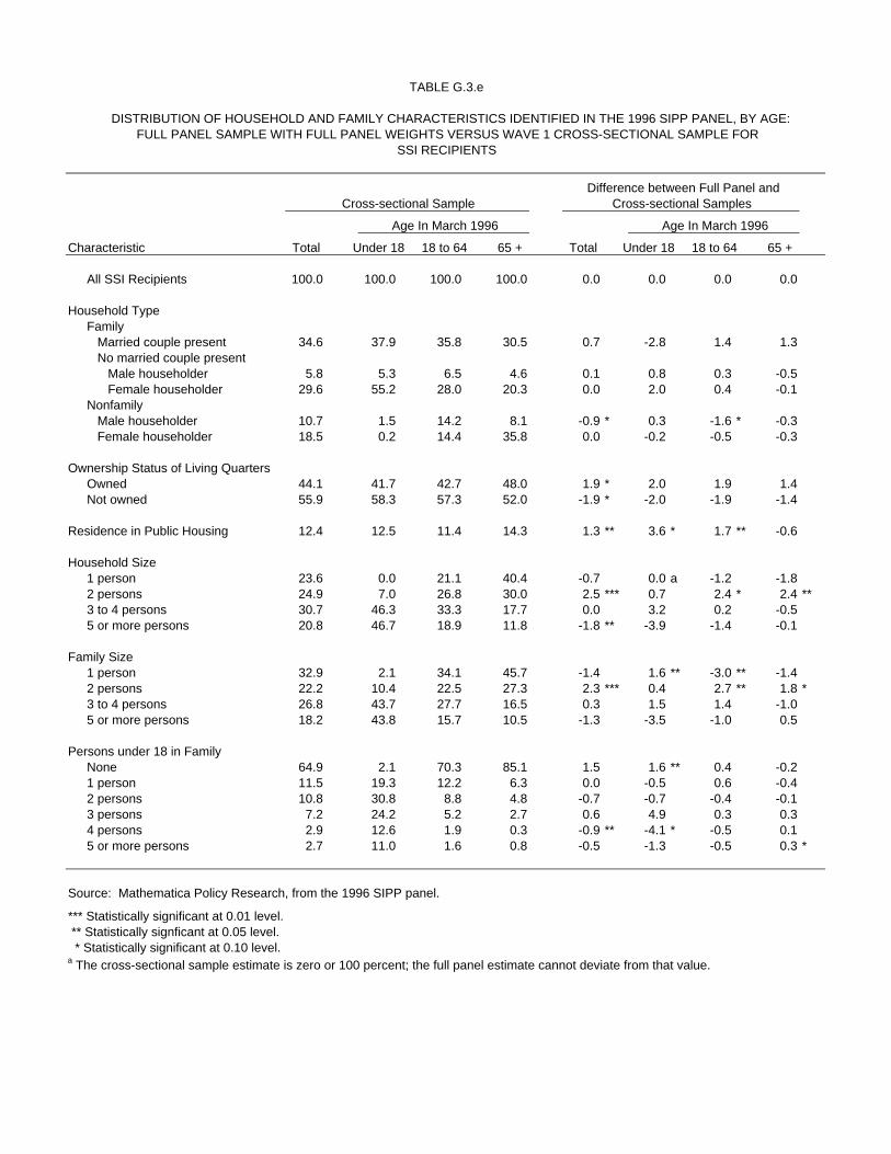
TABLE G.3.e

DISTRIBUTION OF HOUSEHOLD AND FAMILY CHARACTERISTICS IDENTIFIED IN THE 1996 SIPP PANEL, BY AGE:FULL PANEL SAMPLE WITH FULL PANEL WEIGHTS VERSUS WAVE 1 CROSS-SECTIONAL SAMPLE FOR

SSI RECIPIENTS

Difference between Full Panel and Cross-sectional Sample Cross-sectional Samples

Age In March 1996 Age In March 1996

Characteristic Total Under 18 18 to 64 65 + Total Under 18 18 to 64 65 +

All SSI Recipients 100.0 100.0 100.0 100.0 0.0 0.0 0.0 0.0

Household TypeFamily Married couple present 34.6 37.9 35.8 30.5 0.7 -2.8 1.4 1.3 No married couple present Male householder 5.8 5.3 6.5 4.6 0.1 0.8 0.3 -0.5 Female householder 29.6 55.2 28.0 20.3 0.0 2.0 0.4 -0.1 Nonfamily Male householder 10.7 1.5 14.2 8.1 -0.9 * 0.3 -1.6 * -0.3 Female householder 18.5 0.2 14.4 35.8 0.0 -0.2 -0.5 -0.3

Ownership Status of Living QuartersOwned 44.1 41.7 42.7 48.0 1.9 * 2.0 1.9 1.4 Not owned 55.9 58.3 57.3 52.0 -1.9 * -2.0 -1.9 -1.4

Residence in Public Housing 12.4 12.5 11.4 14.3 1.3 ** 3.6 * 1.7 ** -0.6

Household Size1 person 23.6 0.0 21.1 40.4 -0.7 0.0 a -1.2 -1.8 2 persons 24.9 7.0 26.8 30.0 2.5 *** 0.7 2.4 * 2.4 **3 to 4 persons 30.7 46.3 33.3 17.7 0.0 3.2 0.2 -0.5 5 or more persons 20.8 46.7 18.9 11.8 -1.8 ** -3.9 -1.4 -0.1

Family Size1 person 32.9 2.1 34.1 45.7 -1.4 1.6 ** -3.0 ** -1.4 2 persons 22.2 10.4 22.5 27.3 2.3 *** 0.4 2.7 ** 1.8 *3 to 4 persons 26.8 43.7 27.7 16.5 0.3 1.5 1.4 -1.0 5 or more persons 18.2 43.8 15.7 10.5 -1.3 -3.5 -1.0 0.5

Persons under 18 in FamilyNone 64.9 2.1 70.3 85.1 1.5 1.6 ** 0.4 -0.2 1 person 11.5 19.3 12.2 6.3 0.0 -0.5 0.6 -0.4 2 persons 10.8 30.8 8.8 4.8 -0.7 -0.7 -0.4 -0.1 3 persons 7.2 24.2 5.2 2.7 0.6 4.9 0.3 0.3 4 persons 2.9 12.6 1.9 0.3 -0.9 ** -4.1 * -0.5 0.1 5 or more persons 2.7 11.0 1.6 0.8 -0.5 -1.3 -0.5 0.3 *

Source: Mathematica Policy Research, from the 1996 SIPP panel.

*** Statistically significant at 0.01 level. ** Statistically signficant at 0.05 level. * Statistically significant at 0.10 level.a The cross-sectional sample estimate is zero or 100 percent; the full panel estimate cannot deviate from that value.

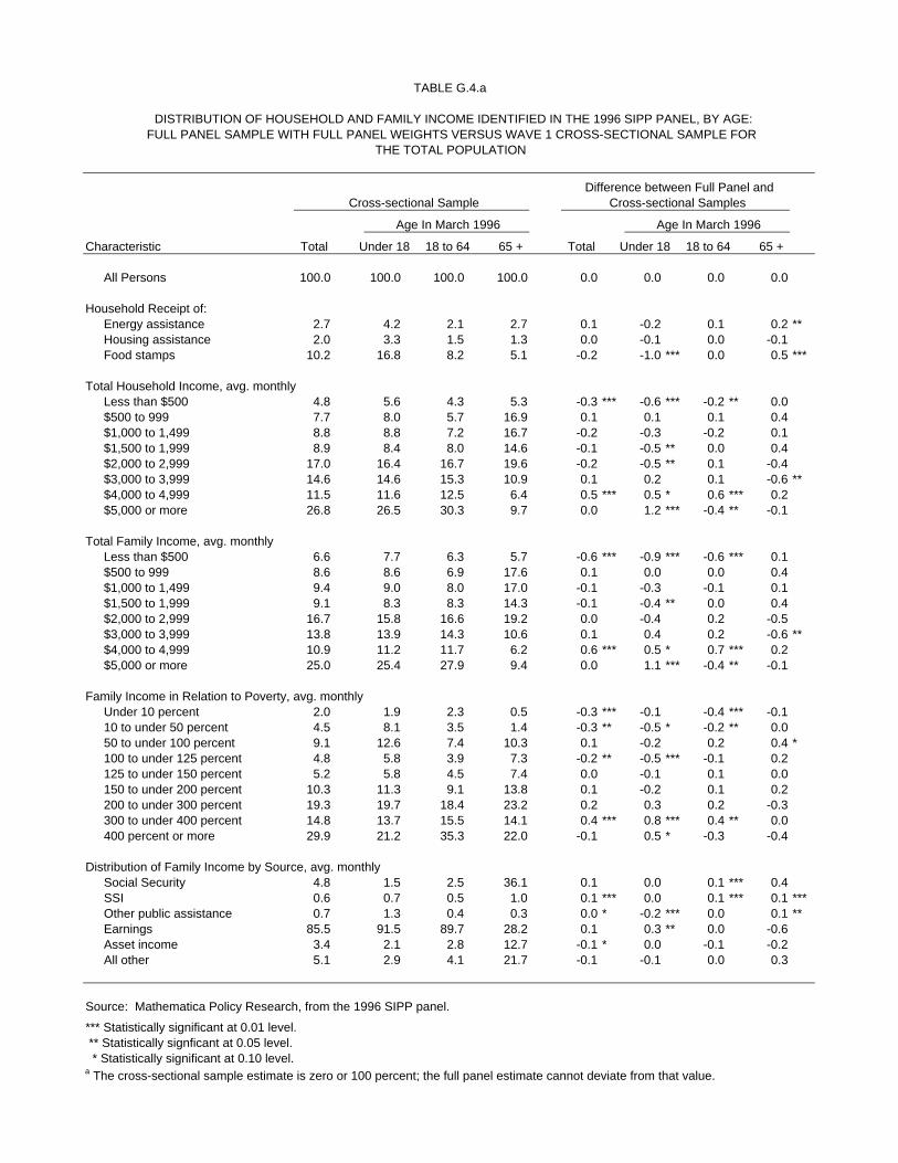
TABLE G.4.a

DISTRIBUTION OF HOUSEHOLD AND FAMILY INCOME IDENTIFIED IN THE 1996 SIPP PANEL, BY AGE:FULL PANEL SAMPLE WITH FULL PANEL WEIGHTS VERSUS WAVE 1 CROSS-SECTIONAL SAMPLE FOR

THE TOTAL POPULATION

Difference between Full Panel and Cross-sectional Sample Cross-sectional Samples

Age In March 1996 Age In March 1996

Characteristic Total Under 18 18 to 64 65 + Total Under 18 18 to 64 65 +

All Persons 100.0 100.0 100.0 100.0 0.0 0.0 0.0 0.0

Household Receipt of:Energy assistance 2.7 4.2 2.1 2.7 0.1 -0.2 0.1 0.2 **Housing assistance 2.0 3.3 1.5 1.3 0.0 -0.1 0.0 -0.1 Food stamps 10.2 16.8 8.2 5.1 -0.2 -1.0 *** 0.0 0.5 ***

Total Household Income, avg. monthlyLess than $500 4.8 5.6 4.3 5.3 -0.3 *** -0.6 *** -0.2 ** 0.0 $500 to 999 7.7 8.0 5.7 16.9 0.1 0.1 0.1 0.4 $1,000 to 1,499 8.8 8.8 7.2 16.7 -0.2 -0.3 -0.2 0.1 $1,500 to 1,999 8.9 8.4 8.0 14.6 -0.1 -0.5 ** 0.0 0.4 $2,000 to 2,999 17.0 16.4 16.7 19.6 -0.2 -0.5 ** 0.1 -0.4 $3,000 to 3,999 14.6 14.6 15.3 10.9 0.1 0.2 0.1 -0.6 **$4,000 to 4,999 11.5 11.6 12.5 6.4 0.5 *** 0.5 * 0.6 *** 0.2 $5,000 or more 26.8 26.5 30.3 9.7 0.0 1.2 *** -0.4 ** -0.1

Total Family Income, avg. monthlyLess than $500 6.6 7.7 6.3 5.7 -0.6 *** -0.9 *** -0.6 *** 0.1 $500 to 999 8.6 8.6 6.9 17.6 0.1 0.0 0.0 0.4 $1,000 to 1,499 9.4 9.0 8.0 17.0 -0.1 -0.3 -0.1 0.1 $1,500 to 1,999 9.1 8.3 8.3 14.3 -0.1 -0.4 ** 0.0 0.4 $2,000 to 2,999 16.7 15.8 16.6 19.2 0.0 -0.4 0.2 -0.5 $3,000 to 3,999 13.8 13.9 14.3 10.6 0.1 0.4 0.2 -0.6 **$4,000 to 4,999 10.9 11.2 11.7 6.2 0.6 *** 0.5 * 0.7 *** 0.2 $5,000 or more 25.0 25.4 27.9 9.4 0.0 1.1 *** -0.4 ** -0.1

Family Income in Relation to Poverty, avg. monthlyUnder 10 percent 2.0 1.9 2.3 0.5 -0.3 *** -0.1 -0.4 *** -0.1 10 to under 50 percent 4.5 8.1 3.5 1.4 -0.3 ** -0.5 * -0.2 ** 0.0 50 to under 100 percent 9.1 12.6 7.4 10.3 0.1 -0.2 0.2 0.4 *100 to under 125 percent 4.8 5.8 3.9 7.3 -0.2 ** -0.5 *** -0.1 0.2 125 to under 150 percent 5.2 5.8 4.5 7.4 0.0 -0.1 0.1 0.0 150 to under 200 percent 10.3 11.3 9.1 13.8 0.1 -0.2 0.1 0.2 200 to under 300 percent 19.3 19.7 18.4 23.2 0.2 0.3 0.2 -0.3 300 to under 400 percent 14.8 13.7 15.5 14.1 0.4 *** 0.8 *** 0.4 ** 0.0 400 percent or more 29.9 21.2 35.3 22.0 -0.1 0.5 * -0.3 -0.4

Distribution of Family Income by Source, avg. monthlySocial Security 4.8 1.5 2.5 36.1 0.1 0.0 0.1 *** 0.4 SSI 0.6 0.7 0.5 1.0 0.1 *** 0.0 0.1 *** 0.1 ***Other public assistance 0.7 1.3 0.4 0.3 0.0 * -0.2 *** 0.0 0.1 **Earnings 85.5 91.5 89.7 28.2 0.1 0.3 ** 0.0 -0.6 Asset income 3.4 2.1 2.8 12.7 -0.1 * 0.0 -0.1 -0.2 All other 5.1 2.9 4.1 21.7 -0.1 -0.1 0.0 0.3

Source: Mathematica Policy Research, from the 1996 SIPP panel.

*** Statistically significant at 0.01 level. ** Statistically signficant at 0.05 level. * Statistically significant at 0.10 level.a The cross-sectional sample estimate is zero or 100 percent; the full panel estimate cannot deviate from that value.

TABLE G.4.b

DISTRIBUTION OF HOUSEHOLD AND FAMILY INCOME IDENTIFIED IN THE 1996 SIPP PANEL, BY AGE:FULL PANEL SAMPLE WITH FULL PANEL WEIGHTS VERSUS WAVE 1 CROSS-SECTIONAL SAMPLE FOR

RETIRED WORKERS

Difference between Full Panel and Cross-sectional Sample Cross-sectional Samples

Age In March 1996 Age In March 1996

Characteristic Total Under 65 65 to 74 75 + Total Under 65 65 to 74 75 +

All Retired Workers 100.0 100.0 100.0 100.0 0.0 0.0 0.0 0.0

Household Receipt of:Energy assistance 2.4 1.6 2.1 3.0 0.2 * -0.1 0.1 0.4 *Housing assistance 1.2 0.5 1.2 1.3 -0.1 0.1 0.0 -0.1 Food stamps 3.6 3.9 4.0 3.1 0.3 ** 0.8 0.1 0.3

Total Household Income, avg. monthlyLess than $500 3.9 2.9 3.1 5.3 0.1 0.0 0.0 0.3 $500 to 999 15.3 7.5 12.6 21.1 0.2 1.1 * 0.5 -0.6 $1,000 to 1,499 16.9 14.6 16.4 18.3 0.0 -0.4 0.5 -0.4 $1,500 to 1,999 15.0 12.5 15.1 15.7 0.5 * 0.4 0.2 1.0 **$2,000 to 2,999 21.2 24.8 22.7 18.2 -0.4 0.6 -0.4 -0.7 $3,000 to 3,999 11.6 13.6 13.3 8.7 -0.4 -1.0 -0.2 -0.5 $4,000 to 4,999 6.9 10.9 7.1 5.6 0.2 -0.2 0.1 0.5 $5,000 or more 9.1 13.4 9.7 7.2 -0.2 -0.6 -0.6 * 0.4

Total Family Income, avg. monthlyLess than $500 4.2 3.0 3.5 5.4 0.2 0.1 0.1 0.3 $500 to 999 16.0 8.0 13.3 21.6 0.3 1.2 * 0.6 -0.4 $1,000 to 1,499 17.2 14.8 16.6 18.7 0.0 -0.2 0.4 -0.3 $1,500 to 1,999 14.9 12.7 14.9 15.4 0.4 0.2 0.2 0.9 *$2,000 to 2,999 21.0 25.0 22.4 18.0 -0.4 0.7 -0.4 -0.7 $3,000 to 3,999 11.3 13.5 13.2 8.3 -0.5 * -1.0 -0.2 -0.6 *$4,000 to 4,999 6.7 10.2 6.8 5.5 0.2 -0.3 0.1 0.5 $5,000 or more 8.8 12.8 9.4 7.0 -0.3 -0.7 -0.7 ** 0.4

Family Income in Relation to Poverty, avg. monthlyUnder 10 percent 0.1 0.1 0.1 0.1 0.0 0.0 0.0 0.0 10 to under 50 percent 1.1 1.2 0.9 1.3 0.0 0.1 0.2 -0.1 50 to under 100 percent 8.7 6.8 7.7 10.7 0.3 0.6 0.1 0.3 100 to under 125 percent 6.6 3.6 6.0 8.1 0.2 0.0 0.4 -0.1 125 to under 150 percent 7.5 7.2 5.9 9.6 0.1 1.2 0.1 -0.2 150 to under 200 percent 14.1 11.5 13.5 15.5 -0.1 -2.1 ** 0.1 0.2 200 to under 300 percent 24.5 24.6 25.1 23.7 0.2 2.9 ** 0.2 -0.5 300 to under 400 percent 15.2 17.7 16.2 13.1 -0.3 -1.5 -0.8 * 0.5 400 percent or more 22.4 27.2 24.8 17.9 -0.3 -1.1 -0.3 -0.1

Distribution of Family Income by Source, avg. monthlySocial Security 39.2 31.1 37.7 44.8 0.2 1.1 0.2 -0.4 SSI 0.5 0.4 0.5 0.5 0.0 * 0.1 0.1 0.0 Other public assistance 0.3 0.3 0.2 0.3 0.1 *** 0.1 0.0 0.1 ***Earnings 24.1 32.2 25.3 19.1 0.0 -2.1 0.0 1.1 *Asset income 12.8 10.0 12.1 14.9 -0.5 * -0.2 -0.7 ** -0.5 All other 23.2 26.1 24.2 20.4 0.2 1.0 0.4 -0.3

Source: Mathematica Policy Research, from the 1996 SIPP panel.

*** Statistically significant at 0.01 level. ** Statistically signficant at 0.05 level. * Statistically significant at 0.10 level.a The cross-sectional sample estimate is zero or 100 percent; the full panel estimate cannot deviate from that value.

TABLE G.4.c

DISTRIBUTION OF HOUSEHOLD AND FAMILY INCOME IDENTIFIED IN THE 1996 SIPP PANEL, BY AGE:FULL PANEL SAMPLE WITH FULL PANEL WEIGHTS VERSUS WAVE 1 CROSS-SECTIONAL SAMPLE FOR

DISABLED WORKERS

Difference between Full Panel and Cross-sectional Sample Cross-sectional Samples

Age In March 1996 Age In March 1996

Characteristic Total Under 50 50 to 64 65 + Total Under 50 50 to 64 65 +

All Disabled Workers 100.0 100.0 100.0 100.0 0.0 0.0 0.0 0.0

Household Receipt of:Energy assistance 6.8 7.5 6.2 6.9 1.1 ** 1.9 ** 0.9 0.0 Housing assistance 4.0 5.8 2.6 4.0 -0.3 -0.1 0.0 -1.3 *Food stamps 20.5 27.5 15.3 19.4 1.2 * 0.0 2.0 * 0.7

Total Household Income, avg. monthlyLess than $500 6.9 4.9 6.5 10.3 0.7 1.1 0.6 0.3 $500 to 999 20.7 20.0 18.5 25.0 -0.6 -0.6 0.7 -2.5 *$1,000 to 1,499 16.8 16.1 16.8 17.5 0.8 0.1 1.0 1.6 $1,500 to 1,999 13.9 12.9 13.2 16.1 -0.3 -1.5 -1.3 2.9 **$2,000 to 2,999 16.8 19.4 17.4 12.7 -0.3 0.0 -0.2 -1.0 $3,000 to 3,999 11.0 11.8 12.5 7.7 -0.5 0.1 -0.4 -1.6 $4,000 to 4,999 6.0 4.6 7.8 4.8 -0.2 0.2 -0.8 0.2 $5,000 or more 7.9 10.3 7.3 6.0 0.4 0.5 0.4 0.0

Total Family Income, avg. monthlyLess than $500 8.8 8.4 7.2 11.9 0.4 0.0 0.7 0.7 $500 to 999 24.3 24.6 21.5 28.4 -1.0 -1.0 -0.1 -2.4 *$1,000 to 1,499 15.8 15.2 16.0 16.3 1.0 * 0.4 1.0 1.8 $1,500 to 1,999 12.6 10.7 12.8 14.9 0.1 -0.5 -0.6 2.3 *$2,000 to 2,999 15.8 18.6 16.4 11.4 -0.6 -0.1 -0.8 -1.4 $3,000 to 3,999 9.9 10.5 11.5 6.7 -0.3 0.1 -0.1 -1.2 $4,000 to 4,999 5.5 3.6 7.5 4.8 0.0 0.8 * -0.6 0.2 $5,000 or more 7.2 8.5 7.1 5.7 0.3 0.3 0.5 0.0

Family Income in Relation to Poverty, avg. monthlyUnder 10 percent 0.1 0.2 0.0 0.0 -0.1 -0.2 0.0 a 0.0 a10 to under 50 percent 2.4 1.7 2.5 3.2 0.1 -0.2 0.5 -0.1 50 to under 100 percent 21.8 27.4 16.4 23.0 0.6 -0.6 1.6 -0.1 100 to under 125 percent 10.7 9.8 10.5 12.3 -0.7 -0.2 -0.7 -1.3 125 to under 150 percent 9.3 9.0 9.1 10.0 0.8 * 1.2 0.2 1.3 150 to under 200 percent 14.6 13.5 14.4 16.2 0.0 -0.6 -0.6 1.8 *200 to under 300 percent 19.3 19.4 20.7 17.0 0.4 1.1 -0.3 0.6 300 to under 400 percent 11.0 10.9 11.8 10.0 -0.9 * -0.4 -0.7 -1.9 **400 percent or more 10.8 8.2 14.5 8.4 -0.2 -0.1 0.1 -0.3

Distribution of Family Income by Source, avg. monthlySocial Security 38.3 36.5 37.0 43.5 0.6 0.0 1.0 1.0 SSI 3.5 4.6 2.2 4.1 0.1 -0.4 0.4 0.3 Other public assistance 1.2 1.2 1.0 1.6 0.0 0.1 -0.2 0.0 Earnings 39.4 44.7 40.3 29.5 -0.8 -0.8 -0.7 -1.6 Asset income 3.6 2.4 3.4 5.9 0.3 0.1 0.4 * 0.8 All other 14.1 10.6 16.2 15.3 -0.2 1.0 -0.8 -0.4

Source: Mathematica Policy Research, from the 1996 SIPP panel.

*** Statistically significant at 0.01 level. ** Statistically signficant at 0.05 level. * Statistically significant at 0.10 level.a The cross-sectional sample estimate is zero or 100 percent; the full panel estimate cannot deviate from that value.

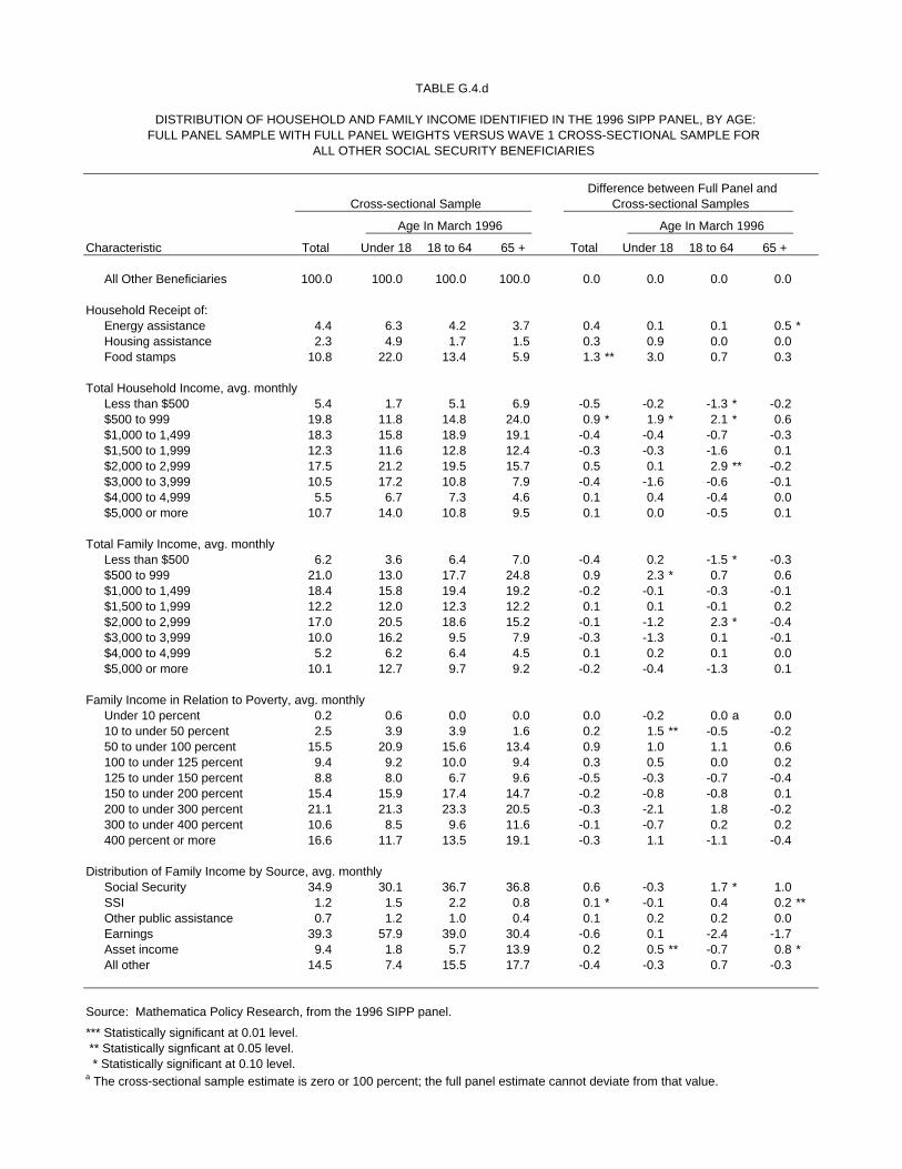
TABLE G.4.d

DISTRIBUTION OF HOUSEHOLD AND FAMILY INCOME IDENTIFIED IN THE 1996 SIPP PANEL, BY AGE:FULL PANEL SAMPLE WITH FULL PANEL WEIGHTS VERSUS WAVE 1 CROSS-SECTIONAL SAMPLE FOR

ALL OTHER SOCIAL SECURITY BENEFICIARIES

Difference between Full Panel and Cross-sectional Sample Cross-sectional Samples

Age In March 1996 Age In March 1996

Characteristic Total Under 18 18 to 64 65 + Total Under 18 18 to 64 65 +

All Other Beneficiaries 100.0 100.0 100.0 100.0 0.0 0.0 0.0 0.0

Household Receipt of:Energy assistance 4.4 6.3 4.2 3.7 0.4 0.1 0.1 0.5 *Housing assistance 2.3 4.9 1.7 1.5 0.3 0.9 0.0 0.0 Food stamps 10.8 22.0 13.4 5.9 1.3 ** 3.0 0.7 0.3

Total Household Income, avg. monthlyLess than $500 5.4 1.7 5.1 6.9 -0.5 -0.2 -1.3 * -0.2 $500 to 999 19.8 11.8 14.8 24.0 0.9 * 1.9 * 2.1 * 0.6 $1,000 to 1,499 18.3 15.8 18.9 19.1 -0.4 -0.4 -0.7 -0.3 $1,500 to 1,999 12.3 11.6 12.8 12.4 -0.3 -0.3 -1.6 0.1 $2,000 to 2,999 17.5 21.2 19.5 15.7 0.5 0.1 2.9 ** -0.2 $3,000 to 3,999 10.5 17.2 10.8 7.9 -0.4 -1.6 -0.6 -0.1 $4,000 to 4,999 5.5 6.7 7.3 4.6 0.1 0.4 -0.4 0.0 $5,000 or more 10.7 14.0 10.8 9.5 0.1 0.0 -0.5 0.1

Total Family Income, avg. monthlyLess than $500 6.2 3.6 6.4 7.0 -0.4 0.2 -1.5 * -0.3 $500 to 999 21.0 13.0 17.7 24.8 0.9 2.3 * 0.7 0.6 $1,000 to 1,499 18.4 15.8 19.4 19.2 -0.2 -0.1 -0.3 -0.1 $1,500 to 1,999 12.2 12.0 12.3 12.2 0.1 0.1 -0.1 0.2 $2,000 to 2,999 17.0 20.5 18.6 15.2 -0.1 -1.2 2.3 * -0.4 $3,000 to 3,999 10.0 16.2 9.5 7.9 -0.3 -1.3 0.1 -0.1 $4,000 to 4,999 5.2 6.2 6.4 4.5 0.1 0.2 0.1 0.0 $5,000 or more 10.1 12.7 9.7 9.2 -0.2 -0.4 -1.3 0.1

Family Income in Relation to Poverty, avg. monthlyUnder 10 percent 0.2 0.6 0.0 0.0 0.0 -0.2 0.0 a 0.0 10 to under 50 percent 2.5 3.9 3.9 1.6 0.2 1.5 ** -0.5 -0.2 50 to under 100 percent 15.5 20.9 15.6 13.4 0.9 1.0 1.1 0.6 100 to under 125 percent 9.4 9.2 10.0 9.4 0.3 0.5 0.0 0.2 125 to under 150 percent 8.8 8.0 6.7 9.6 -0.5 -0.3 -0.7 -0.4 150 to under 200 percent 15.4 15.9 17.4 14.7 -0.2 -0.8 -0.8 0.1 200 to under 300 percent 21.1 21.3 23.3 20.5 -0.3 -2.1 1.8 -0.2 300 to under 400 percent 10.6 8.5 9.6 11.6 -0.1 -0.7 0.2 0.2 400 percent or more 16.6 11.7 13.5 19.1 -0.3 1.1 -1.1 -0.4

Distribution of Family Income by Source, avg. monthlySocial Security 34.9 30.1 36.7 36.8 0.6 -0.3 1.7 * 1.0 SSI 1.2 1.5 2.2 0.8 0.1 * -0.1 0.4 0.2 **Other public assistance 0.7 1.2 1.0 0.4 0.1 0.2 0.2 0.0 Earnings 39.3 57.9 39.0 30.4 -0.6 0.1 -2.4 -1.7 Asset income 9.4 1.8 5.7 13.9 0.2 0.5 ** -0.7 0.8 *All other 14.5 7.4 15.5 17.7 -0.4 -0.3 0.7 -0.3

Source: Mathematica Policy Research, from the 1996 SIPP panel.

*** Statistically significant at 0.01 level. ** Statistically signficant at 0.05 level. * Statistically significant at 0.10 level.a The cross-sectional sample estimate is zero or 100 percent; the full panel estimate cannot deviate from that value.

TABLE G.4.e

DISTRIBUTION OF HOUSEHOLD AND FAMILY INCOME IDENTIFIED IN THE 1996 SIPP PANEL, BY AGE:FULL PANEL SAMPLE WITH FULL PANEL WEIGHTS VERSUS WAVE 1 CROSS-SECTIONAL SAMPLE FOR

SSI RECIPIENTS

Difference between Full Panel and Cross-sectional Sample Cross-sectional Samples

Age In March 1996 Age In March 1996

Characteristic Total Under 18 18 to 64 65 + Total Under 18 18 to 64 65 +

All SSI Recipients 100.0 100.0 100.0 100.0 0.0 0.0 0.0 0.0

Household Receipt of:Energy assistance 12.7 13.3 12.3 13.2 -0.1 -2.2 0.1 0.4 Housing assistance 8.9 12.9 8.5 7.6 -0.5 -2.8 -0.1 0.1 Food stamps 45.0 41.2 47.0 42.8 0.0 -2.9 0.2 0.8

Total Household Income, avg. monthlyLess than $500 15.4 2.4 13.7 25.4 1.0 0.4 1.3 -0.2 $500 to 999 25.9 18.6 25.0 31.3 -0.8 -1.6 -1.1 -0.3 $1,000 to 1,499 17.4 25.5 15.5 17.2 1.3 * 3.7 0.9 1.5 $1,500 to 1,999 10.8 17.2 11.4 6.3 -0.4 1.5 -0.7 0.0 $2,000 to 2,999 13.6 17.9 15.8 7.1 -0.9 -1.6 -0.7 -0.6 $3,000 to 3,999 6.2 10.4 6.7 2.9 -0.4 0.1 -0.2 -0.6 $4,000 to 4,999 4.4 4.4 4.2 4.6 -0.3 -0.7 -0.2 -0.5 $5,000 or more 6.4 3.7 7.6 5.1 0.5 -1.8 0.7 0.8

Total Family Income, avg. monthlyLess than $500 20.3 5.8 20.0 27.9 0.6 2.0 0.2 0.0 $500 to 999 28.4 20.8 27.6 33.8 -0.8 -3.4 -0.9 0.0 $1,000 to 1,499 16.0 24.4 14.5 14.8 1.5 ** 3.8 1.2 1.7 $1,500 to 1,999 9.0 17.3 8.9 5.0 -0.3 0.4 -0.3 -0.3 $2,000 to 2,999 12.3 16.6 13.8 6.9 -0.5 -1.6 0.1 -0.8 $3,000 to 3,999 5.1 8.3 5.5 2.7 -0.2 0.5 -0.1 -0.4 $4,000 to 4,999 3.9 4.4 3.8 3.8 -0.4 -0.6 -0.1 -0.8 $5,000 or more 5.0 2.4 5.7 5.0 0.0 -1.1 -0.1 0.7

Family Income in Relation to Poverty, avg. monthlyUnder 10 percent 0.3 0.4 0.3 0.3 0.0 -0.1 0.0 0.1 10 to under 50 percent 3.9 6.6 3.6 3.1 0.2 0.2 0.2 0.4 50 to under 100 percent 42.5 35.1 42.3 46.4 -0.9 -3.2 -0.5 -1.3 100 to under 125 percent 12.8 16.3 10.7 15.6 0.3 2.6 -0.6 1.2 125 to under 150 percent 9.6 11.7 9.0 10.0 1.1 * -0.5 1.4 * 1.1 150 to under 200 percent 10.8 14.8 11.6 7.3 0.6 4.7 * -0.2 0.5 200 to under 300 percent 10.6 9.1 11.4 9.7 -0.5 -0.9 0.4 -2.2 **300 to under 400 percent 4.9 4.7 5.5 3.9 0.0 -1.6 0.1 0.4 400 percent or more 4.4 1.2 5.6 3.6 -0.7 * -1.2 ** -0.8 -0.2

Distribution of Family Income by Source, avg. monthlySocial Security 16.0 6.6 15.0 24.1 0.7 1.4 0.7 -0.6 SSI 28.2 34.9 28.2 23.9 1.0 3.1 1.2 0.0 Other public assistance 3.5 7.0 3.2 1.8 0.0 -0.4 -0.1 0.5 **Earnings 45.0 46.4 45.1 43.9 -2.2 * -4.9 -2.5 0.0 Asset income 1.1 0.6 1.2 0.9 0.1 0.1 0.1 0.1 All other 6.3 4.5 7.2 5.3 0.4 0.7 0.5 0.0

Source: Mathematica Policy Research, from the 1996 SIPP panel.

*** Statistically significant at 0.01 level. ** Statistically signficant at 0.05 level. * Statistically significant at 0.10 level.a The cross-sectional sample estimate is zero or 100 percent; the full panel estimate cannot deviate from that value.

H-1

APPENDIX H

EVALUATION OF ATTRITION BIAS IN THE 1996 SIPP PANEL: TABLES AND FIGURES

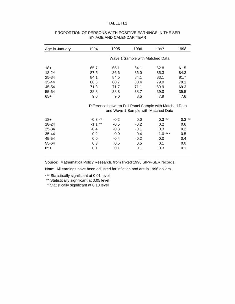
TABLE H.1

PROPORTION OF PERSONS WITH POSITIVE EARNINGS IN THE SERBY AGE AND CALENDAR YEAR

Age in January 1994 1995 1996 1997 1998

18+ 65.7 65.1 64.1 62.8 61.518-24 87.5 86.6 86.0 85.3 84.325-34 84.1 84.5 84.1 83.1 81.735-44 80.6 80.7 80.4 79.9 79.145-54 71.8 71.7 71.1 69.9 69.355-64 38.8 38.8 38.7 39.0 39.565+ 9.0 9.0 8.5 7.9 7.6

Difference between Full Panel Sample with Matched Dataand Wave 1 Sample with Matched Data

18+ -0.3 ** -0.2 0.0 0.3 ** 0.3 **18-24 -1.1 ** -0.5 -0.2 0.2 0.6 25-34 -0.4 -0.3 -0.1 0.3 0.2 35-44 -0.2 0.0 0.4 1.0 *** 0.5 45-54 0.0 -0.4 -0.2 0.0 0.4 55-64 0.3 0.5 0.5 0.1 0.0 65+ 0.1 0.1 0.1 0.3 0.1

Source: Mathematica Policy Research, from linked 1996 SIPP-SER records.

Note: All earnings have been adjusted for inflation and are in 1996 dollars.

*** Statistically significant at 0.01 level ** Statistically significant at 0.05 level * Statistically significant at 0.10 level

Wave 1 Sample with Matched Data

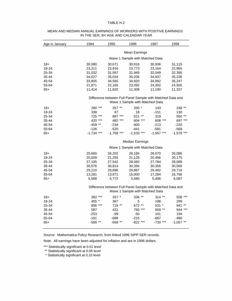
TABLE H.2

MEAN AND MEDIAN ANNUAL EARNINGS OF WORKERS WITH POSITIVE EARNINGS IN THE SER, BY AGE AND CALENDAR YEAR

Age in January 1994 1995 1996 1997 1998

18+ 30,080 30,671 30,916 30,936 31,11518-24 23,211 23,916 23,773 23,164 22,96525-34 31,032 31,597 31,949 32,049 32,39535-44 34,627 35,034 35,036 34,937 35,23645-54 33,805 34,565 34,920 34,992 35,24755-64 21,871 22,165 23,092 24,302 24,50565+ 11,414 11,620 11,308 11,190 11,337

18+ 290 *** 257 ** 200 * 143 248 **18-24 338 87 18 -151 130 25-34 725 *** 687 *** 521 ** 319 550 **35-44 420 *** 482 *** 604 *** 608 *** 697 ***45-54 -459 ** -234 -400 -213 -220 55-64 -126 -520 -441 -581 -568 65+ -1,734 *** -1,769 *** -1,533 *** -1,567 *** -1,578 ***

18+ 25,660 26,202 26,184 26,070 26,08618-24 20,509 21,255 21,129 20,466 20,17525-34 27,105 27,542 28,060 27,784 28,08935-44 30,576 30,814 30,356 30,356 30,56645-54 29,210 29,896 29,867 29,492 29,71955-64 13,281 13,971 15,000 17,284 16,76865+ 5,568 5,772 5,580 5,496 6,087

18+ 382 *** 267 * 336 ** 314 ** 508 ***18-24 455 * 367 5 196 299 25-34 806 *** 719 ** 672 ** 531 * 941 **35-44 587 431 760 *** 659 ** 944 ***45-54 -253 -99 -50 101 194 55-64 -161 -689 -215 -687 -480 65+ -589 ** -658 ** -822 *** -730 *** -1,057 **

Source: Mathematica Policy Research, from linked 1996 SIPP-SER records.

Note: All earnings have been adjusted for inflation and are in 1996 dollars.

*** Statistically significant at 0.01 level ** Statistically significant at 0.05 level * Statistically significant at 0.10 level

Wave 1 Sample with Matched Data

Difference between Full Panel Sample with Matched Data and Wave 1 Sample with Matched Data

Difference between Full Panel Sample with Matched Data and Wave 1 Sample with Matched Data

Wave 1 Sample with Matched Data

Mean Earnings

Median Earnings

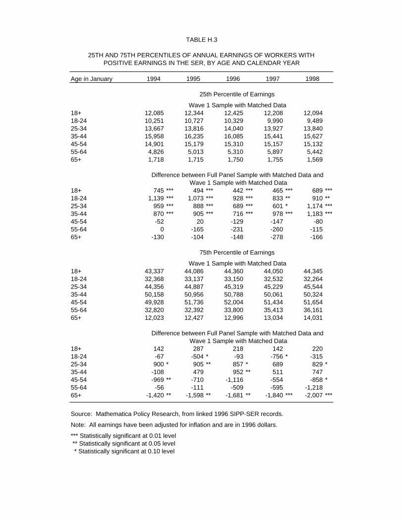
TABLE H.3

25TH AND 75TH PERCENTILES OF ANNUAL EARNINGS OF WORKERS WITHPOSITIVE EARNINGS IN THE SER, BY AGE AND CALENDAR YEAR

Age in January 1994 1995 1996 1997 1998

18+ 12,085 12,344 12,425 12,208 12,09418-24 10,251 10,727 10,329 9,990 9,48925-34 13,667 13,816 14,040 13,927 13,84035-44 15,958 16,235 16,085 15,441 15,62745-54 14,901 15,179 15,310 15,157 15,13255-64 4,826 5,013 5,310 5,897 5,44265+ 1,718 1,715 1,750 1,755 1,569

18+ 745 *** 494 *** 442 *** 465 *** 689 ***18-24 1,139 *** 1,073 *** 928 *** 833 ** 910 **25-34 959 *** 888 *** 689 *** 601 * 1,174 ***35-44 870 *** 905 *** 716 *** 978 *** 1,183 ***45-54 -52 20 -129 -147 -80 55-64 0 -165 -231 -260 -115 65+ -130 -104 -148 -278 -166

18+ 43,337 44,086 44,360 44,050 44,34518-24 32,368 33,137 33,150 32,532 32,26425-34 44,356 44,887 45,319 45,229 45,54435-44 50,158 50,956 50,788 50,061 50,32445-54 49,928 51,736 52,004 51,434 51,65455-64 32,820 32,392 33,800 35,413 36,16165+ 12,023 12,427 12,996 13,034 14,031

18+ 142 287 218 142 220 18-24 -67 -504 * -93 -756 * -315 25-34 900 * 905 ** 857 * 689 829 *35-44 -108 479 952 ** 511 747 45-54 -969 ** -710 -1,116 -554 -858 *55-64 -56 -111 -509 -595 -1,218 65+ -1,420 ** -1,598 ** -1,681 ** -1,840 *** -2,007 ***

Source: Mathematica Policy Research, from linked 1996 SIPP-SER records.

Note: All earnings have been adjusted for inflation and are in 1996 dollars.

*** Statistically significant at 0.01 level ** Statistically significant at 0.05 level * Statistically significant at 0.10 level

Wave 1 Sample with Matched Data

Difference between Full Panel Sample with Matched Data and Wave 1 Sample with Matched Data

Difference between Full Panel Sample with Matched Data and Wave 1 Sample with Matched Data

Wave 1 Sample with Matched Data

25th Percentile of Earnings

75th Percentile of Earnings

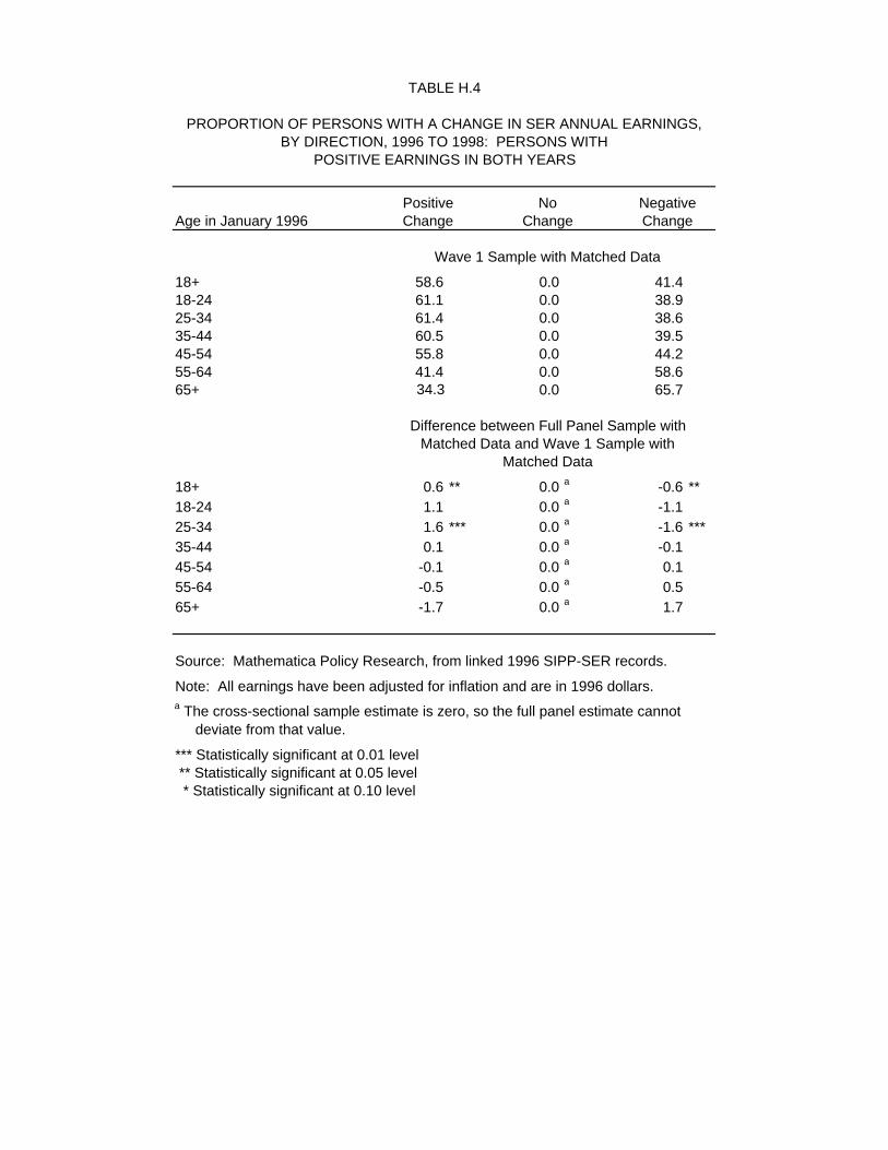
TABLE H.4

PROPORTION OF PERSONS WITH A CHANGE IN SER ANNUAL EARNINGS,BY DIRECTION, 1996 TO 1998: PERSONS WITH

POSITIVE EARNINGS IN BOTH YEARS

Positive No NegativeAge in January 1996 Change Change Change

Wave 1 Sample with Matched Data

18+ 58.6 0.0 41.418-24 61.1 0.0 38.925-34 61.4 0.0 38.635-44 60.5 0.0 39.545-54 55.8 0.0 44.255-64 41.4 0.0 58.665+ 34.3 0.0 65.7

Difference between Full Panel Sample withMatched Data and Wave 1 Sample with

Matched Data

18+ 0.6 ** 0.0 a -0.6 **18-24 1.1 0.0 a -1.1 25-34 1.6 *** 0.0 a -1.6 ***35-44 0.1 0.0 a -0.1 45-54 -0.1 0.0 a 0.1 55-64 -0.5 0.0 a 0.5 65+ -1.7 0.0 a 1.7

Source: Mathematica Policy Research, from linked 1996 SIPP-SER records.

Note: All earnings have been adjusted for inflation and are in 1996 dollars.a The cross-sectional sample estimate is zero, so the full panel estimate cannot deviate from that value.

*** Statistically significant at 0.01 level ** Statistically significant at 0.05 level * Statistically significant at 0.10 level

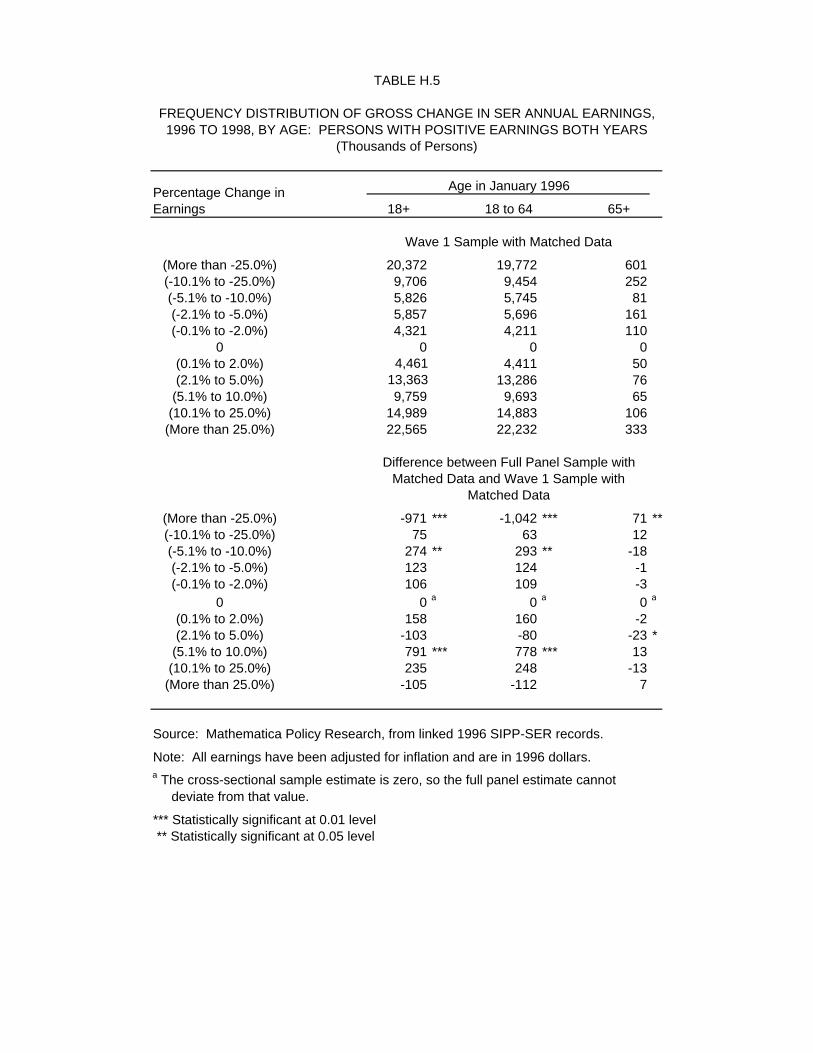
TABLE H.5

FREQUENCY DISTRIBUTION OF GROSS CHANGE IN SER ANNUAL EARNINGS,1996 TO 1998, BY AGE: PERSONS WITH POSITIVE EARNINGS BOTH YEARS

(Thousands of Persons)

Age in January 1996

18+ 18 to 64 65+

Wave 1 Sample with Matched Data

(More than -25.0%) 20,372 19,772 601(-10.1% to -25.0%) 9,706 9,454 252(-5.1% to -10.0%) 5,826 5,745 81(-2.1% to -5.0%) 5,857 5,696 161(-0.1% to -2.0%) 4,321 4,211 110

0 0 0 0(0.1% to 2.0%) 4,461 4,411 50(2.1% to 5.0%) 13,363 13,286 76(5.1% to 10.0%) 9,759 9,693 65(10.1% to 25.0%) 14,989 14,883 106(More than 25.0%) 22,565 22,232 333

Difference between Full Panel Sample withMatched Data and Wave 1 Sample with

Matched Data

(More than -25.0%) -971 *** -1,042 *** 71 **(-10.1% to -25.0%) 75 63 12 (-5.1% to -10.0%) 274 ** 293 ** -18 (-2.1% to -5.0%) 123 124 -1 (-0.1% to -2.0%) 106 109 -3

0 0 a 0 a 0 a

(0.1% to 2.0%) 158 160 -2 (2.1% to 5.0%) -103 -80 -23 *(5.1% to 10.0%) 791 *** 778 *** 13 (10.1% to 25.0%) 235 248 -13 (More than 25.0%) -105 -112 7

Source: Mathematica Policy Research, from linked 1996 SIPP-SER records.

Note: All earnings have been adjusted for inflation and are in 1996 dollars.a The cross-sectional sample estimate is zero, so the full panel estimate cannot deviate from that value.

*** Statistically significant at 0.01 level ** Statistically significant at 0.05 level

Percentage Change in Earnings

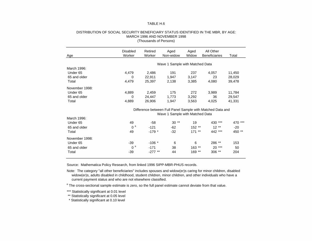
TABLE H.6

DISTRIBUTION OF SOCIAL SECURITY BENEFICIARY STATUS IDENTIFIED IN THE MBR, BY AGE:MARCH 1996 AND NOVEMBER 1998

(Thousands of Persons)

Disabled Retired Aged Aged All OtherAge Worker Worker Non-widow Widow Beneficiaries Total

March 1996: Under 65 4,479 2,486 191 237 4,057 11,450 65 and older 0 22,911 1,947 3,147 23 28,029 Total 4,479 25,397 2,138 3,385 4,080 39,478

November 1998: Under 65 4,889 2,459 175 272 3,989 11,784 65 and older 0 24,447 1,773 3,292 36 29,547 Total 4,889 26,906 1,947 3,563 4,025 41,331

Difference between Full Panel Sample with Matched Data andWave 1 Sample with Matched Data

March 1996: Under 65 49 -58 30 ** 19 430 *** 470 *** 65 and older 0 a -121 -62 152 ** 12 ** -20 Total 49 -179 * -32 171 ** 442 *** 450 **

November 1998: Under 65 -39 -106 * 6 6 286 ** 153 65 and older 0 a -171 38 163 ** 20 *** 50 Total -39 -277 ** 44 169 ** 306 ** 204

Source: Mathematica Policy Research, from linked 1996 SIPP-MBR-PHUS records.

Note: The category "all other beneficiaries" includes spouses and widow(er)s caring for minor children, disabled widow(er)s, adults disabled in childhood, student children, minor children, and other individuals who have a current payment status and who are not elsewhere classified.a The cross-sectional sample estimate is zero, so the full panel estimate cannot deviate from that value.

*** Statistically significant at 0.01 level ** Statistically significant at 0.05 level * Statistically significant at 0.10 level

Wave 1 Sample with Matched Data

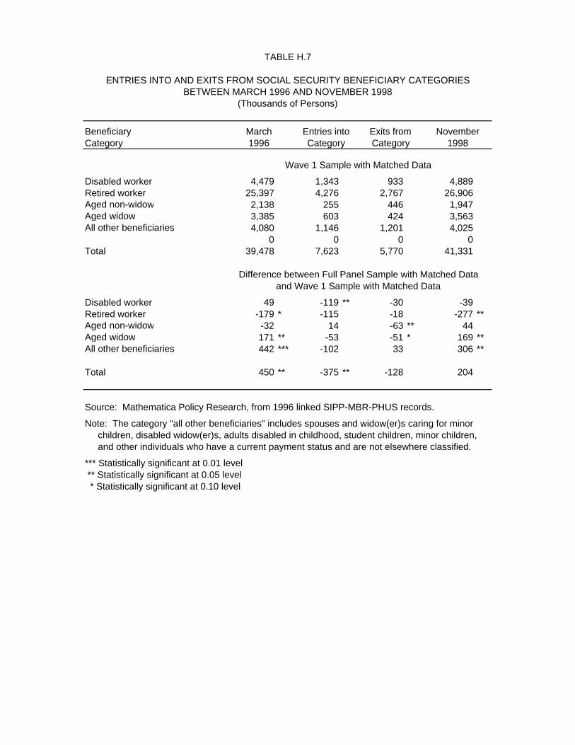
TABLE H.7

ENTRIES INTO AND EXITS FROM SOCIAL SECURITY BENEFICIARY CATEGORIESBETWEEN MARCH 1996 AND NOVEMBER 1998

(Thousands of Persons)

Beneficiary March Entries into Exits from NovemberCategory 1996 Category Category 1998

Wave 1 Sample with Matched Data

Disabled worker 4,479 1,343 933 4,889Retired worker 25,397 4,276 2,767 26,906Aged non-widow 2,138 255 446 1,947Aged widow 3,385 603 424 3,563All other beneficiaries 4,080 1,146 1,201 4,025

0 0 0 0Total 39,478 7,623 5,770 41,331

Difference between Full Panel Sample with Matched Dataand Wave 1 Sample with Matched Data

Disabled worker 49 -119 ** -30 -39 Retired worker -179 * -115 -18 -277 **Aged non-widow -32 14 -63 ** 44 Aged widow 171 ** -53 -51 * 169 **All other beneficiaries 442 *** -102 33 306 **

Total 450 ** -375 ** -128 204

Source: Mathematica Policy Research, from 1996 linked SIPP-MBR-PHUS records.

Note: The category "all other beneficiaries" includes spouses and widow(er)s caring for minor children, disabled widow(er)s, adults disabled in childhood, student children, minor children, and other individuals who have a current payment status and are not elsewhere classified.

*** Statistically significant at 0.01 level ** Statistically significant at 0.05 level * Statistically significant at 0.10 level

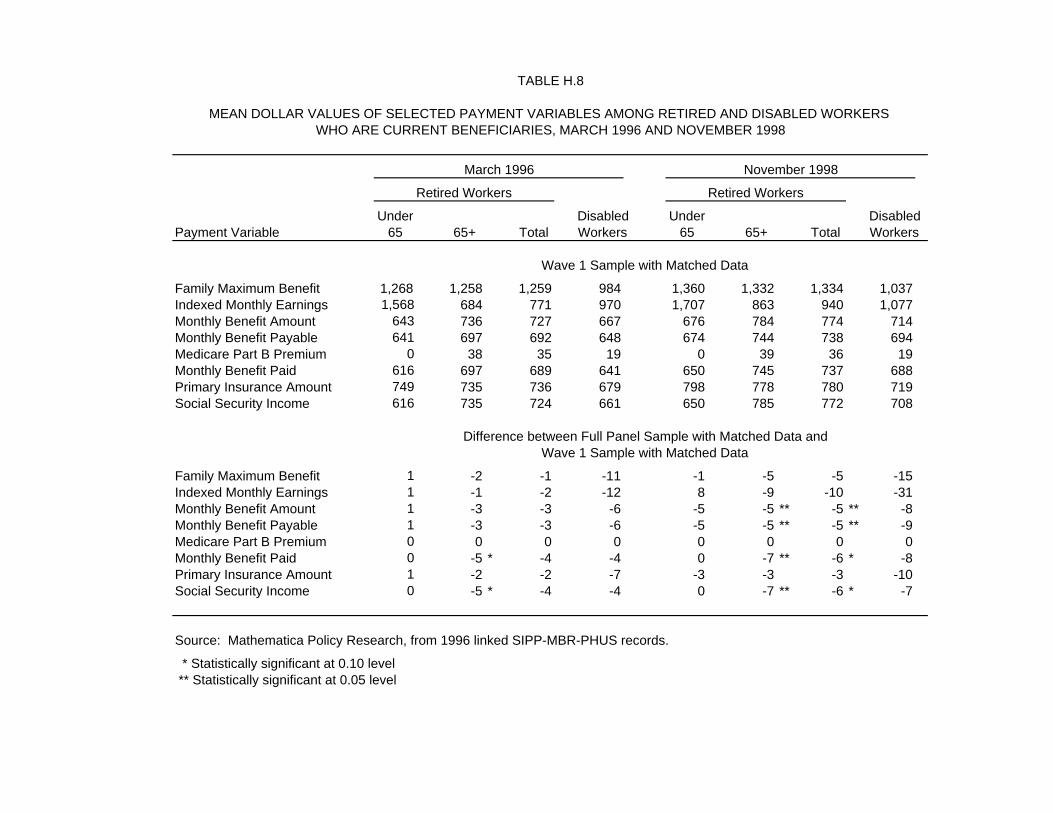
TABLE H.8

MEAN DOLLAR VALUES OF SELECTED PAYMENT VARIABLES AMONG RETIRED AND DISABLED WORKERS WHO ARE CURRENT BENEFICIARIES, MARCH 1996 AND NOVEMBER 1998

March 1996 November 1998

Retired Workers Retired Workers

Under Disabled Under DisabledPayment Variable 65 65+ Total Workers 65 65+ Total Workers

Wave 1 Sample with Matched Data

Family Maximum Benefit 1,268 1,258 1,259 984 1,360 1,332 1,334 1,037Indexed Monthly Earnings 1,568 684 771 970 1,707 863 940 1,077Monthly Benefit Amount 643 736 727 667 676 784 774 714Monthly Benefit Payable 641 697 692 648 674 744 738 694Medicare Part B Premium 0 38 35 19 0 39 36 19Monthly Benefit Paid 616 697 689 641 650 745 737 688Primary Insurance Amount 749 735 736 679 798 778 780 719Social Security Income 616 735 724 661 650 785 772 708

Difference between Full Panel Sample with Matched Data andWave 1 Sample with Matched Data

Family Maximum Benefit 1 -2 -1 -11 -1 -5 -5 -15 Indexed Monthly Earnings 1 -1 -2 -12 8 -9 -10 -31 Monthly Benefit Amount 1 -3 -3 -6 -5 -5 ** -5 ** -8 Monthly Benefit Payable 1 -3 -3 -6 -5 -5 ** -5 ** -9 Medicare Part B Premium 0 0 0 0 0 0 0 0 Monthly Benefit Paid 0 -5 * -4 -4 0 -7 ** -6 * -8 Primary Insurance Amount 1 -2 -2 -7 -3 -3 -3 -10 Social Security Income 0 -5 * -4 -4 0 -7 ** -6 * -7

Source: Mathematica Policy Research, from 1996 linked SIPP-MBR-PHUS records.

* Statistically significant at 0.10 level ** Statistically significant at 0.05 level

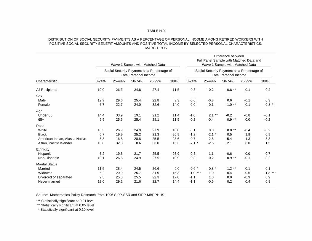
DISTRIBUTION OF SOCIAL SECURITY PAYMENTS AS A PERCENTAGE OF PERSONAL INCOME AMONG RETIRED WORKERS WITHPOSITIVE SOCIAL SECURITY BENEFIT AMOUNTS AND POSITIVE TOTAL INCOME BY SELECTED PERSONAL CHARACTERISTICS:

MARCH 1996

Difference betweenFull Panel Sample with Matched Data and

Wave 1 Sample with Matched Data Wave 1 Sample with Matched Data

Social Security Payment as a Percentage of Social Security Payment as a Percentage ofTotal Personal Income Total Personal Income

Characteristic 0-24% 25-49% 50-74% 75-99% 100% 0-24% 25-49% 50-74% 75-99% 100%

All Recipients 10.0 26.3 24.8 27.4 11.5 -0.3 -0.2 0.8 ** -0.1 -0.2

Sex Male 12.9 29.6 25.4 22.8 9.3 -0.6 -0.3 0.6 -0.1 0.3 Female 6.7 22.7 24.0 32.6 14.0 0.0 -0.1 1.0 ** -0.1 -0.8 *

Age Under 65 14.4 33.9 19.1 21.2 11.4 -1.0 2.1 ** -0.2 -0.8 -0.1 65+ 9.5 25.5 25.4 28.1 11.5 -0.2 -0.4 0.9 ** 0.0 -0.2

Race White 10.3 26.9 24.9 27.9 10.0 -0.1 0.0 0.8 ** -0.4 -0.2 Black 6.7 19.9 25.2 21.3 26.9 -1.2 -2.1 * 0.5 1.8 0.9 American Indian, Alaska Native 5.3 16.8 28.8 25.5 23.6 -0.7 2.5 5.4 -1.3 -5.8 Asian, Pacific Islander 10.8 32.3 8.6 33.0 15.3 -7.1 * -2.5 2.1 6.0 1.5

Ethnicity Hispanic 6.2 19.8 21.7 25.5 26.9 0.3 1.1 -0.6 0.0 -0.7 Non-Hispanic 10.1 26.6 24.9 27.5 10.9 -0.3 -0.2 0.9 ** -0.1 -0.2

Marital Status Married 11.5 28.4 24.5 26.6 9.0 -0.6 * -0.8 * 1.2 ** 0.1 0.1 Widowed 6.2 20.9 25.7 31.9 15.3 1.0 *** 1.0 0.4 -0.5 -1.8 *** Divorced or separated 9.3 25.8 25.5 22.3 17.0 -1.1 1.0 0.0 -0.9 0.9 Never married 12.0 29.2 21.6 22.7 14.4 -1.1 -0.5 0.2 0.4 0.9

Source: Mathematica Policy Research, from 1996 SIPP-SSR and SIPP-MBRPHUS.

*** Statistically significant at 0.01 level ** Statistically significant at 0.05 level * Statistically significant at 0.10 level

TABLE H.9

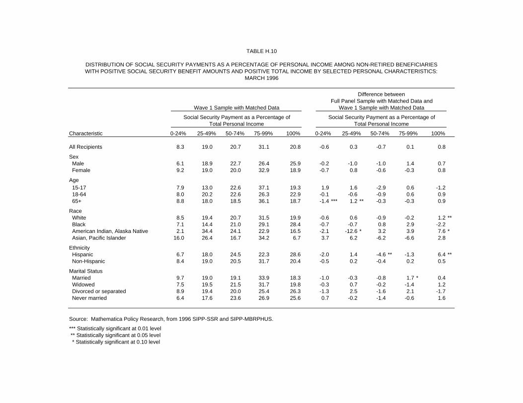
DISTRIBUTION OF SOCIAL SECURITY PAYMENTS AS A PERCENTAGE OF PERSONAL INCOME AMONG NON-RETIRED BENEFICIARIESWITH POSITIVE SOCIAL SECURITY BENEFIT AMOUNTS AND POSITIVE TOTAL INCOME BY SELECTED PERSONAL CHARACTERISTICS:

MARCH 1996

Difference betweenFull Panel Sample with Matched Data and

Wave 1 Sample with Matched Data Wave 1 Sample with Matched Data

Social Security Payment as a Percentage of Social Security Payment as a Percentage ofTotal Personal Income Total Personal Income

Characteristic 0-24% 25-49% 50-74% 75-99% 100% 0-24% 25-49% 50-74% 75-99% 100%

All Recipients 8.3 19.0 20.7 31.1 20.8 -0.6 0.3 -0.7 0.1 0.8

Sex Male 6.1 18.9 22.7 26.4 25.9 -0.2 -1.0 -1.0 1.4 0.7 Female 9.2 19.0 20.0 32.9 18.9 -0.7 0.8 -0.6 -0.3 0.8

Age 15-17 7.9 13.0 22.6 37.1 19.3 1.9 1.6 -2.9 0.6 -1.2 18-64 8.0 20.2 22.6 26.3 22.9 -0.1 -0.6 -0.9 0.6 0.9 65+ 8.8 18.0 18.5 36.1 18.7 -1.4 *** 1.2 ** -0.3 -0.3 0.9

Race White 8.5 19.4 20.7 31.5 19.9 -0.6 0.6 -0.9 -0.2 1.2 ** Black 7.1 14.4 21.0 29.1 28.4 -0.7 -0.7 0.8 2.9 -2.2 American Indian, Alaska Native 2.1 34.4 24.1 22.9 16.5 -2.1 -12.6 * 3.2 3.9 7.6 * Asian, Pacific Islander 16.0 26.4 16.7 34.2 6.7 3.7 6.2 -6.2 -6.6 2.8

Ethnicity Hispanic 6.7 18.0 24.5 22.3 28.6 -2.0 1.4 -4.6 ** -1.3 6.4 ** Non-Hispanic 8.4 19.0 20.5 31.7 20.4 -0.5 0.2 -0.4 0.2 0.5

Marital Status Married 9.7 19.0 19.1 33.9 18.3 -1.0 -0.3 -0.8 1.7 * 0.4 Widowed 7.5 19.5 21.5 31.7 19.8 -0.3 0.7 -0.2 -1.4 1.2 Divorced or separated 8.9 19.4 20.0 25.4 26.3 -1.3 2.5 -1.6 2.1 -1.7 Never married 6.4 17.6 23.6 26.9 25.6 0.7 -0.2 -1.4 -0.6 1.6

Source: Mathematica Policy Research, from 1996 SIPP-SSR and SIPP-MBRPHUS.

*** Statistically significant at 0.01 level ** Statistically significant at 0.05 level * Statistically significant at 0.10 level

TABLE H.10

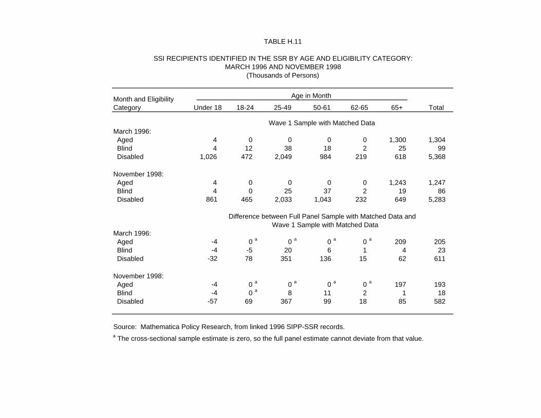
TABLE H.11

SSI RECIPIENTS IDENTIFIED IN THE SSR BY AGE AND ELIGIBILITY CATEGORY:MARCH 1996 AND NOVEMBER 1998

(Thousands of Persons)

Age in Month

Under 18 18-24 25-49 50-61 62-65 65+ Total

Wave 1 Sample with Matched DataMarch 1996: Aged 4 0 0 0 0 1,300 1,304 Blind 4 12 38 18 2 25 99 Disabled 1,026 472 2,049 984 219 618 5,368 November 1998: Aged 4 0 0 0 0 1,243 1,247 Blind 4 0 25 37 2 19 86 Disabled 861 465 2,033 1,043 232 649 5,283

Difference between Full Panel Sample with Matched Data and

March 1996: Aged -4 0 a 0 a 0 a 0 a 209 205 Blind -4 -5 20 6 1 4 23 Disabled -32 78 351 136 15 62 611 November 1998: Aged -4 0 a 0 a 0 a 0 a 197 193 Blind -4 0 a 8 11 2 1 18 Disabled -57 69 367 99 18 85 582

Source: Mathematica Policy Research, from linked 1996 SIPP-SSR records.a The cross-sectional sample estimate is zero, so the full panel estimate cannot deviate from that value.

Month and Eligibility Category

Wave 1 Sample with Matched Data

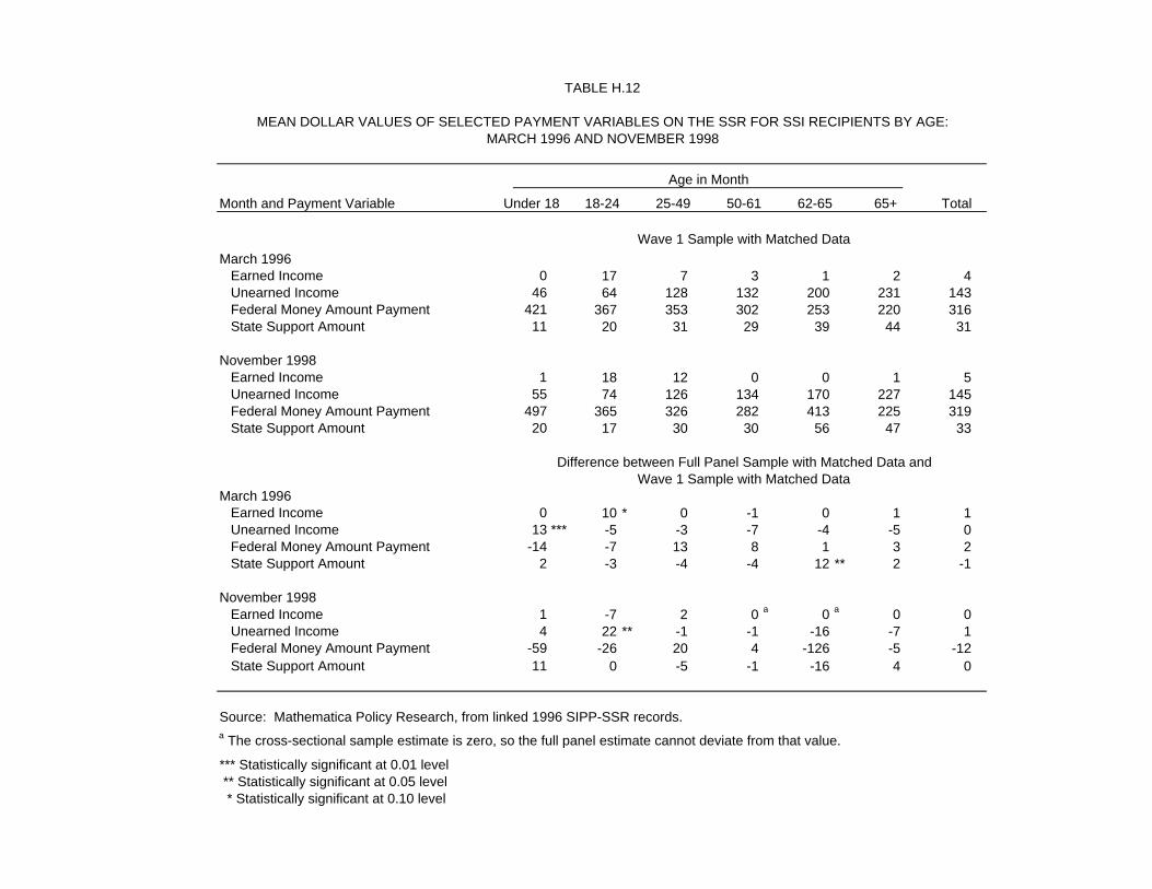
TABLE H.12

MEAN DOLLAR VALUES OF SELECTED PAYMENT VARIABLES ON THE SSR FOR SSI RECIPIENTS BY AGE:MARCH 1996 AND NOVEMBER 1998

Age in Month

Month and Payment Variable Under 18 18-24 25-49 50-61 62-65 65+ Total

Wave 1 Sample with Matched Data

March 1996 Earned Income 0 17 7 3 1 2 4 Unearned Income 46 64 128 132 200 231 143 Federal Money Amount Payment 421 367 353 302 253 220 316 State Support Amount 11 20 31 29 39 44 31

November 1998 Earned Income 1 18 12 0 0 1 5 Unearned Income 55 74 126 134 170 227 145 Federal Money Amount Payment 497 365 326 282 413 225 319 State Support Amount 20 17 30 30 56 47 33

Difference between Full Panel Sample with Matched Data andWave 1 Sample with Matched Data

March 1996 Earned Income 0 10 * 0 -1 0 1 1 Unearned Income 13 *** -5 -3 -7 -4 -5 0 Federal Money Amount Payment -14 -7 13 8 1 3 2 State Support Amount 2 -3 -4 -4 12 ** 2 -1

November 1998 Earned Income 1 -7 2 0 a 0 a 0 0 Unearned Income 4 22 ** -1 -1 -16 -7 1 Federal Money Amount Payment -59 -26 20 4 -126 -5 -12 State Support Amount 11 0 -5 -1 -16 4 0

Source: Mathematica Policy Research, from linked 1996 SIPP-SSR records.a The cross-sectional sample estimate is zero, so the full panel estimate cannot deviate from that value.

*** Statistically significant at 0.01 level ** Statistically significant at 0.05 level * Statistically significant at 0.10 level

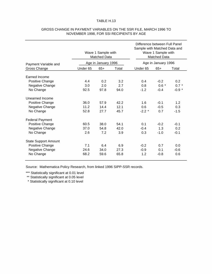
TABLE H.13

GROSS CHANGE IN PAYMENT VARIABLES ON THE SSR FILE, MARCH 1996 TONOVEMBER 1998, FOR SSI RECIPIENTS BY AGE

Difference between Full PanelSample with Matched Data and

Wave 1 Sample with Wave 1 Sample withMatched Data Matched Data

Age in January 1996 Age in January 1996

Under 65 65+ Total Under 65 65+ Total

Earned Income Positive Change 4.4 0.2 3.2 0.4 -0.2 0.2 Negative Change 3.0 2.0 2.7 0.8 0.6 * 0.7 * No Change 92.5 97.8 94.0 -1.2 -0.4 -0.9 *

Unearned Income Positive Change 36.0 57.9 42.2 1.6 -0.1 1.2 Negative Change 11.2 14.4 12.1 0.6 -0.5 0.3 No Change 52.8 27.7 45.7 -2.2 * 0.7 -1.5

Federal Payment Positive Change 60.5 38.0 54.1 0.1 -0.2 -0.1 Negative Change 37.0 54.8 42.0 -0.4 1.3 0.2 No Change 2.6 7.2 3.9 0.3 -1.0 -0.1

State Support Amount Positive Change 7.1 6.4 6.9 -0.2 0.7 0.0 Negative Change 24.6 34.0 27.3 -0.9 0.1 -0.6 No Change 68.2 59.6 65.8 1.2 -0.8 0.6

Source: Mathematica Policy Research, from linked 1996 SIPP-SSR records.

*** Statistically significant at 0.01 level ** Statistically significant at 0.05 level * Statistically significant at 0.10 level

Payment Variable and Gross Change

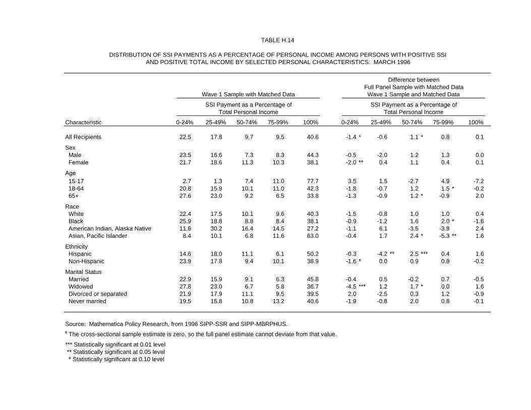
DISTRIBUTION OF SSI PAYMENTS AS A PERCENTAGE OF PERSONAL INCOME AMONG PERSONS WITH POSITIVE SSIAND POSITIVE TOTAL INCOME BY SELECTED PERSONAL CHARACTERISTICS: MARCH 1996

Difference betweenFull Panel Sample with Matched Data

Wave 1 Sample with Matched Data Wave 1 Sample and Matched Data

SSI Payment as a Percentage of SSI Payment as a Percentage ofTotal Personal Income Total Personal Income

Characteristic 0-24% 25-49% 50-74% 75-99% 100% 0-24% 25-49% 50-74% 75-99% 100%

All Recipients 22.5 17.8 9.7 9.5 40.6 -1.4 * -0.6 1.1 * 0.8 0.1

Sex Male 23.5 16.6 7.3 8.3 44.3 -0.5 -2.0 1.2 1.3 0.0 Female 21.7 18.6 11.3 10.3 38.1 -2.0 ** 0.4 1.1 0.4 0.1

Age 15-17 2.7 1.3 7.4 11.0 77.7 3.5 1.5 -2.7 4.9 -7.2 18-64 20.8 15.9 10.1 11.0 42.3 -1.8 -0.7 1.2 1.5 * -0.2 65+ 27.6 23.0 9.2 6.5 33.8 -1.3 -0.9 1.2 * -0.9 2.0

Race White 22.4 17.5 10.1 9.6 40.3 -1.5 -0.8 1.0 1.0 0.4 Black 25.9 18.8 8.8 8.4 38.1 -0.9 -1.2 1.6 2.0 * -1.6 American Indian, Alaska Native 11.6 30.2 16.4 14.5 27.2 -1.1 6.1 -3.5 -3.9 2.4 Asian, Pacific Islander 8.4 10.1 6.8 11.6 63.0 -0.4 1.7 2.4 * -5.3 ** 1.6

Ethnicity Hispanic 14.6 18.0 11.1 6.1 50.2 -0.3 -4.2 ** 2.5 *** 0.4 1.6 Non-Hispanic 23.9 17.8 9.4 10.1 38.9 -1.6 * 0.0 0.9 0.8 -0.2

Marital Status Married 22.9 15.9 9.1 6.3 45.8 -0.4 0.5 -0.2 0.7 -0.5 Widowed 27.8 23.0 6.7 5.8 36.7 -4.5 *** 1.2 1.7 * 0.0 1.6 Divorced or separated 21.9 17.9 11.1 9.5 39.5 2.0 -2.5 0.3 1.2 -0.9 Never married 19.5 15.8 10.8 13.2 40.6 -1.9 -0.8 2.0 0.8 -0.1

Source: Mathematica Policy Research, from 1996 SIPP-SSR and SIPP-MBRPHUS.a The cross-sectional sample estimate is zero, so the full panel estimate cannot deviate from that value.

*** Statistically significant at 0.01 level ** Statistically significant at 0.05 level * Statistically significant at 0.10 level

TABLE H.14

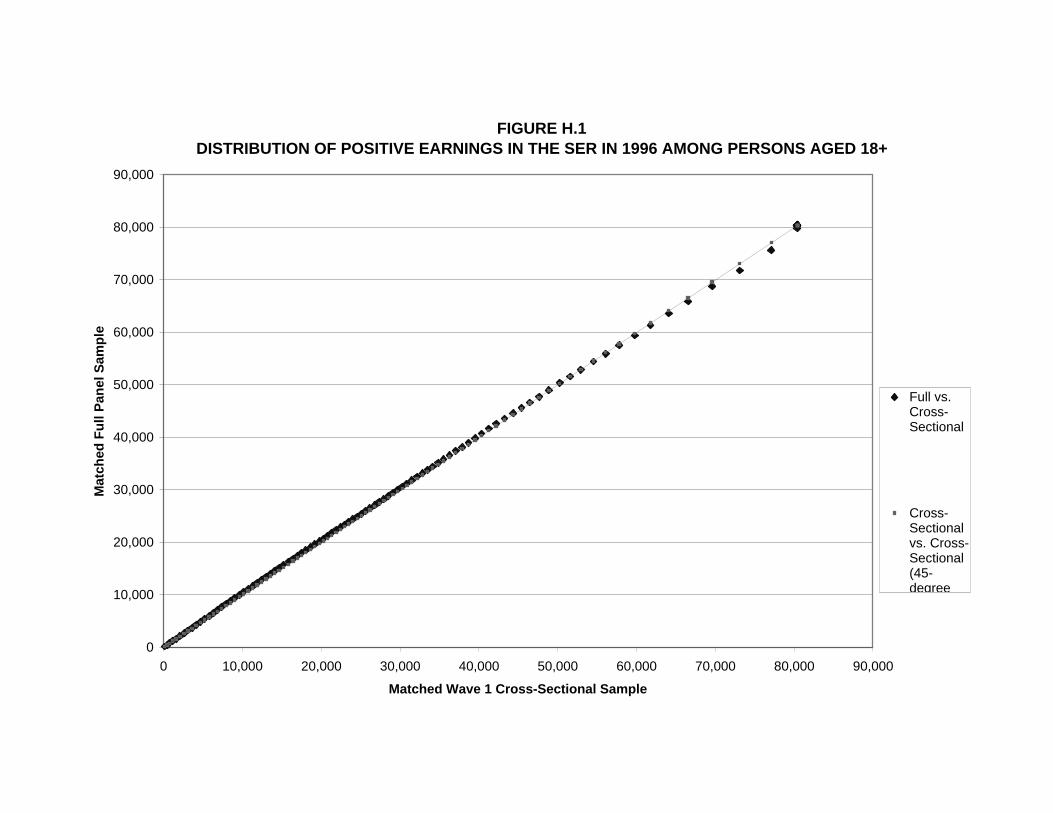
FIGURE H.1DISTRIBUTION OF POSITIVE EARNINGS IN THE SER IN 1996 AMONG PERSONS AGED 18+

0

10,000

20,000

30,000

40,000

50,000

60,000

70,000

80,000

90,000

0 10,000 20,000 30,000 40,000 50,000 60,000 70,000 80,000 90,000

Matched Wave 1 Cross-Sectional Sample

Mat

ched

Fu

ll P

anel

Sam

ple

Full vs.Cross-Sectional

Cross-Sectionalvs. Cross-Sectional(45-degree

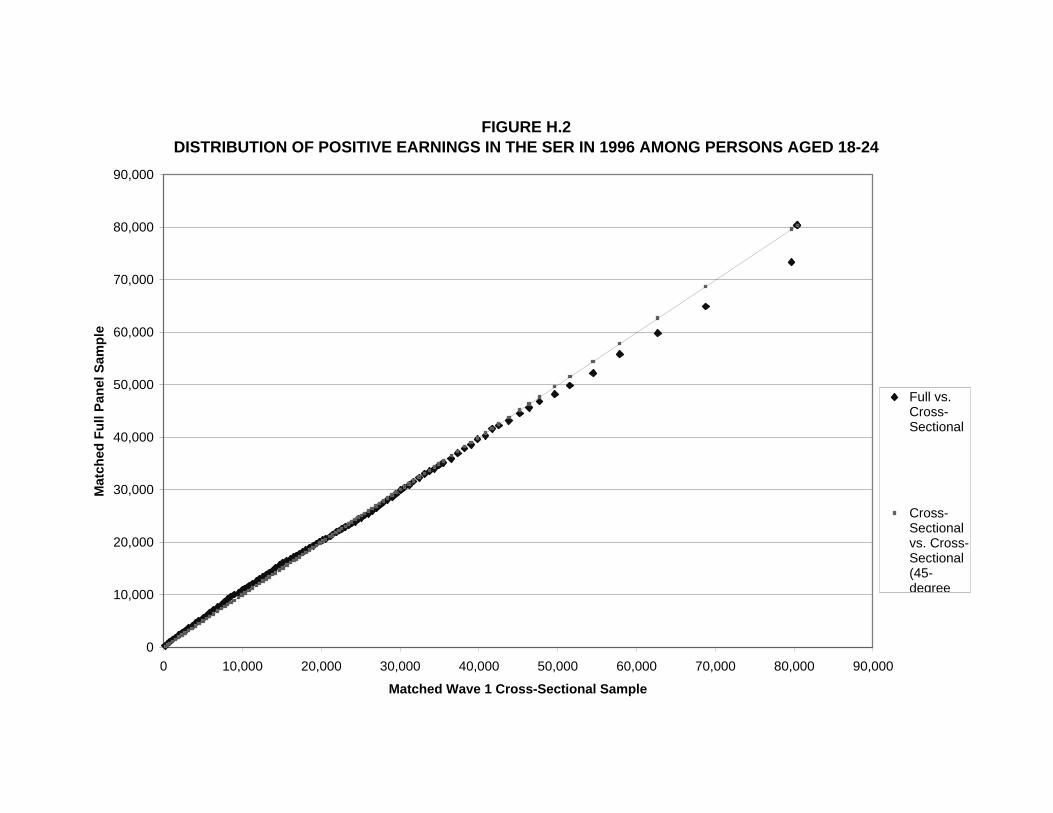
FIGURE H.2DISTRIBUTION OF POSITIVE EARNINGS IN THE SER IN 1996 AMONG PERSONS AGED 18-24

0

10,000

20,000

30,000

40,000

50,000

60,000

70,000

80,000

90,000

0 10,000 20,000 30,000 40,000 50,000 60,000 70,000 80,000 90,000

Matched Wave 1 Cross-Sectional Sample

Mat

ched

Fu

ll P

anel

Sam

ple

Full vs.Cross-Sectional

Cross-Sectionalvs. Cross-Sectional(45-degree

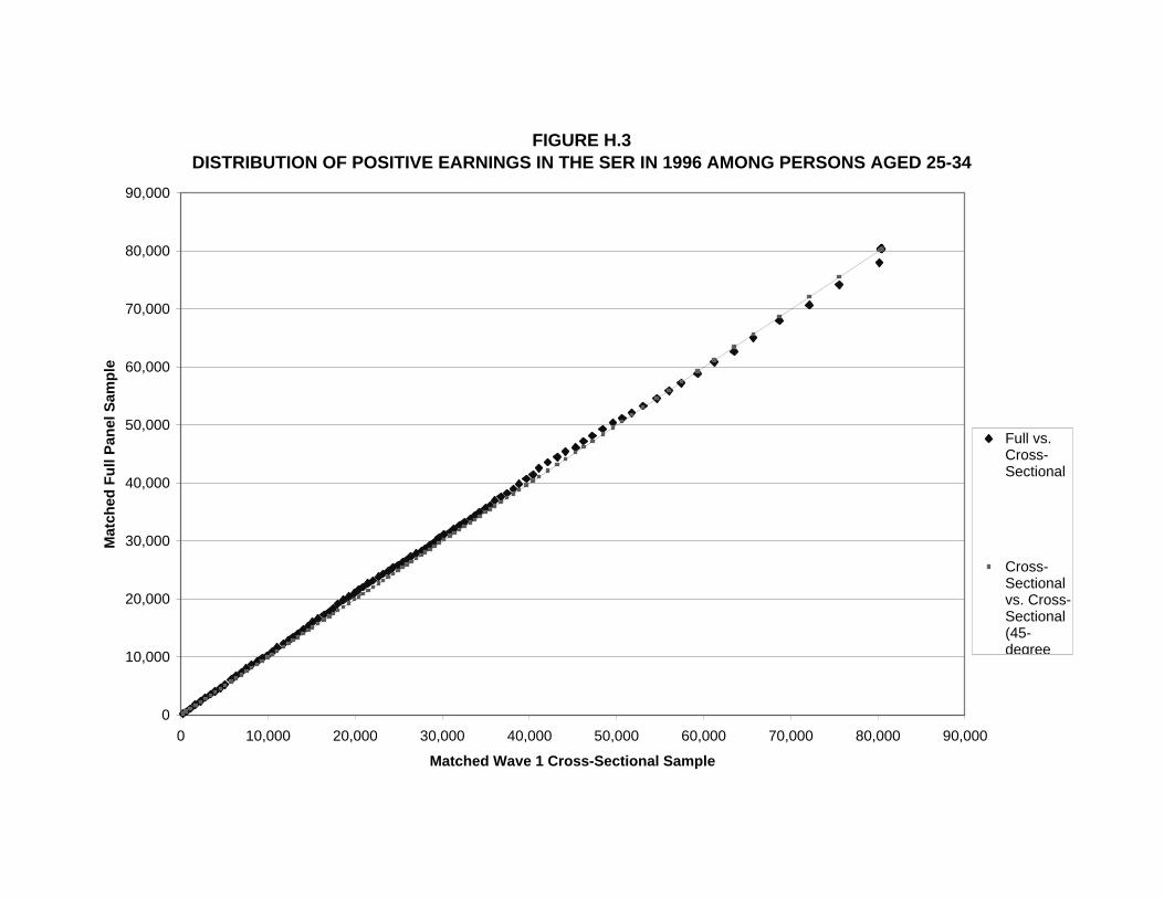
FIGURE H.3DISTRIBUTION OF POSITIVE EARNINGS IN THE SER IN 1996 AMONG PERSONS AGED 25-34

0

10,000

20,000

30,000

40,000

50,000

60,000

70,000

80,000

90,000

0 10,000 20,000 30,000 40,000 50,000 60,000 70,000 80,000 90,000

Matched Wave 1 Cross-Sectional Sample

Mat

ched

Fu

ll P

anel

Sam

ple

Full vs.Cross-Sectional

Cross-Sectionalvs. Cross-Sectional(45-degree

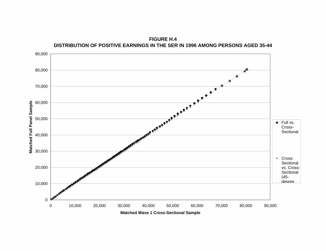
FIGURE H.4DISTRIBUTION OF POSITIVE EARNINGS IN THE SER IN 1996 AMONG PERSONS AGED 35-44

0

10,000

20,000

30,000

40,000

50,000

60,000

70,000

80,000

90,000

0 10,000 20,000 30,000 40,000 50,000 60,000 70,000 80,000 90,000

Matched Wave 1 Cross-Sectional Sample

Mat

ched

Fu

ll P

anel

Sam

ple

Full vs.Cross-Sectional

Cross-Sectionalvs. Cross-Sectional(45-degree

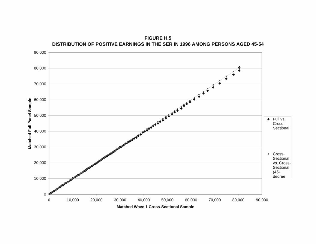
FIGURE H.5DISTRIBUTION OF POSITIVE EARNINGS IN THE SER IN 1996 AMONG PERSONS AGED 45-54

0

10,000

20,000

30,000

40,000

50,000

60,000

70,000

80,000

90,000

0 10,000 20,000 30,000 40,000 50,000 60,000 70,000 80,000 90,000

Matched Wave 1 Cross-Sectional Sample

Mat

ched

Fu

ll P

anel

Sam

ple

Full vs.Cross-Sectional

Cross-Sectionalvs. Cross-Sectional(45-degree

FIGURE H.6DISTRIBUTION OF POSITIVE EARNINGS IN THE SER IN 1996 AMONG PERSONS AGED 55-64

0

10,000

20,000

30,000

40,000

50,000

60,000

70,000

80,000

90,000

0 10,000 20,000 30,000 40,000 50,000 60,000 70,000 80,000 90,000

Matched Wave 1 Cross-Sectional Sample

Mat

ched

Fu

ll P

anel

Sam

ple

Full vs.Cross-Sectional

Cross-Sectionalvs. Cross-Sectional(45-degree

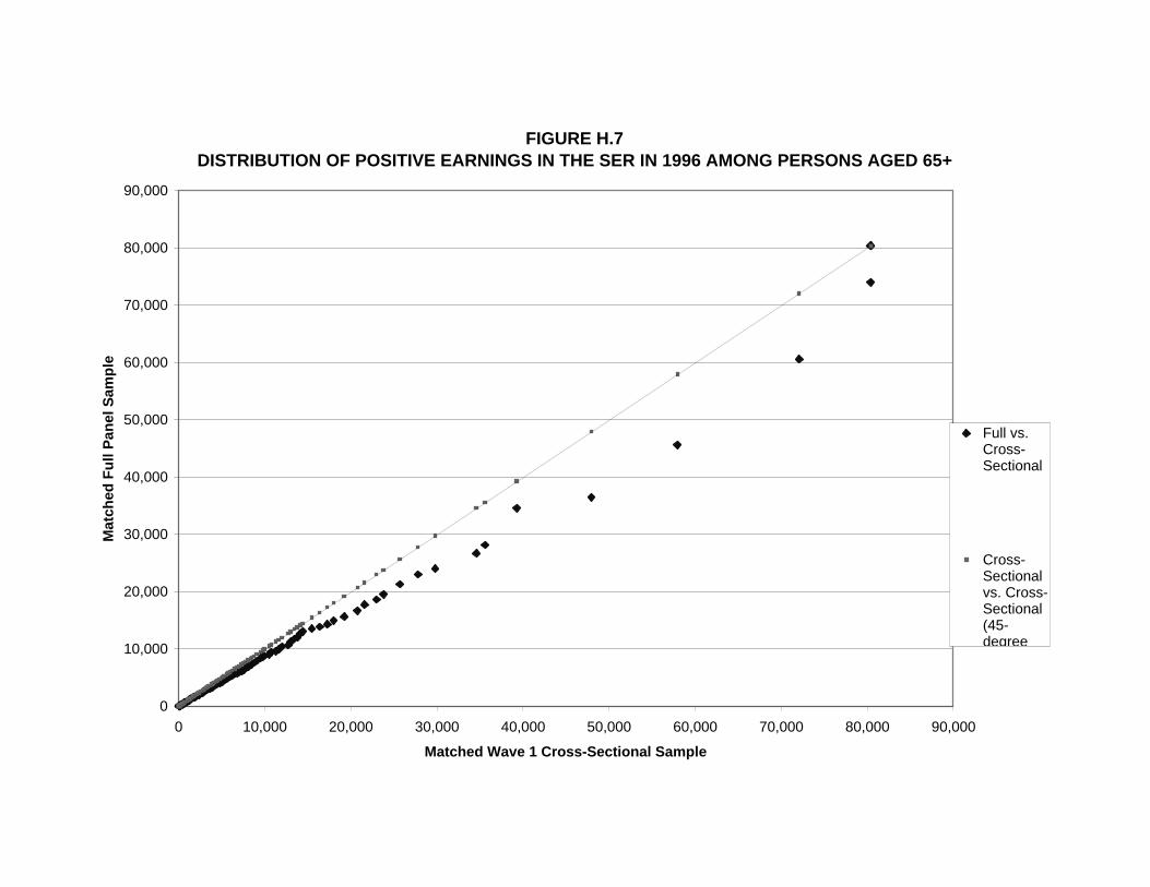
FIGURE H.7DISTRIBUTION OF POSITIVE EARNINGS IN THE SER IN 1996 AMONG PERSONS AGED 65+

0

10,000

20,000

30,000

40,000

50,000

60,000

70,000

80,000

90,000

0 10,000 20,000 30,000 40,000 50,000 60,000 70,000 80,000 90,000

Matched Wave 1 Cross-Sectional Sample

Mat

ched

Fu

ll P

anel

Sam

ple

Full vs.Cross-Sectional

Cross-Sectionalvs. Cross-Sectional(45-degree