THE ECONOMICS

OF AN INDUSTRY

(PERFECTLY

COMPETITIVE)

ENTRY OF FIRMS

EXIT OF FIRMS

LR INDUSTRY

EQUILIBRIUM

ENTRY: When existing firms make SR profit ⇒ P > Min ATCLR (above normal profit)

- LR: new firms entering increases market/industry supply (SHIFT MKT S RIGHT)

o Firms stop entering when market P falls to equal Min ATC

EXIT: When existing firms make SR loss ⇒ P < Min ATCLR (less than normal profit)

- LR: new firms exiting decreases market/industry supply (SHIFT MKT S LEFT)

o Firms stop exiting when market P rises to equal Min ATC

A model of firms in an industry in which free entry and exit leads to an equilibrium where PRICE = Min ATC = LR MC (0 economic profit);

equilibrium occurs when there is no incentive for firms to enter and exit

ASSUMPTIONS: firms maximise profit, individual firms are price takers, and demand for a firm is perfectly elastic, Sindustry is horizontal summation of Sfirms

DESIRABLE FEATURES: ATCLR minimised (so price paid is minimised), capital allocated efficiently (where profit is best)

SAMPLE

IMPACT OF INCREASE

IN MARKET DEMAND

IMPACT OF DECREASE

IN MARKET DEMAND

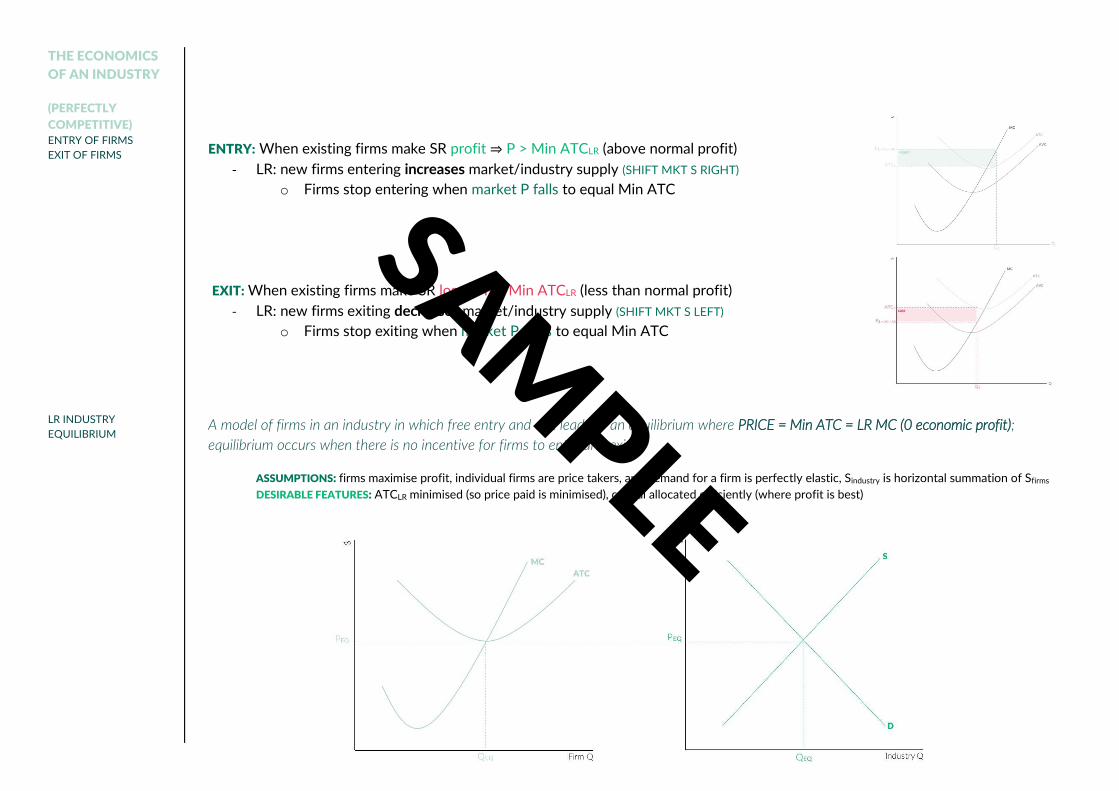
1. D ⇑ due to a non-price factor (shifts to D2), ⇑ P (= ATCMIN)

2. P > ATCMIN so firms make positive profits in SR

SHORT RUN RESULT:

- Increased market price and quantity D/S

3. Firms enter industry in LR, ⇑ market supply (S ⇢ S2) in LR

4. Entry stops (supply increase stops) when P = ATCMIN

LONG RUN RESULT:

- More firms in market (higher market supply QLR)

- Price returns to equilibrium (normal profit)

1. D ⇓ due to a non-price factor (shifts to D2), ⇓ P (= ATCMIN)

2. P < ATCMIN so firms make negative profits in SR

SHORT RUN RESULT:

- Decreased market price and quantity D/S

3. Firms exit industry in LR, ⇓ market supply (S ⇢ S2) in LR

4. Exit stops (supply decrease stops) when P = ATCMIN

LONG RUN RESULT:

- Fewer firms in market (lower market supply QLR)

- Price returns to equilibrium (normal profit)

SR

LR

LR

SR

SAMPLE

IMPACT OF CHANGES

IN COSTS

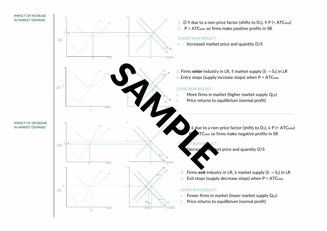
NOTE

In reality, an industry grows or shrinks due to a combination of a change in the number of firms and the expansion/contraction of

existing firms. Expansion can be the result of:

- Firms reducing costs while increasing output (reaching minimum efficient scale, see diseconomies of scale)

- Improved technology or lowered costs of inputs which alter the cost curve and shift minimum efficient scale to higher output

SHORT RUN

1. ↓ Cost in firm – shift down MC and ATC

2. Results in positive profits at P

3. As more firms (entire industry) ↓ Cost,

market S ↑ and market price ↓ to P2

4. There are still positive profits at P2 so firms

enter market over the long run

SHORT RUN RESULT:

- High level of profit and increased output

levels

LONG RUN

5. With entry of firms, market S ↑ in over time

6. Price ↓ further till min ATC is reached

(normal profit) and there is no longer incentive

for firms to enter – P3

LONG RUN RESULT:

- Profit is eroded by competition by entering

firms and normal profit is made again

SAMPLE

LONG RUN INDUSTRY

SUPPLY CURVE

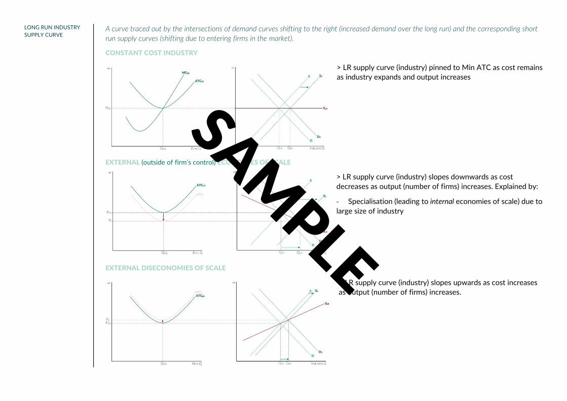
A curve traced out by the intersections of demand curves shifting to the right (increased demand over the long run) and the corresponding short

run supply curves (shifting due to entering firms in the market).

CONSTANT COST INDUSTRY

> LR supply curve (industry) pinned to Min ATC as cost remains

as industry expands and output increases

EXTERNAL (outside of firm’s control) ECONOMIES OF SCALE

> LR supply curve (industry) slopes downwards as cost

decreases as output (number of firms) increases. Explained by:

- Specialisation (leading to internal economies of scale) due to

large size of industry

EXTERNAL DISECONOMIES OF SCALE

> LR supply curve (industry) slopes upwards as cost increases

as output (number of firms) increases.

SAMPLE

MONOPOLIES

REASONS FOR A

MONOPOLY

(BARRIERS TO ENTRY)

1. NATURAL MONOPOLIES occurring due to economies of scale (ATC falls as output rises)

- The market is most cheaply served by a single firm

- Minimum efficient scale is greater than the size of the market (number of consumers) as initial fixed cost is very large while

later running costs are low e.g. electricity and water companies

2. Exclusive access to vital inputs or technology (“industry secrets”) required for production e.g. rare earth minerals

3. Patents and copyright

- Stimulates innovation by rewarding the inventor

4. Government licences e.g. casinos and airports

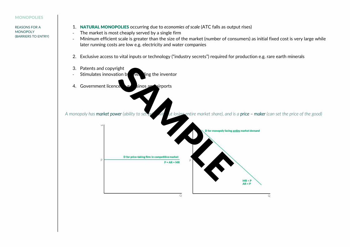
A monopoly has market power (ability to set price without losing entire market share), and is a price – maker (can set the price of the good)

SAMPLE

REVENUE

PROFIT

Marginal revenue falls as output increases till MR is negative

- To sell more, the monopolist must lower the price; at higher quantities the price is lowered greater amounts thus revenue rises

by smaller amounts

- MR curve is linear, it lies below the demand curve and it’s slope is twice as steep as the D

Marginal revenue < Price (except at the first unit of input)

- MR = dRev

dQ=

d P(Q).Q

dQ= P + Q

dP

dQ (by the product rule) ∴ MR = P + Q

dP

dQ < P as

dP

dQ is the slope of the D curve (negative)

Monopolists always operate on elastic portion of Demand curve

- Given MR = P + QdP

dQ = 𝑃 [1 +

𝑄

𝑃∙

𝑑𝑃

𝑑𝑄]

- and 𝜀𝐷= −𝑃

𝑄∙

𝑑𝑄

𝑑𝑃 ∴ MR = 𝑃 [1 −

1

𝜀𝐷]

o if MR > 0, 1

𝜀𝐷< 1therefore, price elasticity of demand is > 1 (elastic D)

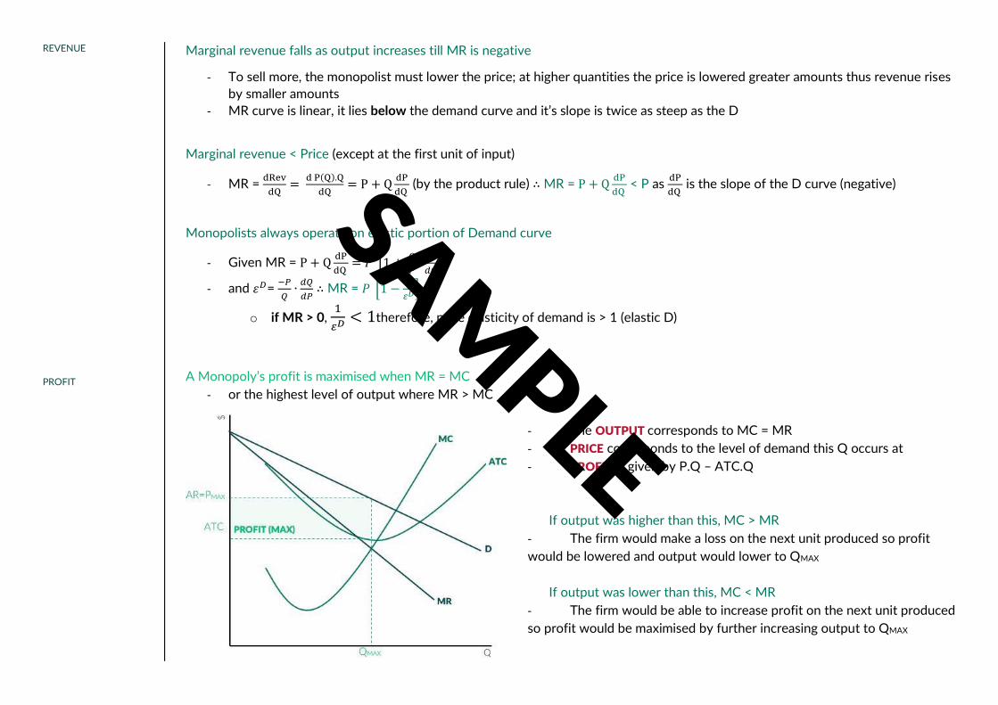
A Monopoly’s profit is maximised when MR = MC

- or the highest level of output where MR > MC

- The OUTPUT corresponds to MC = MR

- PRICE corresponds to the level of demand this Q occurs at

- PROFIT is given by P.Q – ATC.Q

If output was higher than this, MC > MR

- The firm would make a loss on the next unit produced so profit

would be lowered and output would lower to QMAX

If output was lower than this, MC < MR

- The firm would be able to increase profit on the next unit produced

so profit would be maximised by further increasing output to QMAX

SAMPLE

INEFFICIENCY IN A

MONOPOLY

PRICE

DISCRIMINATION

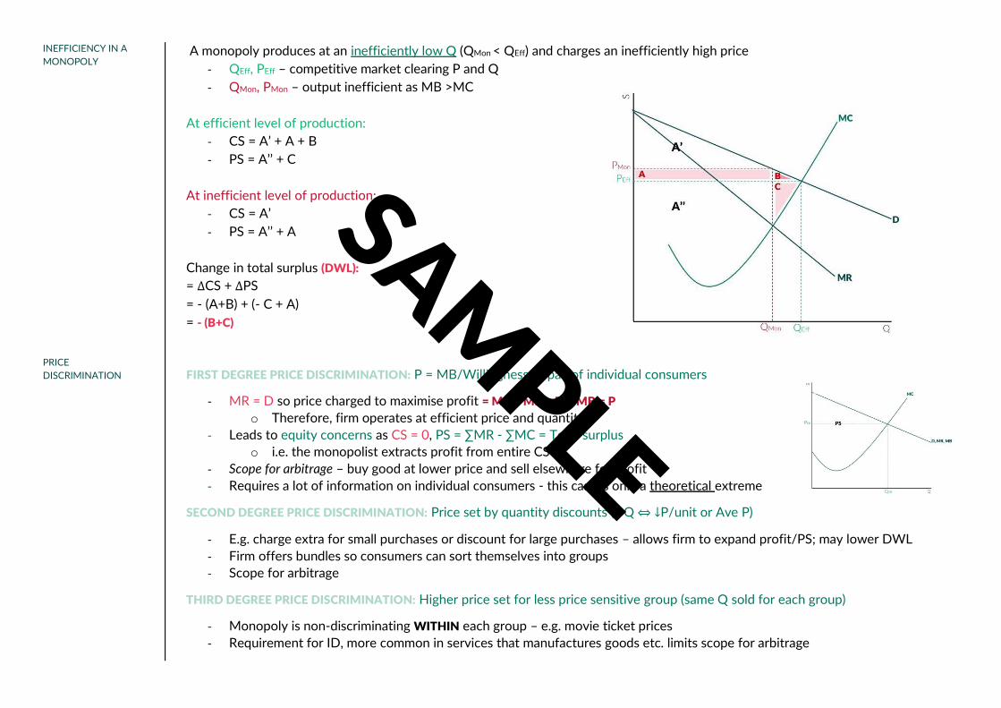
A monopoly produces at an inefficiently low Q (QMon < QEff) and charges an inefficiently high price

- QEff, PEff – competitive market clearing P and Q

- QMon, PMon – output inefficient as MB >MC

At efficient level of production:

- CS = A’ + A + B

- PS = A’’ + C

At inefficient level of production:

- CS = A’

- PS = A’’ + A

Change in total surplus (DWL):

= ∆CS + ∆PS

= - (A+B) + (- C + A)

= - (B+C)

FIRST DEGREE PRICE DISCRIMINATION: P = MB/Willingness to pay of individual consumers

- MR = D so price charged to maximise profit = MC = MR = D = MB = P

o Therefore, firm operates at efficient price and quantity

- Leads to equity concerns as CS = 0, PS = ∑MR - ∑MC = Total surplus

o i.e. the monopolist extracts profit from entire CS

- Scope for arbitrage – buy good at lower price and sell elsewhere for profit

- Requires a lot of information on individual consumers - this case is only a theoretical extreme

SECOND DEGREE PRICE DISCRIMINATION: Price set by quantity discounts (↑ Q ⇔ ↓P/unit or Ave P)

- E.g. charge extra for small purchases or discount for large purchases – allows firm to expand profit/PS; may lower DWL

- Firm offers bundles so consumers can sort themselves into groups

- Scope for arbitrage

THIRD DEGREE PRICE DISCRIMINATION: Higher price set for less price sensitive group (same Q sold for each group)

- Monopoly is non-discriminating WITHIN each group – e.g. movie ticket prices

- Requirement for ID, more common in services that manufactures goods etc. limits scope for arbitrage

SAMPLE

MONOPOLISTIC

COMPETITION

PRODUCT

DIFFERENTIATION

CONDITIONS FOR AN

MC INDUSTRY

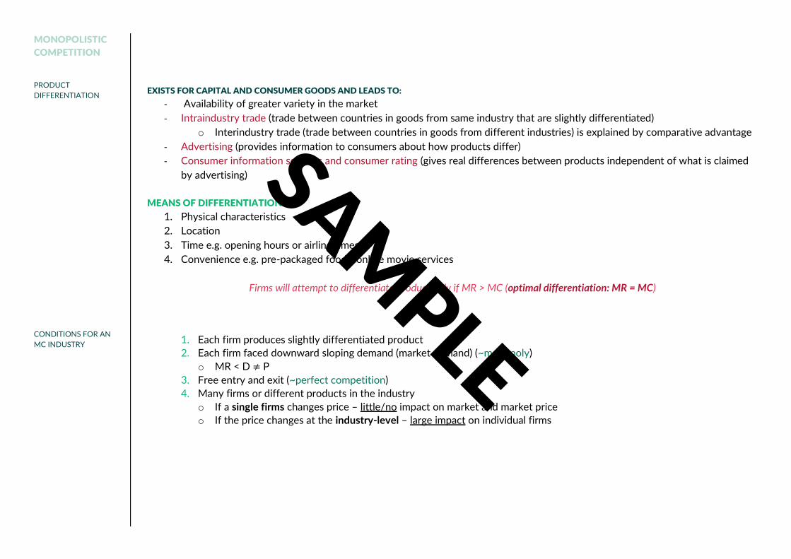
EXISTS FOR CAPITAL AND CONSUMER GOODS AND LEADS TO:

- Availability of greater variety in the market

- Intraindustry trade (trade between countries in goods from same industry that are slightly differentiated)

o Interindustry trade (trade between countries in goods from different industries) is explained by comparative advantage

- Advertising (provides information to consumers about how products differ)

- Consumer information services and consumer rating (gives real differences between products independent of what is claimed

by advertising)

MEANS OF DIFFERENTIATION:

1. Physical characteristics

2. Location

3. Time e.g. opening hours or airline times

4. Convenience e.g. pre-packaged foods, online movie services

Firms will attempt to differentiate product only if MR > MC (optimal differentiation: MR = MC)

1. Each firm produces slightly differentiated product

2. Each firm faced downward sloping demand (market demand) (~monopoly)

o MR < D ≠ P

3. Free entry and exit (~perfect competition)

4. Many firms or different products in the industry

o If a single firms changes price – little/no impact on market and market price

o If the price changes at the industry-level – large impact on individual firms

SAMPLE