Embed Size (px)
Citation preview
SamplingDistribution
Ching-Han Hsu,Ph.D.
Populations andSamples
Some ImportantStatistics
SamplingDistributionsSampling Distribution ofMean
Sampling Distribution ofSample Variance
8.1
Lecture #8Sampling Distribution
BMIR Lecture Series on Probability and Statistics
Ching-Han Hsu, Ph.D.Department of Biomedical Engineering
and Environmental SciencesNational Tsing Hua University
SamplingDistribution
Ching-Han Hsu,Ph.D.
Populations andSamples
Some ImportantStatistics
SamplingDistributionsSampling Distribution ofMean
Sampling Distribution ofSample Variance
8.2
Populations
Definition
A population consists of the totality of the observationswith which we are concerned.
• The totality of observations, whether their number befinite or infinite, constitutes what we call apopulation.
• The word population previously referred toobservations obtained from statistical studies aboutpeople.
• Today, statisticians use the term to refer toobservations relevant to anything of interest, whetherit be groups of people, animals, or all possibleoutcomes from some complicated biological orengineering system.
SamplingDistribution
Ching-Han Hsu,Ph.D.
Populations andSamples
Some ImportantStatistics
SamplingDistributionsSampling Distribution ofMean
Sampling Distribution ofSample Variance
8.3
Populations: Examples
• If there 600 students in the school whom weclassified according to blood type, we say that wehave a population of size 600.
• The number of the cards in a deck, the heights ofresidents in a city, and the lengths of cars in aparking lot are examples of populations with finitenumber. The total number of observations is also afinite number.
• The observations obtained by measuring theatmospheric pressure every day or all measurementsof the depth of a lake are examples of populationswhose sizes are infinite.
SamplingDistribution
Ching-Han Hsu,Ph.D.
Populations andSamples
Some ImportantStatistics
SamplingDistributionsSampling Distribution ofMean
Sampling Distribution ofSample Variance
8.4
An Observation
• Each observation in a population is a value of arandom variable X having some probabilitydistribution f (x).
• For example, if one is inspecting items coming off anassembly line for detect, then each observation inthe population might be a value 0 or 1 of the Bernoullirandom variable X with probability distribution
b(x : 1, p) = pxq1−x, x = 0, 1
where 0 indicates a non-defective item and 1indicates a defective one. p is the probability of anyitem being defective and q = 1− p.
• When we refer to the population f (x), i.e, binomial ornormal distributions, we mean a population whoseobservations are values of a random variable havingthe probability distribution f (x).

SamplingDistribution
Ching-Han Hsu,Ph.D.
Populations andSamples
Some ImportantStatistics
SamplingDistributionsSampling Distribution ofMean
Sampling Distribution ofSample Variance
8.5
Sampling
Definition
A sample is a subset of population.
• In the statistical inference, statisticians are interestedin arriving at conclusions concerning a populationwhen it is impossible or impractical to observe theentire set of observations that make up thepopulation.
• We must depend on a subset of observations fromthe population to help us make inferencesconcerning that same population.
• If our inferences are to be valid, we must obtainsamples that are representative of the population.
• Any sampling procedure that produces inferencesthat consistently over-estimate or consistentlyunder-estimate some characteristic of the populationis said to be biased.
SamplingDistribution
Ching-Han Hsu,Ph.D.
Populations andSamples
Some ImportantStatistics
SamplingDistributionsSampling Distribution ofMean
Sampling Distribution ofSample Variance
8.6
Random Sample
Definition
Let X1,X2, . . . ,Xn be n independent random variables,each having the same probability distribution functionf (x). Define X1,X2, . . . ,Xn to be a random sample of sizen from the population f (x) and write its joint probabilitydistribution as
f (x1, x2, . . . , xn) = f (x1)f (x2) · · · f (xn)
• In a random sample, the observations are madeindependently and at random.
• The random variable Xi, i = 1, . . . , n represents theith measurement or sample value that we observe.
• And xi, i = 1, . . . , n represents the real value that wemeasure.
SamplingDistribution
Ching-Han Hsu,Ph.D.
Populations andSamples
Some ImportantStatistics
SamplingDistributionsSampling Distribution ofMean
Sampling Distribution ofSample Variance
8.7
Statistics
Definition
Any function of the random variables constituting arandom sample is called a statistic.
Statistical Inferences• We want some methods to make decisions or to
draw conclusions about a population.• We need samples from population and utilize the
information within.• The methods can be divided into two major areas:
parameter estimation and hypothesis testing.What is statistics?• Statistics is a function of observations or random
samples.• Statistics itself is also a random variable.• The probability distribution of a statistics is called a
sampling distribution.
SamplingDistribution
Ching-Han Hsu,Ph.D.
Populations andSamples
Some ImportantStatistics
SamplingDistributionsSampling Distribution ofMean
Sampling Distribution ofSample Variance
8.8
Location Measures of a Sample
Let X1,X2, . . . ,Xn represent n random variables.• Sample Mean:
X =1n
n∑i=1
Xi
Note that the statistic X assume the valuex = 1
n
∑ni=1 xi.
• Sample Median:
x =
x(n+1)/2, if n is odd,12(xn/2 + xn/2+1), if n is even
where the observations, x1, x2, . . . , xn, are arranged inincreasing order.
• The sample mode is the value of the sample thatoccurs most often.
SamplingDistribution
Ching-Han Hsu,Ph.D.
Populations andSamples
Some ImportantStatistics
SamplingDistributionsSampling Distribution ofMean
Sampling Distribution ofSample Variance
8.9
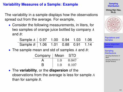
Variability Measures of a Sample: Example
The variability in a sample displays how the observationsspread out from the average. For example,• Consider the following measurements, in liters, for
two samples of orange juice bottled by company Aand B:
Sample A 0.97 1.00 0.94 1.03 1.06Sample B 1.06 1.01 0.88 0.91 1.14
• The sample mean and std of samples A and B:Company Mean STD
A 1.0 0.047B 1.0 0.107
• The variability, or the dispersion of theobservations from the average is less for sample Athan for sample B.
SamplingDistribution
Ching-Han Hsu,Ph.D.
Populations andSamples
Some ImportantStatistics
SamplingDistributionsSampling Distribution ofMean
Sampling Distribution ofSample Variance
8.10
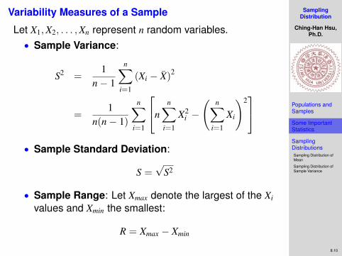
Variability Measures of a Sample
Let X1,X2, . . . ,Xn represent n random variables.• Sample Variance:
S2 =1
n− 1
n∑i=1
(Xi − X)2
=1
n(n− 1)
n∑i=1
nn∑
i=1
X2i −
(n∑
i=1
Xi
)2
• Sample Standard Deviation:
S =√
S2
• Sample Range: Let Xmax denote the largest of the Xi
values and Xmin the smallest:
R = Xmax − Xmin
SamplingDistribution
Ching-Han Hsu,Ph.D.
Populations andSamples
Some ImportantStatistics
SamplingDistributionsSampling Distribution ofMean
Sampling Distribution ofSample Variance
8.11
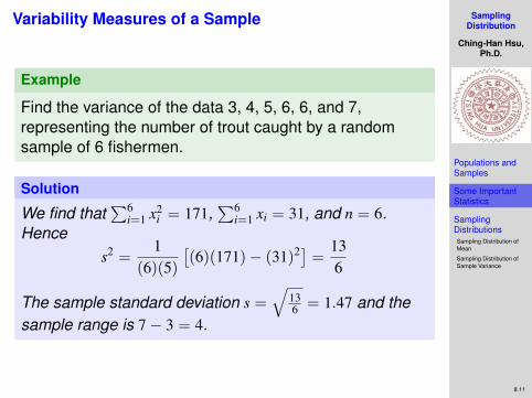
Variability Measures of a Sample
Example
Find the variance of the data 3, 4, 5, 6, 6, and 7,representing the number of trout caught by a randomsample of 6 fishermen.
Solution
We find that∑6
i=1 x2i = 171,
∑6i=1 xi = 31, and n = 6.
Hences2 =
1(6)(5)
[(6)(171)− (31)2] =
136
The sample standard deviation s =√
136 = 1.47 and the
sample range is 7− 3 = 4.
SamplingDistribution
Ching-Han Hsu,Ph.D.
Populations andSamples
Some ImportantStatistics
SamplingDistributionsSampling Distribution ofMean
Sampling Distribution ofSample Variance
8.12
Sampling Distribution
Definition
The probability distribution of a statistic is called asampling distribution.
• Since a statistic is a random variable that dependsonly on the observed samples, it must have aprobability distribution.
• The sampling distribution of a statistic depends onthe distribution of the population, the size of thesamples, and the method of choosing the samples.
SamplingDistribution
Ching-Han Hsu,Ph.D.
Populations andSamples
Some ImportantStatistics
SamplingDistributionsSampling Distribution ofMean
Sampling Distribution ofSample Variance
8.13
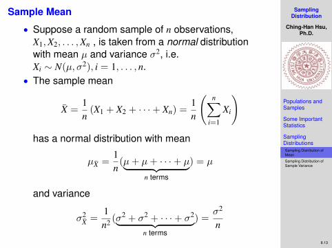
Sample Mean
• Suppose a random sample of n observations,X1,X2, . . . ,Xn , is taken from a normal distributionwith mean µ and variance σ2, i.e.Xi ∼ N(µ, σ2), i = 1, . . . , n.
• The sample mean
X =1n
(X1 + X2 + · · ·+ Xn) =1n
(n∑
i=1
Xi
)has a normal distribution with mean
µX =1n
(µ+ µ+ · · ·+ µ︸ ︷︷ ︸n terms
) = µ
and variance
σ2X =
1n2 (σ2 + σ2 + · · ·+ σ2︸ ︷︷ ︸
n terms
) =σ2
n
SamplingDistribution
Ching-Han Hsu,Ph.D.
Populations andSamples
Some ImportantStatistics
SamplingDistributionsSampling Distribution ofMean
Sampling Distribution ofSample Variance
8.14
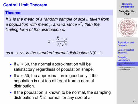
Central Limit Theorem
Theorem
If X is the mean of a random sample of size n taken froma population with mean µ and variance σ2, then thelimiting form of the distribution of
Z =X − µσ/√
n,
as n→∞, is the standard normal distribution N(0, 1).
• If n ≥ 30, the normal approximation will besatisfactory regardless of population shape.
• If n < 30, the approximation is good only if thepopulation is not too different from a normaldistribution.
• If the population is known to be normal, the samplingdistribution of X is normal for any size of n.
SamplingDistribution
Ching-Han Hsu,Ph.D.
Populations andSamples
Some ImportantStatistics
SamplingDistributionsSampling Distribution ofMean
Sampling Distribution ofSample Variance
8.15
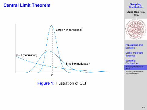
Central Limit Theorem
Figure 1: Illustration of CLT
SamplingDistribution
Ching-Han Hsu,Ph.D.
Populations andSamples
Some ImportantStatistics
SamplingDistributionsSampling Distribution ofMean
Sampling Distribution ofSample Variance
8.16
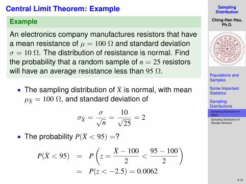
Central Limit Theorem: Example
Example
An electronics company manufactures resistors that havea mean resistance of µ = 100 Ω and standard deviationσ = 10 Ω. The distribution of resistance is normal. Findthe probability that a random sample of n = 25 resistorswill have an average resistance less than 95 Ω.
• The sampling distribution of X is normal, with meanµX = 100 Ω, and standard deviation of
σX =σ√n
=10√25
= 2
• The probability P(X < 95) =?
P(X < 95) = P(
z =X − 100
2<
95− 1002
)= P(z < −2.5) = 0.0062
SamplingDistribution
Ching-Han Hsu,Ph.D.
Populations andSamples
Some ImportantStatistics
SamplingDistributionsSampling Distribution ofMean
Sampling Distribution ofSample Variance
8.17
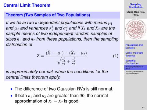
Central Limit Theorem
Theorem (Two Samples of Two Populations)
If we have two independent populations with means µ1and µ2 and variances σ2
1 and σ22 and if X1 and X2 are the
sample means of two independent random samples ofsizes n1 and n2 from these populations, then the samplingdistribution of
Z =(X1 − µ1)− (X2 − µ2)√
σ21
n1+
σ22
n2
(1)
is approximately normal, when the conditions for thecentral limits theorem apply.
• The difference of two Gaussian RVs is still normal.• If both n1 and n2 are greater than 30, the normal
approximation of X1 − X2 is good.
SamplingDistribution
Ching-Han Hsu,Ph.D.
Populations andSamples
Some ImportantStatistics
SamplingDistributionsSampling Distribution ofMean
Sampling Distribution ofSample Variance
8.18
Central Limit Theorem: Example
Example
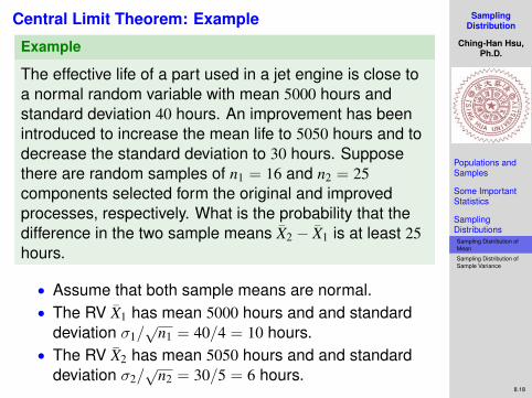
The effective life of a part used in a jet engine is close toa normal random variable with mean 5000 hours andstandard deviation 40 hours. An improvement has beenintroduced to increase the mean life to 5050 hours and todecrease the standard deviation to 30 hours. Supposethere are random samples of n1 = 16 and n2 = 25components selected form the original and improvedprocesses, respectively. What is the probability that thedifference in the two sample means X2 − X1 is at least 25hours.
• Assume that both sample means are normal.• The RV X1 has mean 5000 hours and and standard
deviation σ1/√
n1 = 40/4 = 10 hours.• The RV X2 has mean 5050 hours and and standard
deviation σ2/√
n2 = 30/5 = 6 hours.
SamplingDistribution
Ching-Han Hsu,Ph.D.
Populations andSamples
Some ImportantStatistics
SamplingDistributionsSampling Distribution ofMean
Sampling Distribution ofSample Variance
8.19
Central Limit Theorem: Example
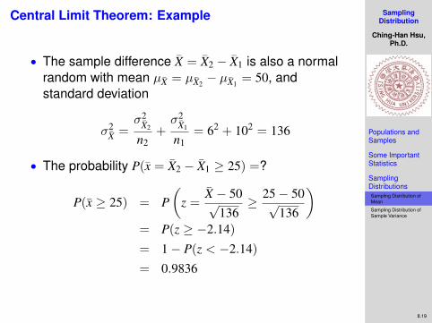
• The sample difference X = X2 − X1 is also a normalrandom with mean µX = µX2
− µX1= 50, and
standard deviation
σ2X =
σ2X2
n2+σ2
X1
n1= 62 + 102 = 136
• The probability P(x = X2 − X1 ≥ 25) =?
P(x ≥ 25) = P(
z =X − 50√
136≥ 25− 50√
136
)= P(z ≥ −2.14)
= 1− P(z < −2.14)
= 0.9836
SamplingDistribution
Ching-Han Hsu,Ph.D.
Populations andSamples
Some ImportantStatistics
SamplingDistributionsSampling Distribution ofMean
Sampling Distribution ofSample Variance
8.20
Two Samples: Example
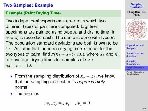
Example (Paint Drying Time)
Two independent experiments are run in which twodifferent types of paint are computed. Eighteenspecimens are painted using type A, and drying time (inhours) is recorded each. The same is done with type B.The population standard deviations are both known to be1.0. Assume that the mean drying time is equal for thetwo types of paint, find P(XA − XB > 1.0), where XA and Xb
are average drying times for samples of sizenA = nB = 18.
• From the sampling distribution of XA − XB, we knowthat the sampling distribution is approximatelynormal.
• The mean is
µXA−XB= µXA
− µXB= 0
SamplingDistribution
Ching-Han Hsu,Ph.D.
Populations andSamples
Some ImportantStatistics
SamplingDistributionsSampling Distribution ofMean
Sampling Distribution ofSample Variance
8.21
Two Samples: Example
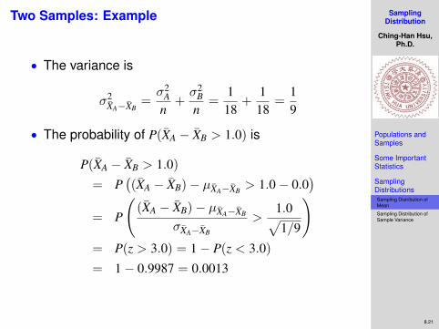
• The variance is
σ2XA−XB
=σ2
An
+σ2
B
n=
118
+1
18=
19
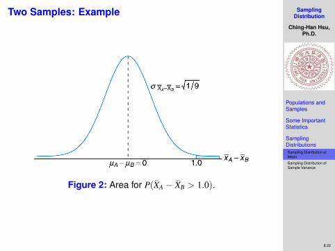
• The probability of P(XA − XB > 1.0) is
P(XA − XB > 1.0)
= P((XA − XB)− µXA−XB
> 1.0− 0.0)
= P
((XA − XB)− µXA−XB
σXA−XB
>1.0√1/9
)= P(z > 3.0) = 1− P(z < 3.0)
= 1− 0.9987 = 0.0013
SamplingDistribution
Ching-Han Hsu,Ph.D.
Populations andSamples
Some ImportantStatistics
SamplingDistributionsSampling Distribution ofMean
Sampling Distribution ofSample Variance
8.22
Two Samples: Example
Figure 2: Area for P(XA − XB > 1.0).
SamplingDistribution
Ching-Han Hsu,Ph.D.
Populations andSamples
Some ImportantStatistics
SamplingDistributionsSampling Distribution ofMean
Sampling Distribution ofSample Variance
8.23
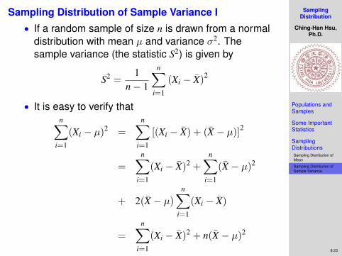
Sampling Distribution of Sample Variance I• If a random sample of size n is drawn from a normal
distribution with mean µ and variance σ2. Thesample variance (the statistic S2) is given by
S2 =1
n− 1
n∑i=1
(Xi − X)2
• It is easy to verify thatn∑
i=1
(Xi − µ)2 =
n∑i=1
[(Xi − X) + (X − µ)]2
=
n∑i=1
(Xi − X)2 +
n∑i=1
(X − µ)2
+ 2(X − µ)
n∑i=1
(Xi − X)
=
n∑i=1
(Xi − X)2 + n(X − µ)2
SamplingDistribution
Ching-Han Hsu,Ph.D.
Populations andSamples
Some ImportantStatistics
SamplingDistributionsSampling Distribution ofMean
Sampling Distribution ofSample Variance
8.24
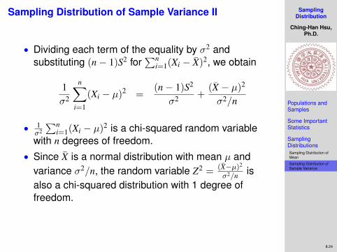
Sampling Distribution of Sample Variance II
• Dividing each term of the equality by σ2 andsubstituting (n− 1)S2 for
∑ni=1(Xi − X)2, we obtain
1σ2
n∑i=1
(Xi − µ)2 =(n− 1)S2
σ2 +(X − µ)2
σ2/n
• 1σ2
∑ni=1(Xi − µ)2 is a chi-squared random variable
with n degrees of freedom.• Since X is a normal distribution with mean µ and
variance σ2/n, the random variable Z2 = (X−µ)2
σ2/n isalso a chi-squared distribution with 1 degree offreedom.
SamplingDistribution
Ching-Han Hsu,Ph.D.
Populations andSamples
Some ImportantStatistics
SamplingDistributionsSampling Distribution ofMean
Sampling Distribution ofSample Variance
8.25
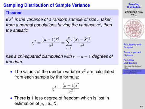
Sampling Distribution of Sample Variance
Theorem
If S2 is the variance of a random sample of size n takenfrom a normal populations having the variance σ2, thenthe statistic
χ2 =(n− 1)S2
σ2 =
n∑i=1
(Xi − X)2
σ2
has a chi-squared distribution with ν = n− 1 degrees offreedom.
• The values of the random variable χ2 are calculatedfrom each sample by the formula:
χ2 =(n− 1)s2
σ2
• There is 1 less degree of freedom which is lost inestimation of µ, i.e., X.
SamplingDistribution
Ching-Han Hsu,Ph.D.
Populations andSamples
Some ImportantStatistics
SamplingDistributionsSampling Distribution ofMean
Sampling Distribution ofSample Variance
8.26
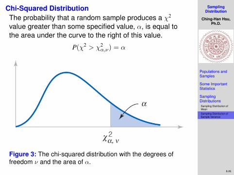
Chi-Squared DistributionThe probability that a random sample produces a χ2
value greater than some specified value, α, is equal tothe area under the curve to the right of this value.
P(χ2 > χ2α,ν) = α
Figure 3: The chi-squared distribution with the degrees offreedom ν and the area of α.
SamplingDistribution
Ching-Han Hsu,Ph.D.
Populations andSamples
Some ImportantStatistics
SamplingDistributionsSampling Distribution ofMean
Sampling Distribution ofSample Variance
8.27
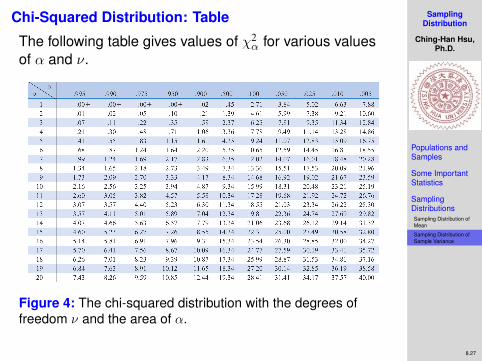
Chi-Squared Distribution: Table
The following table gives values of χ2α for various values
of α and ν.
Figure 4: The chi-squared distribution with the degrees offreedom ν and the area of α.
SamplingDistribution
Ching-Han Hsu,Ph.D.
Populations andSamples
Some ImportantStatistics
SamplingDistributionsSampling Distribution ofMean
Sampling Distribution ofSample Variance
8.28
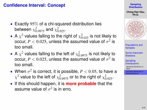
Confidence Interval: Concept
• Exactly 95% of a chi-squared distribution liesbetween χ2
0.0975 and χ20.025.
• A χ2 values falling to the right of χ20.025 is not likely to
occur, P < 0.025, unless the assumed value of σ2 istoo small.
• A χ2 values falling to the left of χ20.0975 is not likely to
occur, P < 0.025, unless the assumed value of σ2 istoo small.
• When σ2 is correct, it is possible, P < 0.05, to have aχ2 value to the left of χ2
0.0975 or to the right of χ20.025.
• If this should happen, it is more probable that theassume value of σ2 is in erro.
SamplingDistribution
Ching-Han Hsu,Ph.D.
Populations andSamples
Some ImportantStatistics
SamplingDistributionsSampling Distribution ofMean
Sampling Distribution ofSample Variance
8.29
Sampling Distribution of Sample Variance: Example
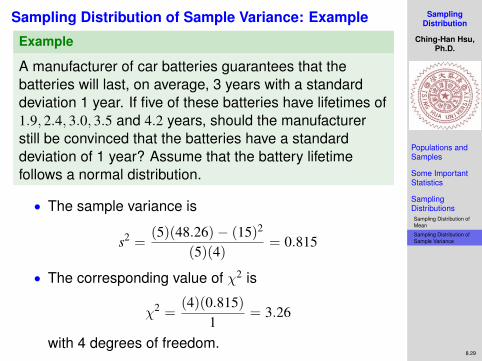
Example
A manufacturer of car batteries guarantees that thebatteries will last, on average, 3 years with a standarddeviation 1 year. If five of these batteries have lifetimes of1.9, 2.4, 3.0, 3.5 and 4.2 years, should the manufacturerstill be convinced that the batteries have a standarddeviation of 1 year? Assume that the battery lifetimefollows a normal distribution.
• The sample variance is
s2 =(5)(48.26)− (15)2
(5)(4)= 0.815
• The corresponding value of χ2 is
χ2 =(4)(0.815)
1= 3.26
with 4 degrees of freedom.
SamplingDistribution
Ching-Han Hsu,Ph.D.
Populations andSamples
Some ImportantStatistics
SamplingDistributionsSampling Distribution ofMean
Sampling Distribution ofSample Variance
8.30
Sampling Distribution of Sample Variance: Example
• Since the 95% of the χ2 values with 4 degrees offreedom fall between 0.484 and 11.143.
• Since 0.484 < 3.26 < 11.143, the computed value isreasonable.
• The manufacturer has no reason to suspect thestandard deviation is other than 1 year.
SamplingDistribution
Ching-Han Hsu,Ph.D.
Populations andSamples
Some ImportantStatistics
SamplingDistributionsSampling Distribution ofMean
Sampling Distribution ofSample Variance
8.31
Chi-Squared Distribution
Theorem
If the random variable X is N(µ, σ2), then the randomvariable Y = (X−µ)2
σ2 = Z2 is χ2(1).
• Z = (X−µ)σ is N(0, 1).
• Since fY(y) = 12√
y [fX(√
y) + fX(−√y)],
fY(y) =1
21/2√πy1/2−1e−y/2
=1
Γ(12)
(12
)1/2
y1/2−1e−y/2
= fY(y; γ = 1/2, λ = 1/2) =λγxγ−1e−λx
Γ(γ)
= χ2(1) = χ2(ν = 1)
SamplingDistribution
Ching-Han Hsu,Ph.D.
Populations andSamples
Some ImportantStatistics
SamplingDistributionsSampling Distribution ofMean
Sampling Distribution ofSample Variance
8.32
MGFs of Gamma Distributions
• If X is a Gamma distribution with pdf
f (x; γ, λ) =
λγ
Γ(γ)xγ−1e−λx, 0 < x <∞0, elsewhere
,
then the MGF of the random variable X is
MX(t) =1
(1− t/λ)γ
• The MGF of the chi-squared distribution with 1degree of freedom , χ2(1),is, i.e., λ = 1/2, γ = ν/2and ν = 1
MX(t) =1
(1− 2t)1/2
SamplingDistribution
Ching-Han Hsu,Ph.D.
Populations andSamples
Some ImportantStatistics
SamplingDistributionsSampling Distribution ofMean
Sampling Distribution ofSample Variance
8.33
MGFs of Gamma Distributions
• If X1,X2, . . . ,Xn are independent random variableswith moment generating functionsMX1(t),MX2(t), . . . ,MXn(t), respectively, and ifY = X1 + X2 + · · ·+ Xn then the moment generatingfunction of Y is
MY(t) = MX1(t) ·MX2(t) · · · · ·MXn(t)
• If each Xi, i = 1, . . . , n has a χ2(1) distribution, thenthe MGF of Y is
MY(t) =
n∏i=1
1(1− 2t)1/2 =
1(1− 2t)n/2
which is also a chi-squared distribution with ndegrees of freedom, χ2(n).